Modulation codes

Modulation codes

Proefschrift

ter verkrijging van de graad van doctor aan deTechnische Universiteit Eindhoven, op gezag vande Rector Magnificus, prof.dr. M. Rem, vooreen commissie aangewezen door het College vanDekanen in het openbaar te verdedigen op

dinsdag 17 december 1996 om 16.00 uur

door

Hendrik Dirk Lodewijk Hollmanngeboren te Utrecht

Dit proefschrift is goedgekeurd door de promotoren:prof.dr. J.H. van Lintenprof.dr. P.H. Siegel

CIP-gegevens Koninklijke Bibliotheek, Den HaagHollmann. H.D.L.Modulation codesProefschrift Technische Universiteit Eindhoven.-Met lit. opg.,-Met samenvatting in het Nederlands.ISBN 90-74445-32-2Trefw.: modulatie code, digitaal, communicatie

The work described in this thesis has been carried outat the PHILIPS RESEARCH LABORATORIES Eindhoven,the Netherlands, as part of the Philips Research Programme.

@Philips Electronics N.V. 1996All rights are reserved. Reproduction in whole or in part is

prohibited without the written consent of the copyright owner.

Acknowledgments

This work has been carried out at the Philips Research Laboratories in Eindhoven.I am indebted to the management, and in particular to my group leader Cees Stam,for providing the opportunity to write this thesis. Furthermore, I warmly thank mycolleagues Ludo Tolhuizen and Stan Baggen, who in various stages read most ofthis work and who proposed innumerable improvements.

It is a pleasure for me to express my gratitude to Kees Schouhamer Immink,co-author of Chapters II and III, who introduced me to the field of modulationcodes and to many of the people involved. This work has greatly benefited fromhis guidance and insight, and from the many stimulating discussions that weshared.

I also wish to thank my promotor and former teacher Jack van Lint for valu­able suggestions concerning the presentation of my work. His everlasting enthu­siasm for and interest in mathematics has always been a great example to me. Iwas proud to be his pupil, and it is an honour to have him as my promotor now.

The thoughtful criticisms and suggestions of Brian Marcus have added greatlyto the second part of this work. His careful reading of the manuscript saved mefrom some later embarrassment. I am very grateful for his stimulations and hisinterest in my work.

I would also like to thank my promotor Paul Siegel and the other members onmy committee for their time and efforts.

This thesis is typeset with ~TEX, in the teTEX distribution from Thomas Esserand using Times-Roman fonts in combination with the mathtime font package ofMichael Spivak. Special thanks are due to Jan van der Steen and Olaf Weber,both from CWI, Amsterdam, and to my colleague Ronald van Rijn, for theirindispensable help with the installation of teTEX and for many other efforts.

Finally, a most warm thanks goes to my wife Brigitte and our kids Kirsten,Sanne, Line, and Tommie, for their encouragement and support-offered on thescarce occasions when we did meet :-)

Contellts

1 Introduction1.1 Digital communication

1.1.1 AID conversion . .1.1.2 Data-compression1.1.3 Protection against errors; error-correcting codes .

1.2 Modulation codes . . . . . . . . . . . . . . . . .J.2.1 Type of constraints; constrained systems.1.2.2 Coding rate and capacity . . . . . . . . .1.2.3 The capacity of constraints of finite type.1.2.4 Sofic systems and their capacity1.2.5 Encoding and encoders .1.2.6 Decoding and decoders . . .1.2.7 Synchronization .1.2.8 Code-construction methods

1.3 Overview of the contents of this thesisReferences. . . . . . . . . . . . . . .

2 Performance of Efficient Balanced Codes2.1 Introduction..............2.2 Balancing of Codewords . . . . . . .2.3 Spectrum and sum variance of sequences.2.4 A counting problem . .2.5 Performance Appraisal2.6 Conclusions....

AcknowledgementReferences. . . . .

12346

II1114

1620252729304547

535355565865656666

3 Prefix-synchronized Runlength-Iimited Sequences3.1 Introduction .

69. . . . . . . . .. 70

xii

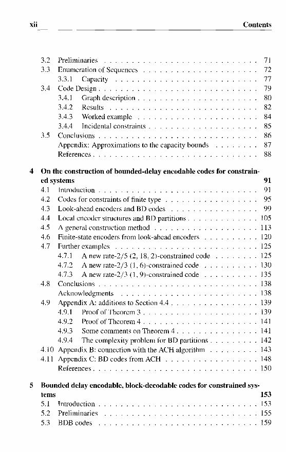
3.2 Preliminaries . . . . . . .3.3 Enumeration of Sequences

3.3.1 Capacity .3.4 Code Design .

3.4.1 Graph description.3.4.2 Results . . . . . .3.4.3 Worked example .3.4.4 Incidental constraints .

3.5 Conclusions .Appendix: Approximations to the capacity boundsReferences. . . . . . . . . . . . . . . . . . . . . .

Contents

7172777980828485868788

4 On the construction of bounded-delay encodable codes for constrain-ed systems 914.1 Introduction............. 914.2 Codes for constraints of finite type . 954.3 Look-ahead encoders and BD codes 994.4 Local encoder structures and BD partitions. 1054.5 A general construction method . . . . . . . 1134.6 Finite-state encoders from look-ahead encoders 1204.7 Further examples . . . . . . . . . . . . . . . . 125

4.7.1 A new rate-2/5 (2,18, 2)-constrained code 1254.7.2 A new rate-2/3 (1, 6)-constrained code 1304.7.3 A new rate-2/3 (1, 9)-constrained code 135

4.8 Conclusions.............. 138Acknowledgments 138

4.9 Appendix A: additions to Section 4.4 . 1394.9.1 Proof of Theorem 3 . . . . . . 1394.9.2 Proof of Theorem 4 . . . . . . 1414.9.3 Some comments on Theorem 4. 1414.9.4 The complexity problem for BD partitions. 142

4.10 Appendix B: connection with the ACH algorithm 1434.11 Appendix C: BD codes from ACH 148

References. . . . . . . . . . . . . . . . . . . . . 150

5 Bounded delay encodable, block-decodable codes for constrained sys-tems 1535.1 Introduction. 1535.2 Preliminaries 1555.3 BDB codes . 159

Contents xiii

5.4 Principal state-sets for one-symbol look-ahead BDB codes 1635.5 State-trees for M-symbollook-ahead BDB codes 1665.6 The state combination method 1735.7 Stable state-sets . . 1775.8 Discussion..... 181

Acknowledgments 181Appendix A 181Appendix B 183References . 185

6 A block-decodable (d, k) = (1,8) runlength-limited rate 8/12 code 1876.1 Introduction............. 1876.2 Principal state-sets for BDB codes . 1896.3 Begin and end types of code words. 1916.4 Description of the code 1936.5 Discussion..... 195

Acknowledgement ]96References. . . . . 197

7 On an approximate eigenvector associated with a modulation code 1997.1 Introduction....... 1997.2 Notation and background . . . . . . . . . . 2017.3 Preliminaries . . . . . . . . 2047.4 The number of children in N of paths in M 2057.5 How M and C determine ij 2077.6 Main results. 2087.7 Some remarks 2097.8 Applications. 2107.9 Discussion.. 213

Appendix: Some examples 214References. . . . . . . . . 215

Summary 217

Samenvatting 223

Curriculum Vitae 229

Index 231

Chapter 1

Introduction

Modulation codes, the topic of this thesis, are one of the elements employed in adigital communication system. We are all familiar with these highly efficient andreliable means to transport information in time or in place, in the shape of, e.g.,a CD-player, a computer, or possibly a modem or a fax. In this chapter, we areinterested in the principles that makes them work.

In Section 1.1 we position modulation and modulation codes within a digitalcommunication scheme. We first present the usual sender-channel-receiver modelfor such systems and indicate the function of the other elements composing it:analogue-to-digital conversion, data compression and error-protection.Here, wewill see that modulation codes function nearest to the channel and are designedto ensure that the data-stream attains certain properties that are beneficial duringsubsequent transmission or storage.

In separate subsections, we present a mathematician's view on the other ele­ments of the system while keeping a firm eye on the practical significance of thediscussion. In Section 1.2 we provide the necessary background on modulationcodes, as detailed as needed to understand and appreciate the other parts of thisthesis. This chapter ends with Section 1.3, where we present an overview of thethesis.

We have tried to keep the presentation in this introductory chapter as simpleas possible. The only strict prerequisites are a working knowledge of elementarycalculus. At a few places, some familiarity with vectors and matrices is alsorequired. The material in Subsection 1.2.4, by far the most difficult part of thisintroduction, is important but need only be skimmed to understand most of whatcomes after it.

The subsequent six chapters consist of work that has previously appeared (orwill appear, in the case of Chapter 7) in international journals. We have used

2 1. Introduction

Ph

S

ysical Digital Compressed Protected Physical--- AID CaMP ECC MODignal Data Data Data Data

Noise

Channel

\De-Physical compressed Corrected Digital Physical~ DIA DECaMP DECC DEMODSignal Data Data Data Data

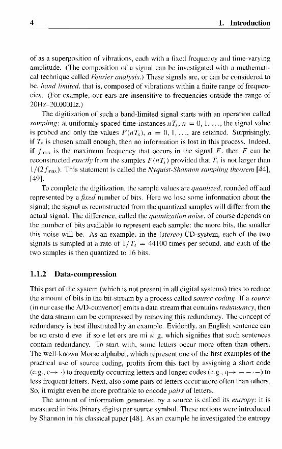
Figure 1: Schematical form ofa digital communication system.

the occasion to correct some minor mistakes in these papers, and we have alsoadded Appendix C to Chapter 4 and Appendix B to Chapter 5 in order to clmifycertain issues. We thank the IEEE-organization for its permission to reproduce thismaterial here. For a detailed overview of these chapters we refer to Section 1.3.

At the end of the thesis we provide an index for Chapter 1; this may be useful,e.g., to obtain information about concepts that the reader is assumed to be familiarwith in other chapters.

1.1 Digital communication

Present-day digital transmission or storage systems can be represented schemati­cally as in Figure 1. Such a digital communication system is usually considered asconsisting of three parts, the sender, the receiver, and the channel, the communi­cation pathway along which data can be transported, in some physical fatm, fromthe sender to the receiver. Here, the sender may be separated from the receivereither in place (transmission) or in time (storage). Due to the physical nature ofthe channel, the transmitted signal that carries the information will be corruptedby physical "noise" when it reaches the receiver. (Think of the effects of light­ning during transmission, or damaged areas of a disk.) The task of the system isto enable reliable communication even when this takes place over such a noisychannel.

At the sender's side, the analogue, physical input data (for example, the elec­trical current obtained when sound is captured by a microphone) is first passedthrough an AID converter where it is translated into digital form. Here withineach time-slot, an interval of time of some fixed duration, the continuously vary­ing physical data is approximated with the aid of a finite number of bits, quantumsof information each capable of holding either a "zero" or a "one". Then this dig-

1.1. Digital communication 3

ital source data, the stream of bits emitted by the AID converter, is compressed,an operation where we try to represent the same (or almost the same) informationwith fewer bits. The resulting bit-stream is then protected against errors by meansof an error-correcting code or ECC. Here, some redundancy is introduced, thatis, (redundant) bits are added to the bit-stream; as a result the original data canstill be recovered even if some errors occur, i.e., if some bit-values are changed.Finally, the bit-stream is modulated, prepared for "transmission over the channel"in some physical form. In the case of transmission, the transmitted signal mayconsist, e.g., of a sequence of constant-amplitude pulses of either A or - A unitsin amplitude and T seconds in duration, modulated by some carrier wave; in thecase of storage, the sequence of bits may be represented, e.g., by a sequence of pitsand lands (CD-system for optical recording) or by successive regions of positiveor negative magnetization (magnetic recording).

For various technical and physical reasons, some signals have a much lowerprobability than others to pass relatively unharmed through the channel. There­fore, it can be beneficial to avoid transmission of bit-streams that result in suchsignals. This can be achieved by employing a modulation code to transform thebit-stream into a channel-bit-stream that is more suitable for transmission over thechannel. As was the case for error-correcting codes, this adaptation to the channelnecessarily leads to an increase of the number of bits in the bit-stream.

At the receiver's side, the whole chain of events is reversed. First, the trans­mitted channel bits are recovered as well as possible from their physical form, aprocess called demodulation. At this stage, some of the channel bits will havean incorrect value, that is, they may contain errors. Some systems also asso­ciate reliability information with each recovered bit. Such information can bebeneficially employed in the subsequent data processing. Next, the resultingchannel-bit-stream is transformed back through the modulation code. Then theerror-correcting code is used to correct errors as much as possible, the data is de­compressed, and restored to something (hopefully) resembling its original physi­cal form by the D/A-converter.

We will now take some time to discuss these various parts of the system insome detail. All of them are (at least in part) based on some mathematical ideas;in our presentation we will concentrate on the mathematics that make them work.

1.1.1 AID conversion

We will model the physical data at the sender's input as areal-valued function F(t)

of the time t. For example, music can be described in physical terms as variationsin air-pressure. When captured by a microphone, these variations are translatedinto variations in electrical current. This function F, the signal, can be thought

4 1. Introduction

of as a superposition of vibrations, each with a fixed frequency and time-varyingamplitude. (The composition of a signal can be investigated with a mathemati­cal technique called Fourier analysis.) These signals are, or can be considered tobe, band-limited, that is, composed of vibrations within a finite range of frequen­cies. (For example, our ears are insensitive to frequencies outside the range of20Hz-20.000Hz.)

The digitization of such a band-limited signal starts with an operation calledsampling: at uniformly spaced time-instances nTs , n = 0, 1.... , the signal valueis probed and only the values F(nT~), n = 0,1, ... , are retained. Surprisingly,if Ts is chosen small enough, then no information is lost in this process. Indeed,if f max is the maximum frequency that occurs in the signal F, then F can bereconstructed exactly from the samples F (n T\) provided that T~ is not larger than1/(2fmax). This statement is called the Nyquist-Shannon sampling theorem [44],[49].

To complete the digitization, the sample values are quantized, rounded off andrepresented by afixed number of bits. Here we lose some information about thesignal; the signal as reconstructed from the quantized samples will differ from theactual signal. The difference, called the quantization noise, of course depends onthe number of bits available to represent each sample: the more bits, the smallerthis noise will be. As an example, in the (stereo) CD-system, each of the twosignals is sampled at a rate of 1/ T~ = 44100 times per second, and each of thetwo samples is then quantized to 16 bits.

1.1.2 Data-compression

This patt of the system (which is not present in all digital systems) tries to reducethe amount of bits in the bit-stream by a process called source coding. If a source(in our case the AID-convertor) emits a data stream that contains redundancy, thenthe data stream can be compressed by removing this redundancy. The concept ofredundancy is best illustrated by an example. Evidently, an English sentence canbe un ersto d eve if so e let ers are mi si g, which signifies that such sentencescontain redundancy. To start with, some letters occur more often than others.The well-known Morse alphabet, which represent one of the first examples of thepractical use of source coding, profits from this fact by assigning a short code(e.g., e---+ .) to frequently occurring letters and longer codes (e.g., q---+ - - .-) toless frequent letters. Next, also some pairs of letters occur more often than others.So, it might even be more profitable to encode pairs of letters.

The amount of information generated by a source is called its entropy; it ismeasured in bits (binary digits) per source symbol. These notions were introducedby Shannon in his classical paper [48]. As an example he investigated the entropy

1.1. Digital communication 5

of (a source emitting sentences in) the English language and found an estimateof about 1.3 bits per symbol, where the symbols are the 26 letters in the alphabettogether with the "space". That is, an English text can be represented with anaverage of about 1.3 bits per symbol; in other words, the average symbol in anEnglish sentence contains about 1.3 bits of information.

A particular way of representing sequences of source symbols emitted by asource (such as the Morse alphabet mentioned above) is called a source code. Theentropy of a source tells us the maximum possible compression rate, the maximumnumber of source symbols that can be represented by an average encoded bit of asource code for that source.

As a simple example, consider a source that emits four possible symbols "a","b", "c", and "d", where at each instant the probability that a particular one ofthese symbols is emitted next is 1/2,1/4, 1/8, and 1/8, respectively. We couldof course represent the four symbols by two bits each, as "00", "01", "10", and"11 ", respectively. Since each emitted symbol is either an "a" or not, with bothevents equally probable, it seems reasonable to suppose that the symbol "a" rep­resents one bit of information. Similarly, each event out of four possibilities canbe represented with two bits. If each of these events occurs with equal probability,it seems that each of them represents two bits of information. So we should thinkof the symbol "b" as representing two bits of information. A similar reasoningleads to the conclusion that each of the letters "c" and "d" represent three bits ofinformation. By a simple calculation we now find that the entropy, the averageamount of information per symbol, equals 1.75 bits per symbol. According tothis calculation, it should be possible to represent a stream of letters emitted bythis source by an average of only 1.75 bits per symbol, instead of with two bits asproposed earlier. This is indeed possible: encode the letters as

a -----+ 0, b -----+ 10, c -----+ 110, d -----+ 111.

Now each symbol is represented with the "correct" number of bits. Moreover, it isnot difficult to see that a stream of bits resulting from the encoding of a sequenceof letters can always be broken up into a sequence of encodings of symbols in oneand only one way (essentially, this is because the four "codewords" 0, 10, 110,and 11 1have the property that no one is the beginning of another one, that is, theyform a prefix code). Therefore, the original sequence can be exactly recoveredfrom the encoded sequence. As a consequence, distinct sequences have distinctencodings, which is of course a requirement for any alternative representation ofsource sequences.

So far, we have considered lossless source coding, that is, we required that theoriginal source output can be recovered exactly from its encoding. For some ap­plications, this requirement is too strict. For example, consider the case where the

6 1. Introduction

source emits video data (digitized pictures). Here, a slight degradation in picture­quality may well be acceptable. In such a case, it is sufficient that a sufficientlyclose approximation of the original can be recovered. If the encoding has thisproperty, then we speak of lossy source coding. The mathematical frameworkfor this case is called rate-distortion theory. This theory tells us, under certainassumptions about the source and the distortion measure, what is the highest pos­sible rate at which such a source may be encoded, given any maximum on theacceptable distortion. Unfortunately, practical sources tend not to satisfy these as­sumptions, but nevertheless a result as this can still give strong indications aboutwhat rates should be possible for such sources.

1.1.3 Protection against errors; error-correcting codes

When information in the form of a sequence of bits of a given length is sent over anoisy channel, then upon reception certain of the bits will have attained the wrongvalue; the sequence will contain errors. This raises the problem of how to enablereliable transmission over such a channel.

The problem can be understood as follows. If two transmitted sequences arealmost equal, then the channel can easily transform one into the other; in otherwords, the receiver cannot very well distinguish between corrupted versions ofsuch sequences. Therefore, we need to ensure that different transmitted sequencesare very different, or, as we say, we need to to create a sufficient amount of dis­tance between transmitted sequences. A common method to do so is by the inser­tion into the bit-stream of parity-cheek-bits, bits that hold the parity of the numberof "ones" among bits in certain given positions. An error-correcting code consistsof a collection of rules how to generate these parity-check-bits and where to insertthem, the encoding rules, together with the procedure to be used at the receiver'sside to handle the received sequence, i.e., how to detect and/or correct the errors,the decoding rules.

The fraction R of original bits or information bits in the resulting sequence iscalled the rate of the code; the quantity 1 - R is termed its redundancy. So thefewer bits are added, the higher the rate. The redundancy of a code reflects theprice that has to be paid for its error-protecting capabilities.

We can think of the decoding of a given received sequence as looking amongall possibly transmitted sequences for the one that has the highest probability ofhaving been sent (maximum-likelihood decoding). These probabilities of coursedepend on how the channel acts on the transmitted sequences.

In digital communication, an often-used channel-model is that of a binarysymmetric memoryless channel (BSMC): here we assume that each separate bithas a fixed probability p < 1/2 of being in error. In this model, the probability

1.1. Digital communication 7

that a certain sequence was sent, given the received sequence, only depends on theHamming distance of this sequence to the received sequence, where the distance ismeasured by the number of bit-positions in which these sequences differ. (Havinga few errors is more probable than having a great many of them.)

The number C = C(p) = - P log2 p- (1- p) log2(l- p) is called the capac­ity of the channel. (Unless specified otherwise, all logarithms will be to the base2.) One of the highlights of information theory, the mathematical theory of digi­tal communication, is a theorem obtained by Shannon in his landmark paper [48]which states that reliable communication over a BSMC is possible at any codingrate R < C. (A more precise statement is that for any given rate R < C and anyarbitrarily small number E > 0, there exist codes of rate R with the property thatthe word-error-probability after decoding is at most equal to E.) Remark that theway to achieve this is not simply to repeat each information bit a number of times!

The above theoretical result only holds "on the long run", that is when thenumber of transmitted bits gets larger and larger. (Obviously not much can beachieved if we only wish to transmit, e.g., a single bit.) Fortunately the resultstill approximately holds when the number of bits is very large but fixed. A moreserious problem is that no one knows how to construct such codes! (Facts suchas this, together with the almost religious admiration for Shannon amongst manytheoreticians, may explain why some of the more practice-oriented people do nothave a high regard of information theory as a practical science.) Indeed, althoughin fact Shannon showed that "almost every" code at the right rate has the desiredproperty, surprisingly all known constructed codes are much worse than what ac­cording to theory should be achievable. (Recently, some progress in this directionhas occurred with the invention of a class of codes called turbo codes [6]; for anrecent overview, see [5].) Although no codes fulfilling the promises of Shannon'stheorem are known, many families of codes have been constructed that enablereliable communication at a reasonable rate. Among the codes that have foundpractical use, we may distinguish two types: convolutional codes and block-codes.

Block-codes operate on sequences of a fixed length k, and transform eachsuch sequence into a codeword of a fixed length n by adding n - k parity-check­bits. (So the rate of the code equals kin.) When such codes are used to transmitlong sequences, the sequence is first grouped into words of length k and is thentransformed by the code into a sequence of n-bit codewords.

An important parameter of a block-code is its minimum distance, the mini­mum Hamming distance between any two different code sequences. A code withminimum distance d is capable of correcting e = L(d -l)/2J errors per codeword.That is, assuming that a received word contains at most e errors, it is possible torecover the original codeword. To see this, we first note that any received wordthat contains fewer than d12 errors has Hamming distance less than d12 to the

8 1. Introduction

originally transnritted codeword, but all other codewords, being at Hamming dis­tance at least d to this codeword, have Hamnring distance at least d /2 to thisword. (Think of such received words as being contained in a "sphere" with radiuse < d /2 centered around the originally transmitted codeword. As the centers ofall such spheres are at Hamming distance at least d, these spheres are all disjointand any word can be contained in at most one of them.) Hence the decoding rule"decode a received word into the (unique) codeword at Hamming distance at moste if such a codeword exists, and give up otherwise" does what is required. Thisdecoding procedure is called bounded-distance decoding. A code that can correcte errors when using bounded-distance decoding is called an e-error-correctingcode.

Bounded-distance decoding can only be practical if a received word can bedecoded without needing to inspect all codewords to see which of them is closestto the received word. For example, a code with rate 3/4 and codeword length n =

256 (so with k = 192) contains 2192 ~ 1058 codewords. Obviously, in practicalapplications inspection of even a fraction of these codewords is impossible. For­tunately, many good codes have by design a rich algebraic structure that makes itpossible to implement bounded-distance decoding in a much simpler way; insteadof by inspection of all codewords a received word can be decoded by computationof the closest codeword by means of algebraic operations.

The correction power of an e-error-correcting code with word-length n can bemeasured by the fraction e/n of correctable errors per codeword. Unfortunately,for a given rate and given value of e/ n, the decoding complexity of these codesbecomes prohibitively large for large codeword lengths n. A method, often usedin practical applications, to obtain good, long codes that can still be efficientlydecoded from shorter such codes is a construct called product codes. We maythink of a codeword in a product code as an array in which each row is a codewordfrom some given code called the row code and each column is a codeword fromanother given code called the column code. (Mostly we assume that both therow- and column code can be efficiently decoded by bounded-distance decoding.)Product-codes are examples of a class of codes called cooperating codes [52].

A product code can be efficiently decoded by a procedure where first eachof the columns of a codeword is decoded using the decoding procedure for thecolumn code, and subsequently each row is decoded using the decoding procedurefor the row code. (This is a typical example of an engineering principle called"divide and conquer".) Here the row-code may be considered as providing anadditional check on the bits of consecutive column codewords.

Although product codes have a (much) smaller minimum distance than codesof the same length obtained by other means, such codes when used in combina­tion with the above efficient decoding procedure perform very well with respect

1.1. Digital communication 9

to the only criterion that really matters in practical applications, namely the bit­error-probability after decoding. Indeed, with respect to practical applications,the importance of the minimum distance of a code is often over-estimated. Weillustrate this point with the following, admittedly somewhat extreme example.Consider a code obtained from a code with minimum distance d by replacingone codeword of this code by a word at distance one to some other codeword.The resulting code has minimum distance one, but if we would use this code inpractice then we would note no appreciable difference in performance in compar­ison with the original code, simply since the probability of transmitting one of thetwo words that are close together is neglectably small. (Also, bounded-distancedecoding does not achieve channel-capacity, see [56] or [12].)

Convolutional codes are codes operating on potentially infinite bit-sequences.The main difference with block-codes of concern here is in the way that suchcodes are decoded. An e-error-correcting block-code typically is decoded bybounded-distance decoding. As a consequence, if more than e errors are presentthe decoder gives up or, much worse, finds a closest codeword different from thecodeword originally sent; note that such a miscorrection will always lead to theintroduction of (many) additional errors. So in that case decoding does not help,but instead makes things even worse. In contrast, a convolutional code is suitablefor decoding by a procedure that approximates maximum-likelihood decoding and(therefore) does not suffer from such bad behaviour. The Viterbi decoder whichimplements this decoding procedure will produce an encoded sequence in whichthe bit-error-probability will certainly be lower than that of the channel (assuminga "reasonable" choice for the convolutional code has been made). Therefore, inpractical applications, convolutional codes can be profitably used even for a badchannel, i.e., when the bit-error-probability p of the channel is relatively large,while block-codes are more suitable for use when the channel is good, typicallyfor values of p up to 10-3.

The reason for this particular upper bound on p can be understood as follows.Fix the encoding rate R. When an e-error-correcting block-code with codewordlength n and rate R is used on a BSMC with error-probability p, then a receivedcodeword will contain on average pn errors. Therefore such a code can be prof­itably used only when pn is (much) smaller than e, that is, when p is (much)smaller than ejn. Even when the number ejn can be made larger than p, thismay require the use of codes for which both e and the codeword length n are verylarge, which in turn requires the use of decoders of a large complexity. Whenwe now consider the available codes for practical values of the code rate and thecodeword length we are lead to roughly the above bound on p. (The above reason­ing at least partly explains the interest among engineers in long good block-codessuch as algebraic-geometry codes for which decoding procedures of reasonable

10 1. Introduction

complexity are now being developed.)Often, on a bad channel, a combination of a convolutional- and block-code

is used. Here a convolutional code is used closest to the channel to somewhatimprove the bit-error-probability. The combination of the convolutional code andthe channel may then be considered as a new, good channel (sometimes called theem super-channel) for which a block-code can profitably be be used. Here we seeanother example of cooperating codes.

In practice, most channels do not behave like a BSMC. Due to various physicalcauses such as lightning during transmission or damaged areas on disk, practicalchannels suffer from temporary degradations and therefore errors tend to be clus­tered together in bursts, where a burst is a sequence of consecutive unreliable bits,i.e., bits that are in error with high probability. The number of consecutive unreli­able bits is called the length of the burst. We refer to a channel where a mixture of"incidental" errors (such as on the BSMC) and bursts occur as a bursty channel.To combat burst, basically three type of measures are taken, all of which aim tomake the practical, bursty channel look more like a BSMC.

The first type of measure is to use symbol-error-correcting codes. Codewordsof such a code are best considered as being composed not of bits but of symbols,where each symbol consists of a fixed number of consecutive bits. The number mof bits in a symbol is called the symbol-size ofthe code. These codes are designedfor the correction of a certain number e of erroneous symbols or symbol-errors percodeword; here it makes no difference whether a single bit or every bit within asymbol is in error.

A symbol-error-correcting code has the disadvantage that a single bit-errornow destroys an entire symbol of the code. However, on a bursty channel thisdisadvantage is outweighed by the advantage that now a burst of length b onlyaffects approximately blm symbols. A well-known example of symbol-error­correcting codes are the Reed-Solomon (RS) codes. These codes have found wide­spread use in digital communication systems. For example, RS codes based on8-bit symbols are employed in every CD-system.

The second type of measure to combat burst is to apply interleaving. Herewe aim at "smearing out" the bits in a burst over several codewords. Basically,instead of placing codewords one after the other, we now interweave groups ofcodewords before transmission.

The third type of measure is to use product codes (or product-like codes) incombination with an arrangement where the columns of a product-codeword ap­pear as consecutive words in the bit-stream. In such an arrangement a burst willaffect relatively few column-codewords, and will therefore cause only a few errorsin row-codewords checking these columns. In fact, many interleaving methodsmay be considered as product codes without row-checks (i.e., with a row code of

1.2. Modulation codes 11

rate 1).Altogether, the use of interleaving in combination with product codes based on

RS codes have lead to practical, highly performant error-correcting codes which,for example, enable a CD-player to play high-quality sound from a disk evenwhen a small sector of the disk is literally cut out. For further literature on error­correcting codes, we refer to the textbooks [40] and [39].

1.2 Modulation codes

1.2.1 Type of constraints; constrained systems

Modulation codes are employed to transform or encode arbitrary (binary) se­quences into sequences that possess certain "desirable" properties. Note the dif­ference with error-correcting codes introduced earlier: an error-correcting code isused to ensure that pairs of encoded sequences have certain properties (namelybeing "very different"), while a modulation code serves to ensure certain proper­ties of each individual encoded sequence.

Which properties are desirable strongly depends on the particular storage- orcommunication system for which the code is designed. For example, in mostdigital magnetic or optical recording systems we want only to store sequencesthat contain neither very short nor very long "runs" of successive zeroes or ones.The technical reasons behind this requirement have to do with the way in whicha stored sequence is read back from the storage medium (disk or tape) and canbe explained briefly as follows. (A more detailed explanation can be found, e.g.,in [42] orin [30].)

Digital recording systems mostly use saturation recording, where the storagemedium is magnetized in one of two opposite directions, one corresponding toa "zero" and the other to a "one". Each bit written on tape has a fixed length(typically in the order of a few tens of f-Lm in magnetic recording), which, due tothe constant speed of the reading head over the tape, translates to a fixed durationin time.

The task of the reading head is to locate the transitions, the changes of thedirection of magnetization that correspond to ~ transition (0 ---+ 1 or 1 ---+ 0) in thebit sequence. Commonly these transitions show up as a (positive or negative) peakin the output signal of the reading head ("peak-detection"). This output signal, orread signal as it is mostly called, is sampled at discrete time instants to determinethe presence or absense of a transition. In order to generate the proper sample mo­ments, the device has to possess an internal "clock" that is matched to the lengthof the bits. This clock is usually generated by a device called a phase-locked loop(PLL). The PLL is driven by the read signal, and is adjusted, "corrected", at each

12 1. Introduction

occurrence of a transition. By a long absence of a new transition the clock maybecome too inaccurate ("clock-drift"), and may thus cause erroneous detectionof the transitions and/or a wrong count of the number of bits between successivetransitions. Therefore, we must avoid sequences containing long runs.

In reality, the output signal is not restricted to a single peak at the correspond­ing sampling moment, but also shows up in the form of minor peaks at neigh­bouring time instances. Therefore, if successive transitions are not sufficientlyspaced apart, the corresponding read signals may interfere with each other andmay cause a transition being missed or wrongly located, an effect called intersym­bol intelference (lSI). To avoid this problem, we need to ensure that transitions inthe bit sequence are sufficiently far apart, that is, we must also avoid sequencescontaining short runs.

Constraints on the sequence to be written of the type discussed above arereferred to as run-length constraints. Traditionally, the precise constraints are de­scribed in terms of two parameters d and k. A (d, k)-RLL sequence is a binarysequence where the number of successive zeroes or ones is constrained to be be­tween d + 1 and k + 1. We often prefer to think directly in terms of the sequenceof transitions and non-transitions in a (d, k)-RLL sequence. This sequence caneasily be seen to be a (d, k)-constrained sequence, a sequence in which each twosuccessive symbols "1" are separated by at least d and at most k symbols "0".(Conversely, the two possible sequences for which a given (d. k)-constrained se­quence is the sequence of transitions and non-transitions are both (d. k)-RLL se­quences.)

Some digital magnetic recording systems utilize (d, k)-constrained sequencesin combination with equalization to further counteract intersymbol interference.Usually, equalization is performed at the read side in order to improve the signalshape at the detector. The reading head typically does not respond well to low­and high-frequency signals, and many equalization methods boost up the resultinghigh-frequency noise on the read signal. It can therefore be benificial to transfersome of the offending part of the equalization to the write side, which is the ideabehind a method referred to as write equalization [50, 51]. In a typical embody­ment of this method, the two-valued, constrained signal at the write side is firstpassed through a digital recursive filter before being written on tape or disk. Ofcourse, this is only feasible if the output signal of the filter is again two-valued.The question which filters have this property in the case that the input signal isknown to obey a (d, k) constraint is answered in [22] (see also [55]).

A run-length constraint forms an example of a constraint that is specified bythe absence in admissible sequences of a finite number of "forbidden patterns".(The patterns that are forbidden to occur in admissible sequences are usually re­ferred to as "forbidden subwords".) For example, the (d, k)-constraint can be

1.2. Modulation codes

specified in terms of the forbidden subwords

13

(Here or is the usual notation for a string of r successive symbols "0".) Such aconstraint is commonly referred to as a constraint offinite type. Many constraintsthat occur in practice are of this kind.

The constraints mentioned up to now have a natural formulation directly interms of the bits that make up the sequence. These are sometimes referred toas time-domain constraints. Another type of constraints are the frequency do­main constraints, where restrictions are enforced on the energy content per timeunit of the sequence at ce11ain frequencies, that is, on the power spectral densityfunction of the sequence (see, e.g., [30]). Encoding for such constraints can bethought of as spectral shaping. Most of these constraints belong to the family ofspectral null constraints, where the power density function of the sequence musthave a zero of a certain order at certain specific frequencies. Among these, theconstraint that specifies a zero at DC, the zero frequency, has significant practi­cal applications. For example, this constraint is commonly employed in magneticrecording since common magnetic recorders do not respond to low-frequency sig­nals [30]. Sequences that satisfy this constraint are often referred to as DC-free orDC-balanced sequences.

In our discussion of such spectral constraints, we will follow the literature andrepresent the encoded bits by 1 and -1. A sequence Xl, X2, ... , where each Xi

takes a value ±l, is called DC-free if its running digital sum (RDS)

RDS t = Xl + .. 'Xt

takes on only finitely many different values. In that case, the power spectral den­sity function vanishes at the zero frequency (DC).

Of practical relevance is the notch width, the width of the region around thezero frequency where the spectral density is low. A good measure of this width[30] is the sum-variance of the sequence, the average value of the squared runningdigital sums RDS;: the lower the sum-variance, the wider the notch.

One usual way to ensure a low sum-variance is to constrain the code sequencesto be N -balanced: we only allow sequences whose RDS take on values between-N and N, for some fixed number N. Note that such a constraint cannot bespecified in terms of a finite collection of forbidden subwords, that is, it is not offinite type.

As we have seen above, for technical reasons we may wish to put variousconstraints on the sequences that are to be stored or sent over the channel. Se­quences that satisfy our requirements are called constrained sequences and the

14 1. Introduction

collection of all constrained sequences is called the constrained system. A modu­lation code for a given constrained system consists of an encoder to translate arbi­trary sequences into constrained sequences, and a decoder to retrieve the originalsequence from the encoded sequence. The bits making up the original sequenceand the encoded sequence are usually referred to as source bits and channel bits,respectively. The collection of all possible outputs of the encoder, i.e., the collec­tion of all code sequences, is called the code system of the modulation code.

1.2.2 Coding rate and capacity

To achieve encoding, there is a price that has to be paid. Indeed, since there are,obviously, more arbitrary sequences of a given length than there are constrainedsequences of the same length, the encoding process will necessarily lead to anincrease of the number of bits in the channel-bit-stream. This increase is measuredby a number called the rate of the code. If, on the average, p source bits aretranslated into q channel bits, then the rate R of the code is R = p / q. Thequantity I - R is called the redundancy of the code.

All other things equal, we would of course like our code to have the highestpossible rate (or, equivalently, the lowest possible redundancy). However, it turnsout that for all practical constraints there is a natural barrier for the code rate,called the capacity of the constraint (or of the corresponding constrained system),beyond which no encoding is possible. This discovery by Shannon [48] has beenof great theoretical and practical importance. Indeed, once we know the capac­ity C of a given constrained system, then, on the one hand, we know that the bestencoding rate that could possibly be achieved is bounded from above by C, and,on the other hand, once we have actually constructed a code with an encodingrate R, the number R / C, called the efficiency of the code, serves as a benchmarkfor our engineering achievement.

We will now try to explain the existence of this natural limit to the achievablerate. At first, we will do so by means of a relatively simple example. To this end,we consider the constrained system consisting of all sequences that do not containtwo consecutive symbols "0", that is, we consider (0, I)-constrained sequences.For reasons that will become clear later on, we will refer to this constrained systemas the Fibonacci system.

It turns out that the number Nn of those sequences oflength n, and in particulartheir growth rate for large n, is of crucial importance. Let us now explain why thisis so. To that end, suppose that we can encode at a rate R. By the definition of therate, this means that, in the long run (i.e., for large n), approximately Rn sourcebits are translated into n channel bits. There are 2Rn distinct source sequences oflength Rn, all of which need to be translated into distinct constrained sequences

1.2. Modulation codes 15

of length n, of which there are only Nil' Therefore, we necessarily have that2RIl :::: Nil, or, equivalently, that R :::: n-Ilog Nil'

For small lengths n, the number Nil is easily found by listing all admissiblesequences of these lengths. For example, we have that N] = 2 (both "0" and"1" are admissible), N2 = 3 ("01", "10", and "11"), and N3 = 5 ("010", "011",

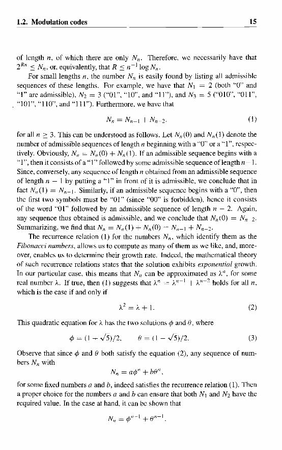
. "101", "110", and "111"). Furthermore, we have that

(1)

for all n ::: 3. This can be understood as follows. Let Nil (0) and Nil (1) denote thenumber of admissible sequences of length n beginning with a "0" or a "1", respec­tively. Obviously, Nil = NIl(O) + Nil (1). If an admissible sequence begins with a"1", then it consists of a "1" followed by some admissible sequence of length n-l.Since, conversely, any sequence of length n obtained from an admissible sequenceof length n - 1 by putting a "1" in front of it is admissible, we conclude that infact NIl(I) = Nil-I. Similarly, if an admissible sequence begins with a "0", thenthe first two symbols must be "01" (since "00" is forbidden), hence it consistsof the word "01" followed by an admissible sequence of length n - 2. Again,any sequence thus obtained is admissible, and we conclude that Nn (0) = Nn-2.

Summarizing, we find that Nn = Nn(l) + Nil (0) = NIl-I + N Il-2.

The recurrence relation (1) for the numbers Nn , which identify them as theFibonacci numbers, allows us to compute as many of them as we like, and, more­over, enables us to determine their growth rate. Indeed, the mathematical theoryof such recurrence relations states that the solution exhibits exponential growth.In our particular case, this means that Nn can be approximated as 'An, for somereal number 'A. If true, then (1) suggests that 'An = 'An- I + 'A1l -'2 holds for all n,

which is the case if and only if

This quadratic equation for 'A has the two solutions ¢ and e, where

(2)

¢ = (1 + ~)/2, e = (1- ~)/2. (3)

Observe that since ¢ and e both satisfy the equation (2), any sequence of num­bers Nn with

Nn = a¢1l + ben,

for some fixed numbers a and b, indeed satisfies the recurrence relation (1). Thena proper choice for the numbers a and b can ensure that both N I and N2 have therequired value. In the case at hand, it can be shown that

Nn = ¢n-l + ell-].

16

Since <jJ > 181, we have that Nn ~ <jJn-l, and hence that

. 10gNnlIm -- = 10g<jJ.

n--+oo n

1. Introduction

(4)

(Here the function "log" refers to the logarithm with base 2.)This last expression enables us to establish an upper bound for the coding rate

of our constraint. Indeed, from (4), it follows that

R -:::. C,

where

C = log <jJ = 0.6942· ..

is the capacity of our constraint.

1.2.3 The capacity of constraints of finite type

Consider a constrained system'c. As in the example above, we let Nn denote thenumber of constrained sequences of length n. We now define the capacity C(,c)of the constrained system ,c as

1. log N n

C(,c) = 1m--n--+oo n

(5)

provided that this limit exists. Intuitively, this quantity represents the average

amount of il!formation (in bits) carried by a bit (~fa constrained sequence. Now asimilar reasoning as in the above example shows that encoding at a rate R can onlybe possible if R -:::. C(L:) and, moreover, it suggests the possibility of encoding atrates arbitrarily close to C (,c).

What is less clear is whether this limit exists and how it could be computed.Obviously. if the constrained system consists of some arbitrary collection of se­quences. nothing much can be said, so let us restrict our attention to the morestructured type of constrained systems as encountered in practical applications.To keep things simple and to help our intuition as much as possible, we will atfirst only consider constrained systems of finite type. Recall that such a systemis described in terms of a finite collection of "forbidden subwords". (For exam­ple, the Fibonacci system discussed earlier is specified by the forbidden subword"00".) So let us assume that our constrained system ,c is specified by the finitecollection :F of forbidden subwords, and suppose that all words (patterns) in :Fconsist of at most m + 1 bits, that is, have length at most m + 1, for some in­teger m. (For the Fibonacci system, we have m = 1.) By the way, note that

1.2. Modulation codes

o

17

o

Figure 2: A presentation of the Fibonacci system.

we might as well assume that all words in :F have length m + I. Indeed, for­bidding, e.g., the word 000 is (almost) equivalent to forbidding the four words00000,00001,00010, and 00011. (This makes a difference only at the end of asequence, but does not change the behaviour of n-1log Nn for n ---+ 00.)

We are interested in how a given constrained sequence can be extended toa longer constrained sequence. Since all forbidden subwords have a length atmost m + 1, to answer this question we need only to know the last m bits of oursequence. These last m bits calTy all the necessary information and are refelTedto as the (terminal) state of the sequence. If we know the state of our sequence,we know both how it can be extended and the state of the extended sequencethat is obtained. Indeed, we could imagine the generation of a long constrainedsequence as a process where we move from state to state and generate a new bitby each transition from a state to the next state. This is a crucial image which thereader should keep in mind for what follows.

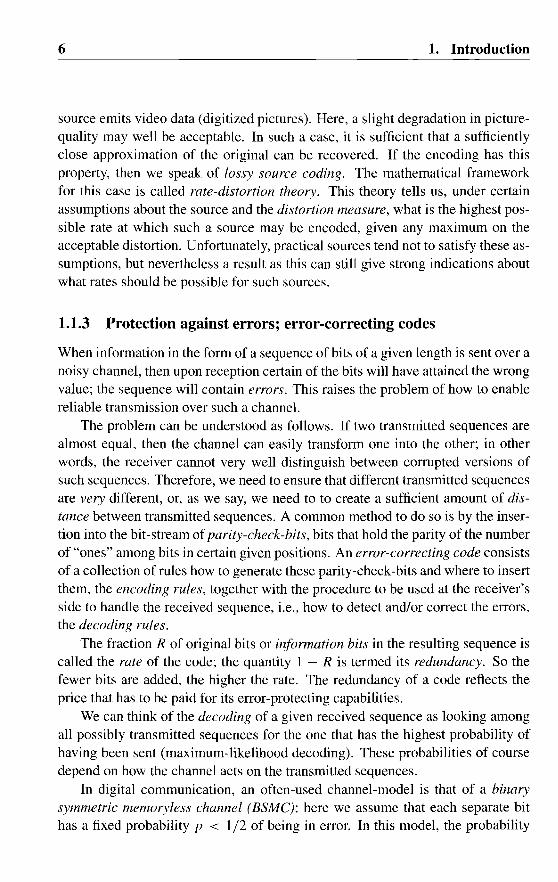
In fact we have now rediscovered an alternative description of a constrain­ed system of finite type in terms of a (labeled directed) graph. Here, a graphG = (V, A) consists of a collection V of vertices or states, and a collection Aof labeled arcs or transitions between states. We will write beg(a) and end(a) todenote the initial state and the terminal state of the transition a. Some authorsrefer to a "labeled directed graph" as defined above as a finite-state transitiondiagram or FSTD. The constrained system L(G) presented by G consists of allsequences that can be obtained by reading off the labels of a path in the graph,or, as we will say, the sequences that are generated by paths in G. (Instead of theword "path", some authors use the word "valk.)

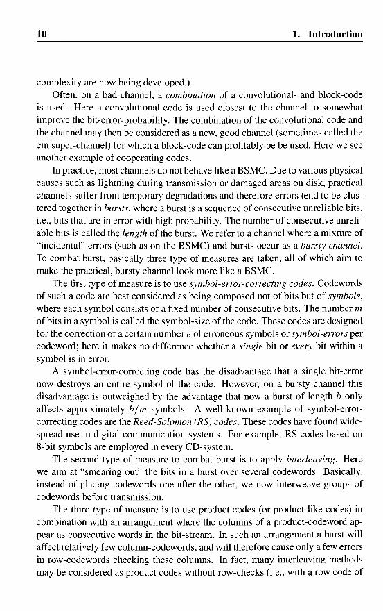
For example, the graph presenting the Fibonacci system is depicted in Fig­ure 2. It has two states, 0 and I, and three transitions. a transition from state I tostate I with label I, a transition from state I to state 0 with label 0, and a tran­sition from state 0 to state 1 with label 1. (There is no transition from state 0 tostate O. since that would allow the generation of a sequence containing the for­bidden word 00.) More general, a (d, k)-constrained system can be presented bythe graph in Figure 3. Here, we follow common practice in that the state labelindicates the number of trailing zeroes of the cOlTesponding terminal state.

18 1. Introduction

Figure 3: Presentation ofa (d, k)-constrained system.

Let us now see how such a presentation allows us to determine the numberof constrained sequences of a given length. We can consider such a sequence toconsist of the first m bits, referred to as the initial state of the sequence, followedby the bits generated by the path that has as its states the consecutive m-bit sub­words of the sequence. Note also that different paths in the graph from the sameinitial state generate different sequences. Therefore, if for n ~ m we let Nn (s)

denote the number of constrained sequences of length n with initial state s, thenfor n ~ m + 1 these numbers satisfy the recurrence relation

(6)

where the sum is over all transitions a with beg(a) = s. For example, for theFibonacci system, we obtain that

Nn(O) = Nn-l (1)

and

for n ~ 2, from which the recurrence relation (1) was obtained.As in the case of the Fibonacci system, the mathematical theory of the type

of recurrence relations (6) shows that the number Nn = Ls Nn(s) of constrainedsequences of length n exhibits exponential growth, but in this case the theory ismuch more involved. Since the underlying ideas are crucial not only for capacitycomputations, but also for a good understanding of the field of code constructionas a whole, we will nevertheless go somewhat more into details.

It turns out that, at least for the graphs derived from finite-type constraints asexplained above, all information concerning the numbers Nn (s) can be obtainedfrom what is called the adjacency matrix of the graph. Here, the adjacency ma­trix D of a graph G is a square array of non-negative numbers, with both rowsand columns indexed by the states of G, where the number D(s. t) in the sthrow and tth column counts the number of transitions in G from state s to state t.Readers familiar with matrix theory will have no difficulty verifying that then the(s, t)-entry of the nth power Dn of D in fact equals the number of paths oflength n

1.2. Modulation codes 19

in G from state s to state t. So the sum of the entries in D n actually counts thenumber of paths of length n in the graph.

We can use the adjacency matrix to investigate the recurrence relations (6)as follows. Let li?> denote the number of paths in G of length n starting in s,or, equivalently, the number of sequences generated by such paths, and let lien)

denote the vector with as its entries the numbers li;n). As we observed earlier, wehave that

(7)

hence from (6) we obtain that

(8)

for all n :::: 1. (By the way, it is also easy to see directly that this recurrencerelation holds.) Note that, as a consequence of (7) and an earlier observation,the number N n actually grows like the sum of the entries of powers D n of theadjacency matrix D! Using the relation (8) repeatedly, we can express the vectorsli(n), n > m, in terms of the vector Jr(m) as

(9)

At this point, we need a result from the classical Perron-Frobenius theory fornon-negative matrices (note that our adjacency matrix D is ofthis type). The saidresult states that the largest real ("Perron-Frobenius") eigenvalue A = AD of Dhas the property that the matrices (A ~l D)n tend to a limit if n tends to infinity,see e.g. [47], [43]. Now divide both sides of the equation (9) by An, let n tend toinfinity, and then use this result. If we do so, we find that for n ---+ 00 the vectorsA-nJr(n) tend to some limit vector Jr. Hence there are (non-negative) constants Jrs ,

S E V, such thatlim Nn(S)/An = Jrs .n~,CXl

(In fact, using (8) it can be shown that the vector Jr is a right-eigenvector of thematrix D, that is, Ali = DJr.) This result is just what is needed, and implies thatthe capacity C(L) of the constrained system L(G) presented by G is given by

. 10gNnC(L) = hm -- = log AD.

n---+oo n

This expression enables us to actually calculate the capacity of any given con­strained system of finite type. Indeed, the Perron-Frobenius eigenvalue can becomputed, e.g., as the largest real zero of the characteristic polynomial XD(A) =det(Al - D) of the matrix.

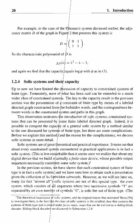
1. Introduction

For example, in the case of the F bonacci system discussed earlier, the adja­cency matrix D of the graph in Figur 2 that presents this system is

Di(~: ). /

So the characteristic polynomial of p is I I

XDO,j ;,.1 ), 1, /

and again we find that the capacity equals log¢ with ¢ as in (3).

1.2.4 Sofie systems and thei capacity

Up to now we have limited the dscussion of capacity to constrained systems of I

finite type. Fortunately, most of Iwhat has been said can be extended to a much wider class of constrained systel~s. The key to the capacity result in the previous section was the presentation of ~ constraint of finite type by means of a labeled directed graph constructed from the forbidden words, and the correspondence be-

I

tween words in the constrained ~ystem and paths in this graph. This observation motivates ~le introduction of sofie systems, constrained sys­

tems that can be presented by ~ome finite labeled directed graph. Indeed, it is possible to compute the capa*i y of a general sofic system by a method similar to the one discussed for syste s of finite type, but there are some complications. Before we explain this method (and the reason for the complications), we discuss sofic systems in more detail. I

Sofic systems are of great treoretical and practical importance. It turns out that about every constrained systep1 encountered in practical applications is in fact a sofic system. (This is less remlarkable than it seems once we realize that about any

I digital device that we build is/actually a./inite-state device, whose possible output

I sequences necessarily consti~ute some sofic system.)!

In the previous section, .,ye have shown that each constrained system of finite type is in fact a sofic systeml and we have seen how to obtain such a presentation given the collection of its fqrbidden subwords. However, as we will see later on, many (in fact "almost all")i sofic systems are not of this special type. the even system, which consists of ~1I sequences where two successive symbols HI" are separated by an even number of symbols "0", is sofic but not of finite type. (The

I IThe theoretical importancejf sofic systems. and the original reason that motivated Weiss 154]

to investigate them, is the fact t at the class of sofic systems is the smallest class that contains the systems of finite type and is clo ed underfclctor maps, maps that can be realized as a sliding-block decoder. Sliding-block decoder. are discussed in Subsection 1.2.6.

I

1.2. Modulation codes 21

{J:(}

Figure 4: Two presentations of the full system.

forbidden subwords are precisely the words of the form 102n+J 1 with n :::: 0.) We leave it to the reader to find a presentation of this sofie system. (Hint: there are two "ending-conditions" of a constrained sequence, namely ending in an even (possibly nUll) or in an odd number of zeroes.)

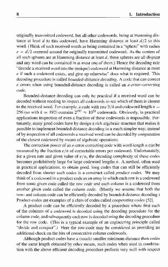
It is important to realize that a given sofie system has many different presen­tations. (Indeed, several code construction methods actually amount to finding a "suitable" presentation.) For example, the full system consisting of all binary se­quences can be presented by both graphs in Figure 4 (and by infinitely other ones). Fortunately, it can be shown constructively that each sofie system has a unique minimal deterministic presentation, called the Fisher cover or the Shannon cover of the system. That is, among all deterministic presentations, presentations where in each state the outgoing transitions from that state carry distinct labels, there is a unique one with the minimal number of states.

The Fisher cover of a sofie system is important: it can be constructed from any presentation of the sofie system; moreover, many properties of a sofie system can be read off directly from its Fisher cover. (We will mention one such property later in this section.)

To explain how the Fisher cover can be obtained, we first have to discuss an important means to reduce the number of states in a presentation, an operation called state merging. This works as follows. Suppose that the outgoing transitions in two given states can be paired off in such a way that the two transitions in each of the pairs carry the same label and end in the same state. Then these states have the same follower set, where the follower set of a state is the collection of sequences that can be generated by paths leaving this state. So from the point-of­view of sequence generation, these two states accomplish the same, hence they can as well be combined, or merged as it is usually called, into a single state. (Note that if the original presentation is deterministic, then the resulting presentation will again be deterministic.)

22 1. Introduction

To construct the Fisher cover fro a given presentation, we proceed as fol­lows. First, we transform the prese tation into one that is deterministic. This can be achieved, e.g., by using a va~ant of the well-known subset construction for finite automata (see for example/ [28], [29]), or by state-splitting (see Sub­section 1.2.8). Then we reduce the ~umber of states in the presentation by state merging. This process of merging s~ates is repeated until no further merging is possible. It can be shown that the r~sulting presentation, the Fisher cover, does not depend on the order in which thelmerging was carried out, and that, moreover, no deterministic presentation of the $ystem can have fewer states; moreover, such a presentation must be equal to the F~sher cover if it has the same number of states. (For further details on this construcqon, we refer to [38].)

Readers familiar with automata iheory will recognize the parallel with regular languages, the class of languages gdnerated by finite automata. Here also, a given regular language can be generated b~ many different finite automata among which there is a unique minimal determini~tic one. In fact, the resemblance is more than superficial; a sofic system is in faqt a regular language, and the construction of the Fisher cover for a sofic system arallels the construction of its minimal finite deterministic automaton. 2

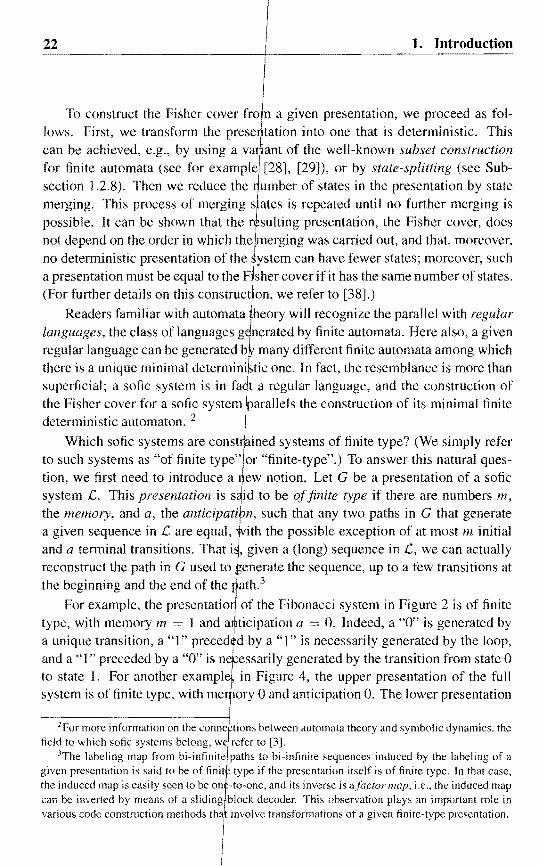
Which sofic systems are const ined systems of finite type? (We simply refer to such systems as "of finite type" or "finite-type".) To answer this natural ques­tion, we first need to introduce a ew notion. Let G be a presentation of a sofic system C. This presentation is s id to be of finite type if there are numbers m, the memory, and a, the anticipatifm, such that any two paths in G that generate a given sequence in C are equal, with the possible exception of at most m initial and a terminal transitions. That i~, given a (long) sequence in C, we can actually reconstruct the path in G used to senerate the sequence, up to a few transitions at the beginning and the end of the gath.3

For example, the presentatiod of the Fibonacci system in Figure 2 is of finite type, with memory m = 1 and a,ticipation a = O. Indeed, a "0" is generated by a unique transition, a "1" preced¢d by a "I" is necessarily generated by the loop, and a "I" preceded by a "0" is n¢essarilY generated by the transition from state 0 to state 1. For another example( in Figure 4, the upper presentation of the full system is of finite type, with me+ory 0 and anticipation O. The lower presentation

I 2For more information on the conne

l tions between automata theory and symbolic dynamics. the

field to which sofic systems belong, w refer to [3]. 3The labeling map from bi-infinite paths to bi-infinite sequences induced by the labeling of a

given presentation is said to be of finit type if the presentation itself is of finite type. In that case, the induced map is easily seen to be on -to-one, and its inverse is alactol' map, Le., the induced map can be inverted by means of a sliding block decoder. This observation plays an important role in various code construction methods that! involve transformations of a given finite-type presentation.

I I

1.2. Modulation codes 23

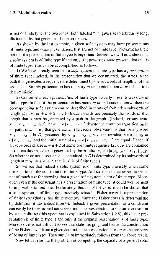
is not of finite type: the two loops (both labeled "1") give rise to arbitrarily long, distinct paths that generate all-one sequences.

As shown by the last example, a given sofie system may have presentations of finite type and other presentations that are not of finite type. Nevertheless, the notion of a presentation of finite type is important. Indeed, we will now show that a sofic system is of finite type if and only if it possesses some presentation that is of finite type. This can be accomplished as follows.

1) We have already seen that a sofie system of finite type has a presentation of finite type; indeed, in the presentation that we constructed, the states in the path that generates a sequence are determined by the subwords of length m of the sequence. So this presentation has memory m and anticipation a = 0 (i.e., it is deterministic ).

2) Conversely, each presentation of finite type actually presents a system of finite type. In fact, if the presentation has memory m and anticipation a, then the corresponding sofic system can be described in terms of forbidden subwords of length at most m + a + 2; the forbidden words are precisely the words of that length that cannot be generated by a path in the graph. (Indeed, for any word x = X-m ... Xa in C, let a = a[x_m ... xa] denote the common transition ao in all paths a-m ... aa that generate x. The crucial observation is that for any word X-m " 'Xa+l in C, generated by a-m ·· ·aa+l, say, the terminal state of ao a[x-m ... xa] and the initial state of al a[X-m+l ... Xa+l] are equal. Hence, if all subwords of size m + a + 2 of some bi-infinite sequence {X/I }/IEZ are contained in C, then this sequence is generated by the bi-infinite path {a[xn - m ... Xn+a]}nEZ, So whether or not a sequence is contained in C is determined by its subwords of length at most m + a + 2, that is, C is of finite type.)

So we see that indeed a sofic system is of finite type precisely when some presentation of the constraint is of finite type. At first, this characterization seems not of much use for showing that a given sofic system is not of finite type. More­over, even if the constraint has a presentation of finite type, it could well be next to impossible to find one. Fortunately, this is not the case: it can be shown that a sofic system is of finite type precisely when its Fisher cover is a presentation of finite type (that is, has finite memory; since the Fisher cover is deterministic by definition it has anticipation 0). Indeed, a given presentation of a constraint can easily be transformed into a deterministic presentation for the same constraint by state-splitting (this operation is explained in Subsection 1.2.8); this latter pre­sentation is of finite type if and only if the original presentation is of finite type. Moreover, it is not difficult to see that state-merging, and hence the construction of the Fisher cover from a given deterministic presentation, preserves the property of being of finite type. Then our claim immediately follows from the above result.

Now let us return to the problem of computing the capacity of a general sofic

24 1. Introduction

system, i.e., the evaluation of the limit in (5).4 Let us recall how this was donefor systems of finite type. We first derived a (deterministic) presentation for thesystem, and this gave us a recurrence relation for the numbers Nn(s) of sequencesin the system with initial state s. Then we used the adjacency matrix D of thegraph to establish that the sum Nn of these numbers grows like the number of pathsof length n n the graph, that is, as the sum of the entries of D n . Since accordingto Perron-Frobenius theory this sum grows exponentially in AD, the largest realeigenvalue of D, the same holds for Nn , which, according to the definition of thecapacity, establishes that the capacity equals log AD.

We can do the same thing for a general sofie system, using the adjacencymatrix of some presentation of the system, but there is a problem. As observedearlier, the entry Dn(s, t) of the nth power Dn ofthe matrix D actually counts thenumber of paths of length n from state s to state t in the graph that presents thesystem, and like before the sum of these entries, that is, the total number of pathsof length n in the graph, grows exponentially in AD.

However, it may well happen that many of these paths generate the same se­quence, and if so it may well happen that the number of sequences of length n

is significantly smaller than the number of paths of that length, thus turning ourcomputations into "nonsense". (For a most dramatic example, imagine that alllabels in the graph are equal to "0". Then the sofie system presented by the graphconsists of the sequences on, n ~ 0, only, so the capacity is zero, but the PelTon­Frobenius eigenvalue of the corresponding adjacency matrix could be anything!)

By the way, note that this problem cannot occur if the presentation is of finitetype, but we have seen before that the only sofie systems possessing such a pre­sentation are those of finite type! Fortunately, to avoid this problem it is sufficientthat the presentation is deterministic. (Note that the presentation for a constraintof finite type as derived earlier is deterministic!) Indeed, in that case all paths oflength n that begin in a given state generate different sequences, and this is suf­ficient to conclude that the exponential growth rate of the number of constrainedsequences of length n and the number of paths in the graph of length n are equal.

Summarizing the above, we conclude that the capacity of a sofie system pre­sented by a given graph can be computed as follows. First, we construct a de­terministic presentation for the system. This can be done by splitting states until

4The fact that this limit exists immediately follows from Feteke's Lemma ([ II ], see also [46]): ifthe non-negative numbers an are such that am+n ::: am +al/. for all n, m ~ O. then a* = limn --+ 00 aI/Inexists and a* ::: anin for all n. Indeed, if Nn is the number of sequences of length n contained in asubword-closed constrained system L, then obviously Nm+n ::: Nm Nn • hence an application of thisLemma with an = log Nil shows that such constrained systems have a well-defined capacity. Notethat sofic systems are subword-closed; in fact, the sofic systems are precisely the subword-closedregular languages.

1.2. Modulation codes 25

the resulting presentation is deterministic. We will discuss state-splitting later.(We might even choose to construct the Fisher cover, an attractive choice sinceit has the minimum possible number of states.) Then we establish the adjacencymatrix D of the deterministic graph thus obtained, compute its Perron-Frobeniuseigenvalue AD, and obtain the capacity C of the system as C = log AD.

Sofic systems and their bi-infinite counterparts sofic shifts belong to the sub­ject of symbolic dynamics. For more information on this subject and its relationto coding theory we refer to [38] and [7]. The first of these is devoted to symbolicdynamics and modulation codes, and the second one provides some backgroundon error-correcting codes and also contains a few chapters linking symbolic dy­namics to coding theory, automata theory and system theory.

1.2.5 Encoding and encoders

An encoder for a given constrained system L is a device that transforms arbitrarybinary sequences of source bits into sequences contained in L. Commonly, theencoder is realized as a synchronous finite-state device. Such a device takes sourcesymbols, groups of p consecutive source bits, as its input, and translates these intoq-bit words called codewords, where the actual output depends on the input andpossibly on the internal state, the content of an internal memory, of the device.(Note that since an actual hardware-realization of such a device can only containa finite amount of memory, the number of internal states is necessarily finite.)The rate of such an encoder is then R = P/ q. (To stress the individual valuesof p and q we sometimes speak of a "rate p ---+ q" encoder.) Obviously, eachcodeword must itself satisfy the given constraint. Moreover, the encoder needsto ensure that the bit-stream made up of successive codewords produced by theencoder also satisfies the constraint.

In the simplest case, the encoder translates each source symbol into a uniquecorresponding codeword, according to some code table. Of course this will onlyproduce an admissible sequence if the concatenation of any number of these code­words, in any order, also satisfies the given constraint. (Here, the concatenation oftwo words a and b is the word ab consisting of the bits of the first word followedby the bits of the second word.)

For an example, let us consider again the Fibonacci system, the collectionof (0, I)-constrained sequences where the subword "00" is not allowed to occurin the sequence. A possible encoder has p = 1 and q = 2 (so the rate of this codewill be R = 1/2), and translates the source symbol "0" into the codeword "10"and the source symbol"1" into"11". It is now easily seen that any succession ofthe codewords "10" and "11" will indeed never contain the forbidden pattern "00".This simple code is called the Frequency Modulation (FM) or bi-phase code.

26 1. Introduction

Note that the original source sequence can easily be obtained from the en­coded sequence, namely by dropping every other bit from the encoded sequence.So decoding is possible. However, note also that, in practice, correct decoding re­quires some sort of synchronization between encoder and decoder. Indeed, practi­cal decoders dispose, at each time instant, of only a small part of the entire streamof channel bits. Consequently, there are essentially two ways to group the avail­able bits into codewords and the decoder needs to know which way to choose. Wewill discuss synchronization later on.

Earlier we computed the capacity C of this constraint and we found that C =

0.6942 .... So the efficiency R/C of this code is approximately 0.72. So althoughthis code is very simple, its rate is far from optimal. It would be much better tohave a code rate of, say, 2/3, for an efficiency of about 0.96.

So let us try to devise, in a similar way, a code with p = 2 and q = 3. Theavailable codewords of length three are

010. 011, 101, 110, 111,

since all other words of length three contain the forbidden pattern "00". Thereare four source symbols (namely 00, 01, 10, and 11), so we need to pick fourcode words for our translation table. Unfortunately, whatever four codewords wechoose, among them there will always be one ending in a "0" and one beginningwith a "0", and then these two cannot be concatenated without violating our con­straint. We could use the same idea, but then with larger values of p and q forwhich p / q = 2/3. In fact, a moment of reflection reveals that in order to succeedwe need a collection of 2P code words of length q, all of which begin with a "1"(or, equivalently, all of which end with a "1"). The number N q (1) = Nq-l of suchcodewords can be computed from (1), and if we do so we find that the smallest pand q that work are p = 12, q = 18. But then our encoder would need a enor­mous encoding table to memorize all translations, and would therefore require toomuch hardware.

The previous code construction method can be considered as a simple exampleof the principal-state method of Franaszek. Here, we search for a collection ofstates, referred to as principal states, in a presentation of the constraint, withthe propelty that for each of these principal states there are "sufficiently many"encoding paths beginning at this state and ending in another principal state. Inour case, the set of principal states consists of the single state "1".

As this example shows, we need a more subtle approach to the design of effi­cient codes which possess simple encoders. Nevertheless, the idea in this examplecan be used to show that, for a given sofic system with capacity C, any encodingrate R = P/ q ::: C can be achieved, provided that we allow arbitrarily large val­ues of p and q. However, to obtain simple, easy-to-build encoders, we need to

1.2. Modulation codes 27

keep p and q small. (Very recently, some progress has been made [34, 35] whichshows that, even if p and q are large, systematic encoding may still be possibleby using a smart variant of enumerative encoding [8]. Nevertheless, this new ap­proach has its own problems and the above statement that p and q should betterbe small is a reasonable approximation of the truth.)

To do better, we need the encoder to base its encoding decision on more thana single source symbol input alone. For example, consider again the design of arate-2/3 encoder for the Fibonacci system with p = 2 and q = 3. We will denotethe source symbols 00,01, 10, and 11 by 0, 1,2, and 3, respectively. Suppose thatthe encoder tries to use the following simple encoding rule:

0-+011, 1 -+ 101, 2 -+ 110, 3-+111. (10)

This works fine except when the encoder input is a "2" followed by a "0", whichproduces the word 110.011 in the encoder output. However, this problem canbe eliminated provided that we allow the encoder a "second stage" to modify itsinitial outputs, by replacing, from left to right, each occurrence in the output ofthe words 110.011 and 110.110 by the words 010.101 and 010.111, respectively.(Here, the second substitution is required to avoid problems when the input se­quence contains "220".)

Note that decoding of this code is possible: the decoder decodes the codeword010 into the source symbol "2", and uses the rules (10) to decode the other code­words, except when the previous codeword was 010, in which case 101 and 111are decoded as "0" and "2", respectively. This encoder can be realized as a finite­state device that encodes with an encoding delay of one source symbol. (Thisdelay is needed to "look ahead" to the next source symbol.) The "state" of theencoder memorizes the previous source symbol and whether or not a substitutionis in progress.

The above encoding method is sometimes called the substitution method. Asimilar, but more complicated example of the substitution method is the rate-2/3(1, 7)-code in [36]. This method can be interpreted as a principal-state methodwhere we allow the encoding paths to have different lengths. In Subsection 1.2.8we will discuss various other code construction methods. Some of these methodsare best understood as constructing look-ahead encoders for the constraint, analternative encoder description that will be discussed at that time.

1.2.6 Decoding and decoders

The use of the word "code" implies that it should be possible to recover or decodethe original sequence of p-bit source symbols from the corresponding sequenceof q-bit codewords. However, in practice a stronger requirement is needed. As can

28 1. ImI'''' <!.

bits '--.

I •

I I I I I I

Sliding Decoder Direction~ Logic

I I I I I ,

I I I I

p bits I I I

Figure 5: A sliding-block decoder.

be seen from Figure], the encoded sequence is directly transmitted over the chan­nel, and due to the occurrence of noise on the thannel the received sequence may contain errors. Surely, we do not wish that oQe (or a few) errors in the received sequence could cause the decoder to produce ~n unlimited number of errors in the decoded sequence! Therefore, we commonly rbquire that the modulation code can be decoded by a sliding-block decoder. A sliding-block decoder for a rate p -+ q encoder takes (a sequence of) q-bit words Yn as its input, and produces a sequence of p-bit symbols XI1 as its output, where each loutput symbol XI1 only depends on a corresponding sequence Yn-m, ... , Yn+a of tv = m + 1 + a consecutive inputs, for some fixed numbers m and a, m < a. We will refer to the number w as the window size of the decoder. (The numbers m and a are referred to as the memory and anticipation of the decoder.) The name "~liding-block decoder" refers to the image of the decoder sliding a "window" of ~idth w over the sequence to be de-

I

coded. (Refer to Figure 5.) Note that an error ~n the encoded sequence will cause at most w symbol errors in the original sequ~nce. So the error propagation, the amount of erroneous bits in the decoder outpilit caused by a single input error, is limited to at most wp bits.

The window-size of the decoder is an iml?ortant parameter of a code: it pro­vides an upper bound on the error propagatiOl} of the code, and also gives a good indication of the size of the decoder, the amount of hardware necessary to imple­ment the decoder. (That is, it provides an upper bound on the complexity of the decoding operation.) Indeed, often the size of,the decoder is more important than the size of the encoder; think for example of dJvices such as a compact disc player which only need to handle previously stored Jr transmitted data and therefore do not need to have an encoder on board! !

1.2. Modulation codes 29

Codes with a window-size of one codeword are called block-decodable. For such codes, decoding a given codeword or block can be achieved without any knowledge of preceding or succeeding codewords. In many present-day appli­cations, modulation codes are used in combination with symbol-error-correcting codes based on Reed-Solomon codes over some finite field GF(2P). In that situ­ation, the use of a rate p -+ q block-decodable modulation code becomes espe­cially attractive, since then a channel-bit error affects at most one p-bit symbol of a Reed-Solomon codeword. Note that this cannot be guaranteed if a non-block­decodable code is used, even if the window-size of the code is smaller than q bits.

We have already met some block-decodable codes: the rather trivial rate 1 -+

2 FM code and a possible rate 12 -+ 18 code for the Fibonacci system of (0, 1)­constrained sequences in subsection 1.2.5. (Note that the arguments given there actually show that any rate-2/3 block-decodable code for this system must have codewords of length q 2: 18.) Another well-known example of a block-decodable code is the Modified Frequency Modulation (MFM) or Miller code. This is a rate I -+ 2 (1, 3)-code which, like the FM code, encodes by inserting a merging bit between each two consecutive source bits. Here, the merging bit is set to "0" except when both surrounding bits are "0", in which case it is set to "I". (For the FM code, the merging bit is always set to "1 ".) The MFM code is indeed block­decodable: decoding amounts to dropping each second bit, which can be realized as an operation on 2-bit codewords.

The use of merging bits is a well-established technique for constructing block­decodable (d, k)-codes. They are often employed in combination with (dklr)­sequences, that is, (d, k )-constrained sequences in which the number of leading and trailing zeroes is restricted to be at most I and r respectively [4]. Here, p-bit source symbols are uniquely translated into (dklr)-sequences of a fixed length q', and a fixed number of q q' merging bits, chosen according to a set of merging rules, is employed to ensure that the resulting bit stream is a valid (d, k)-sequence. For some recent information on these methods, we refer to [53]. A similar idea is used in [33] to construct almost-block-decodable (d, k) codes.

As exemplified by the rate-2/3 Fibonacci code, block-decodable (d, k)-codes with a prescribed rate may require a large codeword size. In these cases, it is often possible to do much better for the corresponding (d, k) RLL constraint, provided that we a]]ow the encoder to employ (one symbol) look-ahead. This recent, rather surprising insight is explained in detail in [32].

1.2.7 Synchronization

For correct functioning, the decoder needs to properly group the bits in the en­coded sequence into its composing q-bit codewords. Therefore some form of syn-

30 1. Introduction

chronization between encoder and decoder has to be established. We will brieflydiscuss some means to do so.

Usually, at the encoder side the p-bit source symbols are grouped into frames,each consisting of afixed number of source symbols. (Usually, a frame is in factmade up from a fixed number of error-correcting codewords.) The beginning ofeach frame will be signalled by the occurrence of a special pattern called the frameheader. Commonly, the frame header is required to be unique, that is, it shouldnot occur at any other locations in the sequence. The use of frames and uniqueframe headers will enable the decoder to recognize the beginning of each frameand thus to establish the desired synchronization.

Often, we require that the header itself, and possibly even the entire bit-stream,also satisfies the imposed constraint. To achieve this, one commonly employs inci­dental constraints. As the name suggests, these are certain patterns that do satisfythe constraint but do not occur as a subword in the output of the encoder duringnormal operation. If we think of the encoding process of following certain en­coding paths in a presentation of the constraint, then the incidental constraints areassociated with paths that are never used for encoding purposes.

As an example, consider again the rate 2 --+ 3 code for the Fibonacci sys­tem constructed in Subsection 1.2.5. It is not difficult to verify that the encoderoutput never contains the pattern 0.110. We can profit from this fact to design aunique frame header: for example, we could choose as a header the codeword se­quence 110.110.101, which possesses the added advantage that it can be insertedanywhere in the codeword stream without violating our constraint, to signal thebeginning of each frame.

The presence of noise on the channel may cause bit-errors in a frame header,which may cause the decoder to occasionally miss a header. This problem isusually dealth with by using a PLL-like device similar to the one employed by thereceiver to avoid clock-drift of its internal bit-clock.

1.2.8 Code-construction methods

What we would like is a systematic method to design a sliding-block decodablecode for a given constrained system £, presented by some deterministic graphG = (V, A), say, at a given rate p ---+ q. Over the years, a great many of suchconstruction methods have been devised. We will review a large number of themhere; along the way, we will meet some techniques that we already encounteredearlier. Almost all of these methods employ approximate eigenvectors to guidethe construction. We will first explain what these are and, especially, why thisis so. To this end, consider a code meeting our requirements. We will assumethat an encoder for our code takes p-bit symbols as its input, and produces q-bit

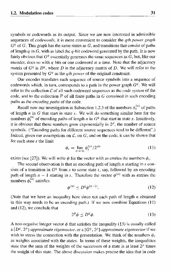
1.2. Modulation codes 31

symbols or codewords as its output. Since we are now interested in admissiblesequences of codewords, it is more convenient to consider the qth power graph

Gq of G. This graph has the same states as G, and transitions that consist of pathsof length q in G, with as label the q-bit codeword generated by the path. It is nowfairly obvious that Gq essentially generates the same sequences as G, but, like ourencoder, does so with q bits or one codeword at a time. Note that the adjacencymatrix of Gq is Dq, where D is the adjacency matrix of D. We will refer to thesystem presented by Gq as the qth power of the original constraint.

Our encoder translates each sequence of source symbols into a sequence ofcodewords which, in turn, corresponds to a path in the power graph Gq. We willrefer to the collection C of all such codeword sequences as the code system of thecode, and to the collection P of all finite paths in G contained in such encodingpaths as the encoding paths of the code.

Recall now our investigation in Subsection 1.2.3 of the numbers rr}n) of pathsof length n in G that start in state s. We will do something similar here for thenumbers <p~n) of encoding paths of length n in Gq that start in state s. Intuitively,it is obvious that these numbers grow exponentially in 2P , the number of sourcesymbols. ("Encoding paths for different source sequences tend to be different".)Indeed, given our assumptions on £, on G, and on the code, it can be shown thatfor each state s the limit

(11)

exists (see [27]). We will write <p for the vector with as entries the numbers <Ps.The second observation is that an encoding path of length n starting in s con­

sists of a transition in Gq from s to some state t, say, followed by an encodingpath of length n - 1 starting in t. Therefore the vector <p(n) with as entries thenumbers <pln ) satisfies

(12)

(Note that we have an inequality here since not each path of length n obtainedin this way needs to be an encoding path.) If we now combine Equations (11)

and (12), we conclude that

(13)

A non-negative integer vector <p that satisfies the inequality (13) is usually calleda [Dq , 2P ]-approximate eigenvector, or a [Gq , 2P ]-approximate eigenvector if wewish to stress the connection with the presentation. We think of the numbers <Psas weights associated with the states. In terms of these weights, the inequalitiesstate that the sum of the weights of the successors of a state is at least 2P timesthe weight of this state. The above discussion makes precise the idea that in code

32 1. Introduction

construction, these weights are indicators for the relative encoding power fromthe states. This idea will be further illustrated by some of our later examples.

Approximate eigenvectors were first introduced by Franaszek. In a series ofpioneering papers [13], [14], [15], [16], [17], he systematically employed approx­imate eigenvectors to develop a number of code construction methods. For ex­ample, the principal-state method already mentioned is based on the observationthat the existence of a binary (0, I-valued) [Dq, 2P ]-approximate eigenvector isequivalent to the existence of a collection of states, the principal states, with theproperty that from each principal state there can be found at least 21' distinct tran­sitions in Gq, that is, paths of length q in G, that end in another principal state. (Tosee this, let the principal states correspond to the states with approximate eigen­vector-weight one, and now recall that the (s, t)-entry of Dq counts the numberof paths of length q from s to t.)

The collection of paths between the principal states immediately allows theconstruction of a rate p ---+ q encoder. In each principal state, the 21' possiblesource symbols are assigned to q-bit codeword labels of the paths leaving thisstate. Then the encoder uses, e.g., an encoding table in each principal state to dothe translation. (So the encoder does not need to employ look-ahead.) Usually,the encoding tables are implemented by using enumerative methods (see [8], [30].

Here, the encoding moves from one principal state to another, and indeedavoids the states with weight zero in Gq. We propose to call such codes fixed­

length principal-state codes.

If the constraint is of finite type, then any assignment of source symbols tocodewords will lead to a sliding-block decodable code: in that case, the sequenceof principal states traversed by the encoder can be reconstructed from the sequenceof codewords. However, it would of course be preferable to assign afixed sourcesymbol to each codeword, thus making the code block-decodable, and if the con­straint is not of finite type, this is almost a requirement. In general, finding sucha source-to-codeword assignment is difficult (in fact, deciding whether such anassignment exists is an NP-complete problem), but in most cases that arise inpractice this can be done. The possible remaining freedom in choosing the as­signments can be used to optimize other aspects of the code (see, e.g., the designof an 8b lOb channel code in [30]).

The method of using merging bits as discussed in Subsection 1.2.6 presents analternative approach to this labeling problem. Here, we consider only codewordsthat consist of some merging bits followed by a (fixed-length) (dklr )-sequence,and we assign source symbols to the (dklr )-sequences. This replaces the labelingproblem by the problem of assuring that in each principal state sufficiently manytransitions with codeword labels of this .<,pecial form are present. The optimalselection of principal states for (d, k) block-codes has been determined in [19].

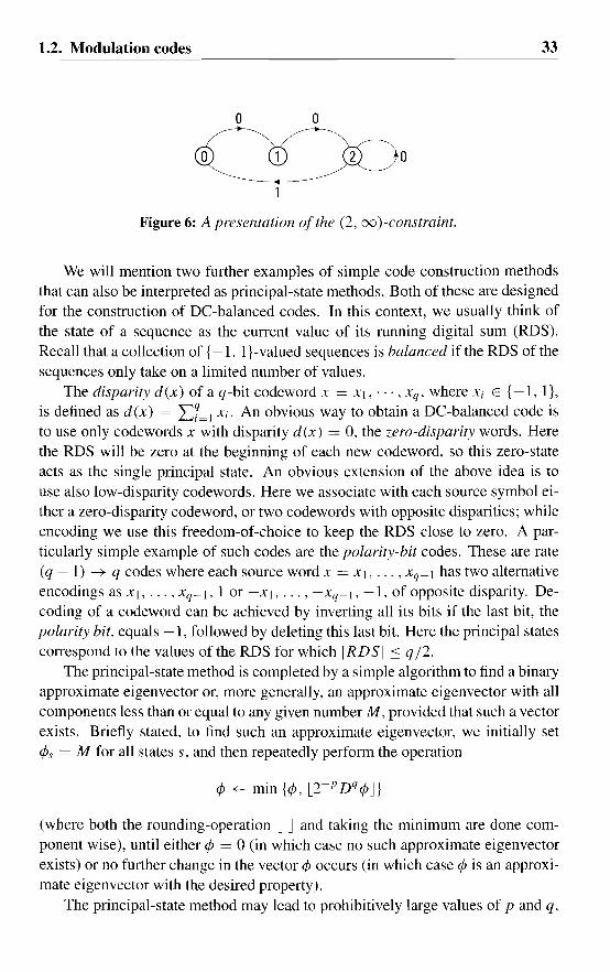
1.2. Modulation codes

o

o o

o

33

Figure 6: A presentation of the (2, 00 )-constraint.

We will mention two further examples of simple code construction methodsthat can also be interpreted as principal-state methods. Both of these are designedfor the construction of DC-balanced codes. In this context, we usually think ofthe state of a sequence as the current value of its running digital sum (RDS).Recall that a collection of {-I, 1}-valued sequences is balanced if the RDS of thesequences only take on a limited number of values.

The disparity d(x) of a q-bit codeword x = XI, ... , xq , where Xi E {-I, I},is defined as d(x) = "L;=I Xi. An obvious way to obtain a DC-balanced code isto use only codewords x with disparity d (x) = 0, the zero-disparity words. Herethe RDS will be zero at the beginning of each new codeword, so this zero-stateacts as the single principal state. An obvious extension of the above idea is touse also low-disparity codewords. Here we associate with each source symbol ei­ther a zero-disparity codeword, or two codewords with opposite disparities; whileencoding we use this freedom-of-choice to keep the RDS close to zero. A par­ticularly simple example of such codes are the polarity-bit codes. These are rate(q - 1) --+ q codes where each source word x = XI, ... , Xq-l has two alternativeencodings as Xl, ... , Xq-l, 1 or -XI, ... , - Xq-l , -1, of opposite disparity. De­coding of a codeword can be achieved by inverting all its bits if the last bit, thepolarity bit, equals -1, followed by deleting this last bit. Here the principal statescorrespond to the values of the RDS for which IRDSI ~ q /2.

The principal-state method is completed by a simple algorithm to find a binaryapproximate eigenvector or, more generally, an approximate eigenvector with allcomponents less than or equal to any given number M, provided that such a vectorexists. Briefly stated, to find such an approximate eigenvector, we initially setcPs = M for all states s, and then repeatedly perform the operation

(where both the rounding-operation LJ and taking the minimum are done com­ponent wise), until either cP = 0 (in which case no such approximate eigenvectorexists) or no further change in the vector cP occurs (in which case cP is an approxi­mate eigenvector with the desired property).

The principal-state method may lead to prohibitively large values of p and q.

34

00

00

01 10

01

00

1. Introduction

Figure 7: A presentation of G 2.

0/00

[0] 0

0/00

1(0)/01

Figure 8: A look-ahead encoder.

For example, the minimum codeword length of a fixed-length principal-state rate­2/3 (1, 7)-code and a rate-l 12 (2, 7)-code are 33 and 34, respectively. Sometimesthis problem can be avoided if we allow the coding paths between principal statesto have varying lengths. As an example, we consider the design of a rate-I/2(2, oo)-code. (The forbidden subwords are given by "11" and "101".) The min­imum codeword length of a fixed-length rate-1/2 code for this constraint is 14(see, e.g., [30]). The constraint can be presented by a three-state graph G withstates named 0, 1, and 2, see Figure 6. Here, sequences ending in state 0 or 1 haveprecisely 0 or 1 trailing zeroes, respectively, and a sequence ending in state 2 hasat least 2 trailing zeroes. The 2nd power graph G 2 of G needed in the constructionof a rate 1 ---+ 2 code is depicted in Figure 7. The vector cP which has cPo = cPl = 1and cP2 = 2 can be seen to be a [G 2 , 2]-approximate eigenvector.

Let the set of principal states consist of the single state 2. Now consider thepossible encoding paths, that is, paths in G2 starting and ending in state 2. Byinspection of G 2 , we obtain the three paths

2~2, 2~ I~2,

from which a code can now be designed. The encoding rules are specified as

o ---+

10 ---+

11 ---+

00

01.00

10.00

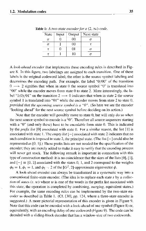
1.2. Modulation codes

Table 1: A two-state encoder for a (2, 00 )-code.

State Input Output Next state

0- 0 00 0-

0- 1 00 r

r ° 01 0-

r 1 10 0-

3S

A look-ahead encoder that implements these encoding rules is described in Fig­ure 8. In this figure, two labelings are assigned to each transition. One of theselabels is the original codeword label; the other is the source symbol labeling anddetermines the encoding path. For example, the label "0/00" of the transitiono -----+ 2 signifies that when in state 0 the source symbol "0" is translated into"00" while the encoder moves from state °to state 2. More interestingly, the la­bel "1(0)/01" on the transition 2 -----+ °indicates that when in state 2 the sourcesymbol 1 is translated into "01" while the encoder moves from state 2 to state 0,provided that the upcoming source symbol is a "0". (So here we see the encoder"looking ahead" for the next source symbol before deciding on its action.)

Note that the encoder will possibly move to state 0, but will only do so whenthe next source symbol to encode is a "0". Therefore all source sequences startingwith a "0" (and only these) have to be encodable form state O. This is indicatedby the prefix list [0] associated with state 0. For a similar reason, the list [1] isassociated with state 1. The empty list [- ] associated with state 2 indicates that nosuch condition is imposed in state 2, the principal state. (The list [- ] could also berepresented as [0, 1].) These prefix lists are not needed for the specification of theencoder; they are merely added to make it easy to verify that the encoding processwill never get stuck. The following remark is important in connection with thistype of construction method: it is no coincidence that the sizes ofthe lists [0], [1],and [-] == [0, 1] associated with the states 0, 1, and 2 correspond to the weights

4>0 = 1,4>1 = 1, and 4>2 = 2 of the [G 2, 2]-approximate eigenvector 4>.

A look-ahead encoder can always be transformed in a systematic way into aconventional finite-state encoder. (The idea is to replace each state s by a collec­tion of states (s, w) where w is one of the words in the prefix list associated withthis state; the operation is completed by combining, merging, equivalent states.)For example, the same encoding rules can be implemented by the two-state en­coder as described in Table 1. (Cf. [30], pp. 124, where a three-state encoder issuggested.) A more pictorial representation of this encoder is given in Figure 9.Note that this code can be encoded with a look-ahead of one symbol (Figure 8) or,equivalently, with an encoding delay of one codeword (Figure 9). The code can bedecoded with a sliding-block decoder that has a window-size of two codewords.

36 1. Introduction

1/00

0/001/10

Figure 9: An alternative description of the encoder.

In general, for this method to succeed we need a (finite) collection P of pathsrr in Gq between principal states such that in each principal state s, we have that

(14)

where the sum is over all paths rr starting in s (end ending in another principalstate) and where Irr I denotes the length (number of transitions in Gq) of rr. Thiscondition, the Kraft-McMillan inequality for prefix codes (see, e.g., [9]), is nec­essary and sufficient for the existence of a prefix code (such as the source words0, 10, and 11 in the above example) with word lengths equal to the path lengths.A similar, but more complicated example of the above method is the rate-l/2(2, 7)-code in [10].

Codes for constraints of finite type found by this method are always sliding­block decodable. We propose to call such codes variable-length principal-statecodes. The substitution method encountered in Subsection 1.2.5 can be seen as aspecial case of this method.

The principal states in the above methods form a sort of "resting places" forthe encoder; here, starting from a principal state any source sequence can be en­coded (so these may serve as initial states of the encoder) and we are assured thata next such resting place is reached within a finite number of steps. However,codes of this type at a given rate p -+ q do not always exist or, if they do, they donot always provide the "simplest" possible code. The bounded-delay encodablecodes introduced by Franaszek (see also [37]) do not suffer from this drawback;indeed, in its full generality the bounded-delay method to construct such codes isuniversal. That is, each sliding-block decodable code for a constraint of finite typewith a suitable (finite-state, finite-type codeword labeling, bounded encoding de­lay) encoder can, in principle, be obtained by this method.s However, Franaszeknever succeeded in turning his method into an algorithm and he showed only muchlater [18] that this construction method is as powerful as the ACH method. This

SIn fact, more is true: in principle, any sliding-block decoder, and any encoder that is not a­priory impossible to construct by this method, can indeed be constructed. For further details, see[41 and Chapter 5, in particular Appendix B.

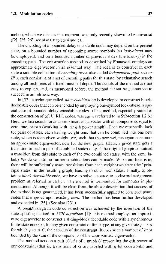
1.2. Modulation codes 37

mehod, which we discuss in a moment, was only recently shown to be universal([2], [25,26], see also Chapters 4 and 5).

The encoding of a bounded-delay encodable code may depend on the presentstate, on a bounded number of upcoming source symbols (so look-ahead maybe employed), and on a bounded number of previous states (the history) in theencoding path. The construction method as described by Franaszek employs anapproximate eigenvector in an essential way. The idea is to construct in eachstate a suitable collection of encoding trees, also called independent path sets orIP's, each consisting of a set of encoding paths for this state, by exhaustive searchamong all such trees of a fixed maximal depth. The details of the method are noteasy to explain, and, as mentioned before, the method cannot be guaranteed tosucceed in an intrinsic way.

In [32], a technique called state-combination is developed to construct block­decodable codes that can be encoded by employing one-symbol look-ahead, a spe­cial case of bounded-delay encodable codes. (This method, especially suited tothe construction of (d, k) RLL codes, was earlier referred to in Subsection 1.2.6.)Here, we first search for an approximate eigenvector with all components equal tozero, one, or two (working with the qth power graph). Then we repeatedly lookfor pairs of states, each having weight one, that can be combined into one newstate, which is then given weight two, such that the new weights again constitutean approximate eigenvector, now for the new graph. (Here, a given state gets atransition to such a pair of combined states only if the original graph containeda transition from this state to each of the two combined states, with the same la­bel.) We do so until no further combinations can be made. When our luck is in,there will be sufficiently many transitions from each weight-two state (the "prin­cipal states" in the resulting graph) leading to other such states. Finally, to ob­tain a block-decodable code, we have to solve a source-to-codeword assignmentproblem as referred to earlier. The method is well-suited for computer imple­mentations. Although it will be clear from the above description that success ofthe method is not guaranteed, it has been successfully applied to construct manycodes that improve upon existing ones. The method has been further developedand extended in [25]. (See also [23].)

A breakthrough in code construction was achieved by the invention of thestate-splitting method or ACH algorithm [I]: this method employs an approxi­mate eigenvector to construct a sliding-block decodable code with a synchronousfinite-state encoder, for any given constraint of finite type, at any given rate p ---+ qfor which p / q ::: C, the capacity of the constraint. It does so in a number of stepsbounded by the sum of the components of the approximate eigenvector.

The method acts on a pair (G, cP) of a graph G presenting the qth power ofour constraint (that is, transitions of G are labeled with q-bit codewords) and

38 1. Introduction

a [G, 2P ]-approximate eigenvector 1, and transforms this pair into another suchpair by an operation which we will call weighted state-splitting. (This operationis called ae-consistent state-splitting in [42], to which we refer for an excellentoverview of the method.) This transformation, which is guaranteed to succeed,moreover lowers at least one of the components of the approximate eigenvector,the weights, except when all non-zero weights are equal.6 So with each transfor­mation the approximate eigenvector gets "smaller", until finally a pair (G, 1) isreached where all nonzero components of 1 are equal. If that is the case, then theapproximate eigenvector-inequalities for 1 are easily seen to imply that in eachstate with a nonzero weight there are at least 2P transitions leading to other suchstates, that is, we have obtained an encoder for our constraint.

State-splitting, on which the transformation is based, is easy to understand.Think of a state as a collection of future opportunities (the transitions leaving thisstate) from which we are free to choose one. Now divide or split the state, thiscollection of opportunities, in two parts called sub-states (each having a part of theoriginal transitions). Before this splitting operation, we could move from anotherstate to this state without worrying about which opportunity (which transition) toutilise later, but now we have to choose first, before moving, from which of thetwo parts we wish to pick our next opportunity. We do not lose opportunities, butwe have to choose earlier.

In terms of the graph, this translates as follows. If s is a state, and As is thecollection of transitions from this state, then to split this state, we do the following.First, partition the set As into two non-empty parts As! and A s2 • Then, in G wereplace the state s by two states Sl and Sz (the sub-states of s), we replace eachtransition ct in part Asi , i = l, 2, by a transition from Si with the same label andending in the same state as ct, and we replace each transition fJ ending in s by twotransitions fJl and fJ2, with the same label and beginning in the same state as fJ,with fJi ending in Si, i = l, 2.

It should be evident from the preceding discussion that the new graph thusobtained presents the same sequences as the original graph. Moreover, it is notdifficult to see that if the original graph is of finite type, then the new graph isagain of finite type; the memory remains the same and the anticipation increasesby at most one. Note that if the final graph has memory m and anticipation a,then the encoder obtained from this graph by deleting all states with zero weightand assigning suitable source labels to the remaining transitions has a decodingwindow of size at most m + 1 + a.

Weighted state-splitting amounts to the same, except that now we also dis­tribute the weight of the state that is split over the sub-states (where each of

6This gives the general picture, but is not quite true. More details will be given later.

1.2. Modulation codes 39

the sub-states should receive something); moreover, we require that the result­ing weights constitute an approximate eigenvector for the new graph. Note thatthis is a local requirement which only needs to be checked for the two new states.

It is not obvious that we can always find a state for which weighted state­splitting is possible; certainly this need not be possible in each state. However,in [1] it is shown that such a state can always be found among the states with max­imum weight, provided that not all non-zero weights are equal, and an algorithmis given to find such a state.7

The ACH algorithm is again universal ([2], [26, 25], see also Chapters 4and 5). However, this method is not without drawbacks. The main problem isthe potentially large amount of freedom-of-choice afforded by the algorithm, firstin the choice of the approximate eigenvector, then both in the choice of the statesto be split and in the actual splits themselves. Different choices (almost always)lead to different codes and, by the same universality that we so much appreciatedearlier, may result in any of the (infinitely many) available codes.

As a rule-of-thumb, we usually choose the smallest possible approximate ei­genvector; a logical choice since this minimizes the a-priory upper bound on thenumber of state-splitting steps. This works very well in practice, although casesare known where this choice does not produce the best possible code [25].

Still this solves only part of the problem. Some heuristics to guide the state­splitting process have been developed (see, e.g., [42]) in order to obtain codes witha simple encoder (simple in terms of the number of encoder states), and again thisseems to work reasonably well in practice. (Methods to estimate the minimumpossible number of encoder states have been developed in [41 ].)

However. in practical applications we are often interested in codes with asmall decoding window, and the ACH algorithm provides no clues how to findsuch codes. A variant of this algorithm [25] combines ideas from the bounded­delay method of Franaszek with state-splitting to address this problem.

We will end this overview with a discussion of a very recent enumerativemethod, originally developed to design high-rate codes such as (0, k)-codes withlarge k [34, 35]. But in fact, as we will see. this method is sufficiently general todescribe many variable-length codes as well. We will first describe the methodas a means to design simple-to-implement fixed-length block-decodable codeswith a (large) codeword size q, say. Our starting point is a deterministic graphG = (V, A) presenting our constraint. We will denote the bit-label of a transitiona by L(a).

71n fact. this is only true when, after each splitting step, states with zero weight are deletedand the graph is restricted to an irreducible sink component. Note that after such an operation, theweights still constitute an approximate eigenvector for the remaining part of the graph.

40 1. Introduction

The encoding- and decoding rules of our code will be described in tenus ofnon-negative integers Nn(v), n = 0,1, ... ,q, and Nn(a), n = 1, ... , q, asso­ciated with the states v and transitions a of our presentation G. Here, all num­bers No(v) will be either zero or one, i.e.,

No(v) E {O, I}, (15)

for all states v. (These numbers will need to satisfy various other constraints thatwill be discussed later.)

Our encoder will in fact encode numbers N with 0 :s N < 2P ; the binaryrepresentation of these numbers will then correspond to the p-bit source symbols.Our encoding process will be described recursively in terms of encoding rulesfor numbers in each state. Here, the number Nn (v) will specify the interval ofnumbers that can be encoded from state v by (the n-bit label sequence of) anencoding path of length n; the first transition a of this path will lower the numberto be encoded by the amount of Nn (a). This leads to the following recursiveencoding rule: the n-bit encoding E~Il\N) of a number N, 0 :s N < Nn(v), fromstate v is given as

("the label of a, followed by an (n - I)-bit encoding"), where a is a transitionstarting in state v chosen such that

O:s N - Nn(a) < Nn-l(end(a)).

Recall that the numbers No(v) are each either zero or one. Therefore, if theencoding of a number N succeeds, then the encoding process will necessarily ter­minate with the number zero, in one of the terminal states t for which No(t) = 1.We will use T to denote the set of these terminal states. As a consequence, if theencoder has followed the path an, ... ,aI, then the number N can be recovered asthe sum

n

N = LNi(ai)i=l

(16)

of numbers subtracted at the successive transitions. So decoding is possible pro­vided that the encoding path can be retrieved from the label sequence, which ispossible if the constraint is of finite type. (If this is not the case, then in additionwe should require that paths generating identical sequences also produce identicaldecodings. A detailed discussion of that case is outside the scope of this review.)

As we observed, the encoding always terminates in a state from T. Therefore,the next encoding of a p-bit number starts in such a state; these states serve as the

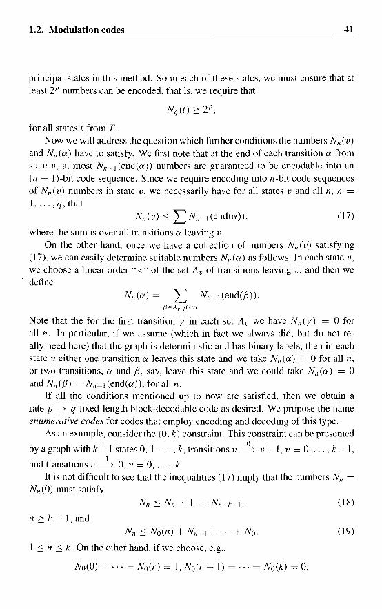
1.2. Modulation codes 41

principal states in this method. So in each of these states, we must ensure that atleast 2P numbers can be encoded, that is, we require that

for all states t from T.Now we will address the question which further conditions the numbers N n (v)

and Nn(a) have to satisfy. We first note that at the end of each transition a fromstate v, at most Nn - l (end(a)) numbers are guaranteed to be encodable into an(n - I)-bit code sequence. Since we require encoding into n-bit code sequencesof Nn(v) numbers in state v, we necessarily have for all states v and all n, n =1, ... ,q, that

Nn(v) .::=; L NIl-1 (end(a)) , (17)

where the sum is over all transitions a leaving v.On the other hand, once we have a collection of numbers Nil (v) satisfying

(17), we can easily determine suitable numbers Nn(a) as follows. In each state v,we choose a linear order"<" of the set A v of transitions leaving v, and then wedefine

Nn(a) = L Nn-I (end(,8)).;3EA".;3<a

Note that the for the first transition y in each set A v we have Nn (y) = °forall n. In particular, if we assume (which in fact we always did, but do not re­ally need here) that the graph is deterministic and has binary labels, then in eachstate v either one transition a leaves this state and we take Nil (a) = °for all n,or two transitions, a and ,8, say, leave this state and we could take Nn(a) = °and Nn (,8) = Nn - I (end(a)), for all n.

If all the conditions mentioned up to now are satisfied, then we obtain arate p ----* q fixed-length block-decodable code as desired. We propose the nameenumerative codes for codes that employ encoding and decoding of this type.

As an example, consider the (0, k) constraint. This constraint can be presented

by a graph with k+ 1 states 0,1, ... ,k, transitions v~ v + 1, v = 0, ... , k-l,

d. . I

an transltlons v ----+ 0, v = 0, ... , k.It is not difficult to see that the inequalities (17) imply that the numbers Nil =

Nn (0) must satisfy

Nn .::=; Nn-I + ... Nn-k-I,

n ::: k + 1, andNn .::=; No(n) + Nn-I + ... + No,

1 .::=; n .::=; k. On the other hand, if we choose, e.g.,

No(O) = ... = No(r) = 1, No(r + I) = ... = No(k) = 0,

(18)

(19)

42

then given numbers N n that satisfy (18) and (19), we let

for all n ~ 1, and, for states v = 1, ... , k, we let

Nn(v) = Nn-I + ... + Nn-k-!+v,

for n ~ k + 1 - v, and

Nn(v) = No(v + n) + N n- I + ... + No,

1. Introduction

for 1 :::: n :::: k - v. Then the numbers Nn(i) satisfy (17).Next, let Nn(a) = 0 if a has label ''1'' and let Nn(a) = Nn-I if a has la­

bel "0". Then all requirements are satisfied and if Nq(v) ~ 2P , v = 0, ... , r, weobtain a code with rate p ---+ q. It is also easy to see directly that the encodedsequence satisfies the k-constraint. Indeed, at any stage n we encode numbers Nwith 0 :::: N < Nn; since encoding into a "0" at stages n - 1, n - 2, ... subtractsN n- 1, N n-2, ... , the inequality (18) implies that we will do this at most k times.(More details concerning (0, k)-codes of this type can be found in [34] and [45].

An encoder and decoder for a code of this type need not necessarily be verysimple. To achieve that, we need one further idea. We have seen that any col­lection of numbers Nn(v) that satisfy both (15) and (17) can be used to devisean enumerative code. We now try to satisfy these conditions with numbers of asimple form. In particular, we will choose these numbers in such a way that, foreach fixed n, all numbers Nn(v) can be written as

(20)

witho :::: v~n) < 2/11.

Here m will be a fixed number determined by the desired implementation com­plexity. Note that now both the encoding- and decoding operations can be imple­mented as addition or subtraction on numbers represented by m+maxn(en - en-dbits, provided that we implement the decoding rule (16) in reversed order, that is,starting with N[ (ad and ending with Nq (aq ). (During read-back, the encodingpath will be recovered in the order a q , ... ,al.)

We will now describe how to find the largest numbers Nn (v) of the form (20)and meeting our requirements. The construction is best described in terms ofa vector-rounding operation. Given a number m and a vector v, we define therounded vector

LvJrn

1.2. Modulation codes 43

and the width e(v) of vas follows. If the largest entry of v has an e-bit represen­tation, then we set

e(v) = max(O, e - m),

and the vth entry of Lv Jm will consist of the number represented by the m mostsignificant bits in the e-bit representation of vv, the corresponding entry of v.

We now recursively define the vectors v(n), with entries the numbers v;n), andthe numbers en in (20) by letting eo = 0, v;o) = No(v),

andv(n) = LDv 1n - 1J Jm.

Once the construction is understood, it is fairly easy to see that it indeed producesthe largest numbers of the form (20) that satisfy our requirements.

It is important to observe that both the sequence of vectors v(n) and the se­quence of numbers en - en-I ultimately become periodic. Indeed, since all entriesof these vectors consist of m-bit numbers, there are only finitely many differentvectors in the sequence. So there are numbers sand c such that v1c+s ) = vee). Butthen we obviously have that v(n+s) = v(n) and en+s+1 - en+s = en+1 - en for alln ~ c. From the second of these relations we can derive that en+s = r + en forall n ~ c, where r = ec+s - ec , As a consequence, for large q the rate of the codethus obtained tends to Rm = r/s, a limit to the achievable rate that depends onlyonm.

It is instructive to apply this construction to the Fibonacci system again. With111 = 1, the numbers Nn = Nn(O) thus obtained are given by

for all n ~ O. A moment of reflexion reveals that the rate 2p ---+ P enumerativecode thus obtained is essentially the FM code from Subsection 1.2.5! Similarly,for m = 3 we obtain that No = NI = 1 and

N 22n-13n-~1 = , N - 3. 22n - 2

3n - ., N 5 22n-23n+1 =. ,

for n ~ 1, which gives us a rate (2n - 1) ---+ (3n - 1) enumerative code for alln~1.

We are now ready to explain how this type of encoding can be implementedas operating on a bit-stream instead of on p-bit blocks. To this end, we think ofan input sequence

44 1. Introduction

(note the use of negative numbers as indices here) as representing the fractionalnumber

N = 0.X-IX-2X-3 ....

(Note that 0 :s N < 1.) Again, we represent the numbers N I1 (v), n = -1, -2, ...in the form (20), but now we choose for the numbers IJ~") and e l1 the "periodic"solution of the recursive relations.

To illustrate the above we consider again the (2, 00)-constraint for which weconstructed a variable-length code earlier. The graph G presenting this constraintwas described in Figure 6. Now, for n = 0, -I, -2, ... , define

N 2n (l) = N 211 - 1(l) = 2"- 1,

N211(2) = 2", N 211 - 1 (2) = 2"- 1 +2"-2,

N n (0 -----+ I) = N I1 (l -----+ 2) = Nn (2~ 2) = 0,

andN2n - J (2 -----+ 0) = 2"- 1

•

These numbers satisfy all our requirements, and, since No(2) = I, we can encodeall fractional numbers N, 0 :s N < 1, starting from state 2. The rate of theresulting code is R = R2 = 1/2. In fact, it is not difficult to see that this codeessentially is the same as the code that we constructed earlier!

As remarked earlier, a simple hardware implementation can be found to de­code such codes, provided that decoding takes place in bit-reversed order, startingwith the last received bit and working our way back to the first received bit. Thisis acceptable for a block-code variant of such a code, but not at all for the periodicvariant discussed above. Nevertheless, in certain cases simple decoding in normalbit order is still possible. For example, the (2, (0) code constructed above has thisproperty since previously we showed that this code is sliding-block decodable.

The additional requirement that the code must be decodable in normal bitorder, or, equivalently, that the code must be sliding-block decodable, further re­stricts the choice of the numbers N I1 (v) that define the code. A procedure similarto the one discussed earlier can be used to find "periodic" solutions that meet theseadditional requirements, but some experiments for the case of (d, k)-codes haveshown that in most cases the efficiency of such "automatically generated" codesis very low. Further developments have to be awaited to see if these periodicenumerative codes are of more than theoretical interest only.

Fixed-length enumerative codes suffer from catastrophic error-propagationwithin each block. (Here we assume that their periodic counterpart is not sliding­block decodable.) If the codeword size is very large, such codes are therefore used

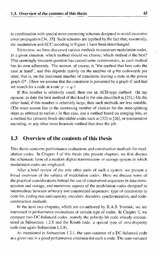
1.3. Overview of the contents of this thesis 45

in combination with special error-correcting schemes designed to avoid excessiveerror-propagation [34, 35]. Such schemes are typified by the fact that, essentially,the modulation and ECC encoding in Figure 1 have been interchanged.

Up to now, we have discussed various methods to construct modulation codes.In a given situation, which method should we choose; which method is the best?This seemingly innocent question has caused some controversies, as each methodhas its own adherends. The answer, of course, is "the method that best suits thecase at hand", and this depends mainly on the number of q-bit codewords perstate, that is, on the maximum number of transitions leaving a state in the powergraph C q . (Here we assume that the constraint is presented by a graph G and thatwe search for a code at a rate p ---+ q.)

If this number is relatively small, then use an ACH-type method. (In myopinion, to date the best method of this kind is the one described in [25].) On theother hand, if this number is relatively large, then such methods are less suitable.(The main reason lies in the increasing number of choices for the state-splittingsteps as referred to earlier.) In that case, use a method based on merging-bits, ora method for (almost) block-decodable codes such as [32] or [26], or enumerativeencoding, or any other more heuristic method that does the job.

1.3 Overview of the contents of this thesis

This thesis concerns performance evaluations and construction methods for mod­ulation codes. In Chapter I of this thesis (the present chapter), we first discussthe schematic form of a modern digital transmission- or storage system in whichmodulation codes are employed.

After a brief review of the role other parts of such a system, we present abroad overview of the subject of modulation codes. Here we discuss some ofthe practical considerations behind the use of constrained sequences in data trans­mission and storage, and numerous aspects of the modulation codes designed tointermediate between arbitrary and constrained sequences: type of constraints tocode for, coding rate and capacity, encoders, decoders, synchronization, and code­construction methods.

In the next two chapters, which are co-authored by K.A.S. Immink, we areinterested in performance evaluations of certain type of codes. In Chapter 2, wecompare two DC-balanced codes, namely the polarity-bit code already encoun­tered in Subsection 1.2.8 and the Knuth code, a special type of zero-disparitycode (see again Subsection 1.2.8).

As mentioned in Subsection 1.2.1, the sum-variance of a DC-balanced codeat a given rate is a good performance criterium for such a code. The sum-variance

46 1. Introduction

of a polarity-bit code is known to be a simple function of the codeword size,and hence of the rate, of the code. Things are not so simple for a Knuth code.My main contribution is an exact evaluation by combinatorial means of a goodapproximation to the sum-variance of a Knuth code. The result shows that thesum-variance of a Knuth code at a given rate is significantly larger than that of apolarity-bit code at the same rate, thus suggesting that polarity-bit codes have agreater spectral effectiveness than Knuth codes.

Magnetic recording systems commonly employ (d, k)-constrained sequencesto increase the efficiency of the recording channel. If such a constraint is used incombination with a synchronization method based on frames and unique headersas discussed in Subsection 1.2.7, then the requirement that the pattern used asheader is not allowed to occur in the bit-stream except at the beginning of a frameimposes an additional constraint on the sequences. In Chapter 3, we investigatethe loss of capacity entailed by imposing such an additional constraint. My maincontribution is a method based on generating functions to compute the capacity,the maximum possible coding rate, of this combined constraint, for any givenheader.

In the following three chapters, we introduce and investigate the class ofbounded-delay codes or BD codes, the class of sliding-block decodable codesfor constraints of finite type that can be encoded with a bounded encoding delayor, equivalently, by employing a bounded amount of look-ahead.

The ACH algorithm is one of the most important code construction methodsfor sliding-block decodable codes. As explained in Subsection 1.2.8, a drawbackof this method lies in the great freedom of choosing the state-splitting steps, es­pecially since the algorithm offers few clues how to strive for a code with a smalldecoding window.

The work in Chapter 4 addresses this problem. In this chapter, we first presenta precise definition and a thorough discussion of look-ahead encoders. Then wedevelop an algorithm especially designed to construct codes with a small decodingwindow. Our algorithm employs an approximate eigenvector and combines theweighted state-splitting from the ACH algorithm with ideas from the bounded­delay method of Franaszek. It is based on a new "local" construction method forBD codes where in each state of the weighted graph a certain partition problemhas to be solved. This partition problem can be interpreted as the problem ofdesigning a generic "local" look-ahead encoder in the state; this problem is easyto solve as long as the number of transitions leaving the state is not too large.

Once all these partition problems are successfully solved, it is easy to con­struct the desired BD code; here we can use the remaining freedom in the con­strnction to optimize the decoding window of the resulting code. This part of themethod is fully automatic and can be easily implemented in a computer program

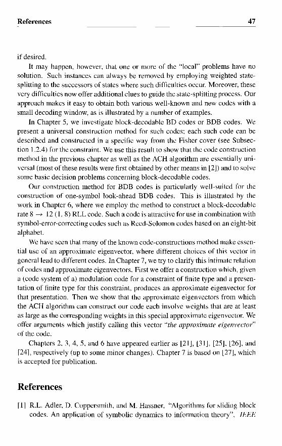
References 47

if desired.It may happen, however, that one or more of the "local" problems have no

solution. Such instances can always be removed by employing weighted state­s1"litting to the successors of states where such difficulties occur. Moreover, thesevery difficulties now offer additional clues to guide the state-splitting process. Ourapproach makes it easy to obtain both various well-known and new codes with asmall decoding window, as is illustrated by a number of examples.

In Chapter 5, we investigate block-decodable BD codes or BDB codes. Wepresent a universal construction method for such codes; each such code can bedescribed and constructed in a specific way from the Fisher cover (see Subsec­tion 1.2.4) for the constraint. We use this result to show that the code constructionmethod in the previous chapter as well as the ACH algorithm are essentially uni­versal (most of these results were first obtained by other means in [2]) and to solvesome basic decision problems concerning block-decodable codes.

Our construction method for BDB codes is particularly well-suited for theconstruction of one-symbol look-ahead BDB codes. This is illustrated by thework in Chapter 6, where we employ the method to construct a block-decodablerate 8 ----+ 12 (l, 8) RLL code. Such a code is attractive for use in combination withsymbol-error-correcting codes such as Reed-Solomon codes based on an eight-bitalphabet.

We have seen that many of the known code-constructions method make essen­tial use of an approximate eigenvector, where different choices of this vector ingeneral lead to different codes. In Chapter 7, we try to clarify this intimate relationof codes and approximate eigenvectors. First we offer a construction which, givena (code system of a) modulation code for a constraint of finite type and a presen­tation of finite type for this constraint, produces an approximate eigenvector forthat presentation. Then we show that the approximate eigenvectors from whichthe ACH algorithm can construct our code each involve weights that are at leastas large as the corresponding weights in this special approximate eigenvector. Weoffer arguments which justify calling this vector "the approximate eigenvector"of the code.

Chapters 2,3,4,5, and 6 have appeared earlier as [21], [31], [25], [26], and[24], respectively (up to some minor changes). Chapter 7 is based on [27], whichis accepted for publication.

References

[1] R.L. Adler, D. Coppersmith, and M. Hassner, "Algorithms for sliding blockcodes. An application of symbolic dynamics to information theory", IEEE

48 References

Trans. Inform. Theory. vol. IT-29, no. 1, pp. 5-22, Jan. 1983.

[2] J. Ashley and B.H. Marcus, "Canonical encoders for sliding block decoders".Siam J. Disc. Math., vol. 8, no. 4, pp. 555-605, Nov. 1995.

[3] M.-P. Beal, Codage symbolique, Paris: Masson, 1993.

[4] G.EM. Beenker and K.AS. Immink, "A generalized method for encoding anddecoding run-length-limited binary sequences", IEEE Trans. Inform. Theory,vol. IT-29, no. 5, pp. 751-754, Sept. 1983.

[5] S. Benedetto and G. Montorsi "Unveiling turbo codes: some results on par­allel concatenated coding schemes", IEEE Trans. Inform. Theory, vol. 42,no. 2, pp. 409-429, June 1996.

[6] C. Berrou, A Glavieux, and P Thitimajshima, "Near Shannon limit error­correcting coding and decoding: turbo codes", Proc. ICC '93, pp. 1064-1070.

[7] AR. Calderbank (Ed.), Different aspects of coding theory, Providence, RI:AMS, 1995.

[8] T.M. Cover. "Enumerative source coding", IEEE Trans. Inform. Theory,vol. IT-19, pp. 73-77, Jan. 1973.

[9] T.M. Cover and J.A Thomas, Elements of information theory, New York:Wiley, 1991.

[10] J.S. Eggenberger and P Hodges, "Sequential encoding and decoding ofvariable word length, fixed rate data codes", U.S. Patent 4,115,768. 1978.

[11] M. Feteke, Math. Zeitschr., vol. 17, pp. 233,1923.

[12] G.D. Forney, Jr., "Generalized minimum distance decoding", IEEE Trans.Ir~form. Theory. vol. 12, pp. 125-131, 1966.

[13] P.A Franaszek, "Sequence-state coding for digital transmission", Bell Syst.Tech. J., vol. 47, pp. 143-157, Jan. 1968.

[14] PA Franaszek, "On future-dependent block coding for input-restrictedchannels", IBM J. Res. Develop., vol. 23, pp. 75-81, Jan. 1979.

[15] P.A Franaszek, "Synchronous bounded delay coding for input restrictedchannels", IBM J. Res. Develop., vol. 24, pp. 43-48, Jan. 1980.

[16] PA Franaszek, "A general method for channel coding", IBM J. Res. De­velop., vol. 24, pp. 638-641, Sept. 1980.

References 49

[17] P.A. Franaszek, "Construction of bounded delay codes for discrete noiselesschannels". IBM J. Res. Develop., vol. 26, pp. 506-514. July 1982.

[18] P.A. Franaszek, "Coding for constrained channels: A comparison of twoapproaches", IBM J. Res. Develop., vol. 33. pp. 602-608, Nov. 1989.

[19] J. Gu and T. Fuja, "A new approach to constructing optimal block codes forrunlength-limited channels", IEEE Trans. Inform. Theory, vol. ITAO, no. 3,pp. 774-785,1994.

[20] J. Gu and T. Fuja, "A note on look-ahead in the encoders of block-decodable(d, k) codes", preprint.

[21] H.D.L. Hollmann and K.A.S. Immink, "Performance of efficient balancedcodes", IEEE Trans. Inform. Theory, vol. 37, no. 3, pp. 913-918, May 1991.

[22] H.D.L. Hollmann, "The general solution of write equalization for RLL (d, k)

codes", IEEE Trans. Inform. Theory, vol. 37, no. 3, Part II, pp. 856-862, May1991, special issue on "Coding for storage devices".

[23] H.D.L. Hollmann, "Bounded-delay encodable codes for constrained systemsfrom state combination and state splitting", Benelux Symp. Inform. Theory,Veldhoven, May 1993.

[24] H.D.L. Hollmann, "A block-decodable (d, k) = (1,8) run-length-limitedrate 8/12 code", IEEE Trans. Inform. Theory, vol. 40, no. 4, pp. 1292-1296,July 1994.

[25] H.D.L. Hollmann, "On the construction of bounded-delay encodable codesfor constrained systems", IEEE Trans. Inform. Theory, vol. 41, no. 5, pp.1354-1378, Sept. 1995.

[26] H.D.L. Hollmann, "Bounded-delay encodable, block-decodable codes forconstrained systems", IEEE Trans. Inform. Theory, vol. 42, no. 6. Nov. 1996,special issue on "Codes and complexity".

[27] H.D.L. Hollmann, "On an approximate eigenvector associated with a mod­ulation code", accepted for publication in IEEE Trans. Inform. Theory.

[28] J.E. Hopcroft and J.D. Ullmann, Formal languages and their relation toautomata, Reading, MA: Addison-Wesley, 1969.

[29] J.E. Hopcroft and J.D. Ullmann, Introduction to automata theory, languages,and computation, Reading, MA: Addison-Wesley, 1979.

so References

[30] KA.S.lmmink, Coding techniquesfordigital recorders, Englewood Cliffs,NY: Prentice-Hall, 1991.

[31] KA.S. Immink and H.D.L. Hollmann, "Prefix-synchronized run-length­limited sequences", IEEE J. Sei. Areas Commun., vol. 10, no. 1, pp. 214-222,Jan. 1992.

[32] KA.S. Immink, "Block-decodable run-length-limited codes via look-aheadtechnique", Philips J. Res., vol. 46, no. 6, pp. 293-310, 1992.

[33] KA.S. Immink, "Constructions of almost block-decodable runlength­limited codes", IEEE Trans. Inform. Theory, vol. 41, no. 1, pp. 284-287, Jan.1995.

[34] KA.S. Immink, "A practical methos for approaching the channel capacityof constrained channels" submitted to IEEE Trans. Inform. Theory.

[35] KA.S. Immink, "EFM coding: squeezing the last bits" submitted to IEEETrans. Consumer Electr..

[36] G. Jacoby and R. Kost, "Binary two-thirds rate code with full word look­ahead", IEEE Trans. Magnet., vol. MAG-20, no. 5, pp. 709-714, Sept. 1984.

[37] A. Lempel and M. Cohn, "Lookahead coding for input-restricted channels",IEEE Trans. Inform. Theory, vol. IT-28, pp. 933-937, Nov. 1982.

[38] D. Lind and B. Marcus, An introduction to symbolic dynamics and coding,Cambridge, MA: Cambridge University Press, 1995.

[39] J.H. van Lint, Coding theory, New York: Springer, 1971.

[40] F.J. MacWilliams and N.J.A. Sloane, The theory of error-correcting codes,Amsterdam: Elsevier, 1977.

[41] B.H. Marcus and R. Roth, "Bounds on the number of states in encodergraphs for input-constrained channels", IEEE Trans. Inform. Theory, vol. IT­37, no. 3, pp. 742-758, May 1991.

[42] B.H Marcus, P.H. Siegel, and J.K Wolf, "Finite-state modulation codes fordata storage", IEEE J. Sei. Areas Commun., vol. 10, no. 1, pp. 5-37, Jan.1992.

[43] H. Minc, Nonnegative matrices, New York: Wiley, 1988.

References 51

[44] H. Nyquist, "Certain factors affecting telegraph speed", Bell Syst. Tech. J.,vol. 3, p. 324, 1924.

[45] L. Patrovics and K.A.S. Immink, "Encoding of dklr-sequences using oneweight set", IEEE Trans. Inform. Theory, vol. 42, no. 5, pp. 1553-1554, Sept.1996.

[46] G. P61ya and G. Szego, Aufgaben und Lehrsiitze aus der Analysis, Berlin:Springer, 1970.

[47] E. Seneta, Non-negative matrices and Markov chains (Second ed.), NewYork: Springer, 1981.

[48] C. Shannon, "A mathematical theory of communication", Bell Syst. Tech.J., vol. 27, pp. 379-423,623-656, October 1948.

[49] C. Shannon, "Communication in the presence of noise", Proc. IRE, vol. 37,pp. 10-21, 1949.

[50] R.C. Schneider, "Write equalization in high-density magnetic recording",IBM J. Res. Develop., vol. 29, no 6, Nov. 1985.

[51] R.C. Schneider, "Write equalization for generalized (d, k) codes", IEEETrans. Magnet., vol. MAG-24, no. 6, pp. 2533-2535, Nov. 1988.

[52] L.M.G. To1huizen, "Cooperating error-correcting codes and their decoding",Doctoral thesis, Eindhoven Un. Techn., Eindhoven, June 1996.

[53] J.H. Weber and K.A. Abdel-Ghaffar, "Cascading Runlength-Limited Se­quences", IEEE Trans. Inform. Theory, vol. IT-39, no. 6, pp. 1976-1984, Nov.1993.

[54] B. Weiss, "Subshifts of finite type and sofie systems", Monats. Math.,vol. 77,pp.462-474, 1973.

[55] H.W. Wong-Lam, H.D.L. Hollmann, "A general solution of write equaliza­tion for digital magnetic recording", IEEE Trans. Magnet., vol. MAG-27,no. 5, pp. 4377-4381, Sept. 1991.

[56] A.D. Wyner, "Capabilities of bounded discrepancy decoding", Bell Syst.Tech. J., vol. 54, pp. 1061-1122, 1965.

Chapter 2

Performance of EfficientBalanced Codes

Abstract - Recently, Knuth presented coding schemes in which each codewordcontains equally many "zeros" and "ones". The construction has the virtue that thecodes can be efficiently encoded and decoded. In this correspondence, we addressthe problem of appraising the spectral performance of codes based on Knuth's algo­rithm.

Index Terms - dc-balanced codes, Knuth codes, sum variance.

2.1 Introduction

Binary sequences with spectral nulls at zero frequency have found widespread ap­plication in optical and magnetic recording systems. These dc-balanced codes,as they are often called, have a long history and their application is certainlynot confined to recording practice. Since the early days of digital communica­tion over cable, dc-balanced codes have been employed to counter the effects oflow-frequency cut-off due to coupling components, isolating transformers, etc.In optical recording, as explained in [3], dc-balanced codes are employed to cir­cumvent or reduce interaction between the data written on the disc and the servosystems that follow the track. A present-day application of dc-free codes [4] is thedigital audio tape recorder which uses an 8b1Db code to circumvent the effects ofcrosstalk from adjacent tracks, and to minimize over-write noise.

© 1991, IEEE. Reprinted, with permission, from IEEE Transactions on Information Theoryvol. 37, no. 3, pp. 913-918, May 1991.

Co-authored by K.A. Schouhamer Immink.This work was presented in part at the IEEE International Workshop on Information Theory,

Veldhoven, The Netherlands. 1990.

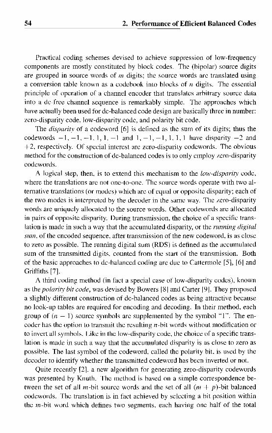
54 2. Performance of Efficient Balanced Codes

Practical coding schemes devised to achieve suppression of low-frequencycomponents are mostly constituted by block codes. The (bipolar) source digitsare grouped in source words of m digits; the source words are translated usinga conversion table known as a codebook into blocks of n digits. The essentialprinciple of operation of a channel encoder that translates arbitrary source datainto a dc-free channel sequence is remarkably simple. The approaches whichhave actually been used for dc-balanced code design are basically three in number:zero-disparity code, low-disparity code, and polarity bit code.

The disparity of a codeword [6] is defined as the sum of its digits; thus thecodewords -1, -1, -1, 1, 1, -1 and 1, -1, -1, 1, 1, 1 have disparity -2 and+2, respectively. Of special interest are zero-disparity codewords. The obviousmethod for the construction of dc-balanced codes is to only employ zero-disparitycodewords.

A logical step, then, is to extend this mechanism to the low-disparity code,where the translations are not one-to-one. The source words operate with two al­ternative translations (or modes) which are of equal or opposite disparity; each ofthe two modes is interpreted by the decoder in the same way. The zero-disparitywords are uniquely allocated to the source words. Other codewords are allocatedin pairs of opposite disparity. During transmission, the choice of a specific trans­lation is made in such a way that the accumulated disparity, or the running digitalsum, of the encoded sequence, after transmission of the new codeword, is as closeto zero as possible. The running digital sum (RDS) is defined as the accumulatedsum of the transmitted digits, counted from the start of the transmission. Bothof the basic approaches to dc-balanced coding are due to Cattermo1e [5], [6] andGriffiths [7].

A third coding method (in fact a special case of low-disparity codes), knownas the polarity bit code, was devised by Bowers [8] and Carter [9]. They proposeda slightly different construction of dc-balanced codes as being attractive becauseno look-up tables are required for encoding and decoding. In their method, eachgroup of (n - 1) source symbols are supplemented by the symbol "1". The en­coder has the option to transmit the resulting n-bit words without modification orto invert all symbols. Like in the low-disparity code, the choice of a specific trans­lation is made in such a way that the accumulated disparity is as close to zero aspossible. The last symbol of the codeword, called the polarity bit, is used by thedecoder to identify whether the transmitted codeword has been inverted or not.

Quite recently [2], a new algorithm for generating zero-disparity codewordswas presented by Knuth. The method is based on a simple correspondence be­tween the set of all m-bit source words and the set of all (rn + p )-bit balancedcodewords. The translation is in fact achieved by selecting a bit position withinthe m-bit word which defines two segments, each having one half of the total

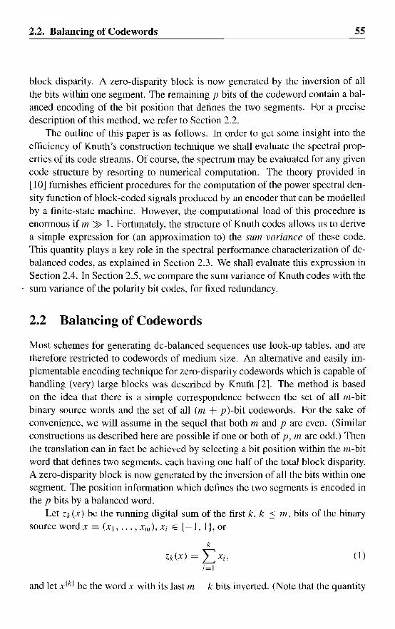
2.2. Balancing of Codewords 55

(1)

block disparity. A zero-disparity block is now generated by the inversion of allthe bits within one segment. The remaining p bits of the codeword contain a bal­anced encoding of the bit position that defines the two segments. For a precisedescription of this method, we refer to Section 2.2.

The outline of this paper is as follows. In order to get some insight into theefficiency of Knuth's construction technique we shall evaluate the spectral prop­erties of its code streams. Of course, the spectrum may be evaluated for any givencode structure by resorting to numerical computation. The theory provided in[10] furnishes efficient procedures for the computation of the power spectral den­sity function of block-coded signals produced by an encoder that can be modelledby a finite-state machine. However, the computational load of this procedure isenormous if m » 1. Fortunately, the structure of Knuth codes allows us to derivea simple expression for (an approximation to) the sum variance of these code.This quantity plays a key role in the spectral performance characterization of dc­balanced codes, as explained in Section 2.3. We shall evaluate this expression inSection 2.4. In Section 2.5, we compare the sum variance of Knuth codes with thesum variance of the polarity bit codes, for fixed redundancy.

2.2 Balancing of Codewords

Most schemes for generating dc-balanced sequences use look-up tables, and aretherefore restricted to codewords of medium size. An alternative and easily im­plementable encoding technique for zero-disparity codewords which is capable ofhandling (very) large blocks was described by Knuth [2]. The method is basedon the idea that there is a simple correspondence between the set of all m-bitbinary source words and the set of all (m + p )-bit codewords. For the sake ofconvenience, we will assume in the sequel that both m and p are even. (Similarconstructions as described here are possible if one or both of p, m are odd.) Thenthe translation can in fact be achieved by selecting a bit position within the m-bitword that defines two segments, each having one half of the total block disparity.A zero-disparity block is now generated by the inversion of all the bits within onesegment. The position information which defines the two segments is encoded inthe p bits by a balanced word.

Let Zk (x) be the running digital sum of the first k, k :::: m, bits of the binarysource word x = (Xl, ... ,XIII)' X; E {-I, I}, or

k

Zk(X) = LX;,;=1

and let x[k] be the word X with its last m - k bits inverted. (Note that the quantity

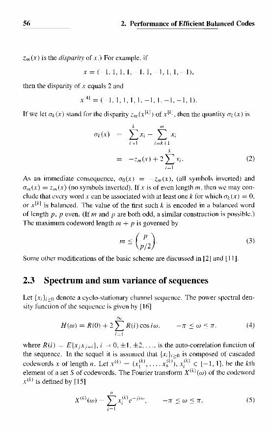
56 2. Performance of Efficient Balanced Codes

2m (x) is the disparity of .er.) For example, if

X = (-1, 1, 1, 1, -1, 1, -1,1,1, -1),

then the disparity of X equals 2 and

x[4] = (-1. 1, 1, 1, 1, -1, 1, -1. -1, I).

If we let (Tk(X) stand for the disparity Z/Il (x[k]) of x[k], then the quantity (Tk (x) is

k m

(Tk(X) = LXi - L Xii=] i=k+l

k

-Zm(X) + 2 LXi.i=]

(2)

As an immediate consequence, (TO(X) -Zm(X), (all symbols inverted) and(Tm (x) = Zm (x) (no symbols inverted). If x is of even length 111, then we may con­clude that every word x can be associated with at least one k for which (Tk (x) = 0,or x lk] is balanced. The value of the first such k is encoded in a balanced wordof length p, p even. (If 111 and p are both odd, a similar construction is possible.)The maximum codeword length 111 + P is governed by

(3)

Some other modifications of the basic scheme are discussed in [2] and [11].

2.3 Spectrum and sum variance of sequences

Let {Xi L::::o denote a cyclo-stationary channel sequence. The power spectral den­sity function of the sequence is given by [16]

00

H(w) = R(O) + 2L R(i) cos iw.i=l

-Jr .:::: w .:::: Jr, (4)

where R(i) = E{XjXj+i}, i = 0, ±1, ±2, ... , is the auto-correlation function ofthe sequence. In the sequel it is assumed that {Xdi>O is composed of cascaded

d d , f I h L (k) (k) (k) - Jk) {II} b h k hco ewor s x 0 engt n. et x = Xl , ... , X n ), Xi E -, , e t e telement of a set S of codewords. The Fourier transform X(k) (w) of the codewordx (k) is defined by [15]

n

X(k)(w) = Lx?)e- iiw ,

i=l

-Jr .:::: w .:::: Jr, (5)

2.3. Spectrum and sum variance of sequences 57

where j = R. For all i. 1 ::: i ::: 11. let the number of codewords x(k) E S withx?) = 1 be equal to the number of codewords with x?) = -1 (i.e., the sum ofall codewords in S is the all-zero vector). If, in addition, codewords are randomlychosen from S to form an infinite sequence, then it is rather straightforward toshow, following [16] and [17], that the power spectral density function H (w) ofthe concatenated sequence is

(6)

Note that, due to our assumptions, lSI has to be even. We will assume that thecodewords are equiprobable.

From now on, we assume that the set of codewords S forms a dc-balancedcode, in other words, the disparity of all the members of S is zero. The widthof the spectral notch is a relevant quantity since it specifies the frequency regionof suppressed components around the spectral null. Let H (w) denote the powerspectral density function of the sequences formed by cascading the codewords.Then the width of the spectral notch is defined by a quantity called the cut-offfrequency. The cut-off frequency. denoted by (Vo. is defined by [13], [14]

1H(wo) = 2' (7)

Another quantity used in the performance evaluation of codes with a null at thezero frequency is the running digital sum [12]. The running digital sum Zj isdefined by

(8)

Specifically, the variance of the running digital sum, in short sum variance, playsa key role in the spectral performance characterization of dc-balanced codes. Thesum variance of the encoded sequence is defined as

2 2S = E{Z,}, (9)

where E {.} denotes the expectation operator. It was found by Justesen [13] thatfor dc-free sequences the product of cut-off frequency Wo and the sum variance ofthe sequence is approximately 1/2, or

(10)

It has been found that this relationship between the sum variance and the actualcut-off frequency is accurate within a few percent [12]. On the other hand, the

58 2. Performance of Efficient Balanced Codes

sum variance is relevant in its own right as it gives the variance of the intersymbolinterference when the channel is ac-coupled.

As in the case of H (w), it can be shown that, under similar conditions, thesum variance s2 of the concatenated sequence is [I2J

(11)

where Zj(x) := 'L,{=I Xi and lSI denotes the cardinality of S. (Observe thatlSI = 211l

.)

In principle, the above equations can be invoked to compute the spectrum andsum variance of sequences generated by Knuth's method. In that case, S con­sists of the collection of (m + p )-bit codewords obtained from the set of all m-bitsource words as described in Section 2.2. Naturally, the above operation of enu­merating all codewords is, for large codeword sets, a considerable computationalload. (Recall that ISI = 2m .) The computational load can be alleviated by makingsome approximations. Ignoring the contribution from the p-bit vector (note thatKnuth's algorithm is especially designed for large codewords, i.e., p « m), thesum variance can be approximated as

(l2)

This approximation is justified mathematically by the facts that

1) zlIl(y)=O,foryES,and2) (lIn) 'L,~=1[Zj(u)J2 = O(p3Im) = oem), m -+ 00, for a balanced p-bitword u.

In the next section we shall evaluate the right-hand side in (12) exactly.

2.4 A counting problenl

In this section we shall provide an exact evaluation of the right-hand side of theapproximation for s2 in (12). We first introduce some useful notation. Throughoutthis section, 111 denotes an even, positive integer. The collection of all binary wordsx = (Xl •...• Xm), xi E {-I, I}, will be denoted by Rm . For x E Rm , we definez(x) = Vo(x), ... , Zm(x)) by

k

Zk(X) := LXi,

i=J

(13)

2.4. A counting problem

k = 0, ... , m. (Note that zo(x) = °by convention. Note also that Zk(X)k mod 2.) Put

Sm := {z(x) I x E Rm}.

For each integer k, -m :s k :s m, we let i

Rm(k) := {x E Rm I Zm(x) = k}

and

Sm(k) := {z E Sm I Zm = k}.

59

Let x E Rm. The quantity Zk (x) - (1 j2)zm (x) starts at -(1 j2)zm (x) for k = 0,ends at (1 j2)zm (x) for k = m, and increases by ± 1 if k increases by 1. Since m iseven, we conclude that there exists a smallest integer l = l (x), °:s l (x) :s m - 1,for which ZI(X) = (1j2)zm(x). Define xby

(14)

(15)

with l = lex) as defined above. Observe that in Knuth's method a word x isencoded as a word with initial part x. Observe also that x E Rm (0), in otherwords, x is balanced.

Next, let Z E Sm, with Z = z(x), say. (Note that x is uniquely determined byz.) By abuse of notation, we set l(z) := lex), and we letzbe defined byz:= z(X).In other words,

~ {Zk, ifO:sk:sl(z);Zk:= Zm - Zk, if l(z) :s k :s m.

Note thatZ E Sm (0) by definition. Moreover, observe thatZcan be obtained fromZ by a reflexion of the part (Zl, ... , Zm) of Z with respect to the line y = (1 j2)zm.(See Figure 1.)

With the above definitions, the approximation (12) can now be expressed as

where the quantity Jc(m) is defined as

m

Jc(m) := L LzJ.ZESm j=l

Our aim is to prove the following result.

(16)

(17)

60 2. Performance of Efficient Balanced Codes

Zm

m

Z

kl(z)o

I 12Zm f------------,"",..-.----¥-------;-~---+-Y = 2Zm

I "0.I '0.I '0.I "0.

I •••••••, .,,

Figure 1: The relation between Z andz.

Theorem 1: A(m) = m(3m + 2)2m-

4 .

The proof of the above theorem will depend on a number of lemmas and usesinduction on m. (It is easily verified that Theorem (1) indeed holds for smallvalues of m.) In the course of our computations, we will frequently make use ofthe following two results. Let 17ij and Pij, 1 ::: i, j ::: m, be defined by

17ij := 2-m L XiXj,

XERm

Pij := ( m )-1 L XiXj.

mj2 xERm(O)

(18)

Lemma 2: We have

17ij = { I,0,

if i = j;otherwise.

(19)

Proof Evident.

Lemma 3: We have

o

{I,

Pij = -1j(m - 1),if i = j;otherwise.

(20)

Proof By symmetry, Pij only depends on whether or not i = j holds. More­over, from the definition of Rm (0) we find that L:J=l Pij = O. Since it is immedi­ate that Pii = 1, the result now follows. 0

Lemmas 2 and 3 indicate that it is easy to compute a sum over Sm or Sm (0) ofpolynomial functions of the Zj only (i.e., not involving the Zj), simply by writingout the sum in terms of the x j .

Our next result simplifies the expression (17) for A(m).

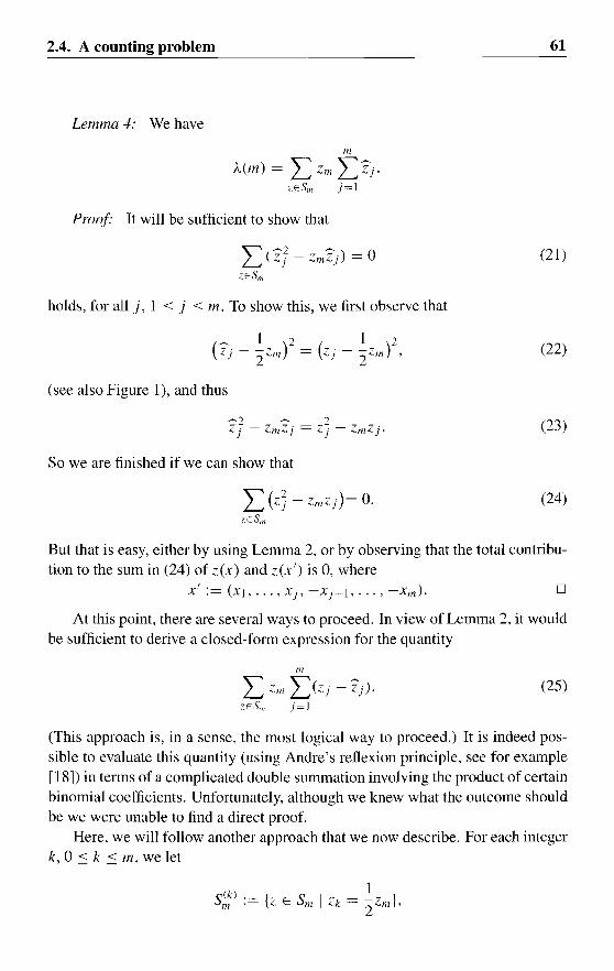
2.4. A counting problem

Lemma 4: We have

11/

A(m) = L Zm L0'ZESm j=l

Proof It will be sufficient to show that

L CZ7 - ZmZj) = 0ZESm

holds, for all j, 1 ::s j ::s m. To show this, we first observe that

(see also Figure 1), and thus

~2 ~ 2Zj - ZmZj = Zj - ZmZj.

So we are finished if we can show that

L (Z] - ZmZj)= O.ZESm

61

(21)

(22)

(23)

(24)

But that is easy, either by using Lemma 2, or by observing that the total contribu­tion to the sum in (24) of Z(x) and Z (x') is 0, where

x' := (Xl, ... , Xj, -Xj+l, ... , -Xm)' D

At this point, there are several ways to proceed. In view of Lemma 2, it wouldbe sufficient to derive a closed-form expression for the quantity

m

L ZII/ L(Zj - Zj).ZESm j=J

(25)

(This approach is, in a sense, the most logical way to proceed.) It is indeed pos­sible to evaluate this quantity (using Andre's reflexion principle, see for example[18]) in terms of a complicated double summation involving the product of certainbinomial coefficients. Unfortunately, although we knew what the outcome shouldbe we were unable to find a direct proof.

Here. we will follow another approach that we now describe. For each integerk,O ::s k ::s m, we let

62 2. Performance of Efficient Balanced Codes

d f S Ck) d fi -Ck) - ry(k) Ck)) ban or Z Em, we e ne ~ - (."0 ."', Zm Y

(kJ '_ { Zj,Z· ,-J Zm - Zj,

ifO::;}::;k;if k < } ::; m,

(26)

Observe that Z(k) E SII/ (0) for all Z E S~k), and Z(kJ = Z if k = I (z), So we maywrite

m

A(m) L 2m LZjZESm j=]

(To see this, note that each Z E Sm contributes Zm LJ=l <k) to the first summation

in (27) for each k such that Z E S~k), By definition of I (::J, the smallest such kequals I(z) and gives a contribution equal to Zm LJ=l Zj, while the contributionsfor all k > I occur also in the second summation in (27).) We will evaluate thetwo parts of (27) for A(m) separately.

Lemma 5:

2 L (f>jrIIESII/CO) J=l

I 1 . ( m )-m-(m + I) .6 m/2

Proof For fixed k, the map z f-+ ZCk) defines a one-to-one cOlTespondencebetween S:!:J and Sm (0). Indeed, note that the inverse of this map is the map

U f-+ (Ul, .... Uk, 2Uk - Uk+[ .... , 2Uk - Um-l, 2Uk).

Since Zm = 2Zk = 2zkk) for all 2 E S~~) by definition of S:!:), the first equationfollows. To evaluate the second sum, write

(

m )2L LUj

UESm CO) j=l(28)

and use Lemma 3, together with the two well-known series

L~=o k = (1/2)m(m + 1) and L~=o k2 = (l/6)m(m + 1)(2m + I).

2.4. A counting problem

We leave all further details to the reader.

Lemma 6:m m

L L L ZmLZ)k)k=O O::ol<k ZESf;~) j=1

l(z)=l

m-2 ( ) { }~ n~2 )..(111 - n) + ~n(m - n)2111

-11

•

11=0 mod 2

63

o

(31)

Proof Fix k and l, with 0 :s l < k, and put n := k -l. Let Z E S:!:), withl(z) = l. (Observe that this is possible only if n is even.) With each such z, weassociate a pair of sequences a(z) and b(z), defined as follows.

aj(Z):= {Zj. if 0 :s j :s l; (29)Zj+n, if l < j :s m - n,

Ibj(z) := Zj+l - 2Zm, O:s j :s n. (30)

Observe that b(z) represents the part of Z between indices land k, and sinceZk = Zl = (l/2)zm by our assumptions on Z, it follows that b(z) E Sn (0). Observealso that a(z) can be obtained by removing from Z the part of Z between indicesl + ] and k, and thus a(z) E Sm-n, l(a(z)) = l(z) = land am-n(Z) = Zm. (Seeagain Figure 1.) From these observations, and from the definition of Z(k), we findthat

111 { m-n n I }Zm f;Z)k) = am-n(Z) f; a7(Z) + t;[biCZ) + 2 am - lI (z)] .

Conversely, each pair a and b for which a E Sm-n, lea) = land b E Sn(O)determines, through (29) and (30), a unique Z E S~k) with l (z) = l such thata(z) = a and b(z) = b. By this observation, we find from (3]) that

{m-n It I }

L Lam-II L fij + L bi + -nam- naESm _ n bESn(O) j=1 i=1 2l(a)=l

(n~2) L {am-l1I:fij+~na;_II}' (32)aESm - n 1=1l(a)=l

where the last equation follows from the trivial observation that

(33)

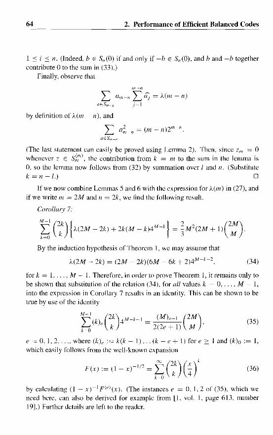
64 2. Performance of Efficient Balanced Codes

1 ::::: i ::::: n. (Indeed, b E Sn (0) if and only if -b E Sn (0), and band -b togethercontribute °to the sum in (33).)

Finally, observe that

m--n

L am - n La; = A(1ll - n)aESrn - n j=1

by definition of A(m - n), and

L a;1~n = (m - n)2m-

n.

aESrn - n

(The last statement can easily be proved using Lemma 2). Then, since Zm = °whenever Z E S~m), the contribution from k = m to the sum in the lemma is0, so the lemma now follows from (32) by summation over land 11. (Substitutek = n -l.) 0

If we now combine Lemmas 5 and 6 with the expression for A(m) in (27), andif we write m = 2M and n = 2k, we find the following result.

Corollary 7:

M-l (2k) { } 2 (2M)6 k A(2M - 2k) + 2k(M - k)4M-

k = }M2(2M + 1) M .

By the induction hypothesis of Theorem 1, we may assume that

A(2M - 2k) = (2M - 2k)(6M - 6k + 2)4M - k - 2 , (34)

(35)

(36)

for k = 1, ... , M - 1. Therefore, in order to prove Theorem 1, it remains only tobe shown that substitution of the relation (34), for all values k = 0, ... , M - 1,into the expression in Corollary 7 results in an identity. This can be shown to betrue by use of the identity

M-l (2k) (M) (2M)L (k)e 4M - k- 1 = e+l ,k=O k 2(2e + 1) M

e = 0, 1,2, ... , where (k)e := k(k - 1) ... (k - e + 1) for e :::: I and (k)o := 1,which easily follows from the well-known expansion

F(x) := (l _ x)-1/2 = f: (2k) (~)kk=O k 4

by calculating (l - x·)-I F(e)(x). (The instances e = 0,1,2 of (35), which weneed here, can also be derived for example from [1, vol. 1, page 613, number19].) Further details are left to the reader.

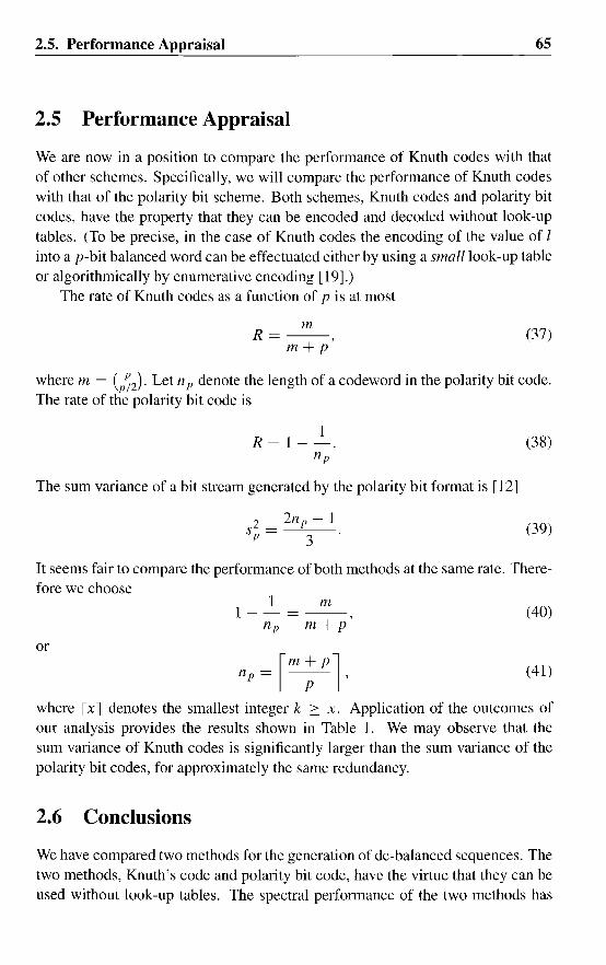
2.5. Performance Appraisal

2.5 Performance Appraisal

65

We are now in a position to compare the performance of Knuth codes with thatof other schemes. Specifically, we will compare the performance of Knuth codeswith that of the polarity bit scheme. Both schemes, Knuth codes and polarity bitcodes, have the property that they can be encoded and decoded without look-uptables. (To be precise, in the case of Knuth codes the encoding of the value of Iinto a p-bit balanced word can be effectuated either by using a small look-up tableor algorithmically by enumerative encoding [19].)

The rate of Knuth codes as a function of p is at most

mR=--,

m+p(37)

where m = (pj2)' Let npdenote the length of a codeword in the polarity bit code.The rate of the polarity bit code is

1R = 1--.

n p

The sum variance of a bit stream generated by the polarity bit format is [12]

2 2n p - 1s = -'------

p 3

(38)

(39)

It seems fair to compare the performance of both methods at the same rate. There­fore we choose

or

1 m1--=--,

n p m+ p(40)

(41 )_1 m + pln p - ,p

where IX1 denotes the smallest integer k :::: x. Application of the outcomes ofour analysis provides the results shown in Table 1. We may observe that thesum variance of Knuth codes is significantly larger than the sum variance of thepolarity bit codes, for approximately the same redundancy.

2.6 Conclusions

We have compared two methods for the generation of dc-balanced sequences. Thetwo methods, Knuth's code and polarity bit code, have the virtue that they can beused without look-up tables. The spectral performance of the two methods has

66 References

S2p

36.33

17.6751.67

164.33537

1801.67

n p

5102778

247806

2703

')s­

K

3.87513.25047.375

173.375643.625

2413.2509116.375

Table 1: Rate and sum variance of Knuth codes and polarity bit codes versuscode~vord length n = m + p.

p m 1- R

6 20 0.23088 70 0.1026

10 252 0.038212 924 0.012814 3432 0.004116 12870 0.001218 48620 0.0004

been evaluated with a parameter called the sum variance. Under the premise thatthe sum variance can serve as a quantity to judge the width of the spectral notch,we conclude that codes based on Knuth's algorithm offer less spectral suppressionthan polarity bit codes with the same redundancy.

Acknowledgement

It is a great pleasure to thank our colleagues J.H. van Lint, Sr. and L. Tolhuizenfor some fruitful discussions.

References

[1] AP. Prudnikov, Yu.A Brychkov, and 0.1. Marichev, Integrals and series,Gordon and Breach Science Publishers.

[2] D.E. Knuth, "Efficient Balanced Codes", IEEE Trans. Inform. Theory, vol.IT-32, pp. 51-53, Jan. 1986. See also PS. Henry, "Zero disparity codingsystem", US Patent 4,309,694, Jan. 1982.

[3] J.P.J. Heemskerk and KAS. Immink, "Compact Disc: System Aspects andModulation", Philips J. Res., vol. 40, No.6, pp. 157-164, 1982.

[4] S. Fukuda, Y. Kojima, Y. Shimpuku, and K Odaka, "8110 Modulation Codesfor Digital Magnetic Recording", IEEE Trans. Magnet., vol. MAG-22, pp.1194-1197, Sept. 1986.

[5] KW. Cattermole, "Principles of Digital Line Coding", Int. J. Electron., vol.55, pp. 3-33, July 1983.

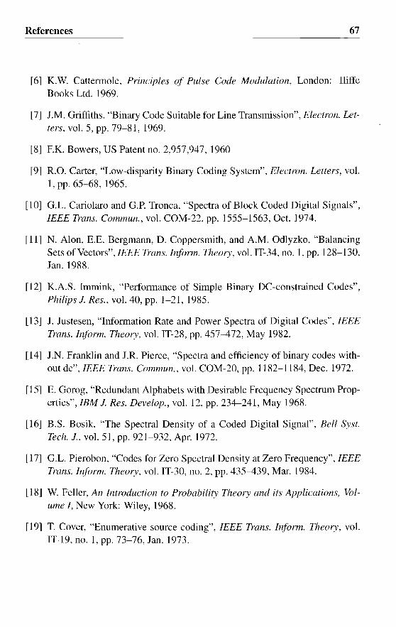
References 67

[6] K.W. Cattennole, Principles of Pulse Code Modulation, London: IliffeBooks Ltd, 1969.

[7] J.M. Griffiths, "Binary Code Suitable for Line Transmission", Electron. Let­ters, vol. 5, pp. 79-81, 1969.

[8] F.K. Bowers, US Patent no. 2,957,947, 1960

[9] R.O. Carter, "Low-disparity Binary Coding System", Electron. Letters, vol.1, pp. 65-68, 1965.

[10] G.L. Cariolaro and G.P. Tronca, "Spectra of Block Coded Digital Signals",IEEE Trans. Commun., vol. COM-22, pp. 1555-1563, Oct. 1974.

[11] N. Alon, E.E. Bergmann, D. Coppersmith, and A.M. Odlyzko, "BalancingSets of Vectors", IEEE Trans. Inform. Theory, vol. IT-34, no. I, pp. 128-130,Jan. 1988.

[12] K.A.S. Immink, "Performance of Simple Binary DC-constrained Codes",Philips J. Res., vol. 40, pp. 1-21, 1985.

[13] J. Justesen, "Information Rate and Power Spectra of Digital Codes", IEEETrans. Inform. Theory, vol. IT-28, pp. 457-472, May 1982.

[14] J.N. Franklin and J.R. Pierce, "Spectra and efficiency of binary codes with­out dc", IEEE Trans. Commun., vol. COM-20, pp. 1182-1184, Dec. 1972.

[15] E. Gorog, "Redundant Alphabets with Desirable Frequency Spectrum Prop­erties", IBM J. Res. Develop., vol. 12, pp. 234-241, May 1968.

[16] B.S. Bosik, "The Spectral Density of a Coded Digital Signal", Bell S.vst.Tech. J., vol. 51, pp. 921-932, Apr. 1972.

[17] G.L. Pierobon, "Codes for Zero Spectral Density at Zero Frequency", IEEETrans. b~form. Theory, vol. IT-30, no. 2, pp. 435-439, Mar. 1984.

[18] W. Feller, An Introduction to Probability Theory and its Applications, Vol­ume I, New York: Wiley, 1968.

[19] T. Cover, "Enumerative source coding", IEEE Trans. Inform. Theory, vol.IT-19,no.l,pp.73-76,Jan.1973.

Chapter 3

Prefix-synchronizedRunlength-limited Sequences

Abstract - Runlength-limited sequences, or (d, k) sequences, are used in record­ing systems to increase the efficiency of the channel. Applications are found in dig­ital recording devices such as sophisticated computer disk files and numerous do­mestic electronics such as stationary- and rotary-head digital audio tape recorders,the Compact Disc and floppy disk drives. In digital recorders, the coded informa­tion is commonly grouped in large blocks, called frames. Each frame starts witha synchronization pattern, or marker, used by the receiver to identify the frameboundaries and to synchronize the decoder. In most applications, the sync pat­tern follows the prescribed (d, k) constraints, and it is unique, that is, in the en­coded sequence, no block of information will agree with the sync pattern exceptspecifically transmitted at the beginnings of the frames. Usually, the above ar­rangement is termed a prefix-synchronized format. The prefix-synchronized for­mat imposes an extra constraint on the encoded sequences, and will therefore re­sult in a loss of capacity. There is an obvious loss in capacity resulting from thefact that the sender is periodically transmitting sync patterns, and there is a fur­ther loss in capacity since the sender is not permitted to transmit patterns equalto the sync pattern during normal transmission. The relative reduction in chan­nel capacity associated with the imposition of this additional channel constraint iscalculated. Examples of (d, k) codes that permit the prefix-synchronization format,based for the purpose of illustration on the sliding-block coding algorithm, are pre­sented.

© 1994, IEEE. Reprinted, with permission, from IEEE Jounal on Selected Areas in Commu­nications, vol. 10, no. I, pp. 214-222, Januari 1994.

Co-authored by K.A. Schouhamer Immink.This work was presented in part at the 12th Information Theory Symposium in the Benelux, Veld­

hoven, The Netherlands, May 1991, and the IEEE 1991 International Symposium on InformationTheory, Budapest, Hungary, June 24-28, 1991.

70 3. Prefix-synchronized Runlength-limited Sequences

3.1 Introduction

Since the early 1970s, coding methods based on (d, k)-constrained sequenceshave been widely used in such high-capacity storage systems as magnetic and op­tical disks or tapes. Properties and applications of (d, k)-constrained sequences,or runlength-limited sequences as they are often called, are surveyed in [1] . Abinary sequence is said to be (d, k) constrained if the number of "zeros" betweenpairs of consecutive "ones" lies between d and k, k > d. An encoder has thetask of translating arbitrary user information into a constrained channel sequence.Commonly, the user data is partitioned into words of length m and under the cod­ing rules, these m-tuples are translated into n-tuples, called codewords. A certainnumber of codewords constitute aframe. All frames are marked with a uniquesequence of symbols, referred to as a marker or synchronization pattern, in short,sync pattern. The frames are chosen so as to assure the non-occurrence of thismarker except when specifically transmitted at the beginnings of each frame. Areceiver restores the channel bit clock-usually a phase-locked loop is used forthis purpose-and subsequently the synchronization pattern is used to identify theframe and codeword boundaries. The sync pattern and the related synchroniza­tion circuitry must be designed with great care, as the effect of sync slippage isdevastating since entire blocks of information might be lost, which is just as badas a massive dropout.

Prefix-synchronization codes can be designed by judiciously discarding anumber of potential codewords in such a way that the given marker does not oc­cur in a codeword and also does not occur anywhere in the coded sequence asjuxtapositions of codewords. Alternatively, potential sync patterns can be foundby making use of "by-products" of code implementation. Since the capacity of(d, k )-constrained sequences is irrational (see Ashley and Siegel [2]), it is clearthat code implementations which, by necessity, operate at rates of the form m / n,where m and n are integers, can never attain 100% of the capacity. It was noted byHowell [3] that implemented codes differ from maxentropic, "ideal", sequencesby the addition of certain constraints, which he called incidental constraints. Hefound that certain bit patterns, which could readily be used as a basis for con­structing sync patterns, are absent in sequences generated by the popular (1, 7)and (2, 7) codes.

The main objections one may have to this simple approach are, first, that thesync pattern is found in a rather heuristic and incidental fashion and, second, wehave (generally speaking) no idea how far we are away from a sound engineeringcompromise between redundancy and efficiency and, specifically, how the choiceof a certain sync pattern may affect the complexity of the encoder and decoder.Given that both the choice of the (d, k) parameters and the choice of the sync

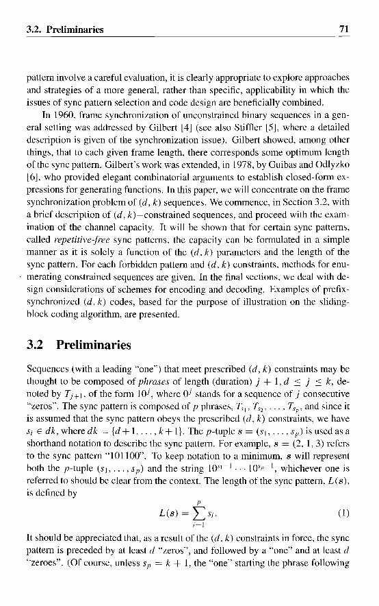
3.2. Preliminaries 71

pattern involve a careful evaluation, it is clearly appropriate to explore approachesand strategies of a more general, rather than specific, applicability in which theissues of sync pattern selection and code design are beneficially combined.

In 1960, frame synchronization of unconstrained binary sequences in a gen­eral setting was addressed by Gilbert [4] (see also Stiffler [5], where a detaileddescription is given of the synchronization issue). Gilbert showed, among otherthings, that to each given frame length, there corresponds some optimum lengthof the sync pattern. Gilbert's work was extended, in 1978, by Guibas and Odlyzko[6], who provided elegant combinatorial arguments to establish closed-form ex­pressions for generating functions. In this paper, we will concentrate on the framesynchronization problem of (d, k) sequences. We commence, in Section 3.2, witha brief description of (d, k)-constrained sequences, and proceed with the exam­ination of the channel capacity. It will be shown that for certain sync patterns,called repetitive-free sync patterns, the capacity can be formulated in a simplemanner as it is solely a function of the (d, k) parameters and the length of thesync pattern. For each forbidden pattern and (d, k) constraints, methods for enu­merating constrained sequences are given. In the final sections, we deal with de­sign considerations of schemes for encoding and decoding. Examples of prefix­synchronized (d, k) codes, based for the purpose of illustration on the sliding­block coding algorithm, are presented.

3.2 Preliminaries

Sequences (with a leading "one") that meet prescribed (d, k) constraints may bethought to be composed of phrases of length (duration) j + 1, d ~ j ~ k, de­noted by Tj+ I, of the fonn IOJ, where oj stands for a sequence of j consecutive"zeros". The sync pattern is composed of p phrases, Tq , TS2 ' ••• , Tsp ' and since itis assumed that the sync pattern obeys the prescribed (d, k) constraints, we haveSi E dk, where dk = {d + 1, ... , k+ I}. The p-tuple s = (s], ... , sp) is used as ashorthand notation to describe the sync pattern. For example, s = (2, 1,3) refersto the sync pattern "101100". To keep notation to a minimum, s will representboth the p-tuple (s I, ... , sp) and the string 10.1'1- 1 ••• lOsp-l, whichever one isreferred to should be clear from the context. The length of the sync pattern, L (s),

is defined byp

L(s) = I>i'i=]

(l)

It should be appreciated that, as a result of the (d, k) constraints in force, the syncpattern is preceded by at least d "zeros", and followed by a "one" and at least d"zeroes". (Of course, unless sp = k + 1, the "one" starting the phrase following

72 3. Prefix-synchronized Runlength-limited Sequences

the sync pattern must be a part of the binary pattern used by the synchronizationcircuitry at the receiver.) It is, therefore, a matter of debate to say that the syncpattern length is L(s) or L(s) + 2d + 1. The adopted definition (1) is slightlymore convenient, as we will see shortly.

Each frame of coded information consists of the prescribed sync pattern sanda string of I cascaded phrases ~1' ••• ,Til' The frame is organized according tothe format

(2)

The total number of binary digits contained in a frame is prescribed and is denotedby Lframe; that is.

p I

Lframe = L s j + L i j . (3)j=l j=l

The valid choices of ~l' ••• , Til are those for which no p consecutive phrasestaken from

(4)

agree with the sync pattern. Dictionaries satisfying this constraint are calledprefix-synchronized runlength-limited codes. It is relevant to enumerate the num­ber of distinct Lframe-tuples given the above conditions. Following this enumer­ation problem, we will deal with a related problem, namely the computation ofthe number of constrained sequences when the frame length Lframe is allowed tobecome very large.

3.3 Enumeration of Sequences

In this section, we will address the problem of counting the number of constrainedsequences. Our methods can be viewed as an extension of those of Guibas andOdlyzko [6] but can, in fact, be traced back to the work of Schuetzenberger onsemaphore codes [7, remark 3], see also Berstel and Perrin, [8, sect. II-7 andnotes following sec. VI]. Schuetzenberger attributes these results to Von Misesand Feller [9]. Related work can be found in [10].

First we develop some notation. Let F be the collection of all sequences T ofthe fOlm

ij E dk, j = 1, ... , n, (5)

composed of n > p phrases of length

n

L(T) = Li j ,

j=l

(6)

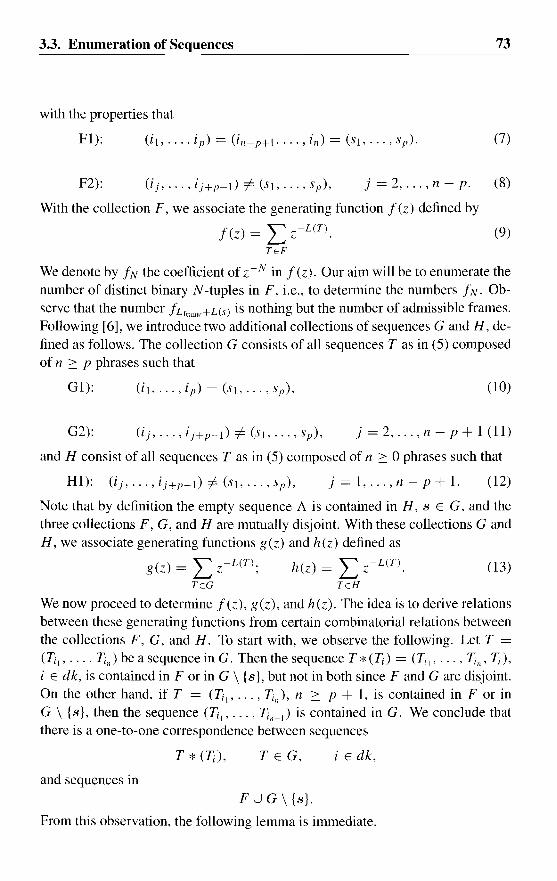
3.3. Enumeration of Sequences

with the properties that

73

F1): (7)

F2): (ij, ... , ij+p_l) =!- (SI, ... , sp), j = 2, ... , n - p. (8)

With the collection F, we associate the generating function fez) defined by

fez) = L Z-L(T). (9)TEF

We denote by iN the coefficient of Z-N in fez). Our aim will be to enumerate thenumber of distinct binary N -tuples in F, i.e., to determine the numbers fN. Ob­serve that the number fLframe+L(S) is nothing but the number of admissible frames.Following [6], we introduce two additional collections of sequences G and H, de­fined as follows. The collection G consists of all sequences T as in (5) composedof n :::: p phrases such that

GI): (10)

G2): (ij, ... , ij+p_l) =!- (Si, ... , Sp), j = 2, ... , n - p + 1 (11)

and H consist of all sequences T as in (5) composed of n :::: 0 phrases such that

HI): (ij, ... ,ij+p-d=!-(sl, ... ,sp), j=I, ... ,n-p+1. (12)

Note that by definition the empty sequence A is contained in H, S E G, and thethree collections F, G, and H are mutually disjoint. With these collections G andH, we associate generating functions g(z) and h(z) defined as

g(z) = L Z-L(T); h(z) = L Z-L(T). (13)TEG TEH

We now proceed to determine fez), g(z), and h(z). The idea is to derive relationsbetween these generating functions from certain combinatorial relations betweenthe collections F, G, and H. To start with, we observe the following. Let T =

('L1, .... TiJ be a sequence in G. Then the sequence T *('L) = (Trl' ... , 'Ln , 'L),i E dk, is contained in F or in G \ {s}, but not in both since F and G are disjoint.On the other hand. if T = ('L 1 , ••• , 'L,), n :::: p + I, is contained in F or inG \ {s}, then the sequence ('L1 , ••• , 'Ln - I ) is contained in G. We conclude thatthere is a one-to-one correspondence between sequences

and sequences in

T * ('L), T E G, i E dk,

FUG\{s}.

From this observation, the following lemma is immediate.

74

Lemma 1:

3. Prefix-synchronized Runlength-limited Sequences

g(Z)Pdk(Z) = fez) + g(z) - Z-L(s),

where

Proof We have

Pdk(Z) = L Z-L(T;) = L Z-i.

iEdk iEdk

(14)

L Z-L(T). L Z-L(Ti)

TEG iEdk

L L Z-UT*(T;))

TEGiEdk

L Z-L(T)

TEFUG,Tf-s

fez) + g(z) - z-Us).

D

Similarly, we may derive a one-to-one correspondence between sequences

and sequences in

CIi) * T, T E H,

HUG \ {i\},

i E dk,

(recall that G and H are disjoint), which leads to the next lemma.

Lemma 2:

Pdk(Z)h(z) = h(z) + g(z) - 1.

Proof Similar to the proof of Lemma 1. (Note that Z-L(A) = zo = 1). D

Before we can write down the last relationship we require some definitions.Define the (p - i)-tuples h(i) = (Sl, , sp-d and t(i) = (Si+l, ... , sp), so

h(i) and t(i) consist of the p - i, i = 0, , p - 1, first and last phrases of themarker s, respectively. Let L(h(i)) be the length of the first p - i phrases of s, or

p-i

L(h(i)) = LSj.j=l

(15)

The autocorrelation function of s, denoted by r, is a binary vector of length pwhich is defined by ri = 0 if h(i) #- t(i) and ri = 1 if h(i) = t(i). Obviously, ro =1. An example may serve to explain why r is termed auto-correlation function.

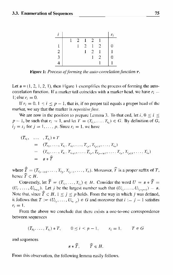
3.3. Enumeration of Sequences

i ri

1 2 1 2 ]

1 1 2 1 2 02 1 2 1 13 1 2 04 1 1

Figure 1: Process offorming the auto-correlation function T.

7S

Let s = (l, 2, 1, 2, 1), then Figure 1 exemplifies the process of forming the auto­correlation function. If a marker tail coincides with a marker head, we have ri =1; elseri = O.

If ri = 0, 1 :::: i :::: p - 1, that is, if no proper tail equals a proper head of themarker, we say that the marker is repetitive free.

We are now in the position to prepare Lemma 3. To that end, let i, 0 :::: i ::::p - 1, be such that ri = 1, and let T = (~l' ... , Tin> E G. By definition of G,i j =Sj for j = 1, ... ,p. Sinceri = 1, we have

(TVl"'" Ts;, TS1 ,"" Tv p ' ~p+l"'" ~n)

(TSI , ... , TSi , TVi+l' ... , Tsp ' TSp_i +I' ... , Tsp ' Tip+l ' ... , Tin>

where T = (TSp_i+I' ... , Tsp ' Tip+l ' ... , Tn). Moreover, T is a proper suffix of T,

hence T E H.

Conversely, let T = (~l"'" ~n> E H. Consider the word U = s * T =(Uil"'" Uin+p) Let j be the largest number such that (Uij"'" Uij+p_l) = s.Note that, since T E H, 1 :::: j :::: p holds. From the way in which j was defined,it follows that T := (Ui j , ... , Uin+p) E G and moreover that i := j - 1 satisfiesri = 1.

From the above we conclude that there exists a one-to-one correspondencebetween sequences

and sequences

o :::: i :::: p - 1, TEG

s * T, T E H.

From this observation, the following lemma easily follows.

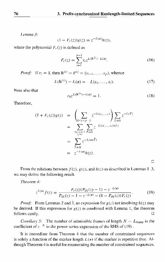
76

Lemma 3:

3. Prefix-synchronized Runlength-limited Sequences

(I + Fr(z))g(z) = z-L(s)h(z),

where the polynomial Fr (z) is defined as

p-I

Fr(z) = LrizL(h(i)-L(S).

i=1

proqr If ri = I, then h(i) = t(i) = (Si+l, ... ,sp), whence

L(h(i») - L(s) = -L(s], ... , Si)'

Note also that

Therefore,

(16)

(17)

(18)

(1 + Fr(z))g(z) ( L Z-LCSI .....SiJ) L z-UT)

O-Si-Sp-I TEG

L L Z-L((SI ......I;)*T)

O.c:i.c:p-! TEGrj=!

L Z-L(s*T1

fER

z-L(s)h(z).

D

From the relations between fez), g(z), and h(z) as described in Lemmas 1-3,we may derive the following result.

Theorem 4:

ZL(s)!(Z) = Fr(Z)(Pdk(Z) - I) - Z-L(s) (19)

Pdk(Z) - 1 - eLls) - (1 - Pdk(Z))Fr(z)

Proof From Lemmas 2 and 3, an expression for g(z) not involving h(z) maybe derived. If this expression for g(z) is combined with Lemma 1, the theoremfollows easily. [J

Corollary 5: The number of admissible frames of length N = Lframe is thecoefficient of eN in the power series expression of the RHS of (19) .

It is immediate from Theorem 4 that the number of constrained sequencesis solely a function of the marker length L (s) if the marker is repetitive free. Al­though Theorem 4 is useful for enumerating the number of constrained sequences,

3.3. Enumeration of Sequences 77

it shows its greatest utility in investigating the asymptotic behaviour of the num­ber of constrained sequences when the sequence length is allowed to become verylarge.

This asymptotic behaviour is directly related to the (noiseless) capacity to bediscussed in the ensuing section.

3.3.1 Capacity

The number of distinct (d, k) sequences of length n, denoted by Ndk(n), grows,for sufficiently large n, exponentially:

(20)

where al is a constant independent of 11, and the rate of growth C(d, k) is termedthe (noiseless) capacity of the (d, k)-constrained channel. The capacity C(d, k)

is the base-210garithm of the largest real root of the characteristic equation [11]

Pdk(Z) = L Z-i = 1.iEdk

For the d-constrained case, k = 00. we have the characteristic equation

00 -d() ,,-i Z 1Pd,oo Z = L Z = -- = .

i=d+l Z - I

(21)

(22)

Using the above characteristic equations, it is not difficult to compute the capacityof (d, k)-constrained channels. The results of the computations have been tabu­lated in [l] .

The capacity C(d, k, s) of (d, k) sequences where the marker s is forbiddencan be found from the next theorem.

Theorem 6: C(d, k, s) = log2 A, where A is the largest real root of

(23)

Proof" Follows from Theorem 4. Note that numerator and denominator of theRHS of (19) have no common factors. 0

An upper and lower bound to the capacity C(d, k, s) are given in the nextcorollary.

Corollary 7: For given sync pattern length L(s),

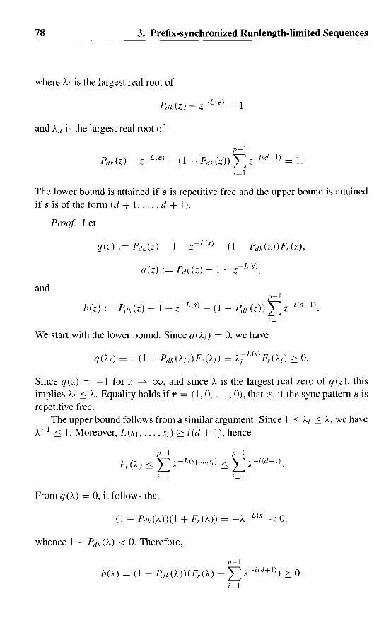
78 3. Prefix-synchronized Runlength-limited Sequences

where Al is the largest real root of

and Au is the largest real root of

p-I

Pdk(Z) - Z-L(s) - (l - Pdk(Z)) I:>-i(d+l) = 1.i=1

The lower bound is attained if 8 is repetitive free and the upper bound is attainedif 8 is ofthe form (d + L ... , d + 1).

Proof Let

q(z) := Pdk(Z) - 1 - Z-L(s) - (1 - P,tk(z))Fr(z),

a(z) := Pdk(Z) - 1 - Z-L(s),

andp-I

b(z) := P,/k(z) - 1 - Z-L(s) - (1 - Pdk(Z» L Z-i(d+1).

i=1

We start with the lower bound. Since a(AI) = 0, we have

Since q(z) = -1 for Z ---7 00, and since A is the largest real zero of q(z), thisimplies Al :::: A. Equality holds if r = (l, 0, ... , 0), that is, ifthe sync pattern 8 isrepetitive free.

The upper bound follows from a similar argument. Since 1 :::: Al :::: A, we haveA-I :::: 1. Moreover, L (s 1, ... , SI) :::: i (d + 1), hence

p-I p-I

Fr(A):::: LA-L(SI, ... ,Si) :::: LA-i(d+IJ.

1=1 1=1

From q(A) = 0, it follows that

(l - Pdk(A»(l + Fr(A» = -A -L(s) < 0,

whence 1 - Pdk(A) < 0. Therefore,

p-l

b(A) = (l - Pdk(A»(Fr(A) - L A-- i(d+1) :::: 0.i=1

3.4. Code Design

Table 1: Capacity of the (1, 3)-constrained channel.

s C(1, 3, s) I: v; max{v;}

1000 .405691010 .4649610100 A5316100010 .48673100100 .50630 18 4101010 .51737 30 61000100 .50902 11 31001010 .50902 20 41010010 .51606 33 610001000 .52934 II 310001010 .52352 12 310010010 .52352 18 410010100 .52785 26 410100010 .52669 32 610101010 .53691 30 6

79

Since b(z) = -1 for z -+ 00, and since Au is the largest real zero of b(z), thisimplies A :::: Au. [J

Tables 1-3 present C(d, k, s) for selected (d, k) parameters. (The right-handcolumns are related to the code design to be discussed in a later section.) FromTable 1 we observe, for example, that s = (3, 3) is the shortest sync pattern thatadmits of a code with rate 1: 2, while the shortest repetitive-free sync patternsthat admit of the same code rate are s =(4, 3) and (3, 2, 2) (and, of course, theirreversed counterparts, which are not in the table). In the Appendix, an analysisis given to approximate C(d, k, s). In the next section, we will discuss what theconsequences are in terms of encoder and decoder complexity.

3.4 Code Design

In this section, we use the preceding theory to provide some examples of codedesign based on the sliding-block code algorithm [12] . The starting point of thesliding-block code algorithm is a description of the channel constraints by a la­beled directed graph. An N~-state (labeled) graph is characterized by an N s x N s

adjacency matrix D with non-negative integer entries and a labeling output func­tion l; that maps the transitions (edges) into the channel alphabet. In the nextsection, we will describe the graph that represents the (d, k) and synchronization

80 3. Prefix-synchronized Runlength-limited Sequences

Table 2: Capacity of the (1, 7) -constrained channel.

s CO, 7, s) ~Vi max{vd1000000 .662621000010 .662621000100 .662621001010 .662621010010 .6642210000000 .66903 99 1910000010 .66903 129 1910000100 .66903 147 1910001000 .67047 164 1910001010 .66903 160 1910010010 .66903 275 3010010100 .66998 252 2710100010 .66965 279 2710101010 .67302 142 15100000010 .67296 65 11100000100 .67296 76 11100001000 .67296 88 11100001010 .67296 86 11100010010 .67296 102 11100010100 .67296 102 11100100010 .67296 156 16100100100 .67448 153 16100101010 .67296 152 16101000010 .67320 198 19101001010 .67320 202 19

constraints. Thereafter, as a straightforward application, we present some exam­ples of code design.

3.4.1 Graph description

We will now proceed to show that the constraints can be represented by an (L +k + 1 - sl)-state graph. Admissible sequences emitted by the graph exclude thesync pattern as well as those sequences which violate the (d, k) constraints. Letthe (L + k + 1 - Sl) states be denoted by 0"1, ... , O"L, 0-1 , ... ,o-k+1-sj' The graphoccupies state O"i, 1 ~ i ~ L, if it is possible to form a marker by extendingthe generated sequence with L - i + 1 symbols, or stated alternatively, if the i

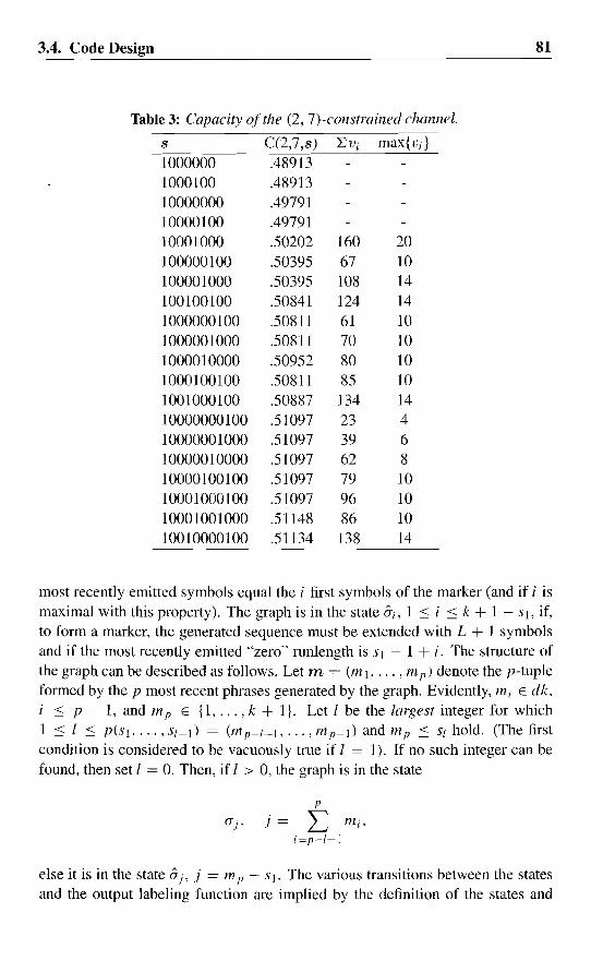
3.4. Code Design

Table 3: Capacity o/the (2, 7)-collstrained channel.

S C(2,7,s) ~Vi max{vd1000000 .489131000100 .4891310000000 .4979110000100 .4979110001000 .50202 160 20100000100 .50395 67 10100001000 .50395 108 14100100100 .50841 124 141000000100 .50811 61 101000001000 .50811 70 101000010000 .50952 80 101000100100 .50811 85 101001000100 .50887 134 1410000000100 .51097 23 410000001000 .51097 39 610000010000 .51097 62 810000100100 .51097 79 1010001000100 .51097 96 1010001001000 .51148 86 1010010000100 .51134 138 14

81

most recently emitted symbols equal the i first symbols of the marker (and if i ismaximal with this property). The graph is in the state Ui, I ~ i ~ k + 1 - S], if,to form a marker, the generated sequence must be extended with L + 1 symbolsand if the most recently emitted "zero" run1ength is s, - 1 + i. The structure ofthe graph can be described as follows. Let m = (m], ... , m p ) denote the p-tup1eformed by the p most recent phrases generated by the graph. Evidently, mi E dk,i ~ P - 1, and m p E {l, ... , k + 1}. Let l be the largest integer for which1 ~ l ~ p(s], ... , Sl-]) = (mp-l+l, ... , mp-I> and m p ~ Sl hold. (The firstcondition is considered to be vacuously true if l = I). If no such integer can befound, then set l = O. Then, if l > 0, the graph is in the state

P

(Jj. j = L mi,i=p-l+]

else it is in the state Uj, j = m p - S]. The various transitions between the statesand the output labeling function are implied by the definition of the states and

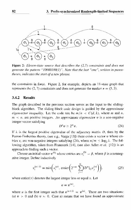
82 3. Prefix-synchronized Runlength-limited Sequences

Figure 2: Eleven-state source that describes the (2,7) constraints and does notgenerate the pattern "10000100(1)". Note that the last "one", written in paren­theses, indicates the start ofa new phrase.

the constraints in force. Figure 2, for example, depicts an II-state graph thatrepresents the (2, 7) constraints and does not generate the marker s = (5,3).

3.4.2 Results

The graph described in the previous section serves as the input to the sliding­block algorithm. The sliding-block code design is guided by the approximateeigenvector inequality. Let the code rate be min < C(d, k), where m and n,m < n, are positive integers. An approximate eigenvector v is a non-negativeinteger vector satisfying

(24)

If A is the largest positive eigenvalue of the adjacency matrix D, then by thePerron-Frobenius theory, (see e.g.. Varga [13]) there exists a vector v whose en­tries Vi are non-negative integers satisfying (24), where nI m S log2 A. The fol­lowing algorithm, taken from Franaszek [14], (see also Adler et al. [12]) is anapproach to finding such a vector.

Choose an initial vector v(O) whose entries are viOl = {J, where (J is a nonneg­ative integer. Define inductively

(25)

where entier(x) denotes the largest integer less or equal x. Let

where u is the first integer such that v(u+l) = v(u). There are two situations:(a) v > 0 and (b) v = O. Case a) means that we have found an approximate

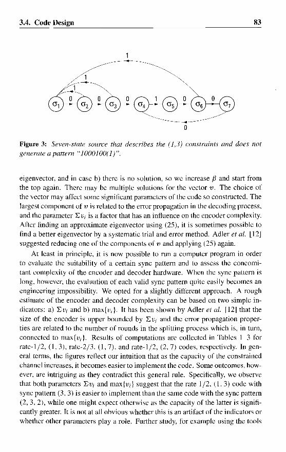
3.4. Code Design

o

83

Figure 3: Seven-state source that describes the (l,3) constraints and does notgenerate a pattern "1000100(1)".

eigenvector, and in case b) there is no solution, so we increase f3 and start fromthe top again. There may be multiple solutions for the vector v. The choice ofthe vector may affect some significant parameters of the code so constmcted. Thelargest component of v is related to the error propagation in the decoding process,and the parameter I; Vi is a factor that has an influence on the encoder complexity.After finding an approximate eigenvector using (25), it is sometimes possible tofind a better eigenvector by a systematic trial and error method. Adler et al. [12]suggested reducing one of the components of v and applying (25) again.

At least in principle, it is now possible to mn a computer program in orderto evaluate the suitability of a certain sync pattern and to assess the concomi­tant complexity of the encoder and decoder hardware. When the sync pattern islong, however, the evaluation of each valid sync pattern quite easily becomes anengineering impossibility. We opted for a slightly different approach. A roughestimate of the encoder and decoder complexity can be based on two simple in­dicators: a) I; Vi and b) max{Vi}. It has been shown by Adler et al. [12] that thesize of the encoder is upper bounded by L;Vi and the error propagation proper­ties are related to the number of rounds in the splitting process which is, in tum,connected to max{vd. Results of computations are collected in Tables 1-3 forrate-I/2, (1,3), rate-2j3, (1,7), and rate-l 12, (2,7) codes, respectively. In gen­eral terms, the figures reflect our intuition that as the capacity of the constrainedchannel increases, it becomes easier to implement the code. Some outcomes, how­ever, are intriguing as they contradict this general mle. Specifically, we observethat both parameters I; Vi and max{vd suggest that the rate 1/2, (1, 3) code withsync pattern (3, 3) is easier to implement than the same code with the sync pattern(2,3,2), while one might expect otherwise as the capacity of the latter is signifi­cantly greater. It is not at all obvious whether this is an artifact of the indicators orwhether other parameters playa role. Further study, for example using the tools

84 3. Prefix-synchronized Runlength-Iimited Sequences

Table 4: Code book ofrate 1/2. (1, 3) code.

a; g(a;, O) !lea;, 0) g(a;.I) !l(a;, 1)

1 1 10 4 102 1 00 5 003 2 01 3 014 1 00 3 105 3 01 3 10

presented by Marcus and Roth [15], is needed to answer these questions. In thenext section. we will describe a worked example of the design of a rate 112, (1. 3)code.

3.4.3 Worked example

We consider the design of a rate 1/2, (1,3) code which does not generate themarker s = (4.3) or "1000100(1)". The capacity of the channel is (see Ta­ble 1) CO, 3, S = (4,3)) = 0.50902, so that this code achieves an efficiency of0.5/0.50902 = 98.2%. Figure 3 shows the graphical representation of a seven­state source whose output sequences obey the given constraints.

The adjacency matrix D associated with this source is

0 1 0 0 0 0 01 0 1 0 0 0 01 0 0 1 0 0 0

D= 0 0 0 0 1 0 0 (26)

0 0 0 0 0 1 01 0 0 0 0 0 10 0 0 1 0 0 0

Invoking (25), we find the approximate eigenvector v T = (2,3,2,1,1,2,0).After the previous spadework, it is now a simple matter to assemble, using thesliding-block coding algorithm, a rate 1/2, (1,3) sliding-block encoder. The en­coder is defined by two characterizing functions: the next-state function g (a;, /3/1)

and the output function h(a;. ~u), where ~u, u = 1, ... , 2m , are the 2m sourcewords, and (i;. i = 1.... , Ne , are the Ne encoder states. The output and next-statefunction are shown in Table 4.

The implementation of the rate 1/2, (1, 3) encoder is elementary; the encodercomprises a three-stage register to store the actual state (three bits are sufficient torepresent the five encoder states). and a (l +3) ----+ (2+3) logic array for lookingup the 2-b codeword and the 3-b next-state. Decoding can be accomplished by a

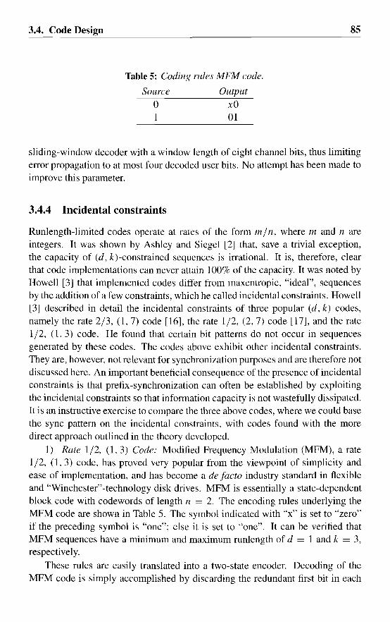
3.4. Code Design

Table 5: Coding rules MFM code.

Source Output

o xO1 01

85

sliding-window decoder with a window length of eight channel bits, thus limitingerror propagation to at most four decoded user bits. No attempt has been made toimprove this parameter.

3.4.4 Incidental constraints

Runlength-limited codes operate at rates of the form min, where m and n areintegers. It was shown by Ashley and Siegel [2] that, save a trivial exception,the capacity of (d, k)-constrained sequences is irrational. It is, therefore, clearthat code implementations can never attain 100% of the capacity. It was noted byHowell [3] that implemented codes differ from maxentropic, "ideal", sequencesby the addition of a few constraints, which he called incidental constraints. Howell[3] described in detail the incidental constraints of three popular (d, k) codes,namely the rate 2/3, (l, 7) code [16], the rate 1/2, (2,7) code [17], and the rate1/2, (l, 3) code. He found that certain bit patterns do not occur in sequencesgenerated by these codes. The codes above exhibit other incidental constraints.They are, however, not relevant for synchronization purposes and are therefore notdiscussed here. An important beneficial consequence of the presence of incidentalconstraints is that prefix-synchronization can often be established by exploitingthe incidental constraints so that infornlation capacity is not wastefully dissipated.It is an instructive exercise to compare the three above codes, where we could basethe sync pattern on the incidental constraints, with codes found with the moredirect approach outlined in the theory developed.

1) Rate 1/2, (l, 3) Code: Modified Frequency Modulation (MFM), a ratel/2, (l, 3) code, has proved very popular from the viewpoint of simplicity andease of implementation, and has become a de facto industry standard in flexibleand "Winchester"-technology disk drives. MFM is essentially a state-dependentblock code with codewords of length n = 2. The encoding rules underlying theMFM code are shown in Table 5. The symbol indicated with "x" is set to "zero"if the preceding symbol is "one"; else it is set to "one". It can be verified thatMFM sequences have a minimum and maximum runlength of d = 1 and k = 3,respectively.

These rules are easily translated into a two-state encoder. Decoding of theMFM code is simply accomplished by discarding the redundant first bit in each

86 3. Prefix-synchronized Runlength.limited Sequences

received 2-b block. It is not difficult to check that under MFM rules, the outputsequence ., 10 00" is not valid, but "01 00 01", however, is valid, so that"1000"cannot serve as a sync pattern. The shortest sequence that does not occur in anMFM sequence is the 12-b sequence "100010010001". Perusal of Table J revealsthat the shortest markers giving room for the design of a rate 1/2 code are oflength six. The rate 1/2, (l, 3) code described in Section 3.4.3 has the advantagethat its sync word is 8-b long instead of twelve bits required in the MFM code.On the other hand, the MFM code has a simpler implementation and the decoderwindow length is shorter, namely two bits, and is thus more favorable in terms oferror propagation.

2) Rate 1/2, (2,7) Code: A great many kinds ofrate-l/2 codes are knownfor the parameters d = 2 and k = 7. We will concentrate on the variable-lengthvariant invented by Franaszek [17] and modified by Eggenberger and Hodges [18].The code can be encoded with a six-state encoder (Howell [3] showed how todevise a five-state encoder) and decoded with a sliding-block decoder of lengtheight. Howell [3] found that this (2, 7) code does not produce 12-b sequences ofthe form 107 102 1, so that the sequence s = (8, 3) can be used as a marker in thisscheme. In Table 3, we observe that there are nine candidate sync patterns s oflength L (s) < 11 which permit the construction of a rate 1/2 code; the shortestmarker has length eight. Rate-l/2 codes which embed each of these candidatemarkers were generated using the sliding-block coding algorithm. Approximately10 rounds of splitting steps are required for the codes with the markers of length 8and 9: the corresponding encoders utilize approximately 30 states. The codes forthe markers of length 10 require 8 splitting rounds. The simplest code found usesthe marker s = 0,3); the code requires 23 encoder states and can be decodedwith a decoder window of 23 bits.

3) Rate 2/3, (1, 7) Code: The rate 2/3, (1, 7) code described by Jacobyand Kost [16] is a lookahead code. It can be encoded by a five-state encoder anddecoded by a decoder with a window of seven bits. Howell [3] has observed thatthe set of sequences generated by this code is invariant under time reversal. The16-b pattern 106 107 1 and its reverse 107 106 1 do not occur in sequences generatedby the (1. 7) code. We have evaluated a number of shorter sync patterns, but couldnot find a code that rivaled the Jacoby/Kost code in complexity.

3.5 Conclusions

We have investigated the prefix-synchronization of runlength-limited sequences.In particular, we have analyzed the capacity of (d, k)-constrained channels givingroom for the prefix-synchronization fonnat. It has been shown that for certain

Appendix: Approximations to the capacity 87

sync patterns, termed repetitive-free sync patterns, the capacity can be formulatedin a simple manner, as it is solely a function of the (d, k) parameters and the lengthof the sync pattern. For presentation purposes, the complexity consequences ofshort sync patterns have been investigated for the rate-l /2 codes with parameters(1,3) and (2,7), and for the rate 2/3, (1,7) code. We have not found a codethat rivaled the (1, 7) and (2, 7) codes whose sync patterns are based on theirrespective incidental constraints. A worked example of a rate 1/2, (l, 3) codegiving room for the inclusion of a unique sync pattern of length seven has beenpresented.

Appendix: Approximations to the capacity bounds

In this Appendix, we derive approximations to the lower and upper bound tothe capacity C(d, k, s). Corollary 7 asserts that for given marker length L(s),log2 Al ::::: C(d, k, s) ::::: log2 Au, where Al is the largest real root of

P,/k(z) - Z-L(s) = 1

and Au is the largest real root of

1'-1

Pdk(Z) - Z-L(s) - (1 - Pddz)) L Z~i(d+1) = 1.i=]

We commence with the lower bound. To that end, let fL be the largest real root ofthe characteristic equation

Pdk(Z) = L Z-i = 1iEdk

and let Al = fL + D.AI be the largest real root of

Pdk(Z) - Z-L(s) = 1.

ThenPdk(fL + D.AI) - (fL + D.Af}-L(s) = 1.

Differentiating and working out yields

D.AI ::::::: - fL fL -L(s)T

where the average runlength T is

T=LifL- i .iEdk

L(s) » 1,

88 References

Thus,

C(d, k, s) > log2(f.L + !~)"'l)

C(d, k) + log2(1 + !:J.Ai/ f.L)

IC(d, k) - f.L-L(S).

In(2)T

In a similar fashion, we find for the upper bound Au = f.L + !:J.Au :

f.L -L(s)

p-I

1 + Lf.L-i(d+l)

i=l

f.L------

T

We havep-I 1

1 + '"' f.L -i (d+I) ::::::: __-----,--,----,-6. I - f.L-(d+lJ'

and from (22) we infer that, for k » I,

L(s)>>I,

fJ-ld+1) I -I- f.L ,

so that1

!:J.Au ::::::: - = f.L -L(s),

TL(s) »L k» I.

Thus, for the relative capacity loss we find the following approximations:

1 I-- f.L-L(s)-1 < C(d, k) - C(d, k, s) < f.L- LlsJ •

In(2)T In(2)TL(s) » I.

References

[1] K.A.S. Immink, "Runlength-Limited Sequences", Proc. IEEE, vol. 78, no.11, pp. 1745-1759, Nov. 1990.

[2] J. Ashley and P.H. Siegel, "A Note on the Shannon Capacity of Run-Length­Limited Codes", IEEE Trans. Inform. Theory, vol. IT-33, no. 4, pp. 601-605,July 1987.

[3] T.D. Howell, "Statistical Properties of Selected Recording Codes", IBM J.Res. Develop., vol. 33, no. 1, pp. 60-73, Jan. 1989.

[4] E.N. Gilbert, "Synchronization of Binary Messages". IEEE Trans. Inform.Theory, vol. IT-6, no. 5, pp. 470-477, Sept. 1960.

References 89

[5] J.J. Stiffler, Theory of Synchronous Communications, Enge1wood Cliffs:Prentice-Hall, 1971.

[6] LJ. Guibas and AM. Od1yzko, "Maximal Prefix-Synchronized Codes",SIAM J. Appl. Math., vol. 35, no. 2, pp. 401-418, 1978.

[7] M.P Schuetzenberger. "On the Synchronizing Properties of Certain PrefixCodes", Inform. Contr., vol. 7, pp. 23-36, 1964.

[8] J. Berstel and D. Perrin, Theory of Codes, Orlando: Academic Press, 1985.

[9] W. Feller. An Introduction to Probability Theory and Its Applications, Vol­ume I, New York: Wiley, 1959.

[10] D. Lind, "Perturbations of shifts of finite type", Siam J. Disc. Math., vol. 2,pp. 350-365, 1989.

[11] C.E. Shannon, "A Mathematical Theory of Communication", Bell Syst. Tech.J., vol. 27, pp. 379-423, July 1948.

[12] RL. Adler, D. Coppersmith, and M. Hassner, "Algorithms for Sliding BlockCodes. An Application of Symbolic Dynamics to Information Theory",IEEE Trans. Inform. The01Y, vol. IT-29. no. 1, pp. 5-22, Jan. 1983.

[13] R.S Varga, Matrix Iterative Analysis, Enge1wood Cliffs: Prentice-Hall, 1962.

[14] PA Franaszek, "Construction of Bounded Delay Codes for Discrete Noise­less Channels". IBM J. Res. Develop., vol. 26, no. 4, pp. 506-514, July 1982.

[15] B.H. Marcus and RM. Roth, "Bounds on the Number of States in EncoderGraphs for Input-constrained Channels", IEEE Trans. Inform. Theory, vol.IT-37, no. 3, pp. 742-758, May 1991.

[16] G.Y. Jacoby and R Kost, "Binary Two-thirds Rate Code with Full WordLook-Ahead", IEEE Trans. Magnet., vol. MAG-20, no. 5, pp. 709-714,Sept. 1984; see also M. Cohn, G.Y. Jacoby, and C.A. Bates III, U.S. Patent4,337,458, June 1982.

[17] P.A Franaszek, "Run-length-limited Variable Length Coding with ErrorPropagation Limitation", U.S. Patent 3,689,899, Sept. 1972.

[18] J.S. Eggenberger and P. Hodges, "Sequential Encoding and Decoding ofVariable Word Length, Fixed Rate Data Codes", U.S. Patent 4,115,768,1978.

Chapter 4

On the construction ofbounded-delay encodable codesfor constrailled systems

Abstract- We present a new technique to construct sliding-block modulationcodes with a small decoding window. Our method, which involves both state splittingand look-ahead encoding, crucially depends on a new, "local" construction methodfor bounded-delay codes. We apply our method to construct several new codes, allwith a smaller decoding window than previously known codes for the same con­straints at the same rate.

Index Terms - Bounded-delay code, local encoder structure, ACH algorithm,look-ahead coding, state splitting.

4.1 Introduction

In various applications it is desirable to translate or encode sequences of sourcedata into sequences that obey certain constraints. For example, storage systemsbased on magnetic and optical disks and tapes often employ (d, k)-constrainedsequences, binary sequences in which any tW? consecutive "ones" are separatedby at least d and at most k "zeroes". (See e.g. [15], [21].) In most cases ofpractical interest, the collection of allowable sequences, the constrained system,can be described by a finite-state transition diagram (FSTD), a labeled digraph

© 1995, IEEE. Reprinted, with permission, from IEEE Transactions on Information Theory,vol. 41, no. 5, pp. 1354-1378, September 1995.

The material in this paper was presented in part at the IEEE Symposium on Information Theory,Trondheim, Norway, 1994.

92 4. Construction of bounded-delay encodable codes

consisting of a finite number of states and a finite number of transitions betweenstates, each labeled with a code word. The constrained system represented orgenerated by the FSTD consists of all sequences that result by reading off thelabels from the transitions that make up a directed path or walk in the FSTD.

A (modulation) code for a constrained system consists of an encoder, a one­to-one map that transforms sequences of source symbols into allowable sequences,together with a decoder, the inverse of the encoder map. In practical applicationsthe encoder takes the form of a synchronous finite-state machine. Such a deviceaccepts arbitrary source symbols from a given source alphabet B as input, andproduces a code word depending on this input and the current state of the encoder.(Such codes are called synchronous.) Typically, each source symbol is made upof p user bits, and each code word is composed of q channel bits, for some fixednumbers p and q. The number p / q is called the (binary) rate of the code.

Since modulation codes are normally used in a noisy environment, it is impor­tant that the decoder limits the propagation of input errors. All codes consideredin this paper will have a sliding block decoder. Such a decoder retrieves the orig­inal source symbol at the input of the encoder from the corresponding code wordalong with a fixed number m of preceding code words and a fixed number a ofsubsequent code words. We refer to these m + I + a code words as the decodingwindow for this source symbol, and we say that the code has a decoding-windowsize of m + 1 + a code words. Note that a single error in the input to a sliding­block decoder affects at most m + I + a source symbols, so the amount of errorpropagation (the maximum number of erroneous bits in the output sequence pro­duced by the decoder caused by a single bit error at the input) remains bounded.The decoding-window size also has a direct bearing on the amount of hardwareneeded to implement the decoder. For these reasons, it is an important parameterof a code and should be as small as possible.

Throughout the years, various code construction methods have been devised.The effectivity of these methods depends (amongst others) on the desired rate p / qof the code. In this paper we concentrate on methods which are most effectivewhen p and q are relatively small. (For a more general overview, see e.g. [15].) Aclassical technique is the Bounded-Delay (BD) method developed by Franaszekin a sequence of papers [6], [7], [8], [9]. This method constructs codes that em­ploy look-ahead encoding (or, equivalently, involve an encoding delay) and aimsto minimize the decoding window. A drawback of the BD method is that codeconstruction may involve large and complex search problems. A breakthroughoccurred with the discovery of the ACH state splitting algorithm [2]. This algo­rithm, which in its simplest form is polynomial-time and of low complexity, isguaranteed to produce a code for a constrained system of finite type, at any (ra­tional) rate not exceeding the Shannon capacity of the constraint. However, the

4.1. Introduction 93

method allows a great deal of freedom of choice and it is far from evident how touse this freedom to obtain a code with a small decoding window.

Both the BD method and the ACH algorithm produce codes for a given con­strained system by transforming a given FSTD that represents these constraints.Moreover, in both cases the transformations are guided by an approximate eigen­vector that assigns certain weights to the states of the given FSTD. The ACHalgorithm does so by a process called (forward) state splitting. Here, a (forward)state split essentially subdivides a state by partitioning the set of transitions leav­ing that state. Our description of BD codes in Section 3 shows that the BD-methodmay be considered as bachvard state splitting, where states are now subdividedby partitioning the set of transitions entering a state. We will refer to these trans­formations by saying that states are subdivided according to their future (as in theACH algorithm) or to their history (as in the BD-method).

In this paper, we propose a code construction technique that combines aspectsof these two methods, generalizing the approach in [17]. The method aims specif­ically at the design of codes with a small decoding window. The constructioninvolves both state splitting and look-ahead encoding (thus subdivides states ac­cording to both future and history), and is again guided by an approximate eigen­vector. Our technique crucially depends on a new construction method for BDcodes from what we call a local encoder structure. This method allows the de­composition of the difficult global code construction problem into a number ofindependent, relatively easy, local problems, one for each state.

The existence of a valid encoder structure in a given state (whose constructionmakes up the said local problem for this state) depends only on the weights as­signed to this state and its successors. In particular, if all weights are "sufficientlysmall", then a local encoder structure can always be found. However, it may hap­pen that for some states no valid encoder structure exists. In that case, we reducethe state-weights by state splitting operations. where the state splitting process isdriven by the requirement that a local encoder structure can be formed in each ofthe states. As in the ACH algorithm, we strive to keep the number of rounds ofstate splitting (see e.g. [19]) as small as possible, since this number has a directbearing on the size of the decoding window of the resulting code.

Once we have obtained a complete local encoder structure, it is fairly easyto construct the required BD code. In fact, this construction still atlords somefreedom of choice, which we can employ to minimize the decoding window anderror propagation of the resulting code. Only at this point the specific code wordlabeling of the FSTD is taken into account.

In all examples that we consider (and some of these involve fairly complexconstraints), the appropriate choice of state splitting operations is fairly evident.However, we do not offer a clear-cut algorithm on which to base these choices.

94 4. Construction of bounded-delay encodable codes

Nevertheless, since our technique can be considered as an extension of ACH, anysequence of valid state splittings will eventually produce a code whenever ACHwould. In our view, the method is best implemented interactively; the user choosesthe state splits but the remainder of the work is left to the computer program.

Our method would not be very exciting if the required amount of state splittingwas comparable to that required in straightforward ACH. Fortunately, this doesnot seem to be the case. Indeed, the motivation behind this method stems from thefollowing remarkable observation. An encoder produced from the ACH algorithmby M rounds of state splitting (i.e. M future transitions are taken into account) hasa decoding window of size M +c, for some constant c depending only on the actuallabeling of the FSTD. But sometimes it may happen that decoding requires onlythe K + c last code words from the decoding window, for some K < M. (Anextreme example of this behaviour occurs for bounded-delay encodable, block­decodable (BDB) codes [12], where K = 1 and M can be arbitrarily large. Thiswill be explained elsewhere.) In other words, the effective window size may bemuch smaller than the ordinary window size. (For this reason the lower bound onthe decoding-window size in [18] has to be applied with care.) We will refer to thisproperty by saying that the code has the reduced window property. At first sight,coaching ACH into producing a code with the reduced window property seemsdifficult: the algorithm allows much freedom and there is no evident criterium onwhich to base the choice of the state splitting steps. Is there a way to profit fromthis phenomenon in a systematic way? We will show that in the case describedabove, our code construction technique would require at most K rounds of statesplitting (and often much less) to produce a shifted version of the ACH code, i.e.,corresponding code sequences are equal up to a fixed shift.

In practice, our method performs very satisfactorily, as is witnessed by manyexamples. In particular, in this paper we derive the following new codes:- A rate-2/3 (d, k) = (1, 6)-constrained code with decoding-window size of 5symbols (in fact, only 14 bits), with an error propagation of only 9 bits. (To thebest of our knowledge, the previous record is held by a code described in [1],which has an error propagation of II bits.)- A rate-2lS (d, k, s) = (2, 18, 2)-code, with a decoding-window size of 3 sym­bols. (The previous record was 4 symbols, see [19].)- A rate-2/3 (d. k) = (L 9)-constrained code with a decoding-window of size 2symbols or 6 bits.All of these codes were constructed by hand in a few hours. Moreover, manyknown good codes can also be found by our method, often with surprising ease.

Finally, we observe that our approach allows a uniform description to be givenof various code construction methods such as ACH [2], BD method [8], variablelength codes, prefix-free list codes, variable-length state splitting [3], [11], and a

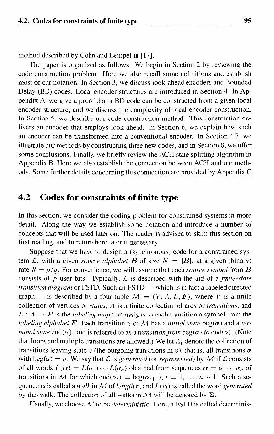
4.2. Codes for constraints of finite type 95

method described by Cohn and Lempel in [17].The paper is organized as follows. We begin in Section 2 by reviewing the

code construction problem. Here we also recall some definitions and establishmost of our notation. In Section 3, we discuss look-ahead encoders and BoundedDelay (BD) codes. Local encoder structures are introduced in Section 4. In Ap­pendix A, we give a proof that a BD code can be constructed from a given localencoder structure, and we discuss the complexity of local encoder construction.In Section 5, we describe our code construction method. This construction de­livers an encoder that employs look-ahead. In Section 6, we explain how suchan encoder can be transformed into a conventional encoder. In Section 4.7, weillustrate our methods by constructing three new codes, and in Section 8. we offersome conclusions. Finally, we briefly review the ACH state splitting algorithm inAppendix B. Here we also establish the connection between ACH and our meth­ods. Some further details concerning this connection are provided by Appendix C

4.2 Codes for constraints of finite type

In this section, we consider the coding problem for constrained systems in moredetail. Along the way we establish some notation and introduce a number ofconcepts that will be used later on. The reader is advised to skim this section onfirst reading, and to return here later if necessary.

Suppose that we have to design a (synchronous) code for a constrained sys­tem £', with a given source alphabet B of size N = IBI, at a given (binary)rate R = p / q. For convenience, we will assume that each source symbol from Bconsists of p user bits. Typically, £, is described with the aid of a finite-statetransition diagram or FSTD. Such an FSTD - which is in fact a labeled directedgraph - is described by a four-tuple M = (V, A, L, F), where V is a finitecollection of vertices or states, A is a finite collection of arcs or transitions, andL : A r-+ F is the labeling map that assigns to each transition a symbol from thelabeling alphabet F. Each transition a of M has a initial state beg(a) and a ter­minal state end(a), and is referred to as a transition from beg(a) to end(a). (Notethat loops and multiple transitions are allowed.) We let A v denote the collection oftransitions leaving state v (the outgoing transitions in v), that is, all transitions a

with beg(a) = v. We say that £, is generated (or represented) by M if £, consistsof all words L(a) = L(a)) ... L(an) obtained from sequences Q = al ... an oftransitions in M for which end(ai) = beg(ai+)), i = 1, ... , n - 1. Such a se­quence Q is called a walk in M of length n, and L (a) is called the word generatedby this walk. The collection of all walks in M will be denoted by ~.

Usually, we choose M to be deterministic. Here, a FSTD is called determinis-

96 4. Construction of bounded-delay encodable codes

tic if in each state the outgoing transitions cany distinct labels. (Any given FSTDthat presents £ can easily be transformed into a deterministic presentation for 12.)

Moreover, it is common practice to choose M to be the Shannon cover, the(unique) deterministic presentation with the minimum number of states. Any givendeterministic FSTD that presents £ can easily be transformed into the Shannoncover by a process called state merging. Here, if the outgoing transitions in twostates can be paired off in such a way that the two transitions in each pair carrythe same label and end in the same state, then from the point-of-view of sequencegeneration these states accomplish the same, hence they can as well be combined,or merged as it is usually called, into a single state. (Note that the resulting FSTDwill again be deterministic.) This process of merging states is repeated until nomore merging is possible. It can be shown that the resulting FSTD, the Shannoncover, does not depend on the order in which the merging was canied out, andthat, moreover, no deterministic FSTD presenting the same constrained systemcan have fewer states, and must be equal to the Shannon cover if it has the samenumber of states. Nevertheless, in what follows, we do not yet make any specialassumptions about the FSTD M chosen to presents the constrained system 12,except that we require that M contains no sources and no sines, i.e., we requirethat each state of M can both be entered and left.

The said coding problem for £ requires that we translate or encode arbitrarysequences of p-bit source symbols into sequences of q-bit code words, where theresulting sequence is required to be in 12, that is, can be generated by some walkin ."'1. Usually the code word size q is a multiple of the size q\ of the labelingsymbols in F, say q = nq\. (Typically, F = {a, I}, ql = I, and n = q.)Therefore it is desirable to have a representation for £ where the labeling symbolsare actually code words. Such a representation is provided by the nth order powergraph Mn of M. This FSTD has the same states as M, but the transitions arenow walks of length n in M; a walk a = a\ ... an is considered as a transitionin M n from state beg(a) = beg(ad to state end(a) = end(an ), and is labeledwith the code word L(a) generated by a. So after replacing M by an appropriatepower graph, we may assume that the labels of M are actually q-bit code words,and now the encoding problem is to transform an arbitrary source sequence into asequence of code words that can be generated by some walk in M.

Commonly, an encoder for £ can actually be put into the form of an encoderfor ~, the collection of walks in M. That is, we may think of the encoder asactually producing the walk that generates the sequence of code words, instead ofthe sequence itself. (We observe that ~ is also a constrained system; indeed, Mrepresents ~ if L is taken to be the identity map.) Note that an encoder for ~produces a transformation from source sequences into sequences of £ through thelabeling map L.

4.2. Codes for constraints of finite type 97

However, some restriction on L is required to ensure that this transformationis actually a code, that is, that decoding is possible. The proper requirement isthat Lis offinite type: there are numbers m and a, the memory and anticipation,respectively, such that walks (Lm ... Q:'o ... Q:'a that generate a given code wordsequence f-m ... fo ... fa all agree in transition Q:'o. If this is the case, then wecan reconstruct the walk Q:'-m ... Q:'o ... Q:'n+a used to generate a given sequencef -m ... fo ... fn+a in 1:, except for the first m and last a transitions. Indeed, notethat each transition Q:'k, 0 ::: k ::: n, is uniquely determined by fk-m ... fk ... fk+a,the decoding window for Q:'k.

In the context of encoder maps, a map of this type is termed sliding-block de­codable, with decoding-window size m + 1 + a and window (m, a). The use ofthe term "finite type" for such a labeling is not standard, but we prefer it becauseit avoids the suggestion that source symbols are to be recovered instead of transi­tions. We also introduce the notion of a map of almost-finite type; the definition issimilar to the one for finite type, except that now we also provide the initial stateof the transition Q:'o to be recovered.

It is well-known that I: is of finite type (i.e. I: can be generated by an FSTD offinite type) precisely when I: can be specified in terms of a finite list offorbiddenblocks [2]. It can also be shown that I: is of almost-finite type (see e.g.[19])precisely when I: can be generated by a deterministic FSTD of almost-finite type[16]. Since the process of state merging referred to above does not destroy eitherof these properties, it follows that I: is of (almost-) finite type if and only if itsShannon cover is of (almost-) finite type. (Indeed, it is not difficult to show that Mis of almost-finite type if and only if M has both finite local memory and finitelocal anticipation. For a definition of these notions, we refer to [19].)

It can be shown that a synchronous code for a constrained system I: repre­sented by an FSTD M of (almost-) finite type. that is, with a labeling of (almost-)finite type, can always be transformed into one arising from a code for ~. (Thistransformation may cause a fixed amount of encoding delay, or equivalently, mayrequire a fixed amount of look-ahead, at the encoder.) It is important to note thatif the labeling map L of M is of finite type and the code for ~ is sliding-blockdecodable, then the corresponding code for I: is again a sliding-block code. (In­deed, note that each successive recovery operation causes only a limited loss ofinformation at both ends of the recovered sequence.) So for most purposes, wecan simply forget about the particular labeling L of M as long as L is of finitetype, and concentrate on constructing a code for ~.

Typically, to construct a code for ~, the FSTD M is first transformed intoanother FSTD M* that is more suitable for encoding purposes, where the trans­formation is such that M* = (V*, A*, L*, A) generates ~, through a map L* offinite type that assigns to each transition Q:'* in M* its parent transition in M.

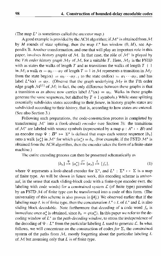
98 4. Construction of bounded-delay encodable codes

(The map L * is sometimes called the ancestor map.)A good example is provided by the ACH algorithm; if M* is obtained from M

by M rounds of state splitting, then the map L * has window (0, M), see Ap­pendix B. Another transformation, and one that will play an important role in thispaper, involves history graphs of M. In that case, the rOle of M* is played bythe Tth order history graph M T of M, for a suitable T. Here, MT is the FSTDwith as states the walks of length T and as transitions the walks of length T + Iin M; a walk 0: = ao· .. aT of length T + I in M represents a transition in MTfrom the state beg(o:) = ao··· aT-l to the state end(o:) = al ... aT, and haslabel L *(0:) = aT. (Observe that the graph underlying M T is the Tth orderedge graph M [TJ of M; in fact, the only difference between these graphs is thata transition 0: as above now carries label L *(0:) = ao. Walks in these graphsgenerate the same sequences, but shifted by T + I symbols.) While state splittingessentially subdivides states according to their future, in history graphs states aresubdivided according to their history, that is, according to how states are entered.(See also Section 3.)

Following such preparations, the code-construction process is completed bytransforming M* into a (look-ahead) encoder (see Section 3): the transitionsof M* are labeled with source symbols (represented by a map cp : A* 1--+ B) andan encoder map \lJ : B* 1--+ b* is defined that maps each source sequence {bn }

onto a walk {a~} in M* for which cp(a~) = bn . (For example, ifthe FSTD M* isobtained from the ACH algorithm, then the encoder takes the form of a finite-statemachine.)

The entire encoding process can then be presented schematically as

(1)

where \lJ represents a look-ahead encoder for b*, and L * : b* 1--+ b is a mapof finite type. As will be shown in future work, this encoding scheme is univer­sal, in the sense that each sliding-block code with a finite-type encoder (wrt. thelabeling with code words) for a constrained system I: (of finite type) presentedby an FSTD M of finite type can be transformed into a code of this form. (Theuniversality of this scheme is also proven in [4].) We observed earlier that if thelabeling map L is of finite type, then the concatenation L * 0 L of L * and L is alsosliding-block decodable. Note furthermore that decoding of a code word fn isimmediate once a~ is obtained, since bn = cp(a~). In this paper we refer to the de­coding window of L * as the path-decoding window, to stress the independence ofthe decoding of \lJ 0 L * from the particular labeling L used to generate 1:. In whatfollows, we will concentrate on the construction of codes for b, the constrainedsystem of the paths from M, mostly forgetting about the particular labeling Lof M but assuming only that L is of finite type.

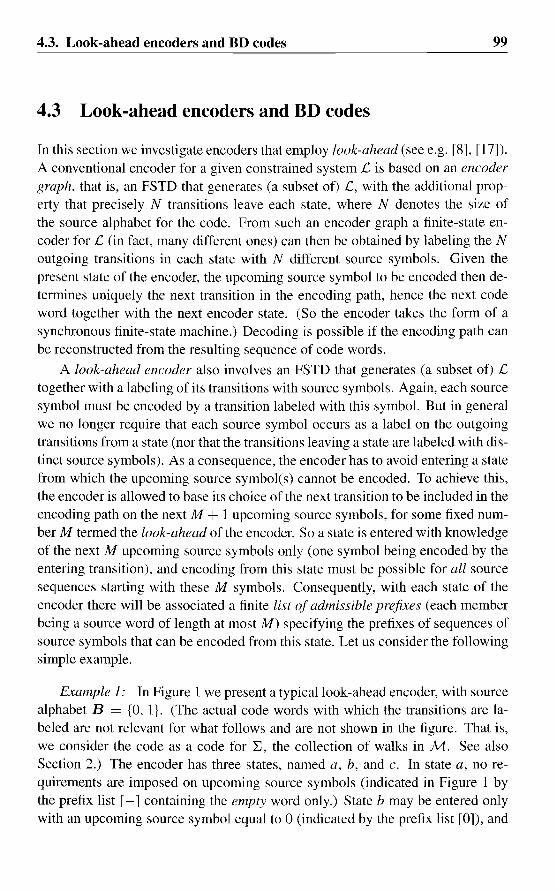
4.3. Look-ahead encoders and BD codes

4.3 Look-ahead encoders and BD codes

99

In this section we investigate encoders that employ look-ahead (see e.g. [8], [17]).A conventional encoder for a given constrained system £ is based on an encoder

graph, that is, an FSTD that generates (a subset of) £, with the additional prop­erty that precisely N transitions leave each state, where N denotes the size ofthe source alphabet for the code. From such an encoder graph a finite-state en­coder for £ (in fact, many different ones) can then be obtained by labeling the Noutgoing transitions in each state with N different source symbols. Given thepresent state of the encoder, the upcoming source symbol to be encoded then de­termines uniquely the next transition in the encoding path, hence the next codeword together with the next encoder state. (So the encoder takes the form of asynchronous finite-state machine.) Decoding is possible if the encoding path canbe reconstructed from the resulting sequence of code words.

A look-ahead encoder also involves an FSTD that generates (a subset of) £together with a labeling of its transitions with source symbols. Again, each sourcesymbol must be encoded by a transition labeled with this symbol. But in generalwe no longer require that each source symbol occurs as a label on the outgoingtransitions from a state (nor that the transitions leaving a state are labeled with dis­tinct source symbols). As a consequence, the encoder has to avoid entering a statefrom which the upcoming source symbol(s) cannot be encoded. To achieve this,the encoder is allowed to base its choice of the next transition to be included in theencoding path on the next M + 1 upcoming source symbols, for some fixed num­ber M termed the look-ahead of the encoder. So a state is entered with knowledgeof the next M upcoming source symbols only (one symbol being encoded by theentering transition), and encoding from this state must be possible for all sourcesequences starting with these M symbols. Consequently, with each state of theencoder there will be associated a finite list of admissible prefixes (each memberbeing a source word of length at most M) specifying the prefixes of sequences ofsource symbols that can be encoded from this state. Let us consider the followingsimple example.

Example 1: In Figure 1 we present a typical look-ahead encoder, with sourcealphabet B = {a, I}. (The actual code words with which the transitions are la­beled are not relevant for what follows and are not shown in the figure. That is,we consider the code as a code for ~, the collection of walks in M. See alsoSection 2.) The encoder has three states, named a, b, and c. In state a, no re­quirements are imposed on upcoming source symbols (indicated in Figure 1 bythe prefix list [-] containing the empty word only.) State b may be entered onlywith an upcoming source symbol equal to 0 (indicated by the prefix list [0]), and

100 4. Construction of bounded-delay encodable codes

o o

1(0)

1(1)

[0] b

HO)

1(1 )

Figure 1: A look-ahea:d encoder. i !

similarly, the prefix list [1] is associated with Late c . Each transition in Figure I carries a source symbol, sometimes followed by a parenthesized symbol indicat­ing a constraint on the upcoming source symOol. For example, to encode source symbol I from state a, the encoder looks ahead to the next upcoming source sym­bol, and chooses the transition from a to b, labeled 1 (0), if this symbol equals 0, or otherwise the transition from a to c, labeled 1 (1). (A similar notation is used e.g. in [17].) The reader will have no difficulty verifying that Figure J does in­deed present an encoder; encoding of a given source sequence, starting in a given encoder state, is possible if some prefix of the sequence is contained in the list of admissible prefixes associated with that state. This encoder never employs more than one symbol look-ahead, and is therefore dalled a one-symbol look-ahead en­coder. If the actual labeling of M is of finite t~pe and generates a constrained sys­tem £', then the resulting code for £, will be sliding-block decodable, as explained in Section 2. Decoding of a code word is immediate once the corresponding tran­sition in Figure I is known; we express this fa<;:t by saying that the code for I: has a path-decoding window of size one.: 0

We now seek to characterize an M -symbol,look-ahead encoder in terms of the lists of admissible prefixes Wu associated with states v of the encoder. In what

I

follows, we will assume that each list Wv consists entirely of words of length M over B, where B denotes the source alphabyt of the code. (Note that we can replace each Wv by the set of words of length M with a prefix in Wv without altering the collection of source sequences wIth a prefix in W v .) Now suppose that a given sequence of source symbols b l ... bM is contained in W v . Then for all choices of further source symbols bM+l, ... , the sequence {bll I has a prefix contained in Wv and should therefore be encodable from state v. By assumption, the encoder must base its choice of the transition leaving v that will encode b l

on b l ... bM and b/\,1+J only. Therefore, for ~ach source symbol bM+l from B, there must be a transition ex leaving state v th~t encodes bl (that is, labeled with

4.3. Look-ahead encoders and BD codes 101

source symbol b l ), with the further property that the source sequence {bn }n>2 can be encoded from the terminal state end(a) of a for all choices of bM+2bM+3 ... , that is, its prefix b2 ... bM+1 must be contained in Wend(a)'

Conversely, if the lists Wv satisfy these requirements and if at least one list Wv is non-empty, then M-symbol look-ahead encoding is possible. Indeed, if Ws is non-empty, then all source sequences can be encoded, starting in this state s, if we prefix all sequences with a fixed word in Ws. It is easily seen that the encoding process will never get stuck. (At some stage of the encoding process several choices for the encoding transition may be possible. However, if desired the encoder can easily be made deterministic. Anyway, we do not mind much as long as all encoding alternatives are decoded into the same, original, source sequence, which will always be the case here.)

At this point, it is convenient to introduce some additional notation. We denote by WvB the set of all words bl ••• bM+1 with b l ... bM E Wv and bM+1 E B. If cp(a) denotes the source label of transition a, then we write cp(a)Wend(a) to denote the collection of all words cp(a)b2" . bM+1 with b2'" bM+1 E Wend(a)' We use this notation in the following formal definition, which, in view of the preceding discussion, may also be termed a characterization, of an M -symbol look-ahead encoder.

Definition 1,' An M -symbol look-ahead encoder with source alphabet B for a constrained system C consists of a triple [M, cp, W], where M is an FSTD representing (a subset of) C, cp : A f---3> B denotes a labeling of the transitions with symbols from B, and W : V f---3> p(BM) is a map which assigns to each state v of A1 a collection Wv of words of length Mover B, termed the list of admissible prefixes at v, such that a) at least one Wv is non-empty, and b) for all states v, we have

WvB S; U cp(a)Wend(a), (2) aEA!!

where Av denotes the set oftransitions leaving v.

The above definition may be interpreted as requiring that a) the encoder has a starting point, and b) there will always be a transition to encode the next source symboL Note that a look-ahead encoder actually produces an encoder for the collection of walks in M. Note also that decoding of a code word is immedi­ate once the corresponding transition is known, that is, the encoder has a path­decoding window of size one. In Section 6 we show how to obtain an ordinary finite-state encoder from a given look-ahead encoder.

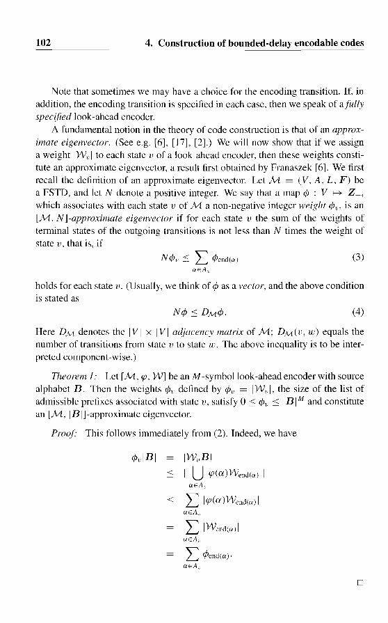
102 4. Construction of bounded-delay encodable codes

Note that sometimes we may have a choice for the encoding transition. If, inaddition, the encoding transition is specified in each case, then we speak of afully

specified look-ahead encoder.A fundamental notion in the theory of code construction is that of an approx­

imate eigenvector. (See e.g. [6], [17], [2].) We will now show that if we assigna weight IWuI to each state v of a look-ahead encoder, then these weights consti­tute an approximate eigenvector, a result first obtained by Franaszek [6]. We firstrecall the definition of an approximate eigenvector. Let }vl = (V. A, L, F) bea FSTD, and let N denote a positive integer. We say that a map cP : V f--+ Z+,which associates with each state v of M a non-negative integer weight cPu, is an[M, N]-approximate eigenvector if for each state v the sum of the weights ofterminal states of the outgoing transitions is not less than N times the weight ofstate v, that is, if

N cPu :s L cPend(OI)OIEA v

(3)

holds for each state v. (Usually, we think of cP as a vector, and the above conditionis stated as

(4)

Here DM denotes the IVI x IVI adjacency matrix of M; DM(V, w) equals thenumber of transitions from state v to state w. The above inequality is to be inter­preted component-wise.)

Theorem I: Let [M. <po W] be an M-symbollook-ahead encoder with sourcealphabet B. Then the weights cPu defined by cPu = IWul, the size of the list ofadmissible prefixes associated with state v, satisfy 0 :s cPu :s IB IM and constitutean [M, IBI]-approximate eigenvector.

pro(~r This follows immediately from (2). Indeed, we have

cPulBI IWuB[

< I U<p(a)Wend(OI) IOIEA v

< L 1<p(a)Wend(Q') IOIEA v

L IWend(01) IOIEA v

L cPend(OI)'OIEA v

o

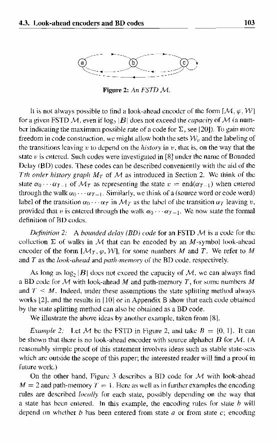
4.3. Look-ahead encoders and BD codes 103

ba _-c=.)D----- ---Figure 2: An FSTD M.

It is not always possible to find a look-ahead encoder of the form [M, cp, W]for a given FSTD M, even if log2 IB I does not exceed the capacity of M (a num­ber indicating the maximum possible rate of a code for L:, see [20]). To gain morefreedom in code construction, we might allow both the sets W v and the labeling ofthe transitions leaving v to depend on the history in v, that is, on the way that thestate v is entered. Such codes were investigated in [8] under the name of BoundedDelay (BD) codes. These codes can be described conveniently with the aid of theTth order history graph MT of M as introduced in Section 2. We think of thestate au ... aT-I of MT as representing the state v = end(aT-I) when enteredthrough the walk au· .. aT~ I. Similarly, we think of a (source word or code word)label of the transition au' .. aT in M T as the label of the transition aT leaving v,provided that v is entered through the walk au ... aT -I. We now state the formaldefinition of BD codes.

Definition 2: A bounded delay (BD) code for an FSTD M is a code for thecollection L: of walks in M that can be encoded by an M -symbol look-aheadencoder of the form [M T , cp, W], for some numbers M and T. We refer to Mand T as the look-ahead and path-memory of the BD code, respectively.

As long as log2 1BI does not exceed the capacity of M, we can always finda BD code for M with look-ahead M and path-memory T, for some numbers Mand T :s M. Indeed, under these assumptions the state splitting method alwaysworks [2], and the results in [10] or in Appendix B show that each code obtainedby the state splitting method can also be obtained as a BD code.

We illustrate the above ideas by another example, taken from [8].

Example 2: Let M be the FSTD in Figure 2, and take B = {O, I}. It canbe shown that there is no look-ahead encoder with source alphabet B for M. (Areasonably simple proof of this statement involves ideas such as stable state-setswhich are outside the scope of this paper; the interested reader will find a proof infuture work.)

On the other hand, Figure 3 describes a BD code for M with look-aheadM = 2 and path-memory T = 1. Here as well as in further examples the encodingrules are described locally for each state, possibly depending on the way thata state has been entered. In this example, the encoding rules for state b willdepend on whether b has been entered from state a or from state c; encoding

104 4. Construction of bounded-delay encodable codes

<' [11]11] ab [111 a ab [11

1 c [0,10]

[11]o a [11]

<' [0,101 c~ c [0,101[0] cb

o c [0,1C1] cb [0]

Figure 3: A two-symbol look-ahead encoder for M*.

rules for other states will not depend on history. (Hence we have T = I.) Thenotation in Figure 3 is (hopefully) evident; the lists of admissible prefixes W a =

{11}, We = {OO, 01, 1O}, Wah = {1O, II}, and Weh = {OO, Ol} are represented inthis Figure by the short-hand notation [11], [0, IOJ, [I], and [0], respectively.

To obtain this code, we first transform M into a FSTD M* by splitting state b"backwards" into a state ab (which can only be entered from state a) and a state cb(which can only be entered from state c). Then we can construct the look-aheadencoder for M* as shown in Figure 3. (Code construction for this example isdiscussed again in Example 3 in the next section.)

Each transition in M* has a unique "parent" transition in M. Hence an en­coding path in M* produces a unique encoding path in M. On the other hand, thepresent transition in the encoding path in M, together with the previous transition,uniquely determines the present transition in M*; in other words, the code has apath-decoding Ivindow of size two. Note that a look-ahead encoder for M 1 (asrequired by the formal definition of a BD code in Definition 2) can be constructedimmediately from Figure 3. D

Decoding a BD code for M requires the reconstruction of the transitions of theencoding path in MT, each of which is made up of T + I consecutive transitionsin M. In other words, the code for ~ has a path-decoding window of size T + 1;decoding of a particular transition in M also requires knowledge of the T previoustransitions. For future reference, we state this observation separately as a theorem.

Theorem 2: A BD code for M as in Definition 2 has a path-decoding windowof size T + 1, where T denotes the path-memory of the code.

We stress again the fact that from a BD code for M we can obtain a codefor the constrained system £ generated by M, provided that the labeling mapL of M is of finite type. (Indeed, to encode a given source sequence, read offthe code word labels of the walk produced by the BD code.) A code for I:- ofthis type will be referred to as a BD code for £. Note that if the labeling L isof finite type, then the walk in M can be "sliding-block" reconstructed from the

4.4. Local encoder structures and BD partitions 105

code word sequence generated by the walk, so that the corresponding BD codefor £.- is sliding-block decodable.

We see that essentially, a BD code for M is obtained by subdividing statesof M according to their history, that is, by "backwards state splitting". In contrast,the ACH state splitting algorithm subdivides states according to their future. (In[4] these fundamental operations are termed in-splitting and out-splitting, respec­tively.) The construction methods that we shall propose later can be consideredas a mixture of these two methods, where states are subdivided according to boththeir history and future.

BD codes were introduced by Franaszek in [8], where they were termed "sta­tionary" BD codes. The more general "periodic" BD codes in that paper are, inour terminology, BD codes for higher-order power graphs (see Section 2) of M.

4.4 Local encoder structures and BD partitions

A major drawback of BD codes is that their construction, as described in a se­quence of papers by Franaszek [6]-[9], involves a complicated process of parti­tioning state-trees and can be difficult. In this section we describe a much simplerconstruction method. Its main feature is that it partitions the (difficult) globalcode construction problem into a number of independent (relatively easy) localconstruction problems, one for each state of the FSTD. The local problem in aparticular state requires the construction of a local encoder structure in that state,and involves only the weights assigned to that state and its successors. As we willshow, it is fairly easy to construct a BD code once a local encoder structure isobtained in each state.

Contrary to Franaszek's method, our method does not always succeed. Indeed,there may be states for which no local encoder structure exists. This can happenif the weights of the successors to that state do not "fit together". Fortunately, thisproblem can always be solved by using state splitting to break down the weightsof (some of) the successors into smaller weights, as will be explained in the nextsection.

The motivation for our method is the following. Let us consider a BD code[MT, W, <p] for a FSTD M, with source alphabet B and path-memory T (seeDefinition 2). Recall that a BD code associates with each state v of M variouslists of admissible prefixes, one for each particular history in v (represented bywalks of length T ending in v). Sometimes such a BD code is very regular, inthe sense that, for each state v, these lists can all be obtained from one special listof words (representing the common "structure" of these lists) by a process thatwill be called relabeling. (Then, as we will see, a local encoder structure can be

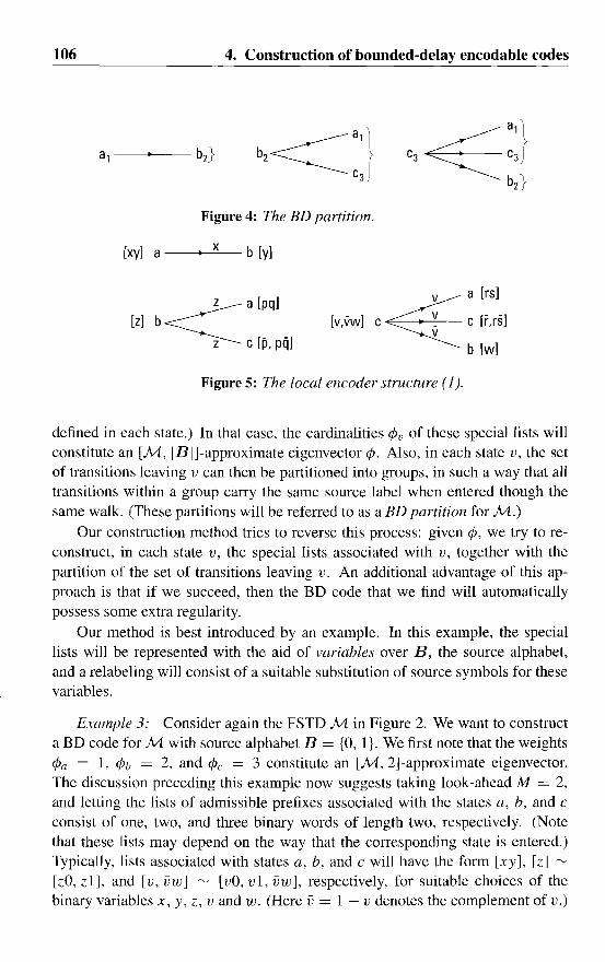
106 4. Construction of bounded-delay encodable codes

Figure 4: The ED partition.

[xv] a ----.-,-,-x_ b [y]

~a[pq]

[Z]b~

Z c [ii, pq]

v a [rs]

[v,'wl c4 c [f,rs]

b [w]

Figure 5: The local encoder structure (1).

defined in each state.) In that case, the cardinalities <Pv of these special lists willconstitute an [M, IB I]-approximate eigenvector <p. Also, in each state v, the setof transitions leaving v can then be partitioned into groups, in such a way that alltransitions within a group carry the same source label when entered though thesame walk. (These partitions will be referred to as a ED partition for M.)

Our construction method tries to reverse this process: given <p, we try to re­construct, in each state v, the special lists associated with v, together with thepartition of the set of transitions leaving v. An additional advantage of this ap­proach is that if we succeed, then the BD code that we find will automaticallypossess some extra regularity.

Our method is best introduced by an example. In this example, the speciallists will be represented with the aid of variables over B, the source alphabet,and a relabeling will consist of a suitable substitution of source symbols for thesevariables.

Example 3: Consider again the FSTD M in Figure 2. We want to constructa BD code for M with source alphabet B = {O, I}. We first note that the weights<Pa = I, <Pb = 2, and <Pc = 3 constitute an [M, 2]-approximate eigenvector.The discussion preceding this example now suggests taking look-ahead M = 2,and letting the lists of admissible prefixes associated with the states a, b, and cconsist of one, two, and three binary words of length two, respectively. (Notethat these lists may depend on the way that the corresponding state is entered.)Typically, lists associated with states a, b, and c will have the form [xy], [z] '"'-'[zO, zl], and [v, vw] ~ [vO, vi, vw], respectively, for suitable choices of thebinary variables x, y, z, v and w. (Here v = I - v denotes the complement of v.)

4.4. Local encoder structures and BD partitions

[DO] ° [O]~ a [00]a--+--b~ 1 a [00]

° c~ c [1,01] 1 [00][1,0~ ~a

[~]~c [1,01]

Figure 6: Encoder construction.

107

Note that we have opted for the simplest possible structure [z] of lists associatedwith state b.

The first and most important step in the construction is to find in each statea partition of the outgoing transitions into groups that will always receive equalsource labels. In Figure 4 we give a local description of the FSTD M, and, ineach of the states, a partition of the outgoing transitions. The indices to the statenames in this figure indicate the weight of the states, a convention that will beadopted throughout this paper. Note that these partitions cOlTespond to the formof the "local encoding rules" in Figure 5. (Here, x, y, z, p, q, rand s representbinary variables.) In fact, the choice of these partitions is immediate once we havefixed the structures ofthe lists of admissible prefixes as we did. Let us explain thisfor state c. (A similar argument applies to the other two states.) Suppose that. fora certain history in state c, the list of admissible prefixes in c is [v, vw]. Then thelists associated with the terminal states of transitions leaving c and labeled withsource symbol v together must contain each binary word of length two. (There areno further restrictions on upcoming sequences of source symbols that begin with asymbol v). Hence the sum of the weights of these terminal states must be at leastfour. Similarly, the sum of the weights of terminal states of transitions leaving cand labeled with source symbol vmust be at least two. Consequently, the partitionmust be the one as indicated in Figure 4. A description of local encoding rules asin Figure 5 will be termed the local encoder structure.

Observe that all lists in Figure 5 associated with the same state are equal upto renaming variables. Therefore we might try to build an encoder based on thelocal encoding rules in Figure 5, substituting ~ppropriate source symbols for thevariables according to need, that is, depending on how a state is entered. (Remarkthat no substitution of symbols for the variables in Figure 5 gives a look-aheadencoder; in particular, no encoder exists for which the list in state b is independentof history.) This idea is further illustrated by Figure 6, where we show how theencoder is gradually developed, starting with list [00] for state a. (Read this figurefrom left to right.) Proceeding in this way we again obtain the BD code describedearlier in Example 2. D

108 4. Construction of bounded-delay encodable codes

o1

2

o1

o

Figure 7: The parsing tree of U.

1

1 2

o

Figure 8: A labeling ofthe parsing tree of u.

After this example, the reader will surely wonder whether a valid local encoderstructure as in Figure 5 can always be transformed into an encoder with finite path­memory. The answer turns out to be yes, even with path-memory T :=: M. Beforewe show this, we will present a more formal description of our method and thenotions involved.

For the BD code derived in Example 3, the various lists of admissible prefixesassociated with a given state may depend on history, but they all have a simi­lar structure. The structure of a set of words is described by its parsing tree, a(directed, rooted) tree obtained by arranging these words into a tree structure.

Example 4: The parsing tree associated with the set of words

U = {OO, 01, lO, 21, 22}

is the tree at the left in Figure 7. Indeed, if the arcs of this tree are labeled asshown at the right in Figure 7, then U is the set of words obtained by reading offthe labels of paths from the root to a leaf in this tree. D

Definition 3: Let U and W be two sets of words, all of a fixed length M. Wesay that W is a relabeling of U if the arcs of the parsing tree of U can be labeledin such a way that each word in W is the label sequence of some path from theroot to a leaf in this tree.

Example 5: Let U be the set of words in Example 4, and let

W = {lO, II, 12,OO}.

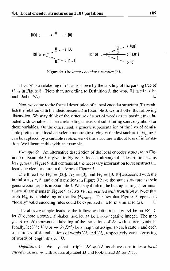
4.4. Local encoder structures and BD partitions

[00] a-----+----=-0_ b [0]

109

o a [00][O]b~

~C[l,01]

o a [00]

[0,101c~ c [1,011

b [0]

Figure 9: The local encoder structure (2).

Then W is a relabeling of U, as is shown by the labeling of the parsing tree ofU as in Figure 8. (Note that, according to Definition 3, the word 01 need not beincluded in W.) D

Now we come to the formal description of a local encoder structure. To estab­lish the relation with the ideas presented in Example 3, we first offer the followingdiscussion. We may think of the structure of a set of words as its parsing tree, la­beled with variables. Then a relabeling consists of substituting source symbols forthese variables. On the other hand, a generic representation of the lists of admis­sible prefixes and local encoder structure (involving variables) such as in Figure 5can be replaced by a suitable realization of this structure without loss of informa­tion. We illustrate this with an example.

Example 6: An alternative description of the local encoder structure in Fig­ure 5 of Example 3 is given in Figure 9. Indeed, although this description seemsless general, Figure 9 still contains all the necessary information to reconstruct thelocal encoder structure in the form of Figure 5.

The three lists W a = [00], W" = [OJ, and We = [0, 10] associated with theinitial states a, b, and c of transitions in Figure 9 have the same structure as theirgeneric counterparts in Example 3. We may think ofthe lists appearing at terminalstates of transitions in Figure 9 as lists Wa associated with transition a. Note thateach W a is a relabeling of the list Wend(a). The fact that Figure 9 represents"locally" valid encoding rules could be expressed in a form similar to (2). D

The above example leads to the following definition. Let M be an FSTD,let B denote a source alphabet, and let M be a non-negative integer. The mapcp : A 1--+ B represents a labeling of the transitions of M with source symbols.Finally, let W : V U A 1--+ P(B M ) be a map that assigns to each state v and eachtransition a of M collections of words W v and W a , respectively, each consistingof words of length Mover B.

Definition 4: We say that a triple [M, cp, W] as above constitutes a localencoder structure with source alphabet B and look-ahead M for M if

110 4. Construction of bounded-delay encodable codes

i) at least one set W v is non-empty,ii) for each transition ex, the set Wa is a relabeling of Wend(a), andiii) for each state v, we have

WvB <; U cp(ex)Wa.aEA v

(5)

The above definition should be compared with Definition 1 in the previoussection. In particular, we see that if W a is equal to Wend(a) for each transition ex,then the local encoder structure is in fact a look-ahead encoder for M.

We claimed earlier that a local encoder structure for M can be used to con­struct a BD code for M. Our next theorem, which is one of the main results inthis paper, states this in a precise way and, moreover, provides an upper boundon the path-memory of the resulting BD code. The proof, which can be found inAppendix A is not difficult but involves many details. Therefore, the reader isadvised to skip the proof on first reading. (The technique used in the proof to con­struct the desired BD code can and will be replaced by more "ad hoc" techniquesin our examples.) In Appendix B, we indicate another way to obtain an encoder.

Theorem 3: Suppose that the triple [M, cp, W] constitutes a local encoderstructure with look-ahead M for M. Then we can construct an M-symbollook­ahead BD code for M, with the same source alphabet and with path-memoryat most T, that is, a BD code for M with a path decoding window of size atmost T + 1. Here T .::: M denotes the smallest number with the property thateach of the sets Wa can be obtained from the parsing tree associated with W v byrelabeling up to depth T only.

In general we can obtain many different BD codes from a given local encoderstructure. But of course we want to find one with smallest possible path-memorysince such a code will have the smallest possible decoding window. Fortunatelythis optimizing problem is easy and can be dealt with by hand, or otherwise bycomputer. (A good illustration is provided by Example 9 in the next section.)

The construction method suggested by Definition 4 and Theorem 3 will betoo general for our purposes. The problem is that we would like to construct thelocal encoder structure for each state separately, but unfortunately a particularchoice for the set W v in one state may affect the construction in other states. Notehowever that once the sets W v are chosen, the requirements in Definition 4 can beverified locally for each state.

Therefore, with the sole exception of Example 3 in Section 8, we will restrictourselves to the case where (the structure of) the sets W v in Definition 4 is deter­mined by the desired look-ahead M and a given approximate eigenvector cp, in thefollowing way. For a given weight CPv, we let W v consist of the CPv smallest words

4.4. Local encoder structures and BD partitions 111

of length Mover B, with respect to the lexicographical order. Here, we assumethat the symbols of B have been ordered in some way. Then a word x = x I ... X M

is smaller than a word Y = YI'" YM if XI" 'Xk-l = YI'" Yk-I and Xk < Yk

holds for some k, 1 :s k :s M. Intuitively, these sets have the "simplest" structureamong all sets of words of a given size. (This structure does not depend on thechosen ordering on B.) So, in Example 3 we choose Wb = {OO, Ol} (with struc­ture [z]) and not {OO, ll} (with structure [ZX, zy]), given that cPb = 2 and M = 2.For completeness' sake we note that restricting the structure of the sets W v as heredoes not limit the scope of our method if it is combined with state splitting, as wewill do later. For example, if in Example 3 a set Wb = {OO, II} were required,then we would first split state b into two states bO and bl , each of weight one. Thenboth WbO = {OO} and Wbl = {ll} have the required structure. Concerning thesize of the sets IWv I, in Theorem 4, we will show that the weights IWvl obtainedfrom a local encoder structure necessarily constitute an approximate eigenvector.

Now we turn our attention to the remaining local construction problem. Sosuppose that we are given a source alphabet B, a number M, and an [M, IBI]­approximate eigenvector cP, and suppose furthermore that we have chosen thesets W v as explained above. By construction, there is a number nv such thatthe set W v contains all words of length M that begin with one of the first n v

symbols from B, and possibly some of the words that begin with the (n v + 1)thsymbol, and hence these symbols will appear as a label on the outgoing transitionsin state v. Consequently, to complete the construction, the most important taskthat remains is to find a suitable partition of (a subset of) the outgoing transitionsinto nv (or nv +1) groups of transitions that will receive the same source label. Onthe other hand, it is fairly easy to determine whether a given partition can indeedbe completed to a local encoder structure for state v, in the sense that appropriatelabels can be assigned to the groups such that the resulting labeling cp and suitablerelabelings W a of the sets Wend(a) satisfy ii) and iii) in Definition 4.

Definition 5: If a given partition of (a subset of) the outgoing transitions instate v can be completed to a local encoder structure in v in the above sense, thenthis partition is called a BD partition for state v, relative to M and cP.

It is very important to realize that whether a given partition of the outgoingtransitions in a state v is indeed a BD partition for v depends only on the numberM and the weights of v and its successors. Consequently, the above approach re­duces the (global) code construction problem to a local one in each state, involvingonly the amount of look-ahead and the weights of that state and its successors.

Example 7: Consider again Example 3. The partitions given in Figure 4 areindeed BD partitions relative to M = 2 and weights cPa = 1, cPb = 2, and cPc = 3,

112 4. Construction of bounded-delay encodable codes

as witnessed by the local encoder structure given in Figure 9. Note that eachlist WI' in this figure consists of the ¢v smallest words of length 2 over B asrequired. 0

We may even remove the dependence on M: without loss of generality wemay take M to be the smallest number for which ¢v .:s IB IM holds for all states v.

This can be seen as follows. First note that if we have a local encoder structure instate v with look-ahead M, then we can immediately obtain one with look-aheadM + I by defining new lists W~ and W~ and a new labeling <p' by W:! = OWl"W~ = <p (a) We;, and <p' (a) = 0, for all transitions a leaving v, where 0 denotesthe smallest source symbol in B. Conversely, if ¢v .:s IBIM - 1 holds for allstates v, then, since by assumption each WI' consists of the ¢v smallest wordsof length M, each WI' will be of the form OW~, and hence each We; will be ofthe form <p'(a)W~, for some source symbol <p'(a). It is then easily checked that[M, W', <p'] again constitutes a local encoder structure, but now with look-aheadM - 1. (Further details are left to the reader.)

Our next theorem states some necessary conditions that a BD partition (or,more generally, the partition induced by the labeling <p of a local encoder struc­ture) has to satisfy. The first part of this theorem generalizes Theorem 1 andexplains our restriction imposed on the cardinality of the sets WI'.

So let [M, <p, W] denotes a local encoder structure with look-ahead M andsource alphabet B. We denote by AI' = UhEBAe the partition of the set of out­going transitions AI' in state v induced by <p; here Ae consists of the transitions a

in AI! for which <p(a) = b. (Note that some of the parts may be empty.) Let ¢v

denote the number of words IWv I contained in WI'.

Theorem 4: With the above notation, ¢ is an [M, N]-approximate eigen­vector, where N = IB I denotes the cardinality of B. Moreover, for each state v

of M we have

(6)

In particular. if WI' consists of the ¢v smallest words in B M , then the number ¢t:of words in WI' beginning with symbol b satisfies

¢e .:s LN- 1 L ¢end(e;)J.e;EAe

(7)

The proof of this theorem (which is similar to the proof of Theorem 1) togetherwith a discussion of a nice corollary can be found in Appendix A.

Our methods may be summarized as follows.

4.5. A general construction method 113

Construction method for BD codes:Given an FSTD M and an [M, IBI]-approximate eigenvector cP, let M be thesmallest number such that cPu :::: 1B 1M holds for each state v of M. Furthermore,for each state v, let Wu consist of the cPu smallest words of length Mover B.Then,for each state v separately, try to find a BD partition of the set of transitionsleaving state v, and construct the corresponding local encoder structure in thisstate. This last step requires that we find, for each transition a leaving v, a suitablerelabeling of the set of words Wend(a) and a suitable source symbol <p(a), wherethe partition induced by <p is precisely the BD partition. If a local encoder structureis found in each state, then Theorem 3 guarantees the existence of a BD code withlook-ahead M and path-memory at most M.

Given an FSTD M and an [M, IBI]-approximate eigenvector cP, how difficultis it to determine whether a BD partition w.r.t. cP exists? This problem is discussedin detail in Appendix A. It turns out that the worst-case complexity of this problemis (at least) exponential in dmax , the maximum number of transitions leaving astate. The reader should not worry too much about this exponential behaviour.Indeed, note that even the complexity of finding a partition of Au satisfying thenecessary condition (7) in Theorem 4 is already exponential in IA u I. Nevertheless,the reader will surely agree that as long as 1 Au 1 is not too big, this last problem caneasily be handled. (Here we see the reason why the desired rate p / q of the codeshould have small q.) For small M, say M :::: 3, finding a BD partition turns out tobe comparable in difficulty to this last problem, and, according to our experience,is easy for values of dmax at least up to 10. This conclusion is supported by theexamples in Section 8.

4.5 A general construction method

In this section we supplement the methods in the previous section to obtain ageneral construction method for sliding-block decodable codes for a constrainedsystem of finite type. The many examples that we will give, both in this sectionand in Section 4.7, show that the method works very well and enables the designby hand of "good" codes, that is, codes with small decoding windows and simpleencoders, even for rather complicated constraints. Some of the reasons why thismethod works so well are discussed in Appendix B.

To understand our method, the reader should have some working knowledgeof state splitting. If this is not the case, we suggest consulting Appendix Bor [19]. In what follows, we assume that the constraints are represented by agiven FSTD M of finite type. We also assume that we are given an [M, N]­approximate eigenvector cP, where N denotes the desired size of the source alpha-

114 4. Construction of bounded-delay encodable codes

bet B. (Possible necessary preparations are discussed in Section 2. A simple algo­rithm to compute such an approximate eigenvector has been given by Franaszek,and can be found for example in [2].)

In the previous section we showed that a BD code for M can be obtainedonce a BD partition is found in each state. However, there may be some statesfor which no BD partition exists. For example, let N = 2, and suppose that Mcontains a state v with precisely two successor states a and b. If M = 2 andif v, a, and b all have weight 3, then no BD partition in state v exists. (Notealso that increasing the value of the allowed look-ahead M does not solve theproblem.) However, if one of the successors of v could be split into a state ofweight 1 and another one of weight 2, then after this state splitting operation a BDpartition for v would exist. (The reader should verify this! Precisely this situationwill also be discussed in Example 8 below.) This simple example suggests theuse of state splitting operations to transform the weighted FSTD M until ourlocal construction method applies, and leads to the following three-stage codeconstruction scheme.

In stage one, we transform the pair M, </J into a new FSTD M' and a new[M', N]-approximate eigenvector </J' by state splitting. Here, we try to minimizethe number K of rounds of state splitting needed to make the second stage suc­ceed. (Note that each additional round of state splitting will increase the size ofthe decoding window by one symbol).

In the second stage, we construct a local encoder structure for M' from a BDpartition with respect to </J' in each state of M'.

In the third and final stage, we use this local encoder structure for M' toconstruct a BD code for M'; in fact, one that provides a code for the constrainedsystem £ generated by M with smallest possible decoding window.

The third stage of the above scheme is easy and could be handled by computerif desired. (This will be further illustrated by our examples.) The main difficultyof our approach is to "coordinate" the first two stages. Unfortunately, it is noteasy to formulate strict rules on how to choose between various possible statesplitting steps. However, we will see from our examples that for many practicalapplications the above guideline is sufficient. Since this scheme obviously extendsthe ACH-algorithm [2], we are guaranteed to find some code.

A nice feature of the above approach is that code-construction methods such asthe ACH-algorithm [2], the BD-method of Franaszek [8], ideas described in [17],variable-length codes, and variable-length state splitting as in [3], [11] can all bethought of as special cases of the above scheme. In particular, the ideas from [17]become clearer when considered in this light. We will illustrate this with an ex­ample.

4.5. A general construction method 115

Figure 10: The local description ofM.

21 -----+--- 32}

22 04}

Figure 11: The BD partitions in the remaining states.

Example 8: Let M be the five-state FSTD with local description as in Fig­ure 10. (This is the same FSTD as the one considered in Example 2 from [17].)Also shown in this figure are the weights (indicated as a subscript to the state num­bers) that constitute an [M, 2]-approximate eigenvector, and a BD partition in allstates except state 1, for which no such partition exists. (Here, we take M = 2.)Therefore, in stage one we must split a successor of state 1, hence we must splitstate 2, and the only possibility is to split state 2 into states 21 and 22, of weight 1and 2, respectively. Let M' denote the FSTD thus obtained. In Figure 11 weshow the result of the state split, as weB as a BD partition for states 1,21 and 22.Since we have now found a BD partition in each state of M, we can constructa BD code for M with source alphabet B = {a, I} of size two. Stage three istrivial here, since it is evident that we can even obtain a two-symbol look-aheadencoder based on M', as shown in Figure 12. The resulting code for M has a(path-)decoding window of size 1 (actual transition) + 1 (the split) = 2. [J

We remark that the other examples in [17] can be handled in a similar way.Up to now, we have illustrated the theory with "artificial" examples only. Our

next example changes that situation; we now construct a code which has consid­erable practical applications.

Example 9: In this example, we will construct a rate 1/2 (2, 7)-code witha decoding window of size four code words or eight bits. (Recall that a (d, k)­

constrained sequence is a binary sequence in which each run of zeros has a length

116 4. Construction of bounded-delay encodable codes

a 0 [-] a 1 [0,10]

[-I 04 1 [0,101 [0,101142, [11]

4 [11] 22 [0]

<1[0,101[11] 21 3 [1]

[1] 3 [0] 220

0 [- ]1 4 [11]

[11] 4 3 [1]

Figure 12: A two-symbol look-ahead encoder based on MI.

of at least d and at most k. Here we consider the case where d = 2 and k = 7.)In [2], a rate 1/2 code for this constraint is constructed to illustrate the ACH statesplitting algorithm. We will do likewise here.

The FSTD commonly used to generate (2, 7)-constrained sequences has eightstates numbered 0, I, ... ,7, where the numbering is such that a sequence gen­erated by a walk ending in state vends in precisely v zeros. Since we aimfor a rate 1/2 code for this constraint, we let M be the second power of thisFSTD (so M is labeled with two-bit code words), and we take the source alpha­bet B = {O, 1}. The local structure of M is given in Figure 13. The smallest[M, 2]-approximate eigenvector involves weights between 1 and 4, so we chooseM = 2. (The weights of the states are indicated in Figure 13 as subscripts to thestate numbers.)

For all states except states 2 and 3 a BD partition can be found, as indicatedin Figure 13. (For state 6, we may choose either one of the indicated parts.)

Since no BD partition for states 2 and 3 exists, some state splitting is required.Inspection of Figure 13 shows that we have to split either both states 4 and 5, orstate 1. We choose to split state 1, into a state 11 with weight one and single suc­cessor state 0, and state h with weight two and single successor state 3. (Splittingstate 1 seems appropriate in view of the successor situation at state 7. However,the other choice also leads to a code with an eight-bit decoding window. Thiscode, whose derivation we leave to the reader, is only slightly less regular thanthe code obtained below. Yet another approach would be to split all of states 1,4, and 5. This would of course complicate stages two and three since more BDpartitions have to be considered, but even by hand these complications could stillbe dealt with easily.)

After splitting state 1, a BD partition can be found in each state. (In fact, inmost states we need to consider several BD partitions. In what follows we willsee how to handle this freedom of choice.) So we can now move to stage three of

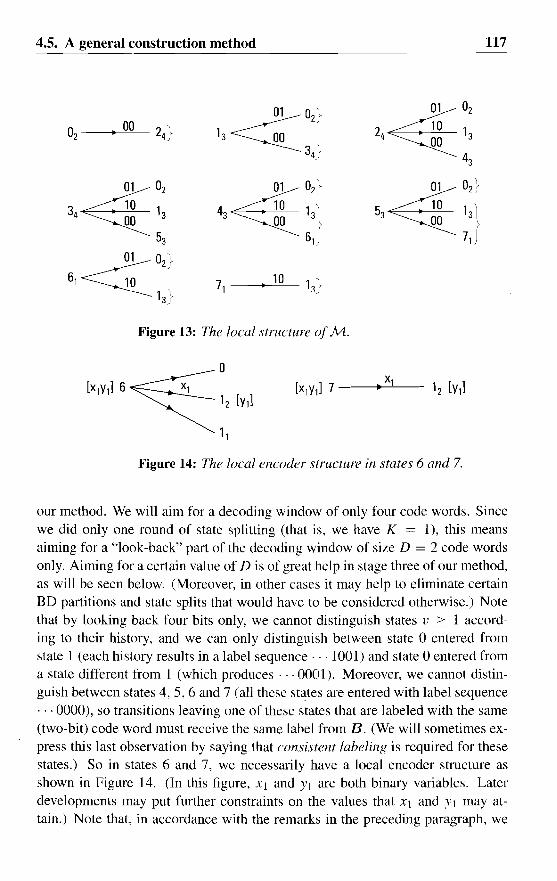
4.5. A general construction method 117

401 °2}

4 10 1 'I3 00 3\

61}

401 02

2 10 14 00 3

43

401 02}

5 10 1}3 00 3

71

Figure 13: The local structure ofM.

o[X1Y1]6~~ 12 [y,]

11

[X1Y,] 7 __....._X.!....1-- 12 [Y1]

Figure 14: The local encoder structure in states 6 and 7.

our method. We will aim for a decoding window of only four code words. Sincewe did only one round of state splitting (that is, we have K = 1), this meansaiming for a "look-back" part of the decoding window of size D = 2 code wordsonly. Aiming for a certain value of D is of great help in stage three of our method,as will be seen below. (Moreover, in other cases it may help to eliminate certainBD partitions and state splits that would have to be considered otherwise.) Notethat by looking back four bits only, we cannot distinguish states v ::=: 1 accord­ing to their history, and we can only distinguish between state a entered fromstate 1 (each history results in a label sequence· .. 1001) and state aentered froma state different from 1 (which produces· .. 0001). Moreover, we cannot distin­guish between states 4,5,6 and 7 (all these states are entered with label sequence... 0000), so transitions leaving one of these states that are labeled with the same(two-bit) code word must receive the same label from B. (We will sometimes ex­press this last observation by saying that consistent labeling is required for thesestates.) So in states 6 and 7, we necessarily have a local encoder structure asshown in Figure 14. (In this figure, Xl and YI are both binary variables. Laterdevelopments may put further constraints on the values that Xl and .vI may at­tain.) Note that, in accordance with the remarks in the preceding paragraph, we

118 4. Construction of bounded-delay encodable codes

41 12 [yd

Xl 0 [Y2]

[x"x2xd5 X2 1 [XIY2]

X2 7 [xlY,]

a)

41

12

X2 0

[x2,x,Yd 5 X2 1,

c) X2 7

[Yd

[X2]

[X1Y2]

[xlyd

Figure 15: The possible encoder structures in state 5.

41 12[yd

Zl 0 [x2]

[-]3 Z2 11 [X1Y2]

Z2 5 [X2'X1Y,]

[Y,] 12_----+---'-Y-'---l- 3 [-I

_----+---'-Y"---2_ 2 [_]

Figure 16: The encoder structures in the remaining states.

have assigned the same prefix list [Yl] to both state h entered from state 7 andstate h entered from state 6 (each history of state h produces 001 0, irrespectiveof the particular state from which 12 is entered). Also, we have labeled both thetransitions from state 6 to 12 and from state 7 to 12 with the same source symbolXl, since both these transitions have code word label 10 and states 6 and 7 cannotbe distinguished (both states are invariably entered with 0000). We will implic­itly use a similar reasoning when we develop the local encoder structures in theremaining states.

There are three possible BD partitions in state 5, which lead to the three pos­sible local encoder structures in Figure 15. Here, in all three cases, we requirethat {Xl. X2} = {YI, Y2} = to, I}. To each of the three local encoder structuresin state 5, there corresponds a similar local encoder structure in state 4. There isa unique BD partition in state 3, in which one part consists of the transitions tostates 12 and 0, and the other part consists of the transitions to states 5 and II.

The local encoder structures a) and b) in Figure 15 in state 5 assign sets ofwords to states II and 5 that cannot be combined. Therefore in state 5 we musttake the local encoder structure c) in Figure 15. This choice detetwines the local

4.5. A general construction method

[1) 0 2 [-)~12[0]

[0'1) 110

0 [1] o 0 [1]

[0) 120

3 [-)[-) 2 ~ 11 [01)

4 [1,00)

~12[O] 4 12[0]o 0 [1) 1 0 [1)

[-) 3 ~ 11 [01) [1,00) 4 ~ 11 [01)

5 [1,00) 6 [00)4 12[01

0

10016~111 0 [1)

[1,00) 5 ~ 11 [01] 12 [0)

7 [00) [00) 7~ 12 [0)

11

Figure 17: A two-symbol look-ahead encode!:

119

encoder structure in the remaining states as indicated in Figure 16. (The localencoder structure for state 4 is similar to the one for state 3.) Remark that thelocal encoder structure in state 3 imposes the constraint that XI = YI. Finally, if wetake for example XI = 0 = ZI, then we find the two-symbol look-ahead encoderin Figure 17, which indeed constitutes a rate 1/2 (2, 7)-code with a decodingwindow of size four symbols or eight bits, We will show in Example II that thiscode has a six-state encoder graph. (The code derived in [2] has the same decodingwindow size but requires a seven-state encoder.) Our code is actually equivalentto one of the codes that can be obtained from the uniquely decipherable prefix listin Table II of [2], and is among the best codes known for this constraint. Observethat our method produces this code almost automatically. 0

We end this section with some remarks on the problem of how to choose thestate splitting steps in the first stage. One approach (which is consistent withour examples) would be to choose only state splitting steps that do not destroyBD partitions (or "partial" BD partitions) constructed earlier. Let us call suchstate splits nice. First note that we certainly obtain a ae-consistent state split withrespect to the approximate eigenvector 4> (see [19] or Appendix B) in a state if welet the successors of one of the two offsprings consist of the union of one or more

120 4. Construction of bounded-delay encodable codes

of the parts of the partial BD partition in that state. Of course, splitting a state insuch a way does not destroy the partial BD partition in that state.

We mention here without proof that an ae-consistent state split with respect tocP of the above type in a state v of weight cPv .:::: N M is nice if, moreover, one ofthe two offsprings of v has a weight v satisfying 1 .:::: v .:::: N k or v == cPv mod N l ,

where N k is the highest power of N dividing cPv and N l - J < v .:::: N'. (The reasonis that under these conditions the set of the v smallest words of length Mover Bhas the same structure as the set consisting of the v largest words in W v , the setof the cP" smallest words of length Mover B.)

Unfortunately, this approach works often, but not always; it is possible to con­struct examples where no nice state split exists. Nevertheless, a useful heuristic isto use nice state splits whenever this is possible.

We believe that the method in its present form is best implemented interac­tively; the user chooses state splitting steps and BD partitions from alternativesproposed by the program, but leaves further calculations as well as the optimizingin stage three to the computer.

In the next section we discuss how to design finite-state encoders for this typeof code. Further applications of our code-construction method will be given inSection 4.7.

4.6 Finite-state encoders from look-ahead encoders

We now investigate how to obtain an encoder graph, and hence an ordinary finite­state encoder. from a given look-ahead encoder. Since a BD code is a speciallook-ahead encoder, the construction below also applies to BD codes.

So let [M, cp, W] be an M-symbollook-ahead encoder, with source alpha­bet B. We will think of an internal state of the encoder as being determined by apair (v, b), consisting of a state v of M together with a word b = bl ... bM in W v

obtained by looking ahead at upcoming source symbols. Then, to encode b l , theencoder first looks ahead one further symbol to see b = bM + j, then picks a tran­sition a leaving v for which cp(a) = bj and b' = b2 ··· bMb E Wend(a); as a resultthe encoder now moves to the internal state determined by (end(a), b'). We maythink ofthis internal transition as being labeled with source/transition label b/ a.

In what follows, we will find it convenient to think of the encoder as movingfrom a set of encoding alternatives to another such set. To this end, we associatewith each pair (v, b) the collection L",b consisting of all walks a = a, ... aM forwhich cp(a) = cp(ad" 'cp(aM) equals b. So Lv,b consists of all possible encod­ing paths starting in v that encode the word b. We will refer to these collection of

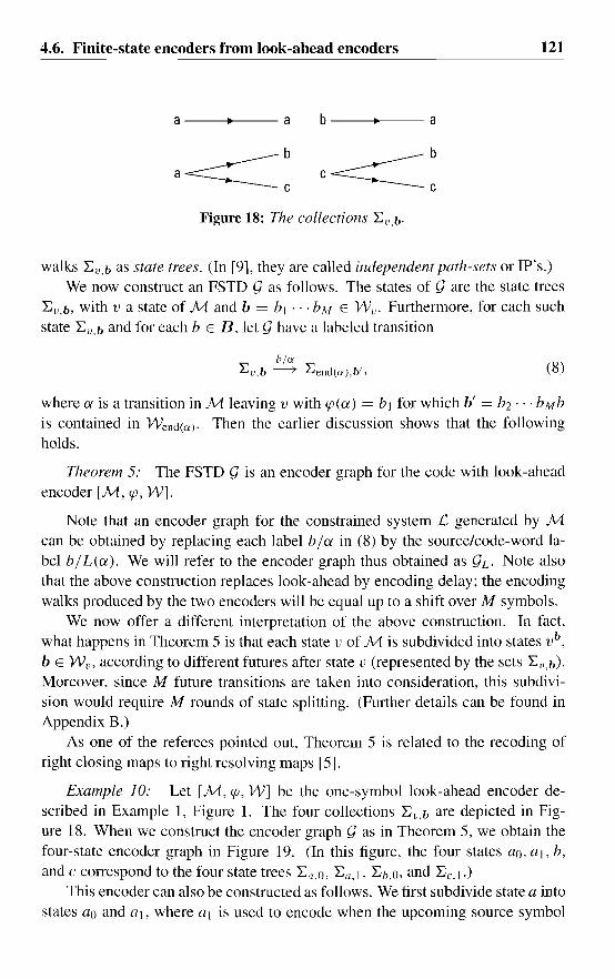
4.6. Finite-state encoders from look-ahead encoders 121

a--_---a b--_---a

Figure 18: The collections ~v,b.

walks ~v,b as state trees. (In [9], they are called independent path-sets or IP's.)We now construct an FSTD y as follows. The states of yare the state trees

~v,b, with v a state of M and b = b l ... bM E W v . Furthermore, for each suchstate ~v,b and for each b E B, let y have a labeled transition

b/a~v,b -----+ ~end(a),b" (8)

where a is a transition in M leaving v with cp(a) = bJ for which b' = b2'" bMbis contained in Wend(a). Then the earlier discussion shows that the followingholds.

Theorem 5: The FSTD y is an encoder graph for the code with look-aheadencoder [M, cp, W].

Note that an encoder graph for the constrained system £, generated by Mcan be obtained by replacing each label b j a in (8) by the source/code-word la­bel bjL(a). We will refer to the encoder graph thus obtained as YL. Note alsothat the above construction replaces look-ahead by encoding delay; the encodingwalks produced by the two encoders will be equal up to a shift over M symbols.

We now offer a different interpretation of the above construction. In fact,what happens in Theorem 5 is that each state v of M is subdivided into states vb,

bE W v , according to different futures after state v (represented by the sets ~v,b).

Moreover, since M future transitions are taken into consideration, this subdivi­sion would require M rounds of state splitting. (Further details can be found inAppendix B.)

As one of the referees pointed out, Theorem 5 is related to the recoding ofright closing maps to right resolving maps [5].

Example 10: Let [M, cp, W] be the one-symbol look-ahead encoder de­scribed in Example 1, Figure 1. The four collections ~I!.b are depicted in Fig­ure 18. When we construct the encoder graph y as in Theorem 5, we obtain thefour-state encoder graph in Figure 19. (In this figure, the four states ao, aJ, b,

and c conespond to the four state trees ~a,O, ~a, 1, ~b,O, and ~c, I.)

This encoder can also be constructed as follows. We first subdivide state a intostates ao and aI, where al is used to encode when the upcoming source symbol

122 4. Construction of bounded-delay encodable codes

o 0.~-------{ b

oo

l----------{ C

Figure 19: Afinite-state encoder.

equals 1 (so al will have successors b and c), and ao is used otherwise (so ao willhave successors ao and al). As a result each of the states ao, ai, b, and c nowencodes precisely one source symbol, which appears on all transitions leaving thestate. Next, we shift back all source labels by one transition: the (common) sourcelabel on the transitions leaving a state is now assigned to all transitions enteringthat state. The result is the encoder graph presented in Figure 19. Note that thisconstruction is in fact the same as the construction in Theorem 5, and producesthe same encoder graph.

The codes produced by the encoders in Figure I and Figure 19 are indeedequal up to a shift over one symbol. For example, to encode the source se­quence 0110010 from state a the encoder in Figure 1 produces the encoding pathaacbaaba, and the encoder in Figure 19, starting in state ao, encodes the sourcesequence 110010 (the previous sequence with the first symbol dropped) into thecorresponding path aoalcbaOalb.

To fully appreciate our final remark, the reader should probably be somewhatfamiliar with state splitting. Observe that the encoder in Figure 19, being obtainedfrom the FSTD in Figure 1 by one round of state splitting, has a path-decodingwindow of size two; beside the present transition in Figure 1, the decoder needs toknow (at least when this transition ends in a) one future transition to determine thecorresponding transition in Figure 1. However, the reader can easily verify thatknowledge of the future transition only is sufficient for decoding! Consequently,the "effective" path-decoding window size is only one instead of two. (This isof course evident in view of the equivalence of the two codes.) Part of this papermay be seen as an effort to profit from such "reduced window" phenomena in asystematic way. D

Both encoder graphs y and YL will have LVEV IWv I states, which can belarge. Fortunately, the number of states of YL can usually be reduced by statemerging (cf., Section 4.2). This operation applies for example when the outgoingtransitions in two states can be paired off in such a way that the two transitions

4.6. Finite-state encoders from look-ahead encoders

Table 1: The encoder.

source symbol inputpresent 0 1

state output next state output next state

A 10 E 10 FB 01 E 01 F

C 00 A 10 B

D 00 C 00 B

E 00 A 00 B

F 00 C 00 D

123

in each pair have the same source/code-word label and end in the same state. Ifthis is the case, then each source sequence will be encoded from both states bythe same code word sequence. Consequently, these states can be identified. thatis, merged into one state. This operation is applied repeatedly until no more statescan be identified. (In fact, this approach ensures that all states that can be mergedwill be identified eventually; since (h is deterministic w.r.t. the source/code-wordlabeling, it is reduced in this way to its Shannon cover, see e.g. [2] or [19].)

Example II: In this example, we consider the construction of an encodergraph for the (2, 7)-code obtained in Example 9. Only the main points are dis­cussed here, the details of the construction are left to the reader.

Since there are 21 distinct pairs (v, b) of states v and words bin W v , appli­cation of Theorem 5 leads to an encoder graph with 21 states. However, due tothe regularity of the code, the number of states can be reduced to six by merging.Indeed, the reader may verify that

i) States L:2,00, L:3,00. L:4,00. L:s,oo, L:6,00, and L:7,00 merge into one state A,ii) states L: 11 ,01. L:2,01, L:3,01, L:4, II. and L:s, 11 can be merged into one state B,iii) states L:2,]O, L:3,]O, L:4,IO, and L:s, 10 can be merged into one state C,iv) states L:2,11 and L:3,11 can be merged into one state D,v) states L:O,IO and L: 12,00 can be merged into one state E, andvi) states L:O,11 and L:1 2 ,01 can be merged into one state F.These merging operations lead to the six-state encoder with input/output relationsas in Table 1. D

In the remainder of this section we discuss a (partial) converse to Theorem 5.Our results will establish a further link with the work in [9], and will be used inAppendix B to investigate codes produced by the ACH state splitting algorithm.Suppose that, in each state v of an FSTD M, the set of walks of length M startingin v is pat1itioned into mutually disjoint collections L:v,i, i = 1, ... , n v , again

124 4. Construction of bounded-delay encodable codes

referred to as state trees. We write

ct~v,i -----+ ~w,j (9)

if a is a transition in M from v to w such that for each walk al ... aM in ~w,j, thewalk aal ... aM-I is contained in ~v,i' We construct a graph 9 with as "states"the state trees ~v,i, and with "transitions" of the form (9). Let B be a set of size Nand suppose that each state ~v,i of 9 has at least N successors. Then, in each state,we can label N transitions leaving that state with the N distinct symbols from B.So 9 now has labeled transitions

b/ct~v,i -----+ ~w,j, (10)

and looks like an encoder graph.Observe that walks in 9 generate walks in M, and, because the state trees

are disjoint, distinct right-infinite walks in 9 generate distinct right-infinite walksin M. So we conclude that 9 is the encoder graph of a code for M. Note that wemay obtain such a graph 9 from a BD code [M, cp, W] with path memory 0, asin Theorem 5.

What kind of code is generated by the encoder graph 9? We will show thatin fact such a code is a BD code, although not necessarily one with path memoryO. To state the precise result, we need some preparation. We define a (partial)labeling cp of the transitions in the Mth history graph MM of M (that is, ofthe walks of length M + I in M) as follows. Let cp(ao' .. aM) = b whenever

b/ctoao·· . aM-I E ~v,i, al ... aM E ~w,j, and ~v,i -----+ ~w,j holds for some iand j, where v = beg(ao) and w = end(ao). (Since the state trees are disjoint, iand j are determined uniquely.) Note that then cp(aofh ... f3M) = b holds for allwalks f31 ... f3M in ~w,j' Now, for each walk a = ao·· .aM-I in M (that is, foreach state a of M M), let the set Wn consist of all words bo ... bM-I for whichthere is a walk in 9 of the form

(11)

With these definitions of cp and W, we have the following result.

Theorem 6: The triple [MM, cp, W] constitutes an M-symbollook-aheadBD code for M with path memory (at most) M. This BD code is equal to thecode generated by 9 up to a shift over M symbols.

Proof' Let a = ao··· aM-I be a state in MM, let bo" . bM-I be a wordin Wn, and let b E B. To prove the first part of our theorem, we need to show thatthere is a transition in MM, with source label bo, from a to some other state ai,

4.7. Further examples

Table 2: The admissible words of length 5.

label word term. state parityinit. state

a 00000 (+5) -

b 00001 0 ec 00010 1 0

d 00100 2 ee 01000 3 0

f 01001 0 0

g 10000 4 eh 10010 1 e

Table 3: The approximate eigenvector.

125

say, such that the word bl ... bM-,b is contained in Wa,. This can be seen asfollows. By the definition of Wa , there is a walk as in (11) in g. Since each statein 9 has a leaving transition with source label b, there is a transition in 9 of the

f b/a I d fi " " f W h"orm ~vM.iM -----+ ~w •.i' Let Q = al ... aM-Ia. By e mtlOn 0 ai, t IS setcontains the word b l ... bM-Ib. Since necessarily Q E ~vo,io and Q' E ~vl"il' itfollows from the definition of cp that the transition ao ... aM-Ia in M M leavingstate Q has source label cp (ao ... a M-I a) = bo as required.

To prove the second part of our theorem, we reason as follows. Suppose that9 encodes a sequence {bn} of source symbols into a walk {an} in M. From thedefinition of cp we then conclude that cp(an ... an+M) = bn, that is, in the BDcode the source label bn is assigned to transition an+M (provided its history isan'" an+M-d. D

4.7 Further examples

In this section we use our construction method to derive three new codes, all with asmaller decoding window than the best codes known for the constraints involved.

4.7.1 A new rate-2lS (2, 18, 2)-constrained code

Our first example concerns the construction of a rate-2/5 (2, 18, 2)-constrainedcode with a decoding window size of 3 code words or 15 bits, and error propaga­tion of 5 bits.

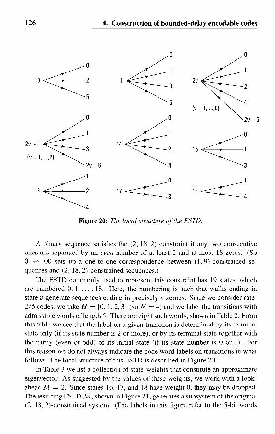
126 4. Construction of bounded-delay encodable codes

Figure 20: The local structure of the FSTD.

A binary sequence satisfies the (2, 18,2) constraint if any two consecutiveones are separated by an even number of at least 2 and at most 18 zeros. (Soo B 00 sets up a one-to-one correspondence between (l, 9)-constrained se­quences and (2, 18, 2)-constrained sequences.)

The FSTD commonly used to represent this constraint has 19 states, whichare numbered 0, 1, ... , 18. Here, the numbering is such that walks ending instate v generate sequences ending in precisely v zeroes. Since we consider rate­2/5 codes, we take B = {O, 1,2, 3} (so N = 4) and we label the transitions withadmissible words oflength 5. There are eight such words, shown in Table 2. Fromthis table we see that the label on a given transition is determined by its terminalstate only (if its state number is 2 or more), or by its terminal state together withthe parity (even or odd) of its initial state (if its state number is 0 or 1). Forthis reason we do not always indicate the code word labels on transitions in whatfollows. The local structure of this FSTD is described in Figure 20.

In Table 3 we list a collection of state-weights that constitute an approximateeigenvector. As suggested by the values of these weights, we work with a look­ahead M = 2. Since states 16, 17, and 18 have weight 0, they may be dropped.The resulting FSTD M, shown in Figure 21, generates a subsystem of the original(2, 18, 2)-constrained system. (The labels in this figure refer to the 5-bit words

4.7. Further examples 127

a~

07fc 1

1/3/59 : 39

6/8/1011

~07}'

C 19

11/13/154 e 39

°7bh 19

2/412

~-----o,........:::.d_ 212

9412

19

6/8/1011 ~---=---- 212}

Figure 21: The FSTD M.

in Table 2.) As usual, the weights of the states are represented as indices to thestate-number. We have also indicated a BD partition for those states that have one.(Unique only for state 0.)

We see that all states except 2, 4 and 1, 3, 5 have a BD partition. Some statesplitting on the successors of these states is needed, but as we will see, one roundwill do. So we will choose K = 1. A lot of freedom remains, though, both inthe choice of state splitting operations and in choosing the BD partitions. Onepossibility is to split all relevant successors of states 2, 4 and 1,3,5 (that is, states2,3,4, states 7, 9, and states 6, 8, 10), and then to use a computer to optimize instage three over all possible BD partitions. Although this would be feasible, wechoose a different approach.

Let us be ambitious and aim for D = 1, i.e., for a decoding window of threecode words only, an improvement of one code word compared to the best codeknown (see [19]). Once the present transition in M is known, we require one codeword look-ahead to determine the corresponding transition after state splitting(which is also sufficient since M is deterministic). The present code word, whennot equal to a = 00000, determines both the parity of the initial state of the present

128 4. Construction of bounded-delay encodable codes

~o[1,30,31,33] b ° [1,30,31,33]

[1,30,31,33] ~ a 5 [0,2,32] [0,1,3] 1 [0,2,32]

° 3 d 22 [0,1,3] 2 [0,1,3]

7/9ae [2]

° [1,30,31,33]

[0,2,32] 1 [0,2,32]

1,3,5 4 [1,2,3]3 [0,2,32]

6/8/1°7 [1,30,31,33] b ° [1,30,31,33]a

6/8/1°4 [2][1,2,3] 1 [0,2,32]

4

~o[1,30,31,33]

2 [0,1,3]

° 7/9ae [2]° c 1 [0,2,32]

[0] 7/9cf

[2] 7/9ae 2 e~3 [0,2,321 4 [1,2,3]

a 12/14 [1,30,31,33]0 [1,30,31,33]b

~o[1,30,31,33]

[0,2,32]

[1,30,31 ,33] ~ h 1[1,30,31,33] 1

[0,2,32] 12/14

6/8/107 3 d2 [0,1,3]

2 [0,1,3]4

[2]

6/8/10.~ ~O[1,30,31,33]

2 4 [1,2,3] °

a 11/13/15 [0][0] 0 c 1 [0,2,32]

11/13/15 e 3

Figure 22: The resulting code.

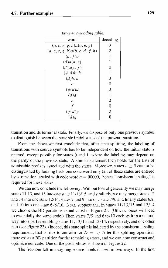
4.7. Further examples

Table 4: Decoding table.

129

word decoding(a,c,e,g,h)a(a,e,g) 3

(a, c, e, g, h)a(b, c, d, j, h) 2(b, f)a 1

(d)a(a, e) 1(d)a(c, f) 0(# d)b, h 1

(d)b, h 3C 0

(# d)d 3(d)d 1

e 2j 0

(# d)g 2(d)g 0

transition and its terminal state. Finally, we dispose of only one previous symbolto distinguish between the possible initial states of the present transition.

From the above we first conclude that, after state splitting, the labeling oftransitions with source symbols has to be independent on how the initial state isentered, except possibly for states 0 and 1, where the labeling may depend onthe parity of the previous state. A similar statement then holds for the lists ofadmissible prefixes associated with the states. Moreover, states v :::: 5 cannot bedistinguished by looking back one code word only (all of these states are enteredby a transition labeled with code word a = 00000), hence "consistent labeling" isrequired for these states.

We can now conclude the following. Without loss of generality we may mergestates 11,13, and 15 into one state 11/13/15, and similarly, we may merge states 12and 14 into one state 12/14, states 7 and 9 into one state 7/9, and finally states 6,8,and 10 into one state 6/8/10. Next, suppose that in states 11/13/15 and 12/14we choose the BD partitions as indicated in Figure 21. (Other choices will leadto essentially the same code.) Then states 7/9 and 6/8/10 each split in a naturalway into a part resembling states 11/13/15 and 12/14, respectively, and one otherpart (see Figure 22). (Indeed, this state split is indicated by the consistent labelingrequirement, that is, due to our aim for D = 1.) After this splitting operation,there exists a BD partition for the remaining states, and we can now construct andoptimize our code. One of the possibilities is shown in Figure 22.

The freedom left in assigning source labels is used in two ways. In the first

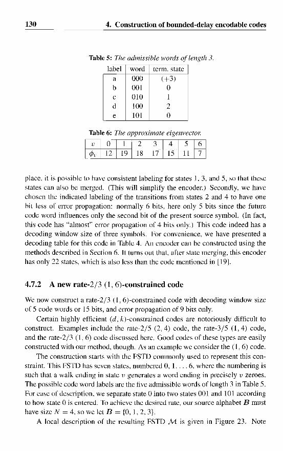
130 4. Construction of bounded-delay encodable codes

Table 5: The admissible words of length 3.

label word term. statea 000 (+3)b 001 0c 010 1d 100 2e 101 0

Table 6: The approximate eigenvector.

place, it is possible to have consistent labeling for states 1, 3, and 5, so that thesestates can also be merged. (This will simplify the encoder.) Secondly, we havechosen the indicated labeling of the transitions from states 2 and 4 to have onebit less of error propagation: normally 6 bits, here only 5 bits since the futurecode word influences only the second bit of the present source symbol. (In fact,this code has "almost" error propagation of 4 bits only.) This code indeed has adecoding window size of three symbols. For convenience, we have presented adecoding table for this code in Table 4. An encoder can be constructed using themethods described in Section 6. It turns out that, after state merging, this encoderhas only 22 states, which is also less than the code mentioned in [19].

4.7.2 A new rate-2/3 (1, 6)-constrained code

We now construct a rate-2/3 (1, 6)-constrained code with decoding window sizeof 5 code words or 15 bits, and error propagation of 9 bits only.

Certain highly efficient (d, k)-constrained codes are notoriously difficult toconstruct. Examples include the rate-2/5 (2,4) code, the rate-3/5 (1,4) code,and the rate-2/3 (1,6) code discussed here. Good codes of these types are easilyconstructed with our method, though. As an example we consider the (1 , 6) code.

The construction starts with the FSTD commonly used to represent this con­straint. This FSTD has seven states, numbered 0, 1, ... 6, where the numbering issuch that a walk ending in state v generates a word ending in precisely v zeroes.The possible code word labels are the five admissible words of length 3 in Table 5.For ease of description, we separate state 0 into two states 001 and 101 accordingto how state 0 is entered. To achieve the desired rate, our source alphabet B musthave size N = 4, so we let B = {O, 1,2, 3}.

A local description of the resulting FSTD M is given in Figure 23. Note

4.7. Further examples 131

415 511

001 12 001 12218

119 119

218 218

101 12 101 12

001 12 ~1"}119 511 218} ,

218 101d

218}101 12

67~10112}

67

001 12

317 415119

218

101 12

~317

101/00112~ 119

001 12

Figure 23: The local structure ofM.

that the code word label carried by a transition is determined by its end state.The smallest [M, 4]-approximate eigenvector 1> is listed in Table 6. In Figure 23these weights are indicated as usual as a subscript to the state number. We choosea look-ahead M = 2. As a consequence, the states 1, 2, and 3 (having a weightlarger than 16) have to be split into parts of weight at most 16. We choose thisvalue of M since a lot of state splitting is required anyway.

It is not difficult to verify from Table 6 and Figure 23 that in order to havea BD partition in each of the states, at least two rounds of state splitting are re­quired. Therefore, we choose K = 2. So our decoding window will contain twocode words of look-ahead, and since M is deterministic, this amount of look­ahead is also sufficient to determine the terminal state of a transition after tworounds of state splitting once the initial state in M is known. For states 5 and 6we choose the BD partition indicated in Figure 23. Other results (see [13]) nowsuggest splitting off from both states 1 and 2 a part of weight 16 (or parts withtotal weight 16). Moreover we have seen in our other examples that it is goodstrategy to split states in such a way that resulting offsprings can later be mergedwith other states. (This same heuristic is used in ordinary ACH to minimize thenumber of encoder states.) Observe that this aim is often automatically achievedwhen the choice of state splits is guided by a consistent labeling requirement.

The above discussion strongly suggests splitting states 4, 5, and 6 as indicated

132 4. Construction of bounded-delay encodable codes

52 24------ 18

Figure 24: First round of state-splitting.

001 12

Figure 25: Second round ofstate-splitting.

in Figure 24 and then combining the offsprings of weight 3 from these states withthe remaining successor states of states 1, 2, and 3 to form a part of weight 16,which can then be split off from these states in a second round of state splitting.(See Figure 25.) After these state splitting operations, we do indeed have a BDpartition in each state, as shown in Figure 26.

The BD partitions shown in Figure 26 are not unique: In the BD partition forstate 4r

, we may interchange states 251 and 252 , and for states 1/2/3 r• we may

also interchange states l4r and 4/5/6°. However there is obviously no advantagein not choosing consistent labeling between states 4r and 1/2/3r

, so essentiallythe only choice left is the above choice in state 4r

. It turns out that the best codeis indeed obtained by the choice indicated in Figure 26.

Now we have reached stage 3 of our method, where we optimize the code forthe smallest decoding window. Although our choice of state splitting operationshas been consistent with an aim for D = 1, that is, with an aim for a look-back of

4.7. Further examples 133

1r16 } 1r

16 }

3r16

l. t 16,

)J

001/1 01 1214r

3 14r3

362 25211

1/2/3r16

001 12001 12

}4/5/6°

1r16

t 16 } 2511

4r12 101 1214r

3

252 _____________ 4r12 }

1

14r

}001 12

3 512

51_____________ 4

,1 5/62 J

251_____________ 4

1 2/35/6

\

4/5/6°3 101d 514

1r16 }

5/624 t 16 }

Figure 26: The resulting FSTD with ED partitions.

only one code word, at this stage it turns out to be impossible to construct a BDcode achieving this aim. (This is easily verified as follows. Assign source symbolvariables to transitions, consistent between states originating from states v ::: 3.Then states 14,. and 252 necessarily have prefix lists that cannot be combined inthe BD partition for state 1/2/3", as would be required.) So we need a decodingwindow of at least five code words; two code words of look-back, the presentcode word, and two code words of look-ahead. A BD code with such a decodingwindow is shown in Figure 27. (The reader will have no difficulty to verify thattwo previous code words, the present code word, and two future code words areindeed sufficient to determine the actual transition followed in Figure 27.)

Note that the labeling is consistent between states v ::: 3 except for the labelsof transitions ending in state 2", which are either 3 (from states I /2/3" and 4")or 1 (from state 5/62

), and for the labels of transitions ending in state 101, which

134 4. Construction of bounded-delay encodable codes

c 1' [- ] 1' [- ]

3'c

[0,1,3] [- ]t [- ]

001 14r [20,22,23]a 14

, [20,22,23]

b362 [21]

[- ] 252 [21]

1/2/3'001 [0,1,3] 001 [0,1,3]

c 1' [- ]4/5/6° [01,02,03]

[1,2,3] 3' [- ]251 [00]

'10114

, [20,22,23]101 [1,2,3]

b362 [21]

001 [0,1,3][20,22,23]~ 4' [0,2,3]

c l' [- ] 14,

[0,2,3] t [- ] [00] ° a 51 [0]251~

4' 14, [20,22,23][2'1]~ 5/6

2[1]

252 [2'1] 2/35/62

001 [0,1,3][0]

251 [00]51 .0 C 1' [- ]

[01,02,03] [1 ]

4/5/6° .0 e 101 [1,2,3] 5/62 • 1 d t [- ]

Figure 27: The resulting code,

4.7. Further examples

a

135

o

o

d

Figure 28: The local structure ofM.

are either 1 (from state 1/2/3r) or 0 (from state 4/5/6°. Therefore an error in the

first code word in the decoding window can affect at most one bit of the originalsource symbol. So this code has an error propagation of 9 bits only (instead of theexpected 10 bits). Note however that the "span" of an error pattern can be 10 bits,so according to some definitions the error propagation would still be 10 bits.

Finally we note that, using the methods described in Section 6, we can find afinite-state encoder for this code having only 21 states.

4.7.3 A new rate-2/3 0, 9)-constrained code

As our final example, we construct a rate-2/3 (1, 9)-constrained code with decod­ing window size of 2 code words or 6 bits.

This example-which does not involve state splitting- is included to illus­trate the usefulness of the more general local encoder structures in Section 4 asa code-construction tool. Moreover, in this example we initially work without anapproximate eigenvector.

A classic method for constructing (d, k) codes is to forbid certain sequences ofwords in a suitable (d, (0) code, possibly in combination with certain substitutionrules. Our construction of a (l, 9) code is based on this idea; we will first constructa (I, (0) BD code, and then eliminate all encoding walks that generate the words000.000.000 or 000.000.001. (This is of course sufficient to obtain the desiredk-constraint, as the reader may easily verify.)

Our starting point to construct a rate 2/3 (l, (0) code is the FSTD M withlocal structure as in Figure 28. The code word labels are the five admissible wordsof length 3 given earlier in Table 5. Since we desire a rate of 2/3, we take N = 4,and we let B = {O, 1,2, 3}.

Our aim is to find a local encoder structure in each state of M, with an ad­ditional property. So we will assign prefix lists Wv and Wa and labels cp(a) tostates v and transitions a of M, where each W a will be a relabeling of Wend(a)

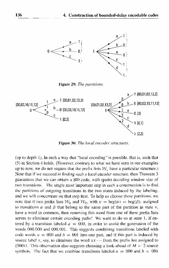
136 4. Construction of bounded-delay encodable codes

a

o

O}

d

Figure 29: The partitions.

~a 1 [00.ll1,02,13,2]

[00,03,10,11,12] 1o 0 ~ 0 [00,03,10,11,12]

1 [0,3]

a 1 [00,01 ,02,13,2]

o[00,03,10,11,12]

o[3]c

d1 [0,1]

1 [2,3]

Figure 30: The local encoder structures.

(up to depth 1), In such a way that "local encoding" is possible, that is, such that(5) in Section 4 holds. (However, contrary to what we have seen in our examplesup to now, we do not require that the prefix lists Wv have a particular structure.)Note that if we succeed in finding such a local encoder structure, then Theorem 3guarantees that we can obtain a BD code, with (path) decoding window size oftwo transitions. The single most important step in such a construction is to findthe partitions of outgoing transitions in the two states induced by the labeling,and we will concentrate on that step first. To help us choose these partitions, wenote that if two prefix lists W a and Wtl' with v = beg(a) = beg(j3), assignedto transitions a and j3 that belong to the same part of the partition in state v,have a word in common, then removing this word from one of these prefix listsserves to eliminate certain encoding paths! We want to do so at state 1, if en­tered by a transition labeled a = 000, in order to avoid the generation of thewords 000.000 and 000.001. This suggests combining transitions labeled withcode words a = 000 and b = 00 I into one part, and if this part is induced bysource label x, say, to eliminate the word xx ... from the prefix list assigned to(000) 1. This observation also suggests choosing a look-ahead of M = 2 sourcesymbols. The fact that we combine transitions labeled a = 000 and b = 001

4.7. Further examples 137

~a 1 [01,02,13,2)

[00,03,10,11,12)

(001) 0 ~ ~ 0 [00,03,10,11,12)

1 [0,3)

a

[3)~ 1 [13,2)

11011 0~ 0110,11,121

1 [0,3)

1 [01,02,13,2)

[01,02,13,2) o[00,03,10,11,12)

(000) 10[3)

d1 [0,3)

1 [1,2)

a 1 [01 ,02,13,2) a 1 [01,02,13,2)

[0,3) o[00,03,10,11,12) [1,2) o[00,03,10,11,12]

(010) 1 (100) 10[3) 0[3)

c

d1 [0,3)

d1 [0,3)

1 [1.2) 1 [1,2)

Figure 31: The resulting code.

imposes a constraint on the structure of the sets Wo and WI, which in turn elim­inates certain partitions. In fact, there is only one way to choose the partitionsnow, which is the one shown in Figure 29. These partitions suggest that we takeweights <Po = 5 and <PI = 8. A local encoder structure for M with all desiredproperties is shown in Figure 30.

From these local encoder structures we can construct the BD encoder in astraightforward manner. One of the possibilities is shown in Figure 31. Note thatcertain words are eliminated from prefix lists at the end of transitions in order tomake the encoder deterministic, and of course the word 00 is eliminated from theprefix lists associated with state (000) 1 in order to meet our k-constraint. Obvi­ously, our code has a decoding window size of two words: one word look-back todetermine the state in Figure 31, and then the present word to determine the actualtransition followed from that state. The code also satisfies the k = 9 constraint:if the word a = 000 is generated, then the encoder is in state (000) 1 and thusthe next two upcoming source symbols are not both zero, whence at most four

138 4. Construction of bounded-delay encodable codes

consecutive zero bits are generated next. It turns out that a finite-state encoder forthis code constructed as described in Section 6 has only 8 states.

We have some final remarks concerning this example. Of course, this codecould also have been constructed in a way similar to that used in other examples,statting from the third power of the FSTD commonly used to represent the (l, 9)­constraint. However, the code was actually found in the way described above(with the aim of meeting a k-constraint with smallest possible k), and since webelieve the method to be both interesting and potentially useful in similar situa­tions, we decided to present this construction method here. We conjecture that thevalue k = 9 is optimal, in the sense that no rate-2/3 (l, 8)-constrained code canhave a decoding window of only two code words.

4.8 Conclusions

We have presented a new technique to construct sliding-block decodable codeswith a small decoding window for constrained systems of finite type. Our meth­ods works very well when the maximum number of transitions from a state inthe FSTD-representation of the constraint is small. The power of this method isdemonstrated in several examples; these include the construction (by hand!) of arate-2/3 (d, k) = 0,6) code with a decoding window of only five code wordsor 15 bits.

The codes obtained by our method can also be constructed by means of theACH state splitting algorithm, provided that suitable choices are made for thestate splitting steps and the assignment of source symbols in the resulting en­coder graph. When constructed by state splitting, these codes will exhibit thereduced-window property: the effective decoding window will be (sometimesmuch) smaller than predicted from the number of rounds of state splitting usedin their construction. Indeed, our method could be incorporated into the ACHalgorithm to try and guide the choice of the state splitting operations.

Our approach is very suitable to construct codes by hand, possibly assistedby computer. Further research is needed to determine the best implementationby computer. Other topics for further research include the generalization of thismethod to the case where the constraints are of almost-finite type.

Acknowledgments

I would like to thank my colleagues J.H. van Lint, Sr. and K.A.S. Immink for theircomments on earlier versions of this paper, and L.M.G. Tolhuizen and C.P.M.Baggen for their help while preparing the final version.

4.9. Appendix A: additions to Section 4.4

4.9 Appendix A: additions to Section 4.4

In this appendix we collect some material connected to Section 4.

4.9.1 Proof of Theorem 3

139

The proof essentially formalizes the idea of encoder construction as in Figure 6of Example 3. In the proof, we will express the fact that a set of words is a rela­beling of another set of words with the aid of a relabeling map. Here, a relabelingmap is a map T : B M

f--+ B M with the property that if, for some number k, twowords x = Xl ... XM and Y = Yl ... YM from U agree in the first k symbols, thentheir images T (x) and T (y) also agree in the first k symbols.

It is easily seen that for U. W S; B M , W is a relabeling of U if and only if Wis the image of U under some relabeling map. (Indeed, if two words x and Y in Uare generated by paths in the parsing tree of U that agree in the first k arcs, thenafter relabeling the parsing tree, the same is true for their images T(X) and T(Y).)

In the proof, we construct for each walk rr in M a label <p (rr) in B, a set Wn

of words oflength M, and a relabeling map Tn such that the following holds.i) if two distinct walks rr and w agree in the last s transitions (or if they both endin the same state, if s = 0), then the words Tn (x) and Tev (x) agree in the lastM - T + s symbols (or are equal if s ~ T), for all words x = Xl ... X M.

ii) W n = Tn (Wend(n »),

iii) WnB S; UaEAend(Jr) <p(rra)Wna ,

We construct these objects inductively, for walks rr of length k, for k = 2,3, ....Remark that i)-ii) above hold for k = 1, and iii) for k = 0, according to theassumptions in the theorem. (By convention, a state is a walk of length 0.)

In what follows, we will need a few simple properties of relabeling maps or,more briefly, R-maps. If T : B M

f--+ B M is an R-map, then we denote by ithe map defined by i(XO··<tM) = r(xO···XM-I)XM. Also, if b,c E Baresuch that r maps all words beginning with the symbol b into words beginningwith symbol c, then we write rIb) to denote the map defined by i(bxl ... XM) =cr(lJ) (Xl' .. XM). The reader will have no difficulty verifying that both i and reb)

are again R-maps. Also, we observe that the composition ra of two R-maps rand a is again an R-map.

Now suppose that we have constructed objects <p(rr), W n , and rn as above forall walks of length less than k, and suppose furthermore that i)-iii) hold when­ever all objects involved in the statement are defined. Now let rr be a walk oflength k - 1. From the defining properties of a local encoder structure. we have

Wend(n)B S; U <p(a)Wa ,

aEAend(Jr)

140

hence by ii),

4. Construction of bounded-delay encodable codes

WnB = Tn (Wend(n) B) ~ U Tn (cp(a)Wa). (12)aEAendln)

For each transition a leaving end(JT), let us define the symbol cp(JTa) by

Tn (cp(a)Xl .. 'XN/) = cp(JTa)i~'I'(a))(XI" 'XN/), (13)

where i~'I'(a)) is the R-map defined from in as explained earlier. Next we note thatW a = ia(Wend(a». so if we define the R-map ina by ina = i~'I'(a»ia, then withthe aid of (13), we may express (12) as

Hence if we put

WnB ~ U cp(JTa)rna ( Wend(a»).Q'EAend(n)

(14)

W na = ina ( Wend(a)). (15)

then (14) shows that ii) and iii) also hold for the new objects. Let us now ver­ify that i) also holds. So suppose that the two distinct walks JT and w, each oflength less than k, agree in the last s transitions, and let a be a transition suchthat end(JT) = end(w) = beg(a). Let x = Xl ... XM be a word of length Mover B. By i), the words in (x) and i w (x) agree in the last M - T + s symbols.By definition of ina, we have that

(16)

and similarly,(17)

From the above expressions and from the definitions of Tn and To), it followsimmediately that ina (x) and iida (x) agree in the last M - T + s + 1 symbols, asrequired.

Now we shall use the objects constructed above to obtain the required BDcode. By i), the R-maps in (and hence also the sets of words W n ) constructedabove depend only on the last T transitions of JT. Consequently, if JT = JT] ... JTT

has length T and if JT! = JT2 ... JTT, then by iii) we have that

WnB ~ UaEAcndln) cp(JTa)Wna

= UaEAend(n) cp(JTa)Wn,a .

Therefore, the map cpo restricted to walks of length T + 1 in M (that is, to tran­sitions in M T), together with the sets of words W n for walks JT of length T (thatis, for states of M T), constitute an M -symbol look-ahead encoder for M T, thatis, a BD code for M with path memory T.

4.9. Appendix A: additions to Section 4.4

4.9.2 Proof of Theorem 4

141

Let us first observe that since Wa is a relabeling of Wend(a), we have

IWal ::: IWend(a)I = cPend(a). (18)

The fact that cP is an [M, IBI]-approximate eigenvector can now be shown in thesame way as in the proof of Theorem 1. But we can say more: if wt denotes thecollection of all words in WI' with prefix b, then we have

WtB ~ b U Wend(a)' (19)aEAt

So by combining (18) and (19), we obtain that

IW~IIBI ::: L cPend(a).aEAt

Moreover, we obviously have

hence we conclude that

IW~I ::: min ( LN- 1 Lh

cPend(a)J, N M-

1).

aEA"

Finally, since

cPV = IWvl = L IW~I.b

the theorem follows.

4.9.3 Some comments on Theorem 4

(20)

(21)

(22)

(23)

Although the necessary conditions for BD partitions in Theorem 4 are ratherstrong, they are not sufficient in general. However in the case where M = 1, agiven partition is a BD partition ifand only if these conditions hold, as the readercan easily verify. This observation has a nice consequence. A collection of parti­tions AI' = UbAe for each state of M induces in a natural way a similar collectionof partitions for the Mth power M M of M. Moreover, it is not hard to see that ifthe original partitions for M satisfy the conditions in Theorem 4 for some Nandfor look-ahead M, then the induced partitions for MM also satisfy these condi­tions, but now for alphabet size N M and look-ahead 1. From these observationswe may conclude that if for a given collection of partitions the conditions statedin Theorem 4 hold, then there exists a BD code for the Mth power MM of Mwith source alphabet B M , that is, a "periodic" BD code, a result first obtained byFranaszek [9].

142 4. Construction of bounded-delay encodable codes

4.9.4 The complexity problem for BD partitions

Let B = {a, ... , N - I} be a source alphabet and let M denote the word-length.For each integer n, °:s 11 :s N M, define W(M, n) to be the set of the n smallestwords of length Mover B. We investigate the complexity of the ED problem

BD(n, (ni liE I), M). Here nand ni, i E I, are integers with °:s n, ni :s N M,i E I, and the problem is to find a partition of I into parts h, b E B, such that

(24)

holds for suitable relabelings Wi of W(M, nd (or to verify that no such partitionexists). Note that by taking n = ¢v, I = A v, and no: = ¢end(o:) for a E Av weobtain the problem of finding a BD partition in state v.

Let us say that a subset J of I covers a set of words W ~ B M if W ~ Ui E]Wiholds· for suitable relabelings Wi of W(M, nd. Write n = qNM- 1+ r. °:s r <N M -I. From (24) it is easily seen that we need to find q + 1 mutually disjointsubsets J of I, q of which cover B M and one which covers W(M - 1, r)B.

How can we verify whether a given J ~ I covers W(M - 1, r)B? (To treatboth cases simultaneously, we also allow r = N M - 1 here.) Obviously, we shouldhave

r :s LN- 1 L lIiJ·iE]

(25)

(Cf. Theorem 4.) However, except when M = 1 this easily verified necessarycondition is not in general sufficient. We will show that, for M :::: 2, the ver­ification amounts to solving a BD problem, but now with word-length M - 1instead of M. To see this, write lli = qiNM-1 + ri, °:s ri < N M -

1, and note

that the set W(M, nd is the union of sets bBM - 1, b = 0, ... ,qi - I, and a fur­ther set qiW(M - 1, rd. Therefore, after a suitable relabeling the set Wi can bemade to cover any qi sets of the form bBM - 1, together with a set of the formbiW;, with W; a relabeling of W(M - 1, ri). Here bi can still be chosen arbitrar­ily in B. So together, the sets Wi, i E J, can be made to cover the sets bBM- 1

for°:s b < LiEJ qi, and it is easily seen that to verify whether the remaining partofW(M -1, r)B can also be covered we must solve BD(r - N M

-2 LiE] qi, (ri I

i E J), M - 1), a BD problem for word-length M - 1. (Note that possiblyr :s N M - 2 LiE] qi, in which case this last verification can be skipped.)

The above suggest the following recursive algorithm to solve the BD problem.

i) Find the minimal subsets of I that cover B M or W(M - 1, r)B. (In thisstage we may need to solve BD problems for smaller word-lengths.)

4.10. Appendix B: connection with the ACH algorithm 143

ii) Find disjoint subsets Jo, ... , Jq of I such that Jo covers W(M - 1, r)Band J1 •... , Jq each cover B M.

Even a partial solution in step ii) of this algorithm can be useful when the BDproblem has no solution, cf. Section 5.

Now what does this mean for the complexity problem for BD partitions? Notethat the worst-case complexity is (at least) exponential in dmax = maxVEV IAv I, themaximum number of transitions leaving a state. Moreover, the recursion depth ofthe algorithm is determined by M = maxVEV pogN <Pv l. The conclusion is thatour construction method for BD codes should be applied only when dmax and Mare not too big. Practical experience shows that the method can be applied easilyfor values of dmax at least up to 10 and M = 2 or 3. (Cf. Example 2 in Section 8.)

4.10 Appendix B: connection with the ACH algorithm

Here we will establish a connection between the ACH state splitting algorithmand our method, and thereby explain some of the reasons why our method is soeffective. We begin with a review of the ACH algorithm and its properties, as faras relevant here. For proofs of our claims and for further details we refer to [2] orthe excellent overview [19]. After this introduction to ACH, we will show that theBD method and the ACH algorithm are related by a time shift over M symbols,where M is the number of rounds of state splitting (see also [10]). Finally, weshow that our method is related to ACH by a time shift over K symbols, forsome K between 0 and M. Along the way we obtain a lower bound on M interms of the smallest possible maximal component of an approximate eigenvector,which may be of independent interest.

The ACH algorithm is a method to transform a given FSTD into an encodergraph. It is based on a certain type of transformation referred to as a round ofstatesplitting. Such a transformation produces from a given FSTD M a new FSTD M 'in the following way. For each state v of M, let the set A v of transitions leaving vbe partitioned into sets A~, i = l, ... , n v . We construct the FSTD M ' as follows.Each state v of M produces states vi, i = 1, ... , nv , in M ' , and each transition afrom state v to state w contained in A~ produces transitions

j = 1, ... , nw , in M ', all of which inherit their label from a. This constructionmakes precise the intuitive idea that each state v can be split into new states viaccording to different futures (represented by their possible successors). We referto states vi and transitions a i as to children of state v and transition a in M ' , and

144 4. Construction of bounded-delay encodable codes

to v and a as their parents in M, respectively. This notion of children and parentsextends to walks in M and M' in the obvious way.

The single most important property of this transformation is that all childrena'f3' in M' of a given walk af3 in M agree in transition a'. (Intuitively, we thinkof this property as a transition in M with givenfuture determining a unique transi­tion in M'.) Consequently, the parent/child relation in fact provides a one-to-onecorrespondence between bi-infinite walks in M and M' and, in pm1icular, Mand M' generate the same constrained sequences. In the terminology of Sec­tion 2, the labeling map L' that assigns to each transition of M' its parent in M(the ancestor map) is block-decodable, with window (0, 1).

We say that an FSTD M* is produced from the FSTD M by M rounds ofstate splitting if M* is the result of a sequence of transformations

where each intermediate transformation consists of a round of state splitting. Wemay extend the parent/child relation by transitivity to states and transitions in Mand M*. An easy induction argument then suffices to provide proof of the fol­lowing claims. Each state (transition) in M* has a unique parent state (transition)in M. Moreover, the parent/child relation provides a one-to-one correspondencebetween bi-infinite walks in M and M* and, in particular, M and M* generatethe same constrained sequences. Indeed, the ancestor map L * is block-decodable,with window (0, M): all children a5 ... a~ in M* of a given walk ao . .. aM in Magree in transition a5. We denote this transition by <I>(ao ... aM) and refer to it asthe transition in M* determined by the transition ao in M with future al ... aM.

The ACH state splitting algorithm in fact transforms a pair (M, ¢), where ¢ isan [M, N]-approximate eigenvector, and does so by what is called ae-consistentrounds of state splitting. (Here N is a positive integer representing the desiredcode rate.) We say that a round of state splitting that transforms Minto M' asexplained earlier is ae-consistent (with respect to the approximate eigenvector ¢)if, for each state v of M, the weight ¢v associated with v can be distributed overits children vi in M', in such a way that the resulting assignments of weights tothe states of M' now constitutes an [M', N]-approximate eigenvector. Moreover,to exclude various degenerate cases we require that at least one state v' of M' hasbeen assigned a non-zero weight smaller than the weight of its parent state in M.As a consequence of this last requirement there will be more non-zero weightsin M' than in M. It is not hard to see that a collection of partitions A~ provides aae-consistent round of state splitting precisely when

¢v ::s I)N- l L ¢end(O')J.

O'EA~

4.10. Appendix B: connection with the ACH algorithm 145

(Compare this requirement with the necessary condition for the existence of alocal encoder structure in Theorem 4.)

The main result in [2] applies to an in-educible FSTD M and states that ifthe non-zero weights in ¢ are not constant, then some ae-consistent split withrespect to ¢ can always be found. Consequently, after a finite number of trans­formations, the pair M, ¢ gets transformed into a pair M*, ¢* for which ¢* isan [M*, N]-approximate eigenvector with constant non-zero weights. Eliminat­ing zero-weight states from M* if necessary, we may assume that ¢* is constant,and then the definition of an approximate eigenvector reveals that, necessarily, atleast N transitions leave each state in M *. Consequently, by eliminating (if nec­essary) some states and transitions from M*, we may obtain an FSTD N that isan encoder graph for M (that is. precisely N transitions leave each state of N).In what follows, we assume that the transitions of N are labeled with source sym­bols from a source alphabet B of size N. in such a way that for each state of Nthe N transitions leaving this state all have distinct labels.

Let us now consider the decoder for the code produced by the encoder }if. Thecrucial observation is that the code has a path-decoding window of size M + I.Indeed, let the decoding function <p be defined as follows. For a walk ao ... aM

in M, let <p(ao' .. aM) denote the source label of the (unique) transition a* =<I>(ao ... aM) in M* determined by transition ao with future aj ... aM, providedthat a* is also present in N (¢ is left undefined otherwise). We will suppose thatthe labeling of M is ofjinite type (see Section 2), with memory m and anticipa­tion a, say. Consequently, from an encoded sequence f = {f,1} we may recovereach transition in the walk a = {an} in M generating this sequence by observ­ing m + I + a consecutive symbols from f. Finally, we can recover the originalsource sequence used to encode f = {f,,} from a = {an} through the decodingfunction <p, which essentially "reads off' source labels of successive transitionsa~ = <I>(an ... an+M) contained in the walk in N that generated f = Un}.

We now investigate the connection between the ACH algorithm and our me­thod. We will first use the encoder graph N to construct a collection of state treesin M, and then we will apply Theorem 6 to construct a BD code equivalent to theACH code up to a time shift over M symbols. For a state v* in N with parentstate v in M let b u* be the collection of parents in M of walks of length M in Nwith initial state v*. Observe that each b u* is non-empty, all walks in b u* haveinitial state v, and two sets b u* and b w * are disjoint for distinct states v* and w*in N. (Indeed, if ao ... aM is a walk in M with beg(aj) = v, then all children ofaj ... aM start from the terminal state v* of <I>(ao ... aM) in M*, and this state v*necessarily is a child of v.) Next, we write

(26)

146 4. Construction of bounded-delay encodable codes

if there is a transition a* from v* to w* in N with parent a and source label bin B.

Let the graph Q have as states the sets I;I'* and transitions as in (26). For eachwalk a of length M in M, let Wn consist of all words bo' .. bM - 1 that are asource labeling of some walk a* in N with parent a.

Theorem 7: The triple [MM, cp, W], where W is as defined above and wherecp is the decoder function, constitutes an M -symbol look-ahead BD code with pathmemory (at most) M. This code is equivalent to the original ACH code by a timeshift over M symbols.

Proof Since N is an encoder graph, each state I;v* in Q has N successors.Moreover, it is fairly obvious that Q and N generate the same code for M. Nowthe theorem is a direct consequence of Theorem 6. (It is easily verified that cp

and W as defined here coincide with those used in Theorem 6.) 0

The shifting mechanism referred to in the above theorem functions in the fol­lowing way. If cp(ao ... aM) = b, then in the ACH code the label b is assigned totransition ao with future al ... aM, while in the BD code the label b is assignedto transition aM with history ao ... aM-I.

Corollary 8: [10] A code constructed by the ACH algorithm (an ACH code)by M rounds of state splitting is equal to an M -symbol look-ahead BD code, upto a shift over M symbols.

Conversely, each BD code can be produced by the ACH algorithm, with anappropriate choice of approximate eigenvector and state splitting steps, and for anappropriate labeling with source symbols of the resulting encoder graph. More­over, given a local encoder structure with look-ahead M, an ordinary finite-stateencoder can be constructed directly by only M rounds of state-splitting.

Detailed proof of these statements, involving induction on the amount ofJook­ahead M in combination with a relabeling technique, is given in Appendix C.For completeness' sake, we sketch a proof of these statements here, using thenotation from Theorem 4. The idea is to split each state v into states vb, forb E B, according to the partitions Ae. (Theorem 4 shows that this splitting isae-consistent with respect to ¢.) Assign to state vb the set of words W2 ... W M forwhich bW2 ... W MEW!', and define the list of words associated with transitionsin a similar way. Also, a transition ending in state we is assigned label c. In thisway, we obtain a local encoder structure with look-ahead M - I, by one round ofstate splitting. Continue this procedure until the look-ahead equals zero.

From the above correspondence between ACH codes and BD codes we maydraw an interesting conclusion. Let ev denote the maximum value of IWn lover allwalks a oflength M ending in v. It is an easy exercise to show from Theorem 1

4.10. Appendix B: connection with the ACH algorithm 147

that e is an [M, N]-approximate eigenvector. Since obviously all components ofe have a value of at most N M, we obtain the following result. (This result alsofollows from Theorem 5 in [18].)

Theorem 9: If the ACH algorithm produces an encoder graph for M by Mrounds of state splitting, then N M :::':: L, where L denotes the smallest integer forwhich we can find an [M, N]-approximate eigenvector with all its components ofsize less than or equal to L.

We now come to the main observation of this section. It turns out that, fre­quently, the splitting steps in the ACH algorithm and the labeling with sourcesymbols of the resulting encoder graph N can be chosen in such a way that Nhas what we will call the reduced window property: There is a number T < Msuch that the function cp(ao' .. aM) depends only on aM-T ... aM, or in otherwords, only the T + 1 rightmost transitions in the (path-) decoding window arerequired for decoding. Consequently, the corresponding BD code has in fact path­memory T instead of M!

The reason why this can happen so frequently is more difficult to explain. Infact, elsewhere we will show that, given an FSTD M of finite type, the ACH algo­rithm is capable (with a suitable choice of approximate eigenvector) to construct,up to equivalence by a time shift, all sliding-block decodable codes that possess afinite-state encoder with finite encoding delay and a finite-type code word label­ing. (The same result has recently be obtained in quite a different way by Ashleyand Marcus [4].) If the required shift referred to above is larger than the "look­back part" of the decoding window of the given code, then the correspondingACH code will have the reduced window property.

Although there may exist a sequence of splitting steps such that the resultingencoder graph N, when suitably labeled with source symbols, has the reducedwindow property, it is not at all evident how to recognize suitable splitting stepsso as to work towards this property. (Some information concerning this problemcan be found in [13].) At first it would seem that code construction through theBD method only replaces this problem by another one of comparable difficulty.Fortunately, we may (at least partly) overcome these problems by mixing the BDmethod and the state splitting approach. Indeed, let us consider what happensif we stop state splitting after K rounds, for some number K between 0 and T.Let M' denote the resulting FSTD after these K rounds. (Observe that now atransition in M as well as K future transitions are needed to determine the corre­sponding transition in M'.)

We can then construct (essentially) the same code as in Theorem 7, but nowas an (M - K)-symbollook-ahead BD code for M'. The decoding function cp'

148 4. Construction of bounded-delay encodable codes

for MM-K is now defined as follows. If ab' .. a~_K is a walk in .lvt', then

where b is the source label of the transition aoin N determined by this walk(and undefined otherwise). Consequently, whenever ao ... aM is a walk in M forwhich as) ... a~_K is a child of ao ... aM-K in M', we have

Using this relation between cp and cp', it is easily shown that cp' (ab ... a~_K)depends in fact only on the last T - K + 1 transitions a~_T ... a~_K' (Indeed,suppose that the two walks ab' .. a~_K and fJb· .. fJ~-K in M' agree in the lastT - K + 1 transitions. Now if a~K+l ... a~ is a walk that extends both thesewalks, then the parent walks ao ... aM and fJo ... fJM of these extensions agree inthe last T + I transitions, whence

which proves our claim.)So we may conclude that the original ACH code is identical (up to a time

shift over M - K symbols) to a BD code for M' with look-ahead M - K andpath-memory T - K. In particular, for K = T we obtain a BD code with path­memory 0, that is, an (M - T)-symbol look-ahead assignment for M'. If wehave some luck, then the structure of the look-ahead assignments WVI associatedwith the states v' of M' is such that the methods in Section 4 apply. (Otherwisemore splitting steps would be required.) If we have still more luck, then evenfewer than T rounds of state splitting will do; this occurs if all sets Wal ...a l

M-T+! M-K

that correspond to walks a~_T+l ... a~_K ending in the same state have thesame structure. (See Section 4.) Our examples provide ample evidence that thisapproach is indeed a profitable one, requiring often only a few rounds of statesplitting to obtain good codes.

4.11 Appendix C: BD codes from ACH

Here, we begin by showing that each M -symbol look-ahead encoder or local en­coder structure [M, cp, W] can in fact be obtained from the pair (M, ¢) by ae­consistent state-splitting, where ¢v = IWvl, for all states v. (Later we discussthe case of general BD codes.) We first do this for a look-ahead encoder, then weindicate how to adapt the proof in the case of a local encoder structure.

1494.11. Appendix C: BD codes from ACH-----------------

In both cases, we transform the pair (M, cp) into a pair (M', cp') by ae­consistent state-splitting and the encoder [M, cp, W] into an encoder [M', cp', W']for a code, equivalent to the original code up to a shift, in the following way. Toobtain M', we partition each set Av of transitions leaving state v into sets Ae,for b E B, where Ae consists of all transitions a leaving v for which the sourcelabel cp(a) = b. So each state v splits into states vb, for all b E B, and eachtransition a, from v to w, say, produces transitions a C

, for all C E B, where a C isa transition from vb to w C

, with b = cp(a), which inherits its label L'(aC) = L(a)

froma.Also, in both cases we define the sets W' b as the collection of all words

vb2 · .. bM for which the word bb2 ... bM is contained in W v , and we let l' b =vIW:,b I· It is not difficult to check that l' is an approximate eigenvector for M'.(Altematively, we can invoke Theorem 4.)

In the case of a look-ahead encoder, we define cp'(aC) = c. We now claim

that [M', cp', W'] constitutes an (M - l)-symbollook-ahead encoder. Indeed,this follows immediately from the definition of a look-ahead encoder, togetherwith the observation that W v = UbEBW:,b holds for each state v. Moreover, it isan easy matter to check that encodings produced by this encoder are the same asthose produced by the original encoder, up to a shift by one symbol.

In the case of a local encoder structure, we have to adapt the definition of cp',and to define the sets W~" for transitions a' in M'. We proceed as follows. Recallthat we require the existence of a relabeling map (or R-map) T" : Wende,,) f--+

W" for each transition a of M (see Appendix A proof of Theorem 3). By thedefinition of an R-map, all words in Wende,,) that begin with a fixed source symbolc E B are mapped to words in W" that all begin with the same source symbol c',say. We slightly abuse notation and denote this source symbol c' by T" (c).

Now let W~c denote the collection of all words C2" . CM for which the wordr,,(c)c2' .. CM is the image under T" of a word in Wende,,) that begins with thesymbol c. Moreover, we let T~c : W~nd(")C f--+ W~c denote the map on W~nd(")C

"induced" by Ta . It is easily checked that the maps T~c are again R-maps.Finally, we define the source symbol labeling cp' of transitions in M ' by letting

cp'(a C) = T,,(C). Now, using the definition of a local look-ahead encoder and

the additional observation that W a = UcEBW~c holds for each a, it is a simplematter to check that [M', cp', W'] constitutes an (M - I)-symbol look-ahead localencoder structure. As before, there occurs a shift by one symbol.

The proof of our claims now follows by induction on M. Indeed, the aboveprocedure is repeated until the amount of look-ahead M is reduced to zero, inwhich case the resulting look-ahead encoder or local encoder structure in factrepresents an encoder for the original code, up to a shift by M symbols.

Now, we consider the case of an M-symbollook-ahead BD code [M T • cp, W]

150 References

based on the Tth order history graph M T of M. As shown above, an encoder foran equivalent code up to a shift over M symbols can be obtained from (MT, ¢),

where ¢CXO"CXT-l = IWCXO"'CXT_11 for all paths 0'0'" O'T-I in M, by M rounds ofae-consistent state-splitting. Therefore, in order to show that an equivalent en­coder can be obtained from M by ae-consistent state-splitting, it is sufficient toshow that the pair (M T, ¢) can be obtained through ae-consistent state-splittingfrom a pair (M, ¢(O)), for some approximate eigenvector ¢(O) for M. This canalways be achieved as follows. First, we consider the pair (M [T], ¢ ), where M [T]

denotes the Tth order edge graph of M, which is the same graph as MT, exceptthat a "transition" 0'0'" O'T now canies label L(O'o) instead of label L(O'T. (A"state" 0'0'" O'T-I is now best considered as the state v = beg(O'o) with "fu­ture" 0'0'" O'T-I.) Note that M T and M[T] generate the same sequences, butshifted over T symbolds. It is now fairly evident that the pair (M[T], ¢) can beobtained from T rounds of ae-consistent state-splitting from the pair (M, ¢(O)).

The intermediate pairs (M[k1, ¢(k)) occuring in the process are composed fromthe kth order edge graph M[k] and an approximate eigenvector ¢(k) for this edgegraph. Here, ¢~~~"CXk-l = Z=* ¢end(Jr), where the summation ranges over all pathsJr = 0'0' .. O'k-IJrk ... JrT-I starting in state v.

We note that under certain conditions ae-consistent state-splitting starting with(M, ¢) is also possible. This occurs for example when for each path 0'0 ... O'T -I,

the size of the set of words WCXO"'CXT_I only depends on the terminal state of thepath. In that case, the ae-consistent state-splitting process to obtain an encoderfor [MT. cp, W] from the pair (MT, ¢) can be made to conespond to a similarprocess starting with (M, ¢). We leave further details concerning this specialcase to the reader.

Ifwe combine the above results, we indeed find an ae-consistent state-splittingprocedure to obtain an encoder for our BD code [MT, cp, W].

References

[1] RL. Adler, RK. Brayton, M. Hassner, and B.P. Kitchens, "A rate-2/3 0,6)RLL code", IBM Techn. Disci. Bul., vol. 27, no. 8, Jan. 1985.

[2J RL. Adler, D. Coppersmith, and M. Hassner, "Algorithms for sliding blockcodes. An application of symbolic dynamics to information theory", IEEETrans. Inform. Theory, vol. IT-29, no. 1, pp. 5-22, Jan. 1983.

[3J RL. Adler, J. Friedman, B. Kitchens, and B.H. Marcus, "State splitting forvariable-length graphs", IEEE Trans. Inform. Theory, vol. IT-32, no. 1, pp.108-113, Jan. 1986.

References 151

[4] J. Ashley and B.H. Marcus, "Canonical encoders for sliding block deco­ders", Siam J. Disc. Math., vol. 8, no. 4, pp. 555-605, Nov. 1995.

[5] M. Boyle, B. Kitchens, and B.H. Marcus, "A note on minimal covers forsofie systems", Proc. AMS, vol. 95, no. 3, pp. 403-411, Nov. 1985.

[6] P.A. Franaszek, "On future-dependent block coding for input-restrictedchannels", IBM J. Res. Develop., vol. 23, pp. 75-81, Jan. 1979.

[7] P.A. Franaszek, "Synchronous bounded delay coding for input restrictedchannels", IBM J. Res. Develop., vol. 24, pp. 43-48, Jan. 1980.

[8] P.A. Franaszek, "A general method for channel coding", IBM J. Res. De­velop., vol. 24, pp. 638-641, Sept. 1980.

[9] P.A. Franaszek, "Construction of bounded delay codes for discrete noiselesschannels", IBM J. Res. Develop., vol. 26, pp. 506-514, July 1982.

[10] P.A. Franaszek, "Coding for constrained channels: A comparison of twoapproaches", IBM J. Res. Develop., vol. 33, pp. 602-608, Nov. 1989.

[11] C.D. Heegard, B.H Marcus, and P.H. Siegel, "Variable-length state split­ting with applications to average runlength constrained (ARC) codes", IEEETrans. Inform. Theory, vol. IT-37, no. 3, pp. 759-777, May 1991.

[12] H.D.L. Hollmann, "A block-decodable (d,k) = (l,8) run-length-limitedrate 8/12 code", IEEE Trans. Inform. Theory, vol. 40, no. 4, pp. 1292-1296,July 1994.

[13] H.D.L. Hollmann, "Bounded-delay encodable codes for constrained systemsfrom state combination and state splitting", Benelux Symp. Inform. Theory,Veldhoven, May 1993.

[14] K.A. Schouhamer Immink, "Block-decodable run-length-limited codes vialook-ahead technique", Philips 1. Res., vol. 46, no. 6, pp. 293-310, 1992.

[15] K.A. Schouhamer Immink, Coding techniques for digital recorders, Engle­wood Cliffs, NY: Prentice-Hall, 1991.

[16] R. Karabed and B.H. Marcus, "Sliding-block coding for input-restrictedchannels", IEEE Trans. Inform. Theory, vol. IT-34, no. 1, pp. 2-26, Jan.1988.

[17] A. Lempel and M. Cohn, "Lookahead coding for input-restricted channels",IEEE Trans. Inform. Theory, vol. IT-28, pp. 933-937, Nov. 1982.

152 References

[18] B.H. Marcus and R. Roth. "Bounds on the number of states in encodergraphs for input-constrained channels". IEEE Trans. Inform. Theory, vol.IT-37, no. 3, pp. 742-758, May 1991.

[19] B.H Marcus, PH. Siegel, and J.K. Wolf. "Finite-state modulation codes fordata storage", IEEE 1. Sel. Areas Commun., vol. 10, no. 1, pp. 5-37, Jan.1992.

[20] C. Shannon. "A mathematical theory of communication", Bell Syst. Tech.J., vol. 27, pp. 379-423,623-656, October 1948.

[21] PH. Siegel, "Recording codes for digital magnetic storage", IEEE Trans.Magnet., vol. MAG-21, no. 5, pp. 1344-1349, Sep. 1985.

Chapter 5

Bounded delay encodable,block-decodable codes forconstrained systems

Abstract- We introduce and investigate the class of bounded delay encodableblock-decodable (BDB) codes. Several characterizations for this class of codes aregiven, and some construction methods, especially for one-symbol look-ahead BDBcodes, are described. In another direction, we use our results to show the existenceof a decision procedure for some basic coding problems.

Index Terms - RLL code, BDB code, block-decodable code, principal state-set,look-ahead coding.

5.1 Introduction

Digital data transmission or storage systems commonly apply modulation codesto translate or encode sequences of source data into sequences that obey certainconstraints. Typical "binary" examples include the family of (d, k)-constraints,where the number of zeroes between consecutive ones must be at least d and atmost k [18], [14], and the related family of (d, k) RLL constraints, where eachrun of zeroes or ones must have length at least d + 1 and at most k + I [12].Both families of constraints have important applications in storage systems suchas magnetic and optical disks and tapes.

Commonly, to achieve the desired encoding the source data is grouped intowords of length m and a code is used to translate these words into a sequence of

© 1996, IEEE. Reprinted, with permission, from IEEE Transactions on Information Theoryvol. 42, no. 6, November 1996.

154 5. Bounded delay encodable, block-decodable codes

words of length n (called codewords) that obeys the specified constraints. Thequantity R= min is called the rate of the code.

Many code construction methods actually deliver sliding block (decodable)codes, where after encoding, a given block can be retrieved or decoded by exam­ining only its corresponding codeword, the last a codewords preceding it, and thenext m codewords succeeding it, for some fixed integers a and m. The collectionof these codewords is called the decoding window for the given block, and thequantity a + I + m is called the window size of the decoder.

An important subclass of sliding-block codes for practical applications are theblock-decodable codes. These codes have window size one, consequently code­words can be decoded without the knowledge of preceding or succeeding code­words. Block-decodable codes can be advantageously used in combination witherror correcting codes having a fixed block-size n such as Reed-Solomon codesover the finite field GF(211

), since error propagation is limited to one codeword.Several construction methods for such codes have been proposed, but unfortu­nately, efficient (high-rate) codes obtained by these methods require in general afairly large block-length.

Recent work by Immink [12] (see also [11] and Hollmann [10] has changedthis picture. In these papers, two new construction methods for block-decodablecodes, namely state-combination [12] and the principal state-sets method [10],have been introduced, and several new "record" block-decodable codes (for ex­ample, a rate m/n = 8/16 (2,8) RLL code and many others in [12], and a ratem / n = 8/12 (1, 8) RLL code in [10]) have been obtained.

All block-decodable codes referred to above belong to the class of Boundeddelay (encodable). Block-decodable codes or BDB codes ([10], see also [4]). Herewe investigate these BOB codes in detail. After Section 5.2, where we establishour notation, we show in Section 5.3 that all BOB codes for constraints of finitetype can be obtained in a well-defined way from the minimal deterministic pre­sentation (the Shannon cover) of the constraint. These results are used later inSection 5.7 to obtain decision procedures for some basic coding problems. Someproofs concerning this material, and a detailed discussion concerning the univer­sality of the BO method and the ACH algorithm, can be found in Appendix AandB.

Then, in Sections 5.4 and 5.5, we offer a description of M -symbol look-aheadBOB codes in terms of principal state-sets (Section 5.4) for M ::: 1 and state­trees (Section 5.5) for general M. This method, which generalizes the principalstates method of Franaszek, offers a practical construction method for one-symbollook-ahead BOB codes, see e.g. [10].

A generalization of the state combination method as introduced in [12] (seealso [11]) is investigated in Section 5.6. We discuss our results in Section 5.8.

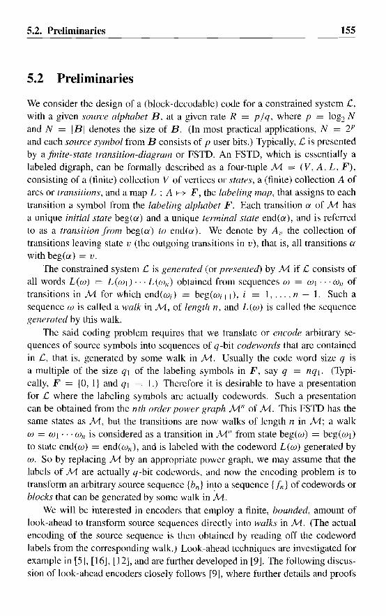
5.2. Preliminaries

5.2 Preliminaries

155

We consider the design of a (block-decodable) code for a constrained system 1:,with a given source alphabet B, at a given rate R = p / q, where p = logz Nand N = IBI denotes the size of B. (In most practical applications, N = 21'and each source symbol from B consists of p user bits.) Typically, I: is presentedby a finite-state transition-diagram or FSTD. An FSTD, which is essentially alabeled digraph, can be formally described as a four-tuple M = (V, A, L, F),consisting of a (finite) collection V of vertices or states, a (finite) collection A ofarcs or transitions, and a map L : A r--+ F, the labeling map, that assigns to eachtransition a symbol from the labeling alphabet F. Each transition a of M hasa unique initial state beg(a) and a unique terminal state end(a), and is referredto as a transition from beg(a) to end(a). We denote by A v the collection oftransitions leaving state v (the outgoing transitions in v), that is, all transitions a

with beg(a) = v.

The constrained system I: is generated (or presented) by M if I: consists ofall words L(w) = L(WI)'" L(wn ) obtained from sequences W = WI'" wn oftransitions in M for which end(wi) = beg(wi+I), i = 1, ... , n - 1. Such asequence W is called a walk in M, of length n, and L(w) is called the sequencegenerated by this walk.

The said coding problem requires that we translate or encode arbitrary se­quences of source symbols into sequences of q-bit codewords that are containedin 1:, that is, generated by some walk in M. Usually the code word size q isa multiple of the size qi of the labeling symbols in F, say q = nql. (Typi­cally, F = {O, I} and qi = 1.) Therefore it is desirable to have a presentationfor I: where the labeling symbols are actually codewords. Such a presentationcan be obtained from the nth order power graph Mil of M. This FSTD has thesame states as M, but the transitions are now walks of length n in M; a walkW = WI ... W n is considered as a transition in Mil from state beg(w) = beg(wI)to state end(w) = end((vn ), and is labeled with the codeword L(w) generated byw. So by replacing M by an appropriate power graph, we may assume that thelabels of M are actually q-bit codewords, and now the encoding problem is totransform an arbitrary source sequence {bn} in.to a sequence {fn} of codewords orblocks that can be generated by some walk in M.

We will be interested in encoders that employ a finite, bounded, amount oflook-ahead to transform source sequences directly into walks in M. (The actualencoding of the source sequence is then obtained by reading off the codewordlabels from the corresponding walk.) Look-ahead techniques are investigated forexample in [5], [16], [12], and are further developed in [9]. The following discus­sion of look-ahead encoders closely follows [9], where further details and proofs

156 5. Bounded delay encodable, block-decodable codes

o(~~[Ol~--------=: b

[-] ~ 1(0)

"",-

1( 1) 1(0)

[1) c 1(1)

Figure 1: A look-ahead encoder.

can be found.An M -symbol look-ahead encoder for M involves a map cp : A r-+ B that

assigns to each transition a of M a source symbol cp(a) from B. The task ofthe encoder is to translate each sequence b l , b2, ... of source symbols into a walkaI, a2, ... in M such that cp(an ) = bn holds for all n.

In the simplest case, M = °(no look-ahead is required) and the pair [M, cp]

constitutes an encoder graph, that is, for each state v and each source symbol b,there is a transition a leaving v with source label cp(a) = b. This transition canthen be used to encode b, by the codeword L(a), if the encoder is presently instate v.

Observe that an encoder graph based on M exists if and only if at least Ntransitions leave each state of M. Even if this is not the case, encoding may stillbe possible by employing look-ahead to avoid entering a state from which theupcoming source symbol(s) cannot be encoded. The encoder is then allowed tobase its choice of the next transition to be included in the encoding path on thepresent source symbol along with the next M upcoming source symbols, for somefixed number M termed the look-ahead of the encoder. Since a state is enteredwith knowledge of the next M upcoming source symbols only (one symbol beingencoded by the entering transition), encoding from this state must be possible forall source sequences starting with these M symbols. Consequently, with eachstate v of the encoder there will be associated a collection of words W v , called thelist ofadmissible prefixes (each member being a source word of length at most M)

specifying the prefixes of sequences of source symbols that can be encoded fromthis state. Consider the following simple example, taken from [9].

Example 1: A typical look-ahead encoder, with source alphabet {a, I}, ispresented in Figure 1. Note that we have not indicated the codeword labels of thetransitions. Throughout this paper, we will adopt the convention that unlabeledtransitions are assumed to be labeled with their terminal state. (The reason for

5.2. Preliminaries 157

this seemingly strange convention is that often the FSTD M representing theconstraint will be in Moore-machine form, with as states the codewords, and withthe transitions from a state indicating which codewords are possible successors tothe codeword associated with this state.) So here, we have F = {a, b, c}.

The encoder has three states, marked a, b, and c. In state a, no requirementson upcoming source symbols are imposed (indicated in Figure 1 by the prefix listW a = [-] containing the empty word only.) State b may be entered only with anupcoming source symbol equal to °(indicated by the prefix list Wb = [OD, andsimilarly, state c has prefix list We = [1]. Each transition in Figure 1 carries asource symbol, sometimes followed by a parenthesized symbol indicating a con­straint on the upcoming source symbol. For example, to encode source symbol 1from state a, the encoder looks ahead at the upcoming source symbol, and choosesthe transition from a to b, labeled 1(0), if this symbol equals 0, or the transitionfrom a to c, labeled 1(1), otherwise. (A similar notation is used e.g. in [16].) Itis easily verified that Figure 1 indeed presents an encoder; encoding of a sourcesequence from an encoder state is possible if the sequence has a prefix containedin the list of admissible prefixes associated with that state. This encoder neveremploys more than one symbol look-ahead, and is therefore called a one-symbollook-ahead encoder.

Finally, we observe that the code is block-decodable: the codeword a alwaysencodes source symbol 0, and both codewords band c always encode sourcesymbol 1. 0

Which conditions must be satisfied by the lists of admissible prefixes Wv inorder that M -symbol look-ahead encoding is indeed possible? To answer thatquestion, we first observe that we may assume without loss of generality that eachlist W v consists entirely of words of length Mover B. (Indeed, replacing W v bythe set of words of length M with a prefix in W v does not affect whether or nota given source sequence has a prefix in W v .) Then, the required condition statesthat for each state v of M, for each word bl ... bM E W v , and for each sourcesymbol b = bAH I from B, there must be a transition a leaving state v such thatcp(a) = h (that is, a encodes bd, and b2 ·· . bM +1 E Wend(a). To understandthe second condition, note that since the encoder bases its choice of transition a

on b l , ... , bM , bM+I only, all source sequences with prefix b2' .. bM+l must beencodable from state end(a).

Conversely, if the lists W v satisfy these conditions and if at least one of thelists is non-empty, then M -symbol look-ahead encoding is indeed possible, asthe reader can easily verify. (Observe that if v is a state for which W v is non­empty, then each source sequence, when prefixed with a fixed word in W v , can beencoded starting from this state v.)

158 5. Bounded delay encodable, block-decodable codes

(1)

It will be convenient to introduce the following notation. We denote by WvBthe set of all words h ... bM +I with bi ... bM E W v and bM+I E B. If cp(a)

denotes the source label of transition a, then we write cp(a)Wend(U') to denotethe collection of all words cp(a)b2'" b M+I with b2" . bM+I E Wend(U'). Thecollection of all subsets of a set X will be denoted by P(X). We can now state thefollowing formal definition of a look-ahead encoder (see [9]).

Definition 1: An M -symbol look-ahead encoder with source alphabet B fora FSTD M consists of a triple [M, cp, W], where cp : A f-+ B denotes a labelingof the transitions with symbols from B, and W : V f-+ P(B M ) is a map whichassigns to each state v of M a collection W v of words of length Mover B, list of

admissible prefixes at v, such that(a) at least one W v is non-empty, and(b) for all states v, we have

WvB s; Ucp(a)Wend(U'),

U'EA"

where A v denotes the set of transitions leaving v.

We will refer to such a map W as an M -symbol look-ahead assignment for M(with respect to cp, or with respect to the partition of the labeling alphabet of Minduced by cp).

In practical applications it is desirable that the decoding decision on a code­word depends on the local context of that codeword only in order to limit errorpropagation. (See e.g. [18].) Codes with that property are termed sliding-block

decodable. We point out that codes that possess a look-ahead encoder [M, cp, W]as in Definition 1 are certainly sliding-block decodable if (the labeling map L of)M is offinite type, that is, if there are numbers m and a, m, a ~ 0, such thatwalks UL m ... wa ... (Va that generate a given word f -m ... fa ... fa all agree intransition Woo The numbers m and a are termed the memory and anticipation of Land M, respectively, We can then reconstruct the walk W- m ... Wa' .. Wn+a usedto generate a given sequence of codewords f -m ... fa ... fn+a in £', except forthe first m and last a transitions. Indeed, each Wk, 0 :::: k :::: n, is determineduniquely by fk-m ... fk ... fHa, the decoding window for the codeword fk. Asa result, !k is decoded as bk, where bk = cp(Wk) is the source symbol associatedwith transition Wk. The number m + 1 + a is termed the decoding-window size ofthe code. It is well-known that a constrained system £, is of finite type (that is, £,

can be generated by an FSTD of finite type) precisely when £, can be specified interms of a finite list offorbidden blocks [1].

We say that a code is block-decodable if the code is sliding-block decodablewith a decoding window of size one codeword, that is, if the decoding decision

5.3. BDB codes 159

on a codeword is independent of preceding and succeeding codewords. Observethat the set of codewords F of a block-decodable code can be partitioned intocodeword classes Fb, b E B, such that a codeword f E F is decoded as sourcesymbol b precisely when f E Fb.

Many code construction methods employ an approximate eigenvector. (Seee.g. [3], [16], [1 ],[9].) Here, a collection of non-negative integer weights cPv, notall zero, associated with the states v of M constitute an [M, N]-approximateeigenvector if, for each state v, the sum of the weights of terminal states of theoutgoing transitions is not less than N times the weight of state v, that is, if

N cPv :s L cPend(OI) (2)OIEA v

holds for each state v. Usually, we think of cP (cPV)VEV as a vector, and theabove condition is stated as

where the inequality is to be interpreted component-wise. Here DM denotes theIVI x IVI adjacency matrix of M; DM(V, w) equals the number of transitionsfrom state v to state w. We quote the following theorem from [9].

Theorem 1: Let [M. cp, W] be an M-symbollook-aheadencoder with sourcealphabet B. Then the weights cPv defined by cPv = IWvl, the size of the list ofadmissible prefixes associated with state v, satisfy 0 :s cPv :s IB IM and constitutean [M, IBI]-approximate eigenvector.

5.3 BDB codes

Informally, a bounded-delay encodable, block-decodable code or BDB code withsource alphabet B for a constrained system £ is a collection of disjoint codewordclasses Fb , b E B, with the property that each source sequence blb2 ... can beencoded into a constrained sequence fl Jz ... in £ with fi E Fbi by a finite­state machine, with a bounded encoding delay, or, equivalently, using a boundedamount of look-ahead.

In a sense, the use of the word "code" is somewhat misleading, since it sug­gest that a BDB code is characterized by its code sequences, while in reality itis characterized by its decoder map (and the fact that bounded-delay encoding ispossible). This point is further discussed in the appendix.

Evidently, an M-symbollook-ahead encoder for an FSTD M with £(M) S;

£ which is block-decodable in fact provides a BDB code for L. We will refer tosuch an encoder as a BDB encoder for M. In the appendix, we present a formaldefinition of BDB codes, together with a proof of the following theorem.

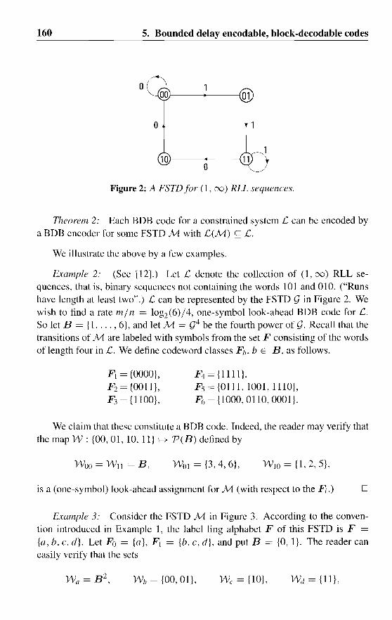
160 5. Bounded delay encodable, block-decodable codes

oOOJ---------jOl

o

1O}----------{ 11o

Figure 2: A FSTD for (1, 00) RLL sequences.

Theorem 2: Each BOB code for a constrained system 12 can be encoded bya BOB encoder for some FSTO M with L(M) ~ £.

We illustrate the above by a few examples.

Example 2: (See [12].) Let 12 denote the collection of (1,00) RLL se­quences, that is, binary sequences not containing the words 101 and 010. ("Runshave length at least two".) £ can be represented by the FSTO 9 in Figure 2. Wewish to find a rate min = log2(6)/4, one-symbol look-ahead BOB code for L.So let B = {1, ... , 6}, and let M = g4 be the fourth power of g. Recall that thetransitions of M are labeled with symbols from the set F consisting of the wordsof length four in £. We define codeword classes Fh , b E B, as follows.

F I = {OOOO},F2 = {001l},F3 = {1100},

F4 = {llll},F s ={0111, 1001, 11l0},F6 = {1000, 0110, 0001}.

We claim that these constitute a BOB code. Indeed, the reader may verify thatthemapW: {00,01, 10, II} ~ P(B) defined by

Woo = Wll = B, WOl = {3, 4, 6}, WIO = {l, 2, 5},

is a (one-symbol) look-ahead assignment for M (with respect to the Fi .) D

Example 3: Consider the FSTO M in Figure 3. According to the conven­tion introduced in Example 1, the label ling alphabet F of this FSTO is F =

{a, b, c. d}. Let Fo = {a}, F I = {b, c, d}, and put B = {O, I}. The reader caneasily verify that the sets

Wh = {OO, Ol}, We = {1O},

5.3. BDB codes

a}--------------j-----{ b

d}------------{ c

Figure 3: The FSTD M for Example 3.

oFigure 4: The FSTD's 9 (left) and M (right) for Example 4.

161

constitute a two-symbol look-ahead assignment for M, hence the Fi constitute atwo-symbol look-ahead BDB code. 0

According to Theorem 2, we might as well have defined a BDB code for aconstrained system £ as the collection of codeword classes of a block-decodablelook-ahead encoder for some FSTD M that generates a constrained system in­cluded in 12. At first, it would seem that such a definition is highly dependent onthe particular FSTD M. Fortunately, this is not the case if the constrained systemis of finite type. Indeed, we have the following theorem.

Theorem 3: Let £ be a constrained system generated by a FSTD M of finitetype. Then, each M -symbol look-ahead BDB code for £ is the collection ofcodeword classes of an (M + a)-symbol block-decodable look-ahead encoderfor M, where a denotes the anticipation of M.

The proof of this result can also be found in Appendix A. As the next exampleshows, this result need not hold if the FSTD is not of finite type. (A more subtleexample that illustrates another limitation of this result is quoted in Appendix B.)

Example 4: Consider the FSTD's 9 and M in Figure 4. Both these FST­D's have labeling alphabet F = {O, I}, and generate the constrained system £consisting of unconstrained binary sequences. Let B = {O, I}, and let Fa = {OJand F j = {l}. Obviously, this partition constitute a (trivial) BDB code for 12;if we let W v = A, where A denotes the empty word over B, then W defines a

162 5. Bounded delay encodable, block-decodable codes-----------------~--

O-symbollook-ahead assignment for g. However, the reader may verify that theredoes not exist a look-ahead assignment for the FSTD M with respect to this par­tition of F. Indeed, an even run of ones followed by a zero can only be encodedby starting with a transition from state a, while an odd run of ones followed by azero can only be encoded by starting with a transition from state b. D

It is well-known (see e. g. [1]) that £, is of finite type precisely then whenits (right) Shannon cover (the "smallest" deterministic FSTD that generates £,)

has finite memory. (Since it is deterministic, it has anticipation a = 0.) Also,constrained systems of finite type are precisely those constrained systems £, thatcan be characterized by a finite list of forbidden words that are not allowed tooccur as sub-words in words of £'. The above theorem then has the followingconsequence.

Theorem 4: Each M -symbol look-ahead BDB code for a constrained systemof finite type is the collection of codeword classes of a block-decodable M -symbollook-ahead encoder for its (unique) right Shannon cover.

The above results have some interesting theoretical consequences. Let usagree to call a code construction method universal for a class of constrained sys­tems and for codes of a certain type for such systems if each such code for eachsuch system can in principle be obtained by use of the method. The code sys­tem of a code is the collection of all possible encoded sequences produced by theencoder for the code. It is now possible to show the following.

Theorem 5: Both the ACH state-splitting method and the BD-method in [9]are universal for sliding-block decodable codes of constrained systems of finitetype that have a finite-state encoder with a finite-type code word labeling. More­over, both methods can construct any given sliding block-decoder of codes forconstraints of finite type. Here, the constructed encoder may have a code systemdifferent from the code system of the given code in the case that this code systemis not of finite type.

Since both the BD method and the ACH algorithm transform graphs of finitetype into graphs that are again of finite type, the above theorem can be interpretedas stating that both methods are capable to construct everything that is not a-prioryimpossible.

In what follows we give a sketch of the proof of this claim. (Details con­cerning the more subtle points of this theorem are given in Appendix B.) The keyobservation is that a sliding-block decodable code with window size T for a con­strained system £, generated by a FSTD M is equivalent to a block-decodablecode for the Tth higher block system £'T generated by the Tth order edge-graphM[T] of M(see e.g. [1]). Now the claim for the BD method follows from the

5.3. Principal state-sets 163

above results together with the observations in [9, Section 2]. The correspondingclaim for the state-splitting method follows from the equivalence of the two meth­ods as shown in [9, appendices] (see also Chapter 4, Appendix C). Most of theabove claims for the state-splitting method was also proved in [2] by other means.

5.4 Principal state-sets for one-symbol look-ahead BDBcodes

In this section and the next one, we shall describe our first construction methodfor BDB codes. The method is universal, in the sense that each BDB code canthus be constructed. This section covers the case of one-symbol look-ahead BDBcodes, and serves as an introduction to the more general case.

Let M = (V, A, L, F) be a FSTD, generating the constrained system ,c,say. Let {Fh}bEB be a partition of the labeling alphabet F of M. Suppose thatsomebody claims that the Fh, b E B, constitute the codeword classes of a (one­symbol look-ahead, say) BDB code for 'c. How could we verify this? Of course,one method would be to find lists of admissible prefixes for all states of M, butthis may be difficult. We will now describe an alternative method.

Let E denote a collection of non-empty subsets of the state-set V of M. Wewill commonly refer to members of E as principal state-sets. As will becomeclear later on, this notion generalizes the concept of principal states as introducedby Franaszek [3]. A subset C S; F will be called a codeword class with respectto E if for each principal state-set E E E we can find a state e in E such that thecollection of C -successors of e in M contains a principal state-set E' in E. Here,a state v of M is a C-successor of state e if there is a transition in M from e to vwith label contained in C. Now we have the following result.

Theorem 6: Let M = (V, A, L, F) be a FSTD that generates a constrainedsystem'c. Let Ct, ... , CN be mutually disjoint subsets of F, and suppose thateach Ci is a codeword class with respect to some given collection E of non-emptysubsets of the states of M. Then the Ci are the codeword classes of a one-symbollook-ahead BDB code for ,c with source alphabet B = {I, ... , N}.

Proof Think of a (principal state-set) E from E as representing states end(a)of a collection of transitions a from some (earlier determined) state v in M forwhich L (a) S; Ci is a feasible coding alternative for a given source symbol i in B.Let b E B be the upcoming symbol to encode. Since Ch is a codeword class withrespect to E, there is a state e in E such that the collection of Ch-successors of econtain a set E' from E. We now encode i as L(f3), where fJ is a transition from vto e with label contained in Ci. Now continue the encoding with e and E'. 0

164 5. Bounded delay encodable, block-decodable codes

Example 5: Consider again the collection F'b, b = 1, ... , 6, from Example 2.Let E = {E l , E 2 , E3}, where

E l = {OO}. E2 = {ll}, E3 = {aI, 10}.

It is not difficult to verify that the Fb are codeword classes with respect to thiscollection E of principal state-sets. Since the Fb are obviously disjoint, they con­stitute a'one-symbollook-ahead BDB code according to Theorem 6. Moreover, itis easily verified that the sets

F7 = {Olll, lOOO}, Fs = {OllO, 0001, 1110, 1001}

are also codeword classes with respect to E. Consequently, F], ... , F4 , F7 , Fsconstitute a second BDB code. 0

Example 5 (see also Example 7) illustrates a nice property of the description ofa BDB code in terms of principal state-sets: If, from a good hunch, or by any othermeans, we "guess" to start with some "good" collection E of principal state-sets,then we may mechanically list all codeword classes with respect to E, and justpick out the largest possible (or a very large) collection of mutually disjoint ones.This latter task, SET PARTITIONING, is computationally difficult ("NP-hard")in general, but can nevertheless be solved in many cases, even for rather largesource alphabets. (This last point is exemplified by [10], see also Example 7.)

We will discuss methods to obtain "good" collections of principal state-setswhen we relate this method to the method of state combination as described byImmink [12].

Our next result shows that each one-symbol look-ahead BDB code can beobtained from a suitable collection of principal state-sets. In order to state thisresult, we introduce some new notation. Let M = (V, A. L, F) be a FSTD, andlet W v , v E V, denote a collection of admissible prefix lists for a one-symbollook-ahead BDB encoder for M with respect to a partition {Fb}bEB of F. Foreach state v of M and for each symbol b from W v , let E(v, b) denote the collec­tion of all states of the form end(a) with a a transition of M with beg(a) = vand L(a) E F),. We denote the collection of all these sets E(v, b) by E(W).

Theorem 7: With the above notation, each Fb, b E B, is a codeword classwith respect to the collection E(W).

Proof Let c E B. We will show that Fc is a codeword class with respectto E(W). So let E(v, b) E E(W), that is, bE W v ' By the properties of W, thereis a transition a from v to a state w = end(a) with L(a) E F c for which c E W w '

Hence w E E(v, b) and the set E(w, c) E E(W) is defined and is contained in (infact, equal to) the collection of Fc-successors of w. 0

5.4. Principal state-sets 165

The construction method suggested by Theorem 6, which we will call theprincipal state-set method, may be considered as a generalization of the methodto construct block codes through principal states. In that case, all principal state­sets consist of a single state only, and the resulting BDB codes are block codes,that is, encoding requires no look-ahead at all. Further relations with the work ofFranaszek on Bounded Delay codes ([3]-[6]) will be discussed in a later section.

The principal state-set method offers further advantages when one is lookingfor (large) one-symbol look-ahead BDB codes for a given constrained system, forvarious block-lengths n, that is, for BDB encoders for gn for various values of n,where g is a FSTD that describes the constraint. We illustrate this for the case of(I, (0) RLL sequences in our next example. (See [13] for further examples of thiskind.) .

Example 6: Consider again the FSTD g in Figure 2 that describes the O. (0)RLL constraint. For n :::: 4, let M = gn be the nth power of g. (So the transitionsin M are labeled with admissible words of length n.) Let E denote the collectionof principal state-sets as in Example 5. In order to decide if a given set C of wordsof length n is a codeword class with respect to E, it is sufficient to know the typeof each word in C, that is, the first two and the last two symbols of each word,since these four symbols determine the successor relations and terminal states oftransitions labeled with this word.

We say that an admissible word x = Xl' .. X n has begin type XIX2, end type

Xn-]Xn and type XIX2-Xn-IXn. Admissible words of length at least four are ofsixteen different possible types. (When dealing with an arbitrary constrained sys­tem £ of finite type, the begin- and end-types of long enough words are states inthe left- and right-Shannon cover for £, respectively.) The class type of a set ofadmissible words C of length n is the collection of types of words in C, and theclass type of C is a codeword class type with respect to E if C (and hence also anyother collection C' of words of the same class type as C) is a codeword class withrespect to E.

It turns out that there are precisely 47 distinct inclusion-minimal codewordclass types with respect to E. Moreover, it is possible to derive expressions thatenumerate admissible words of length n of a given type. Using these results, it canbe shown that for each value of n with n :::: 4 there is a one-symbol look-aheadBDB encoder for M = gn with N(n) codeword classes, where

N(n) = LFn+3/2J = Fn+l + LFn/2J. (4)

In the above expressions, F" denotes the nth Fibonacci number, defined by FI =F2 = I and Fn = Fn- l + Fn~2 for n :::: 3. Further details can be found in a future

166 5. Bounded delay encodable, block-decodable codes

paper [13]. In that paper it is also shown that no BDB code for this constraint andwith block length n can have more than N (n) codeword classes.

Observe that the case n = 4, N(n) = 6, is the subject of Examples 2 and 5.We also observe that, since N (6) = 17, there is a (1. (0) RLL BDB code withrate m / n = 4/6. We will return to this case in the next section. D

Example 7: This example concerns (1, 8) RLL BDB codes. The commonFSTD for this constraint (which is in fact the Shannon cover) has states 01 i andWi, 1 ::: i ::: 9. As principal state-sets, we choose the following collections.

2 ::: i ::: 4,2 ::: i ::: 4,

{IO. aI},{Ol i, Wi}, 5::: i, j ::: 9, (i, j) i- (9,9).

In [10] we describe a one-symbol look-ahead rate min = 8/12 BDB codefor this constraint with as principal state-sets the above collection. In fact, thispaper lists a number of codeword class types, and then some counting shows thatsufficiently many disjoint codeword classes of these class types can be formed.The same principal state-sets and codeword class types could be used for othervalues of the block-length n as well, as long as n ::: 9. (This last condition ensuresthat a forbidden word is confined to two consecutive codewords.) The results inthat paper also show that some further simplifications in the search for codewordclass types are possible. D

We now discuss the problem of how to find a "good" collection of principalstate-sets for a given FSTD jvL Our main method is based on (approximate)eigenvectors of the adjacency matrix DM cOlTesponding to M. Intuitively, this isappealing since a component of such a vector reflects in some way the amount ofinformation that can be encoded from the cOlTesponding state.

Unfortunately, these methods can only serve as a guideline, and some creativ­ity is still required. An interesting and related method is the following. Supposewe try to find a code with N codeword classes. First, we construct an [M, N]­approximate eigenvector ¢ with all components equal to zero, one, or two. Thenwe run the state combination method as described in [12] with M and ¢ to obtain"good" state combinations. Finally, we use the state combinations thus obtainedas our collection of principal state-sets. In a later section we relate the state com­bination method to our work and give some more details on the above method.

5.5 State-trees for M-symbol look-ahead BDB codes

In this section we generalize our previous results for the case where M = 1 to allvalues of M. As before, we let M = (V, A, L, F) denote a FSTD representing a

5.5. State-trees for M -symbol look-ahead BDB codes

E1: .e-_---<e e a

167

E':~: c

d

Figure 5: Three state-trees.

constrained system £, we let {Fb }bEB denote a partition of the labeling alphabet Fof M, and W : V ~ P(BM ) denotes an M-symbollook-ahead assignment forM with respect to this partition. So the Fb are the codeword classes of an M­symbol look-ahead BDB encoder for M (or for £) with source alphabet B.

In the previous section we defined the sets E (v, b), v E V, b E Wv, for thecase where M = 1. We think of such a set as a rooted directed tree (with rootcorresponding to the state v) of depth one (all walks from the root to a sink, thatis, a vertex in the tree without successors, have length one), with sinks labeledwith states of M. It is this structure that we intend to generalize.

We define a state-tree for M to be a rooted directed tree in which all walksfrom the root to a sink have the same length D, for some number D ::::: 0, withsinks labeled with states from M. The number D is the depth of the state-tree.(In the case where D = 0, the state-tree consists of a single vertex, labeled witha state of M, with no arcs.) A vertex s of a state-tree E has depth K in E if the(unique) walk in E from the root to s has length K.

Example 8: Consider again the FSTD M in Figure 3. In Figure 5 we havethree state-trees for M, each of depth two. D

In what follows, we will use collections of state-trees to construct BDB en­coders for M, just as we did in the previous section with collections of principalstate-sets. As before, the idea is to use the state-trees as "states" of the encoder,and to move from encoder state to encoder state according to upcoming codewordclasses, in such a way that the resulting encoder state sequence defines a walkin M with a "correct" labeling. We think of a state-tree as describing in someway the collection of walks in M that are feasible encoding alternatives at a givenencoding moment.

First we explain how to move from one state-tree to another. The idea is verysimple, but a precise description is a bit complicated. Therefore, we first presenta suggestive example.

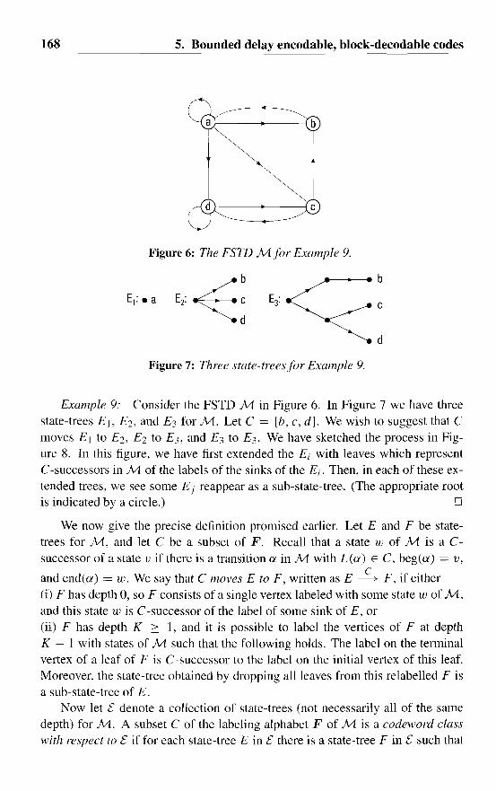
168 5. Bounded delay encodable, block-decodable codes

ar---~

d }----------( c

Figure 6: The FSTD M for Example 9.

..._-- b

c

d

Figure 7: Three state-trees for Example 9.

Example 9: Consider the FSTD M in Figure 6. In Figure 7 we have threestate-trees E1, E2, and E3 for M. Let C = {b, c, d}. We wish to suggest that Cmoves E 1 to E2, E2 to E3, and E3 to E3. We have sketched the process in Fig­ure 8. In this figure, we have first extended the Ei with leaves which representC-successors in M of the labels of the sinks of the Ei . Then, in each of these ex­tended trees, we see some E j reappear as a sub-state-tree. (The appropriate rootis indicated by a circle.) 0

We now give the precise definition promised earlier. Let E and F be state­trees for M, and let C be a subset of F. Recall that a state w of M is a C­successor of a state v if there is a transition a in M with L(a) E C, beg(a) = v,

and end(a) = w. We say that C moves E to F, written as E ~ F, if either(i) F has depth 0, so F consists of a single vertex labeled with some state w of M,and this state w is C-successor of the label of some sink of E, or(ii) F has depth K :::: 1, and it is possible to label the vertices of F at depthK - 1 with states of M such that the following holds. The label on the terminalvertex of a leaf of F is C-successor to the label on the initial vertex of this leaf.Moreover, the state-tree obtained by dropping all leaves from this relabelled F isa sub-state-tree of E.

Now let E denote a collection of state-trees (not necessarily all of the samedepth) for M. A subset C of the labeling alphabet F of M is a codeword classwith respect to E if for each state-tree E in E there is a state-tree F in E such that

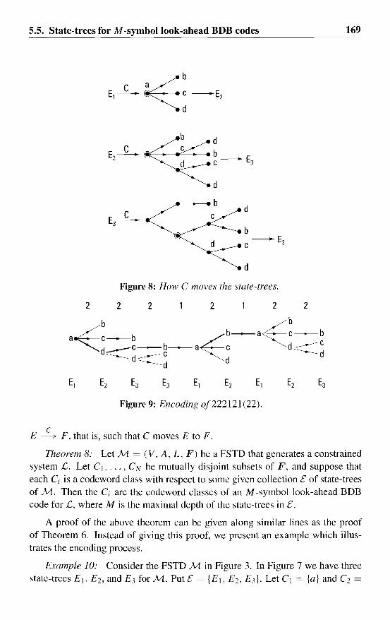
b

5.5. State-trees for M -symbol look-ahead BDB codes

dCEz--- c~------,-::-----.b

c --- E3

169

d

A_-_bc

d

b---E3C

d

Figure 8: How C moves the state-trees.

2 2 2 2 2 2

E, E, E,

Figure 9: Encoding of222121(22).

E~ F. that is, such that C moves E to F.

Theorem 8: Let M = (V, A, L, F) be a FSTD that generates a constrainedsystem £. Let C1, ... , CN be mutually disjoint subsets of F, and suppose thateach Ci is a codeword class with respect to some given collection E of state-treesof M. Then the Ci are the codeword classes of an M-symbollook-ahead BDBcode for £, where M is the maximal depth of the state-trees in E.

A proof of the above theorem can be given along similar lines as the proofof Theorem 6. Instead of giving this proof, we present an example which illus­trates the encoding process.

Example 10: Consider the FSTD M in Figure 3. In Figure 7 we have threestate-trees EI, E2, and E3 for M. Put E = {E I, E2, E3}. Let Cl = {a} and C2 =

170 5. Bounded delay encodable, block-decodable codes

00E,:<01Figure 10: Four state-trees for Example 11.

{b, c, d}. It is easily verified that the C are codeword classes with respect to E.(In Example 9 this is verified for C2, since the transition from c to d in the FSTDin Figure 6 is never required.) According to Theorem 8, CI and C2 constitute atwo-symbol look-ahead BDB code for the constrained system generated by M,with source alphabet B = {I , 2}. In Figure 9 we show the process of encoding thesource sequence 222121 (22), starting from state-tree E I. The heavy line indicatesthe walk in Ai taken by the encoder. Consequently, the sequence 222121 (22)encodes as dcbaba. D

We will now show that, as expected, each BDB code arises from a collectionof state-trees. Indeed, given an M -symbol look-ahead assignment W for M, wemay construct for each state v of M and for each b = bl ... bM in W v a state-treeE (v, b) as follows. The vertices of E (v, b) may be identified with those walksWI ... Wk in M which generate the word h ... bk, for k = 0, ... , M, with an arcfrom WI" . Wk to WI" . WkWHI if both walks correspond to vertices of E(v, b).(So the root corresponds to the empty walk in M.) Finally, a vertex at depth Mcorresponds to a walk WI ... WM in M that generates bl ... bM and is labeled withthe state end(wM) in M. We denote the collection of all state-trees E(v, b) with va state of M and bE W v by feW). We now have the following.

Theorem 9: Let M = (V, A, L, F) be a FSTD, and let W denote an M­symbol look-ahead assignment for M with respect to a partition {FblbEB of F.Then each Fb, b E B, is a codeword class with respect to the collection of state­trees feW).

The construction method suggested by Theorem 8 will be referred to as thestate-tree method. Everything that was said about the principal state-set methodcan be repeated here for the state-tree method.

In the remainder of this section, we will illustrate the state-tree method for theconstruction of BDB codes by some examples concerning BDB codes for (d, k)RLL sequences. As remarked earlier, "optimal" BDB codes for the (1, (0) RLLconstraint require at most one-symbol look-ahead. We wonder if the same is truefor other values of d and k as well. In fact, at first it is not at all evident that thereare BDB codes for these constraints that require more than one-symbol look-aheadat all. Our next example presents such a BDB code.

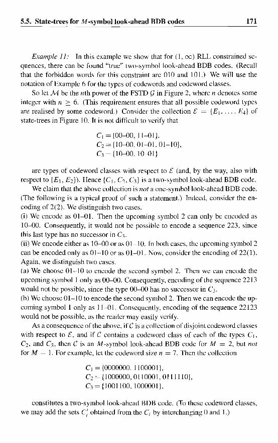
5.5. State-trees for M -symbol look-ahead BDB codes 171

Example 11: In this example we show that for (1, (0) RLL constrained se­quences, there can be found "true" two-symbol look-ahead BDB codes. (Recallthat the forbidden words for this constraint are 010 and 101.) We will use thenotation of Example 6 for the types of codewords and codeword classes.

So let M be the nth power of the FSTD 9 in Figure 2, where n denotes someinteger with n :::: 6. (This requirement ensures that all possible codeword typesare realised by some codeword.) Consider the collection £ = {E I , •.. , E4} ofstate-trees in Figure 10. It is not difficult to verify that

C, = {OO-OO, 11-01},C2 = {1O-00, 01-01, 01-10},C3 = {10-00, 1O-01}

are types of codeword classes with respect to £ (and, by the way, also withrespect to {EI, E2}). Hence {CI, C2, C3} is a two-symbol look-ahead BDB code.

We claim that the above collection is not a one-symbol look-ahead BDB code.(The following is a typical proof of such a statement.) Indeed, consider the en­coding of 2(2). We distinguish two cases.(i) We encode as 01-01. Then the upcoming symbol 2 can only be encoded as10-00. Consequently, it would not be possible to encode a sequence 223, sincethis last type has no successor in C3.

(ii) We encode either as 10-00 or as 01-10. In both cases, the upcoming symbol 2can be encoded only as 01-10 or as 01-01. Now, consider the encoding of 22(1).Again, we distinguish two cases.(a) We choose 01-10 to encode the second symbol 2. Then we can encode theupcoming symbol 1 only as 00-00. Consequently, encoding ofthe sequence 2213would not be possible, since the type 00-00 has no successor in C3.(b) We choose 01-10 to encode the second symbol 2. Then we can encode the up­coming symbol 1 only as 11-01. Consequently, encoding of the sequence 22123would not be possible, as the reader may easily verify.

As a consequence of the above, if C is a collection of disjoint codeword classeswith respect to £, and if C contains a codeword class of each of the types CI,

C2, and C3, then C is an M-symbol look-ahead BDB code for M = 2, but notfor M = 1. For example, let the codeword size n = 7. Then the collection

C I = {OOOOOOO, 1100001},C2 = {1000000, 0110001, 0111110},C3 = {l 001100, 1000001},

constitutes a two-symbol look-ahead BDB code. (To these codeword classes,we may add the sets C; obtained from the Ci by interchanging 0 and 1.)

172 5. Bounded delay encodable, block-decodable codes

Figure 11: The state-trees for Example 12.

Due to the symmetry 0 *-+ 1 of the collection £ of state-trees, there areevidently many other codeword class types. It is therefore possible to obtain rea­sonably large codes, although of course not larger than the codes in Example 6,since these are optimal. 0

Example 12: Here we consider rate 2/3 (1, k) RLL codes with codewordsize n = 6. The following 17 codeword classes partition the 26 words of lengthsix that do not contain 010 or 101.

Cj = {OOOOOO},C2={IllIll},C3 = {OOllOO},C4 = {1l001l},Cs = {I I 1100},C6 = {OOOOII},C7 = {0001l1},Cs = {llIOOO},C9 = {OOlIlI},

C10 = {l10000},CII = {000001. 0001l0},C12={1l1001,IIllIO},C13 = {O 11100, 100000},CI4 = {OIl 111, 10001 I},CIS = {lOOIll, OIlOOO}.CI6 = {I10001, OllIlO, lOOllO},Cn = {OOIIlO, 10000l,OI100]}.

It is not difficult to verify that these 17 codeword classes constitute a one­symbol look-ahead BDB code. with respect to the collection of principal state­sets {OO}, {ll}, and {O], 10}.

Next, we combine CI and C2 to form a new codeword class

C' = {OOOOOO, IllllI},

and we consider the collection of 16 codeword classes C = {C'. C3, ... , C 17 }.We claim that C is a one-symbol look-ahead BDB (1, k) RLL code for k = 11,but not for k = 10. (Additional forbidden words are 0 13 and 113 .) Indeed, thereader may verify that each member of C is a codeword class with respect to thecollection of principal state-sets

{1O.0I}, {lot 2:::: i :::: 7, {Olt 2:::: i :::: 7.

Moreover, we claim that C is a two-symbol look-ahead BDB (1, 10) RLLcode. Indeed, the reader may verify that each member of C is codeword class withrespect to the collection of state-trees in Figure 11.

5.6. The state combination method 173

Finally, we show that we can do equally well with a one-symbol look-aheadBDB code. So, let

Ci = {OOOOOO, OllOOO}, C~ = {llllll, IOOIII},

and let C' = {Ci, c~, C3 .... , C14, C16, Cl7}' The members of C' are mutuallydisjoint and are codeword classes with respect to the collection of principal state­sets

{1O,OI}, {lot 2::: i ::: 6,

Consequently, C is a one-symbol look-ahead BDB (1, 10) RLL code. D

Based on the above examples and many others, we offer the following conjec­ture. Let Mil (d, k) denote the maximum size of a BDB code with codeword sizen for the (d, k) RLL constraint.

Conjecture 1: For all n, d, and k, MIl(d, k) is realized by a BDB code withlook-ahead at most one.

(In a later section we describe an example showing that there may be largerblock-decodable codes. But encoding that code requires an unbounded amount oflook-ahead.) A similar conjecture may be stated for the case of (d, k)-constrainedsequences, that is, binary sequences in which each run of zeroes has a lengthbetween d and k. For d = 1, this has been proved in [8]. Indeed, we do not knowan example of a BDB code for this constraint with a larger size than the (known)optimal size of a block code (that is, a zero-symbol look-ahead BDB code). Thesetwo types of constraints are of course strongly related, and the same may be truefor these two conjectures.

5.6 The state combination method

In this section we introduce an extension of the state combination method to con­struct BDB codes described in [12] (see also [11]). We link this method to ourwork, and we show that each BDB code may be constructed by state combination.

Both state combination and its well-known counterpart state splitting ([1]) aremethods to transform a FSTD representing a given constrained system, with asultimate goal to obtain a representation suitable for encoding purposes. However,the two methods differ in one important aspect: while the new FSTD obtainedfrom state splitting still represents the same constrained system, this is not quitetrue for state combination. What is retained is a one-to-one correspondence be­tween walks in the old and the new FSTD, and thus, also between words generated

174 5. Bounded delay encodable, block-decodable codes

by these FSTD's. Moreover, this correspondence acts as a kind of "built-in" en­coding delay, as we will see.

So let M = (V, A, L, F) denote a FSTD, representing the constrained sys­tem £: = £:(M), and let V = {UI, ... , up} be a collection of states of M. Astate combination with V in M transforms M into a new FSTD M' by addingone new state, also denoted by V, to M. The transitions involving this new state,and their corresponding labels, are the following.(i) Each transition in M from some state in V to some state v not in V producesa transition in M' from state V to v carrying the same label.(ii) Each collection of p transitions in M from a state v to each of the statesUi in V produces a transition in M' from v to state V with as label the set{fl, ... , fp}, where fi denotes the label of the transition in M from v to Ui·Moreover, if v is contained in V, then M' has also a transition from V to V withlabel {fl, ... , fp}·We observe that if the set V consists of a single state, then state combinationwith V essentially duplicates this state and all transitions involving it.

Now let VI, ... , Vk, Vi ~ V, be sets of states of M. A round of statecombinations with VI, ... , V k on M consists of transforming M by successivestate combinations with VI, V 2, ... , V k (it does not matter in which order thesestate combinations are executed, as the reader may easily verify), followed byelimination of all original states of M. Let M be obtained from M by a round ofstate combinations with V I, ... , V k . The following proposition summarizes themain properties of M.

Proposition 10: (i) The FSTD M has a transition from Vi to Vi with labelE if and only if there is a state U in Vi and for each state w in Via transition Wwfrom U to w such that E = {L(ww) I W E Vi}.(ii) Each walk Wj ... Wk+1 of length k+ 1 in M uniquely determines a correspond­ing walk WI' .. Wk of length k in M with the property that beg(Wi) E beg(Wi),end(Wi) E end(wi), and L(wd E L«(Vi), i = I, ... , k, where i(Wi) denotes thelabel of the transition Wi in M.

Example 13: Consider again the FSTD M in Figure 3. One round of statecombinations with {a}, {b}, and {c, d} on M transforms M into the FSTD M'in Figure 12. Then a second round of state combinations, now with {{a}} and{{b}, {c, d}}, transforms M' into the FSTD Mil in Figure 13. D

The built-in encoding delay referred to earlier is illustrated by part (ii) of theabove proposition. In fact, we can say more. With M as in Proposition 10,the result of one round of state combinations applied to M, let M* be a FSTDobtained from M by discarding possibly some of the transitions. A partition

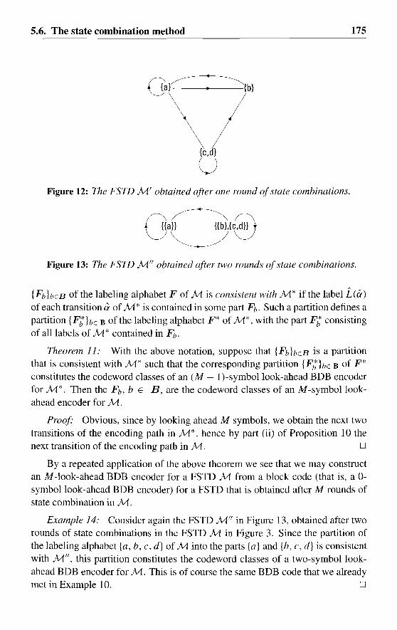
5.6. The state combination method

Qa~1b}\/{C,!U

Figure 12: The FSTD M' obtained after olle round ofstate combinations.

175

Figure 13: The FSTD Mil obtained after two rounds ofstate combinations.

{Fb}bEB of the labeling alphabet F of M is consistent with M* if the label t(a)of each transition aof M* is contained in some part Fb- Such a partition defines apartition {F;}bE B of the labeling alphabet F* of M *, with the part F; consi stingof all labels of M * contained in Fb .

Theorem 11: With the above notation, suppose that {Fb}bEB is a partitionthat is consistent with M* such that the corresponding partition {F/nbE B of F*constitutes the codeword classes of an (M - l)-symbollook-ahead BDB encoderfor M*. Then the Fb, b E B, are the codeword classes of an M-symbollook­ahead encoder for M.

Proof Obvious, since by looking ahead M symbols, we obtain the next twotransitions of the encoding path in M *. hence by part (ii) of Proposition 10 thenext transition of the encoding path in M. D

By a repeated application of the above theorem we see that we may constructan M -look-ahead BDB encoder for a FSTD M from a block code (that is, a 0­symbol look-ahead BDB encoder) for a FSTD that is obtained after M rounds ofstate combination in M.

Example 14: Consider again the FSTD Mil in Figure 13, obtained after tworounds of state combinations in the FSTD M in Figure 3. Since the partition ofthe labeling alphabet {a, b. c, d} of M into the parts {a} and {b, c, d} is consistentwith Mil, this partition constitutes the codeword classes of a two-symbol look­ahead BDB encoder for M. This is of course the same BDB code that we alreadymet in Example 10. D

176 5. Bounded delay encodable, block-decodable codes

State combination as proposed in [12] is a special case ofthe above where Mis of Moore type with all state labels distinct, and where a state of M is usedat most once in a combination, that is, the sets U i representing the states to becombined are mutually disjoint; a state that is used in a state combination is elim­inated immediately afterwards. Moreover, [12] only considers one round of statecombinations. We refer to this paper for further examples.

We will now show that, conversely, each BOB encoder for a FSTO M maybe obtained from rounds of suitable state combinations. So let [M, cp, W] de­note an M -symbol look-ahead BOB encoder, with M ::: l, for a FSTO M =

(V, A, L, F) with respect to the partition {Fb}bEB of the labeling alphabet F

of M induced by cpo Let v be a state of M and let b = bl ... bM be a word invVv . By the defining properties of W, we can find for each b E B a transitionab from v to a state Wb with L(a) E Fh l and b2' .. b!vfb E WW/J' Let U(v, b)denote the collection of all the states Wb thus obtained. We write U(W) to denotethe collection of all these sets U(v, b).

Theorem 12: With the above notation, let the FSTO M be obtained from oneround of state combination on M with the sets contained in U(W). Then we canfind an (M - l)-symbollook-ahead BOB encoder for the FSTO M* obtained byeliminating certain transitions in M.

Proof We begin by describing the FSTO M*. A transition in M from Xto Y, X, Y E U(W), with label E, is retained in M* if there are states v, W

in M and bl, bM+l in B such that b l ... bM E WI" b2 ... bM+I E Ww,X = U(v, b] !Jt,.f)' y = U(w, b2 ··· bM+l), W E X, and E = {L(ab) Ib E B}, where ab is a transition from W to a state u E Y with L(a) in Fb2

and b3 ... bM+1b E Wend(O'/J)' Observe that the labeling set E of this transitionof M* satisfies E ~ Fh2' As a consequence, the given partition of F is consistentwith M*.

For X a state of M*, we define W; to consist of all words b· .. bM for whichX = U(V,blb2···bM)forsomestatevandsomeb] withb l b2 ···bM E WI" Weclaim that these sets W~ constitute an (M - l)-symbollook-ahead BOB encoderfor M*, with respect to the partition of the labeling alphabet of M* induced bythe original partition of F. Indeed, let X E U(W), b2' .. bM E W;. and bE B.Let v and bl be such that b] ... bM E W v and X = U(v, b l ... bM ). Let a bea transition in M with beg(a) = v, L(a) E FbI' and b2 ... bMb E W w , wherew = end(a) (such a transition exists by the defining properties of W). Then, as thereader may easily verify, M* has a transition from X to Y = U(w, b2 · .. bMb),

with label contained in Fhl' and b3 ... bMb E W; by definition of W;. 0

We remark that the statement of Theorem 12 also holds with U (W) replacedby the collection U'(W) consisting of all sets U'(v, b), v E V, b E B, where

5.7. Stable state-sets 177

UI(v, b) is the set of all states end(a) with beg(a) = v and L(a) E Fh. However,it can be shown that U (W) ~ U (W), and each set in U (W) is a union of setsinU(W).

Example 15: Let M be the FSTD in Figure 3, and let W be as in Example 3.If we apply the state combination described in Theorem 12 to M, we obtain theFSTD M I in Figure 12. (If we use state combination with the collection U (W)instead, then we obtain a superfluous state {b, c, d}.) A second application of The­orem 12, using the look-ahead assignment W*, produces the FSTD Mil in fig­ure 13. The two rounds of state combinations are identical to the ones describedin Example 13. 0

Example 16: Let M denote the fourth power of the FSTD in Figure 2. Weleave it to the reader to verify that a round of state combinations with {OO}, {ll},

and {OJ, 1O} on M, followed by the elimination of some of the transitions, canproduce the one-symbol look-ahead BDB codes in Example 2 and Example 5.

As an alternative, we may also obtain these codes from state combination onthe FSTD with as states the admissible words of length four for the (l, (0) RLLconstraint and with the obvious transitions. This is the way in which these codesare constructed in [12]. 0

Although the result in Theorem 12 is satisfactory from a theoretical point ofview, it is not evident how to apply this result for the purpose of code construc­tion. The main problem is of course to know which state combinations are useful.The results from [12] show however that good results can already be obtainedby using only a very restricted set of state combinations, guided by an appropri­ate approximate eigenvector. (On the other hand, it can be shown that the BDBcode in Example 12 cannot be constructed by the methods of [12], so some exten­sion of these ideas is needed.) Moreover, we are also hampered by the followingproblem: Given a FSTD M and a number N, there is no easy way to determinewhether or not there exists a a-symbol look-ahead BDB encoder for M of sizeN. (This problem has been shown to be NP-complete in [20].) Again, in thecase where M is obtained from state combinations on some other FSTD, the re­sults from [12] show that as long as the increase of the number of states is small,the above search problem (refelTed to as the source-to-state assignment problemin [12], section 3.2.1) can often be handled.

5.7 Stable state-sets

Let M = (V, A, L, F) be a FSTD, and let {Fh}hEB denote a fixed partition ofthe labeling alphabet F of M. A natural question is to ask whether this parti-

178 5. Bounded delay encodable, block-decodable codes

tion constitutes the codeword classes of a BDB encoder for M, that is, whetherthere exist admissible prefix lists for the states of M with respect to this partition.Sometimes this problem is easy.

Example 17: In this example, we consider a code for the (1. (0) RLL con­straint with word length n = 3. So let M denote the third power of the FSTDin Figure 2, and consider the following partition of the labeling alphabet of M.

F I = {OOO},F2 = {Ill},

F3 = {OIl, 100},F4 = fOOl, 110}.

It is easily verified that the Fj are the codeword classes of a code, encod­ing of which requires an unbounded amount of look-ahead. Indeed. consider theencoding of 444· . ·4x, where x is either 1 or 2. Since both 001 and 110 can­not succeed themselves, a sequence of fours has precisely two encodings, namely001.110.001. ... and 110.001.110... " one ending in 001 (so that x = 1 next can­not be encoded) and the other ending in 110 so that x = 2 cannot be encoded).

o

However the problem becomes complicated if the number of parts gets large.The question can also be handled if we specify beforehand the maximum amountof look-ahead that may be used, by a method similar to the one in Example 11.But for all that we know the required amount of look-ahead may be larger thanthis maximum. Fortunately, this problem can be solved. We shall show that foreach BDB code there exists a unique inclusion-maximal collection of stable state­sets such that encoding can be described as moving from one stable state-set to thenext. employing a variable but bounded amount of look-ahead. (In the case of one­symbol look-ahead BDB codes, the principal state-sets associated with the codeare all stable state-sets.) Conversely, if we can find a collection of stable state-setsfor our partition, then this partition constitutes a BDB code. As a consequenceof this description, we show the existence of a number M, depending only on thenumber of states IV I of M, such that a BDB encoder for M requires a look-aheadof at most M symbols.

We introduce some additional notation. If W = Wj .•• W n is a walk in M, thenwe say that the walk W generates the word b = bl ... bn over B if L(wd E Fbi'

for all i. We may in fact consider the walk W as a walk in the FSTD M* =(V, A, £*, B) obtained from M by replacing the label of each transition a by£*(a) = b(a), where b = b(a) denotes the (unique) symbol in B for whichL (a) E FI). For two subsets X, Y of the state set V of M and for a word b =b l ... bn over B, we write X -.!!...". Y if there is a state x E X and a walk from xto each state y in Y that generates b. Moreover, we let Xb denote the collection

5.7. Stable state-sets 179

of all states in M that can be reached from X by a walk in M that generates b.Our first result is an easy consequence of the definitions. We leave the proof tothe reader.

Proposition 13: Let X, y, and Z be subsets of V, and let band c be wordsb. e be

over B. If X ----+ Y and Y ----+ Z, then X ----+ Z.

A collection 5 of (nonempty) subsets of the state set V of M is stable withrespect to the given partition of F if for each X in 5 and for each sequence b I b2 ...

over B there is a set Y in 5 and an integer n ~ 1 such that X b~n Y holds. Ifthere always is such an n with n ::: K, then 5 is called K -stable. We refer tomembers of a stable 5 as stable state-sets. We will speak simply of a stablecollection 5 if it is clear from the context to which partition we refer. Our nextresult also follows immediately from the definitions.

Proposition 14: (i) If 5 is stable and if X S; Y, X E 5, then the collection5 U {Y} is again stable.(ii) If 51 and 52 are stable, then the union 51 U 52 is again stable.

By Proposition 14, there either exists a unique inclusion-maximal collectionof stable state-sets with respect to a given partition of F, or there does not existsuch a collection at all.

Our next two results illustrate the importance of the above concepts.

Theorem 15: If a collection 5 is stable, then 5 is K -stable, for some numberK that is bounded from above by a function of IV I.

Proof Let X = {XI, ... , xm } be a subset of V, and let b,bz '" be a sequenceover B. Let yi(k), 1 ::: i ::: m, k ~ 0, denote the collection of all states y that canbe reached from Xi by a walk in M that generates the initial pmt bl ... h of thesequence. (For k = O. put y/

O) = {Xi }.) Write y(k) = (yr

k), ... , y,;~\ There are

only finitely many distinct sets y(k); consequently there are integers a and p ~ Isuch that yea) = y(a+p). Now we distinguish two cases.(i) Some collection Y = y(k), 0 ::: k ::: a + p - I, is a stable state-set (i.e.,

y is contained in 5). In that case, we have X b~k Y. and k is bounded bythe number K of possible distinct collections y(k). A crude upper bound for thisnumber is

K ::: (21V1 )1V1--I . (5)

(ii) No collection Y = y(k), 0 ::: k ::: a + p - 1, is contained in 5. Definethe (ultimately periodic) sequence CJCz··· over B by letting Ck = bk, 1 ::: k :::a + p - 1, and Ck = Ck-p, if k ~ a + p. Obviously, there is no k ~ 1 such that

c!"'qX ----+ Y with Y in 5, so X is not a stable state-set. D

180 5. Bounded delay encodable, block-decodable codes

Theorem 16: The parts Fb' b E B, constitute the codeword classes of aBDB encoder for M if and only if there exists a stable collection S with respectto this partition.

Proof" (i) Suppose that S is stable with respect to the given partition. Then,by Theorem 15, S is K -stable, for some K :::: 1. We claim that the partition con­stitutes the codeword classes of an M-symbollook-ahead BDB encoder for M,with M 0= 2K - 1. It is possible to define an M -symbol look-ahead assignmentfor M, but instead we shall sketch an argument that encoding is possible, neverlooking ahead more than M symbols. Our encoder will have encoder states cor­responding to the stable state-sets in S. If we are in state XES, and we are toencode blb2 .. " then by the defining properties of S we can find a number n ::: K

bl,,·bll ••

such that X ----+ Y. for some YES, that IS, each state mY can be reached fromsome fixed state x in X by a walk in M that generates b l ... bn . Similarly, there isa number m ::: K such that each state in Z can be reached from some fixed state y

in Y by a walk in M that generates bn+ 1 ••• bll+m . Then we encode b l ... bn withthe word over F generated by the walk from x to y in M that generates bl ... bn .

Consequently, the encoding of bi , 1 ::: i ::: n, requires a look-ahead of at mostn + m - 1 symbols. Since n + m - 1 ::: 2K - 1 = M, our claim is proved.(ii) Now suppose that the given partition constitutes the codeword classes of aBDB encoder for M, that is, there exists admissible prefix lists W v <;: B M ,

V E V, for the states of M with respect to this partition, for some integer M.Define the set U(v, b), for all states v and all words b E W u, as the collection ofall states that can be reached from v by a walk in M that generates the word b. Itis easily verified that the collection W of all these sets U (v , b) is M -stable withrespect to the given partition. 0

The above ideas may be used to prove the non-existence claim in Example 3.5from [9]. Another observation that is useful in such cases is the following. If theFSTD M admits a look-ahead encoder with source alphabet B, then there existsa stable collection S and an [M, IBI]-approximate eigenvector cP ::: 1 such thatLVEX cPu :::: 1 for each XES. We leave further details to the interested reader.

As a result of the above theorems, we have a decision procedure for the fol­lowing.BDB: Given a constrained system .c of finite type, a codeword length nanda source alphabet size m, does there exists a BDB code for .c with codewordlength n and source alphabet of size m?In view of the observations at the end of Section 5.3, this result in tum impliesthat we also have a decision problem for the following.BD: Given a constrained system .c of finite type, a codeword length n, a sourcealphabet size m, and a window size T, does there exists a bounded-delay encod-

5.8. Discussion 181

able sliding-block decodable code for L with codeword length n, source alphabetof size m, and decoding window of size T?

Note that the collection of BD codes referred to in BD are precisely the collectionof codes that can be constructed by the state-splitting algorithm.

5.8 Discussion

We have defined and investigated the class of bounded-delay encodable, block­decodable (BDB) codes. It is shown that M-symbollook-ahead BDB codes canalways be represented with the aid of a collection of principal state-sets (if M .:::: I)or state-trees (for general M). This result provides a practical code constructionmethod for one-symbol look-ahead BDB codes (see e.g. [l0]). We have alsogeneralized the state-combination method introduced in [12]. A third descriptionin terms of stable state-sets establishes the existence of decision procedures forsome basic coding problems.

Acknowledgments

I would like to thank the referees for a number of helpful suggestions, and mycolleagues Stan Baggen, Jack v. Lint, Kees Schouhamer Immink, and Ludo Tol­huizen for some fruitful discussions and for comments on earlier versions ofthis paper.

Appendix A

In this appendix, we collect some of our more technical results concerning BDBcodes. We begin with the formal definition of BDB codes. The definition is meantto capture our intuitive idea that a BDB code should have a finite-state encoder thatencodes all sequences of source symbols, possibly with prescribed initial part, anddoes so with a bounded encoding delay, or, equivalently, using a bounded amountof look-ahead.

Let L be a constrained system over an alphabet F, and let {Fb }bEB be a parti­tion of F. An M -symbol look-ahead bounded-delay encodable, block-decodable(BDB) code with source alphabet B and codeword classes Fb, b E B, is a fi­nite collection of (encoder) states S together with a map 1j.r that associates withsome (but not necessarily all) pairs (s, bo'" bM ), S E S, bo'" bM E B M +1, anew state t in S and a symbol f in F such that the following holds. There is aword co' .. eN over B and a starter u in S such that 1j.r, starting in u, encodes all

182 s. Bounded delay encodable, block-decodable codes

sequences bob, ... bn+M over B with bi = Ci, i = 0, ... , min(n + M, N), byproducing a sequence of states So = U, Sl, ... ,Sn+l and a word 10 ... fn over Fwith .ft· E Fbi for which ljf is defined on all pairs (Si, bi ... bi+M), with image(Si +I, fi). In other words, we require that encoding as described by ljf, starting instate u, of sequences over B with prescribed initial part, never gets stuck.

The above formal definition of BDB codes is rather complicated. Fortunately,these codes have a much simpler equivalent description in terms of look-aheadassignments, which is the statement of Theorem 2.

ProofofTheorem 2:Let us assume that the pair 5, ljf, determines an M-symbollook-ahead BDB en­coder for a constrained system £ over an alphabet F, with codeword classes Fb,b E B. Let U denote the starter state in 5, and suppose that all sequences over Bwith initial part equal to the word C = Co' .. CN can be encoded by ljf, startingin state u. We define a FSTD M, with 5 as its collection of states, and setsW s , S E 5, of words over B of length M, as follows. According to our as­sumptions, any sequence b = bob l ... with bi = Ci, i = 0, ... , N, determinesa sequence s = s(b) = SOSI'" of states in 5 with So = u, and a sequencef = feb) = fofl ... of symbols in F with fn E Fb

llfor alln ::: °such that

ljf (sn, bn ... bn+M) is defined and equals (sn+ 1, fn). The FSTD M will have atransition from state S to state s' with label f from F whenever for some se­quence b as above, with corresponding sequences sand f, and for some n, wehave S = Sn' S' = Sn+l, and f = fn. Moreover, in this situation we also includebn ... bn+M -1 in W s . By letting b = bn+M vary over B, we see that we can al­ways obtain a transition in M to satisfy part (b) in Definition I for a look-aheadassignment on M. as required. 0

ProofofTheorem 3:According to Theorem 2, we may assume that the given M-symbol look-aheadcode for the constrained system £ over F, with codeword classes Fb, b E B,say, is described by means of a BDB encoder [9, </Y, U] for some FSTD g thatgenerates a subsystem of £. Let M = (V, A, L, F) have memory 111, anticipa­tion a, and let M generate £. Our construction crucially depends on the followingobservation. By definition of 111 and a, each walk eLm' .. aO' .. aa in g, generat­ing the word f = f-m ... fa in £, say. determines a transition w = w[a_m ... aa]

in M such that each walk W- m ... W a in M that generates f satisfies Wo = w.

Moreover, if aa+1 is a successor of aa in g, then Wi = w[a_m+1 ... aa+JJ is asuccessor of win M.

In order to construct an (M +a)-symbollook-ahead BDB encoder [M, cp, W]for M, with respect to the Fb, b E B, we now proceed as follows. For eachstate v of M, we let bl ... bM +a be contained in W v if and only if there exists a

Appendix B 183

walk eLm' .. eta in 9 such that(1) b1 bM E Uend(ao) ,

(2) etl eta is the walk from end(eto) in 9 determined by b1 ... bM+a and U, and(3) the transition w = w[et-m ... eta] in M ends in v.It is not difficult to see that the sets W v thus obtained define a look-ahead encoderfor M. Indeed, in the above situation, a further symbol b = bM+a+l from Bdetermines a further transition eta+l in g, and then b2' .. bM+1 E Uend(atJ andthe transition Wi = W[et- m+l ... eta+tl in M satisfies beg(w') = end(w) = v.So the transition Wi is the transition needed to satisfy part (b) of Definition 1 asrequired. D

Appendix B

Here, we add a few remarks on the interpretation of the results in Appendix A. Ingeneral, the actual encoding resulting from a given M -symbol look-ahead encoderneed not be completely determined. (At certain stages, there may be more thanone possible encoding transition.) In practice, this does not bother us: we can justpick one, and each choice will still lead to a sequence that gets decoded properly.

Nevertheless, in any practical application the encoder function need to be fur­ther specified. Note that such a specification influences the encoder and thereforealso the resulting code system, the collection of sequences that can be producedby the encoder. Note furthermore that not each possible encoder for a given BOBcode for some constrained system L (i.e., for a given decoder) can be obtainedfrom a look-ahead encoder based on the minimal deterministic presentation (theShannon cover or Fisher cover) M for L simply by deleting certain transitions.Indeed, the resulting code system of such an encoder would necessarily be deter­ministic, but not all sliding-block decodable codes for constraints of finite typeneed to have a code system of finite type. However, as shown by Theorems 2and 3, any such encoder can be "simulated" within a look-ahead encoder for M.(In fact, Theorem 2 delivers a look-ahead encoder from the given finite-state en­coder that has the same code system; this is not true for Theorem 3.)

These remarks are well-illustrated by [2, Example 11.4]. In that example, theencoder in Figure 14 is investigated. Note that this encoder is a O-symbollook­ahead encoder for a block-decodable code, with codeword classes {a} and {b, c}.The authors show that the code system of this code is not of finite type, but is con­tained in a constraint of finite type with set of forbidden words {bb, cc, bab, cae}.The Shannon cover of this constrained system is the five-state FSTD in Figure 15.

From the results in [2] combined with our work in [9], we know that, as inthe case of the state-splitting algorithm, one further operation on block-decodable

184 5. Bounded delay encodable, block-decodable codes

Figure 14: An encoderfor a block-decodable code.

a

ab!-----------jha

b

a

ca

Figure 15: The Shannon cover.

look-ahead encoders based on Shannon covers need to be allowed if we want tobe able to obtain all encoders for block-decodable codes. For example, in the caseof [2, Example llA], the desired encoder is "hidden" inside the block-decodablelook-ahead encoder obtained by means of Theorems 2 and 3; a further operationof "state-expansion" ("copying" of states) is needed in order to obtain the desiredencoder. In this example, state a must be copied.

In general, we can obtain a fully specified look-ahead encoder by replacingin M each state v by states vv, where 1J ranges over the states of g, and by adaptingthe proof of Theorem 3 accordingly. (The superscript 1J now indicates that state vis entered while the encoder g entered state v.) Moreover, in the case that the codeword labeling of the encoder g is of finite type, with memory T, say, then (notethat g, being an encoder for a block-decodable code, is deterministic) knowledgeof the T previous transitions of the path in M by which a state v is entered issufficient to determine the corresponding encoder state 1J in g. As a consequence,in the finite-type case we can obtain a fully specified look-ahead encoder based onthe Tth history graph M T of M (see [9] for the definition of the history graph).Further details concerning such constructions are left to the reader.

The above reasoning can easily be transformed into a proof for Theorem 5in the case of block-decodable codes. The general case follows from the resultsin [9] (see also Chapter 4, Appendix C).

References

References

185

[I] R.L. Adler, D. Coppersmith, and M. Hassner, "Algorithms for sliding blockcodes. An application of symbolic dynamics to information theory", IEEETrans. Inform. Theory, vol. IT-29, no. 1, pp. 5-22, Jan. 1983.

[2] J. Ashley and B.H. Marcus, "Canonical encoders for sliding block deco­ders", Siam J. Disc. Math., vol. 8, no. 4, pp. 555-605, Nov. 1995.

[3] P.A. Franaszek, "On future-dependent block-coding for input-restrictedchannels", IBM J. Res. Develop., vol. 23, pp. 75-8 L Jan. 1979.

[4] P.A. Franaszek, "Synchronous bounded delay coding for input-restrictedchannels", IBM J. Res. Develop., vol. 24, pp. 43-48, Jan. 1980.

[5] P.A. Franaszek, "A general method for channel coding", IBM J. Res. De­velop., vol. 24, pp. 638-641, September 1980.

[6] P.A. Franaszek, "Construction of bounded delay codes for discrete noiselesschannels", IBM J. Res. Develop., vol. 26, pp. 506-514, July 1982.

[7] P.A. Franaszek, "Coding for constrained channels: a comparison of twoapproaches", IBM J. Res. Develop., vol. 33, pp. 602-608, Nov. 1989.

[8] J. Gu and T. Fuja, " A note on look-ahead in the encoders of block-decodabIe(d, k) codes", preprint.

[9] H.D.L. Hollmann, "On the construction of bounded-delay encodable codesfor constrained systems", IEEE Trans. Inform. Theory, vol. ITAl, no. 5, pp.1354-1378, September 1995.

[10] H.D.L. Hollmann, "A block-decodable (d, k) = (1,8) runlength-limitedrate 8/12 code", IEEE Trans. Inform. Theory, vol. IT-40, no. 4, pp. 1292­1296, July 1994.

[11] H.D.L. Hollmann, "Bounded-delay encodable codes for constrained systemsfrom state combination and state splitting", Benelux Symp. Inform. The01Y,Veldhoven, May 1993.

[12] K.A.S.Immink, "Block-decodable runlength-limited codes via look-aheadtechnique", Philips J. Res., vol. 46, no. 6, pp. 293-310, 1992.

[13] K.A.S. Immink and H.D.L. Hollmann, "Enumeration of Bounded delayencodable, Block-decodable runlength-limited codes", in preparation.

186 References

[14] K.A.S.Immink, Coding techniques for digital recorders, Englewood Cliffs,NY: Prentice-HalL 1991.

[15] R. Karabed and B.H. Marcus, "Sliding-block coding for input-restrictedchannels", IEEE Trans. Inform. Theory, vol. IT-34, no. 1, pp. 2-26, Jan.1988.

[16] A. Lempel and M. Cohn, "Look-ahead coding for input-restricted channels",IEEE Trans. Inform. Theor)', vol. IT-28, pp. 933-937, Nov. 1982.

[17] B.H. Marcus and R. Roth, "Bounds on the number of states in encodergraphs for input-constrained channels", IEEE Trans. Inform. Theory, vol.IT-37, no. 3, sec. VII, pp. 742-758, May 1991.

[18] B.H Marcus, PH. Siegel, and J.K. Wolf, "Finite-state modulation codes fordata storage", IEEE J-SAC, vol. 10, no. 1, pp. 5-37, Jan. 1992.

[19] C. Shannon, "A mathematical theory of communication", Bell Syst. Tech.J., vol. 27, pp. 379-423, 623-656, October 1948.

[20] PH. Siegel, "On the complexity of limiting error propagation in slidingblock codes", Proc. of the Second IBM Symp. on Coding and Error Control,San Jose. California. Jan. 1985.

Chapter 6

A block-decodable (d, k) == (1,8)rUlllength-limited rate 8/12 code

Abstract- We describe a (d, k) = (1,8) runlength-limited (RLL) rate 8/12 codewith fixed code word length 12. The code is block-decodable; a code word can bedecoded without knowledge of preceding or succeeding code words. The code be­longs to the class of Bounded Delay Block-decodable (BDB) codes with one symbol(8 bits) look-ahead. Due to its format, this code is particularly attractive for use incombination with error correcting codes such as Reed-Solomon codes over the finitefield GF(28).

Index Terms - RLL code, BDB code, block-decodable code, principal state-set,look-ahead coding.

6.1 Introduction

A (d, k) RLL sequence is a binary sequence in which each run of like symbolshas a length between d + 1 and k + 1. RLL sequences as well as (d, k) sequences(binary sequences describing the transitions in RLL sequences) have found manyapplications in various high-capacity storage media. The use of these sequencesis discussed in detail in [4], where also further references can be found.

In this correspondence we describe a (1,8) RLL block-decodable rate 8/12code with code word length 12 bits. Here b1ock-decodable, a term introducedin [4], refers to the fact that each code word, or block, decodes into a unique (8­bit) source word, irrespective of context. Encoding can be achieved with a finitestate encoder; this encoder will be implicit in our description of the code. Due

© 1994, IEEE. Reprinted, with permission, from IEEE Transactions on Information Theoryvol. 40, no. 4, pp. 1292-1296, July 1994.

188 6. A block-decodable (1, 8)-RLL rate 8/12 code

to its format this code has favorable error propagation properties, especially whenused in combination with error conecting codes such as Reed-Solomon codesover the finite field GF(28) (e.g., CIRC [5]). The code belongs to the family ofBounded Delay Block-decodable (BDB) codes with one symbol (here eight bits)look-ahead during encoding [1].

Bounded delay (BD) codes, a family of codes employing look-ahead encodingtechniques, were introduced by Franaszek [7]. He described a necessary conditionfor their existence in terms of an approximate eigenvector. and showed how sucha vector could be of help in code construction. (See also [8].) Franaszek alsomentioned block-decodable BD codes, or "instantaneously decodable" codes ashe named them.

Franaszek's methods do not constitute a polynomial-time algorithm. A break­through in that respect was the discovery of the ACH algorithm [6]. This algo­rithm produces a code by applying rounds of "state splitting" on the constraintgraph. As in the BD method, the construction is guided by an approximate eigen­vector.

Recently, the subject of code construction received new impetus with the workof Immink [4]. In this paper many new BDB (block-decodable) RLL codes, withsometimes surprisingly small code word sizes, are constructed via look-aheadtechniques, based on state combination (as opposed to state splitting as in ACH)and guided by an approximate eigenvector with components equal to one or two.

Motivated by this work, the theoretical properties of BDB codes were inves­tigated in [I]. In [1] it is shown that one-symbol look-ahead BDB codes can beadvantageously described as well as constructed in terms of principal state-sets.We will return to this shortly.

An 8-bits look-ahead rate 2/3 BDB (1, 8) RLL code entails a partition of thecollection of 12-bits code words or blocks (l2-bit words not violating the pre­scribed 0, 8) runlength constraint) into 256 mutually disjoint code word classes,where each code word class corresponds to a unique 8-bit source word (sourcesymbol) and represents the alternative encodings of this source symbol. Of course,a description of the code in terms of this partition into code word classes alone isnot very satisfactory without a means to verify that one-symbol look-ahead encod­ing is indeed possible. It was shown in [1] that for each BDB code an encodingrule can be described in terms of a collection of so-called principal state-sets. (Assuggested by the terminology, this generalizes the notion of principal state as in­troduced by Franaszek [7]. In our case, a principal state-set will be a collection ofblocks.) It turns out that correctness of the encoding rules can be established byverifying corrrectness with respect to the given principal state-sets for each codeword class separately, that is, independent of the possible presence of other codeword classes. We explain this in detail in Section 2.

6.2. Principal state-sets for BDB codes 189

Verifying correctness by hand for 256 code word classes would still be a hugetask. Fortunately it is possible to group these classes into 22 distinct (code .vord

class) types such that correctness depends on type only. This is further explainedin Section 3.

In Section 4 we offer a description of the code in terms of code word classtypes together with all the information needed to verify correctness of the en­coding rule and to count the resulting number of code word classes. The codefound is not unique; indeed, we shall also describe a second code with the sameparameters.

Finally, in Section 5 we discuss the results.

6.2 Principal state-sets for BDB codes

In this section we outline the description of a one-symbol look-ahead BDB codein terms of principal state-sets, as far as relevant to our case. Further details canbe found in [1].

A (l, 8) RLL sequence is a binary sequence in which none of the forbidden

words 010, 101,010 or 110 appear ("each run has a length between two and nine").Let us call such sequences admissible, and let a code word, or block, be any 12-bitadmissible sequence.

Define a digraph D = (V, A) with states V and transitions A as follows.The states are the code words (as defined above), with a transition from the codeword v to the code word w if the 24-bit word vw is again admissible. In that case,we say that the code word w (the code word v) is a successor (a predecessor)

of the code word v (the code word w). Obviously, each walk· .. Vn-1 Vnvn+ I ...

in D (Vn+l is a successor of Vn for all n) generates an admissible sequence. (In­deed, a forbidden word in a sequence of code words is necessarily confined to twoconsecutive code words.)

The knowledgeable reader will recognize the digraph D as a Moore machine

for (1, 8) RLL sequences. (Albeit of a special type in which all state-labels aredistinct. To keep things as simple as possible, we will only consider Moore ma­chines, of this special type, in what follows. For the general case, see [l].) Such adigraph may serve as starting point of the construction of a BDB code. Essentially,a BDB code with source alphabet B for a digraph D as above is a collection ofmutually disjoint state-sets Vb, b E B (referred to as code word classes) togetherwith a finite state finite look-ahead encoder to transform sequences {bnln, bn E B,

into walks {vn 111 in D with Vn E Vbn

for all n. Observe that decoding of a BDBcode is particularly simple: a state v is decoded as b if v E Vb, irrespective ofcontext. Instead of giving an exact definition of BDB codes, we will use a result

190 6. A block-decodable 0, 8)-RLL rate 8/12 code

from [1] stating that all one-symbol look-ahead BDB codes possess a special kindof encoder, involving a collection of principal state-sets. We will now explainthis.

Let D = (V, A) be a digraph, and let £: be a collection of non-empty subsetsof V. Members of £: will be referred to as principal state-sets, and we will thinkof these as representing possible encoding alternatives at various times during theencoding process. Let C ~ V. (We will think of C as representing all possibleencodings of some fixed source symbol.)

Definition 1: We will say that C is a potential code word class with respectto £: if the following holds:

For each principal state-set E E £: there exists a state U E E and anotherprincipal state-set E' E £: such that E' C C and each state in E' is a successorofu in D.

The importance of this definition can be seen from the following observation.Suppose that we can find a collection Vb, b E B, of mutually disjoint potentialcode word classes with respect to £:. Then this collection constitutes a one-symbollook-ahead BDB code with source alphabet B. Indeed, this can be seen as follows.For each pair (E, b) of a principal state-set E E £: and a source symbol b E B,let the state u = v(E, b) E E and the principal state-set E' = £ (E, b) E £:be defined such that E' ~ Vb and E' consists entirely of successors of u in D.(This is possible according to Definition 1.) Now, to encode a sequence {bn}nn>lof source symbols, we inductively construct a sequence {E(Il)}IlIl::':o of princip-alstate-sets and the required walk {un }nn> 1 in D with Un E Vbf! by letting Un-l =

v(E(n-l), bJl) and E(n) = £(E(n-I), b:). (Here we let E(O) E £: be arbitrarily.)

Observe that for all n ~ 1, Un-l is a predecessor of Un E E(n) ~ Vbn

as required.Alternatively, the above may be viewed as follows: Consider the digraph 9

with as states the principal state-sets, and an arc E ----+ E' with label (b, u)

whenever U = vee, b) and E' = £(E, b). Then 9 constitutes an encoder graphfor a one-symbol BDB code with as code word classes the sets Vb, b E B. (Thereis an encoding delay of one symbol.) In [2] we have shown that, alternatively,such an encoder graph can be obtained from the ACH algorithm. Surprisingly [9],the construction may require the use of an approximate eigenvector with relativelylarge components [3].

In [1] we have shown that in fact all one-symbol look-ahead BDB codes ariseout of principal state-sets in the way described here.

The following example, taken from [4], illustrates the above.

Example 1: In this example, we construct a one-symbol look-ahead BDB0, 00) RLL code with code word size four and rate log2 (6), so a code for six

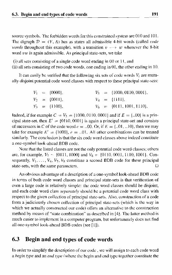
6.3. Begin and end types of code words 191

source symbols. The forbidden words for this constrained system are 0 I0 and 101.The digraph V = (V, A) has as states all admissible 4-bit words (caned codewords throughout this example), with a transition v ~ w whenever the 8-bitword vw is again admissible. As principal state-sets, we take

(i) all sets consisting of a single code word ending in 00 or 1 I, and(ii) all sets consisting of two code words, one ending in 01, the other ending in 10.

It can easily be verified that the following six sets of code words ~ are mutu­ally disjoint potential code word classes with respect to these principal state-sets:

Vj {OOOO},

V2 {001l},

V3 = {l100},

{1000, 0110, 0001},

{llll},

{Olll, 1001, 1110}.

Indeed, iffor example C = Vs = {l000, 0110, 0001} and if E = {..OO} is a prin­cipal state-set, then E' = {OlIO, 0001} is again a principal state-set and consistsof successors in C ofthe code worde = ..00. Or, if E = {..Ol, .. 10}, then we maytake for example E' = {lOOO}, e = ..0 I. All other combinations can be treatedsimilarly. The conclusion is that the six code word classes above indeed constitutea one-symbol look-ahead BDB code.

Note that the listed classes are not the only potential code word classes; othersare, for example, V7 = {Olll, lOOO} and Vs = {OlIO, 0001,1110, 1001}. Con­sequently, VI, ... , V4, V7 , Vs constitute a second BDB code for these principalstate-sets, with the same parameters. 0

An obvious advantage of a description of a one-symbol look-ahead BDB codein terms of both code word classes and principal state-sets is that verification ofeven a large code is relatively simple: the code word classes should be disjoint,and each code word class separately should be a potential code word class withrespect to the given collection of principal state-sets. Also, construction of a codefrom a judiciously chosen collection of principal state-sets (which is the way inwhich we actually constructed our code) offers an alternative to the constructionmethod by means of "state combination" as described in [4]. The latter method ismuch easier to implement in a computer program, but unfortunately does not findall one-symbol look-ahead BDB codes (see [1]).

6.3 Begin and end types of code words

In order to simplify the description of our code, we will assign to each code worda begin type and an end type (where the begin and end type together constitute the

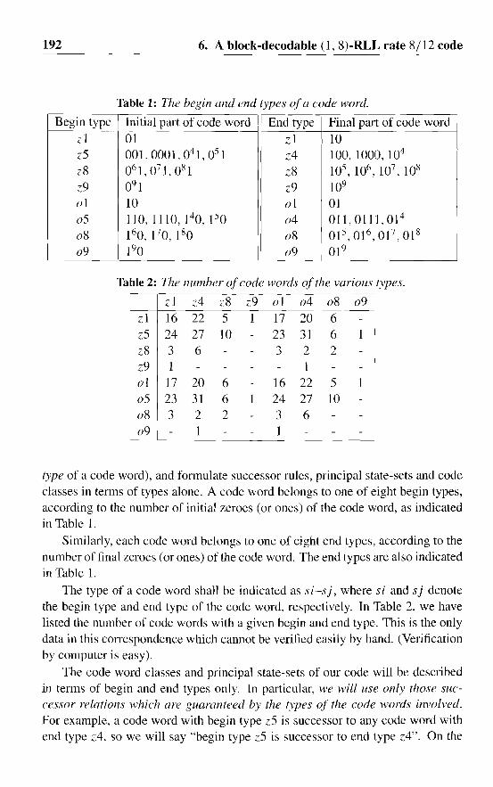
192 6. A block-decodable (l, 8)-RLL rate 8/12 code

Table 1: The begin and end types ofa code word.

Begin type I Initial part of code word End type Final part of code wordz1 01 z I 10z5 001,0001,04 1,05 1 z4 100,1000,104

Z8 06 1, 07 1, 08 1 Z8 105 , 106 , 107 , 108

z9 09 1 z9 109

01 10 01 0105 110,1110,1 40,1 50 04 011,0111,01 4

08 160,1 70,1 80 08 01 5,01 6,01 7 ,018

09 190 09 01 9

Table 2: The number ofcode words ofthe various types.---

zl z4 z8 z9 01 04 08091zl 16 22 5 1 17 20 6z5 24 27 10 23 31 6 1z8 3 6 3 2 2z9 1 101 17 20 6 16 22 5 105 23 31 6 24 27 1008 3 2 2 3 6

I~- 1 1 -

type of a code word), and formulate successor rules, principal state-sets and codeclasses in terms of types alone. A code word belongs to one of eight begin types,according to the number of initial zeroes (or ones) of the code word, as indicatedin Table 1.

Similarly, each code word belongs to one of eight end types, according to thenumber of final zeroes (or ones) of the code word. The end types are also indicatedin Table 1.

The type of a code word shall be indicated as si-sj, where s i and sj denotethe begin type and end type of the code word, respectively. In Table 2, we havelisted the number of code words with a given begin and end type. This is the onlydata in this correspondence which cannot be verified easily by hand. (Verificationby computer is easy).

The code word classes and principal state-sets of our code will be describedin terms of begin and end types only. In particular, we will use only those suc­cessor relations which are guaranteed by the types of the code words involved.For example. a code word with begin type z5 is successor to any code word withend type z4, so we will say "begin type z5 is successor to end type z4". On the

6.4. Description of the code

Table 3: Successor relations between end and begin types.

end type begin type successorszl 21 z5 28 - - - - -

24 21 25 - - - 05 08 09

z8 zl - - - - 05 08 09

z9 - - - - - 05 08 09

01 - - - - 01 05 08 -

04 - z5 z8 z9 01 05 - -

08 - z5 z8 z9 01 - - -

09 - ;::5 z8 z9 - - - -

193

other hand, begin type z5 is not successor to end type z8, although some particularcode word of that begin type such as 001 ... is a successor to a code word suchas ... 100000 of that end type. In Table 3 we have listed the various successorrelations according to type.

6.4 Description of the code

Our code consists of 256 disjoint code word classes. Each code word class isof a certain (code word class) type, where the type of a code word class is thecollection of types of its member code words. The principal state-sets of our codewill be described in terms of end states only; a set of code words is a principalstate-set if and only if the collection of end types of the code words constitute oneof the following six sets.

Fj = {z4}, F2 = {04}, F3 = {zl, ol},

F4 = {z8, 08}, Fs = {z8, 09}, F6 = {z9, 08}.

(Compare this to the description of the principal state-sets in Example 1.) Inwhat follows, when we use the expression "potential code word class", this willalways be understood to mean "with respect to the above collection of principalstate-sets". As a consequence of the above definition of the principal state-sets,the property of being a potential code word class depends only on type. (Recallour restriction on allowable successor relations as agreed in Section 3.) Let usconsider a few examples.

Example 2: The set {z5-z4} (representing a set that contains a single codeword, of type z5-z4) is a potential code word class type. Indeed, first we remarkthat {z4} = Fj is end type set of a principal state-set. Secondly, the begin type z5

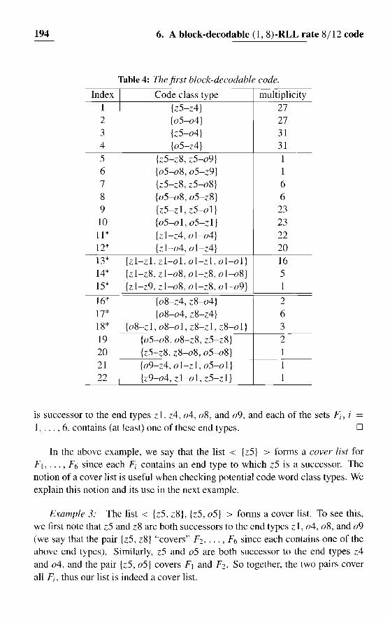
194 6. A block-decodable (1, 8)-RLL rate 8/12 code

Table 4: The first block-decodable code.

Index Code class type multiplicity

1 {z5-z4} 272 {05-04} 273 {z5-04} 314 {05-z4} 31

5 {z5-z8, z5-09} 16 {05-08,05-z9} 17 {z5-z8, z5-08} 68 {05-08,05-z8} 69 {z5-z1, z5-01} 2310 {05-01,05-z1} 23L1* {zl-z4,01-04} 2212* {zl-04,01-z4} 2013* {zl-zl,zl-01,01-zl,01-01} 1614* {zl-z8,zl-08,01-z8,01-08} 515* {zl-z9,zl-08,01-z8,01-09} 1

I

16* {08-z4,z8-04} 217* {08-04, z8-z4} 618* {08-z1,08-01,z8-z1,z8-01} 3

19 {05-08,08-z8,z5-z8} 220 {z5-z8,z8-08,05-08} 1

21 {09-z4,01-zl,05-01} 122 {z9-04,zl-01,z5-z1} L

is successor to the end types z 1, z4, 04, 08, and 09, and each of the sets F;, i =1, ... , 6, contains (at least) one of these end types. 0

In the above example, we say that the list < {z5} > forms a cover list forFl, ... , F6 since each F; contains an end type to which z5 is a successor. Thenotion of a cover list is useful when checking potential code word class types. Weexplain this notion and its use in the next example.

Exarnple 3: The list < {z5. z8}, {z5, 05} > forms a cover list. To see this,we first note that z5 and z8 are both successors to the end types Z1, 04, 08, and 09(we say that the pair {z5, z8} "covers" F2, ... , F6 since each contains one of theabove end types). Similarly, z5 and 05 are both successor to the end types z4and 04, and the pair {z5, 05} covers F1 and F2. So together, the two pairs coverall F;, thus our list is indeed a cover list.

6.5. Discussion

Table 5: Covering lists for the code in Table 4.

Index Covering lists1-10 < {z5} > and < {05} >11-15 < {zl}, {01} >16-18 < {z8}, {08} >19-20 < {05, 08}, {05, z5} > and < {z5, z8}, {z5, 05} >21-22 < {09}, {oj, 05} > and < {z9}, {zl, z5} >

Consequently, for example the set

{z5-z8,z8-09,z5-z1,05-01}

195

constitutes a potential code word class type, since each of the two sets of begintypes that make up the cover list are combined with sets of end types F;, herei = 5, 3. A second example is formed by the set

{z5-z8, z8-09, 05-08},

where the same cover list is now combined with the sets Fs and F4. D

Our description of the code will consist of a list containing the potential codeword class types, together with the number of code word classes of each type (Ta­ble 4). To ensure that the code word classes are indeed disjoint, the reader mustverify that enough code words of the various types are available, using Table 2.To help in checking the code word class types, we also list in Table 5 a coveringlist for each of the code word class types. Observe that since the collection ofprincipal state-sets is invariant under 0 -<--+ 1, the successor relations, and hencethe collection of potential code word classes, are invariant under z -<--+ o. In Ta­ble 4 symmetric types are marked with an asterisk. The code uses all availablecode words except for one of each of the three types z9-z1, 09-01, and z8-08.Therefore, we may, at the cost of one additional code word class type, obtain afully symmetric code by adding a code word with type z8-08 to one of the twocode word classes of the type with index 19 in Table 4.

This code is not the only BDB code with these parameters. A second code isgiven in Table 6, with covering lists as in Table 7. (The first 10 code class typesare identical to those of the first code, with the same multiplicities.)

6.5 Discussion

We have described two new rate 8/12 0,8) RLL block-decodable codes withblock size twelve, well adapted to byte-oriented storage systems since error prop­agation is limited to one byte. The codes allows a relatively simple description

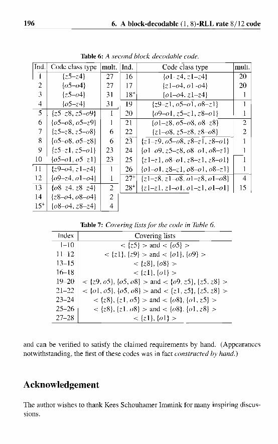
196 6. A block-decodable (1, 8)-RLL rate 8/12 code

Table 6: A second block-decodable code.

Ind. Code class type mult. Ind. Code class type mult.I {z5-z4 } 27 16 {01-z4, zl-z4} 202 {05-04} 27 17 {zl-04, 01-04} 203 {z5-04} 31 18* {01-04,zl-z4} 14 {05-z4} 31 19 {z9-z1, 05-01, 08-zI} 15 {z5-z8, z5-09} 1 20 {09-01,z5-z1,z8-01} 16 {05-08,05-z9} 1 21 {01-z8, 05-08, 08-z8} 27 {z5-z8, z5-08} 6 22 {zl-08,z5-z8,z8-08} 28 {05-08,05-z8} 6 23 {zl-z9,05-08,z8-z1,z8-oI} 19 {z5-zI, z5-01} 23 24 {oI-09, z5-z8, 08-01, 08-z1} 1

10 {05-oI,05-z1} 23 25 {zl-zl,08-01,z8-z1,z8-01} 111 {z9-04, zI-z4} 1 26 {01-oI,z8-z1,08-01,08-z1} 112 {09-z4,01-04} 1 27* {zl-z8,zl-08,01-z8,01-08} 413 {08-z4, z8-z4} 2 28* {zl-zl,zI-ol,ol-zl,ol-ol} 1514 {z8-04,08-04} 215* {08-04, z8-z4} 4

Table 7: Covering lists for the code in Table 6.

Index Covering lists< {z5} > and < {05} >

< {zl}, {z9} > and < {01}, {09} >< {z8}, {08} >< {zl}, {all >

< {z9, 05}, {05, 08} > and < {09, z5}, {z5, z8} >< {01, 05}, {05, 08} > and < {zl, z5}, {z5, z8} >

< {z8}, {zl, 05} > and < {08}, {ai, z5} >< {z8}, {zl, 08} > and < {08}, {oI. z8} >

< {zl}, {0I} >

1-1011-1213-1516-1819-2021-2223-24

25-261

27-28---------'--------'--'---'-------=------------

and can be verified to satisfy the claimed requirements by hand. (Appearancesnotwithstanding, the first of these codes was in fact constructed by hand.)

Acknowledgement

The author wishes to thank Kees Schouhamer Immink for many inspiring discus­SiOns.

References

References

197

[1] H.D.L. Hollmann, "Bounded-delay encodable, block-decodable codes forconstrained systems", IEEE Trans. Inform. Theory, vol. 42, no. 6, Nov.1996.

[2] H.D.L. Hollmann, "On the construction of bounded-delay encodable codesfor constrained systems", IEEE Trans. Inform. Theory, vol. 41, no. 5, pp.1354-1378, Sept. 1995.

[3] H.D.L. Hollmann, "On an approximate eigenvector associated with a mod­ulation code", to appear in IEEE Trans. h~form. Theory.

[4] K.A.S. Immink, "Block-decodable runlength-limited codes via look-aheadtechnique", Philips J. Res., vol. 46, no. 6, pp. 293-310, 1992.

[5] K.A. Schouhamer Immink, Coding techniques for digital recorders, Engle­wood Cliffs, NY: Prentice-Hall, 1991.

[6] R.L. Adler, D. Coppersmith, and M. Hassner, "Algorithms for sliding blockcodes. An application of symbolic dynamics to information theory", IEEETrans. Inform. Theory, vol. IT-29, no. 1, pp. 5-22, Jan. 1983.

[7] P.A. Franaszek, "Construction of bounded delay codes for discrete noiselesschannels", IBM J. Res. Develop., vol. 26, pp. 506-514, July 1982.

[8] A. Lempel and M. Cohn, "Lookahead coding for input-restricted channels",IEEE Trans. Inform. Theory, vol. IT-28, pp. 933-937, Nov. 1982.

[9] B. Marcus and R. Roth, "Bounds on the number of states in encoder graphsfor input-constrained channels", IEEE Trans. b~fonll. Theory, vol. IT-37, no.3, pp. 742-758, May 1991.

Chapter 7

On an approximate eigenvectorassociated with a modulationcode

Abstract - Let S be a constrained system of finite type, described in terms ofa labeled graph M of finite type. Furthermore, let C be an irreducible constrainedsystem of finite type, consisting of the collection of possible code sequences of somefinite-state encodable, sliding-block decodable modulation code for S. It is knownthat this code could then be obtained by state-splitting, using a suitable approximateeigenvector. In this paper, we show that the collection of all approximate eigenvectorsthat could be used in such a construction of C contains a unique minimal element.Moreover, we show how to construct its linear span from knowledge of M and Conly, thus providing a lower bound on the components of such vectors.

For illustration we discuss an example showing that sometimes arbitrary largeapproximate eigenvectors are required to obtain the best code (in terms of decoding­window size) although a small vector is also available.

Index Terms - Constrained systems, state-splitting, sliding-block decodable, ap­proximate eigenvector.

7.1 Introduction

Digital data storage systems commonly employ a modulation code to provide thedata as written on the storage medium with certain desirable properties. A well­known example is the use of (d, k) codes in magnetic storage systems to combatintersymbol interference and loss of clock. Typically, the collection of allowable

© 1996. IEEE. To appear in IEEE Transactions on Information Theory. Reprinted with per­miSSIOn.

200 7. On an approximate eigenvector

sequences (called the constrained system) can be described by means of a labeleddirected graph as the collection of all label sequences of paths in this graph.

In this paper, a modulation code for a constrained system consists of a finite­state encoder which maps arbitrary sequences of source symbols into allowablesequences, and a decoder capable of retrieving the original source sequence fromthe code sequence. The code system of a modulation code is the collection of allpossible code sequences of the code.

Since modulation codes are often used in a noisy environment. code sequencesget corrupted by noise, so will contain errors. It is therefore necessary to considerthe problem of error propagation. To limit error propagation, most practical codesare sliding-block decodable. Here, the decoder needs to base its decision on asource symbol only on the present code symbol together with a at most m previouscode symbols and at most a upcoming code symbols, for some numbers m and a.Evidently, one error in the code sequence thus propagates into at most m + I + a

errors in the source sequence. The number m + I + a is called the decodingwindow size of the code. This number is an important parameter of a code, relatedto the maximum error propagation and also to the amount of hardware needed toimplement the decoder, and should therefore be as small as possible.

Many code construction methods involve manipulation of the graph that de­scribes the constraint, under guidance of an approximate eigenvector, a collectionof non-negative integer weights associated with the vertices (states) of the graphwith the property that N times the weight of a state is at most equal to the sumof the weights of the successors of this state. Here N is a number related to thedesired rate of the code. A typical example of such methods is the state-splittingalgorithm as described in [1].

Recently [2], [3,4], this method has been shown to be universal, that is, es­sentially, each sliding-block decodable code for a constraint of finite type with acode system of finite type can be obtained by this method, with a proper choicefor the approximate eigenvector. (In fact, the results in [2] apply to all constrainedsystems, not just those of finite type; in more general situations some additionaloperations are required.) The extend of this result is discussed in Chapter V, Ap­pendix B, where some claims in [4] are further specified.

Generally speaking, distinct approximate eigenvectors lead to different codes.The usual approach is to choose such a vector with small components, since thisleads to the smallest currently known upper bound on the decoding window size.However, it is known [4] that such a choice does not always leads to the best code.We will present a sequence of examples where the smallest available vector hasmaximum component equal to two while the vector that leads to the best (block­decodable) code necessarily has maximum component at least N, for each choiceof N. (The smallest vector leads to a decoding window of two codewords.)

7.2. Notation and background 201

This paper has been written in an effort to clarify the intimate relation betweenapproximate eigenvectors on the one hand, and code systems of modulation codeson the other hand. Our approach is consistent with the Willems' approach [9] toinvestigate properties of a system based only on knowledge about the sequencesthat make up the system.

We will show that each irreducible finite-type code system of a sliding-blockdecodable code that is contained in a given constrained system of finite type and isobtained by the state-splitting algorithm determines a unique approximate eigen­vector, with the properties that (i) the code system can be constructed with thisvector, and (ii) each other vector that can be used to construct this code systemis at least as large (component-wise) as this vector. Unfortunately, in general weknow of no method to find this vector. However, we do present some methods toobtain its linear span, thus providing a lower bound on approximate eigenvectorsthat can construct the given code.

7.2 Notation and background

We begin by establishing our notation. For further details, we refer to [3].A constrained system is typically described in terms of a labeled directed

graph, which in this context is often referred to as a Finite-State Transition Di­agram or FSTD. Here, a FSTD M consists of a finite collection V of states anda finite collection A of labeled transitions. Each transition a of M has a labelL(a), an initial state beg(a) and a terminal state end(a), and is referred to as atransition from beg(a) to end(a) with label L(a). We denote by A v the collectionof transitions from state v, that is, all transitions a with beg(a) = v.

The constrained system S presented by M is the collection of all label se­quences L(al) ... L(a,,) of paths al ... an in M. (Here and in what follows,when we say "path" we always refer to a directed path.)

We say that the FSTD M is offinite type if there are numbers m and a suchthat, for each path a-Ill· .. ao· .. aa, transition ao is uniquely determined by thelabel sequence L(a-m )··· L(ao) ... L(aa) of the path. A constrained system issaid to be of finite type if it can be presented by a FSTD of finite type. (As iswell-known, this is the case precisely when the system can be described in termsof a finite collection of "forbidden subwords", see e.g. [I].) M is said to bedeterministic if in each state the transitions leaving that state carry distinct labels.

A (rate-N) encoder is a FSTD M in which a constant number of N transitionsleave each state, and that is lossless, i.e., any two distinct paths in M with the sameinitial state and terminal state generate distinct label sequences. In this paper,when we speak of a code, we always mean a code that has an encoder of this type.

202 7. On an approximate eigenvector

Mostly, we even require that the encoder is sliding-block decodable, i.e., that Mis of finite type.

A FSTD M is irreducible if for each pair of states (v, w) there is a pathin M from v to w. Also, a constrained system S is called irreducible if for eachtwo sequences x and y contained in S and each two indices nand m there ex­ists a sequence z in S and an integer k > 0 such that Zi = Xi for all i ::: nand Zn+k-m+i = Yi for all i ::: m. In other words, there exists a word WI ... Wk-I

such that the sequence

... Xn-IXnWI··· Wk-IYmYm+1 ...

is again contained in S. Note that a constrained system S presented by an irre­ducible FSTD M is irreducible. Conversely, an irreducible constrained system Spresented by an FSTD M is also presented by some irreducible component of M([6]). A component of M is called a sink if no transitions leave this component.Each FSTD M contains at least one irreducible sink.

With a FSTD M we associate its adjacency matrix DM, a IV I x IV I matrixfor which DM (v, w) counts the number of transitions from state v to state w. An[M, N]-approximate eigenvector cP consists of a collection of non-negative inte­ger weights cPv, not all zero, associated with the states v of M, with the propertythat N times the weight of a state v is at most equal to the sum of the weights ofterminal states of the transitions from state v, that is,

N cPv ::: L cPend(a)(lEA v

holds for each state v. The above condition is usually expressed as

(1)

(2)

where the inequality is to be interpreted component-wise.Next, we will give a very brief outline of state splitting. Further details can be

found, e.g., in [7] or [3]. A round ofstate-splitting is a method to transform a givenFSTD M into a new FSTD M', in the following way. For each state v of M, wepartition the set A v of transi tions leaving v into sets A ~, i = I, ... , n v. TheFSTD M' is then constructed as follows. Each state v of M produces states vi,i = I, ... , n v, in M', and each transition CY, from state v to state w, and containedin A~, say, produces transitions

j = I, ... , n w , in M', all of which inherit their codeword label from CY.

7.2. Notation and background 203

So each state v splits into a number of states Vi, where state vi representsthe part of v that can be left by transitions a in A~. Moreover, each transition asplits into transitions a j , where a j represents the part of a that leads to the j-thpart of the terminal state of a. We will refer to states vi and transitions a j aschildren of state v and transition a in M', and to v and a as their parents in M,respectively. We extend this notion of children and parents to paths in M and M'in the obvious way.

From the above description it is immediate that all children a' fJ' in M' ofa given path afJ in M agree in transition a'. ("A transition in M with a givenfuture determines a unique transition in M':') Thus, the parent/child relation infact provides a one-to-one correspondence between bi-infinite paths in M and M'and, in particular, M and M' generate the same constrained sequences.

We say that an FSTD M is transformed into the FSTD M* by k rounds ofstate-splitting if M* is the result of a sequence of transformations

where each intermediate transformation consists of a round of state-splitting.The parent/child relation extends in the obvious way to states, transitions, and

paths in M and M*. Moreover, it is easily seen that each state (transition) in M*has a unique parent state (transition) in M, and that all children a~ ... a; in M*of a given path ao ... ak in M agree in the first transition a~.

Now we come to the notion of ae-consistent state-splitting. This method infact transforms apair (M, ¢) consisting of an FSTD M and an [M, N]-approx­imate eigenvector ¢. We say that a round of state-splitting that transforms Minto M' as explained earlier is ae-consistent (with respect to the approximate ei­genvector ¢) if, for each state v of M, the weight ¢v associated with v can be dis­tributed over its children vi in M' in such a way that the resulting assignment ¢'of weights to the states of M' now constitutes an [M', N]-approximate eigenvec­tor. Similarly, we say that the pair (M, ¢) is transformed into the pair (M*, ¢*)by k rounds ofae-consistent state-~plitting if the pair (M*, ¢*) is the result of krounds of ae-consistent state-splitting. In this situation, we say that M* is ob­tained from M by ae-consistent state-splitting (with respect to the approximateeigenvector ¢).

The importance of the notion of ae-consistent state-splitting follows from thefollowing observation: if the weights of all the states of an irreducible sink of M *are equal, then by the definition of an approximate eigenvector the out-degree ineach of these states is at least N, so that from M * we can obtain an encoder for theconstrained system S presented by M. In [1] the authors describe an algorithm,the ACH state-splitting algorithm, which demonstrates that for each approximate

204 7. On an approximate eigenvector-----------

eigenvector there exists a sequence of ae-consistent state-splittings leading in theabove way to an encoder.

It is almost, but not quite true that each finite-state encodable, sliding-blockdecodable code for a finite-type constraint can be obtained in this way (one furtheroperation called "state-expansion", duplication of states, is required in the casewhere the encoder graph is not of finite type, see [2]). It is true, though, that, givena sliding-block decodable finite-state encodable code, a code can be obtained bystate-splitting that has the same code system as the given code and that can bedecoded by the same sliding-block decoder. We refer to [2], [3,4], and Chapter 5for further details.

7.3 Preliminaries

We begin with a simple but important observation. Suppose that the FSTD Nis obtained from M by state-splitting, followed by the deletion of certain statesand transitions, and suppose furthermore that each state of N has out-degree atleast N. For each state v of M. let Yv denote the number of its children in N.

Proposition I: The vector y is an [M. N]-approximate eigenvector, and thestate-splitting steps are ae-consistent with respect to y.

Proof In each intermediate FSTD M(i), we can take as the weight of a stateits number of children in N. That this is indeed an approximate eigenvectorfor M(i) can be shown directly by induction on i = k. k - 1, ... ,0, but fol­lows also from Theorem 4 below applied to M(i) instead of M. Further detailsare left to the reader. 0

In the remainder of this paper, we will make the following assumptions. Weare given a constrained system S, presented by an irreducible FSTD M of finitetype with memory m and anticipation a, and an [M. N]-approximate eigenvec­tor ¢. The FSTD M* is obtained from the pair (M, ¢) by k - I rounds of ae­consistent state splitting with respect to ¢. The FSTD N is obtained from M* bydeleting certain vertices and transitions. We assume thatN is irreducible, and thatexactly N transitions leave each state ofN (so N is an encoder graph). Moreover,we assume that all vertices of./I[ carry the same non-zero weight in M*. Note thatthis includes the case where all vertices carry the same non-zero weigth in .M; inthat case, our assumptions comply with the scenario when N is obtained from Mand ¢ by ae-consistent state-splitting. We will refer to the constrained systemC S; S generated by N as the code system. Note that the encoder N will againbe of finite type, and hence the code system C generated by N is the code system

7.4. The number of children in N of paths in M 205

of a sliding-block decodable code. The adjacency matrices of M and N will bedenoted by DM and DN, respectively.

A state v in M will have n v children vi, 1 ::'S i ::'S n l " in M*, of which thestates vi, i E Iv, are contained in N. The number 1 Iv 1 of children of state v in Nwill be denoted by Yv. (Note that Yv ::'S cPv.) Similarly, a transition a in M willhave no: children a J, 1 ::'S j ::'S no:, in M*.

The collection of paths in M of length n starting in state v or starting withtransition a, and having a child in N, will be denoted by i;~n) or i;[yn) , respectively.Moreover, for n ~ k we let i;~7) and i;~~)denote the subsets of i;~n) and i;[yn) con­

sisting of those paths whose child (or children) in N start in state vi or start withtransition a J, respectively. Note that the first k transitions of a path in M uniquelydetermine the first transition of any of its children in M*, that is, for n ~ k thesets i;~7), 1 ::'S i ::'S Ill" partition i;~n) and the sets i;~~), 1 ::'S j ::'S no:, partition

i;[yn). This observation will be used repeatedly in what follows.

Our aim will be to find a lower bound on cP using only knowledge about Mand C. Note that M and C together determine the number N.

7.4 The number of children in N of paths in M

Our aim in this section will be to derive an expression for the number 1 i;~n) 1 ofpaths of length n in M starting in state v that have a child in N, and to study itsbehavior if n ---+ 00. In order to do so, we will need the following result on theasymptotic behavior of powers of the adjacency matrix DN of N.

Proposition 2: We have that

where 1 denotes the all-one vector and b denotes the (unique) positive left-eigen­vector of DN with corresponding eigenvalue N for which bTl = 1.

Proof Our assumptions on N imply that DN is irreducible, non-negative,and has right-eigenvector 1 with eigenvalue N. Now the existence of b and theasymptotic result in the theorem follow from standard Perron-Frobenius theory,see e.g. [8]. D

Next, for each state v* of N and each integer II ~ k, we define

(n) I - (n)Pv* = b v* I, (3)

206 7. On an approximate eigenvector

the number of paths of length n in M that have a child in N staI1ing in state v*.We observed earlier that for n ~ k, the sets 'E~7), i E Iv, partition 'E~"). hence

1'E~n)1 = L p;?iEI

"

Let p(lI) denote the vector with components p~~).

Proposition 3: The vectors p(Il), n ~ k. satisfy

p(n+l) = D.v p(n).

(4)

Proof For n ~ k, we have that

(n+1)Pv* 1'E~~+1)1

L 1'E~~+1)1ex*

" - (n)L..J ILend(ex*) I,ex*

where the sums are over all a* for which beg(a*) = v*.

Now, for each state v of M, we define

D

(5)

and we let e(n) denote the vector with components the eSn

). We will use the aboveresults to derive the following.

Theorem 4: (i) The vectors e(n), n = 1,2, ... , satisfy

Ne(n) :::: DMe(n-1).

(ii) For each state v, the limit

e v = lim e~n)n~oo

exists, and there is a constant c > 0 such that e= cy holds, where eis the vectorwith components ev .

Proof (i) To prove (i), it is sufficient to note that

I'E~n) I L I'E~z) Iex

< L I'E~~d(~) I,ex

7.5. How M and C determine e 207

where the sums are over all transitions a of M with beg(a) = v. The inequalityreflects the observation that there could be paths aj a2 ... an from v that are notin 't~n) but for which a2 ... an has a child in N; the set 't~n) can even be empty.

(ii) From Proposition 3, we may conclude that

for n ::: k. Hence by Proposition 2, we have that

lim N-npen) = N-k(bT . p(k»l.n~oc'

Putc = N-k(bT . p(k».

Note that c > O. From (4), we now conclude that

lim e(n)n----+oo v

D

Let e be the smallest non-negative non-zero integral vector in the linear spanof the vector e, or, equivalently, in the linear span of y. Then the above theoremhas the following consequence.

Theorem 5: Both y and e are [M, N]-approximate eigenvectors, and

¢:::y:::e.

Proof Since both y and e are integral and contained in the linear span of e,the fact that both vectors are approximate eigenvectors follows from Theorem 4.From the definition of e, the inequality y ::: e is obvious. Finally, the numberof children Yv of a state v of M in N is certainly not greater than the number ofchildren of v in M*, which in turn is at most equal to ¢v if ¢v > 0; if ¢v = 0,then Yv = 0 by our assumption on N. D

7.5 How M and C determine eIn this section we will derive an expression for I't{:l) I in terms of M and thecodeword sequences C generated by N only. In view of Theorem 5, we thusobtain a lower bound for ¢ in terms of M and C alone. The result that we need isgiven by our next theorem.

208 7. On an approximate eigenvector

Theorem 6: The following statements are equivalent.(i) The path 0'00') ... O'n-I is contained in i;~n).

(ii) There exists a word x = X-m ... Xo' .. Xn+a-I in C that is generated in M bya path W = W- m ... Wn+a-I for which Wi = O'i, 0.::: i .::: n - 1.

P oF F' I ~ (n) . h h'ld * * . Nroo): Irst, et 0'00'1 ... O'n-I E L...v ,WIt c 1 0'0' .. a n - l III , say.Since N is irreducible, this path can be extended to a path a"'-m ... a~+a_l in N,with parent a-m ... ao· .. an-I' .. an+a-I in M. So if x is the word generated bythese paths, then x has the property in (ii).

Now suppose that x is a word in C as in (ii). Since x is in C, there is a pathfJ* = fJ"'-m'" fJ~+a-1 in N that generates x. Let fJ = fJ-m ... fJn+a-l denotethe parent in M of this path. By our assumption that M has memory m andanticipation a, the paths fJ and W agree in positions 0, ... , n - I, that is, fJi =

Wi = ai, 0 .::: i .::: n - 1, hence aOa) ... an-I has child fJ~'" fJ~-1 in N and is

contained in i;~n). D

The above theorem thus shows that i;~n), and hence e, is determined by Mand C only, and therefore does not depend on the particular encoder N.

7.6 Main results

We can now summarize the main results in this paper as follows.

Theorem 7: Let M be an FSTD of finite type, and let <P be an [M, N]­approximate eigenvector. Let C be an irreducible code system generated by someirreducible rate-N encoder FSTD N obtained from M and <P by ae-consistentstate splitting, and let ebe determined by M and C as in Theorem 6. Let Yv bethe number of children in N of state v in M. Then the fo11owing holds.(i) The encoder N can also be obtained by ae-consistent state-splitting from Mand y.

(ii) The inequality <Pv ::: Yv holds for each state v of M.(iii) The vectors eand yare linearly dependent.(iv) If e denotes the smallest non-zero non-negative integral vector in the linearspan of e(or, equivalently, in the linear span of y), then <Pv ::: ev holds for eachstate v of M.

This theorem has an important consequence.

Theorem 8: Let S be a constrained system of finite type, presented by anFSTD M of finite type, and let C be an irreducible code system of some en­coder obtained from an [M, N]-approximate eigenvector by ae-consistent state­splitting. (Here the value of N is determined by M and C.) Then there exists a

7.7. Some remarks 209

(unique) vector y* = y*(M, C) with the following properties.(i) The vector y* is an [M, N]-approximate eigenvector, and has the further prop­erty that C is the code system of a rate-N encoder that can be constructed by ae­consistent state-splitting from M and y*.(ii) Any other [M, N]-approximate eigenvector cP with this property satisfiescP ~ y*, that is, cPv ~ y: holds for each state v of M.

Proof Since the vector eas defined in Theorem 7 only depends on M and C,but not on the particular encoder N, it follows from part (iii) of Theorem 7 thatall the vectors y that can be obtained from encoders as described in that theoremare scalar multiples of the same vector e. Let y * = y *(M, C) be the smallest ofall such vectors y. (This minimum exists since all y have integer components.)Our two claims now follow from parts (i) and (ii) of Theorem 7. D

The above justifies to call this vector y* the approximate eigenvector of thecode system C. Unfortunately, the definition of y* is highly non-constructive.However, we can determine the linear span of y*, for example from an encoder Nfor C together with the state-splitting procedure used to obtain it and inspectionof the corresponding vector y. But the definition of y* gives no further clueson how y* itself could be found. It would therefore be interesting to obtain aconstructive description of y*, purely in terms of the sequences contained in C.Perhaps the methods in [2] can be of use to obtain such a result. Note also that thelower bounds on the number of encoder states derived in [6] deliver also a lowerbound on Lv y:, but in general the number of states in N can be reduced by statemerging and therefore such a bound need not be tight.

7.7 Some remarks

1. Provided that the constraint is of finite type, the approximate eigenvector ecan also be obtained in a different way. Let us define ~~n) to denote the numberof paths of length n in M that start in state v and generate a word in the codesystem C, and let

e~n) = I~~n) 1/N n.

If e(n) is the vector with components the numbers e~n), then we can show, by thesame method as used in Section 7.4, that the limit

e = lim e(n)11-----*00

exists and that e is again a scalar multiple of the vector y. We leave the verificationof these claims to the reader.

210 7. On an approximate eigenvector

2. Severall possible converses of Theorem 7 are certainly false. Firstly, itmay happen that a code system cannot be obtained by ae-consistent state splittingfrom an approximate eigenvector ¢ although ¢ :::: y = e holds (e.g., Exam­ple 3). Secondly, it is also possible that C cannot be obtained by ae-consistentstate-splitting from e (e.g., Example 2). And thirdly, there are examples of codesthat can be obtained by ae-consistent state splitting from distinct approximate ei­genvectors (e.g., Example 2). Let us say that an approximate eigenvector ¢ istight if none of the vectors ¢! obtained from ¢ by lowering some component byone is again approximate eigenvector. Perhaps it is true that independent tightapproximate eigenvectors always produce distinct code systems.

7.8 Applications

We will use our previous results to show that certain "good" codes can be ob­tained by ae-consistent state-splitting only with an approximate eigenvector con­taining "large" components. The main problem of code construction with theae-consistent state-splitting algorithm is the enormous amount of freedom, bothin the choice of state-splitting steps and labelling with source symbols, and in thechoice of an approximate eigenvector. Given an approximate eigenvector, someheuristics have been developed [7], [3] to guide the choice of the state-splittingsteps in order to obtain "good" codes. Also, both practical and theoretical con­siderations seem to suggest to choose an approximate eigenvector that is "small"and, in particular, to choose one with smallest maximal component. The follow­ing example shows in a rather strong sense that such a choice does not always leadto the best code available. Indeed, for each N :::: 3, we will construct a constrainedsystem of finite type SN, of capacity at least N, for which an approximate eigen­vector can be found with maximal component equal to two. We will show thateach SN affords a one-symbol encodable, block-decodable code CN, but that CNcan only be constructed by ae-consistent state-splitting with an approximate ei­genvector whose maximal component is at least N. In fact, we will shown thatno BDB code [4] can be found by ae-consistent state-splitting with an approxi­mate eigenvector whose maximal component is less than N. Here, a BDB codeessentially is a block-decodable code that can be encoded by a finite-state encoderwith a finite, bounded encoding delay. In this context, the labels of M are oftenrefened to a codewords. The collection of labels that decode to a fixed sourcesymbol is called a codeword class.

Example]: Let N be a fixed integer with N :::: 3, and let n = LN j2J. Weconsider the constrained system S with alphabet F = {I, 2, ... , N + I} and for­bidden words

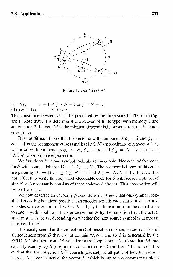
7.8. Applications

2

N

N + 1

Figure 1: The FSTD M.

N

N + 1

211

(i) Nj, n+l:::j:::N-1orj=N+1,

(ii) (N + l)j, I ::: j ::: n.

This constrained system S can be presented by the three-state FSTD M in Fig­ure 1. Note that M is deterministic, and even of finite type, with memory 1 andanticipation O. In fact, M is the minimal deterministic presentation, the Shannoncover, of S.

It is not difficult to see that the vector cP with components cPu = 2 and cPrlO =cPr!! = 1 is the (component-wise) smallest [M, N]-approximate eigenvector. Thevector cP' with components cP~ = N, cP~o = n, and cP~! = N - n is also an[M, N]-approximate eigenvector.

We first describe a one-symbol look-ahead encodab1e, block-decodable codefor S with source alphabet B = {I, 2, ... , N}. The codeword classes of this codeare given by F i = {i}, 1 ::: i ::: N - I, and FN = {N, N + I}. In fact, it isnot difficult to verify that any block-decodable code for S with source alphabet ofsize N ::: 3 necessarily consists of these codeword classes. This observation willbe used later on.

We now describe an encoding procedure which shows that one-symbol look­ahead encoding is indeed possible. An encoder for this code starts in state (J andencodes source symbol i, 1 ::: i ::: N - 1, by the transition from the actual stateto state (J with label i and the source symbol N by the transition from the actualstate to state 110 or 11 I, depending on whether the next source symbol is at most nor larger than n.

It is easily seen that the collection C of possible code sequences consists ofall sequences from S that do not contain "NN", and so C is generated by theFSTD M' obtained from M by deleting the loop at state N. (Note that M' hascapacity exactly log N.) From this description of C and from Theorem 6, it isevident that the collection i;~n) consists precisely of all paths of length n from vin M'. As a consequence, the vector cP', which is (up to a constant) the unique

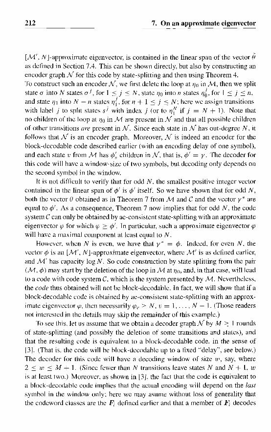
212 7. On an approximate eigenvector

[M', N]-approximate eigenvector, is contained in the linear span of the vector eas defined in Section 7.4. This can be shown directly, but also by constructing anencoder graph N for this code by state-splitting and then using Theorem 4.To construct such an encoder ./V, we first delete the loop at rio in M, then we splitstate () into N states () i , for I :::. j ::: N, state rio into n states 176, for 1 ::: j ::: n,and staterJ 1 into N - n states rJi ' for n + 1 ::: j ::: N; here we assign transitionswith label j to split states si with index j (or to 17f if j = N + 1). Note thatno children of the loop at rio in M are present in N and that all possible childrenof other transitions are present in N. Since each state in N has out-degree N, itfollows that N is an encoder graph. Moreover, N is indeed an encoder for theblock-decodable code described earlier (with an encoding delay of one symbol),and each state v from M has ¢~ children in N, that is, ¢' = y. The decoder forthis code will have a window-size of two symbols, but decoding only depends onthe second symbol in the window.

It is not difficult to verify that for odd N, the smallest positive integer vectorcontained in the linear span of ¢' is ¢' itself. So we have shown that for odd N,both the vector e obtained as in Theorem 7 from M and C and the vector y* areequal to ¢'. As a consequence, Theorem 7 now implies that for odd N, the codesystem C can only be obtained by ae-consistent state-splitting with an approximateeigenvector cp for which cp ~ ¢', In particular, such a approximate eigenvector cpwill have a maximal component at least equal to N.

However, when N is even, we have that y* = ¢. Indeed, for even N, thevector ¢ is an [M', N]-approximate eigenvector, where M' is as defined earlier,and M' has capacity log N. So code construction by state splitting from the pair(M, ¢) may start by the deletion of the loop in M at 170, and, in that case, will leadto a code with code system C, which is the system presented by M. Nevertheless,the code thus obtained will not be block-decodable. In fact, we will show that if ablock-decodable code is obtained by ae-consistent state-splitting with an approx­imate eigenvector cp, then necessarily CPv ~ N, v = 1, ... , N - 1. (Those readersnot interested in the details may skip the remainder of this example.)

To see this, let us assume that we obtain a decoder graph N by M ~ 1 roundsof state-splitting (and possibly the deletion of some transitions and states), andthat the resulting code is equivalent to a block-decodable code, in the sense of[3]. (That is, the code will be block-decodable up to a fixed "delay", see below.)The decoder for this code will have a decoding window of size w, say. where2 ::: w ::: M + 1. (Since fewer than N transitions leave states Nand N + 1, wis at least two.) Moreover, as shown in [3], the fact that the code is equivalent toa block-decodable code implies that the actual encoding will depend on the lastsymbol in the window only; here we may asume without loss of generality thatthe codeword classes are the Fi defined earlier and that a member of F i decodes

7.9. Discussion 213

as the source symbol i.We claim that such a code cannot exist if state a has less than N children

in N. This can be seen as follows. Fix i, 1 :::: i :::: N - 1. First note that theremust be a child of state a in N, say state aI, and a child of the loop a with labeli at state a in M, say aI, such that a 1 is a loop at a 1 in N. Indeed, the sourcesequence

... i, i, i, ...

is necessarily encoded by a path in N that (with the possible exception of thefirst transition) consists of children of transition a only, and therefore the patheventually consists of the repetition of a single loop in N.

Now, consider the encoding of a source sequence of the form

... i,i,i,k,k,k, ... , (6)

where 1 :::: k :::: N. After encoding of the last source symbol i, the encoder willbe in state a I. Then the next source symbol k will be encoded by a transitionin N that carries source label k and (codeword) label v, say. Hence the decodingwindow of the (w - 2)-but-last source symbol i looks like

i, i, ... , i, v.

By our earlier remark, this window decodes as v (or as N if v = N + 1) andshould decode as i, therefore v = i, so the transition that encodes k is also a childofa.

Now, if state a has fewer than N children in N, then the transition a can haveat most N - 1 children in N, hence some source symbol k does not occur assource label on any of these children, and, by the above reasoning, for this k thesource sequence (6) cannot be encoded properly. D

7.9 Discussion

There has always existed an intimate relation ~etween code construction methodson the one hand and approximate eigenvectors on the other hand. In an attempt toexplain some of the reasons for this connection, we have investigated the relationbetween a modulation code for a given constrained system and the approximateeigenvector used in ae-consistent state-splitting to construct the code.

In the case that the constraint is of finite type, our main result is a lowerbound on this approximate eigenvector, determined by the code sequences (thecode system) of the code only. It seems possible to derive a similar result in

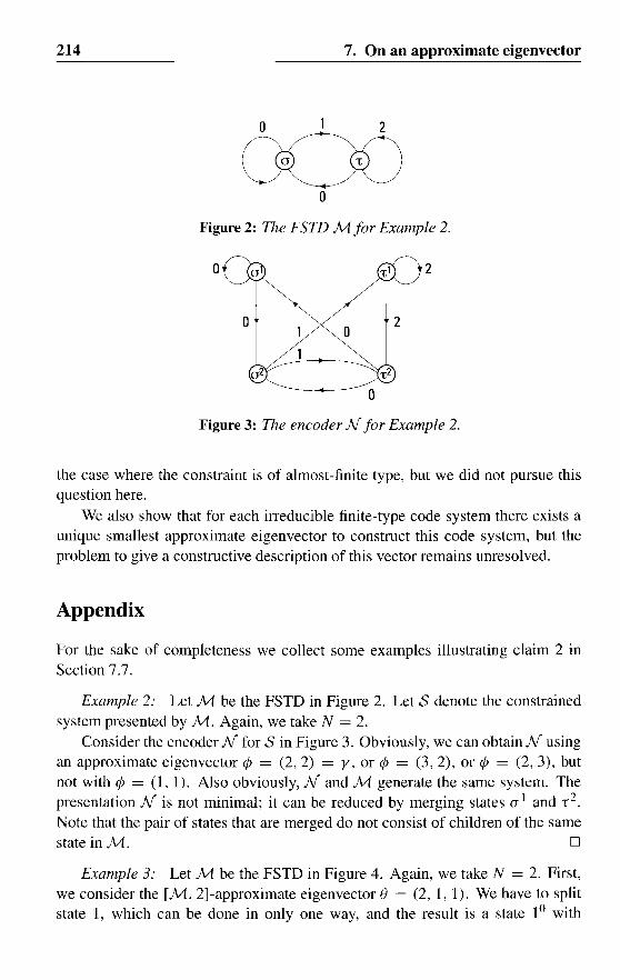
214

o

7. On an approximate eigenvector

2

o

Figure 2: The FSTD M for Example 2.

o

o

a

o 2

2

oFigure 3: The encoder N for Example 2.

the case where the constraint is of almost-finite type, but we did not pursue thisquestion here.

We also show that for each irreducible finite-type code system there exists aunique smallest approximate eigenvector to construct this code system, but theproblem to give a constructive description of this vector remains unresolved.

Appendix

For the sake of completeness we collect some examples illustrating claim 2 inSection 7.7.

Example 2: Let M be the FSTD in Figure 2. Let S denote the constrainedsystem presented by M. Again, we take N = 2.

Consider the encoder N for S in Figure 3. Obviously, we can obtain N usingan approximate eigenvector ¢ = (2, 2) = y, or ¢ = (3, 2), or ¢ = (2, 3), butnot with ¢ = (1,1). Also obviously, Nand M generate the same system. Thepresentation N is not minimal; it can be reduced by merging states u! and r 2.

Note that the pair of states that are merged do not consist of children of the samestate in M. D

Example 3: Let M be the FSTD in Figure 4. Again, we take N = 2. First,we consider the [M, 2]-approximate eigenvector e = (2,1,1). We have to splitstate 1, which can be done in only one way, and the result is a state 10 with

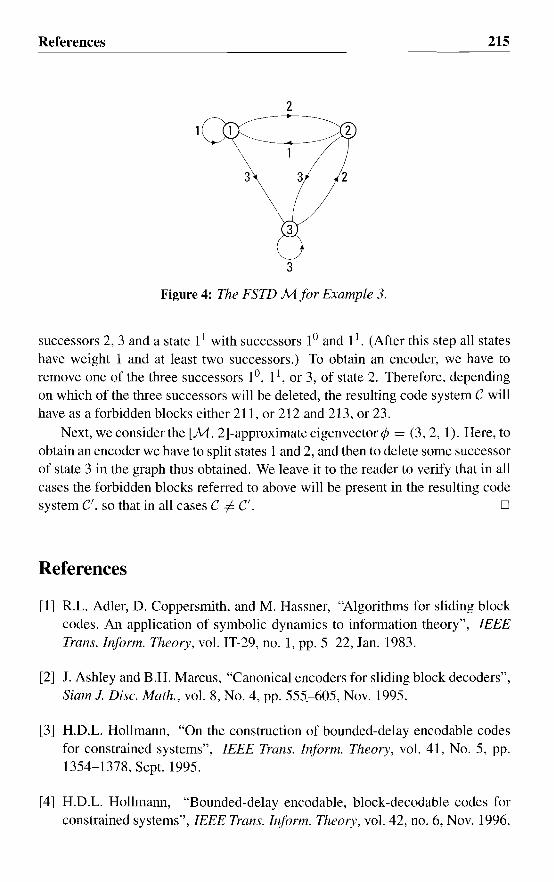
References

2

215

3

2

3

Figure 4: The FSTD M for Example 3.

successors 2, 3 and a state 11 with successors 10 and 11. (After this step all stateshave weight 1 and at least two successors.) To obtain an encoder, we have toremove one of the three successors 10, 11, or 3, of state 2. Therefore, dependingon which of the three successors will be deleted, the resulting code system C willhave as a forbidden blocks either 211, or 212 and 213, or 23.

Next, we consider the [M. 2]-approximateeigenvector¢ = (3,2,1). Here, toobtain an encoder we have to split states 1 and 2, and then to delete some successorof state 3 in the graph thus obtained. We leave it to the reader to verify that in allcases the forbidden blocks referred to above will be present in the resulting codesystem C', so that in all cases C :f- C'. D

References

[1] R.L. Adler, D. Coppersmith, and M. Hassner, "Algorithms for sliding blockcodes. An application of symbolic dynamics to information theory", IEEETrans. Inform. Theory, vol. IT-29, no. 1, pp. 5-22, Jan. 1983.

[2] J. Ashley and B.H. Marcus, "Canonical encoders for sliding block decoders",Siam J. Disc. Math., vol. 8, No.4, pp. 555.-605, Nov. 1995.

[3] H.D.L. Hollmann, "On the construction of bounded-delay encodable codesfor constrained systems", IEEE Trans. Inform. Theory, vol. 41, No.5, pp.L354-1378, Sept. 1995.

[4] H.D.L. Hollmann, "Bounded-delay encodable, block-decodable codes forconstrained systems", IEEE Trans. Inform. Theory, vol. 42, no. 6, Nov. 1996.

216 References

[5] H.D.L. Hollmann, "A block-decodable (d, k) = 0,8) runlength-limited rate8/12 code", IEEE Trans. Inform. Theory, vol. 40, No.4, pp. 1292-1296, July1994.

[6] B.H. Marcus and R. Roth, "Bounds on the number of states in encoder graphsfor input-constrained channels", IEEE Trans. Inform. Theory, vol. IT-37,no. 3, pp. 742-758, May 1991.

[7] B.H Marcus, PH. Siegel, and J.K. Wolf, "Finite-state modulation codes fordata storage", IEEE 1. Sel. Areas Commun., vol. 10, no. 1, pp. 5-37, Jan.1992.

[8] E. Seneta, Nonnegative matrices and Markov chains, New York: Springer,1981.

[9] J.e. Willems, "Models of dynamics", in Dynamics Reported, vol. 2, pp.171-266, New York: Wiley, 1989.

Summary

Modulation codes

This thesis concerns digital modulation codes or channel codes as employedin digital transmission or storage systems (e.g., a compact disc system). The dataprocessing in such systems can be sketched as follows. At the senders side, theanalogue data stream at the input (e.g., sound captured by a microphone) is firstsampled and digitized. Then the digital data thus obtained is compressed. Next,the compressed data is protected by means of an error-correcting code. Finally,the resulting digital data is transformed by means of a modulation code into a datasequence that possesses certain desirable properties, referred to as an admissiblesequence, which is subsequently transmitted or stored on a medium such as diskor tape, in analogue form (e.g., written on a compact disk).

At the receiver's side, the whole process is reversed. First the original digitalform of the transmitted or stored data is recovered as well as possible from theanalogue data that is received or read, and is transformed back by means of themodulation code. Then the error-correcting code is used to correct possibly cor­rupted parts of the data. Finally, the corrected data is decompressed and restoredto its original analogue form.

In the theory of modulation codes the following topics play an important role:kinds of collections of admissible sequences; construction of encoders that re­alise the transformation from arbitrary sequences to admissible sequences and thecorresponding decoders to recover the original sequences from their transformedform; the complexity and other aspects of encoders and decoders; and code effi­ciency.

As said above, modulation codes are employed to transform arbitrary datasequences into special, admissible sequences. Which sequences are admissibledepends on various technical constraints imposed by the system for which thecode is designed. Well-known examples that also playa role in this thesis arethe "dc-balanced" sequences, bipolar ({-I, l}-valued) sequences whose runningdigital sum does not surpass certain specified values (as a consequence, such se-

218 Summary-----------------------------

quences have a spectral zero at the null-frequency, "at dc"); the (d, k)-constrainedsequences, binary sequences in which each two consecutive symbols "1" are sep­arated by at least d and at most k symbols "0"; and the related class of (d, k)RLL sequences, binary sequences in which each group of successive symbols "0"or "1" in the sequence has size at least d + 1 and at most k + 1. (The practicalrelevance of such constraints is explained in the first chapter of this thesis.)

In all important applications, the collection of admissible sequences can beconveniently described as the collection oflabel sequences generated by the walksin a certain labeled directed finite graph. (Think of such a graph as of a descriptionof the crossings and their connecting roads of a town where only one-way trafficis allowed. The labels are the street-names; the admissible sequences are all thosesequences of street-names that correspond to possible tours in the town.)

The graph describing a given collection of admissible sequences is not unique,and in fact many code construction methods for modulation codes (i.e., of en­coders and decoders) essentially depend on finding a suitable graph to describethe given collection of sequences.

An important type of constraint often encountered in applications is that nomember from a given finite set of patterns is allowed to occur in a transmitted se­quence. (For example, it is not difficult to see that the (d, k) constraint mentionedearlier is of this type.) A collection of sequences that satisfy such a "constraint offinite type" always admits a description by means of a suitable graph.

Obviously, there are more arbitrary sequences of a certain length than admis­sible sequences of that length. This simple observation has as important con­sequence that encoding in general will necessarily result in a longer admissiblesequence: more bits will be required to represent the information. The averageratio of the length of the original sequence to the length of the corresponding en­coded sequence is called the "rate" of the code. For example, if encoding doublesthe length, then the rate equals 1/2. COne bit of information per two encodedbits".) The rate of a code is always a number between zero and one.

In general we can say, "the higher the rate the better". However, it turns outthat for each collection of admissible sequences that can be described by meansof a graph, there actually is a limit to the achievable rate. This maximal rateis called the capacity of the collection of admissible sequences. The capacitycan be computed relatively straightforward from a given graph description. Theefficiency of a code is the ratio of the rate of the code to the capacity.

Generally speaking, the received sequence to be decoded will not be exactlythe same as the originally transmitted sequence, due to, e.g., possible damage tothe storage medium (scratches on the disk) in the case of data storage, or badweather conditions (lightning) in the case of data transmission. In other words,the received sequence may contain errors. The decoder will have to be able to

Summary 219

deal with these errors: we cannot allow the situation where a single erroneous bitcan cause the decoder to produce an enormous amount of errors in the originalsequence. (The effect that a single error may lead to several errors after decodingis called error propagation.)

For this reason, most practical decoders employ a decoding window of a fixedsize. Here, to recover a specific original bit, only a part of the received sequenceis involved, namely only the part that falls within the decoding window of this bit.We can now imagine the decoding process as a sequence of decoding decisions,where we slide the decoding window over the sequence that is to be decoded.This explains the pictorial name "sliding-block decoder" in use for this type ofdecoder. Note that an error in the received sequence only influences the decodingdecision as long as it is contained in the decoding window, hence indeed affectsonly a limited number of the recovered bits.

The size of the decoding window is an important parameter of a code: not onlydoes this size provide an upper bound to the expected amount of error propagation,it also gives an indication of the complexity (and hence of the size of a hardwareimplementation) of the decoder.

A special case of these sliding-block decodable codes is constituted by theblock-decodable codes. These codes can be decoded by first grouping the receivedbits into blocks of a fixed size, followed by separate decoding of each of theblocks, independent of preceding and succeeding blocks.

In Chapter 1 we first give an overview of the different parts that constitute adigital communication scheme. Here, we emphasize the mathematical principlesthat underly the functioning of these parts and their interaction with various prac­tical constraints. Then we present an extensive overview of the various aspects ofthe theory of modulation codes, as well as an extensive discussion of and moti­vation for the further material in this thesis. All the topics mentioned above arereviewed again in more detail, on a somewhat deeper level but as far as possiblein an elementary way. With an exception here and there, this chapter consists ofknown material.

In Chapter 2 we compare two modulation codes for the dc-balanced con­straint, namely the "polarity-bit" code, and a code introduced by Knuth. It hadbeen shown earlier that the "sum variance" of such codes constitutes a good per­formance criterium. My contribution here is an exact evaluation of a good ap­proximation to the sum variance of the Knuth code, which required the solutionof a combinatorial counting problem. The results show that the performance ofthis code in general does not justify its greater complexity.

In many applications, the encoded data is grouped into large blocks of a fixedsize called "frames". Here, the beginning of each frame is marked by a fixedsynchronization pattern that is not allowed to occur anywhere else in the data

220 Summary

stream. This requirement leads to a certain loss of capacity. In Chapter 3 wedescribe a method to compute this loss of capacity for each given pattern whenmoreover the encoded data has to obey a (d, k) constraint. My contribution heremainly concerns the employed enumerative techniques.

The next three chapters are concerned with BO codes, sliding-block decodablecodes for constraints of finite type that can be encoded with a bounded encodingdelay (or, equivalently, by looking ahead at a limited number of bits).

One of the most important code construction methods is the ACH state-split­ting algorithm. This method acts directly on a graph that presents the constraint;in a number of rounds of state-splitting, this graph is guaranteed to be transformedinto an encoder for the constraint. This process is guided by an "approximate ei­genvector", certain integer weights associated with the vertices ("states") of thegraph. In general, this algorithm offers much freedom-of-choice, and, unfortu­nately, it is not obvious how to use this freedom to obtain a code with a smalldecoding window.

In Chapter 4, a method is developed that at least partly overcomes this draw­back. The method is based on a new, simple "local" construction method for BOcodes. Here, in each vertex of the weighted graph, a certain partition problem hasto be solved, a problem that is easily dealt with as long as the number of edgesleaving the relevant vel1ex is small. If in each vertex this partition problem is suc­cessfully solved, then a code is readily obtained; moreover, optimization of thedecoding window size of the resulting code is possible.

It may happen that the partition problem in some of the vertices is unsolvable.However, this difficulty can always be dealt with by means of a number of roundsof state-splitting, where moreover the very difficulty now offers additional guid­ance. It turns out that this approach allows the construction of both already knownas well as new, good codes.

In Chapter 5, a construction method is presented for block-decodable BOcodes (BOB codes); in addition we show that each "suitable" BOB code can­at least in principle- be obtained by this method. Our results here imply that theconstruction method from Chapter 4 is universal: in principle, each "suitable" BDcode can be obtained by that method. This, in turn, provides an alternative prooffor the fact that the ACH algorithm is also universal. Furthermore, we use ourresults to solve some decision problems.

Subsequently, the method is employed in Chapter 6 to construct a block­decodable (1, 8) RLL code of rate 8 ~ 12. Such a code is attractive to employin combination with symbol-error-correcting codes such as Reed-Solomon codesover an 8-bit alphabet.

Many known code construction methods employ an approximate eigenvectorin an essential way; different choices for this vector in general lead to different

Summary 221

codes. The work in Chapter 7 tries to shed some light on this intimate connectionbetween codes and approximate eigenvectors. First we describe a constructionthat produces an approximate eigenvector for a graph, assuming this graph anda modulation code for the constraint presented by this graph. Then we showfor example that the following holds: whenever it is possible to construct thegiven code using the ACH algorithm in combination with another approximateeigenvector, then this other vector is, components-wise, at least as large as theconstructed vector. Moreover, we present an example showing that the "smallest"approximate eigenvector does not always allow the construction of the simplestpossible code.

Henk D.L. Hollmann

Samenvatting

Modulatie codes

Dit proefschrift handelt over digitale modulatie codes, ook weI kanaal co­des genoemd, zoals aangewend in digitale data transmissie- en opslag-systemen(een compact disc systeem bijvoorbeeld). De data processing in zulke systemenverloopt ruwweg als voIgt. Aan de kant van de zender wordt de aangebodenanaloge data stroom (bijvoorbeeld geluid geregistreerd door een microfoon) eerstbemonsterd en gedigitaliseerd. Daarna wordt de aldus verkregen digitale datagecomprimeerd. Vervolgens wordt de gecomprimeerde data beschermd middelseen fouten-corrigerende code. Tenslotte wordt de hierdoor verkregen rij digitaledata door middel van een modulatie code getransformeerd in een data reeks metzekere gewenste eigenschappen, een zogeheten toegestaan rijtje, en vervolgensin analoge vorm uitgezonden of geschreven op een medium zoals disk of tape(bijvoorbeeld opgeslagen op een compact disc).

Aan de kant van de ontvanger wordt het hele proces in omgekeerde volgordedoorlopen. Eerst wordt de oorspronkelijke digitale vorm van de uitgezonden ofopgeslagen data zo goed mogelijk gereconstrueerd uit de ontvangen of gelezenanaloge data, en terug getransformeerd middels de modulatie code. Vervolgenswordt de fouten-corrigerende code gebruikt om eventueel verminkte delen vande data te herstellen. Daarna wordt de gecorrigeerde data gedecomprimeerd enomgezet in z'n oorspronkelijke analoge vorm.

In de theorie van modulatie codes spelen de volgende zaken een belangrijkerol: soorten collecties van toegestane rijtjes; constructie van encoders om de trans­formatie van willekeurige rijtjes naar toegestane rijtjes te realiseren en de bijbeho­rende decoders nodig voor het terugwinnen van het oorspronkelijke rijtje uit z'ngetransfonneerde vorm; de complexiteit en andere eigenschappen van encodersen decoders; en efficientie van codes.

Zoals gezegd wordt de modulatie code gebruikt om willekeurige data rijtjesom te zetten in speciale, toegestane rijtjes. Welke rijtjes toegestaan zijn wordt be­paald door allerlei technische eisen, opgelegd door het systeem waarvoor de code

224 Samenvatting

wordt ontworpen. Bekende voorbeelden die in dit proefschrift ook een rol spe­len zijn de 'DC-balanced' rijtjes, bipolaire ({-I, l}-waardige) rijtjes waarvan delopende digitale som bepaalde gespecificeerde waarden niet overstijgt (het spec­trum van zo'n rijtje heeft dan een nulpunt in de nul-frequentie, 'in DC); de (d, k)

rijtjes, binaire ({O, 1}-waardige) rijtjes waarin elk tweetal opeenvolgende enen ge­scheiden wordt door tenminste d en ten hoogste k nullen, en de hiermee verwanteklasse van 'Cd, k) RLL' rijtjes, binaire rijtjes waarin het aantal achtereenvolgendenullen of enen tenminste d + 1 en ten hoogste k + 1 bedraagt. (De practischerelevantie van zulke eisen wordt verklaard in het eerste hoofdstuk van dit proef­schrift.)

In aile belangrijke toepassingen kan de collectie toegestane rijtjes beschrevenworden als de collectie van label rijtjes gegenereerd door de wandelingen in eenzekere gelabelde gerichte eindige graaf. (Denk aan een gerichte eindige graafals aan een beschrijving van de kruispunten en bijbehorende verbindingswegenvan een stad met aIleen eenrichtingsverkeer. De labels zijn de straatnamen; detoegestane rijtjes zijn aile rijtjes van straatnamen die horen bij mogelijke routesdoor de stad.)

Er zijn vele grafen die een gegeven verzameling toegestane rijtjes beschrijven,en veel constructie methoden voor modulatie codes (dat wil zeggen. van encodersen decoders) berusten in essentie op het vinden van een geschikte graaf voor degegeven collectie rijtjes.

Een belangrijke en veel in de praktijk voorkomende soort beperking is datgeen van een gegeven, eindig aantal patronen in de uit te zenden rijtjes mag voor­komen. (Het is bijvoorbeeld eenvoudig na te gaan dat de eerder genoemde (d, k)

eisen van dit type zijn.) De collectie van rijtjes die voldoen aan zo'n 'beperkingvan eindig type' kan altijd worden beschreven middels een geschikte graaf.

Er zijn meer willekeurige rijtjes van een gegeven lengte dan toegestane rijtjesvan die lengte. Deze simpele observatie heeft als belangrijke consequentie datencoderen van een willekeurig rijtje in het algemeen zal moeten resulteren in eenlanger toegestaan rijtje: er zullen dus meer bits nodig zijn om de informatie terepresenteren. De gemiddelde verhouding van de lengte van het oorspronkelijkerijtje tot de lengte van het bijbehorende gecodeerde rijtje heet de 'dichtheid' van decode. Als bijvoorbeeld encoderen leidt tot twee maal zo lange rijtjes, dan zeggenwe dat de dichtheid van de code gelijk is aan 1/2. ('Een informatie bit per tweegecodeerde bits'.) De dichtheid van een code is een getal dat altijd tussen nul eneen ligt.

In het algemeen geldt: hoe hoger de dichtheid hoe beter. Echter, het blijkt datvoor iedere verzameling van toegestane rijtjes beschreven door een graaf er eengrens is aan de mogelijke dichtheid van een code voor deze verzameling. Dezemaximaal te realiseren dichtheid heet de capaciteit van de verzameling toegestane

Samenvatting 225

rijtjes. Deze capaciteit kan relatief eenvoudig worden bepaald uit de beschrijvendegraaf. De efficientie van een code is de verhouding tussen de dichtheid van de codeen de capaciteit.

In het algemeen zal het ontvangen, te decoderen rijtje niet precies hetzelfdezijn als het oorspronkelijk uitgezonden of opgeslagen rijtje, dit ten gevolge vanbijvoorbeeld optredende beschadigingen van het opslagmedium (krassen op decd) in het geval van data opslag, of slechte weersomstandigheden (bliksem) in hetgeval van data transmissie. Met andere woorden, het ontvangen rijtje zal foutenbevatten. De decoder zal tegen dit verschijnsel bestand moeten zijn: het mag nietzo zijn dat een enkel fout bit na decoderen kan resulteren in het optreden van eenenorm aantal fouten in het oorspronkelijke rijtje. (Het effect dat een enkele foutkan leiden tot meerdere fouten na decoderen heet fOllt-propagatie.)

am deze reden wordt van practische decoders meestal geeist dat zij gebruikmaken van een decodeer-venster van vaste afmeting. Hierbij wordt voor het te­rugwinnen van elk specifiek bit slechts een beperkt deel van het te decoderen rijtjegebruikt, namelijk aIleen dat deel dat valt binnen het decodeer-venster van dit bit.Het decodeer proces laat zich nu voorstellen als een reeks van decodeer beslis­singen, waarbij het decodeer-venster over het te decoderen rijtje heen geschovenwordt. Dit verklaart de beeldende naam 'sliding-block decoder' voor dit type de­coder. Een fout in het ontvangen rijtje heeft nu slechts invloed op het decodeerproces zolang deze fout valt binnen het decodeer-venster, en beinvloed dlls inder­daad slechts een gelimiteerd aantal te decoderen bits.

De grootte van het decodeer-venster is een belangrijke parameter van eencode: behalve dat deze grootte een bovengrens geeft aan de te verwachten hoe­veelheid fout-propagatie, vormt het ook een indicatie voor de complexiteit (en dusde grootte van een hardware implementatie) van de decoder.

Een speciaal geval van sliding-block decodeerbare codes zijn de blok-deco­deerbare codes. Zulke codes kunnen worden gedecodeerd door de ontvangen bitste groeperen in blokken van vaste grootte, en vervolgens elk blok afzonderlijk tedecoderen, onafhankelijk van voorafgaande en volgende blokken.

In Hoofdstuk 1 geven we eerst een overzicht van de verschillende delen vaneen digitaal communicatie systeem. De nadruk ligt hier op de wiskundige princi­pes waarop deze onderdelen zijn gebaseerd en hun interactie met allerlei practi­sche eisen. Vervolgens geven we een zeer gedetailleerd overzicht van de theOl'ievan modulatie codes, alsmede een uitgebreide bespreking van en motivatie voorhet verdere werk in dit proefschrift. AIle hierboven genoemde aspecten komenhier opnieuw en in meer detail aan de orde, wat meer lIitgediept maar voorzovermogelijk op elementaire wijze. Op hier en daar een uitzondering na bestaat dithoofdstuk uit bekend materiaal.

In Hoofdstuk 2 worden twee modulatie codes voor de DC-balanced eis, na-

226 Samenvatting

melijk de 'polarity-bit' code en een code bedacht door Knuth, met elkaar verge­leken. Al eerder was aangetoond dat de 'sum-variance' van dergelijke codes eengoede maat is voor hun performantie. Mijn bijdrage hier is een exacte evaluatievan een goede benadering van deze parameter voor de Knuth-code, waarvoor eencombinatorisch tel-probleem moest worden opgelost. De resultaten tonen aan datde grotere complexiteit van deze code in het algemeen niet wordt gerechtvaardigddoor zijn performantie.

In veel toepassingen is de gemoduleerde data gegroepeerd in grote blokkenvan vaste grootte, 'frames' geheten; hierbij wordt het begin van elk frame gemar­keerd door een vast synchronisatie patroon dat verder op geen andere plaatsen inde data stroom mag voorkomen. Deze eis leidt tot een zeker verlies aan capaci­teit. In Hoofdstuk 3 beschrijven we een methode om voor elk gegeven patroon ditresulterende capaciteitsverlies te berekenen als tevens de gemoduleerde data aaneen (d, k) eis moet voldoen. Mijn bijdrage hier betreft voornamelijk de gebruikteenumeratieve technieken.

De volgende drie hoofdstukken handelen over BD codes, sliding-block de­codeerbare codes voor eisen van eindig type die met begrensde vertraging (of,equivalent, met in beperkte mate 'vooruitkijken) kunnen worden geencodeerd.

Een van de belangrijkste constructie methoden voor sliding-block modulatiecodes is de ACH staat-splits algorithme. Deze methode werkt direct op een be­schrijvende graaf voor de gegeven eis; in een aantal ronden van staat-splitsingwordt deze gegarandeerd getransformeerd in een encoder voor een modulatiecode. Dit proces wordt gestuurd door een 'approximatieve eigen-vector', zekeregeheeltallige gewichten geassocieerd met de knooppunten ('staten') van de graaf.De algorithme biedt echter meestal zeer veeI keuzevrijheid en het is helaas nietduidelijk hoe deze te gebruiken om te komen tot een code met klein decodeer­venster.

In Hoofdstuk 4 wordt een methode ontwikkeld om dit nadeel voor een deel teondervangen. De methode is gebaseerd op een nieuwe eenvoudige 'locale' con­structie methode voor BD codes. Hierbij moet in elk knooppunt van de gewogengraaf afzonderlijk een zeker partitie-probleem worden opgelost, een eenvoudigprobleem zolang het aantal uitgaande kanten in de desbetreffende staat klein is.Is dit in elk knooppunt gelukt dan kan een code verkregen worden; optimalisatienaar venstergrootte is hierbij mogelijk. Het is mogelijk dat het partitie-probleem insommige knooppunten onoplosbaar is. Deze moeilijkheid kan echter altijd wor­den opgelost middels een aantal ronden van staat-splitsing, waarbij de eerderemoeilijkheid nu juist extra sturing verschaft. Met deze aanpak blijkt het mogelijkom zowel reeds bekende als ook nieuwe goede codes te verkrijgen.

In Hoofdstuk 5 wordt een methode beschreven voor de constructie van blok­decodeerbare BD codes (BDB codes), en wordt aangetoond dat elke 'geschikte'

Samenvatting 227

BDB code-tenminste in principe-middels deze methode verkregen kan wor­den. Een belangrijke consequentie is dat de constructie methode uit Hoofdstuk 4universeel is: in principe kan elke 'geschikte' BD code worden verkregen mid­dels die methode. Dit, op z'n beurt, levert een alternatief bewijs van het feit datde ACH algorithme ook universeel is. Verder gebruiken we onze resultaten voorde oplossing van enkele beslissingsproblemen.

Vervolgens wordt in Hoofdstuk 6 de bovengenoemde methode aangewendvoor de constructie van een blok-decodeerbare (l, 8) RLL code van dichtheid8 ---+ 12. Een dergelijke code kan profijtelijk gebruikt worden in combinatie metfouten-corrigerende codes zoals Reed-Solomon codes over een 8-bits alphabet.

Vele bekende constmctie methoden maken een essentieel gebmik van ap­proximatieve eigen-vectoren, waarbij verschillende keuzen in het algemeen totverschillende codes leiden. In Hoofdstuk 7 wordt getracht het verband tussencodes en approximatieve eigen-vectoren te verduidelijken. Eerst beschrijven weeen constmctie van een approximatieve eigen-vector voor een gegeven graaf uit­gaande van deze graaf en een modulatie code voor de eis beschreven door diegraaf. Vervolgens tonen we onder andere aan dat het volgende geldt: als de ACHalgorithme toegepast met een andere approximatieve eigen-vector de gegeven mo­dulatie code kan constmeren, dan is deze andere vector components-gewijs min­stens zo groot als de geconstmeerde vector. Door middel van een voorbeeld wordtaangetoond dat de 'kleinste' approximatieve eigen-vector niet altijd leidt tot deeenvoudigste code.

Henk D.L. Hollmann

Curriculum Vitae

Henk Hollmann was born in Utrecht, the Netherlands, on March 10, 1954. He re­ceived his Masters degree in mathematics (cum laude) from Eindhoven Universityof Technology, with a thesis on association schemes.

In 1982 he joined the CNET, Issy-les-Moulineaux, France, where he workedmainly on Number Theoretic Transforms. Since 1985 he is with Philips ResearchLaboratories, Eindhoven, the Netherlands.

His research interests include discrete mathematics/combinatorics, informa­tion theory, cryptography, and digital signal processing as well as their technicalapplications.

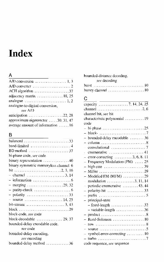
Index

AAID conversion 1, 3AID converter 2ACH algorithm 37adjacency matrix 18, 25analogue 1, 2analogue-to-digital conversion,

see AIDanticipation 22, 28approximate eigenvector 30, 31, 47average amount of information 16

Bbalanced 33band-limited 4BD method 37bi-phase code, see codebinary representation 40binary symmetric memoryless channel 6bit 2, 3,16- channel 3, 14- information 6- merging 29,32- parity-check 6- polarity 33- source 14, 25bit-stream 3, 43block 29block-code, see codeblock-decodable 29,37bounded-delay encodable code,

see codebounded-delay encoding,

see encodingbounded-delay method 36

bounded-distance decoding,see decoding

burst 10bursty channel 10

ccapacity 7, 14, 24, 25channel 2, 6channel bit, see bitcharacteristic polynomial 19code- bi-phase 25- block- 7- bounded-delay encodable 36- column 8- convolutional 7- enumerative 41- error-correcting 3, 6, 8, 11- Frequency Modulation (FM) 25- high-rate 39- Miller 29- Modified FM (MFM) 29- modulation 3, 11, 14- periodic enumerative 43, 44- polarity-bit 33- prefix 5- principal-state

- fixed-length 32- variable-length 36

- product 8- ~eed-Solomon 10- row 8- source 5- symbol-error-correcting 10- turbo 7code sequence, see sequence

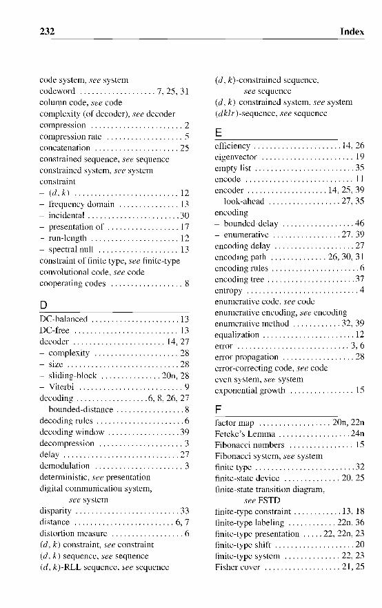
232

code system, see systemcodeword 7, 25, 31column code, see codecomplexity (of decoder), see decodercompression 2compression rate 5concatenation 25constrained sequence, see sequenceconstrained system, see systemconstraint- (d, k) 12- frequency domain 13- incidental 30- presentation of 17- run-length 12- spectral null 13constraint of finite type, see finite-typeconvolutional code, see codecooperating codes 8

DDC-balanced 13DC-free 13decoder 14,27- complexity 28- size 28- sliding-block 20n, 28- Viterbi 9decoding 6, 8, 26, 27- bounded-distance 8decoding rules 6decoding window 39decompression 3delay 27demodulation 3deterministic, see presentationdigital communication system,

see systemdisparity 33distance 6, 7distortion measure 6(d, k) constraint, see constraint(d, k) sequence, see sequence(d, k)-RLL sequence, see sequence

Index

(d, k)-constrained sequence,see sequence

(d, k)-constrained system, see system(dklr)-sequence, see sequence

Eefficiency 14, 26eigenvector 19empty list 35encode 11encoder 14,25,39- look-ahead 27, 35encoding- bounded-delay 46- enumerative 27, 39encoding delay 27encoding path 26, 30, 31encoding rules 6encoding tree 37entropy 4enumerative code, see codeenumerative encoding, see encodingenumerative method 32, 39equalization 12error 3,6error propagation 28error-correcting code, see codeeven system, see systemexponential growth 15

Ffactor map 20n, 22nFeteke's Lemma 24nFibonacci numbers 15Fibonacci system, see systemfinite type 32finite-state device 20, 25finite-state transition diagram,

see FSTDfinite-type constraint 13, 18finite-type labeling 22n, 36finite-type presentation 22, 22n, 23finite-type shift 20finite-type system 22, 23Fisher cover 21, 25

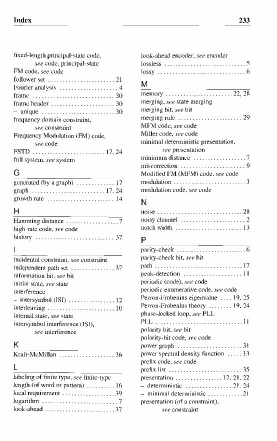
Index

fixed-length principal-state code,see code, principal-state

FM code, see codefollower set 21Fourier analysis 4frame 30frame header 30- unique 30frequency domain constraint,

see constraintFrequency Modulation (FM) code,

see codeFSTD 17, 24full system, see system

Ggenerated (by a graph) 17graph 17, 24growth rate 14

HHamming distance 7high-rate code, see codehistory 37

incidental constraint, see constraintindependent path set 37information bit, see bitinitial state, see stateinterference- intersymbol (lSI) 12interleaving 10internal state, see stateintersymbol interference (lSI),

see interference

KKraft-McMillan 36

Llabeling of finite type, see finite-typelength (of word or pattern) 16local requirement 39logarithm 7look-ahead 37

233

look-ahead encoder, see encoderlossless 5lossy 6

Mmemory 22, 28merging, see state mergingmerging bit, see bitmerging rule 29MFM code, see codeMiller code, see codeminimal deterministic presentation,

see presentationminimum distance 7miscorrection 9Modified FM (MFM) code, see codemodulation 3modulation code, see code

1\1noise 28noisy channel 2notch width 13

pparity-check 6parity-check bit, see bitpath 17peak-detection IIperiodic (code), see codeperiodic enumerative code, see codePerron-Frobenius eigenvalue 19, 25Perron-Frobenius theory 19, 24phase-locked loop, see PLLPLL 11polarity bit, see bitpolarity-bit code, see codepower graph 31power spectral density function 13prefix code, see codeprefix list 35presentation 17, 21, 22- deterministic 21, 24- minimal deterministic 21presentation (of a constraint),

see constraint

234

presentation of finite type,see finite-type

principal state, see stateprincipal-state method 26, 32, 36product code, see code

Qquantization 4quantization noise 4

Rrate 6, 14rate-distortion theory 6RDS, see running digital sumreceiver 2, 3redundancy 3,4,6, 14Reed-Solomon code, see coderegular language 22,24nreliability information 3reversed order 42row code, see coderun-length constraint, see constraintrunning digital sum (RDS) 13

ssampling 4sampling theorem 4saturation recording 11sender 2sequence- (d,k) 12- (d, k)-RLL 12- (d, k)-constrained 12- code 14- constrained 13- (dklr)- 29, 32Shannon cover 21shift, see under systemshift of finite type, see finite-typesignal 3size (of decoder), see decodersliding-block decoder, see decodersofic shift 25sofic system, see systemsource 4source bit, see bit

Index

source code, see codesource coding 4-6source data 2source symbol, see symbolsource-to-codeword assignment ..... 32spectral null constraint, see constraintspectral shaping 13state 17- initial 17, 18,36- internal 25- principal 26, 32- sub- 38- terminal 17, 40state merging 21, 35state-combination 37state-splitting 22, 37- ae-consistent 38- weighted 38storage system, see systemsub-state, see statesubset construction 22substitution method 27, 36subword-closed 24nsum-variance 13symbol- source 25,27,31,35symbol-error 10symbol-error-correcting code,

see codesymbolic dynamics 22n, 25synchronization 26, 29synchronous 25system 25- code 14, 31- constrained 14, 25- digital communication 2- (d,k)-constrained 17- even 20- Fibonacci 14, 16-18,20,43- full 21- sofic 20,22n,23,24,24n,25- storage 2- transmission 2system of finite type, see finite-type

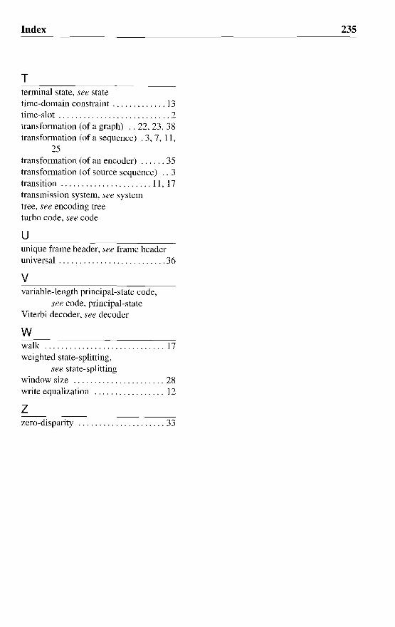
Index

Tterminal state, see statetime-domain constraint 13time-slot 2transformation (of a graph) .. 22.23,38transformation (of a sequence) . 3, 7, II,

25transformation (of an encoder) 35transformation (of source sequence) .. 3transition II, 17transmission system, see systemtree, see encoding treeturbo code, see code

uunique frame header, see frame headeruniversal 36

vvariable-length principal-state code,

see code, principal-stateViterbi decoder, see decoder

wwalk 17weighted state-splitting,

see state-splittingwindow size 28write equalization 12

zzero-disparity 33

235

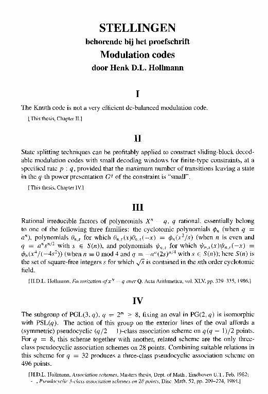
STELLINGENbehorende bij het proefschrift

Modulation codesdoor Henk D.L. Hollmann

IThe Knuth code is not a very efficient dc-balanced modulation code.

[This thesis, Chapter 11.]

IIState splitting techniques can be profitably applied to construct sliding-block decod­able modulation codes with small decoding windows for finite-type constraints, at aspecified rate p : q, provided that the maximum number of transitions leaving a statein the q-th power presentation Gq of the constraint is "small".

[This thesis, Chapter IV.]

IIIRational irreducible factors of polynomials xn - q, q rational, essentially belongto one of the following three families: the cyclotomic polynomials ¢n (when q =an), polynomials en,s for which en,s(x)8n,s(-x) = ¢n(x2 /s) (when 17 is even andq = a nsn/2 with S E Sen)), and polynomials 1f!n,s for which 1f!n,s(x)1f!n,s(-x) =¢n(x4/(-4s2 )) (when n == 0 mod 4 and q = -an (2s)n/4 with S E Sen)); here Sen) isthe set of square-free integers S for which v's is contained in the nth order cyclotomicfield.

[H.D.L. Hollmann, Factorization ofx N - q over Q, Acta Arithmetica, vol. XLV, pp. 329-335, 1986.]

IVThe subgroup of PGL(3, q), q = 2m ::: 8, fixing an oval in PG(2, q) is isomorphicwith PSL(q). The action of this group on the exterior lines of the oval affords a(symmetric) pseudocyclic (q/2 - I)-class association scheme on q(q - 1)/2 points.For q = 8, this scheme together with another, related scheme are the only three­class pseudocyclic association schemes on 28 points. Combining suitable relations inthis scheme for q = 32 produces a three-class pseudocyclic association scheme on496 points.

[H.D.L. Hollmann, Association schemes, Masters thesis, Dept. of Math., Eindhoven V.T., Feb. 1982;-, Pseudocyclic 3-class association schemes on 28 points, Disc. Math. 52, pp. 209-224, 1984.]

vWide-sense non-blocking self-routing switching networks between N senders andM receivers, constructed from switches that employ fixed-directory techniques, neces­sarily contain approximately N M switches; minimal networks can always be realizedby employing switches of four special types only.

[H.D.L. Hollmann J.H. v. Lint, Jr., Nonblocking self-routing switching networks, Disc. Appl. Math.,vol. 37/38. pp. 319-340, 1992.L. Halpenny and C. Smyth, Minimal nonblocking standard-path networks, Electr. Lett. 28-12,pp. 1107-1108, 1992.-, A classification ofminimal standard-path 2 x 2 switching networks, J. TheoL Camp. Sc., vol. 102,pp. 329-354. 1992.]

VI

~ ~~~ ].10 196

Here an * indicates an empty cell; the first 35 columns of B correspond to the 35 sub­sets of size three from {l, ... , 7}.

We say that an array B can be obtained from an array A of equal size by a rov.'-sln~tfle

if each row of B only contains entries from the corresponding row of A; a column­shuffie is defined similarly. With these definitions, each array B can be obtained froma given array A of equal size that contains each entry from B, by a sequence of atmost five row- or column-shuffles starting with a row-shuffle; this is no longer truewhen "five" is replaced by "four", as shown, e.g., by the arrays

A~[9: + i~6l B~[H H[RJ. Sluijter, H.D.L. Hollmann, C.M. Huizer, and H. Dijkstra, Coupling network for a data processor,including a series connection ofa cross-bar switch and an array ofsilos, U.S. patent 5280620, 1994.]

VII

We consider on-line source coding of a file of length N over an r-symbol alphabet{I, ... , r} (typically, r = 2m ), in which letter i occurs PiN times, by means of abinary uniquely decodable code C = {cl, ... , cr }. Write di to denote the length ofthe encoding Ci of the letter i. Let L = L;=l Pidi denote the average length of anencoded symboL let H = L;=l -Pi log Pi denote the entropy of the file, and leti5 = LUld,>logr pi(di -log r) be the maximum data expansion in bits per symbol. (Ifr = 2m

, then each letter in the file occupies m bits; if now all letters i with di > m arein the initial part of the file, then on-line encoding of the file will at first result in anexpansion of the file, where the maximal increase of the length is N i5 bits, before thefile starts to shrink.) With these definitions, i5 - L + H < I holds. If C is a Huffmancode, then (Huffman codes are optimal) L < H + I, so the above result implies thati5 < 2, improving the bound i5 :::: 4 in [1].

[[I] J-F. Cheng et. aI., Data expansion with Huffman codes, Proc. ISlT, Whistler, Canada, pp. 325, 1995.]

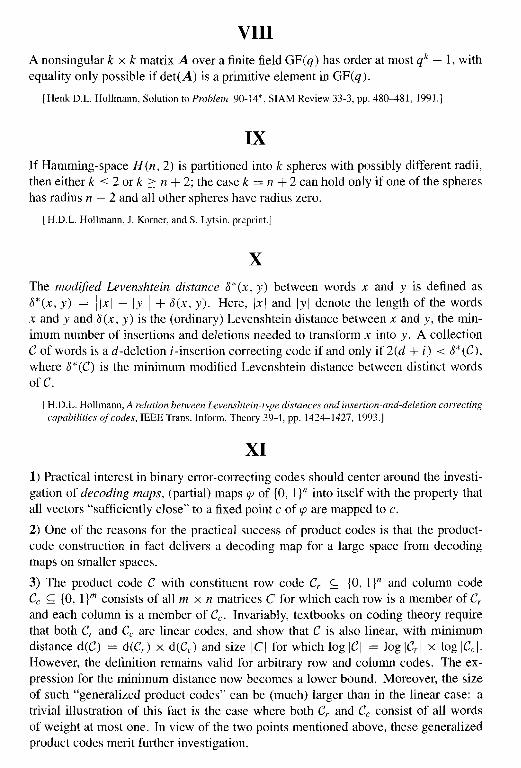
VIIIA nonsingular k x k matrix A over a finite field GF(q) has order at most qk - 1, withequality only possible if det(A) is a primitive element in GF(q).

[Henk D.L. Hollmann, Solution to Problem 90-14*, SIAM Review 33-3, pp. 480-481, 1991.]

IXIf Hamming-space H (n, 2) is partitioned into k spheres with possibly different radii,then either k :::: 2 or k ~ n + 2; the case k = n + 2 can hold only if one of the sphereshas radius n - 2 and all other spheres have radius zero.

[H.D.L. Hollmann, J. Korner, and S. Lytsin. prcprint.J

XThe modified Levenshtein distance 8*(x, y) between words x and y is defined as8*(x, y) = Ilxl - IYII + 8(x, y). Here, Ixl and Iyl denote the length of the wordsx and y and 8(x, y) is the (ordinary) Levenshtein distance between x and y, the min­imum number of insertions and deletions needed to transform x into y. A collectionC of words is ad-deletion i-insertion correcting code if and only if 2(d + i) < 8*(C),where 8*(C) is the minimum modified Levenshtein distance between distinct wordsofC.

rH.D.L. Hollmann, A relation between Levenshtein-type distances and insertion-and-deletion correctingcapabilities ofcodes, IEEE Trans. Inform. Theory 39-4, pp. 1424-1427, 1993.J

XI1) Practical interest in binary error-correcting codes should center around the investi­gation of decoding maps, (partial) maps cp of {a, 1}1l into itself with the property thatall vectors "sufficiently close" to a fixed point c of cp are mapped to c.

2) One of the reasons for the practical success of product codes is that the product­code construction in fact delivers a decoding map for a large space from decodingmaps on smaller spaces.

3) The product code C with constituent row code Cr <; {a, l}1l and column codeCc <; {a, l}m consists of all m x n matrices C for which each row is a member of Crand each column is a member of Cc . Invariably, textbooks on coding theory requirethat both Cr and Cc are linear codes, and show that C is also linear, with minimumdistance d(C) = d(Cr) x d(Cr> and size ICI for which log ICI = log ICrl x log ICc /'

However, the definition remains valid for arbitrary row and column codes. The ex­pression for the minimum distance now becomes a lower bound. Moreover, the sizeof such "generalized product codes" can be (much) larger than in the linear case: atrivial illustration of this fact is the case where both Cr and Cc consist of all wordsof weight at most one. In view of the two points mentioned above, these generalizedproduct codes merit further investigation.

XIILet l3 = (B i liE /) be a family of subsets of a finite set V. Write r v to denote thenumber of i E 1 for which v E Bi • If maxVEB

jr v ~ IBi I - 1 for all i E 1, then there

exists a subset U of V for which 1 ~ IU n Bi I ~ IBi I - 1 for all i E 1.

XIIIWe consider ordering in binary sequence spaces, as introduced in [1]. In the nota­tion of [1] and [2], we have that T2(O, 2, 1) = (1/3) log(2 + yJ) and T2(O, 2, 2) =(l /6) log A, where A is the largest real zero of x 3 - 12x2 - 4x - 1 and the logarithmis to the base of two.

[[I] R. Ahlswede. J-P. Ye, and Z. Zhang, Creating order in sequence spaces with simple machines. In­form. and compo 89, pp. 47-94, 1990.[21 H.D.L. Hollmann and P. Vamoose. Entropy reduction, ordering in sequence spaces, and semigroupsofnon-negative matrices, Preprint "Diskrete Structuren in der Mathematik" 95-092, Universitat Biele­feld, Germany, 1995.]

XIVComputation of the inverse of an element in GF(22m

) from a given vector representa­tion can be implemented in hardware with approximately 23m XOR- and AND-gates;in general such an implementation is to be preferred over one that involves log-tables.

[H.D.L. Hollmann. Data processing method and apparatus for calculating a multiplicatively invertedelement ofa finite field, U.S. patent 4 989 171, 1991.]

XVThe length N = 2/1 split radix FFT algorithm requires the lowest possible number ofmultiplications and possesses a regular "butterfly" structure. These and other proper­ties range this algorithm among the best FFT methods presently available.

[Po Duhamel and H.D.L. Hollmann, Split radix FFTalgorithm, Electr. Letters 20-1, pp. 14--16, 1984.]

XVIThe theory concerning the endgame of the game of "GO" as developed by Berlekampis of theoretical value only.

[E.W. Berlekamp and D. Wolfe, Mathematical go endgames: Nightmaresfor the professional go player,Ishi Press International, San Jose, CA, 1994.]

XVIIOok beginnende bridgers dienen te worden onderwezen in het gebruik van transferbiedingen na een 1SA opening van de partner.