ADVERTIMENT. Lʼaccés als continguts dʼaquesta tesi queda ... · la existencia de un límite en...
202
ADVERTIMENT. Lʼaccés als continguts dʼaquesta tesi queda condicionat a lʼacceptació de les condicions dʼús establertes per la següent llicència Creative Commons: http://cat.creativecommons.org/?page_id=184 ADVERTENCIA. El acceso a los contenidos de esta tesis queda condicionado a la aceptación de las condiciones de uso establecidas por la siguiente licencia Creative Commons: http://es.creativecommons.org/blog/licencias/ WARNING. The access to the contents of this doctoral thesis it is limited to the acceptance of the use conditions set by the following Creative Commons license: https://creativecommons.org/licenses/?lang=en
Transcript of ADVERTIMENT. Lʼaccés als continguts dʼaquesta tesi queda ... · la existencia de un límite en...

ADVERTIMENT. Lʼaccés als continguts dʼaquesta tesi queda condicionat a lʼacceptació de les condicions dʼúsestablertes per la següent llicència Creative Commons: http://cat.creativecommons.org/?page_id=184
ADVERTENCIA. El acceso a los contenidos de esta tesis queda condicionado a la aceptación de las condiciones de usoestablecidas por la siguiente licencia Creative Commons: http://es.creativecommons.org/blog/licencias/
WARNING. The access to the contents of this doctoral thesis it is limited to the acceptance of the use conditions setby the following Creative Commons license: https://creativecommons.org/licenses/?lang=en

NOVEL APPROACHES IN THE
IDENTIFICATION OF PATHOGENIC
VARIANTS IN THE CLINICAL
DIAGNOSIS
Casandra Riera Ribas
Supervisor: Dr. Xavier de la Cruz
Tutor: Dr. Enric Querol
PhD thesis – Programa Biotecnologia
Dpt. Enginyeria Química, Biològica i Ambiental (UAB)
Vall d'Hebron Insitut de Recerca (VHIR)
July 2016


As güelos
iii

iv

DECLARATION
I hereby declare I myself carried out the work described in
this thesis, except where indicated in the text. The work presented
here took place in the group of Translational Bioinformatics at the
Vall d'Hebron Institut de Recerca under the supervision of the Dr.
Xavier de la Cruz Montserrat. Also, I declare that this thesis has not
been and will not be submitted in whole or in part to another Uni-
versity for the award of any other degree.
Signed:________________________________________________
Date:_________________________________________________
Casandra Riera
Barcelona
v

vi

ACKNOWLEDGEMENTS
El meu agraïment etern és, en primer lloc, pel Xavier, que
ha aconseguit infondre en mi veritable amor per la ciència en el
sentit més ampli i un esperit científic amb què mirar el món més
enllà d'aquest laboratori. Ha estat, sens dubte, el millor mentor en
aquest període anomenat "doctorat" en el qual, si de cas, m’he
doctorat de moltes coses. Totes, en part, gràcies a ell. Gràcies per
inspirar-me. M'has fet una persona més crítica, més curiosa, més
honesta i més empàtica. No sé si optaré al Nobel, però sens dubte
sóc millor persona. I d'això, el món també en necessita.
I just devora estau valtros, família. Gracis perquè sempre
m’heu recolzat, sempre heu estat allí encara que no tenguéssiu
massa clar què és això que feia. Sense valtros avui no seria aquí.
Moltes gracis per tot, molt abans d’aquesta tesi.
Y a ti, Ibán, que me aguantas todos los días y tampoco
recibes financiación del Ministerio. Gracias por subir tantos días
conmigo en bici el ‘Col du Vall d’Hebron’, por tantas comidas ricas
y tanto ánimo. Por contarle a los demás, orgulloso, que yo estaba
haciendo mi doctorado.
vii

I continuant amb les famílies, a tots els que heu format
part de la família del Xavier, des de la del IBMB fins a la que és
ara, al VHIR. Al Jordi, per la paciència en les meves primeres
passes amb Perl. A la Montse, per ser tan bona companya i
persona. Al Iago i al Santi i el seu patinet. Després al Sergi, que ha
estat un grandíssim company durant la tesi i del que he après
moltíssim, encara que no em passés a Python. Als que ara
m’acompanyen: a la Natàlia, la millor tècnic del món, a l’Elena,
l’Òscar i el Josu, als qui desitjo molta sort en els seus doctorats.
Sens dubte estar en aquest grup és una gran fortuna.
Al grupo de Marian, en especial a Raquel, con quien he
compartido tantísimos cafés quejándonos de todo. ¡Mucha suerte!
Vull agrair especialment a tots els que formen part dels
Amics del VHIR, perquè per la seva generositat sóc aquí. De cada
visita i cada testimoni he tret força per avançar la tesi. Es pot dir
que sou co-autors! En compartir-ho amb vosaltres he après a mirar
la feina des d’una altra perspectiva.
Sense sortir del VHIR, a tots els companys i col·laboradors
que han posat el seu gra per fer-nos un lloc en aquesta família de la
Vall d’Hebron i establir ponts amb la nostra feina. En especial a
l'equip del Joan Montaner; a la Sara Gutiérrez, l’Orland Díez, la
Gemma i companyia; al grup del Joan Seoane, a l'equip de la
Chays, als nostres veïns d’Estadística i a molts més.
viii

Als meus companys de pis al llarg d’aquests anys, en
especial a l’Òscar, qui em va presentar al que seria el meu director
de tesi. Gonzalo, Kike, …i Sílvia també! Sandra y Claudia, gracias,
lindas. A Neus, por estar siempre.
Als bons professors que m’ha portat fins aquí, des de
l’escola, l’institut, la universitat.
Accèssit pel Joan Miquel, qui em va salvar
(metafòricament) la vida, un divendres a la nit, al ajudar-me en
l’àrdua tasca d’entendre’m amb els estils de LibreOffice. Sense ell
aquesta tesi no tindria una correcta paginació ni capçaleres.
A tots els que en una plana no puc condensar, gràcies.
“Gràcies” és el millor Abstract per aquesta tesi.
ix

x

Un nuovo modo di vivere, con una nuova luce, nuovi
abiti, nuovi suoni, un nuovo modo di parlare, nuovi
colori, nuovi sapori... tutto nuovo!
Scion, scion. Scion, scion...
Caro Diario, Nanni Moretti
xi

xii

ABSTRACT
The rapid growth experienced by next-generation sequen-
cing techniques has fuelled the development of bioinformatic ap-
plications for the functional annotation and interpretation of the
variants identified. In fact, the use of these tools is becoming in-
creasingly popular, having been extended to the field of clinical dia-
gnosis. However, the average success rate of these methods is
around 80%, still well below the levels required for their independ-
ent use in diagnosis. In this thesis we address this problem with the
goal of extending the accuracy of pathogenicity predictors and thus
improve their applicability. We have approached this challenge from
four different directions. First, we have identified the existence of
an upper limit in the success rate of these tools and determined that
the approach known as "protein-specific" is a good option to sur-
pass this threshold. Second, we have applied this approximation to
Fabry disease, developing a predictor that identifies causal variants
with a success rate of 90-95%, comfortably competing with com-
mon methods (e.g. SIFT, PolyPhen-2, etc.). Thirdly, we have exten-
ded this approach to a set of 82 proteins, benchmarking the quality
of the resulting protein-specific predictors against that of standard
tools. Finally, we have proposed a new way to compare prediction
methods, based on the cost. This approach implicitly considers both
xiii

the disease and the associated treatments available. As a result, it
constitutes a criterion for selecting predictors adapted to the clinical
context.
xiv

RESUMEN
El rápido crecimiento experimentado por las técnicas de
secuenciación de última generación ha impulsado a su vez el desar-
rollo de aplicaciones bioinformáticas destinadas a la anotación fun-
cional e interpretación de las variantes identificadas. De hecho, el
uso de estas herramientas es cada vez más popular, habiéndose ex-
tendido al ámbito del diagnóstico clínico. Sin embargo, la tasa de
éxito promedio de estos métodos se sitúa en torno al 80 %, bastante
por debajo todavía de los niveles requeridos para su uso independi-
ente en casos de diagnóstico. En la presente tesis se aborda este
problema con la finalidad de extender la precisión de estos métodos
y así mejorar su aplicabilidad. Para ello abordamos este desafío
desde cuatro perspectivas distintas. En primer lugar, identificamos
la existencia de un límite en la tasa de acierto de estas herramientas,
y determinamos que la aproximación denominada “protein-specific”
(específica de proteína) es realmente prometedora. En segundo
lugar, aplicamos dicha aproximación al caso de la enfermedad de
Fabry, desarrollando un predictor que identifica sus variantes caus-
ales con una tasa de acierto del 90-95 %, compitiendo holgada-
mente con la de los métodos habitualmente utilizados (ej. SIFT,
PolyPhen-2, etc.). En tercer lugar, extendemos esta aproximación a
un conjunto de 82 proteínas, contrastando la calidad de los predicto-
xv

res específicos con la de un amplio conjunto de herramientas es-
tándar. Finalmente, proponemos una nueva forma de comparar los
métodos de predicción basada en el coste. Este planteamiento con-
sidera de forma implícita tanto la enfermedad como los tratamientos
asociados disponibles. Como resultado se presenta un criterio de se-
lección de predictores más adaptado al contexto clínico.
xvi

CONTENTS
1 INTRODUCTION: PRINCIPLES UNDERLYING THE PRE-
DICTION OF PATHOLOGICAL VARIANTS.............................1
1.1 IDENTIFYING PATHOGENIC MUTATIONS: FEW PRINCIPLES,
MANY APPROACHES........................................................................5
1.2 CHARACTERIZING THE IMPACT OF PROTEIN SEQUENCE
MUTATIONS.....................................................................................7
1.2.1 Conservation-related properties................................................7
1.2.2 Protein structure and stability-related properties....................13
1.3 OBTAINING THE PREDICTION MODEL.....................................18
1.4 THE MUTATION DATASETS......................................................21
1.5 ESTIMATING THE PREDICTION PERFORMANCE OF A MODEL...26
1.6 CONCLUSION..........................................................................29
2 THE BOTTLENECK IN PREDICTION METHODS...........31
2.1 THE PREDICTION OF PATHOLOGICAL VARIANTS ALONG TIME.33
2.2 HAVE WE REACHED AN UPPER LIMIT IN OUR ABILITY TO
PREDICT PATHOLOGICAL VARIANTS?............................................41
2.2.1 Mutation annotations and dataset heterogeneities...................42
2.2.2 Loss- versus Gain-of-function mutations................................44
2.2.3 Hidden biological factors........................................................45
2.3 IMPROVING THE PREDICTION MODEL.....................................46
2.3.1 The need for new attributes to represent mutation impact......47
xvii

2.3.2 Protein specific: a new technical approach to pathogenicity
prediction........................................................................................49
2.4 CONCLUSION..........................................................................52
3 BUILDING A PREDICTOR FOR FABRY DISEASE............53
3.1 THE DIAGNOSIS OF FD: AN OPEN PROBLEM...........................55
3.2 MATERIALS AND METHODS...................................................57
3.2.1 Fabry variant dataset...............................................................58
3.2.2 Characterization of sequence variants in terms of discriminant
properties.........................................................................................61
3.2.3 Building a method for the discrimination between pathological
and neutral variants.........................................................................63
3.2.4 Performance estimation..........................................................64
3.3 RESULTS AND DISCUSSION.....................................................66
3.3.1 Gauging the impact of GLA variants regarding structure and
sequence properties.........................................................................66
3.3.2 Development of the prediction method...................................74
3.3.3 Comparison with other predictors...........................................78
3.3.4 Using prediction reliability to enhance success rate...............80
3.3.5 Independent validation of the FD-specific predictor...............81
3.4 CONCLUSION..........................................................................82
4 PROTEIN-SPECIFIC AND GENERAL PATHOGENICITY
PREDICTORS...............................................................................85
4.1 WHY PROTEIN-SPECIFIC PREDICTORS?...................................87
4.2 MATERIALS AND METHODS...................................................89
4.2.1 The variant datasets................................................................89
4.2.2 Characterization of variants in terms of discriminant properties
........................................................................................................91
4.2.3 Building the predictor method................................................92
4.2.4 Performance assessment.........................................................93
4.2.5 External prediction methods...................................................93
xviii

4.3 RESULTS AND DISCUSSION.....................................................94
4.3.1 The performance of GM predictors varies across proteins......95
4.3.2 Obtention and characterization of protein specific predictors
(PSP)...............................................................................................98
4.3.3 The complementarity between PSP and GM.........................103
4.4 CONCLUSION........................................................................111
5 HOW MUCH DOES THIS COST?........................................113
5.1 MEASURING CLASSIFIER PERFORMANCE: AN OUTLINE........116
5.2 A SIMPLIFIED VERSION OF HEALTHCARE COST TO EVALUATE
PATHOGENICITY PREDICTORS......................................................123
5.2.1 Absolute cost is not a monotonic function of standard perform-
ance measures................................................................................124
5.2.2 VarCost: an alternative to absolute cost................................126
5.2.3 Profiling standard predictors with VarCost: discarding the
concept of the absolutely best predictor.........................................128
5.2.4 VarCost vs. AUC/ROC.........................................................131
5.3 CONCLUSION........................................................................133
6 GENERAL CONCLUSIONS..................................................135
7 APPENDICES...........................................................................139
APPENDIX 1...............................................................................141
APPENDIX 2...............................................................................151
APPENDIX 3...............................................................................155
8 BIBLIOGRAPHY.....................................................................159
xix

xx

1 INTRODUCTION:
PRINCIPLES
UNDERLYING THE
PREDICTION OF
PATHOLOGICAL
VARIANTS

The results presented in this chapter have been recently
published in WIREs (Riera et al. 2014).

Introduction: Principles underlying the prediction of pathological variants
Understanding the molecular-level impact of sequence
changes and its relationship to disease has been an important chal-
lenge for many years now (Perutz 1992; Knight 2009). However,
since the publication of the first human genome draft (Lander et al.
2001; Venter et al. 2001) and, particularly, after the significant drop
experienced by next-generation sequencing (NGS) costs (Mardis
2010; Sboner et al. 2011) this challenge has taken a new form. NGS
has put within our reach invaluable knowledge: the list of sequence
variants an individual carries. The benefits of this information to the
medical field are illustrated by the increasingly relevant role played
by exome sequencing in both the understanding of the genetic basis
of disease and its diagnosis. This began to take the place of tradi-
tional association studies as the method of choice for probing the
landscape of human variation (Bamshad et al. 2011; Stitziel et al.
2011; Gonzaga-Jauregui et al. 2012; Ku et al. 2012; Quesada et al.
2012; Li et al. 2013a). These advantages, however, come with a
price, as the number of variants provided by NGS is so large, that
confidently identifying their functional or phenotypic significance is
a tough task, and careful relevance-filtering protocols must be ap-
plied (Stitziel et al. 2011). On a small scale (for single patients), if
the number of retrieved variants is low, they can be functionally
tested using in vivo or in vitro experiments, whenever they exist.
However, this experimental approach is unfeasible for the thousands
of variants observed in large clinical labs or population studies. In
this context, the application of in silico pathogenicity prediction
tools appears as the most viable alternative for the interpretation of
variants. And, in fact, numerous in silico methods (Bromberg et al.
3

Introduction: Principles underlying the prediction of pathological variants
2008; Capriotti and Altman 2011; Shihab et al. 2012; Sim et al.
2012; Sunyaev 2012; Al-Numair and Martin 2013) have already
been developed for the analysis, prioritization, and interpretation of
variants and their effects, alongside different guidelines on how to
utilize sequencing information for clinical purposes (Richards et al.
2015; Matthijs et al. 2016). However, these tools are still immature
because they often include incomplete representations of relevant
properties such as the free energy change of a protein upon muta-
tion, or the function loss, etc. As a consequence, users are faced
with the problem of deciding which method is the most reliable or
the most suitable tool for their particular system, or to quantify the
risk entailed by the use of specific programs, etc.
The two following chapters cover the work presented in
Riera et al. (Riera et al. 2014). Chapter 1 mainly corresponds to a
work of revision of the state of the art in this field while Chapter 2
offers some fundamental results of the advance in these in silico
prediction methods.
In this Introduction, I will expose the basics of these tools
and describe the main principles on which pathogenicity prediction
methods are based. However, before going any further, I would like
to address a relevant terminological issue related to how we refer to
sequence variants, particularly those involving an amino acid re-
placement in the protein sequence. A non-exhaustive survey of the
literature quickly shows that those changes of the protein sequence
known to cause disease receive different names: deleterious alleles
(Sunyaev et al. 2001), damaging mutations (Adzhubei et al. 2010),
deleterious substitutions (Ng and Henikoff 2001), deleterious poly-
morphisms (González-Pérez and López-Bigas 2011), pathological
4

Introduction: Principles underlying the prediction of pathological variants
mutations (Ferrer-Costa et al. 2004), pathogenic deviations (Al-
Numair and Martin 2013), and so on. A similar situation happens
with those sequence variants that do not have an effect on human
health, which are referred to as tolerant substitutions (Ng and
Henikoff 2001), neutral variants (Sunyaev 2012), SNPs (Al-Numair
and Martin 2013) (Single Nucleotide Polymorphism: single nucle-
otide substitution with a frequency equal to, or larger, than 1% in
the population (Knight 2009)), neutral mutations (Ferrer-Costa et al.
2004), and so on. When this thesis started, there was no clear prefer-
ence and the nomenclature chosen heavily depended on the field.
That was when we wrote our initial article on the intrinsic limits of
pathogenicity predictions (Riera et al. 2014), and there we em-
ployed the terms ‘pathological mutations’ and ‘neutral mutations’.
We use this terminology in both this chapter and in the following, to
preserve the coherence between its contents and that of the article.
However, since then the terminological issue has been clarified (Vi-
hinen 2014a), and the term 'variant' is the most preferred in biomed-
ical/clinical applications. We have used this more recent termino-
logy in the remainder of this thesis, starting in the chapter devoted
to our Fabry-specific predictor (Chapter 3).
1.1 Identifying pathogenic mutations: few
principles, many approaches
Simply posed, the problem of identifying pathogenic muta-
tions would read like this: "to be able to tell whether a mutation in
the amino acid sequence of a human protein is going to affect the
health of its carrier". In this work, we will focus only on sequence
5

Identifying pathogenic mutations: few principles, many approaches
changes originating mendelian diseases. The natural approach to
this problem would be to start from the main biophysical and bio-
chemical principles that describe protein sequence, structure, and
function. However, as the field of protein structure prediction
clearly illustrates (Rost and Sander 1993; Cole et al. 2008;
Mechelke and Habeck 2013; Mirabello and Pollastri 2013), our un-
derstanding of these principles is good, but not enough for our pur-
pose. Indeed, we are still unable to accurately (within experimental
error margins) predict the structure of a protein, its in vivo stability
(which involves an exact knowledge of the cell milieu, a challenge
in its own right), and how function precisely depends on protein
structure, stability and on dynamic properties. Not only this, we are
unable to explain how all these effects are modulated or amplified
as we progress upwards in the biological hierarchy to give the final
phenotype of the mutation. This is the hard side of the problem.
However, in the definition above there is also a hint of how we can
solve it in a practical way: we can use empirical models that relate
several measures of the molecular impact caused by a sequence
change with the presence/absence of a given phenotype (disease).
Simply put, these empirical models are computer programs (or
equations with adjustable parameters) that, given a sequence change
in a protein, determine its molecular impact, and indicate whether
this impact is going to alter, or not, the function of the protein. To
develop these models, we need three things: a series of sequence
properties related to the molecular impact of a variant, a proper
computational tool for building the model, and mutation datasets,
which will be used for training purposes. We describe them below.
6

Introduction: Principles underlying the prediction of pathological variants
1.2 Characterizing the impact of protein se
quence mutations
At present, the attributes most broadly used for pathogeni-
city prediction belong to two broad families (Sunyaev 2012): (1) se-
quence conservation-related, which reflect functional relevance; (2)
protein structure-related, which reflect stability and functional rel-
evance.
1.2.1 Conservationrelated properties
Evolution can be seen as one huge in vivo experiment for
evaluating the impact of amino acid changes. Changes occur by a
stochastic mutation process and those with negative effects on fit-
ness tend to be rejected by natural selection. We can access to part
of this information using comparative genomics, by aligning se-
quences from the same protein in different species (Figure 1.1).
Even at the most basic level, this principle is remarkably helpful in
predicting the effects of alleles and the relative importance of sites
(Page and Holmes 1998). This idea has been experimentally demon-
strated in the case of the protein structure stability. For example, an
agreement has been found (Steipe et al. 1994) between experimental
∆∆G upon mutation and a simple measure of sequence conserva-
tion: −RT ln(fmut
/fwt
), where fmut
and fwt
are the frequency of the
mutant and wild-type residues in the protein’s multiple sequence
alignment (MSA). This relationship has been checked by several
authors, in SH3 (Maxwell and Davidson 1998; Di Nardo et al.
2003), thioredoxin (Godoy-Ruiz et al. 2005), and more generally by
Sanchez et al. (Sanchez et al. 2006). The latter, using a set of 2351
7

Characterizing the impact of protein sequence mutations
mutations in 44 proteins, found a significant correlation of 0.5
between experimental and evolutionary ∆∆G, although the correla-
tion dropped to 0.17–0.21 when the residues involved also had a
functional role.
These observations indicate that the distribution of disease-
associated mutations relative to conservation measures differs from
that of neutral mutations. This fact, confirmed by different authors
(Miller and Kumar 2001; Ferrer-Costa et al. 2002; Miller et al.
2003; Steward et al. 2003) is on the basis of their predictive power
(Figure 1.2). One of the clearest examples is provided by SIFT (Ng
and Henikoff 2001; Sim et al. 2012) where the expected frequency
of the variant amino acid at the mutation locus gives a good predict-
ive power.
8
Figure 1.1 Conservation-based properties vary with the protein family.Prediction methods take advantage of the fact that the conservation patternreflects a balance between structure- and function-related constraints.However, the performance of these methods may be substantially affected bythe alignment’s quality and by the fact that different families have differentdivergence patterns. Here, we illustrate the latter for two different families:(A) the highly conserved histone 3 protein, and (B) the more divergent ser-pin family. In (C), we show how the different conservation patterns of theseproteins translate to different distributions of Shannon’s entropy, a propertyused in some prediction methods.

Introduction: Principles underlying the prediction of pathological variants
Ferrer-Costa et al. (Ferrer-Costa et al. 2004) also found that
their method’s performance was approximately 84%, and 78% cor-
responded to the use of measures of sequence variability within the
protein family. There are more cases where pathogenicity predictors
use the pattern of sequence conservation. For example, in PAN-
THER-PSEC (Thomas et al. 2003) the authors employ the log like-
lihood ratio of the wild-type and the variant amino acids, in Poly-
Phen-2 (Adzhubei et al. 2010) and SNAP (Bromberg and Rost
2007) the authors use the frequencies from the profile of amino
acids from the MSA of the protein family, etc.
A natural question then arises: how should we measure
conservation to achieve an optimal prediction performance? There
are several ways to measure conservation (Valdar 2002), although,
in the prediction context, it is unclear which is preferable. Using a
set of 9,334 pathological mutations from UniProt/SwissProt and
11,732 neutral mutations, Ferrer-Costa et al. (Ferrer-Costa et al.
9
Figure 1.2 The contribution of different attributes. Conservation-basedmeasures have stronger discrimination abilities than sequence-based fea-tures: (A) elements of the Blosum62 matrix (B) Shannon’s entropy in the dis-crimination between pathological (red) and neutral mutations (green).

Characterizing the impact of protein sequence mutations
2004) found that performance varied with the chosen property:
Shannon’s entropy, which gives a simple idea of compositional di-
versity (Figures 1.1-1.2), gave approximately 67% accuracy; a more
elaborate measure, taken from Martin et al. (Martin et al. 2002),
gave about 68% accuracy; and pssm (position-specific scoring
matrices) and ∆pssm gave approximately 78% and 73% accuracies,
respectively. PolyPhen authors utilize PSIC (Sunyaev et al. 1999),
an index that in the development of PolyPhen-2 was chosen among
the best 11 predictors. SIFT uses a sophisticated version of pssm
giving 75–85% accuracies in UniProt/SwissProt datasets. In sum-
mary, although different measures of amino acid conservation pro-
duce comparable performance accuracies (70–85%), the different
variants of pssm generally give better results. However, this de-
pends on how they are implemented, as Reva et al. (Reva et al.
2011) successfully combine family and subfamily entropy in Muta-
tionAssessor (accuracy: 80%); and Shihab et al. ∼ (Shihab et al.
2012) list an 86% accuracy for their method, FATHMM, combining
variant frequencies and a Hidden Markov model.
We have just seen that conservation, measured at the amino
acid level, has an important contribution to the performance of pre-
diction methods. However, conservation can also be measured at the
DNA level, which permits the introduction of more refined evolu-
tionary models. Early work by Santibáñez-Koref et al. (Santibáñez-
Koref et al. 2003) deserves mention for their inclusion of DNA-
based phylogenetic trees, although their approach, technically com-
plex, was only tested in the case of TP53 mutations. More recently,
Capriotti et al. (Capriotti et al. 2008) utilized selective pressure (ω =
dN/dS; where dN is the non-synonymous substitution rate per non-
10

Introduction: Principles underlying the prediction of pathological variants
synonymous site, and dS the synonymous substitution rate per syn-
onymous site) obtaining a prediction accuracy of 82% in a set of
UniProt/SwissProt mutations. Chun and Fay (Chun and Fay
2009) used a Likelihood ratio test to check whether selective pres-
sures act on a specific codon versus the possibility that the codon is
evolving under a neutral model. The results obtained with a set of
5,493 and 39,028 pathological and neutral mutations gave 91% ac-
curacy (estimated from the data in the article). Mutation imbalance
between both mutation types (#pathol/#neutral = 0.14) partly ex-
plains this large accuracy value, the success rate for pathological
mutations is approximately 72%, comparable to that of the first
SIFT and PolyPhen versions (Chun and Fay 2009).
In summary, the results mentioned here suggest that, if
dataset size does not introduce a restriction on the number of attrib-
utes, it may be worthwhile to include more than one conservation
measure. At this stage, it must be noted that all of them have a fun-
damental limitation: they are all implicitly based on the assumption
of independence between MSA positions. However, this assumption
is not valid because protein residues are packed and folded into a
three-dimensional structure and carry out its function as a complete
sequence. There is ample evidence in biochemistry, biophysics, and
modern genetics that interactions between sites do exist and are im-
portant (Breen et al. 2012; Ashenberg et al. 2013; Corbett-Detig et
al. 2013; McCandlish et al. 2013). From the point of view of predic-
tion methods, this is important since residue-residue interactions
can compensate the pathogenic effect of a given amino acid replace-
ment (Kondrashov et al. 2002; Ferrer-Costa et al. 2007), and an ap-
parently pathogenic mutation may indeed be neutral. This may hap-
11

Characterizing the impact of protein sequence mutations
pen either through allosteric phenomena coupling very distant
residues (Sinha and Nussinov 2001; Cui and Karplus 2008) or
through interactions with close neighbours (Bagci et al. 2002).
Without specific biological or biochemical knowledge about the
protein in question, the relevant compensation could happen at any
position or combination of positions in the entire genome. Nonethe-
less, it is clear that prediction protocols must introduce neighbour
effects to really increase their present performance (Sunyaev 2012).
To close this section, I would like to focus on a key tech-
nical aspect, related to the way we measure conservation properties.
These properties are derived from the MSA, and for this reason the
MSA has an substantial impact on the success rates of predictors.
Obtaining an MSA is a classical and challenging problem in bioin-
formatics (Durbin et al. 1998) that first involves sequence retrieval
(usually done with programs from the Blast suite (Schäffer et al.
2001)) and then alignment of these sequences, using any of the
available methods (Sinha and Nussinov 2001). When few gene fam-
ilies are involved MSA can be built manually with good results
(Durbin et al. 1998); however, this is unfeasible when working with
large numbers of genes, and automatic methods are preferred. This
has an important limitation: the problem of building MSA is NP-
hard (Elias 2006), which in practical terms means that MSA has to
be built using heuristic methods (reviewed elsewhere (Do 2008))
that cannot guarantee that the optimal alignment is reached. The im-
pact of these problems has been analysed in the field of mutation
prediction by Hicks et al. (Hicks et al. 2011). These authors have
used a highly controlled system, constituted by BRCA1, MSH2,
MLH1, and TP53 genes, for which they retrieved a total of 267
12

Introduction: Principles underlying the prediction of pathological variants
mutations (52 neutral and 215 deleterious). They found that the
methods’ performances clearly depend on the MSA protocol (num-
ber of sequences and alignment nature), although SIFT and Poly-
Phen showed the lowest dependence on the MSA. Acting on these
results, SIFT developers modified their MSA protocol and obtained
an improved performance (Sim et al. 2012), thus confirming the rel-
evance of MSA quality. Within this context, we want to mention
that database composition biases can also affect conservation meas-
ures (Henikoff and Henikoff 1994), as for different reasons related
species may be overrepresented. This effect may be reduced using
different weighting schemes, although it does not seem too relevant
for the discrimination between pathological and neutral mutations
(Ferrer-Costa et al. 2002).
1.2.2 Protein structure and stabilityrelated properties
The structure of haemoglobin opened the way for the inter-
pretation of the effect of pathological mutations in terms of struc-
ture properties (Perutz 1992): ‘The haemoglobin molecule is insens-
itive to replacements of most amino acid residues on its surface but
extremely sensitive to even quite small alterations of internal non-
polar contacts ...’ (Perutz and Lehmann 1968) and ‘... it was also en-
couraging that many clinical symptoms could be interpreted at the
atomic level’ (Perutz 1992). This idea has been subsequently con-
firmed and refined by a vast number of structural studies. In particu-
lar, by site-directed mutagenesis studies that have contributed to cla-
rifying the relationship between structure-stability and function
(Creighton and Goldenberg 1992; Fersht 1998; Baase et al. 2010),
13

Characterizing the impact of protein sequence mutations
showing that many damaging mutations act by destabilizing protein
structure or interfering with its formation. These studies also have
provided a simple set of empirical rules relating mutation impact
and protein structure disruption. They can be grouped into two fam-
ilies: amino acid-level and structure-level properties. Amino acid-
level properties reflect the fact that the nature of the mutation may
already be an important destabilizing factor. For example, replacing
a small by a large residue is likely to disrupt protein structure,
something that happens in superoxide dismutase for the mutation
responsible for familial amyotrophic lateral sclerosis A4V, a muta-
tion that affects local packing (Cardoso et al. 2002; DiDonato et al.
2003) and as destabilizes the functional dimer (Figure 1.3). This ex-
ample also illustrates that the impact of a change depends on its
structural location: in this case, A4V is damaging because it hap-
pens at a nearly buried location close to the dimer interface.
14
Figure 1.3 Pathological mutations affect different aspects of protein func-tion. (A) Superoxide dismutase mutants A4V and H43R affect monomer anddimer stability, leading to aggregation and function loss. (B) Angiogeninmutant K40I directly affects the functional site as annotated in theUniProt/SwissProt database.

Introduction: Principles underlying the prediction of pathological variants
In general, it has been shown (Wang and Moult 2001; Fer-
rer-Costa et al. 2002; Yue et al. 2005) that neutral and pathological
mutations usually have different distributions over the range of
structure/stability-related descriptors. This supports both the idea
that many mutations are pathological because of their impact on
protein stability, and that simple structure properties can be used for
their identification. This hypothesis has been confirmed by the res-
ults of different in silico predictors (Chasman and Adams 2001;
Saunders and Baker 2002; Ferrer-Costa et al. 2004; Bao and Cui
2005; Karchin et al. 2005a; Karchin et al. 2005b; Yue et al. 2006;
Bromberg and Rost 2007; Barenboim et al. 2008; Adzhubei et al.
2010; Venselaar et al. 2010; Capriotti and Altman 2011; Stitziel et
al. 2011; Juritz et al. 2012; Wang et al. 2012; Al-Numair and Martin
2013). However, the contribution of structure attributes to the suc-
cess of prediction methods is lower than that of conservation meas-
ures (Sunyaev 2012). Ferrer-Costa et al. (Ferrer-Costa et al.
2004) found that, by itself, residue accessibility gave approximately
62% accuracy, lower than the 67% and 78% accuracies obtained
with Shannon’s entropy and pssm, respectively. This is not so sur-
prising, as in some cases, the relationship between simple structure
properties and the damaging effect of pathological mutations (e.g.,
mutations affecting the protein folding process or the catalytic site)
is at best unclear. Even when pathological mutations affect protein
stability, the most frequent case (Yue et al. 2005), it is not strange
that structure-based properties have a limited performance, as pre-
dicting protein stability changes upon mutation is a hard problem
(Khan and Vihinen 2010). This is because stability results from the
subtle balance of several complex terms, such as the hydrophobic
15

Characterizing the impact of protein sequence mutations
effect or the conformational entropy (Dill 1990), tough to model us-
ing only coarse-grained attributes. The origin of the problem also
suggests its solution, which would be a more detailed description of
the attributes representing stability changes, for example, using dis-
tance-based potentials, and so on. Such an approach has been tried
by Al-Numair and Martin (Al-Numair and Martin 2013) with really
promising results: their Random Forest-based predictor reaches an
approximately 85–90% accuracy.
Beyond technical issues, the use of structure attributes in
prediction methods is currently limited by the large gap existing
between sequence and structure (less than 1% of UniProt/SwissProt
sequences are mapped to an experimental structure), which means
that many mutations happen at protein locations where no structural
information is available. This gap can be partly closed using low-
resolution representations of protein structure, such as those
provided by secondary structure and accessibility predictions (Saun-
ders and Baker 2002; Krishnan and Westhead 2003; Ferrer-Costa et
al. 2004; Karchin et al. 2005b; Bromberg and Rost 2007); however,
the errors in these predictions may reduce the value of their contri-
bution to mutation prediction (Krishnan and Westhead 2003;
Bromberg and Rost 2007).
In summary, the use of structure-based properties improves
the performance of prediction methods, given the intimate relation-
ship between protein structure and function. And when combined
with conservation properties (Figure 1.4), they give an increased ac-
curacy. However, as shown by the fact that average prediction ac-
curacy is somewhere around 80%, it is clear that even when taken
together, these attributes may fail to identify mutations hitting func-
16

Introduction: Principles underlying the prediction of pathological variants
tionally relevant residues. Part of the accuracy gap can be closed us-
ing more refined representations of conservation and structure prop-
erties; alternatively, database annotations may provide a useful ap-
proach. These annotations can be divided into two broad classes:
residue level and network level. Residue-level annotations, which
are retrieved from general databases such as UniProt/SwissProt, dir-
ectly identify those residues that belong to active sites, bind sub-
strate (Figure 1.3B), are subject to post-translational modifications,
etc. If it is not too general (e.g., when residues are annotated as per-
taining to a domain that spans over the complete protein length),
this information can be included in any empirical model as a binary
variable (Witten and Ule 2011), although its true contribution is un-
clear in the case of general methods trained on large protein sets
(Yue et al. 2005; Ng and Henikoff 2006). However, in the case of
gene-specific predictors, it has been shown that these annotations
may enhance their success rate (Jordan et al. 2011).
17
Figure 1.4 The relationship between conservation-based andstructure attributes. For Uridine 5'-monophosphate synthase, weshow how the location of the substrate binding site (substrate inblue) is related to residue conservation, which is represented usinga green (high conservation) to white (low) color scale.

Characterizing the impact of protein sequence mutations
Annotations related to the interaction network of the pro-
tein serve to bring the prediction problem within a broader and
more powerful biological context. As noted by Khurana et al.
(Khurana et al. 2013) ‘... a moderately deleterious missense SNV in
a highly significant gene can be equally or more damaging than a
strongly deleterious missense SNV in a less significant gene’. Con-
sequently, use of gene network information should enhance the pre-
diction of pathological mutations. Huang et al. (Huang et al.
2010) have followed this approach, combining sequence, structure,
and network-based properties in a single method. When tested in a
large UniProt/SwissProt set of mutations, the authors obtained an
approximate accuracy of 83% (71% accuracy was obtained for
SIFT). In their analysis of the individual contribution of each attrib-
ute, Huang et al. found that the major contributor to the method’s
performance was the KEGG (Kotera et al. 2012) enrichment score,
a network-based property. On the same line, but using GO (Ash-
burner et al. 2000) as an information source on the protein’s biolo-
gical context, Calabrese et al. (Calabrese et al. 2009) combined dif-
ferent attributes in their prediction model. These authors also ob-
served that inclusion of network information improved the perform-
ance of their method by approximately 10% (Table 1 in Calabrese et
al. 2009).
1.3 Obtaining the prediction model
Once we have identified the main principles determining
the impact of a sequence variant, we need to combine them quantit-
atively, in a predictive model that will generate the corresponding
impact estimations. The main steps followed in the design of such
18

Introduction: Principles underlying the prediction of pathological variants
model are represented in Figure 1.5; in this and the next sections,
we will cover all of them.
19
Figure 1.5 The four steps in the development of a method forthe prediction for pathological mutations. The first step is theobtention of the mutation dataset, which must include enoughpathological and neutral mutations to reliably derive all theparameters in the model. Next, we must decide what parametersprovide the best representation for the relationship betweenmutation damage and disease phenotype. Two families of para-meters are generally used: sequence-conservation properties,and structure-related properties such as residue accessibility,secondary structure propensities, and so on. In the third step, themodel is produced using one of the many possible availabletechniques. Finally, once the model is obtained, its performanceis estimated, so that users may judge to which extent it is ad-equate for their goals.

Obtaining the prediction model
Since there are no exact formal models to combine all
these heterogeneous information sources, we must resort to empiric-
al models. Fortunately, the machine learning field provides a broad
range of approaches and software suites that facilitate this task. In
fact, the problem of discriminating between two mutation types us-
ing a set of attributes is analogous to many pattern recognition prob-
lems, and for this reason can be addressed using the powerful ma-
chinery of the field (for a detailed introduction, which includes a
certain amount of mathematics, readers are referred to the books by
Bishop (Bishop 1995; Bishop 2006), Hastie et al. (Hastie et al.
2009), and Duda et al. (Duda et al. 2001); those preferring a more
applied view will enjoy the book by Witten et al. (Witten and Ule
2011), which also gives an introduction to the WEKA package). In
fact, bioinformatics research abounds (Baldi and Brunak 2001) with
examples where comparable problems have been addressed using
neural networks, support vector machines, etc. From these studies,
one can draw valuable lessons on how to normalize variables, bal-
ance the training sample, encode qualitative properties, and so on.
This is particularly true with the field of secondary structure predic-
tion where substantial improvements (Qian and Sejnowski 1988;
Rost and Sander 1993) were obtained through the use of neural net-
works, and where consensus methods were derived to improve pre-
diction performance (Cole et al. 2008).
At a practical level, different tools can be used for the pre-
diction of pathological mutations (neural networks (Ferrer-Costa et
al. 2004), SVMs (Capriotti et al. 2008; Calabrese et al. 2009), Ran-
dom Forests (Al-Numair and Martin 2013), Naïve Bayes classifiers
(Adzhubei et al. 2010), etc.). In fact, we cannot say which one is
20

Introduction: Principles underlying the prediction of pathological variants
preferable, as they are usually tested in slightly different mutation
datasets and under similar, but not always equal properties/attrib-
utes. Moreover, at the point in which we are in the prediction prob-
lem, when the type and number of attributes is not yet completely
defined, issues like an easy interpretation of the prediction process
may take priority when deciding how to build the model. In this
sense, there is an interesting study in which Krishnan and Westhead
(Krishnan and Westhead 2003) compared the performance of de-
cision trees and SVMs on the same dataset, finding that SVMs had
a slightly better success rate that decision trees, but the latter gave
prediction rules easier to interpret.
1.4 The mutation datasets
Once obtained, the predictor is an empirical model, imple-
mented in a computer program, and defined by a series of paramet-
ers. These parameters are obtained in a cyclic learning process
where the program is presented with a series of known data, gener-
ates predictions, these predictions are compared with the observa-
tions, corrections ensue, and the cycle starts again. In our case, the
training data are the mutation datasets and are made of both patho-
genic and neutral mutations. We describe them below.
Mutation datasets are intimately related with the prediction
goal. If we are interested in a single gene or group of genes, our
method should be made specific by restricting our data to mutations
affecting these genes only (Ferrer-Costa et al. 2004; Jordan et al.
2011; Crockett et al. 2012). If we want to score large numbers of
variants from many genes, for example, when processing data from
an exome project, methods trained on big, heterogeneous datasets
21

The mutation datasets
are preferable, as methods trained on specific genes will give poorer
predictions when applied to other genes (Care et al. 2007). Datasets
not only determine the value of the parameters in the model,
through the fitting process, they also implicitly define an upper
threshold for the number of parameters (Bishop 2006; Witten and
Ule 2011), if we are to avoid overfitting. This is an important issue
when deriving empirical models, in which the number of parameters
and their relationships are a priori unclear, and one may decide to
use feature selection procedures before building the model (Cline
and Karchin 2011). In our case, datasets are constituted by two
mutation types: pathological and neutral. In general, pathological
mutations are obtained from central variation databases like Uni-
Prot/SwissProt (Yip et al. 2008), Online Mendelian Inheritance in
Man (OMIM) (Amberger et al. 2009), Human Gene Mutation Data-
base (HGMD) (Stenson et al. 2014), VariBench (Sasidharan Nair
and Vihinen 2013), or from Locus-specific variation databases that
list variants in specific genes/diseases and are typically manually
annotated (like those grouped in Leiden Open Variation Database
(LOVD) (Fokkema et al. 2011) or in the Human Genome Variation
Society (HGVS) website). These databases are usually the most
trusted variation information sources as they are curated and main-
tained by experts in the genes and diseases. Other source of patho-
genic mutations is large mutagenesis experiments, such as the ones
in HIV-1 protease (Loeb et al. 1989), T4 lysozyme (Rennell et al.
1991) and Lac repressor (Suckow et al. 1996).
UniProt/SwissProt (Yip et al. 2008) and HGMD (Stenson
et al. 2003) provide the largest number of pathological mutations, a
number well over 20,000, although the actual figure is hard to know
22

Introduction: Principles underlying the prediction of pathological variants
as these databases are periodically updated, and in the case of
HGMD, part of the data is available after subscription. Until now,
UniProt/SwissProt has been the choice source in many cases, for
example, in the PolyPhen family (Sunyaev et al. 2001; Adzhubei et
al. 2010), in PMut (Ferrer-Costa et al. 2004; Ferrer-Costa et al.
2005a), in PhD-SNP (Capriotti et al. 2006), and so on. It should be
noted that mutation annotation protocols vary between databases
and for this reason may result in discrepancies between them.
For neutral mutations, the situation is slightly more com-
plex: UniProt/SwissProt provides a list of neutral variants, which is
at present over 38,000, but dbSNP (Sherry et al. 2001) (which con-
tains data from The 1000 Genomes Project, www.1000-gen-
omes.org), is also an important source, as after implementing some
filters (e.g., population frequency), we can retrieve over 20,000
neutral variants (Thusberg et al. 2011). Other large projects such as
Exome Aggregation Consortium (ExAC, exac.broadinstitute.org)
has data from over 60,000 unrelated individuals and Allele Fre-
quency Community (AFC, www.allelefrequencycommunity.org)
currently contains data for about 100,000 exomes/genomes. The
University of California, Santa Cruz (UCSC) Genome Browser
(Kent et al. 2002), the National Center for Biotechnology Informa-
tion (NCBI) Map Viewer (Wheeler et al. 2004), the Ensembl Gen-
ome Browser (Stalker et al. 2004), and others provide information
about genes, their products, and sequence variants.
However, when using these data, some issues must be con-
sidered: annotated polymorphisms may be deleterious under some
conditions (Ng and Henikoff 2006), and even SNP frequency is not
a complete guarantee that it will not be deleterious. An alternative to
23

The mutation datasets
these sets of neutral mutations is the use of ‘divergence data’ (Sun-
yaev et al. 2001), where sequence differences between the human
proteins and their closest homologs are labelled as neutral. Of
course, some restrictions are applied to ensure that the variants re-
trieved have little impact on protein function, for example, only
close mammalian sequences are considered (Adzhubei et al. 2010),
or homologs must be highly similar to the human protein (Ferrer-
Costa et al. 2004) or must have the same function as the human pro-
tein (Bromberg and Rost 2007). In spite of these controls, some of
the retrieved variants may actually be pathological because in the
non-human species, their damaging effect is rescued by compensat-
ory mutations (Ferrer-Costa et al. 2007; Baresic et al. 2010). In gen-
eral, database mutations sets provide enough data to develop gener-
al predictors of different complexity with reasonably good success
rates (70–90%) (Bao and Cui 2005; Ferrer-Costa et al. 2005a;
Capriotti et al. 2006; Yue et al. 2006; Bromberg et al. 2008; Capri-
otti et al. 2008; Li et al. 2009; Adzhubei et al. 2010; Schwarz et al.
2010; Li et al. 2011; Thusberg et al. 2011; Lehmann and Chen 2012;
Li et al. 2012; Lopes et al. 2012; Shihab et al. 2012; Sunyaev 2012;
Wang et al. 2012; Al-Numair and Martin 2013; Thompson et al.
2013).
An interesting alternative to database mutation lists is the
use of large mutagenesis experiments. These experiments have been
carried on microbial systems and together provide nearly 6400
mutations, of which approximately 2600 affect the phenotype. The
advantage of these experimentally derived datasets is that they are
unbiased relative to mutation location (Ng and Henikoff 2001), as
all positions have been mutated. On the other side, they may have a
24

Introduction: Principles underlying the prediction of pathological variants
stronger gene bias than database mutation lists, as they represent
three proteins only (Lac repressor, HIV-1 protease and T4 lyso-
zyme). Also, because the number of mutations is around an order of
magnitude less than that of database-derived lists, the maximum
complexity of the trained models is somewhat restricted. Having
said that, it is undeniable that they capture an important part of the
essence of the prediction problem, as after their original use in the
obtention and benchmarking of SIFT (Ng and Henikoff 2001), they
have been used in the development of other methods of different
complexities (Saunders and Baker 2002; Krishnan and Westhead
2003; Cai et al. 2004; Stone and Sidow 2005; Karchin et al. 2005b;
Marini et al. 2010).
As we have seen, there are several options to train our pre-
dictions, and it is unclear which one is best. In front of this problem,
Care et al. (Care et al. 2007), after comparing different datasets, ad-
vocate for UniProt/SwissProt-based pathological and polymorphism
collections; however, they leave the door open to the use of other
collections, depending on the set of attributes chosen and the
user/developer’s goal. Adzhubei et al. (Adzhubei et al. 2010), on the
basis of evolutionary considerations, indicate that for mendelian
disease diagnosis UniProt/SwissProt polymorphisms constitute a
good neutral model, whereas the use of homolog-based variants as
neutral mutations may be preferable for the case of complex pheno-
types. Finally, Al-Numair and Martin (Al-Numair and Martin
2013) provide an interesting framework to assess dataset selection,
and its impact on prediction performance, when discussing database
composition from the point of view of mutation penetrance (the fact
25

The mutation datasets
that the effect of a mutation also depends on variables (Cooper et al.
2013) such as environment, existence of modifier genes, etc.).
1.5 Estimating the prediction performance
of a model
Our predictor is obtained applying a data fitting procedure,
after which the method’s performance is assessed (Witten and Ule
2011). As mentioned in section 1.1, if several models are available,
it is important to choose the one that best captures the differences
between the two populations. However, this natural strategy also en-
tails a substantial risk, the risk of overfitting. This means that the al-
gorithm adapts so closely to our training dataset that it ends up
learning all the noise or random features in the training dataset, con-
fusing them with true properties of neutral and pathogenic muta-
tions (Witten and Ule 2011). These issues have to be taken into ac-
count before making any decision based on success rates.
To estimate the prediction performance, manual analysis of
the results (Figure 1.6) may serve as a guide about the potential of a
predictor. However, more quantitative and objective protocols must
be applied. N-fold cross-validation is one of the most common
(Witten and Ule 2011), and certainly the most widely used in the
prediction of pathological mutations. The standard cross-validation
protocol involves the following steps (Krishnan and Westhead 2003;
Witten and Ule 2011): (1) divide the original mutation set in N
parts; (2) use (N-1) parts to train the predictor, and the remaining
part to estimate its performance; (3) repeat step (2) until each of the
N parts has been left outside the training set once; and (4) average
26

Introduction: Principles underlying the prediction of pathological variants
the N estimates to give the cross-validation estimate of the method’s
performance.
This general procedure admits an interesting variant in the
case of mutation predictors, called heterogeneous cross-validation
(Krishnan and Westhead 2003), in which an additional restriction is
added in step (2): the same protein must not simultaneously contrib-
ute mutations to the training and to the test sets. When mutations in
the original dataset are distributed over a large number of proteins,
this approach is valuable as it may provide a more reliable estimate
of a method’s performance (note that this may depend on factors
such as the number of duplicates per gene family and their distribu-
tion between training and test sets). However, for methods trained
27
Figure 1.6 Correctly and incorrectly predicted mutations. Visual ana-lysis of the mutations may serve to confirm the prediction ability of amethod: P112L mutation in angiogenin was correctly predicted aspathological, probably because of its proximity to the catalytic triad.Visual analysis may also help us to identify weak points in predictions:why S28N mutation was incorrectly predicted as neutral?

Estimating the prediction performance of a model
with a small number of protein families in mind, heterogeneous
cross-validation may result in more pessimistic estimates. In this
case, the homogeneous cross-validation scheme (in which steps (1)–
(4) are applied to each protein separately) is preferable. Until now,
we have spoken about performance in an abstract way, or giving
only accuracy figures. However, accuracy (1.1) may be misleading
when there is an imbalance in the mutation dataset (Vihinen 2012a).
In fact, the best option to describe the performance of a predictor is
to provide several measures (Baldi et al. 2000; Vihinen 2012a). Ac-
curacy is defined as:
Accuracy=TP+TN
TP+ FN+TN +FP(1.1)
where TP and TN are the number of true positives and negatives, re-
spectively; and FP and FN are the number of false positives and
negatives, respectively. Apart from accuracy, a parameter cited in
many works is MCC (1.2), the Matthews correlation coefficient is
described as:
MCC=TP·TN−FP·FN
√(TP+FN ) ·(TN +FP) ·(TP+FP)·(TN+FN ) (1.2)
The values of MCC vary between 1 and −1, which corres-
pond to complete agreement and disagreement in the predictions,
respectively; for random predictions, MCC is equal to 0 (Baldi et al.
2000). We would like to mention that in recent years ROC curves
have also been utilized to characterize and compare the performance
of predictors (Calabrese et al. 2009; Adzhubei et al. 2010;
González-Pérez and López-Bigas 2011; Lopes et al. 2012; Sim et al.
2012).
28

Introduction: Principles underlying the prediction of pathological variants
1.6 Conclusion
Since their appearance in the early 2000s, the interest in the
methods for the prediction of pathological mutations of the protein
sequence has raised continuously. These methods are based on the
intimate relationship between protein structure and function. In one
way or another, essentially all of them represent the relationship
between mutation impact and disease utilizing one, or both, of the
following families of properties: conservation-related and structure-
related. The former are based on the use of MSAs, whereas the lat-
ter are based on structure information, either observed or inferred,
and on the properties of the amino acid change (e.g., hydrophobicity
and volume change, mutation matrices like Blosum or PAM, etc.).
Using different computational approaches to combine this informa-
tion, these methods have reached a prediction accuracy in the 70–
90% range, with an increasingly good balance between the predic-
tion success of pathological and neutral mutations.
29


2 THE BOTTLENECK IN
PREDICTION METHODS
(CAN WE SURPASS IT?)

The results presented in this chapter have been recently
published in WIREs (Riera et al. 2014).

The bottleneck in prediction methods
As we have seen in the Introduction, more than 10 years
have passed since the first method for the prediction of pathological
mutations were published (Ng and Henikoff 2001; Sunyaev et al.
2001). During this time their use has increased rapidly; for example,
PolyPhen-2 and SIFT gather 1645 and 816 citations (Katsonis et al.
2014), they are both included as a default in the VariantStudio soft-
ware from Illumina (used for the analysis of sequencing experi-
ments), etc. Also, a plethora of novel methods has been developed
to push further our predictive ability (Riera et al. 2014). Interest-
ingly, as a result of this usage and the different benchmarks carried
by different authors (Thusberg and Vihinen 2009; Sasidharan Nair
and Vihinen 2013; Katsonis et al. 2014) there is an increasing body
of evidence suggesting that we may not be really progressing in the
prediction of pathogenicity (Sunyaev 2012). We decided to explore
whether and to which extent, this was the case, by exploring the
evolution in prediction performance over the years. In this chapter, I
present the results of this study, which unveil a stagnation process in
the time evolution of pathogenicity predictors, and then discuss the
consequences for the development of pathogenicity predictors.
2.1 The prediction of pathological variants
along time
We have manually collected from the literature the avail-
able prediction methods published between 2001 and 2015, classi-
fying them according to the characteristics mentioned in Chapter 1
and we have compiled the performance measures offered from the
33

The prediction of pathological variants along time
authors, for both their method and those methods used to bench-
mark it.
There are many options possible to define the success rate
of a method (Baldi et al. 2000; Vihinen 2013); however, we focused
our analysis on two of them, accuracy and MCC, because beyond
any doubts, they are the most broadly used or can be easily inferred
from the data provided by the authors. Accuracy corresponds to the
percentage of successful predictions made by the method. Although
it is a very intuitive measure, it is very sensitive to the presence of
compositional biases in the sample: if the most frequent class is cor-
rectly predicted, accuracy will be close to one, even if the most un-
frequent class is poorly predicted. On the other side, MCC (Mat-
thews correlation coefficient) varies between -1 and 1; values near 0
correspond to random predictors and negative values correspond to
wrong predictors. MCC is considered to be one of the best paramet-
ers to describe the performance of a method because it is less sensit-
ive than accuracy to compositional biases in the sample.
In our analysis, the first step was to scan the literature to
find all possible accuracy and MCC values for any pathogenicity
predictor. We then organized these values into two sets: the 'best
performance set' and the 'global set'. The 'best performance set'
(Table 2.1 and Appendix 1) was obtained from the articles in which
a new predictor was presented: it was constituted by the listed ac-
curacy and MCC for that predictor. When several values were
provided we took those giving the best result. This set represents an
approximate view of the state of the art in the prediction field at the
moment the predictor is published. In the 'global set' we stored all
the performance values available in the literature for as many meth-
34

The bottleneck in prediction methods
ods possible; this included the best performance of a method, plus
the performances of the same method when subsequently assessed
by different researchers. The results for this set convey a more gen-
eral, and probably less biassed, view of the prediction field; a view
in which fluctuations of different origins are taken into account:
those due to changes in datasets (including differences in the pro-
portion between mutation types, mutation origin, etc.), to the mod-
elling methodology, to the cross-validation scheme, and so on.
Method Methods compared ACC MCC Reference
SNAP
SNAP 0.790 0.582 Bromberg
and Rost
2007
SIFT 0.740 0.488
PolyPhen 0.749 0.503
PolyPhen PolyPhen 0.684 0.302Sunyaev et
al. 2001
[Saunders][Saunders] (1) 0.780 0.540 Saunders and
Baker 2002[Saunders] (2) 0.710 0.360
SNPs&GO
SNPs&GO 0.820 0.630
Calabrese et
al. 2009
PolyPhen 0.710 0.390
SIFT 0.760 0.520
PANTHER 0.740 0.580
… … … … …
Table 2.1 Fragment of the complete Table 7.1 available in Appendix 1.The first column indicates the prediction method presented by the authors.If no particular name is given to the method or if the article simply re-views other prediction methods, not presenting any of their own, we referto the name of the first author in square brackets (e.g. [Saunders]).Second column list all the methods mentioned in the paper. Methods usedto benchmark appear grey-shaded and they are only included in the 'glob-al set'. If authors provide more than one version for their method, as in
35

The prediction of pathological variants along time
[Saunders], we only consider the best one (bold line) for the 'best per-formance set'. In this fragment: SNAP, PolyPhen, [Saunders] (1) andSNPs&GO would belong to the 'best performance set' and all 10 caseswould be in the 'global set'.
In Figures 2.1 and 2.2 we represent the evolution over time
for both accuracy and MCC, respectively for each set (2.1A and
2.2A correspond to 'best performance set', while 2.1B and 2.2B, to
'global set'). For the 'best performance set' the behaviour of accuracy
over time (Figure 2.1A) displays two interesting features: first, the
variation range is small (between ~70% and 90%); and second, no
significant improvement over time is observed (r2 = 0.24; p-value =
0.08). For MCC (Figure 2.2A) we see a small increasing trend after
2005-2007 (r2 = 0.45; p-value = 0.003). If we turn to the 'global set'
(Figure 2.1B and 2.2B), we find a similar situation. There is no sig-
nificant trend for accuracy (Figure 2.1B; r2 = 0.07; p-value = 0.312),
which has essentially the same variation range; and for MCC, the
improvement over recent years is somehow present, but statistically
undetectable (Figure 2.2B; r2 = 0.08; p-value = 0.282).
36

The bottleneck in prediction methods
37
Figure 2.1 The performance of prediction methods over time(2001-2015), measured in terms of accuracy. (A) displays theresults for the 'best performance set' and (B) for the 'global set',which includes all the performance results found in literature.

The prediction of pathological variants along time
38
Figure 2.2 The performance of prediction methods over time (2001-2015), measured in terms of MCC. This is equivalent to Figure 2.1:(A) displays the results for the 'best performance set' and (B) for the'global set', which includes all the performance results found in literat-ure.

The bottleneck in prediction methods
Some extreme outliers in the year 2015 deserve further
comment. They correspond to results extracted from an article
(Fariselli et al. 2015) in which a novel protein stability predictor is
presented. The authors claim that it is useful for pathogenicity pre-
dictions, but sustain their claim using as a benchmark methods not
devised for this purpose, rather than using SIFT, PolyPhen-2 or sim-
ilar. This results in very poor MCCs for these methods that are not
representative of the true trend in the field.
The results in Figures 2.1 and 2.2 are slightly contradictory
about the evolution of prediction methods: accuracy data suggest
that there is no improvement on the average, but MCC data point to
the contrary. How can we reconcile these conflicting observations?
The first thing we must say is that the contradiction is apparent, as
accuracy and MCC are complementary measures of prediction suc-
cess, and therefore they must not necessarily coincide. Within this
context, MCC results (Figure 2.2) indicate a more balanced ability
to predict pathological and neutral mutations in recent years, arising
from the use of increasingly better representations of mutation im-
pact. The constant accuracy (Figure 2.1) can then be explained by a
certain decrease in the prediction ability of the most frequent muta-
tion type.
Finally, we cannot completely rule out the existence of a
trivial contribution resulting from compositional changes in the
variants dataset (pathological/neutral ratio) that are known to have a
direct impact on performance (Baldi et al. 2000; Ferrer-Costa et al.
2005b). However, because UniProt/SwissProt-based datasets are
used in many cases, we believe that sample effects will modulate
rather than determine the differences between accuracy. To illustrate
39

The prediction of pathological variants along time
this phenomenon, we chose one of the methods most commonly
present in the benchmarks, which is SIFT. For this method, we col-
lected all MCC and accuracy measurements for a particular year
(2012) as well as the type of dataset used in the benchmark. The
result, shown in Figure 2.3, illustrates our previous explanations: we
observe that the compositional variations in datasets result in relat-
ively similar values ACC (mean 0.728 ± 0.08); in contrast, MCC
tend to vary more, spanning from 0.21 to 0.66 (mean 0.406 ± 0.17).
This example also evidences the lack of standards regarding the
training datasets, and how these disparities can favour the estimated
predictive ability of some methods in contrast to others. This is the
case for SIFT Server (Sim et al. 2012) whose data reveal an MCC
of 0.66. This value drops to 0.21 when SIFT is benchmarked in
CAROL's article (Lopes et al. 2012).
40
Figure 2.3 Comparison of different SIFT benchmarks found in articlespublished in 2012. The authors used SIFT as a reference for the performanceof their method: CAROL (Lopes et al. 2012), PON-P (Olatubosun et al.2012), FATHMM (Shihab et al. 2012), FunSav (Wang et al. 2012), PROVEAN(Choi et al. 2012) and SIFT itself (Sim et al. 2012). (A) describes the mutationdatasets used for the benchmarking and (B) shows the performance meausresreported for SIFT, blue for accuracy and red for the MCC.

The bottleneck in prediction methods
2.2 Have we reached an upper limit in our
ability to predict pathological variants?
There is a clear agreement according to which prediction
methods have not yet reached the performances that would support
their independent use in clinical applications (Tchernitchko et al.
2004; Ng and Henikoff 2006; Zaghloul and Katsanis 2010; Sunyaev
2012). And actually, it is for the moment patent that whenever pos-
sible, experimental approaches should be preferred over in silico
results (Tchernitchko et al. 2004; Zaghloul and Katsanis 2010). In
this scenario, it is clear that the success rate of prediction methods
must be augmented to increase their applicability; however, one nat-
urally wonders whether this is possible? In fact, the results in the
previous section indicate that pathogenicity predictors have nearly
reached an upper-performance threshold. Of course, since the field
of pathogenicity prediction is still relatively young (approximately
15 years of existence) the situation may change. The idea of a per-
formance threshold is not so surprising since it corresponds to a rel-
atively common situation in other bioinformatics field, e.g. it has
been formulated with great clarity for the case of secondary struc-
ture predictions (Russell and Barton 1993; Rost 2003). An import-
ant question is then: what are the factors responsible for this per-
formance limit? Below, I identify and discuss some of these factors,
particularly those that can influence the success rate of in silico pre-
dictors substantially and whose correction could result in actual pre-
dictive advances.
41

Have we reached an upper limit in our ability to predict pathological variants?
2.2.1 Mutation annotations and dataset heterogeneities
The first source of troubles in the use of prediction meth-
ods results from their application to problems, or under conditions,
for which they have not been developed (Figure 2.4). This happens,
for example, when mutations in the training and test sets have dif-
ferent degrees of penetrance (Al-Numair and Martin 2013) or when
MSAs with different properties are utilized (Ohanian et al. 2012);
when generic protein disorder predictors are used to predict the
pathogenic effects of amino acid substitutions (Vihinen 2014b), and
so on.
Incorrect mutation annotation is also an obvious source of
errors. This problem has been detected in database comparisons
(Goodstadt and Ponting 2001), but it is unavoidable as even the best
manual curation protocols may sporadically fail. Its extent is un-
clear, although the good performance of prediction methods sug-
gests that it is probably small. Otherwise, no improvements over
random could be obtained. However, recent analyses from the qual-
ity control consortium (MacArthur and Tyler-Smith 2010; Kiezun et
al. 2012; Kohane et al. 2012; Berg et al. 2013; MacArthur et al.
2014) based on the size of the incidentalome suggests that the
amount of annotation errors is far from negligible.
Another limit to prediction performance comes from het-
erogeneities in the dataset. Since no method can be better than its
input data, a careful selection of the variability covered by the muta-
tion training set is a critical issue to asses. At present, most predic-
tion methods are trained with mutation sets where mutations from
different genes are pooled. Although this variety is needed for the
42

The bottleneck in prediction methods
development of general predictors, it may have an unexpected, neg-
ative consequence: the optimal performance for the general method
will hardly coincide with the optimal performance that could have
been reached independently for each gene. This happens because
some of the properties used to measure the functional impact of
variants, particularly those derived from conservation measures, are
related to properties intrinsic to gene families (e.g., depend on the
family’s biological role, evolutionary history, structural characterist-
ics, etc.). For example, in Figure 1.1 (Chapter 1) we see how two
gene families with different conservation profiles, histone 3 and ser-
pins, have different relationships between their conservation-based
measures and pathological/neutral mutations. In practical terms, this
means that a method derived from a dataset including data for both
proteins a priori will not be as good as a specific method derived for
each.
On the opposite side, if the training data and features are
not representative of the full spectrum of true cases, the generaliza-
tion ability will be poor and the method, overfitted, will fail to pre-
dict new, unseen cases. Related to this, the usage of the same data or
even highly similar cases for both training and testing may bias the
method and provide good test performance but poor performance
when applied to unseen cases (Capriotti and Altman 2011; Bendl et
al. 2014; Grimm et al. 2015).
43

Have we reached an upper limit in our ability to predict pathological variants?
2.2.2 Loss versus Gainoffunction mutations
Another restraint to prediction performance appears from
the nature of the functional change. Implicit in many prediction ap-
proaches is the idea that pathological mutations cause disease by a
protein structure destabilization that leads to protein function loss.
However, it is increasingly clear that gain-of-function mutations can
also be pathological but would require different attributes for their
correct prediction, because they do not cause structure damage
(Flanagan et al. 2010). This is particularly important in the applica-
tion of pathological prediction methods to the prediction of muta-
44
Figure 2.4 Factors affecting the current performance of predic-tion methods. These causes are described in sections 2.2.1-2.

The bottleneck in prediction methods
tions in tumour suppressor genes. Over the last decade, it has be-
come more evident in the field of cancer research that a large frac-
tion of mutations in p53 have lost wild type function, but more im-
portantly have gained functions that promote tumorigenesis and
drive chemo-resistance, invasion and metastasis (Aschauer and
Muller 2016). Interestingly, a recent application of the SIFT pro-
gram to this problem showed that conventional conservation meas-
ures could be used for the identification of gain-of-function of these
activating mutations (Lee et al. 2009).
2.2.3 Hidden biological factors
A related, but different, problem is when the damaging ef-
fect of mutations does not result from a direct effect on protein
function but from its impact on other aspects of gene function (Ng
and Henikoff 2006). The most obvious example is that of mutations
affecting alternative splicing signals. These signals fall both outside
and inside the coding sequence. When the latter happens an interest-
ing effect appears: some mutations modifying the protein sequence
are pathological because of their effect on alternative splicing (Fig-
ure 2.5), not because their effect on protein function (catalytic activ-
ity, regulatory role, etc.). We do not know how many prediction fail-
ures can be attributed to this effect because we are unable to identi-
fy most of alternative splicing signals with 100% accuracy.
However, we expect the number of cases to be substantial, as the es-
timates of alternative splicing pathological mutations are higher
than initially expected (López-Bigas et al. 2005). A delicate prob-
lem with these mutations is that they may lead to interpretation er-
rors. For example, in Figure 2.5, I show the case where a mutation
45

Have we reached an upper limit in our ability to predict pathological variants?
is correctly predicted to be pathological on the basis of the amino-
acid change, but its pathological effect has been traced to its impact
on the isoform ratio.
2.3 Improving the prediction model
Identification of the error sources of a methodology is the
first step to improving it. In the preceding sections, we have seen
that the performance threshold in pathogenicity predictions can be
explained by the presence of several, heterogeneous, factors. In this
final section, I am going to focus in two of them: the representation
of mutation impact and the use of gene-specific information. The
latter is at the core of the present thesis.
46
Figure 2.5 Predictions may be correct for the wrong reason.Mutation N296H in the Tau protein affects an alternative splicingsignal causing a pathological imbalance in the ratio between spli-cing isoforms (Iseki et al. 2001). While protein-based methods cor-rectly predict the mutation as pathological, they do so on the basisof its putative impact on protein function.

The bottleneck in prediction methods
2.3.1 The need for new attributes to represent mutation impact
As we have already seen in Chapter 1, most of the predic-
tion methods are based on related representations the same prin-
ciples (conservation is a measure of functional relevance, and struc-
ture disruption is at the origin of function loss) and employ related
attributes. This effect may be partly responsible for the existence of
an upper threshold in prediction performance (Figure 2.1-2.2): if we
are always using the same information, no improvements can be
reasonably expected. However, it is clear that we still have an in-
complete knowledge of which are the best attributes for represent-
ing the relationship between mutations and disease. Al-Numair and
Martin (Al-Numair and Martin 2013) have recently shown that a
more detailed description of some energy terms (e.g., Lennard-
Jones and torsion terms for residue–residue clashes) improves pre-
diction success, relative to well-known methods like SIFT and Poly-
Phen. Angarica et al. (Angarica et al. 2015) have also obtained
promising results with an original approach in which structural
changes along the dynamics of the protein are related to the clinical
phenotype, for a series of 227 SNPs of the LDL receptor LA5. Con-
formational diversity described beyond B-factors, and in combina-
tion with free energy computations, from FoldX (Schymkowitz et
al. 2005) also improves predictors’ behaviour (Juritz et al. 2012).
These results confirm that there is still room for a better de-
scription of mutation impact, but they also raise the issue of how
should we advance in this direction. On one side, it is tempting to
continue increasing the number of terms in the model, and this may
be a powerful way of advancing the field. However, in the extreme,
47

Improving the prediction model
and in the absence of an exact theory, this approach is restricted by
the size of mutation datasets and the need to avoid overfitting and
biased performances. Within this context, there are some open prob-
lems whose solution may help our advance: for example, it would
be useful to know what is the best, minimal set of conservation
measures that can be used to predict pathological mutations and, if
more than one, what is the set allowing easier results interpretation.
Also, we would need to know what level of detail is required for the
representation of structure damage. Are coarse-grained representa-
tions of the protein’s stability, such as that proposed by Li et al. (Li
et al. 2011), good enough or should we pursue more detailed repres-
entations, following Al-Numair and Martin (Al-Numair and Martin
2013), or perhaps use a mixture of both? Results by Angarica et al.
(Angarica et al. 2015) indicate that the level of detail should also in-
clude protein molecular dynamics. Along this process of developing
more detailed models, results interpretation should be taken into ac-
count, as non-intuitive attributes may reinforce the black-box nature
of some methods and limit their applicability (Cline and Karchin
2011).
A final question is: if the predictor is based on both mo-
lecule-level attributes and network-level attributes, that is, when
biochemical function and the gene’s biological role are put together,
how should we determine the number of parameters in the model?
Because theory is lacking, we may turn to feature selection proced-
ures (Witten and Ule 2011); however, this must be accompanied by
special care in the design of the validation process.
48

The bottleneck in prediction methods
2.3.2 Protein specific: a new technical approach topathogenicity prediction
A completely different approach to improving predictors is
to focus on some of the problems of technical origin and try to re-
solve them. Some are complex and ill-defined, like the elimination
of incorrectly annotated mutations from the training set, or the im-
provement of MSA (a huge technical challenge). However, there is
a very simple and natural option that may easily push prediction
limits further: eliminate the heterogeneity of the mutation dataset,
by working with gene-specific, rather than general sets and obten-
tion of gene-specific predictors (Ferrer-Costa et al. 2004; Sunyaev
2012). This idea has been explored for several years in different sys-
tems (Martin et al. 2002; Santibáñez-Koref et al. 2003; Ferrer-Costa
et al. 2004; Karchin et al. 2007; Torkamani and Schork 2007;
Jordan et al. 2011; Stead et al. 2011; Crockett et al. 2012; Izarzuga-
za et al. 2012), with a consistent trend: specific methods tend to out-
perform general methods, when compared. Table 2.2 show some ex-
amples of specific methods and their corresponding performance. In
fact, when we incorporate (Figure 2.6) these specific methods to
Figures 2.1 and 2.2 we confirm this trend.
49

Improving the prediction model
Protein Parameter Performance Reference
KCNH2 MCC 0.620 Leong et al. 2015
SCN5 MCC 0.320 Leong et al. 2015
ABCC8 MCC 0.436 Li et al. 2014
CYBB +
CYP21A2MCC 0.700 Fechter and Porollo 2014
KCNH2 +
SCN5AMCC 0.700 Stead et al. 2011
MLH1 +
MSH2MCC 0.770 Ali et al. 2012
BTK +
FGFR1/2
+ RET
MCC 0.600 Izarzugaza et al. 2012
CFTR Sensitivity 78.5 Crockett et al. 2012
COL4A5 Sensitivity 90.0 Crockett et al. 2012
NF1 Sensitivity 96.0 Crockett et al. 2012
PAH Sensitivity 92.5 Crockett et al. 2012
RET Sensitivity 94.0 Crockett et al. 2012
F8C Sensitivity 74.8 Hamasaki-Katagiri et al. 2013
CFTR Sensitivity 74.0 Masica et al. 2012
MYH7 Sensitivity 94.0 Jordan et al. 2011
Table 2.2 List of some of the protein specific methods described in the lit-erature and the corresponding performance measure, depending on theiravailability: MCC and sensitivity.
50

The bottleneck in prediction methods
51

Improving the prediction model
52
Figure 2.6 The performance of prediction methods over time (2001-2016), measured in terms of accuracy (A) and MCC (B). This figureis equivalent to Figure 2.1A and 2.2A except that it includes the per-formance of specific prediction methods (green dots) found in literat-ure, some of which are included in Table 2.2.

The bottleneck in prediction methods
2.4 Conclusion
When we look at the progression of the methods for the
prediction of pathological variants over the years, we see that we
may be near an upper limit for prediction performance. This is rel-
evant, as most applications within a clinical setting require very
high accuracies, and these have not yet been reached by present
tools. Analysis of the possible limiting factors suggests that data-
base annotations may play a role, particularly when mutations affect
other aspects of gene function, like alternative splicing. Also, and
more important, heterogeneities in the mutation sets may affect suc-
cess rate. The source of some of these heterogeneities is known: the
fact that pathological mutations may produce either function loss or
function gain; or the fact that dataset mutations come from genes
with very different functions, thus subject to highly different con-
straints. Some of these issues have been addressed by new predic-
tion methods or recent updates of preexisting ones. Others, like the
need to clarify the maximal complexity of mutation models and the
interpretation of their results, remain open and constitute what we
believe are challenging and valuable topics for future research. In
particular, one of them, the use of gene-specific information through
more coherent datasets, has already shown its promise and is at the
core of this thesis.
53

3 BUILDING A
PREDICTOR FOR
FABRY DISEASE

The results presented in this chapter have been recently
published in Proteins (Riera et al. 2015).

Building a predictor for Fabry disease
The goal of this chapter is to show that we can develop
high-quality pathogenicity predictors for a particular disease when
we have access to a well-curated, moderately extensive collection of
disease-causing variants. More specifically, we focus our efforts in
the case of Fabry disease, because there is a team of experts in this
illness at the Vall d'Hebron Institute of Research (VHIR) that could
help us in the understanding of its most relevant aspects and also the
specialized literature.
3.1 The diagnosis of FD: an open problem
Fabry disease (FD; MIM 301500) is an X-linked recessive,
lysosomal disorder, which is chronically debilitating and life-threat-
ening (Desnick et al. 2005). It results from low levels of alpha-
galactosidase A (GLA) that cause abnormal lysosomal accumulation
of globotriaosylceramide (Gb3) among other glycosphingolipids.
This accumulation originates a broad range of important alterations
(cardiac hypertrophy, progressive kidney disease, cerebrovascular
ischemia and gastrointestinal alterations) from which death will en-
sue, in the latter stages of the disease (Desnick et al. 2005).
However, if patients are identified at an early stage, there is an ef-
fective therapeutic approach, known as enzyme replacement therapy
(ERT) (Eng et al. 2001; Schiffmann et al. 2001). It is based on re-
placing the missing GLA with either FabrazymeTM (algasidase beta,
Genzyme) or ReplagalTM (algasidase alfa, Shire), which are manu-
factured versions of the enzyme. These two drugs effectively reduce
plasma levels and tissue deposits of Gb3, succeeding in the stabiliz-
ation and normalization of most of the clinical manifestations of the
56

Building a predictor for Fabry disease
disease (Mehta et al. 2009a; Mehta et al. 2009b). It has to be em-
phasized, however, that treatment benefits are not equal at all dis-
ease stages: ERT is not successful when cerebrovascular disease has
already taken place, and it cannot reverse advanced cardiac or renal
disease (Mehta et al. 2009b).
In this situation, early diagnosis becomes a priority, so that
more patients can benefit from ERT. This issue is particularly relev-
ant since recent data indicate the existence of a population of undia-
gnosed FD patients (Spada et al. 2006; Hoffmann 2009; Wu et al.
2011), for whom identification may come too late, when ERT is less
effective. For example, the estimated incidence of FD in males is
1:40,000; however, a higher value (1:3,100) has been found after
performing the GLA activity test in a large group of newborn males
(Spada et al. 2006). The situation is even more complicated for fe-
male patients, because they give a substantial false negative rate
(>40%) for the GLA test, due to the random inactivation of the X-
chromosome and the lack of cross-correction between normal and
GLA enzyme-deficient cells. For them, the “cardiac variant” of FD
may be incorrectly diagnosed as hypertrophic cardiomyopathy
(HCM) (Linthorst et al. 2008).
In case of suspicion of FD, identification of loss-of-func-
tion mutations by sequencing of the GLA gene can be crucial, in or-
der to set an early treatment of the disease. Assessing the damaging
effect of GLA variants is straightforward when they have been
already described (Weidemann and Niemann 2010; Ohanian et al.
2012). However, when this is not the case, healthcare professionals
are faced with the difficult problem of deciding whether the variant
is pathogenic or not (Weidemann and Niemann 2010). A collection
57

The diagnosis of FD: an open problem
of bioinformatic tools (see Riera et al. 2014) is available for this
purpose. However, their average success rate, in the vicinity of 80%
(Sunyaev 2012; Riera et al. 2014) is still not sufficient for clinical
diagnosis, as remarked in Chapter 2. The goal of my work was to
develop, using well-curated variant information and machine learn-
ing tools, a Fabry-specific predictor that could complement general
methods in the identification of disruptive variants.
3.2 Materials and Methods
The prediction method was obtained following the machine
learning standard, three-step approach (Figure 3.1). The first step
corresponded to the collection of a dataset of pathological and neut-
ral variants. The second step to their characterization using seven
molecular-level properties: two structure-based, three sequence-
based, and two obtained from the multiple sequence alignment
(MSA) of the GLA family. Finally, the third step corresponded to
the training and validation of the pathogenicity predictor, using the
previously collected variants as a training set and validating the res-
ults in an independent set of variants.
58

Building a predictor for Fabry disease
3.2.1 Fabry variant dataset
We used two datasets of missense variants affecting GLA
sequence: pathological and neutral. The pathological set was ob-
tained from three different sources: the Fabry database (fabry-data-
base.org), which was the most complete and updated archive of FD-
related mutations; the Leiden Open Variation Database (Fokkema et
al. 2011), and literature. A first set of 332 variants was used for de-
riving the prediction method and estimating the cross-validated per-
formance. A second set of 65 variants, used to independently valid-
ate the protocol’s performance, was obtained from the 2013, up-
dated version of the Fabry database. At the moment of writing this
thesis, this database was updated again and a third set of 22 variants
with associated phenotype has also been used to provide a further
validation of the robustness of our method.
Neutral variants are those sequence variants that have no
effect on GLA function. They posed a more complex problem than
59
Figure 3.1 Diagram of the methods and results. From left to right, thedark-shaded boxes highlight the main parts of this work: (i) building thelist of pathological and neutral variants; (ii) characterization of the func-tional impact in terms of sequence and structure properties; (iii) study ofthe explanatory power of these properties; (iv) building the predictor ofpathological mutations; (v) performance estimation and prediction of pos-sible GLA variants.

Materials and Methods
pathological mutations, since no substantial set of validated poly-
morphisms was available for GLA. None was cited for this gene in
the UniProt (Bairoch et al. 2005) (20-01-14) database, and only sev-
en variants were listed in the 1000 Genomes website, all having fre-
quencies below 1%, the threshold for polymorphism (Arias et al.
1991). In fact, one of them, D313Y, induces a 40% drop in GLA’s
activity (Yasuda et al. 2003). As no prediction method can be ob-
tained with so few observations, we used an alternative model for
neutral variants, based on the sequence differences between human
and close species for this protein family (Figure 3.2). This model,
also utilized in general methods for the prediction of pathological
mutations (Riera et al. 2014), requires an MSA for the GLA family.
In our case, the MSA was built with Muscle (Edgar 2004) (default
settings). It comprised a total of 357 sequences, obtained from
UniRef100 (Suzek et al. 2007) after a PsiBlast (Altschul et al. 2009)
query (parameters: e-value = 0.001, number of iterations = 2) with
the human GLA sequence. Subsequently, a filtering step was ap-
plied to eliminate those hits with less than 40% identity1 to the hu-
man GLA sequence. We used the resulting MSA to identify all the
mismatches between the human protein and its homologs at 95% se-
quence identity and higher, and labelling them as neutral variants.
The 95% threshold was chosen on the basis of previous experience
from both our group (Ferrer-Costa et al. 2004) and other groups
(Adzhubei et al. 2010).
1 Sequence identity: number of matching residues after global sequencealignment divided by the average length of the query and hit sequence.
60

Building a predictor for Fabry disease
The underlying rationale is that, at the 95% sequence iden-
tity, the human protein and its homologs essentially have the same
structure and function; therefore, the sequence differences observed
will have a negligible effect and can be considered as neutral. In the
case of GLA, we know that this hypothesis holds, since functional
properties are conserved at even lower sequence identities. For ex-
ample, human and mouse proteins (76% sequence identity) have
comparable enzymatic properties (Lusis and Paigen 1976) and their
functional failure originates similar symptoms (Ohshima et al.
1997; Eitzman et al. 2003; Taguchi et al. 2013).
61
Figure 3.2 The model of neutral mutations. In this model we consider asneutral variants those deviations from the sequence of human GLA (top se-quence) found in homologs at values of sequence identity of 95% or higher.In the figure we use a sequence subset of the MSA; we also map the twovariants to the GLA structure, to illustrate that these variants avoid dam-aging locations, such as the hydrophobic core.

Materials and Methods
3.2.2 Characterization of sequence variants in terms of discriminant properties
To discriminate between pathological and neutral variants
we must use protein properties that reflect the function change ex-
perienced by the protein upon mutation (Riera et al. 2014). In addi-
tion, their number must be small to prevent overfitting effects, and
they have to be preferably intuitive, to facilitate the interpretation of
the results. Below we enumerate the properties used here for charac-
terization of the variants and for the subsequent obtention of a pre-
diction method.
The core properties of our method are seven. Two of these
measure the physico-chemical nature of the amino acid change it-
self: the difference between native and mutant amino acids in van
der Waals volume (Creighton and Goldenberg 1992) and the ele-
ment of the Blosum62 matrix (Henikoff and Henikoff 1992) corres-
ponding to the mutation. The third is a binary variable that reflects
the information known about the functional/structural relevance of
the wild-type amino acid. The value of this variable is 0 for residues
with no specific annotations and 1 for those that according to Uni-
Prot annotations are substrate binding (203–207), form the active
site (170, 231), form disulphide bridges (52, 56, 63, 94, 142, 172,
202, 223, 378, 382), or are N-linked (139, 192, 215, 408). This list
is completed with those residues that, according to Garman et al.
(Garman and Garboczi 2004), are binding residues (47, 92, 93, 134,
168, 227, 266, 267). The fourth property is structure-based: it is the
relative solvent accessibility (computed on the experimental struc-
ture of GLA, PDB: 3HG2), which we know is relevant in the identi-
62
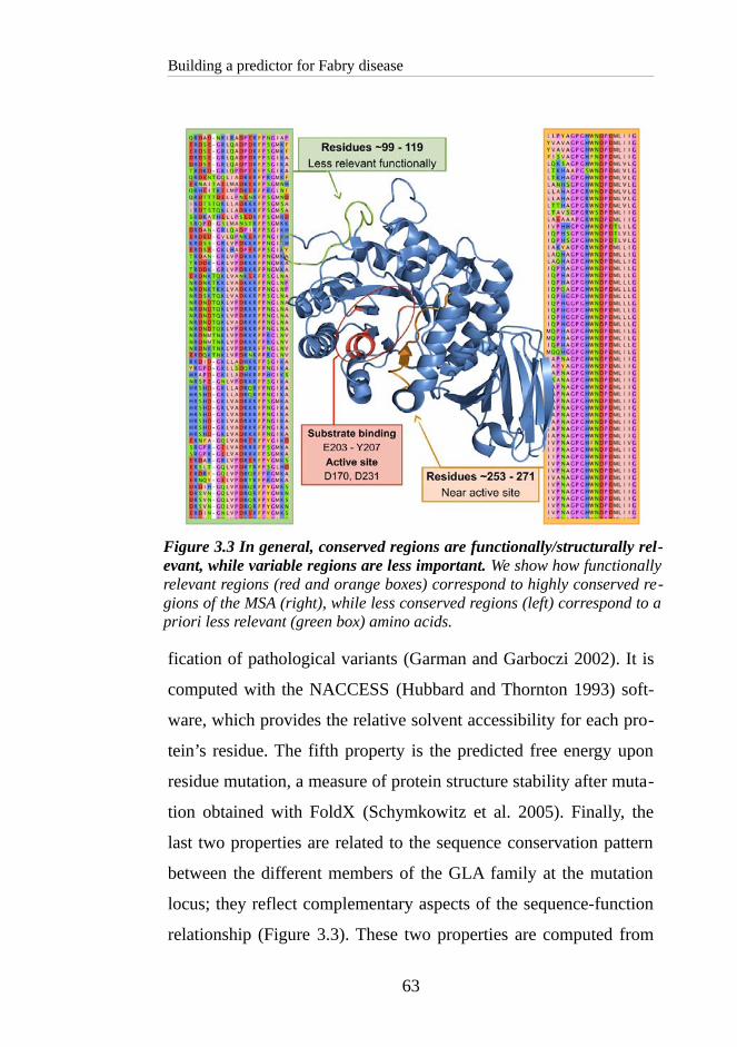
Building a predictor for Fabry disease
fication of pathological variants (Garman and Garboczi 2002). It is
computed with the NACCESS (Hubbard and Thornton 1993) soft-
ware, which provides the relative solvent accessibility for each pro-
tein’s residue. The fifth property is the predicted free energy upon
residue mutation, a measure of protein structure stability after muta-
tion obtained with FoldX (Schymkowitz et al. 2005). Finally, the
last two properties are related to the sequence conservation pattern
between the different members of the GLA family at the mutation
locus; they reflect complementary aspects of the sequence-function
relationship (Figure 3.3). These two properties are computed from
63
Figure 3.3 In general, conserved regions are functionally/structurally rel-evant, while variable regions are less important. We show how functionallyrelevant regions (red and orange boxes) correspond to highly conserved re-gions of the MSA (right), while less conserved regions (left) correspond to apriori less relevant (green box) amino acids.

Materials and Methods
the MSA for this family, at the mutation locus; they are: the Shan-
non’s entropy (Ferrer-Costa et al. 2004) and the value of the posi-
tion-specific scoring matrix (Ng and Henikoff 2001; Ferrer-Costa et
al. 2004)for the native amino acid (pssmnat). Shannon’s entropy is
equal to: −∑i
pi×log(pi) , where the index i runs over all the
amino acids at the mutation’s MSA column. It varies between 0 and
4.322, with low and high values corresponding to highly and poorly
conserved locations, respectively. The value of pssmnat is obtained
using: log(fnat,i/fnat,MSA), where fnat,i and fnat,MSA are the frequencies of
the native amino acid at the mutation locus i and in the whole align-
ment, respectively. Positive and negative values of pssmnat corres-
pond to higher and lower than expected frequencies of the native
amino acid, respectively. In an extended version of our method, V8,
we introduced an eighth property, the value of the position-specific
scoring matrix for the mutant amino acid (pssmmut). It is obtained
using the formula: log(fmut,i/ fmut,MSA), where fmut,i and fmut,MSA are the
frequencies of the mutant amino acid at the mutation site i and in
the whole alignment, respectively. When the mutant amino acid is
absent from position i of the MSA, we use 1/nseq as an estimate of
fmut,i, where nseq is the number of sequences in the alignment. Posit-
ive and negative values of pssmmut correspond to higher and lower
than expected frequencies of the mutant amino acid, respectively.
3.2.3 Building a method for the discrimination between pathological and neutral variants
We built our prediction method using the WEKA package
(v. 3.6.8) (Hall et al. 2009). WEKA is a standard in the machine
learning field that allows an easy reproducibility of our results.
64

Building a predictor for Fabry disease
Among the possible options, on the basis of previous experience
(Ferrer-Costa et al. 2004) and to reduce the chance of model overfit-
ting, we employed the simplest neural network model: a single-lay-
er neural network (Bishop 1995) with default parameters. We used
the SMOTE (Chawla et al. 2002) procedure at 600% and default
settings to correct for the imbalance (Wei and Dunbrack
2013) between pathological (332 cases) and neutral variants (48
cases).
The output of the network is a continuous score comprised
between 0 and 1. The score was transformed in a discrete prediction
using a decision threshold 0f 0.5 (default value): scores below 0.5
were assigned to neutral variants and scores above 0.5 were as-
signed to pathological variants. In addition, for each prediction, we
obtained a reliability index transforming the network output as fol-
lows (Ferrer-Costa et al. 2004): int[abs(NNout – 0.5)·20)]. The values
of this index vary continuously between 0 (lowest reliability) and 10
(highest reliability).
3.2.4 Performance estimation
Performance estimates were obtained following a standard
threefold cross-validation procedure (Hall et al. 2009; Riera et al.
2014): first, the mutation dataset was divided into three subsets;
secondly, two of them (named training set) were used to train the
method and the third (test set) to assess its performance. Next, we
repeated the second step until all three possible combinations of
subsets are used and finally, we averaged the performance values
obtained for the three test sets. Also, to take into account the effect
of distributing variants among training and test sets, the cross-valid-
65
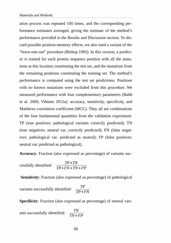
Materials and Methods
ation process was repeated 100 times, and the corresponding per-
formance estimates averaged, giving the estimate of the method’s
performance provided in the Results and Discussion section. To dis-
card possible position-memory effects, we also used a variant of the
“leave-one-out” procedure (Bishop 1995). In this version, a predict-
or is trained for each protein sequence position with all the muta-
tions at this location constituting the test set, and the mutations from
the remaining positions constituting the training set. The method’s
performance is computed using the test set predictions. Positions
with no known mutations were excluded from this procedure. We
measured performance with four complementary parameters (Baldi
et al. 2000; Vihinen 2012a): accuracy, sensitivity, specificity, and
Matthews correlation coefficient (MCC). They all are combinations
of the four fundamental quantities from the validation experiment:
TP (true positives: pathological variants correctly predicted); TN
(true negatives: neutral var. correctly predicted); FN (false negat-
ives: pathological var. predicted as neutral); FP (false positives:
neutral var. predicted as pathological).
Accuracy: Fraction (also expressed as percentage) of variants suc-
cessfully identified: TP+TN
TP+FN +TN +FP
Sensitivity: Fraction (also expressed as percentage) of pathological
variants successfully identified: TP
TP+FN
Specificity: Fraction (also expressed as percentage) of neutral vari-
ants successfully identified: TN
TN +FP
66

Building a predictor for Fabry disease
Matthews correlation coefficient (MCC), which offers a more
balance view than accuracy and is equal to:
MCC=TP·TN−FP·FN
√(TP+FN ) ·(TN +FP) ·(TP+FP) ·(TN +FN)
We give these parameters for every model derived in this
work (Tables 3.1-3.3); allowing the reader to have a complete view
of the success rate of our approach. However, for clarity purposes,
we focus our discussion on sensitivity and specificity values, since
they are broadly used in the biomedical literature, and in the MCC,
which is considered amongst the best summary measures in predic-
tion problems such as ours (Baldi et al. 2000).
3.3 Results and Discussion
3.3.1 Gauging the impact of GLA variants regarding structure and sequence properties
In this section, we compare pathological and neutral vari-
ants in terms of several properties related to mutation damage with
the purpose of obtaining a quantitative, GLA-specific understand-
ing. To this end, we considered eight of these properties (see Mater-
ials and Methods), known to contribute to the general identification
of pathological variants (Ferrer-Costa et al. 2004; Riera et al. 2014).
For each property, we compare the values of the frequency histo-
grams for our set of pathological (332 cases) and neutral (48 cases)
variants of GLA. Properties showing large differences between dis-
tributions are more explanatory and have a higher predictive value
than those for which no substantial differences are observed (Figure
3.4). In some cases we also provide sensitivity and specificity val-
67

Results and Discussion
ues, to link the descriptive analysis in this section to the subsequent
predictive power analyses, associated with the development of our
method (later section Development of the prediction method).
3.3.1.1 Structure properties
In many cases pathological variants affect protein function
by destabilizing protein structure (Wang and Moult 2003; Yue et al.
2005). As a consequence, structure properties linked to protein sta-
bility (ΔG) are routinely used to characterize pathological muta-
tions. One of these properties is residue solvent accessibility, related
to the residue solvation and packing interactions so relevant to ΔG
(Dill 1990). In addition, its simplicity allows a first interpretation of
why mutations at core residues are harder to accommodate than
those at solvent-exposed residues (Ferrer-Costa et al. 2007). In the
case of FD we found, using GLA structure (Figure 3.5A; PDB code
68
Figure 3.4 Explanation of the threshold value for single property-based predictions. For each property we obtain a cutoff value thatprovides the optimal separation between pathological and neutralvariants. This separation is optimal in the sense that if we used thiscutoff to annotate unknown mutations, the number of incorrect as-signment would be minimal.

Building a predictor for Fabry disease
3HG2), that pathological variants are more frequent than neutral
ones at buried locations (Figure 3.5B), and that the opposite is true
for exposed locations. This is in accordance with preliminary results
obtained by Garman et al. (Garman and Garboczi 2002; Garman
and Garboczi 2004), who got a similar result, but with a smaller
(206 variants) dataset. Interestingly, in our case, we also found a
substantial overlap in accessibility values between both mutation
types. This means that accessibility is not a entirely decisive para-
meter for the problem of discriminating between pathological and
neutral mutations. This is illustrated in Figure 3.5A where we can
see that some pathological mutations happen at external locations,
and for this reason, may be predicted as neutral on the sole basis of
their accessibility to solvent. This is coherent with the fact that ac-
cessibility only represents one of the energy terms contributing to
protein stability.
To overcome this limitation, we obtained ΔΔG (stability
change upon mutation) estimates for each mutation. Computing
ΔΔG is a challenging problem (Khan and Vihinen 2010) that re-
quires a detailed, quantitative knowledge of the terms that contrib-
ute to protein stability (Dill 1990) (interactions between the protein
and the solvent, between the different protein atoms, etc.) and of
their variations upon mutation. Given its interest, this problem has
been the object of active research that has led to the development of
different ΔΔG prediction programs (Khan and Vihinen 2010). These
programs describe implicitly or explicitly the interactions between
the mutated residue and its environment. For example, I-Mutant 2.0
(Capriotti et al. 2005) is a fast, SVM-based tool that uses 42 input
attributes, of which 20 are devoted to describing the amino acid
69

Results and Discussion
composition in a 9 Å sphere around the mutated residue. Dmutant
(Zhou and Zhou 2002) is based on an all-atom, knowledge-based
potential that takes into account the distance between interacting
atoms. FoldX (Schymkowitz et al. 2005) includes an empirical
force-field that models the main known contributions to ΔΔG, in-
cluding a protein solvation term, which is based on a function of the
relative solvent accessibility.
Using a large mutation set, Khan and Vihinen (Khan and
Vihinen 2010) have recently established that these three programs
70
Figure 3.5 Protein structure versus sequence conservation. (A) Fourmutation locations in yellow that are external and do not directly affectfunctional residues. (B) Relative accessibility distribution for pathological(brown) and neutral (blue) mutations. The difference between distributionsis significant (Kolmogorov–Smirnov test; p-value = 5.3 x 10 -8). (C) Distri-bution of predicted stability values upon mutation (ΔΔG) for pathologicaland neutral mutations. The difference between distributions is significant(Kolmogorov–Smirnov test; p-value = 2.2 x 10⁻¹⁶). (D) Representation of se-quence conservation logos for the four mutation locations in (A); size is re-lated to conservation degree (the larger the symbol, the more conserved theamino acid).

Building a predictor for Fabry disease
are the most reliable among a set of 11 stability predictors. For our
work, we chose FoldX because it allowed us to explore the extent to
which enriching accessibility with other physically relevant terms
improves our ability to discriminate between mutation types. When
we applied FoldX to our dataset we saw that pathological mutations
have a larger effect on protein stability than neutral mutations (Fig-
ure 3.5C), in accordance with Wang et al. (Wang and Moult 2003;
Yue et al. 2005). We also found that the computed ΔΔG values are
better than accessibility at discriminating between mutation types
(Table 3.1), confirming that improving the description of the stabil-
ity change upon mutation is generally beneficial (see also Al-
Numair and Martin 2013).
However, discrimination was still incomplete (Table 3.1),
something partly explained by the error in the estimated ΔΔG val-
ues (Khan and Vihinen 2010) and partly because protein function
and stability changes upon mutation are not always related
(Bromberg and Rost 2009). In particular, there are mutations affect-
ing protein function with no impact on stability and, therefore, we
would not be able to identify these cases even if we had error-free
ΔΔG estimates. In summary, structure properties related to protein
stability explained only part of the difference between pathological
and neutral variants in GLA.
71

Results and Discussion
Property MCC Sensitivity (%) Specificity (%) Accuracy (%)
Sequence
Blosum 62 0.21 60.0 70.8 61.32
Volume 0.10 27.7 81.3 34.5
Entropy 0.38 71.1 83.3 72.6
PSSMnat 0.34 71.1 68.8 76.1
PSSMmut 0.62 87.4 91.7 87.9
Structure
Accessibility 0.22 72.0 58.3 70.3
Stability 0.35 69.3 81.3 70.8
Table 3.1 Cross-validated prediction performance of the properties usedin this work. The first column contains the property names. Columns 2-5correspond to the four measures of performance (Matthews coefficient,MCC; Sensitivity, Specificity, and Accuracy; see Materials and Methods)for the problem of discriminating between neutral and pathological muta-tions (see also Figure 3.4). For clarity, properties are grouped into twohomogeneous classes, sequence- and structure-based.
3.3.1.2 Sequence properties
We characterized the mutations in our dataset with amino
acid-based and conservation-based properties because we know that
they are related to the effect of mutations on protein function/struc-
ture and because their discriminant power has already been tested in
other systems (Ferrer-Costa et al. 2004). We used three amino acid-
based properties. Two are related to the physico-chemical nature of
the amino acid change: van der Waals volume and Blosum62 matrix
elements. The third corresponds to functional annotations retrieved
from the UniProt (The UniProt Consortium 2014) database, provide
a straightforward, qualitative explanation for the mutation damage
caused by certain mutations (on–off switching of function) but are
72

Building a predictor for Fabry disease
limited to few residues and for this reason, will not be further con-
sidered. If we focus on the elements of the Blosum62 matrix (B62)
and on the changes in the van der Waals volume (ΔV), we see that
they both can separate pathological and neutral mutations (Figure
3.6) to a certain extent. For pathological mutations, B62 performs
better (sensitivity: 60%) than ΔV (sensitivity: 28%), in accordance
with the fact that B62 summarizes several physico-chemical proper-
ties (Ferrer-Costa et al. 2004). Neither B62 nor ΔV surpassed struc-
ture properties in the identification of pathological mutations (Table
3.1). Regarding neutral mutations, ΔV has the best specificity
(81.3%), essentially equal to that of ΔΔG (81.3%).
The situation improved when we considered conservation-
based properties (derived from the MSA for the GLA family) in-
stead of the simpler B62 and DV. We know that pathological vari-
ants tend to happen at highly conserved locations (Ferrer-Costa et
al. 2002; Yue et al. 2005). For example, in Figure 3.6D we see how
four of these variants break the residue pattern of highly conserved
columns (represented using sequence logos). MSA-based properties
provide a simple way to quantify this effect (Riera et al. 2014). In
our case we used three of them (see Materials and Methods
section): sequence variability (or Shannon entropy), frequency of
the native (pssmnat) and mutant (pssmmut) amino acids at the muta-
tion locus. We saw (Figure 3.6; Table 3.1) that the three had a dis-
criminant power comparable or superior to that of structure proper-
ties.
This was particularly true for pssmmut, which is a quantific-
ation of the discrete pattern of presence/absence of the mutant
residue, and has the best discriminant performance (Table 3.1).
73

Results and Discussion
However, this parameter has an incompletely understood
dependence on the composition of the sequence database (Bondi
1964; Ferrer-Costa et al. 2004) used to build the MSA. Because of
this, the relationship between pssmmut and function damage is un-
clear, and the results of any predictor based on its use must be con-
sidered with care.
74
Figure 3.6 Sequence-based properties. The color code is the same for thefour panels: pathological (black) and neutral (grey) variants, respectively.(A) Elements of the Blosum62 matrix; (B) changes in van der Waalsvolume; (C) Sequence variability (Shannon’s entropy) at the mutationlocus; and (D) Frequency of the native residue at the mutation locus (pos-ition-specific scoring matrix element). In all four cases, the differencebetween pathological and neutral distributions is significant (Kolmogorov–Smirnov test; p-values = 5.0 x 10⁻⁵, 0.002, 1.7 x 10⁻¹², and 7.3 x 10⁻¹⁰, re-spectively).

Building a predictor for Fabry disease
In summary, while to a certain degree all properties were
able to discriminate between pathological and neutral mutations,
none of them gave a complete separation between both mutation
types. In addition, the analyses in this section showed that for our
dataset, simple properties related to sequence conservation were
comparable to or better than structure properties at separating
pathological from neutral mutations. This is relevant because it
opened the possibility of combining them into an enhanced in silico
tool for pathogenicity prediction, going beyond the initial structure-
based analyses of mutations normally done in FD (Garman and Gar-
boczi 2002; Garman and Garboczi 2004).
3.3.2 Development of the prediction method
In the previous section, we obtained a first assessment of
the predictive ability of each of the chosen properties, finding that
they all can discriminate between both variant types (Figures 3.5
and 3.6; Table 3.1), to a certain extent. They also displayed a qualit-
atively comparable behaviour (a predominating peak per mutation
type) that suggests that low-complexity models may discriminate
between neutral and pathological variants. Taking into account both
this fact and the moderate size of our dataset, we decided to com-
bine all our properties in a simple, neural network-based prediction
method. We tried two versions of it, V7 and V8, which have seven
properties in common: solvent accessibility, FoldX free energies,
Blosum62 matrix elements, van der Waals volume, functional an-
notations, overall variability and frequency of the native residue at
the mutation site (pssmnat). The eighth property, the frequency of the
mutant residue at the mutation site (pssmmut), was only used for V8.
75

Results and Discussion
From a practical point of view, V7 represents a more conservative
approach to the prediction problem, while V8 is more permissive
because pssmmut values have an implicit database effect that is not
easy to estimate.
Method MCC Sensitiv. (%) Specif. (%) Accuracy (%) Mutation
3-fold CV
V7 0.55 88.0 79.2 86.8 332/48
V7 (R ≥5) 0.62 90.8 82.5 89.8 292/40
V8 0.65 91.6 83.3 90.5 332/48
V8 (R ≥5) 0.70 94.3 86.1 93.5 318/36
LOO CV position specific
V7 0.53 87.0 77.6 85.8 332/48
V7 (R ≥5) 0.63 91.5 79.1 89.9 284/43
V8 0.60 88.9 83.3 88.2 332/48
V8 (R ≥5) 0.70 93.3 87.2 92.6 297/39
Table 3.2 Prediction performance of the methods presented in this work.The first column contains the version names of the predictors (V7 and V8,and V7 and V8 with reliability index ≥ 5). Columns 2-5 correspond to thefour measures of performance used for discriminating between neutraland pathological variants. Column 6 corresponds to the total number ofvariants of each type used for training and testing the predictor. Vertic-ally, the table is divided into two main blocks: 3-fold CV and LOO CV po-sition specific. The first corresponds to the results of a standard 3-foldcross-validation scheme; the second to those of a "leave-one-out" proced-ure, devised to take into account position-memory effects, described in theMaterials and Methods section.
To assess the performances of V7 and V8, we followed a
threefold cross-validation scheme; the resulting values are given in
Table 3.2. For each version we also provide the results for a subset
of predictions with reliability index values between 5 and 10 (most
76

Building a predictor for Fabry disease
reliable predictions (Ferrer-Costa et al. 2004)). The first thing we
observed is that V7 and V8 have better performances (MCC: 0.55
and 0.65, respectively) than their best-constituting properties, Shan-
non’s entropy (MCC: 0.38) for V7 and pssmmut (MCC: 0.62) for V8.
For the latter, the difference is minor; however, focusing on muta-
tion type, we found that V8 is better at predicting pathological
mutations than pssmmut (sensitivity: 91.6% and 87.4%, respectively),
and the reverse is true for neutral mutations (specificity: 83.3% and
91.7%, respectively).
3.3.2.1 Discarding the existence of MSArelated biases on prediction performances
The last result suggests that part of the success rate of our
approach could be due to the presence of a position-memory effect,
arising from the use of the MSA for both building our neutral model
and computing conservation-based properties. To assess the size of
this effect, we implemented two additional analyses: one is a posi-
tion-specific version of the “leave-one-out” (LOO) protocol (Bishop
1995) (see Materials and Methods), and the other is based on the
stringent heterogeneous cross-validation protocol (Krishnan and
Westhead 2003). In the position-specific LOO, the training set was
constituted by all the variants in our dataset except those from a giv-
en sequence position, which were used for the test set. This proced-
ure was repeated for all the sequence positions in GLA, excluding
only those for which there were no known mutations. The perform-
ance was estimated on the test set predictions. We found (Table 3.2)
no remarkable differences between our original cross-validation val-
ues and those of the LOO procedure. In fact, while V7’s specificity
is marginally better for cross-validation (79.2%) than for LOO
77

Results and Discussion
(77.6%), V8’s specificity is equal for both procedures (83.3%). A
similar situation was observed when we restricted our analysis to
highly reliable predictions. This showed that there is no significant
position-memory effect in our approach and that the performance of
our method results from the predictive value of the properties
chosen.
To reinforce the previous result, we carried a simple test in
which our GLA-trained predictor was directly applied to a set of 73
human proteins with at least 50 pathological mutations described
associated to disease and 50 neutral mutations (MSA-based), to
guarantee a reasonable estimate of accuracy. This protocol is a hard
version of the already stringent heterogeneous cross-validation pro-
cedure, in which the mutations constituting the training and the test
sets must come from different proteins. Our version is harder in the
sense that only GLA mutations constitute the predictor’s training
set, while mutations from 73 other genes constitute the test set. If
our GLA-specific predictor had learned any concrete feature, arising
from the use of the same alignment to both derive neutral mutations
and compute conservation properties, it would not generalize to the
mutations of the 73 genes. We would observe a performance com-
parable to that of a random method, or worse since these genes are
unrelated to GLA and have different sequence divergence patterns.
We found that this was not the case, and that when we applied V7
and V8 to the 73 genes, we obtained specificities (58% ± 17% and
84% ± 11%, respectively) that are significantly above 50% (Stu-
dent’s T-test p-values = 6 x 10⁻⁵ and ~10-16, respectively), the spe-
cificity of a random method. Also, we computed the corresponding
MCCs, to verify that the overall predictive behaviour was not lost
78

Building a predictor for Fabry disease
and that disease mutations were also identified. The average MCC
for V7 and V8 were 0.50 ± 0.16 and 0.69 ± 0.16 (both T-test p-val-
ues = 10-16), respectively, indicating that this was indeed the case.
Overall, these and the LOO results confirmed that any position-
memory effect in our performance measures, if present, must be
small.
3.3.3 Comparison with other predictors
We then compared V7 and V8 with general prediction
methods (Table 3.3; performances for all methods are obtained only
on the Fabry mutation set). For this comparison, we used our cross-
validated performance figures, since the general methods utilized
(SIFT, PolyPhen-2, and Condel) were not trained taking into ac-
count position-specific effects. Both versions of our predictor have
(V7, MCC: 0.55; V8, MCC: 0.65) similar or better performance
than SIFT and Condel2 (MCC: 0.55 and 0.52, respectively) and V8
also performed better than PolyPhen-2 (MCC: 0.61). For the last
comparison, it has to be noted that the difference between both
methods is consequence of the higher specificity of V8 (83.3%) rel-
ative to PolyPhen-2 (72.9%) since their sensitivities are comparable
(91.6% vs. 93.1%, for V8 and PolyPhen-2, respectively).
2 Note: Condel results were obtained with the first version of the method; atthat present time, the authors were in the process of replacing it by an updatedversion, we opted for using the first, stable version.
79

Results and Discussion
Method MCC Sensit. (%) Specif. (%) Accuracy (%) Mutations
V7 0.55 88.0 79.2 86.8 332/48
V7 (R ≥5) 0.62 90.8 82.5 89.8 292/40
V8 0.65 91.6 83.3 90.5 332/48
V8 (R ≥5) 0.70 94.3 86.1 93.5 318/36
PPH2-Div 0.61 93.1 72.9 90.5 332/48
PPH2-Var 0.58 88.9 81.3 87.9 332/48
SIFT 0.55 84.0 87.5 84.5 332/48
Condel 0.52 82.8 86.4 83.2 322/44
Table 3.3 Comparison of the cross-validated performance between the gene-specific method presented here and general methods (PolyPhen-2 (PPH2),SIFT, Condel). Column 1 is the method's name; columns 2-5 correspond tothe four performance measures (Matthews correlation coefficient, MCC;Sensitivity, Specificity, and Accuracy; see Materials and Methods) usedhere; column 6 provides the number of predictions made by the method (themaximum numbers are: 332 pathological and 48 neutral variants).
A qualitative explanation of the performance differences
between our predictor and the other methods can be obtained when
comparing the information in which they are based. In the case of
SIFT, we know that this program is based on the use of sequence in-
formation only (Ng and Henikoff 2003), while we also used struc-
ture information, which by itself already had a substantial predictive
power (Table 3.1). This would explain our better performance. In
the case of PolyPhen-2 (Adzhubei et al. 2010), which uses a com-
bination of properties comparable to that in our predictor, the per-
formance differences were smaller. Finally, we couldn’t really ad-
vance an explanation for the differences observed with Condel, be-
cause it is a consensus method that combines the scores of different
80
Building a predictor for Fabry disease
programs (including SIFT and PolyPhen-2, in the version utilized),
which use themselves different information types.
Looking at the results from the point of view of the muta-
tion type (Table 3.2), all the versions of our method had sensitivity
higher than specificity, meaning that they are better at predicting
pathological than neutral variants. This trend was also observed for
PolyPhen-2, while the opposite was true for SIFT and Condel. This
reinforces the idea that when scoring mutations it is advisable, par-
ticularly in a clinical setting, to combine the predictions from differ-
ent methods (Ohanian et al. 2012; Richards et al. 2015).
3.3.4 Using prediction reliability to enhance success rate
As mentioned before, for a given mutation, the difference
between its score (the output of the neural network) and the de-
cision threshold (which is 0.5), can be used to obtain a discrete in-
dex (see Materials and Methods). This index varies between 0 and
10, and is related to the reliability of the prediction: low values cor-
respond to less reliable predictions than high values. This informa-
tion can help to weight bioinformatics evidence, particularly in clin-
ical settings where it is combined with data from other sources
(Sunyaev 2012).
We divided the index range into two parts and defined as
high-quality predictions those with reliability index between 5 and
10. This condition was fulfilled by 87% (for V7) and 93% (for V8)
of the variants in the original dataset. The prediction performance of
these high-quality predictions was indeed better (Table 3.2). For ex-
ample, MCC values went from 0.55 to 0.62, for V7, and 0.65 to
81
Results and Discussion
0.70 for V8. In both cases also, MCC values were better than those
of the general methods. Overall, this showed that the reliability in-
dex is a valuable tool to help judge the validity of the predictions.
3.3.5 Independent validation of the FDspecific predictor
The previous performance figures were cross-validated es-
timates, obtained from the original set of 332 pathological and 48
neutral variants. While developing our method, an update of the
Fabry database (Sakuraba 2012) with 65 new pathological muta-
tions became available. Subsequently, at the moment of writing this
chapter, 106 new mutations have been added to the Fabry database,
22 of them with a known Fabry phenotype associated. We used
these two collections (65 and 22 cases) as validation sets for our
predictor. The sensitivities for the different versions of our method
in the first set were: 90.8% and 95.1%, for V7 and V7 (reliab. ≥ 5,
61 predicted mutations), respectively; 89.2% and 98.2%, for V8 and
V8 (reliab. ≥ 5, 57 predicted mutations), respectively. For the
second set, sensitivities were 94.7% for V7 (all predictions with re-
liab. ≥ 5), and 94.4% for V8 (reliab. ≥ 5, 20 predicted mutations).
This confirmed that the predictive ability of our method for Fabry
pathological variants is in the neighbourhood of 90-95%. The cor-
responding sensitivities for SIFT and PolyPhen-2 were 73.8% and
87.7% for the first set, and 84.2% and 94.7% for the second set.
Overall, they are slightly lower than our performances but consist-
ent with the values listed in Table 3.3.
In summary, we see that our Fabry-specific method has a
competitive prediction performance when compared with general
82

Building a predictor for Fabry disease
methods, even in its more conservative form (V7); this is of value,
given its simplicity. Our method has been trained and validated
against manually curated variants and can be easily updated as new
variants are described, or enriched and re-trained with clinical para-
meters from patient records, such as GLA activity levels or symp-
toms. We want to note, however, that our method is not meant to re-
place general methods in the case of FD; rather, it is conceived to be
used together with them, to support the decision-making process un-
derlying its diagnosis.
3.4 Conclusion
An unknown percentage of Fabry disease patients, particu-
larly females, do not benefit in time from the available therapies be-
cause they are not diagnosed until the disease is too advanced. Iden-
tification, through GLA sequencing, of pathological variants is a
good option to address this problem if the variant found has already
been described as causative. However, this strategy fails when the
variant identified is novel; in this case, we need additional tools to
verify its functional effect. Here, we address this problem develop-
ing and validating an automated method to predict the pathogenic
effect of missense variants in GLA. To do so, we first characterized
GLA pathological variants in terms of a small set of properties that
allowed their separation from neutral variants and, second, we com-
bined these properties in a Fabry-specific method. Our results show
that MSA-based properties have a higher prediction power than
structure-based properties (Table 3.1); we also find that the method
based on the combination of both property types has a prediction
performance equal or better than that of available general ap-
83

Conclusion
proaches (PolyPhen-2, SIFT, and Condel). In addition, for each pre-
diction we obtained a simple reliability index that allows the identi-
fication of high-quality predictions. We believe that this tool will al-
low to advance in the analysis of unknown variants of GLA and
contribute to the diagnosis of their carriers, a process in which it can
be used in combination with other available in silico predictors.
84


4 PROTEINSPECIFIC
AND GENERAL
PATHOGENICITY
PREDICTORS

The results presented in this chapter have been recently ac-
cepted in Human Mutation (Riera C, Padilla N, de la Cruz X. The
complementarity between protein-specific and general pathogeni-
city predictors for amino acid substitutions.) and are now in press.

Protein-specific and general pathogenicity predictors
4.1 Why proteinspecific predictors?
In the previous chapters, we have already introduced the
idea that using protein-specific pathogenicity tools is a promising
alternative to breaking the present bottleneck in prediction perform-
ance. The rationale behind is that use of specific models allows re-
searchers to capture some of the unique characteristics of genes; in
particular, those for which we do not yet have a general, quantitat-
ively precise theory. Like, for example, the residues directly or in-
directly involved in protein function, those preventing aggregation,
etc.
The idea of using specific information for predictor devel-
opment has been explored in a small number of studies, where spe-
cific predictors were obtained by training them only with variants
from the protein(s) of interest. This is the case of the predictor for
the Mismatch Repair genes, trained using a set of 168 functionally-
tested variants for four genes (Ali et al. 2012); or KinMut-2, a tool
for the interpretation of kinase variants using a disease set consti-
tuted by 1,021 variants from 84 kinases (Izarzugaza et al. 2012); or
several others (Santibáñez-Koref et al. 2003; Karchin et al. 2007;
Torkamani and Schork 2007; Jordan et al. 2011; Stead et al. 2011;
Crockett et al. 2012; Masica et al. 2012; Hamasaki-Katagiri et al.
2013; Li et al. 2013b; Fechter and Porollo 2014; Leong et al. 2015;
Niroula and Vihinen 2015; Adebali et al. 2016). Although they have
shown a good success, a careful look at these papers shows specific
information is not always enough to improve the performance of
general methods, like SIFT or PolyPhen-2. This is patent in the case
88

Protein-specific and general pathogenicity predictors
for the F8-specific predictor (Hamasaki-Katagiri et al. 2013) where
the authors reach performances slightly below those of PolyPhen-2.
This deviation from the expected behaviour can be of a purely tech-
nical origin, and due to the fact that protein-specific predictors are
trained with smaller (between one and two orders of magnitude)
datasets than general predictors, since only variants from the target
protein are considered. The consequent reduction in the complexity
range of the predictive models (Bishop 1995) can explain the exist-
ence of poorer predictions. In few words, predictors may fail be-
cause variant impact is not properly represented. The second reason
is of a more fundamental nature, and results from the fact when a
general method is really good at annotating the variants of a given
protein, the range for improvement left to protein-specific tools may
be very reduced. In the limit, if the general method was perfect, no
improvement whatsoever could be obtained.
In this chapter, we use the experience gained during the de-
velopment of the Fabry-specific predictor (Chapter 3) to go one step
further and characterize the relationship between protein-specific
predictors (PSP) and general methods (GM). To this end, we gener-
ated a larger number of independent PSP and compared them to
standard, state-of-the-art general methods. These general methods
covered a broad range of approaches to the prediction problem, and
were represented by SIFT (Kumar et al. 2009), PolyPhen-2
(Adzhubei et al. 2010), PON-P2 (Niroula et al. 2015), Mutation-
Taster2 (Schwarz et al. 2010), CADD (Kircher et al. 2014) and a
simple in-house general predictor.
In the following pages, we analyse the relationship
between these two approaches. We also describe how the size of the
89

Why protein-specific predictors?
improvement provided by PSP depends on GM performance, a crit-
ical issue if we have to decide whether to use or develop PSP. Fi-
nally, we discuss how the observed complementarity between ap-
proaches can lead to increased success rates in the pathogenicity
prediction process, when working within the limits marked by the
ACMG/AMP (American College of Medical Genetics and Genom-
ics/Association for Molecular Pathology) rule for the in silico inter-
pretation of sequence variants (Richards et al. 2015).
4.2 Materials and Methods
The goal of this work is to compare PSP and GM and
check the degree to which they complement each other. To this end,
we developed 83 in-house predictors, of which 82 PSP and one GM,
which we called ihGM. For all of them, we followed the same,
standard protocol (Riera et al. 2014) (Figure 4.1). This protocol is
divided into three main steps: (i) obtention of a dataset of patholo-
gical and neutral variants, (ii) characterization of variants with sev-
eral properties, and (iii) build a neural network model for variant
prediction and estimate its performance (success rate).
4.2.1 The variant datasets
The development of the pathogenicity predictors required a
set of pathological and one of neutral variants. For the PSP, these
sets contained single amino acid variants affecting only the protein
of interest. A minimum of 50 cases of each kind was required, to en-
sure the subsequent viability of the model-building step; otherwise,
the protein was discarded. For ihGM, we pooled all the collected
90

Protein-specific and general pathogenicity predictors
variants to obtain one pathological and one neutral dataset. Below
we explain how we built the protein-specific datasets.
For every protein in our work, pathological and neutral
variants were collected following commonly used protocols (Riera
et al. 2014). Pathological variants were retrieved from UniProt (The
UniProt Consortium 2014) and corresponded to those single amino
acid replacements labelled as "Disease" in Humsavar (version
2015_02, 04-Feb-2015).
For neutral variants, there are two main possible options
(Riera et al. 2014): homology-based and population-based. We
chose the former because it gave more proteins with > 50 neutral
variants than the population-based model (which gave only one pro-
tein fulfilling this condition). The homology-based model is charac-
terized by the fact that neutral variants are obtained from a multiple
sequence alignment (MSA) for the protein family. They correspond
91
Figure 4.1 Diagram of the procedure followed to build the protein-specif-ic (PSP) and general (GM) methods. The shaded boxes highlight the mainsteps: (i) building the set of pathological and neutral variants; (ii) charac-terization of the variants in terms of sequence and conservation properties;(iii) obtention and performance estimation of the predictors.

Materials and Methods
to those sequence deviations from the human representative ob-
served in close homologs (sequences from other species ≥ 95%
identical to the human one) (Ferrer-Costa et al. 2004). This is the
same approach we followed in the work of Fabry disease (see sec-
tion 3.2.1 for details). At the end of this process, we had a total of
82 proteins (Table 7.2, Appendix 2) with a median of 74.5 (values
comprised between 50 and 472) pathological and 134 (values com-
prised between 50 and 1271) neutral variants. Each of these proteins
was used to develop one of the PSP. As mentioned before, to build
ihGM, we pooled all the variants. This gave a total of 8020 patholo-
gical and 19353 neutral variants.
4.2.2 Characterization of variants in terms of discriminant properties
We used the same six properties for all our models (PSP
and ihGM), which were chosen on the basis of the work with Fabry
disease. The first three account for some of the physico-chemical
differences between the native and mutant amino acids: the differ-
ence in Van der Waals volumes (Bondi 1964) and hydrophobicities
(Fauchère and Pliska 1983) and the corresponding element of the
Blosum62 matrix (Henikoff and Henikoff 1992). The fourth prop-
erty is a binary variable that summarizes any information available
on the functional or structural role of the native residue. It is based
on UniProt annotations, and is equal to “1” when the native residue
has any of these annotations: 'initiator methionine', 'signal peptide',
'propeptide', 'transmembrane region', 'calcium-binding region', 'zinc
finger region', 'DNA-binding region', 'nucleotide phosphate-binding
region', 'region of interest', 'active site', 'metal ion-binding site',
92

Protein-specific and general pathogenicity predictors
'binding site', 'site', 'modified residue', 'lipid moiety-binding region',
'glycosylation site', 'disulfide bond', 'cross-link' and 'short sequence
motif'. Otherwise, the value is 0. Finally, we used two properties re-
lated to the sequence conservation pattern at the variant locus, com-
puted from the MSA of the protein family. The first was Shannon's
entropy (Ferrer-Costa et al. 2004); it is equal to −∑i
p i×log( p i)
where the index i runs over all the amino acids at the variant's MSA
column. The second was the value of the position-specific scoring
matrix (Ng and Henikoff 2001) for the native amino acid, pssmnat,
which is equal to log(fnat,i/fnat,MSA), where fnat,i and fnat,MSA are the fre-
quencies of the native amino acid at the variant locus i and in the
whole alignment, respectively. Positive and negative values of
pssmnat correspond to higher and lower than expected frequencies of
the human native amino acid, respectively.
4.2.3 Building the predictor method
We built all our predictors using WEKA (v3.6.8) (Hall et
al. 2009), a standard software in the machine learning field. We em-
ployed the simplest neural network model: a single-layer perceptron
(default settings). This model was chosen because of its low number
of parameters, which makes it appropriate to obtain PSP, given the
relatively small number of available variants per protein.
In the training, we applied SMOTE (Chawla et al. 2002) to
correct the imbalance between the number of neutral and patholo-
gical variants (Wei and Dunbrack 2013; Riera et al. 2015). To com-
pare the effect of oversampling against other approaches such as un-
dersampling, we also repeated the training applying an under-
93

Materials and Methods
sampling approach using the SpreadSubSample filter from WEKA
and adjusting maxCount to the number of variants of the smallest
population, usually, pathological variants.
For a given variant, the resulting predictor produces a con-
tinuous score comprised between 0 and 1. If its value is below 0.5
the variant will be labelled as neutral; otherwise, it will be labelled
as pathological.
4.2.4 Performance assessment
We separately applied the leave-one-out cross-validation
(LOO CV) procedure to each predictor, to estimate its performance.
In this procedure, (i) one variant is excluded from the variant data-
set, (ii) the remaining variants are used to train a predictor, (iii) this
predictor is applied to the omitted variant, (iv) steps (i)-(iii) are re-
peated for all the variants in the dataset, and (v) an estimate of the
predictor’s performance is obtained from the results in the omitted
variants. We measured performance with four parameters com-
monly used in the description of bioinformatics predictors (Baldi et
al. 2000; Vihinen 2012a): sensitivity, specificity, accuracy and Mat-
thews correlation coefficient (MCC). These parameters have already
been described in Chapter 3 (see section 3.2.4). For simplicity, our
analyses focus on the values of the MCC, but comparable results are
obtained using accuracy.
4.2.5 External prediction methods
For comparison purposes, PolyPhen-2 (Adzhubei et al.
2010), SIFT (Kumar et al. 2009), PON-P2 (Niroula et al. 2015),
MutationTaster2 (Schwarz et al. 2010) and CADD (Kircher et al.
94
Protein-specific and general pathogenicity predictors
2014) predictions were obtained for all the variants in our datasets.
PolyPhen-2 was executed locally with default parameters, using the
standalone source code v2.2.2, retrieved from their website. SIFT
(sift.jcvi.org) and PON-P2 (structure.bmc.lu.se/PON-P2) predic-
tions were generated using the web versions of these programs.
MutationTaster2 and CADD predictions were obtained from AN-
NOVAR software tool (Wang et al. 2010). Neither Mutation-Taster2
nor CADD gave predictions for amino acid substitutions resulting
from more than one nucleotide change; this resulted in a smaller
coverage for these methods.
4.3 Results and Discussion
A growing amount of evidence indicates that protein-spe-
cific approaches are a good option to progress beyond the perform-
ance of GM in the prediction of pathogenic variants (Riera et al.
2014). On the other side, a priori reasoning indicates that this may
not always be the case. Our goal is to clarify this situation, charac-
terizing the complementarity between these two approaches from a
predictive point of view, showing whether and to which extent they
outperform each other.
This section is divided into three parts that correspond to
the parts in which we have broken down the problem. First, we de-
scribed the differences between proteins for GM predictors, using a
set of 82 proteins. Secondly, for each of these 82 proteins, we ob-
tained a PSP and estimated its performance. Third, we compared
PSP and GM to see if and how they outperform each other. We first
address this problem in the case when the only difference between
methods is the training set (ihGM: a pool of variants from different
95

Results and Discussion
proteins; PSP: only variants from the protein of interest). Then, we
relax this condition and repeat the analysis, this time comparing the
performance of five GM predictors with that of PSP.
4.3.1 The performance of GM predictors varies across proteins
We applied six general predictors (SIFT, PolyPhen-2,
PON-P2, MutationTaster2, CADD, and ihGM) to the variants in our
dataset. In Figure 4.2, I show the results broken down per protein.
We see that, for each of the six methods, performance varies
between proteins. There are clear differences between the most ex-
treme cases, e.g. between COL3A1 or COL1A2 for which all GM
give very good predictions, and ACTA1 or NF1 for which all GM
give near-random predictions. In general, the MCC cover a wide in-
terval (Figure 4.3): [0.0, 0.97] for SIFT, [0.13, 0.94] for PolyPhen-2,
[0.0, 1.0] for PON-P2, [-0.26, 1.0] for MutTaster2, [-0.58, 0.95] for
CADD and [0.20, 0.96] for ihGM. Most of the values are concen-
trated between 0 (random method) and 1 (perfect method), and the
few negative values observed correspond to cases for which the
method had low coverage for a given protein. Comparable results
are obtained for accuracy values, which cover broad intervals:
[0.51, 0.99] for SIFT, [0.55, 0.98] for PolyPhen-2, [0.13, 1] for
PON-P2, [0.08, 1.0] for MutationTaster2, [0.25, 1] for CADD and
[0.48, 0.99] for ihGM. Most values comprise between 0.5 (random
method) and 1 (perfect method), and the few values below 0.5
mostly correspond to cases for which a GM had low coverage for
the given protein.
96

Figure 4.2 Performance of general methods on a per protein basis. In the radar chart, we show the performance of the sixgeneral methods used: ihGM (the in-house general predictor), SIFT, PolyPhen-2, PON-P2, CADD and MutationTaster2. Per-formance is measured with the Matthews correlation coefficient (MCC), and is computed separately for each protein andmethod. The black line represents the average performance for each protein and was used to sort them. The scatter plot to theright is an amplified view of the region boxed in the radar chart and serves to give more detail on the protein-level variabilityof GMs.

Results and Discussion
In summary, by looking at the prediction results on a pro-
tein-per-protein basis, we see that the performances of standard GM
and ihGM fluctuate between proteins. This is in agreement with
data from the literature, e.g. for PolyPhen-2 researchers have found
MCC values of 0.44 for voltage-gated potassium channels (Stead et
al. 2011), 0.55 for NPC1 (Adebali et al. 2016) or 0.61 for alpha-
galactosidase A (Riera et al. 2015).
98
Figure 4.3 Variability in the performance of general methods. Boxplotof MCC values for each of the 82 proteins, grouped by general method.

Protein-specific and general pathogenicity predictors
4.3.2 Obtention and characterization of protein specific predictors (PSP)
For each of the 82 proteins, we developed a PSP following
the protocol detailed in the Materials and Methods and then estim-
ated its performance. Figure 4.4 shows that, on the average, the per-
formances of these PSP are better than random (p-value < 2.2 x 10⁻¹⁶
with the one sample t-test for each performance parameter): Accur-
acy (0.85 ± 0.07), MCC (0.66 ± 0.15), sensitivity (0.85 ± 0.06) and
99
Figure 4.4 Performance of the 82 protein-specific predictors (PSP). Weshow the results for four standard parameters: accuracy (A), Matthews cor-relation coefficient (B), sensitivity (C) and specificity (D). As a reference,the vertical dashed lines locates the values of these parameters for a ran-dom predictor. The y-axis corresponds to the frequency (number of pro-teins). In (B) we indicate with arrows the location of MYO7A and that of theCOL family, both mentioned in the text.

Results and Discussion
specificity (0.85 ± 0.07). The variation range for accuracy went
from 0.70 to 0.99 and for MCC between 0.19 to 0.98.
We observed no differences in the performance between
the undersampling and the oversampling (SMOTE) approach (Fig-
ure 4.5). For 18 PSP for which we could find a comparable method
in the literature (Table 4.1) we saw no statistically significant per-
formance differences between our PSP and those from the other re-
searches: p-values of 0.79 and 0.67 for the MCC (9 cases) and the
sensitivity (9 cases) comparisons, respectively. That is, our PSP
constitutes a good representation of the protein-specific approach
because they were derived following a unified protocol (Figure 4.1)
and gave results consistent with those obtained by other colleagues
in the field.
100
Figure 4.5 Comparison between oversampling and under-sampling approaches. Comparison between the performancesobtained (measured with MCC) when the strategies of over-sampling (SMOTE) (y-axis) and undersampling (x-axis) are ap-plied during the training of the prediction methods (Pearson'scorrelation 0.975, p-value < 2.2 x 10⁻¹⁶).

Protein-specific and general pathogenicity predictors
Protein Type Parameter PSPPSP
LiteratureReference
KCNH2 Protein MCC 0.645 0.620 Leong et al. 2015
SCN5 Protein MCC 0.560 0.320 Leong et al. 2015
ABCC8 Protein MCC 0.454 0.436 Li et al. 2014
NPC1 Protein MCC 0.540 0.590 Adebali et al. 2016
CYBB +
CYP21A2Family MCC 0.680 0.700
Fechter and Porollo
2014
KCNH2 +
SCN5AFamily MCC 0.600 0.700 Stead et al. 2011
MLH1 +
MSH2Family MCC 0.580 0.770 Ali et al. 2012
BTK +
FGFR1/2
+ RET
Family MCC 0.590 0.600Izarzugaza et al.
2012
BTK +
FGFR1/2
+ RET
Family MCC 0.590 0.600Torkamani and
Schork 2007
CFTR Protein Sensitivity 84.2 78.5 Crockett et al. 2012
COL4A5 Protein Sensitivity 94.5 90.0 Crockett et al. 2012
NF1 Protein Sensitivity 77.4 96.0 Crockett et al. 2012
PAH Protein Sensitivity 81.6 92.5 Crockett et al. 2012
RET Protein Sensitivity 84.0 94.0 Crockett et al. 2012
F8C Protein Sensitivity 96.0 74.8Hamasaki-Katagiri et
al. 2013
CFTR Protein Sensitivity 84.2 74.0 Masica et al. 2012
MYH7 Family Sensitivity 83.0 94.0 Jordan et al. 2011
101

Results and Discussion
Protein Type Parameter PSPPSP
LiteratureReference
MLH1 +
MSH2/6 +
PMS2
Family Sensitivity 80.0 88.0Niroula and Vihinen
2015
Table 4.1 Comparison between our PSP and equivalent PSP found in theliterature. Under the Specificity column we indicate whether the latterwas trained using single-protein or protein family data. Two performancemeasures are listed, depending on their availability: MCC and sensitivity.
At a particular level, we observe that PSP performances
may differ substantially between proteins (Figure 4.4). In fact, some
predictors have high success rates, like those corresponding to the
members of the collagen family (COL1A1, COL1A2, COL2A1,
COL3A1, COL4A4, COL7A1) (Figure 4.4B), with an average
MCC of 0.86 ± 0.11. On the opposite side, we find cases such as
that of MYO7A, which has a really low MCC, 0.19.
The variability in the performance of PSP depends on di-
verse aspects of the prediction problem, like composition and size
of the variant datasets, and/or nature of the variant properties. For
example, an unequal number of neutral and pathological variants in
the sample, or imbalance, is known to affect predictor performance
(Wei and Dunbrack 2013). Although a correction for this effect was
applied, a few proteins with highly different numbers of neutral and
pathological variants gave modestly performing PSP (Figure 4.6A).
This is the case for the MYO7A predictor, derived from a set of
1186 and 50 neutral and pathological variants (a ratio of ~24:1), re-
spectively, and giving an MCC of 0.19. In general, the imbalance
was more frequent in big proteins, because they usually contribute
more neutral variants.
102
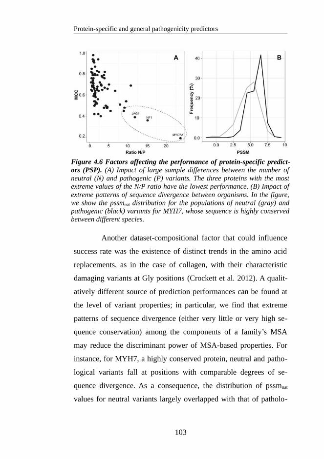
Protein-specific and general pathogenicity predictors
Another dataset-compositional factor that could influence
success rate was the existence of distinct trends in the amino acid
replacements, as in the case of collagen, with their characteristic
damaging variants at Gly positions (Crockett et al. 2012). A qualit-
atively different source of prediction performances can be found at
the level of variant properties; in particular, we find that extreme
patterns of sequence divergence (either very little or very high se-
quence conservation) among the components of a family’s MSA
may reduce the discriminant power of MSA-based properties. For
instance, for MYH7, a highly conserved protein, neutral and patho-
logical variants fall at positions with comparable degrees of se-
quence divergence. As a consequence, the distribution of pssmnat
values for neutral variants largely overlapped with that of patholo-
103
Figure 4.6 Factors affecting the performance of protein-specific predict-ors (PSP). (A) Impact of large sample differences between the number ofneutral (N) and pathogenic (P) variants. The three proteins with the mostextreme values of the N/P ratio have the lowest performance. (B) Impact ofextreme patterns of sequence divergence between organisms. In the figure,we show the pssmnat distribution for the populations of neutral (gray) andpathogenic (black) variants for MYH7, whose sequence is highly conservedbetween different species.

Results and Discussion
gical variants (Figure 4.6B), dramatically reducing the discriminant
power of this property.
In summary, for the 82 proteins used in this work, we have
built a set of PSP that can identify pathological variants with a suc-
cess rate above random, although their performance varies between
proteins.
4.3.3 The complementarity between PSP and GM
We also explored the relationship between GM and PSP
and, concretely, the extent to which these two approaches are com-
plementary. The results are divided into two blocks. The first one
corresponds to the PSP-ihGM comparison, where any observed fea-
ture originates from the use of specific vs. general information,
since the methods are otherwise equal. This procedure excludes ef-
fects arising from differences in the machine learning tools, in the
multiple-sequence aligners, in the variant attributes, etc. The second
block of results corresponds to five comparisons (PSP-SIFT, PSP-
PolyPhen-2, PSP-PON-P2, PSP-MutationTaster2, PSP-CADD),
where we studied if complementarity was also observed when con-
sidering standard methods. The five methods covered different ap-
proaches to the pathogenicity prediction problem and are broadly
used (Katsonis et al. 2014). To finish this section we also describe
an alternative to enhance the prediction performance by combining
both types of methods, an approach of clinical value since it is com-
pliant with the ACMG/AMP guidelines (Richards et al. 2015).
104

Protein-specific and general pathogenicity predictors
4.3.3.1 PSP vs. the inhouse general method (ihGM)
In Sections 4.3.1-4.3.2 we found that the performances of
ihGM and PSP varied between proteins. Here, I compare these two
approaches, checking whether PSP systematically outperforms
ihGM or whether they are complementary, that is, that one approach
is not always preferable to the other.
An overall comparison showed that out of 82 proteins, PSP
outperformed ihGM in 51 cases (62%), and the opposite happened
in 31 cases (38%) (Table 4.2). The trend was significant (p-value =
0.018, Binomial test), but the moderate difference indicated a scen-
ario of complementarity, in which PSP tended to be better than
ihGM, but not systematically. The variability observed for GM in
Figure 4.2 suggests that PSP outperforms ihGM mostly when the
performance of the latter is low. However, we found that this was
not the case: when sorting our proteins according to how ihGM
fares for them, we saw that PSP may surpass ihGM regardless of the
latter's performance (Figure 4.7A). Another apparent feature is a
clear variability in the amount by which a PSP can improve ihGM.
In Figure 4.7A, we see this effect in action for absolute values, and
in Figure 4.7B for relative values. The improvement displayed by
PSP becomes smaller as ihGM gets closer to a 100% perfect meth-
od. The opposite is the case for proteins with low ihGM success
rates; for them, PSP could be very successful. For example, for
SCN1A the MCC goes from 0.46 for ihGM to 0.78 for its PSP, a
70% improvement. However, there were also cases for which both
ihGM and PSP had poor performances, like MYO7A for which the
MCC were 0.20 and 0.19, respectively.
105

Results and Discussion
In summary, we found that PSP and ihGM predictors com-
plemented each other, with a trend for PSP to outperform ihGM.
Also, we saw that the size of the improvement shown by PSP de-
pends on ihGM success rate, with a certain variability degree.
106
Figure 4.7 Comparison between PSP and an equivalentihGM on a per protein basis. (A) For each protein in ourdataset, we represent the MCC of its PSP (black) and ihGM(gray). To facilitate the comparison we sorted the proteins ac-cording to their ihGM MCC values. (B) Relative differencebetween the MCC of PSP and ihGM as a function of the ihGMMCC.

Protein-specific and general pathogenicity predictors
IhGM SIFT PPH-2 CADD PON-P2MutTaster
PSP (%) 51
(62.2)
68
(82.9)
40 (48.8) 44 (53.7) 18 (22.0) 70 (85.4)
Av.Cover
(SD)
1.0
(0.0)
0.98
(0.16)
0.99
(0.06)
0.75
(0.29)
0.58
(0.14)
0.75 (0.29)
Table 4.2 Number of proteins for which the performance of their PSP isabove that of one or more GM (ihGM, SIFT, PPH-2, CADD, PON-P2,MutationTaster2). First line: absolute number and percentage relative tothe total of 82 proteins. Second line: average coverage of the GM andstandard deviation (in parentheses).
4.3.3.2 PSP vs. standard general methods
We compared PSP against five general methods: SIFT,
PolyPhen-2, PON-P2, MutationTaster2 and CADD. The resulting
107
Figure 4.8 Combination of protein-specific predictors (PSP) andPolyPhen-2 under the ACMG/AMP guidelines for a set of 18proteins with 100 or more variants of each type. The radar plotshows the predictive performance (MCC) that results from apply-ing the ACMG/AMP rule (black) for combining in silico predict-ors, thus indicating that application of this rule results in betterpathogenicity predictions.

Results and Discussion
overall view (Table 4.2) was similar to that found in the previous
section: in no case, one method always outperformed the other, al-
though some trends were detected. First, the differences observed
for the PSP-PolyPhen-2 and PSP-CADD comparisons were not sig-
nificant: PolyPhen-2 outperformed PSP for 40 proteins (p-value =
0.63, Binomial test), and PSP outperformed CADD for 44 proteins
(p-value = 0.29, Bin. test). Second, for the PSP-SIFT and PSP-
MutationTaster2 comparisons, PSP showed a significant trend to
surpass the GM in 68 proteins (p-value < 10-6, Bin. test) and 70 pro-
teins (p-value < 10-6 , Bin. test), respectively. And third, for the PSP-
PON-P2 comparison, the opposite was the case, with PON-P2 sur-
passing PSP for 70 proteins (p-value < 10-6, Bin. test). This case was
in itself interesting since it showed that GM can identify a subset of
variants (PON-P2 coverage is 58%) for which the predictions are
better that those of PSP. As in Section 4.3.3.1, we obtained a richer
view of the complementarity between PSP and GM using a per pro-
tein representation of the results, sorted according to the perform-
ance of each GM (Figures 4.9A-E). The complementarity pattern
moved between two scenarios; the first, which corresponds to the
PSP-PolyPhen-2 and PSP-CADD comparisons (4.9B and D), is
similar to that found for the PSP-ihGM comparison (Figure 4.7):
PSP and GM outperformed each other across the performance range
of GM. In the second scenario, PSP outperformed GM mostly for
those proteins with low GM performance, like in the PSP-PONP2
comparison (Figure 4.9C).
The two remaining cases (PSP-SIFT and PSP-MutTaster2,
Figure 4.9A and E) were less clear, because there are not many pro-
108

Protein-specific and general pathogenicity predictors
teins for which the GM outperformed PSP, and they did not define a
clear trend.
109
Figure 4.9 Comparison between protein-specific predictors (PSP) and fivestandard general methods (GM). (A) For each protein in our dataset, we rep-resent the MCC of its PSP (black dots) and that of SIFT (inverted triangles).Proteins are sorted according to their MCC values for SIFT (from left to rightproteins have increasingly high MCC). Figures B-E are equivalent to (A), butfor PolyPhen-2, PON-P2, CADD, and MutationTaster2, respectively; throughall of them PSP data are consistently represented with black dots. (F) Cover-age of the five GM.

Results and Discussion
Finally, if we focus on the amount by which a PSP could
improve a GM, we see the same trend as before: this amount gets
smaller as the proteins display higher GM performances. On the op-
posite side, when the GM performance dropped, PSP could display
larger success rates, for example, for COL7A (MCC of 0.82 and
0.5, for PSP and PolyPhen-2, respectively) or SMPD1 (MCC of
0.68 and 0.33, for PSP and SIFT, respectively). Therefore, the im-
provement size is greatly influenced by the existence of a perform-
ance ceiling. As a consequence of these observations, we see that
the success rate of a PSP outperforming a GM is comprised (Figure
4.10) between a lower bound, corresponding to the performance of
the GM, and an upper bound, corresponding to the performance of a
110
Figure 4.10 The margin for improvement available to protein-specificpredictors (PSP), relative to general methods (PPH-2, in this case). Wecan see that when GM performance is low, this margin (gray-shadedarea) is large, but it decreases gradually as GM performance tends tothat of a 100% perfect mehtod.

Protein-specific and general pathogenicity predictors
100% perfect method. As the GM approaches this perfect method,
the distance between bounds tends to zero, and the margin for im-
provement is gradually reduced. We have found this situation in our
recent work on Fabry disease (see Chapter 3), where the sensitivity
of our predictors in a validation set is near 95% while that of Poly-
Phen-2 is ~90%, an already high value.
4.3.3.3 Combining PSP and GM to enhance prediction
The complementarity between PSP and GM has a clear im-
plication for the obtention of better predictions: it suggests that
higher success rates can be produced by combining both ap-
proaches. In the case of GM, this idea has already shown its value
in a series of predictors that integrate the output of different GM
(e.g. SIFT, PolyPhen-2, MutAssessor, FATHMM, etc.) to give a
single score (González-Pérez and López-Bigas 2011; Crockett et al.
2012; Lopes et al. 2012; Johansen et al. 2013; Bendl et al. 2014;
Niroula et al. 2015). In our case, and to provide a proof of concept,
we followed a much simpler approach, corresponding to implement
the rule proposed in the ACMG/AMP guidelines for in silico variant
interpretation in clinical settings (Richards et al. 2015): “If all of the
in silico programs tested agree on the prediction, then this evidence
can be counted as supporting. If in silico predictions disagree,
however, then this evidence should not be used in classifying a vari-
ant”. We chose those proteins in our dataset with the highest number
of variants (100 or more of each type) to enhance the reliability of
the results. We found (Figure 4.8) that combining PSP and Poly-
Phen-2 is accompanied by a small to moderate decrease in the num-
ber of predictions (varying between 8.6% and 22.3%), but improved
the prediction performance for most of the proteins. This indicates
111
Results and Discussion
that the combination of PSP and GM, under the strict guidelines of
the ACMG/AMP, may contribute to a better identification of causat-
ive variants in sequencing experiments.
4.4 Conclusion
In recent years, studies aiming at the obtention of PSP for
concrete proteins have flourished, and the general picture arising
from these works is that PSP outperform GM, and for this reason
constitute a good option to break the present bottleneck in patho-
genicity predictors (Riera et al. 2014). However, results from our
Fabry-specific predictor (Riera et al. 2015) indicate that this may
not always be true: while our specific method had a success rate
higher than that of SIFT and Condel, it was just comparable (or
barely better) to that of PolyPhen-2. This fact, together with the ex-
istence of a ceiling in prediction performance and the limitations
imposed on PSP by small sample sizes, led us to do a thorough
comparison between PSP and GM, using a set of 82 proteins.
Here, we have characterized the relationship between the
two approaches deriving 82 PSP and comparing them with several
GM. Our results modulate the idea according to which PSP outper-
form GM, showing instead that both approaches are complement-
ary. This observation does not depend on the methodology used to
derive the PSP, since we find the same effect when plotting the suc-
cess rates for several PSP from the literature. Complementarity is
originated by a combination of factors, some favouring GM, and
others PSP. Among the former, there are sample properties such as
size and composition, which allow the development of more com-
plex models (Bishop 1995) that represent more accurately the mo-
112

Protein-specific and general pathogenicity predictors
lecular impact of variants (Riera et al. 2014). On the other side, be-
nefiting PSP we have their ability to capture particular features rel-
evant to the variant impact.
Finally, we have discussed how the observed complement-
arity can lead to increased success rates in pathogenicity prediction,
within the limits set by the ACMG/AMP rule. Overall, our results
suggest that developing PSP may have good revenues, in terms of
prediction performance and relative to the work invested, if focus-
ing on those cases for which the success rate of GM is low.
113

5 HOW MUCH DOES
THIS COST?


How much does this cost?
In the previous chapters I have described our results in the
development of novel pathogenicity predictors, based on the hypo-
thesis that using specific information may increase success rate. I
also have explored the conditions under which this hypothesis
holds, and have shown that, in spite of reasonable advances, the
problem of pathogenicity prediction remains unsolved. In this situ-
ation, choosing a predictor for a given application is in itself a prob-
lem, since the performance measure used can no longer be inde-
pendent from the specifics of this application (Hand and Anagnosto-
poulos 2013). This is particularly true in the field of biomedical ap-
plications (like diagnosis) where the cost of decisions may vary so
broadly between diseases. For example, this is what happens with
the accepted fraction of false positive cases, which will depend on
the severity of the available treatment and its expected outcome.
This is the case in node-negative breast cancer (Bonastre et al.
2014) where, despite the availability of a chemotherapy treatment,
substantial efforts are devoted to restricting its indication to patients
at high risk of recurrence, because it generates severe adverse ef-
fects (worsening quality of life, an increase in public cost, etc.). Ac-
tually, oncologists favour methods with higher specificity and lower
proportions of as false positive cases as possible. On the opposite
side, we have severe or life-threatening diseases, such as Fabry dis-
ease (see Chapter 3), where the treatments have very few secondary
effects. In this case, a more conservative approach is preferred, in
which a certain amount of false positive cases -healthy individuals-
is allowed, to avoid leaving actual patients undiagnosed. In sum-
mary, to optimize the benefits of using in silico predictors in a hos-
116

How much does this cost?
pital setting, we must also tune-up our selection procedure, so that it
takes into account the cost of the medical decisions.
In this chapter, I present our work in this area. This is a
completely original line of research since no other research group
has introduced the concept of clinical treatment cost in the evalu-
ation of variant predictors, particularly in the case of rare diseases.
In the following, I will start by describing the standard performance
measures for classifiers, and will follow on by showing how they
fail to capture the cost of medical decisions. Subsequently, I will de-
scribe a simple parameter that takes into account both sides of the
problem, predictive performance, and medical cost. Finally, I de-
scribe how this parameter can be used as a good alternative to
standard performance measures such as the ROC and the derived
AUC, for the selection of the most appropriate prediction method.
5.1 Measuring classifier performance: an
outline
The need for measuring classifier performance arises from
the fact that there are no perfect pathogenicity prediction methods,
as we have seen in the previous chapters. This is due to a series of
heterogeneous reasons, e.g. the properties available to train the
method may not account for the whole phenotypic range of the dis-
ease; or we may be imposing the use of a decision threshold to dis-
cretize into two categories (e.g. pathological and neutral) a problem
that is naturally continuous; etc. All of them eventually lead to some
level of misclassification (Adams and Hand 1999; Baldi et al. 2000)
117

Measuring classifier performance: an outline
that one needs to quantify, particularly when several tools are avail-
able, and we need to choose one of them.
There are different options to measure the success or the
classification/misclassification rates of a method. All these options
are based on the binary nature of most pathogenicity predictions,
which results from the discretization -through a decision threshold-
of a continuous score comprised between 0 and 1 (Figure 5.1). This
binary output constitutes the starting point of any quality assess-
ment, which is based on four basal quantities: TP (number of patho-
logical variants correctly predicted as such); TN (number of neutral
variants predicted as such); FN (number of pathological variants
predicted as neutral); FP (number of neutral variants predicted as
pathological). These four quantities are then combined to produce
single measures of performance. In the clinical setting, some of the
most common are sensitivity (Se), specificity (Sp), accuracy, AUC
(the area under the Receiver Operating Characteristic (ROC) curve)
(Hand 2010) and the Matthews correlation coefficient (MCC),
which is also amply used in the bioinformatics field. Although these
measures have been used in previous chapters, I describe them
again, given their relevance for the contents of this chapter.
118

How much does this cost?
Se and Sp look at complementary aspects of the problem:
while Se (also known as True Positive Rate, TPR) measures the
ability to identify positive cases (pathological variants), Sp meas-
ures the ability to identify negative ones (neutral variants). They are
defined as:
Se=TP
TP+TN
Sp=TN
TN +FP
119
Figure 5.1 Output of pathogenicity prediction methods. In silicoprediction methods usually present their output as a continousscore comprised between 0 and 1, which is subsequently trans-formed into a binary prediction (neutral/pathological) through theuse of a decision threshold. This threshold induces a separation ofall instances into four categories, represented in the table: TP,FN, FP and TN. These four quantities are then combined to pro-duce different measures of performance.

Measuring classifier performance: an outline
Since each of these measures serves for only one of the
classes (pathogenic/neutral), alone they are not enough to character-
ize a method (Vihinen 2012b). To produce a single performance
measure Se and Sp need to be combined. This can be done in a
broad number of ways (Hand 2010), two of the most common being
accuracy and MCC. They both serve as a measure of overall per-
formance. However, accuracy is strongly related to the frequency of
occurrence of each class, thus limiting its utility when these rates
are different (Baldi et al. 2000; Hand 2010; Kumar et al. 2012; Vi-
hinen 2014a).
Accuracy=TP+TN
TP+ FN+TN +FP
MCC=TP⋅TN −FP⋅FN
√(TP+FP)(TP+FN )(TN +FP)(TN +FN )
All the parameters considered (Se, Sp, accuracy and MCC)
reflect different aspects of the success rate of a predictor; but they
all coincide in that they are measures of how far we are from the
perfect solution to the prediction problem. For example, if the MCC
is 0.5, we need to improve our method in 0.5 units, to reach the per-
fect MCC of 1; if our accuracy is 50%, then our method is 50%
away from the perfect classifier; etc. However, none of them expli-
citly includes the concept of treatment cost, and for this reason, they
should not be used in a clinical context to decide whether the use of
one method is preferable to that of another.
If we now focus on this clinical scenario, we see that the
use of predictors is just the beginning of a process in which a series
of actions are taken: patients are assigned a treatment, drugs must
be bought, surgeries must be planned, support teams must be mobil-
120

How much does this cost?
ized, etc. All these actions have a cost that can be quantified with re-
latively good accuracy. In this scenario, one of the most preferred
approaches to choose/test predictors is the Area Under the Curve
(AUC), computed from the Receiver Operating Characteristic
(ROC) curve. How these two objects, AUC and ROC, are obtained?
Let us start with the ROC. In this case, Se and Sp are combined in a
representation (Figure 5.2) in which we plot the proportion of posit-
ive cases correctly classified as such (Se) against that of negative
cases incorrectly classified as positives (1-Sp). Each point of the
curve corresponds to a value of the decision threshold used to pro-
duce a prediction. (Adams and Hand 1999). For example, for meth-
od1, in Figure 5.2, for a given threshold we obtain the pair of values
Se = 0.77, Sp = 0.89. Visually, a ROC curve is an increasing func-
tion that represents the different successes/failures of the predictor.
It starts from the bottom left of the diagram (where the method does
not classify any object as a positive, and the sensitivity is 0%) and
ends at the top right of the diagram (when the method is fully suc-
cessful, and the sensitivity is 100%). As a reference, a random clas-
sifier would produce a straight diagonal line going from one end to
the other end of the ROC square (Figure 5.2); a perfect classifica-
tion rule would produce a curve that would follow the edges of the
square. The ROC is not directly used to assess predictors; users em-
ploy a derived value, the Area Under the Curve (AUC) (Figure 5.3).
The AUC has many advantages: it is a single measure of
the classification performance, so the comparison of different meth-
ods is straightforward and objective (Hand 2009). However, it also
has some well-known weaknesses (Hand 2009). For example, if
121
Figure 5.2 The Receiver Operating Characteristic (ROC) curve. At thetop left, we see the ROC curve of a perfect method, in which Se = 1.0 andSp = 1.0. The orange diagonal corresponds to the ROC curve of a ran-dom method, in which Se=0.5 and Sp=0.5. The ROC curves for the vastmajority of predictors fall between these extremes. In the figure, we showseveral examples of ROC curves (e.g. Method
1, which in a set threshold
Figure 5.3 The Area Under the Curve (AUC). This parameter is broadlyused to compare predictors in many areas of knowledge; it corresponds tothe area under the ROC curve and here it is shown shaded in blue formethod
1.

Measuring classifier performance: an outline
ROC curves cross (a relatively common situation in method bench-
marking), then it may happen that one method has the largest AUC
even if the alternative method shows superior performance over
most of the entire range of specificity values (Figure 5.4).
A more serious problem has been recently unveiled by
Hand in a series of articles (Hand 2010; Hand 2012; Hand and
Anagnostopoulos 2013) where he formally demonstrates that AUC
has a fundamental flaw when used for comparing classifier meth-
ods. For example, in a 2013 paper, Hand and Anagnostopoulos
(Hand and Anagnostopoulos 2013) show that comparing methods
"...using the area under the ROC curve is equivalent to evaluating
different classifiers using different metrics, and a fundamental tenet
of comparative evaluation is that one uses the same measuring in-
strument on the things being compared: I do not measure your ‘size’
using a weighing scale calibrated in grams, and mine using a metre
rule calibrated in centimetres, and assert that you are ‘larger’ be-
122
Figure 5.4 Crossing ROC curves and AUC. Here we show the ROC for theprotein specific predictors (PSP) of MYH7 and USH2A (data from Chapter4) and PolyPhen-2. Because the corresponding ROC curves cross we can-not use the AUCs to compare the predictive value of the PSP and Poly-Phen-2.
How much does this cost?
cause your number is greater". That is, using the AUC introduces an
artefactual dependency on the comparison between predictors,
which no longer depends on the difference between their misclassi-
fication rates (as it should be), it now depends on the nature of the
methods compared. And finally, a problem with AUC is that it leads
to results that may be contradictory with the value, in terms of clin-
ical cost, of the methods compared (Hand 2009; Hand 2012).
Since our final objective is to use prediction methods with-
in a clinical setting we need to find an alternative performance
measure that is related to the costs associated to each diagnostic
scenario, going from the cost of drugs, nursing, patient travelling,
etc., in order to chose the prediction method that maximizes the ex-
pected clinical utility (Boyko 1994).
5.2 A simplified version of healthcare cost
to evaluate pathogenicity predictors
In this section, I present a novel parameter for comparing
pathogenicity predictors, based on the cost of their use in a clinical
setting. It has been developed with the diagnosis of rare diseases in
mind, since the Vall d'Hebron Hospital is a reference for their treat-
ment. However, the main idea is easily generalizable to any type of
mendelian disease.
I start by showing that current parameters are not mono-
tonically related to cost (a crucial propriety) and then by introducing
our cost-related option.
123
A simplified version of healthcare cost to evaluate pathogenicity predictors
5.2.1 Absolute cost is not a monotonic function of standard performance measures
The first thing we explored was the relationship between
standard performance measures and clinical cost. The goal here was
to check if this relationship was enough for the purpose of selecting
the best method for our interests (least clinically expensive method)
or not. To this end, we represented clinical cost as a function of per-
formance parameters, focusing mostly on MCC and accuracy. The
results, shown in Figure 5.5, demonstrate that MCC and accuracy
don’t reflect cost properly, in the sense that use of these measures as
selection criteria may result in choosing the worst method, from a
medical point of view. Indeed, we see that two apparently equal
methods in terms of MCC (Method1 and Method
2, in Figure 5.5A)
can lead to different costs. We also see that higher MCC can also
imply higher costs (Method3, in Figure 5.5A), which may not be the
most suitable option. The same happens for the other performance
measures considered (like accuracy, as shown in Figure 5.5B). In
summary, the lack of a simple monotonic relationship between cost
and MCC (or Accuracy, or AUC, etc.) shows that these measures
cannot be used as a criterion to select the optimal pathogenicity pre-
dictor for clinical applications.
124
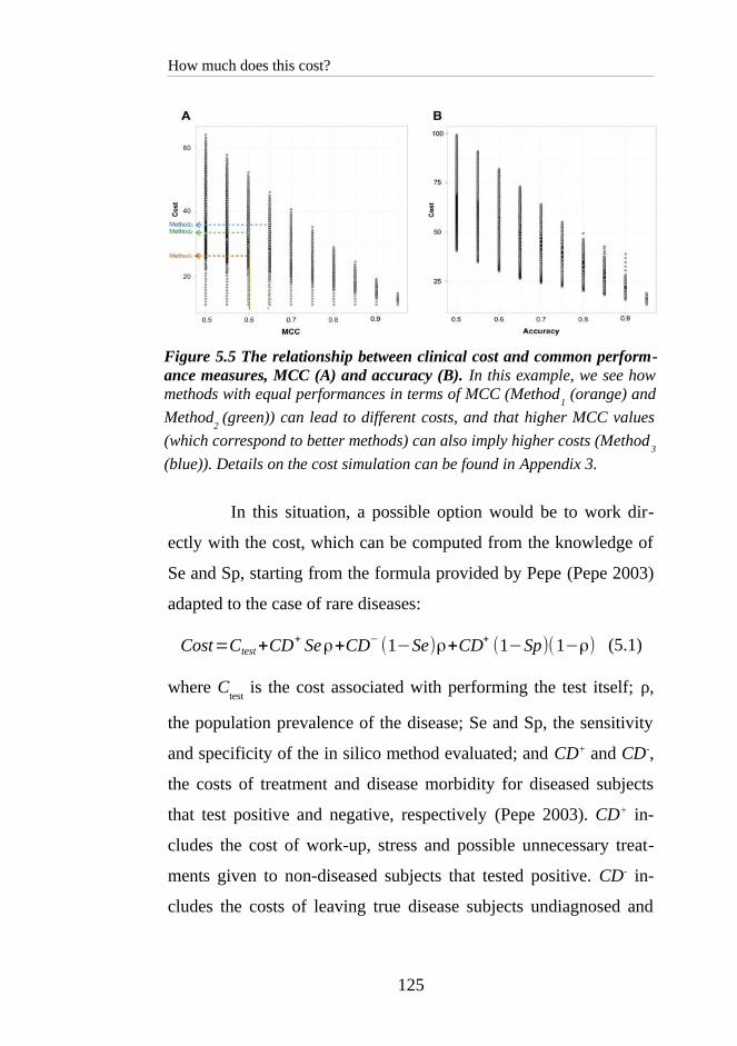
How much does this cost?
In this situation, a possible option would be to work dir-
ectly with the cost, which can be computed from the knowledge of
Se and Sp, starting from the formula provided by Pepe (Pepe 2003)
adapted to the case of rare diseases:
Cost=Ctest+CD+ Seρ+CD−(1−Se)ρ+CD+
(1−Sp)(1−ρ) (5.1)
where Ctest
is the cost associated with performing the test itself; ρ,
the population prevalence of the disease; Se and Sp, the sensitivity
and specificity of the in silico method evaluated; and CD+ and CD-,
the costs of treatment and disease morbidity for diseased subjects
that test positive and negative, respectively (Pepe 2003). CD+ in-
cludes the cost of work-up, stress and possible unnecessary treat-
ments given to non-diseased subjects that tested positive. CD- in-
cludes the costs of leaving true disease subjects undiagnosed and
125
Figure 5.5 The relationship between clinical cost and common perform-ance measures, MCC (A) and accuracy (B). In this example, we see howmethods with equal performances in terms of MCC (Method
1 (orange) and
Method2
(green)) can lead to different costs, and that higher MCC values
(which correspond to better methods) can also imply higher costs (Method3
(blue)). Details on the cost simulation can be found in Appendix 3.

A simplified version of healthcare cost to evaluate pathogenicity predictors
therefore, untreated. CD- tends to be larger than CD+ because undia-
gnosed disease will ultimately be harder to treat successfully.
However, two severe limitations impede the use of explicit
costs as a general parameter to assess predictors. Firstly, cost is a
quantity hard to assess, as it depends on all the stakeholders in the
healthcare process: patients, hospitals, insurers, countries, etc. And
secondly, cost may vary widely between diseases, expanding over a
big range of values, from few $ to $105-$106 (Pepe 2003).
5.2.2 VarCost: an alternative to absolute cost
To surpass the aforementioned limitations we decided to
explore a feasible alternative to cost. We wanted to find a monoton-
ic function of cost, f(cost), so that any ranking of predictors ob-
tained with cost was equivalent to that obtained with f(cost) and
vice-versa. We also wanted an f(cost) that was independent of any
scale variation of cost. Our starting point for this quest was the
standard cost/risk equation (5.1) provided by Pepe (Pepe 2003). Fi-
nally, since the focus of this work is to compare in silico predictors
from a diagnostic perspective, but not to assess the costs of introdu-
cing a specific treatment into the health system, we set the value of
ρ to 0.5. This starting point is further supported by the fact that the
frequency of a disease in a hospital environment does not reflect the
prevalence of the disease in the general population. With all these
points in mind, we rearranged (5.1) according to the following
steps:
Cost=Ctest+CD+ Seρ+CD−(1−Se)ρ+CD+
(1−Sp)ρ
Cost=Ctest+CD+ Seρ+CD− ρ−CD− Seρ+CD+ ρ−CD+ Spρ
126

How much does this cost?
Cost=Ctest+ρ(CD+ Se+CD−−CD− Se+CD+
−CD+ Sp)
Cost=Ctest+ρ(CD++CD−
)(CD+
CD++CD−
(Se−Sp)−CD−
CD++CD−
Se+1)
if we define:
α=ρ(CD++CD−
)
β+=
CD+
CD++CD−
β−=
CD−
CD++CD−
so that β−+β
+=1
therefore:
Cost=Ctest+α(β+(Se−Sp)−(β
−)Se+1)
Cost=Ctest+α(β+ (Se−Sp)−(1−β+ )Se+1)
Cost=Ctest+α+α(β+(2 Se−Sp)−Se)
Cost=C 'test+α ·VarCost (5.2)
where C ' test=C test+α
VarCost=β+(2 Se−Sp)−Se (5.3)
Looking at equation (5.2) we see that cost is a monotonical
function of VarCost; this is one of the conditions we imposed to our
new parameter. Also, VarCost does not depend on changes in cost
scale since is a relative value. Finally, VarCost depends on two
variables related to the performance of the predictor: Se and Sp. On
this basis, we propose VarCost as a new parameter for evaluating
127

A simplified version of healthcare cost to evaluate pathogenicity predictors
pathogenicity predictors, taking into account the value of clinical
costs.
VarCost has the virtue that any method selection based on its
use is completely equivalent to using the Cost formula because they
are monotonically related. A precise use of VarCost requires a
knowledge of the quantities CD+ and CD-, which are obviously hard
to estimate. However, because we work with their ratio, we can
obtain intuitive inequalities between treatment (CD+) and morbidity
(CD-) costs (e.g. relationships of the kind: the treatment costs are
roughly twice morbidity costs, etc.). These can help defining a
range of possible values, adapted for a particular disease or
treatment.
5.2.3 Profiling standard predictors with VarCost: discarding the concept of the absolutely best predictor
As we have mentioned before, pathogenicity predictors are
normally compared using parameters such as MCC, accuracy, etc.,
that were not conceived with clinical cost in mind. Once we ob-
tained the expression for VarCost, our next step was to apply it to a
set of representative tools and see what the resulting view was. In
particular, we wanted to see whether we could identify the "best"
pathogenicity predictor among all of them, an issue frequently ad-
dressed in benchmark studies (Thusberg and Vihinen 2009; Vihinen
2013; Martelotto et al. 2014; Schaafsma and Vihinen 2015).
For this comparison, we took advantage of the fact that
VarCost allows a characterization of the methods across the whole
cost range, in the form of a straight line. Indeed, if we look at equa-
128

How much does this cost?
tion (5.3), we see that it corresponds to the equation of a straight
line, where the independent variable is , and the slope and the in-
tercept are 2Se-Sp and -Se, respectively. From this starting point,
different situations may happen when we compare two methods:
• if their corresponding lines cross within range, we will
say that at the intersection point both methods will be
equally performing, that to the right of this point one method
will outperform the other, and that the opposite will happen
to the left of this point.
• if their corresponding lines do not cross within range, we
will say that the method with the line below is better, from
the point of view of cost, that the other.
• if their corresponding lines are equal, we will say that both
methods are comparable from the point of view of cost.
129

A simplified version of healthcare cost to evaluate pathogenicity predictors
In Figure 5.6A we display the VarCost lines for a set of
known predictors. A first important trend appears, which is the fol-
lowing: there is no best method preferable to the others, for the
whole cost range. There are only locally preferable methods. For
example, if we consider two of the most popular methods, SIFT and
PolyPhen-2 (Figure 5.6B) we see that for under 0.7 PolyPhen-2
can lead to smaller VarCost (and consequently to smaller total
costs), while for beta range 0.7 to 1, SIFT gives the optimum solu-
tion in terms of cost. We also identified some cases where one
130
Figure 5.6 Comparison of different in silico methods using VarCost. Inall the figures we represent VarCost as a function of for different meth-ods. (A) Behaviour of some of the most common methods. (B) SIFT (Simet al. 2012) vs. PolyPhen-2 (Adzhubei et al. 2010), (C) Comparisonbetween SNPs&GO (Calabrese et al. 2009), MutationTaster (Schwarz etal. 2010) and PredictSNP (Bendl et al. 2014), (D) Comparison betweentwo versions of PolyPhen-2: HumVar and HumDiv.

How much does this cost?
method is clearly preferable to others, that is, its VarCost line is be-
low the others' lines across the whole range. We can see this in
Figure 5.6C, where MutationTaster always has smaller VarCost val-
ues compared to PredictSNP. An interesting point appears when we
compare the two versions of PolyPhen-2 (Figure 5.6D): HumVar
and HumDiv. According to the authors, HumVar is preferable for
scoring causative variants of mendelian diseases, while HumDiv is
preferable for scoring variants potentially involved in complex
phenotypes (Adzhubei et al. 2016). However, when we compare
them at the cost level, we see that the HumDiv version may give
better results in from 0 to 0.6, regardless of whether the disease
considered is mendelian or not. In summary, when prediction meth-
ods are applied to the clinical diagnosis, these 'a priori' reasonings
based on conservation properties, etc., may not be the best choice.
As a note of caution, it has to be mentioned that these
curves have been obtained using the Se and Sp values provided by
the authors of the different methods in their articles (Adzhubei et al.
2010; Schwarz et al. 2010; Sim et al. 2012; Bendl et al. 2014).
Therefore, some level of variability is expected in the precise com-
parisons, however, we do not expect any change in the general
trends. This can be verified, and we are at present working in this
direction, by comparing different in silico methods on the same
dataset of interest (e.g. using all mutations available for a certain
disease).
5.2.4 VarCost vs. AUC/ROC
As we have seen AUC is a performance measure broadly
used in the clinical setting and for this reason we devote this final
131

A simplified version of healthcare cost to evaluate pathogenicity predictors
section to explore how it compares with VarCost. In particular, we
check how VarCost can help overcome a classical problem with
AUC. We have already mentioned that AUC can be misleading
when the curves of different methods cross: one method may have
the largest AUC, even if the other method has better performance
over a broader range of specificity values. For example, in Figure
5.7A, a protein specific predictor (PSP) for USH2A (data from
Chapter 4) has an AUC of 0.877, while PolyPhen-2 has an AUC
value of 0.923. However, at the default decision threshold for each
method, the PSP has a better MCC than PolyPhen-2 (0.51 and 0.47
for PSP and PolyPhen-2, respectively). That is, there is a contradic-
tion between AUC-based and MCC-based resulting choice of meth-
ods. VarCost offers an alternative to resolve this situation. By plot-
ting the VarCost lines for the two methods, we can analyse their re-
lationship and unambiguously decide the best method according to
the value (or range of values) of interest. In this case, for lower
values of , PolyPhen-2 would be advisable, while for values
above 0.3, PSP gives better results, regarding cost. In Figure 5.7B
we find another situation of crossing ROCs in MYH7. Now, the
solution, in terms of VarCost would be the opposite: PolyPhen-2
gives smaller values of VarCost at higher .
132

How much does this cost?
5.3 Conclusion
Identifying the best tool among a series of pathogenicity
predictors is still an open issue, one that is particularly relevant be-
cause of its clinical applications. Unfortunately, current perform-
ance measures (MCC, accuracy, AUC/ROC, etc.) do not take into
account one of the main factors in clinical applications: cost. Here,
we present VarCost, a novel performance measure that allows to
take into account cost in a very simple way and is specially suited
for the case of rare diseases. We show that VarCost is monotonically
related to the total cost, so that any decision based on VarCost is
equivalent to using total cost. In addition, this measure can be easily
computed from the Se and Sp of the method; it also offers a visual
133
Figure 5.7 Comparing ROC-based (upper plots) and VarCost (bottomplots) decisions for choosing the best prediction method for USH2A (A)and MYH7 (B). In blue, data for the protein specific predictor (PSP) and inred, for PolyPhen-2 (PPH). When using VarCost we easily see the regionsin which one method is preferable to the other in terms of clinical cost.

Conclusion
interpretation that helps the comparison between methods. Finally,
use of VarCost shows that the problem of choosing the best patho-
genicity predictor is an ill-posed problem from the point of view of
clinical cost, since at present there is no best predictor across the
whole cost range, there are only locally better predictors.
134

6 GENERAL
CONCLUSIONS

General Conclusions
136

General Conclusions
1. Exhaustive analysis of the current pathogenicity predictors
shows that they have reached a performance threshold
around 70-90% that is not enough for standalone clinical ap-
plications.
2. We have tested the use of protein-specific information with
the goal of breaking the prediction bottleneck in Fabry dis-
ease. Our results show that this is indeed possible and that a
protein-specific predictor can outperform state-of-the-art
general methods. This result holds for independent, valida-
tion datasets.
3. We have tested the hypothesis according to which protein-
specific methods always outperform general methods. We
find that this is not the case, and that the actual situation is
more complex: there is an important degree of complement-
arity between both approaches.
4. We find that the complementarity between PSP and GM is
independent of the methodology used to derive the PSP.
5. We observe that the complementarity between PSP and GM
can be used to obtain higher success rates in pathogenicity
prediction, respecting the limits set by the ACMG/AMP rule.
6. We have shown that current performance measures used to
evaluate pathogenicity predictors (MCC, accuracy, AUC/
ROC, etc.) are not adequate for assessing clinical cost.
137

General Conclusions
7. We have discovered a new parameter, VarCost, that can be
used to assess the performance of pathogenicity predictors in
terms of the clinical cost.
8. We have found, using VarCost, that the problem of choosing
the best pathogenicity predictor is an ill-posed problem from
the point of view of clinical cost. Indeed we find that there is
no best predictor across the whole cost range, there are only
locally better predictors.
138

7 APPENDICES


Appendices
APPENDIX 1
Table 7.1 List of the in silico methods used in Figure 2.1-2.2.
First column indicates the prediction method presented by the au-
thors. If there is no particular name given to the method or if the ar-
ticle simply reviews other prediction methods, not presenting any of
their own, we refer to the name of the first author in square brackets
(e.g. [Saunders]). Second column lists all the methods mentioned in
the paper. Methods used to benchmark appear grey-shaded and they
are only included in the 'global set' results. If authors provide more
than one version for their method, as in [Saunders], we only con-
sider the best one (bold line) for the 'best performance set'. Next
columns show accuracy, MCC and the reference, respectively.
Method Methods compared ACC MCC Reference
SIFT
SIFT (1) 0.683 0.350
Ng and
Henikoff
2001
Blosum62 (1) 0.542 -
SIFT (2) 0.780 0.510
Blosum62 (2) 0.699 -
SIFT (3) 0.634 0.290
Blosum62 (3) 0.470 -
SIFT (4) 0.699 0.400
PHD-SNP
PhD-SNP (1) 0.620 0.130
Capriotti et al.
2006
PhD-SNP (2) 0.700 0.340
PhD-SNP (3) 0.740 0.460
PolyPhen 0.720 0.440
SIFT 0.670 0.330
LRT
LRT 0.610 0.910Chun and Fay
2009PolyPhen 0.370 0.790
SIFT 0.530 0.880
141

Appendix 1
Method Methods compared ACC MCC Reference
FATHMM
FATHMM (1) 0.860 0.715
Shihab et al.
2012
FATHMM (2) 0.689 0.377
nsSNPAnalyzer 0.604 0.167
SNAP 0.739 0.474
MutPred 0.808 0.620
SIFT 0.648 0.302
PolyPhen1 (1) 0.692 0.393
PolyPhen1 (2) 0.696 0.397
Panther 0.765 0.528
PhD-SNP 0.718 0.433
SNPs&GO 0.817 0.652
PolyPhen-2 (1) 0.713 0.428
PolyPhen-2 (2) 0.681 0.393
FATHMM (3) 0.826 0.651
FATHMM (4) 0.731 0.427
MutPred 0.902 0.797
SIFT 0.758 0.492
PolyPhen1 0.724 0.463
Panther 0.700 0.362
PhD-SNP seq 0.709 0.398
PhD-SNP prof 0.785 0.558
SNPs&GO 0.833 0.653
PolyPhen-2 Div 0.708 0.463
PolyPhen-2 Var 0.716 0.479
SNAP
SNAP 0.790 0.582Bromberg and
Rost 2007SIFT 0.740 0.488
PolyPhen 0.749 0.503
PolyPhen PolyPhen 0.684 0.302Sunyaev et al.
2001
[Saunders][Saunders] (1) 0.780 0.540 Saunders and
Baker 2002[Saunders] (2) 0.710 0.360
SAAPredSAAPred - 0.692
Al-NumairPolyPhen-2 - 0.572
142

Appendices
Method Methods compared ACC MCC Reference
and Martin
2013
SIFT - 0.528
MutAss - 0.453
SIFTSIFT (1) 0.780 0.540 Sim et al.
2012SIFT (2) 0.850 0.660
SNPs&GO
SNPs&GO 0.820 0.630
Calabrese et
al. 2009
PolyPhen 0.710 0.390
SIFT 0.760 0.520
PANTHER 0.740 0.580
FFF FFF 0.830 0.590Herrgard et
al. 2003
FunSav
FunSav 0.799 0.598
Wang et al.
2012
SNAP 0.680 0.426
SIFT 0.734 0.475
PolyPhen-2 0.745 0.512
nsSNPAnalyzer 0.665 0.334
PANTHER 0.749 0.500
PhD-SNP 0.676 0.350
SNPanalyzer
SNPanalyzer (1) 0.682 0.274Bao et al.
2005SNPanalyzer (2) 0.708 0.315
SIFT 0.700 0.305
PON-P2
PON-P2 (1) 0.860 0.710
Niroula et al.
2015
PON-P2 (2) 0.770 0.530
Condel 0.750 0.490
PolyPhen-2 0.730 0.480
Provean 0.730 0.460
SIFT 0.740 0.480
SNAP 0.750 0.510
PON-P 0.850 0.690
MutationT-
aster
MutationTaster 0.860 0.710 Schwarz et al.
2010PolyPhen-2 (HumVar) 0.810 0.620
PolyPhen-2 (HumDiv) 0.800 0.610
SNAP 0.690 0.350
143

Appendix 1
Method Methods compared ACC MCC Reference
PANTHER 0.510 0.020
PMut 0.650 0.310
PMut PMut 0.835 0.670Ferrer-Costa
et al. 2004
I-Mutant2.0 I-Mutant2.0 0.800 0.510Capriotti et al.
2005
B-SIFT B-SIFT 0.700 -Lee et al.
2009
MutPred
MutPred (1) 0.628 -
Li et al. 2009
MutPred (2) 0.624 -
MutPred (3) 0.765 0.440
MutPred (4) 0.803 0.410
SIFT (1) 0.626 -
SIFT (2) 0.599 -
SIFT (3) 0.723 0.370
SIFT (4) 0.740 0.410
MutPred
SpliceMutPred Splice 0.788 0.540
Mort et al.
2014
SNPPer
SNPPer 0.800 -
Cai et al.
2004
[Ng 2001] 0.680 -
[Chasman & Adams] 0.800 -
[Krishnan & Westhead ] 0.840 -
[Chasman &
Adams]
[Chasman & Adams] (1) 0.671 0.332 Chasman and
Adams 2001[Chasman & Adams] (2) 0.779 0.523
MUpro MUpro 0.810 0.490Cheng et al.
2006
IPTREE-
STABIPTREE-STAB 0.814 -
Huang et al.
2007
[Huang][Huang] 0.800 - Huang et al.
2010SIFT 0.711 -
144

Appendices
Method Methods compared ACC MCC Reference
[Zhao] [Zhao] 0.828 -Zhao et al.
2014
SNPs3D SNPs3D 0.765 -Wang and
Moult 2001
CUPSAT CUPSAT 0.800 -Parthibam et
al. 2006
PPSC
PPSC (1) 0.790 0.480
Yang et al.
2013
PPSC (2) 0.850 0.650
FoldX 0.700 0.350
I-Mutant 2.0 0.840 0.610
MUpro 0.840 0.610
PROVEAN
PROVEAN 0.791 0.567
Choi et al.
2012
MutationAssessor 0.782 0.541
SIFT 0.770 0.519
PolyPhen-2 0.756 0.495
DDIG-in (FS)
DDIG-in (FS) 0.790 0.590Folkman et al.
2014SIFT indel 0.630 0.290
CADD indel 0.690 0.380
SIFT indel SIFT indel 0.840 -Hu and Ng
2012
PredictSNP
PredictSNP 0.747 0.492
Bendl et al.
2014
MAPP 0.711 0.423
nsSNPAnalyzer 0.629 0.219
PANTHER 0.658 0.296
PhD-SNP 0.751 0.494
PolyPhen-1 0.686 0.364
PolyPhen-2 0.691 0.407
SIFT 0.718 0.447
SNAP 0.680 0.346
PredictSNP 0.708 0.362
Condel 0.671 0.210
Meta-SNP 0.690 0.336
145

Appendix 1
Method Methods compared ACC MCC Reference
Condel
Condel 0.882 -
González-
Pérez and
López-Bigas
2011
SIFT 0.728 -
LogRe 0.690 -
PolyPhen-2 0.749 -
MAPP 0.764 -
MutAssessor 0.771 -
CAROL
CAROL 0.745 0.432Lopes et al.
2012PolyPhen-2 0.721 0.389
SIFT 0.744 0.210
PON-P
PON-P 0.690 0.390
Olastubosun
et al. 2012
PhD-SNP 0.640 0.280
SIFT 0.620 0.270
PolyPhen-2 0.660 0.270
SNAP 0.630 0.270
[Dorfman]
PANTHER 0.777 -Dorfman et
al. 2010SIFT 0.705 -
PolyPhen-2 0.568 -
PaPi
PaPi 0.862 0.724
Limongelli et
al. 2015
RF 0.826 0.652
PolyPhen-2 0.842 0.685
SIFT 0.805 0.611
EFIN
EFIN 0.837 -
Zeng et al.
2014
GERP 0.528 -
PhyloP 0.545 -
MutationTaster 0.795 -
SIFT 0.766 -
[Li] PlyloP 0.645 0.300 Li et al. 2014
GERP 0.635 0.281
SiPhy 0.665 0.342
SIFT 0.680 0.350
PolyPhen-2 HDIV 0.700 0.447
PolyPhen-2 Hvar 0.710 0.434
LRT 0.625 0.324
146

Appendices
Method Methods compared ACC MCC Reference
MutationTaster 0.600 0.333
MutationAssessor 0.690 0.362
FATHMM 0.520 0.127
RadialSVM score 0.690 0.474
LR score 0.635 0.393
MAPPMAPP 0.804 -
Stone and
Sidow 2005
SIFT 0.786 -
MutationAs-
sessorMutationAssessor 0.760 -
Reva et al.
2011
Meta-SNP
Meta-SNP 0.790 0.590
Capriotti et al.
2014
PANTHER 0.740 0.820
PhD-SNP 0.760 0.530
SIFT 0.700 0.410
SNAP 0.640 0.330
INPS
INPS 0.760 0.460
Fariselli et al.
2015
MuProSVM 0.690 0.070
Imutant3 0.670 0.070
AutomuteRF 0.740 0.000
isStable 0.260 0.000
Duet 0.790 0.360
mCSM 0.790 0.380
SDM 0.620 0.070
PopMusic2 0.690 0.120
NeEMO 0.640 0.090
Action
Action 0.781 -Katsonis and
Lichtarge
2014
PolyPhen-2 0.750 -
SIFT 0.745 -
MAPP 0.740 -
SeqProfCod SeqProfCod 0.820 0.590 Capriotti et al.
2008SIFT 0.710 0.380
PANTHER 0.740 0.430
SeqProfCod (Val) 0.740 0.480
147

Appendix 1
Method Methods compared ACC MCC Reference
SIFT (Val) 0.710 0.420
PANTHER (val) 0.770 0.520
SVM-3D
SVM-3D 0.850 0.700
Capriotti et al.
2011
SVM-3D 0.820 0.630
SVM-seq 0.820 0.640
SVM-seq 0.800 0.590
SIFT 0.770 0.530
PolyPhen-2 0.800 0.600
[Thusberg]
MutPred 0.810 0.630
Thusberg et
al. 2011
nsSNPAnalyzer 0.600 0.190
Panther 0.760 0.530
PhD-SNP 0.710 0.430
SNAP 0.720 0.470
SNPs&GO 0.820 0.650
SIFT 0.650 0.300
KGGseq KGGseq 0.775 - Li et al. 2012
[Needham] [Needham] 0.830 0.460Needham et
al. 2006
FuzzySnps FuzzySnps 0.285 0.460BArenboim et
al. 2008
[Karchin] [Karchin] 0.680 -Karchin et al.
2005
[Juritz] [Juritz] 0.680 0.360Juritz et al.
2012
[Li][Li] - 0.664
Li et al. 2013Condel - 0.616
148

Appendices
Method Methods compared ACC MCC Reference
sinBaD sinBaD 0.820 -Lehman and
Cheng 2013
[Krishnan] [Krishnan] 0.720 0.420
Krishnan and
Westhead
2003
[Cai] [Cai] 0.680 0.410Cai et al.
2004
[Huang]
[Huang] (1) 0.83 0.66
Huang et al.
2010
[Huang] (2) 0.800 -
SIFT (1) 0.711 -
SIFT (2) 0.71 -
[Li]
[Li] 0.81 0.59
Li et al. 2011
[Li] - 37 0.81 0.6
Bongo 0.47 -
SIFT 0.76 0.51
PolyPhen-2 0.76 0.51
Table 7.1
149


Appendices
APPENDIX 2
Table 7.2 List of the in silico methods used in Chapter 4. Col-
umns 1-2 indicate the gene name and Uniprot ID, respectively. Col-
umn 3 corresponds to the number of pathological variants described
in Humsavar as 'Disease'. Column 4 is the number of neutral vari-
ants found in the homology model used in this work (see The vari-
ant datasets, page 90) and fifth column is the number of neutral
variants present in Humsavar, described as 'Polymorphism'. Final
column correspond to the protein sequence length in amino acids.
Gene Name Uniprot ID #Muts P#Muts N
(homol)
#Muts N
(freq)seqlenght
MEN1 O00255 96 193 2 615
NPC1 O15118 151 205 15 1278
RS1 O15537 64 63 2 224
SLC26A4 O43511 60 68 9 780
OPA1 O60313 52 346 6 960
NPHS1 O60500 61 52 6 1241
LRP5 O75197 53 505 9 1615
USH2A O75445 65 515 45 5202
BEST1 O76090 103 52 7 585
ABCC6 O95255 81 98 25 1503
PAH P00439 206 55 1 452
F8C P00451 472 247 7 2351
OTC P00480 111 105 6 354
HPRT1 P00492 62 64 0 218
ASS1 P00966 61 142 1 412
COL1A1 P02452 129 482 16 1464
COL2A1 P02458 57 613 7 1487
COL3A1 P02461 101 93 9 1466
LMNA P02545 115 217 2 664
151

Appendix 2
Gene Name Uniprot ID #Muts P#Muts N
(homol)
#Muts N
(freq)seqlenght
F11 P03951 53 76 5 625
ASL P04424 57 109 0 464
CYBB P04839 64 75 3 570
GLA P06280 157 56 0 429
PROS1 P07225 90 58 8 676
RET P07949 106 87 9 1114
GJB1 P08034 186 78 0 283
RHO P08100 69 91 2 348
COL1A2 P08123 78 63 18 1366
HMBS P08397 84 52 0 361
CYP21A2 P08686 58 71 5 494
PKHD1 P08F94 99 388 39 4074
GAA P10253 130 91 22 952
AR P10275 160 65 3 919
FGFR1 P11362 69 316 6 822
MYH7 P12883 187 541 9 1935
CFTR P13569 146 215 30 1480
ARSA P15289 97 61 8 507
SMPD1 P17405 80 50 5 629
CAPN3 P20807 53 103 5 821
NF1 P21359 84 1271 14 2839
FGFR2 P21802 55 300 4 821
RYR1 P21817 146 738 24 5038
MUT P22033 84 204 5 750
IDS P22304 126 78 0 550
TGM1 P22735 64 77 6 817
MPZ P25189 74 58 1 248
COL4A5 P29400 145 156 7 1685
CPS1 P31327 134 412 6 1500
ABCD1 P33897 136 60 1 745
IDUA P35475 51 72 9 653
SCN1A P35498 186 587 10 2009
152

Appendices
Gene Name Uniprot ID #Muts P#Muts N
(homol)
#Muts N
(freq)seqlenght
FBN1 P35555 249 1162 20 2871
ATP7B P35670 194 130 23 1465
MLH1 P40692 67 65 17 756
CASR P41180 62 186 6 1078
MSH2 P43246 61 272 12 934
PSEN1 P49768 74 104 2 467
TSC2 P49815 52 219 30 1807
PPOX P50336 56 67 1 477
SGSH P51688 56 50 7 502
POLG P54098 62 85 9 1239
SLC12A3 P55017 75 106 5 1021
PLP1 P60201 69 53 0 277
ACTA1 P68133 78 149 0 1685
ABCA4 P78363 199 324 22 2273
JAG1 P78504 52 614 4 1218
CRB1 P82279 70 186 9 1406
COL7A1 Q02388 75 296 5 2944
PTPN11 Q06124 50 230 0 597
BTK Q06187 110 222 2 659
ABCC8 Q09428 70 625 9 1581
KCNH2 Q12809 104 341 10 1159
MYO7A Q13402 50 1186 10 2215
MTM1 Q13496 57 220 0 603
SCN5A Q14524 154 333 14 2016
MYBPC3 Q14896 64 144 13 1274
CNGA3 Q16281 59 58 7 694
GCDH Q92947 58 72 2 438
MYOC Q99972 57 65 26 504
CDH23 Q9H251 56 509 61 3354
SPAST Q9UBP0 62 138 3 616
NOTCH3 Q9UM47 110 368 6 2321
Table 7.2
153


Appendices
APPENDIX 3
To generate the simulations presented in Figure 5.5A we
followed a simple protocol, based on generating random quartets
(TP, TN, FP and FN) that obeyed a specific restraint (they had to
correspond to a given MCC or accuracy values) and were used to
compute cost using the cost equation (see equation 5.1, page 125)
(Pepe 2003). The generation of these quartets followed a simple
scheme; I explain it for MCC, although for accuracy it was com-
pletely analogous (see below). For TN, FP and FN, we systematic-
ally varied them between 0 and 1000 in intervals of 10 (e.g. TN=0,
10, 20, ...) and we did the same for the MCC between 0.5 and 1 in
intervals of 0.05. Below we give a simple scheme of this procedure.
Then, for each resulting set of values, we replaced their values in
equation (7.2), to compute TP. Finally, we used the resulting TP
value, together with TN, FP and FN to calculate Se and Sp that
would be used in the cost expression. Schematically:
For MCC between 0.5 to 1, step 0.05:
For TN between 0 to 1000, step 10:
FP = 1000 – TN
For FN between 0 to 1000, step 10:
Solve TP, given MCC, TN, FP and FN
Calculate Se and Sp, given TP, TN, FP, FN
Calculate Cost, given Se, Sp, rho, CD+, CD-
155

Appendix 3
To obtain an expression for TP as a function of TN, FP, FN
and MCC, our starting point was the formal definition of the MCC:
MCC=TP⋅TN −FP⋅FN
√(TP+FP)(TP+FN )(TN +FP)(TN +FN )(7.1)
MCC2=
TP⋅TN−FP⋅FN 2
(TP+FP)(TP+FN )(TN +FP)(TN+FN )
MCC2(TP+FP)(TP+FN )(TN+ FP)(TN +FN )=(TP⋅TN−FP⋅FN )
2
MCC2(TN +FP)(TN +FN )[TP2
+(FP+FN )TP+FP·FN ]=
TP2· TN 2−2 ·TP·TN·FP·FN +FN 2· FP2
After substracting common factor and rearranging:
TP2[TN 2
−MCC2(TN +FP)(TN +FN )]−
−TP [2 ·TN·FP·FN + MCC2(TN +FP)(TN+FN)(FN +FP)]+
+FP2· FN 2−MCC2
(TN +FP)(TN +FN )(FP·FN )=0
This equation is quadratic in TP:
TP2 · a−TP·b+c=0
We solve it using the standard formula:
x=−b±√b2
−4 ac2 a
Applying this formula we can express TP as:
TP=A±B√C
D(7.2)
where A, B, C and D correspond to:
A=2TN·FP·FN +MCC2(TN +FP)(TN +FN )(FN +FP)
156

Appendices
B=MCC (TN +FP)(TN +FN )(FN−FP)
C=MCC2+4 FP·FN·TN (FN+FP)+FN·FP+TN 2
(TN +FP )(TN +FN )(FN−FP)2
D=2(TN 2−MCC2
(TN +FP)(TN +FN ))
Figure 5.5B was obtained equivalently but starting from
the accuracy equation (7.3). First, I systematically varied TN, FP
and FN between 0 and 1000 in intervals of 10, and accuracy
between 0.5 and 1 in intervals of 0.05. Then, for each quartet I used
the accuracy equation (7.3) to obtain the TP value (7.4):
Accuracy=Acc=TP+TN
TP+FN +TN+FP (7.3)
Acc (TP+FN +TN+FP)=TP+TN
Acc·TP−TP=TN−Acc·TN−Acc·FP−Acc·FN
TP( Acc−1)=TN (1−Acc)−(FP+FN ) Acc
TP=TN−Acc (TN+FP+FN )
Acc−1 (7.4)
Finally, I used the resulting TP value, together with TN, FP
and FN to calculate Se and Sp that would be used in the cost equa-
tion, described before.
157


8 BIBLIOGRAPHY


Bibliography
Adams NM, Hand DJ. 1999. Comparing classifiers when the misalloca-tion costs are uncertain. Pattern Recognit. 32: 1139–1147.
Adebali O, Reznik AO, Ory DS, Zhulin IB. 2016. Establishing the preciseevolutionary history of a gene improves prediction of disease-causingmissense mutations. Genet. Med.
Adzhubei I, Schmidt S, Peshkin L, Ramensky V, Gerasimova A, Bork P,Kondrashov A, Sunyaev S. 2016.
Adzhubei I, Schmidt S, Peshkin L, Ramensky VE, Bork P, KondrashovAS, Sunyaev SR. 2010. A method and server for predicting damaging mis-sense mutations. Nat. Methods 7: 248–249.
Al-Numair NS, Martin ACR. 2013. The SAAP database and pipeline:tools to analyze the impact and predict the pathogenicity of mutations.BMC Genomics.
Ali H, Olatubosun A, Vihinen M. 2012. Classification of mismatch repairgene missense variants with PON-MMR. Hum. Mutat. 33: 642–50.
Altschul SF, Gertz EM, Agarwala R, Schäffer A a, Yu Y-K. 2009. PSI-BLAST pseudocounts and the minimum description length principle.Nucleic Acids Res. 37: 815–24.
Amberger J, Bocchini CA, Scott AF, Hamosh A. 2009. McKusick’s On-line Mendelian Inheritance in Man (OMIM). Nucleic Acids Res. 37:D793–6.
Angarica VE, Orozco M, Sancho J. 2015. Exploring the complete muta-tional space of the LDL receptor LA5 domain using molecular dynamics:Linking snps with disease phenotypes in familial hypercholesterolemia.Hum. Mol. Genet. 25: 1233–1246.
Arias TD, Jorge LF, Barrantes R. 1991. Uses and misuses of definitions ofgenetic polymorphism. A perspective from population pharmacogenetics[letter]. Br. J. Clin. Pharmacol. 31: 117–120.
Aschauer L, Muller PAJ. 2016. Novel targets and interaction partners ofmutant p53 Gain-Of-Function. Biochem. Soc. Trans. 44: 460–466.
Ashburner M, Ball CA, Blake JA, Botstein D, Butler H, Cherry JM, DavisAP, Dolinski K, Dwight SS, Eppig JT, Harris MA, Hill DP, et al. 2000.Gene ontology: tool for the unification of biology. The Gene OntologyConsortium. Nat. Genet. 25: 25–29.
161

Bibliography
Ashenberg O, Gong LI, Bloom JD. 2013. Mutational effects on stabilityare largely conserved during protein evolution. Proc. Natl. Acad. Sci. U.S. A. 110: 21071–21076.
Baase WA, Liu L, Tronrud DE, Matthews BW. 2010. Lessons from thelysozyme of phage T4. Protein Sci. 19: 631–641.
Bagci Z, Jernigan RL, Bahar I. 2002. Residue coordination in proteinsconforms to the closest packing of spheres. Polymer (Guildf). 43: 451–459.
Bairoch A, Apweiler R, Wu CH, Barker WC, Boeckmann B, Ferro S,Gasteiger E, Huang H, Lopez R, Magrane M, Martin MJ, Natale DA, etal. 2005. The Universal Protein Resource (UniProt). Nucleic Acids Res.33: D154–9.
Baldi P, Brunak S. 2001. Bioinformatics: The Machine Learning Ap-proach. Cambridge, Massachusetts: The MIT Press.
Baldi P, Brunak S, Chauvin Y, Andersen CAF, Nielsen H. 2000. Assessingthe accuracy of prediction algorithms for classification: an overview.Bioinformatics 16: 412–424.
Bamshad MJ, Ng SB, Bigham AW, Tabor HK, Emond MJ, Nickerson D a,Shendure J. 2011. Exome sequencing as a tool for Mendelian disease genediscovery. Nat. Rev. Genet. 12: 745–55.
Bao L, Cui Y. 2005. Prediction of the phenotypic effects of non-synonym-ous single nucleotide polymorphisms using structural and evolutionary in-formation. Bioinformatics 21: 2185–90.
Barenboim M, Masso M, Vaisman II, Jamison DC. 2008. Statistical geo-metry based prediction of nonsynonymous SNP functional effects usingrandom forest and neuro-fuzzy classifiers. Proteins 71: 1930–1939.
Baresic A, Hopcroft LEM, Rogers HH, Hurst JM, Martin ACR. 2010.Compensated pathogenic deviations: analysis of structural effects. J. Mol.Biol. 396: 19–30.
Bendl J, Stourac J, Salanda O, Pavelka A, Wieben ED, Zendulka J,Brezovsky J, Damborsky J. 2014. PredictSNP: robust and accurate con-sensus classifier for prediction of disease-related mutations. PLoS Com-put. Biol. 10: e1003440.
162

Bibliography
Berg JS, Adams M, Nassar N, Bizon C, Lee K, Schmitt CP, WilhelmsenKC, Evans JP. 2013. An informatics approach to analyzing the incidenta-lome. Genet. Med. 15: 36–44.
Bishop CM. 1995. Neural Networks for Pattern Recognition. Oxford: Ox-ford University Press.
Bishop CM. 2006. Pattern Recognition and Machine Learning. New York:Springer.
Bonastre J, Marguet S, Lueza B, Michiels S, Delaloge S, Saghatchian M.2014. Cost effectiveness of molecular profiling for adjuvant decision mak-ing in patients with node-negative breast cancer. J. Clin. Oncol. 32: 3513–3519.
Bondi A. 1964. van der Waals Volumes and Radii. J. Phys. Chem. 68:441–451.
Boyko EJ. 1994. Ruling out or ruling in disease with the most sensitive orspecific diagnostic test: Short cut or wrong turn? Med. Decis. Mak. 14:174–179.
Breen MS, Kemena C, Vlasov PK, Notredame C, Kondrashov FA. 2012.Epistasis as the primary factor in molecular evolution. Nature 490: 535–538.
Bromberg Y, Rost B. 2007. SNAP: predict effect of non-synonymouspolymorphisms on function. Nucleic Acids Res. 35: 3823–3835.
Bromberg Y, Rost B. 2009. Correlating protein function and stabilitythrough the analysis of single amino acid substitutions. BMC Bioinform-atics 10.
Bromberg Y, Yachdav G, Rost B. 2008. SNAP predicts effect of mutationson protein function. Bioinformatics 24: 2397–2398.
Cai Z, Tsung EF, Marinescu VD, Ramoni MF, Riva A, Kohane IS. 2004.Bayesian approach to discovering pathogenic SNPs in conserved proteindomains. Hum. Mutat. 24: 178–84.
Calabrese R, Capriotti E, Fariselli P, Martelli PL, Casadio R. 2009. Func-tional annotations improve the predictive score of human disease-relatedmutations in proteins. Hum. Mutat. 30: 1237–1244.
163

Bibliography
Capriotti E, Altman R. 2011. Improving the prediction of disease-relatedvariants using protein three-dimensional structure. BMC Bioinformatics12: S3.
Capriotti E, Arbiza L, Casadio R, Dopazo J, Dopazo H, Marti-RenomMA. 2008. Use of estimated evolutionary strength at the codon level im-proves the prediction of disease-related protein mutations in humans.Hum. Mutat. 29: 198–204.
Capriotti E, Calabrese R, Casadio R. 2006. Predicting the insurgence ofhuman genetic diseases associated to single point protein mutations withsupport vector machines and evolutionary information. Bioinformatics 22:2729–34.
Capriotti E, Fariselli P, Casadio R. 2005. I-Mutant2.0: predicting stabilitychanges upon mutation from the protein sequence or structure. NucleicAcids Res. 33: W306–10.
Cardoso RM, Thayer MM, DiDonato M, Lo TP, Bruns CK, Getzoff ED,Tainer JA. 2002. Insights into Lou Gehrig’s disease from the structure andinstability of the A4V mutant of human Cu,Zn superoxide dismutase. J.Mol. Biol. 324: 247–256.
Care MA, Needham CJ, Bulpitt AJ, Westhead DR. 2007. Deleterious SNPprediction: be mindful of your training data! Bioinformatics 23: 664–672.
Chasman D, Adams RM. 2001. Predicting the functional consequences ofnon-synonymous single nucleotide polymorphisms: structure-based as-sessment of amino acid variation. J. Mol. Biol. 307: 683–706.
Chawla N V, Bowyer KW, Hall LO, Kegelmeyer WP. 2002. SMOTE:Synthetic Minority Over-sampling TEchnique. J. Artif. Intell. Res. 16:341–78.
Choi Y, Sims GE, Murphy S, Miller JR, Chan AP. 2012. Predicting thefunctional effect of amino Acid substitutions and indels. PLoS One 7:e46688.
Chun S, Fay JC. 2009. Identification of deleterious mutations within threehuman genomes. Genome Res. 19: 1553–61.
Cline MS, Karchin R. 2011. Using bioinformatics to predict the functionalimpact of SNVs. Bioinformatics 27: 441–448.
164

Bibliography
Cole C, Barber JD, Barton GJ. 2008. The Jpred 3 secondary structure pre-diction server. Nucleic Acids Res. 36: W197–201.
Cooper DN, Krawczak M, Polychronakos C, Tyler-Smith C, Kehrer-Sawatzki H. 2013. Where genotype is not predictive of phenotype: to-wards an understanding of the molecular basis of reduced penetrance inhuman inherited disease. Hum. Genet.
Corbett-Detig RB, Zhou J, Clark AG, Hartl DL, Ayroles JF. 2013. Geneticincompatibilities are widespread within species. Nature 504: 135–137.
Creighton T, Goldenberg DP. 1992. Mutational Analysis of Protein Fold-ing and Stability. In: Creighton T, editors. Protein Folding, New York: W.H. Freeman and Company, p 353–403.
Crockett DK, Lyon E, Williams MS, Narus SP, Facelli JC, Mitchell JA.2012. Utility of gene-specific algorithms for predicting pathogenicity ofuncertain gene variants. J. Am. Med. Informatics Assoc. 19: 207–211.
Cui Q, Karplus M. 2008. Allostery and cooperativity revisited. ProteinSci. 17: 1295–1307.
Desnick RJ, Ioannou YA, Eng CM, Scriver CR, Beaudet AL, Sly W, ValleD. 2005. a-galactosidase A deficiency: Fabry disease. The Metabolic andMolecular bases of inherited disease, p 3733–74.
DiDonato M, Craig L, Huff ME, Thayer MM, Cardoso RM, KassmannCJ, Lo TP, Bruns CK, Powers ET, Kelly JW, Getzoff ED, Tainer JA. 2003.ALS mutants of human superoxide dismutase form fibrous aggregates viaframework destabilization. J. Mol. Biol. 332: 601–615.
Dill KA. 1990. Dominant forces in protein folding. Biochemistry 29:7133–7155.
Do CB. The Multivariate Gaussian Distribution. 2008.
Duda RO, Hart PE, Stork DG. 2001. Pattern Classification. New York:John Wiley & Sons, Inc.
Durbin R, Eddy SR, Krogh A, Mitchinson G. 1998. Biological SequenceAnalysis: Probabilistic Models of Proteins and Nucleic Acids. Cambridge:Cambridge University Press.
Edgar RC. 2004. MUSCLE: multiple sequence alignment with high accur-acy and high throughput. Nucleic Acids Res. 32: 1792–1797.
165

Bibliography
Eitzman DT, Bodary PF, Shen Y, Khairallah CG, Wild SR, Abe A, Shaf-fer-Hartman J, Shayman JA. 2003. Fabry Disease in Mice Is AssociatedWith Age-Dependent Susceptibility to Vascular Thrombosis. J. Am. Soc.Nephrol. 14: 298–302.
Elias I. 2006. Settling the intractability of multiple alignment. J. ComputBiol 13: 1323–1339.
Eng CM, Banikazemi M, Gordon RE, Goldman M, Phelps R, Kim L,Gass A, Winston J, Dikman S, Fallon JT, Brodie S, Stacy CB, et al. 2001.A Phase 1/2 Clinical Trial of Enzyme Replacement in Fabry Disease:Pharmacokinetic, Substrate Clearance, and Safety Studies. Am. J. Hum.Genet. 68: 711–722.
Fariselli P, Martelli PL, Savojardo C, Casadio R. 2015. INPS: Predictingthe Impact of Non-Synonymous Variations on Protein Stability from Se-quence. Bioinformatics 1–6.
Fauchère J, Pliska V. 1983. Hydrophobic parameters of amino acid side-chains from the partitioning of N-acetyl-amino-acid amides. Eur. J. Med.Chem-Chim Ther 18: 369–375.
Fechter K, Porollo A. 2014. MutaCYP: Classification of missense muta-tions in human cytochromes P450. BMC Med. Genomics 7: 47.
Ferrer-Costa C, Gelpí JL, Zamakola L, Parraga I, de la Cruz X, Orozco M.2005a. PMUT: a web-based tool for the annotation of pathological muta-tions on proteins. Bioinformatics 21: 3176–3178.
Ferrer-Costa C, Orozco M, de la Cruz X. 2002. Characterization of dis-ease-associated single amino acid polymorphisms in terms of sequenceand structure properties. J. Mol. Biol. 315: 771–786.
Ferrer-Costa C, Orozco M, de la Cruz X. 2004. Sequence-based predictionof pathological mutations. Proteins 57: 811–9.
Ferrer-Costa C, Orozco M, de la Cruz X. 2005b. Use of bioinformaticstools for the annotation of disease-associated mutations in animal models.Proteins 61: 878–87.
Ferrer-Costa C, Orozco M, de la Cruz X. 2007. Characterization of com-pensated mutations in terms of structural and physico-chemical properties.J. Mol. Biol. 365: 249–256.
166

Bibliography
Fersht A. 1998. Structure and Mechanism in Protein Structure. New York:W. H. Freeman and Company.
Flanagan SE, Patch A-M, Ellard S. 2010. Using SIFT and PolyPhen topredict loss-of-function and gain-of-function mutations. Genet. Test. Mol.Biomarkers 14: 533–7.
Fokkema IF, Taschner PE, Schaafsma GC, Celli J, Laros JF, Dunnen JTden. 2011. LOVD v.2.0: the next generation in gene variant databases.Hum. Mutat. 32: 557–563.
Garman SC, Garboczi DN. 2002. Structural basis of Fabry disease. Mol.Genet. Metab. 77: 3–11.
Garman SC, Garboczi DN. 2004. The molecular defect leading to Fabrydisease: structure of human alpha-galactosidase. J. Mol. Biol. 337: 319–35.
Godoy-Ruiz R, Perez-Jimenez R, Ibarra-Molero B, Sanchez-Ruiz JM.2005. A stability pattern of protein hydrophobic mutations that reflectsevolutionary structural optimization. Biophys. J. 89: 3320–3331.
Gonzaga-Jauregui C, Lupski JR, Gibbs R. 2012. Human genome sequen-cing in health and disease. Annu Rev Med 63: 35–61.
González-Pérez A, López-Bigas N. 2011. Improving the assessment of theoutcome of nonsynonymous SNVs with a consensus deleteriousnessscore, Condel. Am. J. Hum. Genet. 88: 440–9.
Goodstadt L, Ponting CP. 2001. Sequence variation and disease in thewake of the draft human genome. Hum. Mol. Genet. 10: 2209–2214.
Grimm DG, Azencott C, Aicheler F, Gieraths U, MacArthur DG, SamochaKE, Cooper DN, Stenson PD, Daly M, Smoller JW, Duncan LE,Borgwardt KM, et al. 2015. The Evaluation of Tools Used to Predict theImpact of Missense Variants Is Hindered by Two Types of Circularity.Hum. Mutat. 1–37.
Hall M, Frank E, Holmes G, Pfahringer B, Reutemann P, Witten IH. 2009.The WEKA Data Mining Software: An Update. SIGKDD Explor. 11: 10–18.
Hamasaki-Katagiri N, Salari R, Wu A, Qi Y, Schiller T, Filiberto AC,Schisterman EF, Komar AA, Przytycka TM, Kimchi-Sarfaty C. 2013. A
167

Bibliography
Gene-Specific Method for Predicting Hemophilia-Causing Point Muta-tions. J. Mol. Biol. 425(21): 4023–4033.
Hand DJ. 2009. Measuring classifier performance: a coherent alternativeto the area under the ROC curve. Mach. Learn. 77: 103–123.
Hand DJ. 2010. Evaluating diagnostic tests: the area under the ROC curveand the balance of errors. 1–18.
Hand DJ. 2012. Assessing the Performance of Classification Methods. Int.Stat. Rev. 80: 400–414.
Hand DJ, Anagnostopoulos C. 2013. When is the area under de receiveroperating characteristic curve an appropriate measure of classifier per-formance? Pattern Recognit. Lett. 34: 492–495.
Hastie T, Tibshirani RJ, Friedman J. 2009. The Elements of StatisticalLearning. New York: Springer.
Henikoff S, Henikoff JG. 1992. Amino acid substitution matrices fromprotein blocks. Proc. Natl. Acad. Sci. 89: 10915–10919.
Henikoff S, Henikoff JG. 1994. Position-based sequence weights. J. Mol.Biol. 243: 574–578.
Hicks S, Wheeler DA, Plon SE, Kimmel M. 2011. Prediction of missensemutation functionality depends on both the algorithm and sequence align-ment employed. Hum. Mutat. 32: 661–668.
Hoffmann B. 2009. Fabry disease: recent advances in pathology, diagnos-is, treatment and monitoring. Orphanet J. Rare Dis. 4: 21.
Huang T, Wang P, Ye Z-QQ, Xu H, He Z, Feng K-YY, Hu L, Cui W, WangK, Dong X, Xie L, Kong X, et al. 2010. Prediction of Deleterious Non-Synonymous SNPs Based on Protein Interaction Network and HybridProperties. PLoS One 5: e11900.
Hubbard SJ, Thornton JM. 1993. “NACCESS”, Computer Program. Dep.Biochem. Mol. Biol. Univ. Coll. London.
Iseki E, Matsumura T, Marui W, Hino H, Odawara T, Sugiyama N, SuzukiK, Sawada H, Arai T, Kosaka K. 2001. Familial frontotemporal dementiaand parkinsonism with a novel N296H mutation in exon 10 of the taugene and a widespread tau accumulation in the glial cells. Acta Neuro-pathol 102: 285–292.
168

Bibliography
Izarzugaza JMG, Pozo A del, Vazquez M, Valencia A. 2012. Prioritizationof pathogenic mutations in the protein kinase superfamily. BMC Genom-ics 13 Suppl 4: S3.
Johansen MB, Izarzugaza JMG, Brunak S, Petersen TN, Gupta R. 2013.Prediction of Disease Causing Non-Synonymous SNPs by the ArtificialNeural Network Predictor NetDiseaseSNP. PLoS One 8: e68370.
Jordan DM, Kiezun A, Baxter SM, Agarwala V, Green RC, Murray MF,Pugh T, Lebo MS, Rehm HL, Funke BH, Sunyaev SR. 2011. Develop-ment and validation of a computational method for assessment of mis-sense variants in hypertrophic cardiomyopathy. Am. J. Hum. Genet. 88:183–192.
Juritz E, Fornasari MS, Martelli PL, Fariselli P, Casadio R, Parisi G. 2012.On the effect of protein conformation diversity in discriminating amongneutral and disease related single amino acid substitutions. BMC Genom-ics 13 Suppl 4: S5.
Karchin R, Diekhans M, Kelly L, Thomas DJ, Pieper U, Eswar N,Haussler D, Sali A. 2005a. LS-SNP: large-scale annotation of coding non-synonymous SNPs based on multiple information sources. Bioinformatics21: 2814–2820.
Karchin R, Kelly L, Sali A. 2005b. Improving functional annotation ofnon-synonomous SNPs with information theory. Pac Symp Biocomput397–408.
Karchin R, Monteiro AN, Tavtigian S V, Carvalho MA, Sali A. 2007.Functional impact of missense variants in BRCA1 predicted by supervisedlearning. PLoS Comput. Biol. 3: e26.
Katsonis P, Koire A, Wilson SSJ, Hsu TKT, Lua RC, Wilkins AD,Lichtarge O. 2014. Single nucleotide variations: Biological impact andtheoretical interpretation. Protein Sci. 23: 1650–1666.
Kent WJ, Sugnet CW, Furey TS, Roskin KM, Pringle TH, Zahler AM,Haussler D. 2002. The human genome browser at UCSC. Genome Res.12: 996–1006.
Khan S, Vihinen M. 2010. Performance of protein stability predictors.Hum. Mutat. 31: 675–684.
169

Bibliography
Khurana E, Fu Y, Chen J, Gerstein M. 2013. Interpretation of genomicvariants using a unified biological network approach. PLoS Comput. Biol.9: e1002886.
Kiezun A, Garimella K, Do R, Stitziel NO, Neale BM, McLaren PJ, GuptaN, Sklar P, Sullivan PF, Moran JL, Hultman CM, Lichtenstein P, et al.2012. Exome sequencing and the genetic basis of complex traits. Nat.Genet. 44: 623–30.
Kircher M, Witten DM, Jain P, O’Roak BJ, Cooper GM, Shendure J.2014. A general framework for estimating the relative pathogenicity of hu-man genetic variants. Nat. Genet. 46: 310–5.
Knight JC. 2009. Human Genetic Diversity: Functional Consequences forHealth and Disease. Oxford: Oxford University Press.
Kohane IS, Hsing M, Kong SW. 2012. Taxonomizing, sizing, and over-coming the incidentalome. Genet. Med. 14: 399–404.
Kondrashov AS, Sunyaev SR, Kondrashov FA. 2002. Dobzhansky-Mullerincompatibilities in protein evolution. Proc. Natl. Acad. Sci. 99: 14878–14883.
Kotera M, Hirakawa M, Tokimatsu T, Goto S, Kanehisa M. 2012. TheKEGG databases and tools facilitating omics analysis: latest developmentsinvolving human diseases and pharmaceuticals. Methods Mol. Biol. 802:19–39.
Krishnan VG, Westhead DR. 2003. A comparative study of machine-learning methods to predict the effects of single nucleotide polymorph-isms on protein function. Bioinformatics 19: 2199–2209.
Ku C-SS, Cooper DN, Polychronakos C, Naidoo N, Wu M, Soong R.2012. Exome sequencing: dual role as a discovery and diagnostic tool.Ann Neurol 71: 5–14.
Kumar P, Henikoff S, Ng PC. 2009. Predicting the effects of coding non-synonymous variants on protein function using the SIFT algorithm. Nat.Protoc. 4: 1073–81.
Kumar S, Sanderford M, Gray VE, Ye J, Liu L. 2012. Evolutionary dia-gnosis method for variants in personal exomes. Nat. Methods 9: 855–856.
Lander ES, Linton LM, Birren B, Nusbaum C, Zody MC, Baldwin J,Devon K, Dewar K, Doyle M, FitzHugh W, Funke R, Gage D, et al. 2001.
170

Bibliography
Initial sequencing and analysis of the human genome. Nature 409: 860–921.
Lee W, Zhang Y, Mukhyala K, Lazarus RA, Zhang Z. 2009. Bi-Direction-al SIFT Predicts a Subset of Activating Mutations. PLoS One 4: e8311.
Lehmann K V, Chen T. 2012. Exploring functional variant discovery innon-coding regions with SInBaD. Nucleic Acids Res. 41: e7.
Leong IUS, Stuckey A, Lai D, Skinner JR, Love DR. 2015. Assessment ofthe predictive accuracy of five in silico prediction tools, alone or in com-bination, and two metaservers to classify long QT syndrome gene muta-tions. BMC Med. Genet. 16: 34.
Li B, Krishnan VG, Mort M, Xin F, Kamati KK, Cooper DN, MooneySD, Radivojac P. 2009. MutPred: Automated inference of molecularmechanisms of disease from amino acid substitutions. Bioinformatics 25:2744–2750.
Li MX, Gui HS, Kwan JS, Bao SY, Sham PC. 2012. A comprehensiveframework for prioritizing variants in exome sequencing studies ofMendelian diseases. Nucleic Acids Res. 40: e53.
Li MX, Kwan JS, Bao SY, Yang W, Ho SL, Song YQ, Sham PC. 2013a.Predicting mendelian disease-causing non-synonymous single nucleotidevariants in exome sequencing studies. PLoS Genet. 9: e1003143.
Li Q, Liu X, Gibbs R, Boerwinkle E, Polychronakos C, Qu H-Q. 2014.Gene-Specific Function Prediction for Non-Synonymous Mutations inMonogenic Diabetes Genes. PLoS One 9: e104452.
Li X, Kierczak M, Shen X, Ahsan M, Carlborg O, Marklund S. 2013b.PASE: a novel method for functional prediction of amino acid substitu-tions based on physicochemical properties. Front. Genet. 4: 21.
Li Y, Wen Z, Xiao J, Yin H, Yu L, Yang L, Li M. 2011. Predicting disease-associated substitution of a single amino acid by analyzing residue inter-actions. BMC Bioinformatics 12: 14.
Linthorst GE, Poorthuis BJHM, Hollak CEM. 2008. Enzyme activity fordetermination of presence of Fabry disease in women results in 40% false-negative results. J. Am. Coll. Cardiol. 51: 2082; author reply 2082–3.
Loeb DD, Swanstrom R, Everitt L. 1989. Complete mutagenesis of theHIV-1 protease. Nature 340: 397–400.
171

Bibliography
Lopes MC, Joyce C, Ritchie GRS, John SL, Cunningham F, Asimit J,Zeggini E. 2012. A Combined Functional Annotation Score for Non-Syn-onymous Variants. Hum Hered 73: 47–51.
López-Bigas N, Audit B, Ouzounis C, Parra G, Guigo R. 2005. Are spli-cing mutations the most frequent cause of hereditary disease? FEBS Lett.579: 1900–1903.
Lusis AJ, Paigen K. 1976. Properties of mouse α-galactosidase. Biochim.Biophys. Acta 437: 487–497.
MacArthur DG, Manolio TA, Dimmock DP, Rehm HL, Shendure J,Abecasis GR, Adams DR, Altman RB, Antonarakis SE, Ashley EA, Bar-rett JC, Biesecker LG, et al. 2014. Guidelines for investigating causalityof sequence variants in human disease. Nature 508: 469–476.
MacArthur DG, Tyler-Smith C. 2010. Loss-of-function variants in thegenomes of healthy humans. Hum. Mol. Genet. 19: R125–30.
Mardis ER. 2010. The $1,000 genome, the $100,000 analysis? GenomeMed. 2: 84.
Marini NJ, Thomas PD, Rine J. 2010. The Use of Orthologous Sequencesto Predict the Impact of Amino Acid Substitutions on Protein Function.PLoS Genet. 6: e1000968.
Martelotto LG, Ng CK, Filippo MR de, Zhang Y, Piscuoglio S, Lim R,Shen R, Norton L, Reis-Filho JS, Weigelt B. 2014. Benchmarking muta-tion effect prediction algorithms using functionally validated cancer-related missense mutations.
Martin AC, Facchiano AM, Cuff AL, Hernandez-Boussard T, Olivier M,Hainaut P, Thornton JM. 2002. Integrating mutation data and structuralanalysis of the TP53 tumor-suppressor protein. Hum. Mutat. 19: 149–164.
Masica DL, Sosnay PR, Cutting GR, Karchin R. 2012. Phenotype-optim-ized sequence ensembles substantially improve prediction of disease-caus-ing mutation in cystic fibrosis. Hum. Mutat. 33: 1267–1274.
Matthijs G, Souche E, Alders M, Corveleyn A, Eck S, Feenstra I, Race V,Sistermans E, Sturm M, Weiss M, Yntema H, Bakker E, et al. 2016.Guidelines for diagnostic next-generation sequencing. Eur. J. Hum. Genet.24: 2–5.
172

Bibliography
Maxwell KL, Davidson AR. 1998. Mutagenesis of a buried polar interac-tion in an SH3 domain: sequence conservation provides the best predic-tion of stability effects. Biochemistry 37: 16172–16182.
McCandlish DM, Rajon E, Shah P, Ding Y, Plotkin JB. 2013. The role ofepistasis in protein evolution. Nature 497: E1–E2.
Mechelke M, Habeck M. 2013. A probabilistic model for secondary struc-ture prediction from protein chemical shifts. Proteins 81: 984–993.
Mehta A, Beck M, Elliott P, Giugliani R, Linhart A, Sunder-Plassmann G,Schiffmann R, Barbey F, Ries M, Clarke JTR. 2009a. Enzyme replace-ment therapy with agalsidase alfa in patients with Fabry’s disease: an ana-lysis of registry data. Lancet 374: 1986–1996.
Mehta A, Clarke JTR, Giugliani R, Elliott P, Linhart A, Beck M, Sunder-Plassmann G. 2009b. Natural course of Fabry disease: changing pattern ofcauses of death in FOS - Fabry Outcome Survey. J. Med. Genet. 46: 548–52.
Miller MP, Kumar S. 2001. Understanding human disease mutationsthrough the use of interspecific genetic variation. Hum. Mol. Genet. 10:2319–2328.
Miller MP, Parker JD, Rissing SW, Kumar S. 2003. Quantifying the intra-genic distribution of human disease mutations. Hum. Genet. 67: 567–579.
Mirabello C, Pollastri G. 2013. Porter, PaleAle 4.0: high-accuracy predic-tion of protein secondary structure and relative solvent accessibility.Bioinformatics 29: 2056–2058.
Nardo AA Di, Larson SM, Davidson AR. 2003. The relationship betweenconservation, thermodynamic stability, and function in the SH3 domainhydrophobic core. J. Mol. Biol. 333: 641–655.
Ng PC, Henikoff S. 2001. Predicting Deleterious Amino Acid Substitu-tions. Genome Res. 11: 863–874.
Ng PC, Henikoff S. 2003. SIFT: predicting amino acid changes that affectprotein function. Nucleic Acids Res. 31: 3812–3814.
Ng PC, Henikoff S. 2006. Predicting the Effects of Amino Acid Substitu-tions on Protein Function. Annu Rev Genomics Hum Genet 7: 61–80.
173

Bibliography
Niroula A, Urolagin S, Vihinen M. 2015. PON-P2: Prediction Method forFast and Reliable Identification of Harmful Variants. PLoS One 10:e0117380.
Niroula A, Vihinen M. 2015. Classification of Amino Acid Substitutionsin Mismatch Repair Proteins Using PON-MMR2. Hum. Mutat. 36: 1128–1134.
Ohanian M, Otway R, Fatkin D. 2012. Heuristic methods for findingpathogenic variants in gene coding sequences. J. Am Hear. Assoc 1:e002642.
Ohshima T, Murray GJ, Swaim WD, Longenecker G, Quirk JM,Cardarelli CO, Sugimoto Y, Pastan I, Gottesman MM, Brady RO,Kulkarni AB. 1997. α-Galactosidase A deficient mice: A model of Fabry disease. Proc. Natl. Acad. Sci. 94 : 2540–2544.
Olatubosun A, Väliaho J, Härkönen J, Thusberg J, Vihinen M. 2012. PON-P: integrated predictor for pathogenicity of missense variants. Hum.Mutat. 33: 1166–74.
Page DM, Holmes EC. 1998. Molecular Evolution. A Phylogenetic Ap-proach. Oxford: Blackwell Science Ltd.
Pepe MS. 2003. The Statistical Evaluation of Medical Tests for Classifica-tion and Prediction. Oxford: Oxford University Press.
Perutz M. 1992. Protein Structure. New Approaches to Disease and Ther-apy. New York: W.H. Freeman and Company.
Perutz MF, Lehmann H. 1968. Molecular pathology of human haemo-globin. Nature 219: 902–909.
Qian N, Sejnowski TJ. 1988. Predicting the secondary structure of globu-lar proteins using neural network models. J. Mol. Biol. 202: 865–884.
Quesada V, Conde L, Villamor N, Ordonez GR, Jares P, Bassaganyas L,Ramsay AJ, Beà S, Pinyol M, Martinez-Trillos A, López-Guerra M,Colomer D, et al. 2012. Exome sequencing identifies recurrent mutationsof the splicing factor SF3B1 gene in chronic lymphocytic leukemia. Nat.Genet. 44: 47–52.
Rennell D, Bouvier SE, Hardy LW, Poteete AR. 1991. Systematic muta-tion of bacteriophage T4 lysozyme. J. Mol. Biol. 222: 67–88.
174

Bibliography
Reva B, Antipin Y, Sander C. 2011. Predicting the functional impact ofprotein mutations: application to cancer genomics. Nucleic Acids Res. 39:e118.
Richards S, Aziz N, Bale S, Bick D, Das S, Gastier-Foster J, Grody WW,Hegde M, Lyon E, Spector E, Voelkerding K, Rehm HL. 2015. Standardsand guidelines for the interpretation of sequence variants: a joint con-sensus recommendation of the American College of Medical Genetics andGenomics and the Association for Molecular Pathology. Genet. Med. 17:405–423.
Riera C, Lois S, Domínguez C, Fernandez-Cadenas I, Montaner J,Rodríguez-Sureda V, la Cruz X de. 2015. Molecular damage in Fabry dis-ease: Characterization and prediction of alpha-galactosidase A pathologic-al mutations. Proteins 83: 91–104.
Riera C, Lois S, la Cruz X de. 2014. Prediction of pathological mutationsin proteins: the challenge of integrating sequence conservation and struc-ture stability principles. Wiley Interdiscip. Rev. Comput. Mol. Sci. 4: 249–268.
Rost B. 2003. Rising Accuracy of Protein Secondary Structure Prediction.In: Chasman D, editors. Protein Structure, New York: Marcel Dekker,Inc,.
Rost B, Sander C. 1993. Prediction of protein secondary structure at betterthan 70% accuracy. J. Mol. Biol. 232: 584–599.
Russell RB, Barton GJ. 1993. The limits of protein secondary structureprediction accuracy from multiple sequence alignment. J. Mol. Biol. 234:951–957.
Sanchez IE, Tejero J, Gomez-Moreno C, Medina M, Serrano L. 2006.Point mutations in protein globular domains: contributions from function,stability and misfolding. J. Mol. Biol. 363: 422–432.
Santibáñez-Koref MF, Gangeswaran R, Santibanez Koref IP, Shanahan N,Hancock JM. 2003. A phylogenetic approach to assessing the significanceof missense mutations in disease genes. Hum. Mutat. 22: 51–58.
Sasidharan Nair P, Vihinen M. 2013. VariBench: a benchmark database forvariations. Hum. Mutat. 34: 42–49.
175

Bibliography
Saunders CT, Baker D. 2002. Evaluation of structural and evolutionarycontributions to deleterious mutation prediction. J. Mol. Biol. 322: 891–901.
Sboner A, Mu XJ, Greenbaum D, Auerbach RK, Gerstein M. 2011. Thereal cost of sequencing: higher than you think! Genome Biol. 12: 125.
Schaafsma GCP, Vihinen M. 2015. VariSNP, A Benchmark Database forVariations From dbSNP. Hum. Mutat. 36: 161–166.
Schäffer AA, Aravind L, Madden TL, Shavirin S, Spouge JL, Wolf YI,Koonin E V, Altschul SF. 2001. Improving the accuracy of PSI-BLASTprotein database searches with composition-based statistics and other re-finements. Nucleic Acids Res. 29: 2994–3005.
Schiffmann R, Kopp JB, Austin H. 2001. Enzyme replacement therapy infabry disease: A randomized controlled trial. J. Am. Med. Assoc. 285:2743–2749.
Schwarz JM, Rodelsperger C, Schuelke M, Seelow D. 2010. MutationT-aster evaluates disease-causing potential of sequence alterations. Nat.Methods 7: 575–576.
Schymkowitz J, Borg J, Stricher F, Nys R, Rousseau F, Serrano L. 2005.The FoldX web server: an online force field. Nucleic Acids Res. 33:W382–8.
Sherry ST, Ward MH, Kholodov M, Baker J, Phan L, Smigielski EM,Sirotkin K. 2001. dbSNP: the NCBI database of genetic variation. NucleicAcids Res. 29: 308–311.
Shihab HA, Gough J, Cooper DN, Stenson PD, Barker GLA, Edwards KJ,Day INM, Gaunt TR. 2012. Predicting the Functional, Molecular, andPhenotypic Consequences of Amino Acid Substitutions using HiddenMarkov Models. Hum. Mutat. 34.
Sim N-LL, Kumar P, Hu J, Henikoff S, Schneider G, Ng PC. 2012. SIFTweb server: predicting effects of amino acid substitutions on proteins.Nucleic Acids Res. 40: W452–7.
Sinha N, Nussinov R. 2001. Point mutations and sequence variability inproteins: redistributions of preexisting populations. Proc. Natl. Acad. Sci.98: 3139–3144.
176

Bibliography
Spada M, Pagliardini S, Yasuda M, Tukel T, Thiagarajan G, Sakuraba H,Ponzone A, Desnick RJ. 2006. High Incidence of Later-Onset Fabry Dis-ease Revealed by Newborn Screening. Am. J. Hum. Genet. 79: 31–40.
Stalker J, Gibbins B, Meidl P, Smith J, Spooner W, Hotz H-R, Cox A V.2004. The Ensembl Web site: mechanics of a genome browser. GenomeRes. 14: 951–955.
Stead LF, Wood IC, Westhead DR. 2011. KvSNP: accurately predictingthe effect of genetic variants in voltage-gated potassium channels. Bioin-formatics 27: 2181–2186.
Steipe B, Schiller B, Pluckthun A, Steinbacher S. 1994. Sequence statist-ics reliably predict stabilizing mutations in a protein domain. J. Mol. Biol.240: 188–192.
Stenson PD, Ball E V, Mort M, Phillips A, Shiel JA, Thomas NS, Abeys-inghe S, Krawczak M, Cooper DN. 2003. Human Gene Mutation Data-base (HGMD): 2003 update. Hum. Mutat. 21: 577–581.
Stenson PD, Mort M, Ball E V, Shaw K, Phillips A, Cooper DN. 2014.The Human Gene Mutation Database: building a comprehensive mutationrepository for clinical and molecular genetics, diagnostic testing and per-sonalized genomic medicine. Hum. Genet. 133: 1–9.
Steward RE, MacArthur MW, Laskowski R, Thornton JM. 2003. Molecu-lar basis of inherited diseases: a structural perspective. Trends Genet. 19:505–13.
Stitziel NO, Kiezun A, Sunyaev SR. 2011. Computational and statisticalapproaches to analyzing variants identified by exome sequencing. Gen-ome Biol. 12: 227.
Stone EA, Sidow A. 2005. Physicochemical constraint violation by mis-sense substitutions mediates impairment of protein function and diseaseseverity. Genome Res. 15: 978–986.
Suckow J, Markiewicz P, Kleina LG, Miller J, Kisters-woike B, Müller-Hill B, Muller-Hill B. 1996. Genetic studies of the Lac repressor. XV:4000 single amino acid substitutions and analysis of the resulting pheno-types on the basis of the protein structure. J. Mol. Biol. 261: 509–23.
Sunyaev SR. 2012. Inferring causality and functional significance of hu-man coding dna variants. Hum. Mol. Genet. 21: 10–17.
177
Bibliography
Sunyaev SR, Eisenhaber F, Rodchenkov I V, Eisenhaber B, TumanyanVG, Kuznetsov EN. 1999. PSIC: profile extraction from sequence align-ments with position-specific counts of independent observations. ProteinEng. 12: 387–94.
Sunyaev SR, Ramensky VE, Koch I, Lathe III W, Kondrashov AS, Bork P,Lathe W. 2001. Prediction of deleterious human alleles. Hum. Mol. Genet.10: 591–597.
Suzek BE, Huang H, McGarvey P, Mazumder R, Wu CH. 2007. UniRef:comprehensive and non-redundant UniProt reference clusters. Bioinform-atics 23: 1282–1288.
Taguchi A, Maruyama H, Nameta M, Yamamoto T, Matsuda J, KulkarniA, Yoshioka H, Ishii S. 2013. A symptomatic Fabry disease mouse modelgenerated by inducing globotriaosylceramide synthesis. Biochemistry456: 373–83.
Tchernitchko D, Goossens M, Wajcman H. 2004. In silico prediction ofthe deleterious effect of a mutation: proceed with caution in clinical genet-ics. Clin. Chem. 50: 1974–1978.
The UniProt Consortium. 2014. UniProt: a hub for protein information.Nucleic Acids Res. 43: D204–12.
Thomas PD, Campbell MJ, Kejariwal A, Mi H, Karlak B, Daverman R,Diemer K, Muruganujan A, Narechania A. 2003. PANTHER: a library ofprotein families and subfamilies indexed by function. Genome Res. 13:2129–41.
Thompson BA, Greenblatt MS, Vallee MP, Herkert JC, Tessereau C,Young EL, Adzhubei I, Li B, Bell R, Feng B, Mooney SD, Radivojac P, etal. 2013. Calibration of multiple in silico tools for predicting pathogeni-city of mismatch repair gene missense substitutions. Hum. Mutat. 34:255–265.
Thusberg J, Olatubosun A, Vihinen M. 2011. Performance of mutationpathogenicity prediction methods on missense variants. Hum. Mutat. 32:358–68.
Thusberg J, Vihinen M. 2009. Pathogenic or not? And if so, then how?Studying the effects of missense mutations using bioinformatics methods.Hum. Mutat. 30: 703–14.
178

Bibliography
Torkamani A, Schork NJ. 2007. Accurate prediction of deleterious proteinkinase polymorphisms. Bioinformatics 23: 2918–25.
Valdar WS. 2002. Scoring residue conservation. Proteins 48: 227–241.
Venselaar H, Beek TA Te, Kuipers R, Hekkelman ML, Vriend G. 2010.Protein structure analysis of mutations causing inheritable diseases. An e-Science approach with life scientist friendly interfaces. BMC Bioinform-atics 11: 548.
Venter JC, Adams MD, Myers EW, Li PW, Mural RJ, Sutton GG, SmithHO, Yandell M, Evans CA, Holt RA, Gocayne JD, Amanatides P, et al.2001. The sequence of the human genome. Science (80). 291: 1304–1351.
Vihinen M. 2012a. Guidelines for reporting and using prediction tools forgenetic variation analysis. Hum. Mutat. 34: 275–282.
Vihinen M. 2012b. How to evaluate performance of prediction methods?Measures and their interpretation in variation effect analysis. BMC Gen-omics 13: S2.
Vihinen M. 2013. Guidelines for reporting and using prediction tools forgenetic variation analysis. Hum. Mutat. 34: 275–82.
Vihinen M. 2014a. Proper reporting of predictor performance. Nat. Meth-ods 11: 781.
Vihinen M. 2014b. Majority vote and other problems when using compu-tational tools. Hum. Mutat. 35: 912–914.
Wang K, Li M, Hakonarson H. 2010. ANNOVAR: functional annotationof genetic variants from high-throughput sequencing data. Nucleic AcidsRes. 38: e164–e164.
Wang M, Zhao X-M, Takemoto K, Xu H, Li Y, Akutsu T, Song J. 2012.FunSAV: Predicting the Functional Effect of Single Amino Acid VariantsUsing a Two-Stage Random Forest Model. PLoS One 7: e43847.
Wang Z, Moult J. 2001. SNP3D. SNPs, protein structure, and disease.Hum. Mutat. 17: 263–270.
Wang Z, Moult J. 2003. Three-dimensional structural location and mo-lecular functional effects of missense SNPs in the T cell receptor Vbetadomain. Proteins 53: 748–57.
179

Bibliography
Wei Q, Dunbrack RL. 2013. The role of balanced training and testing datasets for binary classifiers in bioinformatics. PLoS One 8: e67863.
Weidemann F, Niemann M. 2010. Screening for Fabry disease using ge-netic testing. Eur. J. Heart Fail. 12: 530–1.
Wheeler DL, Church DM, Edgar R, Federhen S, Helmberg W, MaddenTL, Pontius JU, Schuler GD, Schriml LM, Sequeira E, Suzek TO,Tatusova TA, et al. 2004. Database resources of the National Center forBiotechnology Information: update. Nucleic Acids Res. 32: D35–D40.
Witten JT, Ule J. 2011. Understanding splicing regulation through RNAsplicing maps. Trends Genet. 27: 89–97.
Wu X, Katz E, Valle MC Della, Mascioli K, Flanagan JJ, Castelli JP,Schiffmann R, Boudes P, Lockhart DJ, Valenzano KJ, Benjamin ER. 2011.A pharmacogenetic approach to identify mutant forms of α-galactosidaseA that respond to a pharmacological chaperone for Fabry disease. Hum.Mutat. 32: 965–77.
Yasuda M, Shabbeer J, Benson SD, Maire I, Burnett RM, Desnick RJ.2003. Fabry disease: Characterization of α-galactosidase A double muta-tions and the D313Y plasma enzyme pseudodeficiency allele. Hum.Mutat. 22: 486–492.
Yip YL, Famiglietti LM, Gos A, Duek PD, David FP, Gateau A, BairochA. 2008. Annotating single amino acid polymorphisms in theUniProt/Swiss-Prot knowledgebase. Hum. Mutat. 29: 361–366.
Yue P, Li ZL, Moult J. 2005. Loss of protein structure stability as a majorcausative factor in monogenic disease. J. Mol. Biol. 353: 459–73.
Yue P, Melamud E, Moult J. 2006. SNPs3D: Candidate gene and SNP se-lection for association studies. BMC Bioinformatics 7:166.
Zaghloul NA, Katsanis N. 2010. Functional modules, mutational load andhuman genetic disease. Trends Genet. 26: 168–176.
Zhou H, Zhou Y. 2002. Distance-scaled, finite ideal-gas reference stateimproves structure-derived potentials of mean force for structure selectionand stability prediction. Protein Sci. 11: 2714–2726.
180