ApuntesMicroeconomía II. David Vazquez.pdf
132
Instituto de Ciencias Sociales y Administración UACJ. Microeconomía II Notas para nivel licenciatura. David Vázquez‐Guzmán. 1 Ene‐Jun/2010 1 These set of notes are enlarged versions of previous courses, so I thank Monica Das, Alan Krauze, and Prof. Robin Ruffell to freely share with me their material.
-
Upload
fernando-palacios -
Category
Documents
-
view
216 -
download
0
Transcript of ApuntesMicroeconomía II. David Vazquez.pdf

8/20/2019 ApuntesMicroeconomía II. David Vazquez.pdf
http://slidepdf.com/reader/full/apuntesmicroeconomia-ii-david-vazquezpdf 1/132
Instituto de Ciencias Sociales y AdministraciónUACJ.
Microeconomía II
Notas para nivel licenciatura.
David Vázquez‐Guzmán.1
Ene‐Jun/2010
1 These set of notes are enlarged versions of previous courses, so I thank Monica Das, Alan Krauze, andProf. Robin Ruffell to freely share with me their material.
8/20/2019 ApuntesMicroeconomía II. David Vazquez.pdf
http://slidepdf.com/reader/full/apuntesmicroeconomia-ii-david-vazquezpdf 2/132
Microeconomics II. DVG. Winter 2010. Page 2 of 132
Ficha Catalográfica:
Titulo: Notas para la clase de Microeconomía I (Licenciatura).
Lugar: Ciudad Juárez, Chihuahua, Universidad Autónoma de Ciudad Juárez.
Fecha: Enero-Agosto/2010.
Contenido: 122 páginas más anexos.
Tabla de Contenido: Ver la siguiente página
Introducción: El propósito general de este curso es que el alumno pueda profundizar en lacomprensión de los problemas individuales, de las empresas, y del gobierno en el problema de la escasez al estudiar temas como las formas de estructuras de mercado coninteracción de agentes, la teoría avanzada del consumidor, del equilibrio general y del
bienestar individual y colectivo, viendo todo esto desde el punto de vista individual y deuna manera abstracta.
Carta descriptiva: Al final del documento.

8/20/2019 ApuntesMicroeconomía II. David Vazquez.pdf
http://slidepdf.com/reader/full/apuntesmicroeconomia-ii-david-vazquezpdf 3/132
Microeconomics II. DVG. Winter 2010. Page 3 of 132
Contents
LESSON 1: Introduction..................................................................................................... 4
LESSON 2: Producer’s theory review................................................................................ 8LESSON 3: Market structures I, Perfect competition and elasticity. ............................... 17LESSON 4: Market structures II, Monopoly, elasticity and revenue. .............................. 22LESSON 5: Market structures III, Monopoly and price discrimination........................... 31LESSON 6: Market structures IV, Oligopoly................................................................... 36LESSON 7: Game Theory. ............................................................................................... 43LESSON 8: Consumer theory I. Budget set and preferences. .......................................... 55LESSON 9: Consumer theory I. Utility functions and optimization. ............................... 61LESSON 10: Intertemporal Choice. ................................................................................. 70LESSON 11: Uncertainty. ................................................................................................ 75LESSON 12: Revealed Preference. .................................................................................. 81
LESSON 13: Slutsky Equation......................................................................................... 85LESSON 14: General Equilibrium. .................................................................................. 89LESSON 15: Welfare theorems...................................................................................... 102LESSON 16: Welfare Measurement............................................................................... 109LESSON 17: Externalities. ............................................................................................. 115LESSON 18: Public Goods............................................................................................. 119Bibliography. .................................................................................................................. 122Appendix......................................................................................................................... 123

8/20/2019 ApuntesMicroeconomía II. David Vazquez.pdf
http://slidepdf.com/reader/full/apuntesmicroeconomia-ii-david-vazquezpdf 4/132
Microeconomics II. DVG. Winter 2010. Page 4 of 132
LESSON 1: Introduction.
This is the second course of Microeconomics at undergraduate level. Our course
will include in general the following topics:
a) Producer Theory (supply side): imperfect competition and game theory. b) Consumer theory (demand side): Intertemporal choice, uncertainty, revealed
preference and decomposition.c) General Equilibrium, Welfare and Market failures.
When we make a link between consumer theory (demand) and producer theory(supply) we end up with the partial equilibrium analysis, which is graphed as follows:
What arises is a market: the demand side belongs to consumer theory and thesupply side belongs to producers’, that is the simplest case, but there are different kindsof market structures that need special attention, that is the reason why after basic reviewof producers’ theory, we study certain market structures that relax perfect competition,which is the standard assumption as price takers. We will enter in areas that discussissues about monopoly, such as price discrimination, and also we will study more in
depth oligopoly, using different tools to understand this type of structure, both algebrasolutions and game theory applications to explain interaction. The game theory part can be used to explain not only oligopolistic behavior, but any matter that requires interactionamong parties.
Consumer theory requires a separate study. How people make their choiceswhenever they need to decide between one good and another is studied. When they needto decide to buy or not certain good at certain prices is studied as well, that is the study ofthe consumer’s choices.

8/20/2019 ApuntesMicroeconomía II. David Vazquez.pdf
http://slidepdf.com/reader/full/apuntesmicroeconomia-ii-david-vazquezpdf 5/132
Microeconomics II. DVG. Winter 2010. Page 5 of 132
Under the subject of consumer theory, there are other topics that relax thestandard assumptions about choice, so we introduce topics such as uncertainty,
intertemporal considerations, the consideration of both income and substitution effectseparately, and so on. That is the reason in this course, additional to the basic materialcovered in the first course of Microeconomics, other issues about choice are introduced,such as choice under uncertainty, revealed preference, Slutsky equation and intertemporalchoice.
Another topic included in this course will be the consideration of generalequilibrium. Rather than to look only on each market separately (partial equilibrium) sowe introduce more than one good at once, or when we study more than one consumerwhen they are making choices, then we can see what happens when we relax simpleassumptions, so there are special cases of general equilibrium. In the general case wehave interaction, suppose we have a cars market (see below). An oil shock shift in the
supply side (left) will produce a shift in the demand of cars (right). This is an applicationof general equilibrium.
.D1
A general equilibrium view (Oil and Car Markets)
Quantity
P r
i c e
D
0
S1
S2
a An increase in
supply (OIL)
. .
Quantity
P r i c
e
0
S
D2
.
b A decrease in
demand (CARS)

8/20/2019 ApuntesMicroeconomía II. David Vazquez.pdf
http://slidepdf.com/reader/full/apuntesmicroeconomia-ii-david-vazquezpdf 6/132
Microeconomics II. DVG. Winter 2010. Page 6 of 132
General equilibrium might be studied as well with the consideration of onemarket, but several consumers within this market. Again the basic assumption of one- price-one-good scenario is relaxed. In this case we will cover the study of generalequilibrium with the interaction of various consumers that trade a set of goods in thesearch of the greatest benefit, as is shown in the graph below.
The Edgeworth Box
Good 1
M
1 A x 1
Aω
2
A x
2 Aω
),(21
A A A x xU
Good 2 ),( 21
B B B x xU
W
1 B x 1
Bω
2
B x
2 Bω
)( 11 B A x x + A0
B0)( 22
B A x x +
Once the notion of general equilibrium is acquired, we will be able to study the
concept of efficiency, such that nobody can be made better off without hurting somebodyelse (Pareto efficient allocations). The first and second welfare theorems are related with
this concept of efficiency. The first one introduces the issue of whether or not acompetitive allocation is efficient, and the second touches on the matter of whichallocation of goods and services can be supported by a competitive equilibrium. Besidesthe efficiency topic considered in the general equilibrium, a social assessment needs ameasurement of welfare. This measurement will be performed with basic tools of povertyand inequality metrics, and if our schedule run as programmed, we will see also themeasurement of consumer surplus.
The market failures are covered right after welfare notions; this is in order toexplain what happen outside the basic framework of general equilibrium when certainassumptions are relaxed, such as public goods and externalities are present. Anexternality is the (unintended) effect of a good, either negative or positive, that somehow
affect other areas outside the market, for instance, like a smoker person in a closed room.A public good needs a separate study because the consumption of public goods by one person does not affect the consumption of the same good by another person (non-exclusivity), and usually those goods can be consumed in additional units at zeromarginal cost (non-rivalry), so the traditional framework does not explain the efficient provision of these kinds of goods. A link between general equilibrium and market failures(externalities and public goods) is such that general equilibrium does not achieve optimal

8/20/2019 ApuntesMicroeconomía II. David Vazquez.pdf
http://slidepdf.com/reader/full/apuntesmicroeconomia-ii-david-vazquezpdf 7/132
Microeconomics II. DVG. Winter 2010. Page 7 of 132
allocations in the presence of these failures; therefore is necessary governmentintervention.

8/20/2019 ApuntesMicroeconomía II. David Vazquez.pdf
http://slidepdf.com/reader/full/apuntesmicroeconomia-ii-david-vazquezpdf 8/132
Microeconomics II. DVG. Winter 2010. Page 8 of 132
LESSON 2: Producer’s theory review.
Factors of production.
The resources that business used to create gains through the production of goodsand services are such as:
LandLaborCapital.Entrepreneurship.
Different schools of thought had emphasized one or more resources as key factorson production. Adam Smith is famous because of his theory of capital while Schumpeterfocused on the role of the Entrepreneur. Marx is well known because his theory of
historical materialism centered on labor as the creator of wealth. An example of aneconomist that focused on land as the source of growth is Henry George.
From the previous factors of production, the income produced from them is,respectively:
RentWagesInterestProfit
Production function: is a function that gives the maximum quantity of output
produced by a certain quantity of inputs. The purpose of any firm is to turn inputs inoutputs. The general form of a production function is the following:
...),,( M LK f q =
Where q represents total output of the firm, K represents machinery and tools totransform the goods (Capital), L represents labor of workers, M represents raw materials,and so on. We say that q is ‘technologically possible’ to produce through f .
The production set lists the feasible combinations of outputs given inputs. Agraphical representation for a single input and a single output is the following

8/20/2019 ApuntesMicroeconomía II. David Vazquez.pdf
http://slidepdf.com/reader/full/apuntesmicroeconomia-ii-david-vazquezpdf 9/132
Microeconomics II. DVG. Winter 2010. Page 9 of 132
.
In the two-input case ),( 21 x x f , there is a way to represent the differentcombinations of production possibilities that are known as the isoquant. Isoquant aresimilar to represent to indifference curves, but the dimensions and the concepts are quitedifferent.
Isoquants in two and three input dimension (CES type production function) (inTime and Income Poverty: An Interdependent Multidimensional Poverty Approach withGerman Time Use Diary Data, IZA DP No. 4337, August 2009, Joachim Merz, TimRathjen)

8/20/2019 ApuntesMicroeconomía II. David Vazquez.pdf
http://slidepdf.com/reader/full/apuntesmicroeconomia-ii-david-vazquezpdf 10/132
Microeconomics II. DVG. Winter 2010. Page 10 of 132
Marginal product.
Now suppose that we want to know what happen to overall production if wechange the amount of one of the inputs while the other is kept constant. How much moreoutput we can get if we raise the inputs by one unit? This is the concept of the marginal
product. The concept is similar to the one of marginal utility described before with thedifference that marginal product is observable and is practically measurable.In the two-input world, the marginal change in one of the factors is expressed
mathematically in the following way:
)/()),(),(( 121211
1
x x x f x x x f x
qΔ−Δ+=
Δ
Δ
Which means that we add it up a little bit to one of the inputs in order to see howmuch the production changes, then we subtract the original production to see how muchis left, and we divided the result over the small amount of the input that was added, just to
have an idea of the (normalized) ratio of the total relationship; this is the marginal product of input 1 ( ),( 211 x x MP ). On the other hand, we can do the same with the other
marginal product ( ),( 212 x x MP ). Given certain additional conditions about technology,
like differentiability, monotonic and convex technologies (see Varian’s MicroeconomicAnalysis Chapter 1), we can use simple calculus in order to achieve a measurable result.
The Technical Rate of Substitution.
In order to go a bit further with our maximization production process, it is good ifwe think of how much of one of the inputs we should use if we give up a little bit of theother input in order to produce the same amount. In other words, how much of input 1 weshould use if we give up a small amount of input 2? In our two-input world, this isexactly the slope of the isoquant, and we refer to it as the technical rate of substitution.Mathematically, this is the following:
0),(),( 22121211 =Δ+Δ=Δ x x x MP x x x MP y
Rearranging, we have that
),(
),(),(
212
211
1
221
x x MP
x x MP
x
x x xTRS −=
Δ
Δ=
We expect that the technical rate of substitution will be a diminishing relationalong the same isoquant that it represents; this is called a diminishing technical rate ofsubstitution. The intuition is that as we increase the use of one of the inputs, the use of theother diminishes but at a lower proportion, this gives us a similar sort of convex shape ofthe isoquants than of indifference curves previously seen.
8/20/2019 ApuntesMicroeconomía II. David Vazquez.pdf
http://slidepdf.com/reader/full/apuntesmicroeconomia-ii-david-vazquezpdf 11/132
Microeconomics II. DVG. Winter 2010. Page 11 of 132
Time length.
Some of the decisions for firms are very important. Once those are made, they arecostly or impossible to reverse. If such a decision turns out to be incorrect, it might leadto the failure of the firm. On the other hand, some of the decisions are small ones. If these
turn to be incorrect, the firm can change its actions and survive. To distinguish betweenthe natures of decisions, economists define two time frames.
Long Run: refers to that frame of time in which quantities of all inputs can bevaried. To increase output in the long run, the firm can hire more workers, increase plantsize, buy more machines. Up to here, all functions we have seen are framed in the long
run, for instance ),( 21 x x f , assuming that our function includes all factors of production.
Short Run: is that period of time in which some inputs are fixed. These may be buildings, machines, land and so on. Generally, labor is the variable input. To increaseoutput in the short run, the firm must hire more workers. Costs of fixed factors in the
short run are sunk costs. They are constant at all levels of output of the firm, for instance),( 21 x x f , assuming that our function includes all factors of production.
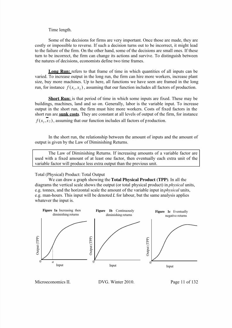
In the short run, the relationship between the amount of inputs and the amount ofoutput is given by the Law of Diminishing Returns.
The Law of Diminishing Returns. If increasing amounts of a variable factor areused with a fixed amount of at least one factor, then eventually each extra unit of thevariable factor will produce less extra output than the previous unit.
Total (Physical) Product: Total OutputWe can draw a graph showing the Total Physical Product (TPP). In all the
diagrams the vertical scale shows the output (or total physical product) in physical units,e.g. tonnes, and the horizontal scale the amount of the variable input in physical units,e.g. man-hours. This input will be denoted L for labour, but the same analysis applieswhatever the input is.
Input
O u t p u t ( T P P )
0
Figure 1a Increasing then
diminishing returns
Input
O u t p u t ( T P P )
0
Figure 1b Continuously
diminishing returns
Input
O u t p u t ( T P P )
0
Figure 1c Eventually
negative returns
a

8/20/2019 ApuntesMicroeconomía II. David Vazquez.pdf
http://slidepdf.com/reader/full/apuntesmicroeconomia-ii-david-vazquezpdf 12/132
Microeconomics II. DVG. Winter 2010. Page 12 of 132
All the shapes in Figure 1 are consistent with the Law of Diminishing Returns.Figure 1a shows what is usually regarded as the normal situation: if there is a zero inputof the variable input, there is no output, so the curve must start at the origin. With the firstfew additions to the variable input, returns increase, so the TPP line gets steeper at first.
The Law tells us that the line will eventually begin to flatten out, as it does after the inputreaches a. In Figure 1b, returns start to diminish from the first unit of input onwards, sothe curve is flattening from the beginning. In both Figures 1a and 1b, the curve flattensout but never turns down – the Law does not say that Total Product will fall. Figure 1cshows the alternative possibility, that TPP does eventually fall.
From now on, we shall analyze the first case, but the same analysis could be donefor the other cases. For convenience we shall think of labor as the variable input anddenote it by L, but the same analysis applies to any variable input. In practice some sortsof labor are not variable in the short run. The standard convention is that exists fixedinput is capital (K) and labor is a variable input (L).
Average Physical ProductFrom the Total, we can derive the Average
Physical Product ( APP), defined as APP = TPP / L.
Geometrically, this is measured by the slope of thestraight line from a particular point on the curve tothe origin, as this is the vertical height (TPP)divided by the horizontal distance ( L).
This rises at first, to a maximum at b, then falls, asshown in the lower part of Figure 2.
2
Marginal Physical ProductWe can also derive the Marginal Physical Product
( MPP). For a unit change in the input, and using Δ as before to denote ‘change in’, this is
L
TPP MPP
Δ
Δ=
)(
If we consider making the change in L smaller andsmaller, MPP becomes
dL
TPPd MPP
)(=
In words, the MPP is the slope of TPP.
In Figure 2, we see that the slope of TPP starts lowand increases as far as a, then it declines
2 This condition corresponds to the total product that has first increasing then diminishing returns (Figure1a). To show the second case (1b) where there is continuously diminishing returns we just need to make thediagram starting from the line plotted by the letter a to the right.
Input (Q)
T P P
0
Figure 2 Total Physical Product, AveragePhysical Product and Marginal
Physical Product
a b
Input (Q)
A
P P ,
M P P
0a b
MPP
APP
c
c

8/20/2019 ApuntesMicroeconomía II. David Vazquez.pdf
http://slidepdf.com/reader/full/apuntesmicroeconomia-ii-david-vazquezpdf 13/132
Microeconomics II. DVG. Winter 2010. Page 13 of 132
continuously but always remains positive. So MPP initially increases then falls.
We can also see the relationship of MPP to APP. Below b, e.g. at a, the tangent is alwayssteeper than the line from the origin, so MPP is greater than APP. At b, the line from theorigin is the tangent, so APP = MPP. After b, e.g at c, the line from the origin is steeper
than the tangent, so MPP is less than APP. Hence the shape of MPP is as shown in the bottom diagram.
An implication is that the marginal product of labor ( L
q MPL
Δ
Δ= ) is assumed to
be a diminishing relationship, as shown below.
L
Q
0
Diminishing marginal
product of labor MPL (lower)
MPL (higher)
q=f(L)
The average product of labor is L
q APL =
An example of a simplified form of a short run production function with two
inputs (capital is fixed) may be the following:
4/320 Lq =
For this production function, the marginal product of labor is:
4/14/1
154
)3(20 −−
== L L
MPL
And the average product of labor is:
4/14/3
2020 −== L
L
L APL
The graphical representation of this production function might be the following:

8/20/2019 ApuntesMicroeconomía II. David Vazquez.pdf
http://slidepdf.com/reader/full/apuntesmicroeconomia-ii-david-vazquezpdf 14/132
Microeconomics II. DVG. Winter 2010. Page 14 of 132
q=20L3/4
L
Q
0
COSTS
Total variable cost (TVC) is the cost of all variable inputs used by the firm (=wL).
Total fixed cost (TFC) is the cost of all fixed inputs used by the firm in the shortrun (=rK).
Total cost (TC) is the sum of TVC and TFC (= wL + rK).
If q is the quantity of output used by the firm, then:
Average Variable Cost = AVC = TVC/q
Average Fixed Cost = AFC = TFC/q
Average Total Cost = ATC = TC/q
q
TFC
q
TVC
q
TFC TVC
q
TC +=
+=
⇒ ATC = AVC + AFC
Marginal cost is the addition to total cost when output rises by a unit.
Because we assume that capital is fixed, and labor is variable, the cost function became the following:
)(
)(
qwf k r
wLk r qTC
+=
+=
Recall that )( L f q = , r is the rental rate of capital and w is the wage rate (the
price of labor).
8/20/2019 ApuntesMicroeconomía II. David Vazquez.pdf
http://slidepdf.com/reader/full/apuntesmicroeconomia-ii-david-vazquezpdf 15/132
Microeconomics II. DVG. Winter 2010. Page 15 of 132
Numerical examples.
Suppose 4/320 Lq = , Fixed costs=500, and wage (w)=10. That will imply,
isolating L, that 3/4
20 ⎟ ⎠
⎞
⎜⎝
⎛
=
q
L
In order to know TC, we know that Total costs= Fixed costs + Variable costs.Total costs, as a function of quantity is the following:
)(
)(
qwf k r
wLk r qTC
+=
+=
3/4
2010500)(
10500
⎟ ⎠ ⎞⎜
⎝ ⎛ +=
+=
qqTC
LTC
Given this function, we can calculate average total cost (divide over q), averagevariable cost (the variable part over q), average fixed cost (the fixed part over q) andmarginal cost (the first derivative of this function with respect to q).
Another example.
21)( qqTC += ,
Then, Fixed costs=1, and variable costs =2
q
⎟⎟ ⎠
⎞⎜⎜⎝
⎛ =
q
q AVC
2
q AVC =
⎟⎟ ⎠
⎞⎜⎜⎝
⎛ =
q AFC
1
qqq
q
q
TC AC +=
+==
11 2
TC MC 2=
ΔΔ=

8/20/2019 ApuntesMicroeconomía II. David Vazquez.pdf
http://slidepdf.com/reader/full/apuntesmicroeconomia-ii-david-vazquezpdf 16/132
Microeconomics II. DVG. Winter 2010. Page 16 of 132
Full condition for profit maximization
Profit is maximized at the output where
• MR = MC ( MR = MC is a necessary condition for profit maximization but is not asufficient condition)
• and MC cuts MR from below (why?), except that the firm will reduce its loss by producing zero output if
• in the short run P < AVC where MR = MC
• and in the long run P < LRAC where MR = LRMC
Output
C o s t s , r e v e n u e
0
Figure 6 Long-run profit maximisation
TC
TR
Total profit
Output0
LRAC
LRMC
QL
PL
MR AR
QL
Qm
Qm
8/20/2019 ApuntesMicroeconomía II. David Vazquez.pdf
http://slidepdf.com/reader/full/apuntesmicroeconomia-ii-david-vazquezpdf 17/132
Microeconomics II. DVG. Winter 2010. Page 17 of 132
LESSON 3: Market structures I, Perfect competition and
elasticity.
Perfect competition.
In the short run, the number of firms is fixed. Price is determined in the market, by the interaction of supply and demand; that is the same to say that firms are pricetakers.
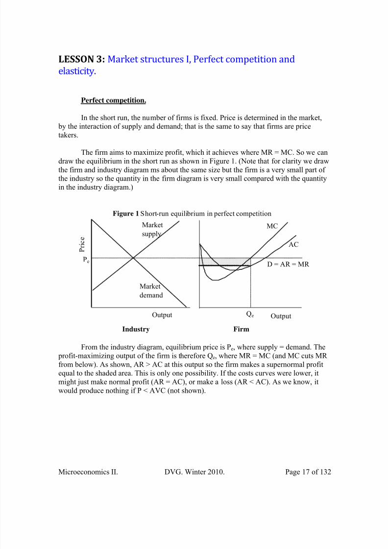
The firm aims to maximize profit, which it achieves where MR = MC. So we candraw the equilibrium in the short run as shown in Figure 1. (Note that for clarity we drawthe firm and industry diagram ms about the same size but the firm is a very small part ofthe industry so the quantity in the firm diagram is very small compared with the quantityin the industry diagram.)
Industry Firm
OutputOutput
P r i c e
Pe
Qe
MC
AC
D = AR = MR
Figure 1 Short-run equilibrium in perfect competition
Market
supply
Marketdemand
From the industry diagram, equilibrium price is Pe, where supply = demand. The profit-maximizing output of the firm is therefore Qe, where MR = MC (and MC cuts MRfrom below). As shown, AR > AC at this output so the firm makes a supernormal profitequal to the shaded area. This is only one possibility. If the costs curves were lower, it
might just make normal profit (AR = AC), or make a loss (AR < AC). As we know, itwould produce nothing if P < AVC (not shown).
8/20/2019 ApuntesMicroeconomía II. David Vazquez.pdf
http://slidepdf.com/reader/full/apuntesmicroeconomia-ii-david-vazquezpdf 18/132
Microeconomics II. DVG. Winter 2010. Page 18 of 132
Profits (π )
TC TR −=π
TR = Total RevenueTC = Total Cost
q AC pq ⋅−=π
Where q AC TC q
TC AC ⋅=⇒=
Under perfect competition, in the long run, 0=π , because additional firms will
enter the market. If there exists some firm making additional profit above the industrialaverage, more firms will enter in the market, driving down economic profits to zero.
In the long run
AC p =
And by profit maximization,
MC MR p ==
Therefore
MC AC =
Numerical Exercise.
Suppose q MC 2.0= . Derive the firm’s supply function.
We know that the profit maximization condition, marginal revenue is equal tomarginal cost. Under perfect competition, price is equal to marginal revenue. Then:
q p 2.0=
?=q
Solve for q,
q p102=
pq 5= , this is the supply function.
If the market price is $10, then
50)10(55 === pq units

8/20/2019 ApuntesMicroeconomía II. David Vazquez.pdf
http://slidepdf.com/reader/full/apuntesmicroeconomia-ii-david-vazquezpdf 19/132
Microeconomics II. DVG. Winter 2010. Page 19 of 132
If the market demand curve is
pQd 506000 −=
Given the market price of $10,
5500)10(506000 =−=d Q
In equilibrium, sd QQ = (total demand is equal to total supply), so we must have
11050
5500= competitive firms in the market in order to supply the required
amount..
Note: Solve equilibrium with linear curves in Varian, Ch. 16, p. 292.
Price elasticity of demand (ed)
The price elasticity of demand is a unit free measure of the responsiveness ofquantity demanded of a good to changes in the price of that good.
goodthatof priceinchange%
goodaof demandedquantityinchange%−=d e
dp
p
Q
dQ
pdp
QdQed ×=−=
/
/
dQdp
Q ped
/
/−=
Q
p
dp
dQed ⋅−= , where
dp
dQ− is the slope of the demand curve.
Proof
The definition of elasticity is
priceinchange percentageThe
demandedquantityinchange percentageThe
Using the Greek letter Δ to denote ‘change in’, P for price and Q for quantity, thiscan be written as
8/20/2019 ApuntesMicroeconomía II. David Vazquez.pdf
http://slidepdf.com/reader/full/apuntesmicroeconomia-ii-david-vazquezpdf 20/132
Microeconomics II. DVG. Winter 2010. Page 20 of 132
P
P
Q
Q
Δ
Δ
This can be re-arranged as
Q
P
Q
PQP
PQ×
Δ
Δ=
×Δ×Δ 1
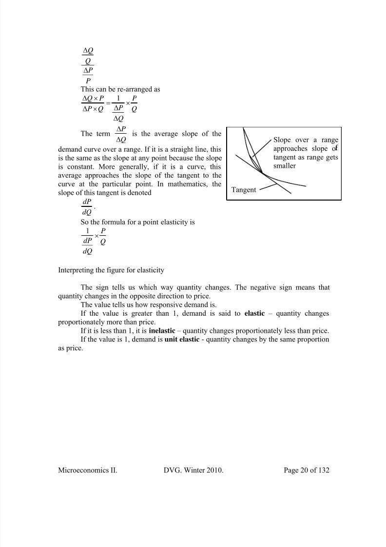
The termQ
P
Δ
Δ is the average slope of the
demand curve over a range. If it is a straight line, thisis the same as the slope at any point because the slopeis constant. More generally, if it is a curve, thisaverage approaches the slope of the tangent to thecurve at the particular point. In mathematics, the
slope of this tangent is denoted
dQ
dP.
So the formula for a point elasticity is
Q
P
dQ
dP ×
1
Interpreting the figure for elasticity
The sign tells us which way quantity changes. The negative sign means thatquantity changes in the opposite direction to price.
The value tells us how responsive demand is.If the value is greater than 1, demand is said to elastic – quantity changes
proportionately more than price.If it is less than 1, it is inelastic – quantity changes proportionately less than price.If the value is 1, demand is unit elastic - quantity changes by the same proportion
as price.
Slope over a rangeapproaches slope otangent as range getssmaller
Tangent

8/20/2019 ApuntesMicroeconomía II. David Vazquez.pdf
http://slidepdf.com/reader/full/apuntesmicroeconomia-ii-david-vazquezpdf 21/132
Microeconomics II. DVG. Winter 2010. Page 21 of 132
At some points on the demand curve, slope of line 1 = slope of line 2. At that point, ed is unity. All points above have own price elasticity of demand greater then unity.Demand is said to be elastic. All points below have own price elasticity of demand lessthan unity, Demand is said to be inelastic.
For the previous example
5500
1050 ⋅−=⋅−=
Q
p
dp
dQed
11
1−=
d
e , therefore is inelastic.

8/20/2019 ApuntesMicroeconomía II. David Vazquez.pdf
http://slidepdf.com/reader/full/apuntesmicroeconomia-ii-david-vazquezpdf 22/132
Microeconomics II. DVG. Winter 2010. Page 22 of 132
LESSON 4: Market structures II, Monopoly, elasticity and
revenue.
Monopoly.
Characteristics:
Single seller, just one firm in an industry. Monopolist’s product is unique, has no close substitutes. There are barriers to entry.
Monopolist’s TR curve:
In the diagram above, the TR curve has been derived from the demand curve. The
TR curve reaches a maxima and MR is zero when demand is unit elastic (e=1).3 When demand is elastic (e>1), as price drops and quantity demanded rises, the TR
also increases. This movement is traced by the green arrows.
Monopolist’s MR curve
3 Recall that by the definition of elasticity, some authors put it as a negative entity, therefore we can say being elastic is e<-1 (in the diagram e>1) or being inelastic is when e>-1.

8/20/2019 ApuntesMicroeconomía II. David Vazquez.pdf
http://slidepdf.com/reader/full/apuntesmicroeconomia-ii-david-vazquezpdf 23/132
Microeconomics II. DVG. Winter 2010. Page 23 of 132
MR < ARThe MR curve lies below to the AR curve.
When demand if inelastic (e<1), as price drops and quantity demanded rises, the
TR decreases. This movement is traced by the brown arrows.
Profit Maximizing condition:
The monopolist’s main objective is to maximize profits. The firm will producethat quantity of output that maximizes its profits.
As seen in the diagram below, the distance between total revenue and total costcurves is maximized when output is Q*.
When output is Q*, the slope of the TR curve equals the slope of the TC curve.
When output is Q*, MR equals MC.
Q* is the profit maximizing level of output for the monopolist.
The profit maximizing output of the monopolist is determined by equatingmarginal revenue with marginal cost.
The equation below is the profit maximizing condition.
MR = MC

8/20/2019 ApuntesMicroeconomía II. David Vazquez.pdf
http://slidepdf.com/reader/full/apuntesmicroeconomia-ii-david-vazquezpdf 24/132
Microeconomics II. DVG. Winter 2010. Page 24 of 132
In the diagram above, the profit maximizing output of the monopolist is Q m. The
price is determined from the demand curve. The monopolist will sell this good at a unit price of pm (this is the maximum he can get, doesn’t make any sense to choose a lower price, but it is assumed the monopolist knows the demand curve –consumer tastes). Thatis the maximum price the buyer is willing to pay. The profit or loss is determined fromthe ATC curve. Is possible ATC to be above AR, but it is operating with a loss, in thiscase, this monopoly might not have sufficient conditions to start to operate (See Varian, p. 431).
Remark.
For a linear (downward sloping) demand function, the slope of the marginal
revenue function is twice the slope of the inverse demand function.
E.g. suppose 0>−= bb
p
b
aq
The inverse demand function
bqa p
qb
a
b
p
−=
−=
Total Revenue
2
)(
bqaq
qbqaq pTR
−=
−=×=
Then, marginal revenue

8/20/2019 ApuntesMicroeconomía II. David Vazquez.pdf
http://slidepdf.com/reader/full/apuntesmicroeconomia-ii-david-vazquezpdf 25/132
Microeconomics II. DVG. Winter 2010. Page 25 of 132
bqaq
TR MR 2−=
Δ
Δ=
q0
a
MR AR=D-2b -b
p
If we want to try a general case for a linear demand function, the following case
might be enlightening: From 0,0,0 >>>−= d cb pd
c
b
aq , get q
c
d
bc
ad p −= ,
2q
c
d q
bc
ad TR −= , and q
c
d
bc
ad MR
2−= .
Numerical Example.
Suppose pQ 506000 −= , and 10== AC MC , Find profit maximization p and q.
q p
q p
50
1120
600050
−=
−=
Total Revenue is price multiplied by quantity
2
50
1120
50
1120
qqq pTR
−=
⎟ ⎠
⎞⎜⎝
⎛ −=×=
Maximizing profit, we need the value of marginal revenue
8/20/2019 ApuntesMicroeconomía II. David Vazquez.pdf
http://slidepdf.com/reader/full/apuntesmicroeconomia-ii-david-vazquezpdf 26/132
Microeconomics II. DVG. Winter 2010. Page 26 of 132
q
TR MR
25
1120
50
2120
−=
−=Δ
Δ=
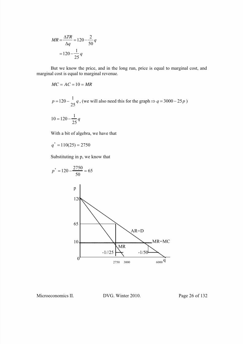
But we know the price, and in the long run, price is equal to marginal cost, andmarginal cost is equal to marginal revenue.
MR AC MC === 10
q p25
1120 −= , (we will also need this for the graph pq 253000 −=⇒ )
q25
1
12010 −=
With a bit of algebra, we have that
2750)25(110* ==q
Substituting in p, we know that
6550
2750120* =−= p
q0
MR
AR=D
-1//25 -1/50
p
10
65
120
30002750 6000
MR=MC
8/20/2019 ApuntesMicroeconomía II. David Vazquez.pdf
http://slidepdf.com/reader/full/apuntesmicroeconomia-ii-david-vazquezpdf 27/132
Microeconomics II. DVG. Winter 2010. Page 27 of 132
The monopolist profit, considering that the average cost is equal to marginal cost,is the following.
151250
)2750(55
)1065(2750
)(
=
=
−=−=
−=
−=
AC pq
ACq pq
TC TRπ
The consumer surplus (we will see that later), is equal to the triangle area abovethe price and below the demand curve.
75625
2/2750)65120(
=
−=CS
Marginal Revenue and Elasticity.
The elasticity of demand measures the responsiveness of the market to quantity produced when prices change. There is a mathematical similarity between the marginalrevenue equation and the formula for elasticity; therefore it will be convenient to showwhat happen to revenue depending of the responsiveness of demand to price changes.
As we saw earlier, our definition of elasticity was the following
Q
p
dp
dQed ⋅−= , where
dp
dQ− is the slope of the demand curve.
From previous paragraphs, we have that Total Revenue q pTR ×= , but we know
that price is a function of quantity )(q p p = (this does not mean that p is multiplying q,
but that p is a function of q, this will be clear with the use of calculus), so
qq pTR ×= )(
We know that Marginal Revenue is the change on total revenue when quantity
changes,4
q
TR MR
Δ
Δ=
4 Assuming continuity and differentiability, marginal changes are translated into differentials.

8/20/2019 ApuntesMicroeconomía II. David Vazquez.pdf
http://slidepdf.com/reader/full/apuntesmicroeconomia-ii-david-vazquezpdf 28/132
Microeconomics II. DVG. Winter 2010. Page 28 of 132
Then, our formulation became the following
))(( qq pq
p MR ×
Δ
Δ=
Preparing the formulation to use product and chain rule, we say that )(q pU = ,
and qV = , so U V V U UV q
p'' +=
Δ
Δ (product rule), and '))(( q
q
pq p
q
p×
Δ
Δ=
Δ
Δ (chain rule,
because q is not constant).
qq p p
pqq
p
qq pq
p MR
Δ
Δ+=
+⋅Δ
Δ=
×Δ
Δ=
)1()1(
))((
With a bit of algebra we want to demonstrate that
⎟ ⎠
⎞⎜⎝
⎛ +=
Δ
Δ+=
ε
11 pq
q
p p MR
How? Let’s try..

8/20/2019 ApuntesMicroeconomía II. David Vazquez.pdf
http://slidepdf.com/reader/full/apuntesmicroeconomia-ii-david-vazquezpdf 29/132
Microeconomics II. DVG. Winter 2010. Page 29 of 132
p p
q
q p
q
pq
q
q p pq
pq
q p pq p
q
p
p
q
q p
q p pq
p
q
p
p
q
q
p
p
q
p
q
p
p
q p
p MR
Δ
Δ+=
Δ
⋅Δ+
Δ
⋅Δ=
Δ
⋅Δ+⋅Δ=
⎟⎟ ⎠
⎞⎜⎜⎝
⎛
⋅Δ
⋅Δ+⋅Δ=
⎟⎟⎟⎟
⎠
⎞
⎜⎜⎜⎜
⎝
⎛
⋅Δ
Δ
⋅Δ⋅Δ+⋅Δ
=
⎟⎟⎟⎟
⎠
⎞
⎜⎜⎜⎜
⎝
⎛
⋅Δ
Δ
+⋅Δ
Δ
=
⎟⎟⎟
⎟
⎠
⎞
⎜⎜⎜
⎜
⎝
⎛
⋅Δ
Δ+=
⎟ ⎠
⎞⎜⎝
⎛ +=
1
11
11
ε
Which is exactly the definition of Marginal revenue •
Now that we know that ⎟ ⎠
⎞⎜⎝
⎛ +=ε
11 p MR , there are some implications. If the
demand curve is inelastic (<-1), the marginal revenue will be positive, if it is unit elastic,marginal revenue is zero, and if the elasticity is greater than -1, marginal revenue will benegative, this is

8/20/2019 ApuntesMicroeconomía II. David Vazquez.pdf
http://slidepdf.com/reader/full/apuntesmicroeconomia-ii-david-vazquezpdf 30/132
Microeconomics II. DVG. Winter 2010. Page 30 of 132
01
01
01
<⇒−>
=⇒−=
>⇒−<
MR
MR
MR
ε
ε
ε
Please have this in mind, because this means the monopolists will decide to
produce a quantity always in the unit elastic or in the elastic part, because that will givehim positive marginal revenues, this means more profit. This diagram at the beginning ofthese notes show the relationship between marginal revenue, elasticity and total revenue.

8/20/2019 ApuntesMicroeconomía II. David Vazquez.pdf
http://slidepdf.com/reader/full/apuntesmicroeconomia-ii-david-vazquezpdf 31/132
Microeconomics II. DVG. Winter 2010. Page 31 of 132
LESSON 5: Market structures III, Monopoly and price
discrimination.
Monopolist’s price discrimination
Price discrimination occurs when a firm charges different prices for a good. Pricediscrimination transfers consumer surplus — the value a consumer receives from a goodminus the price paid — away from buyers and to the firm, thereby increasing themonopoly’s profit. Price discrimination can occur among units of a good, so that largerorders get a discount, or among groups of buyers, so that some buyers pay a lower price.
CS
Profit
MC
Single price monopoly
Output0
AC
P1
MR AR
Q1 Qc
Pc
.
Price discrimination among groups requires that:♦groups of consumers with different willingness to pay exist;♦the members of each group are easily identified;♦and, no resales of the good are made from one group to another.With price discrimination, the group with the high average willingness to pay
pays a high price and the group with the low average willingness to pay pays a low price.

8/20/2019 ApuntesMicroeconomía II. David Vazquez.pdf
http://slidepdf.com/reader/full/apuntesmicroeconomia-ii-david-vazquezpdf 32/132
Microeconomics II. DVG. Winter 2010. Page 32 of 132
Price discrimination by monopoly
Output0
AC
P1
MR AR
Q4 Qc
Pc
CS
Profit
Q3Q2 Q1
Profit from
Price disc.
♦Perfect price discrimination extracts all the consumer surplus by charging eachconsumer the maximum price that he or she is willing to pay for each unit of output purchased. The more perfectly a monopoly can price discriminate, the closer its output isto the competitive level. A perfectly price-discriminating monopoly eliminates all theconsumer surplus, but does not result in a deadweight loss, so it is efficient.
The way the monopolist can discriminate prices is through knowing very welltheir customers, so offering for them exactly the amount of the good at their price inorder to extract their surplus. They need to be careful in order to avoid offering productwith lower price to high-price consumers, for instance, when is offered a bulk sale in aninappropriate place.
Example.
Suppose the monopoly can divide its customers into two groups, say group 1 andgroup 2. The demands are:
22
11
2100
100
pq
pq
−=
−=
For profit maximization
MC MR MC MR =∧= 21
11
2
11111
1111
2100
100
100100
q MR
qqq pTR
q p pq
−=
−==
−=⇒−=

8/20/2019 ApuntesMicroeconomía II. David Vazquez.pdf
http://slidepdf.com/reader/full/apuntesmicroeconomia-ii-david-vazquezpdf 33/132
Microeconomics II. DVG. Winter 2010. Page 33 of 132
Similarly,
22
2
22222
1222
502
1
50
2
1502100
q MR
qqq pTR
q p pq
−=
−==
−=⇒−=
Now, suppose
20== AC MC
For maximizing profit, we need marginal revenue equal to marginal cost, then
40210020 11 =⇒−= qq
305020 22 =⇒−= qq
Then
3560 21 =∧= p p
What are profits? Let’s have two scenarios, one with price discrimination, andanother with no discrimination. First, with price discrimination.
2050
)3040(20)30(35)40(60
)( 212211
21
=
+−+=
+−+=
−+=
−=
qq AC q pq p
TC TRTR
TC TRπ
What if the firm does not discriminate? (both prices should be the same, nosubscript in p)
p
p pqqq
3200
)2100()100(21
−=
−+−=+=
Then

8/20/2019 ApuntesMicroeconomía II. David Vazquez.pdf
http://slidepdf.com/reader/full/apuntesmicroeconomia-ii-david-vazquezpdf 34/132
Microeconomics II. DVG. Winter 2010. Page 34 of 132
q MR
qq pqTR
q p
3
2
3
200
3
1
3
200
3
1
3
200
2
−=
−==
−=
Substituting,
314370
3
2
3
20020 =∧=⇒−= pqq
311633
3
4900
14003
9100
)70(20
3
14370
=
=
−=
−×=
−= TC TRπ
We see that the monopolist will choose to price discriminate whenever he can.
Price discrimination and elasticity
Recall that
⎟ ⎠
⎞⎜⎝
⎛ +=ε
11 p MR
If we have two markets, then
⎟⎟
⎠
⎞⎜⎜
⎝
⎛ +=
1
11
11
ε
p MR and ⎟⎟
⎠
⎞⎜⎜
⎝
⎛ +=
2
22
11
ε
p MR
For profit maximization
2121 MR MR MR MC MR =⇒==
Therefore
8/20/2019 ApuntesMicroeconomía II. David Vazquez.pdf
http://slidepdf.com/reader/full/apuntesmicroeconomia-ii-david-vazquezpdf 35/132
Microeconomics II. DVG. Winter 2010. Page 35 of 132
⎟⎟ ⎠
⎞⎜⎜⎝
⎛ +=⎟⎟
⎠
⎞⎜⎜⎝
⎛ +
⎟⎟ ⎠
⎞⎜⎜⎝
⎛ +
⎟⎟ ⎠
⎞⎜⎜⎝
⎛ +
=
⎟⎟ ⎠
⎞⎜⎜⎝
⎛ +=⎟⎟
⎠
⎞⎜⎜⎝
⎛ +
2
2
1
1
1
2
2
1
2
2
1
1
11
11
11
11
11
11
ε ε
ε
ε
ε ε
p p
p
p
p p
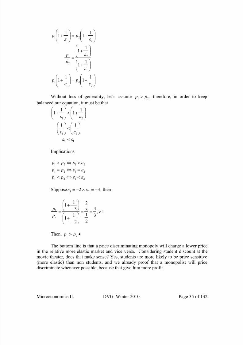
Without loss of generality, let’s assume 21 p p > , therefore, in order to keep
balanced our equation, it must be that
12
21
21
11
11
11
ε ε
ε ε
ε ε
<
⎟⎟ ⎠
⎞⎜⎜⎝
⎛ <⎟⎟
⎠
⎞⎜⎜⎝
⎛
⎟⎟ ⎠
⎞⎜⎜⎝
⎛ +<⎟⎟
⎠
⎞⎜⎜⎝
⎛ +
Implications
2121
2121
2121
ε ε
ε ε
ε ε
<⇔<
=⇔=
>⇔>
p p
p p
p p
Suppose 32 21 −=∧−= ε ε , then
1,3
4
2
13
2
2
11
3
11
2
1 >==
⎟ ⎠
⎞⎜⎝
⎛
−+
⎟ ⎠
⎞⎜⎝
⎛
−+
= p
p
Then, •> 21 p p
The bottom line is that a price discriminating monopoly will charge a lower pricein the relative more elastic market and vice versa. Considering student discount at themovie theater, does that make sense? Yes, students are more likely to be price sensitive(more elastic) than non students, and we already proof that a monopolist will pricediscriminate whenever possible, because that give him more profit.
8/20/2019 ApuntesMicroeconomía II. David Vazquez.pdf
http://slidepdf.com/reader/full/apuntesmicroeconomia-ii-david-vazquezpdf 36/132
Microeconomics II. DVG. Winter 2010. Page 36 of 132
LESSON 6: Market structures IV, Oligopoly.
Oligopoly
Oligopoly is a market structure in which a few (big) firms compete. Each firmconsiders the effects of its actions on the behavior of the others and the actions of theothers on its own profit. Examples of this kind of market structure are oil industry ormovie films companies. So, there is interaction among competitors.
We have so far considered two (polar) extreme cases, the case of perfectcompetition where there are so many firms that each individual firms actions do notaffect the market price, and the case of monopoly, where the single seller has completecontrol over the market price and quantity.
We now consider the intermediate case where there are ‘a few’ firms, each ofwhich has some market power (they influence the price), but not complete control. We
will focus on the simplest structure of oligopoly, that is duopoly, two firms; and we willdo that in an abstract way.
The Cournot model of duopoly
Consider two firms, A and B, each has a marginal cost equal to his average cost of10. Market demand is the following
pqqQ B A −=+= 120 .5
Note that each firm’s profit depends on what the other firm does, that is written in
the following way:
A A B A
A A A
A A A
qqqq
q AC pq
TC TR
10)120( −−−=
−=
−=π
B B B A
B B B
B B B
qqqq
q AC pq
TC TR
10)120( −−−=
−=
−=π
Profit maximization for each firm
B B A A MC MR MC MR =∧=
5 A more general case might be suggested bpaqqQ B A −=+= , whereb
qb
qb
a p B A −−= .

8/20/2019 ApuntesMicroeconomía II. David Vazquez.pdf
http://slidepdf.com/reader/full/apuntesmicroeconomia-ii-david-vazquezpdf 37/132
Microeconomics II. DVG. Winter 2010. Page 37 of 132
Calculating marginal revenue of firm A.
pqq B A −=+ 120
From A point of view pqq B A −−= 120
Inverse demand function for firm A B A qq p −−= 120
Total revenue A B A A A qqq pqTR )120( −−==
Marginal Revenue for firm A B A A qq MR −−= 2120
Set A A MC MR =
B A
B A
B A
2
155
2110
212010
−=
+=
−−=
This is the first ‘reaction’ function, because it is the best response function. Itshows the profit maximizing level of the quantity produced that firm A should choose forevery possible level of quantity produced by firm B.
By symmetry (check!), marginal revenue of firm B A B B qq MR −−= 2120
Set B B MC MR =
A B
A B
A B
2
155
2110
212010
−=
+=
−−=
This is the second ‘reaction’ function. In order to plot a diagram, we need to
consider the values of Aq and B
q . For the case of the first reaction function, when
0= B
q , 55= A
q , and when 0= A
q 110= B
q . For the second reaction function the values
are symmetric.
8/20/2019 ApuntesMicroeconomía II. David Vazquez.pdf
http://slidepdf.com/reader/full/apuntesmicroeconomia-ii-david-vazquezpdf 38/132
Microeconomics II. DVG. Winter 2010. Page 38 of 132
Cournot model
qA 0
55
Firm A’s reaction function
55110
110
Firm B’s reaction function
qB
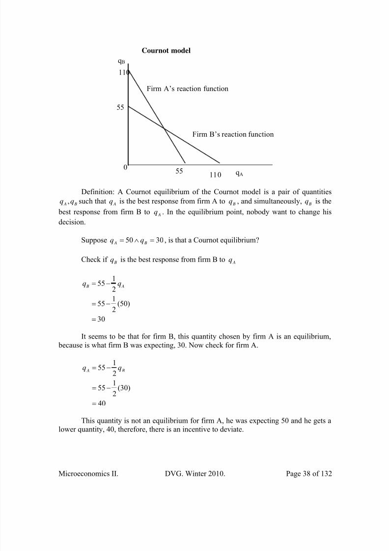
Definition: A Cournot equilibrium of the Cournot model is a pair of quantities B A qq , such that Aq is the best response from firm A to Bq , and simultaneously, Bq is the
best response from firm B to Aq . In the equilibrium point, nobody want to change his
decision.
Suppose 3050 =∧= B A qq , is that a Cournot equilibrium?
Check if Bq is the best response from firm B to Aq
30
)50(2
155
2
155
=
−=
−= A B qq
It seems to be that for firm B, this quantity chosen by firm A is an equilibrium, because is what firm B was expecting, 30. Now check for firm A.
40
)30(2155
2
155
=
−=
−= B A qq
This quantity is not an equilibrium for firm A, he was expecting 50 and he gets alower quantity, 40, therefore, there is an incentive to deviate.

8/20/2019 ApuntesMicroeconomía II. David Vazquez.pdf
http://slidepdf.com/reader/full/apuntesmicroeconomia-ii-david-vazquezpdf 39/132
Microeconomics II. DVG. Winter 2010. Page 39 of 132
Now, suppose3
236
3
236 =∧= B A qq
3
236
)3
236(
2
155
2
155
=
−=
−= B A qq
3
236
)3
236(
2
155
2
155
=
−=
−= A B qq
This pair of quantities chosen are an equilibrium.
Cournot model
qA 0
55
Cournot Equilibrium
55 110
110
qB
36.66
36.66
We can compute Cournot equilibrium, given both reaction functions:
B A qq
2
155 −=
A B qq2
155 −=
Substituting one on the other

8/20/2019 ApuntesMicroeconomía II. David Vazquez.pdf
http://slidepdf.com/reader/full/apuntesmicroeconomia-ii-david-vazquezpdf 40/132
Microeconomics II. DVG. Winter 2010. Page 40 of 132
3
236)
2
155(
2
155 =⇒−−= A A A qqq
And put it back in the second equation we have
3236)
3236(
2155 =⇒−= B B qq , as seen previously.
In order to know the quantity and price equilibrium for the whole market giventhese reaction functions, we put our result in the demand function:
3
173
3
246
1203
173
1203
236
3
236
120
=∧=⇒
−=
−=+
−=+=
Q p
p
p
pqqQ B A
Profits for this equilibrium
1344
)3
23610(
3
236
3
246
=
×−×=
−=
−=
A A A
A A A
q AC pq
TC TRπ
By symmetry,
1344= Bπ too.
The Stackelberg model of duopoly
In the Cournot model, we make the decision at the same time. Now we willassume that one of them is the ‘leader’, and the other is a ‘follower’, this is the onlychange, perhaps trivial, but that will change the outcome.
Suppose firm A is the leader, and B the follower.
Firm A’s decision.

8/20/2019 ApuntesMicroeconomía II. David Vazquez.pdf
http://slidepdf.com/reader/full/apuntesmicroeconomia-ii-david-vazquezpdf 41/132
Microeconomics II. DVG. Winter 2010. Page 41 of 132
A
A
A A
B A
B A
q p
q p
qq p
qq p
pqqQ
2
165
2155120
)2
155(120
120
120
−=
−−=
−−−=
−−=
−=+=
Aq MR −=⇒ 65 (Check!).
55
1065
=
=−
=
A
A
A A
q
q
MC MR
Firm B’s decision.
Firm B’s follows firm A with its optimal response.
5.27
)55(2
155
2
155
=
−=
−= A B qq
In order to know the quantity and price equilibrium for the whole market giventhese reaction functions, we put our result in the demand function:
5.375.82120120
5.825.2755
=−=−=
=+=+=
Q p
qqQ B A
We observe a higher level of output (compared with Cournot equilibrium) andlower price.
What about profits?
5.1512
)5510(555.37
=
×−×=
−=
−=
A A A
A A A
q AC pq
TC TRπ

8/20/2019 ApuntesMicroeconomía II. David Vazquez.pdf
http://slidepdf.com/reader/full/apuntesmicroeconomia-ii-david-vazquezpdf 42/132
Microeconomics II. DVG. Winter 2010. Page 42 of 132
50.756= Bπ (Check!).
Consumers are better off under Stackelberg model, and the ‘leader’ as well, butthe ‘follower’ is worse off.

8/20/2019 ApuntesMicroeconomía II. David Vazquez.pdf
http://slidepdf.com/reader/full/apuntesmicroeconomia-ii-david-vazquezpdf 43/132
Microeconomics II. DVG. Winter 2010. Page 43 of 132
LESSON 7: Game Theory.
Game theory is a tool for studying strategic behavior that can be applied to the
study of different forms of interaction among agents (e.g. oligopoly). This tool helps us tounderstand how people make their assessment of outcomes depending of the actions notonly of themselves, but also considering others.
Games have rules, strategies, payoffs, and an outcome:
♦ Rules specify permissible actions by players.♦Strategies are actions, such as raising or lowering price, output, advertising, or
product quality.♦Payoffs are the profits and losses of the players. A payoff matrix is a table that
shows the payoffs for every possible action by each player.
♦The outcome is determined by the players’ choices.
A “prisoners’ dilemma”.
It is a two-person game. In a one time prisoners’ dilemma game, each player has adominant strategy of cheating, that is, confessing. A dominant strategy occurs when each player has a unique best strategy independent of the other player’s action. The outcome isnot the best equilibrium for the prisoners. The game is the following:
Two people have been arrested on suspicion of having committed a crimetogether, and they are been interrogated in separated cells. Each person has two choices,either confess or not confess.
If both confess, they will be sentenced to jail for 6 years.If both don’t confess, they go to jail for 2 years.If one confess and the other does not, then, the confessor goes free while the non-
confessor goes for 10 years to jail.The utility for the prisoners is a negative unit for each year in jail.
Prisoners' Dilemma Payoff Matrix(Utility for the prisioner)
NC2 C2
NC1 (-2,-2) (-10,0)
C1 (0,-10) (-6,-6)
Prisioner 1
Prisioner 2
Formal description of the game:Players: 1 & 2.
Strategies: 1: { }11,C NC , 2: { }22 ,C NC
Payoffs: Years in prison.
‘Confess’ is a dominant strategy for both players.

8/20/2019 ApuntesMicroeconomía II. David Vazquez.pdf
http://slidepdf.com/reader/full/apuntesmicroeconomia-ii-david-vazquezpdf 44/132
Microeconomics II. DVG. Winter 2010. Page 44 of 132
1C dominates 1 NC for player 1.
2C dominates 2 NC for player 2.
The dominant strategy equilibrium is 21,C C , then both go to jail for six years.
Successive Elimination of dominated strategies:
In the game below, 1a dominates 1b , because in each pair of alternatives, the
choice of a is always better (15 is better than 10, 10 is better than 9, and 18 is better than17).
Successive elimination of dominant strategies(Initial step)
a2 b2 c2
a1 (15,22) (10,7) (18,20)
b1 (10,8) (9,15) (17,1)
c1 (9,10) (15,2) (1,11)
Player 1
Player 2
Formal description of the game:Players: 1 & 2.
Strategies: 1: { }111 ,, cba , 2: { }222 ,, cba
Payoffs: As shown above.
Then, we can get rid of that row.
Successive elimination of dominant strategies(Step 2)
a2 b2 c2
a1 (15,22) (10,7) (18,20)
b1 (10,8) (9,15) (17,1)
c1 (9,10) (15,2) (1,11)
Player 2
Player 1
So, we have a reduced form game.
Successive elimination of dominant strategies(Step 3)
a2 b2 c2
a1 (15,22) (10,7) (18,20)
c1 (9,10) (15,2) (1,11)
Player 2
Player 1

8/20/2019 ApuntesMicroeconomía II. David Vazquez.pdf
http://slidepdf.com/reader/full/apuntesmicroeconomia-ii-david-vazquezpdf 45/132
Microeconomics II. DVG. Winter 2010. Page 45 of 132
We continue applying the same procedure, but now for player 2, in order to see ifthere is a dominant strategy there, we find it
Successive elimination of dominant strategies(Step 4)
a2 b2 c2
a1 (15,22) (10,7) (18,20)
c1 (9,10) (15,2) (1,11)
Player 2
Player 1
The game reduces again.
Successive elimination of dominant strategies(Step 5)
a2 c2
a1 (15,22) (18,20)
c1 (9,10) (1,11)
Player 2
Player 1
We do the same procedure.
Successive elimination of dominant strategies(Step 6)
a2 c2
a1 (15,22) (18,20)
c1 (9,10) (1,11)
Player 2
Player 1
Successive elimination of dominant strategies(Step 7)
a2 c2
a1 (15,22) (18,20)
Player 2
Player 1
Successive elimination of dominant strategies(Step 8)
a2 c2
a1 (15,22) (18,20)
Player 2
Player 1

8/20/2019 ApuntesMicroeconomía II. David Vazquez.pdf
http://slidepdf.com/reader/full/apuntesmicroeconomia-ii-david-vazquezpdf 46/132
Microeconomics II. DVG. Winter 2010. Page 46 of 132
Successive elimination of dominant strategies(Step 9)
a2
a1 (15,22) Dominant
strategyequilibrium
Player 2
Player 1
For this game, we found dominant strategy equilibrium. Equilibrium of this kindmight not exist for all the games.
For instance, the game ‘matching of the pennies’, where two children hold pennies in their hand, they play with them, if both pennies show ‘tail’ or ‘heads’simultaneously, children one wins the penny, if pennies show different face, children twois the one who gets it, in this game, we can not eliminate any strategy, as seen below.
Matching of the pennies(Head or Tail)
H2 T2
H1 (-1,1) (1,-1)
T1 (1,-1) (-1,1)
Player 2
Player 1
Formal description of the game:Players: 1 & 2.
Strategies: 1: { }11 ,T H , 2: { }22 ,T H
Payoffs: Pennies.
Or the game ‘battle of the sexes’, where the story is that a couple go to the movietheater, if both agree in what he wants (Action movie), he gets more utility than her, butif both chooses what she wants (Drama movie), she gets more utility than he. There is arisk of disagreement, when both are worse off in any case, so, one of them needs to‘sacrifice’ a bit in order to get a little bit more than nothing. We can see no dominantstrategy in this game either.
Battle of the sexes(D=choose drama movie, A=choose action movie)
DW AW
DM (1,2) (0,0)
AM (0,0) (2,1)Player 1
Player 2
Formal description of the game:Players: 1 & 2 (Man and Woman).
Strategies: 1: { } M M A D , , 2: { }W W
A D ,
8/20/2019 ApuntesMicroeconomía II. David Vazquez.pdf
http://slidepdf.com/reader/full/apuntesmicroeconomia-ii-david-vazquezpdf 47/132
Microeconomics II. DVG. Winter 2010. Page 47 of 132
Payoffs: Arbitrary utility numbers that represent their preferences.
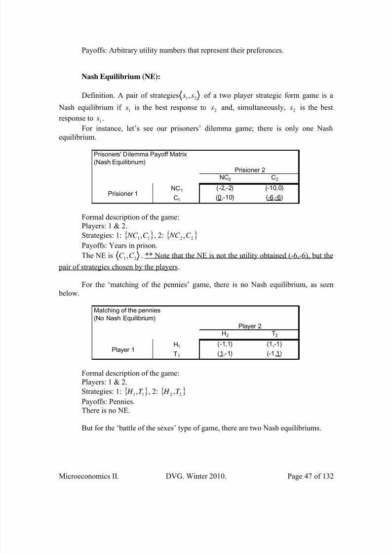
Nash Equilibrium (NE):
Definition. A pair of strategies 21, ss of a two player strategic form game is a Nash equilibrium if 1s is the best response to 2s and, simultaneously, 2s is the best
response to 1s .
For instance, let’s see our prisoners’ dilemma game; there is only one Nashequilibrium.
Prisoners' Dilemma Payoff Matrix(Nash Equilibrium)
NC2 C2
NC1 (-2,-2) (-10,0)
C1 (0,-10) (-6,-6)
Prisioner 2
Prisioner 1
Formal description of the game:Players: 1 & 2.
Strategies: 1: { }11,C NC , 2: { }22 ,C NC
Payoffs: Years in prison.
The NE is 21,C C . ** Note that the NE is not the utility obtained (-6,-6), but the
pair of strategies chosen by the players.
For the ‘matching of the pennies’ game, there is no Nash equilibrium, as seen
below.
Matching of the pennies(No Nash Equilibrium)
H2 T2
H1 (-1,1) (1,-1)
T1 (1,-1) (-1,1)
Player 2
Player 1
Formal description of the game:Players: 1 & 2.
Strategies: 1: { }11 ,T H , 2: { }22 ,T H
Payoffs: Pennies.There is no NE.
But for the ‘battle of the sexes’ type of game, there are two Nash equilibriums.

8/20/2019 ApuntesMicroeconomía II. David Vazquez.pdf
http://slidepdf.com/reader/full/apuntesmicroeconomia-ii-david-vazquezpdf 48/132
Microeconomics II. DVG. Winter 2010. Page 48 of 132
Battle of the sexes(D=choose drama movie, A=choose action movie)
DW AW
DM (1,2) (0,0)
AM (0,0)
(2,1)
Player 2
Player 1
Formal description of the game:Players: 1 & 2 (Man and Woman).
Strategies: 1: { } M M A D , , 2: { }W W
AC ,
Payoffs: Arbitrary utility numbers that represent their preferences.
The NE are W M W M A A D D ,, ∧ .
There is another (anti-coordination) game, which is the so called ‘chicken game’;here there are two Nash equilibriums.
Chicken Game
Swerve2 Straight2
Swerve1 (0,0) (-2,2)
Straight1 (2,-2) (-10,-10)
Player 2
Player 1
Formal description of the game:Players: 1 & 2 .
Strategies: 1: { }11 , Straight Swerve , 2: { }22 , Straight Swerve
Payoffs: Arbitrary utility numbers that represent their preferences.The NE are 2121 ,, Straight SwerveSwerveStraight ∧ .

8/20/2019 ApuntesMicroeconomía II. David Vazquez.pdf
http://slidepdf.com/reader/full/apuntesmicroeconomia-ii-david-vazquezpdf 49/132
Microeconomics II. DVG. Winter 2010. Page 49 of 132
Definition. A pair of strategies 21 , ss is said to be socially optimal if there does
not exist another pair of strategies which makes one player better off without making theother player worse off.
Remarks:
a) A dominant strategy equilibrium is always also a NE (e.g. prisonersdilemma)
b) A NE need not also be a dominant strategy equilibrium (e.g. battle of thesexes)
c) Dominant strategy equilibrium and NE might not be socially optimal. For
instance, prisoner’s dilemma equilibrium 21 ,C C is not socially optimal,
because there is another allocation 21, NC NC where both could be better
off, but on another case, the ‘battle of the sexes’ equilibriums
W M W M A A D D ,, ∧ both are socially optimal.
d) Back to the Cournot equilibrium and Stackelberg equilibrium, those are
types of Nash equilibrium, in this case B A qq , (quantities chosen for
production) are strategies.
Extensive form games.
If we want to include a repeated game over time, or a certain sequence on a game,we might need games in their extensive form. An extensive form game is represented by
a tree, with a unique initial node. Every non-terminal node (that are called informationsets) represents decisions that can be made by players at every point of the game.Terminal nodes determine utility correspondent to each player. For instance, suppose wehave two firms (firm 1 and firm 2). Firm 1 has to decide whether to produce or not produce cars according to certain payoffs. Similarly, Firm 2 has to decide whether it will produce or not produce cars, but after Firm 1’s decision is made. The game is shown inthe following way:

8/20/2019 ApuntesMicroeconomía II. David Vazquez.pdf
http://slidepdf.com/reader/full/apuntesmicroeconomia-ii-david-vazquezpdf 50/132
Microeconomics II. DVG. Winter 2010. Page 50 of 132
Extensive form game1
Cars No Cars
2 2
Cars No Cars Cars No Cars
(5,-2) (10,0) (0,5) (0,0)
The outlined rectangles are called ‘information sets’, inside is written the numberor the name of the player that is making the decision. The numbers inside the brackets
below are the payoffs for player 1 (firm 1) and player 2 (firm 2) respectively.
Another example. ‘Building a home’. Player 1 wants to build a home near to player 2’s home. Player 2 is a bad neighbor, and he threatens to set up a fire on Player’s1’s home if he installs his place near to him. If the fire is started, both places are burned.The extensive form game will look as follows:
Extensive form game'Building a house' 1
Build house No House
2 (2,10)
Fire No fire
(-5,-5) (4,4)
Subgame perfect Nash equilibrium.
A subgame is a subset of the complete game in its extensive form that has aunique initial node and it contains all nodes, terminal and non-terminal, from that point tothe bottom. The nodes below the initial node of a subgame are called successors. Thesubgame perfect Nash Equilibrium (SPNE) is a refinement of a Nash equilibrium in thesense that this solution (a strategy profile) is a Nash equilibrium for every subgame in thecomplete extensive form. The solution to the extensive form game might be done by backward induction. This is done by looking at the information sets at the bottom, andsee if the decision maker would prefer one branch of the three rather than the other. In the
8/20/2019 ApuntesMicroeconomía II. David Vazquez.pdf
http://slidepdf.com/reader/full/apuntesmicroeconomia-ii-david-vazquezpdf 51/132
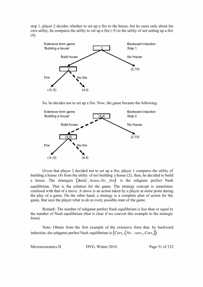
Microeconomics II. DVG. Winter 2010. Page 51 of 132
step 1, player 2 decides whether to set up a fire to the house, but he cares only about hisown utility, he compares the utility to set up a fire (-5) to the utility of not setting up a fire(4).
Extensive form game Backward induction'Building a house' 1 Step 1
Build house No House
2 (2,10)
Fire No fire
(-5,-5) (4,4)
So, he decides not to set up a fire. Now, the game became the following:
Extensive form game Backward induction'Building a house' (4,4) Step 2
Build house No House
(4,4) (2,10)
Fire No fire
(-5,-5) (4,4)
Given that player 2 decided not to set up a fire, player 1 compares the utility of building a house (4) from the utility of not building a house (2), then, he decided to build
a house. The strategies fire Nohouse Build _ , _ is the subgame perfect Nash
equilibrium. That is the solution for the game. The strategy concept is sometimesconfused with that of a move. A move is an action taken by a player at some point duringthe play of a game. On the other hand, a strategy is a complete plan of action for the
game, that says the player what to do at every possible state of the game.
Remark: The number of subgame perfect Nash equilibrium is less than or equal tothe number of Nash equilibrium (that is clear if we convert this example to the strategicform).
Note: Obtain from the first example of the extensive form that, by backward
induction, the subgame perfect Nash equilibrium is 221 , _ , Carscars NoCars .

8/20/2019 ApuntesMicroeconomía II. David Vazquez.pdf
http://slidepdf.com/reader/full/apuntesmicroeconomia-ii-david-vazquezpdf 52/132
Microeconomics II. DVG. Winter 2010. Page 52 of 132
8/20/2019 ApuntesMicroeconomía II. David Vazquez.pdf
http://slidepdf.com/reader/full/apuntesmicroeconomia-ii-david-vazquezpdf 53/132
Microeconomics II. DVG. Winter 2010. Page 53 of 132
Converting an extensive form game to strategic form.
Definition: A strategy for a player is an expectation of an action for each of the players information sets.
In the example above of producing cars or not, the strategies for each player is asfollows:
Players: 1 & 2 (Firm 1 and Firm 2).
Strategies: Player 1: { }11 _ , cars NoCars ,
Player 2:⎪⎭
⎪⎬⎫
⎪⎩
⎪⎨⎧
2222
2222
_ , _ ,, _
, _ ,,,
cars Nocars NoCarscars No
cars NoCarsCarsCars
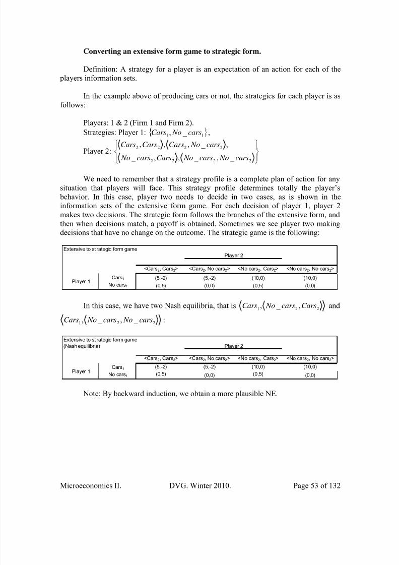
We need to remember that a strategy profile is a complete plan of action for anysituation that players will face. This strategy profile determines totally the player’s
behavior. In this case, player two needs to decide in two cases, as is shown in theinformation sets of the extensive form game. For each decision of player 1, player 2makes two decisions. The strategic form follows the branches of the extensive form, andthen when decisions match, a payoff is obtained. Sometimes we see player two makingdecisions that have no change on the outcome. The strategic game is the following:
Extensive to st rategic form game
<Cars2, Cars2> <Cars2, No cars2> <No cars2, Cars2> <No cars2, No cars2>
Cars1 (5,-2) (5,-2) (10,0) (10,0)No cars1 (0,5) (0,0) (0,5) (0,0)
Player 1
Player 2
In this case, we have two Nash equilibria, that is 221 , _ , Carscars NoCars and
221 _ , _ , cars Nocars NoCars :
Extensive to st rategic form game(Nash equilibria)
<Cars2, Cars2> <Cars2, No cars2> <No cars2, Cars2> <No cars2, No cars2>
Cars1 (5,-2) (5,-2) (10,0) (10,0)
No cars1 (0,5) (0,0) (0,5) (0,0)
Player 2
Player 1
Note: By backward induction, we obtain a more plausible NE.

8/20/2019 ApuntesMicroeconomía II. David Vazquez.pdf
http://slidepdf.com/reader/full/apuntesmicroeconomia-ii-david-vazquezpdf 54/132
Microeconomics II. DVG. Winter 2010. Page 54 of 132
Other ‘refinements’ of Nash equilibrium.
If we convert the extensive form game of ‘building a house’ into a strategic form,we got the following:
Building a house
Fire No Fire
House (-5,-5) (4,4)
No House (2,10) (2,10)
Player 2
Player 1
We can eliminate one of the NE in this game, because one of them is implausible: player two will never choose to set up a fire, the reason is that strategy is not dominated, but is ‘weakly’ dominated by the ‘no fire’ option. So, the plausible Nash equilibrium is
fire Nohouse Build _ , _ .

8/20/2019 ApuntesMicroeconomía II. David Vazquez.pdf
http://slidepdf.com/reader/full/apuntesmicroeconomia-ii-david-vazquezpdf 55/132
Microeconomics II. DVG. Winter 2010. Page 55 of 132
LESSON 8: Consumer theory I. Budget set and preferences.
Model of consumer’s affordability:
A consumer’s choice is limited by what he can afford. He has a given amount ofincome and he cannot change the prices of goods and services he wants to buy. A budget
set is the set of all consumption bundles the consumer can afford to buy. The boundary between the affordable bundles and the unaffordable bundles is the budget line. SupposeTom consumes only movies and popcorn (which are good goods, not bads). In thediagram below, OAB is his budget set and AB is his budget line.
The Equation of the budget line
pX = Price of movies in $ per movie. pY = Price of popcorn in $ per bag.QX = Quantity of movies.QY = Quantity of popcorn.M = Income.
Tom spends all his income on movies and popcorn.Expenditure = Income
M Q pQ pY Y X X
=+
If Tom spends all his income on movies, the maximum number of movies he canwatch is
( ) OB p
M Q
X
Max X ==
(Put QY = 0 in the budget equation.)

8/20/2019 ApuntesMicroeconomía II. David Vazquez.pdf
http://slidepdf.com/reader/full/apuntesmicroeconomia-ii-david-vazquezpdf 56/132
Microeconomics II. DVG. Winter 2010. Page 56 of 132
If Tom spends all his money on popcorn, the maximum quantity of popcorn hecan buy is
( ) OA p
M Q
Y
Y ==max
(Put QX = 0 in the budget equation.)
Slope of the budget line
X = number of movies.Y = number of bags of popcorn.
Absolute Slope of budget line AB =OB
OA
=
X
Y
p M
p M −
= M
p
p
M X
Y
×−
=Y
X
p
p−

8/20/2019 ApuntesMicroeconomía II. David Vazquez.pdf
http://slidepdf.com/reader/full/apuntesmicroeconomia-ii-david-vazquezpdf 57/132
Microeconomics II. DVG. Winter 2010. Page 57 of 132
The slope of the budget line is the ratio of prices of movies and popcorn.
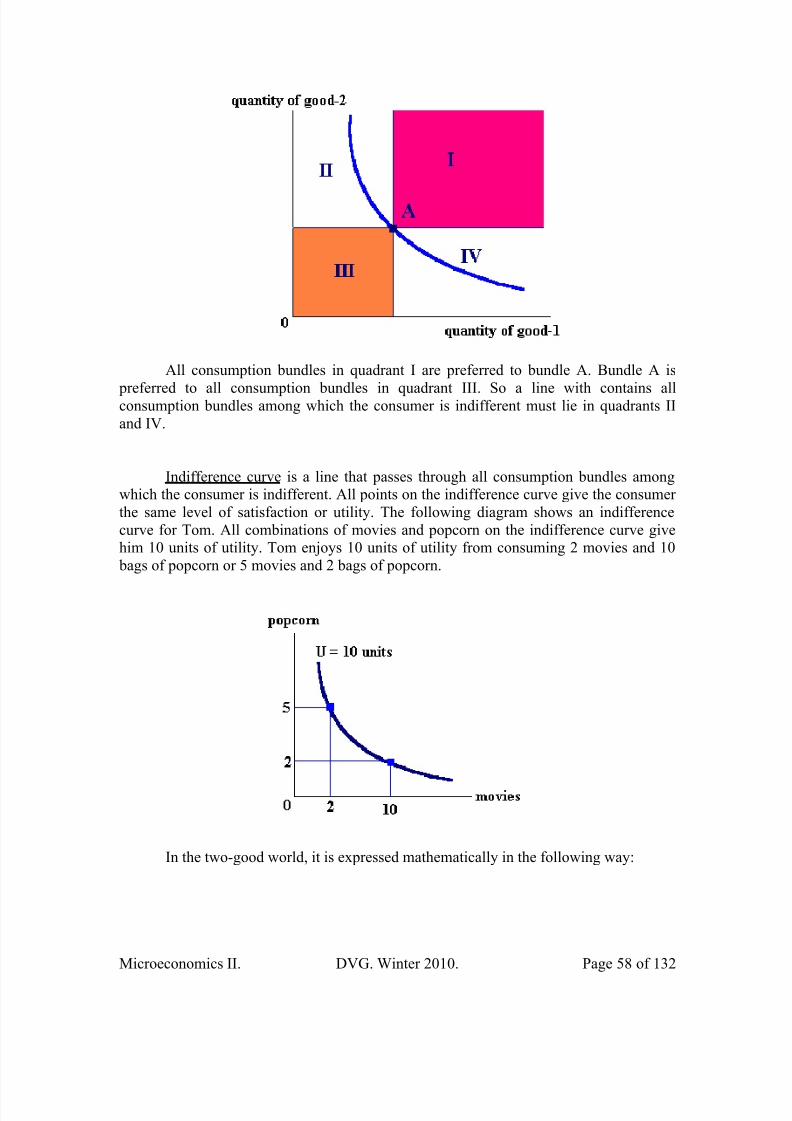
Indifference Curves and Consumer preferences:
Consumers can sort all possible combinations of goods into 3 categories: preferred, not preferred and indifferent. To make a model of consumer’s preferences wemake the following assumptions or axioms:
(1) Axiom of Greediness: More quantity of a “good” good is preferred to lessquantity. This axiom can be shown by the convexity of the upper level sets of theindifference curve.
(2) Axiom of reflexivity: For two identical bundles, one bundle is as good as
the other. One is a reflection of the other.
(3) Axiom of completeness: For two distinct consumption bundles A and B,either the consumer prefers A to B, or prefers B to A, or is indifferent between the two.There is not paralysis by analysis.
(4) Axiom of transitivity: For three consumption bundles A,B and C; if theconsumer prefers A to B and prefers B to C; it must be the case that he prefers A to C.
(5) Axiom of diminishing marginal rate of substitution. This axiom may beexpressed by (strict) monotonicity.6
Now consider a two good world (PLEASE NOTE THAT AXIS ARE VERYDIFFERENT THAN DEMAND AND SUPPLY DIAGRAMS). Plot the quantity of good1 on the horizontal axis and the quantity of good 2 on the vertical axis. Each point of the positive quadrant is some combination of goods 1 and 2. Point A is a consumption bundlewhich contains Q1 quantity of good 1 and Q2 quantity of good 2. Drop a vertical and ahorizontal line through point A thus dividing the consumption space into four quadrants.
6 Monotonicity guarantees that indifference curves are not ‘upward’ sloping. A weaker assumption such as‘local non-satiation’ might be used as well (it rules out fat indifference curves), and it might introduce‘bads’ in the analysis, not only ‘goods’.
8/20/2019 ApuntesMicroeconomía II. David Vazquez.pdf
http://slidepdf.com/reader/full/apuntesmicroeconomia-ii-david-vazquezpdf 58/132
Microeconomics II. DVG. Winter 2010. Page 58 of 132
All consumption bundles in quadrant I are preferred to bundle A. Bundle A is
preferred to all consumption bundles in quadrant III. So a line with contains allconsumption bundles among which the consumer is indifferent must lie in quadrants IIand IV.
Indifference curve is a line that passes through all consumption bundles amongwhich the consumer is indifferent. All points on the indifference curve give the consumerthe same level of satisfaction or utility. The following diagram shows an indifferencecurve for Tom. All combinations of movies and popcorn on the indifference curve givehim 10 units of utility. Tom enjoys 10 units of utility from consuming 2 movies and 10 bags of popcorn or 5 movies and 2 bags of popcorn.
In the two-good world, it is expressed mathematically in the following way:

8/20/2019 ApuntesMicroeconomía II. David Vazquez.pdf
http://slidepdf.com/reader/full/apuntesmicroeconomia-ii-david-vazquezpdf 59/132
Microeconomics II. DVG. Winter 2010. Page 59 of 132
1
21211
1
),(),(
x
x xu x x xu
x
U
Δ
−Δ+=
Δ
Δ
The slope of the indifference curve is the marginal rate of substitution (MRS).It is the quantity of popcorn Tom is willing to give up to watch another movie and keephis total utility the same. It is the ratio of marginal utilities.
Marginal Utility of movies = 1 MU
Marginal Utility of popcorn = 2 MU
11 x MU Δ = Total addition to satisfaction from consuming 1 xΔ movies.
22 x MU Δ = Total addition to satisfaction from consuming 2 xΔ popcorn.
When Tom moves from one point of his indifference curve to another, he gives upone good for another. His total satisfaction or (change in) utility does not alter.
0),(),( 22121211 =Δ+Δ=Δ x x x MU x x x MU U
Rearranging, we have that
),(
),(),(
212
211
1
221
x x MU
x x MU
x
x x x MRS −=
Δ
Δ=
This is the slope of Tom’s indifference curve or the marginal rate of substitution.It is negative. To watch more movies, Tom must give up some popcorn to remainindifferent even as his consumption of a movie rises.
Absolute slope of indifference curves:
2
1slope MU
MU =
As consumption of movies rises, the slope of the indifference curve falls, or the
marginal rate of substitution decreases. This is because Tom is willing to give up lessquantity of popcorn for each additional movie, and at the same time remain indifferent, ashis movie consumption rises. This is called the law of diminishing marginal rate of
substitution.

8/20/2019 ApuntesMicroeconomía II. David Vazquez.pdf
http://slidepdf.com/reader/full/apuntesmicroeconomia-ii-david-vazquezpdf 60/132
Microeconomics II. DVG. Winter 2010. Page 60 of 132
Tom’s indifference curve is steeper at point A than at point B. The marginal rateof substitution is higher at point A than at point B. At point A, Tom is willing to sacrificemore popcorn for one more movie.

8/20/2019 ApuntesMicroeconomía II. David Vazquez.pdf
http://slidepdf.com/reader/full/apuntesmicroeconomia-ii-david-vazquezpdf 61/132
Microeconomics II. DVG. Winter 2010. Page 61 of 132
LESSON 9: Consumer theory I. Utility functions and
optimization.
Model of consumer’s Optimal Choice.
Consumer’s optimal choice depends upon the following:
What the consumer wants, likes or dislikes. This is modeled by theconsumer’s indifference curve.
What the consumer can afford. This is modeled by the consumer’s budgetline.
Optimum Choice:
Optimum choice refers to that consumption bundle which the consumer finallychooses. This is the optimum consumption bundle. The objective of the consumer is tomaximize his utility given his budget set. The consumer will finally choose to buy the best, affordable consumption bundle. The optimum consumption bundle is the consumer
equilibrium.
The best affordable consumption bundle has the following properties:
Condition (1): The optimum consumption bundle is on the budget line.Condition (2): The optimum consumption bundle is on the highest
attainable indifference curve.
In the following diagram the quantity of popcorn (Y) is measured along thevertical axis and the quantity of movies (X) is measured along the horizontal axis. Thediagram illustrates Tom’s preferences and affordability.

8/20/2019 ApuntesMicroeconomía II. David Vazquez.pdf
http://slidepdf.com/reader/full/apuntesmicroeconomia-ii-david-vazquezpdf 62/132
Microeconomics II. DVG. Winter 2010. Page 62 of 132
Consumption bundle A is the optimum consumption bundle. It represents Tom’s best affordable consumption bundle or his consumer equilibrium. While balancing whathe wants with what he can afford, Tom will choose to watch Xo movies and Yo bags of popcorn. The consumer equilibrium is on the budget line. At this point, Tom’sindifference curve is tangent to his budget line. In other words, the slope of the
indifference curve is exactly equal to the slope of the budget line.
Properties of Consumer Equilibrium:
It is on the budget line. It is on the highest attainable indifference curve.
At the optimum consumption bundle A:
Condition (1): Consumer’s total income = total expenditure.
2211 x p x pm +=
Condition (2): The |slope| of the indifference curve = The |slope| of
the budget line.
The |slope| of the indifference curve =2
1
MU
MU −
The |slope| of the budget line =2
1
p
p−
At the optimum choice:
2
1
2
1
p
p
MU
MU =
OR
2
2
1
1
p
MU
p
MU =
The marginal utility per dollar spend on movies is exactly equal to the marginalutility per dollar spend on popcorn.
Algebraic utility maximization
Assuming that we have given prices p1 and p2, and a utility function from the
consumption of goods x1 and x2 with a budget constraint m x p x p =+ 2211 , we want to
maximize our utility given our budget:
8/20/2019 ApuntesMicroeconomía II. David Vazquez.pdf
http://slidepdf.com/reader/full/apuntesmicroeconomia-ii-david-vazquezpdf 63/132
Microeconomics II. DVG. Winter 2010. Page 63 of 132
m x p x p x xu x x =+ 221121, ),(max21
This is a constrained maximization problem. We can put the constraint within the problem with the following procedure:
m x p x p =+ 2211
)( 121
2
1
2
2 x x x p
p
p
m x =−=⇒
Then, our problem became
( ))(,max,max 1211
2
1
2
1 11 x x xu x
p
p
p
m xu x x ⇔⎟⎟
⎠
⎞⎜⎜⎝
⎛ −
We can solve this problem as an unconstrained maximization problem, or as aconstrained maximization problem. Let’s do the unconstrained first.
To maximize the function, first take differentials (using additive and chain rule)and equate those to zero:
( ) ( )0
)(,)(,
1
2
2
121
1
121
1
=∂
∂+
∂
∂=
∂
∂
dx
dx
x
x x xU
x
x x xU
x
U
The derivative of the inside of the function with respect to the second term:
2
1
1
2
p
p
dx
dx−=
Then

8/20/2019 ApuntesMicroeconomía II. David Vazquez.pdf
http://slidepdf.com/reader/full/apuntesmicroeconomia-ii-david-vazquezpdf 64/132
Microeconomics II. DVG. Winter 2010. Page 64 of 132
( ) ( )
( ) ( )
( ) ( )
( )
( )
),(),(
),(
)(,
)(,
)(,)(,
)(,)(,
0)(,)(,
212,1
2
1
212
211
2
1
2
121
1
121
2
1
2
121
1
121
1
2
2
121
1
121
1
2
2
121
1
121
x x MRS p
p
x x MU
x x MU
p
p
x
x x xU
x
x x xU
p p
x x x xU
x x x xU
dx
dx
x
x x xU
x
x x xU
dx
dx
x
x x xU
x
x x xU
==
=
∂
∂∂
∂
⎟⎟ ⎠ ⎞⎜⎜
⎝ ⎛ −
∂∂−=
∂∂
∂
∂−=
∂
∂
=∂
∂+
∂
∂
We can also solve also this problem using the Lagrange method
m x p x p x xu x x =+ 221121, ),(max21
The Lagrangian is as follows:
)(),(),,( 22112121 m x p x p x xu x x L −+−= λ λ
F.O.C.
0),(
1
1
*
2
*
1
1
=−∂
∂=
∂
∂ p
x
x xu
x
Lλ (1)
0),(
2
2
*2
*1
2
=−∂
∂=
∂
∂ p
x
x xu
x
Lλ (2)
0*
22
*
11 =−+=∂
∂m x p x p
L
λ (3)
By (3) we know that the constraint should be binding, and solving (1) and (2), wehave that our marginal rate of substitution will be equal to the factor price ratio:
2
12
*
2
*
11
1
*
2
*
1 ),(0
),( p
x
x xu p
x
x xuλ λ −
∂
∂==−
∂
∂

8/20/2019 ApuntesMicroeconomía II. David Vazquez.pdf
http://slidepdf.com/reader/full/apuntesmicroeconomia-ii-david-vazquezpdf 65/132
Microeconomics II. DVG. Winter 2010. Page 65 of 132
( )
( )
),(),(),(
,
,
212,1
2
1
212
211
2
1
2
*2
*1
1
*
2
*
1
x x MRS p p
x x MU x x MU
p
p
x
x xU
x
x xU
==
=
∂
∂
∂
∂
λ
λ
Which is the same result that we get by unconstrained maximization.
The material shown above will be helpful to understand various theories ofconsumption and later on the concept of general equilibrium.
For instance, from the problem m x p x p x x x xu x x =++= 22112121, 32),(max21
, get
from both methods that2
1212,1
32),(
p p x x MRS == , and from the problem
1054),(max 212121, 21=+= x x x x x xu x x , get that
5
4),(
1
2212,1 ==
x
x x x MRS , and in the
optimal4
5*
1 = x and 1*
2 = x .
Example: Maximizing a Cobb-Douglas utility function:
We can solve this problem using the Lagrange method
m x p x p x x d c
x x =+ 221121, 21max
The Lagrangian is as follows:
)(),,( 22112121 m x p x p x x x x L d c −+−= λ λ
F.O.C.
0121
1
1
=−=∂
∂ − p xcx
x
L d cλ (1)
02
1
21
2
=−=∂
∂ − p xdx
x
L d cλ (2)
8/20/2019 ApuntesMicroeconomía II. David Vazquez.pdf
http://slidepdf.com/reader/full/apuntesmicroeconomia-ii-david-vazquezpdf 66/132
Microeconomics II. DVG. Winter 2010. Page 66 of 132
0*
22
*
11 =−+=∂
∂m x p x p
L
λ (3)
Solving (1) and (2), we have that our marginal rate of substitution will be equal tothe factor price ratio:
2
1
1
2
2
1
1
21
21
1
p
p
dx
cx
p
p
xdx
xcxd c
d c
=
=−
−
λ
λ
We get the value of one of the terms with respect to the other
1
2
12 x
cp
dp x =
Substituting in (3)
mc
d x p
m xc
dp x p
m xcp
dp p x p
=⎟ ⎠
⎞⎜⎝
⎛ +
=⎟ ⎠
⎞⎜⎝
⎛ +
=⎟⎟ ⎠
⎞⎜⎜⎝
⎛ +
111
11
11
1
2
1211
1
*
1 p
m
d c
c x ⎟
⎠
⎞⎜⎝
⎛
+=⇒
And by symmetry:
2
*
2 p
m
d c
d x ⎟
⎠
⎞⎜⎝
⎛
+=∴
We can try to solve this problem either converting this to a monotonictransformation (See Varian, p. 93), or using unconstrained maximization (Try!!).
Examples of utility functions
Indifference curves from utility
8/20/2019 ApuntesMicroeconomía II. David Vazquez.pdf
http://slidepdf.com/reader/full/apuntesmicroeconomia-ii-david-vazquezpdf 67/132
Microeconomics II. DVG. Winter 2010. Page 67 of 132
Suppose we have an utility function of the following form 2121 ),( x x x xu = . We
arbitrarily assign a constant value k to this relationship in order to know how related one
of the variables with respect to the other is. Then, if1
221 x
k x x xk =⇒= . If we want to
know the shape of this function, constructing a two axis diagram, with 1 x in the horizontal
axis, and conversely 2 x on the vertical axis we have the following:
Graph (xxx page 60 Varian)
Now let’s consider other utility function of the following form 2
2
2
121 ),( x x x xv = .
We can put this function with a bit of algebra in the following way 2
2121 )(),( x x x xv = .
But we can express this v function, related with the previous u one.2
2121)),((),( x xu x xv = , so this can be expressed in the following way 2
21),( x xu= , the
square of the u function. We observe that v is a monotonic transformation of u, then theshape of this function will be exactly the same as u, with the only difference that thevalues assigned to them will be higher in that (squared) proportion (1,2,3,…; 1,2,9,…), but both functions order a pair of bundles in the same (progressive) way. This is basic fora utility function, which is the transitive property of the indifference curve.
Perfect substitutes.
When a consumer is willing to substitute one of the goods for another at a one-to-one rate, we have the following function
2121 ),( x x x xu += .7
But if this relationship is different than one-to-one, in general
2121 ),( bxax x xu += (Check the shape of the graph!).8
Perfect complements.
Lets use an example. Suppose we want to say that the utility that gives a pair ofgoods is the less utility we can get from any of those goods (e.g. a pair of shoes, getting
another shoe without its pair is useless). This is expressed in the following way
{ }2121 ,min),( x x x xu =
7 To plot this graph, lets assume 21 x xu += , in the y axis the first point is the distance u .
8 Then 12 xb
ab
u x += .

8/20/2019 ApuntesMicroeconomía II. David Vazquez.pdf
http://slidepdf.com/reader/full/apuntesmicroeconomia-ii-david-vazquezpdf 68/132
Microeconomics II. DVG. Winter 2010. Page 68 of 132
For instance, if one shoe give us 1 unit of utility, and if we get 10 right foot shoes,
and 10 left ones, the utility is (10,10), and the utility function ( { }10,10min ) tells us that
the utility is 10. Adding only one left shoe, that is (11,10), the utility function
( { }10,11min ) tells us that the utility is 10 as well, because there is no benefit in getting
that shoe without its pair (include a graph xxx).In general, there might be different than one-to-one relationships among the
perfect complements, that is said
{ }2121 ,min),( bxax x xu =
Where a and b are positive numbers that indicate such proportions in which goodsare consumed.
Quasilinear preferences
When the consumer considers an increasing (decreasing) utility proportion fromonly one of the two goods chosen (in two-good consumer space), we say that
2121 )(),( x xvk x xu +==
Where )( 1 xv can be a transformation of the variable 1 x (logarithm:
2121 )ln(),( x x x xu += , root: 2121 ),( x x x xu += , etc.). See page 63, Varian.
Cobb-Douglas Preferences
A very used form of a utility function is the following
d c x x x xu 2121 ),( =
Where c and d are positive numbers describing consumer’s preferences.Depending of the values of the superscripts, the preferences take different shapes.
Graph (xxx page 64, Varian).
The examples just given are 21
22
1
121 ),( x x x xu = , and 54
25
1
121 ),( x x x xv =
A convenient monotonic transformation of the Cobb-Douglas utility functionhappens when we apply logarithms to both sides of the equation:
2121
2121
2121
lnln),(
)ln()),(ln(
),(
xd xc x xv
x x x xu
x x x xu
d c
d c
+=
=
=

8/20/2019 ApuntesMicroeconomía II. David Vazquez.pdf
http://slidepdf.com/reader/full/apuntesmicroeconomia-ii-david-vazquezpdf 69/132
Microeconomics II. DVG. Winter 2010. Page 69 of 132
An example for any of this can be done, so a use of logs are introduced. Thismonotonic transformation of the Cobb-Douglas utility function will be convenient for itsuse later on.

8/20/2019 ApuntesMicroeconomía II. David Vazquez.pdf
http://slidepdf.com/reader/full/apuntesmicroeconomia-ii-david-vazquezpdf 70/132
Microeconomics II. DVG. Winter 2010. Page 70 of 132
LESSON 10: Intertemporal Choice.
Intertemporal budget set.
A part of consumer theory in regards to choice, including a dynamic framework,is the intertemporal choice, which is consumer’s choice over more than one period oftime.
Suppose we consider a framework where the consumer lives two periods of time,say period 1 and period 2:
• The consumer has income 1m in period 1 and 2m in period 2.
• The consumer can borrow or lend money at the money market at interest rate r inthe following way:
o If the consumer borrows $x amount of money in period 1, she has to pay back x(1+r ) in period 2.
o If the consumer lends $y amount of money in period 1, she gets backy(1+r ) in period 2.
• The consumer can allocate his income in the following way:
o He has a disposable income of 1m in period 1 and 2m in period 2.
o The maximum amount she can lend in period 1 is 1m , and she can get
back 1m (1+r ) in period 2.
o The maximum amount she can borrow in period 1 isr
m
+12 , as she needs to
pay back 22 )1(
1mr
r
m=+×
+in period 2 (there is not unlimited borrowing
in this framework).
In order to construct a diagram, we need to know for sure the two intercepts:
• Note that the maximum amount the consumer can consume in period 1 is
equal tor
mm
++
1
21
• And the maximum amount the consumer can consume in period 2 is equalto 21 )1( mr m ++ , as we see below.
• The slope of the budget set is
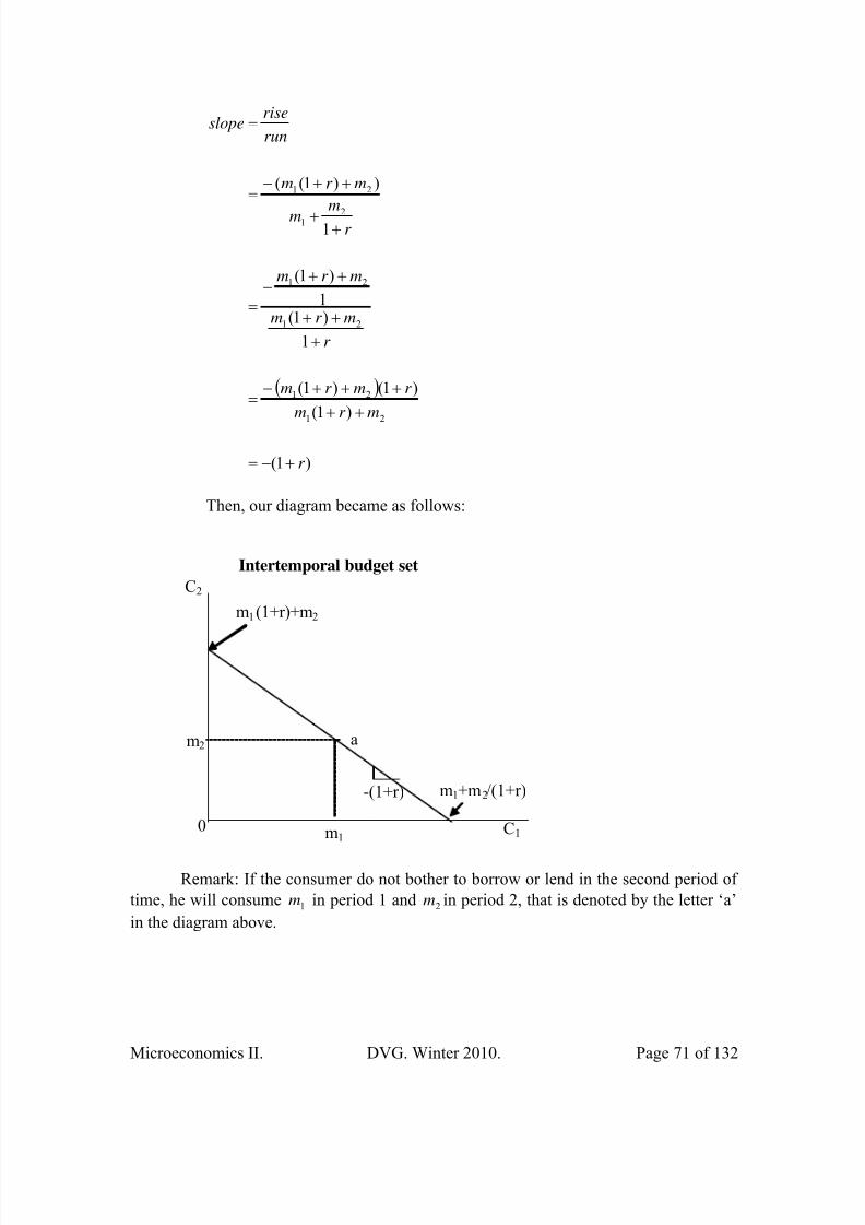
8/20/2019 ApuntesMicroeconomía II. David Vazquez.pdf
http://slidepdf.com/reader/full/apuntesmicroeconomia-ii-david-vazquezpdf 71/132
Microeconomics II. DVG. Winter 2010. Page 71 of 132
( )
)1(
)1(
)1()1(
1
)1(1
)1(
1
))1((
21
21
21
21
21
21
r
mr m
r mr m
r
mr m
mr m
r
mm
mr m
run
riseslope
+−=
++
+++−=
+
++
++−
=
++
++−=
=
Then, our diagram became as follows:
Intertemporal budget set
0
m1(1+r)+m2
C2
a
-(1+r)
C1 m1
m2
m1+m2/(1+r)
Remark: If the consumer do not bother to borrow or lend in the second period of
time, he will consume 1m in period 1 and 2m in period 2, that is denoted by the letter ‘a’
in the diagram above.
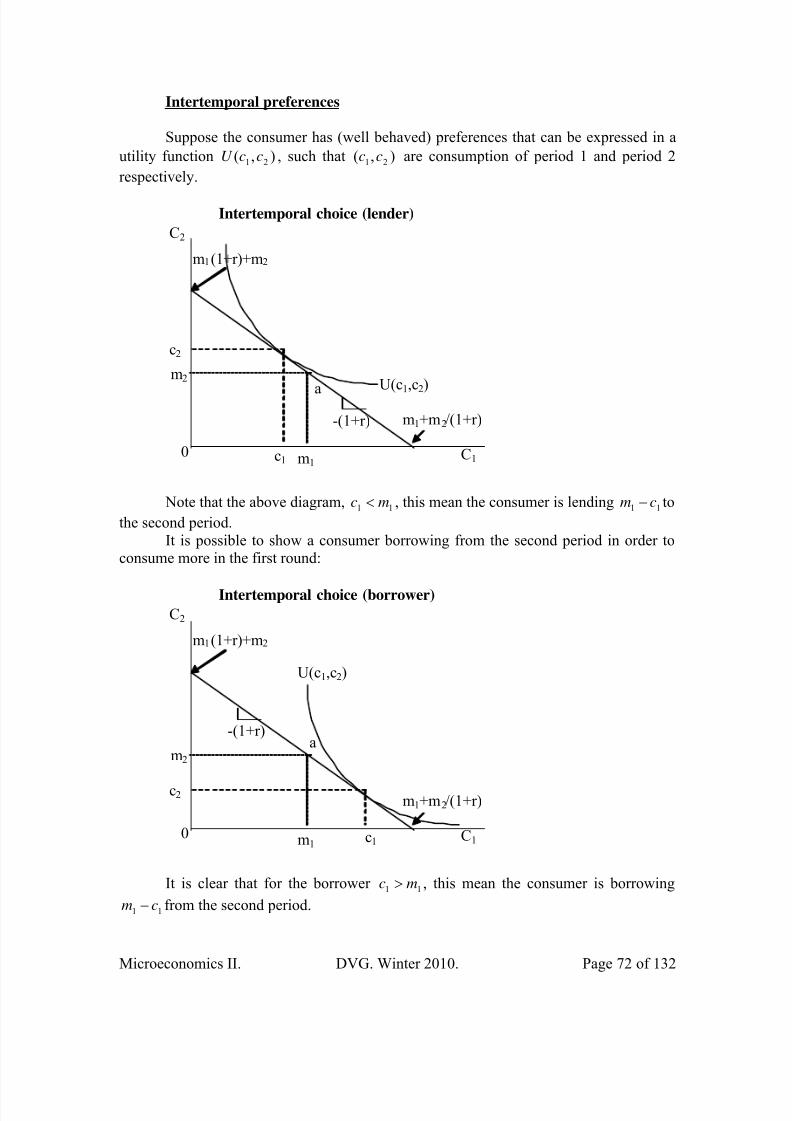
8/20/2019 ApuntesMicroeconomía II. David Vazquez.pdf
http://slidepdf.com/reader/full/apuntesmicroeconomia-ii-david-vazquezpdf 72/132
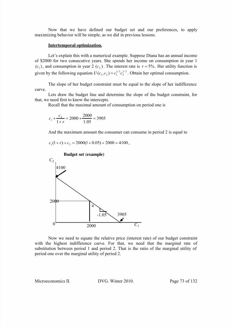
8/20/2019 ApuntesMicroeconomía II. David Vazquez.pdf
http://slidepdf.com/reader/full/apuntesmicroeconomia-ii-david-vazquezpdf 73/132
Microeconomics II. DVG. Winter 2010. Page 73 of 132
Now that we have defined our budget set and our preferences, to applymaximizing behavior will be simple, as we did in previous lessons.
Intertemporal optimization.
Let’s explain this with a numerical example. Suppose Diana has an annual incomeof $2000 for two consecutive years. She spends her income on consumption in year 1
)( 1c , and consumption in year 2 )( 2c . The interest rate is %5=r . Her utility function is
given by the following equation 2/1
2
2/1
121 ),( ccccU = . Obtain her optimal consumption.
The slope of her budget constraint must be equal to the slope of her indifferencecurve.
Lets draw the budget line and determine the slope of the budget constraint, forthat, we need first to know the intercepts.
Recall that the maximal amount of consumption on period one is
390505.1
200020001
21 =+=
++
r
cc
And the maximum amount the consumer can consume in period 2 is equal to
41002000)05.01(2000)1( 21 =++=++ cr c ,
Budget set (example)
0
4100
C2
a
-1.05
C1 2000
2000
3905
Now we need to equate the relative price (interest rate) of our budget constraintwith the highest indifference curve. For that, we need that the marginal rate ofsubstitution between period 1 and period 2. That is the ratio of the marginal utility of period one over the marginal utility of period 2.
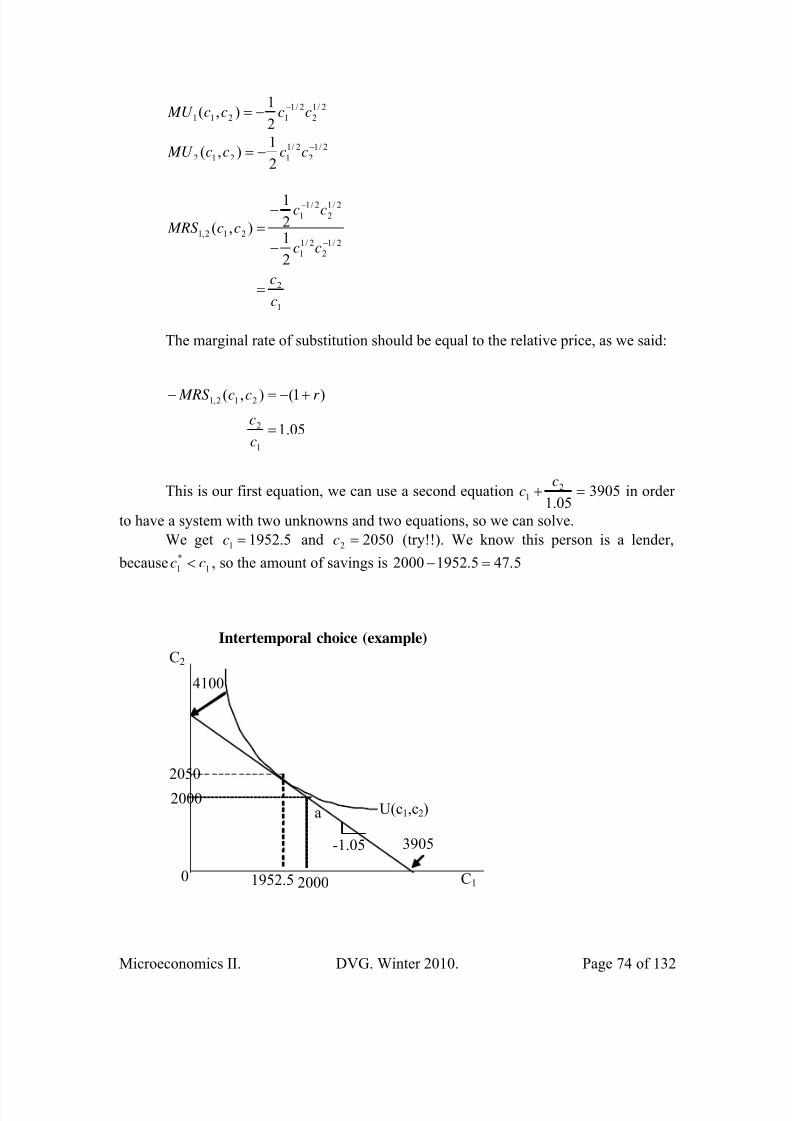
8/20/2019 ApuntesMicroeconomía II. David Vazquez.pdf
http://slidepdf.com/reader/full/apuntesmicroeconomia-ii-david-vazquezpdf 74/132
Microeconomics II. DVG. Winter 2010. Page 74 of 132
2/1
2
2/1
12112
1),( cccc MU −−=
2/1
2
2/1
12122
1),( −−= cccc MU
1
2
2/12
2/11
2/1
2
2/1
1
212,1
2
12
1
),(
c
c
cc
cc
cc MRS
=
−
−=
−
−
The marginal rate of substitution should be equal to the relative price, as we said:
05.1
)1(),(
1
2
212,1
=
+−=−
c
c
r cc MRS
This is our first equation, we can use a second equation 390505.12
1 =+ c
c in order
to have a system with two unknowns and two equations, so we can solve.
We get 5.19521 =c and 20502 =c (try!!). We know this person is a lender,
because 1
*
1 cc < , so the amount of savings is 5.475.19522000 =−
Intertemporal choice (example)
0
4100
C2
a
-1.05
C1 2000
2000
3905
U(c1,c2)
2050
1952.5

8/20/2019 ApuntesMicroeconomía II. David Vazquez.pdf
http://slidepdf.com/reader/full/apuntesmicroeconomia-ii-david-vazquezpdf 75/132
Microeconomics II. DVG. Winter 2010. Page 75 of 132
LESSON 11: Uncertainty.
The act of choice and uncertainty
We relax the discrete notion of choice (either preferring good X to good Y andnot the other way around), with a broader scope of choice including probabilities. Theconsumer now will be interested with the probability distribution of choices amonggoods. A probability to each outcome that results from the act of choice will beassociated then.
The structure of our problems, that use standard utility function that supposedlydescribes consumer’s preferences, will be affected by this consideration in our choice problem. Our utility functions will depend not only on the normal utility associated togoods, but also on the probabilities of choosing those goods as well.
Utility functions and uncertainty
For the sake of simplicity, we assume that events of choice (states 21 ,π π ) will be
mutually exclusive, that is 21 1 π π −= , where 1 is the probability with full certainty that
any event happens. For instance, a traditional perfect substitute’s utility function
2121 ),( x x x xu += , will become 22112121 ),,,( x x x xu π π π π += in an ‘uncertain’
framework. Another example is the Cobb-Douglas utility function, which can be subject
to consideration of uncertainty in the following way 21
212121 ),,,( π π π π x x x xu = , where
usually 121 =+π π .
Expected utility
A particular way to express utility is the following
∑ ⋅=
+++=n
ii
nnnn
xv
xv xv xv x x xu
1
22112121
)(
)(...)()(),...,,,,...,,(
π
π π π π π π
Such that ii
n
i ∀≥∧=∑ 011
π π
This means that utility can be expresses as a sum of a function of consumption ofdifferent goods in every state weighted by their respective probabilities. This form isknown as the expected utility function, but more precisely, a ‘von-Newmann-Morgenstern utility function’, in honor of the scientists that develop the theory of choiceunder uncertainty.
This function has a property of being monotonic (preserves preferencerelationship) and additive in each state (e.g. subject to a positive affine transformation,
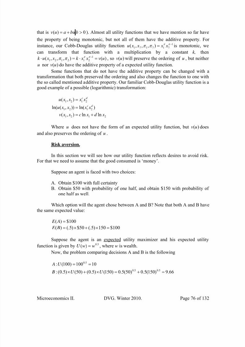
8/20/2019 ApuntesMicroeconomía II. David Vazquez.pdf
http://slidepdf.com/reader/full/apuntesmicroeconomia-ii-david-vazquezpdf 76/132
Microeconomics II. DVG. Winter 2010. Page 76 of 132
that is 0)( >+= bbuauv ). Almost all utility functions that we have mention so far have
the property of being monotonic, but not all of them have the additive property. For
instance, our Cobb-Douglas utility function 1
212121 ),,,( −= π π π π x x x xu is monotonic, we
can transform that function with a multiplication by a constant k, then
)(),,,(
1
212121 uv x xk x xuk =⋅=⋅ −π π
π π , so )(uv will preserve the ordering of u , but neitheru nor )(uv do have the additive property of a expected utility function.
Some functions that do not have the additive property can be changed with atransformation that both preserved the ordering and also changes the function to one withthe so called mentioned additive property. Our familiar Cobb-Douglas utility function is agood example of a possible (logarithmic) transformation:
2121
2121
2121
lnln),(
)ln()),(ln(
),(
xd xc x xv
x x x xu
x x x xu
d c
d c
+=
=
=
Where u does not have the form of an expected utility function, but )(uv does
and also preserves the ordering of u .
Risk aversion.
In this section we will see how our utility function reflects desires to avoid risk.For that we need to assume that the good consumed is ‘money’.
Suppose an agent is faced with two choices:
A. Obtain $100 with full certaintyB. Obtain $50 with probability of one half, and obtain $150 with probability of
one half as well.
Which option will the agent chose between A and B? Note that both A and B havethe same expected value:
100$)( = A E
100$150)5(.50$)5(.)( =×+×= B E
Suppose the agent is an expected utility maximizer and his expected utility
function is given by 5.0)( wwU = , where w is wealth.
Now, the problem comparing decisions A and B is the following
66.9)150(5.0)50(5.0)150()5.0()50()5.0(:
10100)100(:
5.05.0
5.0
=+=×+×
==
U U B
U A

8/20/2019 ApuntesMicroeconomía II. David Vazquez.pdf
http://slidepdf.com/reader/full/apuntesmicroeconomia-ii-david-vazquezpdf 77/132
Microeconomics II. DVG. Winter 2010. Page 77 of 132
In this case, )()( A E B E < , so agent chooses A rather than B, because the
expected utility is greater in that case, this is an example of a ‘risk averse’ agent. Let’sdefine what is risk aversion.
Definition: Let G be a gamble, the agent is said to be risk averse if
( ) ( ))()( GU E G E U > , where ( ))(G E U is the utility of the expected value of the gamble,and ( ))(GU E is the expected value of the utility of the gamble. This means that the agent
prefers to have the expected value of his wealth ( ))(G E U rather than to face the gamble
( ))(GU E .
Risk Aversion
w0
E(U(G))=U(w’)
E(G)
Utility
w1 w2
U(w)
u(w)E(G)-w’
w’
Numerical example:
Suppose the agent has an expected utility function given by 5.0)( wwU = , where w
is wealth, and G=[$50 with probability one half, $150 with probability one half].
( ) 10100)100())150(5.)50(5(.)( 5.0 ===+= U U G E U
( ) 66.9)150(5.)50(5.)150(5.)50(5.)( 5.05.0 =+=+= U U GU E
Now, comparing, we have that ( ) ( ))()( GU E G E U > , so the agent is risk averse.

8/20/2019 ApuntesMicroeconomía II. David Vazquez.pdf
http://slidepdf.com/reader/full/apuntesmicroeconomia-ii-david-vazquezpdf 78/132

8/20/2019 ApuntesMicroeconomía II. David Vazquez.pdf
http://slidepdf.com/reader/full/apuntesmicroeconomia-ii-david-vazquezpdf 79/132
Microeconomics II. DVG. Winter 2010. Page 79 of 132
Risk lover
w0
E(U(G))
E(G)
Utility
w1 w2
U(w)
u(w)
Definition: Let G be a gamble, the agent is said to be risk neutral if( ) ( ))()( GU E G E U = , where ( ))(G E U is the utility of the expected value of the gamble,
and ( ))(GU E is the expected utility of the gamble. The correspondent graph is a straight
line from the origin (neither concave nor convex).
Numerical example:
Suppose the agent has an expected utility function given by 5.0)( wwU = , where w
is wealth, and G=[$4 with probability one half, $16 with probability one half].
( ) 16.310)10())16(5.)4(5(.)(
5.0
===+= U U G E U ( ) 3)16(5.)4(5.)16(5.)4(5.)( 5.05.0 =+=+= U U GU E
Now, comparing, we have that ( ) ( ))()( GU E G E U > , so the agent is risk averse.

8/20/2019 ApuntesMicroeconomía II. David Vazquez.pdf
http://slidepdf.com/reader/full/apuntesmicroeconomia-ii-david-vazquezpdf 80/132
Microeconomics II. DVG. Winter 2010. Page 80 of 132
Graphical example of risk (2)
w0
E(U(G))=3
10=E(G)
Utility
4 16
U(10)=3.16
u(w)=w1/2
w’
U(16)=4
U(4)= 2
Definition: The certainty equivalent of a gamble G is a level of wealth w’ suchthat ( ) ( ))(' GU E wU = .
Expected utility can be defined in the following way: Let define a game
2211 ,;, w pw pG , where i p is the probability of obtaining certain level of wealth iw .
( ) 2211 w pw pG E +=
( ) )()()( 2211 wU pwU pGU E += , this is the expected utility.
Remark:
Because almost all people have a diminishing marginal utility of income, peopleare in fact risk averse. The opposite case would be a ‘greedy’ person (a risk loving person).

8/20/2019 ApuntesMicroeconomía II. David Vazquez.pdf
http://slidepdf.com/reader/full/apuntesmicroeconomia-ii-david-vazquezpdf 81/132
Microeconomics II. DVG. Winter 2010. Page 81 of 132
LESSON 12: Revealed Preference.
Observable preferences.
There is an issue about the act of choice that bases their behavior on ranking preferences. Preferences can be mapped through utility functions. Utility is a unit ofvalue that is related with consumer’s satisfaction, but is not observable. We can notobserve utility, but we might observe consumer’s behavior. Therefore, we can inferagent’s preferences given their observable behavior. This is a reasonable way to look at behavior in the short run, just assuming that people do not change their preferences veryoften.
Let’s see how this work. Given two different bundles of goods ),( 21 x x and
),( 21 y y , if we assume that preferences are (strictly) convex,9 that will give us a unique
optimal bundle of goods chosen on each consumer’s budget, either ),( 21 x x or ),( 21 y y ,
but not both.
In the diagram below, if it happens that bundle ),( 21 x x is chosen rather than
),( 21 y y , we observe that both bundles are attainable by the consumer’s budget, then we
infer that ),( 21 x x is better for the consumer than ),( 21 y y . Bundle ),( 21 y y ‘could’ be
chosen, but it wasn’t.
Is clear that all bundles below the budget line are revealed worse to bundle
),( 21 x x (remember strict convexity). Assuming given prices, it must be happening the
following equivalences:
9 A non convex set might violate this assumption, an example can be plotted.

8/20/2019 ApuntesMicroeconomía II. David Vazquez.pdf
http://slidepdf.com/reader/full/apuntesmicroeconomia-ii-david-vazquezpdf 82/132
Microeconomics II. DVG. Winter 2010. Page 82 of 132
m x p x p =+ 2211
Because we assume the subject is indeed optimizing, that is the reason he choosesthis bundle, and
m y p y p ≤+ 2211
Because the rest of the bundles are affordable. Now putting together the lastequations, we have that
22112211 y p y p x p x p +≥+
That is the same to say that ),( 21 x x is directly revealed preferred to ),( 21 y y ,
whenever ),(),( 2121 x x y y ≠ . This is not the same to say that ),( 21 x x is preferred to
),( 21 y y , we just say that ),( 21 x x was chosen when ),( 21 y y was affordable.Being more formal, the principle of revealed preference stated that when we
have two bundles of goods ),( 21 x x , ),( 21 y y , and the one chosen is ),( 21 x x , holding the
weak inequality 22112211 y p y p x p x p +≥+ and maximizing behavior, we can say indeed
that ),(),( 2121 y y x x f , where the relation f holds for revealed preference.
An indirect application of this principle comes from the introduction of a third
bundle of goods ),( 21 z z , and another set of prices ),( 21 qq described with a different
(sloped) budget line. If we say that 22112211 zq zq yq yq +≥+ , we know by the principle of
revealed preference that ),(),( 2121 z z y y f . Assuming nice preference behavior, that is,
transitivity, if we have ),(),( 2121 y y x x f and ),(),( 2121 z z y y f , we know for sure that
),(),( 2121 z z x x f , this is the same to say that ),( 21 x x is indirectly revealed to ),( 21 z z .
We show this on the diagram below:
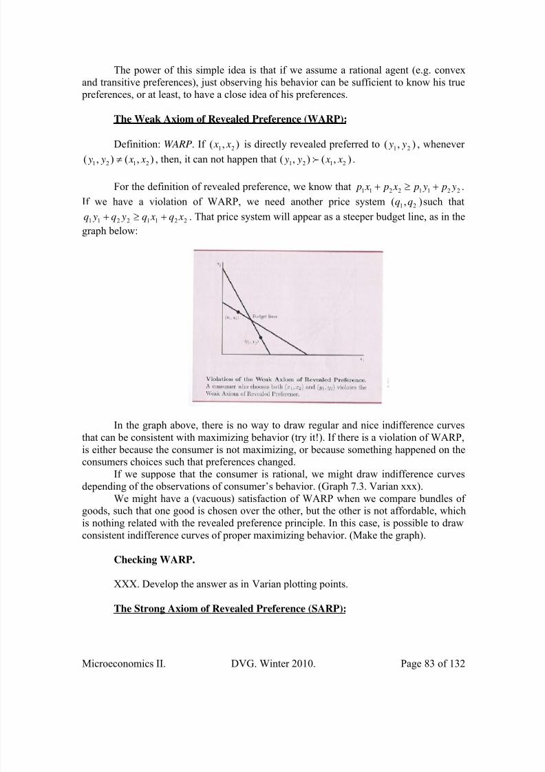
8/20/2019 ApuntesMicroeconomía II. David Vazquez.pdf
http://slidepdf.com/reader/full/apuntesmicroeconomia-ii-david-vazquezpdf 83/132
Microeconomics II. DVG. Winter 2010. Page 83 of 132
The power of this simple idea is that if we assume a rational agent (e.g. convexand transitive preferences), just observing his behavior can be sufficient to know his true preferences, or at least, to have a close idea of his preferences.
The Weak Axiom of Revealed Preference (WARP):
Definition: WARP. If ),( 21 x x is directly revealed preferred to ),( 21 y y , whenever
),(),( 2121 x x y y ≠ , then, it can not happen that ),(),( 2121 x x y y f .
For the definition of revealed preference, we know that 22112211 y p y p x p x p +≥+ .
If we have a violation of WARP, we need another price system ),( 21 qq such that
22112211 xq xq yq yq +≥+ . That price system will appear as a steeper budget line, as in the
graph below:
In the graph above, there is no way to draw regular and nice indifference curvesthat can be consistent with maximizing behavior (try it!). If there is a violation of WARP,is either because the consumer is not maximizing, or because something happened on theconsumers choices such that preferences changed.
If we suppose that the consumer is rational, we might draw indifference curvesdepending of the observations of consumer’s behavior. (Graph 7.3. Varian xxx).
We might have a (vacuous) satisfaction of WARP when we compare bundles ofgoods, such that one good is chosen over the other, but the other is not affordable, whichis nothing related with the revealed preference principle. In this case, is possible to drawconsistent indifference curves of proper maximizing behavior. (Make the graph).
Checking WARP.
XXX. Develop the answer as in Varian plotting points.
The Strong Axiom of Revealed Preference (SARP):

8/20/2019 ApuntesMicroeconomía II. David Vazquez.pdf
http://slidepdf.com/reader/full/apuntesmicroeconomia-ii-david-vazquezpdf 84/132
Microeconomics II. DVG. Winter 2010. Page 84 of 132
The definition of SARP, comes naturally from the definition of indirect revealed preference:
Definition: SARP. If ),( 21 x x is directly revealed preferred to ),( 21 y y , by direct or
indirect means, whenever ),(),( 2121 x x y y ≠ , then, it can not happen that ),(),( 2121 x x y y f
by direct or indirect revealed preference.
This is a natural complement of WARP, but stronger in the sense that it does onlyrequires optimizing behavior, but transitive preferences as well, so we can infer that bundles satisfying SARP comes from a well behave and nice indifference curves, so“SARP is both a necessary and a sufficient condition for observed choices to becompatible with the economic model of consumer choice” (Varian, 2003, p. 129). SARPgive us all the restrictions that we have in an optimizing model, because if consumer’s behavior is consistent with SARP, we can find indifference curves that approximate such behavior. This approximation can be done using econometric tools.
10 The corollary for
this theory is that it connects nicely consumer theory with real life, observed behavior
with consumer’s preferences..
10 For instance, considering that a utility function has the following shaped c x x x xU 2121 ),( = , a
logarithmic transformation will looks like 2121 loglog),( xd xc x xV += , which can be approximated,
with enough data, in a econometric model like ε β β α +++= 2211 x x y (check subscripts xxx).
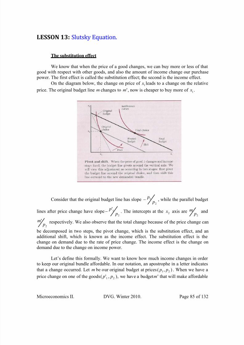
8/20/2019 ApuntesMicroeconomía II. David Vazquez.pdf
http://slidepdf.com/reader/full/apuntesmicroeconomia-ii-david-vazquezpdf 85/132
Microeconomics II. DVG. Winter 2010. Page 85 of 132
LESSON 13: Slutsky Equation.
The substitution effect
We know that when the price of a good changes, we can buy more or less of thatgood with respect with other goods, and also the amount of income change our purchase power. The first effect is called the substitution effect; the second is the income effect.
On the diagram below, the change on price of 1 x leads to a change on the relative
price. The original budget line m changes to 'm , now is cheaper to buy more of 1 x .
Consider that the original budget line has slope2
1
p p− , while the parallel budget
lines after price change have slope2
1' p
p− . The intercepts at the 2 x axis are2 p
m and
2
' p
m respectively. We also observe that the total change because of the price change can
be decomposed in two steps, the pivot change, which is the substitution effect, and anadditional shift, which is known as the income effect. The substitution effect is the
change on demand due to the rate of price change. The income effect is the change ondemand due to the change on income power.
Let’s define this formally. We want to know how much income changes in orderto keep our original bundle affordable. In our notation, an apostrophe in a letter indicates
that a change occurred. Let m be our original budget at prices ),( 21 p p . When we have a
price change on one of the goods ),'( 21 p p , we have a budget 'm that will make affordable
8/20/2019 ApuntesMicroeconomía II. David Vazquez.pdf
http://slidepdf.com/reader/full/apuntesmicroeconomia-ii-david-vazquezpdf 86/132
Microeconomics II. DVG. Winter 2010. Page 86 of 132
the old consumption bundle. Since both m and 'm can afford the same consumption
bundle ),( 21 x x , we have that
2211 x p x pm += and 2211'' x p x pm +=
Subtracting these equations, we have that
]'[
)'('
111
22112211
p p x
x p x p x p x pmm
−=
+−+=−
If we define mΔ as the change on income 'mm − , and we similarly do this for
prices, we can rewrite our last identity as follows
][ 11 p xm Δ=Δ
An implication of this is that a change on price is directly related with a change onincome. We remember that the substitution effect is the change on demand for one good
when its price changes to ),'( 21 p p , then also income changes to 'm , then
),()','( 11111 m p xm p x x s −=Δ
This is our substitution effect.
The income effect.
For another change on demand due to a price change, let’s observe the shift of our budget line in the diagram above. What is seen as the parallel line above the pivoted budget line, that is the change on income keeping prices constant, this is the incomeeffect.
Being more precise, our income effect is the change on demand n x1Δ of good one
due to the change on income from m to 'm keeping prices constant,
)','(),'( 11111 m p xm p x xn −=Δ
Income effect can be positive or negative. It is straightforward to see that whenhave more disposable income, we might tend to increase our consumption of that good, if
that good is a normal good. The opposite happens when we consider an inferior good, aswe increase our income we might want to consume other kind of goods rather than thegood itself, then, the income effect in this case is negative.
The Slutsky equation.
8/20/2019 ApuntesMicroeconomía II. David Vazquez.pdf
http://slidepdf.com/reader/full/apuntesmicroeconomia-ii-david-vazquezpdf 87/132
Microeconomics II. DVG. Winter 2010. Page 87 of 132
A total change in demand 1 xΔ is the change in demand of the good when we
change the price of it, ceteris paribus (holding income and the price of the other goodsconstant), that is
),(),'( 11111 m p xm p x x −=Δ
We also know that total change in demand 1 xΔ can be decomposed in
substitution and income effect, so
ns x x x 111 Δ+Δ=Δ
Plugging the income and substitution effects equations on the previous one, wehave that
( ) ( ))','(),'(),()','(),(),'( 111111111111
111
m p xm p xm p xm p xm p xm p x
x x x ns
−+−=−
Δ+Δ=Δ
This is the Slutsky decomposition; it expresses mathematically the total change ondemand on income and substitution effects separately.
Usually, the Slutsky decomposition is expressed in terms of rates of price change.First we define the negative impact of income effect as follows,
nm xm p xm p x x 111111 ),'()','( Δ−=−=Δ
So
ms x x x 111 Δ−Δ=Δ
Dividing everything over 1 pΔ , and considering that1
111 ][ x
m p p xm
Δ=Δ⇒Δ=Δ ,
we can rewrite the Slutsky decomposition in the following way
11
1
1
1
1
1
1
1
1
1
1 x
m
x
p
x
p
x
p
x
p
x
p
x msms
Δ
Δ−
Δ
Δ=
Δ
Δ⇒
Δ
Δ−
Δ
Δ=
Δ
Δ
This is the so called Slutsky equation, which is the decomposed change ondemand when price changes and normalized by the price change.
Some useful identities that come from the previous equations:
Using ),(),'( 11111 m p xm p x x −=Δ and dividing over 1 pΔ , we have that

8/20/2019 ApuntesMicroeconomía II. David Vazquez.pdf
http://slidepdf.com/reader/full/apuntesmicroeconomia-ii-david-vazquezpdf 88/132
Microeconomics II. DVG. Winter 2010. Page 88 of 132
1
1111
1
1 ),(),'(
p
m p xm p x
p
x
Δ
−=
Δ
Δ,
This is the rate of change of demand when price changes, holding income
constant.
Using ),()','( 11111 m p xm p x x s −=Δ , and dividing over 1 pΔ , we have that
1
1111
1
1 ),()','(
p
m p xm p x
p
x s
Δ
−=
Δ
Δ
This is the rate of change on demand when price changes, adjusting income insuch way that we can keep buying the original bundle, this is the substitution effect.
Using nm xm p xm p x x 111111 ),'()','( Δ−=−=Δ , dividing over mΔ ,
11111
11
11111
),'()','(
),'()','(
xm
m p xm p x x
m
x
m
m p xm p x
m
x
m
m
⋅Δ
−=⋅
Δ
Δ
Δ
−=
Δ
Δ
and considering that1
111 ][ x
m p p xm
Δ=Δ⇒Δ=Δ , we have that
111111
1
11111
1
1
11111
11
),'()','(
),'()','(1
),'()','(
p xm
m p xm p x x
xm
m p xm p x
p
x
xm
m p xm p x xm
x
m
m
m
Δ⋅Δ
−=Δ
⋅Δ
−=
Δ⋅
Δ
⋅Δ
−=⋅ΔΔ
Recall that 11 p x Δ is the change on income in order to keep the old bundle
feasible.11
Homework. Calculating substitution and income effect as the example in Varian
p. 140.
(xxx) Maybe elaborate more on inferior goods.
11 Note that ),'()','(),'()','(
1111111111
1 m p xm p x p xm
m p xm p x xm −=Δ⋅
Δ
−=Δ , which is our old
friend back.

8/20/2019 ApuntesMicroeconomía II. David Vazquez.pdf
http://slidepdf.com/reader/full/apuntesmicroeconomia-ii-david-vazquezpdf 89/132
Microeconomics II. DVG. Winter 2010. Page 89 of 132
LESSON 14: General Equilibrium.
What is General Equilibrium?
When we study market behavior in a single particular market, considering thesupply and the demand side, that is a partial equilibrium analysis. Sometimes thisanalysis needs to be carried out further with more than one market, this is the generalequilibrium framework; how the demand and the supply sides interact in more than onemarket. It is true that in partial equilibrium analysis, prices vary in regards to theinteraction among producers and consumers, doing this consideration in the generalequilibrium framework is possible but difficult, so is normal to look first at generalequilibrium analysis in the competitive market structure, that is the reason we take pricesas given in the following notes. For the sake of simplicity, we start our analysis with asfewer elements as possible, which means two goods and two consumers.
The Edgeworth Box
We already said that for the sake of simplicity, only two goods and twoconsumers were included in our analysis. An additional restriction of no producers, and because of that no production, is made when we say that there are fixed endowments inour economy. That is the reason the simplest form of general equilibrium analysis ismade in a pure exchange economy. A particular tool that has been used widely forindividual’s exchange in the market is the Edgeworth Box, which portrays twoconsumers, one in the traditional fashion (Consumer A below), with the origin on thelower left corner, with indifference curves that increase their utility to the upper and right
direction. Another consumer is shown in a diagram that rotates 180o
, (see belowConsumer B’s side). Is clear that for consumer B, the origin is in the upper right corner,and his utilities increase to the lower and left direction.
Consumer A’s side
Good 1
M
1 A
x 1 Aω
2
A x
2
Aω
),(21
A A A x xU
Good 2
W
A0
Consumer B’s side
Good 1
M
Good 2 ),( 21
B B B x xU
W
1 B x 1
Bω
2
B x
2
Bω
B0
Both consumers together have a mutually exclusive share of goods, and for ouranalysis, there is no other good outside the economy rather than inside the box. It isconvenient to say that the initial endowment is W (shown below), but there might be

8/20/2019 ApuntesMicroeconomía II. David Vazquez.pdf
http://slidepdf.com/reader/full/apuntesmicroeconomia-ii-david-vazquezpdf 90/132
Microeconomics II. DVG. Winter 2010. Page 90 of 132
exchange among the consumers in order to attain highest indifference curves on theirown side, as it can be allocation M on the same diagram.
The Edgeworth Box
Good 1
M
1 A x 1
Aω
2
A x
2
Aω
),(21
A A A x xU
Good 2 ),( 21
B B B x xU
W
1 B x 1
Bω
2
B x
2
Bω
)( 11 B A x x + A0
B0)( 22
B A x x +
It is clear that the total quantity of the final allocation of goods M is equal to thetotal quantity of the initial endowment W, that is
1111
B A B A x x ω ω +=+
2222 B A B A x x ω ω +=+
This means that there are no transaction costs and no waste on this economy.
Pure Exchange Economy
We already said that for the sake of simplicity, only two goods and twoconsumers were included in our analysis. An additional restriction of no producers, and because of that, no production, is made when we say that there are fixed endowments inour economy. That is the reason the simplest form of general equilibrium analysis ismade in a pure exchange economy.
So, in in this course we consider a pure exchange economy with two consumers(A and B), two goods (1 and 2), no producers and no production (only allocation of initialendowment). Endowments are considered as follows
Consumer 1, 21 , A A A ω ω ω =
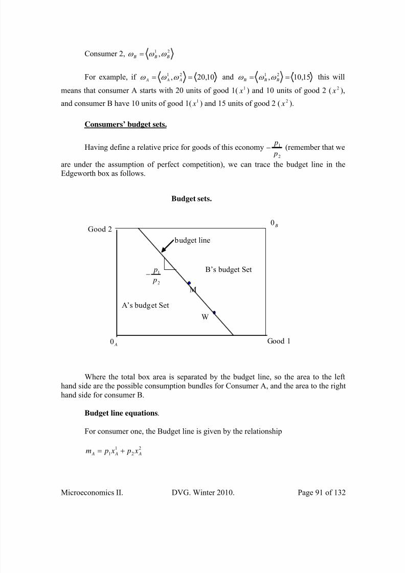
8/20/2019 ApuntesMicroeconomía II. David Vazquez.pdf
http://slidepdf.com/reader/full/apuntesmicroeconomia-ii-david-vazquezpdf 91/132
Microeconomics II. DVG. Winter 2010. Page 91 of 132
Consumer 2, 21 , B B B ω ω ω =
For example, if 10,20, 21 == A A A ω ω ω and 15,10, 21 == B B B ω ω ω this will
means that consumer A starts with 20 units of good 1( 1 x ) and 10 units of good 2 ( 2
x ),
and consumer B have 10 units of good 1( 1 x ) and 15 units of good 2 ( 2 x ).
Consumers’ budget sets.
Having define a relative price for goods of this economy2
1
p
p− (remember that we
are under the assumption of perfect competition), we can trace the budget line in theEdgeworth box as follows.
budget line
Budget sets.
Good 1
M
Good 2
W
A0
B0
A’s budget Set
B’s budget Set
2
1
p
p−
Where the total box area is separated by the budget line, so the area to the lefthand side are the possible consumption bundles for Consumer A, and the area to the righthand side for consumer B.
Budget line equations.
For consumer one, the Budget line is given by the relationship
2
2
1
1 A A A x p x pm +=

8/20/2019 ApuntesMicroeconomía II. David Vazquez.pdf
http://slidepdf.com/reader/full/apuntesmicroeconomia-ii-david-vazquezpdf 92/132
Microeconomics II. DVG. Winter 2010. Page 92 of 132
Of course, the budget constraint will satisfy the initial endowment for consumerone, that is
2
2
1
1 A A A p pm ω ω +=
In general equilibrium, income is equal to the value of the initial endowment.Consequently, the consumer two will satisfy the following conditions
2
2
1
1 B B B x p x pm +=
and
2
2
1
1 B B B p pm ω ω += ,
General competitive equilibrium.
Definition. In a two-good, two-consumer economy, a general competitive
equilibrium of pure exchange (no production considered) is a pair of prices 21, p p and a
quadruple set of quantities 2121 ,,, B B A A x x x x such that:
1. Both consumers are maximizing their utility subject to the budgetconstraint.
2. Market clearance condition: demand is equal to supply, that is11111 ω ω ω =+=+ B A B A x x and 22222 ω ω ω =+=+ B A B A x x (Aggregate
consumer demand is 11
B A x x + and 22
B A x x + , so aggregate supply is 1ω and
2ω ).

8/20/2019 ApuntesMicroeconomía II. David Vazquez.pdf
http://slidepdf.com/reader/full/apuntesmicroeconomia-ii-david-vazquezpdf 93/132
Microeconomics II. DVG. Winter 2010. Page 93 of 132
General competitive equilibrium
Good 1
M
Good 2
W
A0
B0
Competitiveequilibrium
allocation
2
1
p p−
1 A x 1
Aω
2
A x
2 Aω
1 B x 1
Bω
2
B x
2 Bω
Disequilibrium.
Lets examine the first case, both consumers are satisfying maximizing behavior, but market clearance condition do not hold.
Disequilibrium
Good 1
M’
Good 2
W
A0
B0
Market
clearance fails
1 A x 1
Aω
2 A x
2 Aω
1 B x 1
Bω
2 B x2
Bω
M’’
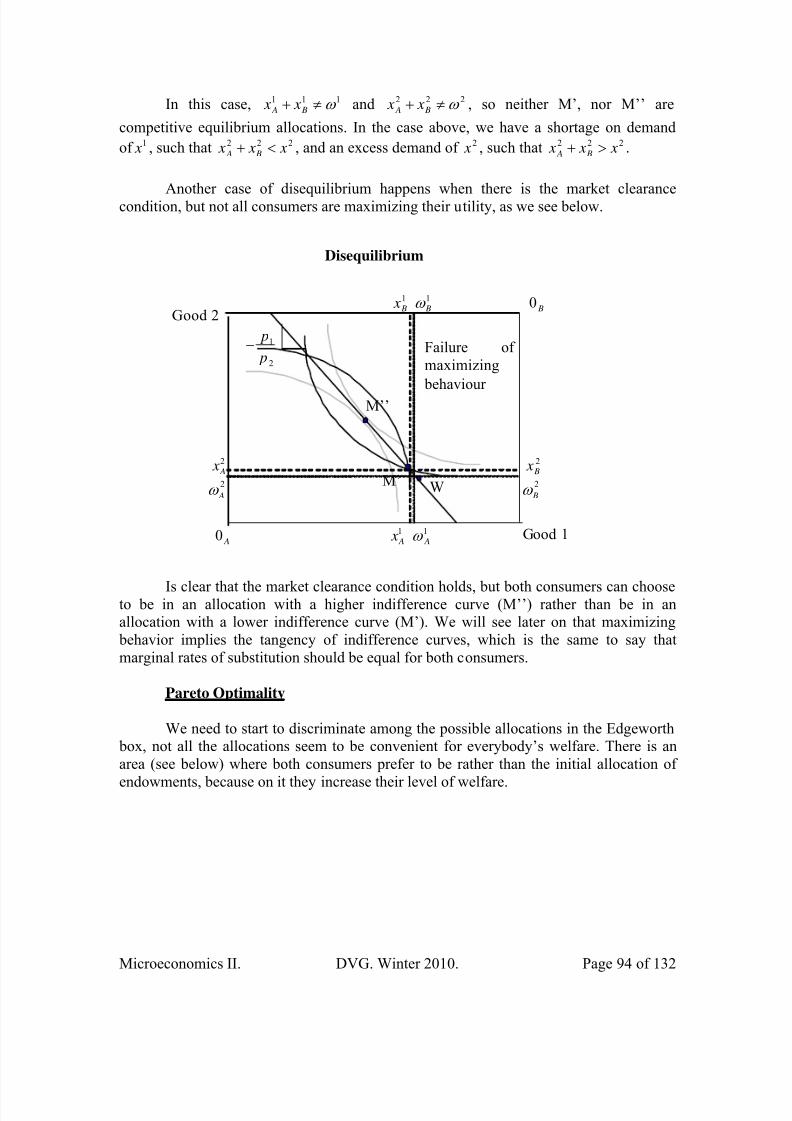
8/20/2019 ApuntesMicroeconomía II. David Vazquez.pdf
http://slidepdf.com/reader/full/apuntesmicroeconomia-ii-david-vazquezpdf 94/132
Microeconomics II. DVG. Winter 2010. Page 94 of 132
In this case, 111 ω ≠+ B A x x and 222 ω ≠+ B A x x , so neither M’, nor M’’ are
competitive equilibrium allocations. In the case above, we have a shortage on demand
of 1 x , such that 222 x x x B A <+ , and an excess demand of 2 x , such that 222 x x x B A >+ .
Another case of disequilibrium happens when there is the market clearancecondition, but not all consumers are maximizing their utility, as we see below.
Disequilibrium
Good 1
Good 2
W
A0
B0
Failure ofmaximizing
behaviour
2
1
p
p−
1 A x 1
Aω
2 A x2
Aω
1 B x 1
Bω
2 B x2
Bω M’
M’’
Is clear that the market clearance condition holds, but both consumers can chooseto be in an allocation with a higher indifference curve (M’’) rather than be in anallocation with a lower indifference curve (M’). We will see later on that maximizing behavior implies the tangency of indifference curves, which is the same to say thatmarginal rates of substitution should be equal for both consumers.
Pareto Optimality
We need to start to discriminate among the possible allocations in the Edgeworth box, not all the allocations seem to be convenient for everybody’s welfare. There is anarea (see below) where both consumers prefer to be rather than the initial allocation of
endowments, because on it they increase their level of welfare.

8/20/2019 ApuntesMicroeconomía II. David Vazquez.pdf
http://slidepdf.com/reader/full/apuntesmicroeconomia-ii-david-vazquezpdf 95/132
Microeconomics II. DVG. Winter 2010. Page 95 of 132
Trade happens in shaded area
Good 1
M
1 A x 1
Aω
2
A x
2 Aω
Good 2
W
1 B x 1
Bω
2
B x
2 Bω
A0
B0
The idea of efficiency comes here, not all the points within this shade area are
preferred the same, that is the reason we go to the following topic.
Definition. A Pareto efficient allocation can be described as an allocation wherethere is no way to make a consumer better off without making worse off somebody else.There is no way to make both consumers better off neither (If there is time, work out themathematical conditions for Pareto allocations, as in Varian, Appendix p. 565).
Pareto Optimal Allocation
Good y
A0
B0
Pareto Optimal allocation
),( 22 y xU B
),(11
y xU A
8/20/2019 ApuntesMicroeconomía II. David Vazquez.pdf
http://slidepdf.com/reader/full/apuntesmicroeconomia-ii-david-vazquezpdf 96/132

8/20/2019 ApuntesMicroeconomía II. David Vazquez.pdf
http://slidepdf.com/reader/full/apuntesmicroeconomia-ii-david-vazquezpdf 97/132
Microeconomics II. DVG. Winter 2010. Page 97 of 132
Contract curve and initial endowment
Good x
Good y
W
A0
B0
Contract curve
212
212222 ),( y x y xU =
21
12
1
1111),( y x y xU =
0,1001 =ω
100,02 =ω
In the diagram, is clear that we need tangency among indifference curves in orderto have our contract curve, which is the same to say that slopes (marginal rates ofsubstitution) are equal. For consumer 1 we have that
1
1
21
12
1
1
21
12
1
1
11,1
11,1
11,,1
2
12
1
),(
),(),(
x
y
y x
y x
y x MU
y x MU y x MRS
y
x
y x
=
−
−=
=
−
−
Similarly, for consumer two happens that
2
222,,2 ),(
x y y x MRS y x =
We need both marginal rates of substitution be equal, then

8/20/2019 ApuntesMicroeconomía II. David Vazquez.pdf
http://slidepdf.com/reader/full/apuntesmicroeconomia-ii-david-vazquezpdf 98/132
Microeconomics II. DVG. Winter 2010. Page 98 of 132
2
2
1
1
22,,2
2
2
1
111,,1 ),(),(
x
y
x
y
y x MRS x
y
x
y y x MRS
y x y x
=
===
In order to express properly our contract curve, we need to separate 2 x from the
above equation, so
1
212
y
y x x = , (Equation 1)
This is the general relationship for the contract curve. In order to have a more precise idea of this contract curve, we need the market clearance condition(supply=demand), this is
1002121 ==+=+ x x x x x ω ω ω
and
1002121 ==+=+ y y y y y ω ω ω
we have that
10021 =+ x x (Equation 2)
21 100 x x −= (Equation 2’)
and
10021 =+ y y (Equation 3)
21 100 y y −= (Equation 3’)
Solving (1), (2’) and (3’), we plug them and we have that
22
222222
2222
2
2
2
2
2
22
2
100100
100100
)100()100(
100
)100(
100
)100(
y x
y x y y x x
x y y x
y
x
y
x
y
y x x
=
−=−
−=−
−
−=
−
−=

8/20/2019 ApuntesMicroeconomía II. David Vazquez.pdf
http://slidepdf.com/reader/full/apuntesmicroeconomia-ii-david-vazquezpdf 99/132
Microeconomics II. DVG. Winter 2010. Page 99 of 132
Then
22 y x = (Equation 4).
Which is our contract curve equation. We know for sure that consumers maximize
their utility in the set of allocations described by this relationship.
Now lets derive the general equilibrium allocation. For that, we need to find a pair
of prices y x p p , and a quadruple set of quantities 2211 ,,, y x y x such that both agents
maximize and markets clear.
For previous knowledge, we know that agents maximize (consumer 1) when
y
x
y
x y x
p
p
x
y
p
p y x MRS
=
=
1
1
11,,1 ),(
, (Equation 5, recall maximizing behavior.)
and
11
111
100 y p x p p
y p x pm
y x x
y x
+=
+= (Equation 6, this is the value of the initial allocation.)
For consumer two, and
y
x
y
x y x
p
p
x
y
p
p y x MRS
=
=
2
2
22,,2 ),(
(Equation 7)
And
22
222
100 y p x p p
y p x pm
y x y
y x
+=
+= (Equation 8)
Using (2), (3), (4), (5), (6) and (7), we have 6 equations and 6 unknowns, solvethe system.
Use (4) and (7),

8/20/2019 ApuntesMicroeconomía II. David Vazquez.pdf
http://slidepdf.com/reader/full/apuntesmicroeconomia-ii-david-vazquezpdf 100/132
Microeconomics II. DVG. Winter 2010. Page 100 of 132
12
2 == y
x
p
p
y
y (Equation 9)
Using (4), (8) and (9)
y
y
y y
y y y
p
p y
y p p
y p y p p
2
100
2100
100
2
2
22
=
=
+=
\Then
502 = y (Result 1).
So 502 = x (Result 2).
Using (5) and (9), we know that 11 y x = , and it will not be difficult to get that
501 = y (Result 3).
and 501 = x (Result 4).
So, the general equilibrium for this system is a pair of prices y x p p , such that
1= y
x
p
p (only relative prices matter, that is enough) and a quadruple set of quantities
50,50,50,50 such that both agents maximize and markets clear; the graph below
describes that. This allocation is also known as the competitive equilibrium allocation, orthe walrasian equilibrium.
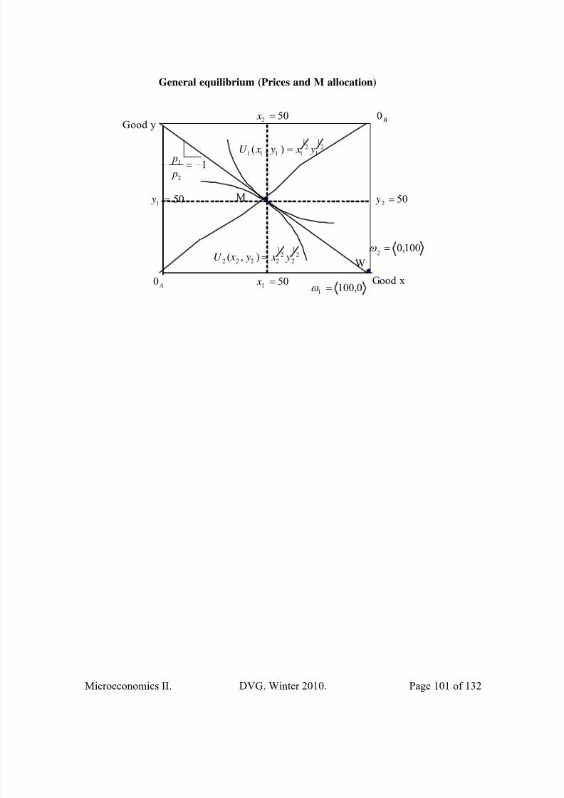
8/20/2019 ApuntesMicroeconomía II. David Vazquez.pdf
http://slidepdf.com/reader/full/apuntesmicroeconomia-ii-david-vazquezpdf 101/132

8/20/2019 ApuntesMicroeconomía II. David Vazquez.pdf
http://slidepdf.com/reader/full/apuntesmicroeconomia-ii-david-vazquezpdf 102/132
Microeconomics II. DVG. Winter 2010. Page 102 of 132
LESSON 15: Welfare theorems.
The contract curve.
Once that we know the definition of Pareto efficiency, all points that comply withthe P.O. criteria, where both agents are willing to trade such that no one is better offwithout hurting anybody else, those points can be depicted in our Edgeworth box as a linealong the box, which is known as the contract curve or the ‘Pareto set’. It will not bedifficult to show that this line is where the marginal rates of substitution are the same for both agents (proof in Varian, Appendix Ch. 30 p. 566).
Contract curve
Good y
A0
B0
Contract curve
),( 22 y xU B
),( 11 y xU A
The core.
We predict that consumers will trade and move away from the endowment W tosome bundle in the core (diagram below) because:
1. Both consumers are better off with some endowment in the core than atthe initial endowment W.
2. All bundles in the core are Pareto Optimal, hence all gains from trade have been exhausted.

8/20/2019 ApuntesMicroeconomía II. David Vazquez.pdf
http://slidepdf.com/reader/full/apuntesmicroeconomia-ii-david-vazquezpdf 103/132
Microeconomics II. DVG. Winter 2010. Page 103 of 132
Contract curve and the core
Good 1
M
Good 2
W
A0
B0
Contract curve
The core
In the diagram, we showed traditional indifference curves. In the case of convex(but not strictly convex) preferences, the core might be not only a smooth line, but an‘area’ where trade can occur.
First Welfare Theorem.
Once that we know how to achieve a competitive equilibrium (CE) in a tradeeconomy, we want to know if this allocation is the best option we can choose. We want
to know if all gains of trade are exhausted, otherwise, we could find another allocationwith no waste. The idea of efficiency is embedded in the Pareto Optimal (PO) criteria,nobody else can be better off without hurting anybody else.
If we want to see if a CE is PO, let’s check this by contradiction, which is the
usual way to know if this is happening. Considering that 2121 ,,, B B A A x x x x is the
competitive equilibrium allocation, now suppose this CE is not PO, therefore it should
exist another allocation 2121 ,,, B B A A y y y y such that
1111
B A B A y y ω ω +=+ (1)2222
B A B A
y y ω ω +=+ (2)
And
),(),( 2121 A A A A A x x y y f
),(),( 2121 B B B B B x x y y f
8/20/2019 ApuntesMicroeconomía II. David Vazquez.pdf
http://slidepdf.com/reader/full/apuntesmicroeconomia-ii-david-vazquezpdf 104/132
Microeconomics II. DVG. Winter 2010. Page 104 of 132
The first part says that this allocation is feasible, there is no excess nor shortagedemand of any good, the second part says that this allocation is preferred by bothconsumers to the CE allocation. Following this argument, if this newer allocation exists,it should cost more than the CE allocation, because both agents are maximizing utility,and if they are receiving more utility, logically they are spending more, that is
2
2
1
1
21
1
2
2
1
1 A A A A A A p p px x p y p y p ω ω +=+>+ 2
2
1
1
21
1
2
2
1
1 B B B B B B p p px x p y p y p ω ω +=+>+
Then
2
2
1
1
2
2
1
1 A A A A p p y p y p ω ω +>+ (3)2
2
1
1
2
2
1
1 B B B B p p y p y p ω ω +>+ (4)
If we put these two equations together, adding the left hand side of the first
equation, with the left hand side of the second equation, and similarly for the right handside, we have the following expression:
2
2
1
1
2
2
1
1
2
2
1
1
2
2
1
1 B B A A B B A A p p p p y p y p y p y p ω ω ω ω +++>+++ (5)
Which can be expressed like this:
)()()()( 22
2
11
1
22
2
11
1 B A B A B A B A p p y y p y y p ω ω ω ω +++>+++ (5’)
Putting together (1), (2) and (5’), we have that
)()()()( 222
111
222
111 B A B A B A B A y y p y y p y y p y y p +++>+++
This is clearly a contradiction, because an inequality can not hold if both sides arethe same. Also because the allocation chosen was arbitrary, this contradiction must holdfor any other allocation. Then, in any case that a CE is not PO can not be. It must be thecase that a Competitive Equilibrium is Pareto Optimal. •→ POCE , this result is known
as the First Theorem of Welfare Economics (further explanation in ‘The algebra ofefficiency’, page 555, Varian).
We just prove that under certain conditions, a competitive equilibrium is efficient.The issue about the ‘fairness’ of this allocation is not considered here, this just means thata CE will exhaust trade gains among traders. The issue of fairness might be clarified a bitwith our next topic. A corollary for these restrictions is such that this result holds whenthere is stability of prices (e.g. no inflation), we also need efficient allocation of resourcesat initial conditions.
In regards to the conditions just mentioned above, we observe that certaininstitutions (in the capitalist system) try to maintain such ‘stable’ conditions in order toguarantee an optimal result. For instance, the role of the central bank is price stability.
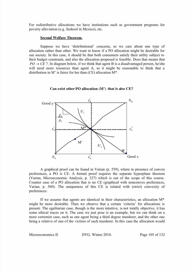
8/20/2019 ApuntesMicroeconomía II. David Vazquez.pdf
http://slidepdf.com/reader/full/apuntesmicroeconomia-ii-david-vazquezpdf 105/132

8/20/2019 ApuntesMicroeconomía II. David Vazquez.pdf
http://slidepdf.com/reader/full/apuntesmicroeconomia-ii-david-vazquezpdf 106/132
Microeconomics II. DVG. Winter 2010. Page 106 of 132
tend to be on one of the corners of the box, issue that would induce a very unequal result, but ethically chosen in the perspective of the researcher. So, the egalitarian criteria is onlyone possibility for fairness, there are others, like the needs based criteria (people withmore need deserve more), others that focus on performance (more efficients deservemore), others on opportunity (as long as the chances at the beginning are the same there
is fairness), and similar more.
Can exist other PO allocation (M’) that is also CE?
Good x
Original budget line
Good y
W
A0
B0
2U
2
1
p p−
1 A x
1
A x
1 B x
M* 2
A x
1U
M’
New budget line
In the diagram above, it is necessary a new budget set for both consumers, thoughthe relative price is the same. It can be also the case that a new CE, that is PO, can beachieved by a newer set of prices (not shown). But it can be said that indeed a ParetoOptimal allocation is a Competitive Equilibrium if preferences are convex CE PO → ,
this is the Second Theorem of Welfare Economics.The implication of the second theorem of welfare economics is such that it gives
space to an agency (say the government) in order to redistribute endowments such that a better allocation is achieved in society. It can also be the case that this newer allocation
can be achieved by a change on prices, issue that gives space for the government forintervention (make a diagram with post and pre equilibrium transfers; pre equilibriumtransfers are related with equality of opportunity). Transfers can be achieved with lump-sum taxes and subsidies, or progressive taxes as well (but there are some inefficiency onthis procedure).
This model of general equilibrium implies transaction costs equal to zero, but weknow that redistribution have positive transaction costs, that will give our model somesense of inefficiency. This is the main reason why neoclassical advocates support a lean

8/20/2019 ApuntesMicroeconomía II. David Vazquez.pdf
http://slidepdf.com/reader/full/apuntesmicroeconomia-ii-david-vazquezpdf 107/132
Microeconomics II. DVG. Winter 2010. Page 107 of 132
government. Another issue to say about transaction costs, is about ‘illegal’ transactioncosts, such that corruption, but there is no model that works well with corruption.Corruption is not a failure of the model, is a failure of human behavior regardless themodel.
It can be shown formally that a P.O. allocation will achieve the same conditions
of the C.E., that is a more formal way to prove the conditions for the second welfaretheorem (Varian, p. 565, Appendix).
Redistribution and traditional economics. (Vazquez-Guzman, 2008).
Traditional economics deals more with the issue of efficiency, rather than of theissue of inequality. Taking one of the most recurrent frameworks in this tradition, whichis the perfect competitive market, individual preferences and initial endowments aretaken as given. Achieved efficiency is good as long as the distribution is Pareto-efficient,where it is not possible to shift somebody’s welfare to a better condition withoutdecreasing the welfare position of somebody else. If there is some intervention for
redistribution, it should be done following the Kaldor-Hicks criterion, where the welfareof the society is raised if it is possible to change conditions such that the winners cancompensate fully the loss of the losers, and still gain. Following the utilitarianframework, the things that determine equilibrium are the individual rationality and theform of their utility preferences. Traditional economics steps aside from the definition ofsocial or distributive justice. A very standard quote in this sense claims: “Nothing wehave argued so far should lead us to believe that [Walrasian Equilibrium Allocations(WEA)] are necessarily “socially optimal” if we include in our notion of social optimalityany consideration for matters of “equity” or “justice” in distribution.” (Jehle and Reny,1998, p. 300). The coverage of this framework is bounded by ruling out the allocationsthat are not Pareto-efficient, which are not even likely to be candidates for being sociallyoptimal. Given some set of additional restrictions, a candidate for a socially justdistribution must be the set of the (existent) WEA.
One of the links provided as a mechanism to enhance a more equal social welfare,is the Second Welfare Theorem, which states that every Pareto-efficient allocation can besupported by a Competitive Equilibrium Allocation (figure below), but this frameworkhas some limitations. The redistribution of initial endowments from e to e*, should leadthis economy to achieve a socially superior competitive equilibrium allocation, which is _
x rather than ' x . Assuming zero transaction costs, if the society previously defined that _
x was a better result, the new redistribution allocation gives a chance for governmentintervention. This framework does not need a central planner in order to guarantee a
competitive equilibrium, but a third-party is still needed to reallocate the initialendowment.
12 Social Choice and Welfare theory faces other challenges (due mainly to
the puzzle represented by Arrow’s impossibility theorem), but definitely gives up thechoice of the best social state, and reassigns that responsibility to ethical grounds: “your
12 It is also possible to change this equilibrium with post-equilibrium transfers of income, or through someartificial change on prices (pre or post equilibrium) through subsidies or taxes (Adelman and Robinson,1989, p. 970).

8/20/2019 ApuntesMicroeconomía II. David Vazquez.pdf
http://slidepdf.com/reader/full/apuntesmicroeconomia-ii-david-vazquezpdf 108/132
Microeconomics II. DVG. Winter 2010. Page 108 of 132
choice of social welfare functions is a choice of distributional values and, therefore, achoice of ethical system” (Jehle and Reny, 1998, p. 356).
x1
O2x2
O1
-p*1 /p*2
e*
e
C
C
_
x
' x
Efficiency and social optimality in a two-person economy.
By the same token, it is said by Coleman that “The concept of ‘equality’ has no place in positive economic theory” (1987, p. 170). He explains that the very essence ofwhat he called ‘equality of result’ would imply a distribution process that would be theantithesis of the market. On the other side, normative economics tries to compensate for
the absence of the equality concept within the utilitarian welfaristic framework. Pigou(1938) came up with the, perhaps contestable, idea that because of the decreasingmarginal utility of money, the maximization of social welfare was inevitable, and indeed,that would lead to equality of incomes. That did not happen. This approach was rejected by Robbins (1938) with the critique of interpersonal comparisons of Jevons. As early asin 1897, Edgeworth pointed out before Robbins that equality of means would leadforcefully to an unequal distribution. Again, traditional economic theory does not fullycontain the important issue of inequality, so the theory still remains incomplete: “…, thevery programme of welfare economics –not to speak of the foundations for a policydesigned to bring equality – is emasculated” (Coleman, 1987, p. 170).
8/20/2019 ApuntesMicroeconomía II. David Vazquez.pdf
http://slidepdf.com/reader/full/apuntesmicroeconomia-ii-david-vazquezpdf 109/132

8/20/2019 ApuntesMicroeconomía II. David Vazquez.pdf
http://slidepdf.com/reader/full/apuntesmicroeconomia-ii-david-vazquezpdf 110/132
Microeconomics II. DVG. Winter 2010. Page 110 of 132
In order to show the criteria that divide our inequality measures, let’s mention asimple example. If we assume a given distribution, which is a set of numerical values(e.g. income) of n persons arranged in a vector form representing individual’s earnings,we can have the following distribution:
1,1,3 x =< > such that x denotes the income of a population of three individuals, because n=3,
where each of them 1 x , 2
x and 3 x earn or possess 1, 1 and 3 unit values respectively. On
the other hand, let’s define the distribution y in a similar way:1,2,2 y =< >
With a simple eye inspection, it is easy to see that the distribution y is moreegalitarian than distribution x, so we say that y is preferred to x. We might be applyingdirectly a measurement of inequality like the variance or the Gini coefficient; these kindof direct measures are, roughly speaking, a) ‘pragmatic’ inequality measures. On theother hand, if we want to consider the numerical values of the distribution as the seeds ofa social welfare utility function, we will be doing a b) ‘normative’ measurement, like the
Atkinson family of indices. Using a set of assumptions and properties, inequalitymeasurement can be done using c) ‘entropy’ measures, but that makes more sense to dowhen sub-groups within the distribution are considered.
In order to make a difference among different indices, we need to think on the d) properties of the inequality measures. Some people might argue that we are implicitlyconsidering some properties in the ranking of distributions x and y, as it is the non-transformation to the numerical values of income. If we use measures that applylogarithmic transformations to these incomes, it is conventionally agreed that we are stilltalking about pragmatic measures, like the standard deviation of logarithms, but it is truethat the ranking might be different using a transformation. On the other hand, in regardsof inequality measure properties, we might see a problem if we consider the following
distribution:1,2,"."w =< >
Where “.” represents a missing value in the survey data. We can think that eitherthe person, that was the subject of the interview, was not present at the moment of thesurvey, or his/her questionnaire was mishandled by the institution that makes the surveys.The ranking will be done depending on how the researcher treats that missing value.w can be considered sometimes as ' 1,2w =< > , such as the distribution has different
number of people than x or y, or it might be considered as '' 1,2,0w =< > , with different
mean income and with the same number of people as distribution x or y. Using the Ginicoefficient as an example, the ranking of x with w’ is different from the ranking of x with
w’’. So both the technical decisions and the properties used in the inequalitymeasurement do matter.
In the previous cases, both pragmatic and normative measures rely on theassumption of ‘completeness’ of the ranking distribution (Sen, 1973, pp. 5-9 & 47). Toconsider a counter example, let’s consider the following distribution
1,2,2,1,2,2 z =< >
For an inexpert reader, it might be sensible to compare distribution y withdistribution z. Indeed, a pragmatic measure like the Gini coefficient will give the same

8/20/2019 ApuntesMicroeconomía II. David Vazquez.pdf
http://slidepdf.com/reader/full/apuntesmicroeconomia-ii-david-vazquezpdf 111/132

8/20/2019 ApuntesMicroeconomía II. David Vazquez.pdf
http://slidepdf.com/reader/full/apuntesmicroeconomia-ii-david-vazquezpdf 112/132
8/20/2019 ApuntesMicroeconomía II. David Vazquez.pdf
http://slidepdf.com/reader/full/apuntesmicroeconomia-ii-david-vazquezpdf 113/132

8/20/2019 ApuntesMicroeconomía II. David Vazquez.pdf
http://slidepdf.com/reader/full/apuntesmicroeconomia-ii-david-vazquezpdf 114/132
Microeconomics II. DVG. Winter 2010. Page 114 of 132
(3) ∑=
≠⎥⎥⎦
⎤
⎢⎢⎣
⎡−⎟⎟
⎠
⎞⎜⎜⎝
⎛
−=
n
i
c
i
cGE c y
ccn y I
1
)( 1,0,1)1(
11)(
μ
(4)
∑=
===n
i iGE
c yn
y I L1
)0(0,log
1)(
μ
(5) ∑=
===n
i
ii
GE c y y
n y I T
1
)1( 1,log1
)(μ μ
where T is better known as the Theil measure, while L is the mean logarithmicdeviation, also known as a Theil’s ‘second’ measure (Shorrocks, 1980, p. 622; Sen, 1973, pp. 34; Foster and Sen, 1997, pp. 140 & 156). The definition of this family of indicesmakes it possible to include even Atkinson’s normative family of indices, as was pointedout by Shorrocks (1980, p. 622, n. 6). The re-expression of these measures considering
carefully the property of sub-group decomposability might be explored later.

8/20/2019 ApuntesMicroeconomía II. David Vazquez.pdf
http://slidepdf.com/reader/full/apuntesmicroeconomia-ii-david-vazquezpdf 115/132
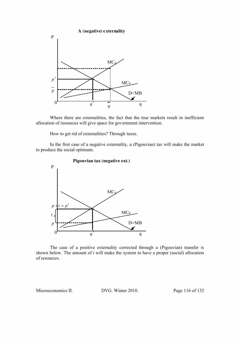
8/20/2019 ApuntesMicroeconomía II. David Vazquez.pdf
http://slidepdf.com/reader/full/apuntesmicroeconomia-ii-david-vazquezpdf 116/132
Microeconomics II. DVG. Winter 2010. Page 116 of 132
A (negative) externality
0
MCS
P
q
D=MB
q*q
* p
p
MCP
Where there are externalities, the fact that the true markets result in inefficientallocation of resources will give space for government intervention.
How to get rid of externalities? Through taxes.
In the first case of a negative externality, a (Pigouvian) tax will make the marketto produce the social optimum.
Pigouvian tax (negative ext.)
0
MCS
P
q
D=MB
*q
* pt p =+
p
MCP t
The case of a positive externality corrected through a (Pigouvian) transfer isshown below. The amount of t will make the system to have a proper (social) allocationof resources.
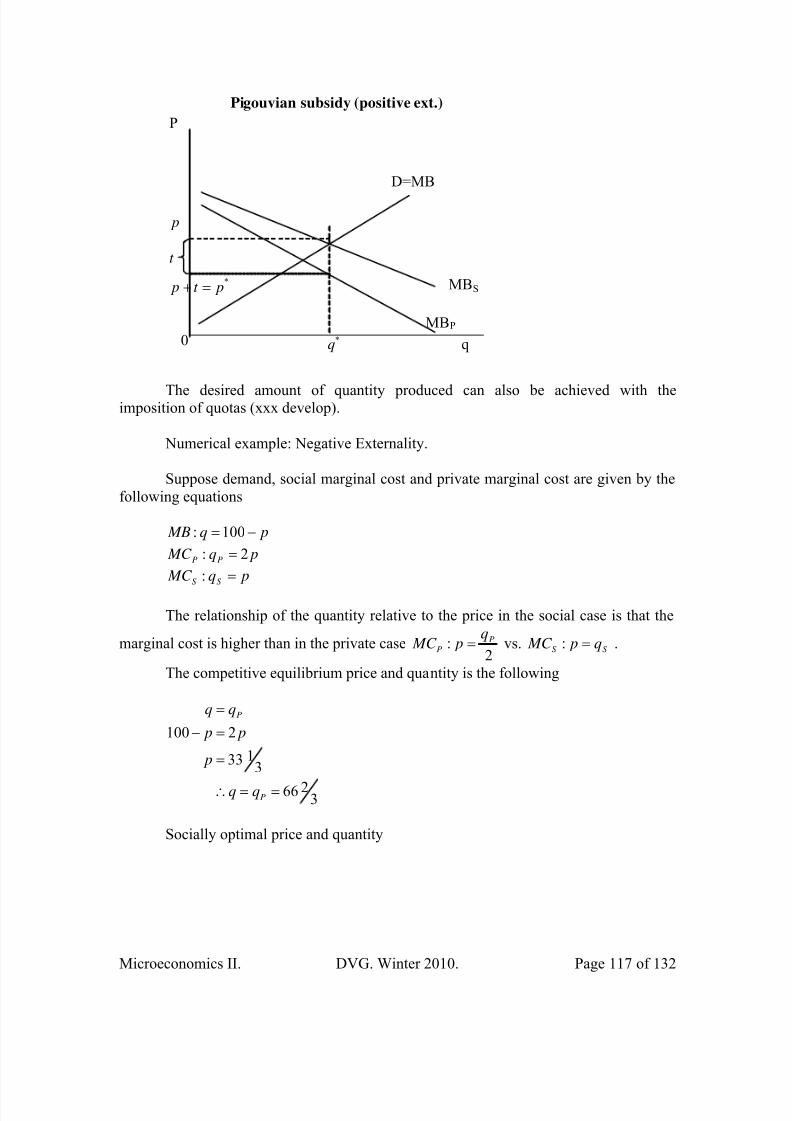
8/20/2019 ApuntesMicroeconomía II. David Vazquez.pdf
http://slidepdf.com/reader/full/apuntesmicroeconomia-ii-david-vazquezpdf 117/132

8/20/2019 ApuntesMicroeconomía II. David Vazquez.pdf
http://slidepdf.com/reader/full/apuntesmicroeconomia-ii-david-vazquezpdf 118/132
Microeconomics II. DVG. Winter 2010. Page 118 of 132
50
50
100
==∴
=
=−
=
P
S
p
p p
Tax that achieves the socially optimal quantity
Demand: )(10050 t p +−= (50 is taken from the above socially optimal quantity)
Supply: p250 = (we take the supply from the marginal social cost relationship in
order to know the price in the society).
25
2
50
=
= p
Once we know the price, we need to calculate the amount of tax.
25
2510050
)25(10050
=
−=+−
+−=
t
t
t
Check this on the private side.
50
)2550(2
2
=
−=
=
P
P
P
q
q
pq
Which is the predicted socially optimal quantity shall be produced.

8/20/2019 ApuntesMicroeconomía II. David Vazquez.pdf
http://slidepdf.com/reader/full/apuntesmicroeconomia-ii-david-vazquezpdf 119/132
Microeconomics II. DVG. Winter 2010. Page 119 of 132
LESSON 18: Public Goods.
The distinguishing feature of public goods, opposed to private goods, is that consumption
of a public good by one person does not necessarily preclude consumption of that good by another person. There are two characteristics that are usually associated to publicgoods, which are non-rivalry and non-exclusivity. Non-exclusive goods are those that provide benefits that no one can be excluded from consumption. Non-rival goods arethose that additional consumers may consume at zero marginal cost, for instance, anothercar in a bridge does not implies additional costs, the bridge is already there and no one isaffected if this car runs across the bridge. Conversely, private goods are exclusive andrival.
In some sense, a public good can be seen as a type of consumption externality,with the particular characteristic that public goods are consumed in equal shares byconsumers. If not all of them consume the same amount (e.g. security services by a police
department in case of theft), is assumed that all consumers have the same right to accessthose services; that is the reason the assumption of equal consumption of public goodsstill holds.
We care about public goods because, just like the other externalities, the freemarket fails to achieve an efficient allocation of resources when public goods are present.
Most of the times, we think that public goods are necessary, but we wonder whynot all the times that a public good is necessary then is provided. In other words, eventhough very often happens that the sum of the marginal benefits that a public good provides is less than the total cost of providing the good, in reality not all the publicgoods needed are provided. We need to think in what is meant for ‘free riding’.
A ‘free rider’ is a consumer of a (non-exclusive) good who does not pay for the
good consumed hoping that other consumers will. When other people, though they might be benefited from the provision of a public good, feel that others intend to ‘free-ride’, thewillingness to provide to such public goods diminish drastically.
In the diagram below a different marginal benefit from different consumers isshown. Considering that marginal cost is the same for both consumers (suppose prices ofraw material for the construction of a public facility are given), the first consumer have alower marginal benefit (e.g. think on the benefit for a childless couple in regards to a public park), the second consumer have a higher marginal benefit for this good (e.g. a
couple with children). The social efficient allocation would be ** ,q p but only
consumer 1 will buy that good, because as soon as ',' q p is chosen, because of the non-
exclusivity of the public good, consumer two will ‘free-ride’ and not buying butconsuming the good already provided.

8/20/2019 ApuntesMicroeconomía II. David Vazquez.pdf
http://slidepdf.com/reader/full/apuntesmicroeconomia-ii-david-vazquezpdf 120/132

8/20/2019 ApuntesMicroeconomía II. David Vazquez.pdf
http://slidepdf.com/reader/full/apuntesmicroeconomia-ii-david-vazquezpdf 121/132
Microeconomics II. DVG. Winter 2010. Page 121 of 132
one. As we construct the payoff matrix, we can see that there is an incentive to ‘free-ride’for both roommates, so the Nash equilibrium is the following
Public good free riding problem(Nash Equilibrium)
Buy2 Don't Buy2
Buy1 (-50,-50) (-50,100)
Don't Buy1 (100,-50) (0,0)
Roommate 2
Roommate 1
Then, no TV is bought.
Another way to get an insight about when to provide a public good is goingthrough the math in Varian pp. 644-647.
8/20/2019 ApuntesMicroeconomía II. David Vazquez.pdf
http://slidepdf.com/reader/full/apuntesmicroeconomia-ii-david-vazquezpdf 122/132
Microeconomics II. DVG. Winter 2010. Page 122 of 132
Bibliography.
Libro de Texto:
Varian, Hal R. Intermediate Microeconomics: A Modern Approach. Sixth Edition, Norton. (Para el mejor aprovechamiento del alumno, el libro de texto es obligatorioal empezar la tercer semana del curso).
Bibliografía complementaria y de apoyo:
• Varian, Hal R. Microeconomic Analysis.Third Edition, Norton.• Simon and Blume. Mathematics for Economists. Norton.
• Michael Parkin. Microeconomics. Sixth Edition (or higher). Addison Wesley.ISBN 0321112075.• Nicholson, Walter. Intermediate Microeconomics and its Application. NinthEdition. Thomson.

8/20/2019 ApuntesMicroeconomía II. David Vazquez.pdf
http://slidepdf.com/reader/full/apuntesmicroeconomia-ii-david-vazquezpdf 123/132

8/20/2019 ApuntesMicroeconomía II. David Vazquez.pdf
http://slidepdf.com/reader/full/apuntesmicroeconomia-ii-david-vazquezpdf 124/132

8/20/2019 ApuntesMicroeconomía II. David Vazquez.pdf
http://slidepdf.com/reader/full/apuntesmicroeconomia-ii-david-vazquezpdf 125/132

8/20/2019 ApuntesMicroeconomía II. David Vazquez.pdf
http://slidepdf.com/reader/full/apuntesmicroeconomia-ii-david-vazquezpdf 126/132

8/20/2019 ApuntesMicroeconomía II. David Vazquez.pdf
http://slidepdf.com/reader/full/apuntesmicroeconomia-ii-david-vazquezpdf 127/132
Microeconomics II. DVG. Winter 2010. Page 127 of 132
3. Competencia Imperfecta (Ch.27, Varian).
a. Oligopoliob. Duopolio (modelos de
Cournot y Stackelberg).
4. Teoría de juegos (Capítulos 28& 29, Varian).
a. Juegos de formaestratégica
i. Equilibrio deestrategiadominante
ii. Equilibrio deNash
iii. Ejemplos (Dilemade losprisioneros,Igualando lasmonedas, Labatalla de lossexos, Juego dela Gallina).
b. Juegos de formaextensiva
c. Conversión de juegos
de forma extensiva aestratégica (**)
Participación de la sesión8. Lectura previa delcapitulo 27, Varian.
Participación de la sesión9-10. Lectura previa de los
capítulos 28-29, Varian.
Sesión de preguntas. Participación en la sesiónde preguntas yrespuestas 11.
PRIMER EXAMEN PARCIAL Resolución de examenindividual en la sesión 12
Material de repaso primeraunidad.
Participación en la sesiónde énfasis 12’ al darle
solución al primer examenparcial.
Unidad 2Eleccion.(Sesiones 13-20)
5. Teoría del consumidor(Capítulos 2, 3, 4 & 5, Varian).
Participación de la sesión13-15. Lectura previa del
capítulos 2, 3, 4 y 5,Varian.
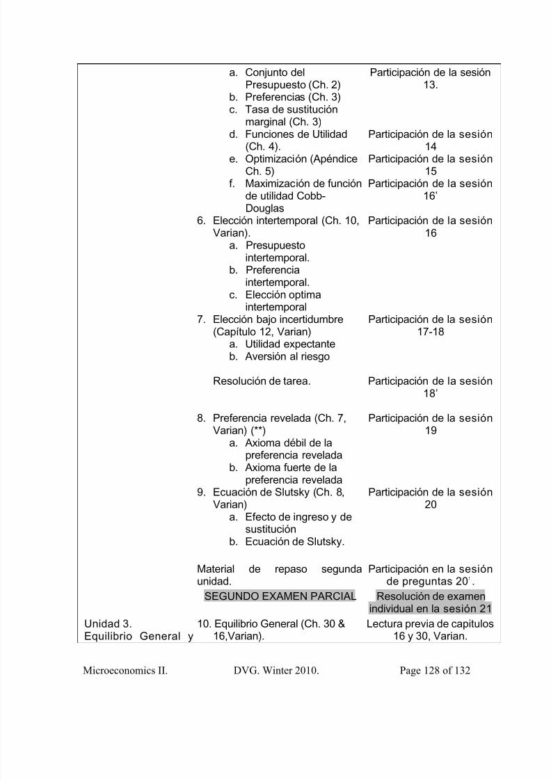
8/20/2019 ApuntesMicroeconomía II. David Vazquez.pdf
http://slidepdf.com/reader/full/apuntesmicroeconomia-ii-david-vazquezpdf 128/132
Microeconomics II. DVG. Winter 2010. Page 128 of 132
a. Conjunto delPresupuesto (Ch. 2)
b. Preferencias (Ch. 3)c. Tasa de sustitución
marginal (Ch. 3)
d. Funciones de Utilidad(Ch. 4).e. Optimización (Apéndice
Ch. 5)f. Maximización de función
de utilidad Cobb-Douglas
6. Elección intertemporal (Ch. 10,Varian).
a. Presupuestointertemporal.
b. Preferenciaintertemporal.c. Elección optima
intertemporal7. Elección bajo incertidumbre
(Capítulo 12, Varian)a. Utilidad expectanteb. Aversión al riesgo
Resolución de tarea.
8. Preferencia revelada (Ch. 7,Varian) (**)
a. Axioma débil de lapreferencia revelada
b. Axioma fuerte de lapreferencia revelada
9. Ecuación de Slutsky (Ch. 8,Varian)
a. Efecto de ingreso y desustitución
b. Ecuación de Slutsky.
Participación de la sesión13.
Participación de la sesión14
Participación de la sesión15
Participación de la sesión16’
Participación de la sesión16
Participación de la sesión17-18
Participación de la sesión18’
Participación de la sesión19
Participación de la sesión20
Material de repaso segundaunidad.
Participación en la sesiónde preguntas 20’.
SEGUNDO EXAMEN PARCIAL Resolución de examenindividual en la sesión 21
Unidad 3.Equilibrio General y
10. Equilibrio General (Ch. 30 &16,Varian).
Lectura previa de capitulos16 y 30, Varian.

8/20/2019 ApuntesMicroeconomía II. David Vazquez.pdf
http://slidepdf.com/reader/full/apuntesmicroeconomia-ii-david-vazquezpdf 129/132
Microeconomics II. DVG. Winter 2010. Page 129 of 132
Economía deldesarrollo. (Sesiones 22-30)
a. Caja de Edgeworth,preferencias ypresupuesto.
b. Equilibrio en la
economía deintercambio puro.c. Desequilibriod. Optimalidad de Paretoe. Algebra del Equilibrio
Generalf. Primer teorema de la
economía del desarrollog. Segundo teorema de la
economía del desarrolloh. Justicia, equidad y
distribución (Ch. 16, p.306, Varian) (**)11. Medición del bienestar (Lectura
provista por el instructor).a. Medición de la pobreza
y de la inequidad12. Fallos de mercado (Capítulo 33
&35, Varian).a. Externalidadesb. Bienes públicos.
Participación en la sesión22.
Participación de la sesión
23.
Participación en lassesión 24.
Participación de la sesión25.
Participación de la sesión26.
Participación de la sesión27-28
Participación de la sesión29-30
TERCER EXAMEN PARCIAL Resolución de examenindividual en la sesión 31
** Temas opcionales dependiendodel avance del curso.
VIII. Metodología y estrategias didácticas
1. Metodología Institucional:
a) Elaboración de ensayos, monografías e investigaciones (según el nivel) consultando fuentes
bibliográficas, hemerográficas, y "on line"
b) Elaboración de reportes de lectura de artículos actuales y relevantes a la materia en lengua inglesa
c)Se resolverán problemas teóricos y de aplicación.
2. Metodología y estrategias recomendadas para el curso:
A. Exposiciones: docente y alumno

8/20/2019 ApuntesMicroeconomía II. David Vazquez.pdf
http://slidepdf.com/reader/full/apuntesmicroeconomia-ii-david-vazquezpdf 130/132

8/20/2019 ApuntesMicroeconomía II. David Vazquez.pdf
http://slidepdf.com/reader/full/apuntesmicroeconomia-ii-david-vazquezpdf 131/132

8/20/2019 ApuntesMicroeconomía II. David Vazquez.pdf
http://slidepdf.com/reader/full/apuntesmicroeconomia-ii-david-vazquezpdf 132/132