
arxiv.org · Gracias A Thomas por su paciencia. A Tomaz y Franc¸ois por su invaluable ayudaˇ para...
146
UNIVERSIDAD NACIONAL AUT ´ ONOMA DE M ´ EXICO POSGRADO EN CIENCIAS F ´ ISICAS One, Two, and n Qubit Decoherence TESIS Que para obtener el grado de: Doctor en Ciencias (F´ ısica) Presenta: Carlos Francisco Pineda Zorrilla Directores de tesis: Dr. Tomaˇ z Prosen Dr. Thomas H. Seligman Miembros del Comit´ e Tutoral: Dr. Jorge Flores, Dr. Tomaˇ z Prosen, y Dr. Thomas H. Seligman M´ exico D. F., 2007 arXiv:0711.4642v1 [quant-ph] 29 Nov 2007
Transcript of arxiv.org · Gracias A Thomas por su paciencia. A Tomaz y Franc¸ois por su invaluable ayudaˇ para...

UNIVERSIDAD NACIONAL AUTONOMA DE MEXICOPOSGRADO EN CIENCIAS FISICAS
One, Two, and n Qubit DecoherenceTESIS
Que para obtener el grado de: Doctor en Ciencias (Fısica)Presenta: Carlos Francisco Pineda Zorrilla
Directores de tesis: Dr. Tomaz ProsenDr. Thomas H. Seligman
Miembros del Comite Tutoral:Dr. Jorge Flores, Dr. Tomaz Prosen, y Dr. Thomas H. Seligman
Mexico D. F., 2007
arX
iv:0
711.
4642
v1 [
quan
t-ph
] 2
9 N
ov 2
007


UNIVERSIDAD NACIONAL AUTONOMA DE MEXICOPOSGRADO EN CIENCIAS FISICAS
One, Two, and n Qubit DecoherenceTHESIS
To obtain the degree: Doctor en Ciencias (Fısica)Presents: Carlos Francisco Pineda Zorrilla
Directors: Dr. Tomaz ProsenDr. Thomas H. Seligman
Members of the Tutorial Committee:Dr. Jorge Flores, Dr. Tomaz Prosen, and Dr. Thomas H. Seligman
Mexico D. F., 2007


¡No contaban con mi astucia!El Chapulın Colorado

GraciasA Thomas por su paciencia. A Tomaz y Francois por su invaluable ayudapara crecer profesionalmente y tambien por brindarme su amistad. Car-olina Spinel, Pier M., Thomas G., Chrisomalis, Rolando C., Carlos B.,Rocıo J., Ivette F. y Manuel T. influyeron (positivamente) en mi desarrolloprofesional durante mi doctorado.Desde un punto de vista personal debo agradecer a demasiadas personas.A mis padres, Thomas Seligman (de nuevo), Edna (por darme todo suamor), mis hermanas Maca y Nena, Emi y a toda la familia paterna ymaterna.A los amigos atemporales: Alf, Jose, Betty, Camilo, Mi Perro, Ignacio F.,Ceci L.M. y Sapoiguanacaiman (seguro alguien se me olvido aca).En Mexico agradezco a mis primeros amigos: Horacio, Eduardo, Felix,Fico, Emilio, Yanalte, Luz Alliete, Rebescua y Mırimix. A los compas delGato Macho en especial a Giovanni, Holbert y John Jairo. A Jose Nicolas,MariaC, Yari (mas Javo, Aleja, SICME y Julian) y rv k292. A Elisa, Angiey Fabiola. A Angelina y Guillermina. A Caro Af., dagato, Evelin, Karen.A varios amigos de la uni, en particular a Elıas, Enrique, Belinka, OliviaU., gay thama, Veronica, Reyes, Blas y Carlos Natorro. Al grupo de inves-tigacion: Luis, Mau, Rakel, David, Marc, Olivier, Sergey, Gursoy, Pablo,Choker, Rafael M., Claudia, Steffan, Luqi y Jorge Flores. A la gente de loseventos en Cuernavaca, DF, Dresden, Parıs, Les Houches y Buzios. A losque me han brindado hospitalidad en Los Alamos, Ljubljana, Freiburgh,Brecia, New York, Innsbruck y Bratislava.A algunos amigos en Bogota: Ana Marıa, Vieja tal, Maryory, Cayita,Marta Gu, Katherine, Chocho, Maryory, Ernestina, Katherine, Carlos F.M., y Olga Lu. En Parıs: Veronique, Luisa S., Caroline y Julian. En Taxco,Luisa F. En Melgar: Melguistas. En Ljubljana: Sneza, Amir, Osi, Marko (+all the group) and Nade. En BsAs: Nacho, Ceci(s) y Angeles. En Montev-ideo: Turca y Capelanes. En otras partes: Rashnia, Rudi, Hartmut, Orus,Mario Z., V. Buzek, Sole (y Emi), Luca Bastardo, Juan Diego U. y WalterS.A los amigos virtuales, como maracacol, juanita, lawawis, terepoeta,cecibl89, 987aw0s89duf, marcoandue, mzd 78, Audrey, terepoeta. A losnuevos amigos Camilo Cardona, Sonia, Aurora, Sayab, Tzolkin, Christian,Fernando y Yenni.Finalmente, gracias a la musica por acompanarme en momentos de alegrıasoledad, tristeza, rumba y trabajo.

SYNOPSIS
We study decoherence of one, two, and n non-interacting qubits. De-coherence, measured in terms of purity, is calculated in linear responseapproximation, making use of the spectator configuration. Monte Carlosimulations illustrate the validity of this approximation and of its exten-sion by exponentiation. Initially, the environment and its interaction withthe qubits are modelled by random matrices. Purity decay of entangledand product states are qualitatively similar though for the latter case it isslower.For two qubits, numerical studies reveal a one to one correspondencebetween its decoherence and its internal entanglement decay. For strongand intermediate coupling to the environment this correspondence agreeswith the one for Werner states, for initial Bell pairs. Using this relation weare able to give a formula for concurrence decay. In the limit of a largeenvironment the evolution induces a unital channel in the two qubits,providing a partial explanation for the relation above.Using a kicked Ising spin network, we study the exact evolution of twonon-interacting qubits in the presence of a spin bath. Dynamics of thismodel range from integrable to chaotic and we can handle numerics fora large number of qubits. We find that the entanglement (as measured byconcurrence) of the two qubits has a close relation to the purity of the pair,and closely follows an analytic relation derived for Werner states. As acollateral result we find that an integrable environment causes quadraticdecay of concurrence as well as of purity, while a chaotic environmentcauses linear decay. Both quantities display recurrences in an integrableenvironment. Good agreement with the results found using random ma-trix theory is obtained.Finally, we analyze decoherence of a quantum register in the absence ofnon-local operations i.e. n non-interacting qubits coupled to an environ-ment. The problem is solved in terms of a sum rule which implies linearscaling in the number of qubits. Each term involves a single qubit and itsentanglement with the remaining ones. Two conditions are essential: firstdecoherence must be small and second the coupling of different qubitsmust be uncorrelated in the interaction picture. We apply the result tothe random matrix model, and illustrate its reach considering a GHZstate coupled to a spin bath.PACS numbers: 03.65.Yz, 03.65.-w, 03.65.Ud, 05.40.-aKeywords: entanglement, random matrix theory, purity, decoherence,concurrence, quantum memory, quantum register, GHZ.

RESUMEN
La decoherencia de 1, 2 y n qubits no interactuantes y posiblemente en-lazados, medida en terminos de la pureza, es calculada usando respuestalineal y el concepto de configuracion de espectador. A traves de simu-laciones de Monte Carlo exploramos la validez de la aproximacion y suextension mediante exponenciacion. Inicialmente, modelamos la inter-accion y el medio ambiente con matrices aleatorias (MA).
Para 2 qubits, en el modelo MA, el enlazamiento interno y la decoheren-cia tienen una relacion uno a uno. Esta relacion, para acoplamientosmoderados y fuertes, coincide con la relacion correspondiente para esta-dos de Werner, si la condicion inicial es un par de Bell. Mediante esta,obtenemos una formula explicita para el decaimiento del enlazamientointerno.
Introducimos un modelo de Ising pateado (MIP) para estudiar un grupode espines, acoplado debilmente a un bano de espines. Este modelo pre-senta dinamicas integrable, mixta y caotica para diferentes parametros.Observamos nuevamente la relacion entre la decoherencia y el enlaza-miento interno, obtenida con el modelo MA. Inicialmente, tanto el en-lazamiento como la decoherencia decrecen cuadraticamente/linealmentepara el caso integrable/caotico. En el caso integrable, si el acoplamientoes a un extremo de una cadena, ambas cantidades presentan compor-tamientos periodicos. Comparamos cuantitativamente el decaimiento depureza en el modelo MA con nuestro sistema dinamico. Los resultadospositivos demuestran la validez del modelo estocastico.
Finalmente, analizamos una memoria cuantica expuesta a decoheren-cia. Nuestro resultado, que asume altas purezas e independencia delos acoplamientos en la imagen de interaccion, permite expresar la de-coherencia como una suma de terminos que involucran un solo qubity su enlazamiento con el resto de la memoria. Aplicamos el resultadoal modelo MA, generalizando nuestros hallazgos. En el MIP, observa-mos que incluso en situaciones integrables, los requerimientos se puedencumplir.
Numeros PACS: 03.65.Yz, 03.65.-w, 03.65.Ud, 05.40.-aPalabras clave: enlazamiento, enmaranamiento, RMT, pureza, decoheren-cia, concurrencia, memoria cuantica, GHZ, Bell.


Contents
1 Introduction and fundamental tools 11.1 Entanglement . . . . . . . . . . . . . . . . . . . . . . . . . . . 51.2 The spectator configuration . . . . . . . . . . . . . . . . . . . 101.3 Random matrix theory: a tool . . . . . . . . . . . . . . . . . . 12
2 One qubit decoherence 152.1 The model . . . . . . . . . . . . . . . . . . . . . . . . . . . . . 162.2 Echo dynamics and linear response theory . . . . . . . . . . 172.3 The solution . . . . . . . . . . . . . . . . . . . . . . . . . . . . 182.4 The GUE case . . . . . . . . . . . . . . . . . . . . . . . . . . . 192.5 The GOE case . . . . . . . . . . . . . . . . . . . . . . . . . . . 23
3 Two qubit decoherence 273.1 The models . . . . . . . . . . . . . . . . . . . . . . . . . . . . . 283.2 The spectator Hamiltonian . . . . . . . . . . . . . . . . . . . 303.3 The separate environment Hamiltonian . . . . . . . . . . . . 373.4 The joint environment configuration . . . . . . . . . . . . . . 39
4 Entanglement decay 414.1 The CP plane . . . . . . . . . . . . . . . . . . . . . . . . . . . 424.2 Entanglement decay . . . . . . . . . . . . . . . . . . . . . . . 48
5 An example, the KI chain 535.1 Introduction . . . . . . . . . . . . . . . . . . . . . . . . . . . . 535.2 The kicked Ising spin chain . . . . . . . . . . . . . . . . . . . 555.3 A generalized kicked Ising model . . . . . . . . . . . . . . . 575.4 The evolution of concurrence and purity . . . . . . . . . . . 605.5 A relation between concurrence and purity . . . . . . . . . . 635.6 Comparison with RMT predicted behavior . . . . . . . . . . 66
ix
x CONTENTS
6 Quantum memories 716.1 The calculation . . . . . . . . . . . . . . . . . . . . . . . . . . 736.2 A RMT example . . . . . . . . . . . . . . . . . . . . . . . . . . 756.3 A dynamical model . . . . . . . . . . . . . . . . . . . . . . . . 75
7 Conclusions 81
Appendices
A One-qubit purity decay for pure and mixed states 85A.1 General calculation . . . . . . . . . . . . . . . . . . . . . . . . 86A.2 The GUE case . . . . . . . . . . . . . . . . . . . . . . . . . . . 88A.3 The GOE case . . . . . . . . . . . . . . . . . . . . . . . . . . . 90A.4 The general solution . . . . . . . . . . . . . . . . . . . . . . . 92A.5 Some particular correlation functions . . . . . . . . . . . . . 92
B Implementing the evolution of the KI models 97
C The exponentiation 101
D Entanglement 103D.1 Quantifying two qubit entanglement . . . . . . . . . . . . . . 104D.2 Some generalizations . . . . . . . . . . . . . . . . . . . . . . . 105
E RMT: various aspects 107
F On the numerics of RMT and quantum information 113F.1 Random matrices . . . . . . . . . . . . . . . . . . . . . . . . . 113F.2 Quantum information . . . . . . . . . . . . . . . . . . . . . . 115
G Two minor technicalities 121G.1 The Form Factor . . . . . . . . . . . . . . . . . . . . . . . . . . 121G.2 A small proof of the Born expansion . . . . . . . . . . . . . . 122
Bibliography 122
Chapter 1
Introduction and fundamentaltools
Studying decoherence of one, two, and n qubits has a wide scope of appli-cations due to the huge interest in implementing “quantum technology”.The limiting factor for building this technology is the sensitivity of quan-tum systems to undesired perturbations/coupling. Moreover, couplingto external degrees of freedom is fundamentally inevitable. Understand-ing its behavior is crucial to tame its effects.
Since a long time the coupling of quantum systems to external degrees offreedom has been studied (see e.g. [vN55, Eve57, Alb92, Alb93]). Philo-sophical aspects of quantum mechanics (the measurement process andthe emergence of the classical world) are deeply connected with the prob-lem. Some particular models designed for specific applications have beendeveloped, but the favorite for general purposes (by far) is the Caldera-Leggett model [CL83] in which the external degrees of freedom are mod-eled by a set of harmonic oscillators. Good agreement with the experi-ment has been observed, e.g. [KD98, WFL02, ZCP+07].
Regarding applications to quantum information some progress has beenmade. A big amount of literature exists and some aspects have beendemonstrated experimentally. Most theoretical studies use Caldeira-Le-ggett like models; others explore the consequences of using/droppingthe usual Markovian approximations. Some use very particular modelseither to obtain explicit analytical results or to study specific experimen-tal situations. A more general picture is thus desirable to gain a deeper
1

2 Chapter 1. Introduction and fundamental tools
understanding of the physics governing decoherence of quantum infor-mation systems. A few comments on some relevant papers on the fieldare useful to have an idea of the situation in the literature. This list ofpapers is not meant to be complete, it is just intended to give a briefoverview of what people are currently working on, in relation to thistopic.
• In a series of papers [YE02, YE03, YE04] Yu and Eberly explore howtwo qubits (in particular their entanglement properties) are affected bybroadband bosonic reservoirs that induce vacuum noise, phase noise,etc. They find that entanglement after a finite time goes identically tozero.
• In [Bra06] a more complicated study is done using again a traditionalharmonic oscillator bath. There, the off diagonal elements of the re-duced density matrix (sometimes called “coherences”) are analyzed.Interestingly, the author discovers that decoherence is determined bya generalized Hamming distance. He introduces some primitive spec-tator (see sec. 3.1).
• In [Ged06] the author uses a spin bath as an environment. He studiesconcurrence of some Bell pairs. The results, though interesting, arequite model dependent. In [LDK+05] the relation between integrabil-ity and decoherence is studied for a spin bath environment, very muchin the spirit of our results [PS06]. Studies of specific spin-bath envi-ronments, aiming to understand decoherence in experimental qubitrealizations are [dSDS03b, dSDS03a] and [SLH+04].
• In another interesting article [GMCMB07], Garcia-Mata et al. usesemi-classical considerations to study multi-particle qubit entangle-ment. They analyze how entanglement is affected both by the phasespace structure and by the kind of noise applied.
• In [FFP04] the authors propose two measures for decoherence. Thesemeasures are additive, a property that is important to express the totaldecoherence in terms of the decoherence of each qubit.
• Some efforts to understand the implications of the Markovian approx-imation are made in [ALKH02, LKA+04], where it is shown that undercertain circumstances that approximation leads to very inaccurate re-sults.
• In [MCKB05] the authors use random Hamiltonians (though not withthe minimum information properties of the classical ensembles [Bal68])to study entanglement decay of n qubits. Using Markovian approxi-
3
mations, they arrive to time independent Linblad equations. They ob-tain multi-exponential decay. They are able to analyze the differencesbetween W and GHZ states.
• An isolated and possibly premature (due to the interests of the com-munity) study is worth mentioning. In [MPK88] Mello et al. analyzethe relaxation rates of a single 1/2 spin particle using a random matrixmodel.
We are pioneering the use of Random Matrix Theory in the field of quan-tum information theory. Some previous work has influenced consider-ably our research namely [GPS04, GS03], where random matrices wereused to analyze decoherence and fidelity in general quantum systems.
Joseph Emerson has developed methods to create random unitary opera-tors (in the spirit of the CUE) using random gates (ironically a non-trivialtask to implement efficiently) [EWS+03]. He has also explored the utilitiesof such random unitary operators in fidelity and local density of statesestimation [ELPC04]. Other uses of randomization in quantum protocols,like diminishing the effects of static perturbations, have been introducedin [KAS05, PZ01] and further explored in [KA06]. Some people have alsoused random matrices to study fidelity decay [GPSZ06, FFS04].
This thesis is based mainly on four publications [PS07, PGS07, PS06,GPS07]. We shall not follow the chronological order as the logical orderwill result in almost opposite. The reasons are clear. As you gain insightin the field, things become clearer, concepts become more elaborate anddistilled and thus more suitable for understanding.
On the structure of the thesis –
In the remaining part of the introduction we explain some concepts andtools used along the thesis. Some material is not new, and is not appro-priate for publication in a journal as it only contains a review of knownthings. However, for the reader a coherent presentation is always handy.A main concept used and studied during this thesis is entanglement. Itis understood here both as a resource (to perform quantum informationtasks) and as a cause of decoherence. We shall define it and discuss thetwo ways that we understand it. Next we explain the spectator configura-tion, which is an original tool exploited during most of this work. Finallywe introduce Random Matrix Theory (RMT).
4 Chapter 1. Introduction and fundamental tools
We next proceed to analyze decoherence of quantum systems. We firstexplore the single qubit case (sec. 2). The detailed mathematical deriva-tion of the formulae used is given in appendix A. Both the time reversalinvariant (TRI) case and the non-TRI case are analyzed in detail. We thenconsider the two qubit case (sec. 3). Different configurations correspond-ing to different physical situations are analyzed. Again TRI and non-TRIcases are also studied. The effect of internal entanglement proves im-portant and provides interesting effects. In sec. 4 the relation betweendecoherence and entanglement is studied. Sections 2, 3, and 4 are basedon [PGS07], though the basic idea was introduced in [PS07].
In sec. 5 we give an example of how some of the concepts can be appliedto a simple model: the kicked Ising spin chain. Though this chapter isbased on [PS06], major modifications have been introduced with the aimof getting closer to the RMT models.
Finally in sec. 6 we use some of the results obtained during the thesis toanalyze decoherence of an n qubit register. We shall use both the RMTmodel and the KI spin chain to discover and understand the reach of theresults. This chapter is based on [GPS07].
In appendix A we perform the main RMT calculation, for a single qubitin the spectator configuration. In appendix B we explain how to imple-ment numerically the kicked Ising model in an efficient manner. The nextappendix (C) explains a way of extending some analytical results via ex-ponentiation. This heuristic result is tested throughout the thesis for mostMonte Carlo simulations. We then discuss some technical aspects of bothentanglement (appendix D) and random matrix theory (appendix E). Re-garding entanglement, we discuss the definition of entanglement in moregeneral systems than the ones discussed in this introduction, and thephysical meaning of concurrence. For random matrix theory we mentionthe physical justification of the ensembles, relations among their matrixelements, and other formulae used during the thesis. In the last appendixwe give the double integral of the form factor for a particular ensembleand a simple proof of the Born expansion for the echo operator.
I do hope you enjoy and have a nice time with this piece of work.
1.1. Entanglement 5
1.1 Entanglement
Though in mathematical terms entanglement is trivial to define (oncethe basic tools of quantum mechanics are introduced), its consequenceschallenge many deeply rooted (mis)conceptions about reality. Here wedo not wish to discuss how the existence of entanglement affects ourunderstanding of reality; this is a difficult topic outside the scope of thiswork, and even Einstein was puzzled by its consequences. We limit ourselves to define and discuss briefly entanglement and how to quantify it.
A pure state of a quantum composite system is said to be entangled whenit is not the “sum” of its parts (technically we mean tensor product).To be more precise, let our Hilbert space H be composed of two parts:H = HA ⊗ HB. If, given a state |ψ〉 ∈ H, there exist |ψA〉 ∈ HA and|ψB〉 ∈ HB such that
|ψ〉 = |ψA〉 ⊗ |ψB〉 (1.1)
it is said that |ψ〉 is separable or unentangled. Conversely, if
|ψ〉 6= |ψA〉 ⊗ |ψB〉, ∀ (|ψA〉 ∈ HA, |ψB〉 ∈ HB) (1.2)
it is said that |ψ〉 is entangled. In other words |ψ〉 is entangled if and onlyif
|ψ〉〈ψ| 6= trA |ψ〉〈ψ| ⊗ trB |ψ〉〈ψ|. (1.3)
It is quite easy to show the existence of entangled states. The simplestcase can be constructed when dimHA = dimHB = 2, i.e. when HA andHB represent qubits. Let {|0〉, |1〉} be an orthonormal basis in each space.The Bell state
|Bell〉 =|0〉 ⊗ |0〉+ |1〉 ⊗ |1〉√
2∈ H (1.4)
is entangled. Assuming the existence of αA, βA, αB, βB ∈ C, such that|Bell〉 = (αA|0〉+ βA|1〉)⊗ (αB|0〉+ βB|1〉) results in a contradiction. Formultipartite mixed systems a generalization of the definition of entangle-ment is straightforward. See appendix D for details.
In order to get deeper insight in the entanglement properties of pure bi-partite states it is convenient to use the Schmidt decomposition [Sch07,NC00]. Given a state |ψ〉 in a bipartite space HA ⊗HB, there exist or-thonormal states {|iA〉} in HA and {|iB〉} in HB such that
|ψ〉 =min{dimHA,dimHB}
∑i=1
λi|iA〉 ⊗ |iB〉 (1.5)
6 Chapter 1. Introduction and fundamental tools
and 0 ≤ λi ≤ 1, with ∑i λ2i = 1. The numbers λi are called Schmidt
coefficients and play an important roll in entanglement theory. Consideran orthonormal (and complete) basis that diagonalizes ρA = trB |ψ〉〈ψ|.We choose that basis to be |iA〉; its existence is guarantied by the spec-tral theorem. We can then write |ψ〉 = ∑i |iA〉 ⊗ |iB〉, but since ρA =∑i |iA〉〈jA|〈iB| jB〉 must be in fact diagonal, then 〈iB| jB〉 ∝ δij. Using some|iB〉 ∝ |iB〉 such that 〈iB|iB〉 = 1 and suitably choosing its phases we canwrite eq. (1.5). The sharp reader will notice that the Schmidt coefficientsare the square roots of the eigenvalues of the reduced density matrix ofany of the two subsystems.
The Schmidt coefficients are unique for each pure state. From the argu-mentation we can see that ρA and ρB have the same eigenvalues (and withthe same degeneracy) except for |dimHA − dimHB| zeros. Determiningwhether a pure state is entangled or not is an easy task. From the previ-ous paragraph one can see that a state is not entangled if and only if oneof the Schmidt coefficients is one (implying that the others are zero).
1.1.1 Decoherence as entanglement
Decoherence can be seen as entanglement with the environment [Zur03,Zur91].
Quantum correlations [in our language, entanglement] canalso disperse information throughout the degrees of freedomthat are, in effect, inaccessible to the observer [Zur91].
Though a big debate has been issued since the formulation of that para-digm, it is now generally accepted.
We now discuss an example to explain the previous statement. To presentthe key idea it is enough to consider a central system, composed of a sin-gle qubit, and an environment alone; in the original formulation a mea-surement apparatus was also involved to allow the analysis of the “col-lapse” of the wave function after a measurement process. In this examplethe environment has three characteristics: large dimension, uncontrol-lable dynamics, and no possibility of being observed. We assume someinteraction between the central system and the environment. Consider aninitial state which is (i) separable with respect to the environment and (ii)
1.1. Entanglement 7
a superposition in the central system. I.e.
|ψ(t = 0)〉 = (α|0〉+ β|1〉)⊗ |φ〉 (1.6)
where |0〉 and |1〉 form an orthonormal basis for the qubit, α and β arecomplex numbers, and |φ〉 is the initial state of the environment. Assumethat the interaction depends on the state of the qubit, e. g. a controlled-U.After some time, due to the interaction, the state will be
|ψ(big t)〉 = α|0〉|φ0〉+ β|1〉|φ1〉. (1.7)
As the dimension of the environment is big, the states of the environment,after some time scale, will be approximately orthogonal: 〈φi|φj〉 ≈ δij. Ofcourse this last statement is not fulfilled for an arbitrary interaction, butprecisely the basis (regarding the qubit) in which this condition is fulfilledwill determine the preferred basis which determines the pointer states.
To quantify the degree of entanglement of a bipartite system, in a purestate, we make use of the Schmidt coefficients. Adding any convex func-tion of these coefficients is enough. We use the sum of their squares, asit induces a very simple formula (other common choice, instead of x2, isx log x which induces the von Neumann entropy). This measure we callpurity. Thus, for a given density matrix ρ, its purity is defined by
P(ρ) = tr ρ2. (1.8)
This quantity is 1 for pure states (ρ = |ψ〉〈ψ|), less than one for mixedstates, and reaches a minimum of 1/N (where N is the dimension of ρ)for the completely mixed state 11/N. If the partial trace with respect toan environment is represented by tre, a measure of decoherence is thenP(ρ = tre |ψ〉〈ψ|). An important practical advantage of this measure isthat one does not need to evaluate the Schmidt coefficients of the densitymatrix ρ.
Other views of decoherence are common in the literature. Consider aqubit in an initial state |ψ〉 = (|0〉+ |1〉)/
√2. Its corresponding density
matrix is
ρ =12
(1 11 1
)(1.9)
Assume we have pure dephasing (no amplitude damping). Typically,what will happen is that the off diagonal elements will decay exponen-tially. That is, its time evolution will be
ρ(t) =12
(1 e−γt
e−γt 1
). (1.10)
8 Chapter 1. Introduction and fundamental tools
Inspired in this behavior one can relate decoherence to the norm of theoff diagonal term. We define
D(ρ) = 4 |ρ1,2|2 . (1.11)
For states of the form eq. (1.10) we obtain the formula D(ρ) = P(ρ).However, in the general case, information about one only gives partialinformation about the other; for an arbitrary one qubit density matrix,0 ≤ D(ρ) ≤ P(ρ), and thus one can have a completely pure state withD = 0. This quantity is used frequently as is easy to calculate and isrelated to the interference fringes shown in the very popular cat states inphase space, see e.g. [Zur03] page 742. A big disadvantage of using D isthat it is a basis dependent quantity. Internal dynamics may produce adecay of the off diagonal elements of ρ and thus of D. Moreover, if onestudies an (n > 2)-level system the situation becomes more complicated.Purity on the other hand works for a much wider class of systems.
1.1.2 Entanglement as a resource
It is not difficult to understand that entanglement is a (quantum) resource,since already classical correlations are an important (classical) resourceused extensively in classical cryptography. Entanglement, as the quan-tum correlation, brings up richer possibilities. In general, controlled en-tanglement can be used for the following:
• Teleportation: It is the most celebrated application, due to its spec-tacularity and simplicity [BBC+93]. The transfer of an unknownquantum state can be achieved using an entangled state, local oper-ations, and classical communication.
• Quantum computation: It is a controversial subject whether en-tanglement is essential for quantum computation, but so far it hasbeen demonstrated that for an exponential speedup in pure stateschemes, entanglement is necessary (see [JL03]).
• Communication: Both quantum and classical communication canbenefit from entanglement. In particular, quantum key distributionextensively uses this resource [NC00].
• Quantum-Enhanced Metrology: It is shown that the signal/noiseratio can be increased qualitatively [GLM06, GLM04] if one uses
1.1. Entanglement 9
entangled states. Thus the use of highly entangled states shall bemandatory for precise measurements. Generalizations of the ideasdeveloped in this area can be used to build quantum positioningsystems (in analogy to GPS), enhanced radars, and for clock syn-chronization.
Still the field is quite young and ideas for exploiting entanglement areemerging at this point. New technology is arising: some quantum ran-dom number generators are already available as USB gadgets. In the nearfuture many expected, and unexpected, technologies are going to be pro-posed and, no doubt, realized. Thus it is a major concern to be able tounderstand, quantify, and control internal entanglement.
One of the first tasks of quantum information theory was to quantify thedegree of entanglement. It was soon realized that, in general, this wasa complex task. We now know, for example, that for general systems,entanglement induces only a partial ordering.
We now focus on the simplest possible scenario that allows entanglement,a two qubit system. Four conditions must be fulfilled by an entanglementmeasure: (i) It must have a value between zero and one. It is zero forseparable states and one for Bell states. (ii) Any local unitary operationleaves entanglement unchanged. This condition can be seen as an invari-ance of the measure under a local change of basis. (iii) Local operationsplus classical communication cannot increase entanglement. I.e. to createentanglement we need genuine non-local quantum operations (say inter-action, skew measurements, etc). (iv) The entanglement measure mustbe a convex function. This condition says that entanglement will not in-crease when mixing ensembles. These four conditions can be generalizedto more complex systems (multipartite or higher dimensional systems).
Several measures of two qubit entanglement fulfill these conditions, how-ever these measures do not provide exactly the same ordering of states[VADM01]. In this work we shall use the concurrence. The first reason be-ing that it is straightforward to compute. Some measures of 2 qubit mixedstate entanglement require explicit maximization over high dimensionalcontinuous sets. Though in the definition of concurrence (via the entan-glement of formation) a maximization is required, the problem is solvedin a general fashion, and a closed formula is given. See appendix D fordetails. The second reason being that it is used widely in the communityof quantum information, both by theoreticians and experimentalists.

10 Chapter 1. Introduction and fundamental tools
Concurrence C of a two qubit density matrix ρ is
C(ρ) = max{0, Λ1 −Λ2 −Λ3 −Λ4} (1.12)
where Λi are the eigenvalues of the matrix√
ρ(σy ⊗ σy)ρ∗(σy ⊗ σy) innon-increasing order. The superscript ∗ denotes complex conjugationin the computational basis and σy is a Pauli matrix. Furthermore, con-currence fulfills all conditions of a legitimate entanglement measure dis-cussed at the beginning of this section.
1.2 The spectator configuration
One of the important contributions of this work is the concept of spectatorconfiguration. During the development of the thesis the concept wasdiscovered, and its potential is exploited here. On one hand, it allowsto enclose all the calculations in a single one, thus simplifying greatlythe technical details. On the other, it enables to extend easily our resultsfrom one and two qubits to n qubits. Its full potential has not yet beenexploited, but we hope that the community will take advantage of thisconcept.
The concept involves the following Hilbert spaces:
• The spectator space Hs. The spectator is not coupled to the otherspaces. However, it can be correlated initially via entanglement withthe interacting space.
• The interacting space Hi. This subspace is dynamically coupled tothe environment and is initially entangled with the spectator sub-space.
• The environment space He. This space typically has a large di-mension (though this is not essential at this point). It is initiallydecoupled (in the sense of entanglement) to the rest of the system.
• The central system Hc. It is the tensor product of the spectator andthe interacting space: Hc = Hs ⊗Hi.
The whole Hilbert space H is the tensor product of all spaces, namely
H = He ⊗Hc = He ⊗Hs ⊗Hi. (1.13)

1.2. The spectator configuration 11
Additional to the Hilbert space structure, the spectator configuration, asexplained above, has a characteristic Hamiltonian:
H = He ⊗ 11i,s + Hs ⊗ 11e,i + Hi ⊗ 11s,e + 11s ⊗We,i (1.14)= He + Hs + Hi + We,i.
The indices indicate the spaces in which the operators act. Where there isno danger of confusion, the identities are dropped as in the last equalityof eq. (1.14). The first three terms represent local Hamiltonians in eachproper subspace, and the last term is an interaction between the inter-acting subspace and the environment. The different parts of the Hamil-tonian need not to be time independent; in this work the parts devotedto random matrix theory deal with time independent Hamiltonians. Theparts studying the kicked Ising model and the n-qubit chapter use a timedependent Hamiltonian example of (1.14).
The initial condition is always separable with respect to the environment:
|ψ(t = 0)〉 = |ψe〉 ⊗ |ψc〉, |ψe〉 ∈ He, |ψc〉 ∈ Hc, (1.15)
but not necessarily with respect to the spectator space. If there is separa-bility between the interacting and the spectator spaces, the problem triv-ially separates and we can consider then 2 completely decoupled prob-lems, one in Hs and another in He ⊗Hi. The condition of the environ-ment being pure in eq. (1.15) is technical. Some calculations have beendone with mixed states in the environment(s) yielding similar results. Atthis point we could formulate, with no problem whatsoever, the modelwith a mixed environment, but since for further considerations it is con-venient to have a pure state we keep it that way.
The Hamiltonians that are going to be analyzed during the thesis arenot always of the form eq. (1.14), but do have a particular structure dueto the structure of the underlying Hilbert space. This structure is of theform given in eq. (1.13), but with the interacting space being composed ofdifferent independent non-interacting groups. For this configuration, theenvironment will be coupled to all groups independently. Under somegeneral conditions we shall be able to decouple this complicated probleminto many spectator problems.
Two explicit examples of a simplification of the problem using the spec-tator configuration are given when we have 2 qubits as the central systemin the context of random matrix theory (sec. 3.3 and sec. 3.4). Section 6

12 Chapter 1. Introduction and fundamental tools
separates the decoherence problem in spectator configurations in a gen-eral fashion, and exemplifies the results with both random matrix theoryand the kicked Ising spin chain. As the reader can notice, we shall followa line of argumentation that will build step by step the general case. Dur-ing the thesis we shall first study the simplest case (one qubit), then thenext in complexity (two qubits) and finally explain a possible way to usethe tools developed in a more general way.
1.3 Random matrix theory: a tool
All I know is I know nothing.Socrates
Some people in the field consider the start of Random Matrix Theoryas being the paper by John Wishart [Wis28] (who, incidentally, died inAcapulco). There he introduces random matrices with invariant measureunder basis transformation. His objective was to analyze multivariatedata. Others say that the landmark was placed by Elie Cartan in an old(and often forgotten) paper [Car35]. He introduces explicitly the circu-lar ensembles, with invariance properties with respect to (usually) groupoperations, to generalize the integral theorem of Cauchy. Mehta [Meh91]was the first to calculate many of the mathematical properties of the clas-sical ensembles [Car35].
There was not much development of RMT outside mathematics, untilWigner published his famous papers [Wig51, Wig55] pioneering its usein physics. These papers contain two important aspects. The first one isthe idea to study statistical properties of the resonances of complex nucleiinstead of studying its particular properties. This is in perfect analogywith statistical mechanics: One does not care about the particular posi-tion of the system in its phase space but rather about its thermodynamical(statistical) properties. The other idea was to use an ensemble of matri-ces to describe the system. This is again done in analogy with statisticsmechanical, but it is conceptually quite different. Instead of performingaverages over the phase space, one does averages over the space of sys-tems. Wigner was successful in describing some experimental findings,and later evidence showed the wide scope of applicability of his idea[BFF+81, GMGW98, JPA].
1.3. Random matrix theory: a tool 13
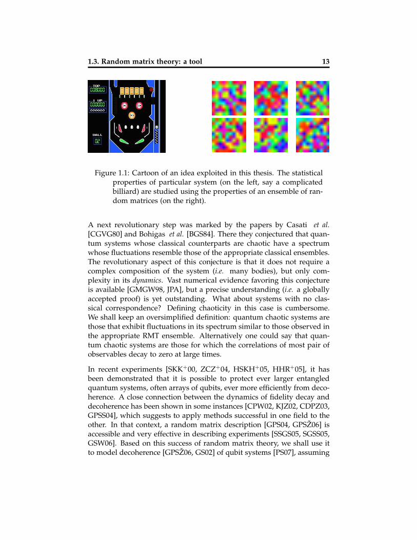
Figure 1.1: Cartoon of an idea exploited in this thesis. The statisticalproperties of particular system (on the left, say a complicatedbilliard) are studied using the properties of an ensemble of ran-dom matrices (on the right).
A next revolutionary step was marked by the papers by Casati et al.[CGVG80] and Bohigas et al. [BGS84]. There they conjectured that quan-tum systems whose classical counterparts are chaotic have a spectrumwhose fluctuations resemble those of the appropriate classical ensembles.The revolutionary aspect of this conjecture is that it does not require acomplex composition of the system (i.e. many bodies), but only com-plexity in its dynamics. Vast numerical evidence favoring this conjectureis available [GMGW98, JPA], but a precise understanding (i.e. a globallyaccepted proof) is yet outstanding. What about systems with no clas-sical correspondence? Defining chaoticity in this case is cumbersome.We shall keep an oversimplified definition: quantum chaotic systems arethose that exhibit fluctuations in its spectrum similar to those observed inthe appropriate RMT ensemble. Alternatively one could say that quan-tum chaotic systems are those for which the correlations of most pair ofobservables decay to zero at large times.
In recent experiments [SKK+00, ZCZ+04, HSKH+05, HHR+05], it hasbeen demonstrated that it is possible to protect ever larger entangledquantum systems, often arrays of qubits, ever more efficiently from deco-herence. A close connection between the dynamics of fidelity decay anddecoherence has been shown in some instances [CPW02, KJZ02, CDPZ03,GPSS04], which suggests to apply methods successful in one field to theother. In that context, a random matrix description [GPS04, GPSZ06] isaccessible and very effective in describing experiments [SSGS05, SGSS05,GSW06]. Based on this success of random matrix theory, we shall use itto model decoherence [GPSZ06, GS02] of qubit systems [PS07], assuming

14 Chapter 1. Introduction and fundamental tools
complicated dynamics in the environment, and a complicated coupling(in the interaction picture).
Three perspectives make such a random matrix treatment particularlyattractive. First, reduction of decoherence may, in some instances, beachieved by isolating some “far” environment (including spontaneousdecay) to a degree that it can, to first approximation, be neglected. Then itcan happen that the Heisenberg time of the relevant “near” environmentis finite on the time scale of decoherence. In such a case it becomesrelevant that RMT shows, in linear response approximation, a transitionfrom linear to quadratic decay at times of the order of the Heisenbergtime. This behavior is seen with spin chain environments [see sec. 5], andis essential for the success of the theory in describing the above mentionedexperiments of fidelity decay. Note also that the concept of a two stageenvironment has been used for basic considerations [Zur03]. Second, thelong term goal must be to describe in one theory the decay of fidelitythat includes undesirable deviations of the internal Hamiltonian of thecentral system (already done), together with decoherence (done in thisthesis). Third, random matrix descriptions include some aspects of chaosor mixing that are essential in the above experiments and may be usefulfor application to quantum computing [PZ01, FFS04, CPZ05].
For some technical aspects of random matrix theory, including Heisen-berg time, GOE and GUE ensembles, form factor and density of states,please go to appendix E.
Chapter 2
One qubit decoherence
In this chapter we analyze decoherence of a single qubit. We focus onweak coupling of the qubit to an environment. We shall use the cor-relation function approach proposed for purity decay in echo-dynamics[PS02], treating the coupling as the perturbation. The linear responseapproximation will be sufficient. In this approximation the ensemble av-erages, which we have to take in any RMT model, are feasible thoughsomewhat tedious. Exact solutions, which exist in some instances for thedecay of the fidelity amplitude [SS05, GKP+06], seem to be out of reachat present, because they require the evaluation of four-point functions.
The general program is as follows. Assume that the qubit is initially ina pure state, and evolves under its own local Hamiltonian. The qubit iscoupled via a random matrix to a large environment in turn describedby another random matrix. The coupling to the environment gives rise todecoherence. Averaging both the coupling and the environment Hamilto-nian over the RMT ensembles yields the generic behavior of decoherenceof the qubit.
We present a detailed analysis using both the Gaussian unitary (GUE)and the Gaussian orthogonal (GOE) ensembles [Car35, Meh91] for thedescription of the environment and the coupling. The two ensemblescorrespond to time reversal invariance (TRI) breaking and conserving dy-namics respectively.
In sec. 2.1 we shall state the model, recall the linear response formalismfor echo dynamics, and show how it can be adapted to forward evolu-
15
16 Chapter 2. One qubit decoherence
tion. In sec. 2.2 we discuss how to express the problem in terms of echodynamics. In sec. 2.3 we give the general solution, arising from the calcu-lations done in the appendix A. The analysis for the GUE case is given in2.4, whereas the one for the GOE is given in 2.5.
2.1 The model
We describe decoherence by considering explicitly additional degrees offreedom (henceforth called “environment”) which are interacting withthe qubit. The Hilbert space studied in this section is
H = H1 ⊗He, (2.1)
whereH1 (of dimension two) andHe (of dimension Ne) denote the Hilbertspaces of the qubit and the environment, respectively. The Hamiltonianis of the following form
Hλ = H1 ⊗ 11e + 111 ⊗ He + λV1,e (2.2)≡ H1 + He + λV1,e . (2.3)
Here, H1 represents the Hamiltonian acting on the qubit, He the Hamil-tonian of the environment, and V1,e the coupling between the qubit andthe environment. Notice how the indices in the operators indicate thespaces in which they act. The real parameter λ controls the strength ofthe coupling. We shall study the time evolution of an initially pure andseparable state
|ψ(t = 0)〉 = |ψ1〉 ⊗ |ψe〉 , (2.4)
where |ψ1〉 ∈ H1 and |ψe〉 ∈ He. At any time t, the state of the whole sys-tem is thus |ψ(t)〉 = exp(−itHλ)|ψ(0)〉, and the state of the single qubitis tre |ψ(t)〉〈ψ(t)|. As time evolves, the qubit and the environment getentangled, which means that after tracing out the environmental degreesof freedom, the state of the qubit becomes mixed.
At this point we wish to compare this model with the spectator model.We can arrive to the one studied in this chapter from two different direc-tions. One is if we eliminate the spectator. The other is if we consider aseparable (with respect to the spectator) situation [i.e. if in eq. (1.15) welet |ψc〉 = |ψs〉 ⊗ |ψi〉].
We describe both the coupling and the dynamics in the environmentwithin random matrix theory. To this end, He and Ve,1 are chosen both

2.2. Echo dynamics and linear response theory 17
from either the GUE or the GOE, depending on whether we wish to de-scribe a TRI breaking or TRI conserving situation. The Hamiltonian H1implies another free parameter of the model, namely the level splitting∆ of the two level system representing the qubit. While the state of thequbit |ψ1〉 implies more free parameters in our model, we assume thestate of the environment |ψe〉 to be random. This means that the state ischosen from an ensemble which is invariant under unitary transforma-tions, and is fully consistent with our minimum information assumption.In practice, this means that the coefficients are chosen as complex randomGaussian variables, and subsequently the state is normalized.
2.2 Echo dynamics and linear response theory
We shall calculate the value of purity as a function of time analytically,in a perturbative approximation. As we want to use the tools developedin the appendix A for a linear response formalism in echo dynamics, wemust state the problem in this language. To perform this task it is usefulto consider the above Hamiltonian [eq. (2.2)], as composed by an unper-turbed part H0 and a perturbation λV. The unperturbed part correspondsto the operators that act on each individual subspace alone whereas theperturbation corresponds to the coupling among the different subspaces;i.e. H0 = He + H1 and V = Ve,1.
We write the Hamiltonian as
Hλ = H0 + λV, (2.5)
and introduce the evolution operator and the echo operator defined by
Uλ(t) = e−iHλt, Mλ(t) = U0(t)†Uλ(t), (2.6)
respectively (h = 1 during all the thesis). The echo operator receives itsname because it evolves a state forward in time with a perturbed operatorand backwards with an unperturbed one. For the calculation of purityat a given time t, we replace the forward evolution operator Uλ by thecorresponding echo operator Mλ. Even though the resulting states aredifferent, i.e.
ρ(t) = tre,e′ Uλ(t)ρU†λ(t) 6= ρM(t) = tre,e′ Mλ(t)ρM†
λ(t), (2.7)
18 Chapter 2. One qubit decoherence
they are still related by the local (in the qubit and the environment) uni-tary transformation U0(t). Since local transformations do not change theentanglement properties, it holds (exactly!) that
P(t) = P[ρ(t)] = P[ρM(t)]. (2.8)
This step is crucial, since the echo operator admits a series expansion withmuch larger range of validity (both, in time and perturbation strength).However the numerical simulations are all done with forward evolutionalone as they require less computational effort.
The Born expansion of the echo operator up to second order reads
Mλ(t) = 11− iλI(t)− λ2 J(t) + O(λ3), (2.9)
with
I(t) =∫ t
0dτV(τ), J(t) =
∫ t
0dτ∫ τ
0dτ′V(τ)V(τ′) (2.10)
and V(t) = U0(t)†VU0(t) being the coupling in the interaction picture.Using this expansion we calculate the purity of the central system, aver-aged over the coupling and the Hamiltonian of the environment.
The reader must notice that at no point we used that the dimension of thecentral system is 2. In fact, we only required the locality of the operatorU0 and the fact that Mλ(t) ≈ 11. Thus, all this reasoning (in particulareqs. 2.8, 2.9, and 2.10) is equally valid for a completely general spectatorconfiguration or even more general configurations to be introduced later.
2.3 The solution
In appendix A, we compute the average purity 〈P(t)〉 as a function oftime in the linear response approximation eq. (2.9), following the stepsoutlined in sec. 2.2. The average is taken with respect to the coupling V1,e[using eqs. E.4 and E.5], the random initial state |ψe〉, and the spectrumof He. In the limit of Ne → ∞, we obtain [eq. (A.8), eq. (A.36)]
〈P(t)〉 = 1− 2 λ2∫ t
0dτ∫ t
0dτ′ Re AJI(τ, τ′) + O(λ4), (2.11)
with
AJI(τ, τ′) = [C1(|τ− τ′|)− S1(τ− τ′)]C(|τ− τ′|)+ χGOE[1− S′1(−τ− τ′)],(2.12)
2.4. The GUE case 19
where χGOE = 1 for the TRI case, and χGOE = 0 for the non-TRI case.The correlation functions C1(τ), S1(τ), S′1(τ), and C(τ) are defined in ap-pendix A.5. The first three depend on the state of the central system.Note that S′1(τ) is only relevant in the case of a GOE, and curiously is notstrictly a correlation function as it contains a dependence on the sum ofboth times. The last one, C(τ) deserves special attention, since it dependson the spectral properties of the environment determined by the function
1Ne
⟨∣∣∣∑Nej=1e−iEjt
∣∣∣2⟩ = C(t) = 1 + δ(t/τH)− b(β)2 (t/τH), (2.13)
(recall eq. (E.8) and subsequent equations). Here the Ej’s are the eigenen-ergies of He and τH is the corresponding Heisenberg time. Actually thevalidity of eq. (2.11) is not dependent on the environment being repre-sented by a GOE (β = 1) or GUE (β = 2). For these the two-point formfactor b(β)
2 is well known [Meh91] but any ensemble with the correspond-ing invariance properties will do, for example the POE or PUE [DRS91].
We first study the GUE case with and without an internal Hamiltoniangoverning the qubit. The next step is to work out the GOE case. Therewe concentrate on the case with no internal Hamiltonian governing in thequbit since we want to keep the discussion as simple as possible to focuson the consequences of the weaker invariance properties of the ensemble.
2.4 The GUE case
We are now in the position to give an explicit formula for 〈P(t)〉 in theGUE case. This formula will generally depend on some properties ofthe initial condition |ψ1〉. We wish to write it in the most general way.However the symmetries involved in the problem reduce the number ofparameters needed to describe the initial state |ψ1〉.
Recall that H = He + H1 + λV represents an ensemble of Hamiltonians inwhich He and V are chosen from GUEs of dimension Ne and 2Ne respec-tively, whereas H1 together with the initial condition |ψ1〉 remain fixedthroughout the calculation. The operations under which the ensemble isinvariant are local (with respect to the partitioning of the Hilbert spaceinto H1 and He), unitary (due to the invariance properties of the GUE),and leave H1 invariant. Hence the transformation matrices must be of the
20 Chapter 2. One qubit decoherence
formU ⊗ exp(iαH1) (2.14)
with α a real number and U a unitary operator acting onHe. The solutionmust also be invariant under that transformation.
This freedom allows to choose a convenient basis to solve the problem.On the one hand, it allows to write H0 in diagonal form (as done duringthe discussion of appendix A), and on the other hand, we can use it torepresent the initial state of the qubit in such a way that there is no phaseshift between the two components of the qubit. This can be achieved byappropriately choosing α in eq. (2.14). We thus write, without loosinggenerality
|ψ1〉 = cos φ|0〉+ sin φ|1〉 , (2.15)
where |0〉 and |1〉 are eigenstates of H1. Notice that if φ ∈ {0, π/2},|ψ1〉 is an eigenstate of H1. Finally, we choose the origin of the energyscale in such a way that the Hamiltonian of the qubit can be written asH1 = (∆/2)|0〉〈0| − (∆/2)|1〉〈1|.
We obtain the average purity from the general expression in eq. (2.11) andeq. (2.12). For a pure initial state ρ1 = |ψ1〉〈ψ1| the relevant correlationfunctions Re C1(τ), S1(τ), and C(τ) are given in eq. (A.46), eq. (A.48), andeq. (A.41), respectively. Using the symmetry of the resulting integrandwith respect to the exchange of τ and τ′, we find
〈P(t)〉 = 1− 4λ2∫ t
0dτ∫ τ
0dτ′ C(τ′)
[1− gφ (1− cos ∆τ′)
]+ O(λ4, N−1
e )
(2.16)with
gφ = cos4 φ + sin4 φ =3 + cos(4φ)
4(2.17)
quantifying the “distance” between |ψ〉 and an eigenbasis of H1.
Let us consider the following two limits for H1. The “degenerate limit”,where the level splitting ∆ is much smaller than the mean level spac-ing de = 2π/τH of the environmental Hamiltonian, and the “fast limit”,where the level splitting is much larger. In the latter case, the internalevolution of the qubit is fast compared with the evolution in the environ-ment. (We shall refer to these limits also in later sections.)
The degenerate limit leads to the known formula [PS07]
PD(t) = 1− λ2 fτH(t), (2.18)

2.4. The GUE case 21
with
fτH(t) = 2t max{t, τH}+2
3τH(min{t, τH})3. (2.19)
The result does not depend on the initial state of the qubit. Due to thedegeneracy all states are eigenstates of H1 and thus equivalent. The lead-ing term of the purity decay is linear before the Heisenberg time andquadratic after the Heisenberg time. Similar features were already ob-served in fidelity decay and purity decay in other contexts [GPSZ06].
In the fast limit (∆ � de), purity is obtained from eq. (2.16) by replacingcos ∆τ′ by 1 when it is multiplied with the δ function [see eq. (2.13)], andby zero everywhere else. For finite Ne care must be taken, since we areassuming Zeno time (which is given by the “width of the δ-function”) tobe much smaller than all other time scales, such that ∆ � Ne de. Theresulting expression is
PF(t) = 1− λ2[(1− gφ) fτH(t) + 2gφtτH] . (2.20)
Typically (unless |ψ1〉 is an eigenstate), this formula displays a domi-nantly linear decay below the Heisenberg time, and a dominantly quadraticdecay above, similar to eq. (2.18).
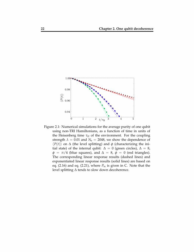
In fig. 2.1 we compare numerical simulations of the average purity 〈P(t)〉(symbols) with the corresponding linear response result (dashed lines)based on eqs. eq. (2.18) and eq. (2.20). The numerical results are obtainedfrom Monte Carlo simulations with 15 different Hamiltonians and 15 dif-ferent initial conditions for each Hamiltonian. We wish to underline twoaspects. First, the energy splitting in general leads to an attenuation ofpurity decay. Even though a strict inequality only holds for the limitingcases, PF(t) > PD(t) (for t 6= 0), we may still say that increasing ∆ tends toslow down purity decay. This result is in agreement with earlier findingson the stability of quantum dynamics [PZ02]. Second, for the fast limitand an eigenstate of H1 (gφ = 1) we find linear decay even beyond theHeisenberg time. A similar behaviour has been obtained in [GPSZ06], butthere an eigenstate of the whole Hamiltonian was required.
In [PS07] it was shown that exponentiation of the linear response resultleads to very good agreement beyond the validity of the original approx-imation. We use the formula eq. (C.1)
PELR(t) = P∞ + (1− P∞) exp[−1− PLR(t)
1− P∞
]. (2.21)
22 Chapter 2. One qubit decoherence
〈P(t
)〉
t/τH1 2 3 4 50
1.00
0.98
0.96
0.94
Figure 2.1: Numerical simulations for the average purity of one qubitusing non-TRI Hamiltonians, as a function of time in units ofthe Heisenberg time τH of the environment. For the couplingstrength λ = 0.01 and Ne = 2048, we show the dependence of〈P(t)〉 on ∆ (the level splitting) and φ (characterizing the ini-tial state) of the internal qubit: ∆ = 0 (green circles), ∆ = 8,φ = π/4 (blue squares), and ∆ = 8, φ = 0 (red triangles).The corresponding linear response results (dashed lines) andexponentiated linear response results (solid lines) are based oneq. (2.16) and eq. (2.21), where P∞ is given in C. Note that thelevel splitting ∆ tends to slow down decoherence.
2.5. The GOE case 23
where PLR(t) is truncation to second order in λ of the expansion eq. (2.16),and P∞ = 1/2 the estimated asymptotic value of purity for t → ∞, seeappendix C. From fig. 2.1 we see that the exponentiation indeed increasesthe accuracy of the bare linear response approximation.
2.5 The GOE case
We drop H1 for a moment, leaving H0 = He, resulting in
Hλ = He + λV. (2.22)
He is chosen from a GOE of dimension Ne and acts on He; V is chosenfrom a GOE of dimension 2Ne and acts onHe⊗H1. The resulting ensem-ble of Hamiltonians is invariant under local orthogonal transformations.In the qubit this invariance allows rotations of the kind exp(iασy) ∈ O(2).If such transformations are represented on the Bloch sphere, they becomerotations around the y axis. Hence, they can take any point on the Blochsphere onto the xy-plane. Supposing this point represents the initial state,it shows that we may assume the initial state in the qubit to be of the form
|ψ1〉 =|0〉+ eiγ|1〉√
2. (2.23)
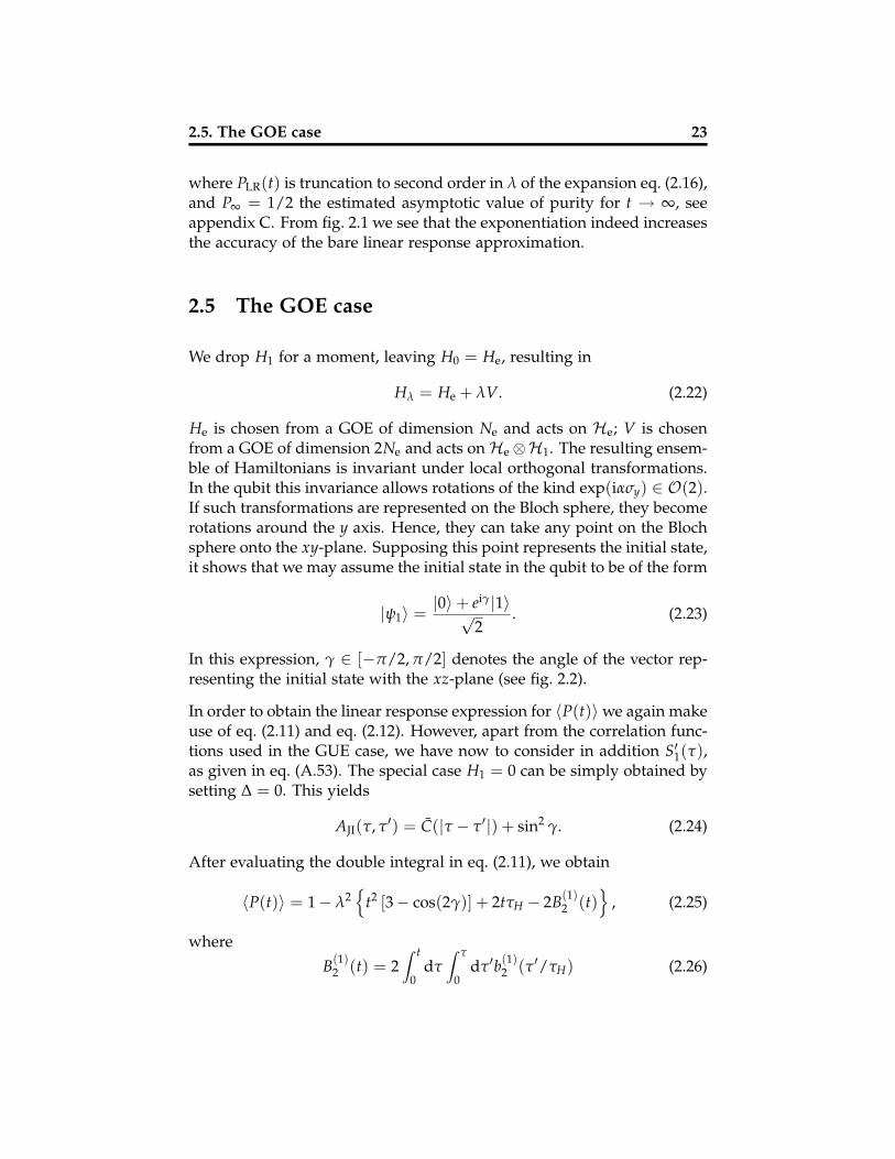
In this expression, γ ∈ [−π/2, π/2] denotes the angle of the vector rep-resenting the initial state with the xz-plane (see fig. 2.2).
In order to obtain the linear response expression for 〈P(t)〉we again makeuse of eq. (2.11) and eq. (2.12). However, apart from the correlation func-tions used in the GUE case, we have now to consider in addition S′1(τ),as given in eq. (A.53). The special case H1 = 0 can be simply obtained bysetting ∆ = 0. This yields
AJI(τ, τ′) = C(|τ − τ′|) + sin2 γ. (2.24)
After evaluating the double integral in eq. (2.11), we obtain
〈P(t)〉 = 1− λ2{
t2 [3− cos(2γ)] + 2tτH − 2B(1)2 (t)
}, (2.25)
where
B(1)2 (t) = 2
∫ t
0dτ∫ τ
0dτ′b(1)
2 (τ′/τH) (2.26)

24 Chapter 2. One qubit decoherence
Figure 2.2: Any pure initial state of the qubit can be mapped onto theBloch sphere. Here, we show the angle γ defined in eq. (2.23) incolor code. Regions of a given color represent subspaces whichare invariant under the transformation exp(iασy).
is the double integral of the form factor. It can be computed analytically,but the resulting expression is very involved [GPS04]. For our purposeit is sufficient to note that for t � τH, B(1)
2 (t) ∝ t3 (as in the GUE case),whereas for t � τH, t− B(1)
2 (t) grows only logarithmically. Thus it has asimilar behavior as in the GUE case, eq. (G.6).
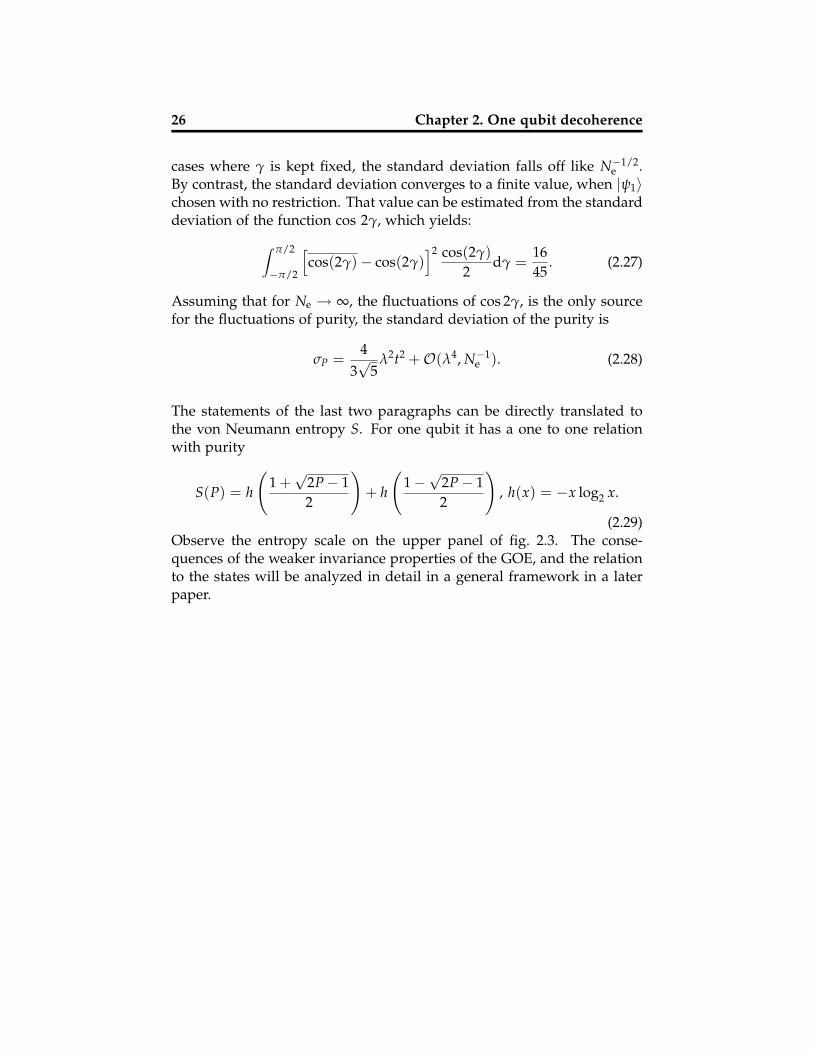
In fig. 2.3 we show 〈P(t)〉 for γ = 0 (green squares), for γ = π/2 (bluecircles), and for random values in the whole Bloch sphere (red triangles).In contrast to the GUE case in the degenerate limit, the average puritydepends on the initial state (via the angle γ). The fastest decay of purity isobserved for γ = π/2, where the image under the time reversal operationbecomes orthogonal to the initial state. The slowest decay is observed forγ = 0, which characterizes states which remain unchanged under thetime reversal symmetry operation. In the lower panel we show numericalresults for the standard deviation of the purity as a function of Ne, thedimension of the Hilbert space of the environment. We consider the samecases as on the upper panel: random initial states |ψ1〉 with fixed γ = 0(green squares), with fixed γ = π/2 (blue circles) and random states|ψ1〉 uniformly distributed on the Bloch sphere (red triangles). Note thatalong with the random choice of |ψ1〉, also He, V1,e, and |ψe〉 are randomlychosen from their respective ensembles. We clearly see that for those

2.5. The GOE case 25
1 2 3 4 5 6
0.996
0.997
0.998
0.999
1.000
0.005
0.01
0.015
0.02
0
t/τH
〈P(t
)〉
S
3 4 5 6 7 8 9 10 11
-13
-12
-11
-10
-9
log 2
σP
log2 Nenv
Figure 2.3: We display the behavior of purity and von Neumann en-tropy, in different regions in the Bloch sphere connected by or-thogonal transformations, characterized by γ in eq. (2.23). Onthe top figure we see the enveloping curve after running 100 ini-tial conditions (thick regions), their average (symbols) and thepredicted behavior (solid curves) by eq. (2.25). If γ = 0 we usecolor green; if γ = π/2 we use blue; and if we allow arbitraryγ we use red. In the lower panel σ is plotted for t = 40. We usethe same coding as the upper figure. For a fixed value of γ (blueand green) there is asymptotic self averaging whereas for an ar-bitrary initial condition (red) the standard deviation reaches thefinite value predicted in eq. (2.28), plotted as a horizontal line.We fixed λ = 10−3. A line ∝ 1/
√Ne is also included.
26 Chapter 2. One qubit decoherence
cases where γ is kept fixed, the standard deviation falls off like N−1/2e .
By contrast, the standard deviation converges to a finite value, when |ψ1〉chosen with no restriction. That value can be estimated from the standarddeviation of the function cos 2γ, which yields:∫ π/2
−π/2
[cos(2γ)− cos(2γ)
]2 cos(2γ)2
dγ =1645
. (2.27)
Assuming that for Ne → ∞, the fluctuations of cos 2γ, is the only sourcefor the fluctuations of purity, the standard deviation of the purity is
σP =4
3√
5λ2t2 +O(λ4, N−1
e ). (2.28)
The statements of the last two paragraphs can be directly translated tothe von Neumann entropy S. For one qubit it has a one to one relationwith purity
S(P) = h
(1 +√
2P− 12
)+ h
(1−√
2P− 12
), h(x) = −x log2 x.
(2.29)Observe the entropy scale on the upper panel of fig. 2.3. The conse-quences of the weaker invariance properties of the GOE, and the relationto the states will be analyzed in detail in a general framework in a laterpaper.

Chapter 3
Two qubit decoherence
In this chapter, we address the question whether entanglement withina given system affects its decoherence rate. In particular, as the namesuggests, we are going to study two qubit decoherence. We will usethe spectator model described in sec. 1.2. Moreover we shall considerthe first nontrivial example thereof, in the sense that the spectator spaceplays a nontrivial roll. However it is still the simplest example allowingthis possibility as both the spectator and the interacting space are qubits.We shall study two other configurations, namely when both qubits arecoupled to one or two environments. There, we shall start appreciatingthe power of the spectator model; we are going to be able to express theredecoherence in terms of the decoherence in the spectator configuration.
We will base our arguments on the calculations made in appendix A andthe results discussed in the previous chapter. Again we are going tostudy the linear response regime, and test with Monte Carlo simulationsthe validity of a heuristic exponentiation. The symmetries of the clas-sical ensembles will continue to play an important role to simplify theproblem. Moreover we shall find that entanglement has the property oftransporting the symmetry from one qubit to the other.
We first describe the models (configurations) we are going to study, sec. 3.1.Next we analyze in detail the results for the simplest configuration, thespectator model for two qubits, sec. 3.2. There we consider both the GUEand GOE cases. We then generalize the result to the other configurationsin sec. 3.3 and sec. 3.4.
27

28 Chapter 3. Two qubit decoherence
He
H1H1H1 H2 H2 H2
(b)(a) (c)
He He′ He
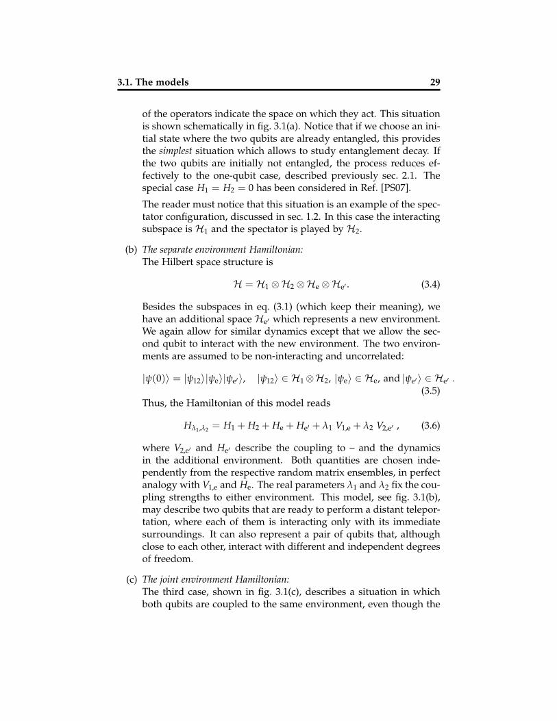
Figure 3.1: Schematic representations of the different dynamical con-figurations studied in this article: (a) the 2 qubit spectatorHamiltonian, (b) the separate, and (c) the joint environmentHamiltonian.
3.1 The models
For the two qubit case, the Hilbert space structure must be slightly morecomplicated than eq. (2.1). We need at least to provide the Hilbert spacefor a second qubit, and, in one of the models, we shall need an additionalHilbert space for a second environment. In all cases the initial conditionis pure in the central system, but the two qubits can share some entangle-ment. We shall consider three different dynamical scenarios, all explicitlyexcluding any interaction between the two qubits:
(a) The 2 qubit spectator Hamiltonian:The Hilbert space structure is
H = H1 ⊗H2 ⊗He. (3.1)
BothH1 andH2 are the state spaces of the qubits (dimH1 = dimH2 =2) and He (of dimension Ne) is the state space of an environment.The central system is, obviously,
Hc = H1 ⊗H2. (3.2)
Only the first qubit is coupled to an environment, and we allow forlocal dynamics. The total Hamiltonian reads
Hλ = H1 + H2 + He + λV1,e , (3.3)
where λ is again a real number modulating the strength of the cou-pling. We recall the remark in sec. 1.2, namely that the sub-indices
3.1. The models 29
of the operators indicate the space on which they act. This situationis shown schematically in fig. 3.1(a). Notice that if we choose an ini-tial state where the two qubits are already entangled, this providesthe simplest situation which allows to study entanglement decay. Ifthe two qubits are initially not entangled, the process reduces ef-fectively to the one-qubit case, described previously sec. 2.1. Thespecial case H1 = H2 = 0 has been considered in Ref. [PS07].
The reader must notice that this situation is an example of the spec-tator configuration, discussed in sec. 1.2. In this case the interactingsubspace is H1 and the spectator is played by H2.
(b) The separate environment Hamiltonian:The Hilbert space structure is
H = H1 ⊗H2 ⊗He ⊗He′ . (3.4)
Besides the subspaces in eq. (3.1) (which keep their meaning), wehave an additional space He′ which represents a new environment.We again allow for similar dynamics except that we allow the sec-ond qubit to interact with the new environment. The two environ-ments are assumed to be non-interacting and uncorrelated:
|ψ(0)〉 = |ψ12〉|ψe〉|ψe′〉, |ψ12〉 ∈ H1⊗H2, |ψe〉 ∈ He, and |ψe′〉 ∈ He′ .(3.5)
Thus, the Hamiltonian of this model reads
Hλ1,λ2 = H1 + H2 + He + He′ + λ1 V1,e + λ2 V2,e′ , (3.6)
where V2,e′ and He′ describe the coupling to – and the dynamicsin the additional environment. Both quantities are chosen inde-pendently from the respective random matrix ensembles, in perfectanalogy with V1,e and He. The real parameters λ1 and λ2 fix the cou-pling strengths to either environment. This model, see fig. 3.1(b),may describe two qubits that are ready to perform a distant telepor-tation, where each of them is interacting only with its immediatesurroundings. It can also represent a pair of qubits that, althoughclose to each other, interact with different and independent degreesof freedom.
(c) The joint environment Hamiltonian:The third case, shown in fig. 3.1(c), describes a situation in whichboth qubits are coupled to the same environment, even though the
30 Chapter 3. Two qubit decoherence
coupling matrices are still independent. The Hilbert space is iden-tical to the one for the 2 qubit spectator configuration. The totalHamiltonian reads
Hλ1,λ2 = H1 + H2 + He + λ1 V1,e + λ2 V2,e , (3.7)
where V2,e describes the coupling of the second qubit to the envi-ronment. It is chosen independently from the same random matrixensemble as V1,e.
3.2 The spectator Hamiltonian
The first step to calculate the decoherence of the initial state
$0 = |ψ12〉〈ψ12| ⊗ |ψe〉〈ψe|, (3.8)
evolved with the Hamiltonian (3.3), is to realize that the echo operatordoes not contain H2. The quantum echo of $0 after time t is
$M(t) =[
112 ⊗Mλ(t)]$0
[112 ⊗M†
λ(t)]. (3.9)
Since $M(t) remains a pure state in H1 ⊗H2 ⊗He,
P(t) = tr ρc(t)2 = tr ρe(t)2 (3.10)
with ρc(t) = tre $M(t) and ρe(t) = trc $M(t). This simply means that,as a formality, we can calculate purity of the central system, calculatingpurity of the environment. As the echo operator acts as the identity onthe second qubit,
ρe(t) = tr1 Mλ(t)(tr2 $0)M†λ(t) (3.11)
= tr1 Mλ(t) (ρ1 ⊗ |ψe〉〈ψe|) M†λ(t),
where ρ1 = tr2 |ψ12〉〈ψ12|.
We may therefore compute the purity of the spectator model, withoutever referring explicitly to the second qubit! Any dependence of the decayof purity on the central system as a whole is encoded into the initialdensity matrix ρ1. This also implies that we can use the results obtainedin A, and hence eq. (2.11) and eq. (2.12) remain valid. The only differenceis that for the correlation functions C1(τ), S1(τ), and S′1(τ), we now have

3.2. The spectator Hamiltonian 31
to insert the respective expressions which apply for mixed initial statesof the first qubit. These expressions are given in A.5. We stress, for laterreference, that this line of reasoning is not limited by the fact that theinteracting and spectator systems are qubits.
3.2.1 The GUE case
We wish to write the initial condition in its simplest form. We mustrespect the structure of the Hamiltonian (3.3). However we can still takeadvantage of all its invariance properties, when seen as an ensemble.Given a fixed H1, that ensemble of Hamiltonians is invariant under localoperations of the form
UNe ⊗ exp iαH1 ⊗U2 (3.12)
where UNe ∈ U (Ne) is any unitary operator acting on the environment,α a real number, and U2 ∈ U (2) is any unitary operator acting on thesecond qubit.
The freedom within the qubits allows to choose a basis {|0〉, |1〉}⊗{|0〉, |1〉}in which the initial state [see eq. (3.8)] can be written as
|ψ12〉 = cos θ(cos φ|0〉+ sin φ|1〉)|0〉+ sin θ(sin φ|0〉 − cos φ|1〉)|1〉, (3.13)
and still, H1 = ∆2 |0〉〈0| − ∆
2 |1〉〈1| is diagonal. Let us prove it in a construc-tive manner. To find this basis we start using the Schmidt decompositionto write
|ψ12〉 = cos θ|0102〉+ sin θ|1112〉 (3.14)
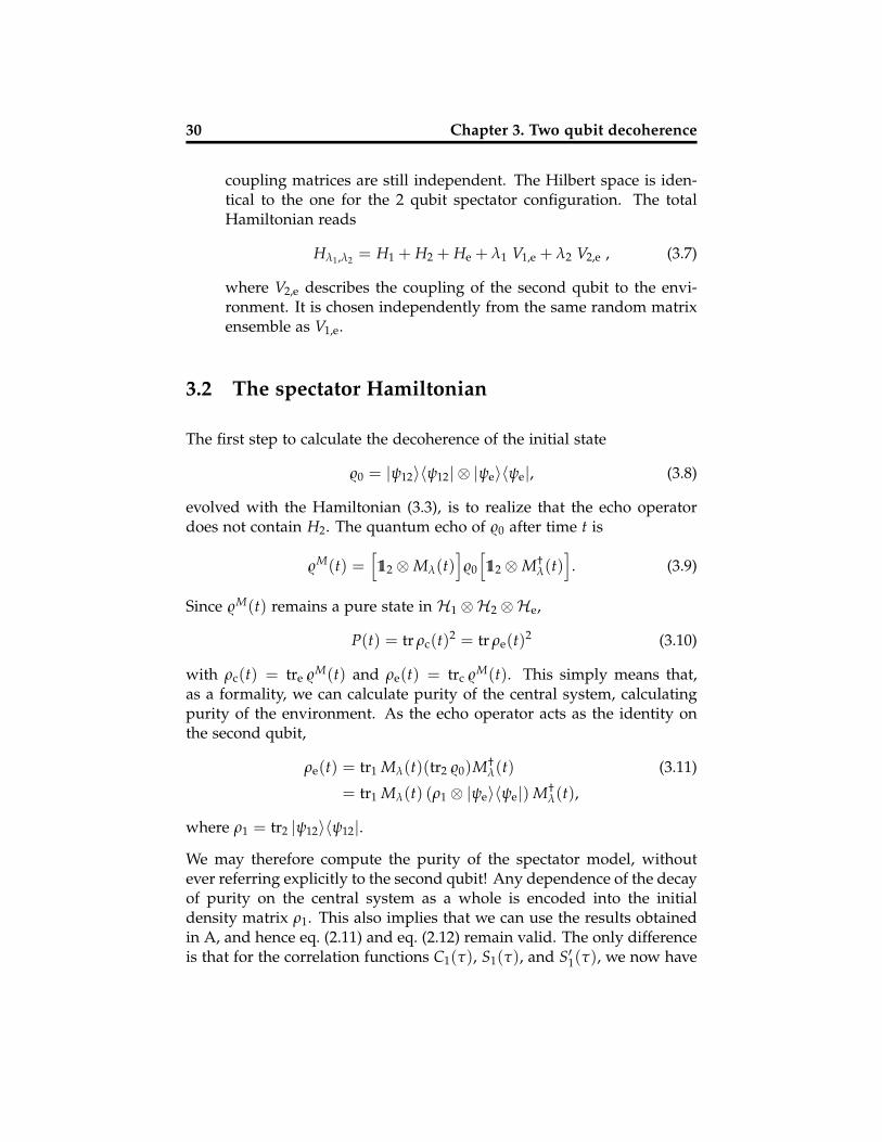
with {|0i〉, |1i〉} being an orthonormal basis of particle i. For the firstqubit, we fix the z axis of the Bloch sphere (containing both |0〉 and |1〉)parallel to the eigenvectors of H1, and the y axis perpendicular (in theBloch sphere) to both the z axis and |01〉. The states contained in the xzplane are then real superpositions of |0〉 and |1〉, which implies that
|01〉 = cos φ|0〉+ sin φ|1〉, (3.15)|11〉 = sin φ|0〉 − cos φ|1〉, (3.16)
for some φ. In the second qubit it is enough to set
|02〉 = |0〉, (3.17)|12〉 = |1〉. (3.18)
32 Chapter 3. Two qubit decoherence
(a) z
y
x
|0〉
|1〉
|11〉
|01〉
(b)
z
y
x
|0〉 = |02〉
|1〉 = |12〉
Figure 3.2: A figure to visualize the way the initial condition isparametrized, using the Bloch sphere, is presented. On the left,qubit one has an internal Hamiltonian. Its eigenvectors (|0〉 and|1〉) are represented in blue. The z axis is chosen parallel to |0〉.The x axis is chosen so that both |01〉 and |11〉 have real coeffi-cients; i.e. such that the xz plane contains |01〉 and |11〉. On theright we represent the second qubit. We have absolute freedomto choose the basis (even if an internal Hamiltonian is present),and thus we choose it according to the natural Schmidt decom-position.
This freedom is also related to the fact that purity only depends ontr2 |ψ12〉〈ψ12|. A visualization of this argumentation is found in fig. 3.2.The angle θ ∈ [0, π/4] measures the entanglement
C(|ψ12〉〈ψ12|) = sin 2θ (3.19)
whereas the angle φ ∈ [0, π/2] is related to an initial magnetization.
The general solution for purity using this parametrization is
P(t) = 1− 4λ2∫ t
0dτ∫ τ
0dτ′C(τ′)
[g(1)
θ,φ + g(2)θ,φ cos ∆τ′
]+ O(λ4, N−1
e ),
(3.20)where the geometric factors g(1)
θ,φ ∈ [0, 1/2], and g(2)θ,φ ∈ [1/2, 1] are ex-
pressed as
g(1)θ,φ = gθ(1− gφ) + gφ(1− gθ) (3.21)
g(2)θ,φ = 2(1− gθ)− gφ(1− 2gθ), (3.22)

3.2. The spectator Hamiltonian 33
0
0.2
0.4
0.6
0.8
1
0
π/4
π/4
π/8
π/2
g(1)θ,φ
0
π/4
π/4
π/8
π/2
g(2)θ,φ
00
θθ
φφ
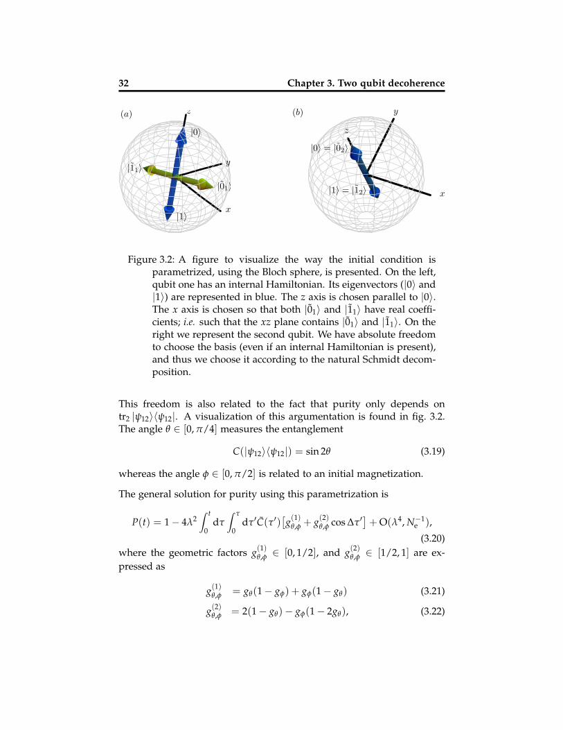
Figure 3.3: Visualization of the geometric factors g(1)θ,φ, and g(2)
θ,φ from
left to right respectively. For g(1)θ,φ we see that for pure eigenstates
of H1 its value is zero. This leads to a higher qualitative stabilityof this kind of states.
in terms of the functions gφ and gθ , defined in eq. (2.17). Both geometricfactors are shown in fig. 3.3. Eq. (3.20) is obtained from eq. (2.11) andeq. (2.12) by insertion of the eq. (A.46) and eq. (A.52) for Re C1(τ) andS1(τ), respectively.
We consider again two limits for ∆. In the degenerate limit (∆ � 1/τH)purity decay is given by
PD(t) = 1− λ2(2− gθ) fτH(t), (3.23)
where fτH(t) is defined in eq. (2.19). The result is independent of φ since adegenerate Hamiltonian is, in this context, equivalent to no Hamiltonianat all. The θ-dependence in this formula shows that an entangled qubitpair is more susceptible to decoherence than a separable one.
In the fast limit (∆� 1/τH) we get
PF(t) = 1− λ2[
g(1)θ,φ fτH(t) + 2τHg(2)
θ,φt]
. (3.24)
For initial states chosen as eigenstates of H1 we find linear decay of purityboth below and above Heisenberg time. In order for ρ1 to be an eigenstateof H1 it must, first of all, be a pure state (in H1). Therefore this behaviorcan only occur if θ = 0 or θ = π/2. Apart from that particular case,we observe in both limits, the fast as well as the degenerate limit, thecharacteristic linear/quadratic behavior before/after the Heisenberg timesimilar to the one qubit case.

34 Chapter 3. Two qubit decoherence
〈P(t
)〉
t/τH1 21.50.5 2.50
1.0
0.8
0.7
0.9
Separable, degenerate
Separable, fast
Bell, degenerate
Bell, fast
Figure 3.4: Numerical simulations for the average purity as a func-tion of time in units of the Heisenberg time of the environment(spectator configuration, GUE case). For the coupling strengthλ = 0.03 we show the dependence of 〈P(t)〉 on the level split-ting ∆ in H1 and on the initial degree of entanglement betweenthe two qubits (in all cases φ = π/4). For separable state (θ = 0)and a degenerate limit we use � whereas for the fast limit, with∆ = 8, we use N; For Bell states, the corresponding limits areencoded as • in the degenerate limit and � in the fast limit(∆ = 0.8). The corresponding linear response results (dashedlines) are based on eq. (3.23), eq. (3.24) and eq. (2.21). The expo-nentiated linear response results (solid lines) are obtained basedon the results of appendix C. The theoretical curves are plottedwith the same color, as the respective numerical data. In allcases Ne = 1024.
In fig. 3.4 we show numerical simulations for 〈P(t)〉. We average over30 different Hamiltonians each probed with 45 different initial condi-tions. We contrast Bell states (φ = π/4, θ = π/4) with separable states(φ = π/4, θ = 0), and also systems with a large level splitting (Ne �∆ = 8 � 1/τH) with systems having a degenerate Hamiltonian (∆ = 0).The results presented in this figure show that entanglement generally en-hances decoherence. This can be anticipated from fig. 3.3, since for fixedφ, increasing the value of θ (and hence entanglement) increases both g(1)
θ,φ
and g(2)θ,φ. At the same time we find again that increasing ∆ tends to re-
duce the rate of decoherence. A strict inequality only holds among thetwo limiting cases (just as in the one qubit case): From g(2)
θ,φ = 2− g(1)θ,φ− gθ ,
it follows that (PF− PD)/λ2 = g(2)θ,φ[ fτH(t)− 2tτH] ≥ 0. Therefore, for fixed
3.2. The spectator Hamiltonian 35
initial conditions and t greater than 0, PF(t) > PD(t). This is the secondaspect illustrated in fig. 3.4.
In order to extend the formulae to longer times/smaller purities we expo-nentiate them using the results of appendix C. The numerical simulations(see fig. 3.4) agree very well with that heuristic exponentiated linear re-sponse formula. In one case (blue rhombus) where the agreement is notas good, we found that it is the inaccurate estimate P∞ = 1/4 of theasymptotic value of purity, which leads to the deviations.
3.2.2 The GOE case
Let us consider the GOE average of both He and V1,e. When averagingHe and V1,e over the GOE, we are again confronted with the fact that theinvariance group is considerably smaller than in the GUE case. In thiscontext the initial entanglement between the two qubits has a crucial im-portance since it “transports” the invariance properties from the spectatorto the coupled qubit.
For the sake of simplicity, we focus on the degenerate limit setting H1 = 0.Note that on the basis of the results in appendix A, the general case canbe treated similarly and the corresponding result will be presented at theend of this subsection.
We first specify the operations under which the spectator Hamiltonianeq. (3.3), considered as a random matrix ensemble, is invariant. As both,the internal Hamiltonian of the environment and the coupling, are se-lected from the GOE the invariance operations form the group
O(Ne)×O(2)×U (2), (3.25)
and have the structure ONe ⊗ exp(iασy)⊗U2, with ONe being an orthog-onal matrix (acting in He), α a real number, and U2 a unitary operatoracting on the spectator qubit. The direct product structure of the invari-ance group obliges us to respect the identity of each particle, but allowsto analyze each qubit separately. For instance, if we replace the randomcoupling matrix V1,e with one which involves both qubits, the invariancegroup would be O(Ne)×O(4). As a consequence, purity decay wouldbecome independent of the entanglement within the qubit pair: for anyentangled state one can find an orthogonal matrix which maps the state

36 Chapter 3. Two qubit decoherence
onto a separable one 1.
We write the initial condition |ψ12〉 as in eq. (3.14). For the coupledparticle follows the same analysis made in sec. 2.5. We can thus write|01〉 = 2−1/2[|0〉 + exp(iγ)|1〉] and, in order to respect orthogonality,|11〉 = 2−1/2 exp(iζ)[|0〉 − exp(iγ)|1〉]. For the second qubit we have thesame complete freedom as in eq. (3.2.1). We thus select |02〉 = |0〉 and|12〉 = exp(−iζ)|1〉 to erase the relative phase in the first qubit and finallywrite the initial state as
|ψ12〉 =cos θ(|0〉+ eiγ|1〉)|0〉+ sin θ(|0〉 − eiγ|1〉)|1〉√
2. (3.26)
The average purity is still given by the double integral expression ineq. (2.11). However, in the present case the mixed initial state ρ1 =tr2 |ψ12〉〈ψ12| must be used. For ∆ = 0, the resulting integrand reads
AJI(τ, τ′) = (2− gθ)C(|τ − τ′|) + 1− gθ + (2gθ − 1) sin2 γ, (3.27)
where C(|τ − τ′|) is given in eq. (2.13). Evaluating the double integral,we obtain
〈P(t)〉 = 1− λ2{
t2[4− 2 cos2(2θ) cos2 γ] + (4− 2gθ)[tτH − B(1)
2 (t)]}
,(3.28)
where B(1)2 (t) is given in eq. (2.26). As in the GUE case, this result de-
pends on the entanglement of the initial state and, as in the one-qubitGOE case, it also depends on γ. Again it turns out that Bell states aremore susceptible to decoherence than separable states. Note however,that purity as a function of θ is not monotonous. Hence, a finite increaseof entanglement does not guarantee that the purity decreases everywherein time. For separable states, gθ = 1, we retrieve formula eq. (2.25). How-ever, for completely entangled states, θ = π/4 the dependence on γ islost. This is understood from a physical point of view, noticing thatany local unitary operation on a Bell state can be reduced to a single
1One can see a general state |ψ12〉 = ∑3i=0(ai + ibi)|i〉, ai, bi ∈ R as characterized by
2 real vectors ~a = (a0, a1, a2, a3),~b = O(b0, b1, b2, b3) ∈ R4. We can rotate ~a to a vectorhaving only the first component ~a′ = (a′0, 0, 0, 0) using an orthogonal matrix O. Considerthe vector~b′ = O~b rotated by the same transformation. We next repeat the procedure onthe last 3 axes (for ~b′) with an orthogonal transformation O′, to obtain a vector havingonly the first two components. We thus have, an orthogonal transformation that takes|ψ12〉 to O′O|ψ12〉 = ∑1
i=0(a′′i + ibi
′′)|i〉 = |01〉(α|02〉+ β|12〉, a separable state.

3.3. The separate environment Hamiltonian 37
local unitary operation acting on a single qubit. In other words, givenU1,2 = U1 ⊗U2, there exists a unitary U′1 such that
U1 ⊗U2|Bell〉 = U′1 ⊗ 11|Bell〉 (3.29)
(|Bell〉 is any 2 qubit pure state with C = 1, e.g. |00〉+ |11〉). We can thensay that the invariance properties in the coupled qubit are inherited fromthe spectator qubit via entanglement.
Let us obtain the standard deviation for the different possible initial con-ditions in the qubits. We want to analyze the situation separately for afixed value of concurrence. Then, as the invariant measure of the ensem-ble of initial conditions, and fixing the amount of entanglement, we shalluse the tensor product of the invariant measures in each of the qubits.Since there is no dependence of eq. (3.28) on the second qubit, the appro-priate invariant measure is trivially inherited from the invariant measurefor a single qubit. The resulting value for the standard deviation is
σP =4λ2t2 cos2(2θ)
3√
5. (3.30)
Based on the appendix A we can also obtain the average purity for ∆ 6=0. The parametrization of the initial states is more complicated sincetwo preferred directions arise, one from the eigenvectors of the internalHamiltonian and the other from the invariance group. The result can beexpressed in the form given in eq. (2.11), with
Re AJI(τ, τ′) = C(|τ − τ′|)[
g(1)θ,φ + g(2)
θ,φ cos ∆(τ − τ′)]
+ g(1)θ,φ − (1− g(2)
θ,φ) cos[∆(τ + τ′)− 2η] + O(λ4, N−1e ) .
The angle η is related to a phase shift between the components of any ofthe eigenvectors of the initial density matrix ρ1. Here we can again seethe term containing a sum of times, i.e. a term that is not a correlationfunction. However, this term is small, and adequate values must mechosen to see its effect. Still it is observable in numerical simulations,with moderate effort.
3.3 The separate environment Hamiltonian
We proceed to study purity decay with other configurations of the envi-ronment. Consider the separate environment configuration, pictured in
38 Chapter 3. Two qubit decoherence
fig. 3.1(b). The corresponding uncoupled Hamiltonian is
H0 = H1 + H2 + He + He′ (3.31)
and the coupling isλV = λ1Ve,1 + λ2Ve′,2. (3.32)
From now on we assume that the internal Hamiltonians of the environ-ment and the couplings are chosen from the GUE. The generalizationfor the GOE can be obtained along the same lines using the correspond-ing results of sec. 3.2.2. The initial condition has a separable structurewith respect to both environments, see eq. (3.5). The coupling in the in-teraction picture separates into two parts acting on different subspacesλV = λ1V(1) + λ2V(2), where
V(1) = ei(H1+He)Ve,1e−i(H1+He), V(2) = ei(H2+He′ )Ve′,2e−i(H2+He′ ). (3.33)
Notice that V(1) (V(2)) does not depend on He′ (He). Since V(1) and V(2)
are uncorrelated, quadratic averages separate as
λ2〈VijVkl〉 = λ21〈V(1)
ij V(1)kl 〉+ λ2
2〈V(2)ij V(2)
kl 〉. (3.34)
This leads to a natural separation of each of the contributions to purity
1− 〈P(t)〉 = 1− P(1)spec(t) + 1− P(2)
spec(t), (3.35)
where P(i)spec(t) denotes the average purity with particle i being a spectator,
as given in sec. 3.2. In this way, the problem formally reduces to that ofthe spectator model. The respective expressions in sec. 3.2 may be used.For instance, if we assume broken TRI, we obtain from eq. (3.20)
〈P(t)〉 = 1− 42
∑i=1
λ2i
∫ t
0dτ∫ τ
0dτ′
[g(1)
θ,φi+ g(2)
θ,φicos ∆iτ
′]
Ci(τ′)+ O(λ4, N−1e ),
(3.36)where C1 and C2 are the correlation functions of the corresponding envi-ronments defined in exact correspondence with eq. (2.13), for He and He′
respectively. If in one or both of the qubits, the level splitting in the inter-nal Hamiltonians is very large/small compared to the Heisenberg timein the corresponding environment (denoted by τe and τe′ for He and He′ ,respectively) the degenerate and/or fast approximations may be used. Asan example, if ∆1 � 1/τe and ∆2 � 1/τe′ we find
PD(t) = 1− (2− gθ)(λ21 fτe(t) + λ2
2 fτe′ (t)), (3.37)
3.4. The joint environment configuration 39
whereas if ∆1 � 1/τe and ∆2 � 1/τe′
PF(t) = 1− λ21
[g(1)
θ,φ1fτe(t) + 2τeg(2)
θ,φ1t]− λ2
2
[g(1)
θ,φ2fτe′ (t) + 2τe′g
(2)θ,φ2
t]
.(3.38)
It is interesting to note that if we have two separate but equivalent envi-ronments (i.e. both Heisenberg times are equal), we get exactly the sameresult as for a single environment. Also notice that the Hamiltonian ofthe entire system separates and thus the total entanglement of the twosubsystems (H1 ⊗He and H2 ⊗He′) becomes time independent.
3.4 The joint environment configuration
The last configuration we shall consider is the one of joint environment;see fig. 3.1(c). Its uncoupled Hamiltonian is
H0 = H1 + H2 + He (3.39)
whereas the coupling is given by
λV = λ1Ve,1 + λ2Ve,2. (3.40)
Notice the similarity with eq. (3.31) and eq. (3.32). However, as discussedin the introduction, they represent very different physical situations. Thecoupling in the interaction picture can again be split λV = λ1V(1) +λ2V(2), where
V(1) = ei(H1+He)Ve,1e−i(H1+He), V(2) = ei(H2+He)Ve,2e−i(H2+He). (3.41)
Note the slight difference with eq. (3.33). However V(1) and V(2) are stilluncorrelated, enabling us to write again eq. (3.34).
From now on, the calculation is formally the same as in the separateenvironment case. Hence we can inherit the result eq. (3.36) directly,taking into account that since they come from the same environmentalHamiltonian, the two correlation functions are the same. In case anyof the Hamiltonians fulfills the fast or degenerate limit conditions, thecorresponding expressions to eq. (3.37) and eq. (3.38) can be written. Asan example, if the first qubit has no internal Hamiltonian, and the secondone has a big energy difference, the resulting expression for purity decayis
〈P(t)〉 = 1− λ21(2− gθ) fτH(t)− λ2
2
[g(1)
θ,φ2fτH(t) + 2τHg(2)
θ,φ2t]+ O(λ4, N−1
e ),(3.42)

40 Chapter 3. Two qubit decoherence
where τH is the Heisenberg time of the joint environment. Monte Carlosimulations showing the validity of the result were done with satisfactoryresults, comparable to those obtained in fig. 3.4. The parameter rangechecked was similar to that in the figure.

Chapter 4
Entanglement decay
In the previous chapter we studied purity decay of two qubits. Puritymeasures entanglement with the environment, but we can wonder howdecoherence affects the internal quantum mechanical properties of thecentral system. Possibly the most important quantum mechanical prop-erty of a multi-particle system is its internal entanglement. As discussedin appendix D, a simple and meaningful measure of two qubit entan-glement is concurrence (C). Since concurrence is defined in terms of theeigenvalues of a Hermitian 4× 4-matrix, an analytical treatment, even inlinear response approximation, is much more involved than in the case ofpurity. A study along the same lines followed in the last chapters, is outof reach for the time being.
We shall first explore a relation (first found in [PS06], partly explained in[ZB05], and further studied in [PS07]) between concurrence and purity.We show that this relation is valid in a wide parameter range (sec. 4.1).Combining it with an appropriate formula for purity decay, we obtain ananalytic prediction for concurrence decay in sec. 4.2. We compare our pre-diction with Monte Carlo simulations. It is essential that the two qubitsdo not interact; otherwise the coupling between the qubits would act asan additional sink (or source) for internal entanglement – a complicationwe wish to avoid. In the last part of the section we extend our ideas tonon-Bell states.
41
42 Chapter 4. Entanglement decay
4.1 The CP plane
We study the relation between concurrence and purity using the CP-plane, where we plot concurrence against purity with time as a parame-ter. This plane is plotted in fig. 4.1. The gray area indicates the region ofphysically admissible states [MJWK01]. The upper boundary of this re-gion is given by the maximally entangled mixed states. This set dependson the entanglement measures chosen [WNG+03]. Large purity, i.e. lowentanglement with the environment, is required in order to have largeconcurrence, i.e. entanglement within the pair. This is a consequenceof the monogamy of entanglement. Note also that concurrence becomesidentically zero before purity reaches its minimum at 1/4. Another re-gion of interest, plotted in red in fig. 4.1(a), corresponds to those states(density matrices), which form the image of a Bell state under the set oflocal (i.e. acting separately on each qubit) unital operations [ZB05]. Uni-tal operations are those which preserve the identity [Key02]. Single qubitunital operations include bit flip and phase flip, whereas an example of anon-unital operation is amplitude damping [NC00]. Finally, the Wernerstates ρW = α 11
4 + (1− α)|Bell〉〈Bell|, 0 ≤ α ≤ 1, define a smooth curve onthe CP-plane (black solid line). The analytic form of this curve is [PS07]
CW(P) = max
{0,√
12P− 3− 12
}, (4.1)
and will be referred to as the Werner curve. Note that states mapped tothe Werner curve are not necessarily Werner states.
In fig. 4.1(b), we perform numerical simulations in the spectator configu-ration assuming broken time reversal symmetry (GUE case). We computethe average concurrence for a given interval of purity using 15 differentHamiltonians and 15 different initial states for each Hamiltonian. We fixthe level splitting in the coupled qubit to ∆ = 1 and consider two differentvalues λ = 0.02 and 0.14 for the coupling to the environment. Fig. 4.1(b)shows the resulting CP-curves for different dimensions of He. Observethat for both values of λ, the curves converge to a certain limiting curveas dim(He) tends to infinity. While for λ = 0.02, this curve is at a finitedistance of the Werner curve, for λ = 0.14 it practically coincides withCW(P). Varying the configuration, the coupling strength, the level split-ting, or the ensemble (GOE/GUE), gives the same qualitative results inthe CP plane, for large dimensions. In some cases we have an accumu-
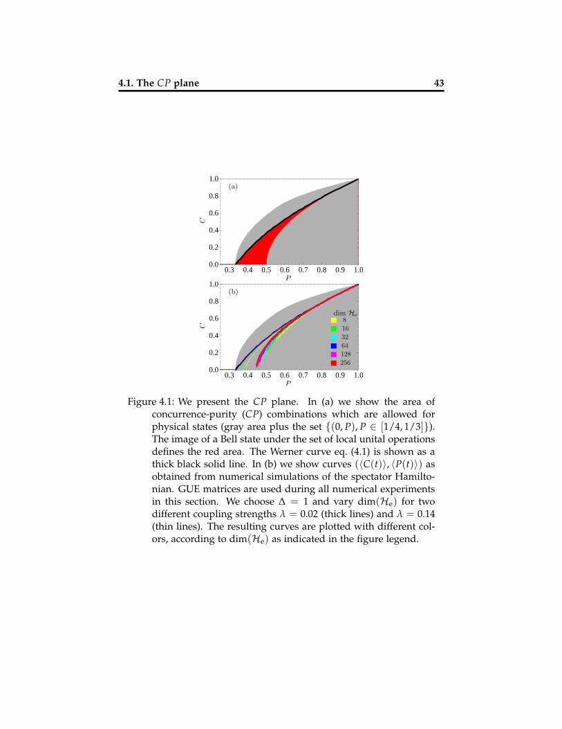
4.1. The CP plane 43
0.3 0.4 0.5 0.6 0.7 0.8 0.9 1.00.0
0.2
0.4
0.6
0.8
1.0(a)
P
C
0.3 0.4 0.5 0.6 0.7 0.8 0.9 1.00.0
0.2
0.4
0.6
0.8
1.0(b)
P
C
dim He8
16
32
64
128
256
Figure 4.1: We present the CP plane. In (a) we show the area ofconcurrence-purity (CP) combinations which are allowed forphysical states (gray area plus the set {(0, P), P ∈ [1/4, 1/3]}).The image of a Bell state under the set of local unital operationsdefines the red area. The Werner curve eq. (4.1) is shown as athick black solid line. In (b) we show curves (〈C(t)〉, 〈P(t)〉) asobtained from numerical simulations of the spectator Hamilto-nian. GUE matrices are used during all numerical experimentsin this section. We choose ∆ = 1 and vary dim(He) for twodifferent coupling strengths λ = 0.02 (thick lines) and λ = 0.14(thin lines). The resulting curves are plotted with different col-ors, according to dim(He) as indicated in the figure legend.
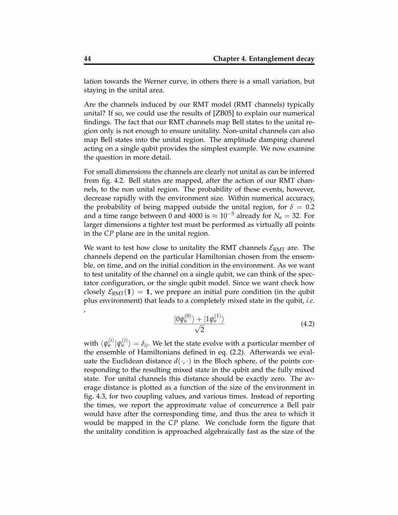
44 Chapter 4. Entanglement decay
lation towards the Werner curve, in others there is a small variation, butstaying in the unital area.
Are the channels induced by our RMT model (RMT channels) typicallyunital? If so, we could use the results of [ZB05] to explain our numericalfindings. The fact that our RMT channels map Bell states to the unital re-gion only is not enough to ensure unitality. Non-unital channels can alsomap Bell states into the unital region. The amplitude damping channelacting on a single qubit provides the simplest example. We now examinethe question in more detail.
For small dimensions the channels are clearly not unital as can be inferredfrom fig. 4.2. Bell states are mapped, after the action of our RMT chan-nels, to the non unital region. The probability of these events, however,decrease rapidly with the environment size. Within numerical accuracy,the probability of being mapped outside the unital region, for δ = 0.2and a time range between 0 and 4000 is ≈ 10−5 already for Ne = 32. Forlarger dimensions a tighter test must be performed as virtually all pointsin the CP plane are in the unital region.
We want to test how close to unitality the RMT channels ERMT are. Thechannels depend on the particular Hamiltonian chosen from the ensem-ble, on time, and on the initial condition in the environment. As we wantto test unitality of the channel on a single qubit, we can think of the spec-tator configuration, or the single qubit model. Since we want check howclosely ERMT(11) = 11, we prepare an initial pure condition (in the qubitplus environment) that leads to a completely mixed state in the qubit, i.e.,
|0ψ(0)e 〉+ |1ψ
(1)e 〉√
2(4.2)
with 〈ψ(i)e |ψ(j)
e 〉 = δij. We let the state evolve with a particular member ofthe ensemble of Hamiltonians defined in eq. (2.2). Afterwards we eval-uate the Euclidean distance d(·, ·) in the Bloch sphere, of the points cor-responding to the resulting mixed state in the qubit and the fully mixedstate. For unital channels this distance should be exactly zero. The av-erage distance is plotted as a function of the size of the environment infig. 4.3, for two coupling values, and various times. Instead of reportingthe times, we report the approximate value of concurrence a Bell pairwould have after the corresponding time, and thus the area to which itwould be mapped in the CP plane. We conclude form the figure thatthe unitality condition is approached algebraically fast as the size of the

4.1. The CP plane 45
0.4 0.6 0.8 1
0.2
0.6
1
0.2
0.6
1
0.2
0.6
1
Ne = 4
Ne = 8
Ne = 16
C
P
Figure 4.2: We show the points reached in the CP plane after the evo-lution with different sizes of the environment. Four initial con-ditions (with different colors) are studied per environment size.For very small environments the evolution can reach regionsoutside the unital region. Here we use the spectator configura-tion, δ = 0.2, and ∆ = 0 with the GUE model.
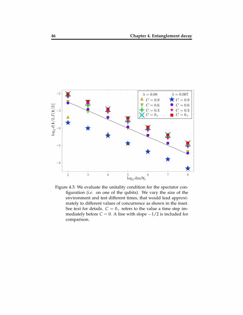
46 Chapter 4. Entanglement decay
2 3 4 5 6 7 8
-6
-5
-4
-3
-2
log 2
d(11
/2,E(
11/2)
]
log2 dimHe
λ = 0.08 λ = 0.007C = 0.9C = 0.9C = 0.6C = 0.6C = 0.3C = 0.3C = 0+C = 0+
Figure 4.3: We evaluate the unitality condition for the spectator con-figuration (i.e. on one of the qubits). We vary the size of theenvironment and test different times, that would lead approxi-mately to different values of concurrence as shown in the inset.See text for details. C = 0+ refers to the value a time step im-mediately before C = 0. A line with slope −1/2 is included forcomparison.
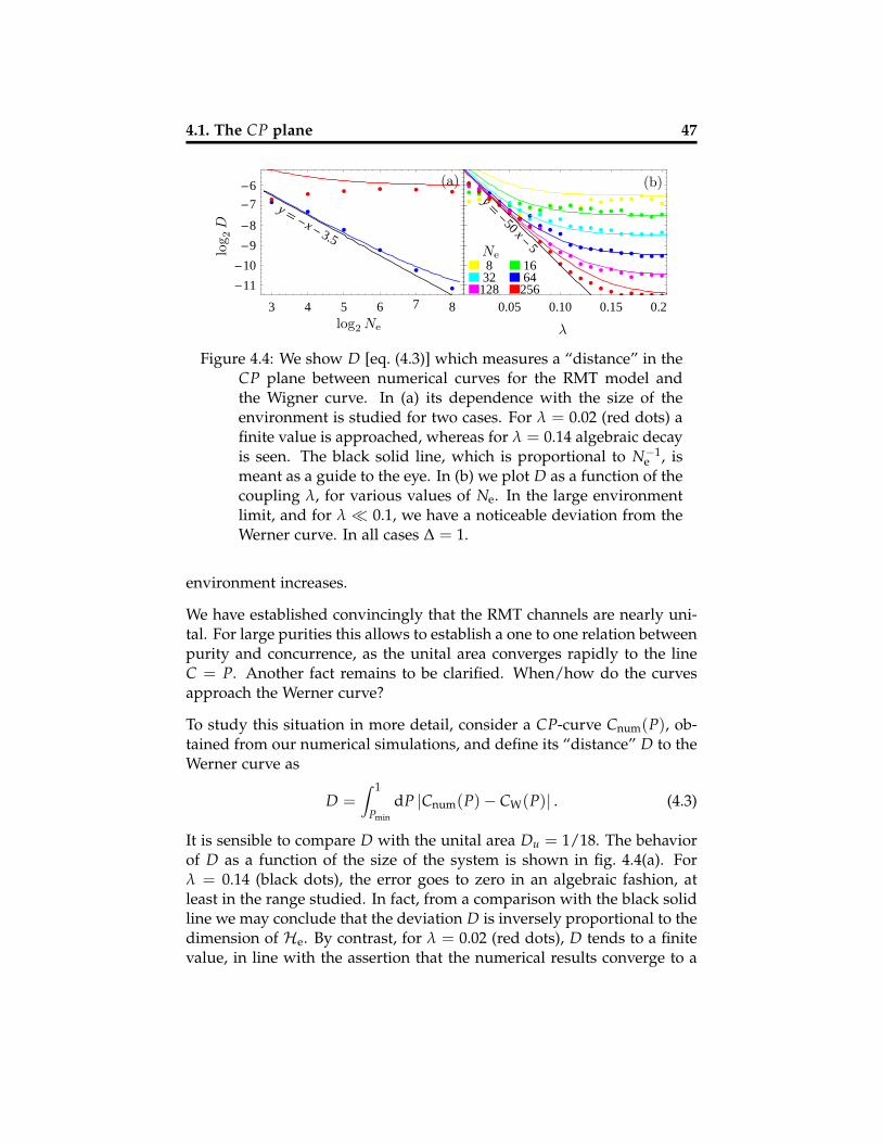
4.1. The CP plane 47
y �-x- 3.5
3 4 5 6 7 8
-11
-10
-9
-8
-7
-6
log2 Ne
log 2
D
(a)y�-50 x-
5
832128
1664256
0.05 0.10 0.15 0.20
Ne
(b)
λ
Figure 4.4: We show D [eq. (4.3)] which measures a “distance” in theCP plane between numerical curves for the RMT model andthe Wigner curve. In (a) its dependence with the size of theenvironment is studied for two cases. For λ = 0.02 (red dots) afinite value is approached, whereas for λ = 0.14 algebraic decayis seen. The black solid line, which is proportional to N−1
e , ismeant as a guide to the eye. In (b) we plot D as a function of thecoupling λ, for various values of Ne. In the large environmentlimit, and for λ � 0.1, we have a noticeable deviation from theWerner curve. In all cases ∆ = 1.
environment increases.
We have established convincingly that the RMT channels are nearly uni-tal. For large purities this allows to establish a one to one relation betweenpurity and concurrence, as the unital area converges rapidly to the lineC = P. Another fact remains to be clarified. When/how do the curvesapproach the Werner curve?
To study this situation in more detail, consider a CP-curve Cnum(P), ob-tained from our numerical simulations, and define its “distance” D to theWerner curve as
D =∫ 1
Pmin
dP |Cnum(P)− CW(P)| . (4.3)
It is sensible to compare D with the unital area Du = 1/18. The behaviorof D as a function of the size of the system is shown in fig. 4.4(a). Forλ = 0.14 (black dots), the error goes to zero in an algebraic fashion, atleast in the range studied. In fact, from a comparison with the black solidline we may conclude that the deviation D is inversely proportional to thedimension of He. By contrast, for λ = 0.02 (red dots), D tends to a finitevalue, in line with the assertion that the numerical results converge to a

48 Chapter 4. Entanglement decay
different curve. In fig. 4.4(b) we plot the error D as a function of λ, fordifferent dimensions of He. The results suggest an exponential decay ofD with the coupling strength. The simplest dependence of the deviationin agreement with these two observations is
D∆=1 =1
23.5Ne+
125+50λ
. (4.4)
We also plot the curves corresponding to this ansatz in fig. 4.4. Goodagreement is observed for D � Du. Notice the exponential decay of Dwith respect to λ. One can thus, in an excellent approximation for largeλ, say that for large dimensions the limiting curve is the Werner curve.For ∆ = 0, all studied couplings numerical convergence to the Wernercurve was observed in the large Ne limit.
In the presence of TRI the CP-curves a similar behavior is observed when-ever ∆ > 0. However, in contrast to the GUE case, no saturation of thedeviation D was observed when ∆ = 0. In the other configurations con-sidered (the joint and the separate environment), the behavior is similar.In those cases it is the largest (of the two) coupling strength which domi-nates the behavior in the CP plane (as well, naturally, as in time).
4.2 Entanglement decay
Sufficiently close to P = 1, the above arguments imply a one to one corre-spondence between purity and concurrence, which simply reads C ≈ P.This allows to write an approximate expression for the behavior of con-currence as a function of time
Clr(t) = PLR(t), (4.5)
using the appropriate linear response result for the purity decay. Thecorresponding expressions for purity decay have been discussed in de-tail in the previous chapters. Eq. (4.5) has similar limits of validity asthe linear response result for the purity. As it follows from a linear re-sponse approximation for purity, we call it a linear response expressionfor concurrence decay.
In those cases where the deviation from the Werner curve [see eq. (4.1)] issmall and where the exponentiated linear response expression eq. (2.21)holds for the average purity, we can write down a phenomenological
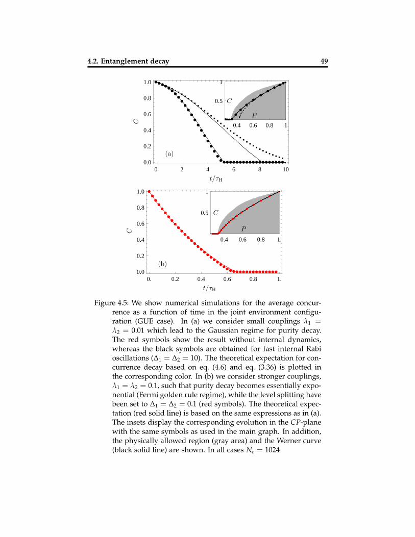
4.2. Entanglement decay 49
0.4 0.6 0.8 1
0.5
1
0 2 4 6 8 100.0
0.2
0.4
0.6
0.8
1.0
(a)
C
C
P
t/τH
0.4 0.6 0.8 1.
0.5
1
0. 0.2 0.4 0.6 0.8 1.0.0
0.2
0.4
0.6
0.8
1.0
(b)
C
C
P
t/τH
Figure 4.5: We show numerical simulations for the average concur-rence as a function of time in the joint environment configu-ration (GUE case). In (a) we consider small couplings λ1 =λ2 = 0.01 which lead to the Gaussian regime for purity decay.The red symbols show the result without internal dynamics,whereas the black symbols are obtained for fast internal Rabioscillations (∆1 = ∆2 = 10). The theoretical expectation for con-currence decay based on eq. (4.6) and eq. (3.36) is plotted inthe corresponding color. In (b) we consider stronger couplings,λ1 = λ2 = 0.1, such that purity decay becomes essentially expo-nential (Fermi golden rule regime), while the level splitting havebeen set to ∆1 = ∆2 = 0.1 (red symbols). The theoretical expec-tation (red solid line) is based on the same expressions as in (a).The insets display the corresponding evolution in the CP-planewith the same symbols as used in the main graph. In addition,the physically allowed region (gray area) and the Werner curve(black solid line) are shown. In all cases Ne = 1024
50 Chapter 4. Entanglement decay
formula for concurrence decay, which is valid over the whole range ofthe decay
Celr(t) = CW(PELR(t)) . (4.6)
In fig. 4.5 we show random matrix simulations for concurrence decay inthe joint environment configuration. We consider small couplings λ1 =λ2 = 0.01 which lead to the Gaussian regime for purity decay, as wellas strong couplings λ1 = λ2 = 0.1 which lead to the Fermi golden ruleregime. We find good agreement with the prediction of eq. (4.6), exceptfor the Gaussian regime when we switch-on a fast internal dynamics inboth qubits (∆1 = ∆2 = 10) and consequently D is large. See the insetsin fig. 4.5. Notice how in both the heuristic formula and the Monte Carlosimulations, we observe entanglement sudden death [YE04].
Note that, in the separate environment case, the entanglement of the twosubsystems defined on the spaces H1 ⊗He and H2 ⊗He′ is constant intime. For the initial conditions we use, the entanglement stems entirelyfrom the two qubits. The concurrence of these two qubits decays becausethe constant entanglement spreads over all constituents of the two largesubspaces.
We now investigated pure initial states of the qubits that are not Bellstates. Consider the GUE case with no internal Hamiltonian, in the spec-tator configuration. As discussed in previous sections, thanks to the sym-metry of the ensemble, we can write the state as
|ψ12〉 = cos θ|00〉+ sin θ|11〉. (4.7)
The initial concurrence is C0 = sin 2θ; for θ = π/4 we obtain initial Bellstates. Applying the totally depolarizing channel to one or both qubits,results in Werner states. For θ 6≡ π/4 (mod π/2), applying the channelto a single qubit or to both qubits results in different evolutions in the CPplane. Since we are considering the spectator configuration it is sensibleto apply it to a single qubit. If we parametrize the depolarizing channel[NC00] using the Kraus operators {√1− γ11,
√γ/3 σx,
√γ/3 σy,
√γ/3 σz},
we obtain the state
ρ =
13 (3− 2γ)λ 0 0 1
3 (3− 4γ)√
(1− λ)λ
0 23 γ(1− λ) 0 0
0 0 2γλ3 0
13 (3− 4γ)
√(1− λ)λ 0 0 1
3 (3− 2γ)(1− λ)
,
(4.8)

4.2. Entanglement decay 51
0.4 0.6 0.8 1.
0.2
0.6
1
a
0.3 0.4 0.5 0.6 0.7 0.8 0.9 1.00.0
0.2
0.4
0.6
0.8
1.0
C
P
2 4 6 8
0.4
0.6
0.8
1.
b
2 4 60.0
0.2
0.4
0.6
0.8
1.0
C
P
t/τH
t/τH
Figure 4.6: On the top panel the behavior in the CP plane for differentpure states is shown. We let the initial states have C = 1, 2/3, or1/3. The red curves are the ones described by the states when atotally depolarizing channel acts on the first qubit, whereas theblack dots correspond to Monte Carlo simulations. In the insetwe see theoretical curves for other initial concurrences. On thelower panel in the inset, we see the exponentiated formula forpurity decay (blue line) and the Monte Carlo averaged purity(black dots). On the main panel we see theoretical result (blueline) and 30 samples from the numerical ensemble (thin blacklines). ∆ = 0, λ = 0.01, and dimHe = 256.
52 Chapter 4. Entanglement decay
with C0 = 2√
λ(1− λ). Concurrence for this state is max{C0(1− 2γ), 0}and purity is 1 +
[4γ2(2 + C0)− 6γ(2 + C2
0)]
/9. Inverting gamma interms of purity and the initial concurrence, we can insert it in the for-mula for concurrence to obtain the Werner-like relations
CW,C0 = C0
32
√1− 4(1−P)
2+C20− 1
2 if 9P > 5− C20 ,
0 otherwise. (4.9)
The comparison between numerics and the ansatz is presented in fig. 4.6(a).The agreement is more than satisfactory. We also show in the inset a setof curves for more values of C0. The success of the description allowsto give a heuristic concurrence decay formula for initial states, not beingBell states along the same lines as in the previous paragraphs and usingeq. (4.9) instead of eq. (4.1). A comparison between our heuristic formulaand Monte Carlo simulation is presented in fig. 4.6(b). Note that ”suddendeath” of entanglement [YE04] persists, though it happens at differentpurities. This is also visible for the individual members of the ensemble.
CW,C0 = max
0,C0 − 1
3+
1 + 2C0
3Re−1 +
√1− (1 + C2
0)(3− 6P− C20)
1 + C20
(4.10)
is the analogous expression for concurrence in terms of purity, when bothqubits are coupled with similar strength.
Chapter 5
An example, the KI chain
5.1 Introduction
In this chapter we continue studying decoherence and entanglement de-cay using two qubits as the central system. We pursue two main ob-jectives. The first one is to test some of the qualitative and quantitativeconclusions we have derived in the previous chapters, in a deterministicmodel. The second one is to explore dynamical regimes that, up to thispoint, we have ignored: integrable dynamics and intermediate dynamics(not integrable but with chaos not fully developed). We shall focus onthree points. First we wish to study how dynamics of the environment,i.e. its integrability or chaoticity influence the behavior of decoherenceand internal entanglement. Second, we shall analyze to what extent pu-rity and concurrence may be related. In particular we want to test thereach of the relation discovered in sec. 4. Finally, we wish to relate quan-titatively the behavior of purity, in the chaotic regime, with the resultsobtained with RMT in the previous chapters. To implement such a pro-gram we need a model with flexible dynamics, which allows efficientnumerics for large Hilbert spaces.
The fact that the central system consists of two qubits, makes a spin sys-tem an attractive candidate. Indeed the kicked Ising spin chain, a modelintroduced by Prosen [Pro02], was used to study decay of fidelity and pu-rity [PS02] in echo dynamics for integrable, chaotic (more precisely mix-ing [Pro00]) as well as for intermediate cases. Results for purity in echodynamics can be used for purity decay in standard forward dynamics if
53
54 Chapter 5. An example, the KI chain
the perturbation is chosen as the coupling between the central system andthe environment, sec. 2.2. The main advantage of this model is the highcomputational efficiency that allows to perform numerical calculationsup to twenty qubits [PSPS06] and more on any good workstation. Yet themodel in its original form does not allow for variable Ising interactions,and is thus not well suited outside of the field of echo dynamics. Exper-imental realizations of similar models have been proposed [BMM05] andrelated studies appeared in [LS05].
In the present chapter we shall generalize this model allowing arbitraryinteractions between the spins, and site dependent kicks (this does not af-fect the numerical efficiency of the model, see appendix B). We then usethe generalized model to study the evolution of purity and concurrence ofcentral system (consisting of two spins) initially in a Bell state, evolving inenvironments with different dynamical properties. As we want concur-rence to be affected solely by the coupling to the environment, we choosenon-interacting spins for the selected pair. Some preliminary results werepublished in [PS06]. For the environment it is sensible to consider ran-dom states to emulate a bath at fairly high temperature. Using unitarytime evolution of the total system and partial tracing over the environ-ment we can then calculate concurrence and purity decay of the selectedpair, and discuss their behavior.
To discuss the general model we first recall and discuss a particular caseof the model which, in fact, will help to understand the properties of theenvironment (sec. 5.2). Then we state the general model and discuss theparticular configurations to be studied (sec. 5.3). Next we proceed to dis-cuss the behavior in time of both concurrence and purity for the differentconfigurations and different dynamics, sec. 5.4. Afterwards, in sec. 5.5,we discuss the relation between concurrence and purity. Finally, we com-pare purity evolution with the corresponding RMT model in sec. 5.6.
This chapter is largely based on [PS06]; however, we have learned a lotsince its publication. Further research and major rewriting were thus re-quired to contextualize and discuss the results presented here. We addednew configurations and discuss in detail the physical differences betweenthe different models. The comparison with RMT is now possible as thetheory is completed.
5.2. The kicked Ising spin chain 55
5.2 The kicked Ising spin chain
We first study the kicked Ising chain (KIC) [Pro02]: A ring of L spin 1/2particles which interact with their nearest neighbors via a homogeneousIsing interaction of dimensionless strength J, and are periodically kickedwith a dimensionless homogeneous magnetic field ~b.The Hamiltonian isthus
H = JL
∑j=1
σzj σz
j+1 + δ1(t)L
∑j=1
~b ·~σj (5.1)
where δ1(t) = ∑n∈Z δ(t − n) represents an infinite train of Dirac deltafunctions with primitive period one; σ
x,y,zj are the Pauli matrices of par-
ticle j and ~σj = (σxj , σ
yj , σz
j ). We must also impose periodic conditions inorder to close the ring: ~σL+1 ≡~σ1. During the free evolution, i.e. betweenthe kicks, the system evolves with the unitary propagator
UIsing(J) = exp
(−iJ
L
∑j=1
σzj σz
j+1
), (5.2)
and the action of the kick is described by the unitary operator
Ukick(~b) = exp
(−i
L
∑j=1
~b ·~σj
). (5.3)
The Floquet operator for one period is thus
UKI = UIsing(J)Ukick(~b). (5.4)
A detailed discussion of the symmetries of the system can be found in[PP07]. We summarize the main observations here. Due to the homo-geneity of the kick ~b and the nearest neighbor interaction J, the systemhas a rotational symmetry~σj →~σj+1. The dimension of each of the invari-ant subspaces (Hk with k = 1, . . . , L) is close to 2L/L for large L. Each ofthe invariant subspaces has an anti-unitary symmetry which, if we choosea base in which~b ·~σj is real, is complex conjugation (i.e. not conventionaltime reversal symmetry). Since each minimal invariant subspace has aninternal anti-unitary symmetry, it is reasonable to compare with the GOEor the COE to understand the properties of the system.
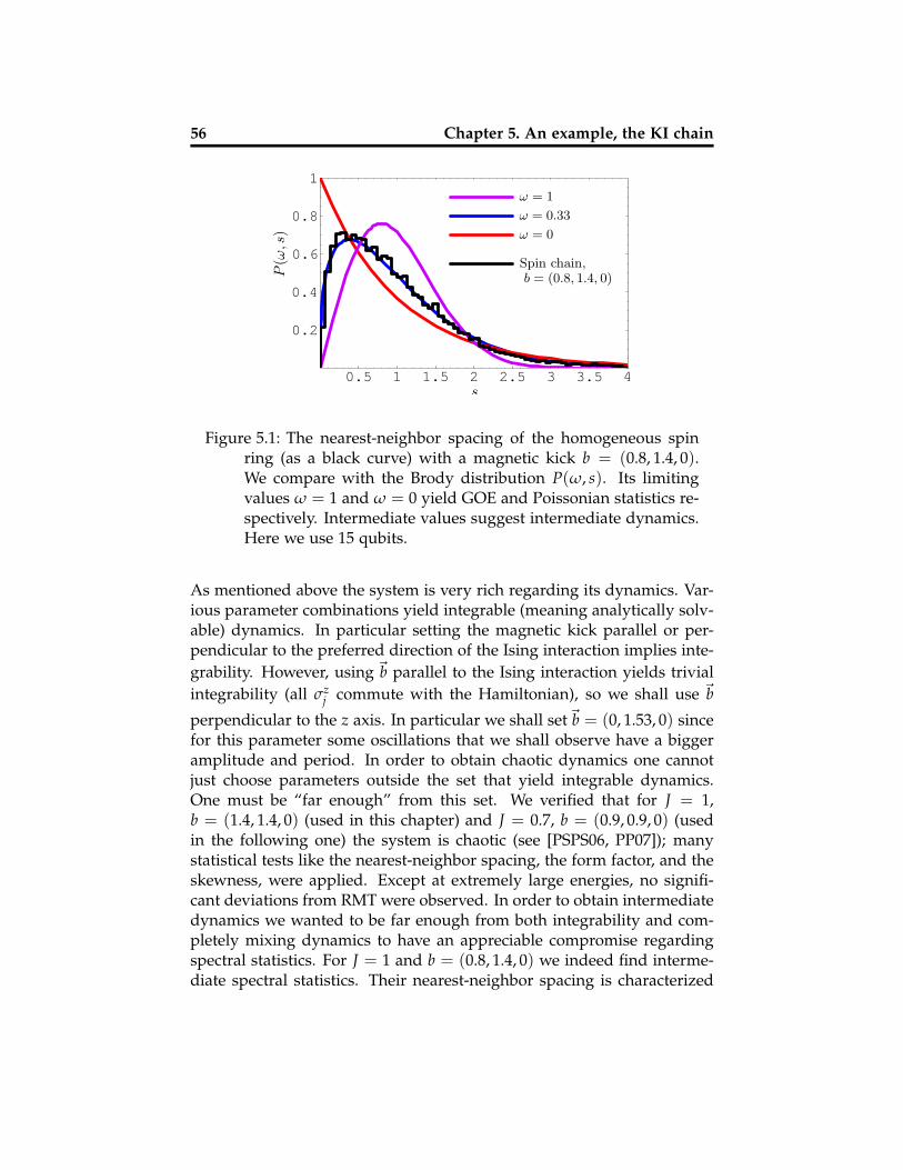
56 Chapter 5. An example, the KI chain
0.5 1 1.5 2 2.5 3 3.5 4
0.2
0.4
0.6
0.8
1
P(ω
,s)
s
ω = 0
ω = 0.33
ω = 1
Spin chain,b = (0.8, 1.4, 0)
Figure 5.1: The nearest-neighbor spacing of the homogeneous spinring (as a black curve) with a magnetic kick b = (0.8, 1.4, 0).We compare with the Brody distribution P(ω, s). Its limitingvalues ω = 1 and ω = 0 yield GOE and Poissonian statistics re-spectively. Intermediate values suggest intermediate dynamics.Here we use 15 qubits.
As mentioned above the system is very rich regarding its dynamics. Var-ious parameter combinations yield integrable (meaning analytically solv-able) dynamics. In particular setting the magnetic kick parallel or per-pendicular to the preferred direction of the Ising interaction implies inte-grability. However, using ~b parallel to the Ising interaction yields trivialintegrability (all σz
j commute with the Hamiltonian), so we shall use ~b
perpendicular to the z axis. In particular we shall set~b = (0, 1.53, 0) sincefor this parameter some oscillations that we shall observe have a biggeramplitude and period. In order to obtain chaotic dynamics one cannotjust choose parameters outside the set that yield integrable dynamics.One must be “far enough” from this set. We verified that for J = 1,b = (1.4, 1.4, 0) (used in this chapter) and J = 0.7, b = (0.9, 0.9, 0) (usedin the following one) the system is chaotic (see [PSPS06, PP07]); manystatistical tests like the nearest-neighbor spacing, the form factor, and theskewness, were applied. Except at extremely large energies, no signifi-cant deviations from RMT were observed. In order to obtain intermediatedynamics we wanted to be far enough from both integrability and com-pletely mixing dynamics to have an appreciable compromise regardingspectral statistics. For J = 1 and b = (0.8, 1.4, 0) we indeed find interme-diate spectral statistics. Their nearest-neighbor spacing is characterized

5.3. A generalized kicked Ising model 57
by a Brody parameter [Bro73] of 0.33, see fig. 5.1. The nearest-neighborspacing distribution in the Floquet spectrum shows a marked level repul-sion, but it is still quite far from the distribution we expect and get forthe chaotic case.
5.3 A generalized kicked Ising model
The Hamiltonian of the generalized kicked Ising model is
H =L
∑j>k=1
Jj,kσzj σz
k + δ1(t)L
∑j=1
~bj ·~σj. (5.5)
The model thus consists of a set of L spin 1/2 particles coupled to allother spins by an Ising interaction (first term) and periodically kicked bya site dependent tilted magnetic field (second term).
Our model differs from the one stated in eq. (5.1) by the fact that the cou-pling Jj,k is between any pair of particles and has an arbitrary strength.This freedom allows to build a variety of models with different topolo-gies. Each of them will correspond to a well defined physical picture, andthus we show how the flexibility of the model can be exploited to studydiverse physical situations in a common framework. We also allow siteindependent kicks to be able to have (or not) internal dynamics in ourcentral system.
The central system is composed of two spins, say spins “1” and “2”.We are left with qe = L − 2 spins which are going to be considered asthe environment. We furthermore diminish the number of parametersby setting ~b1 = ~b2 = ~bc and ~b3 = · · · = ~bL = ~be. The fact that wekeep the kick in the central system can represent local operations madeby the “owners” of each of the qubits, and will not affect the values ofconcurrence and purity. We shall furthermore require weak coupling ofthe central system to the environment. Thus Ji,1 and Ji,2 must be muchsmaller than the typical Ising interaction within the environment. Weset J2,1 = 0 in order to prevent any interaction between the spins in thecentral system.
We propose in particular six models. They are schematically drawn infig. 5.2. The open circles represent qubits 1 and 2 (the central system)whereas the filled circles represent the other qubits (environment). The

58 Chapter 5. An example, the KI chain
(a) (b) (c)
(d) (e) (f)
Figure 5.2: Different configurations of the coupling of the central sys-tem (represented as open circles) to the spins that act as envi-ronment (represented as filled circles). Thick/thin lines repre-sent J′ce/Je respectively. The description for each model and itsfeatures is given in the main text.
thin lines represent a weak Ising interaction J′ce of a particle in the centralsystem with one in the environment. The thick lines represent an interac-tion Je among particles in the bath; in all numerical results presented wefix Je = 1. Finally we note that the dimension of the Hilbert space of theenvironment is Ne = 2qe . Writing the Hamiltonian for each of the modelswe propose is now a trivial task. As an example we write the Hamilto-nian of the model (a) in fig. 5.2: Rewriting the Hamiltonian in terms ofcentral system, environment and interaction as H = Hc + He + Hce theparts are given by
Hc = δ1(t)2
∑j=1
~bc ·~σj, (5.6)
He = Je
L−1
∑j=3
σzj σz
j+1 + δ1(t)L
∑j=3
~be ·~σj (5.7)
Hce = J′ceσz2 σz
3 . (5.8)
Each of the models has a characteristic Heisenberg time τH. For a sys-tem with no symmetries the Heisenberg time is defined simply as 2π/d,where d is the mean level spacing. If the system has symmetries, foreach sector we have a Heisenberg time defined again as 2π/d, but d isthe mean level spacing in each sector. We shall stress the Heisenbergtime of each model, as our RMT models show a strong dependence onit [e. g. eq. (3.23)]. We also use a normalized coupling Jce, which givesa model independent coupling strength. Finally, we want to mention the

5.3. A generalized kicked Ising model 59
corresponding configuration (spectator, joint environment or separate en-vironment), as in sec. 3.1.
Please refer to fig. 5.2 while reading the descriptions.
• Model (a) is in the spectator configuration. A single qubit is cou-pled to the extreme of an open chain. Due to the breaking of thesymmetry of the coupling, the Heisenberg time of the environmentis τH ≈ Ne. We use the normalized coupling Jce = J′ce.
• The second model is a variation of the previous one. In this thesecond qubit is coupled to the other extreme of the chain. It is anexample of the joint environment configuration. Again τH ≈ Ne,however to have the same effective coupling we must scale Jce =√
2J′ce.
• Model (c) is the last of this family of models in which the environ-ment is an open chain. In this case τH ≈
√Ne � Ne. As we have
two coupling spots, we must scale Jce =√
2J′ce. This is a good exam-ple of a separate environment Hamiltonian. This, and the previoustwo models, were analyzed in [PS06].
• Model (d) is again in the spectator configuration, but here we havea ring (thus the translational symmetry is not broken) and the cou-pling is symmetric. The Heisenberg time is then related to eachsymmetry sector separately and is approximately equal to Ne/qe.The coupling must be normalized to Jce = √qe J′ce.
• The next model differs from the previous one only inasmuch thatthe coupling is not symmetric. This is enough to mix the invariantsubspaces and thus the Heisenberg time is ≈ Ne. There is a singlecoupling and thus it is enough to set Jce = J′ce.
• Model (f) is another example of a separate environment config-uration. It has the smallest Heisenberg time, since the couplingdoes not break the symmetry of the ring. Thus, it is approximately√
Ne/qe. The coupling is normalized to Jce = √qe J′ce.
It is pertinent to mention, that the degree of chaoticity was obtained forcyclic chains, while the chains representing some of our environments areopen. Yet, for large number of spins, this is irrelevant.

60 Chapter 5. An example, the KI chain
The non-unitary evolution of the central system alone is calculated alongthe same lines as for the RMT models. We perform a unitary evolutionof the whole system (yielding state |ψ(t)〉) and then we partial trace overthe environment. That is
ρ(t) = tre |ψ(t)〉〈ψ(t)|. (5.9)
We shall consider an initial condition
|ψ(t = 0)〉 = |ψBell〉 ⊗ |ψenv〉, (5.10)
i.e. a general Bell state [any state such that C(|ψBell〉〈ψBell|) = 1] notentangled with the environment, which is in a pure random state [formodels (a), (b), (d), and (e)] or in a tensor product of pure random statesin each section of the environment [for models (c) and (f)].
5.4 The evolution of concurrence and purity
We now present the results of our numerical calculations of both concur-rence and purity of the selected pair of spins as a function of time. Wefirst concentrate on the short time behavior.
Fig. 5.3 shows the time evolution of purity of the selected pair of spins forthe initial state consisting of a Bell pair in the central system and the ap-propriate random state in the environment. We choose the environmentto be chaotic in one case and integrable in the other, using the correspond-ing parameters mentioned in sec. 5.2. The chaotic environment leads tolinear decay for some time interval, while the integrable environmentleads to a quadratic decay. The interval in which the linear decay can beobserved depends on two things: the configuration and the dimensionof the environment. Indeed, for configuration (f) we have the shortestlinear decay but we also have the shortest Heisenberg time. The readeris encouraged to check table 5.4 to understand better our numerical re-sults. Recall that in all our derived formulae, we predicted linear decaybefore Heisenberg time. The situation for the integrable case is different.We observed a marked quadratic decay, independent of the configurationand the size of the environment. We believe that one should be able toexplain the results (for the integrable situation) with exact analytic cal-culations, however the aim of this chapter is not to explain the details,but to illustrate the qualitative differences between having a chaotic andregular environment.
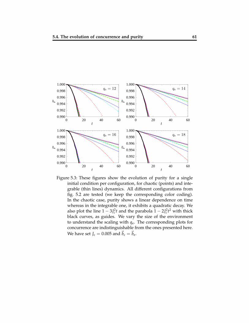
5.4. The evolution of concurrence and purity 61
0 20 40 600.990
0.992
0.994
0.996
0.998
1.000
P
t
qe = 12
0 20 40 600.990
0.992
0.994
0.996
0.998
1.000
Pt
qe = 14
0 20 40 600.990
0.992
0.994
0.996
0.998
1.000
P
t
qe = 16
0 20 40 600.990
0.992
0.994
0.996
0.998
1.000
P
t
qe = 18
Figure 5.3: These figures show the evolution of purity for a singleinitial condition per configuration, for chaotic (points) and inte-grable (thin lines) dynamics. All different configurations fromfig. 5.2 are tested (we keep the corresponding color coding).In the chaotic case, purity shows a linear dependence on timewhereas in the integrable one, it exhibits a quadratic decay. Wealso plot the line 1− 3J2
c t and the parabola 1− 2J2c t2 with thick
black curves, as guides. We vary the size of the environmentto understand the scaling with qe. The corresponding plots forconcurrence are indistinguishable from the ones presented here.We have set Jc = 0.005 and~bc =~be.

62 Chapter 5. An example, the KI chain
(a) � (b) � (c) � (d) � (e) � (f) �qe = 12 4096 4096 64 341.3 4096 10.7qe = 14 16348 16348 128 1170.3 16348 18.3qe = 16 65536 65536 256 4096 65536 32qe = 18 262144 262144 512 14563 262144 56.9
Table 5.1: Numerical values of the Heisenberg times for the differentconfigurations of the environment, and different sizes of it.
We now proceed to look at the long-time evolution of concurrence andpurity again for all configurations. In Fig. 5.4 we show both concurrenceand purity for integrable, intermediate and chaotic situations.
For the integrable case we see that for some configurations [(a), (b), and(c)] after the initial quadratic decay there is a full revival of both concur-rence and purity. However the autocorrelation function of the full system(not shown) drops fast and reaches negligible values even after the firstfew kicks. It is also worthwhile to note that the oscillations of purityimply increase in some cross-correlation function [PSZ03]. For the otherconfigurations there is no such revival, and the decay seems Gaussian;this is in agreement with the quadratic decay observed for large purities.Notice that in all the configurations in which there is a revival the cou-pling is to one end of a chain. Notice how concurrence drops to exactly 0after a finite time.
For the chaotic case we observe a monotonic decay of both purity andconcurrence. The speed at which they decay, though initially the same,is quite different for the different configurations. This can be explainedwith the huge differences in the Heisenberg times of the environment.
For the mixed case, we observe a compromise among the behavior in theintegrable case and the chaotic one. Interestingly in all cases we observedthat concurrence drops identically to zero after some time, in contrastwith purity which does no reach its minimum.

5.5. A relation between concurrence and purity 63
Chaotic
Mixed
Integrable
0 200 400 600 0 200 400 600 8000.
0.20.40.60.80.
0.20.40.60.80.
0.20.40.60.81.
0.0.20.40.60.80.0.20.40.60.80.0.20.40.60.81.
t
P C
Figure 5.4: Long-time behavior of purity (left) and concurrence(right) for an arbitrary initial condition in integrable (top), non-ergodic and non-integrable (middle), and fully chaotic (bottom)regimes. For the integrable regimes we observe recurrences forthe open environment configurations and fast, possibly Gaus-sian, decay in the others. For the intermediate case we observein some instances the superposition of oscillations together withthe exponential decay. For the chaotic case we observe expo-nential decay together with a marked dependence on the kindof environment. We have set qe = 16, Jc = 0.02, and~bc =~be.
5.5 A relation between concurrence and purity
The rather similar pictures emerging for concurrence and purity suggestthat a simple relation between the two might emerge. Indeed, from theresults of the previous chapter this could be expected for the chaotic case.Unfortunately we are not able to access such a big range of values of thecoupling as in the previous section; too strong coupling leads to total con-currence decay after a single period (remember that we are dealing withFloquet operators). Too weak couplings imply too long runs as we have tointegrate one step at a time. On the other hand, we are going to be able totest the relation not only on chaotic situations but also in other dynamicalregimes such as integrable environments and intermediate environments.
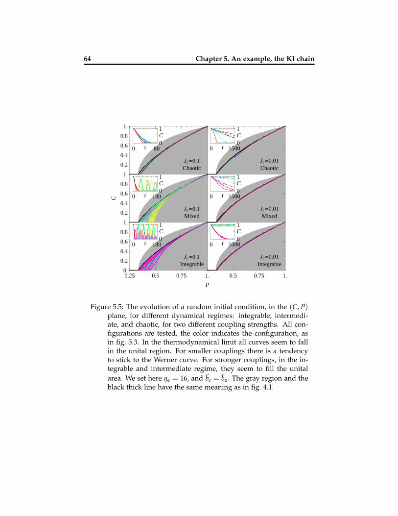
64 Chapter 5. An example, the KI chain
0 t 1800C1
0 t 1800C1
0 t 800C1
0 t 10000C1
0 t 15000C1
0 t 15000C1
IntegrableJc=0.1
IntegrableJc=0.01
MixedJc=0.1
MixedJc=0.01
ChaoticJc=0.1
ChaoticJc=0.01
0.25 0.5 0.75 1. 0.5 0.75 1.0.
0.2
0.4
0.6
0.8
1.
0.2
0.4
0.6
0.8
1.
0.2
0.4
0.6
0.8
1.
P
C
Figure 5.5: The evolution of a random initial condition, in the (C, P)plane, for different dynamical regimes: integrable, intermedi-ate, and chaotic, for two different coupling strengths. All con-figurations are tested, the color indicates the configuration, asin fig. 5.3. In the thermodynamical limit all curves seem to fallin the unital region. For smaller couplings there is a tendencyto stick to the Werner curve. For stronger couplings, in the in-tegrable and intermediate regime, they seem to fill the unitalarea. We set here qe = 16, and~bc =~be. The gray region and theblack thick line have the same meaning as in fig. 4.1.
5.5. A relation between concurrence and purity 65
We plot in fig. 5.5 concurrence against purity in all the dynamical regimesstudied so far. We do so for two strengths of the perturbation, namelyJc = 0.1 and 0.01. A wide variety of behaviors are observed. One thingthat stands out is that all curves lie in the unital region. Indeed for J =0.1, in the integrable and intermediate regime we observe a filling of theunital region [recall it from fig. 4.1]. This is not a finite dimension effect:we verified that the behavior remains for increasing dimension of theenvironment in both cases. For small dimensions, and in configuration(b) one observes that the curves do not lie in the unital region and explorea larger area. This can be explained: one has a common environmentwhich, in fact, has memory (due to its small dimension). An example ofthis behavior can be found in figure 5 of [PS06].
For the other cases, where there is no filling of the unital region, one cansuspect self averaging. This can be tested calculating the standard de-viation of purity σP , one time step before concurrence is zero. This isequivalent to examining the width of the coloured curves in fig. 4.1. Wenumerically observed that for some set of parameters, σP ∝ 1/Ne whereasfor other it approaches a finite value. Though a tendency to accumulatetowards the Werner curve is clear from the pictures presented, in somecases it is not more than a tendency. Indeed, even in the chaotic case andwhen having self averaging, the limiting curve not always crosses the lineC = 0 at P = 1/3 (like the Werner curve), but a slighter bigger value.Again our numerics show that this is not a finite size effect. However, allthe limiting curves are similar to the Werner curve, and that still can beused for approximations, as long as we recall it is only an approximation.Though all six configurations are physically quite different and the indi-vidual behavior of purity and concurrence is quite affected, the relationbetween the two is entirely robust.
Cases (c) and (f) lead to an instructive lesson: Here we have two uncou-pled environments, and we start with a pure state in each of these. Thepurity of the uncoupled subsystems will remain unchanged, but the pu-rity and concurrence of the initial Bell pair will decay. Thus one mightconsider seeing a paradox, but this is not the case; the entanglement ofthe pair is simply spread over all the system with time.
Up to this point our results are in full qualitative agreement with the onesfound in previous chapters. This leads us to make a tighter comparisonwith the RMT models developed before.

66 Chapter 5. An example, the KI chain
5.6 Comparison with RMT predicted behavior
Our KI model has some parameter ranges in which we can consider thesystem to be “quantum chaotic”. A quantitative comparison of puritydecay for the dynamical system and the RMT model is sound. Statisticaltests and analytical arguments, indicate that one can consider the homo-geneous KI as a typical member of the GOE. Thus we shall compare withthe results obtained in sec. 2.5 and sec. 3.2.2. We first list some differencesbetween the two models.
• The most serious difference is the structure of the coupling. Relationsof the form eqs. (E.4) and (E.5) used to define the coupling in the RMTmodel, generically yield non-separable operators, whereas the couplingfor the KI model is indeed separable and of the form σz ⊗ Ve. Dynamicsinvolving separable operators have special properties. We must not besurprised that this particular structure of the coupling affects the behav-ior.
• The theory developed in earlier chapters is for an ensemble of systems.Here we are dealing with a single system. Self averaging takes care ofthis issue. Numerical tests indicate that as the size of the environmentincreases, the behavior for a typical Hamiltonian approaches rapidly thebehavior of the ensemble average (see fig. 2.3). We can safely ignorethis problem as long as we go to high enough dimensions. However,for very detailed discussions this must be taken into consideration (as in[PSPS06]).
•We are using environments with either exact rotational symmetries [(d),(e), and (f)] or with some approximate translational symmetry [(a), (b),and (c)]. But we have not developed a theory for chaotic environmentswith discrete unitary symmetries.
One might be tempted to assume that the overall result is an average ofthe results in the different sectors, as happens with fidelity f : Given anecho operator M with a discrete unitary symmetry, and a set of states{|ψs〉} living in the different symmetry sectors,
f = (∑s
α∗s 〈ψs|)M(∑s′
αs′ |ψs′〉) = ∑s|αs|2〈ψs|M|ψs〉.

5.6. Comparison with RMT predicted behavior 67
For purity the situation is different,
P
(tr1 ∑
s,s′αsαs′ |ψs〉〈ψs′ |
)6= ∑
s|αs|2P(tr1 |ψs〉〈ψs|). (5.11)
Let α1 = α2 = 1/√
2, |ψs=1〉 = |00〉, and |ψs=2〉 = |11〉. In this case purityof the reduced system is minimal (1/2) whereas the purity of the reducedstate of each of the components is maximal (1).
However, a quantity that is affected immediately when superposing spec-tra is the form factor. The form factor of a superposition of many, sayGOE, spectra approaches that of a Poissonian one. Thus, a simplifiedway to incorporate this effect is to replace in our formulae the GOE formfactor b(1)
2 (t) by the one of a random spectra b2(t) = 0.
• During the first chapters we assumed time independent Hamiltonians.The KI Hamiltonian (5.5) depends explicitly on time. However, due toits periodic nature, one can construct its corresponding Floquet opera-tor. The circular ensembles [Dys62] are used to model such operators[Haa01]. Circular and Gaussian ensembles share all the properties re-garding its eigenvectors. The eigenphases of the former and the eigenval-ues of the later share most properties but a precise mathematical relationamong them is cumbersome to state. We can naively consider the circularensembles as an exponentiated (and approximated) version of the Gaus-sian ensembles. We thus do not need to modify our theory to take intoaccount this issue.
• With eq. (E.4) we are assuming certain normalization of the coupling.One can adjust the coupling constant λ so any V has the given normal-ization [see eq. (2.5)]. In our case, we can expect that for models (a) and(e) the decay, at least for short times, does not depend on the numberof qubits. This can be achieved substituting λ → αJce/
√τH with α an
Ne independent number. The leading term (with respect to time) is nowindependent of τH and Ne.
For simplicity we eliminate the internal Hamiltonian in the dynamicalmodel (Hc = 0) to use the RMT formulae with ∆ = 0. We use config-uration (d) for the comparison to eliminate possible border effects. ItsHeisenberg time is moderately small and thus we can access easily timeregimes comparable with the Heisenberg time. The effective size of theenvironment is still large (2qe) [compared with separate environment con-figurations (
√2qe)] so the large dimension limit is achieved faster.

68 Chapter 5. An example, the KI chain
Figure 5.6: We plot, with blue thin lines, the evolution of purity for10 initial condition in model (d). We vary the number of qubitsvertically and the time ranges horizontally. The formula de-rived from our RMT model eq. (5.12) is plotted as a thin blackline. The same formula, but assuming no correlations withinthe spectra, is plotted as a dashed line. We use J′ce = 0.0005to be in the linear response regime for all plots. See text for acomplete description.
Our adapted RMT formula (using Bell states as initial conditions) reads
P(t) = 1− α
(J′ce√
qe
)2{3tτH +
4τH
t2 − 3τH
B(1)2 (t)
}. (5.12)
The numerical results are summarized in fig. 5.6. There we find 9 plotsfor the evolution of purity in the KI chain. Each blue line corresponds to adifferent realization of the initial condition eq. (5.10). We include formula(5.12) with and without the correlation term 3
τHB(1)
2 (t) as solid and dashedblack lines respectively. We increase the size of the environment (frombottom to top)to appreciate how the large dimension limit is approached.

5.6. Comparison with RMT predicted behavior 69
We also vary the plot range to examine different time regimes of theproblem. In the plots, two time scales are available. The lower scale is thenumber of time steps (number of applications of the Floquet operator)while the upper one is time in units of the Heisenberg time.
We first encounter the Zeno regime, in which the discreteness of the spec-trum induces deviations of the RMT formulae; for a finite spectrum, whatwe take as a δ function in eq. (2.13), has a finite width and height, caus-ing an initial quadratic decay. Indeed we can see on the left most plotsthat the deviation lasts a few kicks. The effect is more visible for qe = 12and 14. The next regime is the linear one, sometimes called Fermi goldenrule regime. We observe linear decay as predicted by RMT whenever1� t � τH. We use this regime to obtain the fitting parameter α = 0.21.Next we observe a crossover in which deviations from the linear behav-ior are evident (starting at t ≈ τH/4). For qe = 10 this regime overlapsslightly with the Zeno regime. After the crossover we find the Gaussianregime, in which a quadratic decay of purity is manifest. The clearestpicture of this behavior is seen for qe = 10 where the Heisenberg time isthe smallest.
As we increase the size of the environment we observe better agreementbetween the dynamical model and the RMT formula with no correlation.For qe = 14 the agreement is virtually perfect for all time regimes beyondthe Zeno regime. Comparing the behavior for different environments, wecan observe the dramatic effect of the Heisenberg time on decoherence:The denser the spectrum, the later we arrive to the Gaussian regime. En-vironments with tighter spectra cause less damage to the central system.Other configurations also show qualitative agreement with the RMT for-mula developed before.
The results of sec. 2.5 predict that for arbitrary separable conditions, ona TRI system (or with any other anti-unitary symmetry), we have a fi-nite spreading of purity, even in the large dimension limit. This effectbecomes important after the Heisenberg time. We argued why we expectself averaging (with respect to the initial conditions) for Bell states andindeed observed it in the large dimension limit.
We tested these two findings in our KI models. As expected, we found noself averaging for separable ones. However, we observed the same effectbefore and after the Heisenberg time. This anomaly can be due to theseparable structure of the coupling, which implies a preferred base withinthe central system. From that point of view, this irregularity is analogous

70 Chapter 5. An example, the KI chain
0.1 0.2
0.999
0.9995
0 200 400 600 800 10000.94
0.95
0.96
0.97
0.98
0.99
1.001 2 3
t/τH
t
P
0.1 0.2
0.999
0.998
0 200 400 600 800 1000
0.90
0.92
0.94
0.96
0.98
1.001 2 3
t/τH
t
P
Figure 5.7: Evolution of 25 random initial conditions for configura-tion (d). In the top panel we prepare separable initial condi-tions, whereas in the lower panel entangled ones. We observeno self-averaging both for long times and short times (in theinsets). This might be due to the separable structure of the cou-pling. Jce = 0.0005 and qe = 12.
to the effect of an internal Hamiltonian. Interestingly, we again observethat for entangled states we do have self averaging. This suggests that the“transport” of symmetries via entanglement is a general property that isnot limited to the topics discussed during this thesis.

Chapter 6
Quantum memories
Divide et impera.
Physical devices capable of storing faithfully a quantum state, i.e. quan-tum memories, are crucial for any quantum information task. While dif-ferent types of systems have been considered, most of the effort is concen-trated in manipulating qubits as they are essential for most quantum in-formation tasks [NC00]. For a general quantum memory (QM) it is neces-sary to record, store, and retrieve an arbitrary state. For quantum commu-nication and quantum computation initialization in the base state, singlequbit manipulations, a two qubit gate (e.g. control-not), and single qubitmeasurements are sufficient. For arbitrary quantum memories recordingand retrieving the state is still an experimental challenge but initializinga qubit register and individual measurement is mostly mastered. Faithfulrealization of two qubit gates together with better isolation from the envi-ronment are the remaining obstacles for achieving fully operational quan-tum technology. However the huge effort done in the community hasborn some fruit [JSC+04, CdRF+05, CMJ+05, EAM+05, PF02, PFL+04].
Understanding decoherence of one, two, and n qubits has been of interestfor some time. In [FFP04] the authors calculate decoherence of a QMfor a spin-boson model using a measure designed for their purposes.In the limit of slight decoherence they obtain various results includingadditivity. Experimental results are also available [KS04, KS06]. In theprevious chapters we have studied one and two qubit decoherence usingboth a random matrix formulation and a specific dynamical model. Onewould wish to encompass some of this progress in a general picture.
71
72 Chapter 6. Quantum memories
In the present chapter we address this problem using a standard mea-sure of decoherence, namely purity. We obtain analytic expressions forthe decoherence of a QM during the storage time. Specifically we dis-cuss a QM composed of a set of individual qubits interacting with someenvironment. The expressions given are based on previous knowledgeof the decoherence of a single qubit entangled with some non-interactingspectator. Their validity is limited to small decoherence, i.e. large pu-rity of the QM. Note that the latter is not a significant restriction, withinthe context of quantum information processing, due to the high fidelityrequirements of quantum error correction codes. We again assume thatthe entire system is subject to unitary time-evolution, and that decoher-ence comes about by entanglement between the central system (CS) andthe environment. Spurious interactions inside the central system are ne-glected.
A further and critical assumption is the independence of the couplingof different qubits with the environment in the interaction picture. This isjustified if the couplings are already independent in the Schrodinger pic-ture or if we have rapidly decaying correlations due to mixing propertiesof the environment [PS02]. Physically, the first would be more likely ifwe talk about qubits realized in different systems or degrees of freedom,while the second seems plausible for many typical environments.
The central result is a decomposition of the decoherence of the full QM,coupled to a single or several environments into a sum of terms. Eachof these describes the decoherence of a single qubit in a “spectator con-figuration” eq. (1.2). Recall, the CS consists of two non-interacting parts,one (the qubit) interacting with the environment and the other (the restof the QM) not. This configuration is non-trivial if the two parts of theCS are entangled. Apart from the above assumptions, this result does notdepend on any particular property of the environment or coupling. Thus,it can be applied to a variety of models.
The general relation is obtained in linear response approximation andleads to explicit analytic results if the spectral correlations of the envi-ronment are known, see sec. 6.1. We test successfully the results in ourrandom matrix model (sec. 6.2). Finally, we perform numerical simula-tions for four qubits, interacting with the kicked Ising spin chain as anenvironment, in sec. 6.3.

6.1. The calculation 73
6.1 The calculation
We now outline the calculation for n qubits. Since it just represents avariation in the indices of some calculations presented in appendix A, weskip some details and go through it pretty fast.
The central system (our QM) is composed of n qubits. Thus, its Hilbertspace is Hqm =
⊗ni=1Hi, where Hi are the Hilbert spaces of the qubits.
The Hilbert space of the environment is again denoted byHe. The Hamil-tonian reads
H = Hqm + He + λV, λV =n
∑i=1
λiV(i). (6.1)
Here, Hqm = ∑ni=1 Hi, where Hi acts on Hi, whereas He describes the
dynamics of the environment, and λV the coupling of the qubits to theenvironment. The strength of the coupling of qubit i is controlled bythe parameter λi, while λ = max{|λi|}. The (possibly time-dependent)Hamiltonian gives rise to the unitary evolution operator Uλ(t).
We consider two different settings. In the first one V(i) acts on the spaceHi ⊗ He, i.e. all qubits interact with a single environment called jointenvironment. In the second one each qubit interacts with a separate envi-ronment. Thus the environment is split into n parts, He =
⊗ni=1He,i and
V(i), in eq. (6.1), acts only on Hi ⊗He,i. The first case would be typicalfor a quantum computer, where all qubits are close to each other, whilethe second would apply to a non-local quantum network. Both configu-rations are defined in perfect analogy with the ones, with correspondingnames, considered in sec. 3.1.
Again we choose the initial state to be the product of a pure state of thecentral system (the QM) and a pure state of the environment
|ψ0〉 = |ψqm〉|ψe〉, |ψqm〉 ∈ Hqm, |ψe〉 ∈ He. (6.2)
In the separate environment configuration we furthermore assume that|ψe〉 =
⊗i |ψe,i〉 with |ψe,i〉 ∈ He,i, which corresponds to the absence of
quantum correlations among the different environments.
Purity evolves as P(t) = tr ρ2qm(t), with ρqm(t) = tre Uλ(t)|ψ0〉〈ψ0|U†
λ(t).To calculate purity (or any other quantity that depends solely on theSchmidt coefficients) we replace the forward time evolution Uλ(t) by the
74 Chapter 6. Quantum memories
echo operator M(t) = U0(t) Uλ(−t) where U0(t) gives the evolution with-out coupling, recall sec. 2.2. Using Born expansion for the echo operatorand defining λVt = U0(t)λVU†
0 (t) (the coupling at time t in the interac-tion picture) purity is then given by
P(t) = 1− 2λ2∫ t
0dτ∫ t
0dτ′Re A(τ, τ′) + O
(λ4)
, (6.3)
with
A(τ, τ′) = p[VτVτ′$0 ⊗ $0]− p[Vτ′$0Vτ ⊗ $0]+ p[Vτ$0 ⊗ Vτ′$0]− p[Vτ′$0 ⊗ $0Vτ], (6.4)
and $0 = |ψ0〉〈ψ0| [recall that p[ρ1 ⊗ ρ2] = tr(tre ρ1 tre ρ2)]. Note thatthe linear terms vanish identically after tracing out the environment.Considering the form of the coupling in eq. (6.1) we can decomposeλ2A(τ, τ′) = ∑i,j λiλj A(i,j)(τ, τ′) with
A(i,j)(τ, τ′) = p[V(i)τ V(j)
τ′ $0 ⊗ $0]− p[V(i)τ′ $0V(j)
τ ⊗ $i]
+ p[V(i)τ $0 ⊗ V(j)
τ′ $0]− p[V(i)τ′ $0 ⊗ $0V(j)
τ ]. (6.5)
V(i)t = U†
0 (t) V(i)U0(t) in analogy with Vt. Equation (6.3) is given as adouble sum in the indices of the qubits. In a diagonal approximation(i = j), P(t) is expressed in terms of the purities P(i)
sp (t) which correspondto the purity decay of the CS in a spectator configuration where onlyqubit i is interacting with the environment. Purity then reads as
P(t) = 1−n
∑i=1
(1− P(i)
sp (t))
, (6.6)
P(i)sp (t) = 1− 2λ2
i
∫ t
0dτ∫ t
0dτ′A(i,i)(τ, τ′) + O
(λ4
i
).
This is our central result of this chapter. The diagonal approximationis justified in two situations: First if the couplings V(i) of the individ-ual qubits are independent from the outset, as would be typical for theseparate environment configuration or for the random matrix model ofdecoherence. Second, if the couplings in the interaction picture becomeindependent due to mixing properties of the environment, as would betypical for a “quantum chaotic” environment.
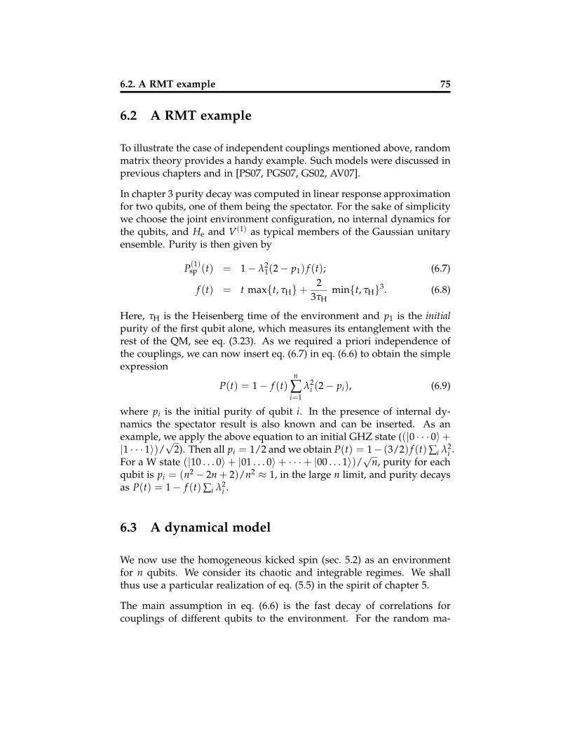
6.2. A RMT example 75
6.2 A RMT example
To illustrate the case of independent couplings mentioned above, randommatrix theory provides a handy example. Such models were discussed inprevious chapters and in [PS07, PGS07, GS02, AV07].
In chapter 3 purity decay was computed in linear response approximationfor two qubits, one of them being the spectator. For the sake of simplicitywe choose the joint environment configuration, no internal dynamics forthe qubits, and He and V(1) as typical members of the Gaussian unitaryensemble. Purity is then given by
P(1)sp (t) = 1− λ2
1(2− p1) f (t); (6.7)
f (t) = t max{t, τH}+2
3τHmin{t, τH}3. (6.8)
Here, τH is the Heisenberg time of the environment and p1 is the initialpurity of the first qubit alone, which measures its entanglement with therest of the QM, see eq. (3.23). As we required a priori independence ofthe couplings, we can now insert eq. (6.7) in eq. (6.6) to obtain the simpleexpression
P(t) = 1− f (t)n
∑i=1
λ2i (2− pi), (6.9)
where pi is the initial purity of qubit i. In the presence of internal dy-namics the spectator result is also known and can be inserted. As anexample, we apply the above equation to an initial GHZ state ((|0 · · · 0〉+|1 · · · 1〉)/
√2). Then all pi = 1/2 and we obtain P(t) = 1− (3/2) f (t) ∑i λ2
i .For a W state (|10 . . . 0〉+ |01 . . . 0〉+ · · ·+ |00 . . . 1〉)/
√n, purity for each
qubit is pi = (n2− 2n + 2)/n2 ≈ 1, in the large n limit, and purity decaysas P(t) = 1− f (t) ∑i λ2
i .
6.3 A dynamical model
We now use the homogeneous kicked spin (sec. 5.2) as an environmentfor n qubits. We consider its chaotic and integrable regimes. We shallthus use a particular realization of eq. (5.5) in the spirit of chapter 5.
The main assumption in eq. (6.6) is the fast decay of correlations forcouplings of different qubits to the environment. For the random ma-
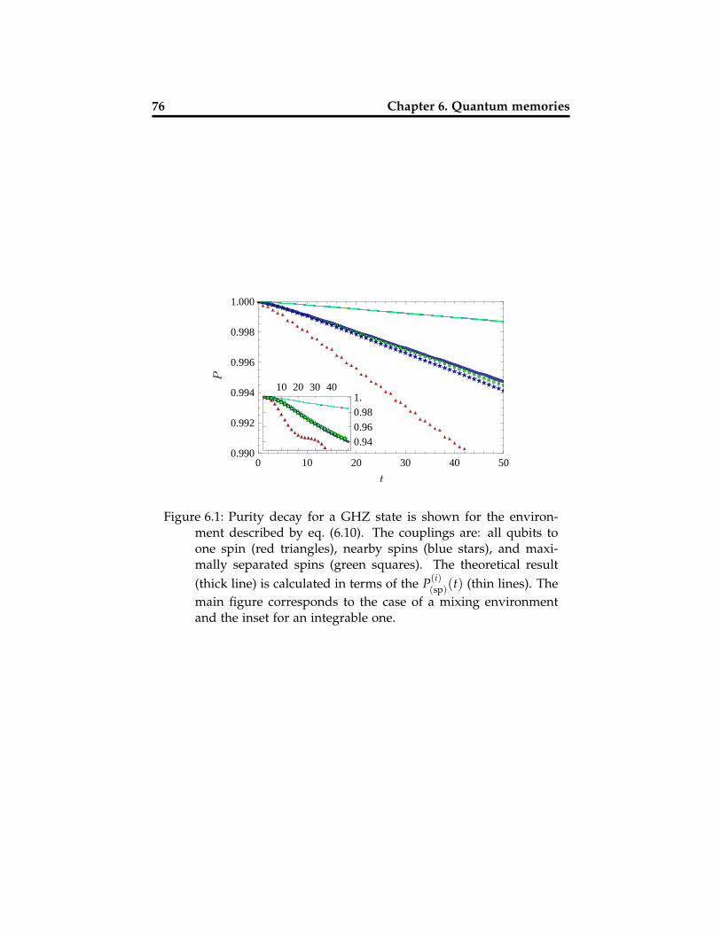
76 Chapter 6. Quantum memories
10 20 30 40
0.940.960.981.
0 10 20 30 40 500.990
0.992
0.994
0.996
0.998
1.000
t
P
Figure 6.1: Purity decay for a GHZ state is shown for the environ-ment described by eq. (6.10). The couplings are: all qubits toone spin (red triangles), nearby spins (blue stars), and maxi-mally separated spins (green squares). The theoretical result(thick line) is calculated in terms of the P(i)
(sp)(t) (thin lines). Themain figure corresponds to the case of a mixing environmentand the inset for an integrable one.
6.3. A dynamical model 77
trix model discussed above this is trivially fulfilled. Yet, integrable en-vironments are commonly used [CL83] and one may wonder whethereq. (6.6) can hold in such a context. We shall therefore study a dynamicalmodel where a few qubits are coupled to an environment representedby a kicked Ising spin chain using identical coupling operators for allqubits. In this model, the variation of the angle of the external kick-ing field allows the transition from a “quantum chaotic” to an integrableHamiltonian for the environment [Pro02, PP07](a). For convenience weseparate it in the environment and the central system. The Hamiltonianof the environment, namely the homogeneous kicked Ising spin chain,recall, is given by
H(e) =L−1
∑i=0
σ(e,i)x σ
(e,i+1)x + δ(t)
L−1
∑i=0
b · σ(e,i) (6.10)
where δ(t) = ∑n∈Z δ(t− n) (i.e. time is measured in units of the kick pe-riod), L the number of spins in the environment, σ(e,i) = (σ
(e,i)x , σ
(e,i)y , σ
(e,i)z )
the Pauli matrices of spin i, and b the dimensionless magnetic field withwhich the chain is kicked (h = 1). We close the ring requiring σ(e,L) ≡σ(e,0). The Hamiltonian of the QM is
H(qm) = δ(t) ∑i
b · σ(qm,i), (6.11)
where σ(qm,i) is defined similarly as for the environment. The coupling isgiven by
λV = λ ∑i
σ(qm,i)x σ
(e,ji)x . (6.12)
The ji’s define the positions where the qubits of the QM are coupled tothe spin chain. Equivalently we could use kicked Ising couplings and atime-independent field [PSW01].
To implement a chaotic environment, we use here b = (0.9, 0.9, 0). Weuse a ring consisting of L = 12 spins for the environment and 4 addi-tional spins for the qubits of the QM. The coupling strength is λ = 0.005.In Fig. 6.1, we study purity decay when all four qubits are coupled tothe same spin, to neighboring spins, and to maximally separated spins,~j = (0, 3, 6, 9). The initial state is the product of a GHZ state in the QMand a random pure state in the environment. We compare the resultswith eq. (6.6) (thick line) obtained from simulations of the spectator con-figuration (thin solid line). Coupling the spectator to different positions
78 Chapter 6. Quantum memories
in the chain yields near identical results for P(t), so we can see only oneline. The figure demonstrates the validity of eq. (6.6) for well separatedand hence independent couplings. For coupling to neighboring spins de-cay is slightly faster while the sum rule does not hold if all qubits arecoupled to the same spin.
A similar calculation for integrable environments with b = (0, 1.53, 0)yields faster purity decay than in the mixing case as expected from gen-eral considerations in [GPSZ06]. Nevertheless the sum rule is again wellfulfilled except if we couple all qubits to the same spin. This leads us tocheck the behavior of the correlation function
p[V(i)τ V(j)
τ′ $0 ⊗ $0] = 〈ψ0|V(i)τ V(j)
τ′ |ψ0〉. (6.13)
This is the simplest and usually largest term in A(i,j), eq. (6.5). Figure 6.2shows this quantity for chaotic (i.e. mixing) and integrable environmentsin the first and second row, respectively. The first column shows theautocorrelation function (i = j). The second and third columns give thecross correlation function (i 6= j) when the qubits are coupled to thesame or opposite spins, respectively. In the latter case, correlations arealways small thus showing that also in integrable situations our conditioncan be met. Non-vanishing correlations, as in fig. 6.2(b) and fig. 6.2(e)lead to deviations from the sum rule. The pronounced structure for theintegrable environment, fig. 6.2(e), may be associated to the oscillationsof purity decay (inset of fig. 6.1).
Another example where the conditions of our derivation are not met isthe following. A Bose-Einstein condensate in which the n atoms havetwo immiscible internal states [DDZ00] could be interpreted as a QM.The symmetry of the wave function reduces the dimension of the Hilbertspace and causes high correlations among the couplings to the environ-ment. It is not surprising then that decoherence scales differently (as n2).

6.3. A dynamical model 79
0. 0.2 0.4 0.6 0.8 1.
0 0 020 20 2040 40 400
0
20
20
40
40
τ
τ′
(a) (b) (c)
(d) (e) (f)
Figure 6.2: The color-coded absolute value of the real part of〈ψ0|V(i)
τ V(j)τ′ |ψ0〉 given in eq. (6.13) as a function of τ and τ′
for the chaotic [(a) (b) (c)] and the integrable [(d) (e) (f)] spinchain environment (L = 8). (a),(d) show the autocorrelationfunction (i = j); (b), (e) and (c) (f) the cross correlation func-tion for couplings to the same spin or opposite spins in the ringrespectively.

Chapter 7
Conclusions
We now proceed to formulate the conclusions of this work. We startby particular conclusions for each chapter, and afterwards to the generalconclusions and perspectives.
In chapter 2 we analyzed the decoherence (measured by purity duringall the thesis) of a single qubit immersed in an environment. For thispurpose we introduced a model with unitary dynamics in the qubit plusenvironment space. Both the environment Hamiltonian and the interac-tion were chosen as random matrices from the classical ensembles. Wesolved purity decay in terms of correlation functions of the environment.
We obtained linear and quadratic decay before and after the Heisenbergtime respectively. In general, purity of a superposition of eigenstatesdecays faster than an eigenstate. The presence of an internal Hamiltonianin the qubit was observed to contribute to stability. For the GOE case,different initial conditions in the Bloch sphere yield different behaviorsof purity and von Neumann entropy, even in the large environment limit.
Monte Carlo simulations showed that exponentiating the analytical for-mulae, as explained in appendix C, allowed extending the analytical re-sult outside the scope of linear response formalism.
In chapter 3 we used the spectator configuration (introduced in the in-troduction of the thesis), in which only a part (one qubit) of the centralsystem (two qubits) is coupled to an environment. This constituted thefirst of three models analyzed. We solve it using extensively the sym-metries of the ensembles. We found some elements in common with the
81

82 Chapter 7. Conclusions
single qubit case: the same qualitative dependence on time (linear andquadratic before and after the Heisenberg time, respectively; a depen-dence on an internal Hamiltonian, namely having a big energy splittingin the qubit increases stability; finally, a reasonable agreement with aheuristic exponentiation. With the second qubit we added a new ele-ment, entanglement. We observed that entanglement allowed taking theinvariance properties of one qubit into the other. We also observed thatentanglement induces a faster decoherence. For the TRI breaking case wefound that, due to entanglement, self averaging is expected when usingBell states.
The other two models (joint environment and separate environment),which possess a very different physical interpretation, were reduced tothe spectator configuration using the independence of the couplings. Theirbehavior is similar, up to a scaling of the coupling constant.
In chapter 4 we studied, for two qubits coupled to an environment, therelation between purity and concurrence as both evolve in time. Both theenvironment and the coupling are chosen from the classical ensembles.In order to analyze their relation we introduce the CP plane. We foundthat in the large dimension limit of the environment, concurrence andpurity are restricted to a small region defined using unital channels. Infact, in the large dimension limit, for all parameters studied, the chan-nels induced by the random Hamiltonian approach rapidly the unitalitycondition. For large purities the allowed unital region is almost one di-mensional, which allows to write a one to one relation for concurrenceand purity. In some cases the curve described by the system in the CPplane coincides with the Werner curve. The deviation from it, for a partic-ular level splitting in the coupled qubit, is given in an empirical formulawhich depends on the coupling strength and the size of the environment.This deviation goes rapidly to zero as the size of the environment and thecoupling increase. Assuming that purity and concurrence are related viathe Werner curve, it is possible to use our knowledge from the previouschapters to give a formula for concurrence decay.
In chapter 5 we studied the same problem as in previous chapters (oneand two qubit decoherence), but using particular dynamical models. Themodels consists of n spins interacting pairwise with individually ad-justable strengths, and kicked with a magnetic field. The dynamical sys-tem is flexible enough to allow different configurations and symmetriesof the environment and coupling. Moreover, varying the parameters we

83
can have qualitatively different kinds of dynamics, namely chaotic, in-termediate and integrable. In the chaotic regime of the environment weobtained quantitative agreement with the RMT formulae obtained earlierfor purity decay. For the integrable case we observed quadratic decay,sometimes with strong revivals (when the coupling was to an open endof a chain). The intermediate case displays oscillations superimposed toa linear decay. In the chaotic case we observe that the effective Heisen-berg time (determined, among other things, by the symmetry of both theenvironment and the coupling) plays an important roll in decoherence.
Purity and concurrence behave in a qualitatively similar way for all con-figurations. The relation between the two, for sufficiently large envi-ronments, follows an analytic expression we get for Werner states quiteclosely, although the specific dynamics does not produce Werner states.
Finally, in chapter 6 we calculated generic decoherence of a n-qubit quan-tum memory as represented by purity decay. For large purities it is glob-ally given in linear response approximation by a sum rule in terms of thepurities of the individual qubits entangled with the remaining register asspectator. This sum rule depends crucially on the absence or rapid decayof correlations between the couplings of different qubits in the interactionpicture. We prove that this is fulfilled by sufficiently chaotic environmentsor couplings but, using a spin chain model as an environment, we findthat even if the latter is integrable correlations can be absent and the sumrule holds. While exceptions can be constructed we have a very generaltool to reduce the decoherence of a QM of n qubits to the problem of asingle qubit entangled with the rest of the QM. Furthermore the result isequally valid if we perform local operations on the qubits.
Some possible extensions or generalizations of the thesis are now out-lined.
• Several measures for entanglement of multi-qubit systems exist. De-pending on the particular problem to be treated, one or the othermight be useful. Preliminary results [ste] indicate that for multi-qubit systems a relation, like the one found for two qubits, mightbe used to obtain formulae for entanglement decay.
• In order to deepen our knowledge of the behavior of integrable andintermediate systems, one should study particular models.
• As many interactions are indeed separable, a RMT formulation for

84 Chapter 7. Conclusions
separable interactions of the qubit(s) with the environment mightproof useful to understand the similarities and differences with this“more realistic” coupling.
• The sum rule studied in chapter 6 also applies if the register is splitinto arbitrary sets of qubits. In fact, one and two qubit gates areknown to be universal for quantum computation [NC00], so we laythe foundation for the computation of decoherence during the ex-ecution of a general algorithm. This extension only requires theknowledge of the decoherence of a pair suffering the gate operationwhile entangled with the rest of the register. As each gate is dif-ferent, we will have to take a step by step approach, which at eachstep will only involve one and two qubit decoherence. The linearresponse approximation will be sufficient due to the high fidelityrequirements of quantum computation.
Summarizing, we have developed a tool to study decoherence of qubitsbased on the spectator configuration and on random matrix theory. Wehave compared the results found with a kicked Ising model. We almost al-ways observed linear/quadratic decay of purity before/after the Heisen-berg time of the environment and self averaging both with respect to theHamiltonian and to the initial conditions. The exceptions are: (i) In thepresence of an internal Hamiltonian, the central system eigenstates decaylinearly even after Heisenberg time. (ii) If we have a time reversal invari-ant Hamiltonian, no self averaging with respect to the initial conditionsis observed after the Heisenberg time. (iii) In the KI model, and presum-ably due to the separable structure of the Hamiltonian, no self averaging,before the Heisenberg time, was observed. Entanglement enhances de-coherence and may transport symmetry properties from one qubit to theother. When studying two qubits we also studied their internal entangle-ment, as quantified by concurrence. A one to one correspondence wasoften found, characterized by the Werner curve. Thus, formulae for en-tanglement decay are also available. For a larger number of qubits a sumrule can be applied in a wide range of circumstances to express puritydecay of a group of particles in terms of purity decay of each particle ina spectator configuration. In all cases, heuristic exponentiation leads togood agreement beyond linear response scope.

Appendix A
One-qubit purity decay forpure and mixed states
Here, we consider the one-qubit decoherence in a more general context.One-qubit decoherence as described in sec. 2 deals with a separable initialstate $0 = ρ1 ⊗ |ψe〉〈ψe|, ρ1 = |ψ1〉〈ψ1|. Thus $0 is a pure state of a singlequbit coupled to an environment in the pure state |ψe〉. We consider herearbitrary, finite dimensions of H1 and He, and we allow ρ1 to be mixed.The latter poses some problems on the physical interpretation of purityas a measure for decoherence. However, these can be avoided by takingthe point of view of the environment, as it becomes entangled with thecentral system. That means we consider the purity of the state of the en-vironment after tracing out the central-system’s degrees of freedom; seeeq. (3.10) and eq. (3.11). If we consider the entanglement with a specta-tor being responsible for the mixedness of ρ1, we can use the followingresults to describe purity decay in the spectator model.
We will derive explicit expressions for the average purity 〈P(t)〉 as a func-tion of time, where the average is only over the random coupling. Theseexpressions involve a few elemental spectral correlation functions, whoseproperties will be discussed in A.5. As detailed in sec. 2.2, we work withthe echo operator M(t) in the linear response approximation eq. (2.9).Note that I(t) is Hermitian, while, due to time-order inversion, J(t) isnot.
This section is slightly boring, but since this is a Ph.D. thesis, the detailsmust be incorporated. My thanks an admiration to the devoted reader
85

86 Appendix A. One-qubit purity decay for pure and mixed states
who reached this section.
A.1 General calculation
Let $1 and $2 be two operators acting on the Hilbert space H′ = H1⊗He.We define the purity form p[ · ] as a function of pairs of such operators,
p[$1 ⊗ $2] = tre[tr1($1) tr1($2)] . (A.1)
Since any linear operator acting on H′ ⊗H′ can be expanded in termsof separable operators of the form $1 ⊗ $2, linearity implicitly defines thepurity form for arbitrary linear operators. For arbitrary operators A, Bacting both on H′, the purity form has the following property:
p[A⊗ B] = p[A† ⊗ B†]∗ = p[B⊗ A] = p[B† ⊗ A†]∗ . (A.2)
The purity defined in eq. (1.8) can be expressed in terms of the purityform as
P(tre $) = p[$⊗ $] . (A.3)
Note that on the RHS of this equation, we first take the trace over thecentral system, i.e. we consider the purity of the state of the environmentafter tracing out the central degrees of freedom. With this little twist wecan describe the one-qubit decoherence and the spectator model at thesame time.
To average purity, we use eq. (2.9) to compute $M(t) ⊗ $M(t) in linearresponse approximation
〈P(t)〉 = 〈 p[$M(t)⊗ $M(t)] 〉 = p[〈$M(t)⊗ $M(t)〉] . (A.4)
Keeping terms only up to second order in λ:
$M(t)⊗ $M(t) = $0 ⊗ $0 (A.5)
− iλ[
I$0 ⊗ $0 − $0 I† ⊗ $0 + $0 ⊗ I$0 − $0 ⊗ $0 I]†
− λ2[
J$0 ⊗ $0 + $0 J† ⊗ $0 + $0 ⊗ J$0 + $0 ⊗ $0 J]†
+ λ2[I$0 I† ⊗ $0 − I$0 ⊗ I $0 + I$0 ⊗ $0 I†
+ $0 I† ⊗ I$0 − $0 I† ⊗ $0 I† + $0 ⊗ I $0 I†].
A.1. General calculation 87
In the next step, we perform the ensemble average over the coupling. Theodd terms in λ vanish as purity (even without averaging) must be real.For the remaining terms, we use the properties in eq. (A.2) and the factthat I(t) is Hermitian, to obtain
〈P(t)〉 = P(0)− λ2(AJ − AI) (A.6)
with P(0) = p[$0 ⊗ $0] and
AJ = 4 Rep[〈J〉$0 ⊗ $0]AI = 2 (p[〈I$0 I〉 ⊗ $0]− Rep[〈I$0 ⊗ I$0〉] + p[〈I$0 ⊗ $0 I〉]) . (A.7)
In order to pull out the same double integral of AJ and AI , we use thetime ordering symbol T . It allows to write for the average purity as afunction of time
〈P(t)〉 = P(0)− 2λ2∫ t
0dτ∫ t
0dτ′ Re AJI (A.8)
with
AJI = p[T 〈VV ′〉$0 ⊗ $0]− p[〈V ′$0V〉 ⊗ $0]+ p[〈V$0 ⊗ V ′$0〉]− p[〈V ′$0 ⊗ $0V〉] , (A.9)
where V and V ′ are short forms for the coupling matrices V(τ) and V(τ′),respectively. The arguments τ and τ′ of the coupling matrices are inter-changed in the second and fourth term of AJI. This does not change thevalue of the integral of course, but it facilitates to handle common termsin the following considerations.
The integrand AJI in eq. (A.9) consists of four terms. These terms will beconsidered, one after the other. We will always first average the argumentof the purity form. Only then we perform the partial traces over subsys-temH1, and therefore the final trace over the environment. The averagingis only over the coupling, and it is done by applying two simple rules, asdescribed below.
For the coupling V1,e in the product eigenbasis of H0, we use either ran-dom Gaussian unitary (GUE) or orthogonal (GOE) matrices. Their sta-tistical properties are completely characterized by the following secondmoments (for notational ease we ignore the subscript 1,e for a moment)
〈VijVkl〉 = δil δjk + χGOE δik δjl , (A.10)

88 Appendix A. One-qubit purity decay for pure and mixed states
where χGOE = 1 if V is taken from the GOE, while χGOE = 0 if V is takenfrom the GUE. In the interaction picture we then find:
〈Vij Vkl〉 =(
δil δjk e−i(Ej−Ei) (τ−τ′) + χGOE δik δjl e−i(Ej−Ei) (τ+τ′) ) . (A.11)
A.2 The GUE case
We now procede to calculate one by one the contributions.
p[T 〈V V ′〉$0⊗ $0](t): We first compute the average
T 〈VV ′$0 ⊗ $0〉 = ∑ijklmn
|ij〉 T 〈V(τ)ij,klV(τ′)kl,mn〉〈mn|$0 ⊗ $0
= ∑ijkl|ij〉e−i(Ekl−Eij)|τ−τ′|〈ij|$0 ⊗ $0, (A.12)
where we have used the averaging rule, eq. (A.11), as well as the fact thatthe time-ordering operator T requests to exchange τ with τ′ wheneverτ < τ′. The indices i, k and m denote basis states in H1, while the indicesj, l and n denote basis states in He. We can rewrite that expression in amore compact form by employing the diagonal matrices Cx(τ), definedin eq. (A.37):
T 〈VV ′$0 ⊗ $0〉 =(C1(|τ − τ′|)⊗ Ce(|τ − τ′|)
)× (ρ1 ⊗ |ψe〉〈ψe|)⊗ (ρ1 ⊗ |ψe〉〈ψe|) . (A.13)
Now we apply the partial traces over subsystem H1
tr1(〈V V ′〉 $0
)tr1 $0 = C1(|τ − τ′|) Ce(|τ − τ′|) |ψe〉 〈ψe| . (A.14)
The final trace over the environment yields
p[T 〈V V ′〉$0 ⊗ $0](t) = C1(|τ − τ′|) Ce(|τ − τ′|) . (A.15)
p[〈V ′$0V〉 ⊗ $0](t): We first compute the average
〈V ′$0V〉 ⊗ $0 = ∑ijklmnpq
|ij〉⟨
V ′ij,kl〈kl|$0|mn〉Vmn,pq
⟩〈pq| ⊗ $0
= ∑ijkl|ij〉e−i(Eij−Ekl)(τ−τ′)〈kl|$0|kl〉〈ij| ⊗ $0, (A.16)
A.2. The GUE case 89
where we have used eq. (A.11). We apply the partial traces over subsys-tem H1
tr1(〈V ′$0V〉
)tr1 $0 =
(∑ik
e−i(Ei−Ek)(τ−τ′)〈k|ρ1|k〉)
(A.17)
×∑jl|j〉e−i(Ej−El)(τ−τ′)〈l|ψe〉〈ψe|l〉〈j|ψe〉〈ψe|
= C1(τ − τ′) ∑jl|j〉 e−i(Ej−El) (τ−τ′)
× 〈l|ψe〉 〈ψe|l〉 〈j|ψe〉 〈ψe|.The final trace over the environment yields
p[〈V ′$0V〉 ⊗ $0] = C1(τ − τ′) ∑jl〈ψe|l〉eiEl(τ−τ′)〈l|ψe〉〈ψe|j〉e−iEj(τ−τ′)〈j|ψe〉
= C1(τ − τ′)Se(τ − τ′), (A.18)
where Sx(τ) is defined in eq. (A.39).
p[〈V$0⊗ V ′$0〉](t): We first compute the average
〈V $0 ⊗ V ′ $0〉 = ∑ij kl mn pq
|ij〉⟨Vij,kl 〈kl| $0 ⊗ |mn〉 Vmn,pq
⟩〈pq| $0
= ∑ij kl|ij〉 e−i(Ekl−Eij) (τ−τ′) 〈kl| $0 ⊗ |kl〉 〈ij| $0 . (A.19)
Then we apply the partial traces over subsystem H1⟨tr1(
V $0)
tr1(
V ′ $0) ⟩
=(
∑ike−i(Ek−Ei) (τ−τ′) 〈k|ρ1|i〉 〈i|ρ1|k〉)
×∑jl|j〉 e−i(El−Ej) (τ−τ′) 〈l|ψe〉 〈ψe|l〉 〈j|ψe〉 〈ψe| .
The final trace over the environment yields
p[〈V$0 ⊗ V ′$0〉] = S1(τ − τ′) Se(τ − τ′) . (A.20)
p[〈V ′$0⊗ $0V〉](t): We first compute the average
〈V ′ $0 ⊗ $0 V〉 = ∑ij kl mn pq
|ij〉⟨
V ′ij,kl 〈kl| $0 ⊗ $0 |mn〉 Vmn,pq
⟩〈pq|
= ∑ij kl|ij〉 e−i(Eij−Ekl) (τ−τ′) 〈kl| $0 ⊗ $0 |kl〉 〈ij| (A.21)
90 Appendix A. One-qubit purity decay for pure and mixed states
We apply the partial traces over subsystem H1⟨tr1(
V $0)
tr1(
$0 V ′) ⟩
=(
∑ike−i(Ei−Ek) (τ−τ′) 〈k|ρ1|i〉 〈i|ρ1|k〉)
×∑jl|j〉 e−i(Ej−El) (τ−τ′) 〈l|ψe〉 〈ψe|l〉 〈j| .
The final trace over the environment yields
p[〈V$0 ⊗ $0V ′〉] = S1(τ − τ′) Ce(τ − τ′) . (A.22)
A.3 The GOE case
In the GOE case, the average over the coupling yields, besides the pre-viously considered GUE-term an additional one; see eq. (A.11). In thefollowing we will redo the calculation of the previous subsection, butconsider only that additional term. As a reminder, we add the subscript2 to the brackets which denote the ensemble average.
p[T 〈V V ′〉2$0⊗ $0](t): We first compute the average
T 〈V V ′〉2 $0 ⊗ $0 = ∑ij kl mn
|ij〉 T 〈V(τ)ij,kl V(τ′)kl,mn〉2 〈mn| $0 ⊗ $0
= ∑ij|ij〉 〈ij| $0 ⊗ $0 (A.23)
= $0 ⊗ $0 , (A.24)
where we have used the averaging rule, eq. (A.11). Here the time-orderingoperator has no effect. Now we apply the partial traces over subsystemH1
tr1(〈V V ′〉2 $0
)tr1 $0 = |ψe〉 〈ψe| . (A.25)
The final trace over the environment yields
p[〈V V ′〉2$0 ⊗ $0](t) = 1 . (A.26)
p[〈V ′$0V〉2⊗ $0](t): We first compute the average
〈V ′ $0 V〉2 ⊗ $0 = ∑ij kl mn pq
|ij〉⟨
V ′ij,kl 〈kl|$0|mn〉 Vmn,pq
⟩2〈pq| ⊗ $0
= ∑ij kl|ij〉 e−i(Eij−Ekl) (τ+τ′) 〈kl|$0|ij〉 〈kl| ⊗ $0 , (A.27)

A.3. The GOE case 91
where we have used eq. (A.11). We apply the partial traces over subsys-tem H1
tr1(〈V ′ $0 V〉2
)tr1 $0 = ∑
jl|j〉 e−i(Ej−El) (τ+τ′) 〈l|ψe〉 〈ψe|j〉 〈l|ψe〉 〈ψe| .
(A.28)The final trace over the environment yields
p[〈V ′$0V〉 ⊗ $0] = ∑jl〈l|ψe〉 eiEl (τ+τ′) 〈l|ψe〉 〈ψe|j〉 e−iEj (τ+τ′) 〈ψe|j〉
= S′e(−τ − τ′) , (A.29)
where S′x(τ) is defined in eq. (A.40).
p[〈V$0⊗ V ′$0〉2](t): We first compute the average
〈V $0 ⊗ V ′ $0〉2 = ∑ij kl mn pq
|ij〉⟨Vij,kl 〈kl| $0 ⊗ |mn〉 Vmn,pq
⟩2 〈pq| $0
= ∑ij kl|ij〉 e−i(Ekl−Eij) (τ+τ′) 〈kl| $0 ⊗ |ij〉 〈kl| $0 . (A.30)
Then we apply the partial traces over subsystem H1⟨tr1(V$0
)tr1(V ′$0
)⟩2 =
(∑ike−i(Ek−Ei)(τ+τ′)〈k|ρ1|i〉〈k|ρ1|i〉
)×∑
jl|j〉e−i(El−Ej)(τ+τ′)〈l|ψe〉〈ψe|j〉〈l|ψe〉〈ψe|. (A.31)
The final trace over the environment yields
p[〈V$0 ⊗ V ′$0〉2] = S′1(τ + τ′) S′e(τ + τ′) . (A.32)
p[〈V ′$0⊗ $0V〉2](t): We first compute the average
〈V ′ $0 ⊗ $0 V〉2 = ∑ij kl mn pq
|ij〉⟨
V ′ij,kl 〈kl| $0 ⊗ $0 |mn〉 Vmn,pq
⟩2〈pq|
= ∑ij kl|ij〉 e−i(Eij−Ekl) (τ+τ′) 〈kl| $0 ⊗ $0 |ij〉 〈kl| . (A.33)
We apply the partial traces over subsystem H1⟨tr1(
V $0)
tr1(
$0 V ′) ⟩
2 =(
∑ike−i(Ei−Ek) (τ+τ′) 〈k|ρ1|i〉 〈k|ρ1|i〉)
×∑jl|j〉 e−i(Ej−El) (τ+τ′) 〈l|ψe〉 〈ψe|j〉 〈l| .
92 Appendix A. One-qubit purity decay for pure and mixed states
The final trace over the environment yields
p[〈V$0 ⊗ $0V ′〉2] = S′1(−τ − τ′) . (A.34)
A.4 The general solution
If the coupling matrix is taken either from the Gaussian unitary (GUE) ororthogonal (GOE) ensemble, we find
AJI =[
C1(|τ − τ′|)− S1(τ − τ′)] [
Ce(|τ − τ′|)− Se(τ − τ′)]
+ χGOE[1− S′e(−τ − τ′) + S′1(τ + τ′)S′e(τ + τ′)− S′1(−τ − τ′)
]. (A.35)
These expressions are derived from the previous two sections, for theGUE case in A.2, for the GOE case in A.3. The correlation functionsCx, Sx, C′x and S′x with x ∈ {1, e} are defined and discussed in A.5.
If the dimension of the Hilbert space of the environment goes to infinity,the corresponding correlation functions simplify, as discussed in A.5. Weare then left with
AJI =[
C1(|τ − τ′|)− S1(τ − τ′)]
C(|τ − τ′|) + χGOE[
1− S′1(−τ − τ′)]
.(A.36)
A.5 Some particular correlation functions
Averaging over the perturbation (i.e. the coupling) leads to expressionswhich may involve the diagonal matrix
Cx(τ) = ∑ik|i〉 e−i(Ek−Ei) τ 〈i| x ∈ 1, e . (A.37)
Here, x denotes one of the two subsystems, either the qubit or the en-vironment. Evidently, the energies Ek are the eigenvalues of the corre-sponding Hamiltonian. In the derivations in this appendix, the expecta-tion value of Cx(τ) with respect to the initial state $0 = ρ1 ⊗ ρe are ofparticular importance. These are denoted by
Cx(τ) = tr(
Cx(τ) ρx)
x ∈ 1, e . (A.38)
A.5. Some particular correlation functions 93
In this work, ρe = |ψe〉〈ψe| is always a pure state.
We will also encounter another type of correlation function, which maybe defined as follows
Sx(τ) = trx[
e−iHx τ ρx eiHx τ ρx]
. (A.39)
If the initial state ρx is pure, this quantity becomes the return probability.At τ = 0 it gives the purity of ρx. In the case of GOE averages, we alsoencounter the correlation function
S′x(τ) = trx[
e−iHx τ ρx eiHx τ ρTx ,]
. (A.40)
In the main part of this paper, we focus on the limit, where the dimensionof the environment(s) becomes infinite. In that case it makes sense toperform an additional spectral average over He and/or He′ . In the case ofCe(t) this yields
〈Ce(τ)〉 = C(τ) 11eC(τ) = 〈Ce(τ)〉 = 1 + δ(τ/τH)− b(β)2 (τ/τH) , (A.41)
where b(β)2 (t) is the two-point spectral form factor with time measured
in units of the Heisenberg time τH for the corresponding spectral ensem-ble. In the limit of large dimension Ne = dim(He) we find for the othercorrelation functions:
Se(τ) = tr(
e−iHeτ|ψe〉〈ψe|eiHeτ|ψe〉〈ψe|)
(A.42)
S′e(τ) = tr(
e−iHeτ|ψe〉〈ψe|eiHeτ|ψ∗e 〉〈ψ∗e |)
. (A.43)
For random pure states, as considered in the present work, both correla-tion functions are at most of order one at τ = 0. For τ > 0 they dropvery quickly and soon become of order N−1
e . This happens on the sametime scale, where Ce(τ) drops from values of the order Ne to values ofthe order one. In that sense we consider these correlation functions tocontribute only O(N−1
e ) corrections to the result given in eq. (A.36).
A single qubit is a two level system. The most general pure initial stateis given by |a〉 = |1〉 a1 + |2〉 a2, with |a1|2 + |a2|2 = 1. The most gen-eral mixed state is given by ρ1 = λ1 |a〉 〈a| + λ2 |b〉 〈b|, with λ1, λ2 ≥ 0,real, λ1 + λ2 = 1, and |a〉, |b〉 arbitrary pure states with 〈a|b〉 = 0. Wewill now investigate the behaviour of the different correlation functionsReC1(τ), S1(τ), and S′1(τ) as it depends on the initial state and the Hamil-tonian H1 = |1〉E1〈1|+ |2〉E2〈2|.
94 Appendix A. One-qubit purity decay for pure and mixed states
(a) Assume ρ1 = |a〉 〈a|. Then
C1(τ) = ∑ik|ai|2 e−i(Ek−Ei) τ = 1 + cos ∆τ + i(|a2|2 − |a1|2) sin ∆τ ,
(A.44)holds, so
Re C1(τ) = 1 + cos ∆τ ∆ = E2 − E1 . (A.45)
(b) For ρ1 = λ1 |a〉 〈a|+ λ2 |b〉 〈b| we still have
Re C1(τ) = 1 + cos ∆τ . (A.46)
(c) Assume ρ1 = |a〉 〈a|. Then we find for S1(τ) = s(|a〉; τ)
S1(τ) = ∑ik|ai|2|ak|2 e−i(Ei−Ek) τ = |a1|4 + |a2|4 + 2 |a1|2|a2|2 cos ∆τ .
(A.47)This expression only depends on the absolute values squared of thecoefficients a1 and a2. Therefore we may parametrize them withoutloss of generality as a1 = cos φ and a2 = sin φ. We then find
S1(τ) = gφ + (1− gφ) cos ∆τ gφ = |a1|4 + |a2|4 = 1− 12
sin2 2φ .(A.48)
(d) For a general mixed state ρ1 = λ1 |a〉 〈a|+ λ2 |b〉 〈b| we find
S1(τ) = λ21 s(|a〉; τ) + λ2
2 s(|b〉; τ) + 2 λ1λ2 ∑ik
aia∗k bkb∗i cos(Ei − Ek)τ
= λ21 s(|a〉; τ) + λ2
2 s(|b〉; τ)+
4 λ1λ2 |a1|2|b1|2(
1− cos ∆τ), (A.49)
where we have used that 〈a|b〉 = a1b∗1 + a2b∗2 = 0. Note that the co-efficients a1, a2, b1, b2 may be arranged into a square unitary matrix,and must therefore be of the following general form(
a1 b1a2 b2
)= eiϑ
(eiξ cos φ eiχ sin φ− e−iχ sin φ e−iξ cos φ
). (A.50)
This shows that s(|a〉; τ) = s(|b〉; τ) = gφ + (1− gφ) cos ∆τ, and that
S1(τ) = (λ21 + λ2
2)[
gφ + (1− gφ) cos ∆τ]
+ 2 λ1λ2 (1− gφ)(
1− cos ∆τ)
. (A.51)

A.5. Some particular correlation functions 95
Since λ1 + λ2 = 1 it is convenient to set λ1 = cos2 θ and λ2 = sin2 θsuch that we may write λ2
1 + λ22 = gθ and obtain
S1(τ) = 1− gθ − gφ + 2 gθ gφ + (2gθ − 1)(1− gφ) cos ∆τ . (A.52)
(e) Assume again that ρ1 = |a〉 〈a|. Then we find for S′1(τ) = s′(|a〉; τ)
S′1(τ) = |a1|4 + |a2|4 + a21(a∗2)
2 ei∆τ + a22(a∗1)
2 e−i∆τ
= gφ + 2 |a1|2|a2|2 cos(∆τ + 2η)= gφ + (1− gφ) cos(∆τ + 2η) η = arg(a1)− arg(a2) . (A.53)
However, as discussed in sec. 2.5, a natural symmetry around the yaxis (in the Bloch sphere picture) appears for ∆ = 0. In that case,using γ as defined in that section, one can prove that
1− S′1(τ)∣∣∆=0 = (1− gφ)[1− cos(2η)] = sin2 γ (A.54)
using elementary geometric and trigonometric considerations.
(f) For a general mixed state ρ1 = λ1 |a〉 〈a|+ λ2 |b〉 〈b| we find
S′1(τ) = λ21 s′(|a〉; τ)+ λ2
2 s′(|b〉; τ)+ 2 λ1λ2 Re ∑ik
aia∗k b∗k bi e−i(Ei−Ek) τ .
(A.55)It follows from eq. (A.50) that arg(b1)− arg(b2) = arg(a1)− arg(a2)−π, such that the equality s′(|a〉; τ) = s′(|b〉; τ) holds, just as in thecase of S1(τ). Therefore we may write
S′1(τ) = gθ
[gφ + (1− gφ) cos(∆τ + 2η)
](A.56)
+ 2 λ1λ2 (1− gφ) Re(
1 + ei(∆τ+2η−π) )= 1− gθ − gφ + 2 gθ gφ + (2gθ − 1)(1− gφ) cos(∆τ + 2η) .
(A.57)
Note that the only difference to S(τ) in case (d) is the additionalphase 2η in the argument of the cosine function. Using the sameangle γ defined with eq. (3.26), in complete analogy with eq. (2.23),and using eq. (A.54) we obtain
1− S′1(τ)∣∣∆=0 = 1− gθ + (2gθ − 1) sin2 γ. (A.58)


Appendix B
Implementing the evolution ofthe KI models
In this appendix we describe how to implement numerically Hamilto-nians describing a set of qubits with pairwise variable Ising interaction,and kicked with a periodic, and site dependent, magnetic field. We haveused this systems in chapters 5 and 6, the reason being (i) the flexibilityof the dynamical model to describe various physical situations, (ii) it hasvarious dynamical regimes, and (iii) it is has an efficient implementationmaking it useful for numerical studies.
Recall eq. (5.5), the Hamiltonian of the system is
H =L
∑j>k=1
Jj,kσzj σz
k + δ1(t)L
∑j=1
~bj ·~σj. (B.1)
which gives rise to the Floquet operator UKI = UIsingUkick with
UIsing = exp
(−i
L
∑j>k=1
Jj,kσzj σz
k
), Ukick = exp
(−i
L
∑j=1
~bj ·~σj
). (B.2)
However notice that
UIsing =L
∏j>k=1
exp(−iJj,kσz
j σzk
), Ukick =
L
∏j=1
exp(−i~bj ·~σj
)(B.3)
Thus the evolution operator is decomposed trivially into single and twoqubit operators that can be efficiently implemented in a computer. Notice
97

98 Appendix B. Implementing the evolution of the KI models
that we do not need to explicitly diagonalize or even store the completeevolution operator thus allowing the implementation of twice as muchspins than with brute force diagonalization.
The state can be stored in a complex array with indices ranging from 0 to2L − 1. The state (expressed in the computational basis)
|ψ〉 =1
∑iL−1,iL−2,··· ,i0=0
αiL−1iL−2···i0 |iL−1iL−2 · · · i0〉, (B.4)
can be stored in a complex array of dimension 2L, if in the position ∑j ij2j
we store the value αiL−1iL−2···i0 . A Fortran 90 routine implementing theIsing interaction with the state stored in this form is the following.
subroutine Action_Ising_Interaction(psi,l,m,J)complex(kind(1d0)),intent(inout) :: psi(0:)real(kind(1d0)),intent(in) :: Jinteger,intent(in) :: l,minteger :: ido i=0,size(psi)-1If(btest(i,l).eqv.btest(i,m)) thenpsi(i)=exp(-(0d0,1d0)*J)*psi(i)elsepsi(i)=exp((0d0,1d0)*J)*psi(i)end Ifend doend subroutine Action_Ising_Interaction
A routine to implement the magnetic kick is now presented.
subroutine Application_Of_Kick(psi,b,l)complex(kind(1d0)),intent(inout) :: psi(0:)real(kind(1d0)),intent(in) :: b(:)complex(kind(1d0)) :: Matrix_For_Kick(2,2)complex(kind(1d0)) :: z(2)integer,intent(in) :: linteger :: j_left,j_right,left_digitinteger :: UpperNumber,LowerNumberif(sum(b**2).eq.0d0) returnMatrix_For_Kick=Matrix_For_Magnetic_Kick(b)

99
do j_left=0,size(psi)/2**(1+l)-1left_digit=ishft(j_left,l+1)do j_right=0,2**l-1LowerNumber=left_digit+j_rightUpperNumber=IBset(LowerNumber,l)z(1)=psi(LowerNumber); z(2)=psi(UpperNumber)z=MatMul(Matrix_For_Kick,z)psi(LowerNumber)=z(1); psi(UpperNumber)=z(2)end doend doend subroutine Application_Of_Kick
The previous routine uses the following function.
function Matrix_For_Magnetic_Kick(b)complex(kind(1d0)) :: Matrix_For_Magnetic_Kick(2,2)real(kind(1d0)),intent(in) :: b(3)real(kind(1d0)) :: n(3),phi,cosphis2,sinphis2phi=norma(b); n=b/phiMatrix_For_Magnetic_Kick(1,1)=&
cos(phi)-(0d0,1d0)*n(1)*sin(phi)Matrix_For_Magnetic_Kick(2,2)=&
conjg(Matrix_For_Magnetic_Kick(1,1))Matrix_For_Magnetic_Kick(1,2)=&
-(n(3)+(0d0,1d0)*n(2))*sin(phi)Matrix_For_Magnetic_Kick(2,1)=&
-conjg(Matrix_For_Magnetic_Kick(1,2))end function Matrix_For_Magnetic_Kick


Appendix C
The exponentiation
The linear response formulae for purity derived throughout the thesisare expected to work for high purities or, equivalently, when the firsttwo terms in the series eq. (2.9) approximate the echo operator well; itis of obvious interest to extend them to cover a larger range. The exactsolution for fidelity decay has, in some cases, been possible with someeffort, using super-symmetry techniques. This has been partly due to thesimple structure of fidelity, but trying to use this approach for a morecomplicated object such as purity seems to be out of reach for the timebeing. Exponentiating the formulae obtained from the linear responseformalism has proved to be in good agreement with the exact super-symmetric and numerical results for fidelity, if the perturbation is not toobig. The exponentiation of the linear response formulae for purity can becompared with Monte Carlo simulations in order to prove its validity. Wewish to explain the details required to implement this procedure in thisappendix.
Given a linear response formula PLR(t) [for which P(0) = 1], and anexpected asymptotic value for infinite time P∞, the exponentiation reads
PELR(t) = P∞ + (1− P∞) exp[−1− PLR(t)
1− P∞
]. (C.1)
This particular form guaranties that
PELR(t) ≈ PLR(t) (C.2)
for short times, and that
limt→∞
PELR(t) = P∞. (C.3)
101

102 Appendix C. The exponentiation
The particular value of P∞ will depend on the physical situation; in ourcase it will depend on the configuration and on the initial condition. Wenow turn to an estimation of this quantity for the spectator configuration,under some very general assumptions.
Let us write the initial condition in the qubits as
|ψ12(θ)〉 = cos θ|0102〉+ sin θ|1112〉 (C.4)
for some rotated qubits |0i〉, |1i〉. We assume that for long enough times,decoherence is described for the uncoupled qubit by the following chan-nel:
Etd[ρ] =112
=14(σxρσx + σyρσy + σzρσz + ρ
). (C.5)
This is the depolarizing channel with full strength [NC00]. This channelis unital. We now evaluate Etd ⊗ 11[|ψ12(θ)〉〈ψ12(θ)|]. Note that Etd ⊗11[|00〉〈00|] = 11⊗ |0〉〈0|/2 and Etd ⊗ 11[|11〉〈11|] = 11⊗ |1〉〈1|/2. For thecross terms we obtain:
Etd ⊗ 11[|00〉〈11||] =|10〉〈01| − |10〉〈01| − |00〉〈11|+ |00〉〈11|
4= 0, (C.6)
and also Etd⊗ 11[|11〉〈00||] = 0. Using the linearity of the channel and theresults found, we see that
Etd ⊗ 11[|ψ12(θ)〉〈ψ12(θ)|] =12
cos2 θ 0 0 0
0 cos2 θ 0 00 0 sin2 θ 00 0 0 sin2 θ
. (C.7)
In the end, we estimate the asymptotic value of purity as
P∞ =cos4 θ + sin4 θ
2=
gθ
2, (C.8)
where gθ was defined in eq. (2.17).
For both the joint and the separate environment configuration we use thevalue
P∞ = P (Ed ⊗ Ed[|ψ12(θ)〉〈ψ12(θ)|]) =14
. (C.9)
Good agreement is found with Monte Carlo simulations for moderate andstrong couplings. Obtaining the value of P∞ for weak coupling should bepossible using perturbation theory on the eigenvectors. This calculationis still missing.
Appendix D
Entanglement
Here we want to discuss or comment on some technical aspects that donot need to be in the introduction. We prefer to include them in anappendix to ease the reading of the main part of the text.
Recall from eq. (1.1) that a pure state of a bipartite system is separable if itis the tensor product of states in the individual systems. The generaliza-tion for multipartite systems is straightforward. Let us have n particles,each in a Hilbert space Hi, i = 1, · · · , n. A state |ψ〉 is said to be separableif it can be written as
|ψ〉 =n⊗
i=1
|ψi〉, (|ψi〉 ∈ Hi), (D.1)
compare with eq. (1.1). Otherwise it is called entangled. A mixed, bipar-tite system in state ρ is said to be separable if it can be written as a convexcombination of separable states. That is, if
ρ = ∑i
piρ(A)i ⊗ ρ
(B)i (D.2)
where pi > 0 and ρ(A)i (ρ(B)
i ) are density matrices of system A (B). Thoughthis definition is simpler from a conceptual point of view, often a morecomfortable formulation in terms of pure states if obtained expressing thedensity matrices in terms of projectors. Thus a bipartite mixed state ρ issaid to be separable if it can be written as
ρ = ∑i
pi|ψ(A)i 〉〈ψ
(A)i | ⊗ |ψ
(B)i 〉〈ψ
(B)i | (D.3)
103
104 Appendix D. Entanglement
with |ψA〉 ∈ HA, |ψB〉 ∈ HB and pi real and positive. For the multipartitecase one should require, instead of eq. (D.2), that
ρ = ∑i
pi ⊗nk=1 ρ
(k)i (D.4)
with ρ(k)i being a density matrix of space Hk and the pis probabilities (i.e.
still a convex combination of separable states).
D.1 Quantifying two qubit entanglement
Here we want to present the entanglement of formation, and its relationto concurrence.
Let us first define the entanglement of formation. The entanglement offormation EF measures the number of Bell pairs needed to create an en-semble of pure states representing the state to be studied [HW97]. Wedefine EF by stages. The entanglement of formation for a pure state isthe von Neumann entropy of the reduced density matrix. Given |ψ〉 with
Schmidt coefficients λ1 and λ2 =√
1− λ21, EF(|ψ〉〈ψ|) = −λ1 log2 λ1 −
λ2 log2 λ21. For mixed states we have
EF(ρ) = min{pi ,|ψi〉}
∑i
piEF(|ψi〉〈ψi|) such that ρ = ∑i
pi|ψi〉〈ψi| (D.5)
and the pis are positive. This represents the minimum amount of entan-glement needed to create an ensemble that reproduces ρ. All the require-ments discussed above are fulfilled.
Concurrence C is defined via the entanglement formation:
EF(ρ) = h
(1 +
√1− C(ρ)2
2
); h(x) = −x log2(x)− (1− x) log2(1− x).
(D.6)This weired definition is inspired in the fact that a simple and close for-mula for C(ρ) was obtained.
1Notice the close relation with the classical entropy.
D.2. Some generalizations 105
D.2 Some generalizations
Two possible generalizations for the entanglement measures would be de-sirable: (i) Allow qudits instead of qubits (i.e. having more that 2 levels).Furthermore one could like to quantify the entanglement in systems withinfinite or a continuous number of levels. (ii) Allow the Hilbert space ofthe system to have a more complicated partition, Namely letH = ⊗n
k=1Hkwith n being bigger than 2; for example if one wants to examine the en-tanglement between three particles, n = 3. The cases in which the staterepresenting the system is pure are again much simpler that when thestate is mixed.
For both cases the concept of entanglement is easy to define. A relevantreview of entanglement measures for qudits is [PV07]. Some measures ofentanglement, for the multipartite case, are discussed in [MCKB05]. Asthe reader can find, this generalizations are not simple, unique or easy tocalculate.

Appendix E
RMT: various aspects
In this appendix we wish to discuss some technicalities about the randommatrix ensembles used in this thesis. It includes a small discussion aboutthe ensembles with/without time reversal symmetry, the construction ofthe ensembles, and concepts as the Heisenberg time, level density, andform factor.
We start by discussing the difference between the unitary ensembles (GUEand CUE) and the orthogonal ensembles (GOE and COE). We first de-scribe the GOE. This is an ensemble of Hermitian matrices with the spe-cial property of being real. As we know, any Hamiltonian describing asystem with an anti-unitary symmetry (as time reversal) can be repre-sented as a real matrix without diagonalizing it. The COE corresponds tothe unitary version of this ensemble, for each H in the GOE, a correspond-ing exp(ıH) is found in the COE. On the other hand, when the physicalsystem has no underlying anti-unitary symmetry, it must be described byarbitrary Hermitian matrices. The GUE is the appropriate ensemble as ithas no anti-unitary symmetry. The set corresponding to this ensemble isthe set of all Hermitian matrices. The CUE is the unitary version of thisensemble. The most common example of this distinction involves a parti-cle in a chaotic billiard. With/without a magnetic field the level statisticsresemble those of the GUE/GOE. Numerical [BGdS95] and experimental[SAOO95, DDG+03] confirmation has been reported.
We now turn our attention to the construction of the ensembles used inthis thesis. The neatest way to perform that construction is using thearguments of least information (see [Bal68, Dys62] or, for a more modern
107

108 Appendix E. RMT: various aspects
view, [Mel95] section 2). We wish to recall that an ensemble is a set anda probability distribution, which can be regarded as a measure. The setshall be no problem to define, but the measure is more delicate.
We start by defining the entropy of a distribution of matrices (objects) A.Let P(A) be a probability distribution on a set matrices A (or of anything).The information of the ensemble is measured via the information entropy[Sha48]:
I[P(A)] = −∫
P(A) log P(A)dA (E.1)
Notice that we need an a prior measure dA. This measure, in all the casesconsidered here, is an invariant (under a suitable operation) measure. Ifthere is a group structure underling (like for the GOE and GUE withmatrix addition and the CUE with matrix multiplication) this measurecoincides with the Haar measure. Otherwise (for the COE), it is slightlymore complicated. For details see [Car35, Meh91]. The information en-tropy, for a given P(A), can be interpreted in a number of ways [Sha48].For example, it measures the amount of information in a given memberof the ensemble. For bigger entropy, the information in each member issmaller (i.e. its members are closer to the anonymity).
Let us start by constructing the CUE, which stands for circular unitary en-semble. This is an ensemble of unitary matrices of given dimension. Thedistribution that we use for the ensemble is simply the homogeneous one,P(A) = constant. Intuitively it is clear that, for this set, it is the ensemblewith greatest information entropy, see eq. (E.1). We can do an analogoustreatment for orthogonal matrices to obtain the circular orthogonal en-semble (COE), using a uniform “probability” for all orthogonal matrices.
For Hermitian operators, as compared to the unitary ones, the situation ismore complicated. Think of Hermitian 1× 1 operators (real numbers). ItsHaar measure is simply the usual Lebesgue measure. The whole set hasan unbounded measure hence it cannot be normalized; working naivelywith P(A) ∝ 1 results in diverging integrals. Moreover, for the real line(and using the usual measure) there does not exists such a thing as a uni-form distribution. Similar problems result for larger matrices due to thenon-compactness of the set under consideration. However one can createa least information ensemble if one is willing to postulate an additionalcondition. We shall require that the average of tr H2 (the “strength” of theoperator) is some fixed number. Its particular value is irrelevant and willonly impose some normalization condition in the ensemble. Notice thatthis condition is basis independent. One can solve the problem of max-
109
imizing the entropy constrained to the condition above, using Lagrangemultipliers. The solution is
P(H) ∝ e−λ tr H2(E.2)
with λ a real (ensemble dependent) number.
In all the cases (COE, CUE, GOE, and GUE) we can see that the distri-bution is invariant under unitary (for the CUE and GUE) or orthogo-nal (for the COE and GOE) transformations, e. g. for the GUE, P(H) =P(U−1HU) for any unitary operator U, as the only condition we imposedis basis independent. The invariance properties of the ensemble will beused heavily to simplify the problem under consideration and group to-gether equivalent cases during the thesis.
A practical way to realize the Gaussian ensembles (G*E) is to choose thematrix elements as Gaussian random variables with a given standarddeviation σ. Consider the independent elements of a Hermitian matrixH. We have that tr H2 = ∑i H2
ii + 2 ∑i<j HijHji and then the distributioneq. (E.2) can be factorized as
P(H) ∝N
∏i<j=1
e−2λHij HjiN
∏i=1
e−λH2ii . (E.3)
For the GOE (of fixed dimension N) we choose: the diagonal elementsas real variables with σ2 = 1 (forget about the global, unimportant nor-malization constant); for the elements above the diagonal, real variableswith σ2 = 2; and the others (below the diagonal) are chosen to make thematrix symmetric. The matrix elements average like
Vij = 0, VijVkl = δilδjk + δikδjl . (E.4)
Of course the matrix elements can be multiplied by a convenient (possiblyN dependent) factor to achieve certain particular condition. Under sim-ilar considerations one can show that a typical GUE element is obtainedas follows. Choose the diagonal elements from a real Gaussian ensemblewith σ = 1. The upper triangle of the matrix are complex numbers; thereal and imaginary parts are chosen independently from a real Gaussianensemble with σ = 1/
√2. The lower elements are chosen to make the
matrix Hermitian. Its matrix elements average as
Vij = 0, VijVkl = δilδjk. (E.5)

110 Appendix E. RMT: various aspects
t = 0 t ≈ τZ t≫ τZ
t = 0 t = τH/3 t = 2τH/3
Figure E.1: Visualization of the Zeno time (above) and the Heisen-berg time (below). Eigenvalues E are plotted in the unit circleas dots as time passes, using exp(−ıEt/h). An arc between 2particular adjacent eigenvalues is shown in red. The Zeno timeτZ is close to the first time chosen all eigenvalues cover the unitcircle. Heisenberg time τH is the average time when adjacenteigenvalues cross in the unit circle. 100 Poissonian eigenvalueswere used for these plots.
At this point we want to introduce the concept of level density, sometimesalso called density of states. This is the number of levels per unit interval.The level density is a particular feature of each system, even of chaoticones. Random matrices have their own level density. The circular ensem-bles have a constant level density (within the interval [0, 2π)) whereas theGaussian ensembles have an ellipsoidal level density (often referred to ascircular). In the large dimension limit it is given by
ρ(E) =√
Nπ
√1− E2
4N. (E.6)
for the normalization previously proposed, see fig. E.2. Other conceptclosely related to the level density is the Heisenberg time τH. This is thetypical time in which two neighboring levels cross in the unit circle (i.e.when (Ei+1 − Ei)t/h ≈ 2π). Of course if the level density is not uniform,the Heisenberg time is also not uniform. Sometimes it is convenient tohave a uniform Heisenberg time. This amounts to have constant densityof states throughout the spectrum. If one uses the circular ensembles this

111
is automatically granted. Otherwise, the constant density can be achievedusing the unfolding procedure. Normally it requires adjusting an averagedensity but, since for the GUE and GOE we know the average density, wecan calculate its cumulative function [GMGW98], and use that to unfoldthe spectrum. Let Ec be the smallest expected energy (eigenvalue) ofyour spectrum. The unfolded energy φi corresponding to the originaleigenvalue Ei is
φi =Nπ
(sin−1 ei + ei
√1− e2
i
), ei =
Ei
Ec. (E.7)
Another important time scale is the Zeno time τZ. It is the time the eigen-values are far from the origin, but are still much smaller than 2π. Bothconcepts are sketched in fig. E.1.
An important characteristic of the RMT spectra are its correlations. Wecan use the form factor
K2(t) :=1N
∣∣∣∣∣ N
∑j=1
eıtEj
∣∣∣∣∣2
(E.8)
to quantify this correlation. In the large dimension limit we have that
K2(t) = K(β)2 (t) = 1 + δ
(t
τH
)− b(β)
2
(t
τH
). (E.9)
The index β characterizes the ensemble, β = 1 for the GOE (and COE)and β = 2 for the GUE (and CUE). The functions b(β)
2 are given by
b(1)2 (t) =
{1− 2|t|+ |t| ln(2|t|+ 1) if |t| ≤ 1,−1 + |t| ln 2|t|+1
2|t|−1 if |t| > 1(E.10)
and
b(2)2 (t) =
{1− |t| if |t| ≤ 1,0 if |t| > 1
, (E.11)
see fig. E.2.
A characteristic features of the GOE and GUE spectra is the hole in thecorrelation function (for a random spectra, K2(t) = 1 + δ(t/τH)). Thishole has been shown to induce a certain stability in fidelity decay. In thiswork it will also display some enhancement of stability though not asspectacular as for fidelity decay.
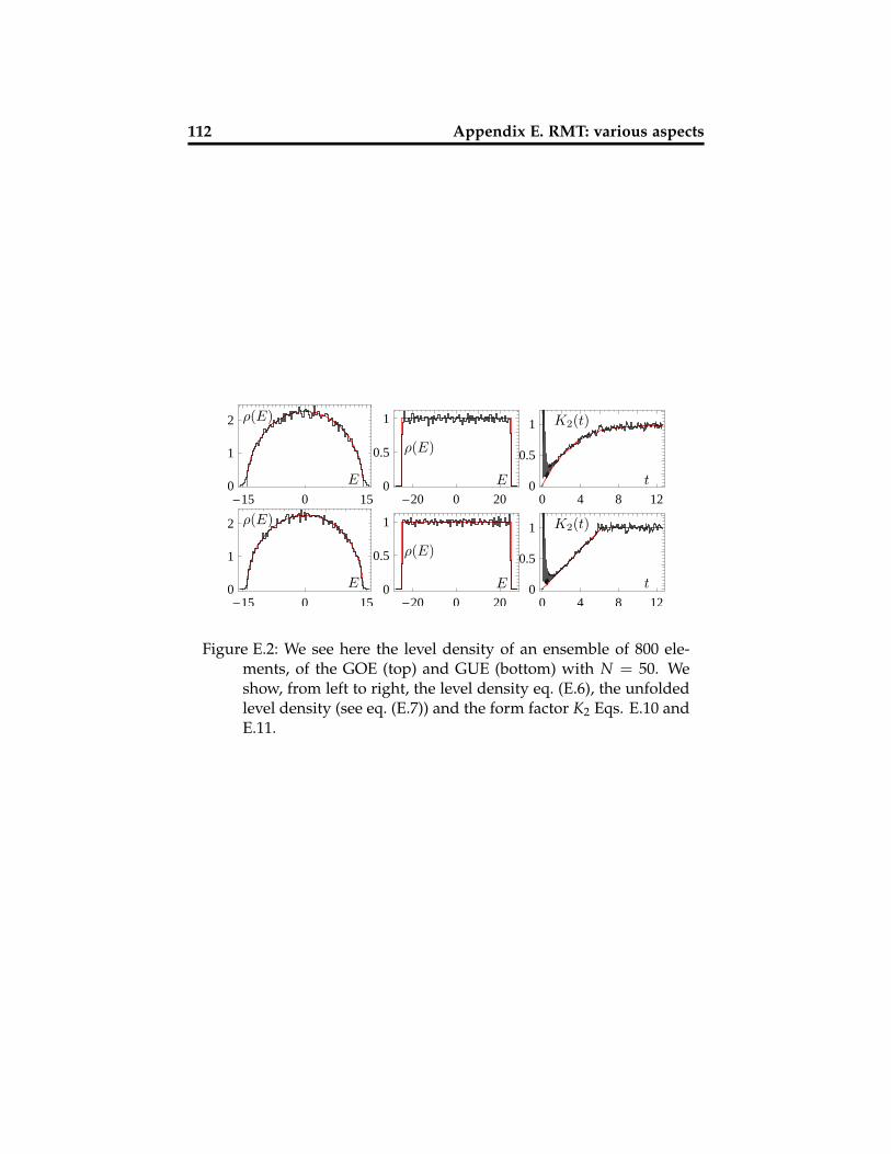
112 Appendix E. RMT: various aspects
-15 0 150
2
1
ρ(E)
E
-20 0 200
0.5
1
ρ(E)
E
0 4 8 120
0.5
1 K2(t)
t
-15 0 150
2
1
ρ(E)
E
-20 0 200
0.5
1
ρ(E)
E
0 4 8 120
0.5
1 K2(t)
t
Figure E.2: We see here the level density of an ensemble of 800 ele-ments, of the GOE (top) and GUE (bottom) with N = 50. Weshow, from left to right, the level density eq. (E.6), the unfoldedlevel density (see eq. (E.7)) and the form factor K2 Eqs. E.10 andE.11.

Appendix F
On the numerics of RMT andquantum information
We now describe some tricks to implement some aspects of RMT. We alsoinclude some of the routines useful for quantum information simulation.All routines are for Fortran 90. pi = π and I = ı.
F.1 Random matrices
To build the random matrices, as noted in Appendix E, one can use ran-dom Gaussian variables. Most low level languages provide homogeneousdistributions in the unit interval [0, 1). A transformation from this dis-tribution (characterizing variables u and v), to a complex Gaussian one(characterizing variable z) of width σ and centered at x0 is provided by
z = σe2πıv√−2 log u + x0 (F.1)
Its implementation is straightforward, however if u = 0 (which occurs nu-merically with very small, but finite probability) the routine could crash.If instead of selecting u ∈ [0, 1) we select 1− u ∈ [0, 1), the problem isfixed. The routine is called RandomGaussian. Its first argument is σ andthe second one x0.
In view of the considerations of the Appendix E, to build a GUE matrix,one has to choose the diagonal elements real and with σ2 = 1 whereas for
113
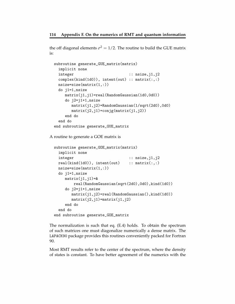
114 Appendix F. On the numerics of RMT and quantum information
the off diagonal elements σ2 = 1/2. The routine to build the GUE matrixis:
subroutine generate_GUE_matrix(matrix)implicit noneinteger :: nsize,j1,j2complex(kind(1d0)), intent(out) :: matrix(:,:)nsize=size(matrix(1,:))do j1=1,nsize
matrix(j1,j1)=real(RandomGaussian(1d0,0d0))do j2=j1+1,nsize
matrix(j1,j2)=RandomGaussian(1/sqrt(2d0),0d0)matrix(j2,j1)=conjg(matrix(j1,j2))
end doend do
end subroutine generate_GUE_matrix
A routine to generate a GOE matrix is
subroutine generate_GOE_matrix(matrix)implicit noneinteger :: nsize,j1,j2real(kind(1d0)), intent(out) :: matrix(:,:)nsize=size(matrix(1,:))do j1=1,nsize
matrix(j1,j1)=&real(RandomGaussian(sqrt(2d0),0d0),kind(1d0))
do j2=j1+1,nsizematrix(j1,j2)=real(RandomGaussian(),kind(1d0))matrix(j2,j1)=matrix(j1,j2)
end doend do
end subroutine generate_GOE_matrix
The normalization is such that eq. (E.4) holds. To obtain the spectrumof such matrices one must diagonalize numerically a dense matrix. TheLAPACK90 package provides this routines conveniently packed for Fortran90.
Most RMT results refer to the center of the spectrum, where the densityof states is constant. To have better agreement of the numerics with the

F.2. Quantum information 115
theory one can unfold the spectrum, i.e. force an approximate constantlevel density. Given a density ρ(E), the function η(e) =
∫ emin{E} dEρ(E)
maps E to an “unfolded” energy e. Since∫ e
−1
2Nπ
√1− E2 =
Nπ
(e√
1− e2 + π − sin−2 e)
(F.2)
(which would assume an spectrum with ranging roughly from ±1), thefollowing routine gives an unfolded spectrum, ranging from 0 to N.
function approxcumulative(Energy,size_spectrum)real(kind(1d0)) :: approxcumulativereal(kind(1d0)), intent(in) :: energyinteger, intent(in) :: size_spectrumreal(kind(1d0)) :: rescaled_energyrescaled_energy=Energy*sqrt(pi)/size_spectrumif (rescaled_energy <= -1D0) approxcumulative=0d0if (rescaled_energy >= 1D0) approxcumulative=piif ((-1d0<rescaled_energy).and.(rescaled_energy<1d0)) &
approxcumulative=(asin(rescaled_energy)+ &rescaled_energy*sqrt(1-rescaled_energy**2)+pi/2)approxcumulative=(approxcumulative-pi/2)*size_spectrum/pi
end function approxcumulative
We assume in this function that the spectrum ranges from ±N/√
π.The unfolding procedure can also work with the same routine presentedabove as the level density is again a semicircle.
F.2 Quantum information
During the numerical implementation of the ideas exposed in the the-sis, we have to do operations that involve tensor product of states [as ineq. (2.4)], like
|ψ〉 = |ψA〉 ⊗ |ψB〉 (F.3)
with |ψA〉 ∈ HA and |ψB〉 ∈ HB. We shall assume that both HA and HBare spaces of one or more qubits. This allows to take advantage of thebitwise operations available in all programing languages.
In order to explain the implementation of tensor products its better touse an example. We restrict our selfs to tensor products of qubit spaces.

116 Appendix F. On the numerics of RMT and quantum information
Consider an space composed of L qubits, numbered from 0 to L − 1:H = HL−1 ⊗ · · · ⊗ H0. Now consider the two subspaces HA = HaA−1 ⊗· · · ⊗ Ha0 of dimension 2A and HB = HbB−1 ⊗ · · · ⊗ Hb0 of dimension2B such that H = HA ⊗ HB. Assume that L = 7, HA is the subspaceof qubits 0, 3 and 5 and thus HB is the subspace of qubits 1, 2, 4, 6.One can label unambiguously HA with a number nA = ∑i 2ai . In ourcase, na = 20 + 23 + 25 = 41. Analogously one can label HB with nb =21 + 22 + 24 + 26 = 86 (notice that na + nb = 2L − 1 and thus are notindependent). Using tensor notation, one can associate an single index µof H with two indices, one in HA and one in HB. If one uses the notationexplained in Appendix B one must combine the binary bits of index µwith the bits of the numbers representing each space (say iA in HA andiB in HB) . As an example assume that µ = 55. One obtains na = 5 andnb = 7, as shows the following table.
qubit number 6 5 4 3 2 1 0µ = 55 0 1 1 0 1 1 1na = 41 0 1 0 1 0 0 1iA = 5 1 0 1
nb = 86 1 0 1 0 1 1 0iB = 7 0 1 1 1
A routine implementing the procedure is
subroutine exdig(number_in,L,n1out,n2out,nwhich)implicit noneinteger, intent(in) :: L,nwhich,number_ininteger, intent(out) :: n1out,n2outinteger :: j,numin, L1,L2n1out=0n2out=0numin=number_inL1=bits_on_one(nwhich)L2=L-L1do j=0,L-1
if (btest(nwhich,j)) thenif (btest(numin,0)) n1out=ibset(n1out,0)n1out=ishftc(n1out,-1,L1)
elseif (btest(numin,0)) n2out=ibset(n2out,0)

F.2. Quantum information 117
n2out=ishftc(n2out,-1,L2)endifnumin=ishftc(numin,-1,L)
end doreturn
end subroutine exdig
Here number in = µ, L = L, n1out = iA , n2out = iB, and nwhich = na. Aroutine to calculate tensor products of real matrices, that takes advantageof the previous routine is the following.
subroutine TensorProduct_real_routine(H_a,H_b,nwhich,H_out)integer, intent(in) :: nwhichreal(kind(1d0)), intent(in) :: H_a(0:,0:),H_b(0:,0:)real(kind(1d0)), intent(out):: H_out(0:,0:)integer :: total_size, j1, j2, &
j1a, j1b, j2a, j2b, qubitstotal_size=size(H_a,1)*size(H_b,1)qubits=IntegerLogBase2(total_size)do j1=0,total_size-1
do j2=0,total_size-1call exdig(j1,qubits,j1a,j1b,nwhich)call exdig(j2,qubits,j2a,j2b,nwhich)H_out(j1,j2)=H_a(j1a,j2a)*H_b(j1b,j2b)
enddoenddo
The function IntegerLogBase2 calculates the integer logarithm in base 2,of its argument (it must be a power of 2). Again nwhich = na, H A (H B) isthe operator acting in HA (HA).
The last routine that we wish to document is one for performing partialtraces. This routine calculates the partial trace over HB of a pure stateρ = trB |ψ〉〈ψ|. The input parameters are the state |ψ〉 (statin) and na(nwhich). The output parameter rho is ρ.
subroutine safe_PartialTrace(statin,rho,nwhich)implicit nonecomplex(kind(1d0)) :: statin(:)complex(kind(1d0)) :: rho(0:,0:)
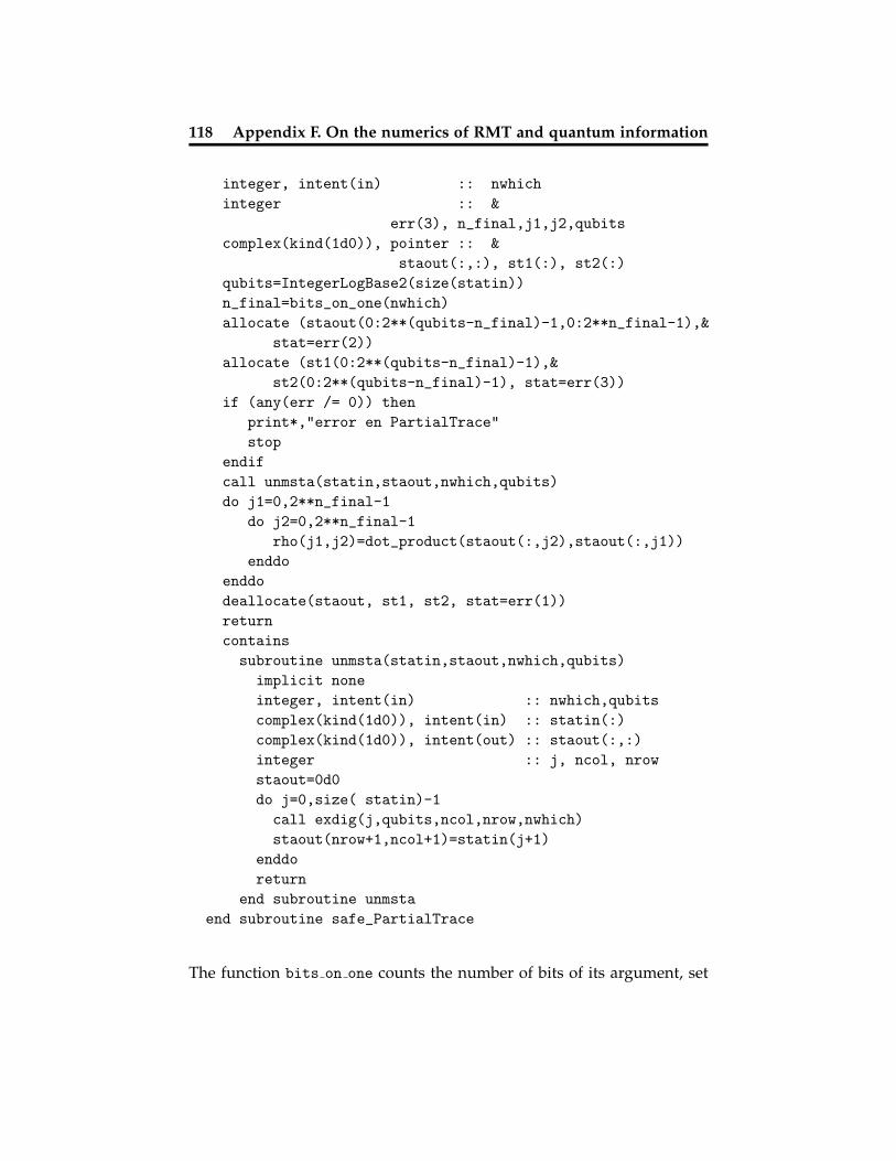
118 Appendix F. On the numerics of RMT and quantum information
integer, intent(in) :: nwhichinteger :: &
err(3), n_final,j1,j2,qubitscomplex(kind(1d0)), pointer :: &
staout(:,:), st1(:), st2(:)qubits=IntegerLogBase2(size(statin))n_final=bits_on_one(nwhich)allocate (staout(0:2**(qubits-n_final)-1,0:2**n_final-1),&
stat=err(2))allocate (st1(0:2**(qubits-n_final)-1),&
st2(0:2**(qubits-n_final)-1), stat=err(3))if (any(err /= 0)) then
print*,"error en PartialTrace"stop
endifcall unmsta(statin,staout,nwhich,qubits)do j1=0,2**n_final-1
do j2=0,2**n_final-1rho(j1,j2)=dot_product(staout(:,j2),staout(:,j1))
enddoenddodeallocate(staout, st1, st2, stat=err(1))returncontainssubroutine unmsta(statin,staout,nwhich,qubits)implicit noneinteger, intent(in) :: nwhich,qubitscomplex(kind(1d0)), intent(in) :: statin(:)complex(kind(1d0)), intent(out) :: staout(:,:)integer :: j, ncol, nrowstaout=0d0do j=0,size( statin)-1
call exdig(j,qubits,ncol,nrow,nwhich)staout(nrow+1,ncol+1)=statin(j+1)
enddoreturn
end subroutine unmstaend subroutine safe_PartialTrace
The function bits on one counts the number of bits of its argument, set

F.2. Quantum information 119
to 1. The subroutine unmsta reorganizes the input state as a matrix, to beable to express the partial trace as a dot product of the vectors composingthis matrix. All the programs, and routines are available upon explicitrequest to the author.

Appendix G
Two minor technicalities
G.1 The Form Factor
We define the spectral form factor as
K(t) =1N
N
∑i=1
eıtEi . (G.1)
Some authors rescale the energy (or, equivalently the time). The factor infront is used to obtain an asymptotic average value of one for most spec-tra. This quantity has been studied extensively in the context of quantumchaos [GMGW98, JPA]
We want to evaluate a double integral of the two-level form factor for theGUE case:
Bβ=22 (t) :=
∫ t
0dτ∫ τ
0dτ′bβ=2
2
(τ′ − τ
τH
)=∫ t
0dτ∫ τ
0dτ′b2
2
(τ′
τH
)(G.2)
Let us suppose first that 0 < t < τH, and thus replace b22 by a linear
expression:
B22(t) =
∫ t
0dτ∫ τ
0dτ′bβ=2
2
(τ′ − τ
τH
)(G.3)
=∫ t
0dτ∫ τ
0dτ′
(1− τ′
τH
)(G.4)
=t2
2− t3
6τH. (G.5)
121

122 Appendix G. Two minor technicalities
If t > τH the expression must be strictly linear since b22(t ≥ τH) = 0, and
with slope given by∫ τH
0 b22(t/τH) = τH/2. Furthermore, since B2
2(t) mustbe continuous, we also have the y intersect of the linear function. Thisleave us with the result
B22(t) =
t2
2 − t3
6τHif 0 ≤ t < τH
tτH2 −
τ2H6 if t ≥ τH
. (G.6)
G.2 A small proof of the Born expansion
Consider the Hamiltonian Hλ = H0 + λW. The definition of the state ketin the interaction picture is [Sak94]
|ψ(t)〉I = U†0 (t)Uλ(t)|ψ(0)〉 (G.7)
where Uλ(t) = exp(ıtHλ). Consider the equation of motion of the ket inthe interaction picture [Sak94]:
ıd|ψ(t)〉I
dt= λW|ψ(t)〉I (G.8)
with W(t) = U†0 (t)WU0(t). Formal integration leads to
|ψ(t)〉I = |ψ(0)〉 − ıλ∫ t
0dτW(τ)|ψ(τ)〉I . (G.9)
Solving the integral by iteration we obtain
|ψ(t)〉I =(11 + (−ıλ)
∫ t
0dτW(τ) + (−ıλ)2
∫ t
0dτ∫ τ
0dτ′W(τ′) + . . .
)|ψ(0)〉.
(G.10)
Comparing (G.7) and (G.10) we obtain the Born expansion:
U†0 (t)Uλ(t) = 11 + (−ıλ)
∫ t
0dτW(τ)
+ (−ıλ)2∫ t
0dτ∫ τ
0dτ′W(τ)W(τ′) + · · · . (G.11)

Bibliography
[Alb92] A. Albrecht. Investigating decoherence in a simple system.Phys. Rev. D, 46(12):5504–5520, Dec 1992.
[Alb93] A. Albrecht. Following a ”collapsing” wave function. Phys.Rev. D, 48(8):3768–3778, Oct 1993.
[ALKH02] D. Ahn, J. Lee, M. S. Kim, and S. W. Hwang. Self-consistent non-markovian theory of a quantum-state evo-lution for quantum-information processing. Phys. Rev. A,66(1):012302, Jul 2002.
[AV07] R. F. Abreu and R. O. Vallejos. Statistical bounds on thedynamical production of entanglement. March 2007, quant-ph/0703057.
[Bal68] R. Balian. Random matrices and information theory. IlNuovo Cimento B, (57):183, 1968.
[BBC+93] C. H. Bennett, G. Brassard, C. Crepeau, R. Jozsa, A. Peres,and W. K. Wootters. Teleporting an unknown quantumstate via dual classical and einstein-podolsky-rosen chan-nels. Phys. Rev. Lett., 70(13):1895–1899, Mar 1993.
[BFF+81] T. A. Brody, J. Flores, J. B. French, P. A. Mello, A. Pandey,and S. S. M. Wong. Random matrix physics: Spectrum andstrength fluctuations. Rev. Mod. Phys., 53:385–479, 1981.
[BGdS95] O. Bohigas, M.-J. Giannoni, A. M. O. de Almeida, andC. Schmit. Chaotic dynamics and the GOE-GUE transition. Nonlinearity, 8:203–221, March 1995.
[BGS84] O. Bohigas, M. J. Giannoni, and C. Schmit. Characteriza-tion of chaotic quantum spectra and universality of levelfluctuation laws. Phys. Rev. Lett., 52(1):1–4, Jan 1984.
123
124 BIBLIOGRAPHY
[BMM05] J. P. Barjaktarevic, G. J. Milburn, and Ross H. McKenzie.Fast simulation of a quantum phase transition in an ion-trap realizable unitary map. Phys. Rev. A, 71(1):012335, 2005.
[Bra06] D. Braun. Decoherence in a system of many two-levelatoms. Phys. Rev. Lett., 96(23):230502, 2006.
[Bro73] T. A. Brody. Lett. Nuovo Cimento, 7:482, 1973.
[Car35] E. Cartan. Quasi composition algebras. Abh. Math. Sem.Hamburg, 11:116, 1935.
[CDPZ03] F. M. Cucchietti, D. A. R. Dalvit, J. P. Paz, and W. H.Zurek. Decoherence and the Loschmidt Echo. Phys. Rev.Lett., 91(21):210403, 2003.
[CdRF+05] C. W. Chou, H. de Riedmatten, D. Felinto, S. V. Polyakov,S. J. van Enk, and H. J. Kimble. Measurement-induced en-tanglement for excitation stored in remote atomic ensem-bles. Nature, 438:828–832, Dec 2005.
[CGVG80] G. Casati, I. Guarneri, and F. Valz-Gris. On the connectionbetween quantization of nonintegrable systems and statis-tical theory of spectra. Lett. Nuovo Cimento Soc. Ital. Fis.,28:279, 1980.
[CL83] A. O. Caldeira and A. J. Leggett. Path integral approachto quantum Brownian motion. Physica A, 121:587–616,September 1983.
[CMJ+05] T. Chaneliere, D. N. Matsukevich, S. D. Jenkins, S. Y. Lan,T. A. B. Kennedy, and A. Kuzmich. Storage and retrieval ofsingle photons transmitted between remote quantum mem-ories. Nature, 438:833–836, Dec 2005.
[CPW02] F. M. Cucchietti, H. M. Pastawski, and D. A. Wisniacki. De-coherence as decay of the Loschmidt echo in a Lorentz gas.Phys. Rev. E, 65(4):045206, 2002.
[CPZ05] G. L. Celardo, C. Pineda, and M. Znidaric. Stability of quan-tum Fourier transformation on Ising quantum computer.Int. J. Quantum Inf., 3(3):441, 2005, quant-ph/0310163.
[DDG+03] C. Dembowski, B. Dietz, H.-D. Graf, A. Heine, F. Leyvraz,M. Miski-Oglu, A. Richter, and T. H. Seligman. Phase ShiftExperiments Identifying Kramers Doublets in a ChaoticSuperconducting Microwave Billiard of Threefold Sym-
BIBLIOGRAPHY 125
metry. Phys. Rev. Lett., 90(1):014102–+, January 2003,arXiv:nlin/0211033.
[DDZ00] D. A. R. Dalvit, J. Dziarmaga, and W. H. Zurek. Deco-herence in bose-einstein condensates: Towards bigger andbetter schrodinger cats. Phys. Rev. A, 62(1):013607, Jun 2000.
[DRS91] F.-M. Dittes, I. Rotter, and T. H. Seligman. Chaotic be-haviour of scattering induced by strong external coupling.Phys. Lett. A, 158:14–18, August 1991.
[dSDS03a] R. de Sousa and S. Das Sarma. Electron spin coher-ence in semiconductors: considerations for a spin-basedsolid-state quantum computer architecture. Phys. Rev. B,67(3):033301, Jan 2003.
[dSDS03b] R. de Sousa and S. Das Sarma. Theory of nuclear-inducedspectral diffusion: Spin decoherence of phosphorus donorsin si and gaas quantum dots. Phys. Rev. B, 68(11):115322,Sep 2003.
[Dys62] F. J. Dyson. A Brownian-motion model for the eigenvaluesof a random matrix. J. Math. Phys., 3(6):1191–1198, Novem-ber/December 1962.
[EAM+05] M. D. Eisaman, A. Andre, F. Massou, M. Fleischhauer,A. S. Zibrov, and M. D. Lukin. Electromagnetically inducedtransparency with tunable single-photon pulses. Nature,438:837–841, Dec 2005.
[ELPC04] J. Emerson, S. Lloyd, D. Poulin, and D. Cory. Estimation ofthe local density of states on a quantum computer. Phys.Rev. A, 69(5):050305, 2004.
[Eve57] H. Everett. ”Relative State” formulation of quantum me-chanics. Rev. Mod. Phys., 29(3):454–462, Jul 1957.
[EWS+03] J. Emerson, Y. S. Weinstein, M. Saraceno, S. Lloyd, and D. G.Cory. Pseudo-Random Unitary Operators for Quantum In-formation Processing. Science, 302(5653):2098–2100, 2003.
[FFP04] L. Fedichkin, A. Fedorov, and V. Privman. Additivity of de-coherence measures for multiqubit quantum systems. Phys.Lett. A, 328:87–93, Jul 2004.
[FFS04] K. M. Frahm, R. Fleckinger, and D. L. Shepelyansky. Quan-tum chaos and random matrix theory for fidelity decay
126 BIBLIOGRAPHY
in quantum computations with static imperfections. Eur.Phys. J. D, 29:139–155, 2004, quant-ph/0312120.
[Ged06] Z. Gedik. Spin bath decoherence of quantum entanglement.Solid State Commun., 138:82, 2006.
[GKP+06] T. Gorin, H. Kohler, T. Prosen, T. H. Seligman, H.-J.Stockmann, and M. Znidaric. Anomalous slow fidelity de-cay for symmetry-breaking perturbations. Phys. Rev. Lett.,96(24):244105, 2006.
[GLM04] V. Giovannetti, S. Lloyd, and L. Maccone. Quantum-Enhanced Measurements: Beating the Standard QuantumLimit. Science, 306(5700):1330–1336, 2004.
[GLM06] V. Giovannetti, S. Lloyd, and L. Maccone. Quantum metrol-ogy. Phys. Rev. Lett., 96(1):010401, 2006.
[GMCMB07] I. Garcia-Mata, A. R. R. Carvalho, F. Mintert, and A. Buch-leitner. Entanglement screening by nonlinear resonances.Phys. Rev. Lett., 98(12):120504, 2007.
[GMGW98] T. Guhr, A. Muller-Groeling, and H. A. Weidenmuller.Random matrix theories in quantum physics: Commonconcepts. Phys. Rep., 299(4):189–425, June 1998, cond-mat/9707301.
[GPS04] T. Gorin, T. Prosen, and T. H. Seligman. A random matrixformulation of fidelity decay. New J. Phys., 6:20, 2004.
[GPS07] T. Gorin, C. Pineda, and T. H. Seligman. Decoherence ofan n-qubit quantum memory. 2007, quant-ph/0703190. Ac-cepted in Phys. Rev. Lett.
[GPSS04] T. Gorin, T. Prosen, T. H. Seligman, and W. T. Strunz. Con-nection between decoherence and fidelity decay in echo dy-namics. Phys. Rev. A, 70(4):042105, 2004.
[GPSZ06] T. Gorin, T. Prosen, T. H. Seligman, and M. Znidaric. Dy-namics of Loschmidt echoes and fidelity decay. Phys. Rep.,435:33, 2006, quant-ph/0607050.
[GS02] T. Gorin and T. H. Seligman. A random matrix approach todecoherence. J. Opt. B, 4(4):S386, 2002.
[GS03] T. Gorin and T. H. Seligman. Decoherence in chaotic andintegrable systems: a random matrix approach. Phys. Lett.

BIBLIOGRAPHY 127
A, 309:61–67, Mar 2003.
[GSW06] T. Gorin, T. H. Seligman, and R. L. Weaver. Scattering fi-delity in elastodynamics. Phys. Rev. E, 73(1):015202(R), 2006.
[Haa01] F. Haake. Quantum Signatures of Chaos, II ed. Springer,Berlin, 2001.
[HHR+05] H. Haffner, W. Hansel, C. F. Roos, J. Benhelm, D. Chek-al-kar, M. Chwalla, T. Korber, U. D. Rapol, M. Riebe, P. O.Schmidt, C. Becher, O. Guhne, W. Dur, and R. Blatt. Scal-able multiparticle entanglement of trapped ions. Nature,438:643, December 2005, quant-ph/0603217.
[HSKH+05] H. Haffner, F. Schmidt-Kaler, W. Hansel, C. F. Roos,T. Korber, M. Chwalla, M. Riebe, J. Benhelm, U. D. Rapol,C. Becher, and R. Blatt. Robust entanglement. AppliedPhysics B: Lasers and Optics, 81:151, Jul 2005.
[HW97] S. Hill and W. K. Wootters. Entanglement of a pair of quan-tum bits. Phys. Rev. Lett., 78(26):5022, 1997.
[JL03] R. Jozsa and N. Linden. On the role of entanglement inquantum computational speed-up. Proc. R. Soc. London, Ser.A, 459:2011–2032, June 2003.
[JPA] J. Phys A 36 No. 12 (2003).
[JSC+04] B. Julsgaard, J. Sherson, J. I. Cirac, J. Fiurasek, and E. S.Polzik. Experimental demonstration of quantum memoryfor light. Nature, 432:482–486, Nov 2004.
[KA06] O. Kern and G. Alber. Selective recoupling and stochasticdynamical decoupling. Phys. Rev. A, 73(6):062302, 2006.
[KAS05] O. Kern, G. Alber, and D. L. Shepelyansky. Quantum errorcorrection of coherent errors by randomization. The Euro-pean Physical Journal D - Atomic, Molecular, Optical and PlasmaPhysics, 32:153–156, Jan 2005. 10.1140/epjd/e2004-00196-9.
[KD98] A. Kramer and S. Doniach. Superinsulator phase of two-dimensional superconductors. Phys. Rev. Lett., 81(16):3523–3526, Oct 1998.
[Key02] M. Keyl. Fundamentals of quantum information theory.Phys. Rev., 369:431–548, Oct 2002.
[KJZ02] Z. P. Karkuszewski, C. Jarzynski, and W. H. Zurek. Quan-
128 BIBLIOGRAPHY
tum chaotic environments, the butterfly effect, and deco-herence. Phys. Rev. Lett., 89(17):170405, Oct 2002.
[KS04] H. G. Krojanski and D. Suter. Scaling of decoherence inwide nmr quantum registers. Phys. Rev. Lett., 93(9):090501,2004.
[KS06] H. G. Krojanski and D. Suter. Decoherence in large nmrquantum registers. Phys. Rev. A, 74(6):062319, 2006.
[LDK+05] J. Lages, V. V. Dobrovitski, M. I. Katsnelson, H. A. De Raedt,and B. N. Harmon. Decoherence by a chaotic many-spinbath. Phys. Rev. E, 72(2):026225, 2005.
[LKA+04] J. Lee, I. Kim, D. Ahn, H. McAneney, and M. S. Kim. Com-pletely positive non-markovian decoherence. Phys. Rev. A,70(2):024301, 2004.
[LS05] A. Lakshminarayan and V. Subrahmanyam. Multipartiteentanglement in a one-dimensional time-dependent isingmodel. Phys. Rev. A, 71(6):062334, 2005.
[MCKB05] F. Mintert, A. R. R. Carvalho, M. Kus, and Andres. Buch-leitner. Measures and dynamics of entangled states. Phys.Rep., 415(4):207, 2005.
[Meh91] M. L. Mehta. Random Matrices. Academic Press, San Diego,California, second edition, 1991.
[Mel95] P. A. Mello. Theory of random matrices: spectral statisticsand scattering problems in mesoscopic quantum physics.In E. Akkermans, G. Montambaux, and J.-L Pichard, edi-tors, Mesoscopic Quantum Physics. Elsevier Science B.V., Am-sterdam, 1995. Proceedings of the Les Houches SummerSchool, Session LXI.
[MJWK01] W. J. Munro, D. F. V. James, A. G. White, and P. G. Kwiat.Maximizing the entanglement of two mixed qubits. Phys.Rev. A, 64(3):030302, 2001.
[MPK88] P. A. Mello, P. Pereyra, and N. Kumar. A soluble random-matrix model for relaxation in quantum systems. J. Stat.Phys., 51:77–94, Apr 1988. 10.1007/BF01015321.
[NC00] M. A. Nielsen and I. L. Chuang. Quantum Computation andQuantum Information. Cambridge University Press, Cam-bridge, U.K., 2000.
BIBLIOGRAPHY 129
[PF02] T. B. Pittman and J. D. Franson. Cyclical quantum memoryfor photonic qubits. Phys. Rev. A, 66(6):062302, Dec 2002.
[PFL+04] A. Poppe, A. Fedrizzi, T. Loruenser, O. Maurhardt, R. Ursin,H. R. Boehm, M. Peev, M. Suda, C. Kurtsiefer, H. Wein-furter, T. Jennewein, and A. Zeilinger. Practical QuantumKey Distribution with Polarization-Entangled Photons. Op-tics Express, 12(16):3865–3871, 2004, quant-ph/0404115.
[PGS07] C. Pineda, T. Gorin, and T. H. Seligman. Decoherence oftwo-qubit systems: a random matrix description. New J.Phys., 9(4):106, April 2007, quant-ph/0702161.
[PP07] C. Pineda and T. Prosen. Non-universal level statisticsin a chaotic quantum spin chain. February 2007, quant-ph/0702164. Accepted in Phys. Rev. E.
[Pro00] T. Prosen. Exact time-correlation functions of quantumising chain in a kicking transversal magnetic field. Prog.Theor. Phys. Suppl., 139:191–203, 2000.
[Pro02] T. Prosen. General relation between quantum ergodic-ity and fidelity of quantum dynamics. Phys. Rev. E,65(3):036208, 2002.
[PS02] T. Prosen and T. H Seligman. Decoherence of spin echoes.J. Phys. A, 35(22):4707, 2002.
[PS06] C. Pineda and T. H. Seligman. Evolution of pairwise en-tanglement in a coupled n-body system. Phys. Rev. A,73(1):012305, 2006.
[PS07] C. Pineda and T. H. Seligman. Bell pair in a generic randommatrix environment. Phys. Rev. A, 75(1):012106, 2007.
[PSPS06] C. Pineda, R. Schafer, T. Prosen, and T. H. Seligman. Veri-fication of generic fidelity recovery in a dynamical system.Phys. Rev. E, 73(6):066120, 2006.
[PSW01] T. Prosen, T. H. Seligman, and H. A. Weidenmuller. Ran-dom matrix ensembles for semi-separable systems. Euro-phys. Lett., 55(1):12–18, 2001.
[PSZ03] T. Prosen, T. H. Seligman, and M. Znidaric. Estimationof purity in terms of correlation functions. Phys. Rev. A,67(6):062108, 2003.
130 BIBLIOGRAPHY
[PV07] M. B. Plenio and S. Virmani. An introduction to entangle-ment measures. Quant. Inf. Comp., 7:1, 2007.
[PZ01] T. Prosen and M. Znidaric. Can quantum chaos enhance thestability of quantum computation? J. Phys. A, 34(47):L681–L687, 2001.
[PZ02] T. Prosen and Marko Znidaric. Stability of quantum motionand correlation decay. J. Phys. A, 35(6):1455, 2002.
[Sak94] J. J. Sakurai. Modern Quantum Mechanics. Addison-WesleyPublishing Company, Reading, MA, Revised edition, 1994.
[SAOO95] Paul So, Steven M. Anlage, Edward Ott, and Robert N.Oerter. Wave chaos experiments with and without time re-versal symmetry: Gue and goe statistics. Phys. Rev. Lett.,74(14):2662–2665, Apr 1995.
[Sch07] Erhard Schmidt. Zur theorie der linearen und nichtlin-earen integralgleichungen. Math. Ann., 63:433–476, Dec1907. 10.1007/BF01449770.
[SGSS05] R. Schafer, T. Gorin, T. H. Seligman, and H.-J. Stockmann.Fidelity amplitude of the scattering matrix in microwavecavities. New J. Phys., 7:152, 2005.
[Sha48] C. E. Shannon. A mathematical theory of communication.The Bell System Technical Journal, 27:379–423, 623–656, july,october 1948.
[SKK+00] C. A. Sackett, D. Kielpinski, B. E. King, C. Langer, V. Meyer,C. J. Myatt, M. Rowe, Q. A. Turchette, W. M. Itano, D. J.Wineland, and C. Monroe. Experimental entanglement offour particles. Nature, 404:256, Mar 2000.
[SLH+04] R. W. Simmonds, K. M. Lang, D. A. Hite, S. Nam, D. P.Pappas, and J. M. Martinis. Decoherence in Josephsonphase qubits from junction resonators. Phys. Rev. Lett.,93(7):077003, 2004.
[SS05] H.-J. Stockmann and R. Schafer. Fidelity recovery in chaoticsystems and the Debye-Waller factor. Phys. Rev. Lett.,94(24):244101, June 2005.
[SSGS05] R. Schafer, H.-J. Stockmann, T. Gorin, and T. H. Selig-man. Experimental verification of fidelity decay: Fromperturbative to Fermi golden rule regime. Phys. Rev. Lett.,
BIBLIOGRAPHY 131
95(18):184102, 2005.
[ste] S. Mossmann, private communication, 2007.
[VADM01] F. Verstraete, K. Audenaert, J. Dehaene, and B. De Moor. Acomparison of the entanglement measures negativity andconcurrence. J. Phys. A, 34(47):10327–10332, 2001.
[vN55] J. von Neumann. Mathematical Foundations of Quantum Me-chanics. Princeton University Press, 1955.
[WFL02] T. J. Walls, T. V. Filippov, and K. K. Likharev. Quantumfluctuations in Josephson junction comparators. Phys. Rev.Lett., 89(21):217004, Nov 2002.
[Wig51] E. P. Wigner. On a class of analytic functions from the quan-tum theory of collisions. Ann. Math., 53:36, 1951.
[Wig55] E. P. Wigner. Characteristic vectors of bordered matriceswith infinite dimensions. Ann. Math., 62:548, 1955.
[Wis28] J. Wishart. The generalized product moment distribution insamples from a normal multivariate population. Biometrika,A20:32–52, 1928.
[WNG+03] T.-C. Wei, K. Nemoto, P. M. Goldbart, P. G. Kwiat, W. J.Munro, and F. Verstraete. Maximal entanglement versus en-tropy for mixed quantum states. Phys. Rev. A, 67(2):022110,2003.
[YE02] T. Yu and J. H. Eberly. Phonon decoherence of quantumentanglement: Robust and fragile states. Phys. Rev. B,66(19):193306, 2002.
[YE03] T. Yu and J. H. Eberly. Qubit disentanglement and decoher-ence via dephasing. Phys. Rev. B, 68(16):165322, Oct 2003.
[YE04] T. Yu and J. H. Eberly. Finite-time disentanglement viaspontaneous emission. Phys. Rev. Lett., 93(14):140404, 2004.
[ZB05] M. Ziman and V. Buzek. Concurrence versus purity: Influ-ence of local channels on bell states of two qubits. Phys. Rev.A, 72(5):052325, 2005.
[ZCP+07] A. Zazunov, M. Creux, E. Paladino, A. Crepieux, andT. Martin. Detection of finite frequency current mo-ments with a dissipative resonant circuit. 2007, cond-mat/0702247.
132 BIBLIOGRAPHY
[ZCZ+04] Z. Zhao, Y.-A. Chen, A.-N. Zhang, T. Yang, H. J. Briegel,and J.-W. Pan. Experimental demonstration of five-photonentanglement and open-destination teleportation. Nature,430:54, Jul 2004.
[Zur91] W.H. Zurek. Decoherence and the transition from quantumto classical. Phys. Today, 44(10):36, 1991, quant-ph/0306072.
[Zur03] W. H. Zurek. Decoherence, einselection, and the quantumorigins of the classical. Rev. Mod. Phys., 75(3):715, May 2003.