ANDRE SHIGUEO YAMASHITA

DEVELOPMENT OF A MULTI-OBJECTIVE TUNING TECHNIQUE FOR

MODEL PREDICTIVE CONTROLLERS

São Paulo 2015

ANDRÉ SHIGUEO YAMASHITA

DEVELOPMENT OF A MULTI-OBJECTIVE TUNING TECHNIQUE FOR

MODEL PREDICTIVE CONTROLLERS

Tese apresentada à Escola Politécnica da

Universidade de São Paulo para obtenção

do título de Doutor em Engenharia

São Paulo

2015

ANDRÉ SHIGUEO YAMASHITA

DEVELOPMENT OF A MULTI-OBJECTIVE TUNING TECHNIQUE FOR

MODEL PREDICTIVE CONTROLLERS

Tese apresentada à Escola Politécnica da

Universidade de São Paulo para obtenção

do título de Doutor em Engenharia

Área de concentração: Engenharia

Química

Orientador: Prof. Dr. Darci Odloak

São Paulo

2015

Catalogação na publicação

Yamashita, André Shigueo Development of a multiobjective tuning technique for

model predictive controllers / A. S. Yamashita – versão corr. – São Paulo, 2015

163 p. Tese (Doutorado) – Escola Politécnica da

Universidade de São Paulo. Departamento de Engenharia Química.

1. Model predictive control tuning 2. Robust tuning 3.

Multi-objective optimization tuning I. Universidade de São Paulo. Escola Politécnica. Departamento de Engenharia Química II. t

Este exemplar foi revisado e alterado em relação à versão original, sob responsabilidade única do autor e com a anuência do seu orientador.

São Paulo, 12 de fevereiro de 2015 Assinatura do autor ___________________________________

Assinatura do orientador _______________________________

ACKNOWLEDGEMENTS

I would like to thank my advisor, Professor Darci Odloak, for the continuous support

provided since the college senior year and throughout the Direct Doctorate program.

He led a fresh graduate student towards what seemed a distant and blurred goal,

engraving the obligations, enjoyments and limitations of the academia. His life advice

will be treasured. Also, the suggestions by the qualification test committee to polish

this work; the continuous support provided by Dr. Antonio C. Zanin, Dr. Luz A.

Alvarez, Dr. Bruno Capron, Dr. Márcio Martins, the Ph.D students Bruno Santoro and

Aldo Hinojosa, and the other members of the Cenpes and CETAI research centers;

the undergraduate research program opportunities given by Professors Jorge Gut

and José Pires Camacho; are all appreciated.

My parents played an important role nurturing, educating and providing ever since I

was born, possibly the most important factor that allowed for the completion of this

step, and for me being who I am.

Ever since my sophomore year at college, crew has been one of my favorite hobbies.

Ricardo Linares, the CEPEUSP crew coach, Beto Nascimento, the SCCP crew

coach and all the crew members provided me a delightful and soothing activity that

helped balancing stress and anxiety.

Friends can make a difference in one’s life. I would like to thank Marco Fujii for being

like an older brother to me; Vinicius for showing that you do not need to take life too

seriously; Cassiano for the double sculls workouts and nutrition tips; Daniela for the

long-distance conversations and encouragement; Alexandre for never being on time;

Bruno for the plethora of inside jokes and the answers to the most unexpected

questions; Daniel for the surfing tips; my co-workers at the University for coping with,

according to them, ‘penguin-suitable’ air conditioning temperatures.

Relationships, on the other hand, are more fragile, demanding, and difficult to make

work, but they are definitely worth it; and given enough time, the lasting ones will

grow into strong and flexible bonds. I would like to thank Camila for a year full of ups

and downs, happy moments and priceless lessons.

ABSTRACT

Two multi-objective optimization based tuning techniques for Model Predictive

Control (MPC) were developed. Both take into account the sum of the squared errors

between closed-loop trajectories and reference responses based on pre-defined

goals as tuning objectives; one solves a lexicographic optimization to obtain an

optimum set of tuning parameters (LTT), whereas the other solves a compromise

optimization problem (CTT). The main advantages are an automated framework, and

straightforward goal definition, which are capable of taking into account a

specification on the process dynamics, a time-domain metrics, and of embedding the

control engineer’s knowledge into a reliable approach. A fluid catalytic cracking

tuning case study unveiled the goal definition flexibility of the LTT, with respect to

output tracking and variable coupling. A heavy oil fractionator in closed-loop with a

MPC case study compared both tuning techniques developed here, and it was

observed that the LTT in fact prioritizes the main objectives, whereas the CTT yields

an average solution, in terms of the tuning objectives. The CTT was compared to

another multi-objective tuning technique from the literature, in the tuning of a MPC

with input targets and output zone control in closed-loop with a crude distillation unit

model. The simulation results showed that the CTT allows for faster results,

regarding the computational time to compute the tuning parameters and there is no

need of a posteriori decisions to select the best non-dominated solution. Real MPC

applications are strongly hindered by model uncertainty. This limitation was

addressed by the extension of the tuning techniques to account for multi-plant model

uncertainty, thus obtaining optimum robustly tuned parameters for nominal

controllers, addressing the trade-off between robustness and performance. A

robustly tuned Infinite Horizon MPC (IHMPC) was compared to a Robust IHMPC, in

closed-loop with a C3/C4 splitter system model. It was observed in a simulation that

even though the latter yields better output responses, it is two orders of magnitude

slower than the former in online operation.

Keywords: Model Predictive Control tuning, multi-objective optimization tuning, robust

tuning

RESUMO

Neste trabalho foram desenvolvidas duas técnicas de sintonia para controladores

preditivos por modelo. Ambas visam minimizar a soma do erro quadrático entre

respostas do sistema em malha fechada e trajetórias de referência pré-definidas; a

primeira resolve um problema de otimização lexicográfica enquanto a segunda

resolve um problema de otimização de compromisso. As vantagens dos métodos

apresentados são: maior automatização, definição de objetivos de sintonia intuitiva

que considera especificações na dinâmica do processo, uma métrica no domínio do

tempo e é capaz de incluir o conhecimento do engenheiro de controle em uma

técnica de sintonia confiável. Um estudo de caso no sistema de craqueamento

catalítico ilustrou a flexibilidade de definição dos objetivos da técnica lexicográfica.

Um estudo de caso sobre uma coluna de fracionadora de óleo pesado em malha

fechada com um controlador preditivo por modelo comparou ambas as estratégias

de sintonia desenvolvidas aqui e pode-se concluir que a técnica lexicográfica dá

prioridade aos objetivos importantes enquanto a técnica de compromisso calcula

uma solução média, com respeito aos objetivos. A técnica de compromisso foi

comparada a um método de sintonia da literatura quanto a aplicação em um

controlador preditivo de horizonte infinito com targets para as entradas e controle por

faixas das saídas com uma coluna de destilação. Observou-se que a técnica

desenvolvida aqui é computacionalmente mais rápida e não requer a escolha de

uma solução não-dominada dentre um conjunto de soluções de Pareto. Aplicações

reais de controle preditivo são severamente afetadas por incerteza de modelo.

Estendeu-se as técnicas desenvolvidas aqui para considerar o caso de incerteza

multi-planta, calculando parâmetros de sintonia robustos para controladores

nominais, visando tratar o compromisso entre performance e estabilidade e robustez

da malha fechada. Um controlador preditivo de horizonte infinito foi sintonizado de

forma robusta e comparado com um controlador preditivo robusto em malha fechada

com um modelo de separadora C3/C4. Observou-se que este consegue controlar

melhor o processo, entretanto, tem um tempo de computação duas ordens de

grandeza maior que o controlador nominal, em operação on-line.

Palavras-chave: sintonia de controladores baseado em modelo, sintonia robusta,

sintonia por otimização multi-objetivo.

LIST OF ILLUSTRATIONS

Figure 2-1: Time domain performance metrics (MATLAB, 2013). ............................. 30

Figure 2-2: Tuning techniques classification chart. .................................................... 30

Figure 5-1: FCC schematic representation (Adapted from Grosdidier et al., 1993). .. 60

Figure 5-2: FCC reference trajectories, open-loop response (──), first-order

approximation ( ) and final reference trajectory ( ). ......................................... 62

Figure 5-3: Closed-loop output responses obtained in the first tuning step (──), last

tuning step ( ) and reference trajectory ( ). ...................................................... 64

Figure 5-4a: Evolution of output responses in the tuning of the FCC unit using the

goals defined in Scenario I, outputs. ......................................................................... 65

Figure 5-3b: Evolution of output responses in the tuning of the FCC unit using the

goals defined in Scenario I, inputs. ............................................................................ 65

Figure 5-4: FCC closed-loop responses resulting from tuning scenarios I (──) and

II ( ) and reference trajectories ( ). .................................................................. 67

Figure 5-5: Output tracking of the FCC unit simulation, Scenario I (──),

Scenario II ( ). Set points ( ). ........................................................................... 69

Figure 5-6: Inputs of the FCC unit simulation, Scenario I (──), Scenario II ( ). ... 70

Figure 5-7: Shell Heavy Oil Fractionator 3x3 subsystem schematic representation. . 72

Figure 5-8a: Responses of the HOF system outputs with LTT calculated in Step

1(──), Step 2 ( ) and Step 3 ( ) and reference trajectories ( ). ..................... 76

Figure 5-9b: Responses of the HOF system inputs with LTT calculated in Step 1(──),

Step 2 ( ) and Step 3 ( ). .................................................................................. 77

Figure 5-10: Simulation I. HOF outputs to set point changes ( ), LTT (──) and

CTT ( ). ................................................................................................................ 81

Figure 5-11: Simulation I. HOF inputs, LTT (──) and CTT ( ) and the upper

and lower bounds ( ). ............................................................................................ 82

Figure 5-12: Simulation II. HOF output to set point changes ( ) and unmeasured

disturbances, LTT (──) and CTT ( ). .............................................................. 83

Figure 5-13: Simulation II. HOF inputs, LTT (──) and CTT ( ) and the upper

and lower bounds ( ). ............................................................................................ 84

Figure 5-14: Schematic Representation of Crude Distillation Unit. ............................ 88

Figure 5-15a: Output tracking tuning analysis, CTT (──), NBI ( ),

existing controller ( ), Utopia ( ) ........................................................................ 95

Figure 5-15b: Output tracking tuning analysis, CTT (──), NBI ( ),

existing controller ( ), Utopia ( ) ........................................................................ 96

Figure 5-16a: Input tracking tuning analysis, CTT II-A ( ), CTT II-B (──), existing

controller ( ), reference trajectory ( ). .............................................................. 100

Figure 5-16b: Input tracking tuning analysis, CTT II-A ( ), CTT II-B (──), existing

controller ( ), reference trajectory ( ). .............................................................. 101

Figure 5-17: Outputs of the CDU in closed loop simulation with MPC tuned with

CTT II-B (──), NBI II-B ( ), existing controller ( ) and bounds ( ). .............. 105

Figure 5-18a: Inputs of the CDU in closed loop simulation with MPC tuned with

CTT II-B (──), NBI II-B ( ), existing controller ( ) and targets ( ). ............... 106

Figure 5-18b: Inputs of the CDU in closed loop simulation with MPC tuned with

CTT II-B (──), NBI II-B ( ), existing controller ( ) and targets ( ). ............... 107

Figure 5-18c: Inputs of the CDU in closed loop simulation with MPC tuned with

CTT II-B (──), NBI II-B ( ), existing controller ( ) and targets ( ). ............... 108

Figure 5-19: Schematic view of the C3/C4 splitter system, (Porfírio, Neto & Odloak,

2003). ...................................................................................................................... 109

Figure 5-20: C3/C4 splitter model-plant mismatch Simulation I, LTT IHMPC

responses ( ) and set points or bounds ( ). ...................................................... 111

Figure 5-21: C3/C4 splitter RLTT, output responses of the first step. ...................... 114

Figure 5-22: C3/C4 splitter RLTT, output responses of the second step. ................ 114

Figure 5-23: C3/C4 RCTT tuning results, outputs. .................................................. 116

Figure 5-24: Responses of the IHMPC tuned with RLTT (──), RCTT ( ) and

LTT ( ). Set points and input bounds ( ). .......................................................... 118

Figure 5-25: C3/C4 splitter Simulation I. IHMPC with RLTT (──), RCTT ( ) and a

RIHMPC ( ). Set points and input bounds ( ). .................................................. 119

Figure 5-26: C3/C4 splitter Simulation II. IHMPC with RLTT (──), IHMPC with

RCTT ( ), RIHMPC ( ). Set points ( ). ......................................................... 121

Figure 5-27: Simulation II from 1000 min to 1500 min. IHMPC with RLTT (──),

IHMPC with RCTT ( ), RIHMPC ( ). Set points ( ). ..................................... 122

LIST OF TABLES

Table 3-1: Lexicographic technique steps summary ................................................. 48

Table 5-1: FCC unit input and output list. .................................................................. 59

Table 5-2: FCC unit gain matrix considering normalized transfer functions............... 60

Table 5-3: FCC lexicographic tuning results, Scenario I. ........................................... 66

Table 5-4: Lexicographic tuning slack variables and cost function values, Scenario I.

.................................................................................................................................. 66

Table 5-5: Lexicographic tuning results, Scenario II. ................................................. 67

Table 5-6: Lexicographic slack variables and cost function values, Scenario II. ....... 67

Table 5-7: FCC simulation study, set point changes. ................................................ 68

Table 5-8: Parameters of the reference transfer function .......................................... 73

Table 5-9: Lexicographic optimum tuning parameters. .............................................. 75

Table 5-10: Lexicographic slack variables, δt. ........................................................... 75

Table 5-11: Optimum tuning parameters summary. .................................................. 79

Table 5-12: Simulation I set points. ........................................................................... 80

Table 5-13: Simulation II set points. .......................................................................... 80

Table 5-14: ISE index calculated for the simulation responses. ................................ 80

Table 5-15: CDU controlled outputs. ......................................................................... 89

Table 5-16: CDU manipulated inputs. ....................................................................... 89

Table 5-17: CDU input-output relationship matrix. ..................................................... 93

Table 5-18: Reference trajectories transfer function time constants. ......................... 93

Table 5-19: Tuning results for Scenario II-A and II-B. ............................................. 103

Table 5-20: Tuning strategies comparison. ............................................................. 103

Table 5-21: List of variables of the C3/C4 splitter system. ....................................... 109

Table 5-22: Set point changes of the C3/C4 Simulation I. ....................................... 110

Table 5-23: C3/C4 RCTT results, F° for each model. .............................................. 115

Table 5-24: C3/C4 Simulation II set points. ............................................................. 120

NOMENCLATURE

A State transition matrix

eqA Equality constraint coefficient matrix

inA Inequality constraint coefficient matrix

B States to system inputs relationship matrix

eqb Equality constraint independent vector

, ,i j kb k-th coefficient of the numerator of transfer function Gi,j(s)

inb Inequality constraint independent vector

C States to system outputs relation matrix

c QP constant term Tfc QP linear term vector

iD Robust IHMPC auxiliary matrix

mD Step-response model representation dynamic matrix

0, , , ,, ,d i

i j i j k i jd d d Step-response coefficients

e Number of equality constraints in a multi-objective

optimization problem

F x Vector of objectives

F x Utopia point

iF x i-th objective of the vector F(x)

*NjF j-th optimum objective cost obtained in a previous

lexicographic step

f Vector of stacked free responses over p

reff Vector of percentages multiplying FO reference transfer

functions time constants

f k i System free response in step response model representation

at time instant k+i

desG s Reference trajectory transfer function matrix

,des iG s i-th diagonal entry of matrix Gdes(s)

,FOdes iG s Desired response first order transfer function approximation

,i jG s Transfer function between output yi and input uj

G z Transfer function in the z-domain

ig Step response coefficient at time step i; SISO systems

,i kg Step response coefficient at time step i for system output k;

MIMO systems

jg x Generic inequality constraint

,i jg Matrix containing the gi,k step response coefficients at time

step i for an unitary step in input j

H QP hessian matrix

ih Impulse response coefficient at time step i; SISO systems

kjih

Impulse response coefficient of output j at time step i for

input k; MIMO systems

ih x Generic equality constraint

I Identity matrix of dimension η x η

nuI Auxiliary matrix used in the MPC input constraint

'wJ (Chapter 3) Sum of all the objectives up to the lexicographic

optimization step w’

K Hessian matrix of the unconstrained MPC problem

,i jK Open-loop gain of transfer function Gi,j(s)

,i j

NK Normalized open-loop gain

k (Appendix B) Input number

(Remaining Chapters) Discretized time instant

L Number of system models in Ω, which describes the multi-

plant uncertainty

LB Lower bounds on the decision variables of a optimization

problem matrix

M Auxiliary matrix used in the MPC input constraint matricial

form

m MPC control horizon

N (Appendix B) DMC model horizon

(Remaining Chapters) Nominal plant model

decn Number of decision variables in a multi-objective

optimization

ˆ |n k i k Step/impulse response model disturbance at time instant k+i

nu Number of system inputs ny Number of system outputs p MPC output prediction horizon

Q Terminal cost matrix of the infinite horizon MPC

uQ Weighting matrix on the differences between system outputs

and input targets

uQ Extended weighting matrix of the inputs

yQ Weighting matrix on the differences between system outputs

and output setpoints

yQ Extended weighting matrix of the outputs

,u jq j-th diagonal entry of matrix Qu

,y iq i-th diagonal entry of matrix Qy

R Weighting matrix on input increments

R Extended weighting matrix of the input increments

, ,i j kr k-th pole of transfer function Gi,j(s)

jr j-th diagonal entry of matrix R

,y iS S IHMPC weighting matrices on slack variables δy, δi

,r tS S LTT slack variables weighting matrices

s (Section 7.1.3) Parameterization vector of the NBI method

(Remaining Sections) Laplace variable

sT Sampling time

U Decision maker’s ‘real’ utility function

UB Upper bounds on the decision variables of an optimization

problem cu Vector of stacked inputs

u k System input at instant k

Nju k j-th normalized input at time instant k

min max,u u System input minimum and maximum bounds

1, 1,,a b lV V (R)LTT cost function value calculated for plant model ωl

2, 2,,b c lV V (R)CTT cost function value calculated for plant model ωl

z Number of inequality constraints in a multi-objective

optimization problem

w Number of objectives in a multi-objective optimization

problem 1w Output-related tuning objectives 2w Input-related tuning objectives

'w (Chapter 3) Number of output objectives taken into account

in the LTT

y k System output at time instant k (SISO)

cy Vector of stacked output predictions

refiy k

Discretized reference trajectory of the i-th output at time

instant k

Niy k i-th normalized output

jy k System output j at time instant k (MIMO)

0y System output reference values vector

( )spy k Output set point vector at time step k

ˆ |y k j k Output prediction vector at time instant k+j computed at time

instant k

X Feasible design space in multi-objective optimization

problems

x Multi-objective optimization decision vector

x k System states vector at time instant k

*cx Compromise tuning optimum solution

utopx Utopia solution decision variables

( )dx k State-space model stable states

( )ix k State-space model integrating states

ijx k

Stacked integrating states used in the RIHMPC state-space

representation

( )sx k State-space model integrating states introduced by the

incremental form

Z Feasible criterion space in multi-objective optimization

problems

z Variable used in z-transform transfer functions

( )jz k State-space model auxiliary state variable that

accommodates the past input increments

Greek letters

RCTT supremum

u k System input increment vector at time instant k

ku Vector of stacked input increments

maxu Maximum input increment bound

Decision variable of the NBI method

,i k IHMPC slack variable for the integrating states

r RLTT robustness constraint slack variable

t LTT performance constraint slack variable

,y k IHMPC slack variable, system output and set point value

deviation

,i j Dead time of transfer function Gi,j(s)

max Maximum dead time of a system

set Input reference trajectory horizon

t Tuning horizon

Pay-off matrix of the NBI method

Set of system models that define the multi-plant uncertainty

, ,i N T i-th system model in Ω; most probable, or nominal model in

Ω; ‘real system’ model in Ω

LIST OF ACRONYMS

AB Air Blower

ASTM American Society for Testing Materials

CARIMA Controlled Auto-regressive and Integrated Moving Average

CDU Crude Distillation Unit

CETAI Acronym in Portuguese for Technology and Industrial

Automation Excellence Center

(R)CTT (Robust) Compromise Tuning Technique

DMC Dynamic Matrix Control

FCC Fluid Catalytic Cracking

FO First-order transfer function

FOPDT First-order-plus-dead-time transfer function

HCGO Heavy Cycle Gas Oil

HOF Heavy Oil Fractionator

IAE Integral of Absolute Error

ICGO Intermediate Cycle Gas Oil

IDCOM-M Identification and Command – Multivariable

IHMPC Infinite Horizon Model Predictive Control

ISE Integral of Square Error

ITAE Integral of Time Multiplied by the Absolute Error

ITSE Integral of Time Multiplied by the Square Error

LQR Linear Quadratic Regulator

(R)LTT (Robust) Lexicographic Tuning Technique

MF Main Fractionator

MIMO Multiple-Input Multiple-Output

MINLP Mixed-integer Nonlinear Programming

MOO Multi-objective Optimization

MPC Model Predictive Control

NBI Normal Boundary Intersection

PID Proportional-integral-derivative

PSO Particle Swarm Optimization

QP Quadratic Programming

RG Regenerator Vessel

RGA Relative Gain Array

RIHMPC Robust Infinite Horizon Model Predictive Control

RX Reactor

SISO Single-Input Single-Output

SS Stripping Section

SSE Sum of Square Errors

ST Steam Turbine

VRU Vapor Recovery Unit

WGC Wet Gas Compressor

CONTENTS

1. INTRODUCTION ................................................................................................... 21

1.1. Motivation ................................................................................................................ 21

1.2. Selecting the un-addressed tuning parameters .................................................... 23

1.2.1. Sampling time .................................................................................................................23 1.2.2. Model horizon .................................................................................................................23 1.2.3. Prediction horizon ...........................................................................................................23 1.2.4. Control horizon................................................................................................................24 1.2.5. Slack variables weighting matrices ..................................................................................24

1.3. Tuned parameters ................................................................................................... 24

1.3.1. The output error weight Qy ..............................................................................................24 1.3.2. The input weight Qu .........................................................................................................25 1.3.3. The input move weight R .................................................................................................25

1.4. Objectives ................................................................................................................ 25

1.5. Contributions .......................................................................................................... 26

1.6. List of publications ................................................................................................. 26

1.6.1. Journal publications ........................................................................................................27 1.6.2. Congress proceedings ....................................................................................................27

1.7. Thesis structure ...................................................................................................... 27

2. LITERATURE REVIEW ......................................................................................... 29

2.1. Tuning techniques based on analytic equations .................................................. 34

2.2. Tuning techniques based on the multi-objective optimization framework ......... 37

2.3. Miscellaneous tuning strategies based on multi-objective optimization ............ 43

3. LEXICOGRAPHIC TUNING TECHNIQUE (LTT) .................................................. 46

3.1. Background ............................................................................................................. 46

3.2. Nominal LTT ............................................................................................................ 47

3.2.1. Output priority assignment...............................................................................................48 3.2.2. Normalization ..................................................................................................................48 3.2.3. Specify input-output pairs ................................................................................................49 3.2.4. Specifying tuning objectives ............................................................................................49 3.2.5. Lexicographic optimization ..............................................................................................50

3.3. Robust LTT .............................................................................................................. 52

4. COMPROMISE TUNING TECHNIQUE (CTT) ...................................................... 54

4.1. Background ............................................................................................................. 54

4.2. Nominal CTT ............................................................................................................ 55

4.3. Robust CTT .............................................................................................................. 56

5. CASE STUDIES .................................................................................................... 58

5.1. Nominal applications .............................................................................................. 58

5.1.1. Fluid catalytic cracking case study...................................................................................58 5.1.2. Heavy oil fractionator case-study .....................................................................................71 5.1.3. Crude distillation unit case study .....................................................................................85

5.2. Tackling the model uncertainty ............................................................................ 109

5.2.1. Nominal IHMPC performance under plant-model mismatch ...........................................109 5.2.2. Robust LTT tuning ........................................................................................................112 5.2.3. Robust CTT application .................................................................................................115 5.2.4. Comparing the RLTT and RCTT in a simulation example ..............................................117

6. FINAL CONSIDERATIONS ................................................................................ 124

6.1. Conclusions .......................................................................................................... 124

6.2. Directions for further work ................................................................................... 126

REFERENCES ........................................................................................................ 127

APPENDIX A .......................................................................................................... 136

Appendix B ............................................................................................................ 142

Appendix C ............................................................................................................ 156

21

1. INTRODUCTION

Model Predictive Control (MPC) has been widely used in industry, especially in oil

refining and petrochemical plants. It is a successful control strategy because it

accounts for process constraints and can be easily extended to Multiple-Input

Multiple-Output (MIMO) systems. The earliest reported MPC application in industry

dates back to the 1970’s. Motivated by industrial needs, the academic contributions

started to improve the early MPC formulations, increasing robustness, enhancing

performance and stability and reducing the computational cost. For detailed

information about the evolution of the MPC technology, the reader is referred to Qin

& Badgwell, (2003). The usual control structure in most industrial plants is as follows:

the lower automation level is based on Proportional-Integral-Derivative (PID)

controllers arranged in a distributed control system (DCS) framework. One level

above, a MPC controller calculates optimum input increments, based on the process

model and input and output target values, which are calculated by an upper Real

Time Optimization (RTO) layer.

While earlier MPC controllers were based on a step or an impulse response model,

which need large amounts of data storage, the recent realizations of MPC are based

on state-space models, which need significantly less data to accurately describe the

system behavior (Lee, Morari & Garcia, 1994). Unfortunately, the state-space models

are not as intuitive as the step (impulse) response models, and the state variables,

which are introduced to establish a bridge between the system inputs and outputs,

may not have physical meaning and therefore, it is usually impossible to measure

them. Along with the advantages brought by the improvements in MPC formulations,

also came a plethora of parameters that interfere in its stability, robustness, and

overall performance. The parameters that directly affect the controller behavior, or

tuning parameters, vary according to the controller formulation.

1.1. Motivation

A joint action with PETROBRAS’ research center on industrial automation (CETAI, in

Portuguese) identified the most prominent concerns of the process control engineers

in the MPC commissioning scenarios:

22

Time spent during the tuning procedure;

Prioritization of output process constraints;

Appropriate definition of tuning goals

Concomitantly, the most pressing concern observed in the literature is the definition

of compatible tuning objectives, representing the desired control performance.

Moreover, one can identify several shortcomings of the current MPC tuning methods,

such as: excessively complex based on heuristics on one hand and unrealistic

assumptions on the other, make room for novel breakthroughs in the MPC tuning

research field.

In industry the MPCs are usually tuned by trial and error based on the experience of

process and control engineers (Liu & Wang, 2000; Al-Ghazzawi, Ali, Nouh, &

Zafiriou, 2001). In fact, the trial and error fine tuning step may be indispensable

because the tuning results obtained in simulations may not be feasible for the real

application. However, in Qin & Badgwell (2003), it is recommended to tune the MPCs

using an automated tuning framework in a simulated environment nonetheless.

The trial and error technique should be ruled out as an early tuning strategy because

it is cumbersome, time consuming, and does not allow for a proper tuning goal

definition. In this way, it is impossible to set up an automated trial and error method,

which is its main limitation (Garcia, Prett & Morari, 1989). A survey showed that over

70% of the plant automation strategy providers and 60% of their clients consider that

the human cost is the most relevant economic factor in the commissioning step of the

control system (Bauer & Craig, 2008). Therefore, since the tuning parameters affect

the closed-loop performance of the system, there is a potential economic gain in

tuning the controllers properly.

Some tuning parameters are tightly connected to the system operation and the

available computational facilities and therefore, they cannot be freely manipulated.

Furthermore, the tuning literature provides reliable techniques for some parameters.

This section will discuss some tuning guidelines for N, p, m, Ts in DMC, and m, Ts,

Sy, Si in IHMPC and RIHMPC. The tuning techniques developed here address the

weighting matrices Qy, Qu, and R.

23

1.2. Selecting the un-addressed tuning parameters

1.2.1. Sampling time

The sampling time, sampling rate, or sampling frequency, indicates the time interval

in which subsequent data samples are collected to convert a continuous signal into a

discrete signal. Usually, the sampling time is selected considering the available

computing power and the system dynamics. Faster dynamics usually calls for shorter

sampling times. Slow dynamic processes are often found in the petrochemical and oil

processing industries.

1.2.2. Model horizon

The DMC process model is based on a step (or impulse) response representation,

which stores all the coefficients of the open-loop step (or impulse) response up to the

model horizon N. Therefore, N should be large enough to accommodate the

dynamics of all the input output pairs of the system.

Georgiou, Georgakis & Luyben(1988) propose to choose N as at least 95% of the

slowest step response settling time, which yields a good compromise between the

amount of stored data and an accurate representation of the system. This tuning

guideline is used throughout this thesis.

1.2.3. Prediction horizon

The prediction horizon p defines the time window in which the difference between

predicted system outputs and the output set points are considered in the control cost

function. The tuning guidelines for the prediction horizon are usually based on the

system dynamics. Some authors suggest a percentage of the largest time constant,

while others recommend a minimum value based on the relationship between the

model horizon and the control horizon (Garriga & Soroush, 2010). For open loop

stable systems, a larger prediction horizon usually leads to more stable and more

computationally demanding controllers.

24

1.2.4. Control horizon

In the usual MPC strategies, it is assumed that the increments of the system inputs,

or the control actions, will only vary along a short time interval, known as the control

horizon (m). This means that the input values will remain constant beyond the control

horizon, and, therefore the input increments will be zero. Large values of m are likely

to result in aggressive control actions, whereas small values of m tend to increase

robustness and to reduce computational expense, but decrease the aggressiveness.

In the literature one can find different suggestions for the value of the control horizon.

Set m equal to 1 in order to minimize the computational demand. Set m equal to the

number of unstable poles to guarantee that there will be enough degrees of freedom

to cancel these poles and the end of the control horizon. Finally, it also

recommended to set m as a percentage of the prediction horizon (Garriga &

Soroush, 2010). In this work, the control horizon is chosen within the range 3-6,

which represents an adequate tradeoff between control performance and

computational expense.

1.2.5. Slack variables weighting matrices

Even though in Santoro & Odloak (2012) and in Martins et al. (2013) it is suggested a

two-step solution algorithm in order to guarantee the control problem numerical

convergence, an equivalent result is obtained through sufficiently high penalization

on the integrating slack variables. Actually, according to Alvarez et al. (2009), any

positive definite Si will yield a converging solution over time in the two step IHMPC.

The one-step IHMPC and RIHMPC algorithms will be used here, and yS and iS are

set to at least four orders of magnitude larger thanR , to guarantee numerical

convergence(Alvarez et al., 2009).

1.3. Tuned parameters

1.3.1. The output error weight Qy

25

The entries of matrix Qy contemplate the relative importance among the system

outputs, which is usually obtained from process knowledge or economic goals.

Nonetheless, Qy provides additional degrees of freedom to solve the tuning problem.

The literature recommends, on one hand, to include it in the tuning problem, and

disregard the original priority relationship between outputs (Liu & Wang, 2000;

Cairano & Bemporad, 2009; Shah & Engell, 2010); while on the other hand, it is

recommended to tune R using a pre-defined Qy (Shridhar & Cooper, 1997, 1998;

Huusom et al., 2012).

1.3.2. The input weight Qu

As far as the author’s knowledge goes, the tuning literature does not provide tuning

guidelines for Qu, probably because few realistic MPC algorithms are considered in

the literature on the MPC tuning methods.

1.3.3. The input move weight R

Small input variations yield smooth output and input profiles, and large variations

yield faster output tracking performance. In MPC literature, R is considered the most

important tuning parameter to be defined in the commissioning stage of the

controller.

1.4. Objectives

The main objective of this thesis is to develop a new MPC tuning framework that

addresses the shortcomings of the current methods from the literature and that suits

the needs of industrial applications.

Another issue in the controller commissioning scenarios is the way to address model

uncertainty. In real applications, the model identification step is extensively time

consuming; therefore, it is highly unlikely for the control engineer to have sufficient

information about model uncertainty at his/her disposal. A common approach in the

literature for plant-model mismatch is adopting robust cost-contracting controllers, in

which non-linear constraints force the value of the cost function evaluated for each

possible model inside an uncertainty polytope to be lower or equal to the value of the

26

same cost at the previous time step. This non-linear constraint takes its toll on

quadratic programming solvers, generally used in nominal MPC strategies, making

the robust controller problem solvable only by non-linear optimization algorithms,

which might prove prohibitively time consuming, depending on the process size or

the sampling time. This problem is addressed in the development of a robust tuning

strategy for nominal predictive controllers. Such approach allows for offline

calculation of robustly optimum tuning parameters, redirecting the online

computational burden of solving a non-linear optimization problem to an offline step.

The global objectives above lead to punctual ones, such as: choosing an appropriate

tuning framework where the tuning goals can be defined straightforwardly; accessing

multi-objective optimization strategies to solve the tuning problem; testing the tuning

technique proposed here in typical MPC applications on significant benchmark

processes from the literature and relevant processes from the petrochemical and oil

refining industries.

1.5. Contributions

Two MPC tuning techniques were developed in this work to address the

shortcomings of the current algorithms. Both techniques consider as tuning goals

input or output reference trajectories, which can be defined, for example, in terms of

open-loop input-output transfer functions. The two tuning techniques differ in the

multi-objective optimization approach used to solve the tuning problem. The first one

was based on a lexicographic optimization approach, resulting in better

performances for high priority goals, while the other is based on the compromise

optimization approach, resulting in satisfactory results for all goals. The

methodologies were extended to the tuning of controllers that include input targets.

The tuning techniques were also extended to deal with multi-plant model uncertainty

and the optimum parameters result from a trade-off between robustness and

performance.

1.6. List of publications

27

1.6.1. Journal publications

Yamashita, A.S., Zanin, A.C., Odloak, D. Tuning Of Model Predictive Control

With Multi-Objective Optimization. Brazilian Journal of Chemical Engineering. Under

review, submitted in December the 4th, 2014.

1.6.2. Congress proceedings

Yamashita, A.S. & Odloak, D. Sintonia automática de controladores MPC. In 7th

Congresso Brasileiro em P&D em Petróleo e Gás - PDPETRO, Aracaju, Brazil, 2013.

Yamashita, A.S. & Odloak, D. Reference Trajectory Based Tuning Strategy for

Model Predictive Controllers. In 5th International Symposium on Advanced Control of

Industrial Process, Hiroshima, Japan, 2014.

Yamashita, A.S., Odloak, D. Compromise Optimization Tuning Strategy for Model

Predictive Controllers. In 14th AIChE Annual Meeting, Atlanta, GA, 2014.

1.7. Thesis structure

This thesis is structured as follows: Chapter 1 states the main objectives pursued

here; the literature is reviewed in Chapter 2 and begins with two review papers about

MPC tuning strategies. It follows with three MPC review papers that provide some

heuristic guidelines. Then, industrial and academic surveys on MPC tuning are

assessed. These works, spanning from the 1980’s to 2014, were the underlying basis

that guided the subsequent research work on the thesis main topics, and yielded

some relevant contributions to the field. Chapter 3 introduces the Lexicographic

Tuning Technique (LTT), and Chapter 4, the Compromise Tuning Technique (CTT).

In Chapter 5, we apply the tuning techniques to four system models to evaluate their

efficiency. The nominal and robust scenarios are considered. The first case study

proposes a tuning methodology for a Fluid Catalytic Cracking unit in closed-loop with

a DMC. The second case study considers the Heavy Oil Fractionator benchmark

system in closed loop with a MPC. The third one addresses the tuning of a Crude

Distillation Unit in closed-loop with an MPC with input targets and output zone

control, and finally, the robust tuning techniques are assessed on a C3/C4 splitter

28

system. The thesis closes with conclusions and directions for further work in Chapter

6.

Appendix A summarizes the transfer functions of the systems considered in this

thesis to illustrate the application of the tuning techniques. Appendix B contemplates

the MPC formulations considered in this work and Appendix C presents a brief

review of techniques usually applied to solve multi-objective optimization problems.

29

2. LITERATURE REVIEW

MPC formulations take into account a model to predict the behavior of the system

and a rolling horizon strategy, in which optimum control moves are calculated as the

solution of a constrained optimization problem at each sampling time. The first

control action is injected into the system and the procedure is repeated at the next

sampling instant. The control cost function incorporates at least two weighted sum

terms; the first one considers the deviations between the outputs and the output set

points along a prediction horizon, weighted by a positive definite matrix, and the

second one considers the control moves along a control horizon, weighted by a

positive semi-definite matrix. The closed-loop performance is affected by several

parameters, including the input and output horizons and the weighing matrices of the

control cost function. Equation (2-1) describes a generic finite horizon control cost

function.

2 21

1 0| |

y

p msp

i iQ R

J y k i k y u k i k (2-1)

where p is the prediction horizon, m is the control horizon, Qy, Qy>0 and R, R≥0 are

weighting matrices, spy is a output reference value, |y k i k is the output

prediction calculated for time instant k+i using information available at time instant k

and a state-space or equivalent model representation, |u k i k is an input

increment, or control action, that affects the system at time instant k+i. The

parameters p, m, Qy, R, directly affect the controller performance. Observe that more

parameters might be considered according to the complexity of the control cost

formulation and the model used to calculate |y k i k .

Depending on the approach that is followed to obtain the optimum tuning parameters,

existing MPC tuning methods are usually divided into two major groups. The first one

encompasses the methods based on analytical expressions obtained through some

level of simplification, either in the process description or process model, or in the

arbitrary selection of some of the parameters. The second group concerns the

techniques based on multi-objective optimization. In the latter approach, the

30

techniques differ according to the goal definition and to which multi-objective

optimization algorithm is used to solve the tuning problem. The methods show

different tuning goal definitions that may take into consideration time domain

characteristics (e.g. settling time, rise time, overshoot); time domain mathematical

metrics (e.g. Integral of Square Error (ISE), Integral of Absolute Error (IAE));

frequency domain sensitivity function norms; or a combination of the previously

mentioned possibilities. The time domain metrics can measure the controller closed-

loop performance directly, as seen in Figure 2-1, which usually requires closed-loop

simulations. Figure 2-2 shows a classification chart of the tuning methods.

Figure 2-1: Time domain performance metrics (MATLAB, 2013).

Figure 2-2: Tuning techniques classification chart.

Rani & Unbehauen (1997) compared the tuning approaches for Generalized

Predictive Control (GPC) and DMC developed from 1985 to 1994 and proposed a

31

new procedure based on a compilation of the previously observed results to tune the

prediction horizon, and the move suppression coefficient in SISO systems, which

corresponds to R in (2-1). The authors developed an analytical expression to select p

depending on the system sampling time, Ts, and dead-time, θ. Furthermore, they

observed that R and p are correlated and a linear relationship between these

variables, in which the linear and angular coefficients were adjusted based on a set

of practical results, was proposed and it yielded satisfactory results. The authors

compared their method to other strategies from the literature considering as a metric

the Integral of the Square Error (ISE) index between the system outputs and set

points along an arbitrary simulation horizon. However, they remarked that the ISE is

not reliable enough to compare and rate the performances of the tuning methods,

because from the results, they observed that low values of p lead to overshoot and

oscillatory behavior, although the observed ISE values were low. In many cases, the

ISE does not represent the system performance straightforwardly, and they

suggested that a reliable tuning strategy should also take into account the presence

of output inverse responses and oscillatory behavior.

Garriga & Soroush (2010) extensively reviewed the available tuning methods. Tuning

strategies for p, m, Qy, R, as well as the parameters related to a state observer (the

covariance matrix and the Kalman filter gain) were compared. Not only GPC and

DMC controllers were considered, but also more recent control frameworks such as

the max-plus-linear approach and state-space based MPC. The case study

considered in their work was a non-linear continuous stirred tank reactor model as

the plant model, and local linearizations of the rigorous model at different steady

states as the controller models. Although the robust control was not directly

addressed, the authors observed that all the tuning strategies that were considered

yielded a trade-off between computational cost and robustness on one hand and

ease of tuning and narrow application ranges on the other. The auto-tuning strategies

did not require a large amount of system knowledge, and the tuning parameters were

supposedly optimum throughout the whole operation range. The computational cost

was a major drawback that makes such algorithms unfeasible for large systems. The

authors also emphasized two points: (i) model identification is a decisive step to yield

satisfactory tuning results; (ii) the engineers who intend to use a tuning strategy to

obtain better control effectiveness will have to deal with the trade-off between

robustness and performance.

32

Garcia & Morari (1982) developed general tuning guidelines based on the

observation of industrial IMC applications. Ts, Qy, R, p, and m were analyzed and

three SISO case studies illustrated the methodology, which yielded satisfactory

results for DMC. However, the obtained guidelines are specific for a limited array of

controller formulations, and do not yield a systematic methodology. Until the late

80’s, the tuning strategies were based on sufficient stability conditions derived from

the Linear Quadratic Regulator (LQR) optimal control literature. Therefore, the tuning

strategies from the literature were developed aiming at stability, while the

performance improvements were sought through tedious and time-consuming trial

and error approaches.

As stated by Morari & Lee (1999), m and p do not affect the closed-loop performance

as much as Qy and R in LQR controllers. A pressing issue to be addressed by future

research is the fact that the MPC performance deteriorates throughout its operational

cycle, and a controller that allows for easy upkeep will perform better in the long run.

Even though the main deterioration factor is a faulty model identification, a strategy

that can tune the MPC sporadically would improve its performance (Morari & Lee,

1999).

Along the operation cycle of the process, some of the system inputs or outputs may

become unavailable due to hardware failure or valve saturation; therefore, the

original system size may change dynamically. Qin & Badgwell (2003) stated three

important observations: (i) thin systems have more outputs than inputs (ny>nu) and

yield an over-determined control problem, whereas fat systems have less controlled

variables than manipulated variables (ny<nu) and yield under-determined problems.

The control engineer selects appropriate, usually square (ny=nu), sub-systems,

based on the input-output relationships to determine a control structure for larger

systems. (ii) The initial controller tuning attempts are carried out offline, using closed-

loop simulations; the tuning parameters are assessed regarding their sensitivity to

the plant-model mismatch. Once a control framework is commissioned, a second

tuning attempt is performed, in which the fine tuning takes place. In some cases,

optimizing the whole plant parameters simultaneously may prove infeasible due to its

size or the lack of degrees of freedom. Industrial controllers might rank the outputs by

priority, and enforce that the performance obtained by the most important variables

do not decrease to improve the performance of lower-ranked ones. (iii) In a similar

fashion, it is possible to prioritize the system inputs, allowing the important ones to be

33

driven towards their targets, assuming that there are degrees of freedom available.

The tuning guidelines provided by Qin & Badgwell (2003) are quite simple. p was

selected long enough as to contemplate the steady-state output responses.

In accordance with Kulhavy, Lu & Samad (2001), from the industrial point of view, the

MPC commissioning is not ready for global business optimization strategies because

the MPC does not perform well enough along broad operational ranges, and during

fast and slow transition between different operating points. The business optimization

might be the driving force that will take MPC to the next level, improving its overall

stability, robustness and performance.

Froisy (2006) reported the development of an industrial Infinite Horizon MPC

(IHMPC), which focused on improving the user interface so that the process

engineers would not need specific theoretical knowledge to operate it. Offline tests

showed that the methodology was straightforward. However, performance tuning was

carried on in a simplistic fashion and the options were limited to either faster or

slower responses, by switching between two predefined values of R.

Bauer & Craig (2008) reported the results of a survey regarding MPC commissioning,

and maintenance prices. Their most important considerations were: (i) it is difficult to

measure the operation improvement subsequent to the MPC implementation, and the

MPC economic assessment has been a research topic since 1987; (ii) 70% of the

survey respondents believe that the most attractive feature of MPCs is to yield higher

throughputs and better product quality; (iii) 70% of the MPC companies and 60% of

the users consider that the most important cost factor in MPC commissioning is the

manpower (engineers, technicians, operators) and 30% of the respondents

mentioned maintenance as one of the three most important cost factors. The MPC

tuning affects the commissioning and upkeep phases and, from the previous

statistics, we infer that, in practice, it is remarkably important to develop a tuning tool

to accelerate the MPC commissioning.

In the following paragraphs, specific tuning techniques from the literature, separated

in the two main groups presented in Figure 2-2 are reviewed chronologically. Most of

the authors justify their tuning methods providing simulation examples or pilot-plant

scale applications, while just a few include real applications. The MPC tuning

problem is essentially a constrained optimization problem, in which the tuning goals

may be defined either in the time domain or in the frequency domain. A particularly

prominent trend in the literature is to incorporate multiple objectives (robustness,

34

stability and performance) into a single objective function, and solve the problem

using either a heuristic or a goal attainment algorithm. The tuning constraints might

be related to the enforcement of specification requirements on the system outputs,

for example.

2.1. Tuning techniques based on analytic equations

Marchetti, Mellichamp, & Seborg (1983) developed general tuning guidelines based

on the performance assessment of unconstrained convoluted MPC such as the

DMC, and IMC and PID controllers in simulated scenarios. The DMC model horizon

should match the settling time of the process, and it should be large enough to avoid

truncation problems; the selection of p and m is subject to the process dynamics,

sampling time, and the available computational facilities. The authors demonstrated

that an appropriate choice of R allows for a higher system dynamic matrix

conditioning number, thus allowing a better conditioning of the control problem;

however, the authors did not provided any analytical expression or heuristic

guidelines for the selection of the tuning parameters.

On the same direction, Maurath et al.,(1988) developed tuning guidelines to improve

the numerical conditioning of DMC algorithms. The control horizon should be large

enough to encompass all the control actions needed to track any programmed set

point change, considering the possible active constraints. The prediction horizon

should be large enough to contemplate the significant dynamics of the process; a

value between 80 and 90% of the slower input-output pair of the system model open-

loop settling time is a reasonable value. The dynamic matrix of the DMC was studied

from the principal component analysis viewpoint, allowing the authors to calculate the

number of useful components, and to select an adequate R to obtain a balanced

compromise between robustness and performance.

Banerjee & Shah (1992) considered the small gain theorem to draw general tuning

guidelines regarding the effect of the tuning parameters on the closed-loop

performance of the GPC in model mismatch scenarios. According to their results,

higher values of R and p increase the controller robustness, at the cost of decreasing

the performance.

Lee & Yu (1994) stated that even though the MPC technology facilitates process

control, allowing for the straightforward incorporation of process constraints and

35

extension to MIMO systems; it lacks easy tuning guidelines that take into account

performance and robustness goals. In the light of this observation, a tuning strategy

for state-space MPC was developed, using the frequency-domain robust control

theory. The results demonstrated that in output uncertainty scenarios, it is

recommended to tune the state observer instead of the MPC, in order to achieve

robust performance. However, in the presence of input uncertainty, it is

recommended to tune the MPC, especially by selecting an appropriate value for R.

Moreover, the tuning parameters that are indirectly related to the closed-loop

response of the system should be set to pre-defined values.

Shridhar & Cooper (1997, 1998) developed a tuning technique to select an optimum

R for the unconstrained DMC in closed-loop with stable SISO and MIMO systems,

respectively. The core idea of their strategy was to approximate the system transfer

functions by first-order-plus-dead-time (FOPDT) functions in the tuning step. The

conditioning number of the Hessian of the DMC control problem was set equal to

500, which represents a reasonable trade-off between closed-loop robustness and

performance. These assumptions allowed the development of an analytical

expression for R. The strategy resulted in satisfactory results for both output tracking

and disturbance rejection goals. The tuning approach focused on performance, while

stability and robustness were not investigated. The authors concluded that: (i) large p

and small m are recommended for stability purposes; (ii) Qy should not be used as a

tuning parameter because it usually contemplates either the scaling factors,

predefined economic goals, or the priority of particular outputs.

Through further exploration of the frequency domain controller properties, Campi,

Lecchini & Savaresi (2002) developed a tuning strategy in which the cost function is

the L2-norm of the complementary closed-loop sensitivity function. A similar class of

the transfer-function-based controllers in the z-domain studied by Ali & Zafiriou

(1993a) was tuned. In this strategy, the transfer functions were obtained through

model identification with operational data and the tuning goals were defined as output

reference trajectories. The optimum parameters were obtained for a pre-defined

controller order, differently from (Ali & Zafiriou, 1993a) that also tuned the polynomial

order.

Wojsznis, et al. (2003) developed an experimental formula to tune R, based on the

observations of a DMC in closed-loop with a first-order process. They show that this

parameter has a strong role in the control robustness, assuming that the model

36

identification step was done correctly, and that the plant behaves similarly to the

controller model. They preferred to use time-invariant Qy and R; and they show that

processes with large dead times may require more robust controllers. Their tuning

technique yielded satisfactory results in applications with up to 50% additive

uncertainty.

Another tuning technique in the frequency domain was developed by Trierweiler &

Farina (2003). The tuning objectives were defined in terms of the complementary

closed-loop sensitivity functions, taking into account desired output characteristics in

the time-domain, such as offset, settling time, rise time and overshoot. The cost

function includes a novel performance metric named Robust Performance Number,

which gauges the controllability of a system. The case studies proposed by the

authors demonstrated that the technique can be used to correct the control structure

of a system, and also take into account nonlinearities and uncertainties.

Following the ideas of Campi, Lecchini & Savaresi (2002); Adam & Marchetti (2004)

proposed a tuning technique in the frequency domain for structured SISO controllers.

The model uncertainty was defined by the lower and upper bounds of the system

transfer function parameters (gain, time constant, dead time). Their strategy is

suitable for feedforward and feedback-feedforward controllers. In the former, the

tuning cost function is the H∞-norm of the closed-loop sensitivity function, and in the

latter, a mixed sensitivity function, including the inputs sensitivity is used instead.

Abu-Ayyad, Dubay, & Kember (2006) proposed a new DMC structure, in which R is a

hollow matrix (the main diagonal entries are zero). In their approach, the dimension

of R is independent of both m and the number of inputs, and its optimum value is

selected from a set of possible solutions given by the overlapping points of the

approximated values of the hollow matrix and the real values of the condition number

of the DMC control problem. The optimum R is the one that yields simultaneously a

small dynamic matrix condition number and a large determinant value. The

advantage of the novel control formulation is that it allows for longer control horizons

without increasing the number of tuning parameters.

Lee, Huang, & Tamayo (2008) developed a tuning strategy to reduce the process

variance in online tuning applications. First, the method examines the process data to

assess the sensitivity of the MPC cost function with respect to the process variables

and coupled variables. Once the variables are identified, constraint relaxation or

variability attenuation procedures are suggested to achieve the tuning goal, which is

37

defined in terms of a desired benefit potential that is a percentage of the ideal

potential benefit calculated assuming zero process variance due to constraint

violation.

Garriga & Soroush (2008) proposed a pole-placement tuning strategy for

unconstrained MPC. It is based on an analytical analysis of how m, p, Qy, and R

affect the location of the eigenvalues of the closed-loop transfer function. Tuning

objectives are given in terms of eigenvalue placement, and it also accounts for the

stability goals.

Huusom et al. (2012) developed tuning guidelines for a SISO Autoregressive

Exogenous based MPC in a disturbance rejection scenario. The process noise was

modeled as a combination of a white noise and integrated white noise, both

incorporated into the system model. R was tuned considering the trade-off between

the variance of system states and outputs, calculated analytically. The authors

proposed two approaches: the first one aims to optimize the state and output

variances, which are a function of R, minimizing a specific performance criterion; in

the second one, the authors chose R based on the trade-off between input and

output variance, and select its value based on the inflection point of a log-log input

variance/output variance plot.

Sarhadi, Salahshoor, & Khaki-Sedigh (2012) formulated analytic expressions for Qy

and R, taking into account a MPC with control horizon equals to one, in closed-loop

with systems represented by first order plus dead time transfer functions. Assuming

that the control constraints are inactive, the authors calculated the MPC gain matrix

and matched it to a desired gain matrix, selected to meet performance criteria, thus

calculating analytic equations for the tuning variables.

2.2. Tuning techniques based on the multi-objective optimization

framework

Ali & Zafiriou (1993a) tuned nonlinear controllers in closed-loop with unstable and

slow dynamics systems. The authors worked with a standard Non-Linear MPC and a

modified one, in which the prediction horizon is also a decision variable of the control

problem. Qy and R were tuned using an offline optimization approach that takes into

account the performance specifications modeled as output envelope constraints. It

38

allows for setting the speed of the output response and overshoot bounds, under

model uncertainty and disturbances. The control horizon was optimized through grid

search. The drawbacks of the strategy are (i) the lack of stability guarantees and (ii)

the multiplicity of local optima, which was addressed by repeated optimization runs,

starting from different initial guesses.

Ali & Zafiriou (1993b) developed a tuning technique for variable order controllers in

the z-domain, using extensive search to obtain the minimum order that satisfies the

tuning objectives. The numerator and the denominator coefficients of the controller

transfer function are the decision variables of the tuning problem, cast as a

constrained optimization problem by selecting an ISE-based cost function and the

performance objectives as soft constraints, which are similar to the constraint

envelopes defined in (Ali & Zafiriou, 1993a). Its strongest point is to allow for the

inclusion of as many time-domain performance objectives as necessary, as long as

they are consistent among themselves and are within the system physical limitations.

Also, the technique is suitable for different MPC formulations and is extendable to the

plant-model mismatch case, assuming polytopic uncertainty.

Ali & Zafiriou (1993b) drew two important conclusions: (i) conventional tuning

objective functions (ISE, IAE and ITAE) do not contemplate important closed-loop

performance characteristics, reinforcing the observation made in (Rani &

Unbehauen, 1997). Moreover, the latter aspects are only evident after closed-loop

simulations; (ii) meeting the performance criteria is generally more important than

obtaining the minimum value of an objective function in optimization based tuning

strategies. Therefore, in order to save computational time, the tuning procedure can

be interrupted once all the performance goals are attained.

Transfer function based controllers were tuned by Abbas & Sawyer (1995)

considering the underlying ideas of the multiple criteria decision analysis theory. The

tuning goals were indicators such as the overshoot, rise time, settling time, steady-

state error and the maximum output values. The performance indices were evaluated

for different values of tuning parameters, chosen according to the process dynamics,

yielding a Pareto front from which the decision-maker chose a feasible and optimum

solution, unaware of its achievable performance. The weakness of the method,

according to the authors, lies in the fact that it requires the solution of several

optimization problems, which might prove time consuming.

39

The input-output variable coupling, observed in MIMO systems, makes the

relationships between inputs and outputs even more complex and, in practice, tuning

is generally carried on according to the experience of the process and control

engineers (Liu & Wang, 2000). Liu & Wang (2000) developed a tuning strategy for

unconstrained DMC, built upon a mixed-integer non-linear optimization problem. The

tuning goals were defined as the sensitivity of the control cost function to p, m, Qy

and R. The cost function Hessian and Jacobian, with respect to the tuning

parameters, were calculated numerically and the optimum ones were obtained

through a multi-objective optimization framework, solved by a goal programming

algorithm. The strategy may be implemented online, yielding good results in systems

in which the process model assumes time-varying coefficients.

Al-Ghazzawi et al.(2001) developed an online tuning strategy for constrained MPC

that uses linear approximations of the process dynamics to develop analytical

expressions for the sensitivity functions between Qy, and R and a tuning cost function

including the output constraint envelopes, in the same fashion as in (Ali & Zafiriou,

1993b). The sensitivity functions were calculated using Lagrange multipliers when

the controller constraints were active, allowing for online applications. Moreover, the

authors pointed out that the tuning parameters might not affect the closed-loop

performance if the input constraints are active.

Li & Du (2002) proposed a tuning strategy for GPC, in which the tuning objectives are

represented by fuzzy membership functions, including operational goals and

constraints. Optimum R values were obtained online, using a gradient search

method.

Han, Zhao, & Qian (2006) developed a tuning strategy for unconstrained DMC and

additive model uncertainty. They proposed an objective function that takes into

account the output performance goals in the time-domain to soften the

conservativeness of min-max optimizations. The tuning problem was solved using

the Particle Swarm Optimization method, which is a metaheuristic optimization

algorithm that works well for complex non-linear optimization problems. The

advantage of the technique lies in the fact that it can be used to tune any parametric

controller, and it also works well for robust controllers.

Building upon the frequency domain tuning strategy by Adam & Marchetti (2004),

Vega, Francisco, & Sanz (2007) proposed a tuning method for the unconstrained

DMC where the objective function is a mixed sensitivity function comprised of two

40

terms: a sensitivity function between the process disturbances and the output signal,

and another one that considers the process disturbances and the input signal.

Disturbance rejection goals and bounds on the inputs and outputs were included in

the tuning problem as constraints. The method allows for an automated tuning

framework for SISO systems. Vega, Francisco, & Tadeo, 2008, extended the method

to account for polytopic uncertainty, by enforcing the disturbance rejection constraint

for every plant model inside the polytope. In (Francisco, et al., 2010), the algorithm

was modified again to take into account asymmetric input and output bounds, which

made it more applicable to real cases. Also, the technique was applied to a

constrained DMC by (Francisco & Vega, 2010), assuming that a static set of active

constraints is known throughout its operation. Such consideration shows to be rather

strong because different constraints might become active at any time; however, it

suffices for research purposes, but the DMC constraints might conflict with the input

and output tuning constraints, hindering the tuning method. Finally, it was proposed

in (Francisco, Vega, & Revollar, 2011), an extension to MIMO systems, through the

straightforward redefinition of the mixed sensitivity functions for matricial transfer

functions. The proposed method might work for several unconstrained controller

formulations, and the time domain objectives can be straightforwardly included as

constraints. Its main drawbacks are: it is restricted to disturbance rejection cases,

and the definition of the tuning constraints requires frequency-domain knowledge.

van der Lee, Svrcek & Young (2008) proposed a tuning strategy based on the

solution of a multi-objective optimization problem. A fuzzy cost function, including the

ISE between the process outputs and reference values, and time-domain

performance goals were included. Differently from (Li & Du, 2002), who used a

deterministic algorithm to solve the fuzzy optimization problem, the authors used a

genetic algorithm. Their technique is highly flexible, and relies on a closed-loop

simulation to calculate the system output values simultaneously to the tuning problem

solution. The latter can make it computationally demanding for large systems.

Susuki et al. (2008) developed a tuning technique for unconstrained state feedback

controllers, aiming to improve transient operational characteristics during the plant

startup and stationary operation, especially in large dead time or model uncertainty

scenarios. The technique takes both the system model and the controller weighting

matrices as tuning parameters, and the tuning objectives are time-domain output

41

performance goals. The tuning objective function is evaluated numerically using

Particle Swarm Optimization (PSO).

Cairano & Bemporad (2009) used a linear controller gain, chosen by pole-placement

as the tuning goal in a strategy developed for constrained state-feedback MPC. Qy

and R were optimized so that the MPC behaves as the target linear controller, in the

absence of active constraints. The tuning problem was solved using Linear Matrix

Inequalities; its cost function is the squared norm of the difference between the

favorite controller gain and the unconstrained MPC gain. Lastly, the authors

proposed that the MPC behaves as a LQR when the constraints are inactive, making

the controller matching optimization problem independent of the MPC control

horizon. In (Cairano & Bemporad, 2010), the strategy was extended to output-

feedback MPC formulations.

Exadaktylos & Taylor (2010) developed a tuning strategy for state-feedback MPC

based on non-minimum state space models using an integral-of-error state to replace

the state observer. The tuning objectives were given in terms of the Integral of

Absolute Error (IAE) between the closed-loop output responses and reference levels

for dynamic decoupling, and the IAE between the closed-loop outputs and the

designed responses, (e.g. first-order transfer function with a specified time constant).

The optimization problem was solved using the goal attainment algorithm, which

allows for the definition of optimistic goals, without rendering the problem infeasible,

to obtain optimum values for Qy and R. Similarly to (Susuki et al., 2008; van der Lee,

Svrck & Young, 2008), the tuning cost function was evaluated numerically.

Shah & Engell (2010) developed a tuning strategy for the SISO GPC, using the

Controlled Auto-Regressive and Integrated Moving Average system models. The

tuning goals were defined in the same fashion as in (Exadaktylos & Taylor, 2010),

using output reference transfer functions. The tuning problem was posed as an

optimization problem in which the decision variables are Qy and R. Horizon p is

chosen according to a guideline that provides enough degrees of freedom to allow for

good tuning results, and m is fixed at 1. The tuning problem was solved by equaling

the closed-loop characteristic polynomial to the desired closed-loop response

characteristic polynomial, obtained from the tuning objectives. In (Shah & Engell,

2011), the authors extended the technique to MIMO systems using a two-step tuning

algorithm. The objectives were defined in the same way as before, but the

decoupling effects must be taken into account. In the first step, the closed-loop

42

controller gain was calculated based on the tuning objectives, using a frequency

domain approximation. In the second step, the GPC matrices Qy and R were

calculated to match the previously calculated gain. The method was still limited to

m=1.

Reynoso-Meza et al. (2013) proposed a flexible multi-objective tuning strategy for

several MPC formulations. The tuning objectives were the IAEs between the system

outputs and their set point values; the integral of absolute values of the input

increments, coupling effect measurements, robust stability requirements, and other

financial control commissioning objectives. The authors suggested using as few

objectives as possible, because the more the objectives, the harder it is to calculate a

Pareto front, and to choose the best non-dominated solution within it. An evolutionary

algorithm was used to solve the tuning problem and the procedure was tested on two

controllers, a PID and a state-space model based MPC in closed-loop with a 2x2

non-linear system. The authors also developed a graphical tool to analyze Pareto

fronts and to guide a decision among non-dominated optimum solutions.

Reinforcing the multi-objective optimization role in the controller tuning literature,

Vallerio, van Impe & Logist, (2014) developed a strategy for non-linear MPC for both

online and offline applications. The tuning objective was defined as the usual control

cost function. However, the authors showed that it does not yield a uniform Pareto

frontier distribution and proposed two interchangeable parameterizations, namely the

Normal Boundary Intersection (NBI) and the Extended Normalized Normal

Constraint. The tuning technique was developed for output tracking scenarios.

However, two application examples showed that it performs well considering

disturbance rejection goals and with mild plant-model mismatch scenarios. In online

applications, the preferences of the decision-maker were defined a priori, and the

algorithm chooses the most appropriate non-dominated solution automatically.

Oliveira, et al. (2014) proposed an automatic tuning strategy for sliding mode

generalized predictive controllers, in which the control actions are divided in two

terms: the first one is the classic control actions in the MPC literature, and the second

one drives the system through a sliding region to address other economic goals.

Simulation results illustrated the technique, and according to the authors, their

strategy successfully improved robustness in uncertainty scenarios, compared to a

manually tuned GPC. The tuning problem is solved using PSO, and considers both

the minimization of tracking error and control effort as goals.

43

Júnior, Martins, & Kalid (2014) developed a tuning technique based on the solution of

a mixed-integer nonlinear optimization problem. Both the control and prediction

horizons and the weighting matrices of the MPC were considered as tuning

parameters, and the tuning cost function included both the tracking error and control

effort. A PSO algorithm solves the tuning problem for the worst-case model mismatch

scenario, which is obtained by taking into account both the condition number od the

dynamic matrix and the another metric that measures the resiliency and controllability

of a system.

2.3. Miscellaneous tuning strategies based on multi-objective optimization

Messac & Wilsont (1998) proposed a computational control approach instead of the

MPC approach because it takes into account more than one control framework and it

optimizes the variables with physical meaning directly. From the practical point of

view, its main drawback is the computationally demanding non-linear programming

formulation. The authors used the Physical Programming approach (Messac, 1996)

to tackle the computational control problem. The decision-maker specifies acceptable

ranges iteratively, which differs greatly from the MPC tuning procedure. The MPC

problem provides little insight regarding acceptable tuning values, whereas in the

computational control approach, the parameters are chosen intuitively. The Physical

Programming based computational control algorithm was compared to available

control approaches from the literature in a case study with model uncertainty, yielding

satisfactory results.

Bemporad & Morari (1999) integrated the process characteristics, (e.g.

phenomenological equations, logical rules, and operating constraints) into a single

control framework. The logical statements were accounted for as inequalities through

the inclusion of auxiliary variables, using the digital network design, computational

inference, and the gain scheduling techniques. The nonlinear equations were

regarded as mixed-integer linear inequalities. The control cost function was posed as

a Lyapunov function and therefore, the controller is asymptotically stable. Moreover,

since the MILP problems are intrinsically more computationally demanding than the

44

nominal finite horizon MPC formulations, the authors stated that intermediate feasible

solutions might be used, but hindering the tracking performance.

In (Kerrigan et al., 2000), the authors reshaped the logical dynamic control

framework introduced in (Bemporad & Morari, 1999) as a lexicographic optimization

problem, using slack variables to substitute logic related inequalities by numeric

ones. They included the slack variables in the control cost function, weighted by

appropriate penalization matrices, which yielded a simpler QP problem. The effect of

the slack weighting matrices on the control problem was not investigated. Kerrigan &

Maciejowski (2002) presented rigorous mathematical definitions of conventional

objective functions to develop a lexicographic control framework. A sufficient

condition to guarantee the lexicographic minimum uniqueness was provided.

Gambier (2008) formulated both a PID tuning problem and a MPC control problem as

multi-objective optimization problems. In agreement with the author, the method

works well in the former case, since most of the computational effort is done offline.

However, in the latter case the method is not as promising, especially for fast-

dynamic processes.

Bemporad & Muñoz de la Peña (2009) proposed a multi-objective optimization

approach to solve a state-space based MPC problem. The Pareto optimal control

action was calculated at each time instant, using a set of dynamic objectives. A

weighted-sum multi-objective optimization method with time-varying and state-

dependent weighting vectors were included to solve the control problem and

asymptotic stability was enforced by a cost contraction constraint. The approach can

take into account multiple control goals simultaneously. Once the objectives are

established, the Pareto optimal solutions are calculated offline as a piecewise affine

function of the process states, which allows for a small online computational burden.

Zavala & Flores-Tlacuahuac (2012) developed a multi-objective MPC based on the

solution of a compromise optimization problem. The approach does not require the

direct computation of the Pareto curve and asymptotic convergence is ensured by a

state terminal cost constraint. The authors provided the guidelines for the MPC

implementation and explained how the definition of the distance between the

compromise solution and the Utopia point affects the control performance.

Subbu et al. (2006) developed a multi-objective optimization control framework based

on a neural network model representation. The optimization problem was solved

45

using an evolutionary algorithm and they tested the control algorithm in a complex

power plant, obtaining satisfactory results.

Geyer, Papafotiou & Morari (2009) tackled the direct torque control of a mechanical

system using a MPC. The state-space system model was obtained from

phenomenological equations, the control framework takes into account multiple

objectives and it is solved using an exhaustive search along the control horizon and a

point-to-point evaluation of the optimum control profile. They concluded that the

MPC-based control strategy offers better performance than the usual direct torque

control strategies.

Villarroel et al. (2010) proposed a finite-state MPC in the control of a direct matrix

converter system. They proposed a formulation in which the Pareto optima were

calculated for each state and ranked following subjective criteria. The decision-maker

selects the top ranked solution, as in a posteriori multi-objective optimization

methods. The authors highlighted the absence of tuning parameters as a positive

factor and pointed out that further works will improve the efficiency of the optimization

algorithm. Rojas et al. (2013) applied the finite control set approach to a torque and

flux system following an approach similar to the method studied by Geyer, Papafotiou

& Morari (2009). The authors stated that since the set of decision variables is finite, it

is possible to evaluate the cost function for each feasible solution and select the

optimum control move based on the exhaustive search method. Comparing the

results obtained by these authors and by Geyer, Papafotiou & Morari (2009), one

concludes that the first strategy avoids the controller tuning step but is more time

consuming in online applications.

In the torque and flux systems field (Geyer, Papafotiou & Morari, 2009; Rojas et al.,

2013), there have been attempts to skip the controller tuning step altogether,

abandoning the classic weighted-sum based MPC formulation. The approaches

exploit the fact that due to the system characteristics, there are finite feasible control

actions at each sampling time; which allowed for the development of the finite state

MPC. These controllers perform an exhaustive search over a finite number of

possible solutions to select an optimum control action (Geyer, Papafotiou & Morari.,

2009, Villarroel et al., 2010). These approaches work well for torque control systems,

but are infeasible strategies in the petrochemical and oil processing industries,

because it is difficult to obtain a finite set of control actions, unless major

simplifications are included.

46

3. LEXICOGRAPHIC TUNING TECHNIQUE (LTT)

3.1. Background

The lexicographic tuning strategy was developed aiming at the industrial process

control needs, namely: reliable ways to decrease the controller commissioning time.

The frequency domain tuning techniques often disregard the control performance,

and prioritize the robustness and stability goals. Some authors, however, tried to

include time-domain performance objectives as frequency-domain tuning constraints

(Campi, Lecchini & Savaresi, 2002; Han, Zhao & Qian, 2006; Reynoso-Meza et al.,

2013; Vega, Francisco & Sanz, 2007) or to include robustness and stability goals in

the time-domain tuning strategies (Banerjee & Shah, 1992; Han, Zhao & Qian, 2006).

In Garriga & Soroush (2010), it is shown that the tuning approaches need to deal with

the trade-off between robustness and performance. Also, it is clear that a single

tuning cost metric usually fails to define the tuning goals adequately (Rani &

Unbehauen, 1997; Giovanini & Marchetti, 1999).

In general, it is difficult to obtain the closed-form of the tuning cost function (Susuki et

al., 2012) and its differentiability conditions, as well as the expressions for the

Hessian and Jacobian. Then, several tuning methods use a closed-loop simulation to

calculate the output trajectories and evaluate the tuning objectives. Examples of

these objectives are the overshoot, the rise time, and settling time of the closed-loop

response (Abbas & Sawyer, 1995; Han, Zhao & Qian,, 2006; Reynoso-Meza et al.,

2013; Suzuki et al., 2012; van der Lee, Svrcek & Young, 2008). The tuning objective

can also be the IAE or the ISE between the output trajectory and an output constraint

envelope with variable height (Ali & Zafiriou, 1993b; Al-Ghazzawi et al., 2001). The

limit in which the height goes to zero characterizes the reference trajectory tuning

goals (Exadaktylos & Taylor, 2010). However, other tuning methods (Shridhar &

Cooper, 1998; Trierweiler & Farina, 2003) derived analytical equations for the tuning

parameters, using simplified system models. The simplifying assumptions might

make their tuning strategy specific for a narrow range of situations. In this fashion,

either heuristic or rigorous optimization-based techniques are preferred. The former

does not provide formal convergence guarantees and the latter does not guarantee

47

that a global optimum will be obtained, since the tuning problems are usually non-

convex.

The tuning goals in the lexicographic method were chosen according to output (Al-

Ghazzawi et al., 2001; Ali & Zafiriou, 1993b; Campi, Lecchini & Sacaresi, 2002;

Exadaktylos & Taylor, 2010; Shah & Engell, 2011) or input reference trajectories.

However, depending on the number of goals and constraints, which are directly

related to the number of system outputs and inputs, the tuning problem can become

cumbersome. The tuning technique described here uses the sum of squared error

(SSE) between the reference trajectories and the closed-loop simulated trajectories

along a tuning horizon as objectives. In order to minimize the computation time to

simulate the closed-loop system, and because the technique should obtain the very

best tuning parameters, the MPC physical constraints are disregarded, allowing for

an analytical solution of the control problem. As reported by Wojsznis et al. (2003),

this assumption is not a critical issue because only the first control action is actually

fed to the plant.

A brief review on lexicographic optimization is available in Appendix C.

3.2. Nominal LTT

The approach developed here is based on the minimization of the sum of squared

errors between the closed-loop trajectories and the user-defined reference

trajectories that take into account desired process characteristics (e.g. overshoot, rise

time and settling time). To each of the system outputs, is assigned a priority

coefficient, and input-output pairs are defined to characterize the desired reference

trajectories. In this way, a lexicographic tuning method is developed, in which the

most important outputs are driven closer to their reference trajectories, compared to

the less important ones. The performance improvement of low priority outputs is only

taken into account if there is no significant sacrifice in the performance of the high

priority outputs.

In SISO systems, it suffices to set Qy to a fixed value and tune R to obtain an

optimum control performance, because the ratio of Qy to R unequivocally determines

a unique control profile, even though the total control cost might vary. In MIMO

systems, it suffices to make one entry of Qy constant and tune the remaining entries

of Qy as well as all the entries of R (Ali & Zafiriou, 1993b; Al-Ghazzawi et al., 2001).

48

This approach is highly recommended in tuning procedures because otherwise, we

will attempt to solve an ill-posed problem.

The method, summarized in Table 3-1, is detailed in the following paragraphs and

application examples are provided in Chapter 5. For the remainder of this work, qy,i,

i=1,…,ny, qu,j, j=1,…, nu and rj, j=1,…,nu are the main diagonal entries of Qy, Qu and

R.

Table 3-1: Lexicographic technique steps summary Step Procedure

1 Define the outputs importance 2 Normalize inputs, outputs and model gains 3 Specify input-output pairs 4 Specify the tuning objectives 5 Perform the Lexicographic optimization

3.2.1. Output priority assignment

Selecting the most important inputs and outputs is a common scenario for process

engineers (Lee, Huang & Tamayo, 2008; Qin & Badgwell, 2003; Wojsznis et al.,

2003). Important outputs are usually chosen based on economic, environmental, or

safety factors, whereas input importance is mostly defined by economic factors.

3.2.2. Normalization

According to Al-Ghazzawi et al. (2001), it is important to work with normalized

process variables (inputs, outputs, set points and targets, transfer function gains).

Francisco et al. (2010) adopted normalized disturbances to avoid numerical

problems. The algorithm presented here uses normalized transfer functions gains

and variables to reduce the numerical problems, and to attenuate output scaling

problems. A suggested normalization algorithm, used in an advanced control

framework of PETROBRAS, Brazil is shown in Section 5.1.1. Other strategies, such

as the straightforward normalization using the upper and lower bounds of the

variables are also applicable.

49

3.2.3. Specify input-output pairs

In the conventional regulatory control, the PID control loops are usually designed

following the importance ordering of the controlled variables. Therefore the idea of

ranking the variables is well established in industry. In the previous section, the

outputs priority were defined and here, suitable inputs are assigned to the outputs

according to their priority, in order to establish input-output pairs, which will define the

output reference trajectories.

There are cases in which process knowledge alone can dictate the selection of the

input-output pairs. However, when such information is either unavailable or

insufficient, pairing methods like the Relative Gain Array (Bristol, 1966) (RGA) or the

Singular Value Analysis are used. The RGA does not take into account the process

dynamics and the reader is referred to van de Wal & de Jager (2001) for detailed

information about this method. A simple open-loop gain analysis consists in plotting

the unitary step responses of all the system transfer functions, and choosing, by

visual inspection the input which has the bigger impact on y1. Once the first pair is

selected, repeat the process for i=2,…,ny, discarding the previously selected inputs

at each step.

Observe that there may be processes in which ny nu , and the reader is oriented to

either: (i) assign more than one input to high priority outputs, if nu>ny; or (ii) clump

low priority outputs to a single input otherwise.

3.2.4. Specifying tuning objectives

The output reference trajectories allow the user to define time-domain performance

goals such as overshoot, rise time, and settling time. The SSE between the reference

trajectories and the closed-loop output trajectories is evaluated and minimized during

the tuning procedure. The reference trajectories can also be chosen according to

different criteria. One example is to use open-loop transfer functions related to each

input-output pair defined in Section 3.2.3 to generate approximated first-order (FO)

transfer functions and set the time constant of the reference transfer function as a

fraction of the time constant of the approximated process. This strategy has its merits

because control engineers are fond of stable, swift, and non-oscillatory responses.

Nonetheless, higher order transfer functions or tailored time-domain responses can

50

also be adopted. Ali & Zafiriou (1993) used constraint envelopes as tuning targets,

however, they observed that in some instances, output goals defined as wide

envelopes lead to oscillatory responses.

Observe that reference trajectory goals are applicable to both disturbance rejection,

and output tracking tuning scenarios. In this thesis, the output reference trajectories

are given by a diagonal transfer function matrix, desG s , comprised of

,1, 1 ,,des iG s i w , 1w is the number of output objectives.

The reference trajectories that characterize the inputs dynamics are defined in terms

of the maxu , even though the constraint on the control moves is ignored in the tuning

problem. A total of 2w input objectives can be defined and included in the

optimization problem.

3.2.5. Lexicographic optimization

In this approach, the tuning problem is solved by a lexicographic optimization

problem, which sequentially obtains optimum tuning parameters for subsystems of

the original system, until all the relevant components of the weighting matrices

, ,y uQ Q and R are tuned.

Equation (3-1) defines a function corresponding to the SSE between the output

reference trajectories and the closed-loop responses.

2

1

1, 1,

tref

i i ik

F x y k y k i w (3-1)

t is the tuning horizon, refiy k is the discretized reference trajectory of output i,

iy k is the closed-loop trajectory of output i, 1, , tk , x is the vector of decision

variables containing the appropriate diagonal entries of matrices , ,y uQ Q and R and

1w is the number of output reference goals. Observe that iy k is evaluated

considering the control moves calculated by the controller in closed-loop. Therefore,

it is a function of the tuning parameters. Analogously, one can define the input goals

51

as the distance between the input closed loop trajectory and the reference trajectory,

as follows:

2

2

1, 1,

tref

i i ik

F x u k u k i w (3-2)

where refiu k is the discretized input reference trajectory at time step k, iu k is the

closed-loop input value at time instant k. Observe that even though the

unconstrained MPC is considered in the tuning scenarios, it is not possible to obtain

a single analytical solution to the tuning problem because (3-1) and (3-2) are

discretized cost functions, and the non-linearity of the MPC cost function with respect

to the tuning parameters would lead to very cumbersome expressions for the partial

derivatives of the objectives defined in (3-1) and (3-2).

The importance of the process outputs defined previously also characterizes the

lexicographic optimization steps. In this approach, the input goals are only addressed

after all the output goals have been addressed.

The lexicographic optimization tuning approach solves the following problem:

Problem 1a

'

1,, 1

mint

wT

a i t t tx i

V F x S (3-3)

subject to

'* 0, 1, , 1Nj j tF x wF j j (3-4)

'0, 1, , 1t j wj (3-5)

LB x UB (3-6)

where 1 2 ',w w w w w , w’ is defined as an intermediate lexicographic step,

'w

t is a vector of slack variables, ' 'w w

tS is a diagonal weighting matrix, LB

and UB are lower and upper bounds of the decision variables, and *iF is the optimum

value of the objective goal, defined in (3-1) and (3-2), for the variable yi, obtained at

52

the i-th lexicographic tuning step. Observe that once a *iF is obtained, it remains

constant throughout the lexicographic method. The constraints defined in (3-4)

enforce that the optimum performance obtained for higher priority outputs will not

deteriorate when lower priority output goals are addressed. The slack variable is

included to ensure that Problem 2a is always feasible.

3.3. Robust LTT

The robustness goals can be included in tuning problems through constrictive

frequency-domain constraints in terms of the H -norm (Lee & Yu, 1994; Vega,

Francisco & Tadeo, 2008). Han, Zhao & Qian,(2006) tackled robustness and

performance goals in a two-step optimization problem to address additive model

uncertainty.

Here, the lexicographic tuning method is extended to account for multi-plant

uncertainty, in which L plant models are included in the set . The ‘real plant’ model

is T and the nominal, most likely model is N . The steps 1 to 4 of Table 3-1 remain

unchanged. The robust tuning problem must assure that the decision variable

optimum values will be chosen such that the instability effects caused by plant-model

mismatch are minimized. It is expected that in most cases, the weights on the control

moves will be driven towards their upper bounds to limit the control actions and

attenuate the oscillatory behavior of the system. Nonetheless, there may be

sufficiently low penalization that allows for both acceptable oscillations and

satisfactory control performance, which is our main goal.

The sum of the elements in vector F x is defined according to (3-7), and the robust

tuning problem is defined as follows.

'

'

1

ww

ii

J F x (3-7)

Problem 1b

'

1,, ,min

t r

w T Tb t t t r r rx

V J S S (3-8)

53

subject to

'* 0, 1, , 1N Nj j tF x F j wj (3-9)

' ' , 1 , ,0 ,w wl N r l l LJ lJ N (3-10)

'0, 1, , 1t j wj (3-11)

0 1 ,, ,r l L ll N (3-12)

LB x UB (3-13)

where 'wlJ is calculated using (3-7) for model l , ,1,l L , 'L

r is a vector

of slack variables comprised of entries , 1 ,, 1r l l L , ' 'L L

rS is a diagonal

positive definite weighting matrix, x is the decision vector. Constraint (3-10) of

Problem 1b tries to enforce that the total cost for each model in is smaller or equal

to the total cost of the nominal model. Observe that this approach is similar to a min-

max optimization in which the worst mismatch scenario cost function is minimized.

However, in this framework, it is assumed that the nominal plant model will yield the

best closed-loop responses. The slack variables , 1 ,, 1r l l L are included to

ensure that Problem 1b is always feasible.

It is important to emphasize that, since no formal demonstration of the closed loop

stability is provided, the technique might not be able to yield robust controllers in

plant-model mismatch scenarios. The proposed approach only tries to guarantee that

the tuning goals will be bounded for the possible process models.

54

4. COMPROMISE TUNING TECHNIQUE (CTT)

Even though the Lexicographic method can deal with different goal definitions, in

practical sense it is too heuristic. The Compromise method was developed to

address this shortcoming by solving a compromise optimization problem, which

calculates the closest feasible solution to the Utopia solution.

4.1. Background

The Compromise Tuning Technique was based on the tuning technique developed in

(Vallerio, van Impe & Logist, 2014) for non-linear controllers, where the Normal

Boundary Intersection (NBI) and the Extended Normalized Normal Constraints multi-

objective optimization techniques are applied to obtain a finite set of Pareto solutions.

Then, a subjective criterion is used to choose a solution from the available set of

solutions. As already mentioned in this work, several works have developed tuning

methods that are based on multi-objective (Exadaktylos & Taylor, 2010; Han, Zhao &

Qian, 2006; van der Lee, Svrcek & Young,, 2008). In other works the technique is

used to solve the control problem directly. Messac & Wilsont (1998) used Physical

Programming to develop a computational control platform, which does not require

any tuning weights but relies on the solution of a non-linear optimization at each

sampling time. Bemporad & Morari (1999) developed a logical optimization

framework, which uses logical statements from the computational theory to include

conflicting time-domain goals into the control cost function, using a solver of mixed-

integer optimization. A similar approach was seen in (Kerrigan et al., 2000), where

the mixed-integer problem was posed as a QP problem by the inclusion of slack

variables in the logical constraints. The advantage is that there are plenty of

algorithms to solve the latter problem quickly and efficiently. Considering the current

state of the art of computers and non-linear solvers, the computational predictive

controller is currently limited to slow-dynamic processes, PID algorithms (Gambier,

2008) and some torque control applications in which there is a finite number of

control actions and the optimal one can be found by exhaustive search (Geyer,

Papafotiou & Morari, 2009; Rojas et al., 2013). The compromise approach can be

carried out offline and therefore, the computational burden of solving a potentially

55

complex non-linear multi-objective optimization problem in a short time is not a

pressing issue.

A brief review on compromise optimization is available in Appendix C.

4.2. Nominal CTT

In the nominal Compromise Technique, one assumes that the tuning goals are

defined as reference trajectories, as seen in Chapter 3. The tuning goals, iF x , are

defined according to (3-1) and (3-2).

Once all the goals are defined, the Utopia solution is calculated, by solving the

optimization problem defined in (4-1) and (4-2) for each goal. The Utopia point

vector, wF x , is defined according to (4-3).

Problem 2a

mini ixF x F x (4-1)

subject to

LB x UB (4-2)

LB and UB denotes the lower and upper bounds on the decision variables.

The utopia vector is defined as follows:

1 , ,, 1iF F x F x i w (4-3)

Observe that it is not possible to obtain a single x that corresponds to the Utopia

decision vector, since each iF x is obtained for a particular set of decision

variables, unless all the optimization problems defined by (4-1) and (4-2) share the

same solution. The compromise solution is defined as the feasible point that is the

closest to the Utopia solution, in terms of the Euclidian distance. The Compromise

problem is defined by Equations by (4-4) and (4-5).

56

Problem 2b

2

minx

F F x (4-4)

subject to

LB x UB (4-5)

4.3. Robust CTT

The nominal formulation was extended to account for some model mismatch. As

usual in this thesis, the model uncertainty is described as the multi-plant uncertainty.

The robust compromise problem is solved in terms of a min-max optimization,

obtaining the optimum tuning parameters for the worst-case scenario.

First, we write (4-4) in terms of a generic model in , denoted by l , according to

(4-6). Observe that the Utopia solution vector is calculated for each model in ,

assuming that the plant and the controller share the same model.

2,

2, 1, ,

l lc l F F x lV L (4-6)

The CTT solution is obtained by solving the min-max optimization problem described

by (4-7) and (4-8).

2,m , 1 ,inmax ,l

c lxlV L (4-7)

subject to

LB x UB (4-8)

57

This problem can be recast as a minimization problem by introducing the auxiliary

variable , which acts as a supremum value for all admissible values of 2,c lV .

Problem 2c

minx

(4-9)

subject to

2, , 1, ,c lV l L (4-10)

LB x UB (4-11)

58

5. CASE STUDIES

This chapter puts into perspective the applicability of the tuning techniques in

simulated industrial systems. In Section 5.1, the lexicographic approach is applied to

tune a DMC in closed-loop with a 4x4 subsystem of the Fluid Catalytic Cracking

(FCC) reactor-regenerator system presented in (Grosdidier et al., 1993). Also, the

Lexicographic and Compromise techniques are applied to tune a MPC in closed-loop

with the Shell Heavy Oil Fractionator benchmark system (Maciejowski, 2002). Next,

the compromise technique is compared to another multi-objective optimization tuning

approach from the literature and the resulting controllers are compared through

simulation to the existing MPC of the Crude Distillation Unit (CDU) of the refinery of

Capuava, Brazil. Finally, Section 5.2 addresses the robust tuning of the C3/C4

splitter (Porfírio, Neto & Odloak, 2003). It is compared the performances of a robustly

tuned IHMPC and a RIHMPC.

5.1. Nominal applications

5.1.1. Fluid catalytic cracking case study

Figure 5-1 shows a schematic representation of the complete combustion FCC unit

studied in (Grosdidier et al. 1993), which is an important process unit in oil refining

plants. Its internal catalytic recycling loop poses an interesting challenge from the

process control point of view. The names, tags, ranges and engineering units of the

inputs and outputs are given in Table 5-1. This case study takes into account a 4x4

adapted subsystem of the original FCC system. The original transfer functions were

adapted to disregard the dead-time, and are presented in Appendix A.

The importance order of the outputs was defined in the following sequence: 1) The

O2 concentration in the flue gas (y1) should be kept at low values, otherwise, energy

is wasted as a result of the excess of O2 being blown into the regenerator. Therefore,

its set point is set to 0.12%. 2) The regenerator bed temperature (y2) is usually kept

within a zone because high values causes undesired effects in the product yield and

low values can limit the processing capability of the plant. Its set point was chosen

slightly below the mean value between the zone upper and lower limits, at 725°C. 3)

59

The output of the controller of the pressure at the wet gas compressor (output y3)

should not stay above a maximum bound to make sure that the gas compressor

subsystem is able to maintain the compressor suction pressure at its desired value.

Its set point was set to 57.5%. 4) The least important output is the fuel gas flow (y4),

which should not surpass a maximum bound, otherwise it can no longer be handled

by the sponge oil absorber. Its set point was set equal to 12 t/h.

Table 5-2 contains the normalized transfer function open-loop gains, which were

considered in the selection the input-output pairs. The process variables were

normalized according to (5-1) and (5-2) and the output input matching step

resulting in the following pairs: y1-u1, y2-u2, y3-u3, y4-u4.

Table 5-1: FCC unit input and output list. Variable name Tag Range Unit

Inputs

Hot gasoil flow u1 90-110 m3/h

Combined cold gasoil and recycle oil flow u2 90-110 m3/h

Riser outlet temperature u3 515-535 °C

Recycle oil flow rate controller output u4 20-80 %

Outputs

Flue gas O2 concentration y1 0.1-5 %

Regenerator bed temperature y2 705-735 °C

Output of the controller of the wet gas pressure y3 20-70 %

Fuel gas flow rate y4 5-15 t/h

, max min, ,1,j ju jrange u u j nu (5-1)

, , , ; 1, ,max , 1,y i i j u jfactor K range ny ji nu (5-2)

where ,i jK is the unitary step response gain of ,i jG s , minju and max

ju are the j-th

entries of vectors minu and maxu . The system inputs, outputs (as well as upper, lower

bounds, and set points) and transfer function gains were normalized according to

(5-3), (5-4), and (5-5).

60

min

,

,, 1,j

N jj

u j

u k uu k j

rangenu (5-3)

,

, 1, ,N ii

y i

y ky k i

factorny (5-4)

,

,,

,

, 1 ,, , ; 1 ,i j

u jNi j

y i

rangeK K i

factony j

rnu (5-5)

Figure 5-1: FCC schematic representation (Adapted from Grosdidier et al., 1993).

Table 5-2: FCC unit gain matrix considering normalized transfer functions. Normalized gain matrix

Ki,j u1 u2 u3 u4 y1 -1.00 -0.11 -0.09 0 y2 0.51 0.51 0.69 1

y3 0.36 0.36 1.00 0.34

y4 0.05 0.52 1.00 0.17

In the tuning step, the system starts from 0 0.3 720 45 10 Ty ,

0 147.5 100 525 50 Tu , the output set points are .012 725 57.5 12 Tspy

u4

u3 y3

61

, considering the engineering units in Table 5-1. Grosdidier et al. (1993) report that

an IDCOM-M controller was successfully implemented in this FCC unit. This

commercial controller is based on an impulse response model, and allows for output

zone control and input targets (Qin & Badgwell, 2003).

In this case study, we address the tuning of a DMC, which is depicted Appendix B.

The following un-addressed parameters were chosen as: N=120, p=60, m=3, Ts=1

min. The initial guess for the decision variables of the tuning problem were

,0 10 6 4 2yQ diag , 0 0.1 0.1 0.1 0.1R diag . The DMC formulation used

here is detailed in Appendix B.

5.1.1.1. Definition of the tuning goals

The reference trajectories were selected based on the open-loop system dynamics.

The original transfer functions, shown in Appendix A, were approximated by first

order transfer functions, and the final reference trajectories were obtained multiplying

the time constant of the first order transfer function by response factors that define

the output priority, as illustrated in Figure 5-2. The variable responses are

normalized.

The time constants of the trajectories that define the performance goals for the

outputs were defined based on arbitrary fractions of the time constants of the

approximated transfer functions. The following values were adopted for outputs y1 to

y4 respectively: 50%, 70%, 80% and 100%. The reference trajectories are defined in

Equation (5-6). The goal definition considered here assumes that faster responses

are better than the slower ones.

62

Figure 5-2: FCC reference trajectories, open-loop response (──), first-order

approximation ( ) and final reference trajectory ( ).

1 0 0 07.3 1

10 0 08.05 1

10 0 010.25 1

10 0 011.05 1

des

s

sG s

s

s

(5-6)

63

In order to illustrate the flexibility of the Lexicographic technique, two tuning

scenarios were proposed here. In both scenarios, w’ represents the current

lexicographic step.

Scenario I: all system outputs are subject to set point changes at every lexicographic

tuning step. The values of *, 1, , ' 1NjF j w are defined according to the optimum

cost function values obtained in the previously tuned subsystems.

Scenario II: only the new output included in the present tuning step is subject to a set

point change. *, 1 , ', 1NjF j w are calculated considering the same input profile

obtained in the previous tuning step. The SSE index between output responses and

their initial values characterizes the coupling effects between the most recent input

and more important outputs.

The Lexicographic approach parameters were defined as follows: The simulation

time period was 60t . The tuning parameters were constrained to

3 2 , '10 10 , 1,jr wj ; 3 2,10 10 , 1, , 'y iq i w , 'w w where w indicates the

total number of objectives whereas 'w indicates an intermediate lexicographic step.

Matrix tS was chosen large enough to guarantee that the slacks related to the more

important goals are heavily weighted in the tuning cost function. The DMC control

problem was solved analytically disregarding all constraints and the lexicographic

tuning problem was solved using fmincon (trust-region reflective algorithm, function

tolerance = 1210 , decision variable tolerance = 810 , max function evaluations =

34 10 and constraint tolerance = 1010 ) in MATLAB® 2013.

5.1.1.2. Tuning of the DMC

Scenario I

Table 5-3 summarizes the tuning parameters resulting from the Lexicographic

method. As the size of the tuned controller increases, more inputs are available to

achieve the reference tracking goal. However, the coupling effects decrease their

efficiency; in fact, the best tracking performance of y1 is achieved at step 1, since its

corresponding input pair was optimally selected based on the open-loop gains

defined in Table 5-2. In the subsequent steps, the method tries to preserve the initial

performance, while optimally driving the additional outputs to their set points.

64

Figure 5-4 shows the responses of the outputs along the tuning procedure. Observe

that at step 4, the responses of all the other outputs are sacrificed to make the

response of y1 closer to its desired trajectory. The slack variables weighting matrix

was defined as 3 210 10 10tS diag . Figure 5-3 compares the set point tracking

responses of y1 considering the optimum tuning parameters for step 1 and step 4.

The first response is the SISO subsystem response; whereas in the second

response, the 4x4 system is considered but only the set point of y1 is tracked, while

the output weights on the other outputs are set to zero. Both responses are faster

than the reference trajectory and the performance obtained by step 1 is 2.6% better,

in terms of the SSE.

Figure 5-3: Closed-loop output responses obtained in the first tuning step (── ), last

tuning step ( ) and reference trajectory ( ).

65

Figure 5-4a: Evolution of output responses in the tuning of the FCC unit using the

goals defined in Scenario I, outputs.

Figure 5-3b: Evolution of output responses in the tuning of the FCC unit using the

goals defined in Scenario I, inputs.

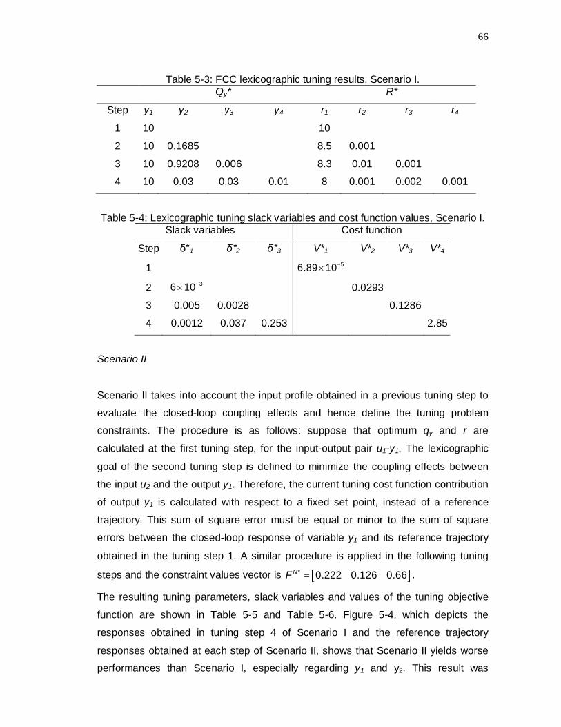
66

Table 5-3: FCC lexicographic tuning results, Scenario I. Qy* R*

Step y1 y2 y3 y4 r1 r2 r3 r4 1 10 10

2 10 0.1685 8.5 0.001

3 10 0.9208 0.006 8.3 0.01 0.001

4 10 0.03 0.03 0.01 8 0.001 0.002 0.001

Table 5-4: Lexicographic tuning slack variables and cost function values, Scenario I. Slack variables Cost function

Step δ*1 δ*2 δ*3 V*1 V*2 V*3 V*4 1 56.89 10

2 36 10 0.0293

3 0.005 0.0028 0.1286

4 0.0012 0.037 0.253 2.85

Scenario II

Scenario II takes into account the input profile obtained in a previous tuning step to

evaluate the closed-loop coupling effects and hence define the tuning problem

constraints. The procedure is as follows: suppose that optimum qy and r are

calculated at the first tuning step, for the input-output pair u1-y1. The lexicographic

goal of the second tuning step is defined to minimize the coupling effects between

the input u2 and the output y1. Therefore, the current tuning cost function contribution

of output y1 is calculated with respect to a fixed set point, instead of a reference

trajectory. This sum of square error must be equal or minor to the sum of square

errors between the closed-loop response of variable y1 and its reference trajectory

obtained in the tuning step 1. A similar procedure is applied in the following tuning

steps and the constraint values vector is * 0.222 0.126 0.66NF .

The resulting tuning parameters, slack variables and values of the tuning objective

function are shown in Table 5-5 and Table 5-6. Figure 5-4, which depicts the

responses obtained in tuning step 4 of Scenario I and the reference trajectory

responses obtained at each step of Scenario II, shows that Scenario II yields worse

performances than Scenario I, especially regarding y1 and y2. This result was

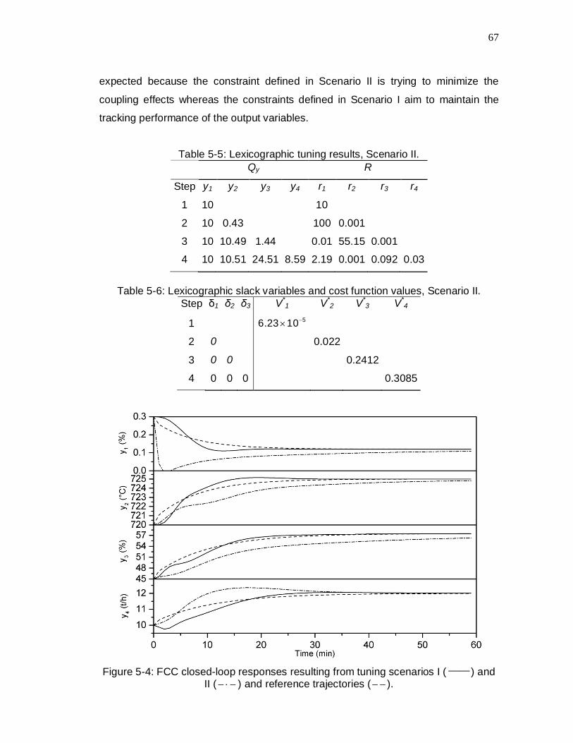
67

expected because the constraint defined in Scenario II is trying to minimize the

coupling effects whereas the constraints defined in Scenario I aim to maintain the

tracking performance of the output variables.

Table 5-5: Lexicographic tuning results, Scenario II. Qy R

Step y1 y2 y3 y4 r1 r2 r3 r4 1 10 10

2 10 0.43 100 0.001

3 10 10.49 1.44 0.01 55.15 0.001

4 10 10.51 24.51 8.59 2.19 0.001 0.092 0.03

Table 5-6: Lexicographic slack variables and cost function values, Scenario II.

Step δ1 δ2 δ3 V*1 V*

2 V*3 V*

4 1 56.23 10

2 0 0.022

3 0 0 0.2412

4 0 0 0 0.3085

Figure 5-4: FCC closed-loop responses resulting from tuning scenarios I (── ) and

II ( ) and reference trajectories ( ).

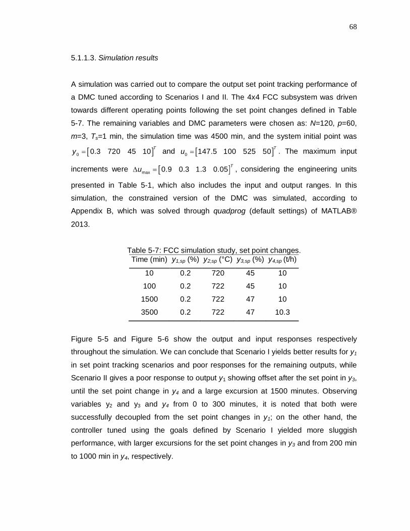
68

5.1.1.3. Simulation results

A simulation was carried out to compare the output set point tracking performance of

a DMC tuned according to Scenarios I and II. The 4x4 FCC subsystem was driven

towards different operating points following the set point changes defined in Table

5-7. The remaining variables and DMC parameters were chosen as: N=120, p=60,

m=3, Ts=1 min, the simulation time was 4500 min, and the system initial point was

0 0.3 720 45 10 Ty and 0 147.5 100 525 50 Tu . The maximum input

increments were max 0.9 0.3 1.3 0.05 Tu , considering the engineering units

presented in Table 5-1, which also includes the input and output ranges. In this

simulation, the constrained version of the DMC was simulated, according to

Appendix B, which was solved through quadprog (default settings) of MATLAB®

2013.

Table 5-7: FCC simulation study, set point changes. Time (min) y1,sp (%) y2,sp (°C) y3,sp (%) y4,sp (t/h)

10 0.2 720 45 10 100 0.2 722 45 10

1500 0.2 722 47 10

3500 0.2 722 47 10.3

Figure 5-5 and Figure 5-6 show the output and input responses respectively

throughout the simulation. We can conclude that Scenario I yields better results for y1

in set point tracking scenarios and poor responses for the remaining outputs, while

Scenario II gives a poor response to output y1 showing offset after the set point in y3,

until the set point change in y4 and a large excursion at 1500 minutes. Observing

variables y2 and y3 and y4 from 0 to 300 minutes, it is noted that both were

successfully decoupled from the set point changes in y1; on the other hand, the

controller tuned using the goals defined by Scenario I yielded more sluggish

performance, with larger excursions for the set point changes in y3 and from 200 min

to 1000 min in y4, respectively.

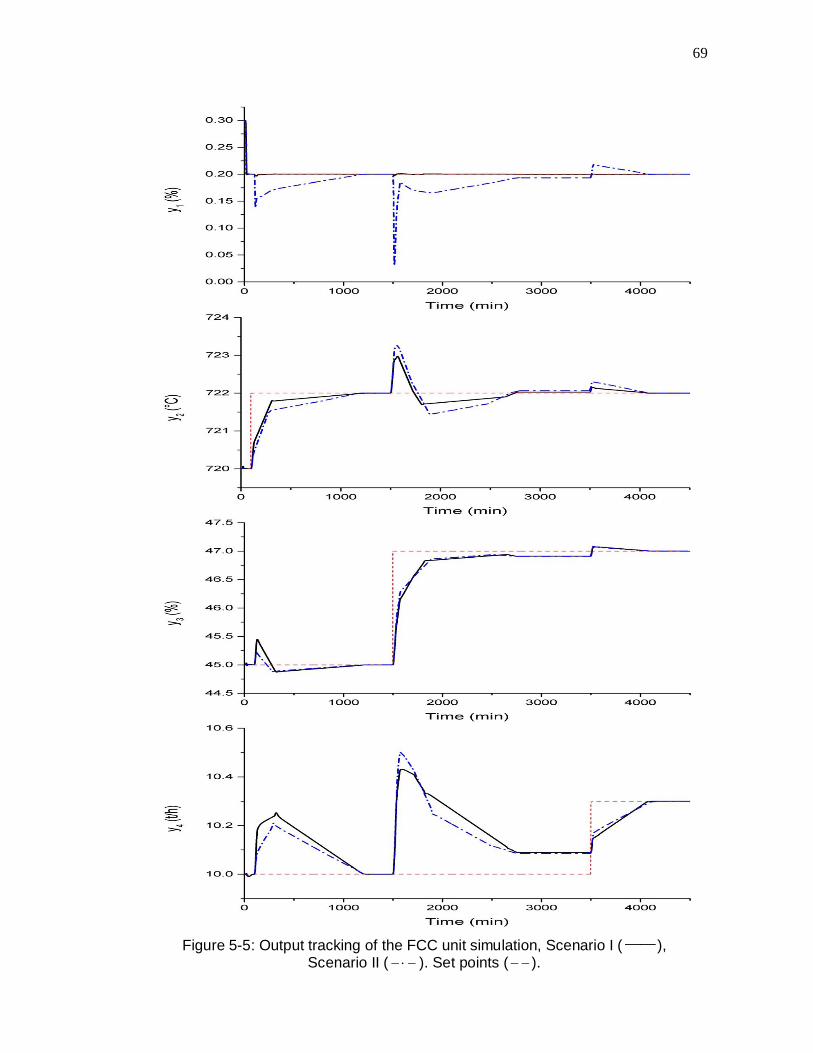
69

Figure 5-5: Output tracking of the FCC unit simulation, Scenario I (── ),

Scenario II ( ). Set points ( ).

70

Figure 5-6: Inputs of the FCC unit simulation, Scenario I (── ), Scenario II ( ).

71

It is observed in Figure 5-6 that the calculated input increments are close to their

maximum values, which is expected due to the low values of R obtained in Scenario

II. Moreover, the inputs u1, u2 and u4 saturate from 2500 to 3500 minutes, when the

DMC is trying to track the set point change of output y2. It is concluded that the goal

definitions defined in Scenarios I and II are potentially capable of defining a multi-

objective optimization tuning problem that represents the desired behavior of the

control system.

5.1.2. Heavy oil fractionator case-study

To compare the application of the tuning techniques proposed here, a MPC controller

implemented in a subsystem of the Shell Heavy Oil Fractionator (HOF) benchmark

system (Maciejowski, 2002) was tuned.

5.1.2.1. Process description

The inputs of this subsystem are the top drawn flow rate (u1), the side drawn flow rate

(u2) and the bottoms reflux heat duty (u3). The controlled outputs are the top end

point composition (y1), the side end point composition (y2) and the bottoms reflux

temperature (y3). Figure 5-7 shows a schematic representation of the process and

equation (5-7) defines the transfer functions that represent the HOF, with normalized

gains. The tuning strategies proposed here are applied to the MPC of the HOF. The

simulated scenarios involve the output tracking and the disturbance rejection.

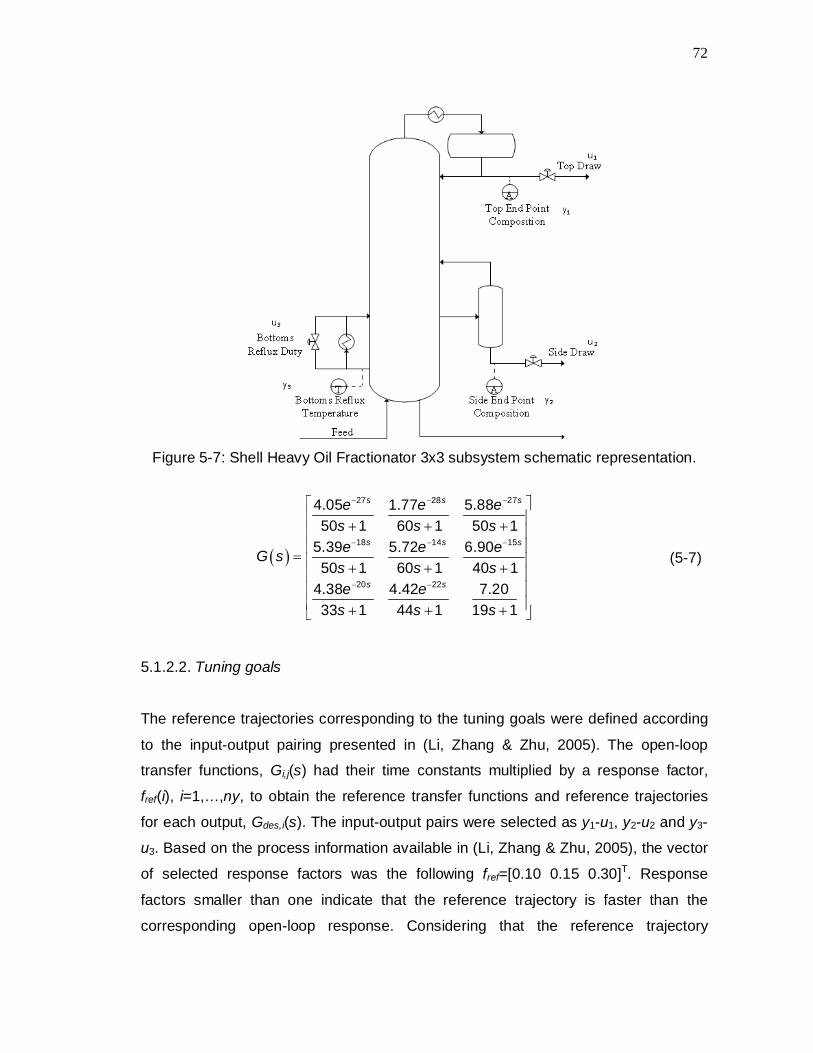
72

Figure 5-7: Shell Heavy Oil Fractionator 3x3 subsystem schematic representation.

27 28 27

18 14 15

20 22

4.05 1.77 5.8850 1 60 1 50 1

5.39 5.72 6.9050 1 60 1 40 1

4.38 4.42 7.2033 1 44 1 19 1

s s s

s s s

s s

e e es s se e eG s

s s se e

s s s

(5-7)

5.1.2.2. Tuning goals

The reference trajectories corresponding to the tuning goals were defined according

to the input-output pairing presented in (Li, Zhang & Zhu, 2005). The open-loop

transfer functions, Gi,j(s) had their time constants multiplied by a response factor,

fref(i), i=1,…,ny, to obtain the reference transfer functions and reference trajectories

for each output, Gdes,i(s). The input-output pairs were selected as y1-u1, y2-u2 and y3-

u3. Based on the process information available in (Li, Zhang & Zhu, 2005), the vector

of selected response factors was the following fref=[0.10 0.15 0.30]T. Response

factors smaller than one indicate that the reference trajectory is faster than the

corresponding open-loop response. Considering that the reference trajectory

73

corresponds to a first order plus dead time transfer function,

1

isi

desi

K eG ss

, the

resulting model parameters that define the reference trajectories for the tuning

methods proposed here are given in Table 5-8.

Table 5-8: Parameters of the reference transfer function

Output Ki τi θi y1 1 5 27 y2 1 9 14 y3 1 5.7 0

For all the outputs, the tuning horizon, θt, was assumed to be equal to 450 min, which

is large enough to encompass the responses of set point moves that drive the closed

loop system to different operating points. For the tuning procedure, the input and

output initial values are 0 0 0 0 Ty and 0 0 0 0 Tu . The output set points

are changed to 0.2 0.2 0.2 Tspy at the initial time instant, to

0.0 0.4 0.1 Tspy at time instant 150 min and to 0.1 0.3 0.0 T

spy at 300

min. Observe that this tuning scenario might be overly demanding in real

applications, because only in rare occasions more than one output set point is driven

towards new values at the same time. The control horizon is set equal to 5 and the

prediction horizon is set equal to 70. All the problems pictured here were solved

using an Intel® Core i5 320 GHz, 4 GB RAM computer. We assume that the process

model considered in the controller is ideal and that the system states are fully

measured.

5.1.2.3. MPC implemented in this case study

The controller assumes that the system is represented by the state space model in

the incremental form (5-8).

1

,x k Ax k B u ky k Cx k

(5-8)

74

where , ,nx nu nyx u y . Matrices A, B and C are the model matrices that

carry all the system information required for future output predictions.

The MPC cost function includes the weighed sum of the squared deviation of the

predicted outputs and the set point values over the prediction horizon, and the

weighted sum of squared input increments over the control horizon. The control

problem can be summarized as follows.

12 2

0 0

min ( | ) ( | )RQk y

p m

spu j j

y k j k y u k j k (5-9)

subject to (5-8) and the bounds on the inputs and input increments. The tuning

algorithms consider the unconstrained version of the MPC, disregarding the latter

bounds, so that their effects on the system inputs and input increments do not affect

the tuning results.

5.1.2.4. Tuning the MPC of the HOF system with LTT

The Lexicographic tuning problem (Problem 1) was solved for the HOF system with

the Matlab® routine fmincon, which solves a NLP. At any step w’=1,…,nu of the

tuning method, the vector of decision variables is ,1 , ' 1 ',..., , ,...,y y w wx q q r r , and the

initial guess is

10 1, ' 1 1, '5 1 1 10w wx , with the lower and upper bounds of the

decision variables equal to

2 31, ' 1 1, '5 1 10 1 10w wLB and

2 2

1, ' 1 1, '5 1 10 1 10w wUB respectively. Observe that the weight corresponding

to output y1 is kept at a fixed value (qy,1=5). Otherwise, the tuning problem would

show multiple equivalent solutions.

The weighting matrix St of the slack variables was chosen considering the expression ' 2

, 10 w it is , i=1, …, w’-1, where st,i denotes the i-th diagonal element of matrix St.

This approach guarantees that the slacks related to the more important goals will be

more heavily weighted in the tuning cost function. Observe that in the Lexicographic

approach, at any step the value of w’ corresponds to the size of the subsystem that is

considered.

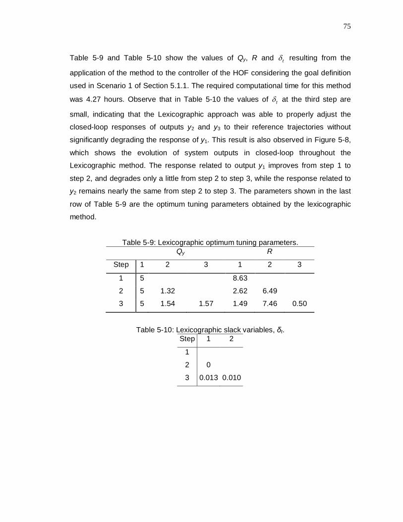
75

Table 5-9 and Table 5-10 show the values of Qy, R and t resulting from the

application of the method to the controller of the HOF considering the goal definition

used in Scenario 1 of Section 5.1.1. The required computational time for this method

was 4.27 hours. Observe that in Table 5-10 the values of t at the third step are

small, indicating that the Lexicographic approach was able to properly adjust the

closed-loop responses of outputs y2 and y3 to their reference trajectories without

significantly degrading the response of y1. This result is also observed in Figure 5-8,

which shows the evolution of system outputs in closed-loop throughout the

Lexicographic method. The response related to output y1 improves from step 1 to

step 2, and degrades only a little from step 2 to step 3, while the response related to

y2 remains nearly the same from step 2 to step 3. The parameters shown in the last

row of Table 5-9 are the optimum tuning parameters obtained by the lexicographic

method.

Table 5-9: Lexicographic optimum tuning parameters. Qy R

Step 1 2 3 1 2 3 1 5 8.63

2 5 1.32 2.62 6.49

3 5 1.54 1.57 1.49 7.46 0.50

Table 5-10: Lexicographic slack variables, δt. Step 1 2

1

2 0

3 0.013 0.010

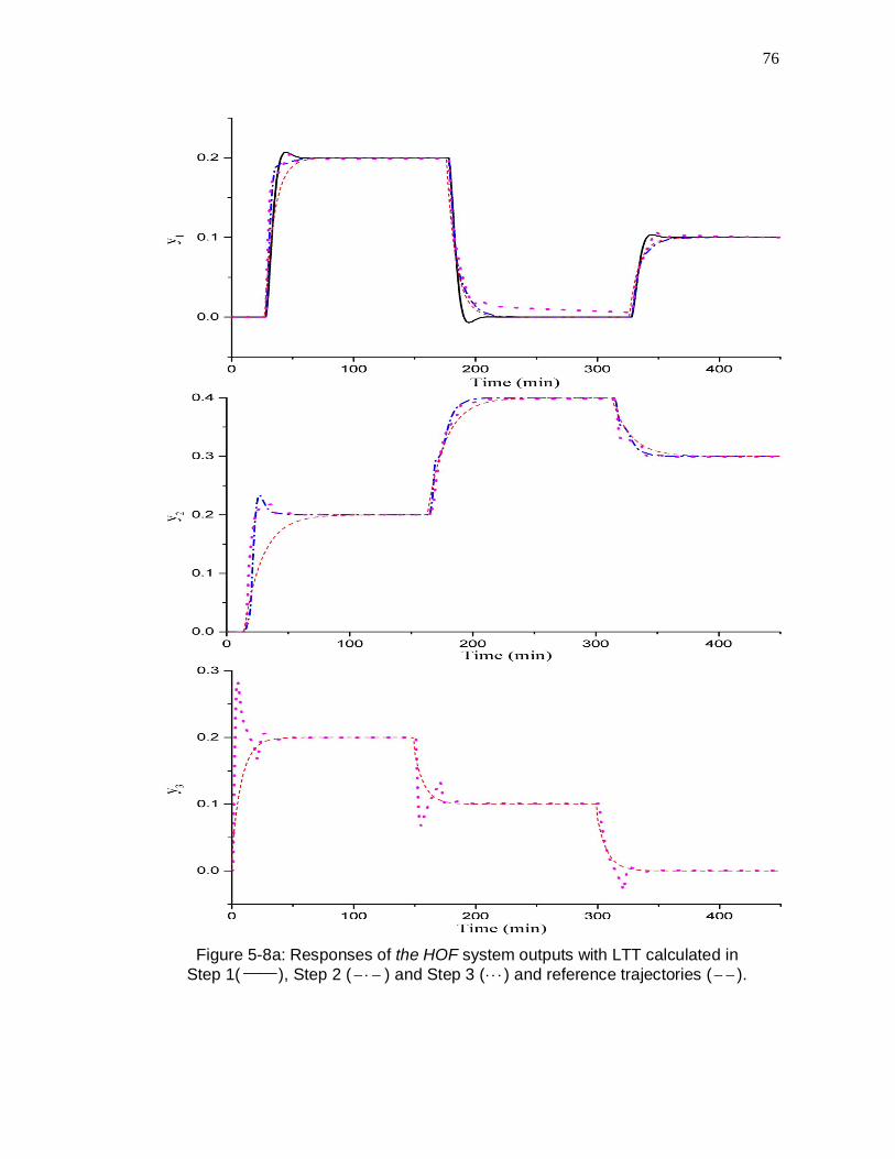
76

Figure 5-8a: Responses of the HOF system outputs with LTT calculated in

Step 1(──), Step 2 ( ) and Step 3 ( ) and reference trajectories ( ).

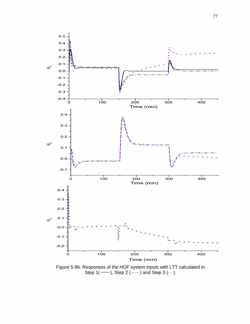
77

Figure 5-9b: Responses of the HOF system inputs with LTT calculated in

Step 1(──), Step 2 ( ) and Step 3 ( ).

78

5.1.2.5. Tuning the MPC of the HOF system with CTT

Here, it is assumed the same tuning goals as in the Lexicographic method. In the

application of the Compromise method to the Heavy Oil Fractionator, the individual

objectives of the multi-objective optimization problem are built for each controlled

output yi, according to (3-1) and, this function is minimized with respect to all the

tuning parameters to calculate the Utopia solutions, which means that each Utopia

solution defines a solution 1 1,..., , ,...,utop ny nux q q r r .

The Compromise method (Problem 2) is solved for the tuning of the MPC of the HOF

system using fmincon in MATLAB 2013®, with the following initial guess for the

tuning parameters 1

0 1,2 1,35 1 1 10x . The lower and upper bounds of the

decision variables are the same as in the Lexicographic solution of the tuning

problem. The resulting Utopia vector is 0 1.893 0.465 0.004 TF and the

optimum solution, with an execution time of 53 min, including the time required to

obtain the Utopia solution, is 5 4.96 2.91yQ diag and

3 210 2.39 10 0.982R diag .

Differently from the lexicographic approach, the number of objective defined for the

compromise tuning method is not limited to the number of inputs of the tuned system

and neither is its application to square (ny=nu) systems. It is possible to define as

many objectives as the number of system outputs, and all of them are treated

simultaneously, independently of the number of inputs. It is also observed that the

values of the parameters obtained with the compromise method are quite different

from the values of the same parameters obtained with the lexicographic method, as

seen in Table 5-11. Then, the performances of the controllers with these two sets of

tuning parameters need to be compared through closed-loop simulations.

5.1.2.6. Simulation results

Here, we analyze two different operating scenarios to compare the MPC controllers

with the parameters obtained with the tuning techniques presented earlier, addressed

in the figure captions and tables as LTT (Lexicographic technique) and CTT

(Compromise technique). The first scenario corresponds to nearly the same

79

conditions in which the MPC controlling the HOF system was tuned. Outputs are

subject to set point changes one at a time, and finally driven back to the initial

steady-state point, following the sequence of changes defined in Table 5-12. The

second simulation considers set point changes that are given in Table 5-13, as well

as unmeasured input disturbances. The different scenarios are used to validate the

tuning results. In both simulations, the constrained version of the MPC problem

defined in Section 5.1.2.3 is considered. A perfect process model and fully measured

states are assumed, and the initial operating point of the system is 0 0 0 0 Ty

and 0 0 0 0 Tu . The input lower and upper bounds and maximum input

increments are min 0.5 0.5 0.5 Tu , max 0.5 0.5 0.5 Tu ,

max 0.05 0.05 0.05 Tu .

Table 5-11: Optimum tuning parameters summary. Method Qy

* R* Computational Time LTT 5 1.54 1.57 1.49 7.46 0.50 4.27h

CTT 5 4.96 2.91 3 210 2.39 10 0.98 53 min

Figure 5-10 and Figure 5-11 show the output and input responses respectively,

corresponding to the scenario defined as Simulation I with the set-points changes

represented in Table 5-12. These figures compare the behavior of the MPC tuned

according to the methods proposed here. We observe that, although the numerical

values of the tuning parameters provided by the methods are quite different from

each other, the responses of the closed-loop system are not too different. The

responses corresponding to method LTT tend to be not the same as the CTT but

they are still close from a practical viewpoint. The same considerations can be given

to the input responses corresponding to the two methods. However the input

responses corresponding to the Lexicographic approach seems to be slightly

smoother.

Figure 5-12 and Figure 5-13 show the responses for Simulation II with the set point

changes defined in Table 5-13. The scenario is affected by an unmeasured step

disturbance of intensity 0.05 on input u1 from 40 min to 100 min. In this simulation, for

the set point changes, the responses of the two controllers seem to follow the same

80

patterns as in the previous case. However, we can observe some differences on the

responses for the disturbance rejection. The overshoots are different for the two

methods, but the largest overshoot depends on the output, and consequently, there

is not a clear superiority of any of the methods. Concerning the inputs, the two

methods seem to perform similarly, but the Lexicographic approach gives smoother

responses again. Table 5-14 shows the ISE index calculated for the output

responses and their deviation from the set points. It is observed that in both

simulations, the ISE index of the compromise strategy is lower than the ISE index of

the lexicographic strategy, and the results also support the claim that the choice of

exceedingly fast reference trajectory of output y1 lead to poor performance.

Table 5-12: Simulation I set points. Time (min) y1

sp y2sp y3

sp 1 to 80 0.2 0.2 0.2

80 to 200 0.0 0.4 0.1 200 to 300 0.1 0.3 0.0 300 to 400 0 0 0

Table 5-13: Simulation II set points. Time (min) y1

sp y2sp y3

sp 1 to 120 -0.2 0 0

120 to 200 -0.2 0 0.3

200 to 300 0 -0.2 0.3

300 to 400 0.3 0 0.2

Table 5-14: ISE index calculated for the simulation responses.

Variable y1 y2 y3 Total Technique

Simulation I LTT 3.23 3.64 0.43 7.3 CTT 3.3 3.49 1.04 7.82 Simulation II LTT 6.22 1.7 1.34 9.26 CTT 5.74 1.55 1.69 8.98

81

Figure 5-10: Simulation I. HOF outputs to set point changes ( ), LTT (── ) and

CTT ( ).

82

Figure 5-11: Simulation I. HOF inputs, LTT (──) and CTT ( ) and the upper

and lower bounds ( ).

83

Figure 5-12: Simulation II. HOF output to set point changes ( ) and unmeasured

disturbances, LTT (──) and CTT ( ).

84

Figure 5-13: Simulation II. HOF inputs, LTT (── ) and CTT ( ) and the upper

and lower bounds ( ).

85

5.1.3. Crude distillation unit case study

In this case study, the compromise technique is applied to a Crude Distillation Unit

(CDU) in closed-loop with an IHMPC control framework. First, we provide a brief

description of CDU, along with specific information about the particular unit from the

Capuava Refinery, Brazil. Then, we define the goals and show the optimum tuning

parameters. Finally, we compare tuning results to another multi-objective tuning

technique from the literature and to the pre-existing parameters in a simulation

including set point changes and disturbance rejection scenarios.

The CDUs are certainly one of the most important, complex and energy-intensive

processes in oil refineries (Liau, Yang & Tsai, 2004; Luo, Wang & Yuan, 2013). It is

also one of the most common separation process units in the chemical industry (Seo,

Oh, & Lee, 2000). Moreover, all the crude oil must initially go through a CDU before

being further processed in subsequent refining units. Even though chemical reactions

do not take place along the distillation process, the amount of mass and energy

involved, the number of equipment, the environmental and operational constraints,

and the conflicting financial goals are sufficient to make the CDU system a

challenging control problem.

The crude oil stream contains an array of different kinds of hydrocarbons along with

other organic and inorganic compounds (Seo, Oh & Lee, 2000). It is not practical to

precisely determine the feedstock composition and to set the operating conditions of

the distillation unit in order to deal with that specific composition, therefore, a reliable

automated control framework is imperative to enforce safe and stable operation, and

to achieve high product quality while meeting production rate goals (Mizoguchi,

Marlin & Hrymak, 1995).

Another complicating issue arises from the fact that it is not straightforward to assess

product quality. Diesel, kerosene, gas oil and naphtha are the main products of a

CDU and there is few expensive and hard to maintain hardware available to measure

density, viscosity, flash points (Chatterjee & Saraf, 2004), gravity, sulfur content and

composition of such product streams (Liau, Yang & Tsai, 2004). In practice, it is

common to correlate the temperature and flow rates measures of the outlet streams

with physical properties resulting from offline laboratorial assessments of ASTM

(America Society for Testing Materials) standardized tests, such as the D86 curves of

distillated oil products. For example, Chatterjee & Saraf (2004) established a method

86

to infer product properties such as densities, flash points, pour points and recoveries

for gas oils, and the freezing point of the kerosene from the crude oil true boiling

point and other routinely measured variables during the CDU operation. Trial

inference applications showed satisfactory results; however, the authors recommend

extensive tests prior to real applications.

CDUs are usually comprised of a pre-flash column, an atmospheric distillation

column and a vacuum distillation column, along with side stripping sections, heat

exchangers, and pump around reflux streams. The heat recovery problem, i.e.

determine an optimum arrangement of pump around streams to minimize the heat

required to raise the crude oil temperature up to its required value at the inlet of the

pre-flash or atmospheric distillation column, is just one of the complications that arise

in CDU optimization. The oil industry is also concerned with maximizing profit and

enforcing product standards.

The control and optimization of the CDU unit has been extensively studied in the

literature. There are different approaches to address CDU optimization. Liau, Yang &

Tsai (2004) developed a neural network model to correlate quality parameters and

measurable process variables to optimize the CDU operation. The neural network

training data was collected over a period of six months and the results showed that

the method can provide useful insight for inexperienced operators. Luo, Wang &

Yuan (2013) used a shortcut method (SCFrac) in ASPEN Plus® to simulate

distillation columns using real input parameters such as column pressure, estimated

product flow, number of theoretical stages, steam flow and product specifications. A

multi-objective optimization was assembled to find an optimum operating point

considering energy cost and profitability goals. The authors solved the problem using

PSO. Seo, Oh & Lee (2000) developed an algorithm to determinate the optimum feed

tray, in terms of maximizing heat recovery along the process, and to determine

optimum operational conditions to yield the minimum annual operational cost. The

optimization problem was posed as a MINLP, solved using GAMS®. Mizoguchi,

Marlin & Hrymak (1995) proposed a first principle description of a CDU from Petro-

Canada. Process optimization was done in terms of the advanced control framework,

in which an upper RTO layer provides optimum controlled and manipulated variables

targets for a lower QDMC control algorithm. In the simulated studies, the QDMC uses

a linearized process model, whereas the real plant is represented through to the first-

principle model. The results showed that control strategies should be carefully

87

studied since some variables might drive the process to better operational points.

Moreover, the authors concluded that it is imperative to ensure that the control

system can take into account the process disturbances.

5.1.3.1. Process description

The system studied here is a process unit of the RECAP refinery of Petrobras,

located in São Paulo, Brazil that processes about 50,000 bbl/day of light crude oil.

Figure 5-14 shows a schematic representation of the unit, including the relevant

process equipment, streams and regulatory control loops. The crude preheating

system consists of one preheating train with two desalters operating in series. The

pre-flash column N-507 separates light naphtha and light diesel from the crude. Its

bottom product is preheated in two parallel trains of heat exchangers and is partially

vaporized in the furnace L-506, before being fed to the atmospheric fractionator N-

506, which produces: heavy naphtha, kerosene, heavy diesel and the atmospheric

residue. Kerosene and heavy diesel are blended to produce the commercial diesel

product. The bottom product is sent directly to a Residue Catalytic Cracking Unit.

5.1.3.2. Control strategy, variables and economic goals

The economic objectives of the CDU, in order of priority, are: (i) maximize the diesel

production by minimizing the flow rates of heavy naphtha and atmospheric residue,

and enforce that its specifications are satisfied (minimum bound on the flash point

and a maximum bound on the ASTM D-86 distillation curve 95%); (ii) supply the

required amount of light naphtha that feeds the solvent unit; (iii) minimize the flow

rate of stripping steam injected into the system; (iv) minimize the consumption of fuel

oil at the preheating furnace.

Based on the objectives defined above that are related to the profit optimization, the

unit operating goals are listed as follows: 1) The crude oil flow rate (u1) should be

maximized in all the scenarios. 2) The flow rate of the stripping steam to the pre-flash

column (u3) should be driven to its target that is calculated by the RTO layer. 3) The

light naphtha outlet stream flow rate (y9) and the ASTM D-86 end point (y7) are

important controlled variables to ensure the appropriate quantity and quality of the

light naphtha sent to the solvent production unit. 4) The pre-flash overhead

88

temperature set-point (u2) is a manipulated variable with direct influence on the light

naphtha quality, but it is constrained by the top reflux flow rate (y8). 5) Two properties

of the diesel must be enforced as constraints, its flash point (y6) and its ASTM D86

95% (y5). The former is important in the minimization of the fractionator top

temperature (u4). This minimization is constrained by the minimum bound on the

heavy naphtha flow rate (y2) and by the maximum bound on the reflux flow rate (y3).

The ASTM D86 95% constraint tends to become active when the outlet temperature

of the crude furnace (u8) is maximized, which is also constrained by the maximum

bound on the furnace heat duty (y10). 6) The pumparound flow rate (u6) should be

maximized in order to save fuel in the furnace. It is constrained by the ratio between

kerosene and heavy diesel that can be represented by the kerosene withdraw

temperature (y4). 7) The diesel pumpdown reflux flow rate (u5) should be manipulated

to improve the fractionation between the heavy diesel and the atmospheric residue.

The controlled and manipulated variables are illustrated in Figure 5-14, and are

described in Table 5-15 and Table 5-16, respectively, along with their operational

bounds and usual values. The output set points, or control zones are enforced

directly by the MPC, while the input targets are calculated at the RTO layer. The

reader can find the system transfer functions, obtained from operational data of the

CDU industrial system, in Appendix A.

Figure 5-14: Schematic Representation of Crude Distillation Unit.

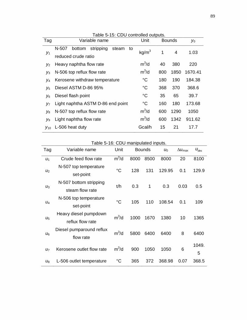
89

Table 5-15: CDU controlled outputs. Tag Variable name Unit Bounds y0

y1 N-507 bottom stripping steam to

reduced crude ratio kg/m3 1 4 1.03

y2 Heavy naphtha flow rate m3/d 40 380 220 y3 N-506 top reflux flow rate m3/d 800 1850 1670.41 y4 Kerosene withdraw temperature °C 180 190 184.38 y5 Diesel ASTM D-86 95% °C 368 370 368.6 y6 Diesel flash point °C 35 65 39.7 y7 Light naphtha ASTM D-86 end point °C 160 180 173.68 y8 N-507 top reflux flow rate m3/d 600 1290 1050 y9 Light naphtha flow rate m3/d 600 1342 911.62 y10 L-506 heat duty Gcal/h 15 21 17.7

Table 5-16: CDU manipulated inputs. Tag Variable name Unit Bounds u0 ∆umax desu

u1 Crude feed flow rate m3/d 8000 8500 8000 20 8100

u2 N-507 top temperature

set-point °C 128 131 129.95 0.1 129.9

u3 N-507 bottom stripping

steam flow rate t/h 0.3 1 0.3 0.03 0.5

u4 N-506 top temperature

set-point °C 105 110 108.54 0.1 109

u5 Heavy diesel pumpdown

reflux flow rate m3/d 1000 1670 1380 10 1365

u6 Diesel pumparound reflux

flow rate m3/d 5800 6400 6400 8 6400

u7 Kerosene outlet flow rate m3/d 900 1050 1050 6 1049.

5

u8 L-506 outlet temperature °C 365 372 368.98 0.07 368.5

90

5.1.3.3. Definition of the tuning goals

In the previous section, it was listed all the important inputs that should be driven to

their targets and the outputs that should be kept inside their control zones. The MPC

tuning analysis presented in this work will consider two different scenarios. The first

one will focus only at the output tracking performance of the controller. This means

that the weighting matrices Qy, and R are selected solely based on the performance

of the output responses. The second scenario will consider output and input tracking

simultaneously, and tuning will focus on Qy, Qu, and R.

The compromise method proposed here is compared with a MPC tuning technique

from the literature that is also based on multi-objective optimization. Hereafter this

technique is addressed as the Normal Boundary Intersection (NBI) approach. It is

based on a posteriori choice of the optimum solution from a set of non-dominated

solutions. The set of solutions is obtained through a grid search over an evenly

spaced parameterized unitary segment is for each objective. The searching points

lie on the (quasi-) normal direction e to a plane defined by the individual

optimum solutions, indicated by s . The following optimization problem is solved:

Problem 3

,minx X

(5-10)

Subject to

,11nys F x F (5-11)

1

0, 1i ii

s s . The i-th column of the pay-off matrix is defined as iF x F

The reader is referred to (Das & Dennis, 1998; Vallerio, van Impe & Logist, 2014)

and the references therein for more information. The NBI method was implemented

using an increment of 0.5 to define the vector s . The decision regarding the best

Pareto solution was done following the weighted sum method (Pohekar &

Ramachandran, 2004), in which a performance index named WSM is calculated

according to (5-12). The non-dominated solution that yields the largest index value is

selected as the best solution.

91

1

, 1 ,,w

ij jj

WSM a f i M (5-12)

where w is the number of objectives, M is the number of non-dominated solutions, fj

is the j-th objective weight and aij is the value of the cost function of the j-th objective

calculated using the i-th Pareto solution.

The objective weights of the output tuning approach are the inverse of the response

factors, i.e. 1

outputres

ff

, and the input tuning approach weighting vector was chosen

arbitrarily as 1 2 3 4 5 6 7 8inputf .

The two tuning approaches considered here consider the following lower and upper

bounds for the tuning parameters, which correspond to Qy, Qu, and R:

3 2

1 1 11 1 10 1 10ny nu nuLB , 2

1 1 11 20 1 0.1 1 10ny nu nuUB ; and the

tuning horizon is 300t min.

In all the cases considered here, the transfer function gains, inputs and outputs are

normalized considering the input and output operating ranges. The control horizon is

chosen as m=5. These parameters were selected following the literature guidelines

and also based on the analysis of the simulation results. The MPC control problem

was solved analytically, disregarding the constraints. The CTT multi-objective

optimization problem (Problem 2) and the NBI problems (Problem 3) ware solved

using fmincon (default settings), MATLAB® 2013, on an Intel ® Core i5, 3.20Ghz,

4Gb RAM computer. The MPC with input targets and output zone control and its

analytical solution are introduced in Appendix B.

5.1.3.4. Tuning the MPC for the output set point tracking scenario

The selection of the input-output pairs for the definition of the reference trajectories is

performed based on the input-output relationship matrix represented in Table 5-17

and the RGA approach (Bristol, 1966). Since the closed loop transfer functions relate

the outputs with their set points, all the gains are unitary, and the time constants are

obtained by multiplying the time constants of the approximate transfer functions by

the response factors defined below:

92

0.25 0.30 0.45 0.50 0.55 0.70 0.85 0.90 1.0 1.0resf

Table 5-18 summarizes the transfer functions that define the reference trajectory for

each output. In the tuning scenario corresponding to the output tracking, matrix uQ is

not included as a decision variable of the tuning problem. Therefore, the objective

function of the MPC considered here does not include the term corresponding to the

input target. Also, spy is considered as a pre-defined parameter, instead of a decision

variable of the MPC problem, because the main focus of this tuning step is to obtain

a set of parameters such that the MPC will be capable of adequately driving the

outputs back to their zones when a disturbance affects the CDU system. To compute

the values of function (3-1) that characterizes the performance of the controller, the

system starts from a steady state that corresponds to 50% of the nominal output

values and corresponding input values. The outputs are all inside of their control

zones and the output set points are moved to a value equal to 75% of their nominal

value at time instant 1 min. At time instant 100 min, they are moved to values equal

to 50% of the nominal values and finally, at time 200 min, the set points are fixed at

25 % of the nominal values.

The tuning parameters resulting from the application of the proposed Compromise

method to this first scenario are the following:

1 2.07 1 1 1 2.93 8.3 20 10.2 1.34yQ diag ,

0.65 0.011 0.01 0.01 0.01 0.01 0.01 0.01R diag

and the tuning parameters obtained with the application of the NBI method are the

following:

1 20 1 1 1 1 1 20 1.54 4.41yQ diag ,

0.01 3.49 0.11 0.01 0.012 0.01 0.015 0.235R diag . The parameters

originally implemented in the MPC of the real CDU system are

5 2 1 3 10 5 5 1 10 20yQ diag , 1 1 1 1 1 1 1 1uQ diag ,

0.1 6 2.93 5 0.15 4 1 20R diag .

The performance of the controller with this tuning set, addressed here as ‘Existing’, is

also compared to the other tuning sets obtained here.

93

Table 5-17: CDU input-output relationship matrix. u1 u2 u3 u4 u5 u6 u7 u8

y1

x y2

x

x y3

x

x

x x x

y4

x

x x x

y5

x x

x x

y6

x

x x y7

x x y8 x x x y9 x x x y10 x x x x

Table 5-18: Reference trajectories transfer function time constants. Output Input Time constant

y1 u3 1.1080 y2 u4 12.6710 y3 u6 1.0684 y4 u7 10.6011 y5 u5 8.3741 y6 u4 2.7598 y7 u2 8.1778 y8 u3 7.3582 y9 u1 32.0422 y10 u8 3.8556

It is observed that there are significant differences between some of the tuning

parameters produced by the two methods. We also observe that the existing tuning

parameters of the CDU controller are quite different from the parameters obtained

here.

The performances of these three sets of parameters are compared in a simulated

scenario in which five outputs are driven to different set points, following the pattern

proposed in the tuning section, while the remaining outputs are assumed to remain

within their control zones. Figure 5-15 shows the closed-loop responses of the

94

selected outputs. It is also shown the responses of the controller with the parameters

corresponding to the utopia solution.

It is observed from Figure 5-15 that the responses of the MPC with the tuning

parameters defined through the compromise method are closer to the Utopia

responses than the MPC tuned through the NBI method. We also observe that the

existing tuning parameters are quite conservative and lead to more sluggish

responses than the tuning parameters obtained here. The controllers resulting from

the two tuning techniques analyzed here successfully tracked all the output set

points, but the existing controller failed to track the set point moves of 3y within the

simulation horizon considered here.

95

Figure 5-15a: Output tracking tuning analysis, CTT (── ), NBI ( ),

existing controller ( ), Utopia ( )

96

Figure 5-15b: Output tracking tuning analysis, CTT (── ), NBI ( ),

existing controller ( ), Utopia ( )

97

5.1.3.5. Tuning for the input target tracking scenario

As seen in Table 5-18, each input of the CDU system is related to several outputs

through non-zero transfer functions. This multivariable character may result in a

conflict between the input targets and the output zones. This means that some of the

outputs may tend to be driven to outside their zones when the MPC forces the inputs

toward their targets. The tuning parameters of the MPC should be selected such that

this conflict is minimized in the practical case. This means that if the input targets are

unreachable, the priority should be to keep the outputs inside the control zones and

allow for offset in the inputs. The following paragraphs present some specific

scenarios where an input is driven to a target while one or more associated outputs

tend to be driven to the border of their control zones, becoming active constraints.

The reference trajectories for the inputs are defined as linear functions with angular

coefficient corresponding to maxu . The output constraints over the input optimization

are included for the outputs strongly correlated with the input. Observe that, here the

definition of the input tuning objective is more complex, and it is heavily dependent

on a practical knowledge of the process system and its operating peculiarities. It is

assumed that the output initial value lies in the middle of its operating range and at

time instant 1 min, their set points are changed to 75% of their nominal values. The

inputs initial conditions and targets, in the units shown in Table 5-15 and Table 5-16

are 0 8000 128 1 110 1271.5 6400 1050 372 Tu

and 8125 128.75 0.825 108.75 1439.1 6250 1012.5 370.25 Tdesu .

Each of the cases described below considers one input with its target. The outputs

more heavily connected to this input and that can reach a constraint are also

considered one at a time, even though, in practice, the input may be constrained by

more than one output simultaneously. In the definition of the tuning goal related with

each case, it is assumed that the output should be driven to a set point, while the

input should follow a trajectory towards its target.

Objective I – Flow rate of crude to the CDU

The target to the flow rate of crude oil (u1) is defined by the RTO layer that tries to

force the maximization of the flow rate of diesel that is produced by the CDU. The

outputs that may constrain the input optimization are the light naphtha flow rate (y9)

98

and the furnace heat duty (y10). Only the latter is considered in the definition of this

tuning objective.

Objective II – Flow rate of diesel pumparound

The diesel pumparound flow rate (u6) is set by the RTO to maximize the heat that is

recovered in the crude oil preheating trains and to save fuel oil/gas in the heating

furnace. This input is mainly constrained by the top reflux flow rate of the main

fractionator (y3).

Objective III – Flow rate of stripping steam

The RTO layer computes an optimum target to the flow rate of the stripping to the

bottom of the pre-flash column (u3) in order to maximize the flow rate of light naphtha

that is produced by the CDU. The related output constraints are the pre-flash reflux

flow rate (y8) and the ratio between the flow rate of the stripping steam and the flow

rate of reduced crude (y1). The former is chosen in the definition of this objective.

Objective IV – Temperature at the top of the pre-flash column

The set point to the controller of the temperature at the top of the pre-flash column

(u2) is set by the RTO to maximize the production of light naphtha. The constraints

associated with this target are the bounds of the light naphtha flow rate (y9) and the

maximum D-86 end point of the light naphtha (y7). Here, the objective is formulated in

terms of y9 only.

Objective V – Temperature at the top of the atmospheric column

The RTO sets a target to the set point of the temperature controller at the top of the

fractionator (u4) in order to maximize the production of heavy naphtha. The

constraints associated with this input are the bounds on the heavy naphtha flow rate

(y2) and the bounds on the diesel flash point (y6). The objective pair is selected in

terms of y2

Objective VI – Flow rate of heavy diesel pumpdown reflux

The target to the flow rate of the heavy diesel pumpdown reflux in the fractionator (u5)

is set by the RTO to maximize the production of diesel. This target may be

constrained by the diesel ASTM D-86 95% (y5).

99

Objective VII – Kerosene outlet flow rate

The kerosene outlet flow rate (u7) is also set by the RTO when the diesel production

is maximized. This target may be constrained by the temperature of the tray where

the kerosene is drawn from the atmospheric column (y4).

Objective VIII – Furnace temperature

The temperature at the outlet of the crude heating furnace (u8) is also set by the

RTO. This target may be constrained by the diesel ASTM D-86 95% specification

(y5).

Two different approaches are proposed: in Scenario II-A, the optimum values of yQ

and R obtained in Section 5.1.3.4 are inherited and used as fixed parameters

instead of decision variables. In Scenario II-B, the elements of matrices yQ , uQ and

R are considered as decision variables of the tuning problem.

The input tracking analysis compares the closed-loop responses with the controller

tuned through the Compromise method using approaches II-A and II-B to the

controller with the existing parameters. The following pairs were chosen to illustrate

the closed-loop performance of the MPC for the input tracking scenario: y3-u6, y8-u3,

and y10-u1, which represent the objectives II, III, and I, respectively. The remaining

outputs are assumed to be kept within their control zones and other inputs do not

have active targets, where the input references are also included. Table 5-19 shows

the optimum tuning parameters From Figure 5-16, we observe that the output

responses of the controllers tuned with the two scenarios are fast and not too

different from each other, but the CTT II-A tends to produce an oscillatory behavior,

which is not desirable in practice. The performance of the MPC based on the CTT II-

B method is slightly more sluggish but not oscillatory. Regarding the input reference

trajectories, none of the proposed tuning approaches yielded an outstanding tracking.

This shows that the compromise approaches prioritize the control of the system

outputs while the optimizing input targets will be tracked only after the outputs have

been driven to their set points.

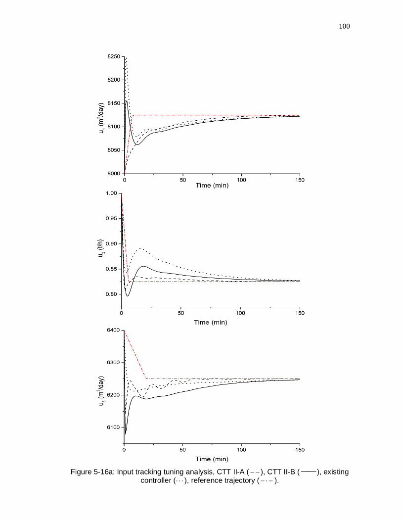
100

Figure 5-16a: Input tracking tuning analysis, CTT II-A ( ), CTT II-B (── ), existing

controller ( ), reference trajectory ( ).

101

Figure 5-16b: Input tracking tuning analysis, CTT II-A ( ), CTT II-B (── ), existing

controller ( ), reference trajectory ( ).

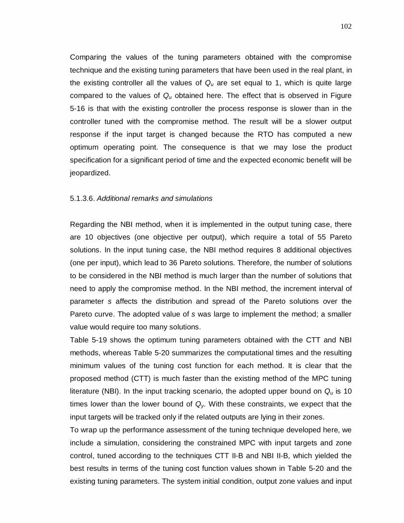
102

Comparing the values of the tuning parameters obtained with the compromise

technique and the existing tuning parameters that have been used in the real plant, in

the existing controller all the values of Qu are set equal to 1, which is quite large

compared to the values of Qu obtained here. The effect that is observed in Figure

5-16 is that with the existing controller the process response is slower than in the

controller tuned with the compromise method. The result will be a slower output

response if the input target is changed because the RTO has computed a new

optimum operating point. The consequence is that we may lose the product

specification for a significant period of time and the expected economic benefit will be

jeopardized.

5.1.3.6. Additional remarks and simulations

Regarding the NBI method, when it is implemented in the output tuning case, there

are 10 objectives (one objective per output), which require a total of 55 Pareto

solutions. In the input tuning case, the NBI method requires 8 additional objectives

(one per input), which lead to 36 Pareto solutions. Therefore, the number of solutions

to be considered in the NBI method is much larger than the number of solutions that

need to apply the compromise method. In the NBI method, the increment interval of

parameter s affects the distribution and spread of the Pareto solutions over the

Pareto curve. The adopted value of s was large to implement the method; a smaller

value would require too many solutions.

Table 5-19 shows the optimum tuning parameters obtained with the CTT and NBI

methods, whereas Table 5-20 summarizes the computational times and the resulting

minimum values of the tuning cost function for each method. It is clear that the

proposed method (CTT) is much faster than the existing method of the MPC tuning

literature (NBI). In the input tracking scenario, the adopted upper bound on Qu is 10

times lower than the lower bound of Qy. With these constraints, we expect that the

input targets will be tracked only if the related outputs are lying in their zones.

To wrap up the performance assessment of the tuning technique developed here, we

include a simulation, considering the constrained MPC with input targets and zone

control, tuned according to the techniques CTT II-B and NBI II-B, which yielded the

best results in terms of the tuning cost function values shown in Table 5-20 and the

existing tuning parameters. The system initial condition, output zone values and input

103

targets are given Table 5-15 and Table 5-16 and correspond to a typical operating

condition. It is assumed that the system starts from a condition where the input target

and all the computed output set points lie in their operating ranges and,

consequently, the inputs are not constrained by the output zones. In this case, the

MPC can drive the system inputs to their targets without offset. This scenario can be

observed in Figure 5-17 and Figure 5-18, from 0 min until 1000 min. In this case, all

the inputs reach their targets and the outputs stabilize in the control zones.

Table 5-19: Tuning results for Scenario II-A and II-B. CTT NBI

II-A II-B II-A II-B Qu Qy Qu R Qu Qy Qu R 0.1 1 0.1 0.035 0.001 1 0.099 0.082 0.1 2.359 0.1 0.03 0.1 2.067 0.001 0.01 0.1 1 0.1 0.142 0.001 1.746 0.001 0.01 0.1 1 0.1 0.044 0.1 1.6 0.1 1.497

0.001 1 0.001 0.01 0.1 1.006 0.1 0.202 0.1 1 0.1 0.01 0.1 3.857 0.001 0.075 0.1 1.924 0.1 9.435 0.1 1 0.018 0.028

0.061 3.012 0.018 5.048 0.1 1 0.076 2.499

1

1

1

4.616

Table 5-20: Tuning strategies comparison. Method Elapsed time (h) Total cost fuction value

Scenario I CTT 2.54 9.34 NBI 68.37 12.52 Utopia 1.03

Scenario II-A CTT 0.69 237 NBI 24.5 385.7 Utopia 1.4

Scenario II-B CTT 7.34 180.5 NBI 34.5 241.76 Utopia 2.91

104

At time instant 1000 min, the target of input u5 is changed from 3,5 1365 /desu m d to

3,5 1250 /desu m d , which is unreachable because it corresponds to a steady state

where y5 would lie above its maximum bound. From Figure 5-17, we observe that the

output responses of the closed loop system with MPC tuned with the proposed

method are similar to the responses of MPC with the existing parameters, however

the responses obtained by the set of parameters obtained by the NBI were strange,

with large excursions. The three controllers try to drive u5 to its new target, which

cannot be reached because y5 reaches its maximum bound. We observe that all the

controllers with the different sets of tuning parameters behave adequately in the

sense that the maximum bound on y5 is not surpassed but inputs u4, u5, u7 and u8

that have non-zero transfer functions relating them to y5, tend to show offsets with

respect to their targets. Figure 5-18 shows that the three controllers stabilize the

system at a new steady state where the offsets in the inputs are distributed differently

by each controller. We also observe that the responses of inputs u6 and u7 show

some large excursions for the controller tuned with the NBI method.

At time instant 2000 min, the target of input u1 is changed from 3,1 8100 /desu m d to

3,1 8470 /desu m d . With this new target, the controller tends to be constrained by the

upper bound on output y10. Again the three controllers try to drive the CDU system to

an optimum point that is unreachable, and the offset is distributed between inputs u1,

u2, u3 and u8, which are the inputs that are related to y10. The MPC tuned with the

method proposed here behaves similarly to the existing MPC tuned with ad-hoc

procedures based on trial and error. However, the former shows large excursions

upon the second input target change for u6 and u8, which as attributed to the low

value of the upper bounds on Qu. Again, the MPC tuned with the NBI method shows

unjustified large excursions of inputs u2 and u3.

105

Figure 5-17: Outputs of the CDU in closed loop simulation with MPC tuned with

CTT II-B (──), NBI II-B ( ), existing controller ( ) and bounds ( ).

106

Figure 5-18a: Inputs of the CDU in closed loop simulation with MPC tuned with

CTT II-B (── ), NBI II-B ( ), existing controller ( ) and targets ( ).

107

Figure 5-18b: Inputs of the CDU in closed loop simulation with MPC tuned with

CTT II-B (── ), NBI II-B ( ), existing controller ( ) and targets ( ).

108

Figure 5-18c: Inputs of the CDU in closed loop simulation with MPC tuned with

CTT II-B (── ), NBI II-B ( ), existing controller ( ) and targets ( ).

109

5.2. Tackling the model uncertainty

The case study presented here is an application of the extended robust tuning

techniques developed here to an infinite horizon MPC in closed-loop with a C3/C4

splitter system. The formulation of the IHMPC and RIHMPC used in this case study

are presented in Appendix B.

5.2.1. Nominal IHMPC performance under plant-model mismatch

Porfírio, Neto & Odloak, (2003) identified 6 different transfer function models from the

operational data of a C3/C4 splitter, as seen in Appendix A. Figure 5-19 shows the

system schematic representation and Table 5-21 lists the tags, names, ranges and

engineering units of the inputs and outputs.

Figure 5-19: Schematic view of the C3/C4 splitter system, (Porfírio, Neto & Odloak,

2003).

Table 5-21: List of variables of the C3/C4 splitter system. Tag Variable Range Unit

y1 C3 % in the butane stream 0.80 - 1.20 % y2 Top temperature 43 – 54 °C u1 Reflux flowrate 2000 - 4100 m3/d u2 Hot fluid flowrate 1200 - 2200 m3/d

110

Table 5-22: Set point changes of the C3/C4 Simulation I. Time instant (min) y1,sp (%) y2,sp (°C)

0 0.99 48 100 0.85 49 300 0.9 51 500 0.95 50

The simulation shown in Figure 5-20, addressed as Simulation I, illustrates the plant-

model mismatch effects. The initial state of inputs and outputs is 0 1.1 50 Ty and

0 2200 1300 Tu . The upper and lower bounds on the inputs and outputs were

taken from Table 5-21, and max 50 25 Tu . The simulation ran for 550 minutes

and the set point changes are listed in Table 5-22, the system was in closed-loop

with an IHMPC, with the following tuning parameters: Ts=1 min, m=5,

5 510 10yS diag ,

5 510 10iS diag , 10 0.5yQ diag and

0.71 0.06R diag . Matrices Qy and R were obtained using the nominal

lexicographic approach, whose procedure was omitted for brevity. Considering that

the IHMPC is based on the real plant model that is assumed to be model 6. A

Kalman filter was used to estimate the system states, based on the difference

between current and predicted output values; the process and measurement noise

covariance matrices were set equal to unit matrices of appropriate dimensions. The

‘real’ plant changes from the nominal model (model 6) to model 1 at 100 minutes.

Observe that the nominally tuned IHMPC is unable to track the set point changes and

yields oscillatory responses.

111

Figure 5-20: C3/C4 splitter model-plant mismatch Simulation I, LTT IHMPC

responses ( ) and set points or bounds ( ).

112

5.2.2. Robust LTT tuning

The robust Lexicographic approach takes into account all the 6 models

simultaneously, as described in Section 3.3, to find a set of tuning parameters that

yields a robust operation in plant-model mismatch scenarios.

The tuning horizon was chosen as 60t , and the pair y1-u2 was deemed more

important than y2-u1. desG s was chosen based on first order approximations of the

open-loop step responses of transfer functions 2,1G s and 1,2G s of the nominal

model. The time constants of ,1,1desG s and ,2,2desG s were set to 10% and to 30%

of the first-order approximations as shown in (5-13). The system initial conditions and

output set points were: 0 0.277 1.630 Ty , 0 0.6 0.7 Tu , 0.272 1.581 Tspy ,

considering the normalized values defined in (5-3) and (5-4); the robust

Lexicographic problem, defined by equations(3-9) - (3-13), was solved using fmincon

(tolfun = 1010 , tolx = 1010 , maxfunevals = 34 10 , tolcons = 610 , maxiter = 24 10 )

and the IHMPC control problem was solved analytically in MATLAB® 2013. The

decision variable vector was ,1 , ' 1 'y y w wx q q r r ; its initial guess, lower,

and upper bounds for the tuning parameters were: 2' 10 '0 101 w wx 1 1 ,

' 1 '0.10 5w wLB 1 1 and 2 3

' 1 '10 010 1w wUB 1 1 ; the initial values,

lower and upper bounds of slack variables were vectors of ones, zeros and 610 with

appropriate dimensions, respectively; 8 8 6 8 6 310 10 10 10 10 10rS diag

and 66 10pS I . The optimum tuning parameters obtained by the robust

Lexicographic technique were Qy=diag([10 3.87]) and R=diag([129.91 100]). The total

time elapsed was 247 minutes on an Intel® Core™ i5 3.20 GHz, 4Gb RAM

computer. Figure 5-21 and Figure 5-22 show the set point tracking output responses

for all six models, and its reference trajectory.

1 02 1

107.8 1

dessG s

s

(5-13)

113

Figure 5-22 shows that the optimum solution yields poor performances for models 4

and 3, i.e. excessive sluggishness, and large overshoot, respectively. The right hand

graph of Figure 5-22 shows that the 2y set point tracking is only achieved for model

6, within the tuning horizon. However, all the trajectories are stable. The sluggish

responses observed in the left hand graph, for variable y1 are necessary in order to

stabilize all the responses obtained in the model mismatch scenario, taking into

account all the models in Ω.

Penalizing the robustness slack variable of model 2 improved the reference trajectory

tracking performance in the second tuning step. On the other hand, model 4 did not

improve.

114

Figure 5-21: C3/C4 splitter RLTT, output responses of the first step.

Figure 5-22: C3/C4 splitter RLTT, output responses of the second step.

115

5.2.3. Robust CTT application

In this section, we use the robust compromise approach to tune an IHMPC in closed-

loop with the C3/C4 splitter model. The tuning goals were defined in the same

fashion as in the Lexicographic approach. Problem 2, defined by equations (4-9) -

(4-11) was solved using fmincon (tolfun = 1010 , tolx = 1010 , maxfunevals = 34 10 ,

tolcon = 610 , and maxiter = 400) in MATLAB 2013®. The decision variable vector

was ,1 , 1y y w wx q q r r and the initial guess was

0 10 1 100 100 2000x , The lower and upper bounds were

2 210 0.5 10 10 100LB and

3 3 610 100 10 10 10UB . Table 5-23

shows the values of F obtained for each model. Observe that, as expected, the

lowest objective function values was obtained with model 6.

Table 5-23: C3/C4 RCTT results, F° for each model. Model 1 2 3 4 5 6 F°

1 0.0484 0.1060 0.0091 0.0131 0.0076 0.0015 F°

2 0.3591 0.1339 0.0605 0.0401 0.0729 0.0041

The optimum tuning parameters calculated by the Compromise technique are

Qy=diag[(10 8.96]) and R=diag([217.95 50]). Comparing these results with the ones

obtained by the robust Lexicographic approach, it is observed that both techniques

yielded a large 1r , which means that aggressive control actions of 1u lead to

instability in the plant-model mismatch scenario.

Comparing Figure 5-22 and Figure 5-23, we observe that in the former, more

sluggish output responses are obtained; and model 2 yields the best trajectories,

while in the latter, there are some oscillatory responses, especially for models 1 and

2, and the nominal model has good performance.

116

Figure 5-23: C3/C4 RCTT tuning results, outputs.

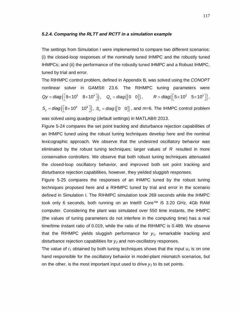
117

5.2.4. Comparing the RLTT and RCTT in a simulation example

The settings from Simulation I were implemented to compare two different scenarios:

(i) the closed-loop responses of the nominally tuned IHMPC and the robustly tuned

IHMPCs; and (ii) the performance of the robustly tuned IHMPC and a Robust IHMPC,

tuned by trial and error.

The RIHMPC control problem, defined in Appendix B, was solved using the CONOPT

nonlinear solver in GAMS® 23.6. The RIHMPC tuning parameters were

5 49 10 8 10Qy diag , 0 0uQ diag ,

2 35 10 5 10R diag ,

6 68 10 10yS diag , 0 0uS diag , and m=6. The IHMPC control problem

was solved using quadprog (default settings) in MATLAB® 2013.

Figure 5-24 compares the set point tracking and disturbance rejection capabilities of

an IHMPC tuned using the robust tuning techniques develop here and the nominal

lexicographic approach. We observe that the undesired oscillatory behavior was

eliminated by the robust tuning techniques; larger values of R resulted in more

conservative controllers. We observe that both robust tuning techniques attenuated

the closed-loop oscillatory behavior, and improved both set point tracking and

disturbance rejection capabilities, however, they yielded sluggish responses.

Figure 5-25 compares the responses of an IHMPC tuned by the robust tuning

techniques proposed here and a RIHMPC tuned by trial and error in the scenario

defined in Simulation I. The RIHMPC simulation took 269 seconds while the IHMPC

took only 6 seconds, both running on an Intel® Core™ i5 3.20 GHz, 4Gb RAM

computer. Considering the plant was simulated over 550 time instants, the IHMPC

(the values of tuning parameters do not interfere in the computing time) has a real

time/time instant ratio of 0.019, while the ratio of the RIHMPC is 0.489. We observe

that the RIHMPC yields sluggish performance for y1, remarkable tracking and

disturbance rejection capabilities for y2 and non-oscillatory responses.

The value of r1 obtained by both tuning techniques shows that the input u1 is on one

hand responsible for the oscillatory behavior in model-plant mismatch scenarios, but

on the other, is the most important input used to drive y1 to its set points.

118

Figure 5-24: Responses of the IHMPC tuned with RLTT (── ), RCTT ( ) and

LTT ( ). Set points and input bounds ( ).

119

Figure 5-25: C3/C4 splitter Simulation I. IHMPC with RLTT (── ), RCTT ( ) and a RIHMPC ( ). Set points and input bounds ( ).

120

In order to further investigate how the robust tuning techniques perform compared to

the robust controller, we propose another scenario, named Simulation II. The initial

conditions are 0 3000 1800 Tu , 0 0.9 50 Ty , the time instants at which the set

points are changed and its values are given in Table 5-24. The nominal model is

model 6, the plant model starts with model 6, changes to model 1 at 100 min, to

model 3 at 1200 min and to model 4 at 3100 min. The simulation runs for 7000

minutes.

Table 5-24: C3/C4 Simulation II set points. Time (min) ysp

1 (%) ysp2 (°C)

0 1 50 1000 0.95 49 3000 0.95 48.5 5000 0.9 48.5

Figure 5-26 show the results of Simulation II. We observe that the RIHMPC has an

overall better performance for y2 than the robustly tuned controller, although it yields

poor tracking capabilities for the set point of y1, it is more sluggish than the RLTT

IHMPC. The RCTT yields oscillatory behavior for both outputs, from 3000 to 4000

min, when the plant is represented by plant model 4. Figure 5-27 shows the output

responses for the set point change from time 1000 min until 1500 min. It is observed

that the IHMPCs tuned with the robust techniques yield oscillatory for output y1,

however, the response of the RIHMPC is sluggish and it takes almost 1000 minutes

to drive y1 to its set point. However, the RIHMPC response for y2 is faster and

smoother than the responses of the robustly tuned IHMPCs. The IHMPC tuned with

the robust compromise technique yields large amplitude oscillations whereas the

lexicographic technique yields a controller with low amplitude oscillations.

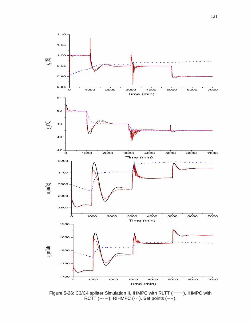
121

Figure 5-26: C3/C4 splitter Simulation II. IHMPC with RLTT (── ), IHMPC with RCTT ( ), RIHMPC ( ). Set points ( ).

122

Figure 5-27: Simulation II from 1000 min to 1500 min. IHMPC with RLTT (── ), IHMPC with RCTT ( ), RIHMPC ( ). Set points ( ).

123

The input profiles calculated by the nominal controllers were similar, except that the

compromise technique yields larger and more aggressive control moves. The

RIHMPC profiles, on the other hand, are smoother but tend to take much time to

reach the steady state. The trial and error tuning of the RIHMPC yielded a set of

tuning parameters that allows a better tracking performance of y2. When the value of

qy,1 is increased, the system response becomes oscillatory, especially when the plant

model is model 1.

The results shown here indicate that because of the sluggish responses of the

RIHMPC, it tends to oscillate less than the robustly tuned IHMPCs. However, the

computational time of the robust IHMPC is at least one order of magnitude larger

than the computational time of the robustly tuned controllers, for this relatively small

system. Regarding the nominal MPC implemented in the mismatch scenario, the

robustly tuned controller reduces oscillation and improves set point tracking and

disturbance rejection capabilities.

124

6. FINAL CONSIDERATIONS

6.1. Conclusions

The conclusions drawn from the case studies in this thesis are summarized here.

The FCC case study showed that the Lexicographic approach is more suitable for

systems in which ny=nu. It allows the calculation of appropriate tuning parameters to

achieve the best performance of the prioritized outputs in reasonable time, while a

trial and error tuning approach would take a lot of computer time. Also, this case

study unveils the flexibility of the technique to account for different goal definitions.

Even though the Lexicographic technique is able to respect output priority, and in real

application, there are as many degrees of freedom as the system inputs to define the

subsystem pairs, the method may still require much heuristics or fail to address

systems with ny≠nu straightforwardly.

The HOF case study showed that the proposed techniques lead to different values of

the corresponding optimum tuning parameters. The Lexicographic technique follows

the usual tuning guidelines of the industry, in which the goals are defined according

to the number of available inputs as degrees of freedom. The Lexicographic method

showed to be more suitable for systems in which the number of outputs is equal to

the number of inputs, whereas the compromise approach can take into account as

many objectives as necessary and is independent of the size of the system. The

lexicographic method successfully prioritizes the more important objectives, whereas

the Compromise method obtains the best attainable performance considering all

objectives simultaneously.

A MPC with output zone control and input targets was tuned using the compromise

approach in the CDU case study. The method was compared to a similar multi-

objective tuning approach, based on an a posteriori solution. The latter was, in

average, 22 times more expensive in terms of computational time than the proposed

method, which may result in an even more remarkable difference for large scale

systems, although both methods are carried out off-line. Two different strategies

were assessed: in the first strategy (Scenario II-A), matrices Qy and R are tuned in a

first step, considering the output tracking goals and in the second step, matrix Qu is

tuned, assuming that the optimum values of Qy and R are inherited from the previous

125

step and the input tracking goals are addressed. The second tuning strategy

(Scenario II-B) considers the case in which Qy, Qu and R are tuned considering the

input and output tracking goals simultaneously. In both strategies, typical operating

scenarios of the CDU are defined, in which an output is assumed to act as an active

constraint to an input reference trajectory tracking. The results showed that the

methodology defined in Scenario II-A might lead to fast but oscillatory responses. A

simulation study was performed, considering the output zones and input targets

defined in a real operating scenario of the CDU. The results showed that the

compromise method yielded similar responses to the existing set of tuning

parameters that were obtained by trial and error. The input tracking capability of the

latter was more efficient, but the former yielded better results in the output tracking

scenario analysis. Nonetheless, the trial and error approach, used to obtain the

existing tuning parameters, is cumbersome and time consuming and therefore,

should be used as a supplementary tuning method, instead of in the early stages of

the MPC tuning procedure.

In the last case study, we considered the C3/C4 splitter model, but with multi-plant

model uncertainty and assessed the robust formulations of the tuning techniques.

The analysis of the robust tuning results indicates which models are most different

from the nominal model, as well as what outputs are most likely to render the system

unstable. A robustly tuned IHMPC was compared to a RIHMPC in two scenarios. In

the first one, setpoint changes, plant model changes and unmeasured disturbances

take place in short time intervals. The simulation showed that the RIHMPC, although

much smoother than the robustly tuned IHMPC, was considerably more sluggish in

some conditions while the robust tuning techniques were able to find a compromise

between robustness and performance, through the inclusion of either a cost

contracting constraints (RLTT) or min-max optimization (RCTT). In the second

scenario, in which the time intervals between setpoint changes and plant model

changes are larger, in general the RIHMPC performed better than the robustly tuned

controllers. Oscillatory response for some plant models and large overshoot in

disturbance rejection were the main drawbacks from the latter. However, we kept

track of the simulation time and compared how long the RIHMPC and IHMPC take to

complete the 550 time instants simulation. The robust controller about 0.489

sec/iteration while the robust tuned controller took about 0.019 sec/iteration. The

difference, which is over one order of magnitude, might not be significant for a small

126

system as the C3/C4 splitter, however, time is crucial in industrial applications of

MPCs, and RIHMPCs have been questioned due to their computational expense.

Robust tuning techniques for nominal controllers might address this problem by

shifting the heavy computational burden to offline applications. The simulation results

indicate that tuning an existing controller for a different scenario might be a cheap

solution to improve its performance. In certain circumstances, the financial cost

involved in the project and commissioning of a new control platform is prohibiting, but

a simple change in the tuning parameters of the existing controller might yield a profit

increase due to less oscillatory responses.

6.2. Directions for further work

A major limitation for industrial application of the tuning techniques developed here is

the lack of knowledge about model uncertainty, which highly affect the system

operation over long time intervals, due to equipment deterioration; or over short

intervals, due to changes in operational points, and system disturbances. Properly

identifying a set of models, over a significant range of operating conditions is almost

impossible or, at least not practical and cumbersome from a practical point of view.

From the findings in this thesis, robust tuning techniques seem a valid alternative for

robust predictive controllers, under the assumption that the user is able to provide a

reliable uncertainty representation. Therefore, two suggestions are due: first,

alternatives for model identification in different conditions and operational points

should be developed. Second, online tuning techniques, on one hand capable of

dealing with model uncertainty based on a database of previous control actions and

system behavior, and on the other, fast enough to run and optimize tuning

parameters once model mismatch is detected. These are interesting alternatives for

the current industrial needs.

Moreover, a straightforward extension of the tuning methods proposed here for

robust MPC is also a possibility.

127

REFERENCES

Abbas, A., & Sawyer, P. E. (1995). A multiobjective design algorithm: Application to

the design of siso control systems. Computers & Chemical Engineering, 19(2),

241–248.

Abu-Ayyad, M., Dubay, R., & Kember, G. (2006). SISO extended predictive control—

formulation and the basic algorithm. ISA Transactions, 45(1), 9–20.

Adam, E. J., & Marchetti, J. L. (2004). Designing and tuning robust feedforward

controllers. Computers & Chemical Engineering, 28(9), 1899–1911.

Al-Ghazzawi, A., Ali, E., Nouh, A., & Zafiriou, E. (2001). On-line tuning strategy for

model predictive controllers. Journal of Process Control, 11(3), 265–284.

Ali, E., & Zafiriou, E. (1993a). On the tuning of nonlinear model predictive control

algorithms. In Proceedings of the 1993 American Control Conference, Vols. 1-3

(pp. 786–790).

Ali, E., & Zafiriou, E. (1993b). Optimization-based tuning of nonlinear model

predictive control with state estimation. Journal of Process Control, 3(2), 97–107.

Alvarez, L. A., Francischinelli, E. M., Santoro, B. F., & Odloak, D. (2009). Stable

Model Predictive Control for Integrating Systems with Optimizing Targets.

Industrial & Engineering Chemistry Research, 48(20), 9141–9150.

Banerjee, P., & Shah, S. L. (1992). Tuning guidelines for robust generalized

predictive control. In Proceedings of the 31st IEEE Conference on Decision and

Control (pp. 3233–3234). IEEE.

Bauer, M., & Craig, I. K. (2008). Economic assessment of advanced process control

– A survey and framework. Journal of Process Control, 18(1), 2–18.

Bemporad, A., & Morari, M. (1999). Control of systems integrating logic, dynamics,

and constraints. Automatica, 35(3), 407–427.

128

Bemporad, A., & Muñoz de la Peña, D. (2009). Multiobjective model predictive

control. Automatica, 45(12), 2823–2830.

Bequette, B. W. (1991). Nonlinear control of chemical processes: a review. Industrial

& Engineering Chemistry Research, 30(7), 1391–1413.

Bristol, E. (1966). On a new measure of interactions for multivariable process control.

Automatic Control, IEEE Transactions on, 11(1), 133–134.

Cairano, S. Di, & Bemporad, A. (2009). Model predictive controller matching: Can

MPC enjoy small signal properties of my favorite linear controller? In European

Control Conference, Budapest, Hungary, 23th -26th.

Cairano, S. Di, & Bemporad, A. (2010). Model Predictive Control Tuning by Controller

Matching. IEEE Transactions on Automatic Control, 55(1), 185–190.

Campi, M. C., Lecchini, A., & Savaresi, S. M. (2002). Virtual reference feedback

tuning: a direct method for the design of feedback controllers. Automatica, 38(8),

1337–1346.

Cannon, M., Kouvaritakis, B., & Wu, X. (2009). Model predictive control for systems

with stochastic multiplicative uncertainty and probabilistic constraints.

Automatica, 45(1), 167–172.

Chatterjee, T., & Saraf, D. N. (2004). On-line estimation of product properties for

crude distillation units. Journal of Process Control, 14(1), 61–77.

Das, I., & Dennis, J. E. (1998). Normal-Boundary Intersection: A New Method for

Generating the Pareto Surface in Nonlinear Multicriteria Optimization Problems.

SIAM Journal on Optimization, 8(3), 631–657.

Exadaktylos, V., & Taylor, C. J. (2010). Multi-objective performance optimisation for

model predictive control by goal attainment. International Journal of Control,

83(7), 1374–1386.

129

Francisco, M., Alvarez, H., Vega, P., & Revollar, S. (2010). Stable Model Predictive

Control tuning considering asymmetric bounded signals. In 20th European

Symposium on Computer Aided Process Engineering (pp. 493–498).

Francisco, M., & Vega, P. (2010). Automatic tuning of model predictive controllers

based on multiobjective optimization. Latin American Applied Research, 40,

255–265.

Francisco, M., Vega, P., & Revollar, S. (2011). Model Predictive Control of BSM1

benchmark of wastewater treatment process: A tuning procedure. In IEEE

Conference on Decision and Control and European Control Conference (pp.

7057–7062). IEEE.

Froisy, J. B. (2006). Model predictive control—Building a bridge between theory and

practice. Computers & Chemical Engineering, 30(10-12), 1426–1435.

Gambier, A. (2008). MPC and PID control based on Multi-Objective Optimization. In

2008 American Control Conference (pp. 4727–4732). IEEE.

Garcia, C. E., & Morari, M. (1982). Internal model control. A unifying review and

some new results. Industrial & Engineering Chemistry Process Design and

Development, 21(2), 308–323.

Garcia, C. E., Prett, D. M., & Morari, M. (1989). Model predictive control: Theory and

practice—A survey. Automatica, 25(3), 335–348.

Garriga, J. L., & Soroush, M. (2008). Model predictive controller tuning via eigenvalue

placement. In 2008 American Control Conference (pp. 429–434). IEEE.

Garriga, J. L., & Soroush, M. (2010). Model Predictive Control Tuning Methods: A

Review. Industrial & Engineering Chemistry Research, 49(8), 3505–3515.

Georgiou, A., Georgakis, C., & Luyben, W. L. (1988). Nonlinear dynamic matrix

control for high-purity distillation columns. AIChE Journal, 34(8), 1287–1298.

130

Geyer, T., Papafotiou, G., & Morari, M. (2009). Model Predictive Direct Torque

Control—Part I: Concept, Algorithm, and Analysis. IEEE Transactions on

Industrial Electronics, 56(6), 1894–1905.

Giovanini, L., & Marchetti, J. L. (1999). Shaping Time-Domain Responses with

Discrete Controllers. Industrial & Engineering Chemistry Research, 38(12),

4777–4789.

Grosdidier, P., Mason, A., Aitolahti, A., Heinonen, P., & Vanhamäki, V. (1993). FCC

unit reactor-regenerator control. Computers & Chemical Engineering, 17(2),

165–179.

Han, K., Zhao, J., & Qian, J. (2006). A Novel Robust Tuning Strategy for Model

Predictive Control. 2006 6th World Congress on Intelligent Control and

Automation, 6406–6410.

Huusom, J. K., Poulsen, N. K., Jørgensen, S. B., & Jørgensen, J. B. (2012). Tuning

SISO offset-free Model Predictive Control based on ARX models. Journal of

Process Control, 22(10), 1997–2007.

J.M. Maciejowski. (2002). Predictive control with constraints. International Journal of

Adaptive Control and Signal Processing (Vol. 17). London: Prentice Hall.

Júnior, G. A. N., Martins, M. A. F., & Kalid, R. (2014). A PSO-based optimal tuning

strategy for constrained multivariable predictive controllers with model

uncertainty. ISA Transactions, 53, 560–567.

Kerrigan, E. C., Bemporad, A., Mignone, D., Morari, M., & Maciejowski, J. M. (2000).

Multi-objective prioritisation and reconfiguration for the control of constrained

hybrid systems. In Proceedings of the 2000 American Control Conference. ACC

(IEEE Cat. No.00CH36334) (Vol. 3, pp. 1694–1698). American Autom. Control

Council.

Kerrigan, E. C., & Maciejowski, J. M. (2002). Designing model predictive controllers

with prioritised constraints and objectives. In Proceedings. IEEE International

Symposium on Computer Aided Control System Design (pp. 33–38). IEEE.

131

Kulhavy, R., Lu, J., & Samad, T. (2001). Emerging technologies for enterprise

optimization in the process industry (pp. 411–422). Tucson, Arisona.

Lee, J. H., Morari, M., & Garcia, C. E. (1994). State-space interpretation of model

predictive control. Automatica, 30(4), 707–717.

Lee, J. H., & Yu, Z. H. (1994). Tuning of model predictive controllers for robust

performance. Computers & Chemical Engineering, 18(1), 15–37.

Lee, K. H., Huang, B., & Tamayo, E. C. (2008). Sensitivity analysis for selective

constraint and variability tuning in performance assessment of industrial MPC.

Control Engineering Practice, 16(10), 1195–1215.

Li, S., & Du, G. (2002). Online tuning scheme for generalized predictive controller via

simulation-optimization. In 2002 IEEE World Congress on Computational

Intelligence. 2002 IEEE International Conference on Fuzzy Systems. FUZZ-

IEEE’02. Proceedings (Cat. No.02CH37291) (Vol. 2, pp. 1381–1386). IEEE.

Li, S., Zhang, Y., & Zhu, Q. (2005). Nash-optimization enhanced distributed model

predictive control applied to the Shell benchmark problem. Information Sciences,

170(2-4), 329–349.

Liau, L. C.-K., Yang, T. C.-K., & Tsai, M.-T. (2004). Expert system of a crude oil

distillation unit for process optimization using neural networks. Expert Systems

with Applications, 26(2), 247–255.

Liu, W., & Wang, G. (2000). Auto-tuning procedure for model-based predictive

controller. In SMC 2000 Conference Proceedings. 2000 IEEE International

Conference on Systems, Man and Cybernetics. “Cybernetics Evolving to

Systems, Humans, Organizations, and their Complex Interactions” (Cat.

No.00CH37166) (Vol. 5, pp. 3421–3426). IEEE.

Luo, Y., Wang, H., & Yuan, X. (2013). Simultaneous optimization for heat-integrated

crude oil distillation system. In Proceedings of the 6th International Conference

on Process System Engineering (PSE ASIA) (pp. 25–27). Kuala Lumpur.

132

Maciejowski, J. M. (2002). Predictive Control: With Constraints (p. 331). Prentice

Hall.

Marchetti, J. L., Mellichamp, D. A., & Seborg, D. E. (1983). Predictive control based

on discrete convolution models. Industrial & Engineering Chemistry Process

Design and Development, 22(3), 488–495.

Martins, M. A. F., Yamashita, A. S., Santoro, B. F., & Odloak, D. (2013). Robust

model predictive control of integrating time delay processes. Journal of Process

Control, 23(7), 917–932.

MATLAB. (2013). version 8.1.0.604 (2013a). Natick, Massachusetts: The MathWorks

Inc.

Maurath, P. R., Laub, A. J., Seborg, D. E., & Mellichamp, D. A. (1988). Predictive

controller design by principal components analysis. Industrial & Engineering

Chemistry Research, 27(7), 1204–1212.

Messac, A. (1996). Physical programming - Effective optimization for computational

design. AIAA Journal, 34(1), 149–158.

Messac, A., & Wilsont, B. (1998). Physical Programming for Computational Control.

AIAA Journal, 36(2), 219–226.

Mizoguchi, A., Marlin, T. E., & Hrymak, A. N. (1995). Operations optimization and

control design for a petroleum distillation process. The Canadian Journal of

Chemical Engineering, 73(6), 896–907.

Morari, M., & Lee, J. H. (1999). Model predictive control : past , present and future.

Process Engineering, 23, 667–682.

Oliveira, J. B., Boaventura-Cunha, J., Moura Oliveira, P. B., & Freire, H. (2014). A

swarm intelligence-based tuning method for the sliding mode generalized

predictive control. ISA Transactions.

133

Pohekar, S. D., & Ramachandran, M. (2004). Application of multi-criteria decision

making to sustainable energy planning—A review. Renewable and Sustainable

Energy Reviews, 8(4), 365–381.

Porfírio, C. R., Almeida Neto, E., & Odloak, D. (2003). Multi-model predictive control

of an industrial C3/C4 splitter. Control Engineering Practice, 11(7), 765–779.

Qin, S. J., & Badgwell, T. A. (2003). A survey of industrial model predictive control

technology. Control Engineering Practice, 11(7), 733–764.

Rani, K. Y., & Unbehauen, H. (1997). Study of Predictive Controller Tuning Methods.

Automatica, 33(12), 2243–2248.

Reynoso-Meza, G., Garcia-Nieto, S., Sanchis, J., & Blasco, F. X. (2013). Controller

Tuning by Means of Multi-Objective Optimization Algorithms: A Global Tuning

Framework. IEEE Transactions on Control Systems Technology, 21(2), 445–

458.

Rojas, C. A., Rodriguez, J., Villarroel, F., Espinoza, J. R., Silva, C. A., & Trincado, M.

(2013). Predictive Torque and Flux Control Without Weighting Factors. IEEE

Transactions on Industrial Electronics, 60(2), 681–690.

Santoro, B. F., & Odloak, D. (2012). Closed-loop stable model predictive control of

integrating systems with dead time. Journal of Process Control, 22(7), 1209–

1218.

Sarhadi, P., Salahshoor, K., & Khaki-Sedigh, A. (2012). Robustness analysis and

tuning of generalized predictive control using frequency domain approaches.

Applied Mathematical Modelling, 36(12), 6167–6185.

Seo, J. W., Oh, M., & Lee, T. H. (2000). Design Optimization of a Crude Oil

Distillation Process. Chemical Engineering & Technology, 23(2), 157–164.

Shah, G., & Engell, S. (2010). Tuning MPC for desired closed-loop performance for

SISO systems. In 18th Mediterranean Conference on Control and Automation,

MED’10 (pp. 628–633). IEEE.

134

Shah, G., & Engell, S. (2011). Tuning MPC for desired closed-loop performance for

MIMO systems. In American Control Conference (ACC), 2011 (pp. 4404 – 4409).

Shridhar, R., & Cooper, D. J. (1997). A Tuning Strategy for Unconstrained SISO

Model Predictive Control. Ind. Eng. Chem. Res., 36, 729–746.

Shridhar, R., & Cooper, D. J. (1998). A Tuning Strategy for Unconstrained

Multivariable Model Predictive Control. Ind. Eng. Chem. Res., 5885(98), 4003–

4016.

Subbu, R., Bonissone, P., Eklund, N., Yan, W., Iyer, N., Xue, F., & Shah, R. (2006).

Management of Complex Dynamic Systems based on Model-Predictive Multi-

objective Optimization. In 2006 IEEE International Conference on Computational

Intelligence for Measurement Systems and Applications (pp. 64–69). IEEE.

Susuki, R., Kawai, F., Nakazawa, C., Matsui, T., & Aiyoshi, E. (2008). Parameter

Optimization of Model Predictive Control Using PSO. In SICE Annual

Conference (pp. 1981–1988).

Susuki, R., Kawai, F., Nakazawa, C., Matsui, T., & Aiyoshi, E. (2012). Parameter

optimization of model predictive control by PSO. Electrical Engineering in Japan,

178(1), 40–49.

Trierweiler, J. O., & Farina, L. a. (2003). RPN tuning strategy for model predictive

control. Journal of Process Control, 13(7), 591–598.

Vallerio, M., van Impe, J., & Logist, F. (2014). Tuning of NMPC controllers via multi-

objective optimisation. Computers & Chemical Engineering, 61, 38–50.

van de Wal, M., & de Jager, B. (2001). A review of methods for input/output

selection. Automatica, 37(4), 487–510.

van der Lee, J. H., Svrcek, W. Y., & Young, B. R. (2008). A tuning algorithm for

model predictive controllers based on genetic algorithms and fuzzy decision

making. ISA transactions, 47(1), 53–9.

135

Vega, P., Francisco, M., & Sanz, E. (2007). Norm based approaches for automatic

tuning of Model Based Predictive Control. In Proceedings of European Congress

of Chemical Engineering ECCE-6.

Vega, P., Francisco, M., & Tadeo, F. (2008). Multiobjective optimization for automatic

tuning of robust Model Based Predictive Controllers. In Proceedings of the 17th

World Congress - The International Federation of Automatic Control (pp. 6980–

6985).

Villarroel, F., Espinoza, J., Rojas, C., Molina, C., & Espinosa, E. (2010). A

multiobjective ranking based finite states model predictive control scheme

applied to a direct matrix converter. In IECON 2010 - 36th Annual Conference on

IEEE Industrial Electronics Society (pp. 2941–2946). IEEE.

Wojsznis, W., Gudaz, J., Blevins, T., & Mehta, A. (2003). Practical approach to tuning

MPC. ISA Transactions, 42(1), 149–162.

Zavala, V. M., & Flores-Tlacuahuac, A. (2012). Stability of multiobjective predictive

control: A utopia-tracking approach. Automatica, 48(10), 2627–2632.

136

APPENDIX A – Transfer function for the case studies

Fluid Catalytic Cracking

Table A1: FCC Reactor Regenerator. u1 u2

y1 3 2

0.8713 17.9 5.9 1s s s

4 3 2

0.023 0.0926.29 15.76 15.27 6.8 1

ss s s s

y2 3 2

0.5527 35.7 9.7 1s s s

4 3 2

0.5517 29.33 21.99 7 1s s s s

y3 3 2

0.2517 24 8 1s s s

3 2

0.255.1 8 5.1 1s s s

y4 3 2

0.01446 54.5 9.5 1s s s

4 3 2

0.1478.2 111.1 65.55 10.6 1s s s s

u3 u4

y1

2

4 3 20.2273 0.4026 0.074

120.9 109 46.1 10 1s s

s s s s

2

0.4840 14 1

ss s

y2

2

4 3 20.8051 1.732 0.74

143 171.9 75.1 14.3 1s s

s s s s

20.36

33 6.5 1s s

y3 3 2

0.448 0.739 34 10 1

ss s s

2

0.4977 0.07924 12.01 1

ss s

y4

2

4 3 22.765 4.493 0.27

689 670 227 30 1s s

s s s s

2

0.18 0.01566 27 1

ss s

137

C3/C4 Splitter

Transfer function model

,, ,0 , ,1

2, ,1 , ,2

,1

i jsi j i j

i j i j

b b s eGi j s

a s a s A-1

Figure A1: Operating range and operational points of the C3/C4 splitter (Adapted

from Porfítio, Neto and Odloak, 2003).

Table A2: C3/C4 transfer function coefficients. (i,j) b0 b1 a1 a2 θ

Operating point 1

(1,1) 1.09E-05 4.23E-05 1.09E-01 2.43E-02 0

(1,2) -3.82E-05 -1.21E-04 1.34E-01 2.43E-02 0

(2,1) -1.12E-04 -8.73E-05 1.32E-01 7.30E-03 0

(2,2) 7.00E-03 1.30E-03 2.26E+00 1.37E-01 0

Operating point 2

(1,1) 4.22E-04 -2.72E-04 1.66E+00 2.53E-01 0

138

(1,2) -1.41E-04 -2.18E-04 1.32E-01 1.17E-02 0

(2,1) -6.30E-03 -3.40E-03 2.07E+00 2.43E-01 0

(2,2) 4.50E-03 2.00E-04 8.35E-01 8.12E-02 0

Operating point 3

(1,1) 1.53E-03 -8.60E-04 1.19E+00 9.12E-02 0

(1,2) -7.81E-04 -3.77E-04 3.40E-01 1.81E-02 0

(2,1) -8.00E-04 -3.40E-03 4.02E-01 3.65E-02 0

(2,2) 8.90E-03 6.40E-03 1.90E+00 1.95E-01 0

Operating point 4

(1,1) 4.88E-04 -1.11E-04 9.88E-01 6.46E-02 0

(1,2) -1.86E-04 -1.76E-04 2.61E-01 9.10E-03 0

(2,1) -2.50E-03 -3.90E-03 8.87E-01 8.40E-02 0

(2,2) 2.90E-03 5.50E-03 8.60E-01 3.92E-02 0

Operating point 5

(1,1) 5.65E-04 -3.54E-04 8.17E-01 -8.09E-02 0

(1,2) -4.78E-04 -1.43E-04 3.42E-01 2.59E-02 0

(2,1) -2.10E-03 -1.90E-03 1.17E+00 1.07E-01 0

(2,2) 8.10E-03 5.30E-03 2.42E+00 1.76E-01 0

Operating point 6

(1,1) 5.66E-04 -2.22E-04 3.49E+00 5.90E-01 0

(1,2) -1.45E-03 7.41E-05 2.70E+00 4.02E-01 0

(2,1) -1.24E-03 -1.14E-03 1.64E+00 9.85E-02 0

(2,2) 2.00E-03 -3.00E-04 2.43E+00 6.51E-02 0

139

Crude Distillation Unit

The omitted entries in Table A4 represent null transfer functions.

Table A4: CDU. u1

y8

4 5 3 4 2 3 3 2 3 4

6 5 4 3 2 4

7.31 10 1.82 10 1.49 10 2.67 10 1.32 10 1.71 102.18 5.83 2.14 0.56 0.03 9.07 10

s s s s ss s s s s s

y9

2 6 5 4 3 2 3 4

7 6 5 4 3 2 3

2.63 10 0.17 0.36 0.15 0.12 5.55 10 8.86 108.16 29.45 19.87 7.98 1.11 0.10 3.20 10

s s s s s ss s s s s s s

y10

4 5 4 4 4 3 5 2 5 5

6 5 4 3 2 3

1.88 10 1.11 10 1.53 10 8.67 10 1.76 10 3.90 103.83 6.67 2.84 0.68 0.12 4.88 10

s s s s ss s s s s s

u2

y3

2

3 2

1.29 1.37 2.131.99 0.99 0.19

s ss s s

y7

3 32

3 2 3

4.60 0.06 4.110.39 0.010 10

17 02.93s s

s s s

y8

6 5 4 3 2

7 6 5 4 3 211.31 102.90 58.29 171.20 362.10 159.70 56.27

8.84 38.89 71.07 83.25 53.24 19.11 3.16s s s s s s

s s s s s s s

y9

5 4 3 2

6 5 4 3 2 38.80 13.69 8.60 5.95 0.89 0.18

4.13 4.94 2.19 0.65 0.11 7.57 10s s s s s

s s s s s s

y10

3 2 4 4

3 2 34.67 10 5.59 10 6.76 10

0.32 0.06 5.19 10s s

s s s

u3

y1

3 2

4 3 20.46 1.15 7.40 0.91

2.57 11.90 3.96 0.32s s s

s s s s

y7

3 2

4 3 20.20 1.08 3.67 3.139.85 35.88 12.34 1.62

s s ss s s s

y8

2

3 20.83 15.19 4.86

1.85 0.46 0.06s s

s s s

y9

2

3 20.56 14.74 5.08

1.96 0.52 0.05s s

s s s

140

y10

3 3 2

4 3 21.82 10 0.20 0.41 0.78

3.55 14.10 9.24 2.22s s s

s s s s

u4

y2

6 5 4 3 2

7 6 5 4 3 2 3

0.24 0.14 1.71 3.63 3.72 0.66 0.055.58 19.65 39.65 11.93 3.85 0.20 4.13 10

s s s s s ss s s s s s s

y3

5 4 3 2

6 5 4 3 2

0.14 3.82 7.56 12.02 0.30 0.395.22 18.97 17.63 3.14 0.32 0.01

s s s s ss s s s s s

y4

2

3 20.13 0.26 0.29

4.16 1.90 0.32s s

s s s

y5

4 6 5 4 3 2 3

7 6 5 4 3 26.42 10 0.02 0.04 0.05 0.04 0.03 6.327 10

4.27 16.04 10.95 6.98 1.72 0.51 0.02s s s s s s

s s s s s s s

y6

3 2

4 3 20.03 0.12 0.60 0.42

3.26 13.41 7.94 1.64s s s

s s s s

u5

y5

2 4 4 4

3 2 36.499 10 6.382 10 1.923 10

0.58 0.09 5.371 10s s

s s s

u6

y3

3 2

4 3 20.05 0.52 1.92 2.324.56 17.19 17.01 5.58

s s ss s s s

y4

3 2

4 3 2

0.01 0.03 0.05 0.447.28 29.63 53.21 33.54

s s ss s s s

y6

4 2 5 4

3 2

9.46 10 1.39 10 1.72 100.46 0.12 0.01

s ss s s

u7

y2

5 4 3 2 4 4

6 5 4 3 2 40.01 0.02 0.02 0.01 1.84 10 1.89 10

3.39 4.97 2.45 0.47 0.03 9.58 10s s s s s

s s s s s s

y3

3 2 4 4

3 2 41.84 10 6.35 10 1.07 10

0.26 0.02 3.83 10s s

s s s

y4

4 3 3 3 2 4 5

5

4

4 3 2 36.67 1.26 10 1.71 10 1.68 10 6.58 10

2.48 3.34 0.66 0.08 4.090

101s s s ss s s s s

141

y5

4 5 4 4 4 3 5 2 6 8

6 5 4 3 2 4 638.51 10 1.52 10 1.48 10 1.01 10 1.32 10 6. 10

0.31 0.21 0.04 6.14 2.93 10 5.26 1010s s s s s

s s s s s s

y6

4 3 5 2 3

4 3 28.431 10 5.02 10 0.02 3.67 10

3.34 13.05 3.09 0.25s s s

s s s s

u8

y3

6 5 4 3 2

7 6 5 4 3 2

0.5407 1.312 0.5546 0.3327 0.06388 0.005414 0.00031310.4485 0.599 0.1516 0.06437 0.009542 0.0005524 1.289 05

s s s s s ss s s s s s s e

y4

3 2

4 3 20.008947 0.3574 1.39 0.9825

4.132 15.16 7.629 1.396s s s

s s s s

y5

5 4 3 2

6 5 4 3 20.02 0.26 0.74 0.21 0.11 0.045.85 20.46 13.84 4.03 0.67 0.04

s s s s ss s s s s s

y10

3 2

4 3 20.03 0.10 0.51 0.11

2.96 12.66 5.60 0.70s s s

s s s s

142

APPENDIX B – MPC formulations

DMC Controller

Industry has accepted Dynamic Matrix Control (DMC), formalized in (Cutler &

Ramaker, 1980), as a standard advanced control strategy because it

straightforwardly includes process constraints in the control problem. It is applicable

to both MIMO and SISO systems. The DMC is based on a step-response or an

impulse-response model, which are more intuitive than the state-space models.

Model Representation

In a SISO system, an output impulse response is represented by (B-1).

1

,ii

y k h u k i (B-1)

ih is a sampled output when the system is excited by a unitary impulse, u k and

y k are the input and output values at time instant k.

It is assumed that the impulse response is asymptotically stable and the model

horizon, N, is defined as the upper bound on the impulse response horizon. The

output prediction, ˆ |y k j k , at time instant k+j, calculated using system information

available at time instant k, is defined in (B-2).

1

ˆ | |N

ii

y k j k h u k j i k (B-2)

It is easy to write (B-2) using a step response model representation. The difference

between the two representations is the characteristic of the input signal; in the step

response model it is a step perturbation. The truncated step response at time step k

is shown in (B-3).

143

01

,N

ii

y k y g u k i (B-3)

where 0y is the output reference value that can be set to 0 without loss of generality,

ig is the sampled output value when the system is excited by an unitary step and

1u k u k u k . The output prediction at time instant k+j, for SISO systems,

is calculated as follows:

1

ˆ | |N

ii

y k j k g u k j i k (B-4)

and the following relationships hold:

1

, 1 ,,i

i jj

g h i N (B-5)

1, , ,1i i ih g g i N (B-6)

Equations (B-5) and (B-6) show the relationships between the impulse and step

responses coefficients.

Assuming that the system disturbances are constant until time step k+N, the

prediction error is represented in (B-7) and the predicted output value is calculated as

the sum of the system free response and the input contribution, according to (B-8).

ˆ ˆ ˆ| | ,| , 1,n k i k n k k y k y k k i N (B-7)

1 1

1 1 1

1

ˆˆ | |

,

i N

j jj j i

i N N

j j jj j i j

i

jj

y k i k g u k i j g u k i j n k i k

g u k i j g u k i j y k g u k j

g u k i j f k i

(B-8)

144

f k i is the system free response at time instant k+i; the part of the system

response that does not depend on the future control actions. Since the system is

assumed to be asymptotically stable, 1 0,j jg g j N .

In the right hand side of (B-8), the first term contains the effects of future control

actions, the second term contains the effects of the past control actions (which are

known and already implemented into the system) and the last term represents the

constant disturbances, according to (B-9).

1

N

j i jj

f k i y k g g u k j (B-9)

Then, the output predictions along the prediction horizon, considering m control

actions in the future, are calculated as follows:

1

2 1

1

ˆ 1| 1ˆ 2 | 1 2

ˆ |p

ii p m

y k k g u k f ky k k g u k g u k f k

y k p k g u k p i f k p

(B-10)

It is convenient to define the system dynamic matrix, mD , arranging the step

response coefficients as in (B-11) to write (B-10) in the compact form, seen in (B-12).

1

2 1

1 1

1 1

0 00

mm m

p p p m

gg g

Dg g g

g g g

(B-11)

cm ky D u f (B-12)

Equation (B-12) relates the predicted outputs to the control moves, and it will be used

to calculate the optimum input moves to track the output set-points.

145

The discussion above holds for MIMO systems. The model equations are extended

to accommodate the vectors and matrices of large dimensions. In a system with nu

inputs and ny outputs, the notation in (B-13) is used.

1 1

,nu N

lj lj i

l iy k h u k i (B-13)

ljih is the sampled value of output j at time instant i for an unitary impulse in input l,

j=1,…,ny; l=1,…,nu; i=1,…,N. Assuming model linearity, and using the superposition

principle, cy , ku and f are defined for MIMO systems according to (B-14), (B-15)

and (B-16)

1 11| 1| | |Tc

ny nyy y k k y k k y k p k y k p k (B-14)

1 1 1 1T

k nu nuu u k u k u k m u k m (B-15)

1 11| 1| | |T

ny nyf f k k f k k f k p k f k p k (B-16)

c ny py , nu m

ku , ny pf , ny p nu mmD and the MIMO dynamic matrix is

defined in (B-17).

1,1

2,1 12

,1 1,2 1,

0 0

0 ,m

p p p m nu

g

g gD

g g g

(B-17)

, , ; 1, ,, 1,i j p jg i nu are submatrices containing the coefficients ,i kg of the i-th

step response for the k-th output value corresponding to a step perturbation in the j-

th input.

Control Algorithm

146

The DMC cost function is calculated according to (B-18), and its control problem is

solved by minimizing (B-18) subject to the constraints defined in (B-19) and (B-20).

12 2

0 0

ˆmin ( ) ( ) ( )yk

p m

k sp RQui i

V y k i k y k i u k i k (B-18)

subject to

min max, 0, , 1u u k j u j m (B-19)

max max, 0, , 1u u k j u j m (B-20)

nyspy k i is the output set point, min

nuu , maxnuu are the lower and upper

bound of the inputs and maxnuu is the maximum allowed control move.

, 0ny nyy yQ Q and , 0nu nuR R are diagonal matrices. The problem is cast

as a QP, using (B-12). Assuming a constant output setpoint, spy k , the set point

vector is defined as

,sp sp ny psp sp

p

y y k y k y . Equation (B-12) can be

used to correlate the output prediction to the control actions, which are the decision

variables of the DMC control problem. Equations (B-19) and (B-20) can also be

written in terms of ku as follows:

| |0 01| 1|0

1

1| 1|0

|1|

, 1

1|

nu

nu nu

nu nu nu

nu nu nu

IM

k nu

u k k u k kI Iu k k u k kI I I

u k

u k m k u k m kI I I

u k ku k k

or M u I u k

u k m k

(B-21)

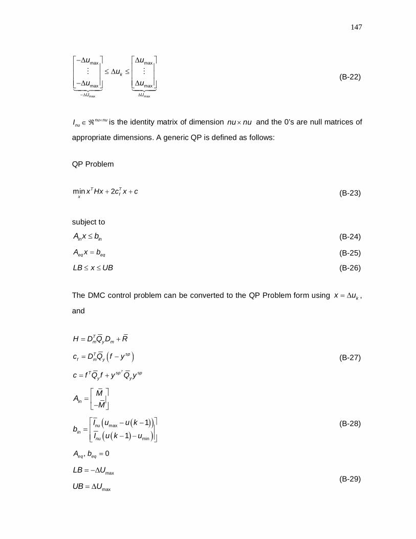
147

max max

max max

max max

k

U U

u uu

u u

(B-22)

nu nu

nuI is the identity matrix of dimension nu nu and the 0’s are null matrices of

appropriate dimensions. A generic QP is defined as follows:

QP Problem

min 2T Tfx

x Hx c x c (B-23)

subject to

in inA x b (B-24)

eq eqA x b (B-25)

LB x UB (B-26)

The DMC control problem can be converted to the QP Problem form using kx u ,

and

Tm y mH D Q D R

T spf m yc D Q f y

TT sp sp

y yc f Q f y Q y

(B-27)

inMAM

max

min

1

1nu

innu

I u u kb

I u k u

, 0eq eqA b

(B-28)

maxLB U

maxUB U (B-29)

148

where

y y y

p

Q blockdiag q q ,

m

R blockdiag r r .

The potential inconveniences of the DMC algorithm are the large dimension of the

step response model and the inability to cope with integrating systems.

The parameters that affect stability and performance in the DMC are the prediction

horizon (p), the control horizon (m), the model horizon (N), the sampling time (Ts),

and the cost function weighting matrices on the differences between predicted

outputs and their set points (Qy) and on the control moves (R).

MPC with input targets and zone control

The MPC studied here is based on the state-space model presented in (González &

Odloak, 2009). The MPC cost function takes into account the deviation between the

predicted system outputs, calculated using a state space system model over the

prediction horizon, and the output set points; the penalization of the input increments;

and the deviation between the system inputs and the input targets, both over the

control horizon. The MPC considered here is defined through the solution to the

following problem:

1 12 2 2

, ,, 1 0 0min | | |

uk sp

p m m

sp k des kR QQyu yi i i

y k i k y u k i k u k i k u

(B-30)

subject to the state space model of the system, the bounds on the inputs and input

increments ((B-19) and (B-20)) and

min , maxsp ky y y (B-31)

The parameter ,nu

des ku is an input target, assumed to be defined by an upper

layer of the control structure and ,ny

sp ky is the output set point that is an

additional decision variable of the control problem; assumed to be restricted within a

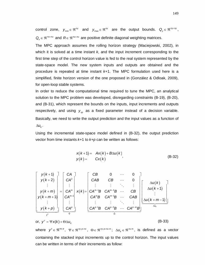
149

control zone, minnyy and max

nyy are the output bounds. ny nyyQ ,

nu nuuQ and nu nuR are positive definite diagonal weighting matrices.

The MPC approach assumes the rolling horizon strategy (Maciejowski, 2002), in

which it is solved at a time instant k, and the input increment corresponding to the

first time step of the control horizon value is fed to the real system represented by the

state-space model. The new system inputs and outputs are obtained and the

procedure is repeated at time instant k+1. The MPC formulation used here is a

simplified, finite horizon version of the one proposed in (González & Odloak, 2009),

for open-loop stable systems.

In order to reduce the computational time required to tune the MPC, an analytical

solution to the MPC problem was developed, disregarding constraints (B-19), (B-20),

and (B-31), which represent the bounds on the inputs, input increments and outputs

respectively, and using spy as a fixed parameter instead of a decision variable.

Basically, we need to write the output prediction and the input values as a function of

ku .

Using the incremental state-space model defined in (B-32), the output prediction

vector from time instants k+1 to k+p can be written as follows:

1

,x k Ax k B u ky k Cx k

(B-32)

2

1 2

1 1

1 2

1 0 02 0

1

c

m m m

m m m

p p p p m

y

y k CA CBy k CA CAB CB

y k m x kCA CA B CA B CBy k m CA CA B CA B CAB

y k p CA CA B CA B CA B

1

1ku

u ku k

u k m

or, ( )cky x k u (B-33)

where c ny py , ny p nx , ny p nu m ; nu mku , is defined as a vector

containing the stacked input increments up to the control horizon. The input values

can be written in terms of their increments as follow:

150

| 0 0 ( | )1| 0 ( 1| )

( 1)

1| ( 1| )c

k

nu nu

nu nu nu

nu nu nu nu nu

IM u nuu

u k k I Iu k ku k k I I Iu k k

u k

u k m k I I I I Iu k m k

(B-34)

or, ( 1)ck nuu M u I u k (B-35)

where c nu mu , nu m nu mM , nu m nunuI , nuI is a nu nu identity matrix. Finally,

the modified MPC control problem can be written in terms of ku using (B-34) and

(B-35).

2 22min ( 1)

y ukk ny sp k k nu nu desRQ Qu

x k u I y u M u I u k I u (B-36)

,ny

p ny nyny ny

ny

p

II I

I, nyI is a ny ny identity matrix. It has the following analytic

solution:

* 1T Tk y ny sp u nu desu K Q x k I y M Q I u k u (B-37)

1T T

y uK Q R M Q M ,

, p ny p nyy y y y

p

Q diag Q Q Q ,

, m nu m nuu u u u

m

Q diag Q Q Q ,

, m nu m nu

r

R diag R R R .

Infinite Horizon MPC

The IHMPC controller used in this thesis was built upon the work of Santoro &

Odloak (2012). Differently from the DMC algorithm, the output predictions are

calculated using a state-space model, which is not as intuitive as the step response

151

model, but it makes the control algorithm computationally faster. Moreover, the

IHMPC is closed-loop stable in the absence of plant-model mismatch.

Model representation

The controller assumes that the system is represented by a state-space model.

,i jG s is a transfer function between the input-output pair (yi,uj) in the Laplace

domain.

,, ,0 , ,1 , ,,

, ,1 , ,2 , ,

( ) ,( )( ) ( )

i j

nbsi j i j i j nb

i ji j i j i j na

b b s b sG s e

s s r s r s r (B-38)

nb is the numerator order, na is the denominator order, and

, , , ; 1, , ; 1, ,, 1 ,i j l na i ny jr l nu , are the unrepeated poles of ,i jG s . Then,

the step response corresponding to the transfer function defined in (B-38) is defined

in (B-39). In the DMC algorithm, all the coefficients of the step (impulse) response

were stored over the model horizon to predict the outputs; here only the coefficients 0,i jd , , ,

di j kd , ,

ii jd , and , ,i j kr , ; 1, ,1 ; 1, ,, ny j nu ki na are necessary.

, , , ,

0, , , ,1 , , ,

2, ,1 , ,

( )...i j i j i j i j

d d is s s si j i j i j i j na i j

i j i j na

G s d d d de e e e

s s s r s r s (B-39)

The x k vector is comprised of four groups: the states introduced by the

incremental form ( ( )sx k ); the integrating ( ( )ix k ) and stable states ( ( )dx k ) of the

original system; and the states representing the past input increment values

( max, 1, ,iz k i ).max is the maximum dead-time of the system.

max1 2( ) ( ) ( ) ( ) ( ) ( ) ( )

Ts T d T i T T T Tx k x k x k x k z k z k z k (B-40)

( ) ( )jz k u k j (B-41)

152

The system then is written as a state-space model, as in (B-32). The matrices A, B

and C are arranged accordingly, so that the analytical step response coefficients are

stored correctly with respect to each state group. The reader is referred to (Santoro &

Odloak, 2012) for detailed information.

Control algorithm

The IHMPC cost function is more complex because, besides the classic control goals

(minimize the tracking error and control effort) other ones such as input targets and

output zone control are considered. Slack variables are included in Equations (B-43)

and (B-44) to ensure that the additional stability constraints do not render the control

problem infeasible. Simultaneously, the slack variables are heavily weighted in the

control cost function, so that they are not used unless it is necessary. The IHMPC

control problem, hereafter addressed to as Problem 6, is described by Equations (B-

42), (B-43), (B-44), the state-space model and the bounds on the input (B-19) and

input increments (B-20).

, ,

2

6, , ,, , 0

1 1 2 22 2, ,

0 0

min ( | )

( | ) ( | )

Qk y k i k y

R Q SSu iy

k sp y k s i kuj

m m

des y k i kj j

V y k j k y jT

u k j k u k j k u (B-42)

subject to

max , ,( | ) 0ssp k y kx k m k y (B-43)

max ,( | ) 0ii kx k m k (B-44)

and (B-19), (B-20), (B-32).

,ny

y k and ,ny

i k are the slack variables. ny nyyS , ny ny

iS are weighting

matrices, nudesu is the input target vector. The infinite summation in (B-42) is

replaced by the finite summation up to the control horizon, the constraint (B-43) on

the integral states and constraint (B-44) on the incremental states and the terminal

cost related to the stable states (Maciejowski, 2002). Santoro & Odloak (2012)

provided a formal demonstration of the IHMPC closed-loop stability, resulting from

153

the solution of Problem 6 in two steps. In the first step, the optimum control moves

are calculated in order to zero the integrating states xi(k) and in the second one, the

output and input targets are addressed and the value of the sum of control moves

obtained in the first step is passed to the second one as an additional constraint. For

practical purposes, it suffices to set weight iS to a very high value (e.g. 106) in order

to force the zeroing of ix k in the one-step solution of Problem 6 (Santoro &

Odloak, 2012).

The IHMPC control problem is convex and, therefore, is solved efficiently using QP

algorithms. Observe that if constraints (B-19), (B-20) are disregarded, and if the

output zone control reduced to a fixed ysp, it is possible to solve the control problem

analytically. The parameters that affect the robustness and performance of IHMPC

controllers are m, Ts, Qy, R, Qu, Sy and Si.

Robust IHMPC

The Robust IHMPC developed in (González, Marchetti & Odloak,. 2007) was

extended by Martins et al. (2013), using the state-space model developed by Santoro

& Odloak (2012), to account for time delayed systems. The time delay states, iz k ,

defined in (Santoro & Odloak, 2012) were merged with the integrating ones to create

new states ijx k , max,1,j for a clearer representation. The model matrices A, B

and C were modified to accommodate the state redefinition.

It was assumed the multi-plant model uncertainty, in which L different models are

included in a set of models . Each model in is characterized by a unique values

of A, B, and C. Model N is the most likely, or nominal model, and T is the ‘real’

model. Nominal IHMPC applications in the literature consider that N T , whereas

in real applications it is extremely difficult to obtain T . Therefore, robust MPC

applications assume that T . The states max, 1, ,ijx k j are unaffected by

the model uncertainty because they are defined in terms of the past input increments.

RIHMPC algorithm

154

subject to

and (B-19), (B-20), (B-32).

Equations (B-43) and (B-47) are equivalent and guarantee that the states

representing the integrating modes of the original system are zeroed at time instant

max m . Model , 1 ,,n n L is a particular model in . The constraints (B-47), (B-

48), and (B-49) are enforced for all the models in , although kV is minimized

considering the nominal model. iD is an auxiliary matrix containing coefficients of the

integrating poles arranged appropriately. The integrating states are defined with

respect to the system inputs, and therefore, nu nuiS . This assumption makes

constraint (B-48) possible for all the possible models. However, it restricts the

RIHMPC application to a limited group of systems (Martins et al., 2013). Constraint

(B-49) enforces that for each model the value of kV is lower or equal to kV , which is

calculated using a feasible, but not necessarily optimum, solution of the control

problem at time instant k, obtained through a slight modification of the optimum

solution obtained at time instant k-1. Since constraint (B-49) is enforced for all

, , it leads to a robust closed-loop system. The reader is referred to (Martins

et al., 2013) for detailed explanation. The authors also demonstrate the two-step

, 1,..., ,, ,min

k y k n L i kk Nu

V (B-45)

2

, ,

1 max ,

21 12

0 0

2 2

, ,

ˆ |

| |

y

u

y i

N sp k N y k Nk N i

j s N i k Q

m m

desRj j Q

y k N i kS S

y k j k yV

j m T D

u k j k u k j k u (B-46)

max , ,| 0 1,...,sn sp k n y k nx k m k y n L (B-47)

0 max ,| 0ii kx k m k (B-48)

1,...,k n k nV V n L (B-49)

155

solution stability in the same fashion as in (Santoro & Odloak, 2012) and again, for

practical purposes, setting iS to high values (e.g. 106) is sufficient to accomplish

asymptotic stability.

Since the constraint (B-49) is nonlinear, the RIHMPC control problem cannot be

solved as a QP. Its solution calls for a nonlinear programming solver, usually

available in commercial control and optimization software. The control performance

of the RIHMPC is affected by m, Ts, Qy, R, Qu, Sy and Si..

156

APPENDIX C - Multi-objective optimization

The brief multi-objective optimization review presented here is based on the work by

Marler & Arora (2004). The objective is to provide the reader sufficient background in

order to understand how the optimization methods can solve the MPC tuning

problems proposed in this thesis.

Multi-objective optimization methods solve problems with competing goals. There are

two main alternatives to deal with the trade-off between diverging objectives: properly

weighting of the objectives prior to the problem solution or choosing an optimum

solution based on subjective criteria, from a set of Pareto, or non-dominated optimum

solutions. A general multi-objective problem is posed as follows:

1 2minT

wxF x F x F x F x (C-1)

subject to

0, ,1,jg x j z (C-2)

0, 1, ,lh x l e (C-3)

where F x is a vector comprised of w objectives iF x . Functions jg x and lh x

are related with the inequality and equality constraints, respectively, is the

vector of decision variables and decn is the number of decision variables. The feasible

design space is defined as X | 0, 1, 1 ,, 0, ,decnj lx g x j z and h x l e

, and the feasible criterion space is defined as Z X| ,wz z F x x . The

objectives iF x are defined in terms of preferences, imposed by the decision-maker.

Pareto optimality

The following statements characterize the optimum solutions in the multi-objective

optimization problem.

decnx

157

Definition 1: A point Xx is a Pareto optimum if and only if there does not exist

another point Xx , such that F x F x , and i iF x F x for at least one i.

Definition 2: A vector of objective functions, *F x Z , is non-dominated if and only

if there does not exist another vector, F x Z , such that F x F x with at least

one i iF x F x . Otherwise, *F x is dominated.

Definition 3: A point ZF x is an Utopia point if and only if for each ,1,i w

then min |i ixF x F x x X .

Definition 4: A lexicographic minimum is defined as a solution in which an objective

iF can be reduced only at the expense of increasing one of the higher-prioritized

objectives 1 1,, iFF and the lexicographic minimizer is the corresponding set of

decision variables (Kerrigan & Maciejowski, 2002).

Every multi-objective optimization optimum solution lies on a frontier of Z, defined as

the Pareto curve or the Pareto frontier. However, one might be interested in finding

the compromise solution, which is defined as the solution * *,c cF x x X , which is the

closest to F x .

The multi-objective optimization techniques are divided into two main groups,

according to how the objectives are considered and how the final solution is chosen:

a priori or a posteriori.

A priori articulation of preferences

In this approach, appropriate weights are used to combine the multiple objectives into

a single cost function; or the multi-objective problem is solved addressing one

objective at a time. The most popular variant in the first group is the weighted sum

method, although the weighted product and exponential methods are also common.

The second group includes the lexicographic optimization method, in which goals are

158

arranged in order of importance, and the problem is solved following a sequence of

steps.

All the methods mentioned above produce a single optimum solution, which may or

may not be a Pareto optimum. The Pareto optimality conditions vary according to the

problem formulation and weight values.

A posteriori articulation of preferences

Here, a decision-maker selects the most attractive solution from a set of Pareto

solutions. Usually. varying the weights of a priori weighed sum solution strategy and

solving the optimization problem repeatedly to calculate the Pareto set is not efficient,

because the relationship between the weighting parameters and the optimum

solutions in Z is not straightforward (Das & Dennis, 1997). Therefore, different

methods, such as the Normal Boundary Intersection (NBI), the Normal Constraint

(NC) (Das & Dennis, 1998), and the physical programming (Messac & Wilsont, 1998;

Messac, 1996) were developed. These approaches were shown to yield well

distributed, accurate and evenly ranged solutions along the Pareto frontier.

It is still an arduous task for the decision-maker to pick a good solution among the

Pareto solutions in problems with more than three objectives, because it is not

possible to represent it graphically; also, even in two-dimension problems, one must

carefully examine all the possibilities. Therefore, a posteriori methods are only

recommended for small multi-objective problems (Marler & Arora, 2004).

No articulation of preferences

The evolutionary algorithms belong to a different class of solvers that do not require

an articulation of preferences. These methods were developed based on the

biological evolution of a population where a group of randomly generated solutions is

driven closer and closer to an optimum solution throughout the solver iterations. The

genetic algorithms are attractive because they do not require mathematical

information of the objective function (e.g. continuity and differentiability). However,

depending of the problem size, it might become computationally expensive.

159

Although the genetic algorithms and the Pareto optimization theory do not share any

theoretical background, the solution of a genetic algorithm is likely to converge to a

Pareto optimum.

Further discussion on specific multi-objective optimization techniques

Das & Dennis (1997) reported several weaknesses of the weighted sum technique.

The interior points of a non-convex Pareto curve cannot be easily obtained by

weighting the combinations of the vectors corresponding to the individual objectives.

On the other hand, if the Pareto curve is convex, evenly spaced sets of weighting

parameters fail to produce evenly spread solutions. Moreover, the authors stated that

it is impossible to accurately define weighting sets that actually lead to an evenly

spread Pareto curve, unless its shape is known a priori. The weight-based multi-

objective optimization methods suffer from the inner loop limitation, in which the

weights are selected iteratively. Depending of the problem complexity, its solution

might be impractical in real applications (Messac, 1996).

In (Das & Dennis, 1998), the authors developed a novel method to select the multi-

objective optimization weights so that the solutions are evenly spread along the

Pareto curve. The method, named Normal-Boundary Intersection (NBI), minimizes

the distance between a frontier of attainable solutions and a normal vector originating

from the points located in the set of convex combinations of the differences between

the non-dominated solutions and the Utopia solution.

The goal programming strategy is a particular application of the NBI method, in which

the search region is limited to the Pareto optimum, which is the closest to a targeted

solution. The technique is applicable to large problems as well, however, selecting a

final optimal solution from a Pareto set with more than three dimensions (objectives)

is a challenging task by itself. According to Messac & Mattson (2002), the NBI

method might obtain non-dominated solutions along its search process, which leads

to higher computational cost.

Messac (1996) developed a priori multi-objective optimization approach named

Physical Programming. The objective functions are defined in terms of three classes,

according to whether the objective values should be minimized, maximized, or kept

at a constant value. The classes are further segmented to precisely define tolerable

zones for each objective. Finally, once all the objective zones and constraints are

160

properly defined, a cost function comprised of the weighted sum of the objectives is

minimized.

Tind & Wiecek (1999) solved multi-objective optimization problems calculating the

dual augmented Lagrangian of the Tchebychev-norm between the objective functions

and a pre-defined ideal point. Non-concave Pareto curves were addressed by the

lexicographic Tchebychev approach to ensure optima efficiency. The authors claim

that the weighted sum multi-objective optimization approach is cumbersome for large

problems, whereas their approach is straightforward. Nonetheless, the latter do not

provide a realistic utility function to distinguish between weakly non-dominated and

non-dominated solutions. Therefore, the authors suggest using the Tchebychev

approach to obtain the optimum points and to use the quadratic weighted norm to

evaluate their utility function values.

Messac & Mattson (2002) applied the Physical Programming strategy (Messac,

1996) as an a posteriori multi-objective optimization method. The Physical

Programming weights were initially selected as a pseudo-preferences set, leading to

an initial optimal solution. In the next iteration, the pseudo-references values are

shifted slightly and the optimization problem is solved again, until sufficient Pareto

solutions have been obtained. The authors compared the novel approach to the

weighted-sum and the exponentially-weighted sum methods with respect to

accuracy, spread and distribution of the optima. The results showed that their method

yields evenly spread, well-distributed, and accurately placed points throughout the

whole Pareto curve. The authors concluded that their approach is as efficient as the

NBI method (Das & Dennis, 1998).

Gatti & Amigoni (2005) developed a priori multi-objective optimization approach

based on cooperative negotiation and bargaining models, which solves a cooperative

problem using a competitive algorithm to improve its efficiency. The sequential

bargaining model developed by the authors was shown to converge to a Pareto

optimal. The mathematical proof was supported by experimental results, which

yielded solutions close to the real Pareto curve. The technique is presented as the

first step towards an integrated technique, capable of solving more complex, dynamic

multi-objective problems.

Okabe, Jin & Sendhoff, (2003) surveyed performance metrics to evaluate a posteriori

multi-objective optimization methods. From their survey, the Euclidian distance

between solutions or the volume occupied by an n-dimensional polytope defined by

161

the solutions are commonly used to assess the multi-objective algorithm efficiency.

The authors tried to identify a performance index capable of evaluating the

performance of a set of Pareto solutions individually or to allow for a comparison

between two or more sets. The authors concluded that there is no single

performance index capable of accomplishing such task and suggested a combination

of two or more metrics to address the problem.

Lexicographic or hierarchical optimization

The lexicographic optimization approach works well when the optimization structure

is better represented by an objective function ranking instead of a scalar-value

objective function (Luptáčik & Turnovec, 1991). Also, Tind & Wiecek (1999), stated

that it is difficult to accurately represent the goals of the decision maker, which is

fundamental to select a single solution from a set of non-dominated solutions

(Messac & Mattson, 2002). However, for Gambier (2008), the lexicographic methods

are computationally straightforward, but the low priority objectives may not be

satisfied.

Waltz (1967) pointed out that translating a real world problem and its numerous cost

and constraint factors into a mathematical problem is a pressing issue for multi-

objective optimization solvers. Considering the dynamic nature of the weighting

factors in the MPC literature, the author recommended a posteriori solution based on

the weighted-sum approach. A hierarchical multi-objective optimization technique

was used to solve a control problem with two objectives. Such approach is

recommended for the case where one of the objectives is very important, but the

remaining ones are also significant. The lexicographic solution yielded a better

overall control performance through the relaxation of the optimum control profile

obtained with a single-objective approach. The author stated that even though the

hierarchical optimization is based on the solution of a sequence of optimization

problems, it might be computationally faster than an a priori approach.

Luptáčik & Turnovec (1991) transformed the lexicographic optimization framework

into a convex geometric programming problem, through the definition of a Lagrange

function that includes the problem constraints and objectives, as well as the

appropriate weighting parameters. Its solution leads to a proper lexicographical

optimum.

162

The lexicographic optimization approach requires extensive process knowledge to

define the tuning goals. Rentmeesters et al. (1996) stated that the Kuhn-Tucker

conditions for optimality do not define a lexicographic optimum unless the Utopia

solution is feasible. By relaxing the Kuhn-Tucker conditions using weighting vectors

in the constraint functions, the authors formally described the characteristics of a

lexicographic optimum.

The lexicographic optimization was used by Kerrigan et al. (2000) and Kerrigan &

Maciejowski (2002) to solve a multi-objective control problem. The authors identified

some weakness of the lexicographic method concerning the fulfillment of lowly

prioritized goals, and they showed how important it is to choose the goals correctly.

The lexicographic optimization framework implemented by the authors assumes that

the goals and their respective ranking are defined by the user. At each step of the

tuning process, a single objective optimization problem is solved, where a single goal

is addressed following the ordering of importance. In the subsequent steps, the

previously obtained optimum cost function value is included as a constraint in the

new optimization problem. The latter addresses a new, less important goal while

preserving the performance of the previous, more important goals.

Compromise optimization

The compromise optimization approach also requires weights to address both scaling

and preference issues (Messac, 1996), and from Ballestero & Romero (1991), the

compromise optimum is also a non-dominated solution, but the compromise method

is attractive because in real cases it is reasonable to assume that the decision-maker

seeks a solution close to the Utopia solution (Zelany, 1974). Gambier (2008)

proposed different definitions for the compromise optimum: the Nash, the Kalai-

Smorodinsky, and the egalitarian definitions.

Ballestero & Romero (1991) interpreted the compromise solution framework from the

economic point of view. The authors considered two-objective problems to develop

necessary and sufficient conditions to characterize a compromise optimum as a

Lagrangian optimum. They concluded that in several practical applications, the

compromise optimization could successfully replace the classic optimization

approaches.

163

Zelany (1974) studied different approaches to reduce the set of Pareto solutions. The

author listed drawbacks of the weighted-sum multi-objective optimization method,

which drove other authors to reinforce their criticism to this method (Das & Dennis,

1997; Marler & Arora, 2009). Regarding the compromise solution strategy, the author

combined mathematical functions and fuzzy criteria to define a distance evaluation

metric, which was used either in the cardinal sense (e.g. solving a min-max

optimization problem), or in the geometrical sense (e.g. minimizing quadratic or cubic

norms). Another comparison metric, similar to the entropy of a system, was

recommended when substantial information about the problem is available. After

using any of the aforementioned techniques to reduce the number of non-dominated

solutions, the author observed that the remaining points were displaced towards the

Utopia solution. The process is iterative and it converges to a single solution at the

cost of considerable knowledge about the problem. However, it suffices to reduce the

original set to a new one containing ‘few enough’ alternatives, from which a final

solution is chosen according to subjective criteria.

The compromise optimization approach used here solves a multi-objective

optimization problem finding the closest feasible solution, in terms of the Euclidian

distance, to the Utopia point. Figure C1 shows the geometric representation of the

compromise solution, considering a 2-objective problem.

Figure C1: Geometric representation of the compromise optimization method

considering two objectives.