Control Bien Explicado de Un Avionn
51
Control of a Tailless Figh ter using Gain- Scheduling N.G.M. Rademakers Traineeship report Coaches: Associa te prof. C. Bil, RMIT Dr. R . Hill, RMIT Supervisor: Prof. dr. H. Nijmeijer Eindhoven, January, 2004
-
Upload
elias-valeria -
Category
Documents
-
view
216 -
download
0
Transcript of Control Bien Explicado de Un Avionn

7/28/2019 Control Bien Explicado de Un Avionn
http://slidepdf.com/reader/full/control-bien-explicado-de-un-avionn 1/51
Control of a Tailless Fighter using
Gain- Scheduling
N.G.M. Rademakers
Traineeship report
Coaches: Associate prof. C. Bil, RMIT
Dr. R. Hill, RMIT
Supervisor: Prof. dr. H. Nijmeijer
Eindhoven, January, 2004

7/28/2019 Control Bien Explicado de Un Avionn
http://slidepdf.com/reader/full/control-bien-explicado-de-un-avionn 2/51
Abstract
In this report the nonlinear model and flight control'system (FCS) for the longitudinal
dynamics of a tailless fighter aircraft are presented. The nonlinear model and flight
control system are developed as an extension of earlier work on a conceptual design
project at W I T Aerospace Engineering, referred to as the AFX TAIPAN. The aircraft
is based on a hypothetical specification aimed at replacing the rapidly ageing RAAF
fleet of F-111 and F-18 aircraft with a single airframe.
The presented six degree of freedom model consists of six second order differential
equations. The lateral and the longitudinal dynamics are highly coupled and nonlinear.
Based on this full order model, the longitudinal dynamics of the aircraft are formulated.
A gain scheduled controller is developed for the longitudinal dynamics of the aircraft.
The gain scheduled controller is based on 25 operating points. An approach is provided
to select the operating points systematically, such that the stability robustness of the
overall Gain-Scheduled (GS) control is guaranteed a priori. The longitudinal model
is linearized around these operating points and a linear quadratic regulator (LQR)
controller is designed for each operating point to stabilize the aircraft. These controllers
are interpolated using spline interpolation. Nonlinear simulation of the aircraft and
flight control system is executed to analyze the performance of the flight control system.
7/28/2019 Control Bien Explicado de Un Avionn
http://slidepdf.com/reader/full/control-bien-explicado-de-un-avionn 3/51
Contents
1 Introduction 1. . . . . . . . . . . . . . . . . . . . . . . . . ..1 Motivations and Objective 1. . . . . . . . . . . . . . . . . . . . . . . . . . . . . ..2 Research Approach 2. . . . . . . . . . . . . . . . . . . . . . . . . . . . . . . . . . . ..3 Outline 3
2 Model of the AFX-TAIPAN 4
. . . . . . . . . . . . . . . . . . . . . . . . . . . . . . . . . ..1 AFX.Taipan 4
2.2 Aircraft Model . . . . . . . . . . . . . . . . . . . . . . . . . . . . . . . . 5
2.2.1 Assumptions . . . . . . . . . . . . . . . . . . . . . . . . . . . . . 5
. . . . . . . . . . . . . . . . . . . . . . . . . . . . ..2.2 Axes Systems 6
. . . . . . . . . . . . . . . . . ..2.3 State, input and output variables 8
. . . . . . . . . . . . . . . . ..2.4 Equations of Motion in Body Axes 10
. . . . . . . . . . . . . . . . . . . . . . . . ..2.5 Forces and Moments 12
3 LQR Control 15
3.1 Linear Quadratic Regulator (LQR) State Feedback Design . . . . . . . . 15
3.2 Longitudinal LQR-Control application . . . . . . . . . . . . . . . . . . . 17
3.2.1 Longitudinal dynamics . . . . . . . . . . . . . . . . . . . . . . . . 18
3.2.2 Operating point . . . . . . . . . . . . . . . . . . . . . . . . . . . 19
3.2.3 Stabiiity . . . . . . . . . . . . . . . . . . . . . . . . . . . . . . . . 20

7/28/2019 Control Bien Explicado de Un Avionn
http://slidepdf.com/reader/full/control-bien-explicado-de-un-avionn 4/51
Contents iii
4 Gain Scheduling 22
. . . . . . . . . . . . . . . . . . . . . . . . . . . . . . . . . ..1 Introduction 22. . . . . . . . . . . . . . . . ..2 Stability of the Gdr, Scheddec! Cmtrdler 23. . . . . . . . . . . . . . . . . . . . . . . . . . . . . . . ..3 Stability Radius 23
4.4 Se!edion of the operating points . . . . . . . . . . . . . . . . . . . . . . 24
5 Longitudinal Gain Scheduling Control 27. . . . . . . . . . . . . . . . . . . . . . . . . . . . ..1 Scheduling Variables 27. . . . . . . . . . . . . . . . . . . . . ..2 Selection of the Operating Points 27. . . . . . . . . . . . . . . . . . . . . . . . . . . . . . . . . . ..3 Scheduling 31
. . . . . . . . . . . . . . . . . . . . . . . . . . . . . . . . . . ..4 Simulation 32
. . . . . . . . . . . . . . . . . . . . . . . . . . . . . ..4.1 Flight path 32
. . . . . . . . . . . . . . . . . . . . . . . . . ..4.2 Simulation Results 32
6 Conclusions and Recommendations 36
. . . . . . . . . . . . . . . . . . . . . . . . . . . . . . . . . ..1 Conclusions 36
. . . . . . . . . . . . . . . . . . . . . . . . . . . . . ..2 Recommendations 37
A Parameters of the AFX-Taipan 38
B Specification of the operating points 41
@ Matlab Files 44
Bibliography 47

7/28/2019 Control Bien Explicado de Un Avionn
http://slidepdf.com/reader/full/control-bien-explicado-de-un-avionn 5/51
Chapter 1
Introduction
1.1 Motivations and Objective
In 1999, a conceptual design project of a new fighter aircraft, referred as the AFX
TAIPAN, was started at RMIT Aerospace Engineering, based on a hypothetical spec-
ification aimed at replacing the rapidly ageing RAAF fleet of F-111 and F-18 aircraft
with a single airframe. This has resulted in a design without a traditional vertical
tailplane. The main advantage of a tailless design is the reduction of the radar cross
section. In addition, the weight of the aircraft is reduced significantly. However, a
major disadvantage of a tailless design is the tendency of autorotation and the spinning
due to insufficient damping. The aircraft features two engines with thrus t vectoring
capability to enhance its manoeuvrability. It was proposed to investigate if the thrus t
vectoring could be used t o artificially augment the stability of the aircraft without a
vertical tailplane. Moreover, the vectored thrust property enables additional control
authority.
Subsequent to the design of the aircraft in 1999, a new research project was star ted in
2001 to derive the nonlinear mathematical model of the aircraft to s tudy the stability.
From this study it appeared that the AFX-TAIPAN can be stabilized with a LQR sta te
feedback for a certain flight condition. However, the simple LQR technique to design
a controller for a certain operating point, is not sufficient to ensure the controllabilityof the aircraft over its entire flight envelope. Due to the large changes in the aircraft
dynamics, caused by the significant changes in lift, altitude and speed of the aircraft, as
well as aerodynamic angles or the change in the aircraft mass, a dynamic mode that is
stable and adequately damped in one flight condition may become unstable, or at least
inadequately damped in the other flight condition.
7/28/2019 Control Bien Explicado de Un Avionn
http://slidepdf.com/reader/full/control-bien-explicado-de-un-avionn 6/51
Chapter 1. Introduction 2
The objective of this study is to develop a Gain Scheduled controller for the longitudinal
dynamics of the AFX-TAIPAN. A gain scheduled controller is a linear feedback con-
troller for which the feedback parameters are variable. The feedback gains are scheduled
ar,r,nr&ng the instachneol~c : ahes srhechllng v~ ia Mes j hich are signals or variables
with which an operating condition of the plant is specified.
1.2 Research Approach
To achieve the objective, the following research approach is followed.
First, the Tailless aircraft is considered and a dynamic model for the six degree
of freedom is derived. ivioreover, the iongitudinai dynamics are formulated.
Subsequently, an equilibrium point is determined using nonlinear optimization
techniques. This equilibrium point is used as the nominal operating point, which
is considered to be the middle of the region in which the controller is designed.
The longitudinal model of the AFX-TAIPAN is linearized around th e nominal
operating point and a LQR controller is designed to stabilize the aircraft around
this operating point.
A method is developed to automatically generate a grid of operating points around
the nominal operating point, such that the stability in the entire control area is
guaranteed. This method is based on the stability radius concept. The control
area is determined by the grid of operating points.
For all operating points LQR controllers are designed to stabilize the aircraft
within a certain area around the operating points. Using gain scheduling tech-
niques, a global controller is designed, for which the sta te feedback gains of the
individual LQR controllers are scaled according to the operating point in the
control area.
0 Simulation of the flight control system and the nonlinear model of the longitudinal
dynamics of the AFX-TAIPAN is executed to analyze the performance of the flight
control system.

7/28/2019 Control Bien Explicado de Un Avionn
http://slidepdf.com/reader/full/control-bien-explicado-de-un-avionn 7/51
Chapter 1. Introduction
1.3 Outline
In Chapter 2 the aircraft which is considered in this report, the AFX-TAIPAN, is
discussed. First the description of the taiiiess aircrah is provided, after which the
modelling is treated. The equations of motion and the force equations of the full six
degree of freedom model are presented. The subject of Chapter 3 is Linear Quadratic
Reguiator (LQR) control. LQR control in general is discussed and is applied for the
linearized longitudinal dynamics of the AFX-TAIPAN. In Chapter 4 Gain Scheduling
is studied. A method to select the operating points is presented, such that the stability
of the entire control area is guaranteed. The gain scheduled controller is applied for the
longitudinal dynamics of the AFX-TAIPAN in chapter 5. Finally, some conclusions aredrawn and recommendations are given in Chapter 6.

7/28/2019 Control Bien Explicado de Un Avionn
http://slidepdf.com/reader/full/control-bien-explicado-de-un-avionn 8/51
Chapter 2
Model of the AFX-TAIPAN
In this chapter the AFX-TAIPAN is introduced. First , a general description the aircraft
is provided. Subsequently, the six degree of freedom dynamic model of the aircraft is
derived. The assumptions which are needed for this derivation are presented, just as
the axes systems used in this report. The equations of motion and the force model are
described in body axes.
The AFX-Taipan was designed in 1999 to be a multirole aircraft. The aircraft is based
on a hypothetical specification aimed a t replacing the rapidly ageing RAAF fleet of
F-111 and F-18 aircraft with a single airframe. The airframe is a fighter-bomber, which
is capable to carry a large and diverse payload for the strike role. To attain super-
manoeuvrablility in air, the thrust-to-weight ratio is larger than one. This resulted in
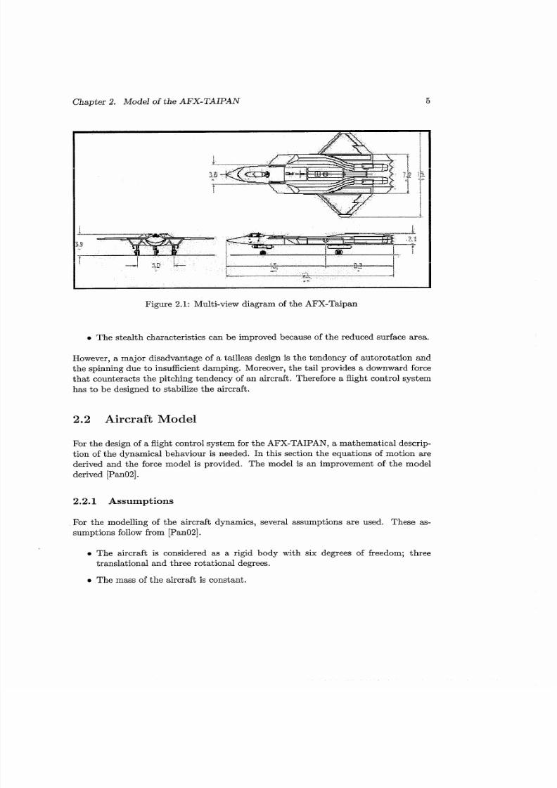
a tailless design. The aircraft is depicted in Figure 2.1. The full specification of the
aircraft is given in [GPT99].
The aircraft is equipped with two JSF119-611 Afterburning Turbofans. These engines
enable the use of a 3D thrust vectoring system in order to improve the manoeuvrability
of the aircraft. The maximum pitch and yaw angle of the nozzles are fixed to 20°.Moreover, the control system of the aircraft contains outboard split ailerons. The
application of thrust vectoring allowed the designers to consider a tailless design. The
main adva ~tag esf a tailless configuration are:
o By removing the tail and shorteniag of the fnselage, the drag of the aircraft c m
be reduced by 20% - 35%.
The structural weight of the aircraft can be reduced with 10%
0 The range for a given fuel load can be increase because of the reduced drag.
7/28/2019 Control Bien Explicado de Un Avionn
http://slidepdf.com/reader/full/control-bien-explicado-de-un-avionn 9/51
Chapter 2. Model of the AFX-TAIPAN 5
IFigure 2.1: Multi-view diagram of the AFX-Taipan
0 The stealth characteristics can be improved because of the reduced surface area.
However, a major disadvantage of a tailless design is the tendency of autorotation and
the spinning due to insufficient damping. Moreover, the ta il provides a downward force
that counteracts the pitching tendency of an aircraft. Therefore a flight control system
has to be designed to stabilize the aircraft.
2 .2 Aircraft Model
For the design of a flight control system for the AFX-TAIPAN, a mathematical descrip-
tion of the dynamical behaviour is needed. In this section the equations of motion are
derived and the force model is provided. The model is an improvement of the model
derived [Pan02].
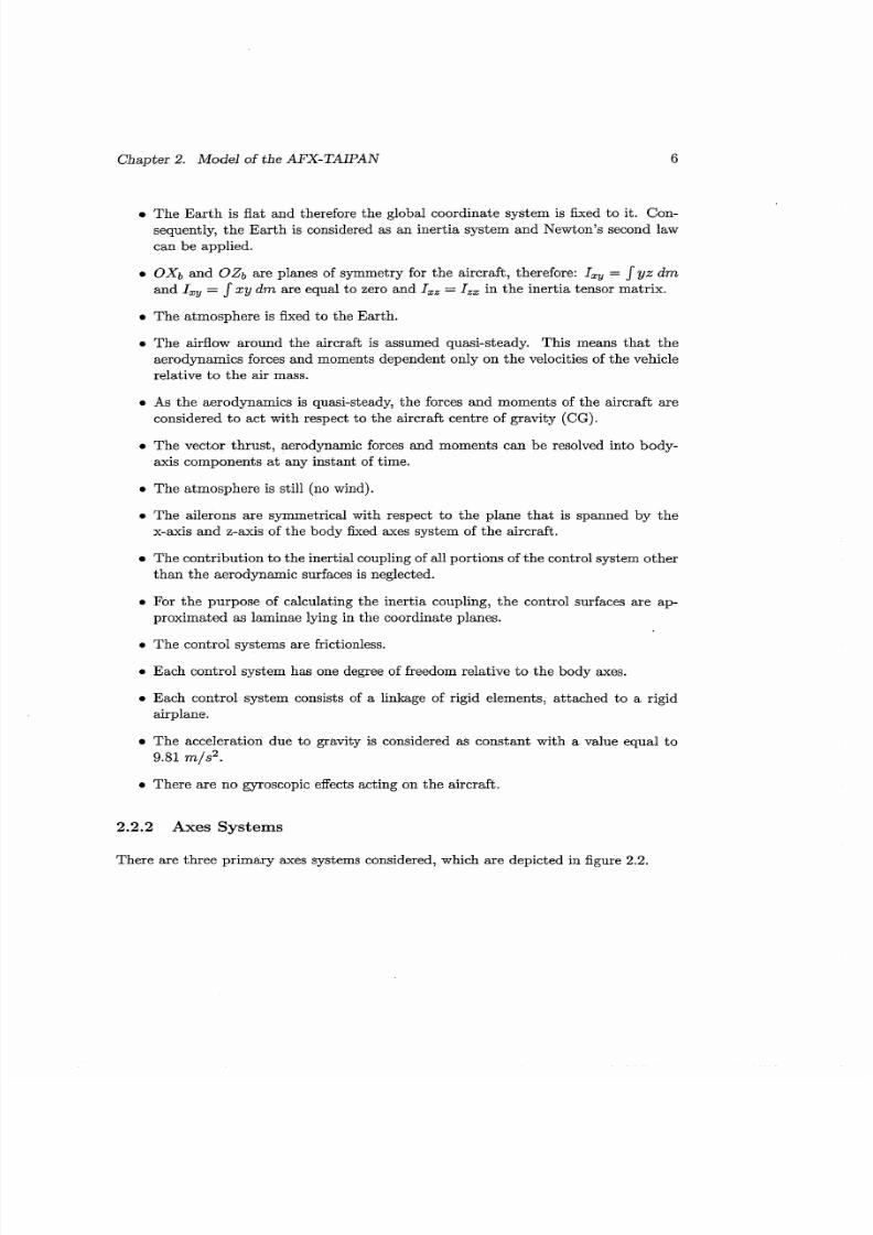
2.2.1 Assumptions
For the modelling of the aircraft dynamics, several assumptions are used. These as-
sumptions follow from [Pan02].
0 The aircraft is considered as a rigid body with six degrees of freedom; three
translational and three rotational degrees.
0 The mass of the aircraft is constant.
7/28/2019 Control Bien Explicado de Un Avionn
http://slidepdf.com/reader/full/control-bien-explicado-de-un-avionn 10/51
Chapter 2. Model of the AFX-TAIPAN 6
The Earth is flat and therefore the global coordinate system is fixed to it. Con-
sequently, the Earth is considered as an inertia system and Newton's second law
can be applied.
0 O X b and OZb are planes of symmetry for the aircraft, therefore: Ix y= J yz dm
and Ixy= xy dm are equal to zero and I,, = I,, in the inertia tensor matrix.
0 The atmosphere is iixed to the Earth.
0 The airflow around the aircraft is assumed quasi-steady. This means that the
aerodynamics forces and moments dependent only on the velocities of the vehicle
relative to the air mass.
0 As the aerodynamics is quasi-steady, the forces and moments of the aircraft are
considered to act with respect to the aircraft centre of gravity (CG).
0 The vector thrust, aerodynamic forces and moments can be resolved into body-
axis components a t any instant of time.
0 The atmosphere is still (no wind).
0 The ailerons are symmetrical with respect to the plane that is spanned by the
x-axis and z-axis of the body fixed axes system of the aircraft.
The contribution to the inertial coupling of all portions of the control system other
than the aerodynamic surfaces is neglected.
0 For the purpose of calculating the inertia coupling, the control surfaces are ap-
proximated as laminae lying in the coordinate planes.
0 The control systems are frictionless.
0 Each control system has one degree of freedom relative to the body axes.
0 Each control system consists of a linkage of rigid elements, attached to a rigid
airplane.
The acceleration due to gravity is considered as constant with a value equal to
9.81 m/s2.
0 There are no gyroscopic effects acting on the aircraft.
2.2.2 Axes Systems
There are three primary axes systems considered, which are depicted in figure 2.2.

7/28/2019 Control Bien Explicado de Un Avionn
http://slidepdf.com/reader/full/control-bien-explicado-de-un-avionn 11/51
Chapter 2. Model of the AFX-TAIPAN
Figure 2.2: Aircraft axes systems
1. The first axes system is the Earth initial axes system(F).ecause2;s pointedtowards the North, 2;owards the East and 2; ownward, this reference frame
is also known as the NED axes system. The inerial frame is required for the
application of Newton's laws.
2. The second axes system is the aircraft-carried inertial axes system (z).his
axis system is obtained if the Earth inertial axes frame is translated to the center
of gravity of the aircraft with a vector
3. The body axes system (zb)s also an aircraft-carried axes system, with 2;
pointed towards the nose of the aircraft, 2; owards the right wing and 2;to the bottom of the aircraft. The axis system is obtained through successive
rotations of the aircraft-carried inertial frame with Tait-Bryant angles $ 8 and
6. The velocity vectors along these axes are u, v and w and the angular velocity
vectors are respectively: roll rate q, pitch rate q and yaw rate r. These velocity
vectors are sho-WIIin Egiire 2 .3

7/28/2019 Control Bien Explicado de Un Avionn
http://slidepdf.com/reader/full/control-bien-explicado-de-un-avionn 12/51
Chapter 2. Model of the AFX-TAIPAN
Figure 2.3: Body axes frame and velocities
2.2.3 State , input and output variables
The motion of an aircraft considered as a rigid body can be described by a set of six
coupled nonlinear second order differential equations. In general the model can bedescribed as
where g E Rn is the state vector, 2 E Rm is the input vector and - E R' s the output
vector.
The elements of the state and output vector are described in table 2.1, while the elements
of the input vector are shown in table 2.2. The translational velocities, u, v and w are
selected instead of the to tal velocity, &, the angle of attack, a, and the sideslip angle,
p, which are chosen in [Pan02]. The relation between the velocities of the aircraft with
respect to the inertia axis frame can be expressed in terms of th e velocities with respect

7/28/2019 Control Bien Explicado de Un Avionn
http://slidepdf.com/reader/full/control-bien-explicado-de-un-avionn 13/51
Chapter 2. Model of the AFX-TAIPAN
Table 2.1: State definitions
I w I z component of velocity in body axes I m / s IP I Roll rate in body axes I r a d l sa I Pitch rate in bodv axes I r a d l s
Unit
mls
m / s
St&,es
u
v
Ix I x ~ositionf CG in inertial frame m
Defi~iticr,
x component of velocity in body axes
v component of velocity in body axes
Yz
1 I Yaw ande
-40
Table 2.2: Input Definitions
y position of CG in inertial frame
z ~ositionf CG in inertial frame
Unit
Thrust force engine 1
m
m
Roll angle
Pitch angle
y,~ I Yaw angle of nozzle 1 I r a d
T? I Thrust force enaine 2 1 N
r a d
r a d
- - Ipn2 Pitch angle of nozzle 2 r a d
vnz Yaw of nozzle 2 , r a d ,
7/28/2019 Control Bien Explicado de Un Avionn
http://slidepdf.com/reader/full/control-bien-explicado-de-un-avionn 14/51
Chapter 2. Model of the AFX-TAIPAN
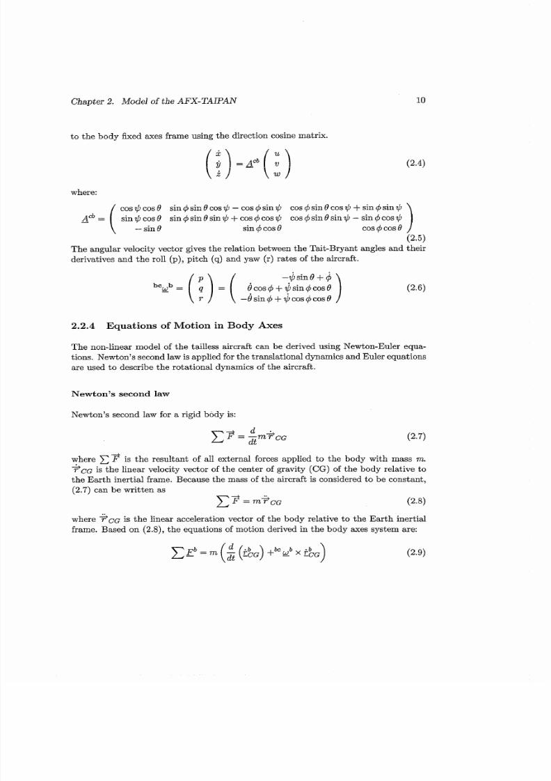
to the body fixed axes frame using the direction cosine matrix.
where:
cos$ cos 8 sin q5sin 8 cos$ - cos4 sin$ cos4 sin 8 cos$ + sin q5 sin .JI
sin$cosO sinq5sin8sin$+cosq5cos$ cos~sin8sin$-sinq5cos?l,- ( - in B sin 4 cos 13 cos q5cos 8
(2.5)The angular velocity vector gives the relation between the Tait-Bryant angles and their
deri-mtiws 2nd the re!! Y nit&- ( n )Y / a d aw (r) rates of the aircraft.
2.2.4 Equations of Motion in Body Axes
The non-linear model of the tailless aircraft can be derived using Newton-Euler equa-
tions. Newton's second law is applied for the translational dynamics and Euler equationsare used to describe the rotational dynamics of the aircraft.
Newton's second law
Newton's second law for a rigid body is:
where C2 s the resultant of all external forces applied to the body with mass rn.
is the linear velocity vector of the center of gravity (CG) of the body relative to
the Earth inertial frame. Because the mass of the aircraft is considered to be constant,(2.7) can be written as
where ?cG is the linear acceleration vector of the body relative to the Ear th inertial
fxm e. Based on (2.8)' the eq ~at fon sf motion derived in the body mes system are:

7/28/2019 Control Bien Explicado de Un Avionn
http://slidepdf.com/reader/full/control-bien-explicado-de-un-avionn 15/51
Chapter 2. Model of the AFX-TAIPAN
with
where (2.6)is the angular velocity vector of the aircraft with respect to the body
fixed frame. This results in the following force equations
CF!= m(iL+qw-rli)
CF; m(ir+ru-pw)
nL@' m(w+pv-qu)
Euler Equations
Euler equations are applied for the rotational dynamics of the aircraft. The rotational
dynamics can be described as
g c o = 2co (2.12)
where C g C ~s the resultant of the external moments applied to a body relative toits center of gravity. is the angular momentum vector relative to the center of
gravity of th e aircraft, which can be described by
~ C GJ C G ~ (2.13)
where JCMs the inertia tensor of the rigid body. From (2.12) and (2.13),the rotational
equations of motion derived in the body axes system are:
Tnis results in the following equations.

7/28/2019 Control Bien Explicado de Un Avionn
http://slidepdf.com/reader/full/control-bien-explicado-de-un-avionn 16/51
Chapter 2. Model of the AFX-TAIPAN
2.2.5 Forces and Moments
The forces and moments a t the center of gravity of the aircraft have components due
to the ga-$Ita~ iona l ects, ~erodjrna+~csffect m d the f~rces ~ dcmezts due t c the
3d thrust vectoring system. The force model is based on the force model derived in
[Pan02].
Gravitational forces
The components of the gravitational forces in the aircraft center of gravity with respect
to the body axes are:
= -mg sin 6j
F : ~ = mg sin(+) cos(0)
F ; ~ = mg cos(+) cos(6)
Aerodynamic forces and moments
The aerodynamic forces acting on the aircraft are basically the drag, lift, side-force and
the aerodynamic rolling, pitching and yawing moment.
where 7j= & v , ~ s the dynamic pressure of th e free-stream, S the wing reference area, b
the wing span and mac the mean aerodynamic chord. The values of these parameters are
determined in [GPT99] and given in table A. l of Appendix A. CD, CL,Cy Cl,Cmand
Cn are the dimensionless coefficients of drag, lift, side-force, rolling-moment, pitching-
moine~t d yzwing-moment respectively. The aerodynamic coeEcier;ts tire mainly a
function of the angle of attack and the side-slip angle. Although the dependency of
the aerodynamic coefficients to these parameters can be very nonlinear in high Mach
number region, a linear approximation is used. The aerodynamic coefficients are derived

7/28/2019 Control Bien Explicado de Un Avionn
http://slidepdf.com/reader/full/control-bien-explicado-de-un-avionn 17/51
Chapter 2. Model of the AFX-TAIPAN
in [GPT99] and shown below.
The values for the aerodynamic parameters ci are given in table A.2. In (2.19) the
parameters Peg,aeq,,, and ueq are obtained from [Pan021 and are given in table A.3.
Since the drag force is defined in negative flight direction and the lift force perpendic-
ular to the flight direction pointed to the top of the aircraft, the components of these
aerodynamic forces in the body fixed frame are:
Thrust forces
The thrust forces are generated by a 3D thrust vectoring system. The thrust forces in
body axes frame are derived using goniometric relations
where TI and T2denote the magnitude of the thrust force, pnl and p,2 the pitch angle of
the rmzz!es a d nl &ridyn2 the yaw ar,gle of the nozzles. The moments on the aircraft
generated by the thrust forces are

7/28/2019 Control Bien Explicado de Un Avionn
http://slidepdf.com/reader/full/control-bien-explicado-de-un-avionn 18/51
Chapter 2. Model of the AFX-TAIPAN 14
where d is the distance between the nozzle exit center and the aircraft vertical plane
and XCg he distance from the nozzle exit to the aircraft center of gravity.
With this, the dynamical model of the aircraft is derived. The combination of the
equations of motion and the force model yields in six coupled nonlinear second order
differential equations. The model can be used for the determination of the response of
the aircraft.
7/28/2019 Control Bien Explicado de Un Avionn
http://slidepdf.com/reader/full/control-bien-explicado-de-un-avionn 19/51
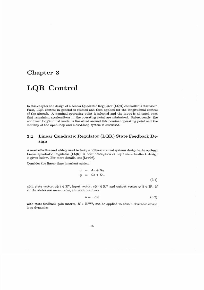
Chapter 3
LQR Control
In this chapter the design of a Linear Quadratic Regulator (LQR) controller is discussed.
First, LQR control in general is studied and then applied for the longitudinal control
of the aircraft. A nominal operating point is selected and the input is adjusted such
that remaining accelerations in the operating point are minimized. Subsequently, the
nonlinear longitudinal model is linearized around this nominal operating point and the
stability of the open-loop and closed-loop system is discussed.
3.1 Linear Quadratic Regulator (LQR) State Feedback De-
sign
A most effective and widely used technique of linear control systems design is the optimal
Linear Quadratic Regulator (LQR).A brief description of LQR state feedback design
is given below. For more details, see [Lew98].
Consider the linear time invariant system
with state vector, x(t) E Rn, input vector, u(t) E IRm and output vector y(t) E Rz. If
all the states are measurable, the state feedback
with sta te feedback gain matr ix, K E BmZn, an be applied to obtain desirable closed
loop dynamics

7/28/2019 Control Bien Explicado de Un Avionn
http://slidepdf.com/reader/full/control-bien-explicado-de-un-avionn 20/51
Chapter 3. LQR Control
x = (A - BK)x- A&
For LQR control the following cost function is defined:
Substitution of (3.2) into (3.4) yields:
The objective of LQR control, is to find a state feedback gain matrix, K , such that
the cost function (3.5) is minimized. In (3.5), the matrices Q E RnXnand R E Rmxm
are weighting matrices, which determine the closed-loop response of the system. The
matrix Q is a weighting matrix for the states and matrix R is a weighting matrix for the
input signals. By the choice of Q and R a consideration between response time of the
system and control effort can be made. Q should be selected to be positive semi-definite
and R to be positive definite.
To minimize the cost function, (3.5) should be finite. Since (3.5) is an infinite integral,
convergence implies x(t) + 0 and u(t)+ 0 as t -+w. This in turn guarantees stability
of the closed-loop system (3.3). To find the optimal feedback, K , i t is assumed tha t
there exists a constant matrix P such that:
Substituting (3.6) into (3.5) results in
If the closed-loop system is stable, x( t) -+ 0 for t + w. Now, J is a constant that
depends only on the matrix P and the initiai conditions. ~t this point, it is possibie
to find a state feedback, K , such that the assumption of a constant matrix P holds.
Substituting the differentiated form of (3.6) into (3.3) yields:

7/28/2019 Control Bien Explicado de Un Avionn
http://slidepdf.com/reader/full/control-bien-explicado-de-un-avionn 21/51
Chapter 3. LQR Control
and therefore
A ; P + P A ~ + Q + K ~ R K = O
Substitution of (3.3) into (3.9) yields
the following result can be obtained.
This result is the Algebraic Riccati Equation (ARE). It is a matrix quadratic equation,
which can be solved for P given A,B,Q and R, provided that (A,B) is controllable and
(Q4 ,A ) is observable. In th at case (3.12) has two solutions. There is one positive definite
and one negative definite solution. The positive definite solution has to be selected.
Summarizing, the procedure to find the LQR state feedback gain matrix K is:
Select the weighting matrices Q and R
Solve (3.12) to find P.
Compute K using (3.11).
With this, the optimal feedback u = -R-lBTPx is obtained.
3.2 Longitudinal LQR-Control application
The above LQR-theory is applied for the longitudinal flight control of the tailless air-
craft. First the longitudinal dynamics are formulated and a nominal operating point is
selected. The nonlinear model is linearized around this operating point and an LQR
controller is designed.

7/28/2019 Control Bien Explicado de Un Avionn
http://slidepdf.com/reader/full/control-bien-explicado-de-un-avionn 22/51
Chapter 3. LQR Control
3.2.1 Longitudinal dynamics
The full model of the tailless aircraft is described in Chapter 2. In this chapter only the
iongitudinai dynamics are v~ua I--~ ~ ~ ~ b ~ d i ~ r d:A-- ' mode! of t h e AFX-TAIPAX ir,
body axes are defined as
& = fion k&-m ~zopz) (3.13)
Y = glon(Z~m, (3.14)
where gz, E IR4 = [8 u w q]T is the state vector, uz, E R2 = [T, pniIT is the
input vector and y E R4 = [8 u w q]T is the output vector. It should be noted
that for the longitudinal model, there are three degree of freedom and two independentinputs. The longitudinal dynamics are considered for a side velocity v = 0, roll angle
4 = 8 a ym - sngk $ = O. The mgz!ar dcxit ies p ESK!r ere dsc! eqm! t o zero.
The thrust force and pitch angle of both engines are assumed to be equal and the yaw
angle for the nozzle is considered to be zero. The dynamic equations, flon (a,,,,)are defined as follows:
m - q w
1+- (2Ti cos (pni)-mg sin (8))m - q w
1- C L ~- LI (arctan (E) a,,) - pc~zq
ZfHSti) =-
+ q u(1+ $)+
~ f g ~CDO+cm (arctan ( f )- aeq)+ :-m +qu
(1+$)1
+-m + qu
(2Ti sin (pni)+mg cos (8))
1+- (2% sin (pni)Xq)
I5rY

7/28/2019 Control Bien Explicado de Un Avionn
http://slidepdf.com/reader/full/control-bien-explicado-de-un-avionn 23/51
Chapter 3. LQR Control
Table 3.1: Equilibrium states and remaining accelerations
The vdues of the parameters can be found in table A .2 and table A.3 of Appendix A.
3.2.2 Operating point
In order to design a LQR controller, the nonlinear model (3 .15) has to be linearized
around a certain equilibrium point. :p:n is an equilibrium point of (3 .13) if there exists
ueq such tha t fi,(gpQ,, &) = 0 .-1 on
Because it is not possible to find an equilibrium analytically, nonlinear optimization
techniques are used to find values for the elements of the inputs Ti and pni such that
the sum of the squared remaining acceleration is minimized for a given operating point.
The objective function 0 is:
The upper and lower bound for the optimization parameters are:
20-- 20
180T ad < pni 5 -T ra d
180
The next thing to do is to determine an initial operating point. For the initial operating
point it is desired that this is an equilibrium point. From (3 .13) it can only be concluded
that the pitch velocity, q, has to be equal to zero. Further, the inputs Ti nd p,i
are kept at a fixed value of respectively 50.000 N and 0 rad. The remaining states
u, w and 0 are used as optimization parameters to minimize the sum of the scpared
accelerations on the aircraft (3 .16) . The results are listed in table 3.1. This operating
point is considered as the nominal operating point. It can be observed that the maximal
remaining acceleration is -3.3358 rad / s2 . This means that no equilibrium point
is found.
7/28/2019 Control Bien Explicado de Un Avionn
http://slidepdf.com/reader/full/control-bien-explicado-de-un-avionn 24/51
Chapter 3. LQR Control
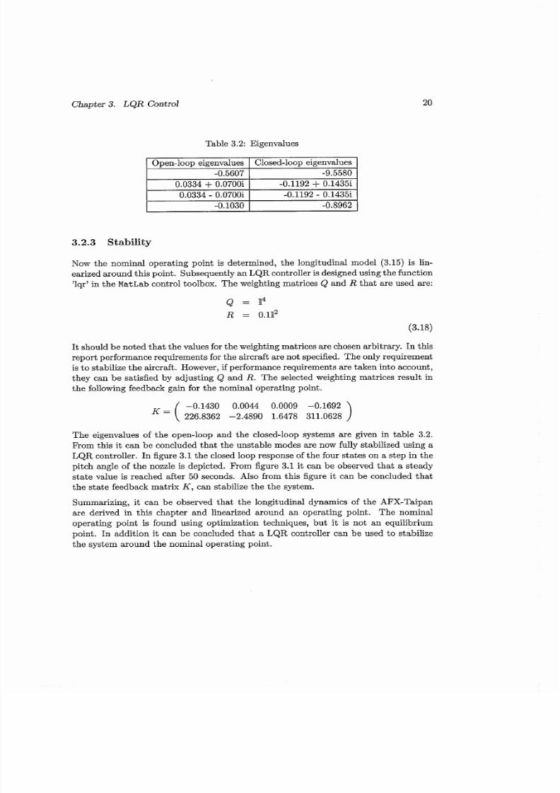
Table 3.2: Eigenvalues
I Open-loop eigenvalues I Closed-loop eigenvalues1 0.5607 1 -9.5580 1
3.2.3 Stability
NGWhe n~mina ! perzting poht is determined, the !ongitudind mnde! I-?----5) is 1 i ~ -
earized around this point. Subsequently an LQR controller is designed using the function
'lqr' in the MatLab control toolbox. The weighting matrices Q and R that are used are:
It should be noted tha t the values for the weighting matrices are chosen arbitrary. In this
report performance requirements for the aircraft are not specified. The only requirement
is to stabilize the aircraft. However, if performance requirements are taken into account,
they can be satisfied by adjusting Q and R. The selected weighting matrices result in
the following feedback gain for the nominal operating point.
The eigenvalues of the open-loop and the closed-loop systems are given in table 3.2.
From this it can be concluded that the unstable modes are now fully stabilized using a
LQR controller. In figure 3.1 the closed loop response of the four states on a step in the
pitch angle of the nozzle is depicted. From figure 3.1 it can be observed that a steady
state value is reached after 50 seconds. Also from this figure it can be concluded tha t
the s tate feedback matrix K , can stabilize the the system.
Summarizing, it can be observed that the longitudinal dynamics of the AFX-Taipan
are derived in this chapter and linearized around an operating point. The nominal
operating point is found using optimization techniques, but it is not an equilibrium
pifit. In addition it, can be concluded that a LQR controller can be used to stabilize
the system around the nominal operating point.

7/28/2019 Control Bien Explicado de Un Avionn
http://slidepdf.com/reader/full/control-bien-explicado-de-un-avionn 25/51
Chapter 3. LQR Control
lo-5 Step Response
time time
time time
Figure 3.1: Response to a step change in command pitch angle of the nozzle

7/28/2019 Control Bien Explicado de Un Avionn
http://slidepdf.com/reader/full/control-bien-explicado-de-un-avionn 26/51
Chapter 4
Gain Scheduling
The subject of this chapter is gain-scheduling. First, gain-scheduling is discussed in
general. An approach is developed to construct automatically a regular grid of operating
points. This approach is based on [AkmOl] and uses the concept of the stability radius.
4.1 Introduction
Gain-scheduling is the main technique that is used in flight control systems. It is acontrol method t ha t can be applied to linear time-varying and nonlinear systems. The
difference between classical control techniques and gain-scheduled control, is that a gain-
scheduled controller can provide control over an entire flight envelope, while a classical
controller is only valid in the neighbourhood of a single operating point. Many different
controller strategies, for example precompensation of a nonlinear gain with the inverse
gain function, can be viewed as gain scheduling. However, in this report gain scheduling
will be considered as the continuously variation of the controller coefficients according
to the current value of the scheduling signals.
According to [RSOO]the design of a gain scheduled controller for a nonlinear plant can
be described with a four step procedure.
The first step involves the computation of a linear parameter varying model for
the plant. The most common approach is to linearize the nonlinear plant around
a selection of equilibrium points. This results in a family of operating points.
The second step is to design a family of controllers for the linearized models in
each operating poi&. B e c a ~ s ef the !inearizz;ticn, simple Bnear ccr,trc!!er design
methods can be used to stabilize the system around the operating point.
The th ird step is the actual gain scheduling. Gain scheduling involves the imple-
mentation of the family of linear controllers such tha t the controller coefficients
are scheduled according to the current value of the scheduling variables.
7/28/2019 Control Bien Explicado de Un Avionn
http://slidepdf.com/reader/full/control-bien-explicado-de-un-avionn 27/51
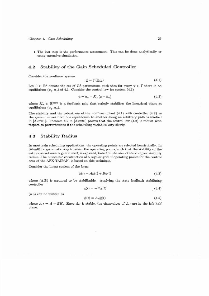
Chapter 4. Gain Scheduling 23
The last step is the performance assessment. This can be done analytically or
using extensive simulation.
4.2 Stability of the Gain Scheduled Controller
Consider the nonlinear system
ii= f (:,Id
Let I' c Rq denote the set of GS-parameters, such that for every y E I? there is an
equilibrium (x7, u7) of 4.1. Consider the control law for system (4.1)
where Ky E Rmxn is a feedback gain that strictly stabilizes the linearized plant at
equilibrium (g7, 7).
The stability and the robustness of the nonlinear plant (4.1) with controller (4.2) as
the system moves from one equilibrium to another along an arbitrary path is studied
in [AkmOl] Theorem 4.2 in [AkmOl] proves th at the control law (4.2) is robust with
respect to perturbations if the scheduling variables vary slowly.
4.3 Stability Radius
In most gain scheduling applications, the operating points are selected heuristically. In
[AkmOl] a systematic way to select the operating points, such th at the stability of the
entire control area is guaranteed, is explored, based on the idea of the complex stability
radius. The automatic construction of a regular grid of operating points for the control
area of the AFX-TAIPAN, is based on this technique.
Consider the linear system of the form:
where (A,B) is assumed to be stabilisable. Applying the state feedback stabilizing
controller
u(t) = -Kg(t) (4.4)
(4.3) can be written as
~ ( t )Ad:(t) (4.5)
where ACl= A - BK. Since Ad is stable, the eigenvalues of Ad are in the left half
plane.
7/28/2019 Control Bien Explicado de Un Avionn
http://slidepdf.com/reader/full/control-bien-explicado-de-un-avionn 28/51
Chapter 4. Gain Scheduling 24
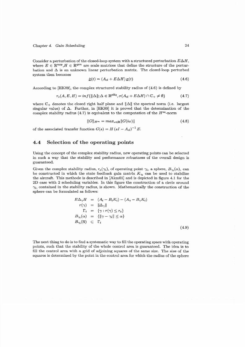
Consider a perturbation of the closed-loop system with a structured perturbation E A H ,
where E E WnxP,H E Rqxn are scale matrices tha t define the structure of the pertur-
bation and A is an unknown linear perturbation matrix. The closed-loop perturbed
system then becomes
k ( t )= (Ad +EAH) :(t) (4.6)
According to [EK89], the compkx structnred stability r a d i~ sf (4.6) is defi~e d y
rc(A,E, H ) = inf 1 1 All; A E Wpxq, a(Ad f EAH) nC+# 0)
where C+ denotes the closed right half plane and IlAll the spectral norm (i.e. largest
singular value) of A. Further, in [HK89] it is proved that the determination of the
complex stability radius (4.7) is equivalent to the computation of the Hco-norm
of the associated transfer function G(s) = H (sI-A&)-' E.
4.4 Selection of the operating points
Using the concept of the complex stability radius, new operating points can be selected
in such a way that the stability and performance robustness of the overall design is
guaranteed.
Given the complex stability radius, r,(yi), of operating point yi, sphere, Byi (a) , can
be constructed in which the state feedback gain matrix Kyi can be used to stabilize
the aircraft. This methode is described in [AkmOl] and is depicted in figure 4.1 for the
2D case with 2 scheduling variables. In this figure the construction of a circle around
yi, contained in the stability radius, is shown. Mathematically the construction of the
sphere can be formulated as follows:
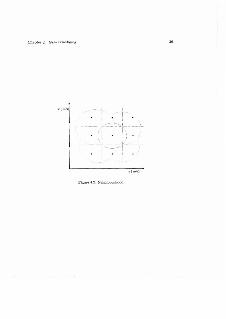
The next thing t o do is to find a systematic way to fill the operating space with operating
points, such that the stability of the whole control area is guaranteed. The idea is to
fill the control area with a grid of adjoining squares of the same size. The size of the
squares is determined by the point in the control area for which the radius of the sphere

7/28/2019 Control Bien Explicado de Un Avionn
http://slidepdf.com/reader/full/control-bien-explicado-de-un-avionn 29/51
Chapter 4. Gain Scheduling
Figure 4.1: Construction of By,i(a)
in which the system can be stabilized is the smallest. The centers of the squares are the
new operating points. This approach is depicted in figure4.2. With this, the procedure
to construct a regular grid of operating points is completed.
7/28/2019 Control Bien Explicado de Un Avionn
http://slidepdf.com/reader/full/control-bien-explicado-de-un-avionn 30/51
Chapter 4. Gain Scheduling
u [ m/sl
Figure 4.2: Neighbourhood
7/28/2019 Control Bien Explicado de Un Avionn
http://slidepdf.com/reader/full/control-bien-explicado-de-un-avionn 31/51
Chapter 5
Longitudinal Gain Scheduling
In this chapter the gain scheduling technique will be applied for the longitudinal control
of the AFX-TAIPAN. The longitudinal model is described in Chapter 3. A regular grid
of operating points is constructed according the technique of Chapter 4. For these
operating points LQR controllers are designed. The resulting global gain scheduled
controller is applied to the longitudinal flight control system of the AFX-TAIPAN. In
figure 5.1 a schematic representation of the design approach is depicted.
5.1 Scheduling Variables
The first step in the design approach is the selection of the scheduling variables. In
[AkmOl] it was proved that the scheduling variables should vary slowly to maintain
stability when the aircraft moves from one equilibrium point to another. From @ug91]
and [RSOO] it also follows that the scheduling variables should be slowly varying and
capture the nonlinearities of the system. However, this is only a qualitative result.
In this report the forward velocity, u, and the downward velocity, w, are chosen as
scheduling variables. Intuitively, these variables are slowly time varying and capture
the dynamic nonlinearities. However, not all nonlinearities are captured. To captureall nonlinearities, the density of the air and the pitch angle should also be considered.
In this report the pitch angle and the density of the air are kept on a £wed value, such
that the nonlinearities caused by these parameters not occur.
5.2 Selection of the Operating Points
The next step is the selection of the operating points as described in Section 4.4. The
nominal operating point was earlier determined in Section 3.2.2. The nominal values of

7/28/2019 Control Bien Explicado de Un Avionn
http://slidepdf.com/reader/full/control-bien-explicado-de-un-avionn 32/51
Chapter 5. Longitudinal Gain Scheduling Control
Selection of!
scheduling variables 1
i', II Selection of I' operating points I' 4-I I1I I
I/ LinearizationI
I LQR Controller
Design
+ I/ Scheduling 1
electionOperatingPoints
iInitial operatingpoint iSelection of thecontrol area I
/ Find Control Neighbourho odI * Input Opitrnization* Linearization* LQRControl Design* Stability Radius C omputation* Construction of Stability Ball
Construction grid of
operating points-Figure 5.1: S t e ~ ~ ~ r o a c hain Scheduling

7/28/2019 Control Bien Explicado de Un Avionn
http://slidepdf.com/reader/full/control-bien-explicado-de-un-avionn 33/51
Chapter 5. Longitudinal Gain Scheduling Control
the scheduling variables are
which corresponds to a total velocity of 166.59 m/s and an 4.4' angle of attack. These
values are chosen because the remaining accelerations are minimized for this combina-
tion of scheduling variables. The nominal operating point is considered to be in the
middle of the area for which the controller is developed. The ranges of the scheduling
variables for which the controller is developed are:
It should be noted t ha t this is only a very small area of the entire flight envelope of
the AFX-Taipan. However, the principle of the selection of the operating points can be
applied in the same way for the entire envelope.
For a regular grid of 25 points within this control area, the radius of the sphere is
determined, in which the state feedback of this point is able to stabilize the system. For
each of these 25 points the input is optimized to minimize the remaining accelerations
and the model is linearized around these equilibrium points. Subsequently the stability
radius is computed. For the computation of the stability radius the structure of the
perturbations matrices E and H has to be defined. Because there is no uncertainty
in the first equation of (3.15), 8 = q, and unstructured disturbance is assumed, the
perturbation matrices are:
0 0 0 0
The singular values of G(s) = H (sI- ~d)-' E are computed between radls
and i~h.racl /sor all the poil?ts. The stability radius Is the Inverse of the lzrgest
singular value. Now the stability radius is known, the radius of the sphere B%(Q)
can be constructed as was s h c t ~ I~ figwe 4.1. In eight directicns the value fe r a is
determined such that Byi(a) ri. his is illustrated for the nominal operating point
in figure 5.2.
The maximal values for a for each of the 25 points are depicted in figure 5.3. From this
figure it appears that a,i, = 0.002 for all the points in the entire control area. This
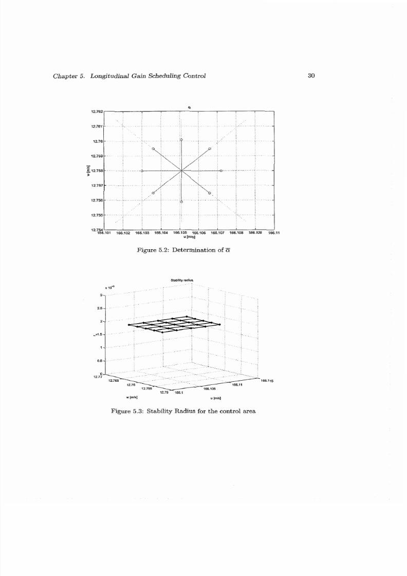
7/28/2019 Control Bien Explicado de Un Avionn
http://slidepdf.com/reader/full/control-bien-explicado-de-un-avionn 34/51
Chapter 5. Longitudinal Gain Scheduling Control
Figure 5.2: Determination of E
Figure 5.3: Stability Radius for the control area
7/28/2019 Control Bien Explicado de Un Avionn
http://slidepdf.com/reader/full/control-bien-explicado-de-un-avionn 35/51
Chapter 5 . Longitudinal Gain Scheduling Control
Operating Points
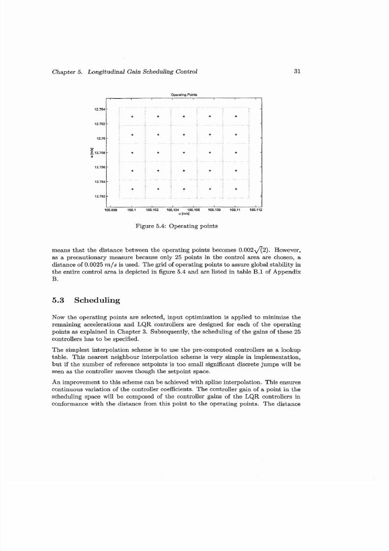
Figure 5.4: Operating points
means that the distance between the operating points becomes 0.002 d 2 ) . However,
as a precautionary measure because only 25 points in the control area are chosen, a
distance of 0.0025 mls is used. The grid of operating points to assure global stability in
the entire control area is depicted in figure 5.4 and are listed in table B. l of Appendix
B.
5.3 Scheduling
Now the operating points are selected, input optimization is applied to minimize the
remaining accelerations and LQR controllers are designed for each of the operating
points as explained in Chapter 3. Subsequently, the scheduling of the gains of these 25
controllers has to be specified.
The simplest interpolation scheme is to use the pre-computed controllers as a lookup
table. This nearest neighbour interpolation scheme is very simple in implementation,
but if the number of reference setpoints is too small significant discrete jumps will be
seen as the controller moves though the setpoiiit space.
An improvement to th is scheme can be achieved with spline interpolation. This ensures
continuous variation of the controller coefficients. The controller gain of a point i n the
scheduling space will be composed of the controller gains of the LQR controllers in
conformance with the distance from this point to the operating points. The distance

7/28/2019 Control Bien Explicado de Un Avionn
http://slidepdf.com/reader/full/control-bien-explicado-de-un-avionn 36/51
Chapter 5. Longitudinal Gain Scheduling Control
from the current point y o operating point i is calculated as follows:
The equilibrium input matrix and feedback gain matrix are computed using a percentage
of the U and K matrices according to the distance.
where
with q the number of operating points. Using (5.4) the resulting controller becomes:
5.4 Simulation
5.4.1 Flight path
In order to analyse the tracking capacities of the gain scheduled controller, a flight
path is defined. The flight path has to lie in the control area of figure 5.4. The initial
operating point is:
The first 100 seconds, it is desired to stay in this initial operating point. During the
next 100 seconds a step of 5 . m/s2 acceleration is applied in xb direction and a
step of -5. m/s2 n yb direction. After that the desired accelerations in xb and wbdirection are put to zero again. This means th at after 200 seconds the desired values
for u and w are constant again. It is desired to stay in tha t operating point for 100
seconds. This makes it possible to analyse the steady state response.
5.4.2 Simulation Results
Using the nonlinear longitudinal model of the AFX-TAIPAN and the gain scheduled
flight control system, simulations are executed. In figure 5.5 the desired and the actual

7/28/2019 Control Bien Explicado de Un Avionn
http://slidepdf.com/reader/full/control-bien-explicado-de-un-avionn 37/51
Chapter 5. Longitudinal Gain Scheduling Control
Actual and desired states
. . . .
- 3278 . . . . . . . . . . . . . . . . . . . . .U .mh'0
@ 0.3278 . . . . . . . . . . . .:.
. . . . . . . . . ..3278 . . . . . . .
time [s] time [s]
time [s] time [s]
Figure 5.5: Desired response and actual response
7/28/2019 Control Bien Explicado de Un Avionn
http://slidepdf.com/reader/full/control-bien-explicado-de-un-avionn 38/51
Chapter 5. Longitudinal Gain Scheduling Control
time [s] time [s]
L0 100 200 300
time [s]
-21 I0 100 200 300
time [s]
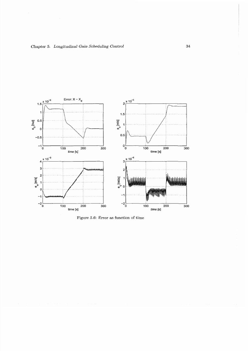
Figure 5.6: Error as function of time
7/28/2019 Control Bien Explicado de Un Avionn
http://slidepdf.com/reader/full/control-bien-explicado-de-un-avionn 39/51
Chapter 5 . Longitudinal Gain Scheduling Control 35
response are depicted during a 300 seconds simulation. From this figure it appears
that the desired trajectory and the actual trajectory do not agree. The error, which is
defined as the difference between the actual value of the states and the desired value of
the states, is depicted in figare 5.6. lt caE bbe observed that zi steady s tz te ermr rem&i.lns.
The reason for the steady state error is that the operating points which are used are
not equilibrium points. From table 3.1 it is shown that for the initial operating points
the acceleration of the aircraft is not equal to zero. Remaining accelerations for the
operating points are equivalent to a constant disturbance which acts on equilibrium
points. That is why a steady state error can be observed in figure 5.6. The error is
small enough such that the aircraft stays in the control area. This means tha t the gain
scheduled controller is able to stabilize the aircraft. However, if the desired trajectory
is chosen at the boundary of the control area, it could be possible that the remaining
accelerations take the aircraft out of the area for which the controller is deveioped. This
can lead to instability.
Summarizing, it can be concluded that the gain scheduled controller has been success-
fully applied to th e stabilization of the aircraft. However, a steady state error remains.

7/28/2019 Control Bien Explicado de Un Avionn
http://slidepdf.com/reader/full/control-bien-explicado-de-un-avionn 40/51
Chapter 6
6.1 Conclusions
0 In this report the six degree of freedom dynamical model of the AFX TAIPAN
is derived. Based on this six degree of freedom model, the longitudinal dynamics
are formulated.
In order to find an equilibrium point for the longitudinal dynamics of the aircraft,
optimization techniques are use to minimize the remaining accelerations. However,
it appeared that the remaining accelerations are non-zero. This means th at the
operating point found, is not a real equilibrium point.
0 LQR Control can be used to stabilize the AFX TAIPAN around an operating
point. The concept of the stability radius is used to determine the neighbourhood
of a n operating point in which the LQR controller is able to stabilize the nonlinear
system.
0 An approach to construct a regular grid of operating points for the gain scheduled
controller is provided to assure global stability of the entire control area. This ap-proach is based on the smallest control neighbourhood in a predetermined control
area.
0 The gain scheduled controller, based on 25 LQR controllers, is applied for the
lnngitudina! dyrmmic of the AFX-TAImN. The gain scheduled controller is able
to stabilize the aircraft. However, because the control area does not consist of a
link up of equilibrium points, a steady state error can be observed.
7/28/2019 Control Bien Explicado de Un Avionn
http://slidepdf.com/reader/full/control-bien-explicado-de-un-avionn 41/51
Chapter 6. Conclusions and Recommendations
6.2 Recommendations
0 In this report gain scheduling is applied for the longitudinal dynamics of the
AFX-TAIPAN. The scheduiing variables used are the forward and the downward
velocity of the aircraft. However, to capture all nonlinearities the pitch angle, 8 ,
and the density of the air, p , should also be considered. Moreover, gain scheduling
can be applied for the fuii order model.
The idea of gain scheduling is to move through the operating space along a p ath
of equilibrium points. However, the operating points which are found are not
equilibrium points. Additional control surfaces are needed to ensure that theoperating points become equilibrium points and that the gain scheduling theory
c= be applied.
0 The stability radius of the closed-loop system is very small. Since the stability
radius determines the number of operating points in the control area, the relation
between controller design and stability radius can be explored. After all, the
selection of the weighting matrices Q and R determines the state feedback gain
matrix, K, and the placement of the poles. By exploring the relation between the
controller design and the stability radius, the controller can be designed in such
a way that the stability radius is maximized.
The way to construct a regular grid as shown in Chapter 4, is based on the smallest
stability radius in the control area. If the stability radius changes a lot within thecontrol area this results in a large overlap of the stabilizing areas of the operating
point. More research can be done on minimize the overlap area.
0 In this report the performance requirements for the aircraft are not taken into
account. However, in general military standard requirements are specified. The
only requirement was to stabilize the system. Further research is required to find
a control design and an approach to select the operating points, such that the
performance requirements are satisfied.

7/28/2019 Control Bien Explicado de Un Avionn
http://slidepdf.com/reader/full/control-bien-explicado-de-un-avionn 42/51
Appendix A
Parameters of the AFX-Taipan
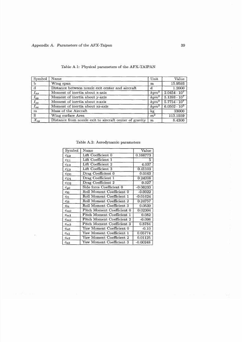
The physical parameters of the AFX-Taipan as derived in are listed in Table A.1. A full
description of th e aircraft is given in [GPT99]. In table A.2 the aerodynamic parameters
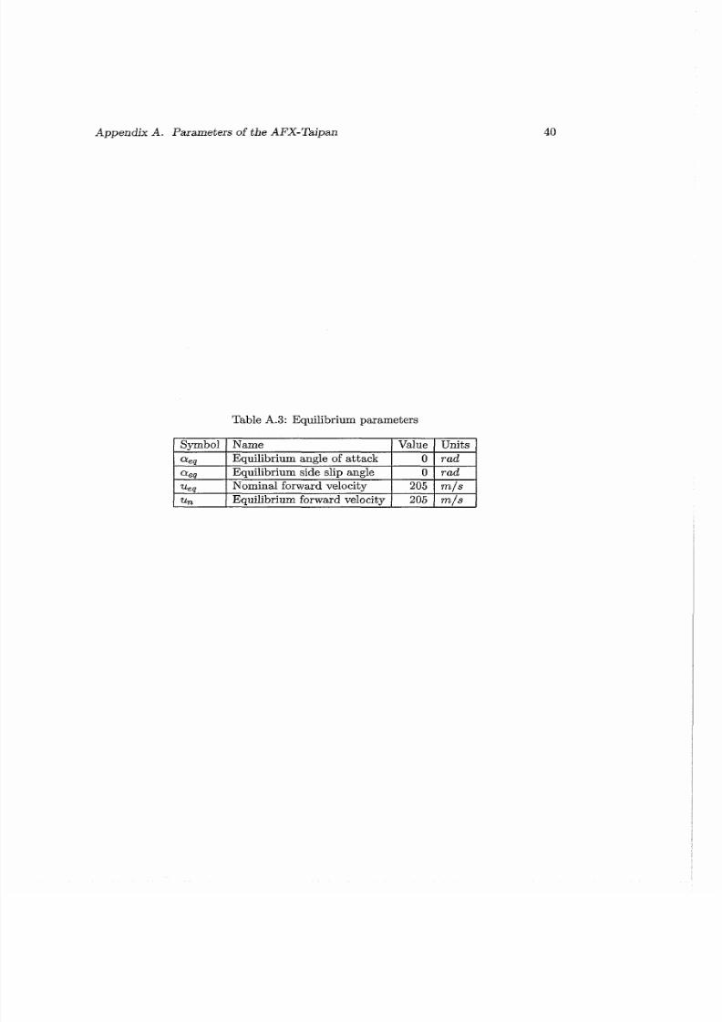
are listed as derived in [GPT99]. The equilibrium parameters for the aerodynamic
coefficients are depicted in A.3. These parameters follow from [Pan02].
7/28/2019 Control Bien Explicado de Un Avionn
http://slidepdf.com/reader/full/control-bien-explicado-de-un-avionn 43/51
Appendix A. Parameters of the AFX-Taipan
Table A . l : Physical parameters of the AFX-TAIPAN
I Svmbol 1 Name I Unit 1 Value 1I b"
I II Wina span I m 15.9593 1
Table A.2: Aerodynamic parameters
d
IXX
IVY
IZZ
I,,
m-X,,. Distance between nozzie exit center and aircraft
Moment of inertia about x-axis
Moment of inertia about y-axis
Moment of inertia about z-axis
Moment of inertia about xz-axis
d ' 1.2000 'kgm2
kgm2
kgm2
kom2
Mass of the Aircraft
Wing surface Area
Distance from nozzle exit to aircraft center of aravitv
Symbol 1 Name
2.0454. l o 7
5.1393 l o 7
5.7754 - l o7
6.0502 - l o 5
Value
-CL I
C L ~
- - I
C D ~ 1 Drag Coefficient 2 I 0.027 1
-kg
m"
m
cr.n 1 Lift Coefficient 0 1 0.166773
C L ~
~ D O
em
C yQ I Side force Coefficient 0 1 -0.06233
cm I Roll Moment Coefficient 0 I -0.0022
33000
113.1559
8.4300
Lift Coefficient 1
Lift Coefficient 2
"" I - - - - . - - -CI I Roll Moment Coefficient 1 1 -0.01624 1
5
4.037
Lift Coefficient 3
Drag Coefficient 0
Drag Coefficient 1
0.41103
0.0163
0.24208
"A
c 1 3
el4
%o
I IPitch Moment Coefficient 3 i 0.8784 1
%I I Pitch Moment Coefficient 1
L 7 I Pitch Moment Coefficient 2
) %o ] Yaw Moment Coefficient 0 1 -0.10 1en1 ) Yaw Moment Coefficient 1 i 0.05774 '~3 1 Yaw Moment Coefficient 2 1 0.01125
Roll Moment Coefficient 2
Roll Moment Coefficient 3
Pitch Moment Coefficient 0
0.082
-0.098
."- I I
%x I Yaw Moment Coefficient 3 1 -0.00248 1
0.24757
0.0539
0.02304
7/28/2019 Control Bien Explicado de Un Avionn
http://slidepdf.com/reader/full/control-bien-explicado-de-un-avionn 44/51
Appendix A. Parameters of the AFX-Taipan
Table A.3: Equilibrium parameters
Symbol
Qeq
Qen- zUeq
U n
Name
Equilibrium angle of attack
Equilibrium side slip angle
Value
0
0
m l s
m/s
- -Units
rad
radNominal forward velocity
Equilibrium forward velocity
205
205
7/28/2019 Control Bien Explicado de Un Avionn
http://slidepdf.com/reader/full/control-bien-explicado-de-un-avionn 45/51
Appendix B
Specification of the operating
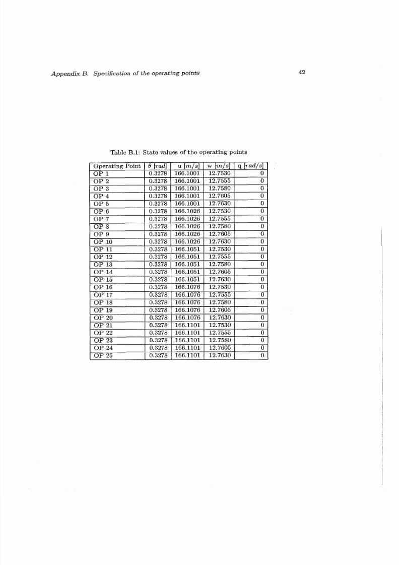
The operating points which are selected for the gain scheduled controller are listed in
table B.1. For these operating points the thrust force and the pitch angle of the nozzle
are optimized to minimize the largest remaining acceleration. The acceleration for each
operating point are given in table B.2.
7/28/2019 Control Bien Explicado de Un Avionn
http://slidepdf.com/reader/full/control-bien-explicado-de-un-avionn 46/51
Appendix B. Specification of the operating points
Table B.l: State values of the operating points
q [ rad l s ]
00
0
0
w [ m l s ]
12.753012.7555
12.7580
12.7605
Operating Point
OP 1OP 2
=I? 3
OP 4
0 [rad]
0.32780.3278
0.3278
0.3278
u [ m l s ]
166.1001166.1001
166.1001
166.1001

7/28/2019 Control Bien Explicado de Un Avionn
http://slidepdf.com/reader/full/control-bien-explicado-de-un-avionn 47/51
Appendix B. Specification of the operating points
Table B.2: Derivatives of th e states in the operating points
q rad/s2]
-0.0223-0.0144
w m/s2]
0.00050.0002
u m/s2]
-0.3438-0.1617
1 07 3
- Operating Point
OP 1OP 2
0 I 0.0198 1 0.0001 1 n nncF- V . V V V V I
8 [radls]
00

7/28/2019 Control Bien Explicado de Un Avionn
http://slidepdf.com/reader/full/control-bien-explicado-de-un-avionn 48/51
Appendix C
Matlab Files
This appendix contains a short description of the MATLAB iles which are used.
Model Derivation
parameters.m
The file parameters.m contains the parameters of th e aircraft as specified in
[PanO2].
Kinematics.mThe program Kinematics.m is used to formulate the kinematics of the 6th order
model of the AFX-Taipan. The file dir-cos-matrix is used for the computation of
the direction cosine matrix. The kinematics are saved in th e file Kinematics.mat.
F0rces.m
In th e file F0rces.m is used to formulate the force model of the AFX-Taipan. The
force model is saved in the file Forces.mat.
nonlinear6dof.m
In the file nonlinear6dof.m, the force model is substituted in the kinematics. This
results in the 6 dof dynamic model of the AFX-Taipan.
Aircraft1on.mThe program Aircraft-lon is used to compute the derivatives of the longitudinal
states as a function of the values of the states and inputs.
Linearization1on.m
The file Lictearizati:~ct~Im.ms used to compute the !inear !ongitudinal dynamics
of the AFX-Taipan.
matrixAlon.m and matrix-B-1on.m
The files matrix-A-1on.m and matrix-B-1on.m are used for the evaluation of the
A-matrix and B-matrix as function of the values of the states and inputs.

7/28/2019 Control Bien Explicado de Un Avionn
http://slidepdf.com/reader/full/control-bien-explicado-de-un-avionn 49/51
Append i x C. MATLABFiles
Initial Operating Point
1nitOP.m
The program Init0P.m is used for the computation of the initial operating point.
Optimization techniques are used to find the values of the states for which th e re-
maining accelerations of the aircraft are minimized, given the values of the input
signals. The file is used in combination with EqOP-lon.m, in which the opti-
mization is performed, objfOP-1on.m for the calculation of the objective function,
Aircraft_lon.m for the evaluation of the aircraft's dynamics and parameters.m.
Input Optimization
e Inpiii8piimizationlon.m
The program Input Optimization-lon.m is used to find the magnitude of the thrust
force and the pitch angle of the nozzle for which the remaining accelerations of
the aircraft are minimized, given the s tates of the aircraft. The file is used in com-
bination with EqIO-1on.m' in which the optimization is performed, objfI0-1on.m
for the calculation of the objective function, Aircrafi1on.m for the evaluation of
the aircraft's dynamics and parameters.m.
LQR Controller
LqrControl1erJon.m
In the file LqrController-1on.m the feedback gain matrix is computed using the
MATLABunction lqr. The file is used in combination with the files matrix-A-1on.m
and matrix-B-1on.m for the computation of the linear model. The stability of the
closed-loop system is evaluated using the file stability-1on.m.
Neighbourhood
Bal1Radius.m
The file Bal1Radius.m is used to compute the radius of the sphere around an
operating point for which the linear controller is able to stabilize the aircraft, as
explained in Chapter 4. The complex stability radius of the system is computed
with the program Stabi1ityRadius.m.
operatingpoints-1on.m
The file operatingpoints-1on.m is used to construct a regular grid of operating
points as expiained in Chapter 4. The distance between the operating points is
determined by the program Bal1Radius.m.

7/28/2019 Control Bien Explicado de Un Avionn
http://slidepdf.com/reader/full/control-bien-explicado-de-un-avionn 50/51
Appendix C. MATLAB iles
Gain-Scheduling
0 gs-cont rol1er.m
The file 9s-cantroller.%. is wed to compute the control input for a, raandom point
in the control area of the aircraft according to the distance to the individual
operating points. The LQR Controllers are saved in the file gs,con.mat.
0 gssim.md1
This program is a SIMULINKrogram which is used for the simulation of the
longitudinal model of the aircraft and the gain scheduled controller.
0 run-GSsim.mThe program run-GS-sim.m is used to set all parameters for the simulation of
the b~gitiididmde! of the &reraft m d the gain schedu!ed contro!!er. The file
p1otaircrajLlon.m is used for the visualization of the desired and actual respons
of the AFT-Taipan.

7/28/2019 Control Bien Explicado de Un Avionn
http://slidepdf.com/reader/full/control-bien-explicado-de-un-avionn 51/51
Bibliography
[AkmOl] Akmeliawati, R., Nonlinear Control for Automatic Flight Control Systems,University of Melbourne, PhD Thesis, 2001
[APHB02a] Akmeliawati,. R., Panella, I., Hill, R., Bil., C., Nonlinear Modeling and
Stabilization of a Tailless Fighter, RMIT University, 2002
[APHB02b] Akmeliawati,. R., Panella, I., Hill, R., Bil., C., Stabilization of a Tailless
[RSOO]
Fighter using Thrust Vectoring, RMIT University, 2002
Garth, J., Phillips, M., Turner J., AFX- Taipan, RMIT University, Under-
graduate Thesis in Bachelor of Engineering (Aerospace), 1999
Hinrichsen, D., Kelb, B., An Algoritm for the computation of the Structured
Complex Stability Radius, Automatica, Vol. 25, No 5 p. 771-775, 1989
Lewis, F.L., Linear Quadratic Regulator (LQR) State Feedback Design,
http://arri.uta.edu/acs/Lectures/lqr.pdf
Nelson, R.C., Flight Stability and Automatic Control, McGraw-Hill, 1989
Panella, I. Application of modern control theory to the stability and ma-
noeuvrability of a tailless fighter, RMIT University, Undergraduate Thesis in
Bachelor of Engineering (Aerospace), 2002
Rugh, W.J., Analytical Framework for Gain Scheduling, IEEE Control Sys-
tems Magazine, p. 79-84, January 1991
Rugh, W.J. , Shamma, J.S., Research on gain scheduling, Automatica, Vol.
36 , p. 1401-1425, 2000