Còpia de Benito_msthesis_FINAL2
99
PREDICTIVE MODELLING OF WETLAND HABITATS IN THE EBRO DELTA WITH A GIS APPROACH Xavier Benito Granell Màster en Planificació territorial: informació, eines i mètodes Facultat de Turisme i Geografia Universitat Rovira i Virgili IRTA – Unitat d’Ecosistemes Aquàtics
-
Upload
xavier-benito-granell -
Category
Documents
-
view
99 -
download
0
Transcript of Còpia de Benito_msthesis_FINAL2
PREDICTIVE MODELLING OF WETLAND HABITATS IN
THE EBRO DELTA WITH A GIS APPROACH
Xavier Benito Granell
Màster en Planificació territorial: informació, eines i mètodes
Facultat de Turisme i Geografia
Universitat Rovira i Virgili
IRTA – Unitat d’Ecosistemes Aquàtics
2
PREDICTIVE MODELLING OF WETLAND HABITATS IN THE EBRO DELTA
WITH A GIS APPROACH
Memòria del treball final del màster oficial de Planificació territorial: informació, eines i mètodes.
Per: Xavier Benito Granell
Dirigit per:
Dr. Carles Ibàñez Martí
Unitat d’Ecosistemes Aquàtics
IRTA – Sant Carles de la Ràpita
Dra. Rosa Trobajo Pujadas
Unitat d’Ecosistemes Aquàtics
IRTA – Sant Carles de la Ràpita
Dra. Yolanda Pérez Albert
Departament de Geografia
Universitat Rovira i Virgili
Vila-seca, Juliol de 2012

3
Agraïments
Aquest treball ha estat possible gràcies una beca predoctoral de la Universitat Rovira i Virgili
dins del conveni URV-IRTA. La base cartogràfica (Model digital d’elevació i ortofotomapes)
són propietat de l’Institut Cartogràfic de Catalunya (www.icc.cat).
4
Table of contents
Abstract ...................................................................................................................................... 5
1. Introduction ............................................................................................................................ 6
1.1 General context: deltaic system, wetland habitats and human colonization .................... 6
1.2 The aquatic habitats of the Ebro Delta ............................................................................. 7
1.3 Predictive habitat modelling ........................................................................................... 10
2. Hypotheses and objectives ................................................................................................... 15
3. Methods ................................................................................................................................ 17
3.1 Study area ....................................................................................................................... 17
3.2 Wetland habitats, terrain variables and hydrologic alterations ....................................... 19
3.3 Dependent variable: current distribution of wetland habitats ......................................... 20
3.4 The independent variables: elevation and distances to hydrologic boundaries .............. 33
3.5 Vegetation transects ........................................................................................................ 37
3.6 GIS development ............................................................................................................ 38
3.7 Statistical analysis ........................................................................................................... 45
3.8 Model implementation in the GIS .................................................................................. 47
4. Results and discussion .......................................................................................................... 48
4.1 Current distribution of wetland habitats in the Ebro Delta ............................................. 48
4.2 Logistic regression .......................................................................................................... 70
4.3 Probability of occurrence ................................................................................................ 85
5. General conclusions ............................................................................................................. 91
6. References ............................................................................................................................ 94
5
Abstract
Predictive habitat distribution models, derived by combining multivariate statistical methods
with Geographical Information System (GIS) techniques, have been recognised for their
utility in ecological modelling. The knowledge about potential distribution of natural habitats
requires the link between current presence or absence of biological communities and a set of
relevant environmental variables. This work examines the feasibility of using multiple logistic
regression to model wetland habitat distribution in the Ebro Delta and to analyse how the
riverine and marine influences affect its presence. Moreover, due to the high human
occupation in the Delta, their influence in terms of distances to hydrologic alteration was
assessed too. The predicted distribution was validated by comparison with a map of actual
habitat type distribution (CORINE land cover) and by field transects. The variables that best
explained the probability occurrence of habitats were soil elevation in habitats with higher
mean elevation (e.g. Cladium-type marshes, dunes/beaches, rice fields and riparian
vegetation) and distance to outer coast in habitats with lower elevations (coastal lagoons, tidal
flats, Salicornia-type marshes and reed beds). The influence of the road and channels on
habitats was reflected in higher soil elevations. The obtained prediction maps have provided
the first results on habitat modelling in the Ebro Delta. The restricted distribution of some
habitats due to human alteration may be the main reason of the mismatch between model
predictions and field data in some habitats.
6
1. Introduction
1.1 General context: deltaic system, wetland habitats and human colonization
The Ebro Delta (Catalonia, NE Iberian Peninsula) presents a formidable example of coastal
wetland with a high variability of ecological factors (topography, edaphology, hydrology and
climate) that play a key role in the configuration of its ecological gradients. The confluence of
of contrasted dynamics (i.e riverine, marine and underground) explains most of the Deltaic
variability across spatial and temporal scales. Due to human colonization (settlements,
agriculture, hunting, turism...) wetland habitats with high natural value have been displaced in
the periphery of the Delta where, significant remains of natural ecosystems subsist.
In natural habitats whose sustainability and multi-functional values are threatened, like deltas,
changes in land uses can have more environmental and ecological consequences than in other
ecosystem. Deltaic ecosystems of the Ebro River have particular ecological and economical
value because of their geographic position (interface between terrestrial and coastal zones)
and diversity of habitats (wetlands, coastal lagoons, bays...) (Ibàñez et al. 2010). Human
activities have led to a rapid deterioration of natural aquatic habitats since the beginning of
XX century, mainly, owing to rice cultivation. Until then, however, the dominant landscape
was determined by climatic, geomorphologic and biological factors, except areas transformed
to saltworks. Due to its natural evolution, the Ebro Delta underwent geomorphic changes such
as changes in river mouth and consequent erosion of abandoned lobes, filling of wetlands,
accretion and subsidence of the deltaic plain or regression and coastal progression (Curcó et
al. 1995). These natural processes led rapid modifications of the Delta’s configuration and in
its ecological condition. After several millennia of growth, Ebro Delta was under a river-
dominated dynamics but this trend changed a few decades ago in such a way that the present
Delta is now a wave-dominated coast (Jiménez and Sánchez-Arcilla 1993). This change is
mainly due to the construction of several dams along the river which has caused a nearly total
reduction (97%) of the solid river discharge (Rovira and Ibàñez 2007). Overall, the drastic
reduction of the sediment load slowed down the delta protrusion and intensified the delta
coastline washout (Mikhailova 2003).
7
The Ebro Delta contains some of the most important wetland areas in the western
Mediterranean. The majority of the Deltaic plain is devoted to rice agriculture and natural
areas cover only about 25% of the total surface. Among these areas, a set of natural habitats
are present: salt marshes, fresh-brackish marshes, coastal lagoons, sand dunes, natural springs
and bays. Moreover, most of these habitats are included and protected by several European
Directives (e.eg. Habitat Directive and Bird Directive) and regional laws (Ebro Delta Natural
Park). This ecological diversity coexists with a human population near 50.000 inhabitants,
which is located inside the Delta (15.000 inhabitants both Deltebre and Sant Jaume d’Enveja
villages) and along the inner border (approximately 35.000 inhabitants with Amposta and
Sant Carles de la Rapita villages). Urban zones, rice fields and other crops represents near
80% of total Delta surface. Intentisive human colonization in the Delta began at 1860’s with
the first marsh transformations to rice fields after the construction of irrigation channels
(southern hemidelta at 1860 and northern at 1912). From the beginning of 20th century until
present, human transformation of the Ebro Delta largely occurred through draining of
wetlands and the construction of an intensive irrigation system to bring fresh water from the
river to rice fields. According to several authors (Curcó 2006; Mañosa et al. 2001) natural
habitats declined its surface from 27.000 ha (80%) to 11.000 ha (30%) during the 1910-1960
period. The loss of natural habitats stopped during 1960s, but from 1970 to 1990 another 3000
ha of natural habitats were lost, leaving about 25% of total surface still occupied by lagoons
and marshes. Such habitat loss has produced a change in the vegetal and animal communities
present in the Delta. Present management in the Ebro Delta aims at maintaining a high
agricultural productivity and valuable bird populations in the natural areas which are included
in the Natural Park (Ibànez et al. 1997).
1.2 The aquatic habitats of the Ebro Delta
The ecological value of the Delta reflects a high biodiversity, being the aquatic ecosystems
the most important environments which support a representative sample of coastal wetlands.
The Ebro Delta shows 18 natural habitats listed in the annex 1 of the European Directive on
the conservation of natural habitats and of wild fauna and flora (Communities 1991). Bird and
fish populations represent the major faunal groups in order of importance together with
8
singularity of halophilous and psammophilous plant communities. There are several technical
reports (Curcó 2006) and scientific studies (Camp and Delgado 1987; Ibàñez et al. 1997;
Menéndez et al. 2002; Valdemoro et al. 2007) that attempt to describe the aquatic
environments of the Ebro Delta for achieving ecological information on their functioning.
These studies note that there is a combination of habitats along a gradient of riverine and
marine influence which confer wide environmental gradients. We consider the next main
habitat units that coexist in the Deltaic plain: estuary, rice fields, coastal lagoons, natural
wells, marshes, dunes and beaches, saltworks, bays and nearshore open sea domain.
Estuaries are dynamic ecosystems that form a transition zone between river environments and
ocean environments. Thus, estuaries are subjected to both marine influences (tides, influx of
saline water...) and river influences (flows, topography of bed...). The pattern of dilution
varies among systems. The Ebro Estuary is a salt-wedge estuary mainly dependent on the
river discharge since the tidal amplitude range is very low (Ibàñez et al. 1997). Ebro Estuary
extends from the mouth to 30 km approximately upstream, the position and presence of the
salt wedge being determined by the tidal range and river discharge.
The rice fields are the dominant landscape of the Delta and all aquatic ecosystems are
influenced by water coming from rice fields. The hydroperiod associated with rice production
is as follows: from April to December, a quantity of ca. 45 m3/s of river water is diverted to
the irrigation canals for continuous irrigation. The resulting eutrophication associated with
large amounts of fertilizer to enhance rice production, as well as pesticides, has led to a
decrease in biological diversity and negative effects on aquatic vegetation of lagoons (Comín
et al. 1991). Nevertheless, the rice fields form an aquatic matrix that link fluvial, lagoon and
marine environments through network channels of irrigation and drainage.
Coastal lagoons are littoral formations formed by the isolation of the marine domain through
the development of a sand bar which separates the water bodies from the open sea (Kjerfve
1994). For their position and origin, their hydrological regime is determined by sea water
inputs coupled with fresh water runoff from drainage of rice fields. For this reason, coastal
lagoons of Ebro Delta show a hydrologic pattern that is clearly reversed (i.e hypersaline
periods do not occur in summer as it would be expected in natural conditions). Aquatic
macrophyte assemblages of the coastal lagoons (e.g. Buda lagoons) have been modified due
9
to the creation of salinity gradient that allows the development of different environments with
the coexistence of several species of submerged macrophytes (Comín and Ferrer 1999).
Marshes are wetland areas between terrestrial and marine domains which are linked with the
coastal lagoons. Hydrological settings, mainly water and soil salinity, determine the presence
of fresh (Vilacoto area), brakish (Garxal) and salt marshes (Buda Island) in the Ebro Delta.
Vegetal communities of marshes are adapted to salinity content and soil moisture that
generally depends on frequency and duration of flooding events (Bouma et al. 2005). Marshes
play a key role exhibiting high primary productivity and assist important functions as nutrient
removal and sediment retention (Ibàñez et al. 2002). Under global warming scenario that have
produced eustatic sea level rise of 3.0 – 3,5 mmyr-1 over the past 15 years (IPCC 2001),
scientific literature pointed out the ecological importance of marshes which retain sediments
to offset sea level rise (Day et al. 2000).
The natural freshwater wells are systems of natural ponds situated along the inner Delta
border. In this area, underground water coming from often karstic inland areas (mainly
Montsia) overflows through the surface forming small water bodies no more than 7 metres
deep. A peat layer is present in this zone due to former palustral conditions, being catalogued
as a priority habitat *7210 Calcareous fens in Council Directive 92/43/EEC. These freshwater
wells are popularly called “ullals” and has been considerably altered by human activities,
mainly through draining to lower the underground water level (Capítulo et al. 1994). As a
result, Cladium marshes have been substituted by salt meadows dominated by Juncus genus in
the area of “ullals” de Panxa.
The shoreline of the Ebro Delta is occupied by sandy habitats that contain a very good
representation of dunes and beaches. These habitats also exercise a key role in balancing the
current coastline. The best dune systems of the Delta are placed in la Marquesa and el Fangar.
According to soil mobility, there is a zonation from embryonic dunes (Agropyro-Honckenyion
peploidis), shifting dunes with Ammophila arenaria and fixed dunes (Crucianellion
maritimae). The development of tidal flats with microbial mats in the inner coast of la Banya
peninsula represent another ecological value of these areas with particular hydrological
conditions due to their differential orientation of its coast. Thus, lower topographic levels and
NW dominant winds promote conditions to allow fluctuant moisture along drying and
flooding events.
10
The bays are coastal marine waterbodies partially closed with a constant connection to the
sea. In contrast to estuaries, the influence of freshwater is generally limited. In the Ebro Delta,
Fangar and Alfacs bays were originated through the confinement of water bodies due the
formation of spits parallel to the coast. The bays could be considered shallow coastal
ecosystems (2 m. mean depth for Fangar bay and 3,13 m. mean depth for Alfacs bay)(Llebot
et al. 2010), which involve marked spatial and temporal gradients.
The saltworks are traditional salt production areas, located in zones where salt marshes should
have their potential area. This artificial habitat is characterized by deep ponds with variable
salinity that contributes to the increasing diversity of Delta. The Trinitat saltworks were
included in the Natural Park since they provide favorable feeding habitats for the greater
flamingo Phoenicopterus ruber, an emblematic species of the Ebro Delta.
Nearshore open sea habitats are situated along the coastal area in front of the Ebro Delta. This
environment borders on the whole deltaic plain, and the set of beaches, bars and spits are
encompassed by it. A depth of 10 metres is considered the boundary between nearshore and
offshore open sea. Nearshore waters can differ substantially from offshore waters due to the
continental influence, and especially in an estuarine environment like delta. Thus, the latter
are more eutrophic, with higher nutrient and chlorophyll concentrations and different
phytoplankton composition (diatoms and dinoflagellates mainly).
The high diversity of habitats and processes present in the Ebro Delta offers a unique
opportunity to analyse the relationships between Ebro Delta habitats and their environment
and to infer their potential distribution in relation to riverine and marine influences
1.3 Predictive habitat modelling
The term “habitat” has been used in many ways in ecological studies. According to
Spelleberg, (1994) habitat can defined as “the locality or area used by a population of
organisms and the place where they live”. In ecology, the analysis of habitats-environment
relationship has always been a central issue. The major factor involved in habitat distribution,
especially in relation to plant communities, is climate in combination with geology or
hydrology. Habitat factors that are playing a key role in species distribution should be
11
considered since species ranges and richness are often correlated with these factors
(Vogiatzakis et al. 2006). The quantification of such relationships represents the core of
predictive geographical modelling in ecology. These models are generally based on various
hypotheses as to how environmental factors control the distribution of species and
communities (Guisan and Zimmermann 2000). Hence, models of habitat distribution are not
subjective models that predict how an area is suitable for development of a particular habitat
in relation to environment conditions.
The relationships between species, communtities or habitats (biotic entities) and
environmental variables are frequently studied using gradient analysis that underlie
hypotheses about species response functions (curves) to environmental gradients (Whittaker
1967). Austin and Smith (1989) defined three types of ecological gradients, namely indirect,
direct and resource gradients. Indirect gradients have no direct physiological influence on
species performance (slope, aspect, elevation, topographic position, geology). Direct gradients
are environment parameters that have physiological importance, but are not consumed (e.g
temperature, pH). Resource gradients address matter and energy consumed by plants or
animals (nutrients, water, light, food for plants, water for animals…). Generally, literature
pointed out that indirect variables usually replace a combination of different resources and
direct gradients in a sample way (Guisan et al. 1998; Guisan et al. 1999).
The real or actual vegetation is a patchwork of different classes or categories of communities.
Classifying these communities in accordance with some key allows one to construct a
vegetation map, which can be interpreted of actual vegetation that is normally more complex
than habitat units map. While they are a simplification of reality, habitat maps are important
data for correct environment management of a territory. The Ebro Delta has an important
environmental dataset of which habitat maps are included. This work derived from the
adaptation of the CORINE Biotopes project in Catalonia (Carreras and Diego 2007). But, this
kind of information (i.e habitat maps or vegetation maps) has a limited temporal variability.
Even in absence of human influence, vegetation dynamics is complex and intense, especially
in deltas which are subject to sharp environment gradients. In the Ebro Delta, the ecological
term of succession is applicable, defining the natural sequence in which a habitat replaces
another over the passage of time. Then, the potential vegetation is defined as the stable
community which would exist in an area as a consequence of progressive geobotanical
succession if man ceased to affect and alter the terrain. Curcó et al. (1995) made an exercise
12
to delineate potential vegetal domains based on topographical and sedimentological features
of the Deltaic plain. In this case, potential habitats will be more in balance with the salinity
and moisture conditions of the environment. A model that considers sites with their
disturbance features (e.g road or channels) might be expected to explain only a portion of the
variance in habitat type distribution. Even so, this approach can be a chance for applying in
the Delta.
The first step that has to be considered in predictive modeling is the link between habitat units
and mapped physical data. Several modelling methods have been used in scientific papers:
heuristic, decision trees and statistical methods. The last approach, mainly regression, is the
one most used to predict the value of the response variable if continuous, or the probability of
a variable if categorical (Vogiatzakis 2003). Most predictive modelling efforts has used
logistic regression to predict species (Rüger et al. 2005), vegetation assemblages (Davis and
Goetz 1990) or animal habitat (Corsi et al. 1999). A logistic regression is well-suited where
the dependent variable is dichotomous (presence/absence of habitats), and the technique
allows one predictor (binary logistic regression) or more than one (multiple logistic
regression). In addition the method lets a non-Gaussian distribution of the independent
variables (Hosmer and Lemeshow 2000). Also, the result of the regressions ranges from 0 to 1
so that is appropriate for the generation of a likelihood model (Álvarez-Arbesú and Felicísimo
2002). The application of this method to wetlands and aquatic ecosystems is not an exception.
(Narumalani et al. 1997) applied multiple logistic regression to predict aquatic macrophyte
distribution. Another similar study was applied to aquatic vegetation by van de Rijt (1996) for
predicting vegetation zonation in a former tidal area, while Shoutis et al. (2010) applied it for
predicting riparian vegetation based on terrain variables and different river orders. The final
step to consider in a predictive model is the model validation. Such evaluation consists in
determining the suitability of a model for specific applications. According to Pearce and
Ferrer (2000), wherever possible, evaluation is best undertaken with independent data
collected form sites other than those used to develop the model. If independent data are not
available, there are statistical techniques that fit the model in different degree, such as receiver
operating characteristic (ROC) plot methodology (for more details see methods section). The
next figure schematizes the generic steps of predictive modelling (Figure 1):
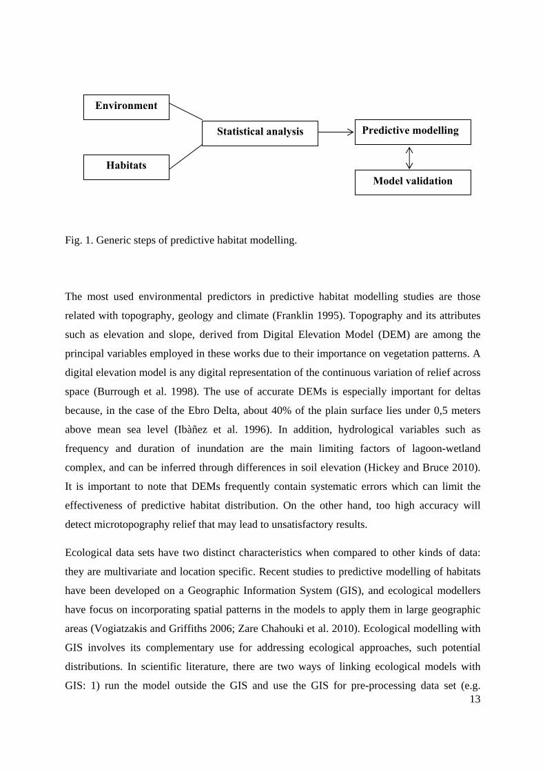
13
Fig. 1. Generic steps of predictive habitat modelling.
The most used environmental predictors in predictive habitat modelling studies are those
related with topography, geology and climate (Franklin 1995). Topography and its attributes
such as elevation and slope, derived from Digital Elevation Model (DEM) are among the
principal variables employed in these works due to their importance on vegetation patterns. A
digital elevation model is any digital representation of the continuous variation of relief across
space (Burrough et al. 1998). The use of accurate DEMs is especially important for deltas
because, in the case of the Ebro Delta, about 40% of the plain surface lies under 0,5 meters
above mean sea level (Ibàñez et al. 1996). In addition, hydrological variables such as
frequency and duration of inundation are the main limiting factors of lagoon-wetland
complex, and can be inferred through differences in soil elevation (Hickey and Bruce 2010).
It is important to note that DEMs frequently contain systematic errors which can limit the
effectiveness of predictive habitat distribution. On the other hand, too high accuracy will
detect microtopography relief that may lead to unsatisfactory results.
Ecological data sets have two distinct characteristics when compared to other kinds of data:
they are multivariate and location specific. Recent studies to predictive modelling of habitats
have been developed on a Geographic Information System (GIS), and ecological modellers
have focus on incorporating spatial patterns in the models to apply them in large geographic
areas (Vogiatzakis and Griffiths 2006; Zare Chahouki et al. 2010). Ecological modelling with
GIS involves its complementary use for addressing ecological approaches, such potential
distributions. In scientific literature, there are two ways of linking ecological models with
GIS: 1) run the model outside the GIS and use the GIS for pre-processing data set (e.g.
Statistical analysis Predictive modelling
Model validation
Environment
Habitats
14
coordinate system transformation, location of sample points…) and generate cartographic
outputs and 2) use GIS for extract metrics on environment mapped variables which will
conforms the core of statistical method and post-processing of the data through cartographic
display too (Felicísimo 2003; Felicísimo et al. 2002; Franklin et al. 2000). GIS-based spatial
analysis tools facilitate the representation of ecological data across the space and its
correlation with environmental data. In deltaic environment (among marshes, lagoons...),
surface elevation (or water depth) and inundation frequency are the most important
environment variables for vegetal zonation (Silvestri et al. 2005). Spatial analysis provides
tools for researchers to assess how these factors influence habitat type distribution, extract
metrics and explore the relationship between aquatic environments and topography by
investigating species zonation. For example, Hickey et al. (2010) examined the relationship
between distribution of salt marsh vegetation and the extent of tidal inundation using fine
elevation data; (Xie et al. 2011) defined several landscape units of freshwater wetlands in
Florida based on surface elevation; (Moran et al. 2008) linked spatial variation of flooding
regime with the vegetation zones in a karst wetland.
Habitats of the Ebro Delta are along environmental gradients which can be assessed to infer
distribution patterns. Getting a predictive model, one can establish a relation between the
habitat units and the environment data. The geographic scale of the Delta offers the
opportunity to incorporate Geographic Information System techniques for extrapolating over
a wide range those relations.
15
2. Hypotheses and objectives
Our initial hypotheses are: i) habitats of deltas are distributed spatially as a consequence of
specific environmental requirements, mostly surface elevation and distance to sea/river. ii)
These relationships (between delta habitats and surface elevation and the distance to sea/river)
can be used to build a model that describes the potential distribution of each habitat according
to the present configuration of deltaic plain.
The main objective of this study was to determine the potential distribution of some existing
wetland habitats in the Ebro Delta through a predictive habitat model based on terrain
variables. To achieve this aim, the following specific objectives have been proposed:
- To get elevation ranges of each habitat type within the altitude gradient of the delta
by a digital elevation model (DEM). To validate them with field data.
- To calculate distance ranges from the geographical position of each habitat type
relative to the river and marine influence, which are determined from delta hydrologic
boundaries.
- To apply the predictive model in a Geographic Information System (GIS) to obtain
maps of probability of presence for each habitat.
16
Research questions
By achieving the objectives of the exercise, one would be able to answer the following
questions:
- What are the most important environment variables that determine the potential
distribution of the main habitats in the Ebro Delta?
- Are the human factors more important predictors than distances to hydrological
boundaries in explaining the distribution patterns of wetland habitats? Or conversely, are the
terrain variables?
- The spatial distribution of aquatic habitats could be predicted accurately by
developed predictive model?
- Is the statistical technique of logistic regression appropriate to predict the link
between physical variables and aquatic habitat types?
- What are the ranges of elevation and distance to the hydrological boundaries of the
delta of each habitat type?
Research strategy
This work is part of a broader study of palaeocological reconstruction of the Ebro Delta based
on geochemical and biological analysis of its sediments. Two major steps can be
distinguished within the research strategy of this Master Thesis: (1) modelling the link
between the biological data and the accompanying terrain physical data and (2)
implementation of the model in a Geographic Information System environment in order to
attain a coverage habitat predictive map in terms of probability of occurrence for each aquatic
habitat. These early steps will provide basic ecological information for evaluating the
relationship between the types of aquatic habitats and the biological proxies (mainly fossil
diatoms) preserved in its sediments.
17
3. Methods
3.1 Study area
The study was carried out in the Ebro Delta, which is one of the largest deltas in the
northwestern Mediterranean, with 330 km2 (Figure 2). Within this extension, rice fields
occupy the majority of the delta plain (65% of the total surface) and natural areas cover only
about 80 km2 (25%). These areas include a variety of aquatic habitats, providing an excellent
example of coastal wetlands habitats: riparian vegetation, salt, brackish and fresh water
marshes, coastal lagoons, natural springs, bays, sand dunes and mudflats. The confluence of
contrasted dynamics, mainly riverine and marine, explains most of this high spatial
variability. This diversity provides the presence of a large number of habitats of community
interest listed in the annex 1 of the European Directive (Communities 2003) on the
conservation of natural habitats and of wild fauna and flora. The best preserved natural areas
are included in the Natural Park of the Ebro Delta that comprises 7.802 ha. Other zones that
also include part of the rice fields are protected under other regulations of the Catalonian
Government and the European Union (i.e Natura 2000).
18
Fig. 2. Location of the study area, the Ebro Delta.
There were various reasons for choosing this study area. Firstly, there is good information
available, both biological (habitat maps) and physical data (digital elevation model).
Secondly, there is a great spatial heterogeneity, favouring the existence of diverse
environments, and allowing a wide range of ecological gradients to be assessed with the
actual deltaic plain configuration. And thirdly, there is a wide set of aerial and topographic
maps with different scales for carrying the GIS dataset analysis.
The Ebro Delta shows a very low relief, with slopes of around 0,01 – 0,02 %. Riverine and
sedimentary dynamics determine a elevation gradient decreasing from lévées in the inner
border (4-4,5 m) to the river mouth (0-0,5 m) (Figure 3). Lévées of former river arms have
more elevation than the adjacent deltaic plain and these structures can be recognised in the
topographical maps. The low elevation areas are usually the ones having more marine
influence. The agricultural activity has been the major factor modifying of the native
19
topography of the delta, either lowering high areas or filling lagoons. Moreover, currently the
Ebro Delta is undergoing elevation loss due to sediment deficit created by sediment retention
in the dam system along the river. This fact tends to lead a negative balance between vertical
accretion and subsidence on in the deltaic plain. Furthermore, elevation loss is accelerated by
sea level rise due to the effects of climate change.
300000,000000
300000,000000
320000,000000
320000,000000
4500
000,0
0000
0
4500
000,0
0000
0
Elevation (m)0 - 0,50,5 - 1,01,0 - 1,51,5 - 2,02,0 - 2,52,5 - 3,03,0 - 3,53,5 - 4,0> 4,00 5 102,5
Km.
´
Fig. 3. Digital Elevation Model of the Ebro Delta. Source: Cartographic Institute of Catalonia, 2011.
3.2 Wetland habitats, terrain variables and hydrologic alterations
The natural habitat classification and mapping of the CORINE Biotopes (Communities 1991)
developed for Catalonia was used to identify and select each wetland cover type. This data
source includes two types of information, 1) the list of CORINE habitats of Catalonia (Vigo et
al. 2006) and 2) the mapping of habitats in Catalonia 1:50,000 (Carreras and Diego 2007).
The list has a hierarchical structure based on habitats classification of annex 1 of European
Union Habitats Directive and describes each habitat unit from physiognomical, ecological and
phytosociological characters. Overall, 9 habitat types have been selected to develop the
model. The selection of wetland habitats responds to different criteria as a function of the
20
variability on hydrological requirements and salinity tolerances. Since the Ebro delta is a
coastal system, the distribution patterns of broad types of wetland habitats, such as
Salicornia-type marshes or salt meadows can be influenced by salinity. Without freshwater
inputs, topography should be the main factor determining the habitat distribution. It is known
that flooding regime is a primary factor structuring coastal wetlands with the frequency and
duration of inundation determined by surface elevation (Hickey and Bruce 2010). In addition,
the geographical position of each habitat respect fluvial and marine influence will affect its
distribution in the deltaic landscape. In this study we have assessed how the target habitats are
distributed through a combination of several distances that are related with the hydrologic
boundaries of the delta plain (see section 3.5). However, the effects of the hydrologic
alterations produced by two main anthropogenic sources should also be taken into account,
these being 1) fresh water inputs due to irrigation from adjacent rice fields and the network
irrigation channels; 2) roads that can interfere natural hydrologic fluxes. Thus, distances to
these hydrologic alteration sources have been included as well in the model as possible
predictors of geographic distribution of the wetlands habitats.
3.3 Dependent variable: current distribution of wetland habitats
The presence or absence of the wetlands habitats has constituted the dependent variable of the
model. For this purpose, the map of natural habitats on 1:50.000 scale has been used. This
data set was acquired through digital format (shape file on ArcView environment) from the
Environment Department of the Government of Catalonia. The sheets that cover the Ebro
Delta include numerous habitats, from the dune domain to reed beds; at the same time each
polygon comprises several classifications. In this study we chosed the main wetland habitats
present in the Ebro Delta and the final delimitation of target habitats was subject to expert
review. Most of the habitats (7 out 9, except reed beds and rice fields) are classified as
community interest by the European Union Habitats Directive. The directive defines habitats
of Interest as those that (i) are in danger of disappearance in their natural range; or (ii) have a
small natural range following their regression or by reason of their intrinsically restricted
area; or (iii) present outstanding examples of typical characteristics of one or more of the
21
seven following biogeographical regions: Alpine, Atlantic, Boreal, Continental,
Macaronesian, Mediterranean and Pannonian.
The Interpretation manual of European habitats (Romao 1996) was used to describe each
wetland habitat from digital maps of the Ebro Delta. The list in table 1 shows the habitats
included in the study and its corresponding classification according to CORINE Biotope
classification, and it also lists the most representative sites of Delta where these habitats are
present. So, this classification system has resulted in the list of habitats of Catalonia. The
codification system of habitats is based on a hierarchical classification and has been identified
by a code like nn.xxxx, where the first two digits indicate the main group it belongs to (Table
2). Thus, the code of each habitat provides information on the groups and subgroups to which
they belong and with which other habitats have similarities.
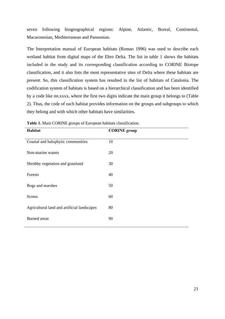
Table 1. Main CORINE groups of European habitats classification.
Habitat CORINE group
Coastal and halophytic communities 10
Non-marine waters 20
Shrubby vegetation and grassland 30
Forests 40
Bogs and marshes 50
Screes 60
Agricultural land and artificial landscapes 80
Burned areas 90
22
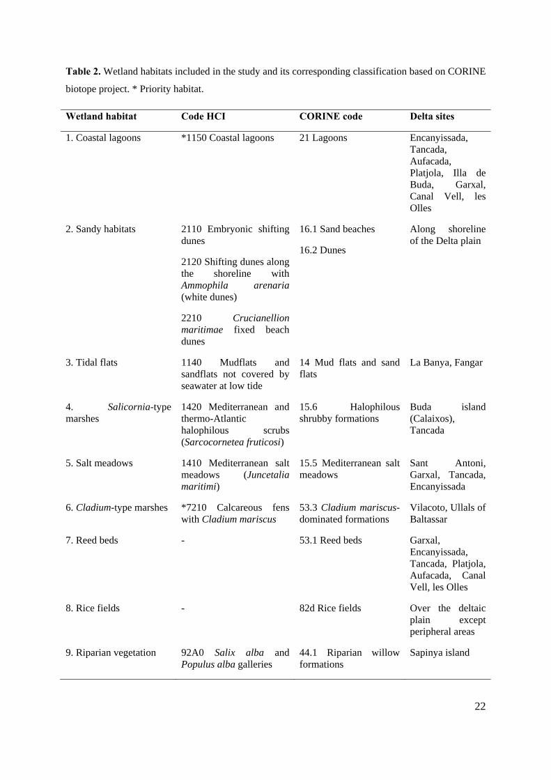
Table 2. Wetland habitats included in the study and its corresponding classification based on CORINE
biotope project. * Priority habitat.
Wetland habitat Code HCI CORINE code Delta sites
1. Coastal lagoons *1150 Coastal lagoons 21 Lagoons Encanyissada, Tancada, Aufacada, Platjola, Illa de Buda, Garxal, Canal Vell, les Olles
2. Sandy habitats 2110 Embryonic shifting dunes
2120 Shifting dunes along the shoreline with Ammophila arenaria (white dunes)
2210 Crucianellion maritimae fixed beach dunes
16.1 Sand beaches
16.2 Dunes
Along shoreline of the Delta plain
3. Tidal flats 1140 Mudflats and sandflats not covered by seawater at low tide
14 Mud flats and sand flats
La Banya, Fangar
4. Salicornia-type marshes
1420 Mediterranean and thermo-Atlantic halophilous scrubs (Sarcocornetea fruticosi)
15.6 Halophilous shrubby formations
Buda island (Calaixos), Tancada
5. Salt meadows 1410 Mediterranean salt meadows (Juncetalia maritimi)
15.5 Mediterranean salt meadows
Sant Antoni, Garxal, Tancada, Encanyissada
6. Cladium-type marshes *7210 Calcareous fens with Cladium mariscus
53.3 Cladium mariscus-dominated formations
Vilacoto, Ullals of Baltassar
7. Reed beds - 53.1 Reed beds Garxal, Encanyissada, Tancada, Platjola, Aufacada, Canal Vell, les Olles
8. Rice fields - 82d Rice fields Over the deltaic plain except peripheral areas
9. Riparian vegetation 92A0 Salix alba and Populus alba galleries
44.1 Riparian willow formations
Sapinya island
23
LegendCoastal lagoons (1150)
Sandy habitats (dunes and beaches) (2110, 2120, 2210)
Tidal flats (1140)
Salicornia-type marshes (1420)
Salt meadows (1410)
Cladium fens (7210)
Reed beds (53.1)
Rice fields (82d)
Riparian vegetation (92A0)
Ebro river
Human settlements0 5 102,5km.
´
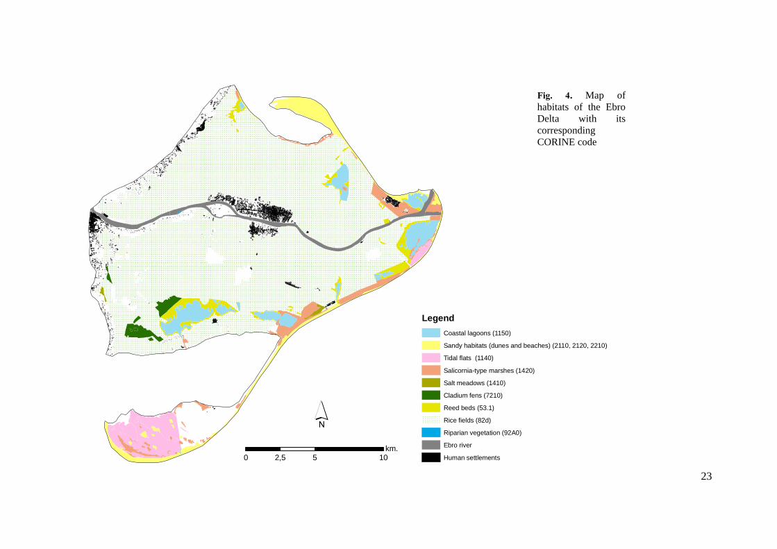
Fig. 4. Map of habitats of the Ebro Delta with its corresponding CORINE code
24
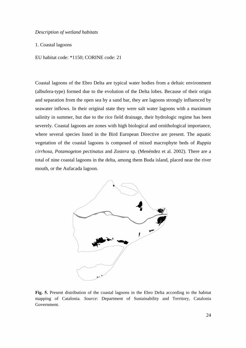
Description of wetland habitats
1. Coastal lagoons
EU habitat code: *1150; CORINE code: 21
Coastal lagoons of the Ebro Delta are typical water bodies from a deltaic environment
(albufera-type) formed due to the evolution of the Delta lobes. Because of their origin
and separation from the open sea by a sand bar, they are lagoons strongly influenced by
seawater inflows. In their original state they were salt water lagoons with a maximum
salinity in summer, but due to the rice field drainage, their hydrologic regime has been
severely. Coastal lagoons are zones with high biological and ornithological importance,
where several species listed in the Bird European Directive are present. The aquatic
vegetation of the coastal lagoons is composed of mixed macrophyte beds of Ruppia
cirrhosa, Potamogeton pectinatus and Zostera sp. (Menéndez et al. 2002). There are a
total of nine coastal lagoons in the delta, among them Buda island, placed near the river
mouth, or the Aufacada lagoon.
Fig. 5. Present distribution of the coastal lagoons in the Ebro Delta according to the habitat mapping of Catalonia. Source: Department of Sustainability and Territory, Catalonia Government.
25
2. Sandy habitats (dunes and beaches)
EU habitat code: 2110, 2120, 2210; CORINE code: 16.1, 16.2
These habitats are basically constituted by deltaic-front sand bodies. Ecologically sandy
habitats can be characterized as environment that contents low water content, low levels
of salts and organic matter and relative levels of mobility. Sandy habitats of the Ebro
Delta bring together three types of habitats of community interest related to the
substrate mobility: embryonic dunes (2110), shifting dunes with Ammophila arenaria
(2120) and fixed dunes (2210). These habitat types are considerate as transitional and
littoral sedimentary environments due to marine agents produce largely the mobilization
of its soils. Then, they are associated with littoral transfer process. The extension of this
habitat in both hemideltas is unequal. The main reason is the different orientation of the
outer coast with respect to prevailing winds (NW). Thus, the most representative area of
beaches and dunes systems is located in the northern hemidelta: Marquesa beach-Garxal
and Punta del Fangar.
Fig. 6. Present distribution of the sandy habitats (dunes and beaches) in the Ebro Delta according to the habitat mapping of Catalonia. Source: Department of Sustainability and Territory, Catalonia Government.
26
3. Tidal flats
EU habitat code: 1140; CORINE code: 14
Flat coastal areas, devoid of terrestrial vascular plants and usually colonised by blue-
green algae and diatoms. This habitat occupies coastal sands and muds and their
associated coastal lagoons that experience recurrent episodes of flooding and drying. It
is particularly well developed and forms the greatest extension in the Alfacs Peninsula,
formed by la Banya spit and Trabucador barrier. This area is very sandy, and flooding
periods are frequent due the strong northwestern winds, which results in a vertical
stratification of physicochemical gradients between the aqueous interface and the solid
substrate (Mir et al. 2000).
Fig. 7. Present distribution of the tidal flats in the Ebro Delta according to the habitat mapping of Catalonia. Source: Department of Sustainability and Territory, Catalonia Government.
27
4. Salicornia-type marshes
EU Habitat code: 1420; CORINE code: 15.6
Low shrubby expanses of woody glassworts which in the Ebro Delta are dominated by
succulent perennial species of the genus Sarcocornia and Arthrocnemum. Within the
water salinity gradient of marshes, salt marshes are the wetlands with major influence of
marine water. In them, the connexion to freshwater is limited, except for those zones
that are receiving water inflows from of adjacent rice fields. Depending on rainfall,
evaporation and tidal exchange, the salinity pattern may differ through the year. The
differences of these factors can influence the ecological and physical traits of each
marsh, such us vegetal communities (halophytic and hydrophytic), net primary
productivity or accretion and subsidence rates. Buda Island is the most representative
Arthrocnemum-type marsh in the Delta.
Fig. 8. Present distribution of the Salicornia-type marshes in the Ebro Delta according to the habitat mapping of Catalonia. Source: Department of Sustainability and Territory, Catalonia Government.
28
5. Salt meadows
EU Habitat code: 1410; CORINE code: 15.5
This habitat is characterized by the presence of Juncus acutus and Juncus maritimus as
the most representative plant. These taxa withstand high soil humidity and for this
reason grow in drenched and/or periodically submersed soils. However, the habitat finds
its ecological optimum in sites occurring at least a few centimetres higher than the
average soil water level. In the Ebro Delta, it grows in scattered inland sites where soil
elevation is higher than those of the halophilous scrub. Regarding salinity, this habitat
forms a transitional stage between salt marshes Salicornia-type and habitats lacking
halophytic vegetation. In the Ebro Delta, the salt meadows can form intermediate stands
with halophilous scrubs. According to Curcó et al. (1995) this terrestrial habitat have
been drastically reduced in relation to their potential surface area since that area has
been impounded by the rice fields.
Fig. 9. Present distribution of the salt meadows in the Ebro Delta according to the habitat mapping of Catalonia. Source: Department of Sustainability and Territory, Catalonia Government.
29
6. Cladium-type marshes
EU Habitat code: 7210; CORINE code: 16.2112
This habitat type is the only one the wetland habitats considered that constitute a
priority habitat in the Ebro Delta. Within the fresh water ecosystems, the presence of
Cladium-type marshes was originally associated with underground freshwater springs in
karstic zones (Ullals) or in elevated zones with recurrent flooding events. Nowadays the
most representative zone of this habitat in the Delta is in the Vilacoto area at the east of
the Encanyissada lagoon. In this habitat the presence of dense helophytic communities
dominated by Cladium mariscus, Phragmites australis and Scirpus maritimus is linked
with a superficial peat layer and a significant input of underground water; this fact allow
the submersion of the base of the plant during most of the year.
Fig. 10. Present distribution of the Cladium-type marshes in the Ebro Delta according to the habitat mapping of Catalonia. Source: Department of Sustainability and Territory, Catalonia Government.
30
7. Reed beds
EU Habitat code: - ;CORINE code: 53.1
The habitat occurs near lagoons, channels or other wetland types which receive direct
fresh water influence from the rice fields and the river. It occurs in still, fresh or
brackish water. Within the Ebro Delta, natural colonies of Phragmites australis develop
in the Garxal area, which is subjected to the direct influence of the riverine processes.
Along the south edge of the lagoon there is an intermediate belt of brackish reedswamp
dominated by Phragmites and Juncus species. Over the Delta plain, this habitat has
spread along the margins of the coastal lagoons and bays due to hydrological changes
caused by rice cultivation mainly.
Fig. 11. Present distribution of the reed beds in the Ebro Delta according to the habitat mapping of Catalonia. Source: Department of Sustainability and Territory, Catalonia Government.
31
8. Rice fields
EU Habitat code:- ; CORINE code: 82d
This habitat is the dominant landscape of the Delta as a result of a large agricultural
occupation process that has led an actual coverage of near the 70% of the deltaic plain.
Despite being a humanized environment and classified as artificial landscape for
CORINE Biotope project, the rice fields constitute a aquatic matrix that link fluvial,
lagoon and marine ecosystems. During the rice inundation period (May-December) this
habitat acts as an authentic aquatic ecosystem which offers zones of feeding and resting
to aquatic birds. Nevertheless, the inflow of huge amounts of fresh water into the fields
has been an important factor in alterating the hydrology of the Delta, as well as causing
loss of wetlands habitats and loss of elevation of the deltaic plain.
Fig. 12. Present distribution of the rice fields in the Ebro Delta according to the habitat mapping of Catalonia. Source: Department of Sustainability and Territory, Catalonia Government.
32
9. Riparian vegetation
EU habitat code: 92A0; CORINE code: 44.1
This type of habitat is found growing in the Sapinya Island. According to CORINE land
cover, this is the only patch of riparian vegetation present in the Ebro Delta. Under
natural conditions, the lower Ebro River was bordered by riparian forest along its
levees. Generally, this habitat types inhabited in the fluvial levees in mean elevation
range of 2 and 4 m above sea water level. Flooding events in these areas only occurred
when the river overflowed large flows, but due to construction of the dam system along
Ebro river watershed the river flow has been drastically laminated. Coupled with human
colonization of delta plain in terms of agricultural purposes, which was more significant
in these higher zones, the riparian habitats have a relictual distribution.
Fig. 13. Present distribution of the riparian vegeation in the Ebro Delta according to the habitat
mapping of Catalonia. Source: Department of Sustainability and Territory, Catalonia
Government.
33
3.4 The independent variables: elevation and distances to hydrologic boundaries
The Ebro Delta and the Mediterranean deltaic systems generally have a complex
structure and its functioning depends on hydrologic, geologic and climatic factors. The
diversity of habitats in the area of study is high, forming a set of environments that are
river- and marine-dominated. The first factor has lost importance due to the dam
construction along the Ebro River watershed concerning the reduction of near the 99%
in the particulate sediments of the lower river. Today, the hydrological conditions in
some salt marshes of the Delta are dominated by inputs of seawater through outlet
channels, much more than riverine influence, being the agricultural runoff the factor that
is altering the natural conditions (except in the river mouth area, Garxal). The
topographical factor plays a key role in the Ebro Delta since about 40% of the plain
surface lies under 0,5 meters above mean sea level (Ibàñez et al. 1996). In addition,
hydrological factors are highly correlated with the variation of soil elevation that will
determine frequency and duration of the inundation events. The distribution and
composition of lagoon-marshes complexes depends strongly on this terrain variable.
Thus, river lévées are the highest parts of the Delta, and under natural conditions, are
vegetated by riparian forests such as Populus and Salix galleries. These habitats are
flooded only during high discharge. Outside these areas are fresh, brackish or salt
marshes, depending on factors such elevation, inputs of upland runoff, riverine
influence, marine influence or soil drainage. Regarding vegetation marsh zonation, in
some cases there is a clear vegetation transition related with soil salinity and water
regime (Silvestri et al. 2005). The link between these terrain factors and vegetal
communities is one of the research questions of this study.
The independent variables included in this study for assessing the potential distribution
of the wetland habitats have been surface elevation, distance to hydrologic alterations
and distance to river/sea influence. The last approximation was assessed by the
combination of several distances which are associated with the hydrologic boundaries of
the Delta plain and will serve to extract influence of the flooding regime as an indirect
way. The hydrologic alteration approach includes all of the elements on the deltaic
34
landscape that have resulted from human activity, mainly roads, irrigation channels and
rice fields.
Table 3. List of terrain predictors included in the study.
Terrain variable Abbreviation Description Source
Surface elevation ALT Terrain altitude of the delta plain
Digital elevation model 1x1 m (Base cartogràfica de l’Institut Cartogràfic de Catalunya)
Distances to river/sea influence
- Outer coast OC External shoreline Topographical map 1, 25.000 (ICC)
- Inner border IB Inner side of deltaic plain Topographical map and ortophotomaps (ICC) 1, 25.000
- River channel RC Ebro river course and its levees
Topographical map 1, 25.000 (ICC)
- Lagoon LAG Coastal lagoons Topographical map 1, 25.000 (ICC)
- Bay BAY Coastal marine water bodies partially closed
Topographical map 1, 25.000 (ICC)
- Former river arms
FR Ancient river courses: riet Fondo, riet de Zaida and riet Vell
Digital elevation model (ICC)
- River mouth RM Current mouth of the Ebro river
Topographical map 1, 25.000 (ICC)
Distances to hydrologic alteration
- Roads ROAD Roads and paths constructed over the Delta plain
Topographical map 1, 25.000 (ICC)
- Channels CHAN Network of channels for irrigation and drainage waters from rice fields
Topographical map 1, 25.000 (ICC)
- Rice fields RF Agricultural crops of rice CORINE land cover (Department of Sustainability and Territory)
35
LegendEbro river
Coastal lagoons
Bay
Former river arms
River mouth
Outer coast
Inner border0 5 102,5km.
´
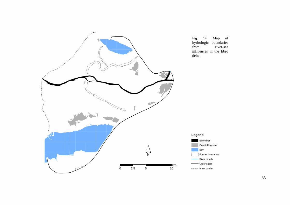
Fig. 14. Map of hydrologic boundaries from river/sea influences in the Ebro delta.
36
LegendEbro riverCoastal lagoonsChannelsRoadsRice fields5 0 52,5
km.
´
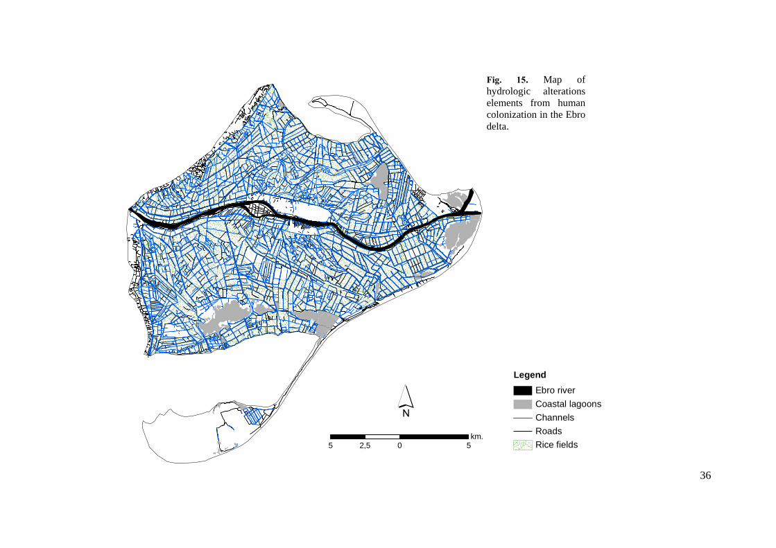
Fig. 15. Map of hydrologic alterations elements from human colonization in the Ebro delta.
37
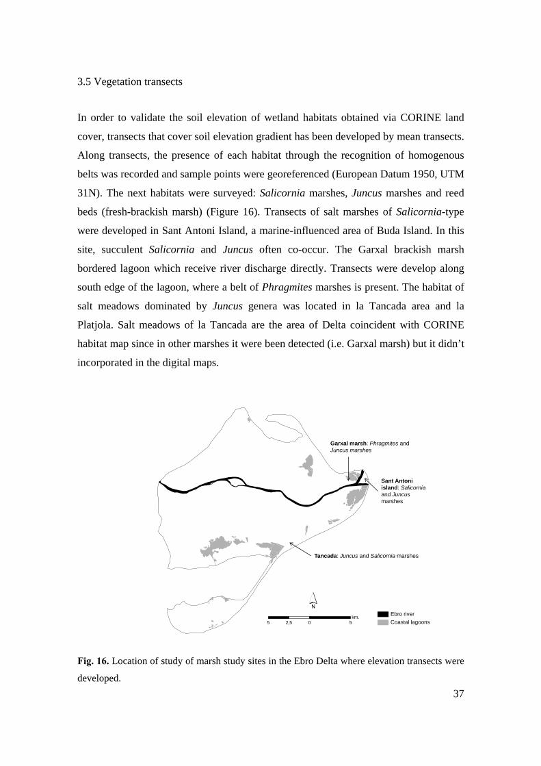
3.5 Vegetation transects
In order to validate the soil elevation of wetland habitats obtained via CORINE land
cover, transects that cover soil elevation gradient has been developed by mean transects.
Along transects, the presence of each habitat through the recognition of homogenous
belts was recorded and sample points were georeferenced (European Datum 1950, UTM
31N). The next habitats were surveyed: Salicornia marshes, Juncus marshes and reed
beds (fresh-brackish marsh) (Figure 16). Transects of salt marshes of Salicornia-type
were developed in Sant Antoni Island, a marine-influenced area of Buda Island. In this
site, succulent Salicornia and Juncus often co-occur. The Garxal brackish marsh
bordered lagoon which receive river discharge directly. Transects were develop along
south edge of the lagoon, where a belt of Phragmites marshes is present. The habitat of
salt meadows dominated by Juncus genera was located in la Tancada area and la
Platjola. Salt meadows of la Tancada are the area of Delta coincident with CORINE
habitat map since in other marshes it were been detected (i.e. Garxal marsh) but it didn’t
incorporated in the digital maps.
Ebro riverCoastal lagoons5 0 52,5
km.
´
Tancada: Juncus and Salicornia marshes
Sant Antoni island: Salicorniaand Juncusmarshes
Garxal marsh: Phragmites andJuncus marshes
Fig. 16. Location of study of marsh study sites in the Ebro Delta where elevation transects were
developed.
38
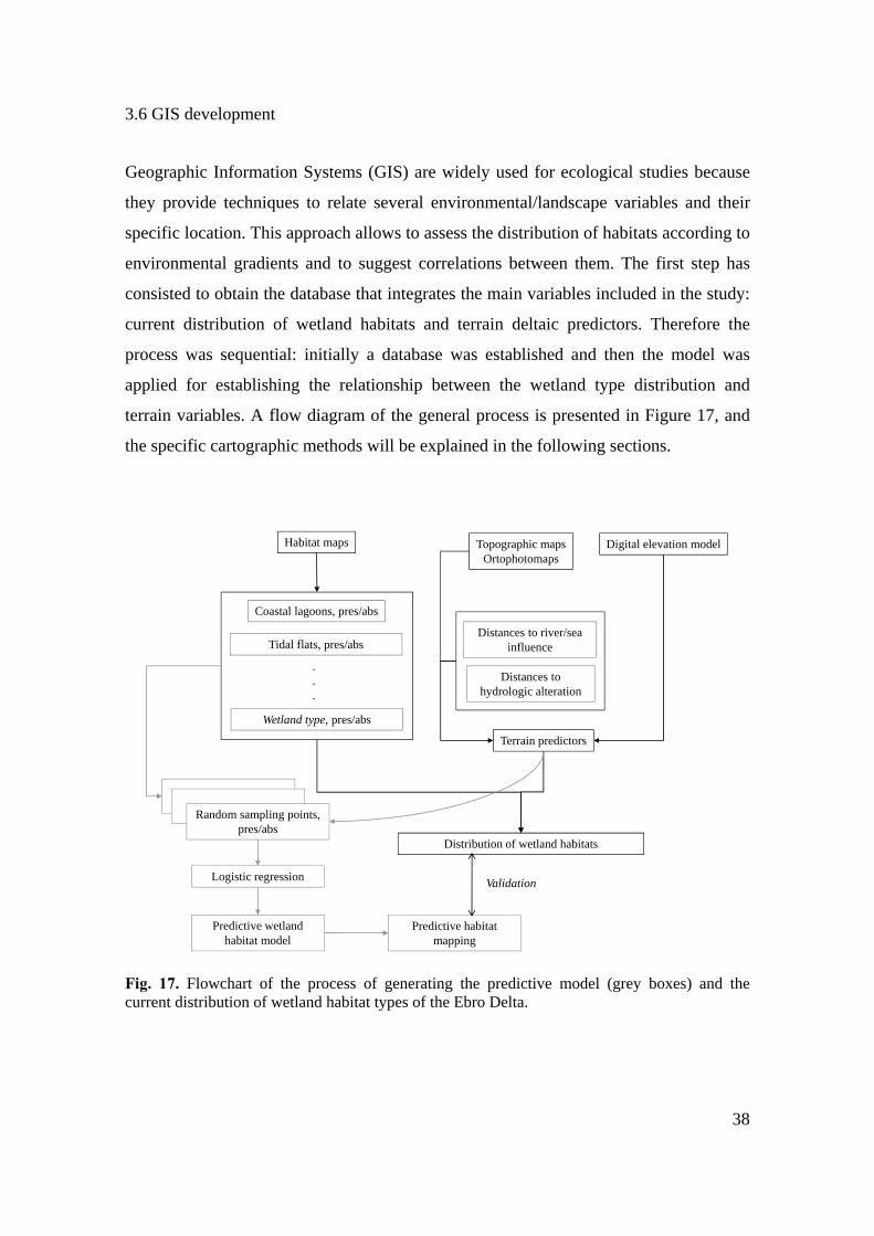
3.6 GIS development
Geographic Information Systems (GIS) are widely used for ecological studies because
they provide techniques to relate several environmental/landscape variables and their
specific location. This approach allows to assess the distribution of habitats according to
environmental gradients and to suggest correlations between them. The first step has
consisted to obtain the database that integrates the main variables included in the study:
current distribution of wetland habitats and terrain deltaic predictors. Therefore the
process was sequential: initially a database was established and then the model was
applied for establishing the relationship between the wetland type distribution and
terrain variables. A flow diagram of the general process is presented in Figure 17, and
the specific cartographic methods will be explained in the following sections.
Habitat maps
Coastal lagoons, pres/abs
Topographic mapsOrtophotomaps
Digital elevation model
Distances to river/sea influence
Distances to hydrologic alteration
Terrain predictors
Distribution of wetland habitats
Tidal flats, pres/abs
Wetland type, pres/abs
.
.
.
Logistic regression
Predictive wetland habitat model
Random sampling points, pres/abs
Predictive habitat mapping
Validation
Fig. 17. Flowchart of the process of generating the predictive model (grey boxes) and the current distribution of wetland habitat types of the Ebro Delta.
39
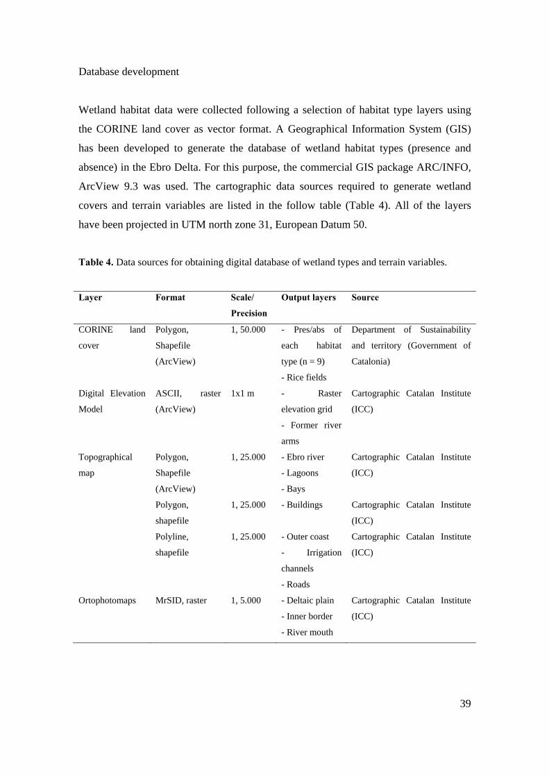
Database development
Wetland habitat data were collected following a selection of habitat type layers using
the CORINE land cover as vector format. A Geographical Information System (GIS)
has been developed to generate the database of wetland habitat types (presence and
absence) in the Ebro Delta. For this purpose, the commercial GIS package ARC/INFO,
ArcView 9.3 was used. The cartographic data sources required to generate wetland
covers and terrain variables are listed in the follow table (Table 4). All of the layers
have been projected in UTM north zone 31, European Datum 50.
Table 4. Data sources for obtaining digital database of wetland types and terrain variables.
Layer Format Scale/
Precision
Output layers Source
CORINE land
cover
Polygon,
Shapefile
(ArcView)
1, 50.000 - Pres/abs of
each habitat
type (n = 9)
- Rice fields
Department of Sustainability
and territory (Government of
Catalonia)
Digital Elevation
Model
ASCII, raster
(ArcView)
1x1 m - Raster
elevation grid
- Former river
arms
Cartographic Catalan Institute
(ICC)
Topographical
map
Polygon,
Shapefile
(ArcView)
1, 25.000 - Ebro river
- Lagoons
- Bays
Cartographic Catalan Institute
(ICC)
Polygon,
shapefile
1, 25.000 - Buildings Cartographic Catalan Institute
(ICC)
Polyline,
shapefile
1, 25.000 - Outer coast
- Irrigation
channels
- Roads
Cartographic Catalan Institute
(ICC)
Ortophotomaps MrSID, raster 1, 5.000 - Deltaic plain
- Inner border
- River mouth
Cartographic Catalan Institute
(ICC)
40
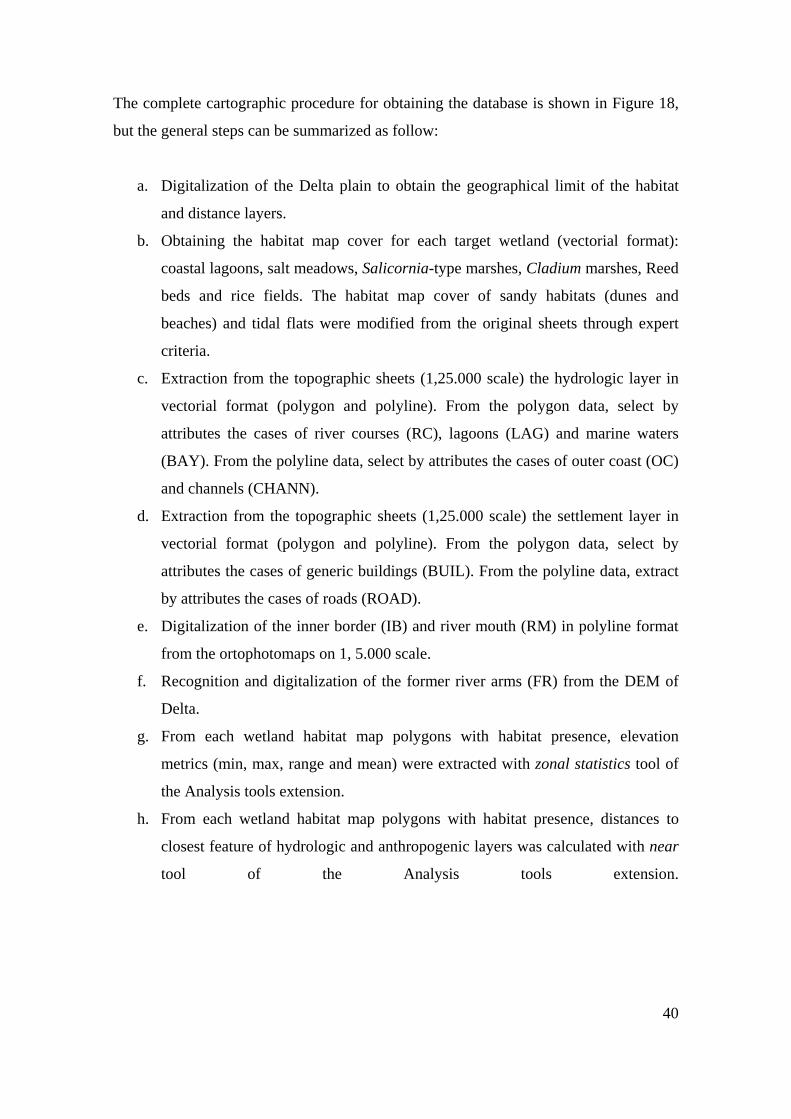
The complete cartographic procedure for obtaining the database is shown in Figure 18,
but the general steps can be summarized as follow:
a. Digitalization of the Delta plain to obtain the geographical limit of the habitat
and distance layers.
b. Obtaining the habitat map cover for each target wetland (vectorial format):
coastal lagoons, salt meadows, Salicornia-type marshes, Cladium marshes, Reed
beds and rice fields. The habitat map cover of sandy habitats (dunes and
beaches) and tidal flats were modified from the original sheets through expert
criteria.
c. Extraction from the topographic sheets (1,25.000 scale) the hydrologic layer in
vectorial format (polygon and polyline). From the polygon data, select by
attributes the cases of river courses (RC), lagoons (LAG) and marine waters
(BAY). From the polyline data, select by attributes the cases of outer coast (OC)
and channels (CHANN).
d. Extraction from the topographic sheets (1,25.000 scale) the settlement layer in
vectorial format (polygon and polyline). From the polygon data, select by
attributes the cases of generic buildings (BUIL). From the polyline data, extract
by attributes the cases of roads (ROAD).
e. Digitalization of the inner border (IB) and river mouth (RM) in polyline format
from the ortophotomaps on 1, 5.000 scale.
f. Recognition and digitalization of the former river arms (FR) from the DEM of
Delta.
g. From each wetland habitat map polygons with habitat presence, elevation
metrics (min, max, range and mean) were extracted with zonal statistics tool of
the Analysis tools extension.
h. From each wetland habitat map polygons with habitat presence, distances to
closest feature of hydrologic and anthropogenic layers was calculated with near
tool of the Analysis tools extension.
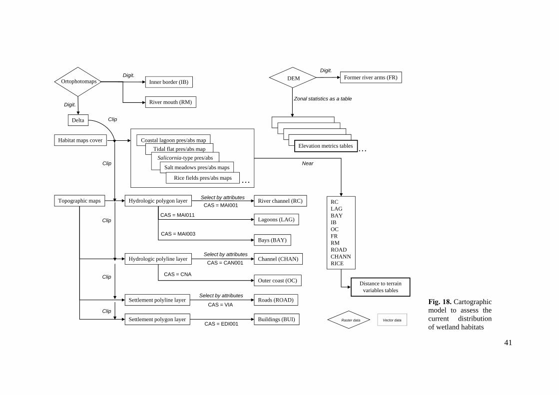
41
Ortophotomaps
Habitat maps cover
Raster data Vector data
Inner border (IB)
Digit.
Digit.
Topographic maps Hydrologic polygon layer River channel (RC)
Channel (CHAN)
Outer coast (OC)
Lagoons (LAG)
Bays (BAY)
Select by attributes
CAS = MAI003
CAS = MAI001
CAS = MAI011
Hydrologic polyline layerSelect by attributes
CAS = CAN001
Clip
Clip
CAS = CNA
Settlement polyline layer Roads (ROAD)Select by attributes
CAS = VIA
Clip
DEMDigit.
Former river arms (FR)
Zonal statistics as a table
Elevation metrics tablesElevation metrics tables
Elevation metrics tablesElevation metrics tables
Elevation metrics tables …
Delta
River mouth (RM)
Clip
Near
Coastal lagoon pres/abs mapTidal flat pres/abs map
Salicornia-type pres/abs mapsSalt meadows pres/abs maps
…Rice fields pres/abs maps
RCLAGBAYIBOCFRRMROADCHANNRICE
Distance to terrain variables tables
Settlement polygon layerCAS = EDI001
Buildings (BUI)Clip
Fig. 18. Cartographic model to assess the current distribution of wetland habitats
42
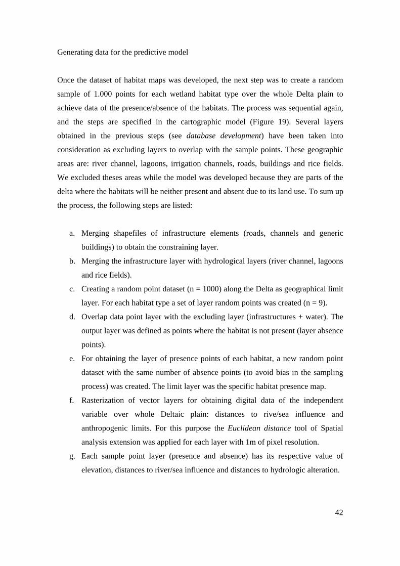
Generating data for the predictive model
Once the dataset of habitat maps was developed, the next step was to create a random
sample of 1.000 points for each wetland habitat type over the whole Delta plain to
achieve data of the presence/absence of the habitats. The process was sequential again,
and the steps are specified in the cartographic model (Figure 19). Several layers
obtained in the previous steps (see database development) have been taken into
consideration as excluding layers to overlap with the sample points. These geographic
areas are: river channel, lagoons, irrigation channels, roads, buildings and rice fields.
We excluded theses areas while the model was developed because they are parts of the
delta where the habitats will be neither present and absent due to its land use. To sum up
the process, the following steps are listed:
a. Merging shapefiles of infrastructure elements (roads, channels and generic
buildings) to obtain the constraining layer.
b. Merging the infrastructure layer with hydrological layers (river channel, lagoons
and rice fields).
c. Creating a random point dataset (n = 1000) along the Delta as geographical limit
layer. For each habitat type a set of layer random points was created (n = 9).
d. Overlap data point layer with the excluding layer (infrastructures + water). The
output layer was defined as points where the habitat is not present (layer absence
points).
e. For obtaining the layer of presence points of each habitat, a new random point
dataset with the same number of absence points (to avoid bias in the sampling
process) was created. The limit layer was the specific habitat presence map.
f. Rasterization of vector layers for obtaining digital data of the independent
variable over whole Deltaic plain: distances to rive/sea influence and
anthropogenic limits. For this purpose the Euclidean distance tool of Spatial
analysis extension was applied for each layer with 1m of pixel resolution.
g. Each sample point layer (presence and absence) has its respective value of
elevation, distances to river/sea influence and distances to hydrologic alteration.

43
h. The extraction of variables was executed with the Sample tool for obtaining the
final data matrix with the 11 independent variables and presence/absence of each
habitat type for total sample points.
44
Channel (CHAN)
Roads (ROAD)
River channel (RC)
Lagoons (LAG)
Buildings (BUI)Constraining layer
Delta
Create random points
model_pointsn = 1000
absence_points
n points = a
absence_pointsabsence_points
absence_pointsabsence_points
Coastal lagoon pres mapTidal flat pres map
Salicornia-type pres maps
Salt meadows pres maps
…Rice fields pres maps
Create random points
n = aabsence_points
absence_pointsabsence_points
absence_pointspresence_points
Erase
Rice fields (RICE)
RCLAGBAYIBOCFRRMROADCHANNRICE
RCLAGBAY
IBOCFRRM
ROADCHANN
RICEZ
Coastal lagoonTidal flat
Salicornia-type
Salt meadows
Rice fields
…Data matrix
for eachhabitat type
Sample
Sample
Euclidean distance
1x1m
Fig. 19. Cartographic model to generate sample points and extract the metrics for predictive wetland model
45
3.7 Statistical analysis
For each wetland habitat type, the presence/absence points and its respective terrain metrics
(elevation, distances to river/sea influence and distances to hydrologic alteration sources) was
determined with GIS-approach as described in the previous sections. PCA analysis was
initially performed to study the overall relations between elevation and distance variables.
Regression scores were extracted to analyze each wetland habitat pattern. Moreover,
differences on variables between wetland habitats were assessed for achieving their ranges
into the hydrological influence and soil altitude gradients. All the environmental independent
variables were checked previously for normality and linearity. All the variables required
natural logarithmic transformation to meet these parametric assumptions. Differences on
vertical soil elevation between habitats assessed by CORINE land cover and mean transects
was tested by Mann-Whitney test. Correlation analysis between elevation metrics (min, max,
range and mean) and distances was performed to check the independence of the variables. All
the statistical analyses were performed using SPSS v18.0 for Windows package.
Logistic multiple regression predictive model
As habitat map points are categorical variables (presence or absence), logistic regression is
proposed for predicting occurrence of wetland habitat types from topographical deltaic
variables (independent variables)(Hosmer and Lemeshow 2000). LMR is adequate because
the dependent variable is dichotomous (presence/absence) and the model admits non-
Gaussian independent variables (Franklin 1995). As explained, several authors proposed to
use equal number of presence and absence points for developing logistic method to avoid bias
(Felicísimo 2003; Narumalani et al. 1997). The foundation of the method is based on the
probability of occurrence of any number of classes of a dependent variable (in this study,
wetland habitat) based on explanatory variables (i.e elevation and distances). According to
Custer and Eveleigh (1986), “regression modeling involves the derivation of a mathematical
relationship between a set of independent predictor variables and a specific dependent
condition”. A multiple logistic regression analysis within the sample points generated in
previous steps resulted in an individual regression equation for each wetland habitat type.
46
Logistic regression is sensitive to extremely high correlations between variables that are
supposed to be independent (Hosmer and Lemeshow 2000). To avoid this, high correlation
between variables was eliminated by retaining only the variable with the highest explanatory
power for pairs of variables with r Pearson coefficient (r > 0,6)(Filipe et al. 2002). In the
multivariate analysis a forward stepwise was applied to each selected variable with a
probability of entry of 0,05 and removal of 0,10. The addition and exclusion of variables was
based on Wald’s test and the assessment of correlation was based on differences in the
coefficients estimated when a variables is added to the model and from partial correlation of
the estimated coefficients for p<0,001 (Zar 1999).
To assess the fit of each model, the Chi-square test and a classification table was used. This
procedure has been used by other authors (Narumalani et al. 1997; Ríos et al. 2005). The fit
test examined the deviance of the model with the constant versus the final model and rejection
was at p<0,05 significance based on a chi-square distribution. Another technique has been
used to evaluate each predictive model. The Receiver Operating Characteristic (ROC)
provides a threshold independent measure of accuracy and results in a plot of the relative
proportions of correctly classified sites over the whole range of threshold levels (Narumalani
et al. 1997; Tarkesh and Jetschke 2012). The ROC plot is obtained by plotting the sensitivity
of the model against the false positive fraction over all thresholds, being the area under the
curve (AUC) the probability that the model will distinguish correctly between observations.
An area of 1 is perfectly accurate, whereas on of 0,5 is performing a random model (no
acceptable). This fitting method has been applied in several studies of predictive vegetation
modelling (Álvarez-Arbesú and Felicísimo 2002; Felicísimo et al. 2002; Syphard and
Franklin 2010). All the statistical analyses were performed using SPSS v18.0 for Windows
package.
Model validation
The predictive model has been validated with independent data obtained by field surveys, in
which information about the presence/absence of different habitats was obtained by mean of
transects. So, the validation was applied to Salicornia marshes, salt meadows and reed beds.
47
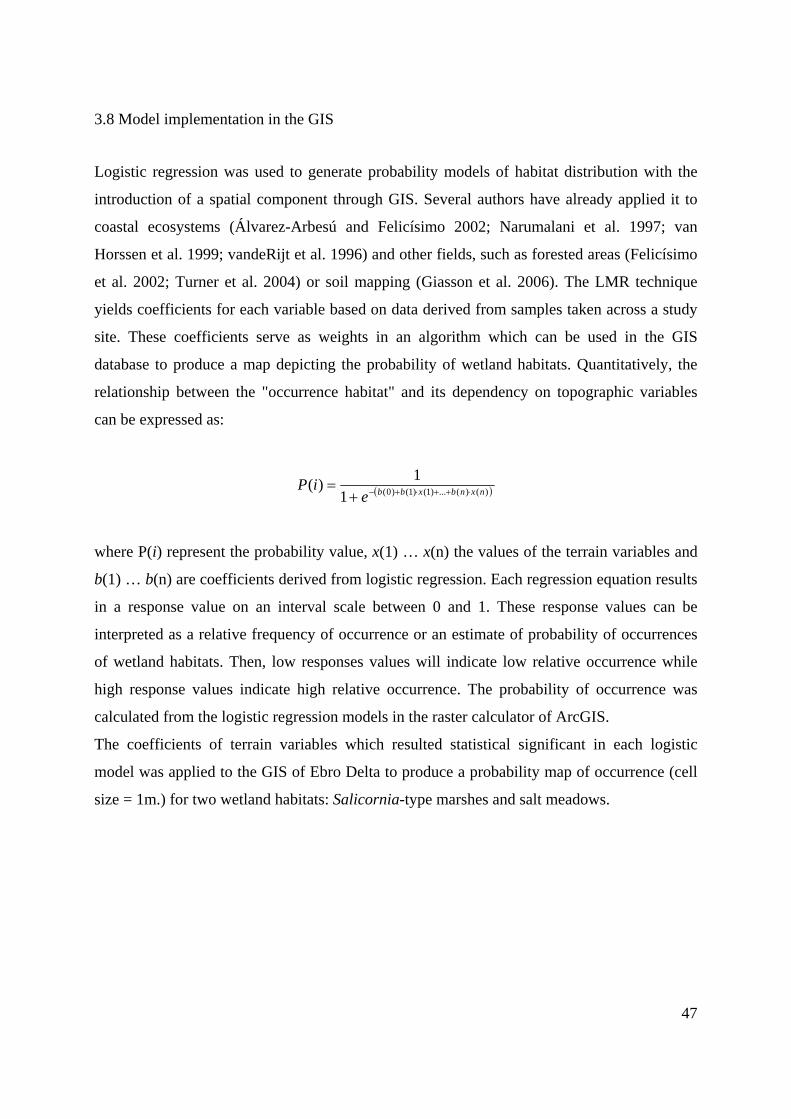
3.8 Model implementation in the GIS
Logistic regression was used to generate probability models of habitat distribution with the
introduction of a spatial component through GIS. Several authors have already applied it to
coastal ecosystems (Álvarez-Arbesú and Felicísimo 2002; Narumalani et al. 1997; van
Horssen et al. 1999; vandeRijt et al. 1996) and other fields, such as forested areas (Felicísimo
et al. 2002; Turner et al. 2004) or soil mapping (Giasson et al. 2006). The LMR technique
yields coefficients for each variable based on data derived from samples taken across a study
site. These coefficients serve as weights in an algorithm which can be used in the GIS
database to produce a map depicting the probability of wetland habitats. Quantitatively, the
relationship between the "occurrence habitat" and its dependency on topographic variables
can be expressed as:
( ))()(...)1()1()0(11)( nxnbxbbe
iP ⋅++⋅+−+=
where P(i) represent the probability value, x(1) … x(n) the values of the terrain variables and
b(1) … b(n) are coefficients derived from logistic regression. Each regression equation results
in a response value on an interval scale between 0 and 1. These response values can be
interpreted as a relative frequency of occurrence or an estimate of probability of occurrences
of wetland habitats. Then, low responses values will indicate low relative occurrence while
high response values indicate high relative occurrence. The probability of occurrence was
calculated from the logistic regression models in the raster calculator of ArcGIS.
The coefficients of terrain variables which resulted statistical significant in each logistic
model was applied to the GIS of Ebro Delta to produce a probability map of occurrence (cell
size = 1m.) for two wetland habitats: Salicornia-type marshes and salt meadows.
48
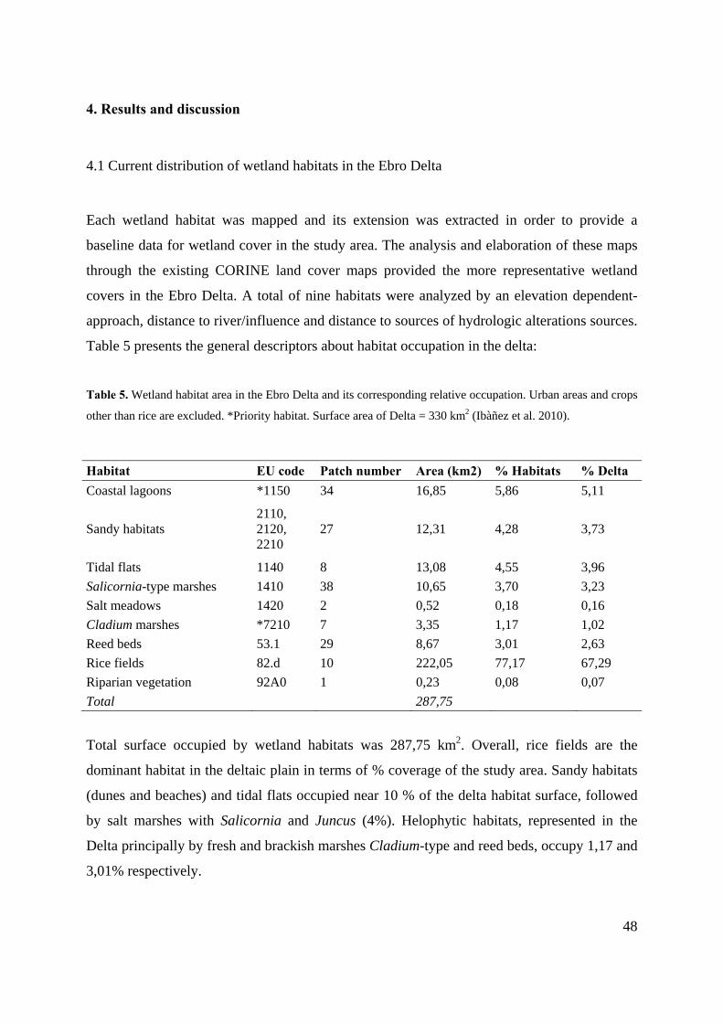
4. Results and discussion
4.1 Current distribution of wetland habitats in the Ebro Delta
Each wetland habitat was mapped and its extension was extracted in order to provide a
baseline data for wetland cover in the study area. The analysis and elaboration of these maps
through the existing CORINE land cover maps provided the more representative wetland
covers in the Ebro Delta. A total of nine habitats were analyzed by an elevation dependent-
approach, distance to river/influence and distance to sources of hydrologic alterations sources.
Table 5 presents the general descriptors about habitat occupation in the delta:
Table 5. Wetland habitat area in the Ebro Delta and its corresponding relative occupation. Urban areas and crops
other than rice are excluded. *Priority habitat. Surface area of Delta = 330 km2 (Ibàñez et al. 2010).
Habitat EU code Patch number Area (km2) % Habitats % Delta Coastal lagoons *1150 34 16,85 5,86 5,11
Sandy habitats 2110, 2120, 2210
27 12,31 4,28 3,73
Tidal flats 1140 8 13,08 4,55 3,96 Salicornia-type marshes 1410 38 10,65 3,70 3,23 Salt meadows 1420 2 0,52 0,18 0,16 Cladium marshes *7210 7 3,35 1,17 1,02 Reed beds 53.1 29 8,67 3,01 2,63 Rice fields 82.d 10 222,05 77,17 67,29 Riparian vegetation 92A0 1 0,23 0,08 0,07 Total 287,75
Total surface occupied by wetland habitats was 287,75 km2. Overall, rice fields are the
dominant habitat in the deltaic plain in terms of % coverage of the study area. Sandy habitats
(dunes and beaches) and tidal flats occupied near 10 % of the delta habitat surface, followed
by salt marshes with Salicornia and Juncus (4%). Helophytic habitats, represented in the
Delta principally by fresh and brackish marshes Cladium-type and reed beds, occupy 1,17 and
3,01% respectively.
49
Phragmites marshes (reed beds) have an important representation in the deltaic landscape
since occupy brackish (Garxal), fresh marshes (Vilacoto) and the altered margins of the salt
marshes due to agricultural runoff (Encanyissada, Aufacada). This habitat forms a great
diversity of plants associations from a physiognomic point of view due to high variability of
flooding levels and water salinity in the Delta (Curcó 2001).
Under natural conditions (i.e peat soils largely flooded by carbonate fresh waters) Cladium-
type marshes is limited to the natural wells “ullals” and some coastal lagoons that receives a
significant of fresh groundwater supply (Encanyissada, Vilacoto). The potential area of
Cladium marshes havs been modified by human activities (mainly agriculture) and its
hydrological pattern has been altered by the establishment of an extensive draining system to
lower the underground water level (Capítulo et al. 1994). This habitat is included in Annex 1
of the European Union Directive as a priority habitat type (7210 Calcareous fens with
Cladium mariscus and species of the Caricion davallianae).
The aquatic habitat of coastal lagoons is the other European priority habitat type included in
our study. Coastal lagoons of the Ebro Delta are the most representative aquatic habitats and
they occupy a higher surface area than the terrestrial habitats such as sand-dunes systems or
Phragmites beds. Their hydrologic conditions have changed over the past 100 years due to the
increment of the fresh water inputs and according Curcó and col. (1995) former coastal
lagoons occupied most their potential area and were more numerous. There is a high
variability in terms of surface of the lagoons: ranging from Garxal lagoon with 235 ha to
Encanyissada lagoon with 786 ha. The main source of variation in the coastal lagoons is their
hydrological regime which varies according to the fresh and salt water inputs. The freshest are
the west basin of the Encanyissada lagoon, les Olles and those having more connection with
the river (Garxal lagoon). The saltiest lagoons (la Tancada, Canal Vell or Buda), as other
Mediterranean coastal lagoons, have a hydrological pattern linked with seawater fluctuations
and some of them have periods of hypersalinity in summer (Badosa et al. 2006; Pérez-Ruzafa
et al. 2005).
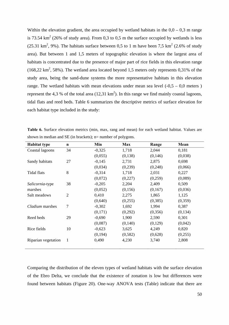
50
Within the elevation gradient, the area occupied by wetland habitats in the 0,0 – 0,3 m range
is 73.54 km2 (26% of study area). From 0,3 to 0,5 m the surface occupied by wetlands is less
(25.31 km2, 9%). The habitats surface between 0,5 to 1 m have been 7,5 km2 (2.6% of study
area). But between 1 and 1,5 meters of topographic elevation is where the largest area of
habitats is concentrated due to the presence of major part of rice fields in this elevation range
(168,22 km2, 58%). The wetland area located beyond 1,5 meters only represents 0,31% of the
study area, being the sand-dune systems the more representative habitats in this elevation
range. The wetland habitats with mean elevations under mean sea level (-0,5 – 0,0 meters )
represent the 4,3 % of the total area (12,31 km2). In this range we find mainly coastal lagoons,
tidal flats and reed beds. Table 6 summarizes the descriptive metrics of surface elevation for
each habitat type included in the study:
Table 6. Surface elevation metrics (min, max, rang and mean) for each wetland habitat. Values are
shown in median and SE (in brackets); n= number of polygons.
Habitat type n Min Max Range Mean Coastal lagoons 34 -0,325
(0,055) 1,718 (0,138)
2,044 (0,146)
0,181 (0,038)
Sandy habitats 27 -0,145 (0,034)
2,731 (0,239)
2,875 (0,248)
0,698 (0,066)
Tidal flats 8 -0,314 (0,072)
1,718 (0,227)
2,031 (0,259)
0,227 (0,089)
Salicornia-type marshes
38 -0,205 (0,052)
2,204 (0,156)
2,409 (0,167)
0,509 (0,036)
Salt meadows 2 0,410 (0,640)
2,275 (0,255)
1,865 (0,385)
1,125 (0,359)
Cladium marshes 7 -0,302 (0,171)
1,692 (0,292)
1,994 (0,356)
0,387 (0,134)
Reed beds 29 -0,690 (0,087)
1,900 (0,140)
2,590 (0,129)
0,301 (0,042)
Rice fields 10 -0,623 (0,194)
3,625 (0,582)
4,249 (0,628)
0,820 (0,255)
Riparian vegetation 1 0,490
4,230 3,740 2,808
Comparing the distribution of the eleven types of wetland habitats with the surface elevation
of the Ebro Delta, we conclude that the existence of zonation is low but differences were
found between habitats (Figure 20). One-way ANOVA tests (Table) indicate that there are
51
significant differences between the surface elevation of the wetland habitats observed.
Elevation metrics (min, max and mean) were previously log-transformed for achieving
parametric assumptions.
A B
C
Reed
beds
Rice
fields
Lagoons
Tidalflats
Cladium
Salicornia
Sand-dune
Salt meadow
s
Riparian
Reed
beds
Rice
fields
Lagoons
Tidalflats
Cladium
Salicornia
Sand-dune
Riparian
Salt meadow
s
Cladium
Reed
beds
Tidalflats
Lagoons
Salicornia
Salt m
eadows
Rice
fields
Riparian
Sand-dune
-1,000
0,000
1,000
2,000
a
b
a,b a,b a,b a,b a,b a,ba a a a,b
a,ba,b
a,b
b
a a a,ba,b a,b
b,c
b,c
c
1,000
2,000
3,000
4,000
5,000
0,000
0,500
1,000
1,500
2,000
2,500
3,000
Fig. 20. Surface elevation metrics (in meters) for each habitat type of the Ebro Delta. A: minimum, B:
maximum, C: mean. The error bars represents the standard error considering all the polygons of the
CORINE habitat map. Different letters point to significant differences (post hoc Tukey test: p < 0.05)
52
Table 7. One-way ANOVA results for the surface elevation metrics extracted from CORINE land
cover maps. Riparian vegetation was not included in the ANOVA analysis due to an insufficient
number of samples.
Elevation metrics Sum of Squares df Mean Square F Sig.
Minimum Between Groups 2,219 8 0,277 5,652 <0,000Within Groups 7,163 146 0,049 Total 9,382 154
Mean Between Groups 0,465 8 0,058 13,408 <0,000Within Groups 0,637 147 0,004 Total 1,101 155
Maximum Between Groups 1,113 8 0,139 5,566 <0,000Within Groups 3,676 147 0,025 Total 4,789 155
Range Between Groups 0,873 8 0,109 4,387 <0,000
Within Groups 3,655 147 ,025
Total 4,528 155
Lower elevations, excluding coastal lagoons, are occupied more frequency by tidal flats and
reed bed habitats. Phragmites marshes are present in the lowest mean elevation in contact
directly with coastal lagoons (Fig. 20A), as mapped in the CORINE land cover. Even though,
the minimum elevation of emergent reed beds (-0,69 m.) has to taking into account since the
growing of these communities is limited in waters of 0,3 – 0,4 m. depth (Coops et al. 1996;
Squires and Valk 1992). Although scarce in the Delta (Ibàñez et al. 2002) this habitat type
will be present in permanent or nearly flooded soils of fresh-brackish marshes.
In salty coastal environments like the Ebro Delta, salt marshes are dominated by Salicornia-
type vegetation and depending on its relative soil elevation, different genera can dominate
(Ibàñez et al. 2010). In this study, Salicornia-type habitat had a mean elevation of 0,51 ± 0,04
m. Other authors (Pont et al. 2002) have found a similar topographic distribution of these
habitats in the Rhône Delta, which range between 0,25 and 0,60 m.
A more clear variation of soil elevation at upper regions was detected between Salicornia-
type habitat and salt meadows dominated by Juncus. Even though this halophytic habitat has
been drastically reduced in the Ebro Delta, its still occupies a broad range of elevation.
Regarding salinity, salt meadows with Juncus maritimus and Juncus acutus occur in soils less
53
influenced by the underground sea water level in contrast to the exclusive halophytic
communities (fruticose salt-marshes) (Espinar 2009). Thus, significant differences in mean
soil elevation of Salicornia-type and Juncus-type environments were found (unpaired t test, p
< 0,05). Silvestri and col. (2005) found a mean elevation difference between Juncus genus
and Arthrocnemum genus of 15 cm. Our results show that given habitats are found at higher
differentiated topographic elevations.
The riparian habitat was observed at the highest mean and maximum surface elevation of the
habitats (Fig. 20.D). The only patch mapped from CORINE land cover (Sapinya Island, 24
ha) shows a mean surface elevation of 2,81 m and its elevation can be considered
representative of this habitat. This habitat is present in the fluvial levees that are the highest
areas of the Delta plain, where it should develop according to the lowest salinity levels and
eventual flooding events. Presently, the potential area of riparian vegetation of the Delta,
especially Populus and Salix genus, has been transformed into rice fields and other crops.
The humanized habitat of rice fields is present in the maximum range soil elevation extracted
by the DEM of Deltaic plain. (Fig. 20.C). While other habitat types have a narrow elevation
range (i.e tidal flats or Cladium marshes) rice fields exhibit a wide distribution, indicating a
relative indifference to soil elevation. The high surface area occupied by rice throughout the
Delta plain, from near-river lévées to the margins of the coastal lagoons has led to major part
of the topographic gradient being occupied by this habitat. Moreover, the soil elevation of the
Delta has been altered in many areas by agricultural purposes, lowering the upper zones and
filling depressions. Then, the wide range in the elevation of this habitat could be attributed to
this human factor.
Methodological constrains on DEM application
In several habitats, no consistent results have been detected in the application of high precise
Digital Elevation Model of the Ebro Delta. Coastal lagoons showed mean elevation above sea
level (0,18 m.), and its maximum elevation was placed around 1,7 m. When extracting
elevation, the presence of micro-topography like “tores” (accumulation of soil in inundation
areas that it elevates above water surface) probably result in a bias of elevation values. The
level of detail in mean elevation of tidal flats (0,23 m.) it may associated to the same issue.
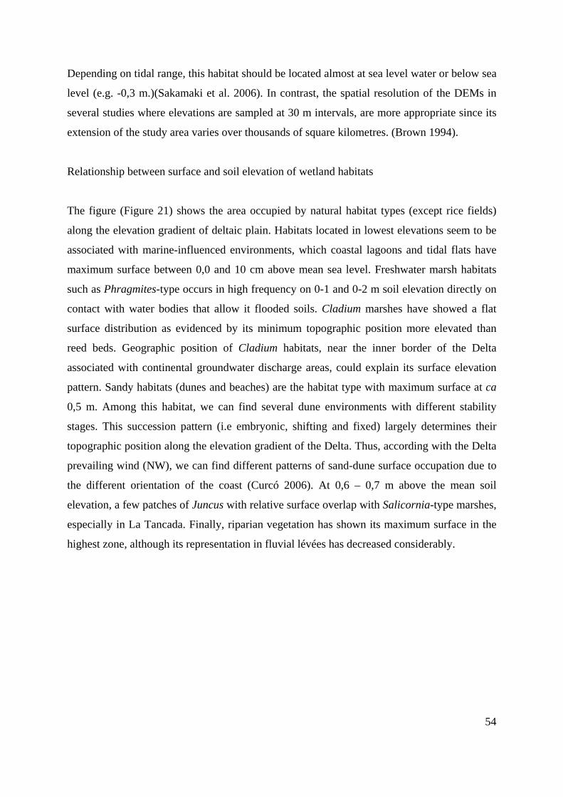
54
Depending on tidal range, this habitat should be located almost at sea level water or below sea
level (e.g. -0,3 m.)(Sakamaki et al. 2006). In contrast, the spatial resolution of the DEMs in
several studies where elevations are sampled at 30 m intervals, are more appropriate since its
extension of the study area varies over thousands of square kilometres. (Brown 1994).
Relationship between surface and soil elevation of wetland habitats
The figure (Figure 21) shows the area occupied by natural habitat types (except rice fields)
along the elevation gradient of deltaic plain. Habitats located in lowest elevations seem to be
associated with marine-influenced environments, which coastal lagoons and tidal flats have
maximum surface between 0,0 and 10 cm above mean sea level. Freshwater marsh habitats
such as Phragmites-type occurs in high frequency on 0-1 and 0-2 m soil elevation directly on
contact with water bodies that allow it flooded soils. Cladium marshes have showed a flat
surface distribution as evidenced by its minimum topographic position more elevated than
reed beds. Geographic position of Cladium habitats, near the inner border of the Delta
associated with continental groundwater discharge areas, could explain its surface elevation
pattern. Sandy habitats (dunes and beaches) are the habitat type with maximum surface at ca
0,5 m. Among this habitat, we can find several dune environments with different stability
stages. This succession pattern (i.e embryonic, shifting and fixed) largely determines their
topographic position along the elevation gradient of the Delta. Thus, according with the Delta
prevailing wind (NW), we can find different patterns of sand-dune surface occupation due to
the different orientation of the coast (Curcó 2006). At 0,6 – 0,7 m above the mean soil
elevation, a few patches of Juncus with relative surface overlap with Salicornia-type marshes,
especially in La Tancada. Finally, riparian vegetation has shown its maximum surface in the
highest zone, although its representation in fluvial lévées has decreased considerably.
55
Are
a (k
m2 )
Fig. 21. Distribution of natural habitat types as function of soil elevation and surface. Rice fields were not included in the plot.
56
Relationship between terrain variables
For the entire wetland habitats the lowest elevation, highest elevation, range elevation and
mean elevation show strong positive correlation (Pearson, p<0,01). The mean elevation has
been correlated positively with the distance to channels and negatively with distance to inner
border, lagoons, river and former river arms.
The three variables related with hydrologic alterations elements (roads, channels and rice
fields) were strongly (negatively) correlated to each other, which was expected due to their
overlapped position in the deltaic plain. Note that distance to former river arms of the Ebro
River (Riet de Zaida, Fondo and Muntells) was correlated positively with distance to rice
fields, channels and roads of the Delta. This can be explained because of these ancient courses
are largely occupied by rice fields and consequently by channels, either irrigation or drainage.
A significative (negative) correlation was found between distance to bay and river channel
that could represent a longitudinal gradient from fluvial lévées to bay (marine influence).
Distances associated with the riverine influence are also strongly correlated, mainly between
river channel and river mouth.
PCA ordination
In order to investigate the relations between all the environment variables on wetland habitats
distribution a principal component analysis (PCA) with varimax rotation was carried out
(Figure 22). Most of the analyzed variables were interdependent and have significative
correlation among them (Table correlations). The usefulness o the PCA was checked through
Kaiser-Meyer-Olkin’s (KMO) measure of adequacy sample (0,686) and Bartlett’s test of
sphericity (p<0,001). The two first axes explaining the 26% and 22% of the total variation
respectively. The minimum elevation of habitat polygons and distances to anthropogenic
elements was correlated positively with PCA axis 1. The first axis separated the patches of
wetland habitats closer to road, channels rice fields and former river arms with higher
minimum elevation than patches placed far of these elements (lower minimum elevations).
Then, the first axis summarizes the variation associated with rising elevation of wetland
habitat placed near anthropogenic elements and ancient river lévées. PCA axis 2 explains the
variation associated with maximum elevation gradient of habitat patches from interior to
exterior deltaic plain. The highest elevation of habitats patches has been correlated
57
(positively) with areas placed near the inner border of the Delta and opposites to exterior
limits of Delta (outer coast and river mouth).
The regression scores of each habitat polygon were extracted to visualize their position on the
two PCA axes. Analysis of salt meadows and riparian vegetation were not assessed due to its
lower polygons in the CORINE habitat map.
Some coastal lagoons were relatively separated on PCA axis 2: Buda lagoons were negatively
correlated with it (i.e. near from river mouth and outer coast and lower maximum elevations)
and patches of Encanyissada were correlated positively (i.e. far from river mouth and higher
maximum elevations).
Sand dunes showed patches separated along PC2. Sandy habitats correlated positively with
this axis have higher maximum elevations and are influenced by river mouth and outer coast
(e.g. Fangar dunes). While dunes/beaches oppositely placed along PCA axis 2 have shown
lower maximum elevations and were more influenced by bays and inner border (e.g.
dunes/beaches of Trabucador barrier). Tidal flats polygons have been differentiated in the
patches of Buda area (near river mouth and correlated positively with PC1) and patches of
Punta de la Banya.
The patches of Salicornia habitats were relatively separated along PCA axis 2. Then,
Salicornia-type marshes of Buda were different of polygons placed in la Banya given that the
last showed negative correlation with elevation and distance to river mouth. It means that
while there are some patches of Salicornia with lower maximum elevations located near the
bay, oppositely other groups with higher maximum elevations were placed near river mouth.
The reed beds were grouped according to PCA axis 2 mainly. Then, polygons with lower
maximum elevations and near to river mouth and outer coast were correlated negatively with
PC2 (i.e. reed beds of Buda lagoon as representative place). While patches of Phragmites
located in la Tancada seems to be associated with higher maximum elevations and greater
distances to these limits than either Buda or Garxal reed beds (positively correlated with
PC2). PCA axis 1 explains another source of variation related with reed beds distribution.
This axis separates groups of reed beds placed far from anthropogenic and former river arms
which can cause uprising elevation effect (higher minimum elevations).
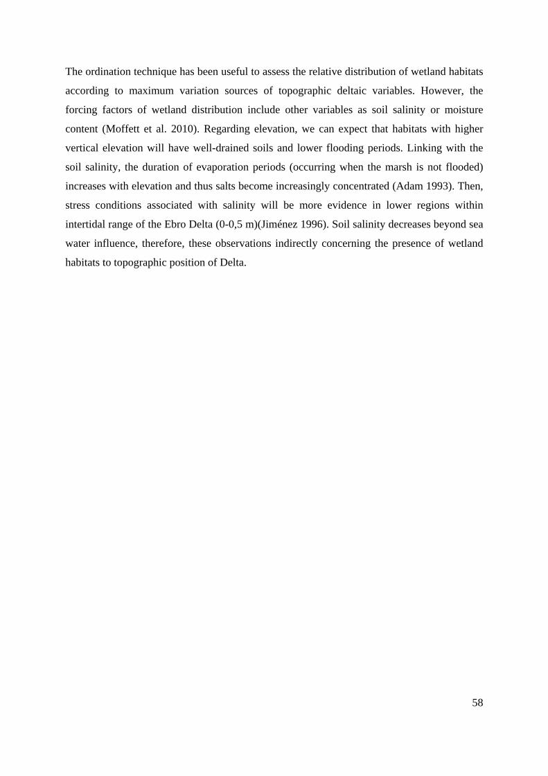
58
The ordination technique has been useful to assess the relative distribution of wetland habitats
according to maximum variation sources of topographic deltaic variables. However, the
forcing factors of wetland distribution include other variables as soil salinity or moisture
content (Moffett et al. 2010). Regarding elevation, we can expect that habitats with higher
vertical elevation will have well-drained soils and lower flooding periods. Linking with the
soil salinity, the duration of evaporation periods (occurring when the marsh is not flooded)
increases with elevation and thus salts become increasingly concentrated (Adam 1993). Then,
stress conditions associated with salinity will be more evidence in lower regions within
intertidal range of the Ebro Delta (0-0,5 m)(Jiménez 1996). Soil salinity decreases beyond sea
water influence, therefore, these observations indirectly concerning the presence of wetland
habitats to topographic position of Delta.
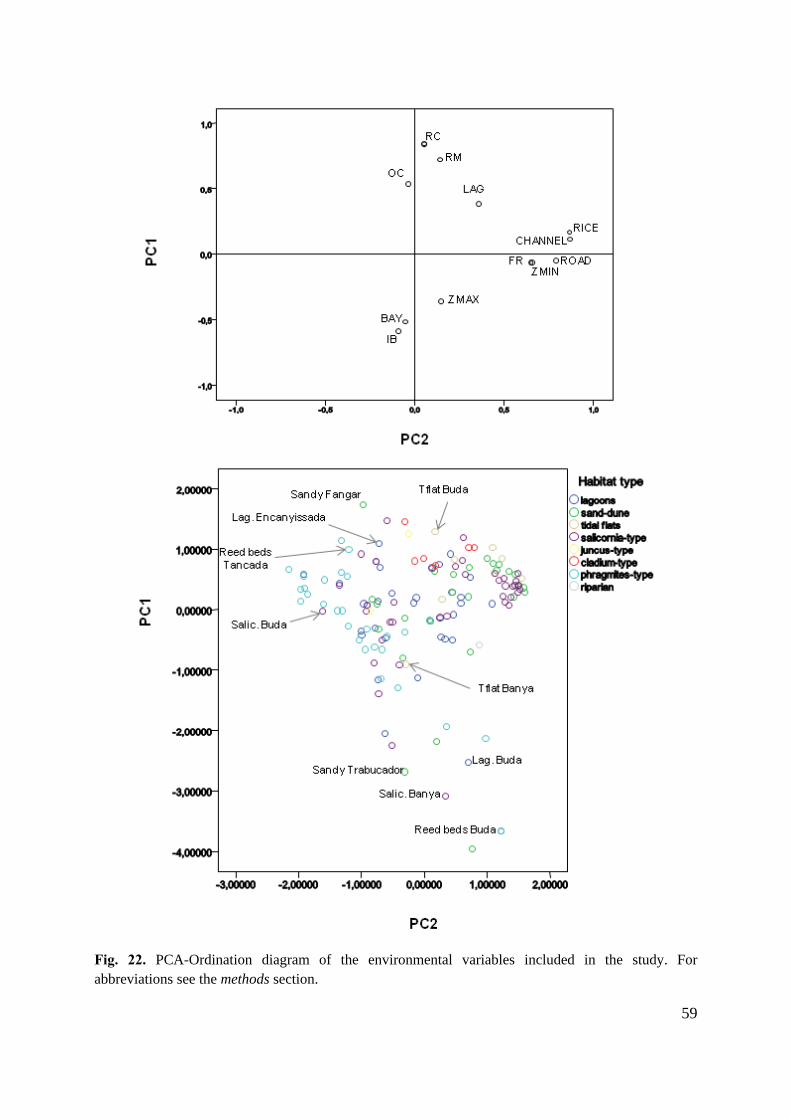
59
Fig. 22. PCA-Ordination diagram of the environmental variables included in the study. For abbreviations see the methods section.
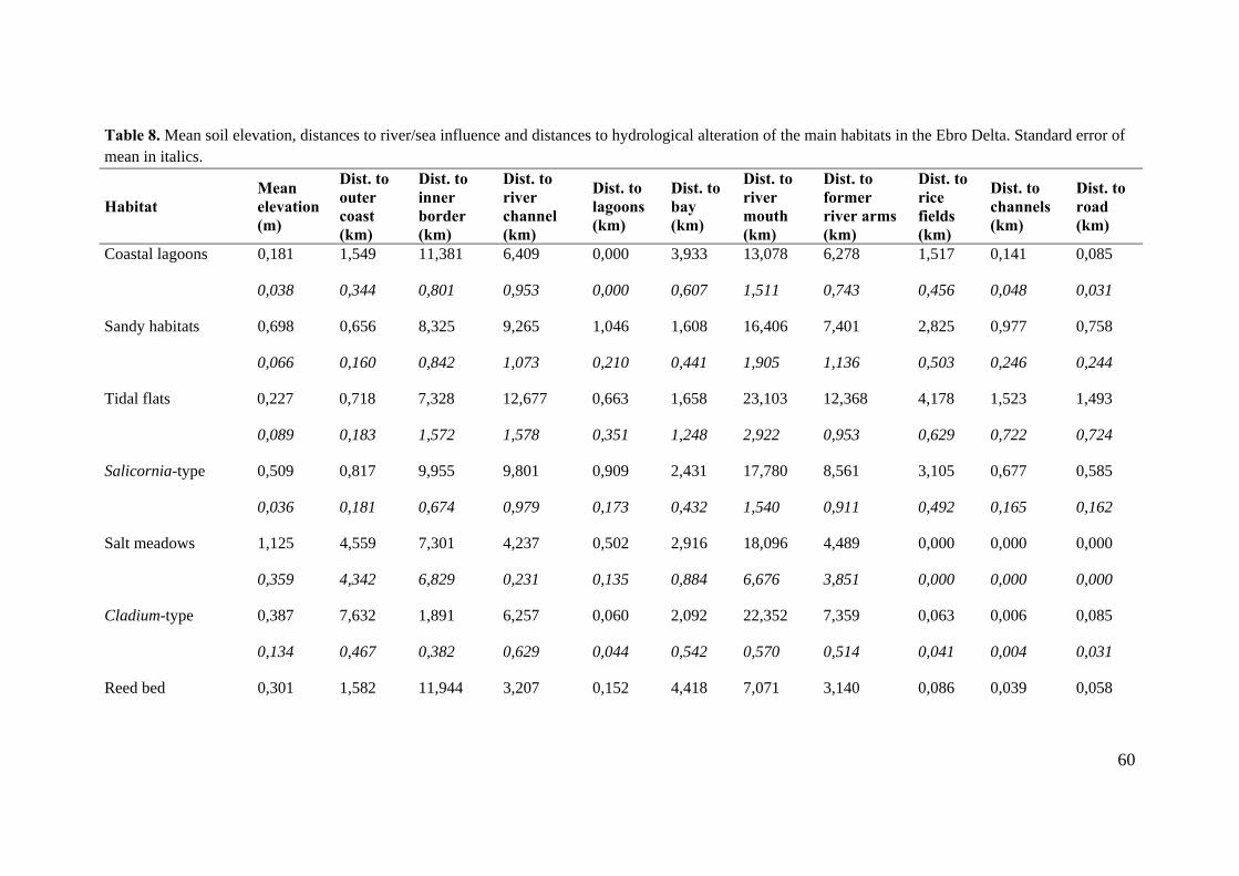
60
Table 8. Mean soil elevation, distances to river/sea influence and distances to hydrological alteration of the main habitats in the Ebro Delta. Standard error of mean in italics.
Habitat Mean elevation (m)
Dist. to outer coast (km)
Dist. to inner border (km)
Dist. to river channel (km)
Dist. to lagoons (km)
Dist. to bay (km)
Dist. to river mouth (km)
Dist. to former river arms (km)
Dist. to rice fields (km)
Dist. to channels (km)
Dist. to road (km)
Coastal lagoons 0,181 1,549 11,381 6,409 0,000 3,933 13,078 6,278 1,517 0,141 0,085
0,038 0,344 0,801 0,953 0,000 0,607 1,511 0,743 0,456 0,048 0,031
Sandy habitats 0,698 0,656 8,325 9,265 1,046 1,608 16,406 7,401 2,825 0,977 0,758
0,066 0,160 0,842 1,073 0,210 0,441 1,905 1,136 0,503 0,246 0,244
Tidal flats 0,227 0,718 7,328 12,677 0,663 1,658 23,103 12,368 4,178 1,523 1,493
0,089 0,183 1,572 1,578 0,351 1,248 2,922 0,953 0,629 0,722 0,724
Salicornia-type 0,509 0,817 9,955 9,801 0,909 2,431 17,780 8,561 3,105 0,677 0,585
0,036 0,181 0,674 0,979 0,173 0,432 1,540 0,911 0,492 0,165 0,162
Salt meadows 1,125 4,559 7,301 4,237 0,502 2,916 18,096 4,489 0,000 0,000 0,000
0,359 4,342 6,829 0,231 0,135 0,884 6,676 3,851 0,000 0,000 0,000
Cladium-type 0,387 7,632 1,891 6,257 0,060 2,092 22,352 7,359 0,063 0,006 0,085
0,134 0,467 0,382 0,629 0,044 0,542 0,570 0,514 0,041 0,004 0,031
Reed bed 0,301 1,582 11,944 3,207 0,152 4,418 7,071 3,140 0,086 0,039 0,058
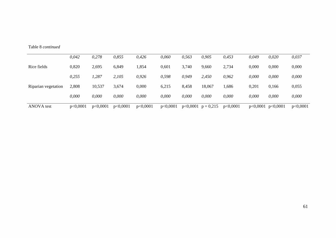
61
Table 8 continued
0,042 0,278 0,855 0,426 0,060 0,563 0,905 0,453 0,049 0,020 0,037
Rice fields 0,820 2,695 6,849 1,854 0,601 3,740 9,660 2,734 0,000 0,000 0,000
0,255 1,287 2,105 0,926 0,598 0,949 2,450 0,962 0,000 0,000 0,000
Riparian vegetation 2,808 10,537 3,674 0,000 6,215 8,458 18,067 1,686 0,201 0,166 0,055
0,000 0,000 0,000 0,000 0,000 0,000 0,000 0,000 0,000 0,000 0,000
ANOVA test p<0,0001 p<0,0001 p<0,0001 p<0,0001 p<0,0001 p<0,0001 p = 0,215 p<0,0001 p<0,0001 p<0,0001 p<0,0001
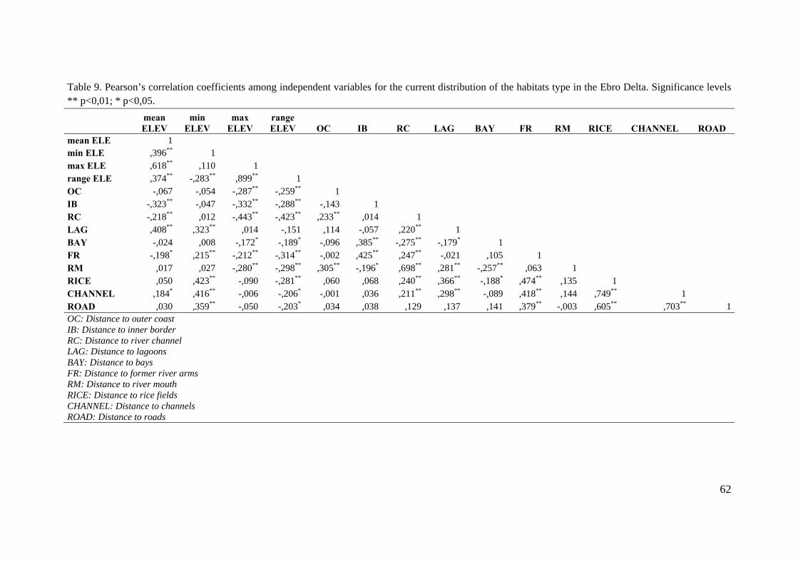
62
Table 9. Pearson’s correlation coefficients among independent variables for the current distribution of the habitats type in the Ebro Delta. Significance levels ** p<0,01; * p<0,05.
mean ELEV
min ELEV
max ELEV
range ELEV OC IB RC LAG BAY FR RM RICE CHANNEL ROAD
mean ELE 1 min ELE ,396** 1 max ELE ,618** ,110 1 range ELE ,374** -,283** ,899** 1 OC -,067 -,054 -,287** -,259** 1 IB -,323** -,047 -,332** -,288** -,143 1 RC -,218** ,012 -,443** -,423** ,233** ,014 1 LAG ,408** ,323** ,014 -,151 ,114 -,057 ,220** 1 BAY -,024 ,008 -,172* -,189* -,096 ,385** -,275** -,179* 1 FR -,198* ,215** -,212** -,314** -,002 ,425** ,247** -,021 ,105 1 RM ,017 ,027 -,280** -,298** ,305** -,196* ,698** ,281** -,257** ,063 1 RICE ,050 ,423** -,090 -,281** ,060 ,068 ,240** ,366** -,188* ,474** ,135 1 CHANNEL ,184* ,416** -,006 -,206* -,001 ,036 ,211** ,298** -,089 ,418** ,144 ,749** 1 ROAD ,030 ,359** -,050 -,203* ,034 ,038 ,129 ,137 ,141 ,379** -,003 ,605** ,703** 1 OC: Distance to outer coast IB: Distance to inner border RC: Distance to river channel LAG: Distance to lagoons BAY: Distance to bays FR: Distance to former river arms RM: Distance to river mouth RICE: Distance to rice fields CHANNEL: Distance to channels ROAD: Distance to roads
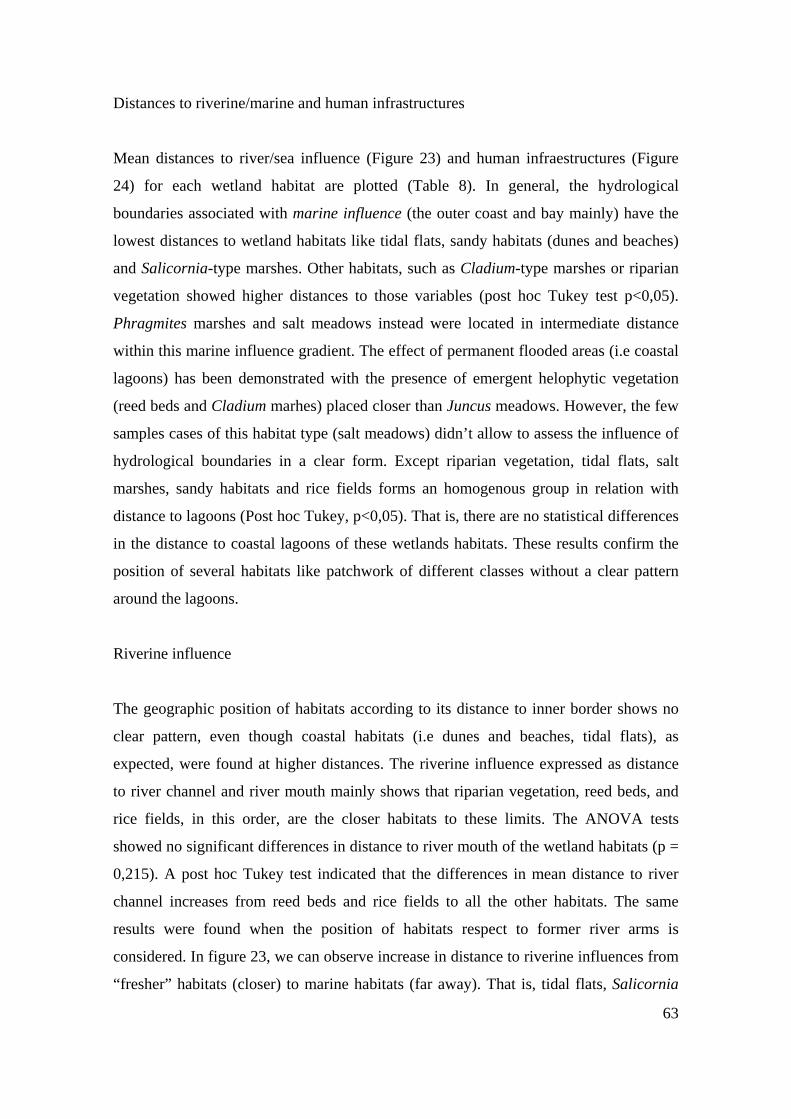
63
Distances to riverine/marine and human infrastructures
Mean distances to river/sea influence (Figure 23) and human infraestructures (Figure
24) for each wetland habitat are plotted (Table 8). In general, the hydrological
boundaries associated with marine influence (the outer coast and bay mainly) have the
lowest distances to wetland habitats like tidal flats, sandy habitats (dunes and beaches)
and Salicornia-type marshes. Other habitats, such as Cladium-type marshes or riparian
vegetation showed higher distances to those variables (post hoc Tukey test p<0,05).
Phragmites marshes and salt meadows instead were located in intermediate distance
within this marine influence gradient. The effect of permanent flooded areas (i.e coastal
lagoons) has been demonstrated with the presence of emergent helophytic vegetation
(reed beds and Cladium marhes) placed closer than Juncus meadows. However, the few
samples cases of this habitat type (salt meadows) didn’t allow to assess the influence of
hydrological boundaries in a clear form. Except riparian vegetation, tidal flats, salt
marshes, sandy habitats and rice fields forms an homogenous group in relation with
distance to lagoons (Post hoc Tukey, p<0,05). That is, there are no statistical differences
in the distance to coastal lagoons of these wetlands habitats. These results confirm the
position of several habitats like patchwork of different classes without a clear pattern
around the lagoons.
Riverine influence
The geographic position of habitats according to its distance to inner border shows no
clear pattern, even though coastal habitats (i.e dunes and beaches, tidal flats), as
expected, were found at higher distances. The riverine influence expressed as distance
to river channel and river mouth mainly shows that riparian vegetation, reed beds, and
rice fields, in this order, are the closer habitats to these limits. The ANOVA tests
showed no significant differences in distance to river mouth of the wetland habitats (p =
0,215). A post hoc Tukey test indicated that the differences in mean distance to river
channel increases from reed beds and rice fields to all the other habitats. The same
results were found when the position of habitats respect to former river arms is
considered. In figure 23, we can observe increase in distance to riverine influences from
“fresher” habitats (closer) to marine habitats (far away). That is, tidal flats, Salicornia
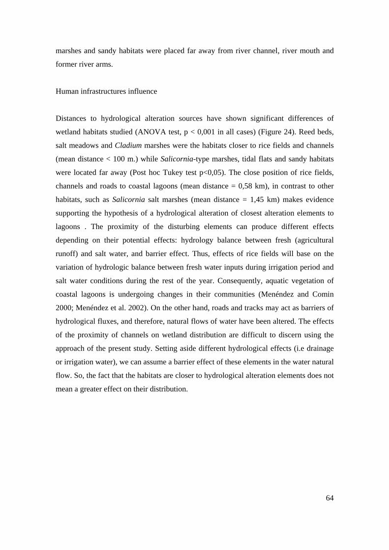
64
marshes and sandy habitats were placed far away from river channel, river mouth and
former river arms.
Human infrastructures influence
Distances to hydrological alteration sources have shown significant differences of
wetland habitats studied (ANOVA test, p < 0,001 in all cases) (Figure 24). Reed beds,
salt meadows and Cladium marshes were the habitats closer to rice fields and channels
(mean distance < 100 m.) while Salicornia-type marshes, tidal flats and sandy habitats
were located far away (Post hoc Tukey test p<0,05). The close position of rice fields,
channels and roads to coastal lagoons (mean distance = 0,58 km), in contrast to other
habitats, such as Salicornia salt marshes (mean distance = 1,45 km) makes evidence
supporting the hypothesis of a hydrological alteration of closest alteration elements to
lagoons . The proximity of the disturbing elements can produce different effects
depending on their potential effects: hydrology balance between fresh (agricultural
runoff) and salt water, and barrier effect. Thus, effects of rice fields will base on the
variation of hydrologic balance between fresh water inputs during irrigation period and
salt water conditions during the rest of the year. Consequently, aquatic vegetation of
coastal lagoons is undergoing changes in their communities (Menéndez and Comin
2000; Menéndez et al. 2002). On the other hand, roads and tracks may act as barriers of
hydrological fluxes, and therefore, natural flows of water have been altered. The effects
of the proximity of channels on wetland distribution are difficult to discern using the
approach of the present study. Setting aside different hydrological effects (i.e drainage
or irrigation water), we can assume a barrier effect of these elements in the water natural
flow. So, the fact that the habitats are closer to hydrological alteration elements does not
mean a greater effect on their distribution.
65
0 2 4 6 8 10 12
Sandy habitatsTidal flats
Salicornia-typeCoastal lagoons
Reed bedRice fields
Salt meadowsCladium-type
Riparian vegetation
Distance to outer coast (km)
0 2 4 6 8 10 12 14 16
Rice fields
Riparian vegetation
Cladium-type
Reed bed
Salicornia-type
Tidal flats
Coastal lagoons
Sandy habitats
Salt meadows
Distance to inner border (km)
0 1 2 3 4 5 6 7 8 9
Sandy habitats
Tidal flats
Cladium-type
Salicornia-type
Salt meadows
Rice fields
Coastal lagoons
Reed bed
Riparian vegetation
Distance to bay (km)
0 1 2 3 4 5 6 7
Coastal lagoons
Cladium-type
Reed bed
Salt meadows
Rice fields
Tidal flats
Salicornia-type
Sandy habitats
Riparian vegetation
Distance to lagoons (km)
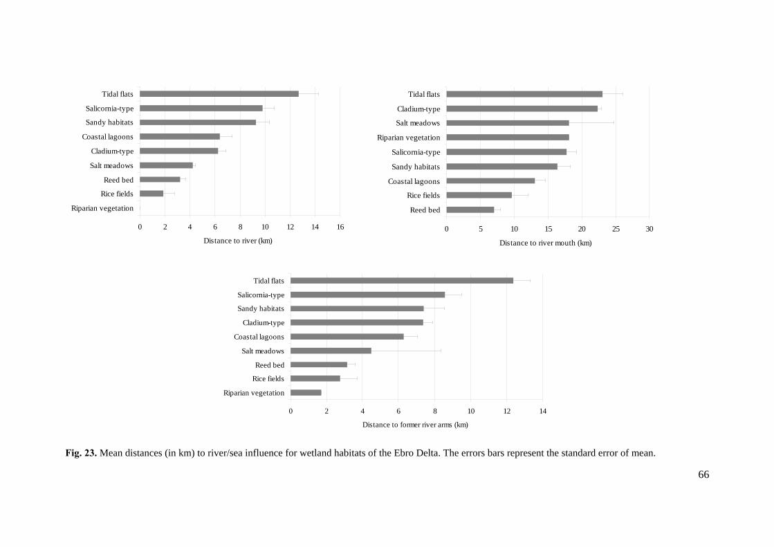
66
0 2 4 6 8 10 12 14 16
Riparian vegetation
Rice fields
Reed bed
Salt meadows
Cladium-type
Coastal lagoons
Sandy habitats
Salicornia-type
Tidal flats
Distance to river (km)
0 5 10 15 20 25 30
Reed bed
Rice fields
Coastal lagoons
Sandy habitats
Salicornia-type
Riparian vegetation
Salt meadows
Cladium-type
Tidal flats
Distance to river mouth (km)
0 2 4 6 8 10 12 14
Riparian vegetation
Rice fields
Reed bed
Salt meadows
Coastal lagoons
Cladium-type
Sandy habitats
Salicornia-type
Tidal flats
Distance to former river arms (km)
Fig. 23. Mean distances (in km) to river/sea influence for wetland habitats of the Ebro Delta. The errors bars represent the standard error of mean.
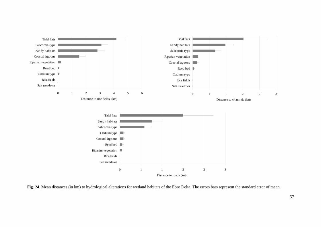
67
0 1 2 3 4 5 6
Salt meadows
Rice fields
Cladium-type
Reed bed
Riparian vegetation
Coastal lagoons
Sandy habitats
Salicornia-type
Tidal flats
Distance to rice fields (km)
0 1 1 2 2 3
Salt meadows
Rice fields
Cladium-type
Reed bed
Coastal lagoons
Riparian vegetation
Salicornia-type
Sandy habitats
Tidal flats
Distance to channels (km)
0 1 1 2 2 3
Salt meadows
Rice fields
Riparian vegetation
Reed bed
Coastal lagoons
Cladium-type
Salicornia-type
Sandy habitats
Tidal flats
Distance to roads (km)
Fig. 24. Mean distances (in km) to hydrological alterations for wetland habitats of the Ebro Delta. The errors bars represent the standard error of mean.
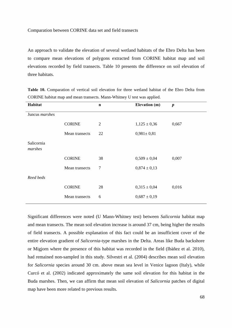
68
Comparation between CORINE data set and field transects
An approach to validate the elevation of several wetland habitats of the Ebro Delta has been
to compare mean elevations of polygons extracted from CORINE habitat map and soil
elevations recorded by field transects. Table 10 presents the difference on soil elevation of
three habitats.
Table 10. Comparation of vertical soil elevation for three wetland habitat of the Ebro Delta from
CORINE habitat map and mean transects. Mann-Whitney U test was applied.
Habitat n Elevation (m) p
Juncus marshes
CORINE 2 1,125 ± 0,36 0,667
Mean transects 22 0,981± 0,81
Salicornia marshes
CORINE 38 0,509 ± 0,04 0,007
Mean transects 7 0,874 ± 0,13
Reed beds
CORINE 28 0,315 ± 0,04 0,016
Mean transects 6 0,687 ± 0,19
Significant differences were noted (U Mann-Whitney test) between Salicornia habitat map
and mean transects. The mean soil elevation increase is around 37 cm, being higher the results
of field transects. A possible explanation of this fact could be an insufficient cover of the
entire elevation gradient of Salicornia-type marshes in the Delta. Areas like Buda backshore
or Migjorn where the presence of this habitat was recorded in the field (Ibàñez et al. 2010),
had remained non-sampled in this study. Silvestri et al. (2004) describes mean soil elevation
for Salicornia species around 30 cm. above mean sea level in Venice lagoon (Italy), while
Curcó et al. (2002) indicated approximately the same soil elevation for this habitat in the
Buda marshes. Then, we can affirm that mean soil elevation of Salicornia patches of digital
map have been more related to previous results.
69
Habitat of reed beds showed also significant differences between the patches of habitat map
and field transects (U Mann-Whitney test). Mean soil elevation was twice in the field samples
of Phragmites marshes. The effect of unsampled areas of reed beds located in the edge of the
most lagoons (i.e. lower vertical elevations) might be a plausible explanation of this
difference. Reviewing literature we find many authors concluding that elevation is a primary
forcing factor on Phragmites distribution around the fresh water shorelines coupled with soil
organic matter (Welch et al. 2006). Lensen et al. (2000) reported a mean elevation of
Phragmites relevés around 10 cm below sea level water, demonstrating its preference for
flooded soils. Therefore, our results were not in concordance with their findings.
The mean soil elevation of salt meadow showed no significant differences between digital
map and field transects (U Mann-Whitney test). Despite the low number of polygons analyzed
by CORINE land cover was low (n=2), these can be considered as representative of the
Juncus marshes elevation of the Delta. The range elevation of Juncus presence in field
transects (1,75m.) could be associated with its natural ranges occupying transitional stages
between areas with succulent halophytes (e.g. Salicornia vegetation) and habitats lacking
halophytic vegetation.
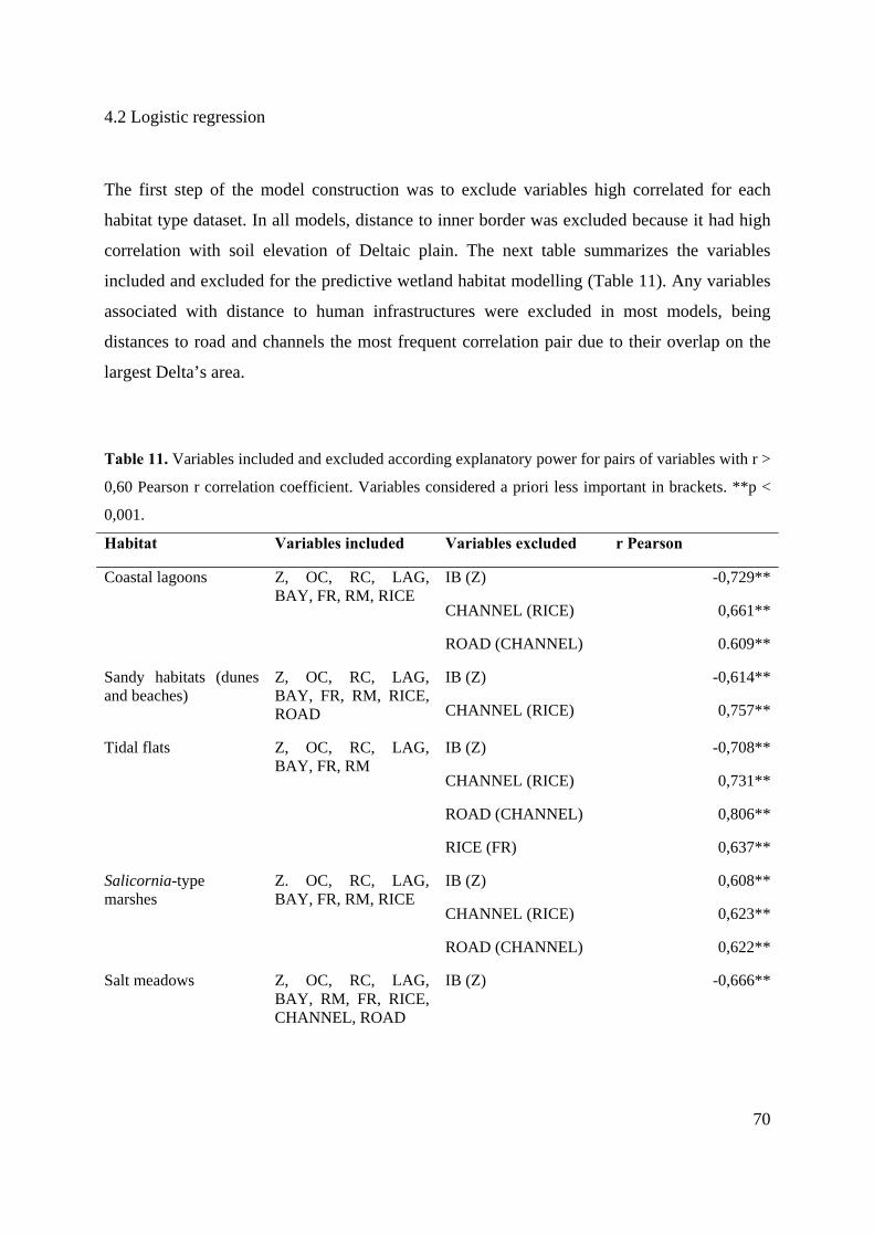
70
4.2 Logistic regression
The first step of the model construction was to exclude variables high correlated for each
habitat type dataset. In all models, distance to inner border was excluded because it had high
correlation with soil elevation of Deltaic plain. The next table summarizes the variables
included and excluded for the predictive wetland habitat modelling (Table 11). Any variables
associated with distance to human infrastructures were excluded in most models, being
distances to road and channels the most frequent correlation pair due to their overlap on the
largest Delta’s area.
Table 11. Variables included and excluded according explanatory power for pairs of variables with r >
0,60 Pearson r correlation coefficient. Variables considered a priori less important in brackets. **p <
0,001.
Habitat Variables included Variables excluded r Pearson
Coastal lagoons Z, OC, RC, LAG, BAY, FR, RM, RICE
IB (Z)
CHANNEL (RICE)
ROAD (CHANNEL)
-0,729**
0,661**
0.609**
Sandy habitats (dunes and beaches)
Z, OC, RC, LAG, BAY, FR, RM, RICE, ROAD
IB (Z)
CHANNEL (RICE)
-0,614**
0,757**
Tidal flats Z, OC, RC, LAG, BAY, FR, RM
IB (Z)
CHANNEL (RICE)
ROAD (CHANNEL)
RICE (FR)
-0,708**
0,731**
0,806**
0,637**
Salicornia-type marshes
Z. OC, RC, LAG, BAY, FR, RM, RICE
IB (Z)
CHANNEL (RICE)
ROAD (CHANNEL)
0,608**
0,623**
0,622**
Salt meadows Z, OC, RC, LAG, BAY, RM, FR, RICE, CHANNEL, ROAD
IB (Z) -0,666**
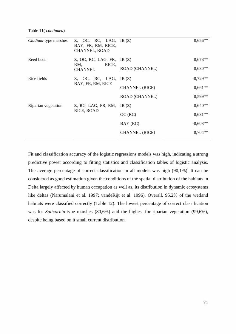
71
Table 11( continued)
Cladium-type marshes Z, OC, RC, LAG, BAY, FR, RM, RICE, CHANNEL, ROAD
IB (Z) 0,656**
Reed beds Z, OC, RC, LAG, FR, RM, RICE, CHANNEL
IB (Z)
ROAD (CHANNEL)
-0,678**
0,630**
Rice fields Z, OC, RC, LAG, BAY, FR, RM, RICE
IB (Z)
CHANNEL (RICE)
ROAD (CHANNEL)
-0,729**
0,661**
0,599**
Riparian vegetation Z, RC, LAG, FR, RM, RICE, ROAD
IB (Z)
OC (RC)
BAY (RC)
CHANNEL (RICE)
-0,640**
0,631**
-0,603**
0,704**
Fit and classification accuracy of the logistic regressions models was high, indicating a strong
predictive power according to fitting statistics and classification tables of logistic analysis.
The average percentage of correct classification in all models was high (90,1%). It can be
considered as good estimation given the conditions of the spatial distribution of the habitats in
Delta largely affected by human occupation as well as, its distribution in dynamic ecosystems
like deltas (Narumalani et al. 1997; vandeRijt et al. 1996). Overall, 95,2% of the wetland
habitats were classified correctly (Table 12). The lowest percentage of correct classification
was for Salicornia-type marshes (80,6%) and the highest for riparian vegetation (99,6%),
despite being based on it small current distribution.
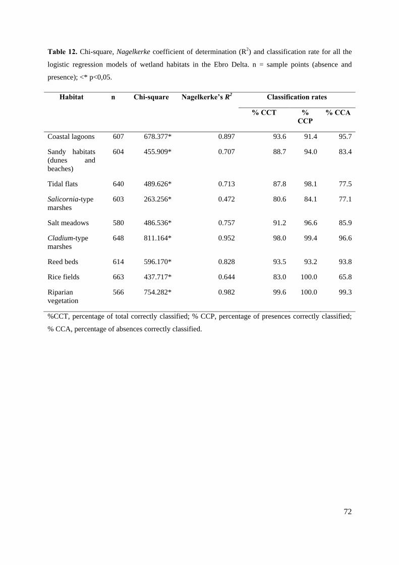
72
Table 12. Chi-square, Nagelkerke coefficient of determination (R2) and classification rate for all the
logistic regression models of wetland habitats in the Ebro Delta. n = sample points (absence and
presence); <* p<0,05.
Habitat n Chi-square Nagelkerke’s R2 Classification rates
% CCT % CCP
% CCA
Coastal lagoons 607 678.377* 0.897 93.6 91.4 95.7
Sandy habitats (dunes and beaches)
604 455.909* 0.707 88.7 94.0 83.4
Tidal flats 640 489.626* 0.713 87.8 98.1 77.5
Salicornia-type marshes
603 263.256* 0.472 80.6 84.1 77.1
Salt meadows 580 486.536* 0.757 91.2 96.6 85.9
Cladium-type marshes
648 811.164* 0.952 98.0 99.4 96.6
Reed beds 614 596.170* 0.828 93.5 93.2 93.8
Rice fields 663 437.717* 0.644 83.0 100.0 65.8
Riparian vegetation
566 754.282* 0.982 99.6 100.0 99.3
%CCT, percentage of total correctly classified; % CCP, percentage of presences correctly classified;
% CCA, percentage of absences correctly classified.
73
The best fitting logistic models includes different independent variables for the wetland
habitats distribution. The coefficients and statistics for the terrain environment variables are
listed in the table 13. In terms of marine influence, the most frequent variables in the models
are distance to outer coast and distance to lagoons, while distance to former river arms and
river channel have been the most significant variables describing riverine influence. The soil
elevation was present as significant variable in the distribution of 4 wetland habitats: sandy
habitats, Cladium marshes, rice fields and riparian vegetation. Our results indicate that
distance to rice fields has been the most significant anthropogenic variable in 5 out of 11
wetland habitats.
In general, the variables describing the distribution of marine influenced habitats in the
logistic regression models, such as coastal lagoons, dunes and beaches, tidal flats and
Salicornia salt marshes were not considerably different from those describing Cladium-type
marshes, reed beds and riparian forests (that receives less marine influence). The models
showed that coastal habitats occurrence was significantly related to distance to outer coast in
all cases. This variable appeared also in the predictive model of helophytic habitats (Cladium
and Phragmites marshes). The effect of former river course position on wetland habitat
distribution was significant in the most habitats, which can be indirectly linked with soil
elevation change (former lévées have more elevation). Distance to river channel has
influenced the occurrence of salt meadows and riparian vegetation. Among distance to
anthropogenic elements (roads and channels) and artificial habitats (rice fields), the last
variable was significantly related to coastal lagoons and several marshes (Salicornia-type,
reed beds and Cladium-type), thus demonstrating the proximity effect in these habitats. In the
next section, we describe the results of logistic models for each habitat type and we discuss its
accuracy.
Coastal lagoons
The analysis of logistic regression coefficients shows that the variables distance to outer
coast, lagoons, former river arms and rice fields are significant in predicting the probability of
74
coastal lagoons occurrence. Our results for costal lagoons model cover an area under the
curve of 0.986, which represent a very good predictive capacity (Figure 25).
Fig. 25. Receiver operating characteristic (ROC) curve for costal lagoons logistic model. The area
under the curve is 0.986.
According to the full model, coastal lagoon occurrence was not influenced by soil elevation
despite being a key terrain variable determining its distribution, since they occupy areas
permanently under sea level (Curcó et al. 1995). A more specific analysis taking into account
soil elevation as the sole predictor in the logistic regression revealed that topography was a
significant variable in the probability of coastal lagoons presence (Wald’s = 75,099, p<0,001).
The reliability of the Digital Elevation Model of Ebro Delta must be taken cautiously, in this
case, since the method for obtaining the elevation data (LIDAR) does not work properly
under water.
75
Sandy habitats (dunes and beaches)
The variables that describe the distribution of dunes and beaches in the Ebro Delta are
diverse, so they respond to different factors. Regarding to variables that respond to marine
influence, distance to outer coast should have a meaningful relation to its distribution since
this natural geographic position. Sand materials are mobilized from the river front that is
exposed to marine action, being deposited in coastal areas where several conditions are met
(sedimentary balance, winds and coast orientation mainly). The influence of elevation was
significant and plays an important role in discriminating the presence of this habitat.
However, the sandy habitat classification adopted in this study (dunes and beaches), does not
consider differences in soil elevation between several dunes systems (i.e shifting, fixed)
(Korakis and Gerasimidis 2006) have not been assessed. Overall, the AUC in the model that
performs the distribution of sandy habitats covers an area of 0,930, which represent very good
model accuracy (Figure 26).
Fig. 26. Receiver operating characteristic (ROC) curve for sandy habitats logistic model. The area
under the curve is 0.930.
76
Tidal flats
The variables included in the model seem to be related to a greater extent with the river
influence, given that distances to river mouth, river channel and ancient river courses were
significant in their distribution and only distance to coast was selected among “marine”
variables. Proximity to sea plays an important role in their occurrence probability, while soil
elevation was not selected by the logistic regression model. According to its distribution,
mainly in la Banya spit at south end of Delta, the elevation coupled with periodically drying-
flooding conditions allows its establishment (Martínez-Alonso et al. 2004; Mir et al. 2000).
As we expected, logistic regression carried out between elevation as terrain predictor and
occurrence of tidal flats as dependent variable has yielded significant dependence between
presence of the habitat and elevation (Wald’s = 63,488, p<0,001). This model classified
accurately 70,3% of cases through soil elevation. For the full logistic model, the AUC was
high (0,914) that show a good accuracy of the predictive distribution of the tidal flats in the
Ebro Delta (Figure).
Fig. 27. Receiver operating characteristic (ROC) curve for tidal flats logistic model. The area under the
curve is 0.914.
77
Salicornia-type marshes
The variables selected by regression logistic model have described the distribution of salt
marshes according to distance to outer coast and lagoons. The riverine influence on these
habitats appears reflected by the inclusion in the model of the relative position of the river
mouth. Distance to rice fields was also a significant variable describing the distribution of
Salicornia-type marshes, showing the importance of these artificial habitats on occurrence
probability of this halophilous vegetation. Soil elevation should be a key variable in
discriminating the presence of Salicornia marshes in the Delta, but in the logistic regression it
was not reflected. According to Maldonado (1972) and reviewed by Curcó et al. (1995),
elevation areas between 0 and 0,4 metres above mean sea level, are exposed to marine floods.
So, topography plays a major role in the distribution of salt marshes in Deltaic plain. Overall,
according to the full model, the accuracy of predictive distribution of Salicornia marshes was
high, with an AUC of 0,855.
Fig. 28. Receiver operating characteristic (ROC) curve for Salicornia-type marshes logistic model. The
area under the curve is 0,855.
78
Salt meadows
The logistic regression for this habitat allows the identification of significant variables that
describe its distribution: distance to bay, distance to river channel, distance to former river
arms and distance to channels. These results suggest that the occurrence of salt meadows in
the Ebro Delta can be explained to a reasonable degree by the combination of several
distances (AUC = 0,955). However, due to the high degree of surface loss from their natural
areas, the current distribution of these habitats is little representative and therefore the
presence points ( (is clearly a limitant factor. Soil elevation is certainly a major factor of salt
meadow presence as reported by the literature (Moffett et al. 2010; Silvestri et al. 2005), as
well as soil salinity content (Álvarez-Rogel et al. 2007). Then, we expect that this habitat type
could form a transitional stage between exclusive halophytic vegetation (i.e coastal lagoon-
salt marsh complex) and areas less influenced by sea water and more influenced by the fresh
water near the fluvial levees (Curcó et al. 1995). According to our results (see current
distribution of wetland habitats section) soil elevation of Juncus habitat (salt meadows)
should range between 0,4 and 2,3m. Nowadays, this elevation range is occupied by the rice
fields and other crops, as well as several human infrastructures. Bockelmann et al. (2002)
used logistic regression to predict plant zonation in German intertidal salt marshes and they
find that inundation frequency explain approximately twice of the variance than soil
elevation.
Cladium-type marshes
The analysis of logistic regression coefficients shows that soil elevation, distances to outer
coast, river channel, former river arms and rice fields are significant in predicting the
probability of Cladium marsh occurrence. The predictive capacity of the model was very high
(AUC = 0,994). According to Curcó (2001), this habitat finds its original area in the natural
wells and some lagoons that receive a significant fresh groundwater supply. These natural
conditions are present near the inner border of the Deltaic plain as a result of inflows of
freshwater that come from the ascension of freatic waters due to low permeability of deltaic
79
sediments. A binary logistic regression was carried out to investigate the effect of distance to
inner border and probability of occurrence of Cladium-type marshes. Results show that most
Cladium habitat have occurred near the inner border and that the probability of its presence
depends on distance to the inner border (Wald’s = 135,546, p<0,000)(Figure 29).
Nevertheless distance to riverine influences plays an important role in the distribution of these
habitats; it seems that peat materials distribution could be also a determinant factor on their
occurrence (Maldonado 1972). Since the beginning of rice cultivation, the potential area of
this habitat has been occupied by rice fields and other crops. Although the model shows good
classification rates, this habitat type is considered to be altered since its probability of
occurrence depends also on the distance to rice fields and roads.
Fig. 29. Relationship between presence of Cladium-type marshes in the Ebro Delta with distance to
inner border. The crosses are known Cladium samples (0, absent; 1, present) and the circles are
occurrence probability fitted with logistic regression.
80
Reed beds
The variables describing the distribution of reed beds in the logistic regression model were in
contrast with those describing the other helophytic habitat of the Delta (Cladium marshes).
The preference of Phragmites for brackish waters has been shown by the importance of
distance to the lagoons and bays for describing, in part, the occurrence of this habitat. The
effect of hydrological changes, associated to drainage waters from the rice fields, has led to
the occupation of these habitats in the perimeter of most lagoons and some inner parts of the
bays. In addition, the probability of presence of reed beds was dependent on distance to
hydrological alteration sources (i.e rice fields and channels). The high accuracy of the
predictive model for Phragmites marshes (AUC = 0,974) does not implies a correct ecological
interpretation of its distribution due to the above commented factors. In contrast, Phragmites
marshes present in the Garxal area are reliable brackish marsh, since the lagoon is directly
influenced by the river discharge (Ibàñez et al. 2010).
Fig. 30. Receiver operating characteristic (ROC) curve for reed beds logistic model. The area under the
curve is 0,974.
81
Riparian vegetation
This habitat presented a good model accuracy, despite having low representation in terms of
extension in the Ebro Delta. As expected, elevation and distance to river channel explained a
reasonable occurrence of the riparian vegetation in the Delta, and distance to lagoons was also
a significant variable. This habitat type occupied the fluvial lévées that are located 3-4 metres
above mean sea level and its elevation gradually decreased to the sea, but nowadays its
distribution has been drastically reduced (Curcó et al. 1995). The variable relating presence of
riparian vegetation in former river arms position was not selected by the logistic model
although these structures have, in part, higher soil elevation (Riet de Zaida, 1,7m; Riet dels
Muntells, 1,4 m) and because it was removed (Ibànez et al. 1997). Shoutis et al. (2010) used a
predictive model (Generalized Liniar Models, GLM) to generate riparian-environment
relationships using the elevation above the channel as a single predictor. The authors found
thresholds of 50% of probability to find riparian forests between 1,1 m and 1,75 m. In our
results, the area under the curve corresponding to the present logistic model is 0,966, which
implies a good predictive capacity.
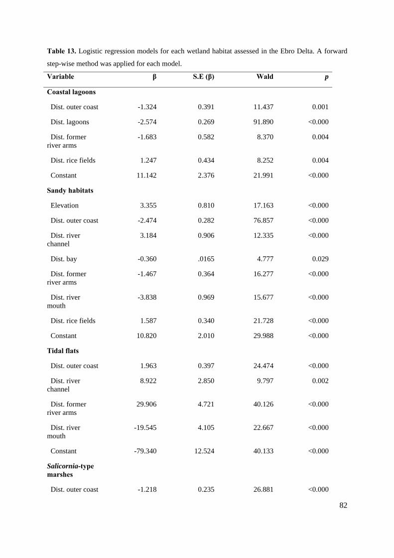
82
Table 13. Logistic regression models for each wetland habitat assessed in the Ebro Delta. A forward
step-wise method was applied for each model.
Variable β S.E (β) Wald p
Coastal lagoons
Dist. outer coast -1.324 0.391 11.437 0.001
Dist. lagoons -2.574 0.269 91.890 <0.000
Dist. former river arms
-1.683 0.582 8.370 0.004
Dist. rice fields 1.247 0.434 8.252 0.004
Constant 11.142 2.376 21.991 <0.000
Sandy habitats
Elevation 3.355 0.810 17.163 <0.000
Dist. outer coast -2.474 0.282 76.857 <0.000
Dist. river channel
3.184 0.906 12.335 <0.000
Dist. bay -0.360 .0165 4.777 0.029
Dist. former river arms
-1.467 0.364 16.277 <0.000
Dist. river mouth
-3.838 0.969 15.677 <0.000
Dist. rice fields 1.587 0.340 21.728 <0.000
Constant 10.820 2.010 29.988 <0.000
Tidal flats
Dist. outer coast 1.963 0.397 24.474 <0.000
Dist. river channel
8.922 2.850 9.797 0.002
Dist. former river arms
29.906 4.721 40.126 <0.000
Dist. river mouth
-19.545 4.105 22.667 <0.000
Constant -79.340 12.524 40.133 <0.000
Salicornia-type marshes
Dist. outer coast -1.218 0.235 26.881 <0.000
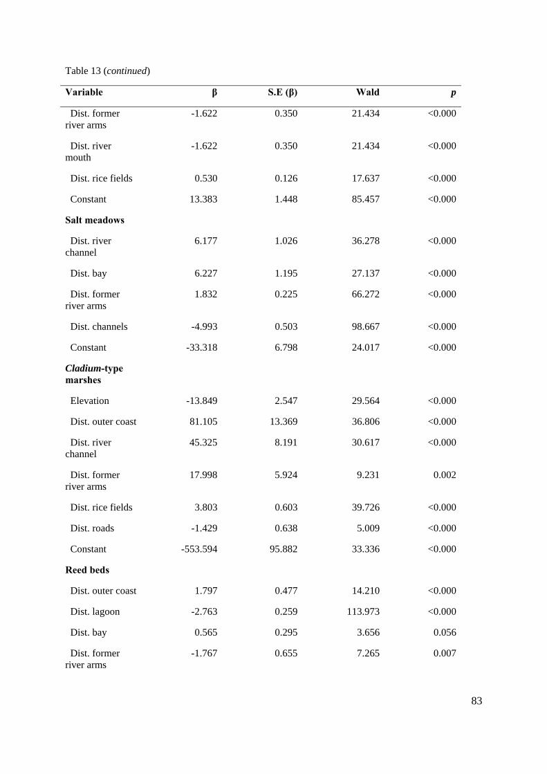
83
Table 13 (continued)
Variable β S.E (β) Wald p
Dist. former river arms
-1.622 0.350 21.434 <0.000
Dist. river mouth
-1.622 0.350 21.434 <0.000
Dist. rice fields 0.530 0.126 17.637 <0.000
Constant 13.383 1.448 85.457 <0.000
Salt meadows
Dist. river channel
6.177 1.026 36.278 <0.000
Dist. bay 6.227 1.195 27.137 <0.000
Dist. former river arms
1.832 0.225 66.272 <0.000
Dist. channels -4.993 0.503 98.667 <0.000
Constant -33.318 6.798 24.017 <0.000
Cladium-type marshes
Elevation -13.849 2.547 29.564 <0.000
Dist. outer coast 81.105 13.369 36.806 <0.000
Dist. river channel
45.325 8.191 30.617 <0.000
Dist. former river arms
17.998 5.924 9.231 0.002
Dist. rice fields 3.803 0.603 39.726 <0.000
Dist. roads -1.429 0.638 5.009 <0.000
Constant -553.594 95.882 33.336 <0.000
Reed beds
Dist. outer coast 1.797 0.477 14.210 <0.000
Dist. lagoon -2.763 0.259 113.973 <0.000
Dist. bay 0.565 0.295 3.656 0.056
Dist. former river arms
-1.767 0.655 7.265 0.007
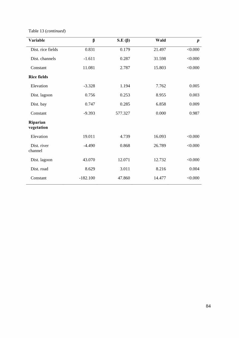
84
Table 13 (continued)
Variable β S.E (β) Wald p
Dist. rice fields 0.831 0.179 21.497 <0.000
Dist. channels -1.611 0.287 31.598 <0.000
Constant 11.081 2.787 15.803 <0.000
Rice fields
Elevation -3.328 1.194 7.762 0.005
Dist. lagoon 0.756 0.253 8.955 0.003
Dist. bay 0.747 0.285 6.858 0.009
Constant -9.393 577.327 0.000 0.987
Riparian vegetation
Elevation 19.011 4.739 16.093 <0.000
Dist. river channel
-4.490 0.868 26.789 <0.000
Dist. lagoon 43.070 12.071 12.732 <0.000
Dist. road 8.629 3.011 8.216 0.004
Constant -182.100 47.860 14.477 <0.000
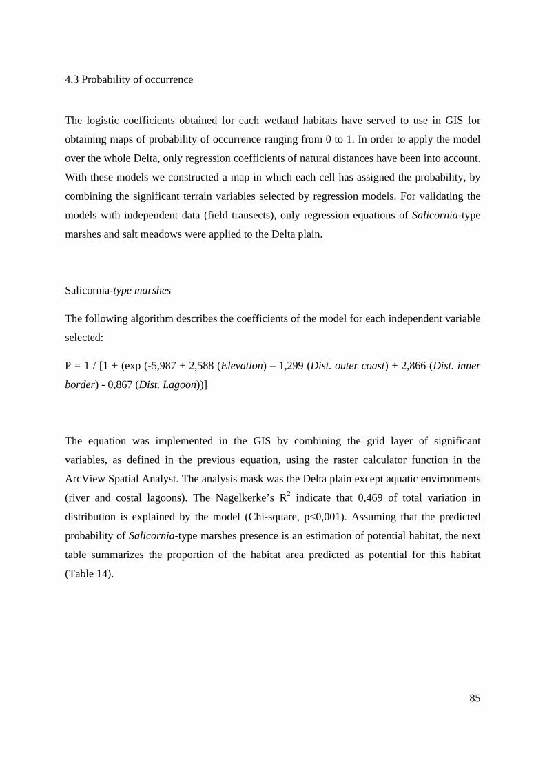
85
4.3 Probability of occurrence
The logistic coefficients obtained for each wetland habitats have served to use in GIS for
obtaining maps of probability of occurrence ranging from 0 to 1. In order to apply the model
over the whole Delta, only regression coefficients of natural distances have been into account.
With these models we constructed a map in which each cell has assigned the probability, by
combining the significant terrain variables selected by regression models. For validating the
models with independent data (field transects), only regression equations of Salicornia-type
marshes and salt meadows were applied to the Delta plain.
Salicornia-type marshes
The following algorithm describes the coefficients of the model for each independent variable
selected:
P = 1 / [1 + (exp (-5,987 + 2,588 (Elevation) – 1,299 (Dist. outer coast) + 2,866 (Dist. inner
border) - 0,867 (Dist. Lagoon))]
The equation was implemented in the GIS by combining the grid layer of significant
variables, as defined in the previous equation, using the raster calculator function in the
ArcView Spatial Analyst. The analysis mask was the Delta plain except aquatic environments
(river and costal lagoons). The Nagelkerke’s R2 indicate that 0,469 of total variation in
distribution is explained by the model (Chi-square, p<0,001). Assuming that the predicted
probability of Salicornia-type marshes presence is an estimation of potential habitat, the next
table summarizes the proportion of the habitat area predicted as potential for this habitat
(Table 14).
86
Table 14. Proportion of the current distribution predicted as potential habitat for Salicornia-type
marshes in the Ebro Delta, as guided by probability of habitat occurrence. Percentage of total Ebro
Delta did not include river and coastal lagoons surface.
Probability of occurrence
Area (km2)
Percentage of total Salicornia area
Percentage of total natural habitats
Percentage of total Ebro Delta
0,1 ,098 0,94 0,16 40,550,2 ,102 0,97 0,16 18,140,3 ,390 3,72 0,63 13,700,4 ,493 4,70 0,79 8,400,5 1,035 9,87 1,66 5,760,6 ,062 0,59 0,10 4,000,7 1,477 14,08 2,37 2,930,8 3,800 36,24 6,09 2,520,9 2,373 22,62 3,80 2,49
1 ,657 6,27 1,05 1,51
Overlapping the probability model over the habitat map of presence of Salicornia marshes
from CORINE land cover, we validate the current distribution of the habitat for each class of
predicted probability. Assuming a cut-off level of 0,50 probability value, nearly 10% of total
area of Salicornia-type marshes (1,1 out 10,50 km2) was in zones of lower than 50%
probability. Approximately 90% of total area of the habitat (9,40 out 10,50 km2) was in
regions of greater than 50% probability presence, so it is become dominant. Then we can
conclude that the current distribution of Salicornia habitat is located in higher predicted areas
by the model.
The habitat predictive map for the whole Delta was assessed for 31.826.930 grid cells
(resolution: 1m). The prediction for near 40 % of the total area of the Ebro Delta was 0,1 of
probability occurrence for Salicornia salt marshes (areas outside marine influence mainly),
while near 7% of Delta was suitable at more than 0,8 of probability occurrence.
Assuming predicted area as potential habitat for Salicornia-type marshes, 9,40 km2 (15,1%) of
total natural habitats area will be occupied by the wetland with more than 50% probability
and 6,83 km2 (10,9%) with more than 80% probability (Figure 31).
87
LegendSalicornia marshes (CLC)Natural habitats
Probability of occurrenceHigh : 1,0
Low : 0,00 5 102,5
km.
´
Fig. 31. Predicted distribution of Salicornia-type marshes based on regression coefficients coupled
with current distribution of the habitat based on CORINE land cover (CLC).
In order to validate the predicted presence of the habitat along elevation gradient, areas with
different cut-off of probability were compared with results of elevation transects. The next
figure shows the mean soil elevation of Salicornia marshes for classes of probability
occurrence (Figure). Mean soil elevation of the habitat predicted by regression model is 0,48
± 0,03 m. and 0,84 ± 0,12 m. for independent data (field transects). An independent T test was
performed to compare samples of Salicornia marshes predicted by the regression model and
presence of habitat obtained by field transects. The results indicate significant differences
between the soil elevation of areas with 50% probability presence of Salicornia and
independent data set (t test = -4,478, p < 0,001).
88
Fig. 32. Soil elevation predicted for Salicornia-type marshes in the Ebro Delta. The error bars
represents the standard error.
Our results indicate that predictive model for Salicornia-type marshes show high reliability
compared with CORINE distribution and low with independent field data. Marshes placed in
la Banya concentrated the patches with high probability of occurrence since it is maybe the
most natural zone of the Delta, being salinity and moisture conditions less altered than other
sites of the Delta plain. In the areas occupied by dunes/beaches environments exists a high
probability occurrence of Salicornia marshes, which does not correspond with its natural
distribution.
89
Salt meadows
The logistic regression equation for salt meadows
P = 1 / [1 + (exp (-38,818 - 1,857 (Dist. outer coast) + 1,863 (Dist. river) – 0,913 (Dist.
lagoon)) + 4,996 (Dist. bay) – 1,340 (Dist. former river arms) + 6,647 (Dist. river mouth))]
was implemented in the GIS by combining the grid layer of significant variables. The
Nagelkerke’s R2 indicate that 0,416 of total variation in distribution predicted is explained by
the model (Chi-square, p<0,001).
Overlapping the probability model over the habitat map of presence of salt meadows from
CORINE land cover (CLC), we validate the current distribution of the habitat for each class
of predicted probability. The model did not performs well in this case due to since all Juncus
marsh surface based on CLC shown very low probability of occurrence (11 – 27%). In
addition, assuming predicted area as potential habitat for salt meadows, only 1% (0,52 km2)
of natural habitats will be occupied by this habitat with probability of occurrence range
between 0,1 and 0,3.
The habitat predictive map for the whole Delta was assessed for 32.087.760 grid cells
(resolution: 1m). The prediction for near 30% of the total area of the Ebro Delta was between
0,9 and 1,0 of probability occurrence for salt meadows. The reliability of this predictive map
must be taken cautiously, since areas like el Fangar and la Banya spits or river mouth shown
higher probabilities for this habitat. In this case, the model does not work properly. Outside
these areas, predicted map could be well assessed well for the habitat due to the intermediate
position on deltaic plain (e.g. river lévées and salt marshes of Buda Island).
In order to validate the predicted presence of the salt meadows along elevation gradient, areas
with different cut-off of probability were compared with results of elevation transects. An
independent T test was performed to compare samples of salt meadows predicted by the
regression model and presence of habitat obtained by field transects.
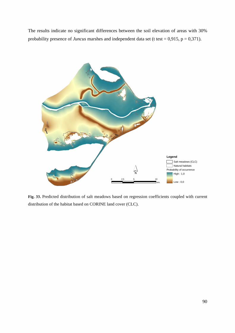
90
The results indicate no significant differences between the soil elevation of areas with 30%
probability presence of Juncus marshes and independent data set (t test = 0,915, p = 0,371).
LegendSalt meadows (CLC)Natural habitats
Probability of occurrenceHigh : 1,0
Low : 0,00 5 102,5
km.
´
Fig. 33. Predicted distribution of salt meadows based on regression coefficients coupled with current
distribution of the habitat based on CORINE land cover (CLC).
91
5. General conclusions
The application of predictive habitat modelling in the Ebro Delta has resulted a useful way to
analyze through GIS the potential distribution of wetland habitats and has provided the first
results on habitat modelling of this area. In addition, the method has served as exercise to
understand relationships between environment variables and distribution of habitat types at a
deltaic plain scale. However, the present distribution of the wetland habitats of the Ebro
Delta, being largely altered, has led to limitations in the general applicability of the predictive
model. The points below summarize the main results of this study according to the established
objectives:
1. To get elevation ranges of each habitat type within the altitude gradient of the Delta
by a digital elevation model (DEM). To validate them with field data.
The largest area of wetland habitats is concentrated between 1 and 1,5 meters due to the
presence of rice fields in this elevation range. Excluding rice fields, natural habitats have been
occupy 35% of the Delta plain between 0,0 to 0,5 m of soil elevation. In terms of elevation
zonation, we conclude that its existence is present within the topographical gradient of the
deltaic plain.
Elevation ranges of each wetland habitat seem to be concordant with literature cited, despite
the method obtaining elevation data (LIDAR) would not be appropriate in the case of coastal
lagoons. In addition, the high precision of the DEM must be taken into account when
attempting to interpret elevation metrics of some habitats (i.e reed beds or tidal flats) due to
existence of micro-topography.
The mean soil elevation of Salicornia-type marshes and reed beds (Phragmites) based on the
digital map did not adjust to independent data obtained by field transects. In contrast, salt
meadows have shown no differences between the two data sets. The difference agreement in
the first case can be attributed either errors in classification (the allocation of a category to
each tile) (Felicísimo and Gago 2002) or insufficient coverage of its elevation ranges.
92
However, the use of independent data to evaluate habitat distributions is a key step in
ecological studies.
2. To calculate distance ranges from the geographical position of each habitat type
relative to the river and marine influence, which are determined from delta hydrologic
boundaries.
Variables relating to marine and riverine influence in the deltaic plain, e.g. distance to outer
coast, distance to river mouth and distance to inner border, play a key role in explaining the
geographical position of wetland habitats. Their importance is probably linked to the fact that
these variables are related to the hydrological influences of Delta boundaries.
As we expected, the current distribution of habitat patches is related in part with their relative
position to hydrological alteration elements (i.e. distances to rice fields, channels and roads).
These habitats shown higher soil elevations near roads and channels. However with this
approach the hydrological effect may be difficult to discern since the proximity of human
infrastructures does not always mean direct effect on the habitats.
3. To apply the predictive model in a Geographic Information System (GIS) to obtain
maps of probability of presence for each habitat.
Multiple logistic regression (MLR), was considered a valid statistical approach for modelling
since the response variable is a categorical entity (i.e. presence/absence habitat type). After
reviewing scientific literature we conclude that such approach has not been widely applied in
deltas after.
Variables describing the distribution of wetland habitats in the logistic regressions models
were related with soil elevation in the case of habitats with higher elevation (dunes/beaches,
Cladium-type marshes, rice fields and riparian vegetation), whereas distance to outer coast
explained the distribution of habitats with lower elevations (coastal lagoons, tidal flats,
93
Salicornia marshes and reed beds). Distance to river channel and outer coast represents an
important variable determining the distribution of the salt meadows.
However, the use of the model for the whole Delta has shown several limitations that can be
attributed to the low representation of some wetland habitats at the present. Distribution of
several habitats (salt meadows and riparian vegetation mainly) have been drastically reduced
due to human occupation in since beginning the twentieth century. This implies a low surface
in the CORINE land cover and, therefore, the modelling exercise showed a low reliability of
the predicted distribution within the deltaic plain. Nevertheless, our mapping exercise
represents an interesting approach to visualize the predicted distribution of the habitats in
natural areas and to analyze how the human influence alters the natural habitats.
In the predictive habitat modelling one type of problem may possibly be encountered with the
total number of variables included in the model. Our initial hypotheses has been demonstrated
since wetland distribution is influenced by elevation, distances to river/sea influences and
distances to hydrologic alteration sources. But it when logistic regression is applied, the
inclusion of 11 variables partially related has likely introduced some noise in the model that
should be analyzed. Therefore, when applying this model in GIS environment, the probability
occurrence maps of habitats should be interpreted carefully. An important future effort should
consider applying the predictive model over the whole Delta with different environment
predictors (e.g. soil salinity or climatic variables).
94
6. References
Adam P. 1993. Saltmarsh ecology. Cambridge Univ Pr. Álvarez-Arbesú R. and Felicísimo A. 2002. GIS and logistic regression as tools for environmental management: a coastal cliff vegetation model in Northern Spain. Management Information Systems: 215-224. Álvarez-Rogel J., Carrasco L., Marín C.M. and Martínez-Sánchez J.J. 2007. Soils of a dune coastal salt marsh system in relation to groundwater level, micro-topography and vegetation under a semiarid Mediterranean climate in SE Spain. Catena 69: 111-121. Austin M. and Smith T. 1989. A new model for the continuum concept. Plant Ecology 83: 35-47. Badosa A., Boix D., Brucet S., López-Flores R. and Quintana X.D. 2006. Nutrients and zooplankton composition and dynamics in relation to the hydrological pattern in a confined Mediterranean salt marsh (NE Iberian Peninsula). Estuarine, Coastal and Shelf Science 66: 513-522. Bockelmann A.-C., Bakker J.P., Neuhaus R. and Lage J. 2002. The relation between vegetation zonation, elevation and inundation frequency in a Wadden Sea salt marsh. Aquatic Botany 73: 211-221. Bouma T.J., De Vries M.B., Low E., Kusters L., Herman P.M.J., Tanczos I.C., Temmerman S., Hesselink A., Meire P. and van Regenmortel S. 2005. Flow hydrodynamics on a mudflat and in salt marsh vegetation: identifying general relationships for habitat characterisations. Hydrobiologia 540: 259-274. Brown D.G. 1994. Predicting vegetation types at treeline using topography and biophysical disturbance variables. Journal of Vegetation Science 5: 641-656. Burrough P.A., McDonnell R.A. and McDonnell R. 1998. Principles of geographical information systems. Oxford university press Oxford. Camp J. and Delgado M. 1987. Hidrografía de las bahías del delta del Ebro. Investigaciones Pesqueras 51: 351-369. Capítulo A.R., España A., Ibàñez C. and Prat N. 1994. Limnology of natural wells in the Ebro Delta (NE Spain). In Sladeckova A. (ed.), International Association of Theoretical and Applied Limnology, Proceedings, Vol 25, Pt 3, pp. 1430-1433. Carreras J. and Diego F. 2007. Cartografia dels hàbitats a Catalunya 1: 50.000. Generalitat de Catalunya. Data retrieval at: http://mediambient. gencat. net/cat/el_medi/habitats/inici. htm (June 2007). Comín F.A. and Ferrer X. 1999. Distribució i ecologia dels macròfits submergits del delta de l'Ebre. Butlletí de la Institució Catalana d'Història Natural: 111-117. Comín F.A., Menéndez M. and Martín M. 1991. Short-term effects of decreasing water discharge on the chemical and biological characteristics of eutrophic coastal lagoons. Memorie dell'Istituto italiano di idrobiologia dott. Marco de Marchi 48: 9. Communities E. 1991. CORINE biotopes - The design, compilation and use of an inventory of sites of major importance for nature conservation in the European Community, Luxembourg. p. 132.
95
Communities E. 2003. Interpretation Manual of European Union Habitats-EUR 25. European Commission, DG-XI-D-2, Brussels. Coops H., van den Brink F.W.B. and van der Velde G. 1996. Growth and morphological responses of four helophyte species in an experimental water-depth gradient. Aquatic Botany 54: 11-24. Corsi F., Duprè E. and Boitani L. 1999. A large scale model of wolf distribution in Italy for conservation planning. Conservation Biology 13: 150-159. Curcó A. 2001. La vegetación del delta del Ebro (V): las comunidades helofíticas e higrófilas (clases Phragmiti-Magnocaricetea y Molinio-Arrhebatheretea). Lazaroa: 67-81. Curcó A. 2006. Aiguamolls litorals del Delta de l'Ebre: síntesi del medi físic d'una zona humida del litoral. L'Atzavara 14: 55-72. Curcó A., Canicio C. and Ibàñez C. 1995. Mapa d'hàbitats potencials del Delta de l'Ebre. Butll. Parc Natural Delta Ebre 9: 4-12. Curcó A., Ibàñez C., Day J.W. and Prat N. 2002. Net primary production and decomposition of salt marshes of the Ebre Delta (Catalonia, Spain). Estuaries and Coasts 25: 309-324. Custer J.F., Eveleigh T., Klemas V. and Wells I. 1986. Application of LANDSAT data and synoptic remote sensing to predictive models for prehistoric archaeological sites: an example from the Delaware coastal plain. American Antiquity: 572-588. Davis F.W. and Goetz S. 1990. Modeling vegetation pattern using digital terrain data. Landscape ecology 4: 69-80. Day J., Britsch L., Hawes S., Shaffer G., Reed D. and Cahoon D. 2000. Pattern and process of land loss in the Mississippi Delta: A Spatial and temporal analysis of wetland habitat change. Estuaries and Coasts 23: 425-438. Espinar J.L. 2009. 1410 Pastizales salinos mediterráneos (Juncetalia maritimi). In VV.AA. (ed.), Bases ecológicas preliminares para la conservación de los tipos de hábitat de interés comunitario en España p. 77, Madrid. Felicísimo A. and Gago L.M.S. 2002. Thematic and spatial accuracy: a comparison of the Corine Land Cover with the Forestry Map of Spain. pp. 109-118. Palma, Balearic Islands Spain. Felicísimo A.M. 2003. Uses of spatial predictive models in forested areas territorial planning. In CIOT-IV International Conference on Spatial Planning, pp. 2-4. Felicísimo A.M., Frances E., Fernández J.M., González-Diez A. and Varas J. 2002. Modeling the potential distribution of forests with a GIS. Photogrammetric Engineering and Remote Sensing 68: 455-461. Filipe A.F., Cowx I.G. and Collares-Pereira M.J. 2002. Spatial modelling of freshwater fish in semi-arid river systems: a tool for conservation. River Research and Applications 18: 123-136. Franklin J. 1995. Predictive vegetation mapping: geographic modelling of biospatial patterns in relation to environmental gradients. Progress in Physical Geography 19: 474. Franklin J., McCullough P. and Gray C. 2000. Terrain variables used for predictive mapping of vegetation communities in southern California. In Wilson J. P. and Gallant J. C. (eds.), Terrain analysis: principles and applications.
96
Giasson E., Clarke R.T., Inda Junior A.V., Merten G.H. and Tornquist C.G. 2006. Digital soil mapping using multiple logistic regression on terrain parameters in southern Brazil. Scientia Agricola 63: 262-268. Guisan A., Theurillat J.P. and Kienast F. 1998. Predicting the potential distribution of plant species in an alpine environment. Journal of Vegetation Science 9: 65-74. Guisan A., Weiss S.B. and Weiss A.D. 1999. GLM versus CCA spatial modeling of plant species distribution. Plant Ecology 143: 107-122. Guisan A. and Zimmermann N.E. 2000. Predictive habitat distribution models in ecology. Ecological modelling 135: 147-186. Hickey D. and Bruce E. 2010. Examining Tidal Inundation and Salt Marsh Vegetation Distribution Patterns using Spatial Analysis (Botany Bay, Australia). Journal of Coastal Research 26: 94-102. Hosmer D.W. and Lemeshow S. 2000. Applied logistic regression. Wiley-Interscience. Ibànez C., Canicio A., Day J.W. and Curcó A. 1997. Morphologic development, relative sea level rise and sustainable management of water and sediment in the Ebre Delta, Spain. Journal of Coastal Conservation 3: 191-202. Ibàñez C., Canicio C., Curcó A., Day J.W. and Prat N. 1996. Evaluation of vertical accretion and subsidence rates. Departament d'Ecologia, Universitat de Barcelona, Barcelona. pp. 43-65. Ibàñez C., Curco A., Day J.W. and Prat N. 2002. Structure and productivity of microtidal Mediterranean coastal marshes. In Weinstein M. P. and Kreeger D. A. (eds.), Concepts and controversies in tidal marsh ecology, pp. 107-136. Ibàñez C., Pont D. and Prat N. 1997. Characterization of the Ebre and Rhone estuaries: A basis for defining and classifying salt-wedge estuaries. Limnology and Oceanography: 89-101. Ibàñez C., Sharpe P.J., Day J.W., Day J.N. and Prat N. 2010. Vertical Accretion and Relative Sea Level Rise in the Ebro Delta Wetlands (Catalonia, Spain). Wetlands: 1-10. IPCC C.C. 2001. Intergovernmental Panel on Climate Change. Third Assessment Report. Jiménez J.A. 1996. Evolución costera en el Delta del Ebro. Un proceso a diferentes escalas de tiempo y espacio, Universidad Politecnica de Catalunya: Barcelona. 271pp. Jiménez J.A. and Sánchez-Arcilla A. 1993. Medium-term coastal response at the Ebro delta, Spain. Marine Geology 114: 105-118. Kjerfve B. 1994. Coastal lagoon processes. Elsevier Science Ltd. Korakis G. and Gerasimidis A. 2006. Coastal and halophytic habitats and their flora in Evrotas Delta (SE Peloponnisos, Greece). Journal of Biological Research 6: 155-166. Lenssen J.P.M., Menting F.B.J., Van der Putten W.H. and Blom C. 2000. Variation in species composition and species richness within Phragmites australis dominated riparian zones. Plant Ecology 147: 137-146. Llebot C., Spitz Y.H., Solé J. and Estrada M. 2010. The role of inorganic nutrients and dissolved organic phosphorus in the phytoplankton dynamics of a Mediterranean bay: A modeling study. Journal of Marine Systems 83: 192-209.
97
Maldonado A. 1972. El delta del Ebro: estudio sedimentológico y estratigráfico, Universitat de Barcelona: Barcelona. 1-486pp. Mañosa S., Mateo R. and Guitart R. 2001. A review of the effects of agricultural and industrial contamination on the Ebro delta biota and wildlife. Environmental Monitoring and Assessment 71: 187-205. Martínez-Alonso M., Mir J., Caumette P., Gaju N., Guerrero R. and Esteve I. 2004. Distribution of phototrophic populations and primary production in a microbial mat from the Ebro Delta, Spain. International Microbiology 7: 19-26. Menéndez M. and Comin F. 2000. Spring and summer proliferation of floating macroalgae in a Mediterranean coastal lagoon (Tancada Lagoon, Ebro Delta, NE Spain). Estuarine, Coastal and Shelf Science 51: 215-226. Menéndez M., Hernández O. and Comín F.A. 2002. Spatial distribution and ecophysiological characteristics of macrophytes in a Mediterranean coastal lagoon. Estuarine Coastal and Shelf Science 55: 403-413. Mikhailova M.V. 2003. Transformation of the Ebro River Delta under the Impact of Intense Human-Induced Reduction of Sediment Runoff. Water Resources 30: 370-378. Mir J., Martínez-Alonso M. and Esteve I. 2000. Estudi de la biocenosi deIs tapissos microbians del delta de l'Ebre. Butlletí de la Institució Catalana d'Història Natural 68: 112-133. Moffett K.B., Robinson D.A. and Gorelick S.M. 2010. Relationship of Salt Marsh Vegetation Zonation to Spatial Patterns in Soil Moisture, Salinity, and Topography. Ecosystems 13: 1287-1302. Moran J., Kelly S., Sheehy S.M. and Gormally M. 2008. The use of GIS techniques to quantify the hydrological regime of a karst wetland (Skealoghan turlough) in Ireland. Applied Vegetation Science 11: 25-U31. Narumalani S., Jensen J.R., Althausen J.D., Burkhalter S. and Mackey H.E. 1997. Aquatic macrophyte modeling using GIS and logistic multiple regression. Photogrammetric Engineering and Remote Sensing 63: 41-49. Pearce J. and Ferrier S. 2000. Evaluating the predictive performance of habitat models developed using logistic regression. Ecological modelling 133: 225-245. Pérez-Ruzafa A., Fernández A.I., Marcos C., Gilabert J., Quispe J.I. and García-Charton J.A. 2005. Spatial and temporal variations of hydrological conditions, nutrients and chlorophyll a in a Mediterranean coastal lagoon (Mar Menor, Spain). Hydrobiologia 550: 11-27. Pont D., Day J.W., Hensel P., Franquet E., Torre F., Rioual P., Ibàñez C. and Coulet E. 2002. Response scenarios for the deltaic plain of the Rhône in the face of an acceleration in the rate of sea-level rise with special attention to Salicornia-type environments. Estuaries and Coasts 25: 337-358. Ríos J.J.M., Pérez E.C., Castro C.M.V. and Vera J.J.Q. 2005. Modeling and spatial distribution of Oregano (Lippia graveolens H.B.K.) at Mapimí Biosphere Reserve in Durango, Mexico In Suelos ecuatoriales. Romao C. 1996. Interpretation manual of European union habitats: version EUR 15.
98
Rovira A. and Ibàñez C. 2007. Sediment management options for the lower Ebro River and its delta. Journal of Soils and Sediments 7: 285-295. Rüger N., Schlüter M. and Matthies M. 2005. A fuzzy habitat suitability index for Populus euphratica in the Northern Amudarya delta (Uzbekistan). Ecological modelling 184: 313-328. Sakamaki T., Nishimura O. and Sudo R. 2006. Tidal time-scale variation in nutrient flux across the sediment-water interface of an estuarine tidal flat. Estuarine, Coastal and Shelf Science 67: 653-663. Shoutis L., Patten D.T. and McGlynn B. 2010. Terrain-based predictive modeling of riparian vegetation in a Northern Rocky Mountain watershed. Wetlands 30: 621-633. Silvestri S., Defina A. and Marani M. 2005. Tidal regime, salinity and salt marsh plant zonation. Estuarine, Coastal and Shelf Science 62: 119-130. Silvestri S. and Marani M. 2004. Salt-marsh vegetation and morphology: Basic physiology, modelling and remote sensing observations. Coastal and Estuarine Studies 59: 5-25. Spellerberg I.F. 1994. Evaluation and assessment for conservation: ecological guidelines for determining priorities for nature conservation. Springer. Squires L. and Valk A.G.V.d. 1992. Water-depth tolerances of the dominant emergent macrophytes of the Delta Marsh, Manitoba. Canadian Journal of Botany 70: 1860-1867. Syphard A.D. and Franklin J. 2010. Species traits affect the performance of species distribution models for plants in southern California. Journal of Vegetation Science 21: 177-189. Tarkesh M. and Jetschke G. 2012. Comparison of six correlative models in predictive vegetation mapping on a local scale. Environmental and Ecological Statistics: 1-21. Turner M.G., Gergel S.E., Dixon M.D. and Miller J.R. 2004. Distribution and abundance of trees in floodplain forests of the Wisconsin River: environmental influences at different scales. Journal of Vegetation Science 15: 729-738. Valdemoro H.I., Sanchez-Arcilla A. and Jimenez J.A. 2007. Coastal dynamics and wetlands stability. The Ebro delta case. Hydrobiologia 577: 17-29. van Horssen P.W., Schot P.P. and Barendregt A. 1999. A GIS-based plant prediction model for wetland ecosystems. Landscape ecology 14: 253-265. vandeRijt C., Hazelhoff L. and Blom C. 1996. Vegetation zonation in a former tidal area: A vegetation-type response model based on DCA and logistic regression using GIS. Journal of Vegetation Science 7: 505-518. Vigo J., Carreras J. and Ferré A. 2006. Manual dels hàbitats de Catalunya. Vol. I-VIII. Departament de Medi Ambient i Habitatge, Generalitat de Catalunya, Barcelona. Vogiatzakis I.N. 2003. GIS-based Modelling and Ecology: A Review of Tools and Methods. Vogiatzakis I.N. and Griffiths G.H. 2006. A GIS-based empirical model for vegetation prediction in Lefka Ori, Crete. Plant Ecology 184: 311-323. Vogiatzakis I.N., Mannion A.M. and Griffiths G.H. 2006. Mediterranean ecosystems: problems and tools for conservation. Progress in Physical Geography 30: 175-200.
99
Welch B., Davis C. and Gates R. 2006. Dominant environmental factors in wetland plant communities invaded by Phragmites australis in East Harbor, Ohio, USA. Wetlands Ecology and Management 14: 511-525. Whittaker R.H. 1967. GRADIENT ANALYSIS OF VEGETATION*. Biological Reviews 42: 207-264. Xie Z.X., Liu Z.W., Jones J.W., Higer A.L. and Telis P.A. 2011. Landscape unit based digital elevation model development for the freshwater wetlands within the Arthur C. Marshall Loxahatchee National Wildlife Refuge, Southeastern Florida. Applied Geography 31: 401-412. Zar J.H. 1999. Biostatistical analysis. Prentice Hall New Jersey 4. Zare Chahouki M., Azarnivand H., Jafari M. and Tavili A. 2010. Multivariate statistical methods as a tool for model-based prediction of vegetation types. Russian Journal of Ecology 41: 84-94.