DEPARTAMENTO DE BROMATOLOGÍA Y TECNOLOGÍA DE LOS ...
194
UNIVERSIDAD DE CÓRDOBA E.T.S. DE INGENIERÍA AGRONÓMICA Y DE MONTES DEPARTAMENTO DE BROMATOLOGÍA Y TECNOLOGÍA DE LOS ALIMENTOS “Determinación no destructiva de parámetros de calidad en uvas, racimos y mostos mediante Espectroscopía de Reflectancia en el Infrarrojo Cercano” TESIS DOCTORAL Virginia González Caballero Directoras: Dra. Mª Teresa Sánchez Pineda de las Infantas Dra. Dolores Pérez Marín 2012
Transcript of DEPARTAMENTO DE BROMATOLOGÍA Y TECNOLOGÍA DE LOS ...

UNIVERSIDAD DE CÓRDOBA
E.T.S. DE INGENIERÍA AGRONÓMICA Y DE MONTES DEPARTAMENTO DE BROMATOLOGÍA Y TECNOLOGÍA DE LOS ALIMENTOS
“Determinación no destructiva de parámetros de calidad en uvas, racimos y mostos mediante Espectroscopía de
Reflectancia en el Infrarrojo Cercano”
TESIS DOCTORAL
Virginia González Caballero
Directoras:
Dra. Mª Teresa Sánchez Pineda de las Infantas Dra. Dolores Pérez Marín
2012

TÍTULO: Determinación no destructiva de parámetros de calidad en uvas, racimos
y mostos mediante Espectroscopía de Reflectancia en el Infrarrojo Cercano
AUTOR: Virginia González Caballero
© Edita: Servicio de Publicaciones de la Universidad de Córdoba. 2012Campus de RabanalesCtra. Nacional IV, Km. 396 A14071 Córdoba
www.uco.es/[email protected]

“Determinación no destructiva de parámetros de calidad en uvas, racimos y mostos mediante Espectroscopía de
Reflectancia en el Infrarrojo Cercano”
TESIS
para aspirar al grado de Doctor por la Universidad de Córdoba presentada por la
Licenciada en Enología Dña. Virginia González Caballero
La Doctoranda
Fdo.: Virginia González Caballero
VºBº Las Directoras
Fdo.: Profª. Dra. Mª Teresa Sánchez Fdo.: Profª. Dra. Dolores Pérez Marín Pineda de las Infantas
2012
Departamento de Bromatología
y Tecnología de los Alimentos


Mª TERESA SÁNCHEZ PINEDA DE LAS INFANTAS, Catedrática de Universidad del
Departamento de Bromatología y Tecnología de los Alimentos de la Universidad de
Córdoba y DOLORES PÉREZ MARÍN, Profesora Titular de Universidad del
Departamento de Producción Animal de la Universidad de Córdoba
I N F O R M A N:
Que la Tesis titulada “DETERMINACIÓN NO DESTRUCTIVA DE
PARÁMETROS DE CALIDAD EN UVAS, RACIMOS Y MOSTOS MEDIANTE
ESPECTROSCOPÍA DE REFLECTANCIA EN EL INFRARROJO CERCANO”,
de la que es autora Dña. Virginia González Caballero, ha sido realizada bajo nuestra
dirección durante los años 2008, 2009, 2010, 2011 y 2012; y cumple las condiciones
académicas exigidas por la Legislación vigente para optar al título de Doctor por la
Universidad de Córdoba.
Y para que conste a los efectos oportunos firman el presente informe en Córdoba
a 12 de abril de 2012
Fdo.: Profª. Dra. Mª Teresa Sánchez Fdo.: Profª. Dra. Dolores Pérez Marín Pineda de las Infantas
Departamento de Bromatología
y Tecnología de los Alimentos

TÍTULO DE LA TESIS: DETERMINACIÓN NO DESTRUCTIVA DE PARÁMETROS DE CALIDAD EN UVAS, RACIMOS Y MOSTOS MEDIANTE ESPECTROSCOPÍA DE REFLECTANCIA EN EL INFRARROJO CERCANO DOCTORANDA: VIRGINIA GONZÁLEZ CABALLERO
INFORME RAZONADO DE LAS DIRECTORAS DE LA TESIS (se hará mención a la evolución y desarrollo de la tesis, así como a trabajos y publicaciones derivados de la misma).
La Tesis cuyo título se menciona arriba ha podido adaptarse, desde sus inicios, a
la metodología y el diseño programados, derivando todo ello en la obtención de
resultados de indudable relevancia científica y tecnológica.
En primer lugar, hay que destacar que del trabajo de esta Tesis se han
establecido las bases científico-técnicas para el desarrollo de modelos de predicción
NIRS cuantitativos y se han obtenido un amplio abanico de aplicaciones NIRS relativas
a la determinación de parámetros de calidad interna de uva, relacionados principalmente
con el contenido de azúcares y la acidez, para la cuantificación no destructiva de los
cambios químicos que tienen lugar durante la maduración de los racimos en la vid, y
para facilitar la toma de decisiones sobre el momento óptimo de cosecha. Se han
ensayado distintas formas de presentación de muestra a los instrumentos: racimo, grano
y mosto, obteniéndose con el racimo, modelos de adecuada capacidad predictiva,
similar a la obtenida con el grano, lo que permite el realizar análisis in situ, en campo, y
en la recepción en la industria, facilitando de esta forma una recolección selectiva de los
racimos de uva, dependiendo del tipo de vino a elaborar. Por otro lado, se han
desarrollado modelos NIRS destinados a la determinación de los cambios físicos-
químicos (disminución de la masa volúmica) que se producen durante la fermentación
alcohólica, llevando a cabo la aplicación de esta tecnología en el proceso completo de

transformación de la uva en vino. Asimismo, se han determinado para las distintas
aplicaciones desarrolladas en este Trabajo de Investigación los instrumentos NIRS más
idóneos en función, tanto de las necesidades del campo y de la industria de enológica,
como de los parámetros de interés elegidos y de las características intrínsecas del
producto. Lo anteriormente expuesto justifica plenamente que la forma más idónea de
presentación de esta Tesis Doctoral sea el compendio de publicaciones científicas.
La doctoranda ha tenido la posibilidad de formarse, no sólo en aspectos
científicos-técnicos ligados a la tecnología NIRS, sino también relacionados con la
ingeniería y tecnología enológica. Asimismo, la doctoranda ha complementado su
formación realizando una estancia de 3 meses en el Department of Science of
Production and Innovation in the Mediterranean Agriculture & Food Systems (PRIME)
de la Università degli Studi di Foggia (Italia) bajo la supervisión del Prof. Dr. Giancarlo
Colelli.
Los trabajos publicados relacionados con los resultados de la Tesis son los
siguientes:
1. González-Caballero, V.; Sánchez, M.T.; López, M.I.; Pérez-Marín, D.
2010. First steps towards the development of a non-destructive technique
for the quality control of wine grapes during on-vine ripening and on
arrival at the winery. Journal of Food Engineering 101, 158-165.
2. González-Caballero, V.; Pérez-Marín, D.; López, M.I.; Sánchez, M.T.
2011. Optimization of NIR spectral data management for quality control
of grape bunches during on-vine ripening. Sensors, 11, 6109-6124.
3. González-Caballero, V.; Sánchez, M.T.; López, M.I.; Pérez-Marín, D.
2012. On-Vine Monitoring of Grape Ripening Using Near-Infrared
Spectroscopy. Food Analytical Methods. DOI 10.1007/s12161-012-
9389-3. Online First, 13 March 2012.

4. Fernández-Novales, J.; López, M.I.; González-Caballero, V.; Ramírez, P.;
Sánchez, M.T. 2011. Feasibility of using a miniature NIR spectrometer to
measure volumic mass during alcoholic fermentation. International Journal
of Food Sciences and Nutrition 62, 353-359.
Por todo ello, se autoriza la presentación de la tesis doctoral.
Córdoba, 10 de abril de 2012
Fdo.: María Teresa Sánchez Fdo.: Dolores Pérez Marín Pineda de las Infantas

A mi madre,
ejemplo de mujer trabajadora
por su tesón, sacrificio
y profesionalidad.


Agradecimientos


Deseo expresar mi sincera gratitud y reconocimiento a todas las personas que han
hecho posible la realización de este Trabajo de Investigación:
A la Dra. María Teresa Sánchez Pineda de las Infantas, Catedrática de Universidad
del Departamento de Bromatología y Tecnología de los Alimentos de la Universidad de
Córdoba, y codirectora de esta Tesis.
A la Dra. Dolores Pérez Marín, Profesora Titular de Universidad del Departamento
de Producción Animal de la Universidad de Córdoba, y codirectora de esta Tesis.
A la Dra. Mª Isabel López Infante, Profesora Asociada del Departamento de
Bromatología y Tecnología de los Alimentos de la Universidad de Córdoba.
A la Dra. Brígida Jiménez Herrera, Directora del IFAPA Centro de Cabra, de la
Consejería de Agricultura y Pesca de la Junta de Andalucía, así como a todos mis
compañeros en este Centro. Agradezco especialmente la colaboración de la Dra. Pilar
Ramírez, de D. José Marín, de D. Francisco Zamorano, de Dña. Anabel Lucena y de D.
José Morales.
A los Departamentos de Bromatología y Tecnología de los Alimentos y
Producción Animal de la Universidad de Córdoba.
A mi familia, por su apoyo incondicional durante todo el tiempo que ha durado la
realización de esta Tesis Doctoral.
A mi marido Juan, por su inmensa ayuda, sin él no hubiera finalizado esta Tesis
Doctoral.
Por último, a todos aquellos que durante estos años se han interesado por el
desarrollo de esta Tesis, muchas gracias.


Índice


Índice
RESUMEN 3
ABSTRACT 7
Capítulo 1. INTRODUCCIÓN 11
Capítulo 2. OBJETIVOS 17
2.1. OBJETIVO GENERAL 17
2.2. OBJETIVOS ESPECÍFICOS 17
Capítulo 3. REVISIÓN BIBLIOGRÁFICA 21
3.1. INTRODUCCIÓN 21
3.2. EL SECTOR VITIVINÍCOLA: PRODUCCIÓN Y
COMERCIALIZACIÓN. 22
3.3. LA CALIDAD DE LA UVA DESDE EL VIÑEDO 24
3.3.1. El material vegetal 27
3.3.2. Factores precosecha 28
3.3.2.1. El suelo 28
3.3.2.2. El clima 30
3.3.3. Factores humanos: Técnicas de cultivo 31
3.3.3.1. La poda 31
3.3.3.2. El riego y el abonado 33
3.4. LA MADURACIÓN 34
3.4.1. Seguimiento de maduración 35
3.4.2. La toma de muestras 36
3.4.3. Determinación de la fecha de vendimia 37
3.5. MÉTODOS DE ANÁLISIS TRADICIONALES DE DETERMINACIÓN
DE LOS PRINCIPALES PARÁMETROS DE CALIDAD EN UVAS 39
3.5.1. Contenido en sólidos solubles totales 39
3.5.2. Azúcares reductores 40
3.5.3. Acidez titulable y pH 41
3.5.4. Ácido tartárico 41
3.5.5. Ácido málico 42
3.5.6. Potasio 43
3.6. LA TECNOLOGÍA DE ESPECTROSCOPÍA DE REFLECTANCIA EN
EL INFRARROJO CERCANO (NIRS) 43

Índice ______________________________________________________________________
3.6.1. Bases teóricas 45
3.6.2 Bases instrumentales 47
3.6.3. Análisis quimiométrico de datos espectroscópicos NIRS. 54
3.6.3.1. Análisis de Componentes Principales (ACP) 56
3.6.3.2 Análisis cuantitativo. Calibración multivariante 57
3.6.3.3. Análisis cualitativo 63
3.7. APLICACIÓN DE LA TECNOLOGÍA NIRS PARA EL CONTROL DE
CALIDAD Y TRAZABILIDAD EN EL SECTOR VITIVINÍCOLA 68
3.7.1. Determinaciones cuantitativas de los principales parámetros de calidad
en uva utilizando NIRS 69
3.7.1.1. Determinaciones cuantitativas at-line de los principales parámetros de
calidad en uva utilizando NIRS 71
3.7.1.2. Determinaciones cuantitativas in situ de los principales parámetros de
calidad en uva utilizando NIRS 79
3.8. REFLEXIONES FINALES SOBRE EL ESTADO DE DESARROLLO DEL
ANÁLISIS NIRS EN LA INDUSTRIA VITIVINÍCOLA 84
Capítulo 4. LA TECNOLOGÍA NIRS PARA LA PREDICCIÓN DE
PARÁMETROS DE CALIDAD INTERNA, DETERMINACIÓN DEL
MOMENTO ÓPTIMO DE COSECHA Y CONTROL DE CALIDAD
Y TRAZABILIDAD EN LA INDUSTRIA VITIVINÍCOLA 89
4.1. FIRST STEPS TOWARDS THE DEVELOPMENT OF A NON-
DESTRUCTIVE TECHNIQUE FOR THE QUALITY CONTROL OF WINE
GRAPES DURING ON-VINE RIPENING AND ON ARRIVAL AT THE
WINERY. JOURNAL OF FOOD ENGINEERING 101, 158–165 (2010) 89
4.2. EVALUATION OF DIFFERENT REGRESSION STRATEGIES FOR
INTERNAL QUALITY CONTROL OF GRAPE BUNCHES DURING ON-
VINE RIPENING. SENSORS 11, 6109-6124 (2011) 99
4.3. ON-VINE MONITORING OF GRAPE RIPENING USING NEAR
INFRARED SPECTROSCOPY. FOOD ANALYTICAL METHODS (2012) 117
4.4. FEASIBILITY OF USING A MINIATURE NIR SPECTROMETER TO
MEASURE VOLUMIC MASS DURING ALCOHOLIC FERMENTATION.
INTERNATIONAL JOURNAL OF FOOD SCIENCES AND NUTRITION 62,
353–359 (2011) 129

Índice
Chapter 5. CONCLUSIONS 141
Capítulo 6. BIBLIOGRAFÍA 147

Índice
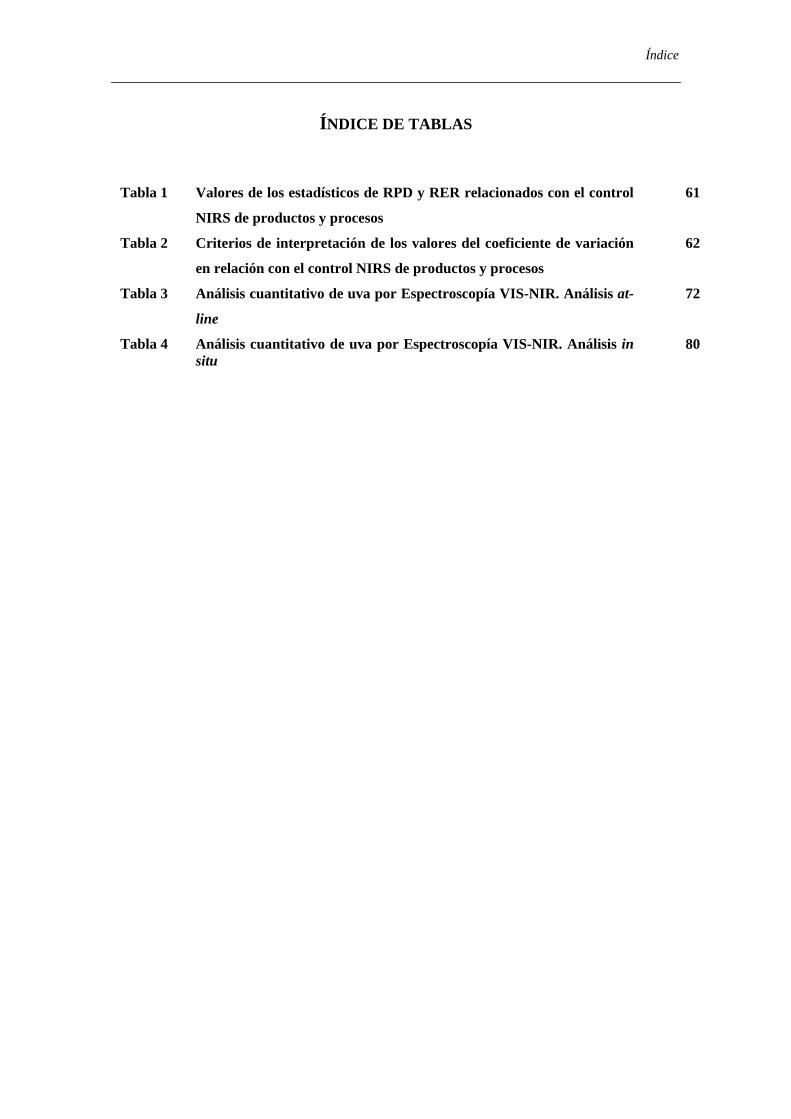
ÍNDICE DE TABLAS
Tabla 1 Valores de los estadísticos de RPD y RER relacionados con el control
NIRS de productos y procesos
61
Tabla 2 Criterios de interpretación de los valores del coeficiente de variación
en relación con el control NIRS de productos y procesos
62
Tabla 3 Análisis cuantitativo de uva por Espectroscopía VIS-NIR. Análisis at-
line
72
Tabla 4 Análisis cuantitativo de uva por Espectroscopía VIS-NIR. Análisis in situ
80


Índice
ÍNDICE DE FIGURAS
Figura 1 Formas de análisis NIRS de los productos agroalimentarios
(adaptado de Kawano, 2002)
48
Figura 2 Componentes básicos de un instrumento NIRS 50
Figura 3 Componentes básicos de un instrumento NIRS de red de diodos 51
Figura 4 Componentes básicos de un instrumento NIRS-MEMS 52
Figura 5 Instrumento portátil NIR-MEMS PhazirTM 53


Abreviaturas

Abreviaturas ______________________________________________________________________
A: Absorbancia.
ACP: Análisis de Componentes Principales.
AT: Acidez titulable.
CE: Comunidad Europea.
CH: Enlace carbono-hidrógeno.
CP: Componente Principal.
CPs: Componentes Principales.
CV: Coeficiente de Variación de un constituyente químico, calculado como dt/media.
CVETL: Coeficiente de Variación del estadístico ETL, calculado como ETL/media.
CVETVC: Coeficiente de Variación del estadístico ETVC, calculado como
ETVC/media.
dt: Desviación típica.
DT: Detrending.
DTS: Digital Transform Spectroscopy.
ETC: Error Típico de Calibración.
ETL: Error Típico de Laboratorio (método de referencia).
ETP: Error Típico de Predicción.
ETSIAM: Escuela Técnica Superior de Ingeniería Agronómica y de Montes.
ETVC: Error Típico de Validación Cruzada.
EE.UU.: Estados Unidos.
FAO: Organización de Naciones Unidas para la Agricultura y la Alimentación.
FT-NIR: NIR con transformada de Fourier.
H: Distancia de H, estadístico análogo a la Distancia de Mahalanobis.
HR: Humedad relativa.
MAPA: Ministerio de Agricultura, Pesca y Alimentación.
MARM: Ministerio de Medio Ambiente y Medio Rural y Marino.
MEMS: Micro-Electro-Mechanical System.
MIR: Mid Infrared, Infrarrojo medio.
MPLS: Modified Partial Least Squares, Mínimos Cuadrados Parciales Modificados.
MSC: Multiplicative Scatter Correction, Corrección multiplicativa del efecto “scatter”.
NH: Enlace nitrógeno-hidrógeno.
NIR: Near Infrared, Infrarrojo cercano.
NIRS: Near Infrared Spectrocopy, Espectroscopía en el infrarrojo cercano.
nm: Nanómetros.

Abreviaturas ______________________________________________________________________
OH: Enlace oxigeno-hidrógeno.
PLS: Partial Least Squares, Mínimos Cuadrados Parciales.
r y R: Coeficientes de correlación.
r2 y R2: Coeficientes de determinación.
RCP: Regresión en Componentes Principales.
RER: Range Error Ratio, Cociente entre el intervalo de composición de los datos de
referencia y el ETVC.
RLM: Regresión Lineal Múltiple.
RPD: Residual Predictive Deviation, Cociente entre la desviación típica de la
composición de los datos de referencia y el ETVC.
SNV: Standard Normal Variate.
SST: Sólidos solubles totales.
T: Estadístico T, análogo a una t de Student.
UCO: Universidad de Córdoba.
UE: Unión Europea.
UV: Ultravioleta.
VIS: Visible.

Resumen

Resumen ______________________________________________________________________
3
RESUMEN
La Espectroscopía de Infrarrojo Cercano (NIRS) se ha convertido en una técnica
analítica muy útil para la determinación no destructiva de parámetros de calidad en
alimentos, adaptándose plenamente a las exigencias de la industria vitivinícola en
términos de control de calidad y trazabilidad.
Aunque el número de aplicaciones NIRS en el proceso de elaboración de vinos
se ha incrementado en los últimos años, el uso de la espectroscopía NIR en la industria
vitivinícola se encuentra todavía en una etapa de desarrollo muy incipiente, siendo
necesaria la optimización del empleo de sensores NIRS en dicha industria. En este
sentido, la determinación de calidad de las uvas en campo y en bodega, directamente
sobre el racimo, significaría un importante avance para el sector enológico. Ello
permitiría no sólo el realizar el seguimiento del proceso de maduración en campo - lo
que facilitaría la toma de decisiones respecto al momento óptimo de vendimia - sino
también posibilitaría la rápida medición de los parámetros de calidad de la uva a su
llegada a bodega, lo que permitiría acelerar la toma de decisiones en esta etapa,
posibilitando el procesado por separado de lotes en función de la calidad inicial de la
materia prima, evaluada de forma precisa y exacta, antes de su elaboración.
El objetivo principal de esta Tesis Doctoral ha sido desarrollar modelos NIRS
precisos y robustos destinados a la determinación de los principales parámetros de
calidad interna (contenido de sólidos solubles y en azúcares reductores, pH, acidez
titulable, contenidos en ácido tartárico, ácido málico, y en potasio) de uvas de
vinificación durante su maduración en campo, en el momento de cosecha y en su
recepción en bodega, utilizando el racimo como forma de presentación de muestra a los
instrumentos, con el fin de permitir a los agricultores y bodegueros, el uso rutinario de
la tecnología NIRS en la industria vitinivinícola para predecir con mayor precisión el
momento óptimo de vendimia y la calidad inicial de las uvas a su llegada a la industria,
garantizando así la más alta calidad posible tanto de la uva como del vino a elaborar.
Con este propósito se han evaluado igualmente dos espectrofotómetros comercialmente
disponibles, uno muy adecuado para efectuar mediciones in situ, directamente en las
Resumen ______________________________________________________________________
4
cepas (espectrofotómetro basado en la tecnología MEMS) y el otro idóneo para su
utilización en las líneas de elaboración en bodega (espectrofotómetro de red de diodos).
Asimismo, el presente Trabajo de Investigación analizó la viabilidad de utilizar
un espectrofotómetro NIR miniatura, de bajo coste, para la predicción de la masa
volúmica en vinos blancos y tintos durante la fermentación alcohólica, tratando de
identificar al mismo tiempo las longitudes de onda más significativas asociadas a la
determinación de dicho parámetro.
Los resultados obtenidos permiten afirmar que la capacidad predictiva de los
modelos desarrollados para la determinación de parámetros de calidad interna en uvas,
empleando el racimo como modo de presentación de muestra, fueron similares a los
obtenidos al utilizar bayas y mosto, lo que permite la aplicación de la tecnología NIRS
para el análisis no destructivo de uvas en campo, durante la maduración de la vid, como
a su llegada a la bodega, empleando para el caso de las determinaciones in situ en cepas,
el instrumento NIR-MEMS seleccionado, mientras que en la bodega se utilizó el de red
de diodos.
En este sentido, el análisis de las uvas utilizando el racimo debe ser considerado
como un primer paso en el empleo de la tecnología NIRS para el control de calidad in
situ y en línea en la industria enológica, ya que ésta es la forma en la que se lleva a cabo
el desarrollo de las uvas en las cepas, así como su recepción en bodega. Este Trabajo de
Investigación ha sido el primer intento de utilización de la espectroscopía NIR tanto a
nivel de campo como de bodega, empleando como forma de presentación de muestra al
instrumento aquella en la que se lleva a cabo el desarrollo y recepción del fruto en la
industria vitivinícola.
Por otra parte, los resultados obtenidos confirman que la espectroscopía NIR es
sensible a los cambios físicos/químicos (disminución de la masa volúmica) que se
producen durante la fermentación alcohólica, en el rango espectral de 800 a 1050 nm.
Asimismo, se llevó cabo la identificación de seis longitudes de onda fuertemente
correlacionadas con la masa volúmica, las cuales podrían ser utilizadas para desarrollar
un instrumento simple, eficiente, de bajo costo que podría emplearse también, para
determinar el contenido de azúcares reductores en vinos durante la fermentación.

Resumen ______________________________________________________________________
5
Por tanto, los resultados obtenidos de este Trabajo de Investigación muestran la
viabilidad de la utilización de la tecnología NIRS para cuantificar los cambios químicos
que ocurren durante el proceso de maduración de la uva de vinificación en campo y la
determinación del momento óptimo de recolección, así como durante el proceso de
fermentación, lo que facilitaría la incorporación de NIRS en la industria vitivinícola,
ayudando tanto a agricultores como a bodegueros a la toma de decisiones en tiempo
real.

6

Abstract

Abstract ______________________________________________________________________
7
ABSTRACT
Near Infrared Spectroscopy (NIRS) is becoming a more attractive analytical
technique for measuring quality parameters in food products, showing considerable
promise for their non-destructive analysis, and is ideally suited to the requirements of
the wine industry in terms of both quality control and traceability.
Although the number of winemaking applications for which NIRS could be used
has increased over the last few years, NIR spectroscopy in the wine industry is still in its
infancy. Clearly, more can be done to optimize the use of NIRS sensors in the wine
industry; the measurement of quality properties directly on the bunch would in this
sense mark a considerable step forward. It would enable not only on-vine measurements
during ripening – thus facilitating decisions regarding harvest timing – but also rapid
measurement of quality parameters as the grapes arrive at the winery, thus speeding up
decision making at that stage and enabling separate processing of batches depending on
the initial quality of the raw material, assessed prior to processing.
The main objective of this PhD dissertation was to develop accurate and robust
NIRS models for measuring major internal quality parameters in intact wine grapes
(soluble solid content, reducing sugar content, pH-value, titratable acidity, tartaric acid,
malic acid, and potassium content) during ripening as a function of grape position and
bunch orientation, and at harvest, regardless of growing season or variety, with a view
to enabling growers and producers to routinely use NIRS technology under field
conditions and at the reception in the winery to predict more precisely the timing of
their harvest operations and the initial quality of the grapes on the arrival at the industry,
and thus ensure the highest possible grape and wine quality. Two commercially
available spectrometers were evaluated for this purpose, one of which is highly suited to
field measurement (MEMS-based spectrometer) and the other better suited to on-line
use in the winery (diode-array spectrophotometer).
Furthermore the present study sough to assess the feasibility of using a miniature
low-cost NIR spectrometer to predict volumic mass in red and white wines during
alcoholic fermentation and to identify the most significant wavelengths associated with

Abstract ______________________________________________________________________
8
volumic mass, with a view to support instrument developers in the design of even more
simple and inexpensive miniature spectrometers.
Significantly, the results obtained with bunch presentation were similar to those
obtained with berries and must, thus justifying further implementation of NIRS
technology for the non-destructive analysis of quality properties both during on-vine
ripening and on arrival at the winery, using a handheld NIR-MEMS spectrometer and a
diode array instrument, respectively. This method allows musts to be processed
separately depending on initial grape quality.
Analysis of grapes in bunch form should be considered a first step in the tuning
of NIRS technology for on-site and on-line control purposes, since it is the form in
which the grape grows, and in which it arrives at the winery. To our knowledge, this is
the first attempt to implement NIR spectroscopy on-vine for this purpose.
Moreover, NIR spectroscopy was sensitive to physical/chemical changes
(decrease in volumic mass) taking place during alcoholic fermentation, across the
spectral range 800– 1,050 nm. Six wavelengths were identified as correlating strongly
with volumic mass, and could be used to develop a simple, efficient, low-cost
instrument that could also be used to measure reducing-sugar content in wines
throughout fermentation.
The results showed that changes in grapes and musts quality parameters can be
measured non-destructively, with a single spectrum measurement and in a matter of
seconds, during both on-vine ripening and wine making process, paving the way for
using NIRS technology to assist growers and producers in making decisions in the
enological sector.

Capítulo 1


Introducción ______________________________________________________________________
11
Capítulo 1. INTRODUCCIÓN
España es el primer viñedo del mundo, con 1.113.000 hectáreas plantadas (el
6,2% del conjunto de las tierras de cultivo), siendo asimismo, el tercer productor y el
segundo exportador mundial de vino (MARM, 2011).
El control de calidad, la seguridad alimentaria y la trazabilidad son hoy en día
objetivos de la producción vitivinícola, siendo fundamental por parte de la industria
enológica garantizar estos aspectos al consumidor. En la actualidad, la tendencia
mundial es hacia el consumo de vinos de calidad, VCPRD (vino de calidad producido
en una región determinada), una indicación geográfica que garantiza el origen y la
calidad de los vinos en la Unión Europea (MARM, 2008). Igualmente, el Instituto
Español de Comercio Exterior (ICEX) en su labor por promover las exportaciones de
los vinos basa su nueva estrategia en la imagen de calidad (ICEX, 2011).
Para fomentar las perspectivas de futuro de la industria vitivinícola es necesario,
por tanto, invertir en investigación y en innovación, específicamente en la utilización de
nuevas tecnologías de aseguramiento de la calidad y la trazabilidad de materias primas,
productos y procesos que mejoren la calidad de los vinos.
Desde los organismos oficiales también se promueve la elaboración de vinos de
calidad, y son continuos los programas de financiación que cada año se llevan a cabo
para la promoción de los mismos (MARM, 2011). Según la Organización Común del
Mercado Vitivinícola, en 2009 se ejecutaron 161 programas, con una inversión cercana
a los 14 millones de euros. En 2010 este número aumenta hasta los 420 programas con
un importe cercano a los 60 millones de euros. Para la convocatoria de 2011, se
aprobaron en la Conferencia Sectorial de Agricultura y Desarrollo Rural, del 7 julio, un
total de 760 programas con un presupuesto superior a los 87 millones de euros (MARM,
2011).
Asimismo, el Instituto Madrileño de Investigación Agraria y Alimentaria (IMIA)
ha identificado como una de las áreas temáticas de investigación en el sector
vitivinícola, la calidad y composición de la uva y del vino a través del control de
Introducción
12
maduración de la uva mediante parámetros de calidad objetivos y de rápida realización
(MARM, 2008).
El hecho de conocer los principales parámetros de calidad interna de la uva,
permitiría a la industria enológica el poder realizar las correcciones necesarias en caso
de pH altos y valores de acidez titulable bajos, así como correcciones en mostos con
bajos contenidos en azúcares, adicionando mostos concentrados o mostos concentrados
rectificados, estando dichas correcciones destinadas a obtener vinos de alta calidad.
Es obvio, según lo expuesto anteriormente, que el sector vitivinícola requiere de
nuevas tecnologías rápidas, limpias y precisas para cumplir con los objetivos que marca
el mercado, basados en una política de calidad y seguridad alimentaria, y apostando por
una diferenciación de productos para alcanzar mayor valor añadido en el mercado.
La Espectroscopía de Reflectancia en el Infrarrojo Cercano (NIRS), es hoy en
día, una de las alternativas más adecuadas para hacer frente a las exigencias de la
industria vitivinícola, ya que es una técnica no destructiva que combina rapidez y
precisión en la medida, con una gran versatilidad, sencillez de presentación de la
muestra, velocidad de recogida de datos (espectros) y bajo coste (Roberts et al., 2004;
Garrido-Varo y De Pedro, 2007).
La aplicación de la espectroscopía NIR para el aseguramiento de la calidad en el
sector de la uva y del vino ofrece otras ventajas, entre las que destacan: intensificación
del volumen de materias primas y productos terminados analizados, análisis a gran
escala y toma de decisiones en tiempo real. Asimismo, la espectroscopía NIR tiene un
elevado potencial como herramienta para la monitorización del proceso de maduración
de la uva en campo, lo que es de particular interés para determinar el momento óptimo
de cosecha en función del tipo de vino que se quiere elaborar (González-Caballero et al.,
2011).
Dado que NIRS presenta la enorme ventaja de no requerir tratamientos previos
de la muestra para su análisis, sería de gran utilidad para la industria enológica, el
realizar determinaciones no destructivas de parámetros de calidad interna en uva,
utilizando el racimo como forma intacta de presentación de muestra al instrumento,

Introducción ______________________________________________________________________
13
puesto que ésta es la manera en la cual se encuentra la uva en la cepa y se realiza su
recepción en la bodega y asimismo sería de especial interés, disponer de una
herramienta para el seguimiento de la maduración en la cepa y la determinación del
momento óptimo de cosecha.
El Centro de Cabra del Instituto Andaluz de Investigación y Formación Agraria,
Pesquera, Alimentaria y de la Producción Ecológica (IFAPA) de la Consejería de
Agricultura y Pesca de la Junta de Andalucía, junto con los Departamentos de
Bromatología y Tecnología de los Alimentos y de Producción Animal de la Escuela
Técnica Superior de Ingeniería Agronómica y de Montes de la Universidad de Córdoba,
tras su experiencia en el análisis tradicional destructivo de productos vitivinícolas, ha
iniciado una línea de I+D+i en el marco de los Proyectos de Excelencia AGR-285
"Seguridad y trazabilidad en la cadena alimentaria usando NIRS" y AGR-5129
“Sensores MEMS y NIRS-imagen para el análisis no destructivo e in situ de productos
animales y vegetales", en la que se enmarca esta Tesis Doctoral, y con la que se pretende
establecer un sistema de apoyo a la industria vitivinícola, basado en la aplicación de la
huella espectral NIRS en el control de las materias primas, productos y procesos de la
industria enológica. En este contexto se plantean los objetivos que se detallan en el
siguiente capítulo de este Trabajo de Investigación.
No obstante, el principal objetivo de esta Tesis Doctoral ha sido generar nuevos
conocimientos desde el mayor rigor científico que, además de divulgarse en revistas de
repercusión científica internacional, pudiesen ser aplicados a la realidad concreta y
peculiar del sector vitivinícola.
Parte de los resultados del Trabajo de Investigación desarrollado han sido objeto
de publicaciones científicas que se presentan en esta Memoria, directamente en el
formato requerido por las diferentes revistas, y constituyen la presente memoria de
Tesis Doctoral en la modalidad de compendio de artículos científicos.
Con el fin de facilitar su lectura y comprensión esta Memoria se ha estructurado
en los siguientes capítulos:
Introducción
14
- En el Capítulo 1, se ha tratado de justificar y clarificar de forma muy breve el
Trabajo de Investigación desarrollado en la presente Tesis Doctoral.
- En el Capítulo 2, se exponen y concretan los objetivos a alcanzar.
- En el Capítulo 3, se pone de manifiesto la problemática real que ha servido
como justificación y punto de partida del actual estudio. En la primera
sección, se presentan los aspectos más relevantes relacionados con la calidad
de uvas. En la segunda sección se ha orientado principalmente, a la revisión
de los métodos analíticos tradicionales para la determinación de los
principales parámetros de calidad en uvas. Por último, y en la tercera
sección, se ha realizado una revisión de las bases teóricas, instrumentales y
quimiométricas de la tecnología de Espectroscopía en el Infrarrojo Cercano y
de las distintas aplicaciones NIRS, destinadas al control de calidad de uva en
campo y en bodega y a la determinación del momento óptimo de cosecha.
- En el Capítulo 4, se presentan las aplicaciones y los resultados obtenidos en
forma de artículos de investigación, publicados en revistas científicas de
difusión internacional.
- El Capítulo 5, recoge las conclusiones obtenidas en esta Memoria.
- Finalmente, en el Capítulo 6, se indican las referencias bibliográficas
utilizadas para la elaboración de este Trabajo de Investigación.

Capítulo 2

2

Objetivos ______________________________________________________________________
17
Capítulo 2. OBJETIVOS
2.1. OBJETIVO GENERAL
El objetivo general de esta Tesis Doctoral es el desarrollo y evaluación de una
metodología de control de calidad rápida, económica, no destructiva, no contaminante y
con posibilidades de incorporación en precosecha para el seguimiento de maduración de
las uvas en campo y en poscosecha a nivel de líneas de producción en la industria
vitivinícola y basada en el uso de sensores NIRS.
2.2. OBJETIVOS ESPECÍFICOS
Los objetivos específicos de este Trabajo de Investigación son los siguientes:
1. Desarrollo y evaluación de ecuaciones de calibración NIRS globales para
la predicción de parámetros de calidad de la uva durante el seguimiento
de maduración y en la recepción en la industria. [El cumplimiento del
objetivo ha sido abordado en los siguientes artículos científicos: “First
steps towards the development of a non-destructive technique for the
quality control of wine grapes during on-vine ripening and on arrival at
the winery”. Journal of Food Engineering 101 (2010), 158-165;
“Evaluation of different regression strategies for internal quality control
of grape bunches during on-vine ripening”. Sensors 11 (2011), 6109-
6124; y “On-vine monitoring of grape ripening using Near Infrared
Spectroscopy”. Food Analytical Methods 2012. DOI 10.1007/s12161-
012-9389-3].
2. Adaptación de medidas NIRS al seguimiento en campo de la maduración
de uvas para vinificación. [El cumplimiento de dicho objetivo ha sido
llevado a cabo principalmente en el artículo: “On-vine monitoring of
grape ripening using Near Infrared Spectroscopy”. Food Analytical
Methods 2012. DOI 10.1007/s12161-012-9389-3].

Objetivos
18
3. Comparación entre instrumentos NIRS de diferentes diseños ópticos para
su incorporación en campo y en las líneas de producción en la industria
vitivinícola. [Dicho objetivo ha sido realizado en los artículos de
investigación: “First steps towards the development of a non-destructive
technique for the quality control of wine grapes during on-vine ripening
and on arrival at the winery”. Journal of Food Engineering 101 (2010),
158-165; “Evaluation of different regression strategies for internal
quality control of grape bunches during on-vine ripening”. Sensors 11
(2011), 6109-6124; “Feasibility of using a miniature NIR spectrometer
to measure volumic mass during alcoholic fermentation”. International
Journal of Food Sciences and Nutrition (2011), 353-359; y “On-vine
monitoring of grape ripening using Near Infrared Spectroscopy”. Food
Analytical Methods 2012. DOI 10.1007/s12161-012-9389-3].
4. Desarrollo de estrategias de calibración avanzadas para la predicción de
parámetros de calidad en uva durante el seguimiento de maduración y en
su recepción en la industria. [La cumplimentación de dicho objetivo ha
sido llevada a cabo en los artículos científicos: “First steps towards the
development of a non-destructive technique for the quality control of
wine grapes during on-vine ripening and on arrival at the winery”.
Journal of Food Engineering 101 (2010), 158-165; “Evaluation of
different regression strategies for internal quality control of grape
bunches during on-vine ripening”. Sensors 11 (2011), 6109-6124; y
“On-vine monitoring of grape ripening using Near Infrared
Spectroscopy”. Food Analytical Methods 2012. DOI 10.1007/s12161-
012-9389-3].

Capítulo 3

Revisión Bibliográfica ______________________________________________________________________
21
Capítulo 3. REVISIÓN BIBLIOGRÁFICA
3.1. INTRODUCCIÓN
España, con 1.113.000 hectáreas destinadas al cultivo de la vid de las cuales un
97,4% se destinan a vinificación, un 2% a uva de mesa, un 0,3% a la elaboración de
pasas y el 0,3% restante a viveros, es el país con mayor extensión de viñedo de la Unión
Europea. Representa un 25% de la superficie total de la UE (seguida por Francia e Italia
con aproximadamente un 18% cada una) y un 14,5% de la superficie mundial. La vid
ocupa en nuestro País el tercer lugar en extensión detrás de los cultivos de cereales y del
olivar (ICEX, 2011).
Asimismo, es importante señalar que desde el año 2000, la superficie española
sujeta a reconversión y reestructuración ha superado las 100.000 hectáreas, lo que
representa una inversión cercana a los 650 millones de euros.
En Andalucía, la superficie total de uva para vinificación es de 34.308 hectáreas,
de las que el 98,9% están en producción, en concreto 33.920 ha, siendo la gran mayoría
de secano. Por provincias, el 33% del viñedo se concentra en Cádiz y el 24% en
Córdoba (MARM, 2011). En dicha Comunidad Autónoma, e igualmente desde el año
2000, también se ha llevado a cabo la reestructuración y reconversión del viñedo,
favorecido por las ayudas comunitarias. Estas ayudas han supuesto una importante
medida para impulsar el desarrollo del sector, mejorar las estructuras productivas de las
explotaciones y adaptar la producción, mediante el cambio varietal, a las actuales
demandas del mercado.
España cuenta con 85 zonas de producción de vinos de calidad con
Denominación de Origen Protegida (DOP), de ellas 67 son Denominaciones de Origen,
2 Denominaciones de Origen Calificada, 6 son Vinos de Calidad con Indicación
Geográfica y 10 Vinos de Pago (MARM, 2010), las cuales, siguiendo el modelo
europeo de producción, mantienen un estricto control sobre la cantidad producida, las
prácticas enológicas, y la calidad de los vinos que se producen en cada zona (ICEX,
2011).

Revisión Bibliográfica ______________________________________________________________________
22
La evolución de las DOPs españolas a lo largo de los últimos 28 años pone de
manifiesto la inminente demanda del sector vitivinícola hacia vinos de calidad
diferenciada. Según los datos publicados por el MARM en 2011, el número de DOPs en
la campaña vitivinícola 1982/1983 era de 29, siendo la superficie total nacional de
viñedo para transformación de 1.636.100 ha, de las cuales 489.500 ha eran superficie
inscrita en las DOPs, lo que suponía un 29,9% de DOPs sobre el total nacional. Los
últimos datos disponibles (campaña 2009/10) indican un aumento del número de DOPs
a 85 de las cuales 7 pertenecen a Andalucía. Los datos analizados ponen de manifiesto
un claro descenso de la superficie total nacional de viñedo para la transformación y un
aumento de la superficie inscrita en las DOPs pasando de un 29,9% en la campaña
1982/1983 a un 66,2% en la campaña 2009/2010 (MARM, 2011).
Según la Unión Europea, el futuro está en un sector vitivinícola europeo
sostenible y plantea como objetivo mejorar el control de calidad mediante el refuerzo
del papel de las organizaciones del sector, en lo que respecta a los procedimientos de
clasificación/desclasificación del vino y a las normas de producción (Comisión
Europea, 2011). Esto implica la obligación de las empresas vitivinícolas de garantizar y
asegurar la calidad y la seguridad alimentaria a lo largo de todo el proceso productivo,
siendo necesario, por tanto, establecer sistemas de trazabilidad y de seguridad
alimentaria que garanticen este control en las diversas etapas del proceso de
elaboración, comenzando en el viñedo, continuando con la elaboración en la bodega y
finalizando con la distribución y venta. Por ello, es fundamental que la industria
enológica cuente con métodos de aseguramiento de la calidad y trazabilidad que, siendo
rápidos, ágiles, eficaces y económicos, permitan cumplir con los niveles y exigencias de
calidad y seguridad demandados por los consumidores.
3.2. EL SECTOR VITIVINÍCOLA: PRODUCCIÓN Y COMERCIALIZACIÓN.
La Unión Europea ocupa un lugar preponderante en el mercado vinícola
mundial. Con una producción anual de 175 millones de hectolitros, representa el 45%
de la superficie vitícola del planeta, el 65% de la producción, el 57% del consumo y el
70% de las exportaciones (Comisión Europea, 2011).

Revisión Bibliográfica ______________________________________________________________________
23
Desde que se creó la Organización Común de Mercados, el mercado vinícola ha
evolucionado considerablemente (Reglamento (CE) nº 1493/1999, por el que se
establece la organización común del mercado vitivinícola (DO L 179 de 14 de julio de
1999). A grandes rasgos cabe distinguir un cortísimo periodo inicial de equilibrio,
seguido de una fase de fuerte aumento de la producción aún con una demanda estable y,
por último, a partir de la década de los ochenta, una constante disminución del consumo
y una acusada tendencia de la demanda hacia la calidad (Comisión Europea, 2011).
La reforma de la OCM de 1999 reafirmó el objetivo de alcanzar un mayor
equilibrio entre la oferta y la demanda, ofreciendo a los productores la posibilidad de
adaptar la producción a un mercado que exigía más calidad y lograr así para el sector
una competitividad duradera en el contexto del aumento de la competencia internacional
consiguiente a los acuerdos generales sobre aranceles aduaneros y comercio (GATT),
financiándose para ello en la pasada década la reestructuración de una parte importante
del viñedo (Comisión Europea, 2011).
Por producción y tipo de vino, Francia ocupa la primera posición como
productor de vinos de calidad, con 23,5 millones de hectolitros, frente a los 14 de Italia
y los 13,1 de España (ICEX, 2011).
En España, Castilla-La Mancha es la principal región productora con casi un
50% del total. Andalucía ocupa el octavo lugar en producción con 1,16 millones de
hectolitros, lo que representa un 3,3% del total nacional, de los que 829.206 hectolitros
fueron vinos con DOP (ICEX, 2011).
Italia es el primer exportador del mundo con 18,6 millones de hectolitros, un
22% de los intercambios totales. España ocupa la segunda posición con 14,4 millones
de hectolitros exportados, lo que significa un 17% del mercado total, seguida por
Francia con 12,5 millones y el 15% (ICEX, 2011).
La evolución de la comercialización en nuestro País durante el período que
comprende las campañas 1990/1991 y 2009/2010 pone de manifiesto un claro descenso
del mercado interior, pasando de un 64% (campaña 1990/1991) a un 57% (campaña

Revisión Bibliográfica ______________________________________________________________________
24
2009/2010), lo que se traduce en un aumento del mercado exterior en el mismo período
que va de un 36% en la campaña 1990/1991 a un 43% en la campaña 2009/2010
(MARM, 2011).
En 2011, y según datos analizados por el Observatorio Español del Mercado del
Vino (OEMV), las exportaciones españolas de vino han alcanzado cifras récord,
habiendo superado en el interanual de junio los 20 millones de hectolitros con unos
aumentos del 24,5% respecto a la campaña anterior (ICEX, 2011).
3.3. LA CALIDAD DE LA UVA DESDE EL VIÑEDO
Las calidades que ofrece una determinada vendimia, englobadas bajo el
calificativo de “calidad”, determinan con una estrecha correlación la tipicidad y la
calidad del vino elaborado a partir de la misma. Es sabido que los grandes vinos se
elaboran a partir de excelentes vendimias, aunque esto no siempre sucede así, pues una
buena vendimia puede ser malograda por su incorrecta manipulación en la bodega; no
obstante, lo que si es claro, es que partiendo de uvas de calidad media o mala, nunca se
puede lograr un excelente vino, por mucho que el enólogo y la tecnología disponible se
apliquen en su elaboración. En este caso, la Naturaleza, no puede ser superada (Hidalgo,
2006).
En este sentido es importante señalar que la calidad de la uva y del vino viene
fuertemente determinada tanto por la forma de cultivo como por la gestión de la cubierta
vegetal a través de diferentes intervenciones culturales. El objetivo debe ser garantizar
las condiciones de luz, temperatura y humedad óptimas para un correcto funcionamiento
de los sistemas fotosintéticos y de los fenómenos de distribución y acumulación,
manteniéndose un estado sanitario óptimo de la vegetación y sobre todo de los racimos
(Balsari y Scienza, 2004).
Otro aspecto, muy interesante a destacar en la calidad final del vino es la
variabilidad de las bayas en el viñedo. Cada baya funciona de forma independiente y no
se sabe, realmente, por qué dos bayas que están muy próximas, en la misma porción del
racimo y sometidas a las mismas condiciones, evolucionan de forma tan distinta.

Revisión Bibliográfica ______________________________________________________________________
25
Cuanto mayor es la variabilidad de las bayas peor es la calidad de la vendimia, siendo
los dos factores que más influyen en esta variabilidad el tiempo frío antes y durante la
floración y el calor en el envero (Martínez de Toda, 2011).
Las grandes añadas corresponden solamente a los viñedos en los que
manteniéndose el equilibrio vegetativo adecuado, emplazados en situaciones muy
favorables, de gran vocación vitícola, con variedades idóneas, sin estar sometidas a
prácticas culturales abusivas (carga de poda y fertilización excesiva), dispongan de una
acción heliotérmica elevada, con ausencia de plagas y enfermedades. Una brotación
precoz, resultante de una temprana elevación de la temperatura al final de un invierno
frío, una parada precoz del crecimiento provocada por la acción de productos
heliotérmicos elevados y sin acusada sequía, un largo período de maduración,
moderadamente cálido y ampliamente soleado y una vendimia tardía, son todas la
condiciones necesarias (Hidalgo, 2002).
Asimismo, la fecha de vendimia condiciona estrechamente la calidad de la uva,
porque determina, junto con la parada de crecimiento, el valor del producto heliotérmico
durante el período de maduración, siendo éste más elevado para vendimias tardías. Por
esta causa aumenta el peligro de la aparición de enfermedades criptogámicas. No
obstante, la elección de la fecha de vendimia debe suponer el conocimiento y riesgo de
los condicionamientos, aún cuando es ostensible la escasa ganancia de la calidad al final
del período de maduración. El adelanto de la vendimia solo está justificado para la
elaboración de vinos blancos, jóvenes y afrutados (Hidalgo, 2002).
Aunque el concepto de calidad de uva está en continua evolución, la
concentración del azúcar en la uva es un parámetro estrechamente correlacionado con
algunos de los más importantes elementos constitutivos del mosto, ya que todo lo que
favorece su síntesis provoca también una mayor concentración en términos de aromas,
vitaminas y polifenoles porque son sintetizados también a partir de precursores comunes
(Balsari y Scienza, 2004).
Así, hoy en día son numerosas las industrias vitivinícolas que utilizan el
contenido en azúcares, el pH y la acidez titulable, así como la evaluación visual y cata
de la propia uva, como parámetros analíticos de calidad para el seguimiento de la
Revisión Bibliográfica ______________________________________________________________________
26
maduración de la uva debido a su sencillez de análisis, aunque si bien éstos no permiten
establecer una relación clara y rigurosa con la calidad final del vino (Cozzolino et al.,
2007).
Como ya se ha indicado anteriormente, en numerosas ocasiones los criterios
analíticos clásicos para el seguimiento de la maduración no representan un reflejo
exacto de la realidad, siendo cada vez más importante determinar otros parámetros tales
como contenido en aromas, taninos y los contenidos en ácido málico y ácido tartárico.
Otra dificultad añadida es el hecho de la gran variabilidad existente en la
constitución de las bayas, entre las uvas de un racimo, entre los racimos de una misma
cepa y entre las cepas de una parcela, siendo la metodología para el muestreo de las
uvas de una importancia primordial ya que condiciona la aplicabilidad real de los
resultados obtenidos posteriormente en el laboratorio.
Por lo tanto, y en función de lo anteriormente expuesto, el control de calidad de
la vendimia es en la actualidad, uno de los aspectos más importantes que deben ser
tenidos en cuenta por los enólogos en la elaboración de los vinos, con objeto de obtener
información precisa que pueda ser utilizada para evaluar la calidad de la uva, y así poder
tomar decisiones en el proceso productivo. En la mayoría de las industrias vitivinícolas
como ya se ha apuntado, esta caracterización se basa en controles visuales y a través de
la realización de muestreos y análisis destructivos en el laboratorio.
Asimismo, es importante avanzar en metodologías que permitan realizar estos
controles analíticos de forma instantánea y fiable, que posibiliten tomar decisiones
rápidas durante el proceso productivo. En este sentido, el sector vitivinícola demanda la
existencia de tecnologías fiables, sencillas, rápidas y baratas para evaluar objetivamente
la calidad de la materia prima. Según Martínez de Toda (2011) sería muy interesante,
para el sector vitivinícola, evaluar la calidad de la uva a través de un método rápido y
fiable, que permitiera clasificar las uvas para llevar a cabo una elaboración separada por
calidades; un método riguroso y objetivo que fomentara el concepto de calidad de uva y
vino entre los viticultores y el sector elaborador. Además, permitiría establecer un
sistema transparente y objetivo para fijar el precio de la uva.

Revisión Bibliográfica ______________________________________________________________________
27
3.3.1. El material vegetal
Para obtener uva de la más alta calidad es imprescindible que la variedad
cultivada tenga unas condiciones cualitativas mínimas y esté suficientemente adaptada a
las condiciones de cultivo concretas. En general puede considerarse como una “variedad
de calidad reconocida” aquella que está autorizada para su cultivo en la región o
Denominación de Origen concreta (Martínez de Toda, 2011).
Las distintas variedades de uva no se comportan del mismo modo durante la
maduración, y los mostos obtenidos de cada una de ellas presentan acusadas diferencias
en su composición. Así, existen variedades aromáticas que acumulan sustancias
olorosas en los hollejos, comunicando a las uvas y al vino su aroma particular, mientras
que las uvas de otras variedades no presentan esta peculiaridad. Sin embargo, desde el
punto de vista enológico es la acidez y, particularmente, el ácido málico el compuesto
mayoritario más variable de una variedad a otra (Moreno y Peinado, 2010).
Las variedades tradicionalmente autorizadas en el Reglamento de la D.O.
Montilla-Moriles han sido: Pedro Ximénez, Lairén, Baladí, Moscatel de Grano Pequeño
y Torrontés, siendo la variedad Pedro Ximénez la considerada como principal, al ocupar
el 95% de la superficie vitícola de la D.O.; al resto de variedades se suele denominar en
la comarca con el término de “vidueño”, como nombre genérico de las variedades
minoritarias.
En los últimos años acogiéndose a las ayudas para la reestructuración y
reconversión del viñedo reguladas por la Orden de 19 de Octubre del 2000 de la
Consejería de Agricultura y Pesca de la Junta de Andalucía (BOJA nº 123, de 26 de
Octubre de 2000) se han plantado otras variedades blancas tales como Macabeo (63,8
ha), Chardonnnay (22,7 ha), Moscatel de Alejandría (17,1 ha), Verdejo (6,2 ha) y
Sauvignon Blanc (5,2 ha) (Consejería de Agricultura y Pesca, 2011, datos no
publicados). Estas variedades no estaban amparadas por el Reglamento de la D.O.
(BOJA nº 125, de 31 de diciembre de 1985), pero fue aprobada su inclusión en el
mismo como variedades autorizadas en el Pleno del Consejo de diciembre de 2008 y se
realizó la propuesta de esta modificación a la Consejería de Agricultura y Pesca en abril

Revisión Bibliográfica ______________________________________________________________________
28
de 2009. En el nuevo Pliego de Condiciones de la D.O. estas variedades aparecen ya
como autorizadas.
También se han plantando variedades tintas principalmente: Syrah (317,3 ha)
Tempranillo (151,9 ha), Merlot (78,2 ha) y Cabernet Sauvignon (74,4 ha) (Consejería
de Agricultura y Pesca, 2011, datos no publicados). La elaboración de vinos tintos en
Montilla-Moriles se contempla como una importante línea de diversificación de los
productos de la zona, aunque actualmente no están acogidos dentro de la Denominación
de Origen, sí que están amparados por la mención Vinos de la Tierra de Córdoba
(BOJA nº 249, de 22 de diciembre de 2011).
Desde 2008 a 2010, en las nuevas plantaciones que se están realizando se está
implantando la variedad Pedro Ximénez casi de forma exclusiva, de tal forma que en
estos tres años se han plantado 681,9 ha en el Sur de Córdoba de esta vinífera
(Consejería de Agricultura y Pesca, 2011, datos no publicados).
3.3.2. Factores precosecha
3.3.2.1. El suelo
El suelo vitícola resulta de la modificación del suelo natural por las técnicas de
cultivo tendentes a obtener un crecimiento optimo y una calidad superior del producto,
elegida en función de criterios ecológicos, geográficos, y económicos, siendo
considerado capaz de permitir el crecimiento y desarrollo normal de la vid (Hidalgo,
2002).
El sustrato geológico se expresa en la calidad diferenciada de los vinos, pero esta
expresión solo es posible si se sabe mantener un suelo vivo, con un contenido
microbiano abundante y equilibrado, y se opta por técnicas y prácticas culturales
adaptadas a estas exigencias. Parece claro que la roca madre originaria, vinculada al
origen geológico, debe ejercer algunos efectos sobre el vino. Esta roca madre contiene
los minerales que, al alterarse, van a dar los elementos constitutivos del suelo y
determina la proporción en que éstos se encuentren. Entre ellos resultan particularmente

Revisión Bibliográfica ______________________________________________________________________
29
relevantes los oligoelementos. Cada oligoelemento presente en el suelo desarrolla un
papel de cofactor enzimático en la síntesis de las moléculas complejas que produce la
viña y que son las precursoras de los aromas del vino. De este modo, la composición de
cada roca madre determina la naturaleza y proporción en que estas moléculas se van a
formar, esto es, el complejo aromático personalizado de cada terroir (Hernández, 2005).
Realmente se producen vinos en tipos muy variados de terreno, con diversos
perfiles pedológicos, estructuras, profundidades, componentes químicos, pH, etc.,
siempre que no tengan extremadas condiciones adversas, como suelos salinos, muy
clorosantes, muy húmedos, excesivamente secos, rocosos, etc. Precisamente su
diversidad es uno de los mayores atractivos que presentan para la producción
vitivinícola (Hidalgo, 2002).
Las parcelas deben de reunir una serie de condiciones de suelo para evitar
inducir un desarrollo vegetativo excesivo, unos niveles nutricionales y de materia
orgánica muy altos (>3%), y una alta y constante presencia de agua en la planta (capas
freáticas, humedales, presencia de canalizaciones de agua con filtraciones intensas,
etc.). En cualquier caso, un vigor excesivo va en detrimento de la calidad de la uva,
favorece el riesgo de enfermedades y aumenta el uso de tratamientos fitosanitarios
(Generalitat de Catalunya, 2010).
El suelo muy fértil provoca un crecimiento excesivo y, lo que es peor,
prolongado incluso durante el período de maduración de la baya por lo que se retrasa el
envero y la maduración no es adecuada. Además, van a existir más problemas de
sombra debidos a la mayor densidad foliar y frondosidad de la vegetación y más
enfermedades criptogámicas repercutiendo todo ello en una vendimia de menor calidad.
El suelo poco fértil se va a comportar de forma totalmente inversa, limitando el
crecimiento del pámpano y favoreciendo la obtención de una cosecha de calidad. Estas
diferencias de comportamiento en función de la fertilidad del suelo tienen más
influencia sobre la calidad en climas frescos que en climas cálidos, pero aún en estos
últimos siguen siendo significativas. Los mejores suelos son generalmente en pendiente,
poco profundos, bien drenados, con fertilidad moderada, que inducen en el viñedo vigor
moderado, parada precoz de la vegetación, producción moderada y buena maduración
(Martínez de Toda, 2011).

Revisión Bibliográfica ______________________________________________________________________
30
3.3.2.2. El clima
Dentro de los factores permanentes de la producción vitícola, el clima es
posiblemente el que con mayor intensidad determina las posibilidades y la vocación
vitícola del medio, en relación con las exigencias de las variedades de vid cultivadas y
los destinos de producción. La vid tiene unas exigencias climáticas bien determinadas,
definidas fundamentalmente por las temperaturas, la insolación y las lluvias teniendo
también una influencia decisiva los mesoclimas y los microclimas (Hidalgo, 2002).
El carácter de la añada está particularmente afectado por el microclima de una
determinada región condicionado por las condiciones geo-edafo-climáticas de una
determinada zona (Moreno y Peinado, 2010).
Para cada variedad existen unas condiciones térmicas ideales en las que se
obtienen los mejores resultados, pero no se puede excluir ninguna zona por lo menos
entre 1.000 y 2.400º C, según Índice de Winkler (1944), lo que engloba, en general, a
cualquier zona vitícola. En cualquiera de esas zonas se puede producir uva de “alta
calidad”, sobre todo si la variedad cultivada está bien adaptada a esas condiciones
térmicas, otra cosa es que las características de la uva producida sean distintas a las
obtenidas en otra zona, pero ambas pueden ser de “alta calidad”. Existen suficientes
experiencias que demuestran la influencia positiva del salto térmico (diferencia entre
temperaturas diurnas y nocturnas) durante el período de maduración sobre la síntesis de
antocianos, compuestos que inciden decisivamente en la calidad de los vinos tintos. Este
salto térmico es superior en las situaciones en que la temperatura media en la época de
vendimia es inferior a 15ºC, pues es la temperatura mínima (nocturna) la que reduce el
valor de la temperatura media; por eso en la situación más fresca (Tª< 15ºC) se indica
una mayor síntesis de antocianos (Martínez de Toda, 2011).
La amplitud del ciclo vegetativo, hasta 220 días, con temperaturas superiores a
los 10ºC de media, parece, en principio un criterio positivo; sin embargo, los terrenos
marginales con heladas primaverales, logran las mejores calidades, acaso por la simple
razón de actuar la helada como una poda drástica en verde y permitir toda su fuerza

Revisión Bibliográfica ______________________________________________________________________
31
vegetativa y madurativa sobre los racimos. Igualmente resulta evidente que la
coincidencia difícil de un periodo en envero húmedo, con unos 20 litros por metro
cuadrado de lluvia después de veinte días previos secos y seguido de otro período igual,
consolida una maduración de grano pequeño que es trascendente para el vino tinto de
calidad (Ruiz, 2001).
En climas fríos se buscan variedades precoces que maduran rápidamente antes
de los fríos de otoño y que necesitan poco calor desde la entrada en actividad hasta la
madurez, proporcionando frutos poco ácidos. En estos climas es más difícil conseguir
uvas con una acidez equilibrada y un color suficiente, que un contenido en azúcar
adecuado para elaborar un vino correcto. Por ello, se cultivan sobre todo variedades
blancas, ya que las tintas necesitan climas soleados para la síntesis de antocianos y
taninos. En regiones de climas cálidos se cultivan cepas tardías, de tercera o cuarta
época, con las que se pueden obtener rendimientos elevados en azúcares o en peso de
cosecha, mientras que en climas templados se utilizan variedades de primera o segunda
época (Moreno y Peinado, 2010).
Se puede afirmar que cuanto más largo sea el periodo de maduración más azúcar
almacenarán los granos y mejor será la calidad de la cosecha. Las vendimias prematuras
originadas por circunstancias adversas, como fríos y lluvias, que corrientemente
provocan el rajado en el grano y acarrean podredumbre, deben considerarse como un
mal menor frente a la bajada de calidad del producto (Hidalgo, 2002).
3.3.3. Factores humanos: Técnicas de cultivo
3.3.3.1. La poda
La base fisiológica fundamental de la calidad en un viñedo radica en la
interceptación de la radiación solar con el conjunto de la vegetación; de este aspecto se
ocupa la ecofisiología vitícola. El objetivo general ha de ser el de maximizar la
captación de energía solar y favorecer un reparto homogéneo en el conjunto de la
vegetación. Una deficiente exposición de la vegetación a la radiación solar disminuye el
contenido en azúcares, polifenoles, antocianos, aromas y acidez total y aumenta el pH,
ácido málico, contenido en potasio y el carácter herbáceo, quedando patente la

Revisión Bibliográfica ______________________________________________________________________
32
influencia negativa del exceso de vegetación en el viñedo para una producción de uva
de calidad (Martínez de Toda, 2011).
La relación entre la superficie foliar expuesta (y sana) y la producción de uva ha
de ser superior a 1,1 m2/kg en los tipos de conducción con vegetación libre (como el
vaso y el cordón libre) y superior a 1,3 m2/kg en los tipos de conducción con vegetación
dirigida (como la espaldera clásica) (Martínez de Toda, 2008).
La poda regula la forma y la carga de la cepa. Se debe efectuar tras la caída de la
hoja. La forma en que se realice influye sobre la producción de la planta en el ciclo
vegetativo siguiente (Moreno y Peinado, 2010).
Las labores de poda en verde, se llevan a cabo cuando la viña está en plena
vegetación entre los estados fenológicos G y H de Baggiolini (Baggiolini, 1952). Estas,
tienen por finalidad corregir posibles errores de poda, eliminar brotes inservibles,
favorecer el equilibrio vegetativo, facilitar la aireación de la copa para mejorar la
fecundación de los racimos y disminuir los ataques de enfermedades, y aumentar la
eficacia de los tratamientos. Es una operación muy importante, imprescindible en viñas
jóvenes, que no está muy extendida debido a su coste elevado (Reynier, 2002).
Mediante el despuntado se eliminan las extremidades de las ramas en
crecimiento, permitiendo un mayor aporte de sustancias al fruto que madura, aunque
estudios realizados ponen de manifiesto que la mayor diferencia en cuanto a
composición entre las uvas de una cepa despuntada y otra cepa no despuntada estriba en
el mayor contenido de aquellas en ácido málico. El menor contenido en uvas de cepas
no despuntadas es debido a una mayor combustión respiratoria de este ácido en las
hojas (Moreno y Peinado, 2010).
Con el deshojado que se realiza a veces en la época de maduración, se pretende
que la uva alcance más rápidamente la madurez y evitar ataques de hongos o
podredumbres. Sin embargo, esta práctica perjudica al rendimiento y a la calidad si se
realiza durante la maduración debido a la reducción de la superficie de fotosíntesis.
Únicamente se puede aconsejar al deshojado pocos días antes de realizar las vendimias,

Revisión Bibliográfica ______________________________________________________________________
33
y sobre las hojas de la base de los sarmientos, que son en este período cada vez menos
activas. Se efectúa pues, prácticamente con el único fin de evitar la podredumbre
aireando los racimos, o para alcanzar la maduración de las uvas por exposición de estas
al sol, o para obtener una cierta sobremaduración, o incluso para facilitar la recolección
(Moreno y Peinado, 2010).
Por todas las razones anteriormente expuestas es necesario realizar la poda sobre
la planta, ya que con ello se conseguirá dar a la planta en sus primeros años una forma
determinada, y más adelante conservársela para facilitar todas las operaciones de
cultivo, haciendo con ello que la explotación de la vid sea económica. Además con una
poda adecuada se conseguirá una cosecha anual lo más regular y constante posible,
junto con una regulación de la fructificación, haciendo que los racimos aumenten de
tamaño, mejoren la calidad y maduren bien. Con la poda además se consigue acomodar
las dimensiones de la planta y limitar su potencial vegetativo, armonizándolo con el
modo de ser de la variedad explotada y las posibilidades que le ofrece el medio en el
que vive, para colocarla en las mejores condiciones de insolación y aireamiento,
favoreciendo sus funciones capitales, como la fotosíntesis, y evitando accidentes y
enfermedades (Hidalgo, 2002).
3.3.3.2. El riego y el abonado
El abonado y el riego al igual que la fertilidad del suelo, aumentan el
crecimiento, el vigor, la superficie total y la producción, por lo que han de ser
moderados. Un abonado intensivo tiene como resultado la disminución de color de los
vinos tintos; los vinos obtenidos de parcelas abonadas son también menos tánicos, con
menos cuerpo (Martínez de Toda, 2008).
El riego presenta el dilema de tener que escoger entre producción y calidad; un
estrés moderado reduce el rendimiento del cultivo pero puede mejorar algunos atributos
de calidad de la fruta; y sin estrés de agua, se puede aumentar el rendimiento pero puede
reducirse la calidad poscosecha (Crisosto y Mitchell, 2007).
A partir del envero y hasta el momento de la vendimia la falta de agua puede
producir el agostamiento y la caída de las hojas inferiores, lo que deja sin protección los
Revisión Bibliográfica ______________________________________________________________________
34
racimos que pueden sufrir quemaduras por exposición al sol. Un estrés hídrico durante
esta fase puede dar lugar a una pérdida de acidez y a un aumento del pH, así como a una
reducción de la cantidad de azúcares de las uvas. Al final del período de maduración no
conviene regar porque un exceso de agua puede producir rotura de granos y dilución de
los diferentes componentes de las bayas (López et al., 2007).
3.4. LA MADURACIÓN
La maduración se define como el periodo comprendido entre el envero de la uva
y la vendimia. Este período tiene una duración media de 46 días durante el cual la uva
continúa engordando (Blouin y Guimberteau, 2004).
La maduración es un complejo proceso que engloba fenómenos tales como el
enriquecimiento en azúcares, pérdida de acidez, ablandamiento de la piel, coloración de
la piel, formación de taninos, formación de aromas. Cada variedad llega a este proceso
con una evolución característica de cada uno de estos parámetros según sus
condicionamientos: climatología y características del viñedo (suelo, carácter genético y
técnicas de cultivo). Por lo tanto es necesario realizar estudios de maduración siguiendo
la evolución de los componentes de la uva (Ruiz, 2001).
La evolución de la maduración en ocasiones puede dar una idea anticipada de la
calidad potencial de la vendimia, especialmente cuando se desarrolla en malas
condiciones ecofisiológicas: defoliación precoz (oscurecimiento, mildiu, granizo),
cosecha importante, fuerte vigor con abundante vegetación, etc. Un primer índice de
vendimia depreciada se puede obtener de la observación de un envero muy lento,
irregular sobre la cepa y sobre el racimo; cuando se obtiene un racimo rosa violáceo se
constata que las bayas situadas al centro de la cepa están todavía verdes. En general, la
precocidad permitida por un clima benigno o por una fitotecnia particularmente cuidada
conduce a una vendimia de alta calidad, mientras que una maduración tardía de origen
climático (ligada a una insuficiencia térmica o de insolación, un exceso de lluvia o una
sequía intensa) o como consecuencia de una fitotecnia descuidada, es siempre nefasta
para la calidad (Flanzy, 2003).
Revisión Bibliográfica ______________________________________________________________________
35
La maduración en el racimo no es homogénea, ya que en la zona superior la
maduración siempre está más adelantada que en su zona terminal (Hidalgo, 2006). El
examen visual de los racimos hasta el momento de la vendimia, permite afirmar que el
color de las bayas cambia mucho en función de su situación en la planta, en el racimo,
etc. Dicha variabilidad muestra las importantes diferencias que existen entre la cara
soleada del racimo y la que permanece en la sombra, lo que se ve directamente
condicionado por la orientación del mismo (Blouin y Guimberteau, 2004).
El proceso de maduración ejerce un gran efecto sobre las moléculas responsables
del color y los taninos, que condicionan de forma definitiva la calidad del vino. La
concentración de estas sustancias aumenta durante la maduración hasta alcanzar un
punto máximo después del cual disminuye ligeramente (Zamora, 2003).
3.4.1. Seguimiento de maduración
El estado de madurez de la uva condiciona totalmente el vino que se quiere
obtener y sus características. Por ello es necesario realizar estudios de maduración, con
el fin de planificar la vendimia.
Es fundamental para la identificación del momento óptimo de vendimia realizar
el seguimiento de la maduración, el cual se basa en la recogida periódica de muestras y
en el análisis posterior de los resultados.
El seguimiento de la maduración de las uvas es un método racional y fiable, que
garantiza una fijación juiciosa de la fecha de vendimia, a la vez que permite conocer de
antemano su composición y por tanto, favorece la elección con la suficiente antelación
del método de vinificación más adecuado (Moreno y Peinado, 2010).
Se han realizado numerosas experiencias demostrando la importancia del
seguimiento de maduración para proceder a la recolección de la uva. Según un estudio
realizado por Denteil (1998) los vinos elaborados con una vendimia más tardía
obtuvieron una mejor puntuación en el análisis sensorial que aquellos elaborados con
vendimias más tempranas.
Revisión Bibliográfica ______________________________________________________________________
36
3.4.2. La toma de muestras
En la toma de las muestras de uva el fin primordial es la obtención de una
muestra representativa del estado de madurez real de la uva. La realización de una toma
de muestras correcta tiene una importancia fundamental, ya que es esa muestra de uva
trasladada al laboratorio la que nos indicará el comportamiento de la viña.
La forma de realizar el muestreo es esencial y debe cumplir una serie de
requisitos (Pérez y Morales, 1998):
1. Es preciso dividir cuidadosamente la zona vitícola a controlar en unidades
homogéneas de cultivo, donde se suponga que su producción resultará
homogénea a lo largo de los años. Se agruparán los viñedos o parcelas con
la misma variedad y clon de cultivo, también los que posean un terreno de
similares características, con microclimas parecidos y con los mismos
sistemas de conducción. El análisis de las submuestras se realizará
independientemente. Los resultados obtenidos ayudarán a organizar la
vendimia.
2. El recorrido para la toma de muestras debe realizarse siguiendo la dirección
de mayor longitud.
3. La muestra de uva debe tomarse de cepas que presenten un comportamiento
normal dentro de la parcela (o subparcela) considerada. Deben de
descartarse las extremas (excesivamente vigorosas o débiles) y las enfermas.
4. Se seleccionará un número de cepas repartidas por la parcela, proporcional a
su extensión, cuidando de que sean las más representativas.
5. De dichas cepas, cuando las características externas del racimo lo indiquen
(aproximadamente después del envero medio), se dará comienzo a la toma
de muestras periódicas, al principio en intervalos de tiempo largo (7 días) y
en intervalos de tiempo cortos (cada día) cuando se acerca la maduración.
6. El número de racimos por muestra deberá establecerlo la persona que realice
el muestreo en base a parámetros de tamaño de la parcela, grado de
heterogeneidad de las cepas, experiencia, etc. Los resultados están más
determinados por la forma de tomar la muestra que por el tamaño de la
misma, dentro del intervalo anterior.

Revisión Bibliográfica ______________________________________________________________________
37
7. Se realizará una selección de racimos de la parte alta, media y baja de la
cepa y de aquellos que estén situados al sol y a la sombra alternándose la
parte interna y externa del racimo.
3.4.3. Determinación de la fecha de vendimia
Tradicionalmente la fecha de la vendimia se establecía según la experiencia y
costumbre de muchísimas vendimias realizadas en la zona vitícola; no siendo este dato
en absoluto desdeñable, pero para alcanzar ciertos niveles de calidad y de control en los
procesos de elaboración, es preciso establecer una sistemática para estimar la
maduración (Hidalgo, 2006).
La elección de la fecha de vendimia no debe ser empírica, no debe basarse
únicamente en la apariencia de la uva, en su consistencia, su acidez a la boca o el color
de las partes leñosas, sino que debe estar basada en el seguimiento del proceso de
maduración mediante la medida precisa de determinados constituyentes de la uva. Los
principales factores que deben considerarse para fijar la fecha de vendimia son: el tipo
de vino a elaborar (joven, de guarda, licoroso etc.,), el estado sanitario de la uva (puede
condicionar la recogida prematura) y las condiciones meteorológicas durante la época
de vendimia (Moreno y Peinado, 2010).
El momento óptimo de madurez para obtener tintos jóvenes, corresponde al
equilibrio de los principales componentes. El momento de máximo contenido en aromas
y acidez es el óptimo para vinos blancos jóvenes y rosados. Para vinos de guarda el
momento óptimo está determinado por una adecuada composición en polifenoles
(Martínez et al., 2001).
Las fechas óptimas de vendimia para las elaboraciones más habituales
recomendadas por Pérez y Morales (1998) son:
- Vinos blancos destinados a la elaboración de vinos generosos (finos,
manzanillas, amontillados, olorosos, palos cortados, etc.). Debido a la
propia naturaleza de la elaboración lo ideal es recolectar la uva con el
Revisión Bibliográfica ______________________________________________________________________
38
máximo de azúcares, aún a riesgo de perder peso y acidez por efecto de la
sobremaduración.
- Vinos blancos jóvenes: La situación óptima sería recoger la variedad en el
momento de la madurez fisiológica o inmediatamente anterior, evitando
todo efecto de sobremaduración, y con una acidez aproximada del mosto de
8 g/l expresados en ácido tartárico. La mayoría de las variedades cultivadas
tradicionalmente en las zonas cálidas de Andalucía, no son por sus propias
características varietales las idóneas para este fin. Se recolectan sin alcanzar
el estado de madurez fisiológica ya que ello llevaría a un descenso
importante de la acidez y a un exceso del grado alcohólico potencial de los
vinos. Para estas variedades no debería sobrepasarse los 10-10,5° de alcohol
probables en el mosto (1,075-1,080 g/cm3 ó 10-10,5° Be), que se
corresponderá con una acidez aproximada sobre 5 g/l en ácido tartárico.
Como resumen los autores proponen de forma genérica, y en función de las
características de la uva, que podría elaborarse un vino joven con contenidos en sólidos
solubles en el intervalo 1,075-1,090 g/cm3 (10-11,5° Be; 10-12,5° alcohol probable) y
con una acidez en el mosto de 5 a 8 g/l expresados en ácido tartárico.
- Vinos tintos jóvenes: en esta elaboración hay que evitar una acusada
sensación tánica y herbácea en el vino. Ello se consigue en gran medida
ajustando lo más posible el momento de la recolección a la madurez
fenólica que se define como la madurez óptima para la elaboración de vinos
tintos de alta calidad, se necesita cierta sobremaduración de la pulpa para
alcanzar una correcta maduración de pieles y semillas y mayor acumulación
de las moléculas responsables del color. Tanto el color como su estabilidad
así como las características relacionadas con la estructura y la astringencia
de un vino se fundamenta sobre su composición en compuestos fenólicos.
Se puede constatar que al retrasar la vendimia, y por tanto aumentar el nivel
de madurez de la uva, se produce un incremento de la sensación de volumen
en boca y de la sensación de tanicidad. Por el contrario disminuye la acidez,
la astringencia y el sabor amargo. Durante las últimas fases del proceso de

Revisión Bibliográfica ______________________________________________________________________
39
maduración, además de producirse una acumulación de azúcares y una
síntesis activa de compuestos fenólicos, se producen también ciertos
cambios que influyen enormemente en la calidad del vino, desde el punto de
vista sensorial las diferencias son notablemente mas favorables (Zamora,
2003).
Los autores proponen como momento de vendimia para vinos tintos jóvenes un
contenido en sólidos solubles de 1,090-1,095 g/cm3 (11,6-12,1° Be; 12-12,5° alcohol
probable) y una acidez del mosto de 6 a 7 g/l expresados en ácido tartárico. El índice de
polifenoles totales en tinto joven de calidad debe estar comprendido entre 35-40.
- Vinos de crianza: lo que se persigue principalmente es una buena
composición y proporción en polifenoles. Para ser destinado a crianza un
vino debería poseer como mínimo un índice de polifenoles totales por
encima de 60, de lo contrario no será prudente destinarlo a la crianza, ya que
probablemente se oxide y al final del proceso habrá perdido gran parte de su
color. Además de un buen contenido en polifenoles los vinos destinados a
crianza deben ser vinos con un contenido alcohólico elevado y un pH bajo
(menor de 3,50 unidades).
3.5. MÉTODOS DE ANÁLISIS TRADICIONALES DE DETERMINACIÓN DE
LOS PRINCIPALES PARÁMETROS DE CALIDAD EN UVAS
La mayoría de las determinaciones analíticas oficiales descritas a continuación
requieren la realización de una serie de etapas en su desarrollo: preparación de muestra,
dilución, valoración, medidas instrumentales, etc.
A continuación, se describen los principales parámetros usados para evaluar la
calidad de las uvas y los métodos analíticos tradicionales empleados.
3.5.1. Contenido en sólidos solubles totales
Los sólidos solubles de uvas, constituyen el conjunto de sustancias presentes,
diferentes al agua, que se encuentran disueltas en la fase líquida.

Revisión Bibliográfica ______________________________________________________________________
40
El contenido en sólidos solubles de la uva proporciona una medida del grado de
madurez del fruto y es un método aproximado para conocer su concentración en
azúcares y estimar el contenido alcohólico probable del vino (fecha óptima de
vendimia). A partir del inicio de la maduración, aproximadamente el 90% de los sólidos
solubles está compuesto por azúcares fermentables. En los estados de desarrollo
anteriores (uva verde y envero), tienen una mayor representación las formas ácidas
(ácidos D-tartárico y L-málico, fundamentalmente), debido a sus elevadas
concentraciones en esos estados fisiológicos (Ribérau-Gayon et al., 1980).
El contenido en sólidos solubles totales de uvas se expresa con diferente
terminología según el método de determinación y las unidades que se utilicen para
expresar los resultados. Entre estos métodos se encuentran los grados Brix.
Los grados Brix o Balling (% m/m sacarosa) indican los gramos de sacarosa por
100 gramos de mosto. Es decir, un mosto con 180 gramos de azúcares por kilo de mosto
tiene 18 Brix. El método oficial de análisis se basa en la refractometría y está publicado
en el Diario Oficial de la Unión Europea (DOUE, 2005).
3.5.2. Azúcares reductores
Los azúcares reductores son el conjunto de las sustancias de naturaleza glucídica
presentes en la uva, que muestran un efecto reductor sobre una disolución alcalina de
cobre (II) por los grupos, aldehídico o cetónico, que dichas sustancias químicas poseen.
El conocimiento del contenido de azúcares reductores en la uva permite valorar
el estado de madurez de la fruta y estimar la fecha óptima de vendimia en función del
tipo de vino que se va a elaborar.
El 99% de los azúcares reductores presentes en la uva corresponden a la glucosa
y la fructosa, moléculas constituidas por seis átomos de carbono (hexosas) y que son
fácilmente consumidas por levaduras y bacterias.

Revisión Bibliográfica ______________________________________________________________________
41
El procedimiento tradicional para la determinación de azúcares reductores es el
establecido por Rebelein (1971). El límite del método es 25 g/l, por lo que es necesario
diluir las muestras en caso de que su concentración sea superior.
3.5.3. Acidez titulable y pH
La evolución de la acidez titulable y del pH durante la maduración de la uva se
puede utilizar, junto con los azúcares, como índices de madurez para determinar la
fecha óptima de vendimia.
La acidez de la uva se debe fundamentalmente a los ácidos orgánicos presentes,
ya que los minerales se hallan totalmente salificados. Los ácidos orgánicos presentes
más importantes son el tartárico, el málico y el cítrico; y cada uno de ellos tiene un
comportamiento propio durante la maduración de la uva.
La acidez titulable es la suma de todos los ácidos presentes en la muestra cuando
se titula con hidróxido sódico 0,1 N hasta pH 7.
El pH de un mosto o vino constituye una medida de los protones cedidos al agua
por parte de las especies con actividad ácida en la muestra. Viene determinado por la
fuerza de los ácidos presentes y su valor depende más del tipo de ácido que de la
concentración. Los valores adecuados de pH para el mosto y el vino están comprendidos
entre 3,4 y 3,5; valores inferiores indicarían excesiva acidez, y valores superiores a 3,6
harían necesario realizar una corrección para disminuir el pH.
La determinación del pH y de la acidez titulable se realiza de forma tradicional
por el método oficial de análisis (DOUE, 2005).
3.5.4. Ácido tartárico
En general, la mitad o más de la acidez titulable de la uva se debe al ácido
tartárico y a sus sales ácidas. Éste es el ácido orgánico más fuerte de los presentes en la
uva. Es un ácido diprótido, que se encuentra en la uva en forma de ácido sin disociar, o
Revisión Bibliográfica ______________________________________________________________________
42
parcialmente disociado formando el ion bitartrato, o totalmente disociado como ion
tartrato.
Se tiende a considerar la concentración del ácido tartárico durante la maduración
como bastante constante. En líneas generales esto es válido la mayoría de los años
cuando sólo se contemplan los valores iníciales y finales del período de maduración.
Pero no lo es tanto cuando se hace un seguimiento más profundo de la maduración. En
realidad la concentración de este ácido sufre fluctuaciones continuas, debido a los
fenómenos de migración, síntesis y combustión relacionadas con las condiciones
exteriores (Peynaud, 1996).
Su determinación se realiza mediante el método Rebelein (Rebelein, 1969),
siendo el resultado expresado en g/l.
3.5.5. Ácido málico
Es un ácido con presencia general en las frutas aunque su nombre deriva de la
manzana. Se degrada al madurar la uva por combustión respiratoria, pero a su vez puede
constituir un escalón intermedio en la maduración para la formación de los glúcidos. Se
estima que disminuye en las uvas al madurar, teniendo esta caída una pendiente
diferente según las variedades (Ruiz, 2001).
El ácido málico es el ácido mayoritario en el reino vegetal, sin embargo en la
uva madura es el segundo en importancia después del ácido tartárico. La uva verde tiene
cantidades significativas de este ácido, pero durante el proceso de maduración del fruto
se produce una degradación importante del mismo debido principalmente a procesos de
combustión (López et al., 2009).
El ácido málico es el responsable del verdor en los vinos. El sabor málico en un
vino es desagradable, pero la existencia de dicho ácido es saludable por cuanto supone
una posibilidad de transformarse en ácido láctico el cual es un factor definido de calidad
para vinos de mesa (Ruiz, 2001).

Revisión Bibliográfica ______________________________________________________________________
43
Tradicionalmente se determina mediante el método enzimático (MAPA, 1993),
siendo el resultado expresado en g/l.
3.5.6. Potasio
El potasio es el catión que se encuentra en una concentración más elevada en la
uva. Su contenido depende de la variedad, las condiciones edafoclimáticas y la época de
vendimia entre otros factores.
Las cantidades en uva oscilan desde 1,5 a 3 g/kg. Este catión absorbido por la
raíz neutraliza parte del anión tartárico y de este modo regula el pH y, en consecuencia,
los procesos generales afectados por la acidez real del mosto y vino. Las variedades
difieren en su posibilidad de captar potasio del suelo. El suelo facilita la nutrición a
partir de la potasa de abonos, sin embargo los suelos arcillosos ralentizan su paso a la
raíz (Ruiz, 2001).
El potasio en maduración sigue un curso ascendente suave, hasta una semana
antes de la vendimia en que inicia un incremento importante. La fase final de
maduración próxima al agostado, supone una succión de potasio hacia la baya,
salificándose una fuerte proporción de tartárico. Durante el proceso madurativo el
potasio tiende a acumularse en el hollejo. Esto es patente en viníferas potasiófilas tales
como Tempranillo y Cabernet Sauvignon (Ruiz, 2001).
La determinación tradicional se realiza mediante fotometría de llama según el
método oficial establecido por el MAPA (1993), siendo el resultado expresado en mg/l.
3.6. LA TECNOLOGÍA DE ESPECTROSCOPÍA DE REFLECTANCIA EN EL
INFRARROJO CERCANO (NIRS)
La demanda de altos niveles de calidad y seguridad en la producción de
alimentos, requiere obviamente un alto nivel de garantía de calidad y control de
procesos; la satisfacción de dicha demanda, a su vez precisa de herramientas analíticas
apropiadas para análisis de alimentos, tanto durante como después de la producción. Las
características inherentes de estas herramientas incluyen la velocidad, facilidad de uso,
Revisión Bibliográfica ______________________________________________________________________
44
mínima o ninguna preparación de la muestra, evitando además la destrucción de la
muestra. Estas características son implícitas a la espectroscopía NIRS (Woodcock et al.,
2008; Karoui et al., 2010).
La espectroscopía NIR, que se presenta como una metodología alternativa a los
análisis tradicionales de laboratorio, ha obtenido la aprobación de la industria enología
(Cozzolino et al., 2003; Liu et al., 2008) y de otros sectores agroindustriales (Osborne et
al., 1993; Thyholt e Isaksson, 1997; Williams y Norris, 2001; Cen y He, 2007; Sánchez
y Pérez-Marín, 2011). Esta tecnología además puede ser aplicada directamente en
campo y en las líneas de producción, proporcionando datos en tiempo real (Williams y
Norris, 1987; Katayama et al., 1996; Caprara y Pezzi, 2010).
Además, esta tecnología presenta otras muchas ventajas adicionales, que la
hacen aún más atractiva, y que se enumeran a continuación: es respetuosa con el
medioambiente, ya que no es necesario emplear ningún tipo de reactivo, con lo cual el
problema de eliminación de los residuos analíticos que tienen los métodos químicos
tradicionales también desaparece; posibilita analizar simultáneamente varios
constituyentes para cada muestra; es flexible, pues puede ser utilizada en productos muy
diversos; el coste operacional se reduce respecto a los métodos convencionales, y si bien
el precio del instrumento es elevado puede considerarse una inversión recuperable a
corto o medio plazo; es fácil de utilizar en rutina lo que permite que no sea necesario un
entrenamiento específico para su uso; su aptitud para la incorporación a nivel de
procesos y en la toma de decisiones (Williams y Sobering, 1992; Shenk y Westerhaus,
1995a; Garrido, 1997; Williams y Norris, 2001; Siesler, 2002; Roberts et al., 2004;
Pérez-Marín et al., 2010, 2011; Sánchez et al., 2009, 2010, 2011, 2012).
La información espectral obtenida en la región NIR representa una "huella
digital" única del producto analizado y, en el caso del sector frutícola se puede utilizar
para simplificar los métodos y reducir los tiempos de análisis. Estas ventajas, junto con
la capacidad de proporcionar información química detallada y medir simultáneamente
varios analitos, han sido el impulso para el desarrollo de esta técnica espectroscópica
(Cozzolino et al., 2007).
Revisión Bibliográfica ______________________________________________________________________
45
No obstante, la tecnología presenta una serie de desventajas. En su aplicación
más tradicional, como la mayoría de las técnicas espectroscópicas, requiere ser
calibrada con un método de referencia convencional para relacionar la información
espectral con los parámetros cuantitativos o cualitativos de interés, aunque en algunos
casos se puede hacer uso de la información espectral per se (Williams, 1991; Shenk y
Westerhaus, 1995b). La problemática surge porque, generalmente, los métodos
utilizados como referencia aportan información sobre las propiedades químicas y/o
físicas del producto, mientras que la tecnología NIRS mide las vibraciones moleculares.
A esto se une, en muchas ocasiones, la falta de definición y de repetibilidad de los
métodos de laboratorio (Weyer, 1995; Shenk et al., 2001).
Una revisión exhaustiva de los fundamentos relativos a la tecnología NIRS nos
alejaría de nuestros objetivos, por ello, únicamente se aborda de forma específica la
revisión de aquellos aspectos científicos más estrechamente ligados a los objetivos y
metodología de la presente Tesis Doctoral. No obstante, cabe destacar que en el
momento actual existen varios libros y/o monografías que describen de forma detallada
la historia y las bases científico-técnicas de la Espectroscopía NIR (Osborne et al.,
1993; Burns y Ciurczak, 2001; Williams y Norris 2001, Siesler, 2002; Roberts et al.,
2004; Sánchez y Pérez-Marín, 2011), los cuales han sido de gran utilidad a lo largo del
periodo de investigación y, posteriormente, durante la redacción de esta memoria de
Tesis Doctoral.
3.6.1. Bases teóricas
La tecnología NIRS es una técnica espectroscópica que trabaja en la zona del
espectro electromagnético del infrarrojo cercano. La gama de longitudes de onda
nominal para el infrarrojo cercano (NIR) es de 780 a 2.500 nm (13.400 a 4.000 cm-1)
(Osborne et al., 1993; Murray, 1999; McClure, 2003). Las muestras ya sean sólidas,
líquidas o gaseosas, pueden absorber parte de la radiación incidente a longitudes de
onda específicas dando como resultado una "huella digital" llamada espectro.
La espectroscopía NIR se define como una técnica espectroscópica vibracional
molecular, al basarse en la absorción producida cuando la radiación proveniente del
infrarrojo cercano vibra a la misma frecuencia específica que los enlaces moleculares

Revisión Bibliográfica ______________________________________________________________________
46
del producto analizado. Para que exista absorción de la luz incidente, la molécula debe
experimentar un cambio en su momento bipolar como consecuencia de su vibración
(Pavia et al., 2000).
La tecnología NIRS se basa en la emisión de un haz de luz sobre la muestra a
analizar, la cual en función de su composición, o mejor aún, de la naturaleza de los
enlaces presentes en sus moléculas, fundamentalmente de aquellos de tipo –CH, –NH y
–OH, interaccionará con ellos absorbiendo una determinada cantidad de radiación
electromagnética en el rango del infrarrojo cercano, de 780 a 2500 nm (Shenk et al.,
2001; Murray y Cowe, 2004). Es decir, la espectroscopía NIR se basa en información
obtenida a partir de absorciones moleculares, como consecuencia de modificaciones de
estados vibracionales energéticos cuando las moléculas interaccionan con la radiación.
Las vibraciones moleculares son el origen de las bandas de absorción
fundamentales que se localizan en la región del infrarrojo medio. Sin embargo, en el
infrarrojo cercano se localizan bandas de absorción que se corresponden con sobretonos
y combinaciones de las bandas fundamentales (Miller, 2001; Benson, 2003). Los
sobretonos y bandas de combinación aparecen a frecuencias más altas (por tanto,
menores longitudes de onda) que las bandas fundamentales (Bertrand, 2001).
Normalmente, la interpretación de un espectro NIR es más compleja que su
equivalente en la región del infrarrojo medio. Ello es consecuencia de que en la región
NIR existen varias bandas de combinación y sobretonos para una misma molécula, lo
que provoca la superposición de las mismas. Si bien, el solapamiento de las bandas de
absorción en la región NIR puede resolverse mediante la aplicación de pre-tratamientos
de la señal y análisis multivariante (Miller, 2001; Workman y Shenk, 2004).
Hay pocas bandas distintas de aquellas debidas a las moléculas CH, OH ó NH
que puedan ser importantes en un espectro NIR de un producto agroalimentario
(Osborne et al., 1993). No obstante, en productos tan complejos como un alimento, la
asignación de bandas en la región NIR es muy compleja. La posición de la banda de
absorción depende del ambiente tanto químico como físico que rodea al enlace
Revisión Bibliográfica ______________________________________________________________________
47
vibracional, es decir, factores como la temperatura, humedad, carácter cristalino o
tamaño de las partículas que forman la muestra influyen en el espectro obtenido.
Existen distintos tipos de interacción de la luz monocromática producida por un
instrumento NIRS con el material a analizar. Así, se pueden producir fenómenos de
absorción, dependiendo del tipo de enlaces presentes en la muestra; de refracción,
cuando la radiación sufra desviaciones en su dirección debido a los cambios en los
índices de refracción de las diferentes partículas con las que interaccione; de
transmisión, si la radiación atraviesa la muestra por los vacíos entre partículas o bien
interaccionando con ellas; de reflexión o reflectancia, dentro de la cual se puede
distinguir entre reflectancia especular, si la radiación incidente llega a la superficie y es
reflejada sin opción a penetrar en el interior de la muestra, por lo que será difícil que
contenga información relevante sobre la composición de la misma, y reflectancia difusa,
es decir, la porción significativa de la luz incidente que tras interaccionar con las
partículas, volverá a la superficie y será remitida, dependiendo fundamentalmente, de
las cualidades dispersivas de la materia analizada que podrá ser descrita en términos de
sus propiedades de remisión; y de difracción, refiriéndose a aquella parte de la luz
incidente que interacciona con la muestra pero que en su movimiento a través de la
misma en múltiples direcciones, no llega a ser reflejada y, por tanto, no alcanza los
detectores (Dahm y Dahm, 2001; Shenk et al., 2001).
3.6.2 Bases instrumentales
Los instrumentos NIRS permiten registrar el espectro, tanto de muestras sólidas,
líquidas o gaseosas. La versatilidad en cuanto al tipo de producto y atributo a medir es
una de las características de la tecnología NIRS que se ha puesto anteriormente de
manifiesto. La variabilidad en tipo de muestra y su presentación al instrumento conlleva
que existan diferentes modos de análisis, en función de la naturaleza y tipo de producto
analizado siendo uno más apropiados que otro.
La Figura 1 muestra los cuatro modos principales de análisis NIRS:
transmitancia, reflectancia, transflectancia, e interactancia (Kawano, 2002).

Revisión Bibliográfica ______________________________________________________________________
48
Figura 1. Formas de análisis NIRS de los productos agroalimentarios (adaptado de Kawano, 2002)
La ubicación de los detectores con respecto a la muestra determinará si el equipo
trabaja en transmitancia, reflectancia, o combinaciones de éstas (Shenk y Westerhaus,
1995a).
En el caso de la transmisión, la luz incidente ilumina uno de los lados de la
muestra, y la luz transmitida a través de la misma es recogida por los detectores situados
en el lado opuesto. En el caso de la reflexión, más conocida como reflectancia, la luz
incidente ilumina la superficie de la muestra, la cual debe ser opaca, y los detectores
recogen la reflectancia difusa procedente de la muestra. La transflectancia, por su parte,
combina los dos modos anteriores. Así, la luz incidente es transmitida a través de la
Luz incidente
Transmisión / Transmitancia
Muestra analizada Material reflectante
Detectores
Detectores
Detectores
Luz incidente
Reflexión / Reflectancia
Luz incidente
Detectores Detectores
Transflectancia
Detectores
Interactancia / Reflectancia
Revisión Bibliográfica ______________________________________________________________________
49
muestra hasta una superficie totalmente reflectante que devuelve la radiación
transmitida otra vez a través de la muestra hasta los detectores. Por ello, se la denomina
también a esta modalidad de doble transmisión. Por último, la modalidad de
interactancia-reflectancia hace alusión al uso de una sonda de fibra óptica constituida
por anillos concéntricos, siendo el exterior de los mismos por el que se ilumina la
muestra y el interior por el que se devuelve la energía reflejada de la muestra. Para la
recogida del espectro NIR, la sonda debe contactar con la superficie de la muestra
(García, 2002; Pérez-Marín, 2005; Alcalá, 2006).
Los instrumentos NIR permiten en la actualidad, debido a la gran variedad de
adaptadores, al empleo de fibra óptica, y a los nuevos diseños portátiles y manuales
realizar análisis off-line, at-line, on-line e in-line. De forma descriptiva, realizar un
análisis off-line consiste en un muestreo manual con un posterior análisis en el
laboratorio; un análisis at-line consiste en la realización de un muestreo manual pero
realizando el análisis sin salir de la zona de producción; un método on-line es aquel que
realiza un muestreo automático enviando las muestra a la zona de análisis que se
dispone en una zona anexa a la línea de producción para después enviar de nuevo la
muestra a la cadena productiva; y una técnica analítica in-line es aquella que se realiza
dentro de la línea de producción introduciendo una fibra óptica o mediante no contacto
con la muestra Las dos últimas se consideran así mismo medidas in situ.
El avance en el perfeccionamiento de la instrumentación NIRS, ha ido
evolucionando desde finales de los años sesenta hasta nuestros días. Los cambios más
relevantes que se han producido en los instrumentos NIRS son aquellos relacionados
con la mejora de la relación señal/ruido, la precisión en la longitud de onda, la
disponibilidad de diferentes sistemas de interacción de la radiación con la muestra y la
existencia de una gran variedad de accesorios (cápsulas y cubetas de diferente forma,
diferentes tipos de fibras ópticas para su utilización in-line, on-line y at-line, etc.) y de
diseños más ergonómicos y portátiles.
Los componentes básicos de un instrumento NIRS son: una fuente de energía
radiante, un dispositivo para la discriminación de longitudes de onda, un sistema de
presentación de muestras y uno o varios detectores que convierten la energía radiante en
señal eléctrica. Con la ayuda de un amplificador de alta tensión y bajo ruido, la señal

Revisión Bibliográfica ______________________________________________________________________
50
procedente de los detectores es amplificada. Posteriormente, esta señal es convertida en
digital mediante un convertidor analógico-digital, y por último la señal digital es
transmitida a un ordenador para su procesado (Shenk y Westerhaus, 1995a; Bertrand,
2000) (Figura 2).
Figura 2. Componentes básicos de un instrumento NIRS
Los instrumentos NIR se pueden clasificar en distintas categorías en función de
las características de los componentes que forman el instrumento, destacando entre
ellos, la configuración óptica del equipo, la velocidad de recogida del espectro, el tipo
de fuente o de detector empleados, la técnica de muestreo (para mediar los efectos de
presentación de las muestras), la protección contra polvo y humedad y la tolerancia a las
vibraciones (Workman y Burns, 2001).
El diseño óptico del equipo y dentro de éste, el dispositivo utilizado para la
selección de longitudes de onda, es el criterio más utilizado para la clasificación de
instrumentos NIRS.
En el mercado existen equipos dispersivos que trabajan con todo el rango NIR,
ya que utilizan un sistema monocromador de difracción móvil (grating) detectando cada
longitud de onda independientemente en el tiempo; equipos de filtros que sólo trabajan
con determinadas longitudes de onda; equipos de red de diodos que pueden trabajar con
todo el rango espectral detectando todas las longitudes de onda a la vez, ya que tienen
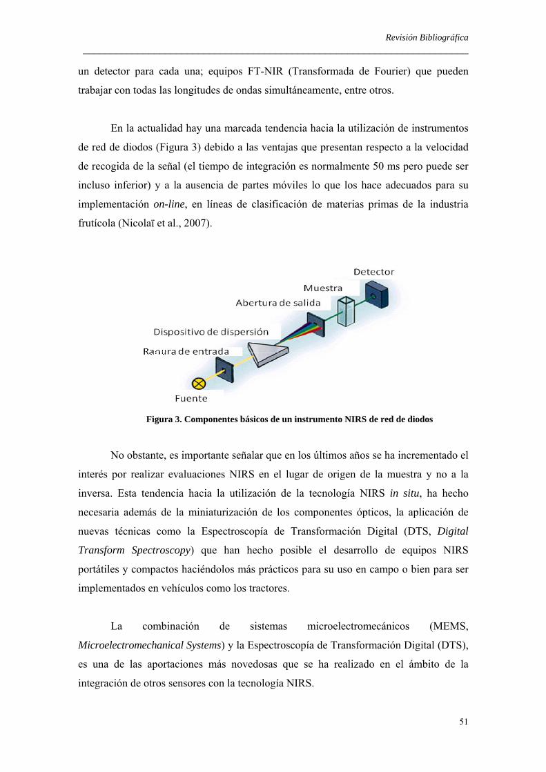
Revisión Bibliográfica ______________________________________________________________________
51
un detector para cada una; equipos FT-NIR (Transformada de Fourier) que pueden
trabajar con todas las longitudes de ondas simultáneamente, entre otros.
En la actualidad hay una marcada tendencia hacia la utilización de instrumentos
de red de diodos (Figura 3) debido a las ventajas que presentan respecto a la velocidad
de recogida de la señal (el tiempo de integración es normalmente 50 ms pero puede ser
incluso inferior) y a la ausencia de partes móviles lo que los hace adecuados para su
implementación on-line, en líneas de clasificación de materias primas de la industria
frutícola (Nicolaï et al., 2007).
Figura 3. Componentes básicos de un instrumento NIRS de red de diodos
No obstante, es importante señalar que en los últimos años se ha incrementado el
interés por realizar evaluaciones NIRS en el lugar de origen de la muestra y no a la
inversa. Esta tendencia hacia la utilización de la tecnología NIRS in situ, ha hecho
necesaria además de la miniaturización de los componentes ópticos, la aplicación de
nuevas técnicas como la Espectroscopía de Transformación Digital (DTS, Digital
Transform Spectroscopy) que han hecho posible el desarrollo de equipos NIRS
portátiles y compactos haciéndolos más prácticos para su uso en campo o bien para ser
implementados en vehículos como los tractores.
La combinación de sistemas microelectromecánicos (MEMS,
Microelectromechanical Systems) y la Espectroscopía de Transformación Digital (DTS),
es una de las aportaciones más novedosas que se ha realizado en el ámbito de la
integración de otros sensores con la tecnología NIRS.

Revisión Bibliográfica ______________________________________________________________________
52
Los sistemas MEMS (Figura 4) están basados en la construcción de dispositivos
fabricados usando tecnología de micro-fabricación a partir de semiconductores,
normalmente silicio, con funciones mecánicas. La superficie de un dispositivo MEMS
consiste en una serie de elementos reflectivos largos, estrechos y programables,
agrupándose cada área del mismo como un píxel.
Figura 4. Componentes básicos de un instrumento NIRS-MEMS
NIRS-MEMS es una tecnología basada en la utilización de un chip o dispositivo
MEMS para la dispersión de los espectros recogidos. Este dispositivo puede ser
controlado de forma que se bloquee la absorción de luz en determinadas regiones del
espectro favoreciendo la absorción/reflectancia en otras partes del espectro. Así,
aplicando un determinado voltaje a los distintos píxeles del dispositivo MEMS es
posible controlar qué píxeles difractarán luz y cuáles la reflejarán en su región espectral
correspondiente, siendo la luz reflejada la que llegará al detector. El escaneo de cada
píxel permitirá la obtención del espectro completo. La luz reflejada por el producto es
entonces recogida por un único detector, siendo ésta una de las mayores ventajas en
cuanto a reducción de costes que presenta la tecnología NIRS-MEMS con respecto a los
equipos de red de diodos (Day et al., 2005), ya que estos últimos, que constituyen la
generación de instrumentos previa a los NIRS-MEMS, incorporan un conjunto de
detectores lo que provoca que sean normalmente fabricados en rangos espectrales de la

Revisión Bibliográfica ______________________________________________________________________
53
zona baja (800-1100 nm) o media (hasta 1700 nm) dentro del infrarrojo cercano, para
poder ser competitivos en coste. Los sensores NIRS-MEMS en cambio al incorporar un
único detector permiten abarcar toda la región del infrarrojo cercano (hasta 2500 nm)
con inferiores costes de producción (Coates y Ramani, 2006).
A pesar de la existencia en el mercado de algunos equipos de diseño manual y
alta portabilidad, la información científica disponible sobre aplicaciones NIRS-MEMS
en el sector agroalimentario es muy limitada. En el ámbito hortofrutícola el primero de
estos trabajos fue publicado en el año 2009, y mostraba la capacidad del equipo manual
PhazirTM (Polychromix, Inc., Wilmington, MA, EE.UU.) (Figura 5) para determinar de
forma no destructiva ciertos parámetros cuantitativos de nectarinas durante su
maduración en árbol y almacenamiento poscosecha (Pérez-Marín et al., 2009).
Posteriormente, en el año 2010 se publicó un segundo trabajo con este tipo de
instrumento destinado a la determinación de la vida útil poscosecha de ciruelas (Pérez-
Marín et al., 2010). En el año 2011, dicha tecnología e instrumento han sido empleados
de nuevo para el control de calidad en árbol y poscosecha de nectarinas cultivadas en
distintos regímenes hídricos (Pérez-Marín et al., 2011; Sánchez et al., 2011), siendo
posteriormente utilizado en la determinaciones de calidad poscosecha de fresas
(Sánchez et al., 2011).
Figura 5. Instrumento portátil NIR-MEMS PhazirTM

Revisión Bibliográfica ______________________________________________________________________
54
Desde un punto de vista de control de procesos, estas dos últimas modalidades
de análisis (redes de diodos y MEMS) son las más interesantes para tomar decisiones en
un reducido margen de tiempo que permitan controlar tanto la calidad del producto final
como la eficiencia del proceso productivo (Pérez-Marín et al., 2009).
3.6.3. Análisis quimiométrico de datos espectroscópicos NIRS.
Un gran avance en la aplicación de las técnicas espectroscópicas para el análisis
de los alimentos y otras materias primas tiene su origen en el desarrollo de algoritmos
matemáticos para el procesado de la información espectral. Estos métodos de análisis de
datos permiten la extracción de información valiosa de grandes y complejos conjuntos
de datos y respaldar la aplicación de la espectroscopía de infrarrojo en muchos campos
de análisis (Martens, 1999; Smyth, 2005; Woodcock et al., 2008; Karoui et al., 2010).
La tecnología NIRS supone una rápida adquisición de gran cantidad de datos
que se deben evaluar e interpretar para transformarlos en información útil. La
quimiometría, disciplina que tiene esta finalidad, contempla todos aquellos procesos que
transforman señales analíticas y datos complejos en información. Para ello utiliza
métodos de origen matemático, estadístico y otros procedentes del campo de la lógica
formal para conseguir sus fines, por lo que se sitúa en un campo interdisciplinar (Casale
et al., 2010).
La Espectroscopía NIR es una técnica ampliamente usada como método de
análisis cuantitativo y cualitativo, para lo cual es necesario el desarrollo de modelos de
predicción.
El modelo de predicción NIRS relaciona la información espectral de las
muestras que constituyen el colectivo de aprendizaje con sus valores para el parámetro
en estudio, proporcionados por un método de referencia. Una vez desarrollado el
modelo, éste permite predecir el contenido de otras muestras de características similares
a las incluidas en el grupo de entrenamiento o calibración.
Para extraer la información química relevante de cada muestra es necesario
recurrir al uso de pretratamientos de la señal espectral, que permiten separar la

Revisión Bibliográfica ______________________________________________________________________
55
información meramente química de las variaciones de origen físico (textura, tamaño,
geometría de las partículas, etc.).
En las señales obtenidas en espectroscopía existen normalmente componentes o
efectos no deseados, también conocidos como ruidos. Estos tienen diferentes orígenes o
causas y afectan de distinta forma al espectro. Los componentes de la instrumentación
utilizados para el registro del espectro (ruido instrumental), las variaciones de
temperatura, humedad u otras condiciones ambientales durante el registro (ruido
ambiental) o bien las variaciones en la señal debidas a la propia naturaleza de la
muestra, pueden ser algunas de las causas del ruido. Otra de las finalidades de los
pretratamientos espectrales es corregir o reducir este ruido.
Los pretratamientos más tradicionalmente utilizados son la derivación, y los
tratamientos de corrección del efecto “scatter” o radiación dispersa denominados
corrección multiplicativa del efecto del scatter, Standard Normal Variate (SNV) y
Detrend (DT) (Shenk y Westerhaus, 1995a; Heise y Winzen, 2002; Naes et al., 2002;
Nicolaï et al., 2007).
Es un hecho que con normalidad se combinen varios métodos de pretratamiento
espectral para eliminar en mayor cuantía el ruido espectral y mejorar así la calidad de
los resultados. Combinaciones de SNV-DT ó DT-SNV y su combinación con derivadas
son habituales.
Es aconsejable realizar estudios previos antes de aplicar las técnicas de
preprocesado de la señal espectral, ya que con ello se elimina una fracción de la
información almacenada, y determinar así la estrategia más adecuada para el colectivo
de muestras o si es necesario aplicar más de un pretratamiento para llevar a cabo la
corrección de datos.
Después de los pretratamientos de la señal espectral, los siguientes pasos están
orientados a desarrollar una ecuación de calibración capaz de predecir parámetros de
calidad de otras muestras con características similares a las incluidas en el colectivo de
aprendizaje (Shenk y Westerhaus, 1995b, 1996; Williams y Sobering, 1996).

Revisión Bibliográfica ______________________________________________________________________
56
3.6.3.1. Análisis de Componentes Principales (ACP)
Uno de los métodos más utilizados y que es recomendable aplicar como etapa
inicial de cualquier análisis multivariante para estudiar la población de muestras con la
que se va a trabajar es el Análisis de Componentes Principales (ACP). Con este
algoritmo se consigue sintetizar la información espectral, detectar muestras anómalas,
obtener información sobre las variables (longitudes de onda) más importantes e
indicaciones sobre el tipo de modelo es más adecuado para ese colectivo de muestras.
La finalidad es desarrollar un modelo bilineal donde los valores de absorbancia
NIR sean las variables originales, las cuales se combinan para formar otras
denominadas Componentes Principales (CP´s) (Jackson, 1991).
El objetivo del ACP es hallar las direcciones que explican la máxima
variabilidad de las muestras y utilizarlas como nuevos ejes de coordenadas, llamados
componentes principales (CP´s). De esta forma, se reduce la dimensionalidad de un
espacio de “k” dimensiones a un espacio de “a” dimensiones (a < k), manteniendo
intacta la información relevante del sistema. Cada componente principal contiene
información de diferente relevancia, describiendo la fuente de variación más importante
de los datos.
Los algoritmos CENTER y SELECT, incluidos en el software WINISI,
(Infrasoft Internacional, Port Matilda, PA, EE.UU.) permiten el estudio de la estructura
y variabilidad espectral de la población de muestras y la selección de muestras que
constituirán el colectivo de calibración. Dichos algoritmos se basan en la realización de
un análisis de componentes principales (ACP), seguido del cálculo de distancias entre
los espectros de las distintas muestras en un espacio n-dimensional, a través
generalmente de la distancia de Mahalanobis (Shenk y Westerhaus, 1995b, 1996). Al
mismo tiempo, estos procedimientos permiten detectar aquellas muestras con
comportamiento diferente, denominadas “anómalas” (outliers), cuya anomalía puede ser
causada tanto por la información espectroscópica o físico-química.

Revisión Bibliográfica ______________________________________________________________________
57
Williams y Norris (2001) realizan una detallada descripción de las posibles
causas de los espectros anómalos; así mismo, señalan que la detección, interpretación y
posible eliminación de estas muestras anómalas es una etapa crítica en el desarrollo de
modelos de predicción, debido a la gran influencia que provoca su presencia en los
resultados del mismo.
Estos procedimientos previos se realizan para definir el colectivo de calibración,
ya sea para la construcción de ecuaciones de calibración (análisis cuantitativo) como
para modelos de clasificación (análisis cualitativo).
3.6.3.2 Análisis cuantitativo. Calibración multivariante
Según Geladi (2003) la aplicación más exitosa de la combinación de la
quimiometría con datos espectrales es el desarrollo de modelos de calibración
multivariantes. En el caso de modelos cuantitativos, se desea utilizar la información
espectral para determinar la concentración de uno o varios componentes o parámetros
en una muestra del producto analizado. Cuando se trabaja con información NIRS, es
fundamental el uso de métodos multivariantes para poder relacionar la información de
múltiples variables con el parámetro o parámetros de interés.
La mayoría de las técnicas matemáticas aplicadas para el desarrollo de
calibraciones se basan en métodos lineales de ajuste, aunque también existen algoritmos
no lineales.
Los métodos lineales obtienen una relación lineal entre la señal espectral y la
concentración de cada componente de interés que se quiere determinar de la muestra.
Esto se basa en asumir que la relación entre la absorbancia y la concentración del
analito establecida por la ley de Lambert-Beer es lineal.
Para el desarrollo de una calibración existen diferentes métodos de regresión
lineal (Martens y Naes, 1989; Burns y Ciurczak, 1992, 2001), siendo los más utilizados
en las aplicaciones cuantitativas NIRS la Regresión Lineal Múltiple (RLM ó MLR), la
Regresión por Componentes Principales (RCP ó PCR), la Regresión mediante Mínimos
Cuadrados Parciales (RMCP ó PLS) y la Regresión mediante Mínimos Cuadrados

Revisión Bibliográfica ______________________________________________________________________
58
Parciales Modificada (RMCPM ó MPLS), siendo éstas dos últimas las más empleadas
en aplicaciones agroalimentarias (Shenk y Westerhaus, 1995b, Pérez-Marín et al.,
2007).
La regresión lineal múltiple utiliza en su totalidad las longitudes de onda del
espectro para realizar el ajuste del modelo, seleccionando algunas variables espectrales
del espectro NIR completo. Las longitudes de onda seleccionadas son aquellas que
presentan una correlación más elevada entre el valor de absorbancia a una longitud de
onda determinada y el dato de referencia correspondiente (Martens y Naes, 1989;
Workman, 1992).
La regresión en componentes principales realiza una reducción de las variables
originales utilizando las componentes principales calculadas mediante un análisis ACP.
Con las nuevas variables ortogonales entre sí realiza un ajuste de regresión múltiple.
Este algoritmo solo usa la información espectral para calcular las nuevas variables, por
lo que éstas son las que mejor representan la matriz de datos, pero no necesariamente
son las más adecuadas para estimar los parámetros de interés a predecir (Massart et al.,
1998).
La regresión de mínimos cuadrados parciales (PLS) parte de la premisa de que la
información espectral es función de unas pocas variables linealmente independientes,
teniendo en cuenta para el cálculo de dichas variables no solo la información espectral
sino además el valor de referencia del parámetro medido para cada muestra (Westerhaus
et al., 2004).
Tanto, la regresión en componentes principales como la regresión en mínimos
cuadrados parciales son métodos de calibración que trabajan con el espectro completo,
aunque sintetizando el mismo en una serie de variables linealmente independientes para
evitar la colinealidad de los datos (Shenk y Westerhaus, 1995a). El uso de estas técnicas
presenta, entre otras muchas, la ventaja de no tener que seleccionar las longitudes de
onda con las que se desarrolla el modelo, si bien su empleo dificulta la interpretación
química de las mismas (Mark y Workman, 1991; Workman, 1992).

Revisión Bibliográfica ______________________________________________________________________
59
La regresión MPLS es una variante de la regresión PLS, cada cual para cada
longitud de onda, los residuos obtenidos después del cálculo de un término, son
estandarizados (divididos por la desviación estándar de los residuales a dicha longitud)
antes de calcular el término siguiente (Shenk y Westerhaus, 1995a). Según indican
Shenk y Westerhaus (1995a) este método es a menudo más preciso y estable que el
algoritmo PLS para productos agroalimentarios, siendo el número de factores de la
regresión seleccionado por validación cruzada (Shenk y Westerhaus, 1995a).
La validación cruzada es un algoritmo que selecciona diferentes colectivos de
calibración y validación dentro de una población específica. El procedimiento consiste
en dividir el colectivo de calibración en grupos (dependiendo del número de muestras).
Cada grupo de validación es predicho una vez con la ecuación desarrollada a partir del
resto de grupos. Este procedimiento además previene el sobreajuste del modelo (Shenk
y Westerhaus, 1995a; Williams, 2001). Los errores de la misma son evaluados mediante
el estadístico Error Típico de Validación Cruzada (ETVC) que es similar al Error Típico
de Predicción (ETP) (Shenk y Westerhaus, 1995a; Williams, 2001).
El ET o error típico, estima la capacidad predictiva del modelo para un colectivo
de muestras nuevas, es el más habitual. Normalmente en la construcción de un modelo
quimiométrico se utiliza un colectivo de calibración, en el que el ET será de calibración
(ETC) y uno de validación externa, en el que el ET será de predicción (ETP).
El error típico de calibración (ETC) que se define como la desviación típica de
los residuales (diferencia entre el valor aportado por el método de referencia y el valor
estimado por la ecuación) para el colectivo de calibración (Williams, 2001). Sin
embargo, suele sobreestimar la capacidad real de predicción de una ecuación al ser
únicamente un estimador del error del modelo quimiométrico empleado (Mark y
Workman, 1991; Shenk y Westerhaus, 1995b).
El error típico de predicción (ETP) es conocido como la desviación típica de las
diferencias, para un colectivo de validación, entre el valor determinado mediante el
método de referencia y el valor estimado mediante el análisis NIRS y es el estadístico
más empleado para estimar la capacidad de predicción de una ecuación de calibración

Revisión Bibliográfica ______________________________________________________________________
60
NIRS (Mark y Workman, 1991; Shenk y Westerhaus, 1995b; Williams, 2001; Wise et
al., 2006).
Asimismo, el estadístico RPD (Ratio of standard error of performance to
standard deviation) que mide la relación entre la desviación típica del colectivo muestral
de calibración y el ETCV y el estadístico RER (Ratio of standard error of performance
to range of standard data), que establece la relación entre el rango de los datos de
referencia de un determinado constituyente y el ETVC para el colectivo de validación
cruzada, son estadísticos muy útiles usados en la evaluación de aplicaciones NIRS
(Williams, 2001).
Según Williams (2001) considera que el RPD es un estadístico sencillo y que
permite la evaluación del ETVC o del ETP en términos de la desviación típica de los
datos de referencia para la población en estudio. De hecho, la eficiencia del análisis
NIRS viene definida por la consistencia de las desviaciones de los datos predichos con
respecto a los datos de referencia, esto es, el ETP o ETVC. Por tanto, si ETP o ETVC
son similares a la desviación típica (o incluso superiores), significaría que la calibración
no estaría prediciendo los valores correctamente. Estos estadísticos deben ser inferiores
a la desviación típica. Williams (2001) señala que valores del RPD comprendidos entre
3 y 5 indican predicciones NIRS eficientes.
El significado de algunos valores de los estadísticos RPD y RER en relación con
la aplicación de la tecnología NIRS en el control de productos y procesos en la Tabla 1.

Revisión Bibliográfica ______________________________________________________________________
61
Tabla 1. Valores de los estadísticos de RPD y RER relacionados con el control NIRS de productos y
procesos
RPD RER Clasificación Aplicación
0,0 – 2,3 < 6 Muy pobre No recomendada
2,4 – 3,0 7 – 12 Pobre Clasificación grosera
3,1 – 4,9 13 – 20 Pasable Clasificación
5,0 – 6,4 21 – 30 Bueno Control de calidad
6,5 – 8,0 31 – 40 Muy bueno Control de procesos
> 8,1 > 41 Excelente Cualquier aplicación
Fuente: Williams, 2001.
El estadístico RER, anteriormente definido es otra forma de estandarizar el ETP
y el ETVC. El valor del RER debería ser tan alto como fuera posible, pero puede ser
aumentado de forma ficticia por una presencia de muestras extremas en concentración
lo cual le resta utilidad y consistencia. Esto no ocurre cuando para estandarizar el ETP o
ETVC utilizamos la desviación típica, es decir, utilizando el RPD.
El coeficiente de variación (CV) que relaciona la desviación típica con la media,
es otro estadístico de uso tradicional en química analítica y de utilidad para la
interpretación de datos NIRS. El tamaño e interpretación del CV depende parcialmente
de la fuente de los datos, es decir, de que se trate de datos de vía húmeda, datos
predichos NIRS, datos de parámetros “funcionales” como dureza, digestibilidad, etc.,
(Williams, 2001). La interpretación del coeficiente de variación en relación con la
aplicación de la tecnología NIRS para el control de productos y procesos se puede
realizar en base a varios criterios (Tabla 2).
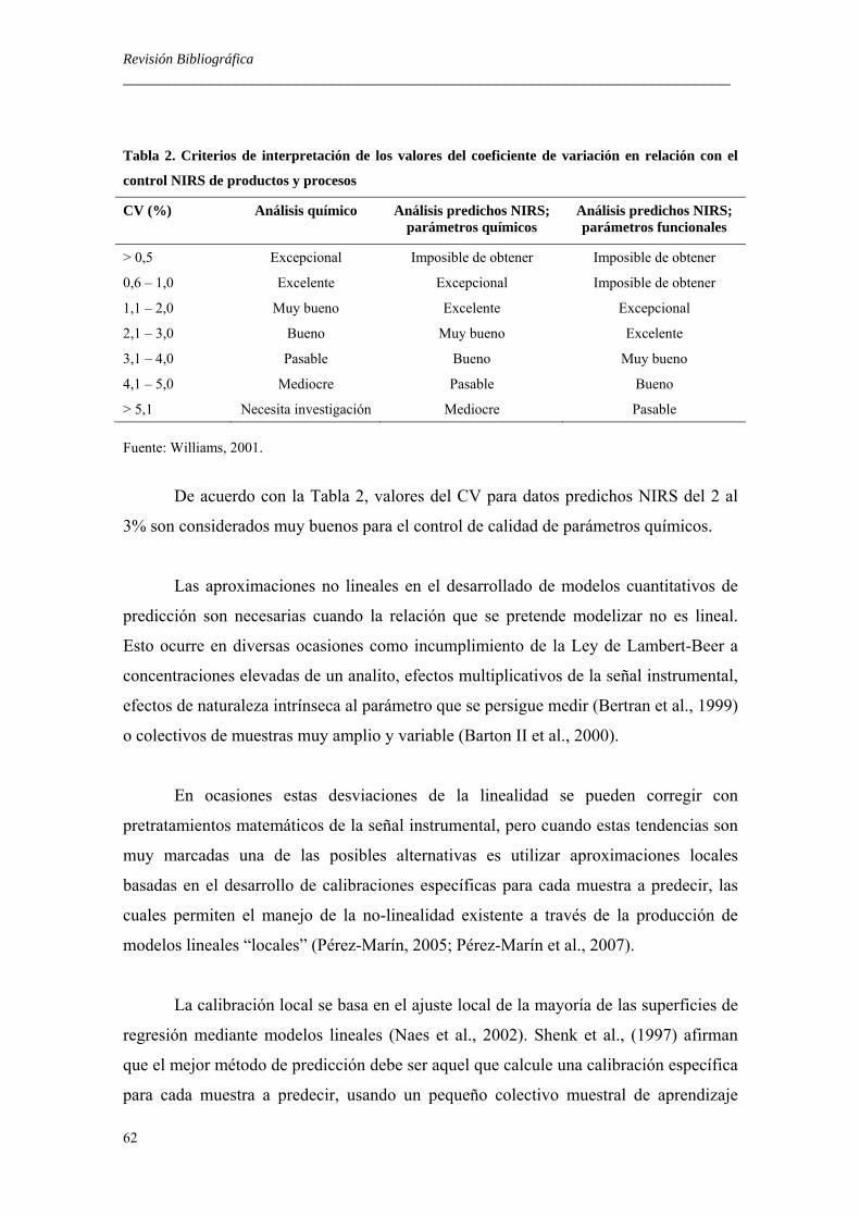
Revisión Bibliográfica ______________________________________________________________________
62
Tabla 2. Criterios de interpretación de los valores del coeficiente de variación en relación con el
control NIRS de productos y procesos
CV (%) Análisis químico
Análisis predichos NIRS; parámetros químicos
Análisis predichos NIRS; parámetros funcionales
> 0,5 Excepcional Imposible de obtener Imposible de obtener
0,6 – 1,0 Excelente Excepcional Imposible de obtener
1,1 – 2,0 Muy bueno Excelente Excepcional
2,1 – 3,0 Bueno Muy bueno Excelente
3,1 – 4,0 Pasable Bueno Muy bueno
4,1 – 5,0 Mediocre Pasable Bueno
> 5,1 Necesita investigación Mediocre Pasable
Fuente: Williams, 2001.
De acuerdo con la Tabla 2, valores del CV para datos predichos NIRS del 2 al
3% son considerados muy buenos para el control de calidad de parámetros químicos.
Las aproximaciones no lineales en el desarrollado de modelos cuantitativos de
predicción son necesarias cuando la relación que se pretende modelizar no es lineal.
Esto ocurre en diversas ocasiones como incumplimiento de la Ley de Lambert-Beer a
concentraciones elevadas de un analito, efectos multiplicativos de la señal instrumental,
efectos de naturaleza intrínseca al parámetro que se persigue medir (Bertran et al., 1999)
o colectivos de muestras muy amplio y variable (Barton II et al., 2000).
En ocasiones estas desviaciones de la linealidad se pueden corregir con
pretratamientos matemáticos de la señal instrumental, pero cuando estas tendencias son
muy marcadas una de las posibles alternativas es utilizar aproximaciones locales
basadas en el desarrollo de calibraciones específicas para cada muestra a predecir, las
cuales permiten el manejo de la no-linealidad existente a través de la producción de
modelos lineales “locales” (Pérez-Marín, 2005; Pérez-Marín et al., 2007).
La calibración local se basa en el ajuste local de la mayoría de las superficies de
regresión mediante modelos lineales (Naes et al., 2002). Shenk et al., (1997) afirman
que el mejor método de predicción debe ser aquel que calcule una calibración específica
para cada muestra a predecir, usando un pequeño colectivo muestral de aprendizaje

Revisión Bibliográfica ______________________________________________________________________
63
constituido por muestras semejantes a la desconocida, seleccionadas dentro de una
amplia biblioteca.
Con la calibración local se consigue modelizar la no-linealidad presente en los
datos, a través de la selección de subgrupos de muestras que presentan rangos de
variabilidad para el parámetro analizado más restringidos, para los que la aplicación de
técnicas de regresión lineales si es adecuada. Además pueden aprovechar la falta de
homogeneidad de las muestras de la librería muestral de partida, usando información
espectral para la selección de colectivos de calibración local que, por ejemplo, tengan
similares tamaños de partícula o similares contenidos en humedad que la muestra
desconocidas que se quiere predecir.
Dentro del marco de definición general de los fundamentos de la calibración
local existen una amplia variación entre los distintos métodos propuestos, tanto en
forma de seleccionar el colectivo de calibración a usar, como en la forma de llevar a
cabo la regresión posterior (Anderssern et al., 2003; Fearn y Davies, 2003).
Entre los tipos de aproximaciones locales que se describen en la literatura, el
algoritmo LOCAL patentado por Shenk y Westerhaus (1998), es uno de los que han
sido más ampliamente utilizado en aplicaciones NIRS.
Shenk et al., (2001) indican que el uso del algoritmo LOCAL puede mejorar la
capacidad predictiva de un modelo obtenido mediante la estrategia de calibración global
entre un 10% y un 30%, dependiendo de la diversidad espectral de las muestras
contenidas en la biblioteca muestral. El algoritmo LOCAL permite una mayor rapidez
en las predicciones (requiere de 1 a 2 segundos por muestra), lo que hace posible su
implementación en el análisis de rutina de un laboratorio cualquiera (Shenk et al.,
1997), siendo el único de los métodos de regresión local que esta incorporado en un
programa comercial (WINISI, Infrasoft Internacional, Port Matilda, PA, EE.UU.).
3.6.3.3. Análisis cualitativo
Aunque la forma más generalizada de aplicación de la tecnología NIRS en
productos agroalimentarios se refiere a determinaciones de carácter cuantitativo, son

Revisión Bibliográfica ______________________________________________________________________
64
muchas las aplicaciones en las que el análisis cualitativo podría estar indicado, habiendo
sido aplicado con éxito en distintos productos agroalimentarios (Le Moigne et al., 2008;
Liu et al., 2008; Zhang et al., 2011; Bao et al., 2012; Mladenov et al., 2012).
El análisis cualitativo NIRS se fundamenta en las características espectrales de
las muestras y consiste en el desarrollo de modelos de clasificación atendiendo a esas
características; se agrupan las muestras con espectros similares, separándolas de otras
con espectros distintos (Downey, 1994, 1996). Este hecho amplia las aplicaciones de
NIRS en el control de calidad de productos agroalimentarios hacia la identificación de
muestras desconocidas, distinción entre variedades, autentificación de productos,
clasificación por calidades, etc. (Paz et al., 2009a y b; Sánchez et al., 2009).
La mayoría de los métodos de análisis cualitativo se basan en medidas de
similitud entre las características espectrales de unas muestras y otras. Dicha similitud
se puede expresar en base a diferentes herramientas tales como correlación espectral,
operaciones lógicas o cálculo de distancias (Pérez-Marín, 2005).
Dentro del análisis cualitativo NIRS se pueden distinguir principalmente tres
aproximaciones (Penchev et al., 1999; Kramer et al., 2004). La primera de ellas hace
referencia al análisis discriminante, en el que varios algoritmos son utilizados para
determinar si una muestra pertenece a un grupo de muestras conocidas a través de
comparaciones espectrales. En segundo lugar, se habla de métodos de reconocimiento
de pautas, usados para determinar el grado de similitud entre el espectro de una muestra
desconocida y una biblioteca espectral. Finalmente, la tercera de las estrategias se
refiere a la interpretación espectral mediante asignación de bandas características.
A su vez, todos los métodos de clasificación se pueden agrupar en dos
categorías, supervisados y no supervisados, dependiendo de si es conocida o no a priori
la asignación de clases del colectivo de aprendizaje (Vandeginste et al., 1998; Heise y
Winzen, 2002; Naes et al., 2002).
Los métodos no supervisados se usan generalmente cuando no se dispone de
información previa del colectivo, pues no se requiere de ningún conocimiento previo de

Revisión Bibliográfica ______________________________________________________________________
65
los objetos para realizar su agrupamiento o clasificación, sino que ellos mismos definen
las clases. El objetivo de este tipo de técnicas es identificar tendencias dentro de los
colectivos de aprendizaje y construir subgrupos o clases en base a ellas (Naes et al.,
2002). Mientras que en los métodos supervisados sucede lo contrario. Éstos se basan en
el aprendizaje previo del sistema, utilizando colectivos de calibración o entrenamiento
en los que las clases y la pertenencia de las distintas muestras a ellas ya se encuentran
definidas (Vandeginste et al., 1998).
Según Pérez-Marín et al., (2006) dentro los procedimientos no supervisados, el
más común es el análisis “clúster” o análisis de conglomerados, que es una técnica de
clasificación multivariante cuya finalidad es definir las pautas naturales de
agrupamiento dentro de colectivos, de forma que los perfiles de las muestras englobadas
dentro de un mismo grupo son muy similares entre sí (cohesión interna del grupo) y los
de las muestras de grupos diferentes son distintos (aislamiento externo del grupo). Otros
métodos no supervisados son las redes neuronales de Kohonene, los métodos de análisis
factorial, el método MST (Minimal Spanning Tree) e incluso también es considerado
como tal, el análisis de componentes principales (Otto, 1999).
Por otro lado, los métodos supervisados se basan en el aprendizaje previo del
sistema, utilizando colectivos de calibración o entrenamiento en los que las clases y la
pertenencia de las distintas muestras a ellas ya se encuentran definidas (Vandenginste et
al., 1998).
Los pasos a seguir en este tipo de métodos son la selección del colectivo de
aprendizaje que debe estar compuesto por un conjunto de muestras analizadas
espectralmente y cuya clasificación es conocida, selección de las variables de
discriminación, obtención del modelo de clasificación mediante la aplicación de una
regla o algoritmo de clasificación y finalmente, la validación de los modelos de
clasificación (Pérez-Marín, 2005).
Entre los métodos supervisados orientados a la discriminación, los más aplicados
en el ámbito de la Espectroscopía NIR son el análisis discriminante lineal (LDA, Linear
Discriminat Analysis), el análisis discriminante cuadrático (QDA, Quadratic
Discriminant Analysis) y el análisis discriminante mediante regresión. Por su parte, los

Revisión Bibliográfica ______________________________________________________________________
66
métodos supervisados dirigidos al modelado de clases más usualmente aplicados son el
análisis discriminante por analogía de clases por modelos independientes (SIMCA, Soft
Independent Modelling of Class Analogy) y las redes neuronales artificiales (Naes e
Indahl, 1998; Vandeginste et al., 1998; Vigneau et al., 2000; Naes et al., 2002).
Una de las aproximaciones cualitativas más ampliamente utilizadas en
aplicaciones NIRS a productos agroalimentarios es el análisis discriminante mediante
regresión PLS, cuyos principios y procedimientos son idénticos a los usados para el
análisis cuantitativo; con la diferencia que mientras para el análisis cuantitativo se mide
la concentración de compuestos, en el análisis discriminante se utilizan variables
discretas, de pertenencia o no a un determinado grupo (Vigneau et al., 2000; Naes et al.,
2002; Kramer et al., 2004).
El análisis discriminante PLS utiliza un colectivo de entrenamiento para el
desarrollo de modelos de predicción cualitativos que pueda aplicarse posteriormente a la
clasificación de nuevas muestras desconocidas. Dicho modelo persigue correlacionar las
variaciones espectrales (X) con las clases definidas (Y), tratando de maximizar la
covarianza existente entre ambos tipos de variables. En este tipo de aproximación, las
variables Y utilizadas no son variables continuas, como en el caso del análisis
cuantitativo, sino que son variables categóricas artificiales o ficticias (“dummy”),
creadas asignando el valor 0 a la muestra perteneciente a la categoría A y el valor 1 a la
muestra perteneciente a la categoría B (Heise y Winzen, 2002; Naes et al., 2002;
Kramer et al., 2004). Según indican Naes et al., (2002), la elección de los valores 0/1
para las variables ficticias es arbitraria, pudiendo ser considerados asimismo otros pares
de valores como 1/2, 0/100. Downey (2000) sugiere que la elección de los valores de las
variables no es importante siempre y cuando la matriz Y sea centrada y normalizada
antes del análisis. Cuando existen dos clases a discriminar se aplica normalmente el
algoritmo PLS1, ya que existe una única variable independiente que toma para cada
muestra del colectivo de aprendizaje un valor de 0 ó 1. El criterio para la clasificación
de muestras desconocidas en una u otra categoría dependerá de que el valor predicho se
aproxime más a 0 ó a 1, respectivamente. Si existen más de dos clases a discriminar,
sólo se podría usar PLS1 si se fuesen dividiendo las clases en grupos de dos de forma
estratificada; aunque, en tal caso, la opción más apropiada sería el uso del algoritmo de

Revisión Bibliográfica ______________________________________________________________________
67
regresión multivariante PLS2. No obstante, este algoritmo también se puede utilizar
cuando exclusivamente se dispone de dos clases (Naes et al., 2002).
El significado de las variables ficticias cambia ligeramente al aplicar PLS2. En
esta aproximación, la variable independiente se convierte en un vector de clases, de
forma que cada muestra tenga un valor de 1 en la clase a la que pertenece y un valor de
0 para el resto de clases (Vandeginste et al., 1998; Heise y Winzen, 2002; Naes et al.,
2002). Por su parte, para la predicción de muestras desconocidas, se obtiene un valor de
la variable discriminatoria para cada una de las clases establecidas; así, un valor de 1 en
una de las categorías representaría una asignación perfecta a la misma, mientras que un
valor de 0 indicaría la no pertenencia a dicha clase. Para una misma muestra, si los
valores de las variables ficticias usados son 0 y 1, los predichos obtenidos para cada
clase deben sumar 1.
Existen diversos criterios para clasificar muestras desconocidas. Aquellos en que
las muestras desconocidas deben ser asignadas al grupo en el que presenten un mayor
valor predicho de la variable discriminatoria (Naes et al., 2002; Kramer et al., 2004), y
otros en los que el valor medio de las variables discriminatorias puede usarse como
límite discriminatorio (Downey y Boussion, 1996; McElhinney y Downey, 1999; Woo
et al., 1999).
Downey (2000) explica que el uso del valor medio sería de aplicación en el caso
de que las clases estuviesen equilibradas en cuanto a número de muestras, pero
recomienda calcular el límite de discriminación entre clases teniendo en cuenta la
desviación típica de los valores predichos para cada clase.
Murray et al., (2001) describen otra aproximación similar en la que consideran
lo que se denomina factor de incertidumbre para calcular el límite de discriminación.
Esta opción está incorporada en el programa quimiométrico WinISI, en la opción de
análisis discriminante mediante PLS2, y calcula el valor de la “mínima diferencia” para
clasificar las muestras en una determinada categoría como el producto del error de
ajuste del modelo por un factor de incertidumbre, cuyo valor está asociado al estadístico
t de Student para un número de grados de libertad infinito. De esta forma, una muestra
es clasificada de forma incierta en una clase cuando la diferencia entre el valor dado a
Revisión Bibliográfica ______________________________________________________________________
68
esa muestra en su clase y el valor que se le da en la/s otra/s clase/s es inferior al valor de
la mínima diferencia (ISI, 2000).
3.7. APLICACIÓN DE LA TECNOLOGÍA NIRS PARA EL CONTROL DE
CALIDAD Y TRAZABILIDAD EN EL SECTOR VITIVINÍCOLA
Los primeros trabajos analíticos llevados a cabo con NIRS se desarrollaron a
finales de los años sesenta para determinar humedad, proteína y grasa en productos
agrícolas (granos y semillas: Norris y Hart, 1965; carne: Ben-Gera y Norris, 1968a;
soja: Ben-Gera y Norris, 1968b). Posteriormente, su aplicación se ha extendido a la
determinación de un gran número de parámetros en productos agroalimentarios, entre
los que destacan las frutas y hortalizas.
En el caso de frutas como la uva y dada su compleja estructura, las ventajas de
desarrollar métodos instrumentales destinados a describir, cuantificar y monitorizar su
composición, son evidentes. Sin embargo, para ser de utilidad práctica en la industria
vitivinícola, los métodos instrumentales deben ser objetivos, rentables y proporcionar
resultados rápidos y reproducibles en funcionamiento continuo.
Actualmente existentes métodos analíticos tradicionalmente empleados para la
determinación de la composición y la calidad de la uva, el vino y otras bebidas
alcohólicas, los cuales no son adecuados para satisfacer las demandas de gestión de
calidad y trazabilidad en un mercado global, debido a su coste y lento tiempo de
respuesta. Incluso los análisis más sencillos requieren enviar las muestras a un
laboratorio independiente con evidentes retrasos en la obtención de resultados
(Cozzolino et al., 2007). Factores tales como la rapidez y bajo coste del análisis, mínima
preparación de la muestra y el respeto al medioambiente, son de vital importancia para
la sostenibilidad de la industria vitivinícola actual (McClure, 2003; Cozzolino et al.,
2006; Nicolaï et al., 2007).
En los últimos 40 años la espectroscopía NIR se ha convertido en uno de los
métodos más atractivos y utilizados de análisis en productos agroalimentarios, ya que
permite la determinación simultánea, rápida y no destructiva de los principales
Revisión Bibliográfica ______________________________________________________________________
69
parámetros de dichos productos. Además, recientemente se han desarrollados estudios
sobre nuevas aplicaciones NIRS que implican la determinación de componentes
minoritarios en productos vegetales (McClure, 2003; Cozzolino et al., 2006; Nicolaï et
al., 2007).
La información acerca de los constituyentes de la uva, el mosto y el vino, es de
gran utilidad para la toma de decisiones en tiempo real en la industria vitivinícola
permitiendo monitorizar y mejorar la adaptación de los sistemas de producción a los
nuevos cambios. Medidas objetivas de la calidad permiten a los elaboradores alcanzar
niveles superiores de la misma, lo que se traduce en un aumento de beneficios por parte
de la industria enológica (Cozzolino et al., 2011a).
Para mejorar aún más la calidad de sus productos, la industria enológica tiene
una evidente necesidad de técnicas simples, rápidas y baratas que evalúen objetivamente
la calidad de la uva (Gishen et al., 2002; Kennedy, 2002; Francis et al., 2005). La
determinación de las características de la uva que influyen decisivamente en la calidad
final del vino, es un requisito básico para mejorar el viñedo y para la óptima producción
del tipo de vino deseado (Cozzolino et al., 2007).
Por lo tanto, el disponer de una tecnología no destructiva, que sea rápida y
precisa, de bajo coste, no contaminante y que pueda ser aplicada directamente en las
líneas de producción, proporcionando datos en tiempo real, y con posibilidad de
aplicación para caracterizar estándares de calidad de las muestras, es de gran interés y
utilidad en el sector vitivinícola. La tecnología NIRS puede considerarse una candidata
idónea para cumplir este objetivo, ya que reúne ampliamente los requisitos
anteriormente indicados, permitiendo además de forma instantánea que un único
análisis espectral proporcione información de atributos muy diversos (Paz et al., 2008;
González-Caballero et al., 2010).
3.7.1. Determinaciones cuantitativas de los principales parámetros de calidad en
uva utilizando NIRS
El sabor y el aroma del vino está implícitamente condicionado por la uva, la
fermentación y en general, por el proceso de elaboración. Para poder elaborar vinos de
Revisión Bibliográfica ______________________________________________________________________
70
la mejor calidad es necesario conocer la composición de la uva, permitiendo con ello la
selección de las técnicas de fermentación del mosto, así como las posibles mezclas de
mostos más adecuadas para elaborar el vino con las características buscadas por el
enólogo. Asimismo, la determinación de la composición de la uva es fundamental para
determinar correctamente el momento de la vendimia (Gishen y Dambergs, 1998;
Gishen et al., 2002; Dambergs et al., 1999, 2003; Francis et al., 2005; Fadock, 2011).
Durante la maduración de la uva es imprescindible estudiar la evolución de
determinados parámetros como el contenido en sólidos solubles, el pH, y la acidez
titulable. Estos componentes son los responsables del contenido de alcohol, azúcar y
acidez del vino, influyendo decisivamente en sus características organolépticas.
Las Tablas 3 y 4 recogen una revisión de los últimos estudios relacionados con
la determinación de parámetros de calidad en uva at-line, e in situ, empleando la
espectroscopía visible y de infrarrojo cercano (VIS-NIR). En dichas tablas se muestran
la variedad analizada, el tipo de instrumento, la presentación de la muestra y el modo de
interacción radiación-muestra, así como la región del espectro electromagnético
utilizada para el desarrollo de los modelos de predicción desarrollados juntos con los
valores de los estadísticos ETVC/ETP, r2 y RPD.

Revisión Bibliográfica ______________________________________________________________________
71
3.7.1.1. Determinaciones cuantitativas at-line de los principales parámetros de calidad
en uva utilizando NIRS
En la Tabla 3 se muestran las principales aplicaciones de la tecnología NIRS
para la determinación de la calidad de la uva realizadas at-line.
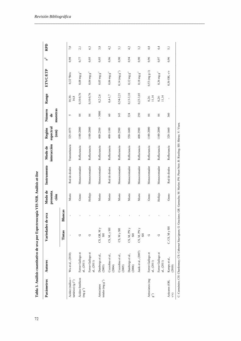
Revisión Bibliográfica ______________________________________________________________________
72
T
abla
3. A
náli
sis
cuan
tita
tivo
de
uva
por
Esp
ectr
osco
pía
VIS
-NIR
. An
ális
is a
t-li
ne
Par
ámet
ros
Au
tore
s V
arie
dad
es d
e u
va
Mod
o de
p
rese
nta
-
ción
Inst
rum
ento
M
odo
de
inte
racc
ión
R
egió
n
esp
ectr
al
(nm
)
Nú
mer
o de
m
ues
tras
Ran
go
ET
VC
/ET
P
r2 R
PD
Tin
tas
Bla
nca
s
Aci
dez
(mál
ico
+
tart
áric
o) (
g l-1
) W
u et
al.,
(20
10)
- -
Mos
to
Red
de
diod
os
Tra
nsm
itanc
ia
325-
1075
5
10,3
0-16
,8
0,32
ºBri
x 0,
98
7,0
Áci
dos
fenó
licos
(m
g g-1
) Fe
rrer
-Gal
lego
et
al.,
(201
1)
G
- G
rano
M
onoc
rom
ador
R
efle
ctan
cia
1100
-200
0 84
0,
10-0
,76
0,08
mg
g-1
0,77
2,
1
Fe
rrer
-Gal
lego
et
al.,
(201
1)
G
- H
olle
jo
Mon
ocro
mad
or
Ref
lect
anci
a 11
00-2
000
84
0,10
-0,7
6 0,
04 m
g g-1
0,
95
6,3
Ant
ocia
nos
tota
les
(mg
g-1)
Dam
berg
s et
al.,
(2
003)
C
S, G
R, M
y
SH
- M
osto
M
onoc
rom
ador
R
efle
ctan
cia
400-
2500
>
300
0 0,
2-2,
6 0,
05 m
g g-1
0,
95
3,8
C
ozzo
lino
et a
l.,
(200
4)
CS,
M, y
SH
-
Mos
to
Red
de
diod
os
Ref
lect
anci
a 40
0-11
00
60
0,4-
1,7
0,06
mg
g-1
0,96
4,
2
C
ozzo
lino
et a
l.,
(200
5)
CS,
M y
SH
-
Mos
to
Mon
ocro
mad
or
Ref
lect
anci
a 40
0-25
00
143
0,54
-2,2
1 0,
14 (
mg
g-1)
0,90
3,
1
D
ambe
rgs
et a
l.,
(200
6)
CS
, M, P
N y
SH
-
Mos
to
Mon
ocro
mad
or
Ref
lect
anci
a 55
0-16
00
324
0,13
-3,1
0 0,
12 m
g g-1
0,
94
4,2
Ja
nik
et a
l., (
2007
) C
S, M
, PN
y
SH
- M
osto
M
onoc
rom
ador
R
efle
ctan
cia
400-
2500
25
0 0,
23-3
,03
0,18
mg
g-1
0,90
3,
2
Ant
ocia
nos
(mg
g-1)
Ferr
er-G
alle
go e
t al
., (2
011)
G
-
Gra
no
Mon
ocro
mad
or
Ref
lect
anci
a 11
00-2
000
84
0,24
-11
,14
0,53
(m
g g-
1)
0,96
4,
8
Fe
rrer
-Gal
lego
et
al.,
(201
1)
G
- H
olle
jo
Mon
ocro
mad
or
Ref
lect
anci
a 11
00-2
000
84
0,24
-11
,14
0,36
mg
g-1
0,97
4,
4
Azú
care
s (O
H,
v/v)
K
emps
et a
l.,
(201
0)
C, C
S, M
y S
H
- G
rano
R
ed d
e di
odos
R
efle
ctan
cia
320-
1660
36
0 -
0,56
OH
, v/v
0,
96
5,1
C: C
arm
énèr
e; C
H: C
hard
onna
y; C
S: C
aber
net S
auvi
gnon
; G: G
raci
ano;
GR
: Gar
nach
a; M
: Mer
lot;
PN
: Pin
ot N
oir;
R: R
iesl
ing;
SH
: Shi
raz;
V: V
iura
.

Revisión Bibliográfica ______________________________________________________________________
73
Tab
la 3
. Aná
lisi
s cu
anti
tati
vo d
e uv
a po
r E
spec
tros
copí
a V
IS-N
IR. A
nális
is a
t-li
ne
(Con
tinu
ació
n)
Par
ámet
ros
Au
tore
s V
arie
dad
es d
e u
va
Mod
o d
e p
rese
nta
-
ción
Inst
rum
ento
M
odo
de
inte
racc
ión
R
egió
n es
pect
ral
(nm
)
Nú
mer
o d
e m
ues
tras
Ran
go
ET
VC
/ET
P
r2 R
PD
Tin
tas
Bla
ncas
Azu
fre
(mg
kg
-1)
Coz
zolin
o et
al.,
(2
011b
) C
S, M
, PN
y
SH
CH
G
rano
ho
mog
enei
zado
M
onoc
rom
ador
R
efle
ctan
cia
400-
2500
20
9 84
,4-2
80,0
- 14
,45
mg
kg-1
0,
88
2,4
Cal
cio
(mg
kg
-1)
Coz
zolin
o et
al.,
(2
011b
) C
S, M
, PN
y
SH
CH
G
rano
ho
mog
enei
zado
M
onoc
rom
ador
R
efle
ctan
cia
400-
2500
20
9 14
5,6-
580,
0 60
,89
mg
kg-1
0,
75
1,5
Com
pues
tos
fenó
licos
to
tale
s (m
g g-1
)
Fer
rer-
Gal
lego
et
al.,
(201
1)
G
- G
rano
M
onoc
rom
ador
R
efle
ctan
cia
1100
-200
0 84
1,
95-1
8,35
0,
59 m
g g-1
0,
98
7,9
F
erre
r-G
alle
go e
t al
., (2
011)
G
-
Hol
lejo
M
onoc
rom
ador
R
efle
ctan
cia
1100
-200
0 84
1,
95-1
8,35
0,
62 m
g g-1
0,
98
7,5
Com
pues
tos
glic
osila
dos
(μM
)
Cyn
kar
et a
l.,
(200
9)
- C
H y
R
Gra
no
hom
ogen
eiza
do
Mon
ocro
mad
or
Ref
lect
anci
a 40
0-25
00
13
333,
5-73
4,0
- -
-
Con
duct
ivid
ad
eléc
tric
a (m
S)
Coz
zolin
o et
al.,
(2
011b
) C
S, M
, PN
y
SH
CH
G
rano
ho
mog
enei
zado
M
onoc
rom
ador
R
efle
ctan
cia
400-
2500
20
9 15
7,0-
256,
0 7,
66 m
g kg
-1
0,87
2,
0
Den
sida
d (g
l-1)
Kem
ps e
t al.,
(2
010)
C
, CS,
M y
SH
-
Gra
no
Red
de
diod
os
Ref
lect
anci
a 32
0-16
60
360
- 12
2 g
l-1
0,96
4,
9
Feno
les
tota
les
(ua)
C
ynka
r et
al.,
(2
009)
-
CH
y R
G
rano
ho
mog
enei
zado
M
onoc
rom
ador
R
efle
ctan
cia
400-
2500
13
25
,6-3
5,2
4,1
ua
4,84
-
Flav
anol
es (
mg
g-1)
Fer
rer-
Gal
lego
et
al.,
(201
1)
G
- G
rano
M
onoc
rom
ador
R
efle
ctan
cia
1100
-200
0 84
0,
41-6
,92
0,35
mg
g-1
0,97
5,
8
F
erre
r-G
alle
go e
t al
., (2
011)
G
-
Hol
lejo
M
onoc
rom
ador
R
efle
ctan
cia
1100
-200
0 84
0,
41-6
,92
0,16
mg
g-1
0,99
13
,6
C: C
arm
énèr
e; C
H: C
hard
onna
y; C
S: C
aber
net S
auvi
gnon
; G: G
raci
ano;
GR
: Gar
nach
a; M
: Mer
lot;
PN
: Pin
ot N
oir;
R: R
iesl
ing;
SH
: Shi
raz;
V: V
iura
.

Revisión Bibliográfica ______________________________________________________________________
74
T
abla
3. A
nál
isis
cu
anti
tati
vo d
e u
va p
or E
spec
tros
cop
ía V
IS-N
IR. A
nál
isis
at-
lin
e (C
onti
nu
ació
n)
Par
ámet
ros
Aut
ores
V
arie
dad
es d
e u
va
Mod
o d
e p
rese
nta -
ción
Inst
rum
ento
M
odo
de
inte
racc
ión
R
egió
n
esp
ectr
al
(nm
)
Nú
mer
o de
m
ues
tras
Ran
go
ET
VC
/ET
P
r2 R
PD
Tin
tas
Bla
ncas
Flav
onol
es (
mg
g-1)
Ferr
er-G
alle
go e
t al
., (2
011)
G
-
Gra
no
Mon
ocro
mad
or
Ref
lect
anci
a 11
00-2
000
84
0,54
-1,7
5 0,
08 m
g g-1
0,
94
4,2
Fe
rrer
-Gal
lego
et
al.,
(201
1)
G
- H
olle
jo
Mon
ocro
mad
or
Ref
lect
anci
a 11
00-2
000
84
0,54
-1,7
5 0,
02 m
g g-1
0,
99
12,7
Fósf
oro
(mg
kg-1
) C
ozzo
lino
et a
l.,
(201
1b)
CS,
M, P
N y
SH
C
H
Gra
no
hom
ogen
eiza
do
Mon
ocro
mad
or
Ref
lect
anci
a 40
0-25
00
209
155,
2-49
0,0
40,1
9 m
g kg
-1
0,70
1,
7
Hie
rro
(mg
kg
-1)
Coz
zolin
o et
al.,
(2
011b
) C
S, M
, PN
y
SH
CH
G
rano
ho
mog
enei
zado
M
onoc
rom
ador
R
efle
ctan
cia
400-
2500
20
9 1,
51-1
3,31
1,
49 m
g kg
-1
0,60
1,
5
IPT
(ua
) K
emps
et a
l.,
(201
0)
C, C
S, M
y S
H
- G
rano
R
ed d
e di
odos
R
efle
ctan
cia
320-
1660
36
0 -
3,09
ua
0,29
1,
2
Mag
nesi
o (m
g kg
-1)
Coz
zolin
o et
al.,
(2
011b
) C
S, M
, PN
y
SH
CH
G
rano
ho
mog
enei
zado
M
onoc
rom
ador
R
efle
ctan
cia
400-
2500
20
9 97
,59-
210,
0 12
,93
mg
kg-1
0,
84
2,2
Man
gane
so
(mg
kg-1
) C
ozzo
lino
et a
l.,
(201
1b)
CS,
M, P
N y
SH
C
H
Gra
no
hom
ogen
eiza
do
Mon
ocro
mad
or
Ref
lect
anci
a 40
0-25
00
209
0,27
-6,5
3 0,
41 m
g kg
-1
0,71
1,
6
Mat
eria
sec
a (%
p/p
) C
ozzo
lino
et a
l.,
(200
8)
C, C
S, M
y P
N
- G
rano
M
onoc
rom
ador
R
efle
ctan
cia
400-
2500
31
0 23
,7-3
8,6-
0,
83 %
p/p
0,
92
3,5
pH
Dam
berg
s et
al.,
(2
003)
C
S, G
R, M
y
SH
- M
osto
M
onoc
rom
ador
R
efle
ctan
cia
400-
2500
>
300
0 2,
8-4,
9 0,
11
2,
8
C
ozzo
lino
et a
l.,
(200
4)
CS,
M y
SH
-
Mos
to
Red
de
diod
os
Ref
lect
anci
a 40
0-11
00
60
3,6-
4,3
0,05
0,
92
2,2
C
ozzo
lino
et a
l.,
(200
5)
CS,
M, y
SH
-
Mos
to
Mon
ocro
mad
or
Ref
lect
anci
a 40
0-25
00
143
3,58
-4,2
6 0,
05
0,81
2,
8
C: C
arm
énèr
e; C
H: C
hard
onna
y; C
S: C
aber
net S
auvi
gnon
; G: G
raci
ano;
GR
: Gar
nach
a; M
: Mer
lot;
PN
: Pin
ot N
oir;
R: R
iesl
ing;
SH
: Shi
raz;
V: V
iura
.

Revisión Bibliográfica ______________________________________________________________________
75
Tab
la 3
. An
ális
is c
uan
tita
tivo
de
uva
por
Esp
ectr
osco
pía
VIS
-NIR
. An
ális
is a
t-li
ne
(Con
tin
uac
ión
)
Par
ámet
ros
Aut
ores
V
arie
dad
es d
e u
va
Mod
o d
e p
rese
nta
-
ción
Inst
rum
ento
M
odo
de
inte
racc
ión
R
egió
n
esp
ectr
al
(nm
)
Nú
mer
o d
e m
ues
tras
Ran
go
ET
VC
/ET
P
r2 R
PD
Tin
tas
Bla
nca
s
pH
Dam
berg
s et
al.,
(2
006)
C
S, M
, PN
y
SH
-
Mos
to
Mon
ocro
mad
or
Ref
lect
anci
a 55
0-16
00
276
2,8-
4,90
0,
08
3,
0
C
ynka
r et
al.,
(2
009)
-
CH
y R
G
rano
ho
mog
enei
zado
M
onoc
rom
ador
R
efle
ctan
cia
400-
2500
13
3,
48-3
,97
0,10
0.
004
-
W
u et
al.,
(20
10)
- -
Mos
to
Red
de
diod
os
Tra
nsm
itan
cia
325-
1075
5
1,66
-2,5
3 0,
05
0,97
5,
4
Pot
asio
(m
g kg
-1)
Coz
zoli
no e
t al.,
(2
011b
) C
S, M
, PN
y
SH
C
H
Gra
no
hom
ogen
eiza
do
Mon
ocro
mad
or
Ref
lect
anci
a 40
0-25
00
209
1570
-360
0 28
5,34
mg
kg-1
0,
78
1,7
SS
T (
ºBri
x)
Jare
n et
al.,
(20
01)
GR
V
G
rano
M
onoc
rom
ador
R
efle
ctan
cia
800-
2500
30
14
-28
1,04
-1,5
9 ºB
rix
0,71
-0,
92
-
D
ambe
rgs
et a
l.,
(200
3)
CS
, GR
, M y
S
H
- M
osto
M
onoc
rom
ador
R
efle
ctan
cia
400-
2500
>
300
0 10
,7-3
7,4
1,0
ºBri
x 0,
99
10,3
A
rana
et a
l.,
(200
5)
- C
H y
V
Gra
no
Mon
ocro
mad
or
Ref
lect
anci
a 80
0-25
00
288
15-2
6 1,
27 ºB
rix
0,67
1,
9
C
ozzo
lino
et a
l.,
(200
5)
CS
, M y
SH
-
Mos
to
Mon
ocro
mad
or
Ref
lect
anci
a 40
0-25
00
143
17,5
-27,
5 0,
68 º
Bri
x 0,
94
4,3
D
ambe
rgs
et a
l.,
(200
6)
CS,
M, P
N y
S
H
- M
osto
M
onoc
rom
ador
R
efle
ctan
cia
800-
1600
32
4 10
,7-3
7,4
0,34
ºBri
x 0,
96
8,8
C
ynka
r et
al.,
(2
009)
-
CH
y R
G
rano
ho
mog
enei
zado
M
onoc
rom
ador
R
efle
ctan
cia
400-
2500
13
19
-24
1,12
ºBri
x 0,
14
-
W
u et
al.,
(20
10)
- -
Mos
to
Red
de
diod
os
Tra
nsm
itan
cia
325-
1075
5
10,3
-16,
8 0,
32 ºB
rix
0,98
6,
97
Tan
inos
co
nden
sado
s (m
g g-1
)
Coz
zoli
no e
t al.,
(2
008)
C
, CS
, M y
PN
-
Gra
no
Mon
ocro
mad
or
Ref
lect
anci
a 40
0-25
00
140
2,8-
9,72
0,
46 m
g g-1
0,
86
3,3
C: C
arm
énèr
e; C
H: C
hard
onna
y; C
S: C
aber
net S
auvi
gnon
; G: G
raci
ano;
GR
: Gar
nach
a; M
: Mer
lot;
PN
: Pin
ot N
oir;
R: R
iesl
ing;
SH
: Shi
raz;
V: V
iura
.

Revisión Bibliográfica ______________________________________________________________________
76
El análisis de la Tabla 3 indica que la mayor parte de las determinaciones de
parámetros de calidad en uva realizadas at-line han sido llevadas a cabo empleando
instrumentos monocromadores (Dambergs et al., 2003, 2006; Cozzolino et al., 2005,
2008, 2011b; Janik et al., 2007; Cynkar et al., 2009; Ferrer-Gallego et al., 2011), frente
a los equipos de redes de diodos utilizados por Cozzolino et al., (2004); Kemps et al.,
(2010); Wu et al., (2010).
Asimismo, se puede observar que la mayoría de los trabajos realizados utilizan
la región del visible junto con la región NIR (400-1100 nm y 400-2500 nm), mientras
que son más escasos los trabajos de investigación que utilizan instrumentos que trabajen
exclusivamente en la región NIRS (800-2500 nm y 1100-2000 nm).
Igualmente, el modo de interacción de la muestra con el instrumento en todos los
trabajos realizados ha sido la reflectancia, a excepción de Wu et al., (2010) quienes
utilizan la transmitancia.
Es importante señalar que la mayoría de las modelos NIRS desarrollados para los
distintos parámetros de calidad de uva ensayados han empleado la regresión por
mínimos cuadrados parciales (PLS), método muy extendido para aplicaciones
agroalimentarias en este ámbito, siendo escasos los estudios que utilizan modelos de
regresión no lineal como LOCAL (Dambergs et al., 2003, 2006), máquinas de vectores
soporte (Chauchard et al., 2004), redes neuronales (Janik et al., 2007). Sin embargo,
dichos autores, obtienen modelos más robustos y precisos al emplear técnicas de
regresión no lineales.
Dentro de los parámetros de calidad destinados a la determinación de la
composición de la uva ha sido el contenido en sólidos solubles totales el más estudiado
(Jarén et al., 2001; Dambergs et al., 2003, 2006; Arana et al., 2005; Cozzolino et al.,
2005; Cynkar et al., 2009; Wu et al., 2010). Los valores de los estadísticos obtenidos
por Dambergs (2003, 2006) muestran la excelente capacidad de NIRS para la predicción
de dicho parámetro (RPD = 10,3; r2 = 0,99 y RPD = 8,8; r2 = 0,96, respectivamente),
siendo el análisis del contenido en sólidos solubles totales esencial para la industria

Revisión Bibliográfica ______________________________________________________________________
77
enológica, ya que su determinación establece el grado de madurez del fruto y es una
medida aproximada de la concentración en azúcares del mismo. El conocimiento de este
parámetro permitirá la estimación del contenido alcohólico probable del vino,
favoreciendo la separación de la uva por calidades, lo que posibilitará elaborar vinos de
la mejor calidad.
Los estudios realizados sobre este parámetro utilizan en su mayoría como forma
de presentación de la muestra al instrumento el mosto (Dambergs et al., 2003; 2006;
Cozzolino et al., 2005; Wu et al., 2010) excepto Jarén et al., (2001) y Arana et al.,
(2005) quienes utilizan grano, mientras que Cynkar et al., (2009) es el único que utiliza
grano homogeneizado (trituración del grano obteniendo una pasta homogénea). Todos
los trabajos emplean la región del visible junto con la región NIR (400- 1100 nm y 400-
2500 nm).
El pH también ha sido un parámetro estudiado en diferentes trabajos de
investigación realizados con instrumentos NIRS dispuestos at-line (Dambergs et al.,
2003, 2006; Cozzolino et al., 2004, 2005; Cynkar et al., 2009; Wu et al., 2010). Sin
embargo, los resultados de los estadísticos de los modelos predictivos desarrollados sólo
fueron satisfactorios para Wu et al., (2011) (RPD = 5,4; r2 = 0,97). El resto de los
autores desarrollaron modelos considerados de baja o muy baja capacidad predictiva.
No obstante, la importancia de la determinación del pH es clave en la industria
enológica para llevar a cabo las correcciones necesarias en mostos, así como para la
elaboración de vinos de calidad.
En los trabajos destinados a la determinación de pH se utilizó como forma de
presentación de la muestra al instrumento el mosto, a excepción de Cynkar et al., (2009)
quienes emplean el grano homogeneizado, no utilizándose la presentación en grano en
ninguno de los trabajos realizados.
Recientemente, diversos autores han abordado la determinación del contenido en
antocianos empleando NIRS (Dambergs et al., 2003, 2006; Cozzolino et al., 2004,
2005; Janik et al., 2007; Ferrer-Gallego et al., 2011). Los valores de r2 obtenidos para
este parámetro indican que los modelos desarrollados permiten la clasificación en alta,
media y baja del contenido en antocianos de los frutos analizados (Williams, 2001).
Revisión Bibliográfica ______________________________________________________________________
78
Para la industria enológica, el disponer de datos sobre dicho parámetro es muy
importante ya que los antocianos tienen una influencia directa sobre el contenido
polifenólico de los vinos. La concentración de este parámetro durante la maduración de
la uva, aumenta hasta alcanzar un punto máximo después del cual disminuye
ligeramente, condicionando de forma definitiva la calidad del vino tinto.
Los estudios realizados en antocianos con tecnología NIR utilizan el mosto como
forma de presentación de la muestra al instrumento, a excepción del realizado por
Ferrer-Gallego et al., (2011) quienes utilizan grano y hollejo, empleando la reflectancia
como modo de interacción de la muestra al instrumento. De nuevo el rango espectral
utilizado es el que recoge la región del visible junto con la región NIR (400-1100 nm y
400-2500 nm).
En el último año, se han llevado a cabo el desarrollo de aplicaciones NIRS
destinadas a la determinación en uvas del contenido en ácido málico (Wu et al., 2011) y
azufre, calcio, fósforo, hierro, magnesio, manganeso y conductividad eléctrica
(Cozzolino et al., 2011b).
Así, Wu et al., (2001) utilizando el mosto como forma de presentación de la
muestra al instrumento, obtuvieron excelentes modelos de predicción del contenido en
ácido málico en uvas (RPD = 7, r2 = 0,98), confirmando la viabilidad de NIRS para la
predicción de dicho parámetro. Asimismo, Cozzolino et al., (2011b) utilizando el grano
homogeneizado como forma de presentación, obtienen resultados prometedores para la
predicción del contenido en metales (S, Ca, P, Fe, Mg y Mg) así como para la
determinación de la conductividad eléctrica de la uva.

Revisión Bibliográfica ______________________________________________________________________
79
3.7.1.2. Determinaciones cuantitativas in situ de los principales parámetros de calidad
en uva utilizando NIRS
En la Tabla 4 se muestran las determinaciones in situ de parámetros de calidad
en uva realizadas empleando la tecnología NIRS.

Revisión Bibliográfica ______________________________________________________________________
80
Tab
la 4
. An
ális
is c
uant
itat
ivo
de
uva
por
Esp
ectr
osco
pía
VIS
-NIR
. An
ális
is in
sit
u
Par
ámet
ros
Au
tore
s V
arie
dad
es d
e u
va
Mod
o d
e p
rese
nta
-
ción
Inst
rum
ento
M
odo
de
inte
racc
ión
R
egió
n
esp
ectr
al
(nm
)
Nú
mer
o d
e m
ues
tras
Ran
go
ET
VC
/ET
P
r2 R
PD
Tin
tas
Bla
nca
s
Aci
dez
(mál
ico
+
tart
áric
o) (
g l-1
) C
hauc
hard
et a
l.,
(200
4)
CG
M
V y
UB
G
rano
R
ed d
e di
odos
T
rans
mit
anci
a 68
0-11
00
371
2-16
1,
03 g
l-1
0,86
-
Aci
dez
titu
labl
e (á
cido
tart
áric
o)
(g d
m-3
)
Gui
dett
i et a
l.,
(201
0)
N
- G
rano
R
ed d
e di
odos
R
efle
ctan
cia
400-
1000
71
5,
8-28
,8
1,48
g d
m-3
0,
66
-
G
uide
tti e
t al.,
(2
010)
N
-
Gra
no
hom
ogen
eiza
do
Red
de
diod
os
Ref
lect
anci
a 40
0-10
00
134
5,8-
28,8
1,
12 (
g dm
-3)
0,72
-
Aci
dez
titu
labl
e (á
cido
tart
áric
o)
(g l-1
)
Men
esat
ti, (
2007
) C
S, M
y S
G
- G
rano
R
ed d
e di
odos
R
efle
ctan
cia
Inte
rect
anci
a 40
0-11
00
450
- 0,
2 g
l-1
0,46
-
Ant
ocia
nos
extr
aíbl
es p
H 3
,2
(mg
dm-3
)
Gui
dett
i et a
l.,
(201
0)
N
- G
rano
R
ed d
e di
odos
R
efle
ctan
cia
400-
1000
71
94
,5-
823,
7 81
,87
mg
dm-3
0,45
-
G
uide
tti e
t al.,
(2
010)
N
-
Gra
no
hom
ogen
eiza
do
Red
de
diod
os
Ref
lect
anci
a 40
0-10
00
135
94,5
-82
3,7
77,7
mg
dm-3
0,
71
-
Ant
ocia
nos
pote
ncia
les
pH 1
(m
g dm
-3)
Gui
dett
i et a
l.,
(201
0)
N
- G
rano
R
ed d
e di
odos
R
efle
ctan
cia
400-
1000
71
14
8,1-
1350
13
3,90
mg
dm-3
0,50
-
G
uide
tti e
t al.,
(2
010)
N
-
Gra
no
hom
ogen
eiza
do
Red
de
diod
os
Ref
lect
anci
a 40
0-10
00
137
148,
1-13
50
129
mg
dm-3
0,61
-
C: C
arm
énèr
e; C
G: C
ariñ
ena;
CH
: Cha
rdon
nay;
CS
: Cab
erne
t Sau
vign
on; M
: Mer
lot;
MV
: Mou
rvéd
re; N
: Neb
biol
o; P
N: P
inot
Noi
r; S
G: S
an G
iove
se; U
B: U
gni B
lanc
.
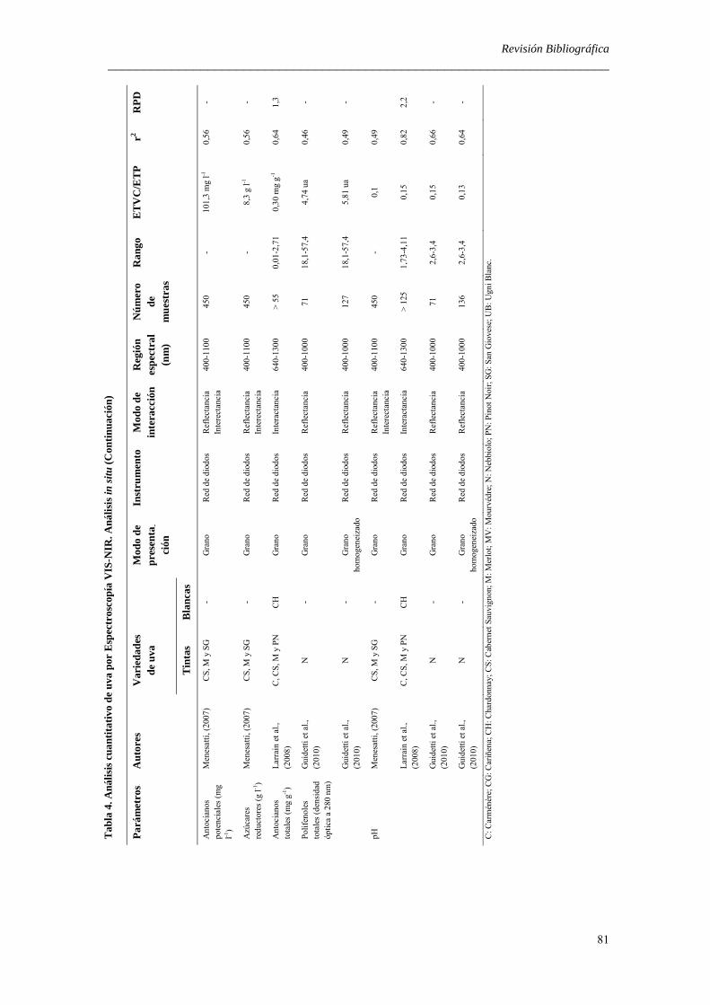
Revisión Bibliográfica ______________________________________________________________________
81
Tab
la 4
. Aná
lisis
cua
ntit
ativ
o de
uva
por
Esp
ectr
osco
pía
VIS
-NIR
. Aná
lisis
in s
itu
(Con
tinu
ació
n)
Par
ámet
ros
Au
tore
s V
arie
dad
es
de u
va
M
odo
de
pre
sen
ta-
ción
Inst
rum
ento
M
odo
de
inte
racc
ión
Reg
ión
esp
ectr
al
(nm
)
Nú
mer
o d
e m
ues
tras
Ran
go
ET
VC
/ET
P
r2 R
PD
Tin
tas
Bla
ncas
Ant
ocia
nos
pote
ncia
les
(mg
l-1)
Men
esat
ti, (
2007
) C
S, M
y S
G
- G
rano
R
ed d
e di
odos
R
efle
ctan
cia
Inte
rect
anci
a 40
0-11
00
450
- 10
1,3
mg
l-1
0,56
-
Azú
care
s re
duct
ores
(g
l-1)
Men
esat
ti, (
2007
) C
S, M
y S
G
- G
rano
R
ed d
e di
odos
R
efle
ctan
cia
Inte
rect
anci
a 40
0-11
00
450
- 8,
3 g
l-1
0,56
-
Ant
ocia
nos
tota
les
(mg
g-1)
Lar
rain
et a
l.,
(200
8)
C, C
S, M
y P
N
CH
G
rano
R
ed d
e di
odos
In
tera
ctan
cia
640-
1300
>
55
0,01
-2,7
1 0,
30 m
g g-1
0,
64
1,3
Polif
enol
es
tota
les
(den
sida
d óp
tica
a 28
0 nm
)
Gui
dett
i et a
l.,
(201
0)
N
- G
rano
R
ed d
e di
odos
R
efle
ctan
cia
400-
1000
71
18
,1-5
7,4
4,74
ua
0,46
-
G
uide
tti e
t al.,
(2
010)
N
-
Gra
no
hom
ogen
eiza
do
Red
de
diod
os
Ref
lect
anci
a 40
0-10
00
127
18,1
-57,
4 5,
81 u
a 0,
49
-
pH
Men
esat
ti, (
2007
) C
S, M
y S
G
- G
rano
R
ed d
e di
odos
R
efle
ctan
cia
Inte
rect
anci
a 40
0-11
00
450
- 0,
1 0,
49
L
arra
in e
t al.,
(2
008)
C
, CS,
M y
PN
C
H
Gra
no
Red
de
diod
os
Inte
ract
anci
a 64
0-13
00
> 1
25
1,73
-4,1
1 0,
15
0,82
2,
2
G
uide
tti e
t al.,
(2
010)
N
-
Gra
no
Red
de
diod
os
Ref
lect
anci
a 40
0-10
00
71
2,6-
3,4
0,15
0,
66
-
G
uide
tti e
t al.,
(2
010)
N
-
Gra
no
hom
ogen
eiza
do
Red
de
diod
os
Ref
lect
anci
a 40
0-10
00
136
2,6-
3,4
0,13
0,
64
-
C: C
arm
énèr
e; C
G: C
ariñ
ena;
CH
: Cha
rdon
nay;
CS:
Cab
erne
t Sau
vign
on; M
: Mer
lot;
MV
: Mou
rvéd
re; N
: Neb
biol
o; P
N: P
inot
Noi
r; S
G: S
an G
iove
se; U
B: U
gni B
lanc
.
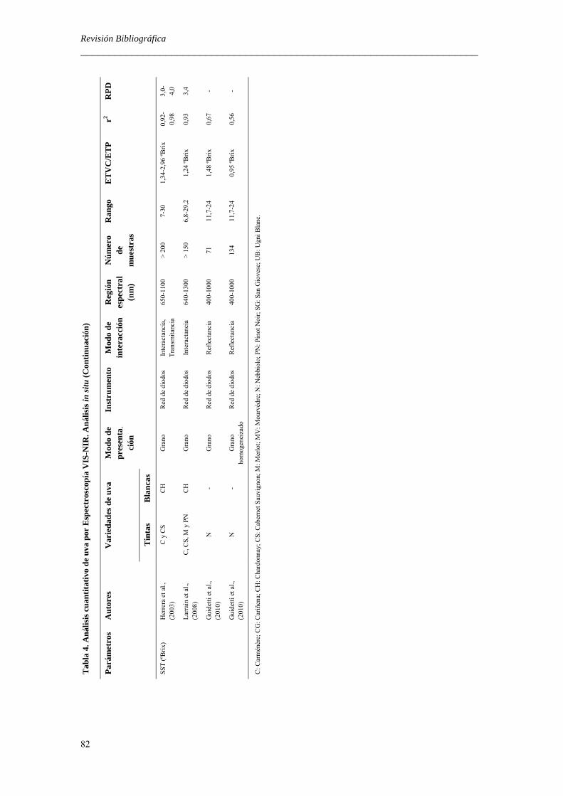
Revisión Bibliográfica ______________________________________________________________________
82
Tab
la 4
. An
ális
is c
uan
tita
tivo
de
uva
por
Esp
ectr
osco
pía
VIS
-NIR
. An
ális
is in
sit
u (
Con
tin
uac
ión
)
Par
ámet
ros
Aut
ores
V
arie
dad
es d
e u
va
Mod
o d
e p
rese
nta
-
ción
Inst
rum
ento
M
odo
de
inte
racc
ión
R
egió
n
esp
ectr
al
(nm
)
Nú
mer
o d
e m
ues
tras
Ran
go
ET
VC
/ET
P
r2 R
PD
Tin
tas
Bla
nca
s
SS
T (
ºBri
x)
Her
rera
et a
l.,
(200
3)
C y
CS
CH
G
rano
R
ed d
e di
odos
In
tera
ctan
cia,
T
rans
mita
ncia
65
0-11
00
> 2
00
7-30
1,
34-2
,96
ºBri
x 0,
92-
0,98
3,
0-4,
0
L
arra
in e
t al.,
(2
008)
C
, CS
, M y
PN
C
H
Gra
no
Red
de
diod
os
Inte
ract
anci
a 64
0-13
00
> 1
50
6,8-
29,2
1,
24 ºB
rix
0,93
3,
4
G
uide
tti e
t al.,
(2
010)
N
-
Gra
no
Red
de
diod
os
Ref
lect
anci
a 40
0-10
00
71
11,7
-24
1,48
ºBri
x 0,
67
-
G
uide
tti e
t al.,
(2
010)
N
-
Gra
no
hom
ogen
eiza
do
Red
de
diod
os
Ref
lect
anci
a 40
0-10
00
134
11,7
-24
0,95
ºBri
x 0,
56
-
C: C
arm
énèr
e; C
G: C
ariñ
ena;
CH
: Cha
rdon
nay;
CS
: Cab
erne
t Sau
vign
on; M
: Mer
lot;
MV
: Mou
rvéd
re; N
: Neb
biol
o; P
N: P
inot
Noi
r; S
G: S
an G
iove
se; U
B: U
gni B
lanc
.

Revisión Bibliográfica ______________________________________________________________________
83
En el caso de determinaciones de calidad de uva realizadas in situ los
instrumentos NIRS empleados son todos ellos de redes de diodos (Herrera et al., 2003;
Chauchard et al., 2004, Menesatti, 2007; Larraín et al., 2008; Guidetti et al., 2010)
(Tabla 4). Dichos autores concluyen que Vis/NIR puede ser una interesante y rápida
herramienta para controlar el seguimiento de maduración o para realizar controles en
recepción en bodega, empleando equipos portátiles.
Todos los trabajos realizados in situ emplean la región del visible junto con la
región NIR (400-1300 nm), siendo la forma de presentación de la muestra al
instrumento en la mayoría de los casos en grano, excepto Guidetti et al., (2010) quienes
también utilizaron en su estudio grano homogeneizado.
En cuanto al modo de interacción de la muestra al instrumento utilizado en
determinaciones in situ se han empleado tanto la reflectancia, la interactancia-
reflectancia como la transmitancia.
Al igual que para las determinaciones at-line, en las determinaciones in-situ de
calidad de la uva, los parámetros más estudiados han sido el contenido en sólidos
solubles totales (Herrera et al., 2003; Larraín et al., 2008; Guidetti et al., 2010) y el pH
(Menesatti, 2007; Larraín et al., 2008; Guidetti et al., 2010).
Los mejores resultados para la determinación del contenido en sólidos solubles
totales han sido los obtenidos por Herrera et al., (2003), con valores de los estadísticos
RPD = 4; r2 = 0,98. En el caso del pH, los mejores modelos fueron los obtenidos por
Larraín et al., (2008) (RPD = 2,2; r2 = 0,82)
Asimismo, la determinación del contenido en antocianos ha sido llevada a cabo
aplicando NIRS in situ (Menesatti, 2007; Larraín et al., 2008; Guidetti et al., 2010),
permitiendo los modelos obtenidos la clasificación de las muestras como de bajo, medio
y alto contenido en antocianos (Williams, 2001).

Revisión Bibliográfica ______________________________________________________________________
84
Por último, señalar que la determinación in situ de parámetros de calidad de uva
mediante NIRS es de gran importancia para la industria enológica, ya que permitiría el
seguimiento de la maduración del fruto en la cepa. El estado de madurez de la uva
condiciona totalmente el vino que se quiere obtener y sus características. Por ello es
necesario realizar estudios de maduración, siguiendo la evolución en la vid de los
componentes de la uva, que aporten información para decidir el momento óptimo de la
vendimia.
3.8. REFLEXIONES FINALES SOBRE EL ESTADO DE DESARROLLO DEL
ANÁLISIS NIRS EN LA INDUSTRIA VITIVINÍCOLA
Como ha sido puesto de manifiesto en la revisión bibliográfica realizada, para la
industria enológica sería muy interesante el disponer de una técnica de análisis no
destructiva, que no requiera preparación alguna de la muestra, respetuosa con el medio
ambiente y fiable destinada a la determinación de parámetros en la uva tales como el
contenido en sólidos solubles totales (SST) y en azúcares reductores, la acidez titulable
y el pH, así como los contenidos en ácidos tartárico, málico y en potasio, con la mayor
precisión y empleando el menor tiempo posible, con el fin de realizar actuaciones
rápidas tanto sobre la materia prima como sobre el mosto, destinadas a determinar el
momento óptimo de cosecha, así como la variedad o la mezcla de variedades más
adecuadas, en función de los parámetros de calidad interna seleccionados, para obtener
un vino de calidad.
El hecho de conocer los principales parámetros de calidad interna de la uva
anteriormente citados, permitiría a la industria enológica el poder realizar las
correcciones necesarias en caso de pH altos y valor de acidez titulable bajos, así como
correcciones en mostos con bajos contenidos en azúcares adicionando mostos
concentrados o mostos concentrados rectificados, estando todas ellas destinadas a
obtener vinos de alta calidad. Sin embargo, los métodos de análisis tradicionales
empleados para la determinación de dichos parámetros resultan ser destructivos y
tediosos.

Revisión Bibliográfica ______________________________________________________________________
85
La tecnología NIRS ofrece importantes posibilidades para abordar las
necesidades analíticas de control y aseguramiento de la calidad de la industria enológica
de forma integral, permitiendo la toma de decisiones en tiempo real. Asimismo, es
importante tener en consideración que el procesado de la muestra y la presentación de la
misma al instrumento son factores importantes en la solidez y la precisión de NIRS
como una técnica analítica.
A pesar de que ciertas investigaciones anteriores han demostrado el potencial de
la tecnología NIRS para la caracterización cuantitativa de los parámetros de calidad de
uva de vinificación, es importante señalar que la inmensa mayoría de los estudios
anteriormente citados han sido realizados empleando uva desgranada, mosto o grano
homogeneizado, lo que implica un cierto pre-procesado del producto previamente a la
presentación del mismo al instrumento, variando la intensidad del mismo en función del
tipo de materia prima utilizado. Hecho que va en detrimento de una de las principales
ventajas del empleo de NIRS como es la nula preparación de la muestra para su análisis.
Igualmente, el desarrollo instrumental acaecido en los últimos años, donde
destacan los instrumentos de redes de diodos sin elementos móviles que ofrecen la
posibilidad de adquirir la información espectral de superficies de muestra relativamente
grandes en un corto período de tiempo y su aplicación para el análisis en línea, en la
recepción en bodega y durante el proceso del elaboración de mostos y vinos, así como el
desarrollo de equipos portátiles de tamaño reducido, de diseño manual y que funcionan
con baterías como los instrumentos NIRS-MEMS, cuyo diseño óptico y ergonomía
abren enormes expectativas para la recogida de datos espectrales in situ antes o durante
la cosecha, permitiendo así la posibilidad de realizar modelos predictivos destinados a
determinar el momento óptimo de la misma, hace necesario el contar con estudios de
comparación de instrumentos destinados a determinar la idoneidad de los mismos en
función de su aplicación en la industria enológica.
Respecto al método multivariante utilizado para el ajuste de los modelos de
predicción, es habitual, para aplicaciones NIRS en uvas y mostos, el empleo de
regresión lineal, tipo PLS, existiendo escasas referencias relativas a la aplicación de
métodos no lineales.
Revisión Bibliográfica ______________________________________________________________________
86
Por lo tanto, se puede afirmar que si bien durante las últimas décadas se ha
producido un incremento de las aplicaciones de NIRS en la industria vitivinícola, el uso
de la Espectroscopía NIR en la industria del vino está todavía en sus comienzos y es
necesario por lo tanto, seguir investigando y optimizar el uso de esta tecnología en el
sector vitivinícola, siendo la realización de medidas sobre racimo uno de los aspectos a
desarrollar. Por todo ello, se planteó la presente Tesis Doctoral con los objetivos que
han sido descritos en el Capítulo 2 del presente documento.

Capítulo 4


NIRS para la predicción de parámetros de calidad interna y momento óptimo de cosecha en uvas y control de calidad y trazabilidad en la industria vitivinícola
______________________________________________________________________
89
Capítulo 4. LA TECNOLOGÍA NIRS PARA LA PREDICCIÓN DE
PARÁMETROS DE CALIDAD INTERNA, DETERMINACIÓN DEL
MOMENTO ÓPTIMO DE COSECHA Y CONTROL DE CALIDAD
Y TRAZABILIDAD EN LA INDUSTRIA VITIVINÍCOLA
4.1. FIRST STEPS TOWARDS THE DEVELOPMENT OF A NON-
DESTRUCTIVE TECHNIQUE FOR THE QUALITY CONTROL OF WINE
GRAPES DURING ON-VINE RIPENING AND ON ARRIVAL AT THE
WINERY. JOURNAL OF FOOD ENGINEERING 101, 158–165 (2010)

90

Journal of Food Engineering 101 (2010) 158–165
Contents lists available at ScienceDirect
Journal of Food Engineering
journal homepage: www.elsevier .com/locate / j foodeng
First steps towards the development of a non-destructive techniquefor the quality control of wine grapes during on-vine ripening and onarrival at the winery
Virginia González-Caballero a, María-Teresa Sánchez b,*, María-Isabel López a, Dolores Pérez-Marín c,**
a Centro de Investigación y Formación Agraria de ‘‘Cabra-Priego”, Instituto de Investigación y Formación Agraria y Pesquera (IFAPA), Consejería de Agricultura y Pesca,Junta de Andalucía, Cabra, Spainb Department of Bromatology and Food Technology, University of Cordoba, Campus of Rabanales, 14071 Cordoba (Cárdoba), Spainc Department of Animal Production, University of Cordoba, Campus Rabanales, 14071 Cordoba, Spain
a r t i c l e i n f o a b s t r a c t
Article history:Received 1 October 2009Received in revised form 22 June 2010Accepted 23 June 2010Available online 24 July 2010
Keywords:NIR spectroscopyGrapesQuality parametersNon-destructive analysisOn-vineBunch analysis
0260-8774/$ - see front matter � 2010 Elsevier Ltd. Adoi:10.1016/j.jfoodeng.2010.06.016
* Corresponding author. Tel.: +34 957 212576; fax:** Corresponding author. Tel.: +34 957 212576; fax:
E-mail addresses: [email protected] (M.-T. S(D. Pérez-Marín).
NIR spectroscopy was used as a non-destructive technique for the assessment of changes in certain inter-nal quality properties of wine grapes (Vitis vinifera L.) during on-vine ripening and at harvest. A total of108 different wine grape samples were used to construct calibration models based on reference data andNIR spectral data, obtained using a commercially-available diode-array spectrophotometer (380–1700 nm). The feasibility of testing bunches of intact grapes was investigated and compared with moretraditional methods of presentation, such as berries or must. Predictive models were constructed toquantify changes in soluble solid content (SSC, �Brix), reducing-sugar content (g/l), pH-value, titrableacidity (g/l tartaric acid), tartaric acid (g/l) and malic acid (g/l), these being the major parameters usedto chart ripening. NIRS technology provided good precision for the bunch analysis mode assayed forSSC (r2 = 0.89; SECV = 1.41 �Brix), for reducing-sugar content (r2 = 0.87; SECV = 17.13 g/l) and for pH-value (r2 = 0.69; SECV = 0.19). Models developed for testing other fruit acidity parameters yielded resultssufficient to provide a screening tool to distinguish between low and high acidity values in intact grapes.Significantly, the results obtained with bunch presentation were similar to those obtained with berriesand must, thus justifying further implementation of NIRS technology for the non-destructive analysisof quality properties both during on-vine ripening and on arrival at the winery. This method allows muststo be processed separately depending on initial grape quality, assessed with a single spectrum measure-ment and in a matter of seconds.
� 2010 Elsevier Ltd. All rights reserved.
1. Introduction
Measurement of certain grape quality parameters – e.g. totalsoluble solid content (SSC), reducing-sugar content, titrable acidity,pH-value, tartaric acid and malic acid content – is essential foroptimum harvest timing and for ensuring the production of high-quality wines that are both chemically and biologically stable(Martínez-Toda, 2007).
However, traditional analytical methods applied to the mea-surement of these parameters in grapes and wines have provedto be slow, tedious and destructive, and do not match the demandsof modern wine production in a global market (Gishen et al., 2000,2002; Dambergs et al., 2003). Nowadays, factors like prompt and
ll rights reserved.
+34 957 212000.+34 957 212000.ánchez), [email protected]
low-cost analysis, together with non-invasive or minimal samplepreparation methods, are of paramount importance in the modernwine industry; control systems need to based on real-time grapeclassification in terms of selected internal quality parameters, thusmaking it possible to determine the variety or blend most likely toproduce a high-quality wine.
Measurement of the key internal qualities listed above enablesthe wine industry to adjust high pH and low titrable acidity musts,and to improve musts with low sugar content by adding concen-trated musts or pre-adjusted musts, thus ensuring high-qualitywines. Accurate grape quality measures enable wineries to streamthe fruit for crushing and blending, and to maximize the profitabil-ity of their production (Sas, 2008).
Near Infrared Spectroscopy (NIRS) is becoming a more attrac-tive analytical technique for measuring quality parameters in foodshowing considerable promise for the non-destructive analysis offood products, and is ideally suited to the requirements of the wineindustry in terms of both quality control and traceability: it
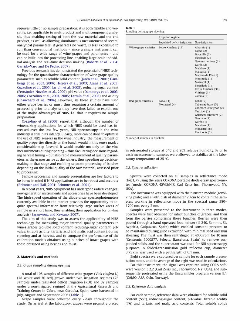
Table 1Sampling during grape ripening.
Irrigation regime
Regulated deficit irrigation Non-irrigation
White grape varieties Pedro Ximénez (19) Albariño (1)Baladí (2)Doradilla (3)Parellada (2)Gewurztraminer (1)Lairén (2)Macabeo (1)Malvasía (1)Mantuo de Pila (1)Montepila (1)Moscatel (1)Parrellada (1)Pedro Ximénez (38)Vijiriega (1)Zalema (3)
Red grape varieties Bobal (3)Monastrel (4)
Bobal (5)Cabernet Franc (3)Cabernet Sauvignon (2)Cencibel (1)Garnacha tintorera (2)Graciano (2)Lairén (1)Macabeo (1)Monastrel (5)Pinot noir (1)
Number of samples in brackets.
V. González-Caballero et al. / Journal of Food Engineering 101 (2010) 158–165 159
requires little or no sample preparation; it is both flexible and ver-satile, i.e., applicable to multiproduct and multicomponent analy-sis, thus enabling testing of both the raw material and the endproduct, as well as allowing simultaneous measurement of severalanalytical parameters; it generates no waste, is less expensive torun than conventional methods – since a single instrument canbe used for a wide range of wine grapes and parameters – andcan be built into the processing line, enabling large-scale individ-ual analysis and real-time decision making (Roberts et al., 2004;Garrido-Varo and De Pedro, 2007).
Previous research has demonstrated the potential of NIRS tech-nology for the quantitative characterization of wine grape qualityparameters such as soluble solid content (Jarén et al., 2001; Dam-bergs et al., 2003, 2006; Herrera et al., 2003; Arana et al., 2005;Cozzolino et al., 2005; Larraín et al., 2008), reducing-sugar content(Fernández-Novales et al., 2009), pH-value (Dambergs et al., 2003,2006; Cozzolino et al., 2004, 2005; Larraín et al., 2008) and acidity(Chauchard et al., 2004). However, all these studies have usedeither grape berries or must, thus requiring a certain amount ofprocessing prior to analysis; they have thus failed to exploit oneof the major advantages of NIRS, i.e. that it requires no samplepreparation.
Cozzolino et al. (2006) report that, although the number ofwinemaking applications for which NIRS could be used has in-creased over the last few years, NIR spectroscopy in the wineindustry is still in its infancy. Clearly, more can be done to optimisethe use of NIRS sensors in the wine industry; the measurement ofquality properties directly on the bunch would in this sense mark aconsiderable step forward. It would enable not only on-the-vinemeasurements during ripening – thus facilitating decisions regard-ing harvest timing – but also rapid measurement of quality param-eters as the grapes arrive at the winery, thus speeding up decision-making at that stage and enabling separate processing of batchesdepending on the initial quality of the raw material, assessed priorto processing.
Sample processing and sample presentation are key factors tobe borne in mind if NIRS applications are to be robust and accurate(Brimmer and Hall, 2001; Brimmer et al., 2001).
In recent years, NIRS equipment has undergone radical changes;new-generation instruments and accessories have been developed.The high-speed operation of the diode-array spectrophotometerscurrently available in the market provides the opportunity to ac-quire spectral information from relatively large surface areas ofsample in a short time, thus enabling their application for on-lineanalysis (Saranwong and Kawano, 2007).
The aim of this study was to assess the applicability of NIRStechnology for measuring major internal quality parameters inwines grapes (soluble solid content, reducing-sugar content, pH-value, titrable acidity, tartaric acid and malic acid content), duringripening and at harvest, and to compare the performance of thecalibration models obtained using bunches of intact grapes withthose obtained using berries and must.
2. Materials and methods
2.1. Grape sampling during ripening
A total of 108 samples of different wine grapes (Vitis vinifera L.)(78 white and 30 red) grown under two irrigation regimes (26samples under regulated deficit irrigation (RDI) and 82 samplesunder a non-irrigated regime) at the Agricultural Research andTraining Center in Cabra, near Cordoba, Spain, were harvested inJuly, August and September 2006 (Table 1).
Grape samples were collected every 7 days throughout thestudy. On arrival at the laboratory, grapes were promptly placed
in refrigerated storage at 0 �C and 95% relative humidity. Prior toeach measurement, samples were allowed to stabilize at the labo-ratory temperature of 25 �C.
2.2. Spectra collection
Spectra were collected on all samples in reflectance mode(log 1/R) using the Zeiss CORONA portable diode-array spectrome-ter (model CORONA 45VIS/NIR, Carl Zeiss Inc., Thornwood, NY,USA).
The instrument was equipped with the turnstep module (revol-ving plate) and a Petri dish of diameter 20 cm to contain the sam-ples, working in reflectance mode in the spectral range 380–1700 nm, every 2 nm.
Samples were presented to the instrument in three modes.Spectra were first obtained for intact bunches of grapes, and thenfrom the berries comprising these bunches. Berries were thenpassed through a hand-operated food mincer (LI 240, Sammic, SL,Azpeitia, Guipúzcoa, Spain) which enabled constant pressure tobe maintained during juice extraction with minimal seed and skinshearing. The must was then centrifuged at 4000 rpm for 10 min(Centronic 7000577, Selecta, Barcelona, Spain) to remove sus-pended solids, and the supernatant was used for NIR spectroscopypurposes. A folded-transmission gold reflector cup, diameter3.75 cm, was used with a pathlength of 0.1 mm.
Eight spectra were captured per sample for each sample presen-tation mode, and the average of the eight was used in calculations.
For this instrument, the signal was captured using CORA soft-ware version 3.2.2 (Carl Zeiss Inc., Thornwood, NY, USA), and sub-sequently pretreated using the Unscrambler program version 9.1(CAMO, ASA, Oslo, Norway).
2.3. Reference data analysis
For each sample, reference data were obtained for soluble solidcontent (SSC), reducing-sugar content, pH-value, titrable acidity(TA) and tartaric and malic acid contents. Total soluble solids

160 V. González-Caballero et al. / Journal of Food Engineering 101 (2010) 158–165
(�Brix) were measured using an Abbé-type refractometer (model B,Zeiss, Oberkochen, Württemberg, Germany). Reducing-sugar con-tent was measured by titration using an automatic titrator (CrisonMicro TT 2050, Crison, Alella, Barcelona, Spain), using a modifica-tion of the Rebelein method (Rebelein, 1971). Results were ex-pressed as g/l. Must pH-value and titrable acidity were measuredusing an automatic titrator (Crison Micro TT 2050, Crison, Alella,Barcelona, Spain); titrable acidity was measured by titration with0.1 NaOH to an end point of pH-value 7.0. Results were expressedas g/l tartaric acid (OJEU, 2005). Tartaric acid was measured with aspectrophotometer (HP 8452, Hewlett–Packard, Bristol, UK) as pre-viously described by Rebelein (1969), and expressed as g/l tartaricacid. Malic acid was measured using a portable RQflex reflectome-ter (model 16970, Merck Co., Darmstadt, Germany) using the en-zyme method (M.A.P.A., 1993). Results were expressed as g/lmalic acid.
2.4. Calibration and validation sets
Calibration models were initially developed using all the sam-ples available (n = 108), in order to establish the potentiality ofbunch presentation and to compare with those obtained for thetraditional models (berries and must) (Table 2).
Following, the best prediction models obtained for bunch pre-sentation were externally validated. For that, the initial sample setwas divided in two sets: 88 samples were used for calibration(80%), and 48 for external validation (20%) (Table 3). Samples to beused for both sets were selected solely on the basis of spectral data,following the method proposed by Shenk and Westerhaus (1991)using the CENTER algorithm included in the WinISI II software pack-age version 1.50 (Infrasoft International, Port Matilda, PA, USA).
2.5. Chemometric data treatment
The WinISI II software package version 1.50 was used for thechemometric treatment of data (ISI, 2000).
Quantitative calibrations were developed for predicting solublesolid content, reducing-sugar content, pH-value, titrable acidity,tartaric acid and malic acid contents in bunches and comparedwith those obtained for berries and must.
Prediction equations were obtained using the Modified PartialLeast Squares (MPLS) regression method (Shenk and Westerhaus,1995a). Partial least squares (PLS) regression is similar to principalcomponent regression (PCR), but uses both reference data (chemi-cal, physical, etc.) and spectral information to identify the factorsuseful for fitting (Martens and Naes, 1989). MPLS is often more sta-ble and accurate than the standard PLS algorithm. In MPLS, the NIRresiduals at each wavelength, obtained after each factor is calcu-lated, are standardized (divided by the standard deviations of theresiduals at a wavelength) before calculating the next factor. Whendeveloping MPLS equations, cross-validation is recommended toselect the optimal number of factors and to avoid overfitting(Shenk and Westerhaus, 1995a). For cross-validation, the calibra-tion set was partitioned into four groups; each group was then val-idated using a calibration developed on the other samples; finally,validation errors were combined to obtain a standard error ofcross-validation (SECV).
All multivariate regression equations were obtained using theStandard Normal Variate and Detrending methods for scatter cor-rection (Barnes et al., 1989). Moreover, four derivate mathematicaltreatments were tested in the development of NIRS calibrations: 1,5, 5, 1; 2, 5, 5, 1; 1, 10, 5, 1 and 2, 10, 5, 1 (Shenk and Westerhaus,1995b).
The following spectral regions were tested for calibration pur-poses on the instrument: 380–1650 nm (the higher spectral rangewith useful information covering the VIS + NIR regions); 780–
1650 nm (higher spectral range covering the NIR region andincluding the very near-infrared region) and 1100–1650 nm(including only the strict near-infrared region). In order to elimi-nate noise at the end of the spectral range, the region between1650 and 1700 nm was discarded.
The statistics used to select the best equations were: standarderror of calibration (SEC), coefficient of determination of calibra-tion (R2), standard error of cross-validation (SECV), coefficient ofdetermination for cross-validation (r2), RPD or ratio of the standarddeviation of the original data (SD) to SECV, and the coefficient ofvariation (CV) or ratio between the SECV and the mean value ofthe reference data of the studied parameter for the training set.This statistic enables SECV to be standardized, facilitating the com-parison of the results obtained with sets of different means (Wil-liams, 2001).
The best-fitting equations obtained for the calibration set(n = 88), as selected by statistical criteria, were subsequently eval-uated by external validation, a procedure determining the predic-tive ability of an equation based on a sample set which has notbeen used in the calibration procedures. This statistical process isbased on the determination of a known significant error, termed‘‘bias”, and an unexplained significant error, termed SEP(c) (stan-dard error of performance, bias-corrected) (Windham et al., 1989).
Generally, for calibration groups comprising more than 100, andvalidation groups containing 9 or more samples, the following con-trol limits are assumed (Shenk et al., 1989; Shenk and Westerhaus,1996):
Limit Control SEP(c) = 1.30 � SEC (standard error of calibration).Limit Control bias = ±0.60 � SEC (standard error of calibration).
3. Results and discussion
3.1. Spectral features
Typical log(1/R) spectra for bunches and berries, together withthe most relevant absorption bands, are shown in Fig. 1. In thespectral region studied, spectra for bunches and berries displayedvery similar behavior. The effect of derivatives was most apparentwith the first derivative of a spectrum, which was able to separateoverlapping absorption bands, displaying more clearly certaincharacteristic absorbance peaks.
For bunches and berry samples, three peaks were identified inthe visible region of the spectrum, at 430, 494 and 676 nm, respec-tively; these are indicative of the presence of red pigments (carote-noids and anthocyanins) and of abundant chlorophyll a and b(Strayer, 1995; McGlone and Kawano, 1998; McGlone et al., 2002).
In the near-infrared region, the spectrum was dominated by asugar-related absorption band at around 1200 nm region (Wil-liams, 2001). Water-related absorption bands were also found ataround 950 and 1460 nm, which are related to the third overtoneof O–H, as is usually the case for fruits and vegetables, particularlygrapes which 70–80% water (Murray, 1987; McGlone and Kawano,1998; Williams, 2001).
3.2. Population characterization
Statistical analysis of calibration sample sets, i.e., data ranges,means and standard deviations (SD) and coefficients of variation(CV) are shown in Tables 2 and 3. Samples were collected overthe critical months to check for SSC (15.3–58.6 �Brix), for titrableacidity (0.2–11.7 g/l tartaric acid) and for tartaric acid (4.9–15.5 g/l tartaric acid) variations in the berry.
A key feature of the sample set is that it contained data fromwine grapes sampled at different stages of ripening; this would ac-count for the high coefficient of variation (CV) values recorded,

0.6
0.7
0.8
0.9
1
1.1
1.2
1.3
1.4
1.5
380 580 780 980 1180 1380 1580
Log
(1/R
)
Wavelength (nm)
BunchesBerries
676
494
986
1204
1460
430
-0.6
-0.4
-0.2
0
0.2
0.4
0.6
0.8
380 580 780 980 1180 1380 1580
D1
(Log
1/R
)
Wavelength (nm)
BunchesBerries
506
654
682
946
972
1018
1134
1226
1322
1488 1636
Fig. 1. Typical log(1/R) and D1 log(1/T) spectra for grape bunches and berries.
Table 2Statistical analysis of calibration sample sets, i.e., data ranges, means and standarddeviations (SD) and coefficients of variation (CV).
Parameter Item
Number Range Mean Standarddeviation
CV (%)
Soluble solidcontent (�Brix)
108 15.30–58.60
23.86 7.46 31.29
Reducing-sugarcontent (g/l)
108 126.50–586.40
238.69 75.11 31.47
pH-value 108 2.90–4.60
3.54 0.34 9.51
Titrable acidity (g/ltartaric acid)
108 0.20–11.70
4.75 1.56 32.94
Tartaric acid (g/ltartaric acid)
108 4.90–15.50
7.53 1.65 21.97
Malic acid (g/l malicacid)
108 0.10–7.20
0.84 0.95 112.53
Table 3Statistical analysis of the calibration and prediction sample sets, i.e., data range, meanand standard deviation (SD) and coefficient of variation (CV).
Parameter Item Calibration set(n = 88)
Validation set(n = 20)
Soluble solid content(�Brix)
Range 15.30–58.60 16.40–25.90Mean 24.66 20.53SD 8.00 2.33CV (%) 32.44 11.34
Reducing-sugar content(g/l)
Range 126.50–586.40 156.1–269.0Mean 246.80 203.31SD 79.58 27.7CV (%) 32.24 13.62
pH-value Range 2.90–4.60 2.90–3.80Mean 3.58 3.39SD 0.34 0.27CV (%) 9.45 7.96
Titrable acidity (g/ltartaric acid)
Range 0.20–11.70 3.50–9.70Mean 4.55 5.45SD 1.43 1.84CV (%) 31.53 33.76
Tartaric acid (g/l tartaricacid)
Range 4.90–15.50 6.00–12.20Mean 7.39 8.00SD 1.62 1.76CV (%) 21.91 22.00
Malic acid (g/l malic acid) Range 0.10–7.20 0.30–2.00Mean 0.85 0.78SD 1.04 0.44CV (%) 122.35 56.41
V. González-Caballero et al. / Journal of Food Engineering 101 (2010) 158–165 161
particularly for soluble solid content, reducing-sugar content, titra-ble acidity, tartaric acid and malic acid contents.
The broad range of values recorded for SSC (15.30–58.60 �Brix)was due to the fact that sampling was carried out throughout rip-ening, which is characterized, amongst other things, by accumula-tion of sugars in the grape (López et al., 2007). The highest valueswere found for over-ripe samples which were over-ripe and wereto be used for drying into raisins.
Variations in acidity-related parameters (titrable acidity, tar-taric and malic acid content) were due to a decline in grape acidityduring ripening, as a result of the consumption of these two pre-dominant acids during fruit respiration (Peynaud, 1996).
It should be stressed that tartaric acid content varied withinnarrow limits. Absolute content underwent virtually no change
during ripening, although concentrations declined as the grapegained weight. At the end of ripening, tartaric acid content maydiminish due to combustion and precipitation as potassium bitar-trate (Alexiandre and Álvarez, 2003).
By contrast, malic acid levels fell steadily throughout ripening,displaying a more marked decline when external temperatureswere higher (López et al., 2009). The lowest values for malic acidwere therefore recorded at the end of ripening, and the highest val-ues were found in the initial samples.
3.3. Calibration development
3.3.1. Sweetness-related parametersThe best calibration models obtained using the global set
(n = 108) for the prediction of SSC and reducing-sugar contentaccording to the spectral range and derivate treatment used, forbunches, berries and musts are shown in Table 4.
The equation displaying the greatest predictive capacity for SSCin bunches was that obtained over the broadest spectral range, i.e.,380–1650 nm, with statistical values of r2 = 0.89, SECV = 1.41 �Brixand RPD = 2.92. The predictive capacity of this equation was higherto that of the equation obtained with grape must (RPD = 2.64) andlower than that recorded using berries (RPD = 3.34). Results forberries were similar to findings reported by Larraín et al. (2008):r2 = 0.91, RMSEP = 1.24 �Brix and RPD = 3.40.
It should be stressed that although the statistics obtained using‘‘bunch analysis” were similar to those recorded using traditionalNIRS presentation modes (berries and must), the overall equationpresented a coefficient of determination (0.89) that enabled sam-ples to be classed with total accuracy due to the excellence predic-tive capacity of the model (Williams, 2001). This was achievedusing a rapid, non-destructive sensor, and with no need for sampleprocessing, thus providing the wine industry with an instant re-sponse and enabling grape harvesting to be started at the optimumtime, as well as allowing musts to be processed selectively depend-ing on raw material characteristics assessed without priorprocessing.

Table 4Calibration statistics for the equations obtained for predicting soluble solid content (SSC) and reducing-sugar content for the different sample presentations and spectral rangesstudied (calibration set, n = 108 samples).
Parameter Samplepresentation
Spectral range (nm) Mathematictreatment
Meana SDb SECc R2d SECVe r2f RPDg CV (%)h
SSC (�Brix) Bunch 380–1650 2, 10, 5, 1 22.42 4.12 1.03 0.94 1.41 0.89 2.92 6.29i
780–1650 2, 5, 5, 1 22.51 3.83 1.03 0.93 1.52 0.85 2.53 6.731100–1650 1, 10, 5, 1 23.44 7.27 1.90 0.93 2.29 0.90 3.18 9.75
Berry 1100–1650 1, 10, 5, 1 22.66 4.77 1.07 0.95 1.43 0.91 3.34 6.31j
Must 380–1650 1, 5, 5, 1 22.81 4.81 1.26 0.93 1.82 0.86 2.64 7.98i
Reducing-sugar content (g/l)
Bunch 380–1650 2, 5, 5, 1 227.09 50.90 14.52 0.92 19.97 0.85 2.55 8.79780–1650 1, 5, 5, 1 223.41 47.38 11.76 0.94 17.13 0.87 2.77 7.67i
1100–1650 1, 10, 5, 1 222.69 47.62 11.38 0.94 18.95 0.84 2.51 8.51Berry 1100–1650 2, 10, 5, 1 221.69 51.17 9.16 0.97 13.10 0.93 3.91 5.91j
Must 780–1650 2, 5, 5, 1 227.73 50.93 21.20 0.83 26.39 0.73 1.93 11.59i
a Mean of the calibration set.b Standard deviation.c Standard error of calibration.d Coefficient of determination of calibration.e Standard error of cross-validation.f Coefficient of determination of cross-validation.g Ratio SD/SECV.h Coefficient of variation.i Best equation.j The best of the best equations for each sample presentation.
162 V. González-Caballero et al. / Journal of Food Engineering 101 (2010) 158–165
For reducing-sugar content, the equation displaying the great-est predictive capacity in bunches was obtained over the range780–1650 mm, yielding statistical values of r2 = 0.87, SECV =17.13 g/l and RPD = 2.77, i.e., lower to those obtained for berrysamples (r2 = 0.93, SECV = 13.10 g/l and RPD = 3.91) and higher tothose obtained for must samples (r2 = 0.73, SECV = 26.39 g/l andRPD = 1.93).
No published studies address the direct measurement of reduc-ing-sugar content in grapes. Fernández-Novales et al. (2009) re-ported a greater predictive capacity in musts (r2 = 0.98,SECV = 13.62 g/l and RPD = 6.57), although their results are notwholly comparable, since they used a set comprising not only re-cently-pressed grape musts – as was the case here – but also fer-menting musts and finished wines, and thus were able to use amore varied calibration set.
3.3.2. Acidity-related parametersFor pH-value, the best statistics (r2 = 0.69, SECV = 0.19 and
RPD = 1.81) for bunch analysis were obtained with the second der-ivate treatment (math treatment 2, 10, 5, 1) in the spectral range380–1650 nm (Table 5). The value obtained for r2 (0.69) would,according to the guidelines indicated by Williams (2001), enablethe classification of musts obtained from these grapes into threecategories (high, medium and low pH-value), thus allowing muststo be adjusted prior to fermentation.
Interestingly, bunch analysis yielded better results than theother presentation modes for pH-value (RPD = 1.81), followed byberry analysis (RPD = 1.66), and finally must analysis (RPD = 1.43).
The results obtained using bunch analysis, though more com-plex and less uniform, matched those reported by Cozzolino et al.(2004) (r2 = 0.72, RMSECV = 0.068 and RPD = 1.4) in the spectralrange 700–1100 nm, and by Larraín et al. (2008) (r2 = 0.74,RMSEP = 0.15 and RPD = 2.2) working in the spectral range 640–1300 nm, in both cases with berries.
This study also measured other acidity-related parameters:titrable acidity, tartaric acid and malic acid content. The resultsare shown in Table 5. Measurement of acidity-related parametersin intact fruit is notoriously difficult (Flores et al., 2009); nonethe-less, the models developed for these three parameters suggestedthat NIRS technology may be used for screening purposes, to dis-tinguish between low and high acidity, as indicated by the values
obtained for the determination coefficient (r2 = 0.45 for titrableacidity; r2 = 0.49 for tartaric and malic acids) (Williams, 2001). Itis also important to note that the best equations for titrable acidity(r2 = 0.45 and SECV = 1.16 g/l) and tartaric acid content (r2 = 0.49and SECV = 1.20 g/l) were obtained using bunch analysis ratherthan the other presentation modes. Although better results wereobtained for malic acid content using berry analysis (r2 = 0.49and SECV = 0.68 g/l), the statistics obtained for bunch analysis indi-cated a similar predictive capacity (r2 = 0.41 and SECV = 0.74 g/l).Other authors measured total acidity (as the sum of tartaric andmalic acid contents) in red grape berries using a non-linear ap-proach and obtained higher predictive ability (r2 = 0.77 andSECV = 1.30 g/l) (Chauchard et al., 2004).
3.4. External validation
The aim was, in the first instance, to validate the best calibra-tion models using a sample set not included in the calibration,but similar to the calibration set. Validations of the best calibrationmodels obtained were performed using sets comprising 20 sam-ples (Table 3). Although several authors have reported that theSECV gives a realistic estimate of the error prediction of samplesnot included in the calibration (Meuret et al., 1993; Shenk andWesterhaus, 1996; Martens and Dardenne, 1998), this step is rec-ommended to obtain an independent measurement of the equa-tion’s accuracy, expressed as SEP, i.e., standard error ofperformance (Windham et al., 1989).
Only the calibrations that showed a predictive ability that couldbe considered as good were externally validated, i.e., those calibra-tions developed for the prediction of SSC, reducing sugars and pH(Table 6). For the rest of parameters related to acidity and due tothe lower values of the statistics obtained, it was not consideredappropriate at their development status, their validation.
On examining Table 6, it can be observed that the values ob-tained for the statistics SECV and SEP are very similar for the threeparameters studied, which confirms that it is correct to use theSECV as an estimator of the SEP. This aspect is especially importantwhen it is a case of obtaining calibration equations from groupswith a reduced number of samples, which it does apply to the pres-ent case, as small number of samples are involved in the calibra-tion and validation of equations. Moreover, using the monitoring

Table 5Calibration statistics for the equations obtained for predicting pH-value, titrable acidity, tartaric acid and malic acid contents for the different sample presentations and spectralranges studied (calibration set n = 108 samples).
Parameter Samplepresentation
Spectral range(nm)
Mathematictreatment
Meana SDb SECc R2d SECVe r2f RPDg CV (%)h
pH-value Bunch 380–1650 2, 10, 5, 1 3.54 0.34 0.15 0.78 0.19 0.69 1.81 5.26i
780–1650 2, 10, 5, 1 3.54 0.34 0.17 0.75 0.19 0.68 1.77 5.381100–1650 1, 10, 5, 1 3.54 0.34 0.19 0.66 0.21 0.63 1.63 5.81
Berry 380–1650 1, 5, 5, 1 3.54 0.34 0.19 0.68 0.20 0.64 1.66 5.75j
Must 780–1650 1, 10, 5, 1 3.54 0.34 0.22 0.57 0.24 0.49 1.43 6.66j
Titrable acidity (g/l tartaricacid)
Bunch 380–1650 1, 5, 5, 1 4.75 1.56 0.96 0.62 1.16 0.45 1.35 24.63i
780–1650 1, 10, 5, 1 4.75 1.56 1.05 0.54 1.21 0.40 1.29 25.651100–1650 1, 10, 5, 1 4.75 1.56 1.12 0.48 1.28 0.32 1.35 27.21
Berry 380–1650 1, 5, 5, 1 4.75 1.56 1.18 0.43 1.29 0.33 1.21 27.16j
Must 780–1650 1, 5, 5, 1 4.75 1.56 1.22 0.20 1.26 0.18 1.24 26.81j
Tartaric acid (g/l tartaric acid) Bunch 380–1650 2, 10, 5, 1 7.53 1.65 0.97 0.66 1.20 0.49 1.38 16.02i
780–1650 2, 10, 5, 1 7.53 1.65 1.04 0.60 1.22 0.47 1.36 16.261100–1650 1, 5, 5, 1 7.53 1.65 1.11 0.55 1.31 0.39 1.26 17.52
Berry 380–1650 2, 10, 5, 1 7.53 1.65 1.02 0.62 1.34 0.34 1.23 17.85j
Must 1100–1650 2, 10, 5, 1 7.53 1.65 1.38 0.02 1.389 0.01 1.19 18.83j
Malic acid (g/l malic acid) Bunch 380–1650 2, 5, 5, 1 0.84 0.95 0.51 0.71 0.74 0.41 1.28 88.42j
780–1650 2, 5, 5, 1 0.84 0.95 0.65 0.53 0.80 0.31 1.19 95.451100–1650 2, 5, 5, 1 0.84 0.95 0.72 0.43 0.85 0.21 1.11 101.92
Berry 380–1650 2, 5, 5, 1 0.84 0.95 0.44 0.79 0.68 0.49 1.40 80.18i
Must 1100–1650 2, 5, 5, 1 0.84 0.95 0.46 0.77 0.72 0.46 1.32 80.17j
a Mean of the calibration set.b Standard deviation.c Standard error of calibration.d Coefficient of determination of calibration.e Standard error of cross-validation.f Coefficient of determination of cross-validation.g Ratio SD/SECV.h Coefficient of variation.i The best of the best equations for each sample presentation.j Best equation.
Table 6Main calibration and validation statistics and control limits for predicting soluble solid content (SSC), reducing-sugar content and pH.
Parameter Sample presentation Calibration Prediction Control limits
R2a SECb r2c SECVd r2e SEPf SEP(c)g Bias SEP(c) Bias
SSC (�Brix) Bunch 0.96 1.04 0.91 1.53 0.57 1.63 1.69 0.05 1.35 ±0.62Reducing-sugar content (g/l) Bunch 0.93 12.96 0.87 17.40 0.61 17.94 17.69 �5.36 16.85 ±7.78pH-value Bunch 0.90 0.10 0.79 0.15 0.51 0.19 0.19 �0.01 0.13 ±0.06
a Coefficient of determination of calibration.b Standard error of calibration.c Coefficient of determination of cross-validation.d Standard error of cross-validation.e Coefficient of determination of prediction.f Standard error of prediction.g Standard error of prediction bias-corrected.
V. González-Caballero et al. / Journal of Food Engineering 101 (2010) 158–165 163
procedure proposed by Shenk et al. (1989), for the three qualityparameters studied, it is important to emphasize that the SEP(c)
values are close to the confidence limits and the bias are belowthe confidence limits, showing that the three NIRS equations canbe considered as a first trial to develop accurate predictions usingthe bunch as sample presentation mode.
3.5. Effective wavelengths for predicting soluble solid content,reducing-sugar content and pH-value
The loading plots corresponding to the best models obtained forpredicting soluble solid content, reducing-sugar content and pH-value are shown in Fig. 2. These plots show the areas across thespectral range where variance has influenced computing of themodel to a greater or lesser degree, and the direction (positive ornegative).
For the prediction of soluble solid content in grapes, representa-tion of the four latent variables (LV) used in constructing the cali-bration equation shows that the areas of the spectrum exertinggreatest weight on model fitting were 728, 948, 976, 1138 and1384 nm, related to the absorption of glucids and water (Fig. 2).The absorption around 948 nm was also relevant for reducing-su-gar content (Fernández-Novales et al., 2008), while 976 nm was re-lated to the second overtone of O–H in sugars (Osborne et al.,1993).
For the prediction of reducing-sugar content, the wavelengthsexerting greatest weight were 720, 948, 982, 1034, 1138, 1284and 1384 nm, also associated with glucid and water absorption;their influence was either positive or negative, depending on thelatent variable in question. The wavelength at around 950 nmwas relevant for measuring reducing-sugar content, as reportedby Fernández-Novales et al. (2008, 2009). Absorption at around960 nm was also related to the third overtone of O–H of water

-0.6
-0.4
-0.2
0
0.2
0.4
0.6
0.8
1
1.2
1.4
X-Lo
adin
g w
eigh
ts
Wavelength (nm)
Soluble solids content LV 1 (41%) LV 2 (28%)
LV 3 (20%) LV 4 (4%)
-0.6
-0.4
-0.2
0
0.2
0.4
0.6
0.8
1
1.2
X-Lo
adin
g w
eigh
ts
Wavelength (nm)
Reducing sugars content LV 1 (41%) LV 2 (28%)
LV 3 (20%) LV 4 (4%)
-2
-1
0
1
2
3
4
5
700 800 900 1000 1100 1200 1300 1400 1500 1600
700 800 900 1000 1100 1200 1300 1400 1500 1600
700 800 900 1000 1100 1200 1300 1400 1500 1600
X-Lo
adin
g w
eigh
ts
Wavelength (nm)
pH-value LV 1 (50%) LV 2 (38%)
LV 3 (6%) LV 4 (3%)
Fig. 2. X-Loading weights for soluble solid content and reducing-sugar content inberries and for pH-value in bunches.
164 V. González-Caballero et al. / Journal of Food Engineering 101 (2010) 158–165
(Williams, 2001), and the absorption at around 975 nm with solu-ble solid content (Shao and He, 2007).
For the prediction of pH-value, the wavelengths exerting great-est weight were 768 nm, associated with C–H stretch fourth over-tones, 986 nm associated to the second overtone of O–H in sugars,1152 nm associated with C–H second overtones, and 1330, 1376and 1418 nm associated with water absorption (Osborne et al.,1993).
4. Conclusions
These results suggest that NIRS is a very promising and usefulsensor for the non-destructive quantification of chemical changestaking place during on-vine ripening, and for deciding on the opti-mum time for harvesting.
It must be highlighted that the results obtained here with theanalysis of grapes in bunch form, requiring no previous samplepreparation, should be considered a first step in the tuning of NIRS
technology for on-site and on-line control purposes, since it is theform in which the grape grows, and in which it arrives at the win-ery. Application of NIRS will enable increased sampling of eachbatch produced, thus ensuring a more precise and accurate guaran-tee of specific quality. As a result, rapid decisions can be takenregarding the optimum harvesting time, and fruit arriving at thewinery can be swiftly streamed, allowing batches to be processedseparately depending on initial grape quality.
References
Alexiandre, J.L., Álvarez, I., 2003. Tecnología Enológica. Síntesis, Madrid, España.Arana, I., Jarén, C., Arazuri, S., 2005. Maturity, variety and origin determination in
white grapes (Vitis vinifera L.) using NIRS. Journal of Near Infrared Spectroscopy13, 349–357.
Barnes, R.J., Dhanoa, M.S., Lister, S.J., 1989. Standard normal variate transformationand de-trending of near infrared diffuse reflectance spectra. AppliedSpectroscopy 43, 772–777.
Brimmer, P.J., Hall, J.W., 2001. Method development and implementation of Near-Infrared Spectroscopy in industrial manufacturing support laboratories. In:Williams, P., Norris, K. (Eds.), Near-Infrared Technology in the Agricultural andFood Industries, second ed. American Association of Cereal Chemist, Minnesota,USA, pp. 187–198.
Brimmer, P.J., DeThomas, F.A., Hall, J.W., 2001. Method 370 development andimplementation of Near-Infrared Spectroscopy in industrial manufacturingprocesses. In: Williams, P., Norris, K. (Eds.), Near-Infrared Technology in theAgricultural and Food Industries, second ed. American Association of CerealChemist, Minnesota, USA, pp. 199–214.
Chauchard, F., Codgill, R., Roussel, S., Roger, J.M., Bellon-Meurel, V., 2004.Application of LS-SVM to non-linear phenomena in NIR spectroscopy:development of a robust and portable sensor for acidity prediction in grapes.Chemometrics and Intelligent Laboratory Systems 71, 141–150.
Cozzolino, D., Esler, M.B., Dambergs, R.G., Cynkar, W.U., Boehm, D.R., Francis, I.L.,Gishen, M., 2004. Prediction of color and pH in grapes using a diode arrayspectrophotometer (400–1100 nm). Journal of Near Infrared Spectroscopy 12,105–111.
Cozzolino, D., Cynkar, W.U., Dambergs, R.G., Janik, L., Gishen, M., 2005. Effect of bothhomogenisation and storage on the spectra of red grapes and on themeasurement of total anthocyanins, total soluble solids and pH by visual nearinfrared spectroscopy. Journal of Near Infrared Spectroscopy 13, 213–223.
Cozzolino, D., Dambergs, R.G., Janik, L., Cynkar, W.U., Gishen, M., 2006. Analysis ofgrapes and wine by near infrared spectroscopy. Journal of Near InfraredSpectroscopy 14, 279–289.
Dambergs, R.G., Cozzolino, D., Cynkar, W.U., Kambouris, A., Francis, I.L., Høj, P.B.,Gishen, M., 2003. The use of near infrared spectroscopy for grape qualitymeasurement. Australian Grapegrower and Winemaker 476, 69–76.
Dambergs, R.G., Cozzolino, D., Cynkar, W.U., Janik, L., Gishen, M., 2006. Thedetermination of red grape quality parameters using the LOCAL algorithm.Journal of Near Infrared Spectroscopy 14, 71–79.
Fernández-Novales, J., López, M.I., Sánchez, M.T., García, J.A., Morales, J.A., 2008. Afeasibility study on the use of a miniature fiber optic NIR spectrometer for theprediction of volumic mass and reducing sugar content in white winefermentations. Journal of Food Engineering 89, 325–329.
Fernández-Novales, J., López, M.I., Sánchez, M.T., Morales, J., González-Caballero, V.,2009. Shortwave-near infrared spectroscopy for determination of reducingsugar content during grape ripening, winemaking and aging of white and redwines. Food Research International 42, 285–291.
Flores, K., Sánchez, M.T., Pérez-Marín, D.C., Guerrero, J.E., Garrido-Varo, A., 2009.Feasibility in NIRS instruments for predicting internal quality in intact tomato.Journal of Food Engineering 91, 311–318.
Garrido-Varo, A., De Pedro, E., 2007. The role of Near-Infrared Spectroscopy inverifying label information in agro-forestry. In: Burns, D.A., Ciurczak, E.W.(Eds.), Handbook of Near-Infrared Spectroscopy Analysis, third ed., PracticalSpectroscopy Series, vol. 35 CRC Press, USA, pp. 387–398.
Gishen, M., Dambergs, R.G., Kambouris, A., Kwiatkowski, M., Cynkar, W.U., Høj, P.B.,2000. Application of near infrared spectroscopy for quality assessment ofgrapes, wine and spirits. In: Davies, A.M.C., Giangiacomo, R. (Eds.), Proceedingsof the Ninth International Conference on Near Infrared Spectroscopy. NIRPublications, Chichester, UK, pp. 917–920.
Gishen, M., Iland, P.G., Dambergs, R.G., Esler, M.B., Francis, I.L., Kambouris, A., 2002.Objective measures of grape and wine quality. In: Blair, R.J., Williams, P.J., Hoj,P.B. (Eds.), Proceedings of the 11th Australian Wine Industry TechnicalConference. The Australian Wine Research Institute, Urrbrae, SA, Australia, pp.188–194.
Herrera, J., Guesalaga, A., Agosin, E., 2003. Shortwave-near infrared spectroscopy fornon-destructive determination of maturity of wine grapes. MeasurementScience and Technology 14, 689–697.
ISI, 2000. The Complete Software Solution Using a Single Screen for RoutineAnalysis, Robust Calibrations and Networking. Manual, FOSS NIRSystems/TECATOR. Infrasoft International, LLC, Silver Spring, MD.
Jarén, C., Ortuño, J.C., Arazuri, S., Arana, J.I., Salvadores, M.C., 2001. Sugardetermination in grapes using NIR technology. International Journal ofInfrared and Millimeter Waves 22, 1521–1530.

V. González-Caballero et al. / Journal of Food Engineering 101 (2010) 158–165 165
Larraín, M., Guesalaga, A.R., Agosin, E., 2008. A multipurpose portable instrumentfor determining ripeness in wine grapes using NIR spectroscopy. IEEETransactions on Instrumentation and Measurement 57, 294–302.
López, M.I., Sánchez, M.T., Díaz, A., Ramírez, P., Morales, J., 2007. Influence of adeficit irrigation regime during ripening on berry composition in grapevines(Vitis vinifera L.) grown in semiarid areas. International Journal of Food Scienceand Nutrition 58, 491–507.
López, M.I., Sánchez, M.T., Ramírez, P., Morales, J., 2009. Effect of a deficit irrigationregime on the quality of wines made from white grapes (Vitis vinifera L.) grownin semiarid areas. Journal of Food Quality 32, 481–503.
M.A.P.A. (Spanish Ministry of Agriculture, Fisheries and Food), 1993. OfficialMethods for the Analysis of Wines. Secretaría General de Alimentación,vol. II. Dirección General de Política Alimentaria, Madrid, España. pp. 35–319.
Martens, H.A., Dardenne, P., 1998. Validation and verification of regression in smalldata sets. Chemometrics and Intelligent Laboratory Systems 44, 99–121.
Martens, H., Naes, T., 1989. Multivariate Calibration. John Wiley & Sons, Chichester,UK.
Martínez-Toda, F., 2007. Claves de la Viticultura de Calidad: Nuevas Técnicas deEstimación y Control de la Calidad de la Uva en el Viñedo. Mundi-Prensa LibrosS.A., Madrid, España.
McGlone, V.A., Kawano, S., 1998. Firmness, dry matter and soluble solidsassessment of postharvest kiwifruit by NIR spectroscopy. Postharvest Biologyand Technology 13, 131–141.
McGlone, V.A., Jordan, R.B., Martinsen, P.J., 2002. Vis/NIR estimation at harvest ofpre and post-storage quality indices for ‘‘Royal Gala” apple. Postharvest Biologyand Technology 25, 135–144.
Meuret, M., Dardenne, P., Biston, R., Poty, O., 1993. The use of NIR in predictingnutritive value of Mediterranean tree and shrub foliage. Journal of Near InfraredSpectroscopy 1, 45–54.
Murray, I., 1987. The NIR spectra of homologous series of organic compounds. In:Hollow, J., Kaffka, K.J., Gonczy, J.L. (Eds.), Near Infrared Diffuse Reflectance/Transmittance Spectroscopy. Proceedings of the International NIR/NITConference, Akademiai Kiado, Budapest, pp. 13–28.
Official Journal of the European Union (OJEU), 2005. Commission Regulation (EC)No. 1293/2005 of 5 August 2005 Amending Regulation (EEC) No. 2676/90determining Community Methods for the Analysis of Wines. Official Journal L205, 6 of August, pp. 12–15.
Osborne, B.G., Fearn, T., Hindle, P.H., 1993. Practical NIR spectroscopy withapplications. In: Osborne, B.G., Fearn, T., Hindle, P.H. (Eds.), Food andBeverage Analysis. Longman, Essex, UK, pp. 11–35.
Peynaud, E., 1996. Enología Práctica. Conocimientos y Elaboración del Vino. Mundi-Prensa Libros S.A., Madrid, España.
Rebelein, H., 1969. Dosage rapide de l’acide tartrique. Office International de laVigne et du Vin, Feuillet Vert. 431.
Rebelein, H., 1971. Correction de l’acidité des moûts et des vins. Bulletin de lOIV 480(44), 136–141.
Roberts, C.A., Stuth, J., Flinn, P., 2004. Analysis of forages and feedingstuffs. In:Roberts, C.A., Workman, J., Reeves, J.B., III (Eds.), Near-Infrared Spectroscopy inAgriculture. ASA, CSSA y SSSA Inc., Madison, WI, USA, pp. 231–267.
Saranwong, S., Kawano, S., 2007. Applications to agricultural and marine products:fruits and vegetables. In: Ozaki, Y., McClure, W.F., Christy, A.A. (Eds.), Near-Infrared Spectroscopy in Food Science and Technology. John Wiley & Sons Inc.,Hoboken, NJ, pp. 219–242.
Sas, A., 2008. The missing gap: measuring and paying for grape quality. In: Blair, R.,Williams, P., Pretorius, S. (Eds.), Proceedings of the 13th Australian WineIndustry Technical Conference. The Australian Wine Research Institute, Urrbrae,SA, Australia, pp. 52–55.
Shao, Y., He, Y., 2007. Nondestructive measurement of the internal quality ofbayberry juice using Vis/NIR spectroscopy. Journal of Food Engineering 79,1015–1019.
Shenk, J.S., Westerhaus, M.O., 1991. Population definition sample selection andcalibration procedures for near infrared spectra and modified partial leastsquares regression. Crop Science 31, 469–474.
Shenk, J.S., Westerhaus, M.O., 1995a. Analysis of Agricultural and Food Products byNear Infrared Reflectance Spectroscopy. NIRSystems, Silver Spring, MD.
Shenk, J.S., Westerhaus, M.O., 1995b. Routine Operation, Calibration, Developmentand Network System Management Manual. NIRSystem, Silver Spring, MD.
Shenk, J.S., Westerhaus, M.O., 1996. Calibration the ISI way. In: Davies, A.M.C.,Williams, P.C. (Eds.), Near Infrared Spectroscopy: The Future Waves. NIRPublications, Chichester, West Sussex, UK, pp. 198–202.
Shenk, J.S., Westerhaus, M.O., Abrams, S.M., 1989. Protocol for NIR calibrations:monitoring analysis results and recalibration. In: Martens, G.C., Shenk, J.S.,Barton, F.E., II (Eds.), Near Infrared Spectroscopy (NIRS): Analysis of ForageQuality, Agriculture Handbook, vol. 643. USDA-ARS, US Government PrintingOffice, Washington, DC, pp. 104–110.
Strayer, L., 1995. Biochemistry, fourth ed. W.H. Freeman and Company/WorthPublishers, New York, USA.
Williams, P.C., 2001. Implementation of near-infrared technology. In: Williams, P.C.,Norris, K.H. (Eds.), Near-Infrared Technology in the Agricultural and FoodIndustries. AACC Inc., St. Paul, Minnesota, pp. 145–169.
Windham, W.R., Mertens, D.R., Barton II, F.E., 1989. Protocol for NIRS calibration:sample selection and equation development and validation. In: Martens, G.C.,Shenk, J.S., Barton, F.E., II (Eds.), Near Infrared Spectroscopy (NIRS): Analysis ofForage Quality, Agriculture Handbook, vol. 643. USDA-ARS, US GovernmentPrinting Office, Washington, DC, pp. 96–103.

NIRS para la predicción de parámetros de calidad interna y momento óptimo de cosecha en uvas y control de calidad y trazabilidad en la industria vitivinícola
______________________________________________________________________
99
4.2. EVALUATION OF DIFFERENT REGRESSION STRATEGIES FOR
INTERNAL QUALITY CONTROL OF GRAPE BUNCHES DURING ON-VINE
RIPENING. SENSORS 11, 6109-6124 (2011)

100

Sensors 2011, 11, 6109-6124; doi:10.3390/s110606109
sensors ISSN 1424-8220
www.mdpi.com/journal/sensors
Article
Optimization of NIR Spectral Data Management for Quality
Control of Grape Bunches during On-Vine Ripening
Virginia González-Caballero 1, Dolores Pérez-Marín
2,*, María-Isabel López
1 and
María-Teresa Sánchez 3,*
1 Centro de Investigación y Formación Agraria de ‗‗Cabra-Priego‖, Instituto de Investigación y
Formación Agraria y Pesquera (IFAPA), Consejería de Agricultura y Pesca, Junta de Andalucía,
Cabra, Spain; E-Mails: [email protected] (V.G.-C.);
[email protected] (M.-I.L.) 2 Department of Animal Production, University of Cordoba, Campus Rabanales, 14071 Cordoba,
Spain 3
Department of Bromatology and Food Technology, University of Cordoba, Campus Rabanales,
14071 Cordoba, Spain
* Authors to whom correspondence should be addressed; E-Mails: [email protected] (D.P.-M.);
[email protected] (M.-T.S.); Tel.: +34-957-21-2576; Fax: +34-957-21-2000.
Received: 10 May 2011, in revised form: 30 May 2011 / Accepted: 31 May 2011 /
Published: 7 June 2011
Abstract: NIR spectroscopy was used as a non-destructive technique for the assessment of
chemical changes in the main internal quality properties of wine grapes (Vitis vinifera L.)
during on-vine ripening and at harvest. A total of 363 samples from 25 white and red grape
varieties were used to construct quality-prediction models based on reference data and on
NIR spectral data obtained using a commercially-available diode-array spectrophotometer
(380–1,700 nm). The feasibility of testing bunches of intact grapes was investigated and
compared with the more traditional must-based method. Two regression approaches
(MPLS and LOCAL algorithms) were tested for the quantification of changes in soluble
solid content (SSC), reducing sugar content, pH-value, titratable acidity, tartaric acid, malic
acid and potassium content. Cross-validation results indicated that NIRS technology
provided excellent precision for sugar-related parameters (r2 = 0.94 for SSC and reducing
sugar content) and good precision for acidity-related parameters (r2 ranging between 0.73
and 0.87) for the bunch-analysis mode assayed using MPLS regression. At validation level,
comparison of LOCAL and MPLS algorithms showed that the non-linear strategy
OPEN ACCESS

Sensors 2011, 11
6110
improved the predictive capacity of the models for all study parameters, with particularly
good results for acidity-related parameters and potassium content.
Keywords: NIR spectroscopy; quality parameters; on-vine; bunch analysis
1. Introduction
The achievement of high quality standards in modern wine production depends on harvesting grapes
at the optimum stage of ripeness [1]. By determining the right moment for harvesting, winemakers can
ensure the best possible wine for any given year or conditions. For this purpose, it is essential to
measure a number of grape quality parameters, including soluble solid content, reducing-sugar content,
titratable acidity, pH-value, tartaric acid and malic acid contents and sensory attributes [2].
Flanzy [3] has noted that grape organic-acid content determines wine acidity, and also governs the
stability, color and acceptability of the final product, since a wine with the right amount of acidity
lingers longer on the palate. At the same time, accurate grape-quality measurements enable wineries to
stream fruit for crushing and blending, thus maximizing the profitability of their production [4].
Existing analytical methods for the measurement of grape and wine composition do not meet the
requirements of modern wine production in a global market, where there is a clear need for fast,
accurate, simultaneous and non-destructive measurement of quality parameters both in the raw
material and in the finished product [5-7].
Conventional laboratory techniques for measuring different quality characteristics in grapes and
wines are tedious, time-consuming and technically demanding, and thus constitute a barrier to the
widespread uptake and use of quality descriptors by the grape and wine industry [8].
Because certain variables change in the course of ripening, there is an evident need for non-invasive,
objective methods of constantly monitoring the ripening process [9]. These methods can also be used
to separate grapes of different qualities at harvest, thus increasing the economic value of the harvest as
a whole through product differentiation [10].
The potential of NIRS technology as a non-destructive method for the quantitative characterization
of grape quality parameters, using either grape berries or must, has been amply demonstrated [6,10-15].
However, all these studies have required a certain amount of data processing prior to analysis. The
authors have thus failed to exploit one of the major advantages of NIRS: the fact that it requires no
sample preparation, and is therefore very fast.
Although González-Caballero [7] have addressed the use of NIR spectroscopy models for predicting
SSC, reducing sugar content, pH-value, titratable acidity, tartaric acid levels and malic acid content in
whole grapes using a spectral range of up to 1,700 nm, the authors stress that the results obtained when
analyzing grapes in bunch form should only be considered a first step in the fine-tuning of NIRS
technology for on-site control purposes, and that the expectations aroused by NIRS technology for
quality control during the ripening process in intact grapes need to be confirmed by increasing the
sample set, with a view to improving the specificity, accuracy and robustness of the calibrations
obtained.

Sensors 2011, 11
6111
In practice, however, when new sample groups are included in the calibration set, robustness tends
to be increased at the expense of accuracy [16]. One way of overcoming this problem is to develop
specific calibrations for small groups of similar samples within the product domain [17]. The method
used, known as local regression, combines the advantages of global calibrations obtained using a
sample set large enough to ensure coverage of extensive product variation with the accuracy provided
by specific calibrations [17].
Dambergs [12] reported improved accuracy in models to predict grape anthocyanin content and pH
when sample subsets were selected on the basis of vintage, grape variety and growing region, due to a
reduction of calibration non-linearity; in their view, the LOCAL algorithm appears to provide a
practical solution to developing robust models for the prediction of these parameters in grapes. They
note, however, that the models constructed using MPLS and LOCAL algorithms performed equally
well for measuring total soluble solid content.
The aim of this study was to develop accurate and robust NIRS models for measuring major internal
quality parameters in intact wine grapes (soluble solid content, reducing sugar content, pH-value,
titratable acidity, tartaric acid, malic acid, and potassium content) during ripening and at harvest,
regardless of growing season or variety, with a view to enabling growers to routinely use NIRS
technology under field conditions to predict more precisely the timing of their harvest operations, and
thus ensure the highest possible grape and wine quality.
2. Material and Methods
2.1. Grape Sampling During Ripening
The sample set for all the parameters tested, except for potassium content, comprised 363 samples
of 25 different white and red wine grape varieties (Vitis vinifera L.). Grape bunches sourced from
experimental vineyards at the Agricultural Research Training Centre at Cabra, near Cordoba (Spain),
were harvested in July, August and September in 2006, 2007 and 2008. Grape samples were collected
every seven days throughout the study. On arrival at the laboratory, grapes were promptly placed in
refrigerated storage at 0 °C and 95% relative humidity. All samples were allowed to stabilize at room
temperature (20 °C) prior to Vis–NIR spectral analysis.
2.2. Spectrum Collection
Spectra were collected using a Zeiss CORONA portable and non-contact diode-array spectrometer
(model CORONA 45VIS/NIR, Carl Zeiss, Inc., Thornwood, NY, USA) equipped with the turnstep
module (revolving plate) and a 20-cm-diameter Petri dish to hold the samples, working in reflectance
mode in the spectral range 380–1,700 nm, every 2 nm. The measurement distance from the source of
light to the sample was 13 mm.
Samples were presented to the instrument in two modes. Spectra were first obtained for intact
bunches of grapes. Berries were then passed through a hand-operated food mincer (LI 240, Sammic,
SL, Azpeitia, Guipúzcoa, Spain) which enabled constant pressure to be maintained during juice
extraction with minimal seed and skin shearing. The must was then centrifuged at 4,000 rpm for
10 min (Centronic 7000577, Selecta, Barcelona, Spain) to remove suspended solids, and the

Sensors 2011, 11
6112
supernatant was used for NIR spectroscopy purposes. A folded-transmission gold reflector cup,
diameter 3.75 cm, was used with a pathlength of 0.1 mm.
Eight spectra were captured per sample for each sample presentation mode, and the average of the
eight was used in calculations. The signal was captured using CORA software version 3.2.2 (Carl
Zeiss, Inc., Thornwood, NY, USA), and subsequently pretreated using the Unscrambler version 9.1
program (CAMO, ASA, Oslo, Norway).
2.3. Reference Data Analysis
For each sample, reference data were obtained for SSC, reducing sugar content, pH-value, titratable
acidity, tartaric acid, malic acid and potassium content. SSC (°Brix), reducing sugar content, must
pH-value, titratable acidity, and tartaric and malic acid contents were measured as indicated by
González-Caballero [7]. Potassium content was measured using a CORNING 410 flame photometer
(Ciba Corning Diagnostics Limited, Halstead, UK) as previously described by the Spanish Ministry of
Agriculture, Fisheries and Food [18]. Results were expressed as milligrams per liter.
2.4. Calibration and Validation Sets
The sample set, except for potassium cation, comprised all the available samples (363 samples;
25 varieties) picked during ripening: 108 samples collected in 2006, 120 samples in 2007, and 135
samples in 2008. After eliminating as outliers (n = 2 samples for 2006; n = 4 samples for 2007;
n = 13 samples for 2008) those grapes considered over-ripe and thus displaying high sugar content, the
initial sample set was divided in two subsets: 251 samples (73% of the total) were used to construct
calibration models (calibration set), and the remaining 93 samples (27%), all picked in 2008, were
used for external validation (validation set). It should be stressed that the calibration set contained all
available samples from 2006 (106 samples) and 2007 (116 samples), together with 29 samples from
2008. These sets were used to develop and subsequently validate models to predict SSC, reducing
sugar content, pH-value, titratable acidity, tartaric acid, and malic acid. The calibration and validation
sets used to predict potassium content contained only samples from 2008: 104 (80%) for calibration
and 44 (20%) for external validation. In all cases, samples were selected solely on the basis of spectral
data, following Shenk and Westerhaus [19], using the CENTER algorithm included in the WinISI II
software package version 1.50 (Infrasoft International, Port Matilda, PA, USA) prior to developing
NIRS calibrations, in order to determine the structure and spectral variability of the study population.
This algorithm was applied over the samples belonged to 2008 season.
2.5. Chemometric Data Treatment
The WinISI II software package version 1.50 was used for the chemometric treatment of data [20].
Prior to model development using the two regression algorithms (MPLS and LOCAL), different
pre-processing combinations were evaluated. As spectral treatments, standard normal variate plus
detrending [21] were used to remove multiplicative scatter interferences, and four derivative treatments
were tested (1,5,5,1; 2,5,5,1; 1,10,5,1 and 2,10,5,1), where the first number denotes the derivative
order, the second denotes the number of nanometers in the segment used to calculate the derivative,

Sensors 2011, 11
6113
and the third and fourth numbers denote the number of data points over which running-average
smoothing was conducted [20,22].
First, quantitative calibrations were developed using the MPLS algorithm [23] for predicting
internal quality parameters using the bunch as presentation sample; the results were then compared
with the calibrations obtained for must. For cross-validation, the calibration set was partitioned into
4 groups; each group was then validated using a calibration developed on the other samples in order to
select the optimal number of factors and to avoid overfitting.
The LOCAL algorithm [17] was then used to predict the same quality parameters but using only the
bunch as sample presentation, since this is how the winery industry receives the raw material. The
LOCAL algorithm operates by searching and selecting from a library (based on the training set) the
samples most spectrally similar to the sample to be predicted. The selected samples are used to develop
a specific (local) calibration using a modified PLS regression for the prediction of the unknown
sample. Selection is based on the coefficient of correlation between the spectrum of the sample to be
predicted and each of the sample spectra belonging to the spectral library; those samples displaying the
highest correlation are selected.
Different parameters have to be evaluated in order to optimize the LOCAL algorithm [24,25]. In the
present study, for each dataset, an optimization design was set up by varying the number of calibration
samples (k) from 25 to 150 in steps of 25, but including 110, for predicting SSC, reducing sugar
content, pH-value, titratable acidity, tartaric acid, malic acid; and from 25 to 75 in steps of 25 for
predicting potassium content in bunches; the number of PLS terms (l) was varied from 14 to 16 in
steps of 1, where the number of predicted values corresponding to the first PLS terms discarded was 4.
Finally, the minimum number of samples used for each calibration was set to 15.
For both algorithms, the following spectral regions were tested for calibration purposes:
380–1,650 nm (the highest spectral range with useful information covering the VIS + NIR regions);
780–1,650 nm (the highest spectral range covering the NIR region and including the very near infrared
region) and 1,100–1,650 nm (including only the strict near-infrared region). In order to eliminate noise
at the end of the spectral range, the region between 1,650–1,700 nm was discarded.
Mahalanobis distance statistics, Hglobal and Hneighbour, were computed from the principal components
of the selected samples to check the accuracy of predictions [17,26]. The effect of the different settings
on the performance of MPLS and LOCAL was evaluated by comparing the standard error of prediction
(SEP), the coefficient of regression for the external validation (r2), the bias, and the standard error of
prediction corrected for bias or SEP(c).
3. Results and Discussion
3.1. Chemical Composition
During ripening, the study parameters covered a relatively wide range, due to the constant changing
of sample matrices. Changes in chemical composition are shown in Table 1, which also indicates the
number of samples in the calibration and validation sets following application of the CENTER
algorithm, together with mean, standard deviation (SD), and coefficient of variation (CV) values.
Samples were collected over the critical months to check for variations in SSC (10.60–58.60 °Brix),
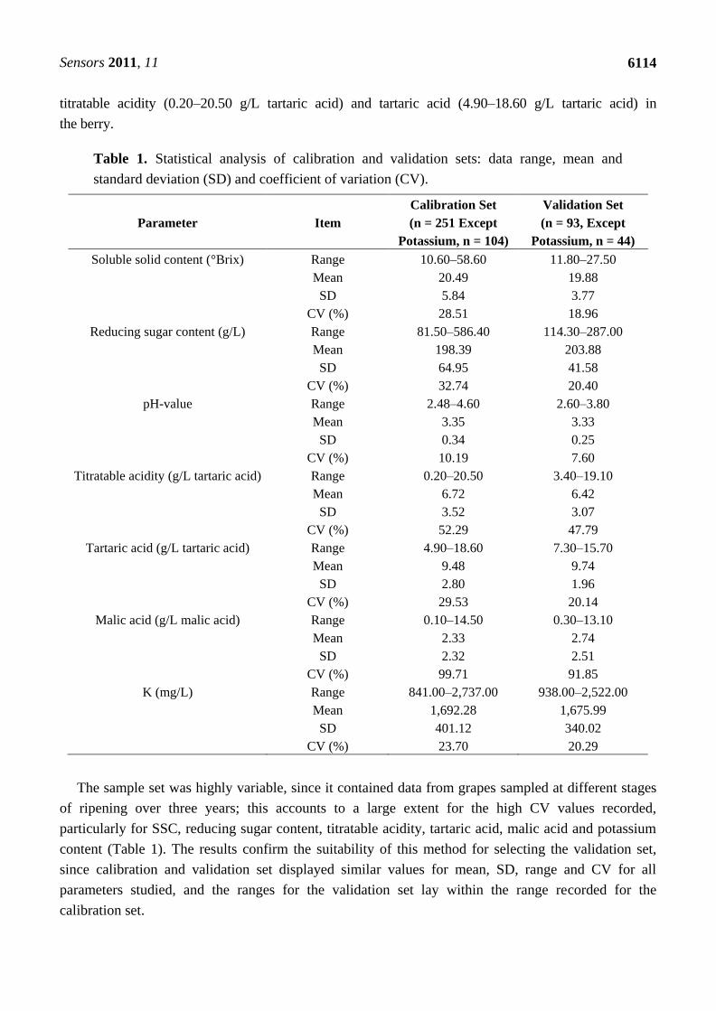
Sensors 2011, 11
6114
titratable acidity (0.20–20.50 g/L tartaric acid) and tartaric acid (4.90–18.60 g/L tartaric acid) in
the berry.
Table 1. Statistical analysis of calibration and validation sets: data range, mean and
standard deviation (SD) and coefficient of variation (CV).
Parameter Item
Calibration Set
(n = 251 Except
Potassium, n = 104)
Validation Set
(n = 93, Except
Potassium, n = 44)
Soluble solid content (°Brix) Range 10.60–58.60 11.80–27.50
Mean 20.49 19.88
SD 5.84 3.77
CV (%) 28.51 18.96
Reducing sugar content (g/L) Range 81.50–586.40 114.30–287.00
Mean 198.39 203.88
SD 64.95 41.58
CV (%) 32.74 20.40
pH-value Range 2.48–4.60 2.60–3.80
Mean 3.35 3.33
SD 0.34 0.25
CV (%) 10.19 7.60
Titratable acidity (g/L tartaric acid) Range 0.20–20.50 3.40–19.10
Mean 6.72 6.42
SD 3.52 3.07
CV (%) 52.29 47.79
Tartaric acid (g/L tartaric acid) Range 4.90–18.60 7.30–15.70
Mean 9.48 9.74
SD 2.80 1.96
CV (%) 29.53 20.14
Malic acid (g/L malic acid) Range 0.10–14.50 0.30–13.10
Mean 2.33 2.74
SD 2.32 2.51
CV (%) 99.71 91.85
K (mg/L) Range 841.00–2,737.00 938.00–2,522.00
Mean 1,692.28 1,675.99
SD 401.12 340.02
CV (%) 23.70 20.29
The sample set was highly variable, since it contained data from grapes sampled at different stages
of ripening over three years; this accounts to a large extent for the high CV values recorded,
particularly for SSC, reducing sugar content, titratable acidity, tartaric acid, malic acid and potassium
content (Table 1). The results confirm the suitability of this method for selecting the validation set,
since calibration and validation set displayed similar values for mean, SD, range and CV for all
parameters studied, and the ranges for the validation set lay within the range recorded for the
calibration set.

Sensors 2011, 11
6115
During veraison and until ripening, there is a progressive decline in malic, and to a lesser extent in
tartaric acid levels. Flanzy [3] notes that tartaric acid is mostly formed in growing organs and cannot
be metabolized except at temperatures over 35 °C. Since temperatures are highest at the end of
ripening, it is at this stage when the lowest tartaric acid levels are recorded. Malic acid is synthesized
following the combustion of sugars in chlorophyll-containing tissues. Unlike tartaric acid, it is
unstable, and is metabolized during ripening, leading to low levels at harvest.
Potassium is the major mineral cation in grapes and plays a major role in the neutralization of
tartaric and malic acid in the berries, thereby affecting the grape‘s acid profile [27,28]. Potassium
directly determines the pH not only of wine but also of must [29]. It is present in wines mainly as
potassium bitartrate, an unstable compound that can precipitate at cool temperatures as a crystalline
deposit [30].
3.2. Calibration Development using MPLS Regression and NIR Spectra
3.2.1. Prediction of Sugar-Related Quality Parameters in Grapes
Table 2 shows the best calibration models obtained using the global set (n = 251) for the prediction
of SSC and reducing sugar content according to the spectral range and derivative treatment used, for
bunches and musts, using the MPLS algorithm.
The equation displaying the greatest predictive capacity for SSC in bunches was that obtained over
the broadest spectral range, i.e., 380–1,650 nm, with statistical values of r2 = 0.94; SECV = 1.00 °Brix;
RPD = 4.12; CV = 5.08%. The predictive capacity of this equation was slightly poorer than that of the
equation obtained with grape must (RPD = 4.29; CV = 4.81%). However, both models displayed
excellent predictive capacity in term of the criteria outlined by Williams [31], who suggest than an r2
value greater than 0.9 and RPD values greater than 3 indicate excellent quantitative information.
For reducing sugar content, the equation displaying the greatest predictive capacity in bunches was
obtained over the range 780–1,650 mm, yielding statistical values for r2, SECV and RPD slightly
higher than those obtained for must samples. The RPD value (3.95) together with the r2 value (0.94)
for bunches demonstrated the robustness and power of the calibration models.
No previously-published studies address the direct measurement of SSC in bunches, and values
reported for measurements in berries tend to be lower than those obtained here; Larraín [13], for
example, recorded an RPD value of 3.40. Kemps [10] reported a RPD value of 5.05 when measuring
sugar concentrations in grape berries.
The literature contains only one report evaluating the use of NIRS to measure internal sugar-related
quality parameters in grape bunches [7]. The results obtained for SSC (r2 = 0.89; SECV = 1.41 °Brix;
RPD = 2.92) and reducing sugar content (r2 = 0.87; SECV = 17.13 g/L; RPD = 2.77) were lower than
those recorded here, confirming the need to work with broad-based sample sets which reflect
existing variability, with a view to increasing model robustness and precision. Williams [31] and
Pérez-Marín [32] highlight the importance of both sample set size and sample distribution within the
calibration set, noting that sample sets for calibration should ideally ensure uniform distribution of
composition across the range of the study parameter in question.

Sensors 2011, 11
6116
Table 2. Calibration statistics for the models obtained for predicting soluble solid content
(SSC), reducing sugar content, pH-value, titratable acidity, tartaric acid, malic acid and
potassium content for the different sample presentations and spectral ranges studied
(calibration set, n = 251 samples except for potassium cation, n = 104) using MPLS
regression.
Parameter Sample
Presentation
Spectral
Range
(nm)
Mathematic
Treatment Mean
1 SD
2 SEC
3 R
2 4 SECV
5 r
2 6 RPD
7 CV(%)
8
SSC (°Brix) Bunch 380–1,650 2,5,5,1 19.71 4.13 0.74 0.97 1.00 0.94 4.12 5.08
Must 780–1,650 1,10,5,1 19.92 4.11 0.86 0.96 0.96 0.95 4.29 4.81*
Reducing
sugar content
(g/L)
Bunch 780–1,650 2,5,5,1 191.72 53.80 10.76 0.96 13.63 0.94 3.95 7.11*
Must 380–1,650 2,5,5,1 195.48 51.14 12.00 0.94 15.36 0.91 3.33 7.86
pH-value Bunch 380–1,650 1,10,5,1 3.34 0.33 0.10 0.91 0.12 0.87 2.73 3.60*
Must 380–1,650 1,5,5,1 3.36 0.34 0.20 0.65 0.21 0.60 1.58 6.39
Titratable
acidity (g/L
tartaric acid)
Bunch 380–1,650 1,10,5,1 6.11 2.57 0.96 0.86 1.07 0.83 2.40 17.49*
Must 380–1,650 1,5,5,1 5.94 2.48 0.82 0.89 1.11 0.80 2.24 18.62
Tartaric acid
(g/L tartaric
acid)
Bunch 380–1,650 1,10,5,1 9.20 2.49 1.08 0.81 1.18 0.78 2.11 12.78*
Must 380–1,650 1,5,5,1 8.90 2.36 1.21 0.74 1.28 0.71 1.85 14.35
Malic acid
(g/L malic
acid)
Bunch 380–1,650 2,5,5,1 1.86 1.57 0.68 0.82 0.81 0.73 1.94 43.48
Must 380–1,650 2,10,5,1 1.85 1.57 0.56 0.87 0.74 0.78 2.13 39.69*
K (mg/L) Bunch 380–1,650 1,5,5,1 1,634.35 324.74 193.06 0.65 242.26 0.44 1.34 14.82*
Must 380–1,650 1,5,5,1 1,676.75 319.49 242.97 0.42 258.94 0.35 1.23 15.44 1 mean of the calibration set; 2 standard deviation; 3 standard error of calibration; 4 coefficient of
determination of calibration; 5 standard error of cross validation; 6 r2: coefficient of determination of cross
validation; 7 ratio SD/SECV; 8 coefficient of variation; * best equation.
3.2.2. Prediction of Acidity-Related Quality Parameters in Grapes
For pH-value, the best statistics (r2 = 0.87; SECV = 0.12; RPD = 2.73) for bunch analysis were
obtained with the first derivative treatment in the spectral range 380–1,650 nm (Table 2). The value
obtained for r2 (0.87) would, according to the guidelines put forward by Williams [31], provide
sufficiently good quantitative information to enable the classification of musts obtained from these
grapes, thus allowing musts to be adjusted prior to fermentation. Interestingly, bunch analysis yielded
better results than must presentation for pH-value: RPD = 2.73 and CV = 3.60% for bunch mode and
RPD = 1.58 and CV = 6.39% for must presentation.
The results obtained using bunch analysis were better than those obtained by González-Caballero [7]
(r2 = 0.69; SECV = 0.19; RPD = 1.81), by Cozzolino [33] (RPD = 1.4) and by Larraín [13] (RPD = 2.2);
in both these studies, samples were presented in berry form.
Models constructed to predict other acidity-related parameters in bunches (Table 2) may be
considered good, as indicated by the values obtained for the determination coefficient (r2 = 0.83 for
titratable acidity; r2 = 0.78 for tartaric acid; and r
2 = 0.73 for malic acid) [31]. It should also be stressed
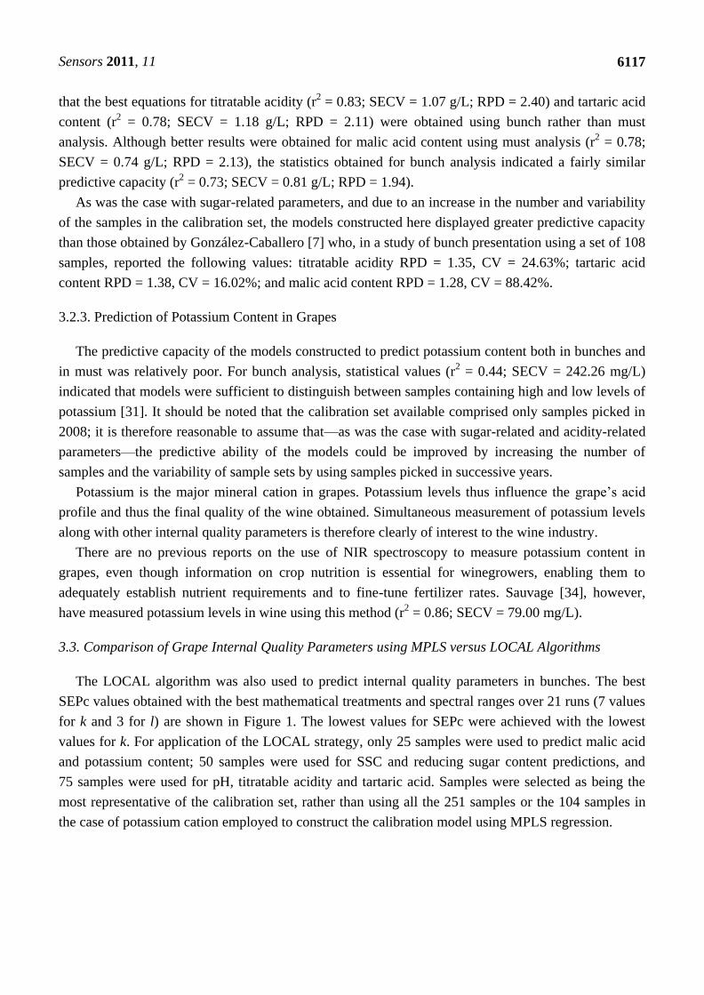
Sensors 2011, 11
6117
that the best equations for titratable acidity (r2 = 0.83; SECV = 1.07 g/L; RPD = 2.40) and tartaric acid
content (r2 = 0.78; SECV = 1.18 g/L; RPD = 2.11) were obtained using bunch rather than must
analysis. Although better results were obtained for malic acid content using must analysis (r2 = 0.78;
SECV = 0.74 g/L; RPD = 2.13), the statistics obtained for bunch analysis indicated a fairly similar
predictive capacity (r2 = 0.73; SECV = 0.81 g/L; RPD = 1.94).
As was the case with sugar-related parameters, and due to an increase in the number and variability
of the samples in the calibration set, the models constructed here displayed greater predictive capacity
than those obtained by González-Caballero [7] who, in a study of bunch presentation using a set of 108
samples, reported the following values: titratable acidity RPD = 1.35, CV = 24.63%; tartaric acid
content RPD = 1.38, CV = 16.02%; and malic acid content RPD = 1.28, CV = 88.42%.
3.2.3. Prediction of Potassium Content in Grapes
The predictive capacity of the models constructed to predict potassium content both in bunches and
in must was relatively poor. For bunch analysis, statistical values (r2 = 0.44; SECV = 242.26 mg/L)
indicated that models were sufficient to distinguish between samples containing high and low levels of
potassium [31]. It should be noted that the calibration set available comprised only samples picked in
2008; it is therefore reasonable to assume that—as was the case with sugar-related and acidity-related
parameters—the predictive ability of the models could be improved by increasing the number of
samples and the variability of sample sets by using samples picked in successive years.
Potassium is the major mineral cation in grapes. Potassium levels thus influence the grape‘s acid
profile and thus the final quality of the wine obtained. Simultaneous measurement of potassium levels
along with other internal quality parameters is therefore clearly of interest to the wine industry.
There are no previous reports on the use of NIR spectroscopy to measure potassium content in
grapes, even though information on crop nutrition is essential for winegrowers, enabling them to
adequately establish nutrient requirements and to fine-tune fertilizer rates. Sauvage [34], however,
have measured potassium levels in wine using this method (r2 = 0.86; SECV = 79.00 mg/L).
3.3. Comparison of Grape Internal Quality Parameters using MPLS versus LOCAL Algorithms
The LOCAL algorithm was also used to predict internal quality parameters in bunches. The best
SEPc values obtained with the best mathematical treatments and spectral ranges over 21 runs (7 values
for k and 3 for l) are shown in Figure 1. The lowest values for SEPc were achieved with the lowest
values for k. For application of the LOCAL strategy, only 25 samples were used to predict malic acid
and potassium content; 50 samples were used for SSC and reducing sugar content predictions, and
75 samples were used for pH, titratable acidity and tartaric acid. Samples were selected as being the
most representative of the calibration set, rather than using all the 251 samples or the 104 samples in
the case of potassium cation employed to construct the calibration model using MPLS regression.

Sensors 2011, 11
6118
Figure 1. Best SEPc values for the prediction of quality parameters in intact grapes using
the LOCAL algorithm for the different selected samples values (k), PLS factors (l), the best
mathematic treatments developed and spectral ranges. ( ) 14 PLS factors; ( ) 15 PLS
factors, ( ) 16 PLS factors).
14.5
15.0
15.5
16.0
16.5
17.0
17.5
0 25 50 75 100 125 150 175
SE
PC
Selected samples (k)
Reducing sugars content (g/L)
14
15
16
Math treatment: 2, 10, 5, 1Spectral range: 780-1650 nm
1.30
1.35
1.40
1.45
1.50
1.55
0 25 50 75 100 125 150 175
SE
PC
Selected samples (k)
Soluble solid content (ºBrix)
14
15
16
Math treatment: 2, 10, 5, 1Spectral range: 780-1650 nm
1.75
1.80
1.85
1.90
1.95
2.00
0 25 50 75 100 125 150 175
SE
PC
Selected samples (k)
Titrable acidity (g/L tartaric acid)
14
15
16
Math treatment: 1, 10, 5, 1Spectral range: 780-1650 nm
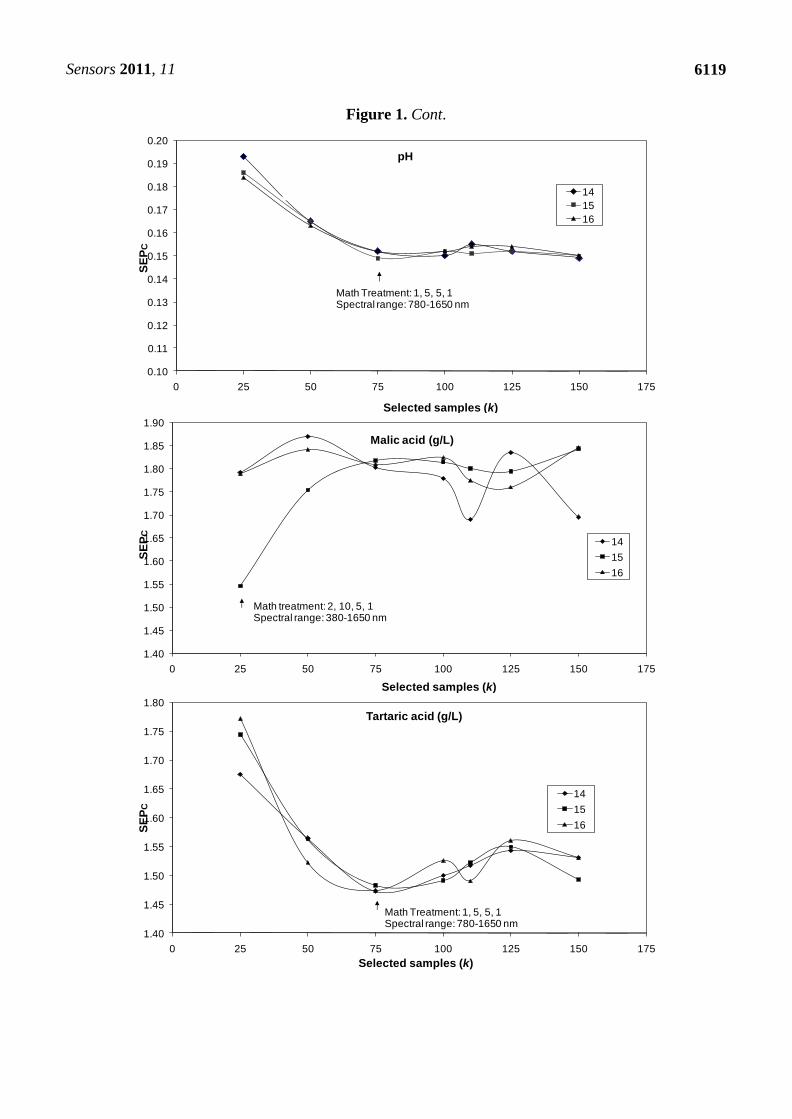
Sensors 2011, 11
6119
Figure 1. Cont.
0.10
0.11
0.12
0.13
0.14
0.15
0.16
0.17
0.18
0.19
0.20
0 25 50 75 100 125 150 175
SE
PC
Selected samples (k)
pH
14
15
16
Math Treatment: 1, 5, 5, 1Spectral range: 780-1650 nm
1.40
1.45
1.50
1.55
1.60
1.65
1.70
1.75
1.80
1.85
1.90
0 25 50 75 100 125 150 175
SE
PC
Selected samples (k)
Malic acid (g/L)
14
15
16
Math treatment: 2, 10, 5, 1Spectral range: 380-1650 nm
1.40
1.45
1.50
1.55
1.60
1.65
1.70
1.75
1.80
0 25 50 75 100 125 150 175
SE
PC
Selected samples (k)
Tartaric acid (g/L)
14
15
16
Math Treatment: 1, 5, 5, 1Spectral range: 780-1650 nm

Sensors 2011, 11
6120
Figure 1. Cont.
In most cases, the values selected for parameter l (number of PLS terms) had little influence on
SEPc values; marked differences being observed only for SSC and malic acid. The best results
achieved with the LOCAL algorithm were then compared with those obtained using MPLS regression
for the prediction of the 93-sample validation set except for the potassium cation (n = 44), using only
bunch analysis (Table 3).
It needs to point out that the sistematic procedure follows in this work is more favourable for the
LOCAL algorithm, since the tuning of LOCAL was done on the validation set, with 21 combinations
of parameters, being selected the one with best SEP, while the best MPLS model was chosen taking
into account the cross validation statistics and only the best model applied to the validation set.
Nevertheless, this systematic has been selected since the differences between the statistics obtained for
the MPLS models were no-relevant, and also taking into account that cross-validation statistics,
according to Shenk [23], give a realistic estimate of the error prediction of samples not included in the
calibration.
The results obtained using LOCAL were better than those achieved using MPLS regression, in
terms of both r2 and SEPc, for total soluble solid content, reducing sugar content, pH, tartaric acid and
potassium content, although the improvement was only slight for reducing sugar and tartaric acid
content. For titratable acid and malic acid, application of the LOCAL algorithm improved model
precision but also prompted a slight increase in SEPc values.
The improvement in r2 values achieved using the non-linear strategy ranged between 2% for both
tartaric acid and reducing sugar content and 41% for malic acid, while the improvement in SEPc
values ranged from 1.5% for tartaric acid to 22% for SSC. Shenk [35] suggest that application of the
LOCAL algorithm can improve the predictive capacity of models by 10–30%.
With regard to spectral range suitability, the best results using the LOCAL strategy were generally
obtained in the 780–1,650 nm range, except for malic acid content; by contrast, MPLS yielded the best
results for all parameters using a wider spectral range (380–1,650 nm), except for reducing sugar
content. The optimal number of PLS terms for the prediction of each parameter using the LOCAL
algorithm (Table 3) was always equal to or smaller than the optimal number using MPLS.
250
270
290
310
330
350
370
0 25 50 75 100
SE
Pc
Selected samples (k)
Potassium catium (mg/L)
14
15
16
Math treatment: 2, 5, 5, 1Spectral range: 780-1650 nm

Sensors 2011, 11
6121
Table 3. Validation statistics for the best models for predicting soluble solid content
(SSC), reducing sugar content, pH-value, titratable acidity, tartaric acid, malic acid and
potassium content using MPLS and LOCAL algorithms.
Parameter Method Mathematic
Treatment
Spectral
Region Factors SEP
1 SEPc
2 Bias r
2 3 Slope
SSC (°Brix) MPLS 2,5,5,1 380–1,650 16 1.69 1.69 0.17 0.80 0.97
LOCAL (k = 50) 2,10,5,1 780–1,650 16 (−4) 1.33 1.32 0.24 0.88 0.96
Reducing sugar
content (g/L)
MPLS 2,5,5,1 780–1,650 16 16.67 15.80 5.57 0.86 0.94
LOCAL (k = 50) 2,10,5,1 780–1,650 14 (−4) 16.40 15.02 6.77 0.88 0.91
pH-value MPLS 1,10,5,1 380–1,650 16 0.17 0.17 0.02 0.58 0.84
LOCAL (k = 75) 1,5,5,1 780–1,650 15 (−4) 0.15 0.15 0.02 0.66 1.11
Titratable
acidity (g/L
tartaric acid)
MPLS 1,10,5,1 380–1,650 16 1.73 1.67 −0.49 0.48 0.85
LOCAL (k = 75) 1,10,5,1 780–1,650 16 (−4) 1.87 1.80 −0.54 0.66 0.97
Tartaric acid
(g/L tartaric
acid)
MPLS 1,10,5,1 380–1,650 16 1.60 1.49 0.60 0.46 0.88
LOCAL (k = 75) 1,5,5,1 780–1,650 14 (−4) 1.47 1.47 0.08 0.47 0.79
Malic acid (g/L
malic acid)
MPLS 2,5,5,1 380–1,650 16 1.39 1.39 0.20 0.30 0.95
LOCAL (k = 25) 2,10,5,1 380–1,650 15 (−4) 1.54 1.55 −0.02 0.51 0.89
K (mg/L) MPLS 1,5,5,1 380–1,650 14 300.23 301.15 −38.83 0.29 0.67
LOCAL (k = 25) 2,5,5,1 780–1,650 14 (−4) 284.52 281.71 −69.02 0.39 0.80 1 standard error of prediction; 2 standard error of prediction bias-corrected; 3 coefficient of determination of
prediction.
4. Conclusions
The results obtained here when analyzing grapes in bunch form—a method that requires no
previous sample preparation—confirm that NIRS technology is well suited for evaluating internal
quality characteristics related to sugar content and acidity, for the non-destructive quantification of
chemical changes taking place during on-vine ripening, and for deciding on the optimum time for
harvesting. NIR technology additionally enables the classification of bunches in terms of low versus
and high potassium levels, using a very fast, non-destructive sensor.
The results also highlight the need to develop models using a database sufficiently large to reflect
the spectral variability that may be encountered during on-vine ripening. In comparison with MPLS
regression, the LOCAL algorithm proved to be a highly effective tool for improving the prediction of
internal quality parameters in intact grapes.
Acknowledgements
This research was funded by the Andalusian Regional Government under the Research Excellence
Program (Project No. P09-AGR-5129 ―MEMS and NIRS-image sensors for the in situ non-destructive
analysis of food and feed‖).

Sensors 2011, 11
6122
References
1. Menesatti, P. In-Field Spectrophotometric Measurement to Estimate Maturity Stage of Wine
Grapes. Proc. SPIE 2007, 6761, 676118.
2. Moreno, J.; Peinado, R.A. Química Enológica; A. Madrid Vicente and Mundi-Prensa: Madrid,
Spain, 2010.
3. Flanzy, C. Enología: Fundamentos Científicos y Tecnológicos; Mundi-Prensa: Madrid, Spain,
2003.
4. Sas, A. The Missing Gap: Measuring and Paying for Grape Quality; Blair, R., Williams, P.,
Pretorius, S., Eds.; The Australian Wine Research Institute: Adelaide, Australia, 2008; pp. 52-55.
5. Fernández-Novales, J.; López, M.I.; Sánchez, M.T.; Morales, J.; González-Caballero, V.
Shortwave-Near Infrared Spectroscopy for Determination of Reducing Sugar Content during
Grape Ripening, Winemaking and Aging of White and Red Wines. Food Res. Int. 2009, 42,
285-291.
6. Fernández-Novales, J.; López, M.I.; Sánchez, M.T.; García-Mesa, J.A.; González-Caballero, V.
Assessment of Quality Parameters in Grapes during Ripening Using a Miniature Fiber-Optic
Near-Infrared Spectrometer. Int. J. Food Sci. Nutr. 2009, 60, 265-277.
7. González-Caballero, V.; Sánchez, M.T.; López, M.I.; Pérez-Marín, D. First Steps
towards the Development of a Non-Destructive Technique for the Quality Control of Wine
Grapes during On-Vine Ripening and on Arrival at the Winery. J. Food Eng. 2010,
doi:10.1016/j.jfoodeng.2010.06.016.
8. Gishen, M.; Dambergs, R.G.; Kambouris, A.; Kwiatkowski, M.; Cynkar, W.U.; Høj, P.B.
Application of Near Infrared Spectroscopy for Quality Assessment of Grapes, Wine and Spirits.
In Proceedings of 9th International Conference on Near Infrared Spectroscopy, Verona, Italy,
13–18 June 1999; pp. 917-920.
9. Herrera, J.; Guesalaga, A.; Agosin, E. Shortwave-Near Infrared Spectroscopy for Non-Destructive
Determination of Maturity of Wine Grapes. Meas. Sci. Tech. 2003, 14, 689-697.
10. Kemps, B.; León, L.; Best, S.; De Baerdemaeker, J.; De Ketelaere, B. Assessment of the Quality
Parameters in Grapes using VIS/NIR Spectroscopy. Biosyst. Eng. 2010, 105, 507-513.
11. Cozzolino, D.; Dambergs, R.G.; Janik, L.; Cynkar, W.U.; Gishen, M. Analysis of Grapes and
Wine by Near Infrared Spectroscopy. J. Near Infrared Spectrosc. 2006, 14, 279-289.
12. Dambergs, R.G.; Cozzolino, D.; Cynkar, W.U.; Janik, L.; Gishen, M. The Determination of Red
Grape Quality Parameters using the LOCAL Algorithm. J. Near Infrared Spectrosc. 2006, 14,
71-79.
13. Larraín, M.; Guesalaga, A.R.; Agosin, E. A Multipurpose Portable Instrument for Determining
Ripeness in Wine Grapes using NIR Spectroscopy. IEEE T. Instrument. Meas. 2008, 57, 294-302.
14. Cao, F.; Wu, D.; He, Y. Soluble solids Content and pH Prediction and Varieties Discrimination of
Grapes Based on Visible–Near Infrared Spectroscopy. Comput. Electron. Agr. 2010, 71, S15-S18.
15. Guidetti, R.; Beghi, R.; Bodria, L. Evaluation of Grape Quality Parameters by a Simple Vis/NIR
System. T. ASABE. 2010, 53, 477-484.
16. Berzaghi, P.; Shenk, J.S.; Westerhaus, M.O. LOCAL Prediction with Near Infrared Multi-Product
Databases. J. Near Infrared Spectrosc. 2000, 8, 1-9.

Sensors 2011, 11
6123
17. Shenk, J.S.; Westerhaus, M.O.; Berzaghi, P. Investigation of a LOCAL Calibration Procedure for
Near Infrared Instruments. J. Near Infrared Spectrosc. 1997, 5, 223-232.
18. Spanish Ministry of Agriculture, Fisheries and Food. Official Methods of Analysis.Vol.II;
Secretaría General de Alimentación, Dirección General de Política Alimentaria: Madrid, Spain,
1993; pp. 35-319.
19. Shenk, J.S.; Westerhaus, M.O. Population Definition Sample Selection and Calibration
Procedures for Near Infrared Spectra and Modified Partial Least Squares Regression. Crop Sci.
1991, 31, 469-474.
20. ISI. The Complete Software Solution Using a Single Screen for Routine Analysis, Robust
Calibrations, and Networking; Manual, FOSS NIRSystems/TECATOR; Infrasoft International:
Silver Spring, MD, USA, 2000.
21. Barnes, R.J.; Dhanoa, M.S.; Lister, S.J. Standard Normal Variate Transformation and
De-Trending of Near Infrared Diffuse Reflectance Spectra. Appl. Spectrosc. 1989, 43, 772-777.
22. Shenk, J.S.; Westerhaus M.O. Calibration the ISI Way. In Near Infrared Spectroscopy: The
Future Waves; Davies, A.M.C., Williams, P.C., Eds.; NIR Publications: Chichester, UK, 1996;
pp. 198-202.
23. Shenk, J.S.; Westerhaus, M.O. Analysis of Agricultural and Food Products by Near Infrared
Reflectance Spectroscopy; NIRSystems, Inc.: Silver Spring, MD, USA, 1995.
24. Dardenne, P.; Sinnaeve, G.; Baeten, V. Multivariate Calibration and Chemometrics for Near
Infrared Spectroscopy: Which Method? J. Near Infrared Spectrosc. 2000, 8, 229-237.
25. Pérez-Marín, D.; Garrido-Varo, A.; Guerrero, J.E. Non-Linear Methods in NIRS Quantitative
Analysis. Talanta 2007, 72, 28-42.
26. Barton II, F.E.; Shenk, J.S.; Westerhaus, M.O.; Funk, D.B. The Development of Near Infrared
Wheat Quality Models by Locally Weighted Regressions. J. Near Infrared Spectrosc. 2000, 8,
201-208.
27. Hidalgo, L. Tratado de Viticultura General; Mundi-Prensa Libros, S.A.: Madrid, Spain, 2004.
28. Da Mota, R.V.; De Souza, C.R.; Favero, A.C.; Silva, C.P. C.E.; Do Carmo, E.L.; Fonseca, A.R.;
Regina, M.D. Productivity and Physicochemical Composition of Berries of Grapevine Cultivars
Grafted onto Different Rootstocks. Pesqui. Agropecu. Bras. 2009, 44, 576-582.
29. González, L.A.; Armas, P.A.; González, J.E.; García, M.J.; Vidarte, E.; Pomar, M. Estudio de los
cationes sodio, potasio, hierro y cobre, durante la maduración de las cepas Listán negro, Listán
blanco y Nnegramoll. D.O.Tacoronte-Acentejo. Jornadas Técnicas Vitivinícolas Canarias 1997,
1997, 21-26.
30. Rankine, B. Making Good Wine. A Manual of Winemaking Practice for Australia and New
Zealand; Pan Macmillan: London, UK, 2004.
31. Williams, P.C. Implementation of Near-Infrared Technology. In Near-Infrared Technology in the
Agricultural and Food Industries; Williams, P.C., Norris, K.H., Eds.; AACC, Inc.: St. Paul, MN,
USA, 2001; pp. 145-169.
32. Pérez-Marín, D.; Garrido-Varo, A.; Guerrero, J.E. Implementation of LOCAL Algorithm with
Near-Infrared Spectroscopy for Compliance Assurance in Compound Feedingstuffs. Appl.
Spectrosc. 2005, 59, 69-77.

Sensors 2011, 11
6124
33. Cozzolino, D.; Esler, M.B.; Dambergs, R.G.; Cynkar, W.U.; Boehm, D.R.; Francis, I.L.;
Gishen, M. Prediction of Color and pH in Grapes using a Diode Array Spectrophotometer
(400–1,100 nm). J. Near Infrared Spectrosc. 2004, 12, 105-111.
34. Sauvage, L.; Frank, D.; Stearne, J.; Millikan, M.B. Trace Metal Studies of Selected White Wines:
An Alternative Approach. Anal. Chim. Acta 2002, 458, 223-230.
35. Shenk, J.S.; Workman, J.J., Jr.; Westerhaus, M.O. Application of NIR Spectroscopy to
Agricultural Products. In Handbook of Near Infrared Analysis, Second Edition; Practical
Spectroscopy Series; Burns, D.A., Ciurczak, E.W., Eds.; Marcel Dekker: Monticello, NY, USA,
2001; Volume 27, pp. 419-473.
© 2011 by the authors; licensee MDPI, Basel, Switzerland. This article is an open access article
distributed under the terms and conditions of the Creative Commons Attribution license
(http://creativecommons.org/licenses/by/3.0/).

NIRS para la predicción de parámetros de calidad interna y momento óptimo de cosecha en uvas y control de calidad y trazabilidad en la industria vitivinícola
______________________________________________________________________
117
4.3. ON-VINE MONITORING OF GRAPE RIPENING USING NEAR
INFRARED SPECTROSCOPY. FOOD ANALYTICAL METHODS (2012)

118

On-Vine Monitoring of Grape RipeningUsing Near-Infrared Spectroscopy
Virginia González-Caballero & María-Teresa Sánchez &
Juan Fernández-Novales & María-Isabel López &
Dolores Pérez-Marín
Received: 9 December 2011 /Accepted: 23 February 2012# Springer Science+Business Media, LLC 2012
Abstract This study evaluated the ability of near-infrared(NIR) spectroscopy to characterise the behaviour of whiteand red grapes during on-vine ripening, as a function of grapeposition in the bunch (high, middle and low) and bunchorientation (north, south, east and west) and to distinguishbetween different ripening stages with a view to optimisingharvesting times depending on the grape variety and the type ofwine to be made. A total of 24 bunches of two wine-grapevarieties (cv. Pedro Ximénez and cv. Cabernet Sauvignon)were labelled and analysed directly on the vine using a com-mercially available handheld micro-electro-mechanical systemspectrophotometer (1,600–2,400 nm). Principal componentanalysis was performed to study relationships between thevarious configurations (grape position and bunch orientation),ripening stages and spectral data. Results for the white-grapevariety showed that grapes high on the bunch behaved differ-ently during ripening from those in central or low positions andthat east-facing bunches behaved differently from the rest. Forboth varieties, analysis of bunch spectral characteristics
enabled three stages of ripening to be distinguished: early,middle and late. Subsequently, the ability of NIR technologyto classify wine grapes as a function of reducing-sugar content,with a view to optimising harvest timing, was evaluated bypartial least squares discriminant analysis: 88% of whitegrapes and 88% of red grapes were correctly classified whileover 79% of samples were correctly assigned to representativegroups. These results confirmed that NIR technology in thespectral range 1,600–2,400 nm is an appropriate technique foron-vine monitoring of the ripening process, enabling selectiveharvesting depending on the type of wine to be made.
Keywords NIR spectroscopy .Wine grape . On-vine .
Ripening . Portable sensor
Introduction
The monitoring of bunch development and of within-bunchvariations in grape composition during on-vine ripening isan essential part of ensuring high-quality wines; winemakersnearly always identify uniform batches of good-quality fruitas their main priority (Bramley 2005).
Since grape heterogeneity may influence final wine com-position and quality, it should be carefully evaluated at harvest(Kontoudakis et al. 2011). At any given date, the physiologicalcharacteristics of grape berries in a vineyard may vary consid-erably (Torchio et al. 2010).
It is equally important for winemakers to be aware of thefactors influencing harvest timing, many of which are beyondtheir control. Among the major factors are weather conditions:seasonal variations including heat waves and sudden heavyrains can be extremely detrimental to plant health and maylead to over-ripening, thus impairing final wine quality (Ruíz-Hernández 2001).
V. González-Caballero :M.-I. LópezCentro de Investigación y Formación Agraria de “Cabra-Priego”,Instituto de Investigación y Formación Agraria y Pesquera(IFAPA), Consejería de Agricultura y Pesca, Junta de Andalucía,Cabra, Córdoba, Spain
M.-T. Sánchez (*) : J. Fernández-NovalesDepartment of Bromathology and Food Technology,University of Cordoba, Campus of Rabanales,14071 Cordoba, Spaine-mail: [email protected]
D. Pérez-Marín (*)Department of Animal Production,University of Cordoba, Campus Rabanales,14071 Cordoba, Spaine-mail: [email protected]
Food Anal. MethodsDOI 10.1007/s12161-012-9389-3
Author's personal copy

At present, grape ripeness is mostly evaluated by labora-tory analysis, using traditional physical/chemical methods totest representative grape samples obtained at regular inter-vals throughout the ripening period (Krstic et al. 2003; Ilandet al. 2004). Analysis is aimed primarily at measuring sugarcontent, titratable acidity and malic acid content; secondarymeasurements include pH, 100-berry weight and tartaricacid content. The sample used has to be representative, i.e.it should provide the results that would be obtained if thewhole plot were to be harvested at the same time (Blouinand Guimberteau 2000). In order to ensure representativity,measurements should be made on bunches selected alter-nately from sunny and shady positions and on berries takenfrom the outer and inner areas of the bunch (Moreno andPeinado 2010). However, laboratory analysis is still some-thing of a bottleneck for the proper estimation of grapestatus, and there are a few published studies on variationsin grape composition within a single bunch, due largely todata-collection constraints (Ben Ghozlen et al. 2010).
Visual inspection of bunches throughout ripening and upuntil harvest shows that berry colour changes considerably asa function of bunch position on the vine; even within a singlebunch, berry colour may vary substantially depending on thedegree of exposure to the sun (Blouin and Guimberteau 2000).Moreover, sugar content is highest on grapes growing higheron the bunch, close to the stalk, and gradually declines downthe bunch; acid content displays the reverse pattern (Hidalgo2006).
Of the various analytical techniques available, near-infrared (NIR) spectroscopy has shown considerable potentialfor the non-destructive measurement of internal attributes andripeness in fruits (Nicolaï et al. 2007; Sánchez and Pérez-Marín 2011). Over the last few years, moreover, the develop-ment of handheld near-infrared devices has enhanced thepotential of NIR spectroscopy for the in situ monitoring andanalysis of the fruit ripening process (Pérez-Marín et al. 2009;Sánchez et al. 2011).
However, no published studies have yet focused on theuse of miniaturised, handheld, near-infrared devices basedon micro-electro-mechanical system (MEMS) technology ingrapes as a means of characterising variations in on-vineripening as a function of grape position and bunch orienta-tion, with a view to optimising harvesting times and thusenabling selective harvesting depending on the type of wineto be made. This was the purpose of the present study.
Materials and Methods
Grape Sampling During Ripening
The experiment was carried out in 2008, in a vineyard belong-ing to the Agricultural Research and Training Centre in Cabra
(Cordoba, Spain). Two grape (Vitis vinifera L.) varieties wereselected: one white (cv. Pedro Ximénez) and one red (cv.Cabernet Sauvignon), both grown under regulated deficitirrigation. For each variety, two bunches were selected fromeach of six selected vines, giving a total of 24 bunches (12white and 12 red). Bunches were labelled and analysed byNIR spectroscopy on the vine throughout the ripening process.
Spectrum collection started on 20 August. On-vine meas-urements were made every 3 or 4 days (except for thesecond measurement, which was made 6 days after the first)until harvest (9 Sept); a total of six measurements weremade during the ripening process. NIR spectra were cap-tured from samples taken from selected bunches using thehandheld MEMS spectrometer; bunches from adjacent vineswere then collected for physical–chemical analysis, in orderto provide reference values for the properties measured. Onarrival at the laboratory, grapes were promptly placed inrefrigerated storage at 0 °C and 95% relative humidity. Priorto each physical–chemical measurement, samples wereallowed to stabilise at laboratory temperature (25 °C).
Spectra Collection
Spectra were collected on grapes in reflectance mode (log 1/R)using a handheldMEMS spectrometer (Phazir 2400, Polychro-mix, Inc., Wilmington, MA, USA). The Phazir 2400 is anintegrated near-infrared handheld analyser that incorporatesall the essential components to deliver on-vine applications(Geller and Ramani 2005). The spectrophotometer scans at8-nm intervals (pixel resolution, 8 nm and optical resolution,12 nm), across a range of NIR wavelengths from 1,600 to2,400 nm. Sensor integration time is 600 ms.
Each of the twelve bunches selected for each variety wasdivided into three areas (high, middle and low), and fourspectra were captured for each area to reflect orientation(north, south, east and west).
Since measurements were made on the vine, sampletemperature was not controlled beforehand; mean tempera-ture on measurement days ranged from 22 to 29 °C. Spectralacquisition was performed in sunlight, i.e. no light-tight boxwas used.
Reference Data Analysis
Immediately after sampling, berries from adjacent vineswere weighed on an electronic balance (0–320±0.0001 g;model C600-SX, Cobos, Barcelona, Spain) to determine theaverage 100-berry weight. Samples were then analysed forsoluble solids content, reducing-sugar content, pH value,titratable acidity, tartaric acid and malic acid contents.
For this purpose, berries were passed through a hand-operated food mincer, which enabled constant pressure to bemaintained during juice extraction with minimal seed and
Food Anal. Methods
Author's personal copy
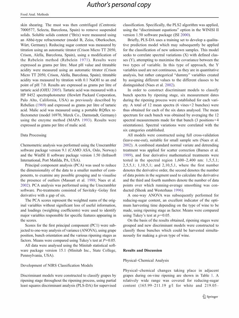
skin shearing. The must was then centrifuged (Centronic7000577, Selecta, Barcelona, Spain) to remove suspendedsolids. Soluble solids content (°Brix) were measured usingan Abbé-type refractometer (model B, Zeiss, Oberkochen,Würt, Germany). Reducing sugar content was measured bytitration using an automatic titrator (Crison Micro TT 2050,Crison, Alella, Barcelona, Spain), using a modification ofthe Rebelein method (Rebelein 1971). Results wereexpressed as grams per litre. Must pH value and titratableacidity were measured using an automatic titrator (CrisonMicro TT 2050, Crison, Alella, Barcelona, Spain); titratableacidity was measured by titration with 0.1 NaOH to an endpoint of pH 7.0. Results are expressed as grams per litre oftartaric acid (OJEU 2005). Tartaric acid was measured with aHP 8452 spectrophotometer (Hewlett Packard Corporation,Palo Alto, California, USA) as previously described byRebelien (1969) and expressed as grams per litre of tartaricacid. Malic acid was measured using a portable RQflex re-flectometer (model 16970, Merck Co., Darmstadt, Germany)using the enzyme method (MAPA 1993). Results wereexpressed as grams per litre of malic acid.
Data Processing
Chemometric analysis was performed using the Unscramblersoftware package version 9.1 (CAMO ASA, Oslo, Norway)and the WinISI II software package version 1.50 (InfrasoftInternational, Port Matilda, PA, USA).
Principal component analysis (PCA) was used to reducethe dimensionality of the data to a smaller number of com-ponents, to examine any possible grouping and to visualisethe presence of outliers (Massart et al. 1988; Naes et al.2002). PCA analysis was performed using the Unscramblersoftware. Pre-treatments consisted of Savitzky–Golay firstderivative with a gap of six.
The PCA scores represent the weighted sums of the orig-inal variables without significant loss of useful information,and loadings (weighting coefficients) were used to identifymajor variables responsible for specific features appearing inthe scores.
Scores for the first principal component (PC1) were sub-jected to one-way analysis of variance (ANOVA), using grapeposition, bunch orientation and the various ripening stages asfactors. Means were compared using Tukey’s test at P00.05.
All data were analysed using the Minitab statistical soft-ware package version 15.1 (Minitab Inc., State College,Pennsylvania, USA).
Development of NIRS Classification Models
Discriminant models were constructed to classify grapes byripening stage throughout the ripening process, using partialleast squares discriminant analysis (PLS-DA) for supervised
classification. Specifically, the PLS2 algorithm was applied,using the “discriminant equations” option in the WINISI IIversion 1.50 software package (ISI 2000).
Briefly, PLS-DA uses a training set to develop a qualita-tive prediction model which may subsequently be appliedfor the classification of new unknown samples. This modelseeks to correlate spectral variations (X) with defined clas-ses (Y), attempting to maximise the covariance between thetwo types of variable. In this type of approach, the Yvariables used are not continuous, as they are in quantitativeanalysis, but rather categorical “dummy” variables createdby assigning different values to the different classes to bedistinguished (Naes et al. 2002).
In order to construct discriminant models to classifybunch spectra by ripening stage, six measurement datesduring the ripening process were established for each vari-ety. A total of 12 mean spectra (6 vines×2 bunches) werethus obtained for each of the six dates analysed. The meanspectrum for each bunch was obtained by averaging the 12spectral measurements made for that bunch (3 positions×4orientations). Spectral variations were correlated with thesix categories established.
All models were constructed using full cross-validation(leave-one-out), suitable for small sample sets (Naes et al.2002). A combined standard normal variate and detrendingtreatment was applied for scatter correction (Barnes et al.1989), and four derivative mathematical treatments weretested in the spectral region 1,600–2,400 nm: 1,5,5,1;2,5,5,1; 1,10,5,1; and 2,10,5,1, where the first numberdenotes the derivative order, the second denotes the numberof data points in the segment used to calculate the derivativeand the third and fourth numbers denote the number of datapoints over which running-average smoothing was con-ducted (Shenk and Westerhaus 1996).
A one-way ANOVA was subsequently performed forreducing-sugar content, an excellent indicator of the opti-mum harvesting time depending on the type of wine to bemade, using ripening stage as factor. Means were comparedusing Tukey’s test at p00.05.
On the basis of the results obtained, ripening stages weregrouped and new discriminant models were constructed toclassify those bunches which could be harvested simulta-neously for making a given type of wine.
Results and Discussion
Physical–Chemical Analysis
Physical–chemical changes taking place in adjacentgrapes during on-vine ripening are shown in Table 1. Arelatively wide range was covered for reducing-sugarcontent (165.99–211.19 g/l for white and 219.05–
Food Anal. Methods
Author's personal copy

268.80 g/l for red grapes) since sampling was carried outsimultaneously for the two varieties throughout the rip-ening process.
Towards the end of veraison, a rapid berry-growth phaseis observed due to cell enlargement prompted by the swiftdevelopment of grape physical–chemical characteristics(Table 1). This is accompanied by a progressive increasein reducing-sugar content in vine shoots, leaves and fruits(Reynier 2003). Sugar content increases very rapidly in theberry during ripening, but the rate of increase slows down asripening progresses, and stabilises at the moment of fullripeness; absolute values may even fall thereafter when theberry becomes overripe (Hidalgo 2006.)
Although the two varieties clearly differed in 100-berryweight and thus in berry size, trends over the ripening periodwere very similar. Red grape varieties tend to have a greaternumber of berries per bunch, thus favouring the steepingprocess during alcoholic fermentation, and 100-berry weightis considerably lower than for white varieties (Table 1).
Analysis of reducing-sugar content showed that ‘PedroXiménez’ grapes exhibited a ripening pattern different fromthat of ‘Cabernet Sauvignon’ grapes: at the start of the study,which was performed simultaneously for the two varieties,‘Cabernet Sauvignon’ grapes were already approaching thefinal stage of ripeness, and sugar accumulation during thestudy period was comparatively slight. By contrast, ‘PedroXiménez’—a later variety—displayed the typical rise inreducing-sugar content during the early stages of ripening,although the last two measurements were affected by rainfall,and the ripeness levels expected for making Fino wines in theMontilla-Moriles region (Córdoba) were not in fact attained.
The optimal harvesting time for ‘Cabernet Sauvignon’grapes used for making high-quality red wines is based on
an optimal balance of sugar content, colour, aromas andacidity. The best time for harvesting ‘Pedro Ximénez’grapes, used for making high-quality young white wines,is the point of maximum aroma and acidity; this is usuallyachieved by earlier harvesting (Martínez-Valero et al. 2001).However, the same variety is also used for making Finowines, for which the main requirement is a high reducing-sugar content (above 244 g/l); this is achieved by laterharvesting. In order to determine the optimal harvestingtime, it is therefore essential to analyse bunch ripening witha view to charting changes in major components.
Fluctuations in acidity-related parameters (titratable acid-ity, tartaric and malic acid content) were due to a decline ingrape acidity during ripening, as a result of the migration orconsumption and dilution of these two predominant acids(Blouin and Cruege 2003). After veraison, tartaric acidcontent decreased only slightly, remaining virtually constantfor both varieties, since variations in temperature during theripening period were offset by vine water availability(Table 1). High temperatures tend to prompt increased res-piratory combustion of tartaric acid, while the presence ofmoisture increases the levels of this acid in the bunch(Hidalgo 2006). By contrast, malic acid levels fell steadilythroughout ripening, displaying a more marked declinewhen external temperatures were higher (López et al.2009) (Table 1).
Influence of Position, Orientation and Ripening Stageon Bunch Ripeness
Principal component analysis was performed to examine therelationship between the various configurations of bunchorientation and grape position and ripening stages and the
Table 1 Physical–chemical changes in ‘Pedro Ximénez’ and ‘Cabernet Sauvignon’ adjacent grapes during ripening
Variety Ripeningstage
Date 100-berryweight (g)
SSC(°Brix)
Reducing-sugarcontent (g/l)
pHvalue
Titratable acidity(g/l tartaric acid)
Tartaric acid(g/l tartaric acid)
Malic acid(g/l malic acid)
Pedro Ximénez M1 20 Aug 189.75 16.40 165.99 3.21 7.50 8.60 2.42
M2 26 Aug 184.25 17.15 175.54 3.38 6.16 8.55 1.85
M3 29 Aug 189.72 19.95 202.19 3.36 7.08 7.89 0.90
M4 02 Sep 192.45 20.40 211.19 3.49 3.77 8.29 1.26
M5 05 Sep 204.43 18.75 189.03 3.34 4.15 8.91 1.39
M6 09 Sep 215.06 17.40 173.28 3.43 4.18 8.04 1.42
Cabernet Sauvignon M1 20 Aug 80.79 21.50 219.05 3.30 4.50 11.01 3.30
M2 26 Aug 63.77 24.10 246.53 3.49 5.30 9.06 3.00
M3 29 Aug 66.78 26.00 262.88 3.49 4.23 7.71 2.80
M4 02 Sep 71.78 26.25 268.80 3.55 4.92 9.15 2.73
M5 05 Sep 82.36 24.30 249.94 3.50 4.59 8.59 2.71
M6 09 Sep 88.25 23.80 239.81 3.59 4.29 9.39 2.36
SSC soluble solids content
Food Anal. Methods
Author's personal copy
spectral measurements recorded during on-vine ripening ofred and white grapes.
Score plots for ‘Pedro Ximénez’ grapes are shown inFig. 1. The first two principal components accounted for ahigh degree of variance (80.18 and 6.47%, respectively). Inthese plots, no grouping of samples by grape position (high,middle and low), by bunch orientation (north, south, eastand west) or even by ripening stage (stages 1 to 6) wereapparent.
For ‘Cabernet Sauvignon’ grapes (data not shown), the firsttwo principal components together accounted for 93.28% oftotal variance; PC1 accounted for 86.13% and PC2 for 7.15%.
Analysis revealed no apparent grouping by position, orienta-tion or ripening stage.
Loadings (weighting coefficients) for the two first principalcomponents (Fig. 2) in both grape varieties showed that thekey wavelengths for distinguishing between ripening stageswere associated with the first sugar-related overtone at around1,750 and 2,067 nm and with water peaks at around 1,900 and1,970 nm (Williams 2001).
A statistical analysis was carried out in order to identifypossible significant differences attributable to these three fac-tors in both varieties throughout ripening. One-way ANOVAwas performed on the first principal component for ‘Pedro
Grape Position
-0.02
-0.01
-0.01
0.00
0.01
0.01
0.02
-0.03 -0.02 -0.01 0.00 0.01 0.02 0.03 0.04
-0.03 -0.02 -0.01 0.00 0.01 0.02 0.03 0.04
PC 1 (80.18%)
PC
2 (
6.47
%)
H1 H2 H3 H4 H5 H6 M1 M2 M3
M4 M5 M6 L1 L2 L3 L4 L5 L6
Bunch Orientation
-0.02
-0.01
-0.01
0.00
0.01
0.01
0.02
PC 1 (80.18%)
PC
2 (
6.47
%)
E1 E2 E3 E4 E5 E6 N1 N2 N3 N4 N5 N6
W1 W2 W3 W4 W5 W6 S1 S2 S3 S4 S5 S6
Fig. 1 Principal componentanalysis for bunchconfiguration during ripening in‘Pedro Ximénez’ grapes
Food Anal. Methods
Author's personal copy

Ximenez’ grapes—which accounted for over 80% of variancein the sample set—taking orientation, position and ripeningstage as factors (Table 2). Significant differences (p<0.05)were found for all three factors: bunch orientation accountedfor 2.77% of total variance in the first principal component,grape position for 1.90% and ripening stage for 17.35%.Tukey’s test distinguished the behaviour of east-facingbunches from that of bunches facing in other directions; thetest also revealed significantly different behaviour (p<0.05)for grapes high on the bunch, compared with those in centralor lower positions. Statistical analysis enabled three ripeningstages to be distinguished (p<0.05): stages 1, 2 versus stages3, 4 and versus stages 5, 6.
For ‘Cabernet Sauvignon’ grapes, the ANOVA revealed nosignificant differences (p>0.05) for the factors bunch orienta-tion and grape position, which accounted for 0.40 and 0.01%,respectively, of variance; ripening stage, by contrast,accounted for 28.82% of total variance for the first principalcomponent, with significant differences between stages (p<0.05). Tukey’s test for ripening stage enabled the following
stages to be distinguished: stage 1; stage 2; stage 3 and stages4, 5, 6 (data not shown).
Fig. 2 X-loading weights for‘Pedro Ximénez’ and ‘CabernetSauvignon’ grapes duringripening process
Table 2 Analysis ofvariance of the firstprincipal componentmean scores for rawspectra of wholebunches of ‘PedroXiménez’ grapes duringripening
For each factor levels,column with differingsuperscript letters aresignificantly different(p<0.05)
PC1 first principalcomponent
Factor PC1
Position High −0.0021a
Middle 0.0008b
Low 0.0015b
Orientation East 0.0031a
North 0.0013b
South 0.0011b
West 0.0010b
Ripening stage 1st stage 0.0065a
2nd stage 0.0041a
3rd stage 0.0004b
4th stage −0.0013b
5th stage 0.0063c
6th stage 0.0033c
Food Anal. Methods
Author's personal copy

A new PCAwas then performed using the mean spectrumfor each ripening stage (Fig. 3). Components PC1 and PC2accounted for 93.72 and 4.0%, respectively, of the variance
in the NIR spectra range (1,600–2,400 nm) for white grapes,and for 97.90 and 1.62% in the case of red grapes. PC1mainly illustrated bunch development over the ripeningperiod while PC2 may be related to bunch reducing-sugarcontent.
Discriminant Analysis for Classification by Ripening Stage
The ability of NIR technology to distinguish and therebyclassify grape bunches by ripening stage using PLS-DA isshown in Table 3. The classification results are shown in theform of a confusion matrix. Numbers of correctly classifiedripening stages are shown on the diagonal, whereas off-diagonal numbers denote misclassifications.
The models correctly classified 81% of white grapes and86% of red grapes while the percentage of correctly classi-fied samples by group was greater than 75% in all repre-sentative groups, except for the 4th and 3rd stages (67%) in‘Pedro Ximénez’ and ‘Cabernet Sauvignon’ grapes,respectively.
The results achieved with these discriminant modelsmay be considered satisfactory, although they did notclassify bunches by ripening stage with sufficient preci-sion to enable selective harvesting at the optimal timedepending on the type of wine to be made, largely be-cause rainfall during ripening affected reducing-sugar con-tent and thus the alcoholic strength of the future wine. Forthat reason, ANOVA and Tukey’s test were performedusing reducing-sugar content as factor; this parameterhas proved to be an excellent indicator of the optimaltime for harvesting. The aim was to group ripening stages,in order to identify the grouping that best indicated
cv. Pedro Ximenez
-0.0015
-0.001
-0.0005
0
0.0005
0.001
0.0015
0.002
-0.0075 -0.005 -0.0025 0 0.0025 0.005 0.0075 0.01
PC 1 93.7%
PC
2 4
.0%
M1M2M3M4M5M6
cv. Cabernet Sauvignon
-0.003
-0.002
-0.001
0.000
0.001
0.002
0.003
-0.015 -0.010 -0.005 0.000 0.005 0.010 0.015 0.020 0.025
PC 1 97.9%
PC
2 1
.6 %
M1M2M3M4M5M6
Fig. 3 Principal component score plot based on average spectra foreach stage of ripening in ‘Pedro Ximénez’ and ‘Cabernet Sauvignon’grapes. Arrows indicate ripening process
Table 3 Classification resultsby PLS discriminant analysis atdifferent ripening stages for‘Pedro Ximénez’ and ‘CabernetSauvignon’ grapes
Full cross-validation procedure.Percentage correctly classifiedby the model after full cross-validation for the PedroXiménez variety: 81 %.Number of factors, 13.
Percentage correctly classifiedby the model after full cross-validation for the CabernetSauvignon variety: 86%.Number of factors, 13aActual and predicted groups(ripening stage)
Qualitative groupsa 1st stage 2nd stage 3rd stage 4th stage 5th stage 6th stage
Pedro Ximénez
1st stage 11 1 0 1 0 0
2nd stage 0 9 1 1 0 1
3rd stage 0 1 10 1 0 1
4th stage 0 0 1 8 1 0
5th stage 0 0 0 1 11 1
6th stage 1 1 0 0 0 9
Percentage correctly classified 92% 75% 83% 67% 92% 75%
Cabernet Sauvignon
1st stage 12 1 0 0 0 0
2nd stage 0 10 2 0 0 0
3rd stage 0 0 8 1 0 0
4th stage 0 0 1 10 0 1
5th stage 0 1 1 0 12 1
6th stage 0 0 0 1 0 10
Percentage correctly classified 100% 83% 67% 83% 100% 83%
Food Anal. Methods
Author's personal copy

optimal harvesting times for the making of different typesof wine using the varieties studied.
For white grapes, statistical analysis succeeded in reduc-ing the number of groups from six to four: values forreducing-sugar content were similar at ripening stages 2and 6 (Table 1) so these were merged in Tukey’s test. Thesame applied to stages 3 and 4. The merging of stages 2 and6 may be attributed to weather conditions: rainfall led towater absorption in stages 5 and 6, increasing berry weights.Increased water content in turn prompted a drop in reducing-sugar levels (Table 1).
When the same procedure was applied to red grapes,Tukey’s test reduced the number of groups from six tothree, reflecting a difference in the behaviour of reducing-sugar content with respect to white grapes (Table 1).Stages 2, 5 and 6 were merged into one group, andstages 3 and 4 into another, leaving stage 1 alone in itsgroup. This grouping by reducing-sugar levels can againbe attributed to rainfall prior to the measurement ofstage 5.
The results obtained with the best classification models,using PLS-DA and various mathematical treatments, forpredicting the optimal time for harvesting depending onthe type of wine to be made are shown in Table 4.
The models correctly classified 88% of white grapes and88% of red grapes while the percentage of correctly classi-fied samples by group was greater than 83% in all repre-sentative groups, except for the 3rd stage in ‘CabernetSauvignon’ grapes (79%).
These classification results were better than thoseobtained earlier (Table 3), both generally and individually,for both varieties. In the case of ‘Pedro Ximénez’ grapes,bunches could be distinguished by ripening level as: insuf-ficiently ripe (1), optimally ripe (2 and 6), and overripe (3, 4and 5) for the making of young white wines. However,rainfall during ripening prevented sufficiently precise iden-tification of ripeness levels for making Fino wines in theMontilla-Moriles area (Córdoba).
‘Cabernet Sauvignon’ grape bunches were also sufficientlydistinguished by ripeness to enable selective harvesting formaking young red wines (1), vintage reds (2, 5 and 6) andeven sweet reds (3 and 4).
The good classification accuracy achieved suggests thatthe NIR spectral range (1,600–2,400 nm) contains informa-tion enabling reducing-sugar content to be distinguished andpredicted, thus identifying optimal times for harvestingdepending on the type of wine to be produced.
There are few references in the scientific literature toNIR spectroscopy-based models for classifying white andred grapes by ripening stage. In the only paper address-ing this issue, Le Moigne et al. (2008) constructed mod-els for classifying ‘Cabernet Franc’ grapes by ripenessstage, using a Foss-NIR Systems 6500 spectrophotometerin the spectral range 400 a 2,500 nm; because of itsspecific features, this instrument cannot be used for in-situ monitoring of grape bunches. The models correctlyclassified between 73.4 and 83% of samples for each ofthe plots tested; these percentages are lower than thoseobtained here (88% for both varieties). The poorest indi-vidual classification percentages were also worse thanthose obtained here: 63 vs. 83 and 79%, respectively,for white and red grapes. Finally, grouping in the presentstudy was based not on time but rather on reducing-sugarcontent, a much more reliable indicator for determining opti-mal harvesting time as a function of the wine to be made.
Conclusions
The overall results sufficiently demonstrate that NIR spec-troscopy using a handheld NIR-MEMS spectrometer hasexcellent potential for the field monitoring and evaluationof grapes (berry by berry) as a function of on-vine ripeningstage.
Principal component analysis of the spectral dataobtained in situ during ripening highlighted differences
Table 4 Classification resultsby PLS discriminant analysis forreducing-sugar content in ‘PedroXiménez’ and ‘CabernetSauvignon’ grapes
Full cross-validation procedure.Percentage correctly classifiedby the model after full cross-validation for both varieties,88 %. Number of factors: 9aActual and predicted groups(ripening stage)
Qualitative groupsa 1st stage 2nd stage 3rd stage 4th stage
Pedro Ximénez
1st group (stage 1) 11 0 1 0
2nd group (stages 2 and 6) 1 20 3 0
3rd group (stages 3 and 4) 0 3 20 0
4th group (stage 5) 0 1 0 12
Percentage correctly classified 92% 83% 83% 100%
Cabernet Sauvignon
1st group (stage 1) 12 0 0
2nd group (stages 2, 5 and 6) 0 32 5
3rd group (stages 3 and 4) 0 4 19
Percentage correctly classified 100% 89% 79%
Food Anal. Methods
Author's personal copy

as a function of grape position on the bunch (high versusmiddle and low) and bunch orientation (E versus N, S andW) during ripening. The results obtained using the classi-fication models suggest that NIRS technology enables theselective harvesting of grape bunches depending on thetype of wine to be made. To our knowledge, this is thefirst attempt to implement NIR spectroscopy on-vine forthis purpose.
References
Barnes RJ, Dhanoa MS, Lister SJ (1989) Standard normal variatetransformation and de-trending of near infrared diffuse reflectancespectra. Appl Spectrosc 43:772–777
Ben Ghozlen N, Cerovic ZG, Germain C, Toutain S, Latouche G(2010) Non-destructive optical monitoring of grape maturationby proximal sensing. Sensors 10:10040–10068
Blouin J, Cruege J J (2003) Analyse et Composition des Vins: Com-prendre le Vin (Analysis and composition of wines: understandingwine). Dunod, Paris, In French
Blouin J, Guimberteau J (2000) Maturation et Maturité des Raisins(Grape ripening and ripeness). Féret, Bordeaux, In French
Bramley RGV (2005) Understanding variability in winegrape produc-tion systems 2. Within vineyard variation in quality over severalvintages. Aust J Grape Wine Res 11:33–42
Geller Y, Ramani M (2005) MEMS based digital transform spectrom-eters. In: Mascher P, Knights AP, Cartledge JC, Plant DV (eds)Proceedings of SPIE, Photonic applications in devices and com-munication systems. vol. 5970, pp 306–312
Hidalgo J (2006) La Calidad del Vino desde el Viñedo (Wine qualityfrom the vineyard). Mundi-Prensa, Madrid, In Spanish
Iland P, Bruer N, Edwards G, Weeks S, Wilkes E (2004) Chemicalanalysis of grapes and wine: techniques and concepts. PatrickIland Wine Promotions, Campbelltown
ISI (2000) The complete software solution using a single screen forroutine analysis, robust calibrations, and networking.Manual. FOSSNIRSystems/TECATOR, Infrasoft International, LLC, Silver Spring
Kontoudakis N, Esteruelas M, Fort F, Canals JM, De Freitas V, ZamoraF (2011) Influence of the heterogeneity of grape phenolic maturityon wine composition and quality. Food Chem 124:767–774
Krstic M, Moulds G, Panagiotopoulos B, West S (2003) Growingquality grapes to winery specifications: quality measurement andmanagement options for grapegrowers. Cooperative ResearchCentre for Viticulture Publisher, Adelaide
Le Moigne M, Maury C, Bertrand D, Jourjon F (2008) Sensory andinstrumental characterisation of Cabernet Franc grapes according toripening stages and growing location. Food Qual Prefer 19:220–231
López MI, Sánchez MT, Ramírez P, Morales J (2009) Effect of adeficit irrigation regime on the quality of wines made fromwhite grapes (Vitis vinifera L.) grown in semiarid areas. J FoodQual 32:481–503
MAPA (Spanish Ministry of Agriculture, Fisheries and Food) (1993)Official Methods for the Analysis of Wines. Secretaría General deAlimentación, vol II. Dirección General de Política Alimentaria,Madrid, pp 35–319
Martínez-Valero R,Melgarejo-Moreno P, Martínez-Nicolás JJ, Hernández-García F, Martínez-Font R (2001) Prácticas Integradas de Viticultura(Integrated practices of viticulture). Mundi-Prensa-AMV Ediciones,Madrid, In Spanish
Massart DL, Vandeginste BGM, Deming SM, Michotte Y, Kaufman L(1988) Chemometrics: a textbook. Elsevier, Amsterdam
Moreno J, Peinado RA (2010) Química Enológica (Enological chem-istry). Mundi-Prensa-AMV Ediciones, Madrid, In Spanish
Naes T, Isaksson T, Fearn T, Davies A (2002) A user-friendly guide tomultivariate calibration and classification. NIR Publications,Chichester
Nicolaï BM, Beullens K, Bobelyn E, Peirs A, Saeys W, Theron KI,Lammertyn J (2007) Nondestructive measurement of fruit andvegetable quality by means of NIR spectroscopy: a review. Post-harvest Biol Technol 46:99–118
Official Journal of the European Union (OJEU) (2005) CommissionRegulation (EC) No 1293/2005 of 5 August 2005 amendingRegulation (EEC) No 2676/90 determining community methodsfor the analysis of wines. Off J L 205:12–15, 6 of August
Pérez-Marín D, Sánchez MT, Paz P, Soriano A, Guerrero JE, Garrido-Varo A (2009) Non-destructive determination of quality parame-ters in nectarines during on-tree ripening and post-harvest storage.Postharvest Biol Technol 52:180–188
Rebelein H (1969) Dosage rapide de l’acide tartrique. Office Interna-tional de la Vigne et du Vin, Feuillet Vert 431
Rebelein H (1971) Correction de l’acidité des moûts et des vins. Bulldel’ OIV 480:136–141
Reynier A (2003) Manuel de Viticulture (Handbook of viticulture).Lavoisier, Paris, In French
Ruíz-Hernández M (2001) Las Variedades de Vid y la Calidad de losVinos (Vine varieties and wine quality). Mundi Prensa-AMVEdiciones, Madrid, In Spanish
Sánchez MT, Pérez-Marín D (2011) Nondestructive measurementof fruit quality by NIR spectroscopy. In: Vázquez M, RamírezJA (eds) Advances in post-harvest treatments and fruit qualityand safety. Nova Science Publishers, Inc, Hauppauge, pp 101–163
Sánchez MT, De La Haba MJ, Guerrero JE, Garrido-Varo A, Pérez-Marín D (2011) Testing of a Local approach for the prediction ofquality parameters in intact nectarines using a portable NIRSinstrument. Postharvest Biol Technol 60:130–135
Shenk JS, Westerhaus MO (1996) Calibration the ISI way. In: DaviesAMC, Williams PC (eds) Near infrared spectroscopy: the futurewaves. NIR Publications, Chichester, pp 198–202
Torchio F, Cagnasso E, Gerbi V, Rolle L (2010) Mechanical properties,phenolic composition and extractability indices of Barbera grapesof different soluble solids contents from several growing areas.Anal Chim Acta 660:183–189
Williams PC (2001) Implementation of near-infrared technology. In:Williams PC, Norris KH (eds) Near-infrared technology in theagricultural and food industries. AACC Inc, St. Paul, pp 145–169
Food Anal. Methods
Author's personal copy

128

NIRS para la predicción de parámetros de calidad interna y momento óptimo de cosecha en uvas y control de calidad y trazabilidad en la industria vitivinícola
______________________________________________________________________
129
4.4. FEASIBILITY OF USING A MINIATURE NIR SPECTROMETER TO
MEASURE VOLUMIC MASS DURING ALCOHOLIC FERMENTATION.
INTERNATIONAL JOURNAL OF FOOD SCIENCES AND NUTRITION 62,
353–359 (2011)

130

Feasibility of using a miniature NIR spectrometer to measure volumicmass during alcoholic fermentation
JUAN FERNANDEZ-NOVALES1, MARIA-ISABEL LOPEZ1,
VIRGINIA GONZALEZ-CABALLERO1, PILAR RAMIREZ1, & MARIA-TERESA SANCHEZ2
1Centro de Investigacion y Formacion Agraria de Cabra-Priego, Instituto Andaluz de Investigacion y Formacion Agraria,
Pesquera, Alimentaria y de la Produccion Ecologica, Consejerıa de Agricultura y Pesca, Junta de Andalucıa, Cabra
(Cordoba), Spain, and 2Department of Bromatology and Food Technology, University of Cordoba, Campus of Rabanales,
Cordoba, Spain
AbstractVolumic mass—a key component of must quality control tests during alcoholic fermentation—is of great interest to thewinemaking industry. Transmitance near-infrared (NIR) spectra of 124 must samples over the range of 200–1,100–nm wereobtained using a miniature spectrometer. The performance of this instrument to predict volumic mass was evaluated usingpartial least squares (PLS) regression and multiple linear regression (MLR). The validation statistics coefficient ofdetermination (r 2) and the standard error of prediction (SEP) were r 2 ¼ 0.98, n ¼ 31 and r 2 ¼ 0.96, n ¼ 31, and SEP ¼ 5.85and 7.49 g/dm3 for PLS and MLR equations developed to fit reference data for volumic mass and spectral data. Comparison ofresults from MLR and PLS demonstrates that a MLR model with six significant wavelengths (P , 0.05) fit volumic mass data totransmittance (1/T) data slightly worse than a more sophisticated PLS model using the full scanning range. The results suggestthat NIR spectroscopy is a suitable technique for predicting volumic mass during alcoholic fermentation, and that a low-costNIR instrument can be used for this purpose.
Keywords: NIR spectroscopy, wine, volumic mass, partial least squares, multiple linear regression, miniature NIR spectrometer
Introduction
The transformation of must into wine is a complex
biological phenomenon known as alcoholic fermenta-
tion, in which the sugar in the must is transformed,
through the action of microorganisms, into alcohol and
carbon dioxide (Peynaud 2000). The fermentation
process also gives rise to the formation of a number of
minority compounds, including glycerol, succinic
acid, volatile acids (acetic acid), higher alcohols
(isoamyl alcohol), acetaldehyde, lactic acid and esters
(Troost 1990, Peynaud 2000).
When making white wine, the must obtained
by crushing and pressing the grapes is directly
submitted to alcoholic fermentation. In making red
wines, however, the grapes are destalked and crushed,
and the mass is then placed in vats in which
alcoholic fermentation takes place simultaneously
with maceration of skin and seeds.
Although many factors play a key role in the
fermentation process—as noted in studies by Cozzolino
et al. (2006) and Zeaiter et al. (2006)—the main
parameter requiring monitoring during alcoholic fer-
mentation of white wines is must density or volumic
mass. In red wine fermentation, monitoring must
also include density, temperature, volatile acidity and
yeast populations, whilst during maceration the
total polyphenol index and the degree of color extraction
needs to be followed closely (Ruiz-Hernandez 1991).
Efficient monitoring of volumic mass is essential in
the wine industry, in order to avoid stuck fermentation
and potential refermentation, both of which may lead
to serious changes in the physical/chemical character-
istics of the end product, detectable by the taster
(Fernandez-Novales et al. 2008).
ISSN 0963-7486 print/ISSN 1465-3478 online q 2011 Informa UK, Ltd.
DOI: 10.3109/09637486.2010.533161
Correspondence: Marıa-Teresa Sanchez, Department of Bromatology and Food Technology, University of Cordoba, Campus of Rabanales,14071 Cordoba, Spain. Tel: 34 957 212576. Fax: 34 957 212000. E-mail: [email protected]
International Journal of Food Sciences and Nutrition,
June 2011; 62(4): 353–359
Int J
Foo
d Sc
i Nut
r D
ownl
oade
d fr
om in
form
ahea
lthca
re.c
om b
y D
anm
arks
Nat
ur-o
g on
05/
30/1
1Fo
r pe
rson
al u
se o
nly.

Near-infrared (NIR) spectroscopy is based on the
absorption of radiation in the wavelength region 780–
2,500–nm by molecular bonds of the type X–H, where
X represents carbon, nitrogen or oxygen atoms. This
absorption is mainly caused by vibration and by the
folding, stretching or deformation of these bonds
(Shenk and Westerhaus 1995a, Miller 2001). The
NIR spectrum is based on absorbance values at
different wavelengths in the spectral range in question,
changes in the response of the NIR spectrum being
proportional to changes in the concentration of
chemical components, or physical characteristics, of
the sample to be analyzed (Shenk et al. 1992, Burns and
Ciurczak 2001, 2008).
NIR spectroscopy is proving to be a suitable
technique for the non-destructive analysis of food
products, and is ideally suited to the requirements of
the agrofood industry in general, and the wine industry
in particular, in terms of both quality control and
traceability: it requires little or no sample preparation;
it is both flexible and versatile (applicable to multi-
product and multicomponent analysis); it generates no
waste; it is less expensive to run than conventional
methods; and it can be built into the processing line,
enabling large-scale individual analysis and real-time
decision-making (Osborne et al. 1993, Shenk and
Westerhaus 1995a).
NIR spectroscopy is increasingly being used as a
fast, reliable, low-cost method for the non-destructive
analysis of major qualitative and quantitative par-
ameters in the wine industry (Cozzolino et al. 2004,
2006, Liu et al. 2007, Skorgerson et al. 2007,
Fernandez-Novales et al. 2008, 2009, 2010, Yu et al.
2009). A recent paper by Di Egidio et al. (2010)
reports on the application of near-infrared (NIR) and
mid-infrared (MIR) spectroscopy instead of NIR
and MIR spectroscopy for predicting sugars (glucose
and fructose), alcohols (ethanol and glycerol) and
phenolic compounds (total polyphenols, total antho-
cyanins and flavonoids), in order to enable real-time
monitoring of changing concentrations of these
components during red wine fermentation, using
Fourier transform (FT)-NIR and FT-IR instruments.
Low-cost NIR instruments can be developed for
incorporation into the processing line, since they
combine fast, accurate measurement with consider-
able versatility, simplicity of sample presentation,
facilitating real-time decision-making during the
production process (determination of process end-
point, uniform blending of varieties, etc.). Clearly,
more can be done to optimize the design and the use of
this type of NIR sensor in the winery industry. To date,
only one study has addressed the development of low-
cost NIR instrument for monitoring the fermentation
of white and red wines: Fernandez-Novales et al.
(2009) designed a simple, efficient and low-cost
instrument to predict changes in reducing sugars
during ripening, winemaking and ageing of red and
white wines, identifying the optimum fingerprint
spectra strongly associated with reducing sugar
content in grapes, musts and wines.
The present study sought to assess the feasibility of
using a miniature low-cost NIR spectrometer to
predict volumic mass in red and white wines during
alcoholic fermentation and to identify the most
significant wavelengths associated with volumic
mass, with a view to support instrument developers
in the design of even more simple and inexpensive
miniature spectrometers.
Materials and methods
Sample set
The sample set for this study comprised 124 samples
of different varieties of white grapes (“Albarino”,
“Macabeo”,“Moscatel”, “PedroXimenez”, “Semillon”
and “Sylvaner”) and red grapes (“Bobal”, “Cabernet
Franc”, “Monastrel”, “Pietro Picudo”, “Pinot Noir”
and “Tempranillo”) obtained from fermentation trials
conducted from 2006 to 2008 at the Agricultural
Research and Training Centre in Cabra (Cordoba,
Spain).
Grapes were harvested manually, and transported in
perforated plastic crates (capacity 20 kg); every
effort was made to avoid deterioration of grapes, and
thus loss of must and quality impairment. On arrival at
the winery, white grapes were crushed and pressed, and
then pumped into small-scale temperature-controlled
fermentation tanks (50 l); red grapes were de-
stemmed, crushed, and pumped into similar tanks.
Musts were inoculated with Saccharomyces cerevisiae
(71B, Uvaferm) previously rehydrated following the
manufacturer’s instructions. Samples were taken at
random from the start to the end of the fermentation
process. A total of 66 white-grape and 58 red-grape
samples were taken from microfermenters at con-
trolled temperatures of 188C and 258C, respectively.
All samples were clarified by centrifugation, filtered
through 5mm nylon filters and analyzed using both the
reference method and NIR spectroscopy.
Reference analysis and spectrum collection
Volumic mass was measured by areometry (Official
Journal of the European Union 2005). Results were
expressed as g/dm3. Samples were analyzed in duplicate
and the standard error of laboratory (SEL) was
estimated from these duplicates (SEL ¼ 0.91 g/dm3).
After reference analysis in the laboratory, NIR
spectra were collected using a HR-2000 spectropho-
tometer (Ocean Optics Inc., Dunedin, FL, USA). This
is a high-resolution miniature instrument comprising a
light source, fiber optic cables, a peristaltic pump, a
50 mm pathlength cuvette, and a computer for data
collection. It works over a wavelength range from 200 to
1,100 nm, taking scans at 0.5 nm intervals, with an
average of 300 scans per spectrum. Instrument
performance was checked daily following the
J. Fernandez-Novales et al.354
Int J
Foo
d Sc
i Nut
r D
ownl
oade
d fr
om in
form
ahea
lthca
re.c
om b
y D
anm
arks
Nat
ur-o
g on
05/
30/1
1Fo
r pe
rson
al u
se o
nly.

diagnostic protocols provided by the manufacturer,
using distilled water as the reference spectrum.
However, in order to avoid a low signal-to-noise ratio,
only spectral data between 800 and 1,050 nm were used
for subsequent analysis.
Spectral data were collected using OOIBase32
version 2.0 operating software (Ocean Optics Inc.)
and stored as the logarithm of the reciprocal of
transmittance; that is, log (1/T).
Calibration and validation sets
The selection of the calibration and validations
samples is one of the critical steps when developing a
calibration equation. Of the various strategies available
for selecting both sets of samples (Windham et al.
1989), structured population selection based solely on
spectral information was used.
Principal component analysis (PCA) was performed
using the Unscrambler 9.1 software package (CAMO
ASA, Oslo, Norway). Once each sample in the global
set (n ¼ 124) was ordered by its spectral distance
(from shorter to longer) to the center of the global
population, the outlier spectra samples were eliminated
(n ¼ 10). The remaining sample set (114 samples)
was divided into two subsets: a calibration and cross-
validation set comprising 83 samples (73%), and an
external validation set containing 31 samples (27%),
formed by selecting one in every four samples from the
initial set, ensuring that each subset contained a
representative range of samples from various stages
of fermentation (Table I).
Chemometric data treatment
Chemometric data management was performed using
the Unscrambler 9.1 software package (CAMO ASA).
Calibration models obtained for the prediction of
volumic mass were compared using two regression
methods: partial least squares regression (PLS) with
full cross-validation (leave-one-out), used for validation
and to avoid overfitting the calibration model (Martens
and Naes 1989; Naes et al. 2002); and multiple linear
regression (MLR), in which the wavelengths proving
most significant (P , 0.05) for the analysis of volumic
mass were selected.
Calibrations were generated using different
mathematical pretreatments: smoothing average,
multiplicative scatter correction and derivatives
(applying Savitzki–Golay and Norris algorithms).
The statistics used to select the best models both for
PLS and for MLR were: coefficient of determination
for calibration (R 2), standard error of calibration
(SEC), coefficient of determination for cross-vali-
dation (r 2) and standard error of cross-validation
(SECV). A good model should have a low SEC,
a low SECV and high determination coefficients,
but also a small difference between SEC and SECV
(Shenk and Westerhaus 1995b, Williams 2001).
The root mean square error of cross-validation
(RMSECV) was used to determine the number of
latent variables (Martens and Naes 1989).
Other statistics used were: residual predictive
deviation (RPD) or ratio of standard deviation of
the original data (SD) to SECV; the RER or ratio
of range of the original data (maximum – minimum
value) to SECV; and the coefficient of variation (CV)
or ratio of SECV to the mean value of the reference
data of the studied parameter for the training set. These
statistics enable SECV to be standardized, facilitating
the comparison of the results among calibrations sets of
different mean values for the constituent of interest
(Williams 2001).
External validation of the best calibration models
obtained was performed using a set comprising 31
samples not included in the calibrations. External
validation of the model is based on the determination
of a known significant error (bias), and an unexplained
significant error, termed the standard error of
performance (SEP) (Windham et al. 1989).
Although several authors have reported that the
SECV gives a realistic estimate of the standard error
of performance of samples not included in
the calibration (Meuret et al. 1993, Shenk and
Westerhaus 1996, Martens and Dardenne 1998), this
step is necessary to obtain an independent measure-
ment of the robustness of the equation expressed as
the SEP (Windham et al. 1989).
Acceptable models, as indicated earlier, should have
low SECV and SEP, a high determination coefficient
(r 2) and small differences between SECV and SEP.
Large differences between SECV and SEP indicate
that too many latent variables have been introduced
in the model and that data noise is also being modeled.
A relatively low number of latent variables is
generally desirable to avoid modeling noise signals.
The minimum plot of the root mean square error of
prediction of the parameter in question against the
number of latent variables was used to determine the
optimal number of latent variables (Shao et al. 2007).
Table I. Characterization of complete sample set, calibration set and validation set.
Parameter Item Complete sample set (n ¼ 124) Calibration set (n ¼ 83) Validation set (n ¼ 31)
Volumic mass (g/dm3) Range 986.00–1,108.00 986.00–1,108.00 986.40–1,095.00
Mean 1,024.70 1,021.72 1,020.92
SD 37.30 35.24 35.63
CV (%) 3.64 3.45 3.49
Data ranges, means and standard deviations (SDs) and coefficients of variation (CVs).
NIRS for measuring volumic mass during alcoholic fermentation 355
Int J
Foo
d Sc
i Nut
r D
ownl
oade
d fr
om in
form
ahea
lthca
re.c
om b
y D
anm
arks
Nat
ur-o
g on
05/
30/1
1Fo
r pe
rson
al u
se o
nly.

The robustness of prediction models was evaluated
with reference to the control limits suggested by Shenk
et al. (1989), who note that the control limit for SEP
should be equal to 1.30 x RMSEC (root mean square
error of calibration) whilst the limit for bias should be
^0.60 x RMSEC.
Results and discussion
Overview of spectral features
Typical first-derivative spectra (D1log (1/T)) for white
and red wines during fermentation are shown in
Figure 1. In the NIR region between 700 and 800 nm,
absorbance spectra for white wines differed consider-
ably from those of red wines; white-wine spectra were
practically flat, whereas red-wine spectra displayed a
marked slope. In the 800–1,060 nm region, both types
of spectra displayed a similar trend, although
absorbance values were higher for white than for red
wines. The inverted peak at 953 nm was related to the
third overtone of the O–H bond (Murray 1986,
McGlone and Kawano 1998). Williams (2001) and
Cynkar et al. (2009) report a strong water-absorption
band at 970–1,000 nm, visible here in Figure 1, which
may be expected to predominate, since grapes are
85–90% water (Peynaud 2000).
Development of calibration models for predicting volumic
mass
The results obtained for the best calibration model,
applying PLS regression, are shown in Table II.
An excellent model with four latent variables and using
the Norris first derivative “1,3,1,1”—where the first
digit is the number of the derivative, the second is the
gap over which the derivative is calculated, the third is
the number of data points in a running average or
smoothing, and the fourth is the second smoothing—
was obtained for the prediction of volumic mass
during alcoholic fermentation.
–0.004
–0.003
–0.002
–0.001
0.000
0.001
0.002
700 750 800 850 900 950 1000 1050 1100
Wavelength (nm)
D1
Log
(1/
T)
White wineRed wine
987
984
1017830
828
953
911
730
897
Figure 1. Typical D1log (1/T) spectra for white and red wines
during alcoholic fermentation.
Table
II.
Sta
tist
ics
for
the
bes
tca
libra
tion
an
dcr
oss
-valid
ati
on
mod
elfo
rpre
dic
tin
gvo
lum
icm
ass
du
rin
galc
oholic
ferm
enta
tion
.
Sam
ple
nu
mb
er(n
¼83)
Calibra
tion
Cro
ss-v
alid
ati
on
Para
met
erM
ean
SD
Ran
ge
LV
R2
RM
SE
CS
EC
r2
RM
SE
CV
SE
CV
RP
DR
ER
CV
Volu
mic
mass
(g/d
m3)
1,0
21.7
235.2
4986.0
0–
1,1
08.0
04
0.9
85.1
65.1
90.9
66.4
76.5
15.4
118.7
40.6
4
Mea
nan
dst
an
dard
dev
iati
on
(SD
)are
those
of
the
calib
rati
on
set.
LV
,n
um
ber
of
late
nt
vari
ab
les;
RD
P,
rati
oof
SD
/SE
CV
;R
ER
,ra
tio
of
ran
ge/
SE
CV
.
J. Fernandez-Novales et al.356
Int J
Foo
d Sc
i Nut
r D
ownl
oade
d fr
om in
form
ahea
lthca
re.c
om b
y D
anm
arks
Nat
ur-o
g on
05/
30/1
1Fo
r pe
rson
al u
se o
nly.

The model accounted for 96.63% of the variation in
the reference population for volumic mass; Shenk and
Westerhaus (1996) suggest that an r 2 value greater
than 0.9 indicates excellent quantitative information.
The results for volumic mass (0.96) thus indicate that
the model will provide excellent quantitative
information.
The SECV value (6.51 g/dm3) must be viewed in
association with the SD and range of the parameter
studied. As a guideline, Williams and Sobering (1996)
recommend that the RPD ratio (SD/SECV) should be
close to 3, and that the RER ratio (range/SECV)
should be 10 or higher. The best model obtained for
predicting volumic mass yielded an RPD ratio of 5.41
and an RER of 18.74 (i.e. values well within the
recommended range).
Similar findings for volumic mass (RPD ¼ 6.36
and RER ¼ 29.70) are reported by Urbano-
Cuadrado et al. (2004) in various types of dry
wines. The predictive ability of the model
(r 2 ¼ 0.96; SECV ¼ 6.51 g/dm3; RPD ¼ 5.41 and
RER ¼ 18.74) proved slightly lower than that
reported by Fernandez-Novales et al. (2008) for
volumic mass only in white-wine fermentation
(r 2 ¼ 0.98; SECV ¼ 4.22 g/dm3; RPD ¼ 8.32 and
RER ¼ 28.90). For red wines, however, Fernandez-
Novales et al. (2010) reported results of r 2 ¼ 0.94;
SECV ¼ 8.71 g/dm3; RPD ¼ 4.43 and RER ¼ 11.83
for the same parameter; that is, lower than those
obtained with the present model.
External validation
Validation of the best prediction model obtained was
performed using the external validation set comprising
samples not used for calibration purposes.
Figure 2 shows NIR-predicted values, applying PLS
regression, together with the values obtained with the
reference method for measuring volumic mass,
using both the calibration and validation sets.
The coefficient of determination (r 2) and SEP were
0.98 and 5.85 g/dm3, respectively. Examination of
the validation statistics shown in Figure 2 suggests
that the values obtained for SECV and SEP for the
prediction of volumic mass during alcoholic
fermentation of white and red wines by NIR
spectroscopy are very similar, confirming that SECV
provides a reliable estimator of SEP, although slightly
higher than SEL.
SEP and bias values for this model were lower than
the control limits suggested in 1989 by Shenk et al.
(control limit for SEP ¼ 6.71 g/dm3 and for
bias ¼ ^3.10 g/dm3), indicating the robustness of
the model for predicting volumic mass. The results
confirm that NIR spectroscopy and PLS provide a
satisfactory method for measuring changes in volumic
mass in white and red wines during alcoholic
fermentation.
Analysis of most significant wavelengths using MLR
When interpreting the prediction results using
PLS regression, the contribution of individual
wavelengths was not taken into account, since model
construction with PLS generally uses the whole range
of wavelengths covered by the NIR instrument.
However, in order to support instrument developers
in the design of even more simple and inexpensive
miniature spectrometers, it would clearly be useful to
know which individual wavelengths contribute most to
the prediction of volumic mass; this would also enable
a better understanding of wine spectroscopy during
fermentation. To that end, NIR models to predict
volumic mass were constructed using MLR.
PLS regression using the 83-sample set and
cross-validation with four latent variables yielded
a cumulative reliability of 86% for variable X and
99% for variable Y, suggesting a possible relation-
ship between individual wavelengths and volumic
mass.
Prior to building model MLR-1, a selection was
made of the wavelengths in the PLS model displaying
the highest absolute loading-weight values in the
spectral region 800–1,050 nm.
The MLR-1 model was constructed using the 22
initially-selected wavelengths (804, 836, 848, 863,
895, 909–910, 937–938, 949, 953–954, 961, 981,
997, 1,002–1,003, 1,017, 1,028, 1,032–1,033,
Calibration
Validation
Validationn = 31Slope = 0.90r2 = 0.96SEP = 7.49Bias = –1.37
Calibrationn = 83Slope = 0.96r2 = 0.96SECV = 7.19
MLR model
970
990
1010
1030
1050
1070
1090
1110
1130
970 990 1010 1030 1050 1070 1090 1110 1130
Volumic mass (g/dm3), reference
970 990 1010 1030 1050 1070 1090 1110 1130
Volumic mass (g/dm3), reference
Vol
umic
mas
s (g
/dm
3 ), N
IR p
redi
cted
970
990
1010
1030
1050
1070
1090
1110
1130
Vol
umic
mas
s (g
/dm
3 ), N
IR p
redi
cted
Calibration
Validation
Validationn = 31Slope = 0.98r2 = 0.98SEP = 5.85Bias = –0.73
Calibrationn = 83Slope = 0.96r2 = 0.96SECV = 6.51
PLS model
Figure 2. NIR-predicted values versus reference values for volumic mass during alcoholic fermentation, using calibration and validation sets.
NIRS for measuring volumic mass during alcoholic fermentation 357
Int J
Foo
d Sc
i Nut
r D
ownl
oade
d fr
om in
form
ahea
lthca
re.c
om b
y D
anm
arks
Nat
ur-o
g on
05/
30/1
1Fo
r pe
rson
al u
se o
nly.

1,048 nm), which constituted the group of
independent variables, the dependent variable being
volumic mass. The significance (P , 0.05) of the
contribution of each wavelength to the development of
predictive models for volumic mass was determined by
analysis of variance test. The wavelengths X5
(895 nm), X6 (909 nm), X7 (910 nm), X10 (949 nm),
X13 (961 nm) and X16 (1,002 nm) were all deemed
significant; the remainder were not significant
(P . 0.05).
A new model (MLR-2) was therefore constructed
using only the optimal or most sensitive wavelengths
(895, 909, 910, 949, 961, and 1,002 nm), with the
mathematical function:
Y ¼ 1; 011:55 2 22; 541:0 X5 þ 15; 669:3 X6
þ 26; 535:1 X7 2 27; 488:2 X10 þ 24; 744:8 X13
2 6; 472:9 X16
Wavelengths 894–896 nm have been associated
with volumic mass by Fernandez-Novales et al.
(2008, 2010), whilst wavelengths 909 and 910 nm
are related to the third overtone of the CZH bond
(Murray 1986, Osborne et al. 1993). The 949 nm
wavelength has also been associated with volumic
mass (Fernandez-Novales et al. 2008), and finally
wavelengths 961 and 1,002 nm are related to the third
overtone of the OZH bond (Williams 2001).
The regression model was statistically significant at
the 95% confidence level, so the six wavelengths
(spectral variables) were selected as correlating
strongly with volumic mass.
The calibration and prediction results of the
MLR-2 model are shown in Figure 2. The model
displayed high correlation (r 2 ¼ 0.96; 0.96), together
with satisfactory SECV (7.19 g/dm3) and SEP
(7.49 g/dm3) for calibration and prediction models,
respectively. As expected, the six-wavelength model
produced equations slightly less accurate that those
obtained with the PLS model, which used the whole
spectral range (800–1,050 nm) as independent vari-
ables. However, the values obtained for RPD (4.90)
and RER (16.97) indicate that the model obtained
using a low-cost NIR instrument is sufficiently
accurate to be used by the wine industry for
monitoring alcoholic fermentation.
Comparison of the results obtained here with those
reported by Fernandez-Novales et al. (2009) when
using the same equipment to measure reducing-sugar
content during ripening, winemaking and ageing of
white and red wines shows that some of the
wavelengths identified by these authors as significant
(P , 0.05) because of their strong correlation with
reducing sugars (909, 951, 961 and 975 nm) were also
significant here (P , 0.05) for the prediction of
volumic mass during fermentation of white and red
wines.
It would therefore be feasible to design a low-cost
NIR instrument to simultaneously measure both these
key parameters, for use in quality control by the wine
industry.
Conclusions
These results indicate that NIR spectroscopy is
sensitive to physical/chemical changes (decrease in
volumic mass) taking place during alcoholic
fermentation, across the spectral range 800–
1,050 nm. PLS and MLR regression models yielded
robust equations with lowerrors of prediction, based on
transmittance spectra and volumic mass measurements
during fermentation. Six wavelengths (895, 909, 910,
949, 961, and 1,002 nm) were identified as correlating
strongly with volumic mass, and could be used to
develop a simple, efficient, low-cost instrument that
could also be used to measure reducing-sugar content
in wines throughout fermentation.
Declarations of interest: The authors report no
conflicts of interest. The authors alone are responsible
for the content and writing of the paper.
References
Burns DA, Ciurczak EW. 2001. Handbook of Near-infrared
Analysis. New York: Marcel Dekker.
Burns DA, Ciurczak EW. 2008. Handbook of Near-infrared
Analysis. 3rd ed. Boca Raton, FL: CRC Press.
Cozzolino D, Kwiatkowski MJ, Parker M, Cynkar WU,
Dambergs RG, Gishen M, Herderich MJ. 2004. Prediction of
phenolic compounds in red wine fermentation by visible and near
infrared spectroscopy. Anal Chim Acta 513:73–80.
Cozzolino D, Parker M, Dambergs RG, Herderich M, Gishen M.
2006. Chemometrics and visible-near infrared spectroscopy
monitoring of red wine fermentation in a pilot scale. Biotechnol
Bioeng 95:1101–1107.
Cynkar W, Cozzolino D, Dambergs RG. 2009. The effect of
sample storage and homogenization techniques on the chemical
composition and near infrared spectra of white grapes. Food Res
Int 42:653–658.
Di Egidio V, Sinelli N, Giovanelli G, Moles A, Casiraghi E.
2010. NIR and MIR spectroscopy as rapid methods to
monitor red wine fermentation. Eur Food Res Technol 230:
947–955.
Fernandez-Novales J, Lopez MI, Sanchez MT, Garcıa JA, Morales J.
2008. A feasibility study on the use of a miniature fiber optic
NIR spectrometer for the prediction of volumic mass and
reducing sugars in white wine fermentations. J Food Eng 89:
325–329.
Fernandez-Novales J, Lopez MI, Sanchez MT, Morales J,
Gonzalez-Caballero V. 2009. Shortwave-near infrared spec-
troscopy for non destructive determination of reducing sugars
at stages of grape ripening, winemaking and aging of white and
red wines. Food Res Int 42:285–291.
Fernandez-Novales J, Sanchez MT, Lopez MI, Garcıa-Mesa JA,
Ramırez P. 2010. Feasibility of using a miniature fiber optic
ultraviolet-visible-near infrared spectrometer to assess total
polyphenol index, color intensity and volumic mass in red wine
fermentations J Food Proccess Eng in press, DOI: 10.1111/
j.1745-4530.2009.00530.x.
Liu F, He Y, Wang L, Pan H. 2007. Feasibility of the use of visible
and near infrared spectroscopy to assess soluble solids content
and pH of rice wines. J Food Eng 83:430–435.
J. Fernandez-Novales et al.358
Int J
Foo
d Sc
i Nut
r D
ownl
oade
d fr
om in
form
ahea
lthca
re.c
om b
y D
anm
arks
Nat
ur-o
g on
05/
30/1
1Fo
r pe
rson
al u
se o
nly.
Martens H, Naes T. 1989. Multivariate Calibration. Chichester:
John Wiley & Sons. p 419.
Martens HA, Dardenne P. 1998. Validation and verification of
regression in small data sets. Chemometr Intell Lab Syst 44:
99–121.
McGlone VA, Kawano S. 1998. Firmness, dry matter and soluble
solids assessment of postharvest kiwifruit by NIR spectroscopy.
Postharvest Biol Technol 13:131–141.
Meuret M, Dardenne P, Biston R, Poty O. 1993. The use of NIR in
predicting nutritive value of Mediterranean tree and shrub
foliage. J Near Infrared Spec 1:45–54.
Miller CE. 2001. Chemical principles of near-infrared technology.
In: Williams P, Norris K, editors. Near Infrared Technology in
the Agricultural and Food Industries. 2nd ed. St Paul, MN:
American Association of Cereal Chemists. p 19–37.
Murray I. 1986. The NIR spectra of homologous series of
organic compounds. In: Hollo J, Kaffka KJ, Gonczy JL, editors.
Near Infrared Diffuse Reflectance/Transmittance Spectroscopy,
Proceedings International NIR/NIT Conference. Budapest:
Akademiai Kiado. p 13–28.
Naes T, Isaksson T, Fearn T, Davies A. 2002. A User-friendly Guide
to Multivariate Calibration and Classification. Chichester, UK:
NIR Publications.
Official Journal of the European Union. 2005. Commission
regulation (EC) 387 No 1293/2005 of 5 August 2005 amending
regulation (EEC) No 2676/90 388 determining community
methods for the analysis of wines. Official J L 389 205 (6 August):
12–15.
Osborne BG, Fearn T, Hindle PH. 1993. Practical NlR
spectroscopy with applications. In: Osborne BG, Fearn T,
Hindle PH, editors. Food and Beverage Analysis. London:
Longman Scientific and Technical. p 1–12.
Peynaud E. 2000. Enologıa Practica. 3rd ed. Madrid, Espana:
Mundi-Prensa.
Ruiz-Hernandez M. 1991. Vinificacion en tinto. Madrid, Espana:
Mundi-Prensa.
Shao Y, He Y, Gomez AH, Pereir AG, Qiu Z, Zhang Y. 2007.
Visible/near infrared spectrometric technique for nondestructive
assessment of tomato “Heatwave” (Lycopersicum esculentum)
quality characteristics. J Food Eng 81:672–678.
Shenk JS, Westerhaus MO. 1995a. Analysis of Agriculture and
Food Products by Near Infrared Reflectance Spectroscopy.
Silver Spring, MD: NIRSystems, Inc.
Shenk JS, Westerhaus MO. 1995b. Routine Operation, Calibration,
Development and Network System Management Manual.
Silver Spring, MD: NIRSystem, Inc.
Shenk JS, Westerhaus MO. 1996. Calibration the ISI way. In: Davies
AMC, Williams PC, editors. Near Infrared Spectroscopy: The
Future Waves. Chichester, UK: NIR Publications. p 198–202.
Shenk JS, Westerhaus MO, Abrams SM. 1989. Protocol for
NIR calibrations: Monitoring analysis results and recalibration.
In: Martens GC, Shenk JS, Barton II FE, editors. Near Infrared
Spectroscopy (NIRS): Analysis of Forage Quality. Agriculture
Handbook No. 643. Washington, DC: USDA-ARS, US
Government Printing Office. p 104–110.
Shenk JS, Workman J, Westerhaus M. 1992. Application of
NIR spectroscopy to agricultural products. In: Burns DA,
Ciurczak EW, editors. Handbook of Near-infrared Analysis.
Practical Spectroscopy Series, 13. New York: Marcel Dekker.
p 383–431.
Skogerson K, Downey M, Mazza M, Boulton R. 2007.
Rapid determination of phenolic components in red wines
from UV-Visible spectra and the method of partial least squares.
Am J Enol Viticult 58:318–325.
Troost G. 1990. Tecnologıa del Vino. Barcelona, Espana: Omega.
Urbano-Cuadrado M, De Castro MDL, Perez-Juan PM,
Garcıa-Olmo J, Gomez-Nieto MA. 2004. Near infrared
reflectance spectroscopy and multivariate analysis in enology
determination or screening of fifteen parameters in different
types of wines. Anal Chim Acta 527:81–88.
Windham WR, Mertens DR, Barton II FE. 1989. Protocol for NIRS
calibration: Sample selection and equation development and
validation. In: Martens GC, Shenk JS, Barton II FE, editors.
Near Infrared Spectroscopy (NIRS): Analysis of Forage Quality,
Agriculture Handbook No. 643. Washington, DC: USDA-ARS,
US Government Printing Office. p 96–103.
Williams PC. 2001. Implementation of near-infrared technology.
In: Williams PC, Norris KH, editors. Near-infrared Technology
in the Agricultural and Food Industries. St Paul, MN: AACC.
p 145–169.
Williams PC, Sobering DC. 1996. How do we do it: a brief summary
of the methods we use in developing near infrared calibrations.
In: Davies AMC, Williams P, editors. Near Infrared Spec-
troscopy: The Future Waves. Chichester, UK: NIR Publications.
p 185–188.
Yu H, Niu X, Lin H, Ying Y, Li B, Pan X. 2009. A feasibility study
on on-line determination of rice wine composition by Vis–NIR
spectroscopy and least-squares support vector machines.
Food Chem 113:291–296.
Zeaiter M, Roger JM, Bellon-Maurel V. 2006. Dynamic orthogonal
projection. A new method to maintain the on-line robustness of
multivariate calibrations, applications to NIR-based monitoring
of wine fermentations. Chemometr Intell Lab 80:227–235.
NIRS for measuring volumic mass during alcoholic fermentation 359
Int J
Foo
d Sc
i Nut
r D
ownl
oade
d fr
om in
form
ahea
lthca
re.c
om b
y D
anm
arks
Nat
ur-o
g on
05/
30/1
1Fo
r pe
rson
al u
se o
nly.


Capítulo 5


Conclusions ______________________________________________________________________
141
Chapter 5. CONCLUSIONS
The main conclusions that can be drawn based on the research carried out, the proposed
strategies and the results obtained during the development of this Doctoral Thesis are:
1. Given the natural variation between individual grapes bunches, it is
necessary to develop models using a database sufficiently large to reflect the
spectral variability that may be encountered during on-vine ripening and at
the reception level in the wineries, with a view to improving the specificity,
accuracy and robustness of the predictions obtained. [The following
conclusion has been drawn from the articles: “First steps towards the
development of a non-destructive technique for the quality control of wine
grapes during on-vine ripening and on arrival at the winery”. Journal of
Food Engineering 101 (2010), 158-165; “Evaluation of different regression
strategies for internal quality control of grape bunches during on-vine
ripening”. Sensors 11 (2011), 6109-6124; “Feasibility of using a miniature
NIR spectrometer to measure volumic mass during alcoholic fermentation”.
International Journal of Food Sciences and Nutrition (2011), 353-359; y
“On-vine monitoring of grape ripening using Near Infrared Spectroscopy”.
Food Analytical Methods 2012. DOI 10.1007/s12161-012-9389-3].
2. NIRS technology using the bunch as sample presentation —a method that
requires no previous sample preparation— displayed a predictive capacity
similar to those recorded using traditional NIRS presentation modes (berries
and must), for evaluating internal quality characteristics related to sugar
content and acidity, for the non-destructive quantification of chemical
changes taking place during on-vine ripening, and for deciding on the
optimum time for harvesting. [The following conclusion has been drawn
from the articles: “First steps towards the development of a non-destructive
technique for the quality control of wine grapes during on-vine ripening and
on arrival at the winery”. Journal of Food Engineering 101 (2010), 158-
165; “Evaluation of different regression strategies for internal quality
control of grape bunches during on-vine ripening”. Sensors 11 (2011),
6109-6124; “On-vine monitoring of grape ripening using Near Infrared

Conclusions
142
Spectroscopy”. Food Analytical Methods 2012. DOI 10.1007/s12161-012-
9389-3].
3. Analysis of grapes in bunch form should be considered a first step in the
tuning of NIRS technology for on-site and on-line control purposes, since it
is the form in which the grape grows, and in which it arrives at the winery.
This methodology allows musts to be processed separately depending on
initial grape quality, assessed with a single spectrum measurement and in a
matter of seconds. [The following conclusion has been drawn from the
articles: “First steps towards the development of a non-destructive
technique for the quality control of wine grapes during on-vine ripening and
on arrival at the winery”. Journal of Food Engineering 101 (2010), 158-
165; “Evaluation of different regression strategies for internal quality
control of grape bunches during on-vine ripening”. Sensors 11 (2011),
6109-6124; “On-vine monitoring of grape ripening using Near Infrared
Spectroscopy”. Food Analytical Methods 2012. DOI 10.1007/s12161-012-
9389-3].
4. The high-speed operation of the diode-array spectrophotometer used
provides the opportunity to acquire spectral information from relatively
large surface areas of the bunches in a short time, thus enabling its
application for on-line analysis for sweetness-related parameters, using the
Modified Partial Least Squares (MPLS) regression method. [The following
conclusion has been drawn from the articles: “First steps towards the
development of a non-destructive technique for the quality control of wine
grapes during on-vine ripening and on arrival at the winery”. Journal of
Food Engineering 101 (2010), 158–165; “Evaluation of different regression
strategies for internal quality control of grape bunches during on-vine
ripening”. Sensors 11 (2011), 6109-6124].
5. In comparison with MPLS regression, the LOCAL algorithm proved to be a
highly effective tool for improving the prediction of internal quality
parameters in intact grapes, with particularly good results for acidity-related
parameters and potassium content. [The following conclusion has been
drawn from the article: “Evaluation of different regression strategies for
internal quality control of grape bunches during on-vine ripening”. Sensors
11 (2011), 6109-6124].

Conclusions ______________________________________________________________________
143
6. NIR spectroscopy is sensitive to physical/chemical changes (decrease in
volumic mass) taking place during alcoholic fermentation, across the
spectral range 800–1,050 nm. Six wavelengths (895, 909, 910, 949, 961,
and 1,002 nm) were identified as correlating strongly with volumic mass,
and could be used to develop a simple, efficient, low-cost instrument that
could also be used to measure reducing-sugar content in wines throughout
fermentation. [The following conclusion has been drawn from the article:
“Feasibility of using a miniature NIR spectrometer to measure volumic
mass during alcoholic fermentation”. International Journal of Food
Sciences and Nutrition (2011), 353-359].
7. Differences as a function of grape position on the bunch (high versus middle
and low) and bunch orientation (East versus North, South and West) during
ripening have been detected using a handheld NIR-MEMS spectrometer.
Moreover, analysis of bunch spectral characteristics have enabled three
stages of ripening to be distinguished: early, middle and late, pointing out
that NIRS technology permits the selective harvesting of grape bunches
depending on the type of wine to be made. [The following conclusion has
been drawn from the article: “On-vine monitoring of grape ripening using
Near Infrared Spectroscopy”. Food Analytical Methods 2012. DOI
10.1007/s12161-012-9389-3].
8. NIR spectroscopy using a handheld NIR-MEMS spectrometer has excellent
potential for the field monitoring and evaluation of grapes (berry by berry)
as a function of on-vine ripening stage. [The following conclusion has been
drawn from the article: “On-vine monitoring of grape ripening using Near
Infrared Spectroscopy”. Food Analytical Methods 2012. DOI
10.1007/s12161-012-9389-3].
9. The constant and ongoing improvement of NIRS instruments, and
particularly the development of latest-generation devices based on diode-
array and MEMS technology, has enhanced the potential of NIRS as a tool
for the on-site monitoring and quality control in the enological industry.
[The following conclusion has been drawn from the articles: “First steps
towards the development of a non-destructive technique for the quality
control of wine grapes during on-vine ripening and on arrival at the

Conclusions
144
winery”. Journal of Food Engineering 101 (2010), 158-165; “Evaluation of
different regression strategies for internal quality control of grape bunches
during on-vine ripening”. Sensors 11 (2011), 6109-6124; “Feasibility of
using a miniature NIR spectrometer to measure volumic mass during
alcoholic fermentation”. International Journal of Food Sciences and
Nutrition (2011), 353-359; “On-vine monitoring of grape ripening using
Near Infrared Spectroscopy”. Food Analytical Methods 2012. DOI
10.1007/s12161-012-9389-3].
10. Application of NIRS in the enological industry will enable increased
sampling of each batch produced, thus ensuring a more precise and accurate
guarantee of specific quality. As a result, rapid decisions can be taken
regarding the optimum harvesting time, and fruit arriving at the winery can
be swiftly streamed, allowing batches to be processed separately depending
on initial grape quality. However, NIRS analysis of grape faces particular
challenges and difficulties, due to high moisture content and considerable
variability both in external appearance and in physical/chemical
composition; as a result, the technology on which today’s NIRS instruments
are based still needs to be adapted and optimised in order to facilitate its
transfer and implementation in the enological sector. [The following
conclusion has been drawn from the articles: “First steps towards the
development of a non-destructive technique for the quality control of wine
grapes during on-vine ripening and on arrival at the winery”. Journal of
Food Engineering 101 (2010), 158-165; “Evaluation of different regression
strategies for internal quality control of grape bunches during on-vine
ripening”. Sensors 11 (2011), 6109-6124; “Feasibility of using a miniature
NIR spectrometer to measure volumic mass during alcoholic fermentation”.
International Journal of Food Sciences and Nutrition (2011), 353-359;
“On-vine monitoring of grape ripening using Near Infrared Spectroscopy”.
Food Analytical Methods 2012. DOI 10.1007/s12161-012-9389-3].

Capítulo 6


Bibliografía ______________________________________________________________________
147
Capítulo 6. BIBLIOGRAFÍA
Alcalá, M. 2006. Utilización de la Espectroscopía NIR en el Control Analítico de la
Industria Farmacéutica. Desarrollos Iniciales en PAT. Tesis Doctoral.
Universidad Autónoma de Barcelona, España.
Anderssen, R.S., Osborne, B.G., Wesley I.J. 2003. The application of localisation to
near infrared calibration and prediction through partial least squares regression.
Journal of Near Infrared Spectroscopy 11, 39-48.
Arana, I., Jarén, C., Arazuri, S. 2005. Maturity, variety and origin determination in
white grapes (Vitis vinifera L.) using NIRS. Journal of Near Infrared
Spectroscopy 13, 349-357.
Baggiolini, M. 1952. Les stades repères dans le développement annuel de la vigne et
leur utilisation pratique. Revue Romande d'Agriculture et d'Arboriculture 8, 4-6.
Balsari, P., Scienza, A. 2004. Formas de Cultivo de la Vid y Modalidades de
Distribución de los Productos Fitosanitarios. Mundi-Prensa, Madrid, España.
Bao, Y.F., Wang, X.F., Liu, G.L., Li, G., Lin, L. 2012. NIR detection of alcohol content
based on GA-PLS. In: Hou, Z. (Ed.), 4th International Conference on Measuring
Technology and Mechatronics Automation. January 6-7, 2012, Sanya, China, pp.
200-204.
Barton II, F.E., Shenk, J.S., Westerhaus, M.O., Funk, D.B. 2000. The development of
near infrared wheat quality models by locally weighted regressions. Journal of
Near Infrared Spectroscopy 8, 201-208.
Ben-Gera, I., Norris, K.H. 1968a. Direct spectrophotometric determination of fat and
moisture in meat products. Journal of Food Science 33, 64-67.
Ben-Gera, I., Norris, K.H. 1968b. Determination of moisture content in soybeans by
direct spectrophotometry. Journal of Agricultural Research 18, 125-132.
Benson, I.B. 2003. Near infrared absorption technology for analysing food composition.
In: Lees, M. (Ed.), Food Authenticity and Traceability. Woodhead Publishing
Ltd., Cambridge, England, pp. 101-130.
Bertran, E., Blanco, M., Maspoch, S., Ortiz, M.C., Sánchez, M.S., Sarabia, L.A. 1999.
Handling intrinsic non-linearity in near-infrared reflectance spectroscopy.
Chemometrics and Intelligent Laboratory Systems 49, 215-224.

Bibliografía ______________________________________________________________________
148
Bertrand, D. 2000. Instrumentation. In: Bertrand, D., Dufour, E. (Eds.), La
Spectroscopie Infrarouge et Ses Applications Analytiques. TEC & DOC
Editions, Paris, France, pp. 221-241.
Bertrand, D. 2001. Near infrared spectroscopy and its applications for feed quality
control. In: Van der Poel, A.F.B., Váhl, J.L., Kwakkel, R.P. (Eds.), Advances in
Nutritional Technology. Proceedings of the 1st World Feed Conference.
Wageningen Pers, The Netherlands, pp. 11-30.
Blouin, J., Guimberteau, G. 2004. Maduración y Madurez de la Uva. Mundi-Prensa,
Madrid, España.
BOJA. 1985. Orden de 11 de noviembre de 1985, por la que se aprueba el nuevo
Reglamento de la Denominación de Origen «Montilla-Moriles» y de su Consejo
Regulador. Boletín Oficial de la Junta de Andalucía No. 125, 31/12/1985.
BOJA. 2000. Orden de 19 de octubre de 2000, por la que se establecen las normas de
aplicación de las ayudas del régimen de reestructuración y reconversión del
viñedo. Boletín Oficial de la Junta de Andalucía No. 123, 26/10/2000.
BOJA. 2011. Orden de 30 de noviembre de 2011, por la que se aprueban los Pliegos de
Condiciones de los Vinos de la Tierra «Altiplano de Sierra Nevada», «Bailén»,
«Cádiz», «Córdoba», «Cumbres del Guadalfeo», «Desierto de Almería»,
«Laderas del Genil», «Laujar-Alpujarra», «Los Palacios», «Norte de Almería»,
«Ribera del Andarax», «Sierras de Las Estancias y Los Filabres», «Sierra Norte
de Sevilla», «Sierra Sur de Jaén», «Torreperogil» y «Villaviciosa de Córdoba».
Boletín Oficial de la Junta de Andalucía No. 249, 22/12/2011.
Burns, D.A., Ciurczak, E.W. 1992. Handbook of Near Infrared Analysis. Marcel
Dekker, Inc., New York, NY, USA.
Burns, D.A., Ciurczak, E.W. 2001. Handbook of Near Infrared Analysis. 2nd Edition.
CRC Press, Taylor & Francis Group, Boca Raton, Florida, USA.
Caprara, C., Pezzi F. 2010. Application of NIR technique for food safety evaluation
during the grapes delivery in the cellar. In: Work Safety and Risk Prevention in
Agro-food and Forest Systems. International Conference Ragusa SHWA2010 -
September 16-18. Ragusa Ibla Campus- Italy, pp. 563-568.
Casale, M., Oliveri, P., Armanino, C., Lanteri, S., Forina, M. 2010. NIR and UV-VIS
spectroscopy, artificial nose and tongue: Comparison of four fingerprinting
techniques for the characterisation of Italian red wines. Analytica Chimica Acta
668, 143-148.

Bibliografía ______________________________________________________________________
149
Cen, H., He, Y. 2007. Theory and application of near infrared reflectance spectroscopy
in determination of food quality. Trends in Food Science and Technology 18,
72-83.
Chauchard, F., Codgill, R., Roussel, S., Roger, J.M., Bellon-Meurel, V. 2004.
Application of LS-SVM to non-linear phenomena in NIR spectroscopy:
development of a robust and portable sensor for acidity prediction in grapes.
Chemometrics and Intelligent Laboratory Systems 71, 141-150.
Ciurczak, E.W. 2001. Principles of Near-Infrared Spectroscopy. In: Burns, D.A.,
Ciurczak, E.W. (Eds.), Handbook of Near-Infrared Analysis, CRC Press, Taylor
& Francis Group, Boca Raton, Florida, USA, pp. 7-9.
Coates, J., Ramani, M. 2006. NIR and an economical handheld analyzer. The Process
Engineer, pp. 9-15.
Comisión Europea. 2011. Agricultura y Desarrollo Rural. Reforma del Sector
Vitivinícola. http://ec.europa.eu/agriculture/capreform/wine/index_es.htm.
Accesible: 4 de abril de 2012.
Cozzolino, D., Smyth, H.E., Gishen, M., 2003. Feasibility study on the use of visible
and near-infrared spectroscopy together with chemometrics to discriminate
between commercial white wines of different varietal origins. Journal of
Agricultural and Food Chemistry 51, 7703-7708.
Cozzolino, D., Esler, M.B., Dambergs, R.G., Cynkar, W.U., Boehm, D.R., Francis, I.L.,
Gishen, M. 2004. Prediction of colour and pH in grapes using a diode array
spectrophotometer (400-1100 nm). Journal of Near Infrared Spectroscopy 12,
105-111.
Cozzolino, D., Cynkar, W.U., Dambergs, R.G., Janik, L., Gishen, M. 2005. Effect of
both homogenisation and storage on the spectra of red grapes and on the
measurement of total anthocyanins, total soluble solids and pH by visual near
infrared spectroscopy. Journal of Near Infrared Spectroscopy 13, 213-223.
Cozzolino, D., Cynkar, W., Janik, L., Dambergs, R.G., Gishen, M. 2006. Analysis of
grapes and wine by near infrared spectroscopy. Journal of Near Infrared
Spectroscopy 14, 279-289.
Cozzolino, D., Cynkar, W., Dambergs, R.G., Janik, L., Gishen, M. 2007. Near Infrared
Spectroscopy in the Australian Grape & Wine Industry. Cooperative Research
Center for Viticulture. Technology Application Note- April.
Bibliografía ______________________________________________________________________
150
Cozzolino, D., Cynkar, W.U., Dambergs, R.G., Mercurio, M.D., Smith, P.A. 2008.
Measurement of condensed tannins and dry matters in red grape homogenates
using near infrared spectroscopy and partial least square. Journal of Agricultural
and Food Chemistry 17, 7631-7636.
Cozzolino, D., Cynkar, W., Shah, N., Smith, P. 2011a. Technical solutions for analysis
of grape juice, must, and wine: the role of infrared spectroscopy and
chemometrics. Analytical and Bioanalytical Chemistry 401, 1475-1484.
Cozzolino, D., Cynkar, W., Shah, N., Smith, P. 2011b. Quantitative analysis of minerals
and electric conductivity of red grape homogenates by near infrared reflectance
spectroscopy. Computers and Electronics in Agriculture 77, 81-85.
Crisosto, C.H., Mitchell, F.G. 2007. Factores precosecha que afectan la calidad de frutas
y hortalizas. In: Kader, A. (Ed.), Tecnología Poscosecha de Productos
Hortofrutícolas. 3ª Edición. University of California, Division of Agriculture and
Natural Resources, Oakland, California, USA, pp. 55-62.
Cynkar, W., Cozzolino, D., Dambergs, R.G. 2009. The effect of sample storage and
homogenisation techniques on the chemical composition and near infrared
spectra of white grapes. Food Research International 42, 653-658.
Dahm, D.J., Dahm, K.D. 2001. The physics of near-infrared scattering. In: Williams P.,
Norris, K. (Eds.), Near Infrared Technology in the Agricultural and Food
Industries. 2nd Edition. America Association of Cereal Chemists, St. Paul,
Minnesota, USA, pp. 1-18.
Dambergs, R.G., Kambouris, A., Gishen, M., Francis, I.L. 1999. Measuring fruit
quality. In: Modern Viticulture- Meeting Market Expectations; Proceedings of
the Australian Society of Viticulture and Oenology: Winetitles, Adelaide. pp.
45-47.
Dambergs, R.G., Cozzolino, D., Esler, M.B., Cynkar, W.U., Kambouris, A., Francis,
I.L., Høj, P.B., Gishen, M. 2003. The use of near infrared spectroscopy for grape
quality measurement. The Australian Grapegrower & Winemaker 473, 69-76.
Dambergs, R.G., Cozzolino, D., Cynkar, W.U., Janik, L., Gishen, M. 2006. The
determination of red grape quality parameters using the LOCAL algorithm.
Journal of Near Infrared Spectroscopy 14, 71-79.
Day, D.R., Butler, M.A., Smith, M.C., McAllister, A., Deutsch, E.R., Zafiriou, K.,
Senturia, S.D. 2005. Diffractive-MEMS implementation of a hadamard near-
infrared spectrometer. TRANSDUCERS’05. The 13th International Conference
Bibliografía ______________________________________________________________________
151
on Solid-State Sensors, Actuators and Microsystems, Vol. 2. Seoul, Korea, pp.
1246-1249.
Denteil, A. 1998. Aspectos Científicos y Tecnológicos del Color del Vino. Tarragona,
España.
Diario Oficial de la Unión Europea. Reglamento (CE) nº 1293/2005 de la Comisión, de
5 de Agosto de 2005, que modifica el Reglamento (CEE) n 2676/90 por el que se
determinan los Métodos de Análisis Comunitarios Aplicables en el Sector del
Vino. DOUE de 6 de Agosto de 2005, nº 3, pp. 12-15.
Downey, G. 1994. Tutorial review. Authentication of food and food ingredients by near
infrared spectroscopy. Journal of Near Infrared Spectroscopy 4, 47-61.
Downey, G. 1996. Review. Qualitative analysis in near-infrared region. The Analyst
119, 2367-2375.
Downey, G. 2000. Discriminant PLS-questions and answers from a list server.
NIRNews 11, 9-12.
Downey, G., Boussion, J. 1996. Coffee authentication by near infrared spectroscopy. In:
Davies, A.M.C., Williams, P. (Eds.), Near Infrared Spectroscopy: The Future
Waves. Proceedings of the 7th International Conference on Near Infrared
Spectroscopy. NIR Publications, Chichester, UK, pp. 410-415.
Fadock, M. 2011. Non-Destructive VIS-NIR Reflectance Spectrometry for Red Wine
Grape Analysis. PhD Thesis. University of Guelph, Ontario, Canada.
Fearn, T., Davies, A.M.C. 2003. Locally-biased regression. Journal of Near Infrared
Spectroscopy 11, 467-478.
Ferrer-Gallego, R., Hernandez-Hierro, J.M., Rivas-Gonzalo, J.C., Escribano-Bailon,
M.T. 2011. Determination of phenolic compounds of grape skins during ripening
by NIR spectroscopy. LWT-Food Science and Technology 44, 847-853.
Flanzy, C. 2003. Enología: Fundamentos Científicos y Tecnológicos. AMV Ediciones
& Mundi Prensa, Madrid, España.
Francis, L., Høj, P., Dambergs, R., Gishen, M., de Barros Lopes, M., Godden, P.,
Henschke, P., Waters, E., Herderich, M., Pretorius, I. 2005. Objective measures
of grape quality – are they achievable? The Australian and New Zealand Wine
Industry Journal 20, 12-18.
Garrido, A. 1997. Current and future applications of NIRS technology. Options
Méditerranéennes 26, 87-92.

Bibliografía ______________________________________________________________________
152
Garrido-Varo, A., De Pedro, E. 2007. The role of Near-Infrared Spectroscpy in
verifying label information in agro-foresty products. In: Burns, D.A., Ciurczak,
E.W. (Eds.), Handbook of Near-Infrared Analysis. 3rd Edition. Taylor & Francis
Group, Boca Raton, Florida: CRC Press, USA, pp. 387-398.
García, J. 2002. Clasificación y Autentificación de Canales de Cerdo Ibérico mediante
Espectroscopía en el Infrarrojo Cercano (NIRS). Tesis Doctoral. Universidad de
Córdoba, España.
Geladi, P. 2003. Chemometrics in spectroscopy. Part 1. Classical chemometrics.
Spectrochimica Acta Part B: Atomic Spectroscopy 58, 767-782.
Generalitat de Catalunya. 2010. Guía de Buenas Prácticas Agrícolas para las
Explotaciones Vitícolas. Agencia Catalana de Seguridad Alimentaria, Barcelona,
España.
Gishen, M., Dambergs, B. 1998. Some preliminary trials in the application of scanning
near infrared spectroscopy (NIRS) for determining the compositional quality of
grapes, wine and spirits. The Australian Grapegrower & Winemaker 414, 43-45,
47.
Gishen, M., Iland, P.G., Dambergs, R.G., Esler, M.B., Francis, I.L., Kambouris, A.,
Johnstone, R.S., Høj, P.B. 2002. Objective measures of grape and wine quality.
In: Blair, R.J., Williams, P., Høj, P.B. (Eds.), Proceedings of the 11th Australian
Wine Industry Technical Conference; 7-11 October 2001. Australian Wine
Industry Technical Conference Inc., Adelaide, SA., pp. 188-194.
González-Caballero, V., Sánchez, M.T., López, M.I., Pérez-Marín, D. 2010. First steps
towards the development of a non-destructive technique for the quality control
of wine grapes during on-vine ripening and on arrival at the winery. Journal of
Food Engineering 101, 158-165.
González-Caballero, V., Pérez-Marín, D., López, M.I., Sánchez, M.T. 2011.
Optimization of NIR spectral data management for quality control of grape
bunches during on-vine ripening. Sensors 11, 6109-6124.
Guidetti, R., Beghi, R., Bodria, L. 2010. Evaluation of grape quality parameters by a
simple Vis/NIR system. Transactions of the ASABE 53, 477-484.
Herrera, J., Guesalaga, A., Agosin, E. 2003. Shortwave-near infrared spectroscopy for
non-destructive determination of maturity of wine grapes. Measurement Science
and Technology 14, 689-697.

Bibliografía ______________________________________________________________________
153
Hernández, J. 2005. El papel del suelo en la calidad del vino. In: García, I., Suarez, AM
(Eds.), Actas de la Cultura del Vino, Primer Congreso Peninsular. 10-12 mayo
2002, O Barco de Valdeorras, Orense, España.
Heise, H.M., Winzen, R. 2002. Chemometrics in Near-Infrared Spectroscopy. In:
Siesler, H.W., Ozaki, Y., Kawata, S., Heise, H.M. (Eds.), Near-Infrared
Spectroscopy. Principles, Instruments, Applications. Wiley-VCH, Weinheim,
Germany, pp. 125-162.
Hidalgo, L. 2002. Poda de la Vid. Mundi-Prensa, Madrid, España.
Hidalgo, L. 2006. Tratado de Viticultura General. Mundi-Prensa, Madrid, España.
ICEX (Instituto Español de Comercio Exterior). 2011. El Vino en Cifras.
http://www.spainbusiness.com/icex/cma/contentTypes/common/records/mostrar
Documento/?doc=4528042. Accesible: 4 de abril de 2012.
ISI. 2000. The Complete Software Solution Using a Single Screen for Routine Analysis,
Robust Calibrations, and Networking; Manual. FOSS NIRSystems/TECATOR.
Infrasoft International, LLC, Sylver Spring MD, USA.
Jackson, J.E. 1991. A User's Guide to Principal Components. John Wiley and Sons.
New York, NY, USA.
Janik, L.J, Cozzolino, D., Dambergs, R., Cynkar, W., Gishen, M. 2007. The prediction
of total anthocyanin concentration in red-grape homogenates using visible-near-
infrared spectroscopy and artificial neuronal networks. Analytica Chimica Acta
594, 107-118.
Jarén, C., Ortuño, J.C., Arazuri, S., Arana, J.I., Salvadores, M.C. 2001. Sugar
determination in grapes using NIR technology. International Journal of Infrared
and Millimeter Waves 22, 1521-1530.
Karoui, R., Downey, G., Blecker, Ch. 2010. Mid-Infrared Spectroscopy coupled with
chemometrics: a tool for the analysis of intact food systems and the exploration
of their molecular structure-quality relationships—a review. Chemical Reviews
110, 6144-6168.
Katayama, K., Komaki, K., Tamiya, S. 1996. Prediction of starch, moisture, and sugar
in sweetpotato by near infrared transmittance. HortScience, 31, 1003-1006.
Kawano, S. 2002. Sampling and sample presentation. In: Siesler, H.W., Ozaki, Y.,
Kawata, S., Heise, H.M. (Eds.), Near-Infrared Spectroscopy. Principles,
Instruments, Applications. Wiley-VCH, Weinheim, Germany, pp. 115-124.
Bibliografía ______________________________________________________________________
154
Kemps, B., León, L., Best, S., De Baerdemaeker, J., De Ketelaere, B. 2010. Assessment
of the quality parameters in grapes using VIS/NIR spectroscopy. Biosystems
Engineering 105, 507-513.
Kennedy, A.M. 2002. An Australian case study: introduction of new quality measures
and technologies in the viticultural industry. In: Blair, R.J., Williams, P.J., Høj,
P.B. (Eds.), Proceedings of the 11th Australian Wine Industry Technical
Conference. Adelaide, SA; Winetitles, pp. 199-206.
Koehler, F.W., Lee, E., Kidder, L.H., Lewis, E.N. 2002. Near infrared spectroscopy: the
practical chemical imaging solution. Spectroscopy Europe 14, 112-119.
Kramer, R., Workman, J., Reeves III, J.B. 2004. Qualitative analysis. In: Roberts, C.A.,
Workman, J., Reeves III, J.B. (Eds.), Near-Infrared Spectroscopy in Agriculture.
American Society of Agronomy, Crop Science Society of America and Soil
Science Society of America, Madison, Wisconsin, USA, pp. 175-206.
Larraín, M., Guesalaga, A.R., Agosin, E. 2008. A multipurpose portable instrument for
determining ripeness in wine grapes using NIR spectroscopy. IEEE Transactions
on Instrumentation and Measurement 57, 294-302.
Le Moigne, M., Chantal, M., Bertrand, D., Jourjon, F. 2008. Sensory and instrumental
characterisation of Cabernet Franc grapes according to ripening stages and
growing location. Food Quality and Preference 9, 220-231.
Liu, L., Cozzolino, D., Cynkar, W.U., Dambergs, R.G., Janik, L., O’Neill, B.K., Colby,
C.B., Gishen, M. 2008. Preliminary study on the application of visible–near
infrared spectroscopy and chemometrics to classify Riesling wines from
different countries. Food Chemistry, 106, 781-786.
López, M.I., Sánchez, M.T., Díaz, A., Ramírez, P., Morales, J. 2007. Influence of a
deficit irrigation regime during ripening on berry composition in grapevines
(Vitis vinifera L.) grown in semiarid areas. International Journal of Food Science
and Nutrition 58, 491–507.
López, M.I., Sánchez, M.T., Ramírez, P., Morales, J. 2009. Effect of a deficit irrigation
regime on the quality of wines made from white grapes (Vitis vinifera L.) grown
in semiarid areas. Journal of Food Quality 32, 481-503.
MAPA (Ministerio de Agricultura Pesca y Alimentación). 1993. Métodos Oficiales de
Análisis de Vinos. Secretaría General de Alimentación, Volumen II. Dirección
General de Política Alimentaria, Madrid, España, pp. 35–319.

Bibliografía ______________________________________________________________________
155
Mark, H., Workman, J. 1991. Statistics in Spectroscopy. Academic Press, Inc.,
Burlington, MA, USA.
Martens, M. 1999. A philosophy for sensory science. Food Quality and Preference 10,
233-244.
Martens, H., Naes, T. 1989. Multivariate Calibration. John Wiley & Sons, Chichester,
UK.
Martínez, R., Melgarejo, P., Hernández, F., Martínez, J.J., Salazar, D.M., Martínez, R.
2001. Prácticas Integradas de Viticultura. AMV Ediciones & Mundi-Prensa,
Madrid, España.
Martínez de Toda, F. 2008. Claves de la Viticultura de Calidad: nuevas técnicas de
estimulación y control de la calidad de la uva en el viñedo. 1ª Edición. Mundi-
Prensa, Madrid, España.
Martínez de Toda, F. 2011. Claves de la Viticultura de Calidad: nuevas técnicas de
estimulación y control de la calidad de la uva en el viñedo. 2ª Edición. Mundi-
Prensa, Madrid, España.
MARM (Ministerio de Medio Ambiente y Medio Rural y Marino). 2008. Informe Línea
L1: Diagnóstico de los Factores que Merman la Competitividad de las Pymes
Agroalimentarias. Anexo C. Análisis del Subsector Vinos. Ministerio de Medio
Ambiente y Medio Rural y Marino, Madrid, España.
MARM (Ministerio de Medio Ambiente y Medio Rural y Marino). 2010. Anuario de
Estadística 2010. Secretaría General Técnica, Subdirección General de
Estadística, Ministerio de Medio Ambiente y Medio Rural y Marino, Madrid,
España.
MARM (Ministerio de Medio Ambiente y Medio Rural y Marino). 2011. Anuario de
Estadística 2011. Secretaría General Técnica, Subdirección General de
Estadística, Ministerio de Medio Ambiente y Medio Rural y Marino, Madrid,
España.
Massart, D.L., Vandeginste, B.G.M., Deming, S.M., Michotte, Y., Kaufman, L. 1988.
Chemometrics: a textbook. Data Handling in Science and Technology 2.
Elsevier Science, Amsterdam, The Netherlands.
McClure, W.F. 2003. 204 years of near infrared technology: 1800–2003. Journal of
Near Infrared Spectroscopy 11, 487-518.

Bibliografía ______________________________________________________________________
156
McElhinney, J., Downey, G. 1999. Chemometric processing of visible and near infrared
reflectance spectra for species identification in selected raw homogenised meats.
Journal of Near Infrared Spectroscopy 7, 145-154.
Menessati, P. 2007. In-field spectrophotometric measurement to estimate maturity stage
of wine grapes. Optics for natural resources, agriculture and foods II. In: Chenn,
Y.R., Meyer, G.E. (Eds.), Proceedings of the Society of Photo-Optical
Instrumentation Engineers. SPIE/International Society for Optical Engineering,
Bellingham, WA, USA, pp. 76118.
Miller, C.E. 2001. Chemical principles of near-infrared technology. In: Williams, P.,
Norris, K. (Eds.), Near Infrared Technology in the Agricultural and Food
Industries. 2nd Edition. American Association of Cereal Chemists, St. Paul,
Minnesota, USA, pp. 19-37.
Mladenov, M., Draganova, T., Tsenkova, R., Mustafa, M. 2012. Quality assessment of
grain samples using spectra analysis. Biosystems Engineering 111, 251-260.
Moreno, J., Peinado, R.A. 2010. Química Enológica. Mundi-Prensa-AMV Ediciones,
Madrid, España.
Murray, I. 1999. NIR spectroscopy of food: simple things, subtle things and spectra.
NIRNews 10, 10-12.
Murray, I., Aucott, L.S., Pike, H.I. 2001. Use of discriminant analysis on visible and
near infrared reflectance spectra to detect adulteration of fishmeal with meat and
bone meal. Journal of Near Infrared Spectroscopy 9, 297-311.
Murray, I., Cowe, I. 2004. Sample preparation. In: Roberts, C.A., Workman, J., Reeves,
J.B. (Eds.), Near Infrared Spectroscopy in Agriculture. American Society of
Agronomy, Crop Science Society of America, Soil Science Society of America,
Madison, Wisconsin, USA, pp. 75-115.
Naes, T., Indahl, U. 1998. A unified description of classical classification methods for
multicollinear data. Journal of Chemometrics 12, 205-200.
Naes, T., Isaksson, T., Fearn, T., Davies, A. 2002. A User-Friendly Guide to
Multivariate Calibration and Classification. NIR Publications, Chichester, UK.
Nicolaï, B.M., Beullens, K., Bobelyn, E., Peirs, A., Saeys, W., Theron, K.I.,
Lammertyn, J. 2007. Nondestructive measurement of fruit and vegetable quality
by means of NIR spectroscopy: A review. Postharvest Biology and Technology
46, 99-118.

Bibliografía ______________________________________________________________________
157
Norris, K.H., Hart, J.R. 1965. Direct spectrophotometric determination of moisture
content of grain and seeds. In: Proceedings of the 1963 International Symposium
on Humidity and Moisture. Vol. 4. Reinhold Publication, New York, USA, pp.
19-25.
Osborne, B.G., Fearn, T.A., Hindle, P. 1993. Introduction. In: Osborne, B.G., Fearn,
T.A., Hindle, P. (Eds.), Practical NIR Spectroscopy with Applications in Food
and Beverage Analysis. Longman Scientific and Technical, London, UK, pp. 1-
12.
Otto, M. 1999. Chemometrics. Statistics and Computer Application in Analytical
Chemistry. Wiley-VCH, New York, USA.
Pavia, D.L., Lampman, G.M., Kriz, G.S. 2000. Introduction to Spectroscopy. 3rd
Edition. Brooks/Cole Pub Co, Pacific Grove, CA, USA.
Paz, P., Sánchez, M.T., Pérez-Marín, D., Guerrero, J.E., Garrido-Varo, A. 2008.
Nondestructive determination of total soluble solid content and firmness in
plums using Near-Infrared Reflectance Spectroscopy. Journal of Agricultural
and Food Chemistry 56, 2565-2570.
Paz, P., Sánchez, MT., Pérez-Marín, D., Guerrero, J.E., Garrido-Varo, A. 2009a.
Instantaneous quantitative and qualitative assessment of pear quality using near
infrared spectroscopy. Computers and Electronics in Agriculture 69, 24-32.
Paz, P., Sánchez, M.T., Pérez-Marín, D., Guerrero, J.E., Garrido-Varo, A. 2009b.
Evaluating NIR instruments for quantitative and qualitative assessment of intact
apple quality. Journal of the Science of Food and Agriculture 89, 781-790.
Penchev, P.N., Andreev, G.N., Varmuza, K. 1999. Automatic classification of infrared
spectra using a set of improved expert-based features. Analytical Chimica Acta
388, 145-159.
Pérez, P.M., Morales, J. 1998. Manual Básico de Laboratorio de Bodega. Dirección
General de Investigación y Formación Agraria, Consejería de Agricultura y
Pesca, Junta de Andalucía, Sevilla, España.
Pérez-Marín, D. 2005. Tecnología NIRS para la Certificación y Trazabilidad de Piensos
Compuestos. Tesis Doctoral. Universidad de Córdoba, España.
Pérez-Marín, D., Garrido-Varo, A., Guerrero, J.E. 2006. Optimization of discriminant
partial least squares regression models for the detection of animal by-product
meals in compound feedingstuffs by near-infrared spectroscopy. Applied
Spectroscopy 60, 1432-1437.

Bibliografía ______________________________________________________________________
158
Pérez-Marín, D., Garrido-Varo, A., Guerrero, J.E. 2007. Non-linear regression methods
in NIRS quantitative analysis. Talanta, 72, 28-42.
Pérez-Marín, D., Sánchez, M.T., Paz, P., Soriano, M.A., Guerrero, J.E., Garrido-Varo,
A. 2009. Non-destructive determination of quality parameters in nectarines
during on-tree ripening and postharvest storage. Postharvest Biology and
Technology 52, 180-188.
Perez-Marín, D., Paz, P., Guerrero, J.E., Garrido-Varo, A., Sánchez, MT. 2010.
Miniature handheld NIR sensor for the on-site non-destructive assessment of
post-harvest quality and refrigerated storage behavior in plums. Journal of Food
Engineering 99, 294-302.
Perez-Marín, D., Sanchez, M.T., Paz, P., González-Dugo, V., Soriano, M.A. 2011.
Postharvest shelf-life discrimination of nectarines produced under different
irrigation strategies using NIR-spectroscopy. LWT-Food Science and
Technology 44, 1405-1414.
Peynaud, E. 1996. Enología Práctica, 3ª Edición. Mundi-Prensa, Madrid, España.
Rebelein, H. 1969. Dosage rapide de l’acide tartrique. Office International de la Vigne
et du Vin, Feuillet Vert. 431.
Rebelein, H. 1971. Correction de l’acidité des moûts et des vins. Bulletin de l´OIV 480,
136-141.
Reynier, A. 2002. Manual de Viticultura. Mundi Prensa, Madrid, España.
Ribéreau-Gayon, J., Peynaud, E., Ribéreau-Gayon, P., Sudraud, P. 1980. Ciencias y
Técnicas del Vino. Tomo II. Hemisferio Sur, Buenos Aires, Argentina.
Roberts, C.A., Workman, J., Reeves III, J.B. 2004. Near-Infrared Spectroscopy in
Agriculture. ASA, CSSA and SSSA, Madison, Wisconsin, USA.
Ruiz, M. 2001. Las Variedades de Vid y la Calidad de los Vinos. AMV Ediciones &
Mundi-Prensa, Madrid, España.
Sánchez, M.T., Pérez-Marín, D. 2011. Nondestructive measurement of fruit quality by
NIR spectroscopy. In: Vázquez, M., Ramírez, J.A. (Eds.), Advances in Post-
Harvest Treatments and Fruit Quality and Safety. Nova Science Publishers, Inc.,
Hauppauge, NY, USA, pp. 101-163.
Sánchez, M.T., Pérez-Marín, D., Flores-Rojas, K., Guerrero, J.E., Garrido-Varo, A.
2009. Use of near-infrared reflectance spectroscopy for shelf-life discrimination
of green asparagus stored in a cool room under controlled atmosphere. Talanta
78, 530-536.

Bibliografía ______________________________________________________________________
159
Sánchez, M.T., Flores-Rojas, K., Guerrero, J.E., Garrido-Varo, A., Pérez-Marín, D.
2010. Measurement of pesticide residues in peppers by near-infrared reflectance
spectroscopy. Pest Management Science 66, 580-586.
Sánchez, M.T., De La Haba, M.J., Guerrero, J.E., Garrido-Varo, A., Pérez-Marín, D.
2011. Testing of a Local approach for the prediction of quality parameters in
intact nectarines using a portable NIRS instrument. Postharvest Biology and
Technology 60, 130-135.
Sánchez, M.T., De la Haba, M.J., Benítez-López, M., Fernández-Novales, J., Garrido-
Varo, A., Pérez-Marín, D. 2012. Non-destructive characterization and quality
control of intact strawberries based on NIR spectral data. Journal of Food
Engineering 110, 102-108.
Shenk, J.S., Westerhaus, M.O. 1995a. Analysis of Agriculture and Food Products by
Near Infrared Reflectance Spectroscopy. Monograph, NIRSystems, Inc., 12101
Tech Road, Silver Spring. MD 20904, USA.
Shenk, J.S., Westerhaus, M.O. 1995b. Routine Operation, Calibration, Development
and Network System Management Manual. NIRSystems, Silver Spring. MD
20904, USA.
Shenk, J.S., Westerhaus, M.O. 1996. Calibration the ISI way. In: Davies, A.M.C.,
Williams, P. (Eds.), Near Infrared Spectroscopy: The Future Waves. NIR
Publications, Chichester, West Sussex, UK, pp. 198-202.
Shenk, J.S., Westerhaus, M.O. 1998. U.S. Patent, 5798526, August 25, 1998.
Shenk, J.S., Westerhaus, M.O., Berzaghi, P. 1997. Investigation of a LOCAL
calibration procedure for near infrared instruments. Journal of Near Infrared
Spectroscopy 5, 223-232.
Shenk, J.S., Workman, J., Westerhaus, M. 2001. Application of NIR spectroscopy to
agricultural products. In: Burns, D.A., Ciurczac, E.W. (Eds.), Handbook of Near
Infrared Analysis. 2nd Edition. CRC Press, Taylor & Francis Group, Boca Raton,
Florida, USA, pp. 419-474.
Siesler, H.W. 2002. Introduction. In: Siesler, H.W., Ozaki, Y., Kawata, S., Heise, H.M.
(Eds.), Near-Infrared Spectroscopy. Wiley-VCH Weinheim, Germany, pp. 1-10.
Smyth, H.E. 2005. The Compositional Basis of the Aroma of Riesling and Unwooded
Chardonnay Wine. PhD Thesis. University of Adelaide, Australia.

Bibliografía ______________________________________________________________________
160
Thyholt, K., Isaksson, T. 1997. Near infrared spectroscopy of dry extracts from high
moisture food products on solid support-a review. Journal of Near Infrared
Spectroscopy 5, 179-193.
Vandeginste, B.G.M., Massart, D.L., Buydens, L.M.C., De Jong, S., Lewi, P.J.,
Smeyers-Verbeke, J. 1998. Handbook of Chemometrics and Qualimetrics: Part
B. Elsevier Science B.V., Amsterdam, The Netherlands, pp. 649-699.
Vigneau, E., Qannari, E.M., Devaux, M.F. 2000. Méthodes prédictives. In: Bertrand,
D., Dufour, E. (Eds.), La Spectroscopie Infrarouge et ses Applications
Analytiques. Technique & Documentation, Paris, France, pp. 295-332.
Westerhaus, M.O., Workman, J., Reeves III, J.B., Mark, H. 2004. Quantitative analysis.
In: Roberts, C.A., Workman, J., Reeves III, J.B. (Eds.), Near-Infrared
Spectroscopy in Agriculture. ASA, CSSA, SSSA, Inc., Madison, Wisconsin,
USA, pp. 133-174.
Weyer, L.G. 1995. Practical calibration strategies. In: Batten, G.D., Flinn, P.C., Welsh,
L.A., Blakeney, A.B. (Eds.), Leaping Ahead with Near Infrared Spectroscopy.
NIR Spectroscopy Group, Royal Australian Chemical Institute, Melbourne,
Victoria, Australia, pp. 84-90.
Williams, P.C. 1991. Application of near-infrared reflectance and transmittance
spectroscopy in agriculture. In: Biston, R., Bartiaux-Thill, N. (Eds.), The 3rd
International Conference on Near Infrared Spectroscopy. Agricultural Research
Centre, Gembloux, Belgium, pp. 463-473.
Williams, P.C. 2001. Implementation of near-infrared technology. In: Williams, P.C.,
Norris, K.H. (Eds.), Near-Infrared Technology in the Agricultural and Food
Industries. AACC Inc., St. Paul, Minnesota, USA, pp. 145-169.
Williams, P., Norris, K., 1987. Near-Infrared Technology in the Agricultural and Food
Industries. American Association of Cereal Chemists Inc., St. Paul, Minnesota,
USA.
Williams, P.C., Norris, K. 2001. Near-Infrared Technology in the Agricultural and Food
Industries, 2nd Edition. American Association of Cereal Chemists, Inc. St. Paul,
Minnesota, USA.
Williams, P.C., Sobering, D. 1992. Objective prediction of functionality by near
infrared technology. ln: Murray, I., Cowe, I. (Eds.), Making Light Work:
Advances in Near Infrared Spectroscopy. VCH, Weinheim, Germany, pp. 217-
222.

Bibliografía ______________________________________________________________________
161
Williams, P.C., Sobering, D. 1996. How do we do it: a brief summary of the methods
we use in developing near infrared calibrations. In: Davies, A.M.C., Williams,
P.C. (Eds.), Near Infrared Spectroscopy: The Future Waves. NIR Publications,
Chichester, West Sussex, UK, pp. 185-188.
Wise, B.M., Gallagher, N.B., Bro, R., Shaver, J.M. 2006. PLS Toolbox Version 4 for
Use with MATLAB. Eigenvector Research, Wenatchee, USA.
Woo, Y., Kim, H., Chung, H. 1999. Classification of cultivation area of ginseng radix
with NIR and Raman spectroscopy. The Analyst 124, 1223-1226.
Woodcock, T., Downey, G., O’Donnell, C.P. 2008. Better quality food and beverages:
the role of near infrared spectroscopy. Journal of Near Infrared Spectroscopy 16,
1-29.
Workman, J.Jr. 1992. NIR spectroscopy calibration basics. In: Burns, D.A., Ciurczak,
E.W. (Eds.), Handbook of Near Infrared Analysis. Practical Spectroscopy Series,
Volume 13. Marcel Dekker, Inc., New York, USA, pp.247-280.
Workman, J.Jr., Burns, D.A. 2001 Commercial NIR instrumentation. In: Burns, D.,
Ciurczak, E.W. (Eds.), Handbook of Near Infrared Analysis. 2nd Edition. CRC
Press, Taylor & Francis Group, Boca Raton, Florida, USA, pp. 53-70.
Workman, J.Jr., Shenk, J. 2004. Understanding and using the near-infrared spectrum as
an analytical method. In: Roberts C.A., Workman, J., Reeves III, J.B. (Eds.),
Near-Infrared Spectroscopy in Agriculture. ASA, CSSA, SSSA, Inc., Madison,
Wisconsin, USA, pp. 3-10.
Wu, D., He, Y., Nie, P., Cao, F., Bao, Y. 2010. Hybrid variable selection in visible and
near-infrared spectral analysis for non-invasive quality determination of grape
juice. Analytica Chimica Acta 659, 229-237.
Zamora, F. 2003. Elaboración y Crianza del Vino Tinto: aspectos científicos y
prácticos. Mundi-Prensa, Madrid, España.
Zhang, L., Xue, L., Liu, M.H., Li, J. 2011. Nondestructive detection of soluble solids
content of nanfeng mandarin orange using VIS-NIR spectroscopy. In: Xu, Q.,
Ge, H., Zhang, J. (Eds.), Advanced Materials Research 361-363, 1634-1637.