Diagnostic indicators for integrated assessment models of ...

Technological Forecasting & Social Change 90 (2015) 45–61

Contents lists available at ScienceDirect

Technological Forecasting & Social Change

Diagnostic indicators for integrated assessment models ofclimate policy

Elmar Kriegler a,⁎, Nils Petermann a, Volker Krey b, Valeria Jana Schwanitz a, Gunnar Luderer a,Shuichi Ashina c, Valentina Bosetti d, Jiyong Eome,1, Alban Kitous f,2, Aurélie Méjean g,Leonidas Paroussos h, Fuminori Sano i, Hal Turton j, Charlie Wilson k, Detlef P. Van Vuuren l,m

a Potsdam Institute for Climate Impact Research, Potsdam, Germanyb International Institute for Applied Systems Analysis, Laxenburg, Austriac National Institute of Environmental Studies, Tsukuba, Japand Fondazione Eni Enrico Mattei, Milan, Italye Pacific Northwest Laboratory's Joint Global Research Institute, College Park, USAf European Commission Joint Research Centre, Sevilla, Spaing Centre International de Recherche sur l'Environnement et le Développement, Paris, Franceh Institute of Communication and Computer Systems, Athens, Greecei Research Institute of Innovative Technology for the Earth, Kizugawa-shi, Japanj Paul Scherrer Institute, Villigen, Switzerlandk Tyndall Centre for Climate Change Research, University of East Anglia, Norwich, UKl Utrecht University, Copernicus Institute of Sustainable Development, Utrecht, The Netherlandsm PBL Netherlands Environmental Assessment Agency, Bilthoven, The Netherlands

a r t i c l e i n f o

⁎ Corresponding author at: Potsdam Institute for Cli(PIK), PO Box 601203, 14412 Potsdam, Germany. Tel.fax: +49 331 288 2570.

E-mail address: [email protected] (E. Krieg1 Now at Sogang University, Seoul, South Korea.2 The views expressed are purely those of the autho

circumstances be regarded as stating an official posCommission.

http://dx.doi.org/10.1016/j.techfore.2013.09.0200040-1625 /© 2014 The Authors. Published by Elsevier

a b s t r a c t

Article history:Received 31 January 2013Received in revised form 26 September 2013Accepted 30 September 2013Available online 5 March 2014

Integrated assessments of how climate policy interacts with energy-economy systems canbe performed by a variety of models with different functional structures. In order toprovide insights into why results differ between models, this article proposes a diagnosticscheme that can be applied to a wide range of models. Diagnostics can uncover patterns ofmodel behavior and indicate how results differ between model types. Such insights areinformative since model behavior can have a significant impact on projections of climatechange mitigation costs and other policy-relevant information. The authors proposediagnostic indicators to characterize model responses to carbon price signals and testthese in a diagnostic study of 11 global models. Indicators describe the magnitudeof emission abatement and the associated costs relative to a harmonized baseline, therelative changes in carbon intensity and energy intensity, and the extent of transformationin the energy system. This study shows a correlation among indicators suggesting thatmodels can be classified into groups based on common patterns of behavior in response tocarbon pricing. Such a classification can help to explain variations among policy-relevantmodel results.© 2014 TheAuthors. Publishedby Elsevier Inc. This is an open access article under the CC-BY license

(http://creativecommons.org/licenses/by/3.0/).

Keywords:Climate policyIntegrated assessment modelsEnergy system modelsModel diagnosticsClimate change economics

mate Impact Research: +49 331 288 2500;

ler).

r and may not in anyition of the European

Inc. This is an open access artic

1. Introduction

This study presents an approach for diagnosing thebehavior of energy-economy and integrated assessmentmodels (IAMs) of the coupled energy-economy-climatesystem. IAMs are commonly used to analyze the costs andtechnological implications of long-term climate change

le under the CC-BY license (http://creativecommons.org/licenses/by/3.0/).

http://crossmark.crossref.org/dialog/?doi=10.1016/j.techfore.2013.09.020&domain=pdf

http://dx.doi.org/10.1016/j.techfore.2013.09.020

mailto:[email protected]

http://www.sciencedirect.com/science/journal/00401625


46 E. Kriegler et al. / Technological Forecasting & Social Change 90 (2015) 45–61

mitigation policies [1–4].3 Thesemodels candiffer greatly in howdetailed various aspects of the system are represented and inhow the components interact. For instance, some IAMs placeparticular focus on energy technology detail whereas others alsorepresent the land-use sector or macroeconomic feedbacks.Climate policy analysis often involves comparisons amongresults from several IAMs in order to provide more robust costestimates and a clearer representation of uncertainties. TheAMPERE project, which generated the findings discussed here, isa case in point [6,7]. Given the differences inmodel structure andassumptions, results vary among models. This variation isinformative as it indicates that a range of outcomes is plausible.The task ofmodel diagnostics is to help the policy and integratedassessment community to identify model behavior patternsamong this variety of results.

The focus on model behavior differentiates diagnostics frommodel intercomparisons for policy analysis [8]. Diagnosticanalyses do not aim to capture policy dimensions in detail butrather try to characterize the model response to single policysignals – such as a carbon price – to identify and explain modeldifferences. Accordingly, the scenarios used in this study weredesigned purely for diagnostic purposes and not for policyanalysis. An analogous approach has long been applied by theclimate modeling community, which has compared the re-sponse of general circulation and earth systemmodels to a singleclimate forcing signal in a number of diagnostic experiments [9].

To date, the IAM community has conducted diagnosticmodel analyses much more sporadically than the climatemodeling community. Early work on estimating and compar-ing price elasticities across models was conducted by theStanford Energy Modeling Forum (EMF), which has longincluded quasi-diagnostic studies of climate policy scenariosin its scope [10]. To some degree, a number of other modelcomparison studies have included diagnostic model runs, oftenwith pre-defined carbon taxes [11–13]. However, few attemptshave beenmade to introduce a comprehensive set of diagnosticexperiments and indicators aiming to classify models in termsof key behavioral characteristics which could be used acrossdifferent studies. A reasonmight have been the strong focus onpolicy applicability of the IAM community. There is renewedinterest in model diagnostics based on the recognition that itcan be as useful in the IAM context as it has been for climatemodeling. Next to AMPERE, it is pursued in the DOE sponsored“Program on Integrated Assessment Modeling Development,Diagnostic and Inter-Comparisons (PIAMDDI)” [14], and hasbeen taken up by the Integrated Assessment ModelingConsortium (IAMC) [15]. The objective and motivation of thediagnostic study is given in the next section, followed inSection 3 by a discussion of the study design that was used toidentify and test diagnostic indicators; the results are present-ed in Section 4; and a preliminary model classification schemebased on these indicators and their correlations is introduced inSection 5. Section 6 concludes.

3 There exists no single definition of integrated assessment models ofclimate change. The class of IAMs is sometimes restricted to coupledeconomy-climate models that allow for weighing the costs of mitigatingclimate change against the damages of unabated climate change (cost-benefit climate policy analysis). Here, we use the term more broadly toinclude energy-economy-climate models that are used to analyze climatepolicies [5].

2. Objective and motivation of the diagnostic study

The objective of this study is to establish a characteriza-tion of energy-economy and integrated assessment modelsbased on their responses to greenhouse gas pricing scenarios.The scenarios we employ assume idealized climate policysetups since their purpose is diagnostics and not policyanalysis. The resulting model characterization aims toprovide a better understanding of model outcomes andbehavior, which would be useful for model applications toclimate policy analysis. Such a characterization should bestraightforward enough to help analysts identify importantmodel response patterns even if they are not familiar withthe detailed structures of the respective models. For instance,diagnostic indicators can point out whether or not themodels involved in an analysis are inclined to show strongenergy system or emission responses to a carbon price signal.Diagnostic indicators may also show whether a model'sinherent behavior pattern tends to produce high or lowmitigation costs for a given emissions reduction target.

Since our objective is to focus on the outcome of modelbehavior, we primarily apply a top-down approach to modelcharacterization by studying model results rather than startingwith a description of model structures and input assumptions. Abottom-up approach, by contrast, would try to develop a modelclassification based on how comprehensively the economy isrepresented or based on what assumptions about time prefer-ences and myopia are made. However, the model taxonomy ofstate-of-the-art IAMs has become very complex, making itharder to perform simple classifications along these lines [16]. Inaddition, the devil is often in the details. Model specifics such asthe availability of certain energy technologies and constraints tothe expansion of available technologies can affect modelresponse as strongly as model type. Some of the challenges ofidentifying the various factors impacting model responses aredescribed in [17]. A bottom-up approach would quickly becomeimpractical as it requires an analyst to know all models in detail.We therefore perform only a very limited bottom-up analysis ofthe models and primarily focus on the results of a singlediagnostic study that is applicable to a large class ofmodels. A setof diagnostic indicators helps to identify response patterns fromthe model results.

2.1. Criteria for diagnostic indicators

To serve the objective of characterizing policy-relevantresponse patterns among a broad range of models, indicatorsshould at least meet the following criteria:

a) identification of heterogeneity in model responsesb) diagnosis of relevant features for climate policy analysisc) applicability to diverse modelsd) accessibility and ease of use.

Examples of model characteristics with relevance for policyanalysis are model dynamics related to climate change mitiga-tion, the associated economic costs, and energy system devel-opments. Since IAMs generally model emissions of at least somegreenhouse gases, model behavior related to climate changemitigation can be readily captured by focusing on emissionsabatement. Mitigation costs are also reported by most models,although differences among cost reporting methods have to be

47E. Kriegler et al. / Technological Forecasting & Social Change 90 (2015) 45–61

accounted for. IAMs vary in their coverage of the energy sectorand energy end-use sectors, but generally address importantaspects such as energy intensity, carbon intensity, and changesin the deployment of energy supply technologies. Thus, weidentify four simple and widely applicable diagnostic indicatorsthat characterize model response to climate policy regarding

• the size of emissions reductions relative to baseline emissionswithout climate policy,

• the reliance on carbon intensity reductions vs. energy intensityreductions to achieve emissions abatement,

• the scale of the transformation of the energy system, and• the mitigation costs as a function of the carbon price signaland the associated emissions abatement.

3. Study design and participating models

To develop and evaluate diagnostic indicators, we compareresults from eleven global models that were runwith a commonset of scenarios to identify model-specific behavior. Thesescenarios were constructed for the sole purpose of modeldiagnostics. To improve comparability and narrow down thefactors behind model responses to carbon prices, the modelteams harmonized their regional assumptions about populationand economic growth. More information on the harmonizationof underlying population and economic growth assumptions aregiven in the Supplementary Online Material (SOM).

3.1. Baseline and diagnostic scenarios

A baseline scenario and four diagnostic scenarios wererun. The baseline does not include any climate mitigationpolicies and thus no price on greenhouse gas emissions after2012. The four diagnostic scenarios use globally-harmonizedcarbon taxes starting in 2010. This start date permits adiagnosis of model responses over several decades even withmodels with a time horizon that is limited to 2050. Tax levelsare given in 2005 USD.

• Two scenarios with a constant carbon tax: one low-taxscenario with a tax of 50 USD per ton CO2 and one high-taxscenario with a tax of 200 USD per ton CO2

• Two scenarios with an exponentially increasing carbon tax(growing by 4% per year); one starting at a low carbon price(12.50 USD per ton CO2 in 2010), the other one at a highervalue (50 USD per ton CO2 in 2010). The carbon pricesquadruple every 35 years, so that by 2045, the low carbonprice reaches 50 USD and the high carbon price reaches 200USD, whereas by 2080, they reach 200 USD and 800 USDrespectively. Thus, the constant and increasing tax scenarioscross each other in the year 2045.

In the diagnostic analysis, we focus on the high taxscenarios that show a stronger model response and thusallow for identifying model characteristics more easily. Ofprimary interest is the scenario with the tax starting at $50in 2010 and increasing by 4% per year. Taking into accountthe model-inherent discounting of future values, it exerts asteadier price signal in present value terms — depending onthe choice of discount rate in the models. However, theconstant tax case is used for comparison purposes to see ifmodel behavior is consistent across scenarios.

Each carbon tax scenario covers the period until 2100, butmodels with a time horizon shorter than 2100 have adoptedthe scenarios until their particular end year. Models with atime horizon extending beyond 2100 fix the carbon tax at thevalue reached by the year 2100 for later periods.

The detailed definition of all scenarios can be found in theSupplementary Online Material (SOM).

3.2. Participating models

The energy-economy and integrated assessment modelslisted in Table 1 participated in the diagnostic studydiscussed here.

IAMs differ in numerous ways including their sectoralcoverage, solution algorithm, representation of GHG emis-sions and GHG sources, energy demand and supply sectors,population and GDP baselines, and assumptions abouttechno-economic parameters [5]. They may be broadlygrouped into partial equilibrium (PE) and general equilibri-um (GE) models. PE models describe processes and marketsin one or more sectors in detail – such as the energy sector,including energy demandby economic sectors and technologicalspecifics – and treat the rest of the economy exogenously. Thisincludes assumptions of price-elastic demand in goods andservices provided by the represented sectors. PE modelstypically maximize consumer and producer surplus orminimizeproduction costs of sectors over time. They may or may notinclude foresight of future supply and demand in the optimiza-tion process. Policy costs are calculated in terms of sector costmark-ups or reduction of consumer and producer surplus,typically deduced from the area under the marginal abatementcost curve for greenhouse gas emissions.

GE models cover the full economy with a more or lessdetailed representation of specific economic sectors. GEs canuse a dynamic recursive approach or intertemporal optimiza-tion. Dynamic recursive computable GEs [18] identify marketequilibria for each point in time, with exogenous assumptionsconditioning how production technology and the size of theeconomy progress over time. They are inherently myopic andusually provide a detailed description of the sector compositionof the economy. Intertemporal GEs focus on the intertemporaldynamics of investment in production capital under foresightabout future production and consumption. They describe aclosed economy but can usually only represent one to threeaggregated economic sectors due to the computational burdenof intertemporal optimization. GEs typically express policycosts in terms of production losses, consumption losses orwelfare measures.

Both partial and general equilibrium models can include agreat variety of low-carbon technology options on the supplyand demand side that can deliver emission reductions inresponse to climate policy. Table 1 includes a measure of thevariety of low-carbon energy supply technology options repre-sented in the participating models. This measure is based on asurvey of the energy supply technology representation in themodels. It distinguishes three supply sectors: electricity gener-ation, liquids production, and other non-electric energy supply(including hydrogen, gases and heat generation). Its derivationand the numerical results based on the survey of availabletechnologies in the models are discussed in the SOM. Mostmodels include a similarly high variety of low-carbon supply

Table 1Models participating in the AMPERE diagnostics study.

Model name Equilibriumtype

Modelingapproach

Modeledperiod

Low-carbonsupplytech.variety

AIM-Enduse Partialequilibrium

Recursivedynamic

Until2050

High

DNE21+ Partialequilibrium

Intertemporaloptimization

Until2050

High

GCAM Partialequilibrium

Recursivedynamic

Until2100

High

GEM-E3 Generalequilibrium

Recursivedynamic

Until2050

Low

IMACLIM Generalequilibrium

Recursivedynamic

Until2100

Medium

IMAGE/TIMER Partialequilibrium

Recursivedynamic

Until2100

High

MERGE-ETL Generalequilibrium


Until2100

High

MESSAGE-MACRO Generalequilibrium


Until2100

High

POLES Partialequilibrium

Recursivedynamic

Until2100

High

REMIND Generalequilibrium


Until2100

High

WITCH Generalequilibrium


Until2100

Low


options, but someGEmodels include a noticeably lower numberof options. For simplicity, this measure focuses purely on energysupply side technologies and does not cover demand-sideoptions for emissions reduction and use of low-carbon fuels(e.g., electricity or hydrogen in transport), even though demandside options are explicitly represented in some models and areimportant determinants of the ability of models to achievelow-carbon futures. Nonetheless, themeasure illustrates the factthat by modeling the economy as a whole, GE models may notalways include the same level of technological detail as moreenergy-system-focused PE models.

The fact that the models employed in this study representdifferent model classes is very important for the identifica-tion of useful diagnostic indicators. Broad model coverage isneeded to evaluate the robustness of findings about theseindicators such as their correlation and their implications formodel classification.

4. Results from the diagnostic study

The diagnostic analysis investigates model behavior bycomparing results between the baseline and carbon taxscenarios defined in Section 3.1. We establish indicatorscharacterizing the following model responses to carbontaxes:

• Emissions abatement in response to carbon taxes (Section 4.1)• Reduction of carbon intensity of energy production comparedto the reduction of energy intensity of economic production(Section 4.2)

• Structural changes to the energy system (Section 4.3)• Economic implications of carbon pricing (Section 4.4).

4.1. Measuring the emissions response to carbon prices

4.1.1. Emission pathwaysThe decarbonization of economic activity is central to

climate change mitigation. The top and bottom panels ofFig. 1 show how, according to the participating models, acarbon tax starting at $50 in 2010 and increasing by 4% peryear as well as a constant carbon tax of $200 impact globalCO2 emissions from fossil fuel combustion and industry(FFI) compared to the no-policy baseline scenario. Sinceseveral models have a time horizon ending in 2050(AIM-Enduse, DNE21+ and GEM-E3), we show the resultsfor 2005–2050 and for 2005–2100 in separate panels.

Since the carbon tax in either scenario takes effect in2010, we already see significant reactions to high tax levelsin that year. In the increasing tax case, all models continue toreduce emissions throughout the time horizon, whereas inthe constant tax case, somemodels show an upward reversalin the long term after an initial reduction. This is due to thedepreciation of the current value of the carbon tax in agrowing economy. In both tax cases, there are pronouncedmodel differences. MERGE-ETL shows a particularly highincrease in baseline emissions due to wide-spread adoptionof coal-to-liquids production. GCAM and WITCH showstrong emission reductions in the early years of the constantcarbon tax scenario. This is contrary to current real-worldtrends, but it should be noted that the global carbon tax of$200 far exceeds any climate policy efforts to date both in itslevel and in its coverage. In the later years of the increasingcarbon tax case, GCAM shows very high negative emissions,primarily due to a large potential for bioenergy carboncapture and sequestration (BECCS), which is exploited in thecase of high carbon prices.

4.1.2. Relative abatement indexTo illustrate the model differences, we define a relative

abatement index (RAI) characterizing the emission reduc-tions in a carbon tax scenario relative to the baseline:

RAI tð Þ ¼ CO2FFI Base tð Þ−CO2FFI Pol tð ÞCO2FFI Base tð Þ

where CO2FFI Pol(t) indicates the CO2 FFI emissions in thecarbon tax case and CO2FFI Base(t) the emissions in thebaseline at time t. We have focused on CO2 emissions fromfossil fuel combustion and industry in the definition of theindicator because these emissions are captured by allenergy-economy and integrated assessment models that areused for climate policy analysis. The choice of a larger collectionof greenhouse gases and sectors would have already excludedsome models from the diagnostic analysis. In addition, theenergy sector is themain venue for emission reductions [19], sokey characteristics of the emissions response are captured byCO2 FFI emissions.

Fig. 2 shows the emissions abatement relative to thebaseline CO2 FFI emissions over time and across models forboth the exponentially increasing and the constant highcarbon tax cases.We observe the following:

• In the exponentially increasing tax scenario, the RAIincreases over time. Among most models, this rise slows

Fig. 1. CO2 fossil fuel and industry (FFI) emissions for two scenarios comparing the baseline without any climate policy after 2010 (gray upper funnels) with twodifferent carbon tax scenarios: in the upper panels, the lower funnels represent a tax starting at $50 in 2010 and increasing by 4% per year; in the lower panels, thelower funnels represent a constant tax of $200. Results are shown until 2050 (left column) and 2100 (right column). The figures in the right column include onlythe subset of models with a time horizon of 2100.


down in the latter half of the century, as models other thanGCAM find fewer emissions reduction opportunities onceemissions are close to zero or negative.

• In the constant tax scenario, most models increase their RAIover the first few decades. In the second half of the century,the depreciation of the current value of the carbon tax leadsto an attenuation and in some cases reversal of the trend inrelative emission reductions among all models. Only POLEScontinues to consistently increase its relative emissionsabatement through 2100.

• The ordering of models along their RAI is fairly robust overtime and carbon tax scenarios. We can clearly identify a groupof models with a stronger relative abatement (MERGE-ETL,IMAGE, MESSAGE, REMIND, and particularly GCAM) and agroup ofmodels exhibiting less abatement (DNE21+, GEM-E3,IMACLIM,WITCH, andAIM-Enduse). The POLESmodel initially

shows less abatement as it accounts for constraints to newtechnologydiffusion in the short andmedium term,while overtime it moves to the high-abatement model group aslow-carbon technologies progress. Although AIM-Enduse isheaded for a similar trajectory as POLES, its model period endsin 2050, when its abatement response is still comparativelysmall.

The relative abatement index can also show whether amodel's abatement at the global level is a good predictor ofits relative abatement at the regional level. In principle,regional marginal abatement cost curves should vary withregional differences in technology performance and costs,energy resource endowments and final energy demand.Among the participating global models, such regional variationsare generally much less significant than the inter-model

Fig. 2. Relative abatement index over time and across models as deduced from the exponentially increasing carbon tax scenario starting at $50 in 2010 andincreasing by 4% per year (left panel) and the constant $200 carbon tax scenario (right panel).


differences, as illustrated by Fig. S1 in the SOM. Themodels withhigher RAI values on the global level also have higher RAI acrossthe regions.

4.1.3. Abatement under different carbon price levelsThe RAI as constructed above shows model responses to

particular carbon price levels. We can also characterize theimpact of carbon price levels with marginal abatement cost(MAC) curves that show emission reductions as a function ofcarbon price. Fig. 3 constructs such MAC curves from theresults of both the high and the low exponentially increasingcarbon tax scenarios. The left panel shows the emissionsabatements achieved by two carbon prices levels reaching$50 and $200 in 2045 after having increased from the initial

Fig. 3.Marginal abatement cost (MAC) curves for CO2 fossil fuel and industry emissidiagnostic study. Emissions reductions as a fraction of baseline emissions are plottepanel). The emissions reductions in the carbon tax scenarios and the origin are com

2010 prices of $12.50 and $50 respectively. In the right panel,these prices have reached $200 and $800 by 2080. The pointson the curves indicate what levels of emission reductions areachieved at marginal abatement costs up to the level of thecarbon price in the given years. The MAC curves in Fig. 3 havebeen extended to the origin reflecting the fact that baselineemissions are based on a zero carbon price.

A common feature of the MAC curves (in 2045) of allmodels except GCAM is that the relative emissions reductionin the low carbon tax scenario is similar to or larger than theadditional emissions reduction between the low carbon taxand the four times higher carbon tax. This gives the MACcurves a convex form with a steepening slope for increasingcarbon price levels and increasing convexity over time. In the

ons as deduced from the exponentially increasing carbon tax scenarios in thed against carbon price levels for the years 2045 (left panel) and 2080 (rightbined into a MAC curve (dashed lines).


second half of the century, even the lower carbon tax leads toan exploitation of most available emissions reductionopportunities so that the additional abatement opportunitiesare diminishing. Among the participating models, GCAMalone shows high additional reductions from a higher taxlevel. This is because GCAM allows for significant expansionof lands for bioenergy crops in the carbon tax case, facilitatedpartly by changes in human diets away from cattle andresulting in large-scale bioenergy carbon capture and storage(BECCS) and negative emissions [20].

4.2. Energy use and carbon intensity as CO2 emission drivers

A useful tool for analyzing the differences betweenmodels in terms of CO2 FFI emissions and emission reduc-tions is the Kaya identity [21] that decomposes the emissionsinto four factors: population (Pop), per capita income, finalenergy (FE) intensity of economic production (GDP), andcarbon intensity of energy use (after subtraction of carboncaptured and stored via CCS technology).

CO2 ¼ Pop � GDPPop

� �� FE

GDP

� �� CO2

FE

� �:

The first two factors, economic activity and population,were harmonized between the model baselines, and shouldtherefore not contribute much to model differences. Evenamong the carbon tax scenarios in the general equilibriummodels, where GDP responds to carbon pricing, the variation

0.6 0.65 0.7 0.75

−0.2

−0.1

0

0.1

0.2

0.3

0.4

0.5

0.6

0.7

0.8

G

Ge Ge

I

IMe

Me

MM

P

RR

W W

Energy Intensity [

Car

bon

Inte

nsity

[fra

ctio

n of

bas

elin

e]

World

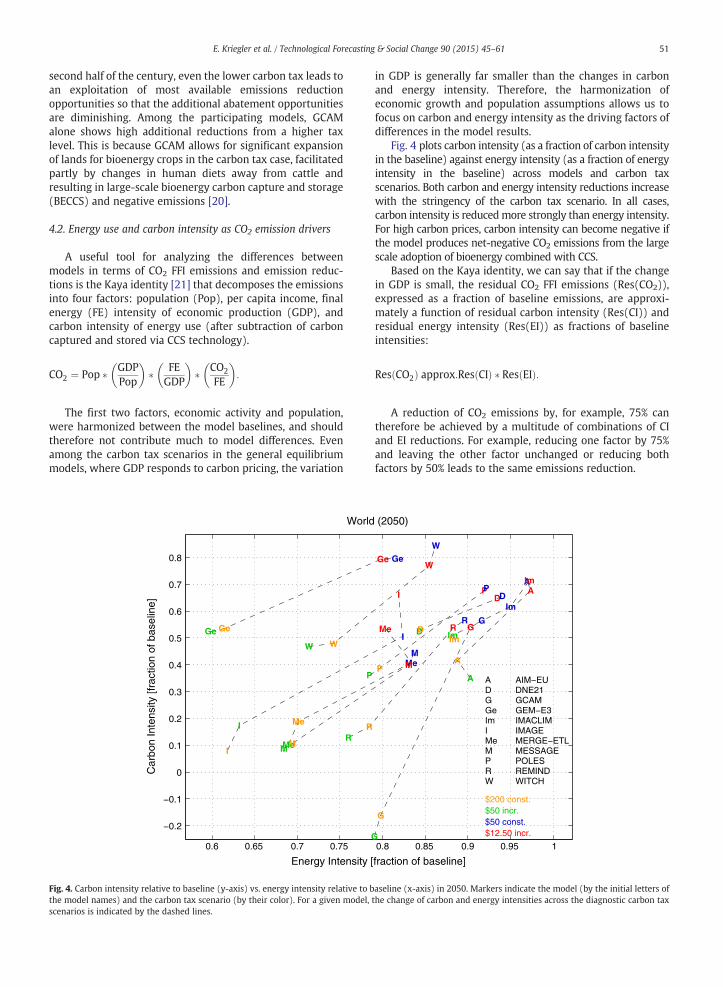
Fig. 4. Carbon intensity relative to baseline (y-axis) vs. energy intensity relative to bthe model names) and the carbon tax scenario (by their color). For a given model,scenarios is indicated by the dashed lines.

in GDP is generally far smaller than the changes in carbonand energy intensity. Therefore, the harmonization ofeconomic growth and population assumptions allows us tofocus on carbon and energy intensity as the driving factors ofdifferences in the model results.

Fig. 4 plots carbon intensity (as a fraction of carbon intensityin the baseline) against energy intensity (as a fraction of energyintensity in the baseline) across models and carbon taxscenarios. Both carbon and energy intensity reductions increasewith the stringency of the carbon tax scenario. In all cases,carbon intensity is reducedmore strongly than energy intensity.For high carbon prices, carbon intensity can become negative ifthe model produces net-negative CO2 emissions from the largescale adoption of bioenergy combined with CCS.

Based on the Kaya identity, we can say that if the changein GDP is small, the residual CO2 FFI emissions (Res(CO2)),expressed as a fraction of baseline emissions, are approxi-mately a function of residual carbon intensity (Res(CI)) andresidual energy intensity (Res(EI)) as fractions of baselineintensities:

Res CO2ð Þ approx:Res CIð Þ � Res EIð Þ:

A reduction of CO2 emissions by, for example, 75% cantherefore be achieved by a multitude of combinations of CIand EI reductions. For example, reducing one factor by 75%and leaving the other factor unchanged or reducing bothfactors by 50% leads to the same emissions reduction.

0.8 0.85 0.9 0.95 1

AA

A

A

DD

DD GG

G

Ge Ge

Im

Im

ImIm

I

IMe

MeMM

PP

P

RR

W

W

fraction of baseline]

(2050)

ADGGeImIMeMPRW

AIM−EUDNE21GCAMGEM−E3IMACLIMIMAGEMERGE−ETLMESSAGEPOLESREMINDWITCH

$12.50 incr.$50 const.$50 incr.$200 const.

aseline (x-axis) in 2050. Markers indicate the model (by the initial letters ofthe change of carbon and energy intensities across the diagnostic carbon tax


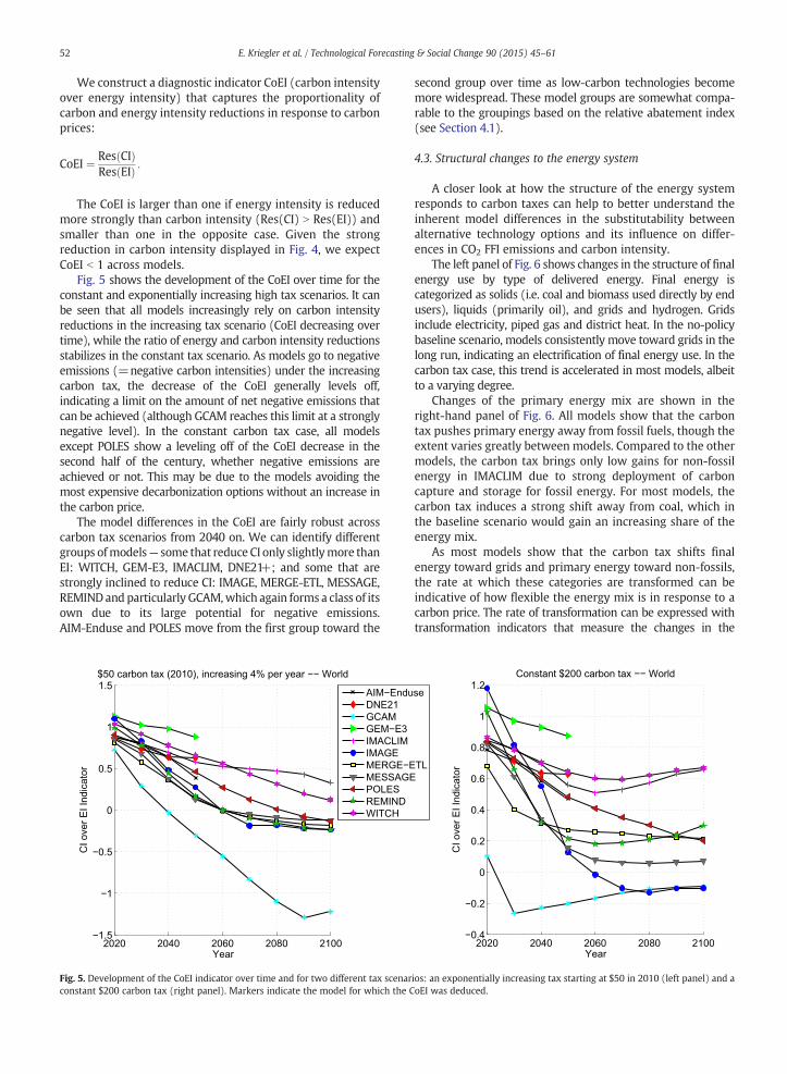
We construct a diagnostic indicator CoEI (carbon intensityover energy intensity) that captures the proportionality ofcarbon and energy intensity reductions in response to carbonprices:

CoEI ¼ Res CIð ÞRes EIð Þ :

The CoEI is larger than one if energy intensity is reducedmore strongly than carbon intensity (Res(CI) N Res(EI)) andsmaller than one in the opposite case. Given the strongreduction in carbon intensity displayed in Fig. 4, we expectCoEI b 1 across models.

Fig. 5 shows the development of the CoEI over time for theconstant and exponentially increasing high tax scenarios. It canbe seen that all models increasingly rely on carbon intensityreductions in the increasing tax scenario (CoEI decreasing overtime), while the ratio of energy and carbon intensity reductionsstabilizes in the constant tax scenario. As models go to negativeemissions (=negative carbon intensities) under the increasingcarbon tax, the decrease of the CoEI generally levels off,indicating a limit on the amount of net negative emissions thatcan be achieved (although GCAM reaches this limit at a stronglynegative level). In the constant carbon tax case, all modelsexcept POLES show a leveling off of the CoEI decrease in thesecond half of the century, whether negative emissions areachieved or not. This may be due to the models avoiding themost expensive decarbonization options without an increase inthe carbon price.

The model differences in the CoEI are fairly robust acrosscarbon tax scenarios from 2040 on. We can identify differentgroups ofmodels— some that reduce CI only slightlymore thanEI: WITCH, GEM-E3, IMACLIM, DNE21+; and some that arestrongly inclined to reduce CI: IMAGE, MERGE-ETL, MESSAGE,REMINDand particularly GCAM,which again forms a class of itsown due to its large potential for negative emissions.AIM-Enduse and POLES move from the first group toward the

Fig. 5. Development of the CoEI indicator over time and for two different tax scenarconstant $200 carbon tax (right panel). Markers indicate the model for which the C

second group over time as low-carbon technologies becomemore widespread. These model groups are somewhat compa-rable to the groupings based on the relative abatement index(see Section 4.1).

4.3. Structural changes to the energy system

A closer look at how the structure of the energy systemresponds to carbon taxes can help to better understand theinherent model differences in the substitutability betweenalternative technology options and its influence on differ-ences in CO2 FFI emissions and carbon intensity.

The left panel of Fig. 6 shows changes in the structure of finalenergy use by type of delivered energy. Final energy iscategorized as solids (i.e. coal and biomass used directly by endusers), liquids (primarily oil), and grids and hydrogen. Gridsinclude electricity, piped gas and district heat. In the no-policybaseline scenario, models consistently move toward grids in thelong run, indicating an electrification of final energy use. In thecarbon tax case, this trend is accelerated in most models, albeitto a varying degree.

Changes of the primary energy mix are shown in theright-hand panel of Fig. 6. All models show that the carbontax pushes primary energy away from fossil fuels, though theextent varies greatly between models. Compared to the othermodels, the carbon tax brings only low gains for non-fossilenergy in IMACLIM due to strong deployment of carboncapture and storage for fossil energy. For most models, thecarbon tax induces a strong shift away from coal, which inthe baseline scenario would gain an increasing share of theenergy mix.

As most models show that the carbon tax shifts finalenergy toward grids and primary energy toward non-fossils,the rate at which these categories are transformed can beindicative of how flexible the energy mix is in response to acarbon price. The rate of transformation can be expressed withtransformation indicators that measure the changes in the

ios: an exponentially increasing tax starting at $50 in 2010 (left panel) and aoEI was deduced.

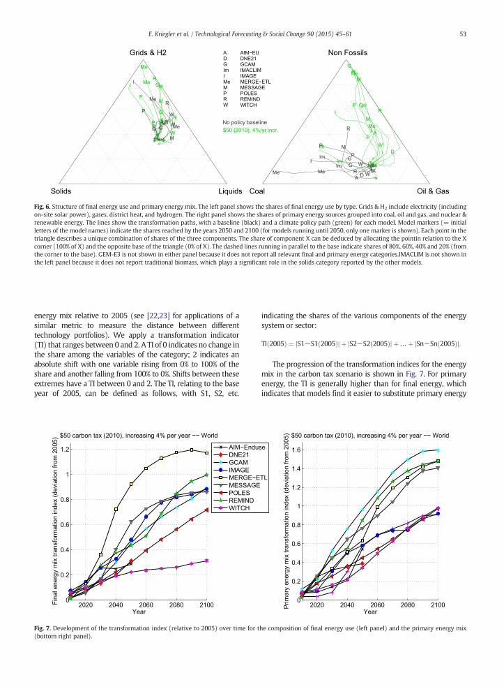
Fig. 6. Structure of final energy use and primary energy mix. The left panel shows the shares of final energy use by type. Grids & H2 include electricity (includingon-site solar power), gases, district heat, and hydrogen. The right panel shows the shares of primary energy sources grouped into coal, oil and gas, and nuclear &renewable energy. The lines show the transformation paths, with a baseline (black) and a climate policy path (green) for each model. Model markers (= initialletters of the model names) indicate the shares reached by the years 2050 and 2100 (for models running until 2050, only one marker is shown). Each point in thetriangle describes a unique combination of shares of the three components. The share of component X can be deduced by allocating the pointin relation to the Xcorner (100% of X) and the opposite base of the triangle (0% of X). The dashed lines running in parallel to the base indicate shares of 80%, 60%, 40% and 20% (fromthe corner to the base). GEM-E3 is not shown in either panel because it does not report all relevant final and primary energy categories.IMACLIM is not shown inthe left panel because it does not report traditional biomass, which plays a significant role in the solids category reported by the other models.


energy mix relative to 2005 (see [22,23] for applications of asimilar metric to measure the distance between differenttechnology portfolios). We apply a transformation indicator(TI) that ranges between 0 and 2. A TI of 0 indicates no change inthe share among the variables of the category; 2 indicates anabsolute shift with one variable rising from 0% to 100% of theshare and another falling from 100% to 0%. Shifts between theseextremes have a TI between 0 and 2. The TI, relating to the baseyear of 2005, can be defined as follows, with S1, S2, etc.

Fig. 7. Development of the transformation index (relative to 2005) over time for t(bottom right panel).

indicating the shares of the various components of the energysystem or sector:

TI 2005ð Þ ¼ S1−S1 2005ð Þj j þ S2−S2 2005ð Þj j þ…þ Sn−Sn 2005ð Þj j:

The progression of the transformation indices for the energymix in the carbon tax scenario is shown in Fig. 7. For primaryenergy, the TI is generally higher than for final energy, whichindicates that models find it easier to substitute primary energy

he composition of final energy use (left panel) and the primary energy mix


carriers and power generation types than to shift final energybetween solids, liquids and grids.

Somemodels show a clear correlation between the TIs forfinal energy and primary energy. GCAM, MERGE-ETL,MESSAGE and REMIND have a high TI for both final andprimary energy, whereas WITCH has a low TI for both andDNE21+ and POLES have medium values for both indices. Nosuch clear correlation can be seen for AIM-Enduse andIMAGE. AIM-Enduse starts with a low primary energy TI thatshows an upward trend after 2040 – partly due to increasingmarket maturity of solar power – while its final energy TIremains low. IMAGE has medium primary energy TI, but itsfinal energy TI is high indicating that IMAGE relies more onsubstitution of energy end use carriers than other models.

4.4. Economic implications of carbon pricing

4.4.1. Mitigation costsThe economic implications of a carbon tax are typically

captured in terms of mitigation costs that are derived fromcomparing the policy scenario with the counterfactualbaseline case that does not include climate policy. For generalequilibrium models, the mitigation costs can be expressed aslosses in welfare, consumption or GDP relative to the baselinecase. The first two metrics directly measure the impact onprivate income and consumption. GDP is a less satisfactoryindicator because it is a measure of output, which includesnot only consumption, but also investment, imports, exports,and government spending [24]. Partial equilibrium models donot include the feedback on economy-wide production andhousehold consumption but can express mitigation costs interms of the change in consumer and producer surplus oftendeduced from the area under the marginal abatement costcurve. An alternative measure is additional energy systemcosts compared to the baseline case.

Fig. 8. Intertemporally aggregated mitigation costs (as a percentage of baseline con(right column). Cost measures differ for general (to the right of the vertical line) abottom in the figure legend are shown from left to right bars for each model.

The mitigation costs from general and partial equilibriummodels are not fully comparable. We nonetheless present costsfrombothmodel types next to each other, especially focusing onthe relative changes. Comparisons between the cost measuresshown by GEs and PEs have shown that in relative terms, theyseem to correlate reasonably well across scenarios and regions[25]. The intertemporally aggregated mitigation costs from thegeneral equilibrium models in this diagnostics study (GEM-E3,IMACLIM, MERGE-ETL, MESSAGE, REMIND,WITCH) are given interms of the net present value of consumption losses as apercentage of net present value consumption in the baseline (alldiscounted at 4% per year). The intertemporal mitigation costsfrom the partial equilibrium models (DNE21+, GCAM, IMAGE,POLES) are given in terms of the net present value of the areaunder the MAC curve (GCAM, IMAGE, POLES) or in terms ofadditional energy system costs (DNE21+) as a percentage of netpresent valueGDP in the baseline (all discounted at 4% per year).

Fig. 8 shows the aggregate global mitigation costs for theperiods 2010–2050 and 2010–2100 across carbon taxscenarios. All models show an increase in mitigationcosts until 2050 with the stringency of carbon taxes ($12.50increasing b $50 constant b $50 increasing b $200 constant).The picture for 2010–2100 is mixed. Both the low constant andthe low increasing tax scenarios come in at similar costs ($50constant, $12.50 increasing), as do the high constant and highincreasing tax scenarios ($200 constant, $50 increasing).Although the carbon price in the increasing tax scenario risesfar higher over the second half of the century, the constant taxscenario includes the impact of an early price shock. Modelsdiffer onwhich tax scenario leads to the highest costs until 2100.With the exception of GCAM, the partial equilibrium modelsshow lower mitigation costs than the general equilibriummodels. This is an indication of the differences in cost metrics.GCAM is an exception that may be explained by the very highabatement response to carbon pricing shown by this model.

sumption or GDP) for the periods 2010–2050 (left column) and 2010–2100nd partial equilibrium models (to the left). The scenarios listed from top to

Fig. 9. Intertemporally aggregated mitigation costs (y-axis) are plotted against cumulated CO2 FFI emissions reductions (fraction of baseline; x-axis). Results for2050 are shown separately for general equilibrium models (left panel) and for partial equilibrium models (right panel). The dashed lines connect data pointsacross carbon tax scenarios (shown by marker color) for a given model (shown by the initials of the model names as markers).


Among all models, IMACLIM stands out by showing the highestmitigation costs across scenarios. This is due to assumptions ofimperfect foresight combined with market and institutionalimperfections that, under a carbon tax, can result in GDP lossesthat are far more significant than in the case of economies withfrictionless markets and non-distortive fiscal systems.

Fig. 9 shows a positive correlation between mitigationcosts and cumulative emissions reductions from differentcarbon tax scenarios in 2050. This correlation is still mostlyintact in 2100, although somemodels (IMACLIM, MESSAGE,WITCH) suggest that the increasing high tax case ($50increasing) can lead to somewhat lower cost relative to theamount of emission reductions than the constant high ($200)tax case. The initial shock from the constant $200 tax can bevery costly in the short term, and the 4% discount rate gives alarge weight to such short-term losses.

4.4.2. Cost per abatement valueAs can be seen in Figs. 8 and 9, differences in the cost levels

across models increase with increasing mitigation costs in themore stringent carbon tax scenarios. We can study the modeldifferences through a cost per abatement value (CAV) indicatortaking into account the mitigation costs (MitCosts) over theperiod from 2010 to year t, discounted at a rate r of 4% per yearrelative to the value of reduced emissions, measured ingreenhouse gas emissions reduction (GHG Red) times thecarbon price (CPrice) over the same period 2010 to t, alsodiscounted at 4%. This measure includes all Kyoto gasesrepresented in a model since the study setup assumes thatthe carbon tax is applied to Kyoto gases aside fromCO2 by usingglobal warming potentials (GWPs) as conversion factors. TheCAV is defined as follows:

CAV Tð Þ ¼XT

2010MitCosts tð Þ � 1þ rð Þ2010−t

XT2010

GHG Red tð Þ � CPrice tð Þ � 1þ rð Þ2010−t :

The result is a dimensionless number signifying theeconomic implications of emissions abatement resultingfrom carbon pricing. A high CAV means comparativelyhigher mitigation costs for a given emissions reduction andcarbon price trajectory than in the case with a low CAV. Forpartial equilibrium models, it essentially describes the ratiobetween average and marginal abatement costs. For generalequilibrium models, macro-economic feedbacks are alsofactored in. This becomes particularly evident for IMACLIM,for which the CAV exceeds unity until mid-century.

Fig. 10 shows the development of the cost per abatementvalue indicator for the exponentially increasing and constanthigh tax scenarios. In the exponential carbon tax case, theCAV is declining over time for all models. This indicates thatafter discounting, the increase in mitigation cost is morethan outweighed by the increase in emission reductions,taking into account that the present value of the carbon taxremains constant when assuming a discount rate of 4% peryear. The constant tax scenario results in a relativelyconstant CAV.

The ordering of models in terms of CAV is largely preservedover time and across the increasing and constant tax scenarios.IMACLIM shows CAV values that are multiple times as high asthose of the other models. DNE21+, GEM-E3, GCAM, REMINDand WITCH have medium CAV values. IMAGE, MERGE-ETL,MESSAGE, and POLES come in at the low end.

5. Model characterization based on diagnostic indicators

We have developed a set of diagnostic indicators tocharacterize the model response to carbon pricing in variousdimensions:

• Cumulated CO2 FFI emissions reductions (relative abatementindex)

• Carbon intensity vs. energy intensity reductions (CoEI indicator)

Fig. 10. Development of the cost per abatement value (CAV) indicator over time and for two different tax scenarios: an exponentially increasing tax starting at $50in 2010 (left panel) and a constant $200 carbon tax (right panel). Markers indicate the model for which the CAV was deduced. Solid lines indicate GE models,whereas dotted lines indicate PE models.


• Structural changes in energy use (primary energy transforma-tion index)4

• Mitigation costs (cost per abatement value).

In Section 5.1, we check for correlations among theseindicators to examine the potential to classify models basedon indicator combinations. Section 5.2 presents a preliminarymodel classification scheme.

5.1. Correlation of indicators

A large response of the primary energy mix to a carbontax will result in a strong reduction of carbon intensity as, inmost models, the primary energy mix shifts away from fossilfuels due to the tax. We would thus expect that models witha high primary energy TI are strongly inclined to reducecarbon intensity and exhibit a relatively low carbon overenergy intensity (CoEI) values. Everything else being equal, alower carbon intensity translates to lower emissions andthus higher emissions abatement. Fig. 11 plots the primaryenergy TI results of this study against the CoEI. Fig. 12 plotsthe primary energy TI against the relative abatement index(RAI). While a negative correlation between the TI and theCoEI and a positive correlation between the TI and the RAIare clearly confirmed, these correlations are stronger in2050 than in 2100. This is because even a strong transfor-mation of the primary energymix toward low carbon energysources reaches its limits in further reducing carbonintensity and emissions — except in GCAM, where the large

4 We use the transformation index for primary energy supply to representthe structural changes in the energy system since it shows the moresignificant changes among the transformation indices discussed in Sec-tion 4.3 and is also the most broadly applicable to existing modelingframeworks.

shift to bioenergy with CCS continues to boost negativeemissions as carbon prices increase.

We also investigate the correlation of the CoEI with theRAI (Fig. 13). There is indeed a negative correlation betweenCoEI and RAI. Higher relative abatement (high RAI) tends tocome with a strong inclination to reduce CI (low CoEI). Thenegative correlation of RAI and CoEI is strongest in situationsof a significant carbon tax signal that has not yet pushed thedecarbonization to its limits. In the case of a low carbon taxsignal, the model response may not be strong enough toinduce a clear correlation (see Fig. S2 in the SOM).

The correlation between the abatement response tocarbon prices and the inclination to reduce carbon intensityis an important result of our diagnostic analysis. The RAI andCoEI are complementary by construction, since the RAI isrelated to the residual CO2 FFI emissions, which in principlecan be achieved with a large range of CoEIs. The negativecorrelation between the RAI and CoEI (Fig. 13), the positivecorrelation between the RAI and the TI (Fig. 12), and thenegative correlation between the TI and CoEI (Fig. 11)suggest that many models show a high/low/high or a low/high/low pattern for RAI/CoEI/TI.

5.2. Model classification

Section 5.1 has identified correlations among the diag-nostic indicators on emissions, energy and carbon intensity,and energy system response. This means that their combi-nationmight allow us to characterize not only a single modelbut also a larger group of models. Such a classification wouldmake it easier to identify patterns among the spread ofmodel results in model intercomparison studies that aim toinform policy-relevant questions. What follows is only apreliminary attempt at such a classification that aims toillustrate one important application of model diagnostics.

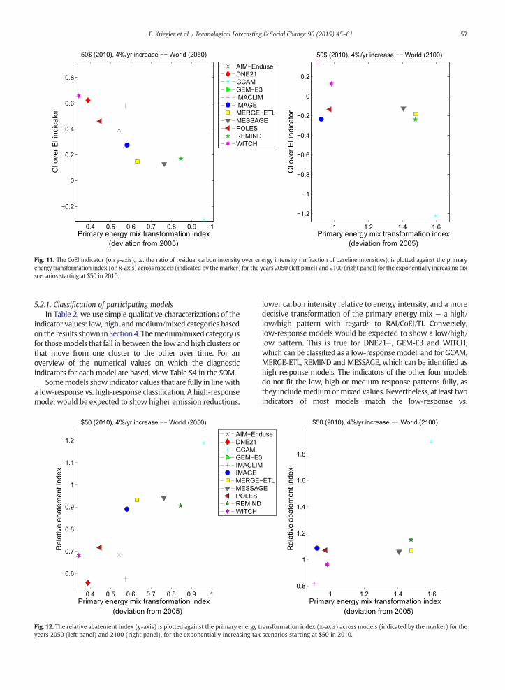
Fig. 11. The CoEI indicator (on y-axis), i.e. the ratio of residual carbon intensity over energy intensity (in fraction of baseline intensities), is plotted against the primaryenergy transformation index (on x-axis) acrossmodels (indicated by themarker) for the years 2050 (left panel) and 2100 (right panel) for the exponentially increasing taxscenarios starting at $50 in 2010.


5.2.1. Classification of participating modelsIn Table 2, we use simple qualitative characterizations of the

indicator values: low, high, andmedium/mixed categories basedon the results shown in Section4. Themedium/mixed category isfor thosemodels that fall in between the low and high clusters orthat move from one cluster to the other over time. For anoverview of the numerical values on which the diagnosticindicators for each model are based, view Table S4 in the SOM.

Somemodels show indicator values that are fully in linewitha low-response vs. high-response classification. A high-responsemodel would be expected to show higher emission reductions,

Fig. 12. The relative abatement index (y-axis) is plotted against the primary energy tyears 2050 (left panel) and 2100 (right panel), for the exponentially increasing tax

lower carbon intensity relative to energy intensity, and a moredecisive transformation of the primary energy mix — a high/low/high pattern with regards to RAI/CoEI/TI. Conversely,low-response models would be expected to show a low/high/low pattern. This is true for DNE21+, GEM-E3 and WITCH,which can be classified as a low-response model, and for GCAM,MERGE-ETL, REMIND and MESSAGE, which can be identified ashigh-response models. The indicators of the other four modelsdo not fit the low, high or medium response patterns fully, asthey includemedium ormixed values. Nevertheless, at least twoindicators of most models match the low-response vs.

ransformation index (x-axis) across models (indicated by the marker) for thescenarios starting at $50 in 2010.

Fig. 13. The CoEI indicator (y-axis) is plotted over the relative abatement index (x-axis) across models (indicated by the marker) for the years 2050 (left panel)and 2100 (right panel) for the exponentially increasing tax scenarios starting at $50 in 2010.


high-response patterns. For this preliminary classification, wedefine IMACLIM as a low-response model, IMAGE as ahigh-response model and AIM-Enduse and POLES asmedium-response models based on the largest overlap withthe low/medium/high response classes defined in Table 3.

There is no clear correlation between the cost perabatement value (CAV) indicator and the model classifica-tion based on RAI, CoEI and TI. This may be due to the factthat high-response models may exhibit both relatively highemission reductions and high mitigation costs that boostboth the numerator and the denominator of the CAV. Thiswould indicate that the CAV provides complementaryinformation to the high- vs. low-response model character-istics. Section 4.4 suggests that high CAV values come fromthe subset of equilibriummodels that include the full impacton the economy.

It is worthwhile noting that some of themodels classifiedas low response models in Table 2 are also among themodels with a low measure of low-carbon energy supplytechnology variety, as shown in Table 1. However, a hightechnology variety measure does not automatically lead to

Table 2Qualitative description of indicator values across individual models and diagnostic iavailable to calculate the particular indicator. A preliminary classification of modecolumn.

Model Relative abatement index CoEI indicator Transformation inde

AIM-Enduse Low Mixed MixedDNE21+ Low High LowGCAM High Low HighGEM-E3 Low High TBDIMACLIM Low High MixedIMAGE High Low MixedMERGE-ETL High Low HighMESSAGE High Low HighPOLES Mixed Mixed LowREMIND High Low HighWITCH Low High Low

the classification as a high-response model. The measureonly covers the supply side, and a high variety of low-carbontechnologies does not automatically translate into theirlarge-scale use.

5.2.2. Preliminary classification schemeFrom our classification of the participating models, we

derive a preliminary classification scheme based on theindicators RAI, CoEI and TI and the model type (Table 3).

We have added the model type to the classificationscheme rather than the CAV itself because the model typedetermines the cost components that can actually bemeasured. However, this may be changed in the future, orthe CAV may be added, as our understanding about theexplanatory power of the CAV improves. The CAV definitelyprovides useful additional information about the magnitudeof mitigation costs in climate policy analyses with quantita-tive mitigation targets. In such a setting, the requiredemissions reductions are largely fixed, and the low vs. highresponsiveness of models will give a good indication aboutthe level of carbon prices that is needed in the models to

ndicators. TBD (To be defined) is shown in places where model data was notls based on the combination of indicator values is shown in the rightmost

x (primary energy) Cost per abatement value Classification

TBD PE — medium responseMixed PE — low responseMedium PE — high responseMedium GE — low responseHigh GE — low responseLow PE — high responseLow GE — high responseLow GE — high responseLow PE — medium responseMedium GE — high responseMedium GE — low response

Table 3Criteria for a preliminary classification of models based on qualitativedescriptions of indicator values.

Modeltype

Modelclassification

Relativeabatementindex

CoEIindicator

Transformationindex (primaryenergy)

PE/GE Low response Low High LowPE/GE Medium

responseMedium/Mixed

Medium/Mixed

Medium/Mixed

PE/GE High response High Low High


reach the target. Thus, the choice of mitigation target and theresponsiveness of models largely determine the denomina-tor of the CAV. The indicator itself will then specify to whatextent the abatement value translates into mitigation costs.Therefore, highest cost estimates can be expected fromgeneral equilibrium models measuring full economic costswith low responsiveness and high CAV (IMACLIM and to alesser extent GEM-E3 and WITCH). In turn, lowest costestimates will be expected in partial equilibrium modelswith high responsiveness and low CAV (IMAGE).

We note that models that do not match but are close tothe indicator patterns in Table 3 can also be classified basedon this scheme. For instance, a model with a low abatementindex, a high CoEI and a medium or mixed transformationindex can be considered a low-response model.

The derived preliminary classification serves mainlyillustrative purposes. Further research and the integrationof diagnostic results from more models are needed toestablish a robust classification scheme. Ultimately, thevalue of such a scheme needs to be judged against its abilityto characterize differences in model outputs and policyimplications in a variety of contexts. As a preliminary testof the model classification, we present results from the

Fig. 14.Mitigation costs plotted against cumulated CO2 FFI emissions reductions (frascenarios (connected by dashed lines for a given model). Models are colored accorresponse: Dark Red; PE— high response: Green; GE— low response: Black; GE— higof most models' graphs, these panels exclude IMACLIM, which shows NPV policy cothe periods 2010–2050 and 2010–2100.

AMPERE model intercomparison studies on delayed andfragmented action [6,7] in Fig. 14. These results are fromscenarios for atmospheric greenhouse gas concentrationtargets at levels of approx. 450 and 550 ppm CO2e. Fig. 14shows mitigation costs (in NPV consumption or partialequilibrium costs, discounted at 4% per year) for the 450 and550 ppm CO2eq stabilization cases. Models are coloredaccording to the classification identified above. It canbe seen that costs decrease from low-response to high-response models and are higher for GE than for PE models.As expected, IMACLIM exhibits the highest costs (exceedingthe upper boundaries of Fig. 14) and IMAGE the lowest. Thus,our preliminary classification passes this initial test of itsexplanatory power for the differences in cost estimates.However, the test sample is too small to draw definitiveconclusions at this point.

It should finally be noted that the classification that we usedhere relates to specific versions of the respective models.Updates in model structure or parameters could change therelative position of different models, for instance through theinclusion of new mitigation options.

6. Summary and conclusion

We have studied and compared the emissions, energy,and economic response to a carbon price signal across 11global energy-economy and integrated assessment models.The diagnostic study setup consisted of a no-climate-policybaseline and a series of constant and exponentially risingcarbon tax scenarios with globally harmonized carbon prices.The study setup can be adopted by global and regionalmodels alike. We found the increasing tax variant to be mostuseful for identifying diagnostic indicators for abatementresponse and economic impacts because the present value of

ction of baseline emissions) for 450 and 550 ppm CO2eq climate stabilizationding to the classification in Table 3 (PE — low response: Red, PE — mediumh response: Yellow). To keep the y-axis at a scale that provides good visibilitysts of 6–7% for the 550 ppm scenario and 9–10% for the 450 ppm scenario for


a constant carbon tax depreciates over time in the dynamicsetting of a growing economy.

We have developed four diagnostic indicators to charac-terize the model responses based on the criteria of charac-terizing model heterogeneity, relevance for climate policyanalysis, applicability to diverse models, and accessibility andease of use. These indicators are the relative abatement index(RAI), measuring the scale of emissions reductions, thecarbon over energy intensity indicator (CoEI) measuring thereliance on carbon intensity vs. energy intensity reductions,the transformation index (TI) measuring the scale of trans-forming the primary energy mix, and the cost per abatementvalue (CAV) indicator measuring the mitigation costs as afunction of carbon prices and emissions reductions.

A key result of the diagnostic analysis is the identification ofstrong correlations between the different diagnostic indicators.Models with higher relative abatement (high RAI) tend to alsoexhibit a stronger reliance on carbon intensity reductions (lowCoEI) and amore significant transformation of the energy sector(high transformation indices). At the opposite end, we findmodels with lower relative abatement, a smaller reliance oncarbon intensity reductions (high CoEI) and much smallerchanges to the structure of the energy system (low transforma-tion indices). When compared with each other, most modelsthat participated in the diagnostic study fell into one of these twocategories. These correlations point to a distinct fingerprint ofmodel structure that emerges in various dimensions.

We used the correlation between diagnostic indicators toestablish a preliminary classification scheme and to illustratepotential next steps in the diagnostic work. Establishing andvetting a robust and useful classification scheme will requirea community effort involving more models and diagnosticexperiments as well as tests in applied contexts. We arehopeful that the findings and suggestions presented here canhelp encourage the next research steps and advance thediscussion about diagnostic standards.

Acknowledgment

The research leading to these results has received fundingfrom the European Union's Seventh Framework ProgrammeFP7/2010 under grant agreement n° 265139 (AMPERE).Aurélie Méjean also acknowledges funding from the Chair"Modeling for Sustainable Development" led by ParisTech.

Appendix A. Supplementary data

Supplementary data to this article can be found online athttp://dx.doi.org/10.1016/j.techfore.2013.09.020.

References

[1] J.P. Weyant, F.C. de la Chesnaye, G.J. Blanford, Overview of EMF-21:Multigas Mitigation and Climate Policy. Energy J. 27 (Special Issue 3)(2006) 1–32.

[2] L. Clarke, J. Edmonds, V. Krey, R. Richels, S. Rose, M. Tavoni,International climate policy architectures: overview of the EMF 22international scenarios, Energy Econ. 31 (2) (2009) S64–S81.

[3] O. Edenhofer, B. Knopf, M. Leimbach, N. Bauer, The economics of lowstabilization, Energy J. 31 (Special Issue I) (2010).

[4] G. Luderer, V. Bosetti, M. Jakob, M. Leimbach, J. Steckel, H. Waisman, O.Edenhofer, On the economics of decarbonization — results and insightsfrom the RECIPE project, Clim. Chang. 114 (1) (2012) 9–37.

[5] J.P. Weyant, O. Davidson, H. Dowlatabadi, J. Edmonds, M. Grubb, E.A.Parson, R. Richels, J. Rotmans, P.R. Shukla, R.S.J. Tol, Integratedassessment of climate change: an overview and comparison ofapproaches and results, in: J.P. Bruce, H. Lee, E.F. Haites (Eds.),Climate Change 1995: Economic and Social Dimensions ofClimate Change, Cambridge University Press, Cambridge, UK, 1996,pp. 367–439.

[6] E. Kriegler, K. Riahi, N. Bauer, V.J. Schwanitz, N. Petermann, V. Bosetti, A.Marcucci, S. Otto, L. Paroussos, S. Rao, T.A. Currás, S. Ashina, J. Bollen, J.Eom, M. Hamdi-Cherif, T. Longden, A. Kitous, A. Méjean, F. Sano, M.Schaeffer, K. Wada, P. Capros, D.P. van Vuuren, O. Edenhofer, Making orbreaking climate targets the AMPERE study on staged accession scenariosfor climate policy, Technol. Forecast. Soc. Chang. 90 (2015) 24–44 (in thisissue).

[7] K. Riahi, E. Kriegler, N. Johnson, C. Bertram, M. den Elzen, J. Eom, M.Schaeffer, J. Edmonds, M. Isaac, V. Krey, T. Longden, G. Luderer, A.Méjean, D.L. McCollum, S. Mima, H. Turton, D.P. Van Vuuren, K.Wada, V. Bosetti, P. Capros, P. Criqui, M. Hemdi-Cherif, M. Kainuma,O. Edenhofer, Locked into Copenhagen pledges — implications ofshort-term emission targets for the cost and feasibility of long-termclimate goals, Technol. Forecast. Soc. Chang. 90 (2015) 8–23 (in thisissue).

[8] J.P. Weyant, A perspective on integrated assessment, Clim. Change 95(2009) 317–323.

[9] W.M. Washington, G.A. Meehl, General circulation model experiments onthe climatic effects due to a doubling and quadrupling of carbon dioxideconcentration, J. Geophys. Res. 88 (C11) (1983) 6600–6610.

[10] D.W. Gaskins, J.P. Weyant, Model comparisons of the costs of reducingCO2 emissions, Am. Econ. Rev. 83 (2) (1993) 318–323.

[11] K. Calvin, L. Clarke, V. Krey, G. Blanford, K. Jiang, M. Kainuma, E.Kriegler, G. Luderer, P.R. Shukla, The role of Asia in mitigating climatechange: results from the Asia modeling exercise, Energy Econ. 34 (3)(2012) S251–S260.

[12] J.P. Weyant, EMF-19 alternative technology strategies for climatechange policy, Energy Econ. 26 (4) (2004) 501–755.

[13] D.P van Vuuren, M. Hoogwijk, T. Barker, K. Riahi, S. Boeters, J. Chateau,S. Scrieciu, J. van Vliet, T. Masui, K. Blok, E. Blomen, T. Kram,Comparison of top-down and bottom-up estimates of sectoral andregional greenhouse gas emission reduction potentials, Energy Policy37 (2009) 5125–5139.

[14] J. Weyant, Program on Integrated Assessment Model Development,Diagnostics and Inter-Model Comparison (PIAMDDI): an overview,IAMC Annual Meeting, 2010, (http://www.globalchange.umd.edu/iamc_data/iamc2010/PIAMDDI_Overview.pdf, last accessed September2013).

[15] Integrated Assessment Modeling Consortium, IIASA, 2012. (http://www.globalchange.umd.edu/iamc, last accessed September 2013).

[16] J.C. Hourcade, M. Jaccard, C. Bataille, F. Ghersi, Hybrid modeling: newanswers to old challenges, the energy journal, Energy J. 27 (SpecialIssue 2) (2006) 1–12.

[17] T. Hanaoka, M. Kainuma, Low-carbon transitions in world regions:comparison of technological mitigation potential and costs in 2020and 2030 through bottom-up analyses, Sustain. Sci. 7 (2) (2012)117–137.

[18] K. Conrad, Computable general equilibrium models in environmentaland resource economics, in: T. Tietenberg, H. Folmer (Eds.), TheInternational Yearbook of Environmental and Resource Economics2002/03, Edward Elgar, Cheltenham, UK, 2002.

[19] G.J. Blanford, E. Kriegler, M. Tavoni, Harmonization vs. Fragmentation:overview of climate policy scenarios in EMF27, Clim. Chang. (2014),http://dx.doi.org/10.1007/s10584-013-0951-9(online first).

[20] M. Wise, K. Calvin, A. Thomson, L. Clarke, B. Bond-Lamberty, R. Sands,et al., Implications of limiting CO2 concentrations for land use andenergy, Science 324 (5931) (2009) 1183–1186.

[21] Y. Kaya, K. Yokobory, Environment, Energy, and Economy: Strate-gies for Sustainability, United Nations University Press, Tokyo,Japan, 1998.

[22] L. Clarke, V. Krey, J. Weyant, V. Chaturvedi, Regional energy systemvariation in global models: results from the Asian modeling exercisescenarios, Energy Econ. 34 (3) (2012) S293–S305.

[23] V. Krey, K. Riahi, Risk hedging strategies under energy system andclimate policy uncertainties, IIASA Interim Report IR-09-028,International Institute for Applied Systems Analysis, Laxenburg,Austria, 2009.

[24] S. Paltsev, P. Capros, Cost Concepts for Climate Change Mitigation,Climate Change Economics 4 (supp01) (2013)1340003.

[25] A.F. Hof, M.G.J. den Elzen, D.P. van Vuuren, Environmental effectivenessand economic consequences of fragmented versus universal regimes:what can we learn from model studies? Int. Environ. Agreements 9(2009) 39–62.


http://refhub.elsevier.com/S0040-1625(13)00257-6/rf0005




















































http://www.globalchange.umd.edu/iamc_data/iamc2010/PIAMDDI_Overview.pdf

http://www.globalchange.umd.edu/iamc_data/iamc2010/PIAMDDI_Overview.pdf

http://www.globalchange.umd.edu/iamc

http://www.globalchange.umd.edu/iamc












http://dx.doi.org/10.1007/s10584-013-0951-9






















Elmar Kriegler is deputy chair of the Research Domain Sustainable Solutionsat the Potsdam Institute for Climate Impact Research (PIK), Germany. Hisprincipal research focuses on the integrated assessment of climate changeand scenario development.

Nils Petermann is a project coordinator at the Potsdam Institute for ClimateImpact Research. His focus is the EU project AMPERE, dedicated to modelanalysis of climate change mitigation pathways.

Volker Krey is the deputy program leader of the Energy Program at theInternational Institute for Applied Systems Analysis (IIASA), Austria. Hisscientific interests focus on the integrated assessment of climate change andthe energy challenges.

Valeria Jana Schwanitz is a post-doctoral researcher at the PostdamInstitute of Climate Impact Research. She is a member of the Global EnergySystems and Macroeconomic Modeling research groups.

Gunnar Luderer is a senior researcher at the Potsdam Institute for ClimateImpact Research. He is head of the Global Energy Systems group at PIK.

Shuichi Ashina is a researcher focusing on energy-economy-environmentalsystems modeling at the Center for Social and Environmental Systems Researchof the National Institute for Environmental Studies (NIES), Japan.

Valentina Bosetti is climate change topic leader and a modeler for theSustainable Development Programme at FEEM, Italy. Since 2012, she is also anassociate professor at the Department of Economics, Bocconi University.

Jiyong Eom is a staff scientist at the Pacific Northwest National Laboratory'sJoint Global Change Research Institute, USA. His principal research focuseson integrated assessment of global environmental problems.

Alban Kitous is Scientific Officer at the European Commission Joint ResearchCenter. He is a specialist in energy economic modeling and policy assessment.

Aurélie Méjean is a research fellow at the International Research Centre onEnvironment and Development (CIRED, France). She is a member of theenergy-economy-environment modeling team.

Leonidas Paroussos is a senior researcher at the E3M-Lab/ICCS and he isexperienced in climate change policy assessment using general equilibriummodels, environmental economics and energy analysis.

Fuminori Sano is a research scientist at the Research Institute of InnovativeTechnology for the Earth (RITE). His research focuses on the assessment ofclimate change mitigation technologies and policies.

Hal Turton leads the Energy Economics Group at the Paul Scherrer Institute(PSI). His research focuses on scenario analysis of global and Europeanenergy system development, integration of energy and economic models,and technology assessment.

Charlie Wilson is a lecturer in energy and climate change research at theUniversity of East Anglia, UK. His research interests lie at the intersectionbetween innovation, behavior and policy in the field of energy and climatechange mitigation.

Detlef P. van Vuuren is a senior researcher at PBL Netherlands Environ-mental Assessment Agency — working on integrated assessment of globalenvironmental problems. He is also a professor at the Copernicus Institutefor Sustainable Development at Utrecht University.

Diagnostic indicators for integrated assessment models of ...

Documents

Transcript of Diagnostic indicators for integrated assessment models of ...