Structural Agnostic Modeling: Adversarial Learning ofCausal Graphs

Diviyan Kalainathan∗ DIVIYAN@FENTECH.AIFentech20 Rue Raymond Aron, Paris, France

Olivier Goudet∗ OLIVIER.GOUDET@UNIV-ANGERS.FRLERIA, Universite d’Angers2 boulevard Lavoisier, 49045 Angers, France

Isabelle Guyon GUYON@CHALEARN.ORGTAU, LRI, INRIA, CNRS, Universite Paris-Saclay660 Rue Noetzlin, Gif-Sur-Yvette, France

David Lopez-Paz DLP@FB.COMFacebook AI Research6 Rue Menars, 75002 Paris

Michele Sebag SEBAG@LRI.FR

TAU, LRI, INRIA, CNRS, Universite Paris-Saclay660 Rue Noetzlin, Gif-Sur-Yvette, France

Editor:

AbstractA new causal discovery method, Structural Agnostic Modeling (SAM), is presented in this paper.Leveraging both conditional independencies and distributional asymmetries in the data, SAM aimsto find the underlying causal structure from observational data. The approach is based on a gamebetween different players estimating each variable distribution conditionally to the others as a neuralnet, and an adversary aimed at discriminating the overall joint conditional distribution, and that ofthe original data. A learning criterion combining distribution estimation, sparsity and acyclicityconstraints is used to enforce the end-to-end optimization of the graph structure and parametersthrough stochastic gradient descent. Besides a theoretical analysis of the approach in the largesample limit, SAM is extensively experimentally validated on synthetic and real data.

1. Introduction

This paper addresses the problem of uncovering causal structure from multivariate observationaldata. This problem is receiving more and more attention with the increasing emphasis on modelinterpretability and fairness (Doshi-Velez and Kim, 2017). While the gold standard to establish causalrelationships remains randomized controlled experiments (Pearl, 2003; Imbens and Rubin, 2015), inpractice these often happen to be costly, unethical, or simply infeasible. Therefore, hypothesizingcausal relations from observational data, often referred to as observational causal discovery, hasattracted much attention from the machine learning community (Lopez-Paz et al., 2015; Mooij

.∗ Equal contribution. This work was done during Olivier Goudet’s post-doc at Univ. Paris-Saclay and Diviyan Kalainathan’s PhD atUniv. Paris-Saclay.

1

arX

iv:1

803.

0492

9v4

[st

at.M

L]

20

Sep

2021

et al., 2016; Peters et al., 2017). Observational causal discovery has found many applications, e.g.in economics to understand and model the impact of monetary policies (Chen et al., 2007), orin bio-informatics to infer network structures from gene expression data (Sachs et al., 2005) andprioritize confirmatory or exploratory experiments.

Observational causal discovery aims to learn the causal graph from samples of the joint probabilitydistribution of observational data. Four main approaches have been proposed in the literature (morein Section 2.4).

A first approach refers to score based methods, using local search operators to navigate in thespace of Directed Acyclic Graphs (DAGs) in order to find the Markov equivalence class of the graphoptimizing the considered score (Chickering, 2002; Ramsey, 2015). A second approach includesconstraint-based methods leveraging conditional independence tests to identify the skeleton of thegraph and the v-structures (Spirtes et al., 1993; Colombo et al., 2012). A third approach embodieshybrid algorithms, combining ideas from constraint-based and score-based algorithms (Tsamardinoset al., 2006; Ogarrio et al., 2016). The fourth approach goes beyond the Markov equivalence classlimitations by exploiting asymmetries in the joint distribution, e.g. based on the assumption thatp(x)p(y|x) is simpler than p(y)p(x|y) (for some appropriate notion of simplicity) when X causesY (Hoyer et al., 2009; Zhang and Hyvarinen, 2010; Mooij et al., 2010). Another stream of workclosely related to causal discovery is the causal feature selection, aiming at recovering the MarkovBlanket of target variables (Yu et al., 2018). It leverages the estimation of mutual information amongvariables (Bell and Wang, 2000; Brown et al., 2012; Vergara and Estevez, 2014) or uses classificationor regression models to support variable selection (Aliferis et al., 2003, 2010).

The contribution of this paper is a new causal discovery algorithm called Structural AgnosticModeling (SAM),1 restricted to continuous variables, which aims to exploit both conditional inde-pendence relations and distributional asymmetries from observational data. SAM searches for anacyclic Functional Causal Model (FCM) (Pearl, 2003) with neural networks that aim to model thecausal mechanisms while achieving an optimal complexity/fit trade-off.

SAM proceeds as follows: i) each causal mechanism in the FCM is a neural net trained fromavailable data; ii) the combinatorial optimization problem, at the root of directed acyclic graphlearning, is handled through sparsity and acyclicity constraints inspired from Leray and Gallinari(1999) and Yu et al. (2018); iii) the joint training of all causal mechanisms is handled in parallel onGPU devices through an adversarial approach (Goodfellow et al., 2014; Mirza and Osindero, 2014),enforcing the accuracy of the FCM joint distribution with respect to the data distribution. SAM alsorelies on Occam’s razor principle to infer the causal graph, where the complexity of each candidategraph is evaluated as an aggregation of structural and functional complexity scores.

This paper is organized as follows: Section 2 introduces the problem of learning an FCM, presentsthe main underlying assumptions and briefly describes the state of the art in causal modeling. Section3 describes the SAM algorithm devised to tackle the associated optimization problem and section 4is devoted to the theoretical analysis of the approach. Section 5 presents the experimental settingused for the empirical validation of SAM and provides illustrative examples on causal graph learning.Section 6 reports on SAM empirical results compared to the state of the art. Section 7 discusses thecontribution and presents some perspectives for future work.

1. Available at https://github.com/Diviyan-Kalainathan/SAM.

2

2. Observational Causal modeling: Formal Background

Let X = [X1, . . . Xd] denote a vector of d continuous random variables, with unknown jointprobability distribution p(x). The observational causal discovery setting considers n iid samplesdrawn from p(x), noted D = x(1), . . . , x(n), with x(`) = (x

(`)1 , . . . , x

(`)d ) and x(`)

j the `-th sampleof Xj .

2.1 Functional Causal Models

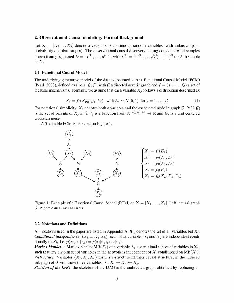
The underlying generative model of the data is assumed to be a Functional Causal Model (FCM)(Pearl, 2003), defined as a pair (G, f), with G a directed acyclic graph and f = (f1, . . . , fd) a set ofd causal mechanisms. Formally, we assume that each variable Xj follows a distribution described as:

Xj = fj(XPa(j;G), Ej), with Ej ∼ N (0, 1) for j = 1, . . . , d. (1)

For notational simplicity, Xj denotes both a variable and the associated node in graph G. Pa(j;G)is the set of parents of Xj in G, fj is a function from R|Pa(j;G)|+1 → R and Ej is a unit centeredGaussian noise.

A 5-variable FCM is depicted on Figure 1.

E1

f1

X1 E3E2 E4

f4

X4E5

f2 f3

X3

f5

X5

X2

X1 = f1(E1)

X2 = f2(X1, E2)

X3 = f3(X1, E3)

X4 = f4(E4)

X5 = f5(X3, X4, E5)

Figure 1: Example of a Functional Causal Model (FCM) on X = [X1, . . . , X5]. Left: causal graphG. Right: causal mechanisms.

2.2 Notations and Definitions

All notations used in the paper are listed in Appendix A. X\i denotes the set of all variables but Xi.Conditional independence: (Xi ⊥⊥Xj |Xk) means that variables Xi and Xj are independent condi-tionally to Xk, i.e. p(xi, xj |xk) = p(xi|xk)p(xj |xk).Markov blanket: a Markov blanket MB(Xi) of a variable Xi is a minimal subset of variables in X\isuch that any disjoint set of variables in the network is independent of Xi conditioned on MB(Xi).V-structure: Variables Xi, Xj , Xk form a v-structure iff their causal structure, in the inducedsubgraph of G with these three variables, is : Xi → Xk ← Xj .Skeleton of the DAG: the skeleton of the DAG is the undirected graph obtained by replacing all

3

edges by undirected edges.Markov equivalent DAG: two DAGs with same skeleton and same v-structures are said to be Markovequivalent (Pearl and Verma, 1991). A Markov equivalence class is represented by a CompletedPartially Directed Acyclic Graph (CPDAG) having both directed and undirected edges.

Variables Xi and Xj are said to be adjacent according to a CPDAG iff there exists an edgebetween both nodes. If directed, this edge models causal relationship Xi → Xj or Xj → Xi. Ifundirected, it models a causal relationship in either direction.

2.3 Causal Assumptions and Properties

In this paper, we make the following assumptions:

Acyclicity: The causal graph G (Equation (1)) is assumed to be a Directed Acyclic Graph (DAG).

Causal Markov Assumption (CMA): Noise variables Ej (Equation (1)) are assumed to be in-dependent from each other. This assumption together with the above DAG assumption yields theclassical causal Markov property, stating that all variables are independent of their non-effects(non descendants in the causal graph) conditionally to their direct causes (parents) (Spirtes et al.,2000). Under the causal Markov assumption, the distribution described by the FCM satisfies allconditional independence relations2 among variables in X via the notion of d-separation (Pearl,2009). Accordingly the joint distribution p(x) can be factorized as the product of the distributions ofeach variable conditionally on its parents in the graph:

p(x) =

d∏j=1

p(xj |xPa(j;G)) (2)

Causal Faithfulness Assumption (CFA): The joint distribution p(x) is assumed to be faithful tograph G, that is, every conditional independence relation that holds true according to p is entailed byG (Spirtes and Zhang, 2016). It follows from causal Markov and faithfulness assumptions that everycausal path in the graph corresponds to a dependency between variables, and vice versa.

Causal Sufficiency assumption (CSA): X is assumed to be causally sufficient, that is, a pair ofvariables Xi, Xj in X has no common cause external to X\i,j . In other words, we assume thatthere is no hidden confounder. This corresponds to making the assumption that the noise variablesEj for j = 1, .., d entering in Equation (1) are independent of each other.

2.4 Background

This section briefly presents a formal background of observational causal discovery, referring thereader to (Spirtes et al., 2000; Peters et al., 2017) for a comprehensive survey.

Observational causal discovery algorithms are structured along four categories:

I A first category of methods are score-based methods which aim to find the best CPDAG in thesense of some global score: using search heuristics, graph candidates are iteratively evaluatedusing a scoring criterion such as the AIC score or the BIC score and compared with the best

2. It must be noted however that the data might satisfy additional independence relations beyond those in the graph; seethe faithfulness assumption.

4

graph obtained so far. One of the most popular score-based method is the Greedy EquivalentSearch (GES) algorithm (Chickering, 2002). GES aims to find the best CPDAG in the senseof the Bayesian Information Criterion (BIC). The CPDAG space is navigated using localsearch operators, e.g. add edge, remove edge, and reverse edge. GES starts with an emptygraph. In a first forward phase, edges are iteratively added to greedily improve the globalscore. In a second backward phase, edges are iteratively removed to greedily improve thescore. Under CSA, CMA and CFA assumptions, GES identifies the true CPDAG in the largesample limit, if the score used is decomposable, score-equivalent and consistent (Chickering,2002). More recently, Ramsey et al. (2017) proposed a GES extension called Fast GreedyEquivalence Search (FGES) algorithm aimed to alleviate the computational cost of GES. Itleverages the decomposable structure of the graph to optimize all the subgraphs in parallel.This optimization greatly increases the computational efficiency of the algorithms, enablingscore-based methods to run on millions of variables.

II A second category of approaches are constraint-based methods leveraging conditional inde-pendence tests to identify a skeleton of the graph and v-structures, in order to output theCPDAG of the graph. One of the most famous constraint-based algorithm is the celebrated PCalgorithm (Spirtes et al., 1993): under CSA, CMA and CFA, and assuming that all conditionalindependences have been identified, PC returns the CPDAG of the functional causal model,respecting all v-structures. It has notably been shown that for graphs with bounded degree, thePC algorithm has a running time that is polynomial in the number of variables. When very fastindependence tests such as partial correlation tests are employed, the PC algorithm can handlehigh dimensional graphs (Kalisch and Buhlmann, 2007). For non Gaussian data generated withnon-linear mechanism and complex interactions between the variables, more powerful but alsomore time consuming tests have been proposed such has the Kernel Conditional Independencetest (KCI) (Zhang et al., 2012) leveraging the kernel-based Hilbert-Schmidt IndependenceCriterion (HSIC) (Gretton et al., 2005).

III The third category of approaches are hybrid algorithms which combine ideas from constraint-based and score-based algorithms. According to Nandy et al. (2015), such methods often use agreedy search like the GES method on a restricted search space for the sake of computationalefficiency. This restricted space is defined using conditional independence tests. The Max-MinHill climbing algorithm (MMHC) (Tsamardinos et al., 2006) firstly builds the skeleton of aBayesian network using conditional independence tests (using constraint-based approaches)and then performs a Bayesian-scoring hill-climbing search to orient the edges (using score-based approaches). The skeleton recovery phase, called Max-Min Parents and Children(MMPC) selects for each variable its parents and children in the variable set. Note that this taskis different from recovering the Markov blanket of variables as the spouses are not selected.The orientation phase is a hill-climbing greedy search involving 3 operators: add, delete andreverse edge.

IV The above-mentioned three categories of methods can learn at best the Markov equivalenceclass of the DAG which can be a significant limitation in some cases.3 Therefore, new methodsexploiting asymmetries or causal footprints in the data generative process have been proposed

3. In domains such as biology, the sought G graph is star-shaped and does not include v-structures. In such cases, thecited methods are unable to orient the edges (see section 6.5).

5

to uniquely identify the causal DAG. According to Quinn et al. (2011), the first approach inthis direction is LiNGAM (Shimizu et al., 2006). LiNGAM handles linear structural equationmodels on continuous variables, where each variable is modeled as the weighted sum of itsparents and noise. Assuming further that all noise variables are non-Gaussian, Shimizu et al.(2006) show that the causal structure is fully identifiable (all edges can be oriented).

Such methods, taking into account the full information from the observational data (Spirtes andZhang, 2016) such as data asymmetries induced by the causal directions, have been proposedand primarily applied to the bivariate DAG case,4 referred to as cause-effect pair problem(Hoyer et al., 2009; Daniusis et al., 2012; Mooij et al., 2016; Zhang and Hyvarinen, 2010).The reader is referred to Statnikov et al. (2012); Mooij et al. (2016); Guyon et al. (2019)for a thorough presentation of the bivariate problem. The pairwise additive model (ANM)has notably been extended in the multivariate setting with the causal additive models (CAM)(Buhlmann et al., 2014), able to recover the DAG when the structural equations are additive inthe variables and error terms.

As noted by Mooij et al. (2010), methods such as those presented by (Hoyer et al., 2009;Zhang and Hyvarinen, 2010) identify the DAG by restricting the class of admissible causalmechanisms. These models allow for theoretical identifiability, but the considered class ofmodels is often too restrictive for real-world data.

In order to overcome this restriction and build more expressive models, Mooij et al. (2010) haveproposed the fully non-parametric GPI approach. The key idea is to define appropriate priorson marginal distributions of the cause and on causal mechanisms in order to favor a modelof low complexity. This method was designed for the bivariate setting and has shown verygood results on a wide variety of data as it is not restricted to a specific class of mechanisms.The same type of Gaussian process inference model has been proposed by Friedman andNachman (2000) for the multivariate case. The authors use Gaussian process priors in order tolearn a wide variety of functional relations and they compare different candidate structures byevaluating likelihood scores.

The Causal Generative Neural Networks (CGNN) (Goudet et al., 2018) aims to continueon this path in the multivariate case. In CGNN, the causal mechanisms are modelled withgenerative neural networks. CGNN starts from a given skeleton and explore the space of DAGsusing a hill climbing algorithm aimed to optimize the global score of the network computed asthe Maximum Mean Discrepancy (MMD) (Gretton et al., 2007) between the true empiricaldistribution P and the generated distribution P .

The proposed SAM approach ambitions to combine the best of all the above: exploiting condi-tional independence relations as methods in the first three categories, and exploiting distributionalasymmetries, achieving some trade-off between model complexity and data fitting in the line of theGPI method (Mooij et al., 2010).

SAM aims at addressing the limitations of CGNN. The first limitation of CGNN is a quadraticcomputational complexity w.r.t. the size of the dataset, as its learning criterion is based on theMaximum Mean Discrepancy between the generated and the observed data. In contrast, SAM usesan adversarial learning approach (GAN) (Goodfellow et al., 2014) that scales linearly with the data

4. Note that in the bivariate case, both X → Y and Y → X DAGs are Markov equivalent; methods in categories I, IIand III do not apply.

6

size. Moreover as opposed to non-parametric methods such as kernel density estimates and nearestneighbor methods, adversarial learning suffers less from the curse of dimensionality, being able tomodel complex high-dimensional distributions (Lopez-Paz and Oquab, 2016; Karras et al., 2017).

The second limitation of CGNN is a scalability issue w.r.t. the number of variables, due to thegreedy search exploration in the space of DAGs, as all generative networks modelling the causalmechanisms in the causal graph must be retrained when a new graph structure is evaluated. SAMtackles this second issue by using an embedded framework for structure optimization, inspiredby (Zheng et al., 2018), where the mechanisms and the structure are simultaneously learned withinan end-to-end DAG learning framework.

3. Structural Agnostic model

This section presents the Structural Agnostic Model (SAM), within the space of generative neuralnetworks (NN). The originality of the approach is to implement an end-to-end search for an acyclicFunctional Causal Model (FCM, Equation 1) in the multivariate setting with a smooth trade-offbetween complexity and fit of the model.

3.1 Modeling causal mechanisms with conditional generative neural networks

The model search space includes all distributions q defined from a DAG G and causal mechanismsf = (f1, . . . , fd), with fj a deep neural network yielding a generative model of Xj from all othervariables in X (Figure 2). Formally:

• The d-dimensional vector of variables X is elementwise multiplied with binary vector aj =(a1,j , . . . ad,j) named structural gate. Coefficient ai,j is 1 iff variable Xi is used to generateXj (with ai,i set to 0 to avoid self-loops), that is, edge Xi → Xj is present in graph G, andXi is considered to be a cause of Xj . Otherwise, ai,j is set to 0. Two regularization termson ajs will be introduced in section 3.2 and 3.3 in order to enforce graph sparsity and graphacyclicity.

• At every evaluation of noise variable Ej , a value is drawn anew from distribution N (0, 1). Allthe noise variables Ej for j ∈ J1, dK are drawn from independent distributions.

3.1.1 DEEP NEURAL NETWORK CAUSAL MECHANISMS

Each fj is implemented as a H-hidden layer neural network, with nh nodes at the h-th hidden layerfor h = 1, ...,H . The input is of dimension n0 = d+ 1, the output is of dimension nH+1 = 1. Themathematical expression of each deep neural network is given by:

Xj = fj(X, Ej)

= Lj,H+1 σ Lj,H · · · σ Lj,1([aj X, Ej ])(3)

where aj X corresponds to the element wise product between the two vectors aj and X. Wedenote by [ajX, Ej ] the vector of size d+1 resulting of the concatenation between the vector ajXand Ej . Lj,h : Rnh−1 → Rnh is an affine linear map defined by Lj,h(x) = Wj,h · x + bj,h for givennh×nh−1 dimensional weight matrix Wj,h (with coefficients wj,hk,l 1≤k≤nh

1≤l≤nh−1

), nh dimensional bias

vector bj,h (with coefficients bj,hk 1≤k≤nh) and σ : Rnh →]− 1, 1[nh the element-wise nonlinear

7

activation map defined by σ(z) := (tanh(z1), ..., tanh(znh))T . We denote by θj , the set of all

weight matrices and bias vector of the neural network modelling the j-th causal mechanism fj :θj := (Wj,1,b1), (Wj,2,b2), . . . , (Wj,H+1,bH+1).

a1jX1

a(j−1)jXj−1

a(j+1)jXj+1

adjXd

1Ej

Xj

· · ·

· · ·

· · ·

· · ·

· · ·

· · ·

· · ·

X−j

Structural gates

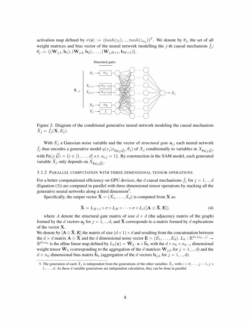
Figure 2: Diagram of the conditional generative neural network modeling the causal mechanismXj = fj(X, Ej).

With Ej a Gaussian noise variable and the vector of structural gate aj , each neural networkfj thus encodes a generative model q(xj |xPa(j;G)

, θj) of Xj conditionally to variables in XPa(j;G),

with Pa(j; G) = i ∈ [1, . . . , d] s.t. ai,j = 1. By construction in the SAM model, each generatedvariable Xj only depends on XPa(j;G)

.

3.1.2 PARALLEL COMPUTATION WITH THREE DIMENSIONAL TENSOR OPERATIONS

For a better computational efficiency on GPU devices, the d causal mechanisms fj for j = 1, .., d(Equation (3)) are computed in parallel with three dimensional tensor operations by stacking all thegenerative neural networks along a third dimension5.

Specifically, the output vector X = (X1, . . . , Xd) is computed from X as:

X = LH+1 σ LH · · · σ L1([A X,E]), (4)

where A denote the structural gate matrix of size d × d (the adjacency matrix of the graph)formed by the d vectors aj for j = 1, .., d, and X corresponds to a matrix formed by d replicationsof the vector X.We denote by [AX,E] the matrix of size (d+1)×d and resulting from the concatenation betweenthe d× d matrix A X and the d dimensional noise vector E = (E1, . . . , Ed). Lh : Rd×(nh−1) →Rd×nh is the affine linear map defined by Lh(x) = Wh ·x+ bh with the d×nh×nh−1 dimensionalweight tensor Wh (corresponding to the aggregation of the d matrices Wj,h for j = 1, .., d) and thed× nh dimensional bias matrix bh (aggregation of the d vectors bj,h for j = 1, .., d).

5. The generation of each Xj is independent from the generations of the other variables Xi, with i = 0, . . . , j − 1, j +1, . . . , d. As these d variable generations are independent calculation, they can be done in parallel.

8

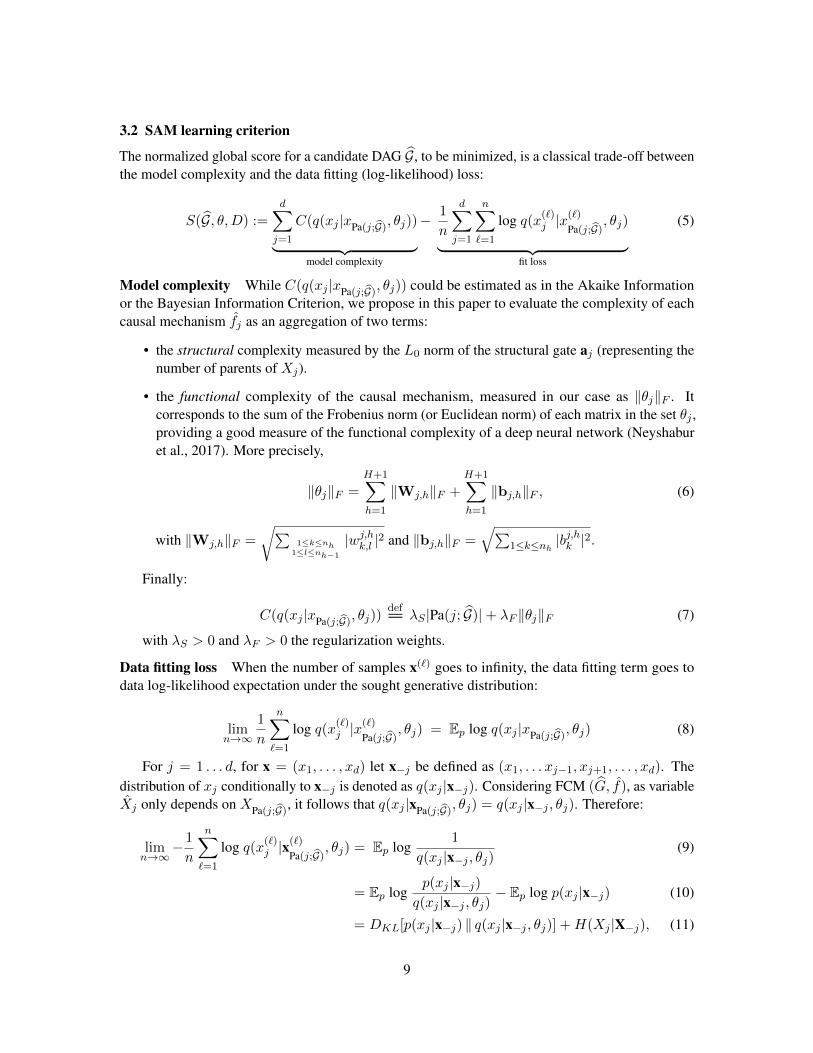
3.2 SAM learning criterion

The normalized global score for a candidate DAG G, to be minimized, is a classical trade-off betweenthe model complexity and the data fitting (log-likelihood) loss:

S(G, θ,D) :=

d∑j=1

C(q(xj |xPa(j;G), θj))︸ ︷︷ ︸

model complexity

− 1

n

d∑j=1

n∑`=1

log q(x(`)j |x

(`)

Pa(j;G), θj)︸ ︷︷ ︸

fit loss

(5)

Model complexity While C(q(xj |xPa(j;G), θj)) could be estimated as in the Akaike Information

or the Bayesian Information Criterion, we propose in this paper to evaluate the complexity of eachcausal mechanism fj as an aggregation of two terms:

• the structural complexity measured by the L0 norm of the structural gate aj (representing thenumber of parents of Xj).

• the functional complexity of the causal mechanism, measured in our case as ‖θj‖F . Itcorresponds to the sum of the Frobenius norm (or Euclidean norm) of each matrix in the set θj ,providing a good measure of the functional complexity of a deep neural network (Neyshaburet al., 2017). More precisely,

‖θj‖F =H+1∑h=1

‖Wj,h‖F +H+1∑h=1

‖bj,h‖F , (6)

with ‖Wj,h‖F =√∑

1≤k≤nh1≤l≤nh−1

|wj,hk,l |2 and ‖bj,h‖F =√∑

1≤k≤nh|bj,hk |2.

Finally:

C(q(xj |xPa(j;G), θj))

def= λS |Pa(j; G)|+ λF ‖θj‖F (7)

with λS > 0 and λF > 0 the regularization weights.

Data fitting loss When the number of samples x(`) goes to infinity, the data fitting term goes todata log-likelihood expectation under the sought generative distribution:

limn→∞

1

n

n∑`=1

log q(x(`)j |x

(`)

Pa(j;G), θj) = Ep log q(xj |xPa(j;G)

, θj) (8)

For j = 1 . . . d, for x = (x1, . . . , xd) let x−j be defined as (x1, . . . xj−1, xj+1, . . . , xd). Thedistribution of xj conditionally to x−j is denoted as q(xj |x−j). Considering FCM (G, f), as variableXj only depends on XPa(j;G)

, it follows that q(xj |xPa(j;G), θj) = q(xj |x−j , θj). Therefore:

limn→∞

− 1

n

n∑`=1

log q(x(`)j |x

(`)

Pa(j;G), θj) = Ep log

1

q(xj |x−j , θj)(9)

= Ep logp(xj |x−j)

q(xj |x−j , θj)− Ep log p(xj |x−j) (10)

= DKL[p(xj |x−j) ‖ q(xj |x−j , θj)] +H(Xj |X−j), (11)

9

with DKL[p(xj |x−j) ‖ q(xj |x−j , θj)] the Kullback-Leibler divergence between the true condi-tional distribution p(xj |x−j) and q(xj |x−j , θj), and H(Xj |X−j) the constant, domain-dependententropy of Xj conditionally to X−j (neglected in the following).

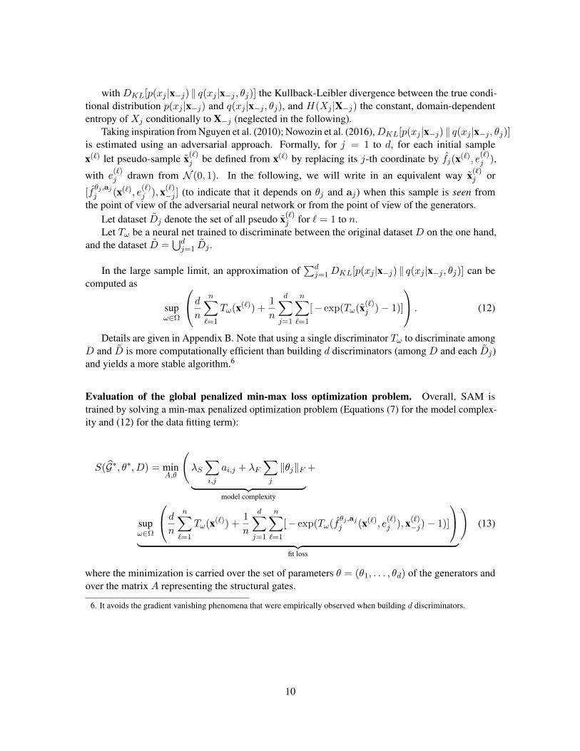
Taking inspiration from Nguyen et al. (2010); Nowozin et al. (2016),DKL[p(xj |x−j) ‖ q(xj |x−j , θj)]is estimated using an adversarial approach. Formally, for j = 1 to d, for each initial samplex(`) let pseudo-sample x(`)

j be defined from x(`) by replacing its j-th coordinate by fj(x(`), e(`)j ),

with e(`)j drawn from N (0, 1). In the following, we will write in an equivalent way x(`)

j or

[fθj ,aj

j (x(`), e(`)j ), x(`)

−j ] (to indicate that it depends on θj and aj) when this sample is seen fromthe point of view of the adversarial neural network or from the point of view of the generators.

Let dataset Dj denote the set of all pseudo x(`)j for ` = 1 to n.

Let Tω be a neural net trained to discriminate between the original dataset D on the one hand,and the dataset D =

⋃dj=1 Dj .

In the large sample limit, an approximation of∑d

j=1DKL[p(xj |x−j) ‖ q(xj |x−j , θj)] can becomputed as

supω∈Ω

d

n

n∑`=1

Tω(x(`)) +1

n

d∑j=1

n∑`=1

[− exp(Tω(x(`)j )− 1)]

. (12)

Details are given in Appendix B. Note that using a single discriminator Tω to discriminate amongD and D is more computationally efficient than building d discriminators (among D and each Dj)and yields a more stable algorithm.6

Evaluation of the global penalized min-max loss optimization problem. Overall, SAM istrained by solving a min-max penalized optimization problem (Equations (7) for the model complex-ity and (12) for the data fitting term):

S(G∗, θ∗, D) = minA,θ

(λS∑i,j

ai,j + λF∑j

‖θj‖F︸ ︷︷ ︸model complexity

+

supω∈Ω

d

n

n∑`=1

Tω(x(`)) +1

n

d∑j=1

n∑`=1

[− exp(Tω(fθj ,aj

j (x(`), e(`)j ), x(`)

−j)− 1)]

︸ ︷︷ ︸

fit loss

)(13)

where the minimization is carried over the set of parameters θ = (θ1, . . . , θd) of the generators andover the matrix A representing the structural gates.

6. It avoids the gradient vanishing phenomena that were empirically observed when building d discriminators.

10

a21X2

a31X3

a41X4

1E1

X1

· · ·· · ·· · ·· · ·· · ·

X−1

a14X1

a24X2

a34X3

1E4

X4

· · ·· · ·· · ·· · ·· · ·

X−4

D1

D4

∼ DKL[p(x1|x−1)|q(x1|x−1, θ1)]. . .∼ DKL[p(x4|x−4)|q(xj |x−4, θ4)]

D: True Data

Structural gates

Generators f1 . . . f4 Generated data Discriminator Tω

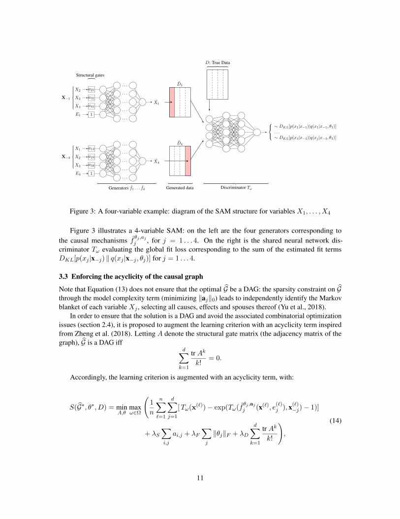
Figure 3: A four-variable example: diagram of the SAM structure for variables X1, . . . , X4

Figure 3 illustrates a 4-variable SAM: on the left are the four generators corresponding tothe causal mechanisms fθj ,ajj , for j = 1 . . . 4. On the right is the shared neural network dis-criminator Tω evaluating the global fit loss corresponding to the sum of the estimated fit termsDKL[p(xj |x−j) ‖ q(xj |x−j , θj)] for j = 1 . . . 4.

3.3 Enforcing the acyclicity of the causal graph

Note that Equation (13) does not ensure that the optimal G be a DAG: the sparsity constraint on Gthrough the model complexity term (minimizing ‖aj‖0) leads to independently identify the Markovblanket of each variable Xj , selecting all causes, effects and spouses thereof (Yu et al., 2018).

In order to ensure that the solution is a DAG and avoid the associated combinatorial optimizationissues (section 2.4), it is proposed to augment the learning criterion with an acyclicity term inspiredfrom Zheng et al. (2018). Letting A denote the structural gate matrix (the adjacency matrix of thegraph), G is a DAG iff

d∑k=1

tr Ak

k!= 0.

Accordingly, the learning criterion is augmented with an acyclicity term, with:

S(G∗, θ∗, D) = minA,θ

maxω∈Ω

(1

n

n∑`=1

d∑j=1

[Tω(x(`))− exp(Tω(fθj ,aj

j (x(`), e(`)j ), x(`)

−j)− 1)]

+ λS∑i,j

ai,j + λF∑j

‖θj‖F + λD

d∑k=1

tr Ak

k!

),

(14)

11

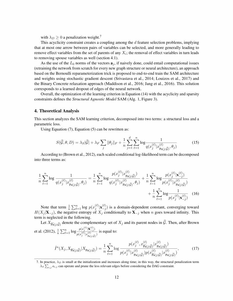
with λD ≥ 0 a penalization weight.7

This acyclicity constraint creates a coupling among the d feature selection problems, implyingthat at most one arrow between pairs of variables can be selected, and more generally leading toremove effect variables from the set of parents of any Xi; the removal of effect variables in turn leadsto removing spouse variables as well (section 4.1).

As the use of the L0 norms of the vectors aj , if naively done, could entail computational issues(retraining the network from scratch for every new graph structure or neural architecture), an approachbased on the Bernoulli reparameterization trick is proposed to end-to-end train the SAM architectureand weights using stochastic gradient descent (Srivastava et al., 2014; Louizos et al., 2017) andthe Binary Concrete relaxation approach (Maddison et al., 2016; Jang et al., 2016). This solutioncorresponds to a learned dropout of edges of the neural network.

Overall, the optimization of the learning criterion in Equation (14) with the acyclicity and sparsityconstraints defines the Structural Agnostic Model SAM (Alg. 1, Figure 3).

4. Theoretical Analysis

This section analyzes the SAM learning criterion, decomposed into two terms: a structural loss and aparametric loss.

Using Equation (7), Equation (5) can be rewritten as:

S(G, θ,D) = λS |G|+ λF∑j

‖θj‖F +1

n

d∑j=1

n∑`=1

log1

q(x(`)j |x

(`)

Pa(j;G), θj)

(15)

According to (Brown et al., 2012), each scaled conditional log-likelihood term can be decomposedinto three terms as:

1

n

n∑`=1

log1

q(x(`)j |x

(`)

Pa(j;G), θj)

=1

n

n∑`=1

logp(x

(`)j |x

(`)

Pa(j;G))

q(x(`)j |x

(`)

Pa(j;G), θj)

+1

n

n∑`=1

logp(x

(`)j |x

(`)−j)

p(x(`)j |x

(`)

Pa(j;G))

+1

n

n∑`=1

log1

p(x(`)j |x

(`)−j)

(16)

Note that term 1n

∑n`=1 log p(x(`)

j |x(`)−j) is a domain-dependent constant, converging toward

H(Xj |X−j), the negative entropy of Xj conditionally to X−j when n goes toward infinity. Thisterm is neglected in the following.

Let XPa(j;G)denote the complementary set of Xj and its parent nodes in G. Then, after Brown

et al. (2012), 1n

∑n`=1 log

p(x(`)j |x(`)

−j)

p(x(`)j |x

(`)

Pa(j;G))

is equal to:

In(Xj , XPa(j;G)|XPa(j;G)

) =1

n

n∑`=1

logp(x

(`)j , x

(`)

Pa(j;G)|x(`)

Pa(j;G))

p(x(`)j |x

(`)

Pa(j;G))p(x

(`)

Pa(j;G)|x(`)

Pa(j;G)), (17)

7. In practice, λD is small at the initialization and increases along time; in this way, the structural penalization termλS

∑i,j ai,j can operate and prune the less relevant edges before considering the DAG constraint.

12

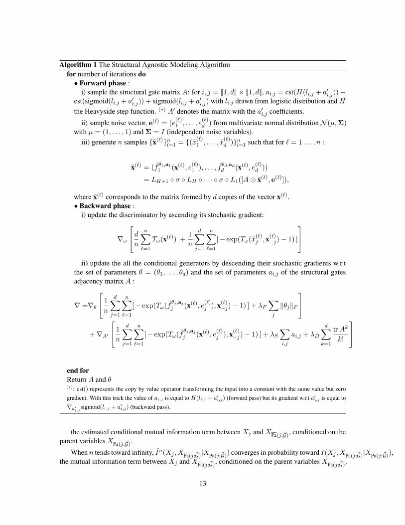
Algorithm 1 The Structural Agnostic Modeling Algorithmfor number of iterations do• Forward phase :

i) sample the structural gate matrix A: for i, j = J1, dK× J1, dK, ai,j = cst(H(li,j + a′i,j))−cst(sigmoid(li,j + a′i,j)) + sigmoid(li,j + a′i,j) with li,j drawn from logistic distribution and Hthe Heavyside step function. (∗) A′ denotes the matrix with the a′i,j coefficients.

ii) sample noise vector, e(`) = (e(`)1 , . . . , e

(`)d ) from multivariate normal distributionN (µ,Σ)

with µ = (1, . . . , 1) and Σ = I (independent noise variables).iii) generate n samples x(`)nl=1 = (x(`)

1 , . . . , x(`)d )nl=1 such that for ` = 1 . . . , n :

x(`) = (fθ1,a11 (x(`), e

(`)1 ), . . . , fθd,ad

d (x(`), e(`)d ))

= LH+1 σ LH · · · σ L1([A x(`), e(`)]),

where x(`) corresponds to the matrix formed by d copies of the vector x(`).• Backward phase :

i) update the discriminator by ascending its stochastic gradient:

∇ω

dn

n∑`=1

Tω(x(`)) +1

n

d∑j=1

n∑`=1

[− exp(Tω(x(`)j , x(`)

−j)− 1) ]

ii) update the all the conditional generators by descending their stochastic gradients w.r.t

the set of parameters θ = (θ1, . . . , θd) and the set of parameters ai,j of the structural gatesadjacency matrix A :

∇ =∇θ

1

n

d∑j=1

n∑`=1

[− exp(Tω(fθj ,aj

j (x(`), e(`)j ), x(`)

−j)− 1) ] + λF∑j

‖θj‖F

+∇A′

1

n

d∑j=1

n∑`=1

[− exp(Tω(fθj ,aj

j (x(`), e(`)j ), x(`)

−j)− 1) ] + λS∑i,j

ai,j + λD

d∑k=1

tr Ak

k!

end forReturn A and θ(∗): cst() represents the copy by value operator transforming the input into a constant with the same value but zero

gradient. With this trick the value of ai,j is equal to H(li,j + a′i,j) (forward pass) but its gradient w.r.t a′i,j is equal to

∇a′i,j

sigmoid(li,j + a′i,j) (backward pass).

the estimated conditional mutual information term between Xj and XPa(j;G), conditioned on the

parent variables XPa(j;G).

When n tends toward infinity, In(Xj , XPa(j;G)|XPa(j;G)

) converges in probability toward I(Xj , XPa(j;G)|XPa(j;G)

),the mutual information term between Xj and XPa(j;G)

, conditioned on the parent variables XPa(j;G).

13

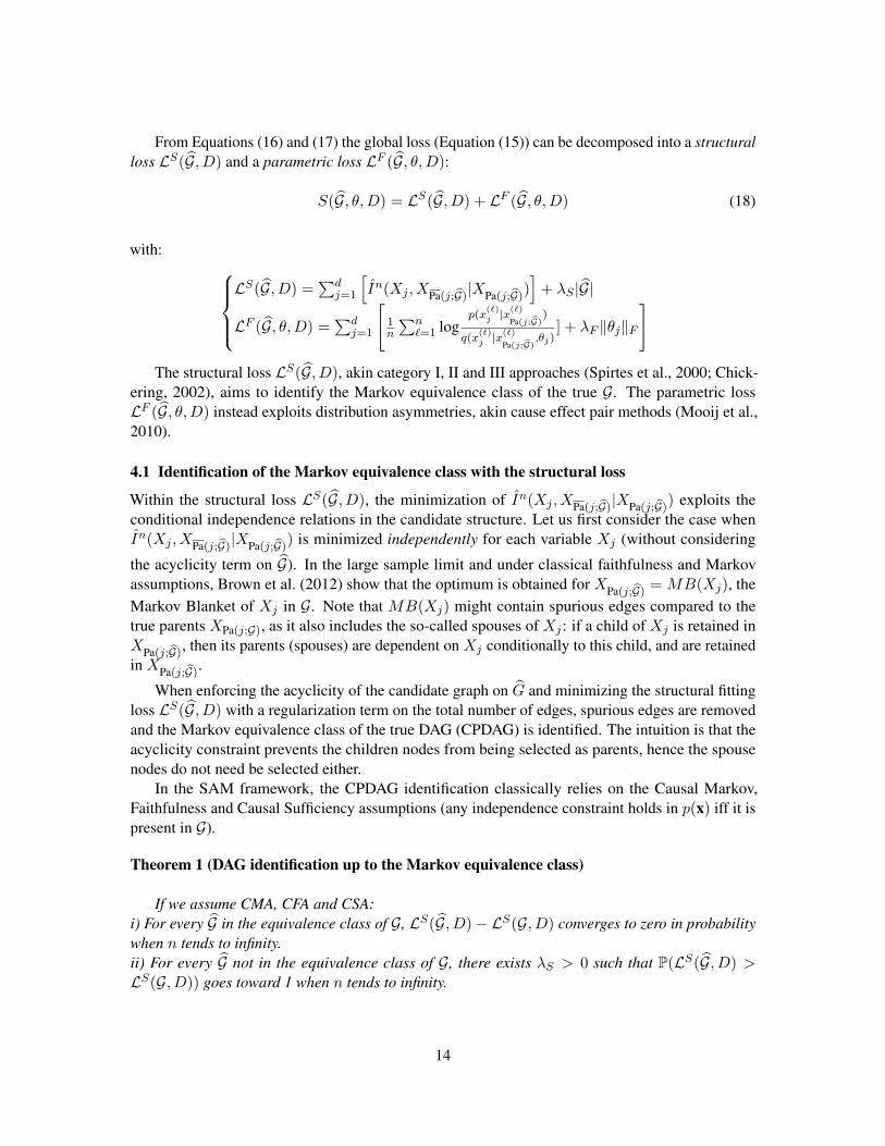
From Equations (16) and (17) the global loss (Equation (15)) can be decomposed into a structuralloss LS(G, D) and a parametric loss LF (G, θ,D):

S(G, θ,D) = LS(G, D) + LF (G, θ,D) (18)

with: LS(G, D) =

∑dj=1

[In(Xj , XPa(j;G)

|XPa(j;G))]

+ λS |G|

LF (G, θ,D) =∑d

j=1

[1n

∑n`=1 log

p(x(`)j |x

(`)

Pa(j;G))

q(x(`)j |x

(`)

Pa(j;G),θj)

] + λF ‖θj‖F]

The structural loss LS(G, D), akin category I, II and III approaches (Spirtes et al., 2000; Chick-ering, 2002), aims to identify the Markov equivalence class of the true G. The parametric lossLF (G, θ,D) instead exploits distribution asymmetries, akin cause effect pair methods (Mooij et al.,2010).

4.1 Identification of the Markov equivalence class with the structural loss

Within the structural loss LS(G, D), the minimization of In(Xj , XPa(j;G)|XPa(j;G)

) exploits theconditional independence relations in the candidate structure. Let us first consider the case whenIn(Xj , XPa(j;G)

|XPa(j;G)) is minimized independently for each variable Xj (without considering

the acyclicity term on G). In the large sample limit and under classical faithfulness and Markovassumptions, Brown et al. (2012) show that the optimum is obtained for XPa(j;G)

= MB(Xj), theMarkov Blanket of Xj in G. Note that MB(Xj) might contain spurious edges compared to thetrue parents XPa(j;G), as it also includes the so-called spouses of Xj : if a child of Xj is retained inXPa(j;G)

, then its parents (spouses) are dependent on Xj conditionally to this child, and are retainedin XPa(j;G)

.

When enforcing the acyclicity of the candidate graph on G and minimizing the structural fittingloss LS(G, D) with a regularization term on the total number of edges, spurious edges are removedand the Markov equivalence class of the true DAG (CPDAG) is identified. The intuition is that theacyclicity constraint prevents the children nodes from being selected as parents, hence the spousenodes do not need be selected either.

In the SAM framework, the CPDAG identification classically relies on the Causal Markov,Faithfulness and Causal Sufficiency assumptions (any independence constraint holds in p(x) iff it ispresent in G).

Theorem 1 (DAG identification up to the Markov equivalence class)

If we assume CMA, CFA and CSA:i) For every G in the equivalence class of G, LS(G, D)− LS(G, D) converges to zero in probabilitywhen n tends to infinity.ii) For every G not in the equivalence class of G, there exists λS > 0 such that P(LS(G, D) >LS(G, D)) goes toward 1 when n tends to infinity.

14

Proof in Appendix C

Theoretical and experimental illustrations of the results on the toy 3-variable skeleton A−B−Care presented in Appendix C.

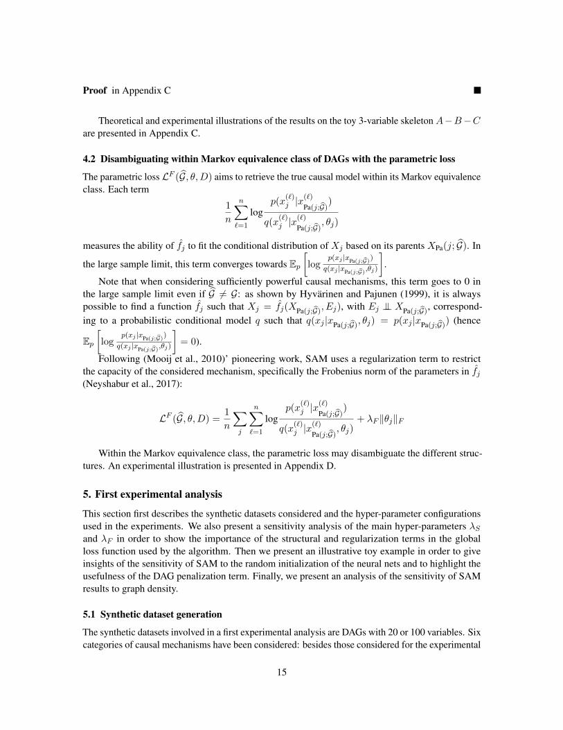
4.2 Disambiguating within Markov equivalence class of DAGs with the parametric loss

The parametric loss LF (G, θ,D) aims to retrieve the true causal model within its Markov equivalenceclass. Each term

1

n

n∑`=1

logp(x

(`)j |x

(`)

Pa(j;G))

q(x(`)j |x

(`)

Pa(j;G), θj)

measures the ability of fj to fit the conditional distribution of Xj based on its parents XPa(j; G). In

the large sample limit, this term converges towards Ep[log

p(xj |xPa(j;G))

q(xj |xPa(j;G),θj)

].

Note that when considering sufficiently powerful causal mechanisms, this term goes to 0 inthe large sample limit even if G 6= G: as shown by Hyvarinen and Pajunen (1999), it is alwayspossible to find a function fj such that Xj = fj(XPa(j;G)

, Ej), with Ej ⊥⊥ XPa(j;G), correspond-

ing to a probabilistic conditional model q such that q(xj |xPa(j;G), θj) = p(xj |xPa(j;G)

) (hence

Ep[log

p(xj |xPa(j;G))

q(xj |xPa(j;G),θj)

]= 0).

Following (Mooij et al., 2010)’ pioneering work, SAM uses a regularization term to restrictthe capacity of the considered mechanism, specifically the Frobenius norm of the parameters in fj(Neyshabur et al., 2017):

LF (G, θ,D) =1

n

∑j

n∑`=1

logp(x

(`)j |x

(`)

Pa(j;G))

q(x(`)j |x

(`)

Pa(j;G), θj)

+ λF ‖θj‖F

Within the Markov equivalence class, the parametric loss may disambiguate the different struc-tures. An experimental illustration is presented in Appendix D.

5. First experimental analysis

This section first describes the synthetic datasets considered and the hyper-parameter configurationsused in the experiments. We also present a sensitivity analysis of the main hyper-parameters λSand λF in order to show the importance of the structural and regularization terms in the globalloss function used by the algorithm. Then we present an illustrative toy example in order to giveinsights of the sensitivity of SAM to the random initialization of the neural nets and to highlight theusefulness of the DAG penalization term. Finally, we present an analysis of the sensitivity of SAMresults to graph density.

5.1 Synthetic dataset generation

The synthetic datasets involved in a first experimental analysis are DAGs with 20 or 100 variables. Sixcategories of causal mechanisms have been considered: besides those considered for the experimental

15

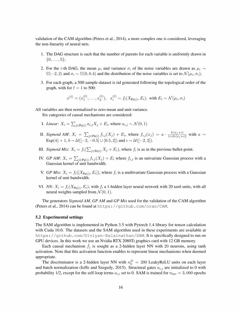
validation of the CAM algorithm (Peters et al., 2014), a more complex one is considered, leveragingthe non-linearity of neural nets.

1. The DAG structure is such that the number of parents for each variable is uniformly drawn in0, . . . , 5;

2. For the i-th DAG, the mean µi and variance σi of the noise variables are drawn as µi ∼U(−2, 2) and σi ∼ U(0, 0.4) and the distribution of the noise variables is set to N (µi, σi);

3. For each graph, a 500 sample-dataset is iid generated following the topological order of thegraph, with for ` = 1 to 500:

x(`) = (x(`)1 , . . . , x

(`)d ), x

(`)i ∼ fi(XPa(i), Ei), with Ei ∼ N (µi, σi)

All variables are then normalized to zero-mean and unit-variance.Six categories of causal mechanisms are considered:

I. Linear: Xi =∑

j∈Pa(i) ai,jXj + Ei, where ai,j ∼ N (0, 1)

II. Sigmoid AM: Xi =∑

j∈Pa(i) fi,j(Xj) + Ei, where fi,j(xj) = a · b·(xj+c)1+|b·(xj+c)| with a ∼

Exp(4) + 1, b ∼ U([−2,−0.5] ∪ [0.5, 2]) and c ∼ U([−2, 2]).

III. Sigmoid Mix: Xi = fi(∑

j∈Pa(i)Xj + Ei), where fi is as in the previous bullet-point.

IV. GP AM: Xi =∑

j∈Pa(i) fi,j(Xj) + Ei where fi,j is an univariate Gaussian process with aGaussian kernel of unit bandwidth.

V. GP Mix: Xi = fi([XPa(i), Ei]), where fi is a multivariate Gaussian process with a Gaussiankernel of unit bandwidth.

VI. NN: Xi = fi(XPa(i), Ei), with fi a 1-hidden layer neural network with 20 tanh units, with allneural weights sampled from N (0, 1).

The generators Sigmoid AM, GP AM and GP Mix used for the validation of the CAM algorithm(Peters et al., 2014) can be found at https://github.com/cran/CAM.

5.2 Experimental settings

The SAM algorithm is implemented in Python 3.5 with Pytorch 1.4 library for tensor calculationwith Cuda 10.0. The datasets and the SAM algorithm used in these experiments are available athttps://github.com/Diviyan-Kalainathan/SAM. It is specifically designed to run onGPU devices. In this work we use an Nvidia RTX 2080Ti graphics card with 12 GB memory.

Each causal mechanism fj is sought as a 2-hidden layer NN with 20 neurons, using tanhactivation. Note that this activation function enables to represent linear mechanisms when deemedappropriate.

The discriminator is a 2-hidden layer NN with nDh = 200 LeakyReLU units on each layerand batch normalization (Ioffe and Szegedy, 2015). Structural gates ai,j are initialized to 0 withprobability 1/2, except for the self-loop terms ai,i set to 0. SAM is trained for niter = 3, 000 epochs

16

using Adam (Kingma and Ba, 2014) with initial learning rate 0.01 for the generators and 0.001 forthe discriminator.

In all experiments, we set the acyclicity penalization weight to

λD =

0 if t < 1, 5000.01× (t− 1, 500) otherwise

(19)

with t the number of epochs: the first half of the training does not take into account the acyclicityconstraint and focuses on the identification of the Markov blankets for each variable; the acyclicityconstraint intervenes in the second half of the run and its weight increases along time. At the end ofthe learning, the value of λD takes a sufficiently high value such that all resulting graphs presentedin the experiments of this section are acyclic graphs.

To identify appropriate values for the main sensitive SAM parameters λS (respectively λF ), weapplied a grid search on domain J0, 2K (resp. J0, 0.002K) while keeping the other parameters withtheir default values ; each candidate (λS , λF ) is assessed over the problem set involving 20 variablessynthetic graphs in each of the above-mentioned six categories.

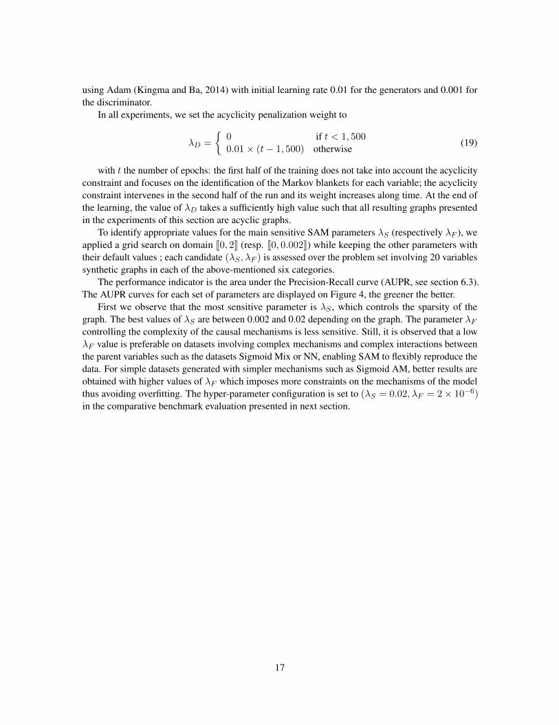
The performance indicator is the area under the Precision-Recall curve (AUPR, see section 6.3).The AUPR curves for each set of parameters are displayed on Figure 4, the greener the better.

First we observe that the most sensitive parameter is λS , which controls the sparsity of thegraph. The best values of λS are between 0.002 and 0.02 depending on the graph. The parameter λFcontrolling the complexity of the causal mechanisms is less sensitive. Still, it is observed that a lowλF value is preferable on datasets involving complex mechanisms and complex interactions betweenthe parent variables such as the datasets Sigmoid Mix or NN, enabling SAM to flexibly reproduce thedata. For simple datasets generated with simpler mechanisms such as Sigmoid AM, better results areobtained with higher values of λF which imposes more constraints on the mechanisms of the modelthus avoiding overfitting. The hyper-parameter configuration is set to (λS = 0.02, λF = 2× 10−6)in the comparative benchmark evaluation presented in next section.

17

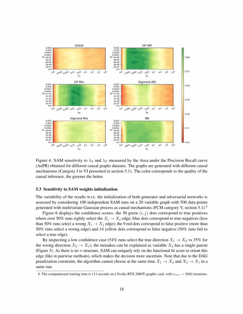
Figure 4: SAM sensitivity to λS and λF measured by the Area under the Precision Recall curve(AuPR) obtained for different causal graphs datasets. The graphs are generated with different causalmechanisms (Category I to VI presented in section 5.1). The color corresponds to the quality of thecausal inference, the greener the better.

5.3 Sensitivity to SAM weights initialization

The variability of the results w.r.t. the initialization of both generator and adversarial networks isassessed by considering 100 independent SAM runs on a 20 variable graph with 500 data pointsgenerated with multivariate Gaussian process as causal mechanisms (FCM category V, section 5.1).8

Figure 6 displays the confidence scores: the 30 green (i, j) dots correspond to true positiveswhere over 50% runs rightly select the Xi → Xj edge; blue dots correspond to true negatives (lessthan 50% runs select a wrong Xi → Xj edge); the 9 red dots correspond to false positive (more than50% runs select a wrong edge) and 14 yellow dots correspond to false negative (50% runs fail toselect a true edge).

By inspecting a low confidence case (54% runs select the true direction X1 → X2 vs 35% forthe wrong direction X2 → X1), the mistakes can be explained as variable X2 has a single parent(Figure 5). As there is no v-structure, SAM can uniquely rely on the functional fit score to orient thisedge (like in pairwise methods), which makes the decision more uncertain. Note that due to the DAGpenalization constraint, the algorithm cannot choose at the same time X1 → X2 and X2 → X1 in asame run.

8. The computational training time is 113 seconds on a Nvidia RTX 2080Ti graphic card, with niter = 3000 iterations.

18

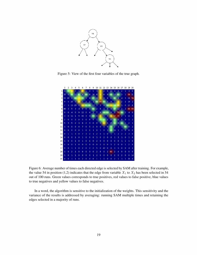
Figure 5: View of the first four variables of the true graph.

Figure 6: Average number of times each directed edge is selected by SAM after training. For example,the value 54 in position (1,2) indicates that the edge from variable X1 to X2 has been selected in 54out of 100 runs. Green values corresponds to true positives, red values to false positive, blue valuesto true negatives and yellow values to false negatives.

In a word, the algorithm is sensitive to the initialization of the weights. This sensitivity and thevariance of the results is addressed by averaging: running SAM multiple times and retaining theedges selected in a majority of runs.

19

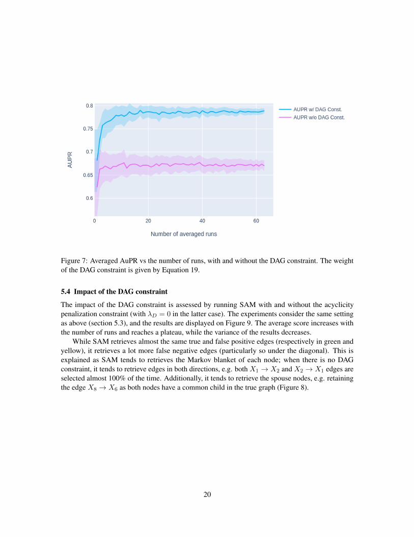
Figure 7: Averaged AuPR vs the number of runs, with and without the DAG constraint. The weightof the DAG constraint is given by Equation 19.

5.4 Impact of the DAG constraint

The impact of the DAG constraint is assessed by running SAM with and without the acyclicitypenalization constraint (with λD = 0 in the latter case). The experiments consider the same settingas above (section 5.3), and the results are displayed on Figure 9. The average score increases withthe number of runs and reaches a plateau, while the variance of the results decreases.

While SAM retrieves almost the same true and false positive edges (respectively in green andyellow), it retrieves a lot more false negative edges (particularly so under the diagonal). This isexplained as SAM tends to retrieves the Markov blanket of each node; when there is no DAGconstraint, it tends to retrieve edges in both directions, e.g. both X1 → X2 and X2 → X1 edges areselected almost 100% of the time. Additionally, it tends to retrieve the spouse nodes, e.g. retainingthe edge X8 → X6 as both nodes have a common child in the true graph (Figure 8).

20

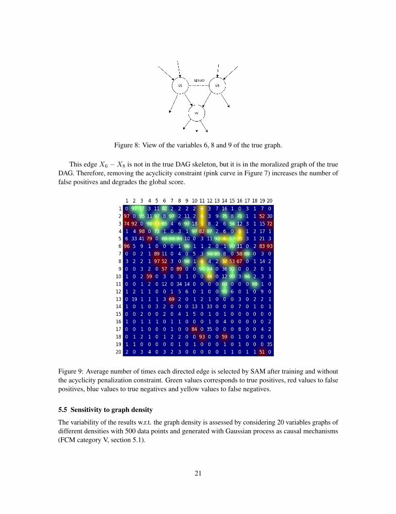
Figure 8: View of the variables 6, 8 and 9 of the true graph.

This edge X6 −X8 is not in the true DAG skeleton, but it is in the moralized graph of the trueDAG. Therefore, removing the acyclicity constraint (pink curve in Figure 7) increases the number offalse positives and degrades the global score.

Figure 9: Average number of times each directed edge is selected by SAM after training and withoutthe acyclicity penalization constraint. Green values corresponds to true positives, red values to falsepositives, blue values to true negatives and yellow values to false negatives.

5.5 Sensitivity to graph density

The variability of the results w.r.t. the graph density is assessed by considering 20 variables graphs ofdifferent densities with 500 data points and generated with Gaussian process as causal mechanisms(FCM category V, section 5.1).

21

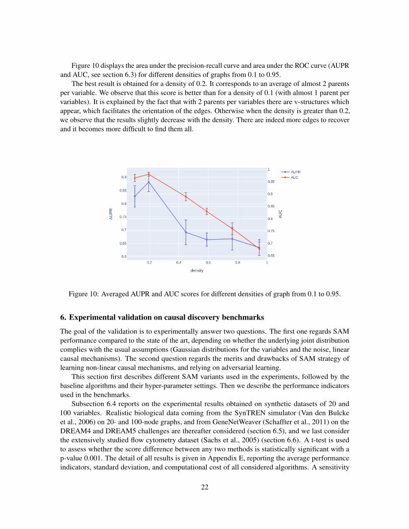
Figure 10 displays the area under the precision-recall curve and area under the ROC curve (AUPRand AUC, see section 6.3) for different densities of graphs from 0.1 to 0.95.

The best result is obtained for a density of 0.2. It corresponds to an average of almost 2 parentsper variable. We observe that this score is better than for a density of 0.1 (with almost 1 parent pervariables). It is explained by the fact that with 2 parents per variables there are v-structures whichappear, which facilitates the orientation of the edges. Otherwise when the density is greater than 0.2,we observe that the results slightly decrease with the density. There are indeed more edges to recoverand it becomes more difficult to find them all.

Figure 10: Averaged AUPR and AUC scores for different densities of graph from 0.1 to 0.95.

6. Experimental validation on causal discovery benchmarks

The goal of the validation is to experimentally answer two questions. The first one regards SAMperformance compared to the state of the art, depending on whether the underlying joint distributioncomplies with the usual assumptions (Gaussian distributions for the variables and the noise, linearcausal mechanisms). The second question regards the merits and drawbacks of SAM strategy oflearning non-linear causal mechanisms, and relying on adversarial learning.

This section first describes different SAM variants used in the experiments, followed by thebaseline algorithms and their hyper-parameter settings. Then we describe the performance indicatorsused in the benchmarks.

Subsection 6.4 reports on the experimental results obtained on synthetic datasets of 20 and100 variables. Realistic biological data coming from the SynTREN simulator (Van den Bulckeet al., 2006) on 20- and 100-node graphs, and from GeneNetWeaver (Schaffter et al., 2011) on theDREAM4 and DREAM5 challenges are thereafter considered (section 6.5), and we last considerthe extensively studied flow cytometry dataset (Sachs et al., 2005) (section 6.6). A t-test is usedto assess whether the score difference between any two methods is statistically significant with ap-value 0.001. The detail of all results is given in Appendix E, reporting the average performanceindicators, standard deviation, and computational cost of all considered algorithms. A sensitivity

22

analysis to the sample size is given in Appendix F. Appendix G reports a comparison of the SAMalgorithm with pairwise methods for the task of Markov equivalence class disambiguation. Finally,an analysis of the robustness of the various methods to non-Gaussian noise is presented in appendixH.

For convenience and reproducibility, all considered algorithms have been integrated in thepublicly available CausalDiscovery Toolbox,9 including the most recent baseline versions at the timeof the experiments.

6.1 Different SAM variants

In the benchmarks, four variants have been considered: the full SAM (Alg. 1) and three lesionedvariants designed to assess the benefits of non-linear mechanisms and adversarial training. Specifi-cally, SAM-lin desactivates the non-linear option and only implements linear causal mechanisms,replacing Equation (3) with:

Xj =

d∑i=1

Wj,iaj,iXi +Wj,d+1Ej +Wj,0 (20)

A second variant, SAM-mse, replaces the adversarial loss with a standard mean-square errorloss, replacing the f-gan term in Equation (24) with 1

n

∑dj=1

∑n`=1(x

(`)j − x

(`)j )2.

A third variant, SAM-lin-mse, involves both linear mechanisms and mean square error losses.

6.2 Baseline algorithms

The following algorithms have been used, with their default parameters: the score-based methodsGES (Chickering, 2002) and GIES (Hauser and Buhlmann, 2012) with Gaussian scores; the hybridmethod MMHC (Tsamardinos et al., 2006), the L1 penalized method for causal discovery CCDr(Aragam and Zhou, 2015), the LiNGAM algorithm (Shimizu et al., 2006) and the causal additivemodel CAM (Peters et al., 2014). Lastly, the PC algorithm (Spirtes et al., 2000) has been consideredwith four conditional independence tests in the Gaussian and non-parametric settings:

• PC-Gauss: using a Gaussian conditional independence test on z-scores;

• PC-HSIC: using the HSIC independence test (Zhang et al., 2012) with a Gamma null distribu-tion (Gretton et al., 2005);

• PC-RCIT: using the Randomized Conditional Independence Test (RCIT) with random Fourierfeatures (Strobl et al., 2017);

• PC-RCOT: the Randomized conditional Correlation Test (RCOT) (Strobl et al., 2017).

PC,10 GES and LINGAM versions are those of the pcalg package (Kalisch et al., 2012). MMHCis implemented with the bnlearn package (Scutari, 2009). CCDr is implemented with the sparsebnpackage (Aragam et al., 2017).

The GENIE3 algorithm (Irrthum et al., 2010) is also considered, though it does not focus on DAGdiscovery per se as it achieves feature selection, retains the Markov Blanket of each variable using

9. https://github.com/diviyan-kalainathan/causaldiscoverytoolbox.10. The more efficient order-independent version of the PC algorithm proposed by Colombo and Maathuis (2014) is used.

23

random forest algorithms. Nevertheless, this method won the DREAM4 In Silico Multifactorialchallenge (Marbach et al., 2009), and is therefore included among the baseline algorithms (using theGENIE3 R package).

6.3 Performance indicators

For the sake of robustness, 16 independent runs have been launched for each dataset-algorithm pairwith a bootstrap ratio of 0.8 on the observational samples. The average causation score ci,j for eachedge Xi → Xj is measured as the fraction of runs where this edge belongs to G. When an edge isleft undirected, e.g with PC algorithm, it is counted as appearing with both orientations with weight1/2.

Area under the Precision Recall Curve (AUPR) and Area under the Receiver Operating Char-acteristic Curve (AUC) A true positive is an edge Xi → Xj of the true DAG G which is correctlyrecovered by the algorithm; Tp is the number of true positive. A false negative is an edge of Gwhich is missing in G; Fn is the number of false negatives. A false positive is an edge in G which isnot in G (reversed edges and edges which are not in the skeleton of G); Fp is the number of falsepositives. The precision-recall curve, showing the tradeoff between precision (Tp/(Tp + Fp)) andrecall (Tp/(Tp + Fn)) for different causation thresholds (Figure 14), is summarized by the Areaunder the Precision Recall Curve (AUPR), ranging in [0,1], with 1 being the optimum. The ReceiverOperating Characteristic Curve show the the relationship between the sensitivity (Tp/(Tp + Fn))and the specificity (Fp/(Fp + Tn)). It can be summarized by the Area under the Receiver OperatingCharacteristic Curve (AUC) ranging in [0,1], with 1 being the optimum.11

Structural Hamming Distance Another performance indicator used in the causal graph discoveryframework is the Structural Hamming Distance (SHD) (Tsamardinos et al., 2006), set to the numberof missing edges and redundant edges in the found structure. This SHD score is computed in thefollowing by considering all edges Xi → Xj with ci,j > .5. Note that a reversal error (retainingXj → Xi while G includes edge Xi → Xj) is counted as a single mistake.

SHD(A, A) =∑i,j

|Ai,j −Ai,j | −1

2

∑i,j

(1−max(1, Ai,j +Aj,i)), (21)

with A (respectively A) the adjacency matrix of G (resp. the found causal graph G).

6.4 Experiments on synthetic datasets

We first consider the 6 types of datasets with different causal mechanisms presented in section 5.1.12

The synthetic datasets include 10 DAGs with 20 variables and 10 DAGs with 100 variables.

20 variable-graphs The comparative results (Figure 11) demonstrate SAM robustness in term ofArea under the Precision Recall Curve (AUPR) on all categories of 20-node graphs. Specifically,SAM is dominated by PC-G, GES and CCDr on linear mechanisms and by CAM for datasets withadditive noise, reminding that PC-G, GES and CCDr (resp. CAM) specifically focuses on linear(resp. additive noise) mechanisms. Note that, while the whole ranking of the algorithms may depend

11. For AUPR and AUC evaluations, we use the scikit-learn v0.20.1 library (Pedregosa et al., 2011).12. The datasets GP AM, GP MIX and Sigmoid AM were considered for the experimental validation of the CAM algorithm

(Peters et al., 2014).

24

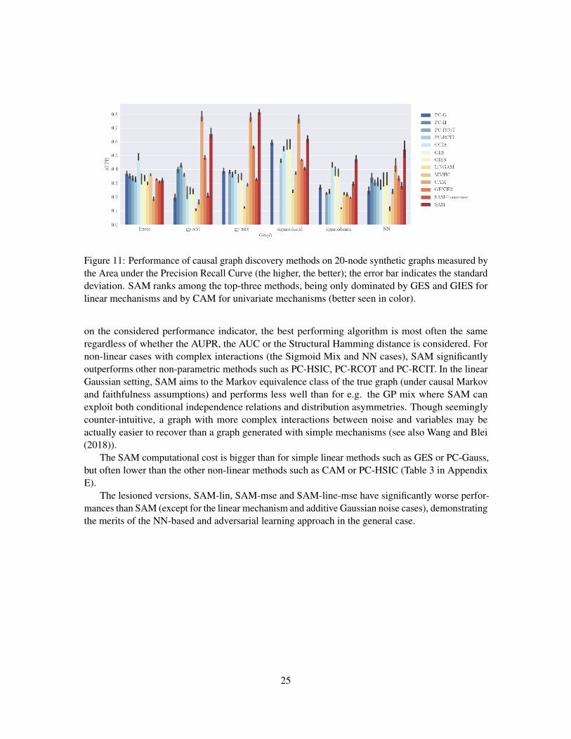
Figure 11: Performance of causal graph discovery methods on 20-node synthetic graphs measured bythe Area under the Precision Recall Curve (the higher, the better); the error bar indicates the standarddeviation. SAM ranks among the top-three methods, being only dominated by GES and GIES forlinear mechanisms and by CAM for univariate mechanisms (better seen in color).

on the considered performance indicator, the best performing algorithm is most often the sameregardless of whether the AUPR, the AUC or the Structural Hamming distance is considered. Fornon-linear cases with complex interactions (the Sigmoid Mix and NN cases), SAM significantlyoutperforms other non-parametric methods such as PC-HSIC, PC-RCOT and PC-RCIT. In the linearGaussian setting, SAM aims to the Markov equivalence class of the true graph (under causal Markovand faithfulness assumptions) and performs less well than for e.g. the GP mix where SAM canexploit both conditional independence relations and distribution asymmetries. Though seeminglycounter-intuitive, a graph with more complex interactions between noise and variables may beactually easier to recover than a graph generated with simple mechanisms (see also Wang and Blei(2018)).

The SAM computational cost is bigger than for simple linear methods such as GES or PC-Gauss,but often lower than the other non-linear methods such as CAM or PC-HSIC (Table 3 in AppendixE).

The lesioned versions, SAM-lin, SAM-mse and SAM-line-mse have significantly worse perfor-mances than SAM (except for the linear mechanism and additive Gaussian noise cases), demonstratingthe merits of the NN-based and adversarial learning approach in the general case.

25

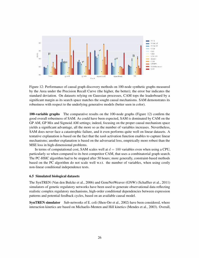
Figure 12: Performance of causal graph discovery methods on 100-node synthetic graphs measuredby the Area under the Precision Recall Curve (the higher, the better); the error bar indicates thestandard deviation. On datasets relying on Gaussian processes, CAM tops the leaderboard by asignificant margin as its search space matches the sought causal mechanisms. SAM demonstrates itsrobustness with respect to the underlying generative models (better seen in color).

100-variable graphs The comparative results on the 100-node graphs (Figure 12) confirm thegood overall robustness of SAM. As could have been expected, SAM is dominated by CAM on theGP AM, GP Mix and Sigmoid AM settings; indeed, focusing on the proper causal mechanism spaceyields a significant advantage, all the more so as the number of variables increases. Nevertheless,SAM does never face a catastrophic failure, and it even performs quite well on linear datasets. Atentative explanation is based on the fact that the tanh activation function enables to capture linearmechanisms; another explanation is based on the adversarial loss, empirically more robust than theMSE loss in high-dimensional problems.

In terms of computational cost, SAM scales well at d = 100 variables even when using a CPU,particularly so when compared to its best competitor CAM, that uses a combinatorial graph search.The PC-HSIC algorithm had to be stopped after 50 hours; more generally, constraint-based methodsbased on the PC algorithm do not scale well w.r.t. the number of variables, when using costlynon-linear conditional independence tests.

6.5 Simulated biological datasets

The SynTREN (Van den Bulcke et al., 2006) and GeneNetWeaver (GNW) (Schaffter et al., 2011)simulators of genetic regulatory networks have been used to generate observational data reflectingrealistic complex regulatory mechanisms, high-order conditional dependencies between expressionpatterns and potential feedback cycles, based on an available causal model.

SynTREN simulator Sub-networks of E. coli (Shen-Orr et al., 2002) have been considered, whereinteraction kinetics are based on Michaelis-Menten and Hill kinetics (Mendes et al., 2003). Overall,

26

20 100Size

0.0

0.1

0.2

0.3

0.4

0.5

0.6

AU

PR

PC-Gauss

PC-HSIC

PC-RCOT

PC-RCIT

GES

GIES

LiNGAM

MMHC

CCDr

CAM

GENIE3

SAM-mse-linear

SAM

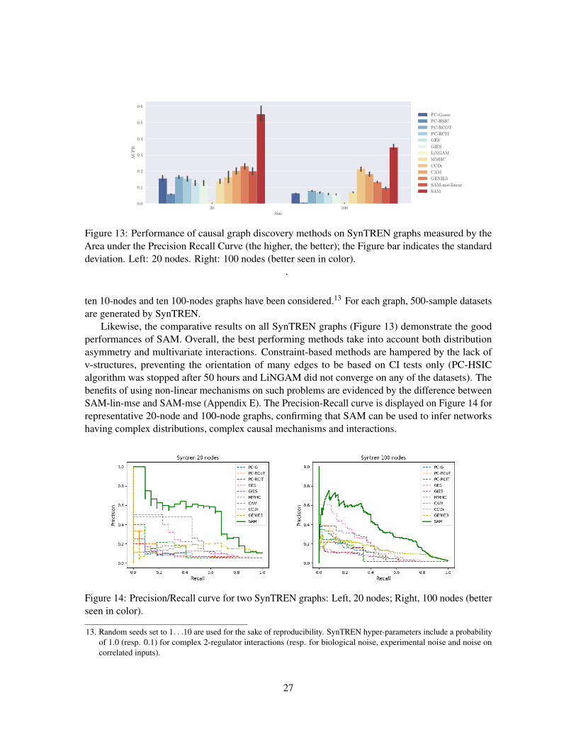
Figure 13: Performance of causal graph discovery methods on SynTREN graphs measured by theArea under the Precision Recall Curve (the higher, the better); the Figure bar indicates the standarddeviation. Left: 20 nodes. Right: 100 nodes (better seen in color).

.

ten 10-nodes and ten 100-nodes graphs have been considered.13 For each graph, 500-sample datasetsare generated by SynTREN.

Likewise, the comparative results on all SynTREN graphs (Figure 13) demonstrate the goodperformances of SAM. Overall, the best performing methods take into account both distributionasymmetry and multivariate interactions. Constraint-based methods are hampered by the lack ofv-structures, preventing the orientation of many edges to be based on CI tests only (PC-HSICalgorithm was stopped after 50 hours and LiNGAM did not converge on any of the datasets). Thebenefits of using non-linear mechanisms on such problems are evidenced by the difference betweenSAM-lin-mse and SAM-mse (Appendix E). The Precision-Recall curve is displayed on Figure 14 forrepresentative 20-node and 100-node graphs, confirming that SAM can be used to infer networkshaving complex distributions, complex causal mechanisms and interactions.

Figure 14: Precision/Recall curve for two SynTREN graphs: Left, 20 nodes; Right, 100 nodes (betterseen in color).

13. Random seeds set to 1. . .10 are used for the sake of reproducibility. SynTREN hyper-parameters include a probabilityof 1.0 (resp. 0.1) for complex 2-regulator interactions (resp. for biological noise, experimental noise and noise oncorrelated inputs).

27

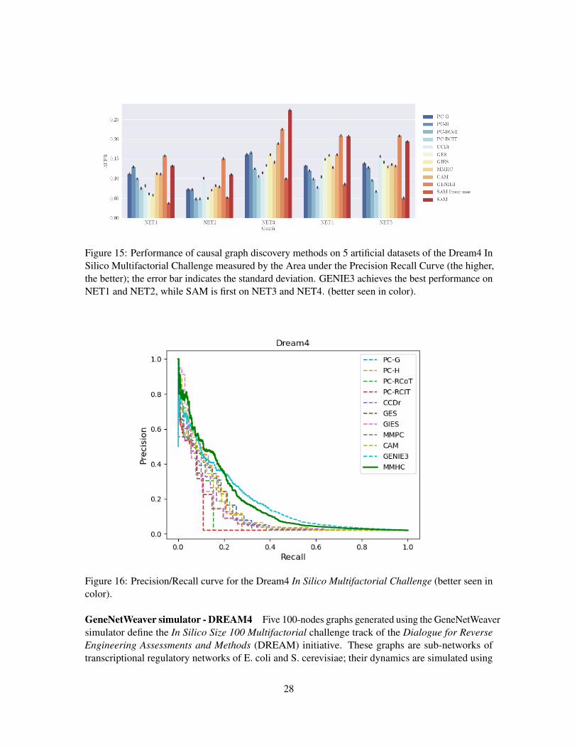
Figure 15: Performance of causal graph discovery methods on 5 artificial datasets of the Dream4 InSilico Multifactorial Challenge measured by the Area under the Precision Recall Curve (the higher,the better); the error bar indicates the standard deviation. GENIE3 achieves the best performance onNET1 and NET2, while SAM is first on NET3 and NET4. (better seen in color).

Figure 16: Precision/Recall curve for the Dream4 In Silico Multifactorial Challenge (better seen incolor).

GeneNetWeaver simulator - DREAM4 Five 100-nodes graphs generated using the GeneNetWeaversimulator define the In Silico Size 100 Multifactorial challenge track of the Dialogue for ReverseEngineering Assessments and Methods (DREAM) initiative. These graphs are sub-networks oftranscriptional regulatory networks of E. coli and S. cerevisiae; their dynamics are simulated using

28

a kinetic gene regulation model, with noise added to both the dynamics of the networks and themeasurement of expression data. Multifactorial perturbations are simulated by slightly increasingor decreasing the basal activation of all genes of the network simultaneously by different randomamounts. In total, the number of expression conditions for each network is set to 100. As theDREAM 4 graphs contain feedback loops, SAM is launched without the DAG constraint on theseinstances.

The comparative results on these five graphs (Figure 15) show that GENIE3 outperforms allother methods on networks 1, 2 and 5, while SAM is better on network 3. The Precision/Recallcurves (Figure 16) show that SAM is slightly better than GENIE3 in the low recall region, but worstin the high recall region. Overall, on such complex problem domains, it seems preferable to makefew assumptions on the underlying generative model (like GENIE3 and SAM), while being able tocapture high-order conditional dependencies between variables. Note that LiNGAM did not convergeon one of these datasets.

GeneNetWeaver simulator - DREAM5 The largest three networks of the DREAM5 challenge(Marbach et al., 2012) are considered to assess the scalability of SAM. Network 1 is a simulatednetwork with simulated expression data (GeneNetWeaver software), while both other expressiondatasets are real expression data collected for E. coli (Network 3) and S. cerevisiae (Network 4).14

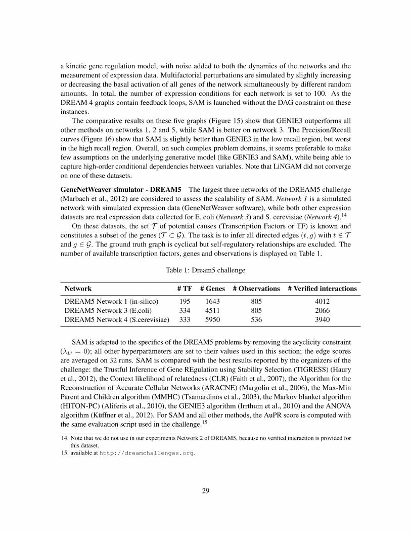
On these datasets, the set T of potential causes (Transcription Factors or TF) is known andconstitutes a subset of the genes (T ⊂ G). The task is to infer all directed edges (t, g) with t ∈ Tand g ∈ G. The ground truth graph is cyclical but self-regulatory relationships are excluded. Thenumber of available transcription factors, genes and observations is displayed on Table 1.

Table 1: Dream5 challenge

Network # TF # Genes # Observations # Verified interactions

DREAM5 Network 1 (in-silico) 195 1643 805 4012DREAM5 Network 3 (E.coli) 334 4511 805 2066DREAM5 Network 4 (S.cerevisiae) 333 5950 536 3940

SAM is adapted to the specifics of the DREAM5 problems by removing the acyclicity constraint(λD = 0); all other hyperparameters are set to their values used in this section; the edge scoresare averaged on 32 runs. SAM is compared with the best results reported by the organizers of thechallenge: the Trustful Inference of Gene REgulation using Stability Selection (TIGRESS) (Hauryet al., 2012), the Context likelihood of relatedness (CLR) (Faith et al., 2007), the Algorithm for theReconstruction of Accurate Cellular Networks (ARACNE) (Margolin et al., 2006), the Max-MinParent and Children algorithm (MMHC) (Tsamardinos et al., 2003), the Markov blanket algorithm(HITON-PC) (Aliferis et al., 2010), the GENIE3 algorithm (Irrthum et al., 2010) and the ANOVAalgorithm (Kuffner et al., 2012). For SAM and all other methods, the AuPR score is computed withthe same evaluation script used in the challenge.15

14. Note that we do not use in our experiments Network 2 of DREAM5, because no verified interaction is provided forthis dataset.

15. available at http://dreamchallenges.org.

29

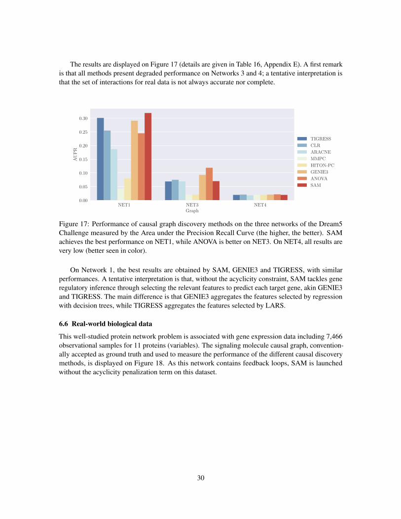
The results are displayed on Figure 17 (details are given in Table 16, Appendix E). A first remarkis that all methods present degraded performance on Networks 3 and 4; a tentative interpretation isthat the set of interactions for real data is not always accurate nor complete.

NET1 NET3 NET4Graph

0.00

0.05

0.10

0.15

0.20

0.25

0.30

AU

PR

TIGRESS

CLR

ARACNE

MMPC

HITON-PC

GENIE3

ANOVA

SAM

Figure 17: Performance of causal graph discovery methods on the three networks of the Dream5Challenge measured by the Area under the Precision Recall Curve (the higher, the better). SAMachieves the best performance on NET1, while ANOVA is better on NET3. On NET4, all results arevery low (better seen in color).

On Network 1, the best results are obtained by SAM, GENIE3 and TIGRESS, with similarperformances. A tentative interpretation is that, without the acyclicity constraint, SAM tackles generegulatory inference through selecting the relevant features to predict each target gene, akin GENIE3and TIGRESS. The main difference is that GENIE3 aggregates the features selected by regressionwith decision trees, while TIGRESS aggregates the features selected by LARS.

6.6 Real-world biological data

This well-studied protein network problem is associated with gene expression data including 7,466observational samples for 11 proteins (variables). The signaling molecule causal graph, convention-ally accepted as ground truth and used to measure the performance of the different causal discoverymethods, is displayed on Figure 18. As this network contains feedback loops, SAM is launchedwithout the acyclicity penalization term on this dataset.

30

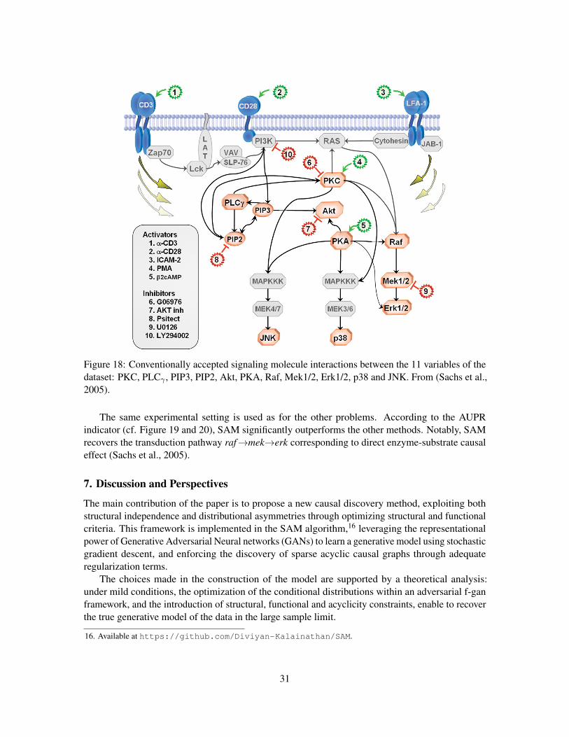
Figure 18: Conventionally accepted signaling molecule interactions between the 11 variables of thedataset: PKC, PLCγ , PIP3, PIP2, Akt, PKA, Raf, Mek1/2, Erk1/2, p38 and JNK. From (Sachs et al.,2005).

The same experimental setting is used as for the other problems. According to the AUPRindicator (cf. Figure 19 and 20), SAM significantly outperforms the other methods. Notably, SAMrecovers the transduction pathway raf→mek→erk corresponding to direct enzyme-substrate causaleffect (Sachs et al., 2005).

7. Discussion and Perspectives

The main contribution of the paper is to propose a new causal discovery method, exploiting bothstructural independence and distributional asymmetries through optimizing structural and functionalcriteria. This framework is implemented in the SAM algorithm,16 leveraging the representationalpower of Generative Adversarial Neural networks (GANs) to learn a generative model using stochasticgradient descent, and enforcing the discovery of sparse acyclic causal graphs through adequateregularization terms.

The choices made in the construction of the model are supported by a theoretical analysis:under mild conditions, the optimization of the conditional distributions within an adversarial f-ganframework, and the introduction of structural, functional and acyclicity constraints, enable to recoverthe true generative model of the data in the large sample limit.

16. Available at https://github.com/Diviyan-Kalainathan/SAM.

31

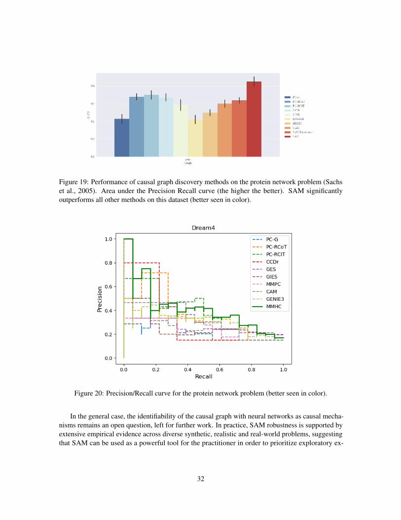
Figure 19: Performance of causal graph discovery methods on the protein network problem (Sachset al., 2005). Area under the Precision Recall curve (the higher the better). SAM significantlyoutperforms all other methods on this dataset (better seen in color).

Figure 20: Precision/Recall curve for the protein network problem (better seen in color).

In the general case, the identifiability of the causal graph with neural networks as causal mecha-nisms remains an open question, left for further work. In practice, SAM robustness is supported byextensive empirical evidence across diverse synthetic, realistic and real-world problems, suggestingthat SAM can be used as a powerful tool for the practitioner in order to prioritize exploratory ex-

32

periments when working on real data with no prior information about neither the type of functionalmechanisms involved, nor the underlying data distribution.

Lesion studies are conducted to assess whether and when it is beneficial to learn non-linearmechanisms and to rely on adversarial learning as opposed to MSE minimization.As could have been expected, in particular settings SAM is dominated by algorithms specificallydesigned for these settings, such as CAM (Buhlmann et al., 2014) in the case of additive noise modeland Gaussian process mechanisms, and GENIE3 when facing causal graphs with feedback loops forsome networks. Nevertheless, SAM most often ranks first and always avoids catastrophic failures.SAM has good overall computational efficiency compared to other non-linear methods as it usesan embedded framework for structure optimization, where the mechanisms and the structure aresimultaneously learned within an end-to-end DAG learning framework. It can also easily be trainedon a GPU device, thus leveraging on massive parallel computation power available to learn the DAGmechanisms and the adversarial neural network. SAM scalability is demonstrated on the Network1 of the DREAM5 challenge, obtaining very good performances with a relatively high number ofvariables (ca 1,500).

This work opens up four avenues for further research. An on-going extension regards the caseof categorical and mixed variables, taking inspiration from discrete GANs (Hjelm et al., 2017).Another perspective is to relax the causal sufficiency assumption and handle hidden confounders, e.g.by introducing statistical dependencies between the noise variables attached to different variables(Rothenhausler et al., 2015), or creating shared noise variables (Janzing and Scholkopf, 2018), orvia dimensionality reduction (Wang and Blei, 2018). A longer term perspective is to extend SAMto simulate interventions on target variables. Lastly, the case of causal graphs with cycles will beconsidered, leveraging the power of recurrent neural nets to define a proper generative model from agraph with feedback loops.

Acknowledgment

We would like to thank Dr. Mikael Escobar-Bach for proofreading the paper. This work was grantedaccess to the HPC resources of CCIPL (Nantes, France).

References

Constantin F Aliferis, Ioannis Tsamardinos, and Alexander Statnikov. Hiton: a novel Markov blanketalgorithm for optimal variable selection. In AMIA annual symposium proceedings, volume 2003,page 21. American Medical Informatics Association, 2003.

Constantin F Aliferis, Alexander Statnikov, Ioannis Tsamardinos, Subramani Mani, and Xenofon DKoutsoukos. Local causal and Markov blanket induction for causal discovery and feature selectionfor classification part I: Algorithms and empirical evaluation. Journal of Machine LearningResearch, 11(1), 2010.

Bryon Aragam and Qing Zhou. Concave penalized estimation of sparse gaussian bayesian networks.Journal of Machine Learning Research, 16:2273–2328, 2015.

Bryon Aragam, Jiaying Gu, and Qing Zhou. Learning large-scale bayesian networks with thesparsebn package. arXiv preprint arXiv:1703.04025, 2017.

33

David A Bell and Hui Wang. A formalism for relevance and its application in feature subset selection.Machine learning, 41(2):175–195, 2000.

Patrick Blobaum, Dominik Janzing, Takashi Washio, Shohei Shimizu, and Bernhard Scholkopf.Cause-effect inference by comparing regression errors. In International Conference on ArtificialIntelligence and Statistics, pages 900–909. PMLR, 2018.

Gavin Brown, Adam Pocock, Ming-Jie Zhao, and Mikel Lujan. Conditional likelihood maximisation:a unifying framework for information theoretic feature selection. Journal of machine learningresearch, 13(Jan):27–66, 2012.

Peter Buhlmann, Jonas Peters, Jan Ernest, et al. Cam: Causal additive models, high-dimensionalorder search and penalized regression. The Annals of Statistics, 42(6):2526–2556, 2014.

Pu Chen, Chihying Hsiao, Peter Flaschel, and Willi Semmler. Causal analysis in economics: Methodsand applications. 2007.

David Maxwell Chickering. Optimal structure identification with greedy search. Journal of MachineLearning Research, 2002.

David Maxwell Chickering. A transformational characterization of equivalent bayesian networkstructures. arXiv preprint arXiv:1302.4938, 2013.

Diego Colombo and Marloes H Maathuis. Order-independent constraint-based causal structurelearning. Journal of Machine Learning Research, 2014.

Diego Colombo, Marloes H Maathuis, Markus Kalisch, and Thomas S Richardson. Learning high-dimensional directed acyclic graphs with latent and selection variables. The Annals of Statistics,2012.

Povilas Daniusis, Dominik Janzing, Joris Mooij, Jakob Zscheischler, Bastian Steudel, Kun Zhang,and Bernhard Scholkopf. Inferring deterministic causal relations. arXiv, 2012.

F. Doshi-Velez and B. Kim. Towards a rigorous science of interpretable machine learning.arXiv:1702.08608, 2017.

Jeremiah J Faith, Boris Hayete, Joshua T Thaden, Ilaria Mogno, Jamey Wierzbowski, GuillaumeCottarel, Simon Kasif, James J Collins, and Timothy S Gardner. Large-scale mapping andvalidation of escherichia coli transcriptional regulation from a compendium of expression profiles.PLoS biol, 5(1):e8, 2007.

Nir Friedman and Iftach Nachman. Gaussian process networks. In Proceedings of the SixteenthConference on Uncertainty in Artificial Intelligence, UAI’00, page 211–219, San Francisco, CA,USA, 2000. Morgan Kaufmann Publishers Inc. ISBN 1558607099.

Ian Goodfellow, Jean Pouget-Abadie, Mehdi Mirza, Bing Xu, David Warde-Farley, Sherjil Ozair,Aaron Courville, and Yoshua Bengio. Generative adversarial nets. Advances in Neural InformationProcessing Systems, 2014.

34

Olivier Goudet, Diviyan Kalainathan, Philippe Caillou, Isabelle Guyon, David Lopez-Paz, andMichele Sebag. Learning functional causal models with generative neural networks. In Explainableand Interpretable Models in Computer Vision and Machine Learning, pages 39–80. Springer,2018.

Arthur Gretton, Ralf Herbrich, Alexander Smola, Olivier Bousquet, and Bernhard Scholkopf. Kernelmethods for measuring independence. Journal of Machine Learning Research, 2005.

Arthur Gretton, Karsten M Borgwardt, Malte Rasch, Bernhard Scholkopf, Alexander J Smola, et al. Akernel method for the two-sample-problem. Advances in Neural Information Processing Systems,2007.

Isabelle Guyon, Alexander Statnikov, and Berna Bakir Batu. Cause Effect Pairs in Machine Learning.Springer International Publishing, 2019. ISBN 978-3-030-21809-6.

Anne-Claire Haury, Fantine Mordelet, Paola Vera-Licona, and Jean-Philippe Vert. Tigress: trustfulinference of gene regulation using stability selection. BMC systems biology, 6(1):145, 2012.

Alain Hauser and Peter Buhlmann. Characterization and greedy learning of interventional Markovequivalence classes of directed acyclic graphs. Journal of Machine Learning Research, 13(Aug):2409–2464, 2012.

R Devon Hjelm, Athul Paul Jacob, Tong Che, Adam Trischler, Kyunghyun Cho, and Yoshua Bengio.Boundary-seeking generative adversarial networks. arXiv preprint arXiv:1702.08431, 2017.

Patrik O Hoyer, Dominik Janzing, Joris M Mooij, Jonas Peters, and Bernhard Scholkopf. Nonlinearcausal discovery with additive noise models. Advances in Neural Information Processing Systems,2009.

Aapo Hyvarinen and Petteri Pajunen. Nonlinear independent component analysis: Existence anduniqueness results. Neural Networks, 12(3):429–439, 1999.

Guido W Imbens and Donald B Rubin. Causal inference in statistics, social, and biomedical sciences.Cambridge University Press, 2015.

Sergey Ioffe and Christian Szegedy. Batch normalization: Accelerating deep network training byreducing internal covariate shift. In International conference on machine learning, pages 448–456,2015.

Alexandre Irrthum, Louis Wehenkel, Pierre Geurts, et al. Inferring regulatory networks fromexpression data using tree-based methods. PloS one, 5(9):e12776, 2010.

Eric Jang, Shixiang Gu, and Ben Poole. Categorical reparameterization with gumbel-softmax. arXivpreprint arXiv:1611.01144, 2016.

Dominik Janzing and Bernhard Scholkopf. Detecting confounding in multivariate linear models viaspectral analysis. Journal of Causal Inference, 6(1), 2018.

Markus Kalisch and Peter Buhlmann. Estimating high-dimensional directed acyclic graphs with thepc-algorithm. Journal of Machine Learning Research, 8(Mar):613–636, 2007.

35

Markus Kalisch, Martin Machler, Diego Colombo, Marloes H Maathuis, Peter Buhlmann, et al.Causal inference using graphical models with the R package pcalg. Journal of Statistical Software,2012.

Tero Karras, Timo Aila, Samuli Laine, and Jaakko Lehtinen. Progressive growing of GANs forimproved quality, stability, and variation. arXiv preprint arXiv:1710.10196, 2017.

Durk P Kingma and Jimmy Ba. Adam: A Method for Stochastic Optimization. Int. Conf. on LearningRepresentations, 2014.

Robert Kuffner, Tobias Petri, Pegah Tavakkolkhah, Lukas Windhager, and Ralf Zimmer. Inferringgene regulatory networks by anova. Bioinformatics, 28(10):1376–1382, 2012.

Philippe Leray and Patrick Gallinari. Feature selection with neural networks. Behaviormetrika, 26(1):145–166, 1999.

David Lopez-Paz and Maxime Oquab. Revisiting classifier two-sample tests. arXiv preprintarXiv:1610.06545, 2016.

David Lopez-Paz, Krikamol Muandet, Bernhard Scholkopf, and Ilya O Tolstikhin. Towards a learningtheory of cause-effect inference. Int. Conf. on Machine Learning, 2015.

Christos Louizos, Max Welling, and Diederik P Kingma. Learning sparse neural networks throughl 0 regularization. arXiv preprint arXiv:1712.01312, 2017.

Chris J Maddison, Andriy Mnih, and Yee Whye Teh. The concrete distribution: A continuousrelaxation of discrete random variables. arXiv preprint arXiv:1611.00712, 2016.

Daniel Marbach, Thomas Schaffter, Dario Floreano, Robert J Prill, and Gustavo Stolovitzky. Thedream4 in-silico network challenge. Draft, version 0.3, 2009.

Daniel Marbach, James C Costello, Robert Kuffner, Nicole M Vega, Robert J Prill, Diogo MCamacho, Kyle R Allison, Manolis Kellis, James J Collins, and Gustavo Stolovitzky. Wisdom ofcrowds for robust gene network inference. Nature methods, 9(8):796–804, 2012.

Adam A Margolin, Ilya Nemenman, Katia Basso, Chris Wiggins, Gustavo Stolovitzky, RiccardoDalla Favera, and Andrea Califano. Aracne: an algorithm for the reconstruction of gene regulatorynetworks in a mammalian cellular context. In BMC bioinformatics, volume 7, page S7. Springer,2006.

Pedro Mendes, Wei Sha, and Keying Ye. Artificial gene networks for objective comparison ofanalysis algorithms. Bioinformatics, 19(suppl 2):ii122–ii129, 2003.

Mehdi Mirza and Simon Osindero. Conditional generative adversarial nets. arXiv, 2014.

Joris M Mooij, Oliver Stegle, Dominik Janzing, Kun Zhang, , and Bernhard Scholkopf. Probabilisticlatent variable models for distinguishing between cause and effect. Advances in Neural InformationProcessing Systems, 2010.

36

Joris M Mooij, Jonas Peters, Dominik Janzing, Jakob Zscheischler, and Bernhard Scholkopf. Dis-tinguishing cause from effect using observational data: methods and benchmarks. Journal ofMachine Learning Research, 2016.

Preetam Nandy, Alain Hauser, and Marloes H Maathuis. High-dimensional consistency in score-based and hybrid structure learning. arXiv, 2015.

Behnam Neyshabur, Srinadh Bhojanapalli, David McAllester, and Nati Srebro. Exploring generaliza-tion in deep learning. In Advances in Neural Information Processing Systems, pages 5947–5956,2017.

XuanLong Nguyen, Martin J Wainwright, and Michael I Jordan. Estimating divergence functionalsand the likelihood ratio by convex risk minimization. IEEE Transactions on Information Theory,56(11):5847–5861, 2010.

Sebastian Nowozin, Botond Cseke, and Ryota Tomioka. f-gan: Training generative neural samplersusing variational divergence minimization. In Advances in Neural Information Processing Systems,pages 271–279, 2016.

Juan Miguel Ogarrio, Peter Spirtes, and Joe Ramsey. A hybrid causal search algorithm for latentvariable models. Conference on Probabilistic Graphical Models, 2016.

Judea Pearl. Causality: models, reasoning, and inference. Econometric Theory, 19(675-685):46,2003.

Judea Pearl. Causality. 2009.

Judea Pearl and Thomas Verma. A formal theory of inductive causation. 1991.

F. Pedregosa, G. Varoquaux, A. Gramfort, V. Michel, B. Thirion, O. Grisel, M. Blondel, P. Pretten-hofer, R. Weiss, V. Dubourg, J. Vanderplas, A. Passos, D. Cournapeau, M. Brucher, M. Perrot, andE. Duchesnay. Scikit-learn: Machine learning in Python. Journal of Machine Learning Research,12:2825–2830, 2011.

Jonas Peters, Joris M Mooij, Dominik Janzing, and Bernhard Scholkopf. Causal discovery withcontinuous additive noise models. The Journal of Machine Learning Research, 15(1):2009–2053,2014.

Jonas Peters, Dominik Janzing, and Bernhard Scholkopf. Elements of Causal Inference - Foundationsand Learning Algorithms. MIT Press, 2017.

John A Quinn, Joris M Mooij, Tom Heskes, and Michael Biehl. Learning of causal relations. ESANN,2011.

Joseph Ramsey, Madelyn Glymour, Ruben Sanchez-Romero, and Clark Glymour. A million variablesand more: the fast greedy equivalence search algorithm for learning high-dimensional graphicalcausal models, with an application to functional magnetic resonance images. International journalof data science and analytics, 3(2):121–129, 2017.

Joseph D Ramsey. Scaling up greedy causal search for continuous variables. arXiv, 2015.

37

Dominik Rothenhausler, Christina Heinze, Jonas Peters, and Nicolai Meinshausen. Backshift:Learning causal cyclic graphs from unknown shift interventions. In Advances in Neural InformationProcessing Systems, pages 1513–1521, 2015.

Karen Sachs, Omar Perez, Dana Pe’er, Douglas A Lauffenburger, and Garry P Nolan. Causalprotein-signaling networks derived from multiparameter single-cell data. Science, 308(5721):523–529, 2005.

Thomas Schaffter, Daniel Marbach, and Dario Floreano. Genenetweaver: in silico benchmarkgeneration and performance profiling of network inference methods. Bioinformatics, 27(16):2263–2270, 2011.

Marco Scutari. Learning bayesian networks with the bnlearn r package. arXiv, 2009.

Shai S Shen-Orr, Ron Milo, Shmoolik Mangan, and Uri Alon. Network motifs in the transcriptionalregulation network of escherichia coli. Nature genetics, 31(1):64, 2002.

Shohei Shimizu, Patrik O Hoyer, Aapo Hyvarinen, and Antti Kerminen. A linear non-gaussianacyclic model for causal discovery. Journal of Machine Learning Research, 2006.

Peter Spirtes and Kun Zhang. Causal discovery and inference: concepts and recent methodologicaladvances. Applied informatics, 2016.

Peter Spirtes, Clark Glymour, and Richard Scheines. Causation, prediction and search. 1993. LectureNotes in Statistics, 1993.

Peter Spirtes, Clark N Glymour, and Richard Scheines. Causation, prediction, and search. 2000.

Nitish Srivastava, Geoffrey Hinton, Alex Krizhevsky, Ilya Sutskever, and Ruslan Salakhutdinov.Dropout: a simple way to prevent neural networks from overfitting. The Journal of MachineLearning Research, 15(1):1929–1958, 2014.

Alexander Statnikov, Mikael Henaff, Nikita I Lytkin, and Constantin F Aliferis. New methods forseparating causes from effects in genomics data. BMC genomics, 2012.

Eric V Strobl, Kun Zhang, and Shyam Visweswaran. Approximate kernel-based conditional in-dependence tests for fast non-parametric causal discovery. arXiv preprint arXiv:1702.03877,2017.

Ioannis Tsamardinos, Constantin F. Aliferis, and Alexander Statnikov. Time and sample efficientdiscovery of Markov blankets and direct causal relations. In Proceedings of the ninth ACMSIGKDD international conference on Knowledge discovery and data mining, pages 673–678,2003.

Ioannis Tsamardinos, Laura E Brown, and Constantin F Aliferis. The max-min hill-climbing bayesiannetwork structure learning algorithm. Machine learning, 65(1):31–78, 2006.

Tim Van den Bulcke, Koenraad Van Leemput, Bart Naudts, Piet van Remortel, Hongwu Ma, AlainVerschoren, Bart De Moor, and Kathleen Marchal. Syntren: a generator of synthetic geneexpression data for design and analysis of structure learning algorithms. BMC bioinformatics, 7(1):43, 2006.

38

Jorge R. Vergara and Pablo A. Estevez. A review of feature selection methods based on mutualinformation. Neural computing and applications, 24(1):175–186, 2014.

Yixin Wang and David M. Blei. The blessings of multiple causes. CoRR, abs/1805.06826, 2018.URL http://arxiv.org/abs/1805.06826.

Kui Yu, Lin Liu, and Jiuyong Li. A unified view of causal and non-causal feature selection. arXivpreprint arXiv:1802.05844, 2018.

Kun Zhang and Aapo Hyvarinen. Distinguishing causes from effects using nonlinear acyclic causalmodels. In Causality: Objectives and Assessment, pages 157–164, 2010.

Kun Zhang, Jonas Peters, Dominik Janzing, and Bernhard Scholkopf. Kernel-based conditionalindependence test and application in causal discovery. arXiv, 2012.

Xun Zheng, Bryon Aragam, Pradeep Ravikumar, and Eric P. Xing. Dags with NO TEARS: continuousoptimization for structure learning. In Advances in Neural Information Processing Systems(NeurIPS), pages 9492–9503, 2018.

39

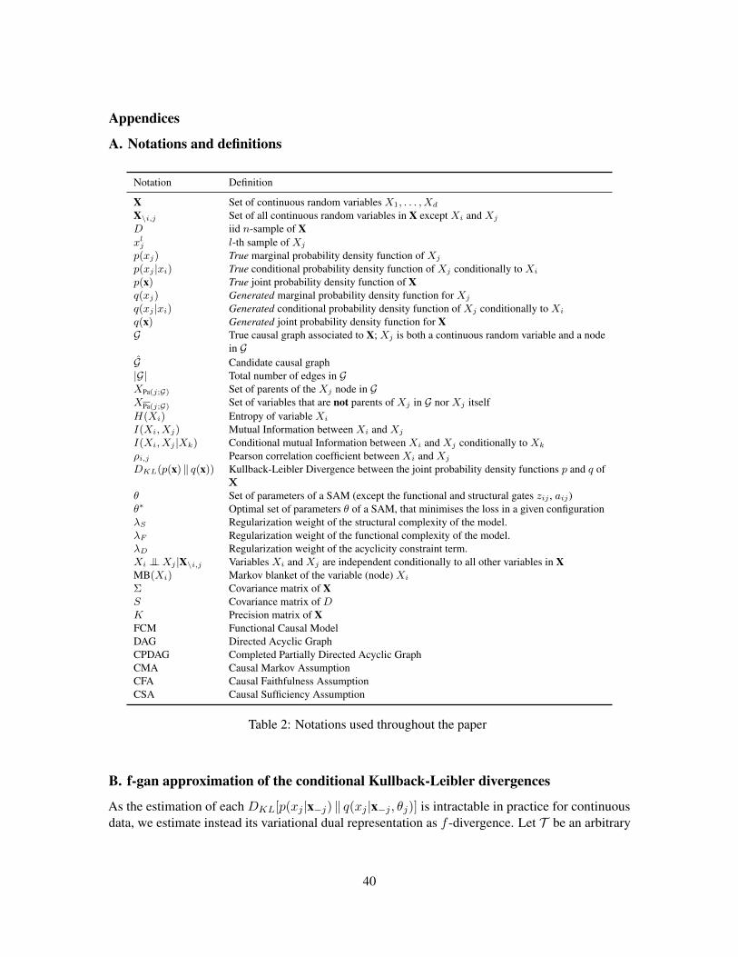
Appendices

A. Notations and definitions

Notation Definition

X Set of continuous random variables X1, . . . , Xd

X\i,j Set of all continuous random variables in X except Xi and Xj

D iid n-sample of Xxlj l-th sample of Xj

p(xj) True marginal probability density function of Xj

p(xj |xi) True conditional probability density function of Xj conditionally to Xi

p(x) True joint probability density function of Xq(xj) Generated marginal probability density function for Xj

q(xj |xi) Generated conditional probability density function of Xj conditionally to Xi

q(x) Generated joint probability density function for XG True causal graph associated to X; Xj is both a continuous random variable and a node

in GG Candidate causal graph|G| Total number of edges in GXPa(j;G) Set of parents of the Xj node in GXPa(j;G) Set of variables that are not parents of Xj in G nor Xj itselfH(Xi) Entropy of variable Xi

I(Xi, Xj) Mutual Information between Xi and Xj

I(Xi, Xj |Xk) Conditional mutual Information between Xi and Xj conditionally to Xk

ρi,j Pearson correlation coefficient between Xi and Xj

DKL(p(x) ‖ q(x)) Kullback-Leibler Divergence between the joint probability density functions p and q ofX

θ Set of parameters of a SAM (except the functional and structural gates zij , aij)θ∗ Optimal set of parameters θ of a SAM, that minimises the loss in a given configurationλS Regularization weight of the structural complexity of the model.λF Regularization weight of the functional complexity of the model.λD Regularization weight of the acyclicity constraint term.Xi ⊥⊥Xj |X\i,j Variables Xi and Xj are independent conditionally to all other variables in XMB(Xi) Markov blanket of the variable (node) Xi

Σ Covariance matrix of XS Covariance matrix of DK Precision matrix of XFCM Functional Causal ModelDAG Directed Acyclic GraphCPDAG Completed Partially Directed Acyclic GraphCMA Causal Markov AssumptionCFA Causal Faithfulness AssumptionCSA Causal Sufficiency Assumption

Table 2: Notations used throughout the paper

B. f-gan approximation of the conditional Kullback-Leibler divergences

As the estimation of each DKL[p(xj |x−j) ‖ q(xj |x−j , θj)] is intractable in practice for continuousdata, we estimate instead its variational dual representation as f -divergence. Let T be an arbitrary

40

class of functions T : Rd → R. For two distributions p and q defined over Rd, Nguyen et al. (2010)establish the following lower bound (tight for sufficiently large families T ):

DKL[p ‖ q] ≥ supT∈T

Ex∼p(x)[T (x)]− Ex∼q(x)[eT (x)−1], (22)

The f-gan approach proposed by Nowozin et al. (2016) consists of defining T as the family offunctions Tω : Rd → R parameterized by a deep neural network with parameter ω ∈ Ω. This familysupports the following estimation of DKL[p ‖ q]:

DΩKL[p ‖ q] = sup

ω∈ΩEx∼p(x)[Tω(x)]− Ex∼q(x)[e

Tω(x)−1], (23)

SAM relies on the f-gan loss to train the d neural networks generator fj , as follows. For` = 1, . . . , n, let x(`)

−j be defined from x(`) by taking all its coordinates but the j-th, let e(`)j be drawn

from N (0, 1), and let scalar x(`)j be computed from fj (Equation (3)) as:

x(`)j = fj(x(`)

−j , e(`)j )

Let the pseudo-sample x(`)j be defined from x(`) by setting its j-th coordinate to x(`)

j , and let the

dataset Dj include all pseudo-samples x(`)j for ` = 1 . . . n. For j = 1, . . . , d, let T jω be trained to

discriminate between the original dataset D and dataset Dj . Accordingly:

DΩj

KL[p(xj , x−j) ‖ q(xj , x−j , θj)] = supω∈Ωj

limn→∞

(1

n

n∑`=1

T jω(x(`))

+1

n

n∑`=1

[− exp(T jω(xj(`))− 1) ]

)(24)

SAM proceeds by finding a shared discriminator Tω with parameter ω ∈ Ω that simultaneouslymaximizes all expressions 1

n

∑n`=1 T

jω(x(`)) + 1

n

∑n`=1[− exp(T jω(xj(`)) − 1) ] for j ∈ J1, dK and

such that:

d∑j=1

DΩKL[p(xj , x−j) ‖ q(xj , x−j , θj)] = sup

ω∈Ωlimn→∞

1

n

d∑j=1

(n∑`=1

Tω(x(`)) +

n∑`=1

[− exp(Tω(xj(`))− 1)]

)(25)

Using a shared discriminator Tω to achieve the d discrimination tasks is not only more compu-tationally efficient; it also improves the stability of the algorithm, avoiding the gradient vanishingphenomena that were empirically observed when solving separately the d min-max optimizationproblems with d different discriminators.

Furthermore, by construction as p(xj , x−j) = p(x−j)p(xj |x−j), andq(xj , x−j , θj) = p(x−j)q(xj |x−j , θj), we have:

DKL[p(xj , x−j) ‖ q(xj , x−j , θj)] = DKL[p(xj |x−j) ‖ q(xj |x−j , θj)] (26)

41

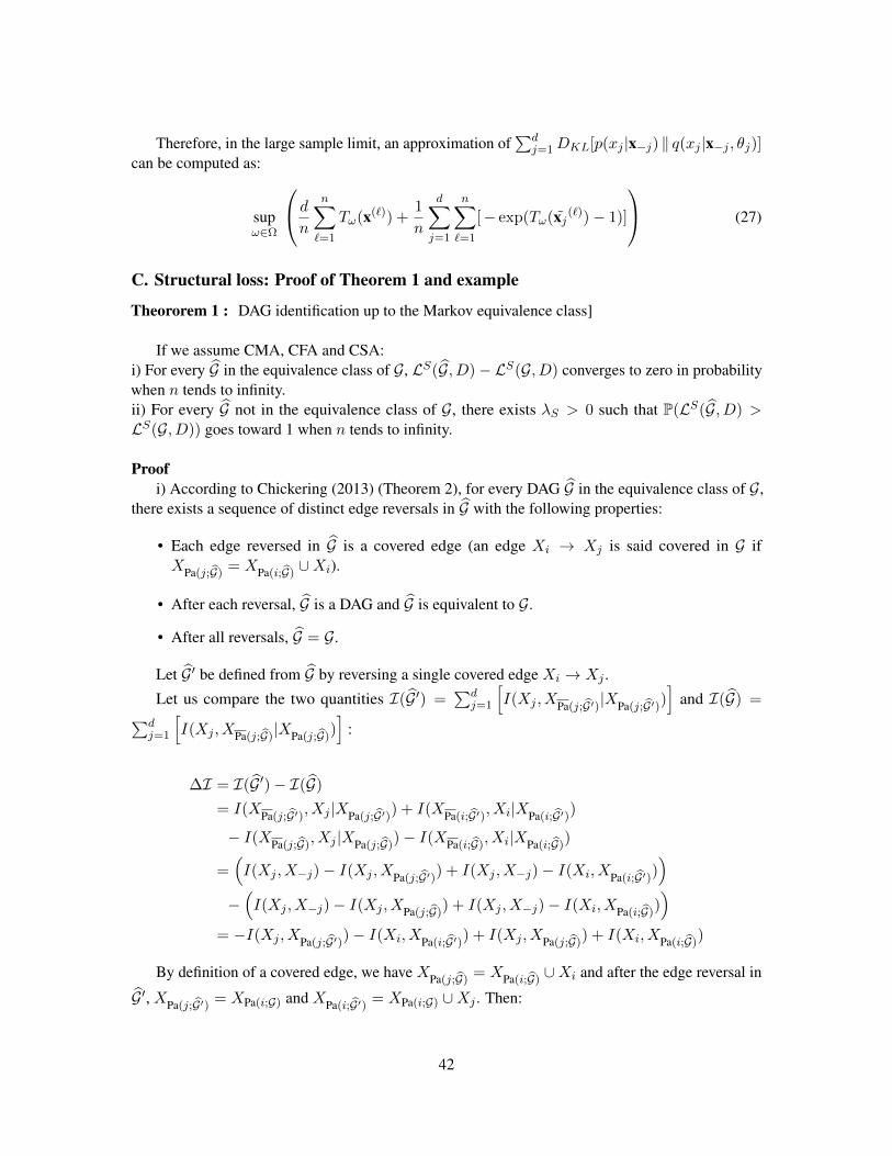
Therefore, in the large sample limit, an approximation of∑d

j=1DKL[p(xj |x−j) ‖ q(xj |x−j , θj)]can be computed as:

supω∈Ω

d

n

n∑`=1

Tω(x(`)) +1

n

d∑j=1

n∑`=1

[− exp(Tω(xj(`))− 1)]

(27)

C. Structural loss: Proof of Theorem 1 and example

Theororem 1 : DAG identification up to the Markov equivalence class]

If we assume CMA, CFA and CSA:i) For every G in the equivalence class of G, LS(G, D)− LS(G, D) converges to zero in probabilitywhen n tends to infinity.ii) For every G not in the equivalence class of G, there exists λS > 0 such that P(LS(G, D) >LS(G, D)) goes toward 1 when n tends to infinity.

Proofi) According to Chickering (2013) (Theorem 2), for every DAG G in the equivalence class of G,

there exists a sequence of distinct edge reversals in G with the following properties:

• Each edge reversed in G is a covered edge (an edge Xi → Xj is said covered in G ifXPa(j;G)

= XPa(i;G)∪Xi).

• After each reversal, G is a DAG and G is equivalent to G.

• After all reversals, G = G.

Let G′ be defined from G by reversing a single covered edge Xi → Xj .

Let us compare the two quantities I(G′) =∑d

j=1

[I(Xj , XPa(j;G′)|XPa(j;G′))

]and I(G) =∑d

j=1

[I(Xj , XPa(j;G)

|XPa(j;G))]

:

∆I = I(G′)− I(G)

= I(XPa(j;G′), Xj |XPa(j;G′)) + I(XPa(i;G′), Xi|XPa(i;G′))

− I(XPa(j;G), Xj |XPa(j;G)

)− I(XPa(i;G), Xi|XPa(i;G)

)

=(I(Xj , X−j)− I(Xj , XPa(j;G′)) + I(Xj , X−j)− I(Xi, XPa(i;G′))

)−(I(Xj , X−j)− I(Xj , XPa(j;G)

) + I(Xj , X−j)− I(Xi, XPa(i;G)))

= −I(Xj , XPa(j;G′))− I(Xi, XPa(i;G′)) + I(Xj , XPa(j;G)) + I(Xi, XPa(i;G)

)

By definition of a covered edge, we have XPa(j;G)= XPa(i;G)

∪Xi and after the edge reversal in

G′, XPa(j;G′) = XPa(i;G) and XPa(i;G′) = XPa(i;G) ∪Xj . Then:

42

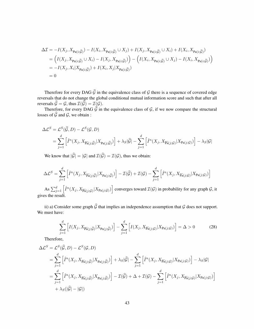
∆I = −I(Xj , XPa(i;G))− I(Xi, XPa(i;G)

∪Xj) + I(Xj , XPa(i;G)∪Xi) + I(Xi, XPa(i;G)

)

=(I(Xj , XPa(i;G)

∪Xi)− I(Xj , XPa(i;G)))−(I(Xi, XPa(i;G)

∪Xj)− I(Xi, XPa(i;G)))

= −I(Xj , Xi|XPa(i;G)) + I(Xi, Xj |XPa(i;G)

)

= 0

Therefore for every DAG G in the equivalence class of G there is a sequence of covered edgereversals that do not change the global conditional mutual information score and such that after allreversals G = G, thus I(G) = I(G).

Therefore, for every DAG G in the equivalence class of G, if we now compare the structurallosses of G and G, we obtain :

∆LS = LS(G, D)− LS(G, D)

=d∑j=1

[In(Xj , XPa(j;G)

|XPa(j;G))]

+ λS |G| −d∑j=1

[In(Xj , XPa(j;G)|XPa(j;G))

]− λS |G|

We know that |G| = |G| and I(G) = I(G), thus we obtain:

∆LS =d∑j=1

[In(Xj , XPa(j;G)

|XPa(j;G))]− I(G) + I(G)−

d∑j=1

[In(Xj , XPa(j;G)|XPa(j;G))

]As∑d

j=1

[In(Xj , XPa(j;G)|XPa(j;G))

]converges toward I(G) in probability for any graph G, it

gives the result.

ii) a) Consider some graph G that implies an independence assumption that G does not support.We must have:

d∑j=1

[I(Xj , XPa(j;G)

|XPa(j;G))]−

d∑j=1

[I(Xj , XPa(j;G)|XPa(j;G))

]= ∆ > 0 (28)

Therefore,

∆LS = LS(G, D)− LS(G, D)

=

d∑j=1

[In(Xj , XPa(j;G)

|XPa(j;G))]

+ λS |G| −d∑j=1

[In(Xj , XPa(j;G)|XPa(j;G))

]− λS |G|

=

d∑j=1

[In(Xj , XPa(j;G)

|XPa(j;G))]− I(G) + ∆ + I(G)−

d∑j=1

[In(Xj , XPa(j;G)|XPa(j;G))

]+ λS(|G| − |G|)

43

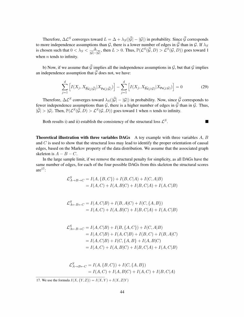
Therefore, ∆LS converges toward L = ∆ + λS(|G| − |G|) in probability. Since G correspondsto more independence assumptions than G, there is a lower number of edges in G than in G. If λSis chosen such that 0 < λS <

∆

|G|−|G|, then L > 0. Thus, P(LS(G, D) > LS(G, D)) goes toward 1

when n tends to infinity.

b) Now, if we assume that G implies all the independence assumptions in G, but that G impliesan independence assumption that G does not, we have:

d∑j=1

[I(Xj , XPa(j;G)

|XPa(j;G))]−

d∑j=1

[I(Xj , XPa(j;G)|XPa(j;G))

]= 0 (29)

Therefore, ∆LS converges toward λS(|G| − |G|) in probability. Now, since G corresponds tofewer independence assumptions than G, there is a higher number of edges in G than in G. Thus,|G| > |G|. Then, P(LS(G, D) > LS(G, D)) goes toward 1 when n tends to infinity.

Both results i) and ii) establish the consistency of the structural loss LS .

Theoretical illustration with three variables DAGs A toy example with three variables A, Band C is used to show that the structural loss may lead to identify the proper orientation of causaledges, based on the Markov property of the data distribution. We assume that the associated graphskeleton is A−B − C.

In the large sample limit, if we remove the structural penalty for simplicity, as all DAGs have thesame number of edges, for each of the four possible DAGs from this skeleton the structural scoresare17:

LSA→B→C = I(A, B,C) + I(B,C|A) + I(C,A|B)

= I(A,C) + I(A,B|C) + I(B,C|A) + I(A,C|B)

LSA←B←C = I(A,C|B) + I(B,A|C) + I(C, A,B)= I(A,C) + I(A,B|C) + I(B,C|A) + I(A,C|B)

LSA←B→C = I(A,C|B) + I(B, A,C) + I(C,A|B)

= I(A,C|B) + I(A,C|B) + I(B,C) + I(B,A|C)

= I(A,C|B) + I(C, A,B+ I(A,B|C)

= I(A,C) + I(A,B|C) + I(B,C|A) + I(A,C|B)

LSA→B←C = I(A, B,C) + I(C, A,B)= I(A,C) + I(A,B|C) + I(A,C) + I(B,C|A)

17. We use the formula I(X, Y,Z) = I(X,Y ) + I(X,Z|Y )

44

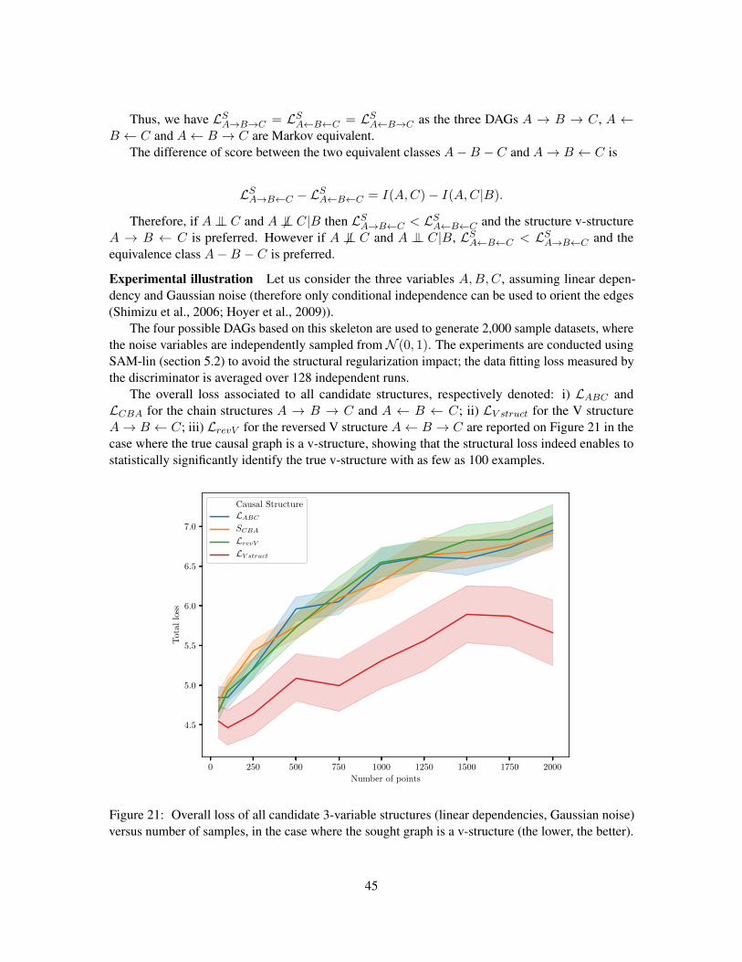
Thus, we have LSA→B→C = LSA←B←C = LSA←B→C as the three DAGs A → B → C, A ←B ← C and A← B → C are Markov equivalent.

The difference of score between the two equivalent classes A−B − C and A→ B ← C is

LSA→B←C − LSA←B←C = I(A,C)− I(A,C|B).

Therefore, if A⊥⊥ C and A⊥6⊥ C|B then LSA→B←C < LSA←B←C and the structure v-structureA → B ← C is preferred. However if A ⊥6⊥ C and A ⊥⊥ C|B, LSA←B←C < LSA→B←C and theequivalence class A−B − C is preferred.

Experimental illustration Let us consider the three variables A,B,C, assuming linear depen-dency and Gaussian noise (therefore only conditional independence can be used to orient the edges(Shimizu et al., 2006; Hoyer et al., 2009)).

The four possible DAGs based on this skeleton are used to generate 2,000 sample datasets, wherethe noise variables are independently sampled from N (0, 1). The experiments are conducted usingSAM-lin (section 5.2) to avoid the structural regularization impact; the data fitting loss measured bythe discriminator is averaged over 128 independent runs.

The overall loss associated to all candidate structures, respectively denoted: i) LABC andLCBA for the chain structures A → B → C and A ← B ← C; ii) LV struct for the V structureA→ B ← C; iii) LrevV for the reversed V structure A← B → C are reported on Figure 21 in thecase where the true causal graph is a v-structure, showing that the structural loss indeed enables tostatistically significantly identify the true v-structure with as few as 100 examples.

0 250 500 750 1000 1250 1500 1750 2000

Number of points

4.5

5.0

5.5

6.0

6.5

7.0

Tot

allo

ss

Causal StructureLABCSCBALrevVLV struct

Figure 21: Overall loss of all candidate 3-variable structures (linear dependencies, Gaussian noise)versus number of samples, in the case where the sought graph is a v-structure (the lower, the better).

45

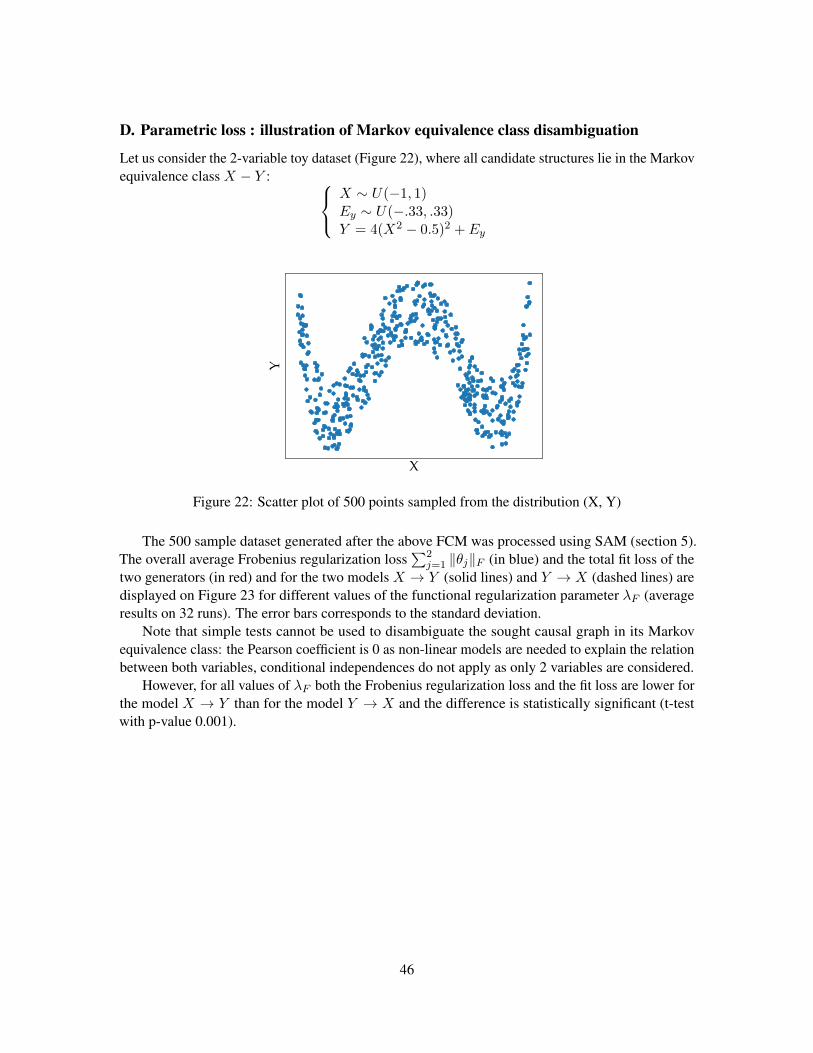
D. Parametric loss : illustration of Markov equivalence class disambiguation

Let us consider the 2-variable toy dataset (Figure 22), where all candidate structures lie in the Markovequivalence class X − Y :

X ∼ U(−1, 1)Ey ∼ U(−.33, .33)Y = 4(X2 − 0.5)2 + Ey

X

Y

Figure 22: Scatter plot of 500 points sampled from the distribution (X, Y)

The 500 sample dataset generated after the above FCM was processed using SAM (section 5).The overall average Frobenius regularization loss

∑2j=1 ‖θj‖F (in blue) and the total fit loss of the

two generators (in red) and for the two models X → Y (solid lines) and Y → X (dashed lines) aredisplayed on Figure 23 for different values of the functional regularization parameter λF (averageresults on 32 runs). The error bars corresponds to the standard deviation.

Note that simple tests cannot be used to disambiguate the sought causal graph in its Markovequivalence class: the Pearson coefficient is 0 as non-linear models are needed to explain the relationbetween both variables, conditional independences do not apply as only 2 variables are considered.

However, for all values of λF both the Frobenius regularization loss and the fit loss are lower forthe model X → Y than for the model Y → X and the difference is statistically significant (t-testwith p-value 0.001).

46

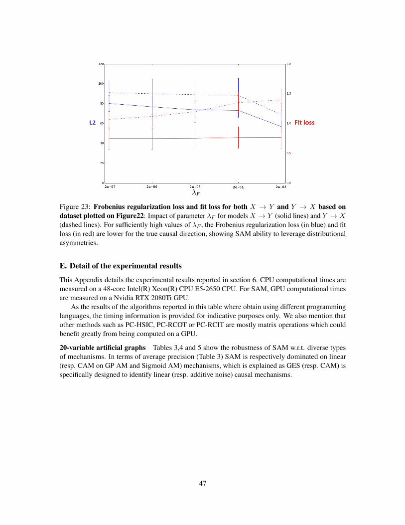
Figure 23: Frobenius regularization loss and fit loss for both X → Y and Y → X based ondataset plotted on Figure22: Impact of parameter λF for models X → Y (solid lines) and Y → X(dashed lines). For sufficiently high values of λF , the Frobenius regularization loss (in blue) and fitloss (in red) are lower for the true causal direction, showing SAM ability to leverage distributionalasymmetries.

E. Detail of the experimental results

This Appendix details the experimental results reported in section 6. CPU computational times aremeasured on a 48-core Intel(R) Xeon(R) CPU E5-2650 CPU. For SAM, GPU computational timesare measured on a Nvidia RTX 2080Ti GPU.

As the results of the algorithms reported in this table where obtain using different programminglanguages, the timing information is provided for indicative purposes only. We also mention thatother methods such as PC-HSIC, PC-RCOT or PC-RCIT are mostly matrix operations which couldbenefit greatly from being computed on a GPU.

20-variable artificial graphs Tables 3,4 and 5 show the robustness of SAM w.r.t. diverse typesof mechanisms. In terms of average precision (Table 3) SAM is respectively dominated on linear(resp. CAM on GP AM and Sigmoid AM) mechanisms, which is explained as GES (resp. CAM) isspecifically designed to identify linear (resp. additive noise) causal mechanisms.

47

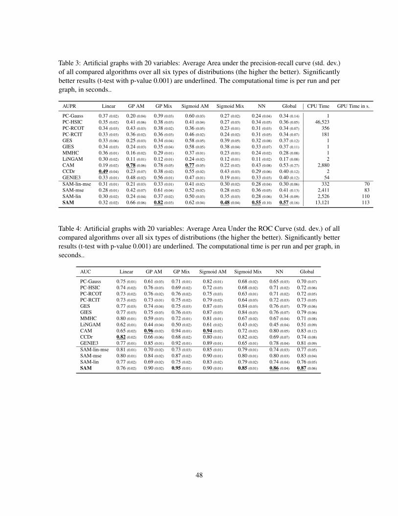
Table 3: Artificial graphs with 20 variables: Average Area under the precision-recall curve (std. dev.)of all compared algorithms over all six types of distributions (the higher the better). Significantlybetter results (t-test with p-value 0.001) are underlined. The computational time is per run and pergraph, in seconds..

AUPR Linear GP AM GP Mix Sigmoid AM Sigmoid Mix NN Global CPU Time GPU Time in s.

PC-Gauss 0.37 (0.02) 0.20 (0.04) 0.39 (0.03) 0.60 (0.03) 0.27 (0.02) 0.24 (0.04) 0.34 (0.14) 1PC-HSIC 0.35 (0.02) 0.41 (0.06) 0.38 (0.03) 0.41 (0.04) 0.27 (0.03) 0.34 (0.05) 0.36 (0.05) 46,523PC-RCOT 0.34 (0.03) 0.43 (0.03) 0.38 (0.02) 0.36 (0.05) 0.23 (0.01) 0.31 (0.03) 0.34 (0.07) 356PC-RCIT 0.33 (0.03) 0.36 (0.02) 0.36 (0.03) 0.46 (0.02) 0.24 (0.02) 0.31 (0.05) 0.34 (0.07) 181GES 0.33 (0.06) 0.25 (0.03) 0.34 (0.04) 0.58 (0.05) 0.39 (0.05) 0.32 (0.08) 0.37 (0.12) 1GIES 0.34 (0.03) 0.24 (0.03) 0.35 (0.04) 0.58 (0.05) 0.38 (0.04) 0.33 (0.07) 0.37 (0.11) 1MMHC 0.36 (0.01) 0.16 (0.02) 0.29 (0.01) 0.37 (0.01) 0.23 (0.01) 0.24 (0.02) 0.28 (0.08) 1LiNGAM 0.30 (0.02) 0.11 (0.01) 0.12 (0.01) 0.24 (0.02) 0.12 (0.01) 0.11 (0.02) 0.17 (0.08) 2CAM 0.19 (0.02) 0.78 (0.06) 0.78 (0.05) 0.77 (0.05) 0.22 (0.02) 0.43 (0.08) 0.53 (0.27) 2,880CCDr 0.49 (0.04) 0.23 (0.07) 0.38 (0.02) 0.55 (0.02) 0.43 (0.03) 0.29 (0.06) 0.40 (0.12) 2GENIE3 0.33 (0.01) 0.48 (0.02) 0.56 (0.01) 0.47 (0.01) 0.19 (0.01) 0.33 (0.03) 0.40 (0.12) 54SAM-lin-mse 0.31 (0.01) 0.21 (0.03) 0.33 (0.01) 0.41 (0.02) 0.30 (0.02) 0.28 (0.04) 0.30 (0.06) 332 70SAM-mse 0.28 (0.01) 0.42 (0.07) 0.61 (0.04) 0.52 (0.02) 0.28 (0.02) 0.36 (0.05) 0.41 (0.13) 2,411 83SAM-lin 0.30 (0.02) 0.24 (0.04) 0.37 (0.02) 0.50 (0.03) 0.35 (0.03) 0.28 (0.06) 0.34 (0.09) 2,526 110SAM 0.32 (0.02) 0.66 (0.06) 0.82 (0.03) 0.62 (0.04) 0.48 (0.04) 0.55 (0.10) 0.57 (0.16) 13,121 113

Table 4: Artificial graphs with 20 variables: Average Area Under the ROC Curve (std. dev.) of allcompared algorithms over all six types of distributions (the higher the better). Significantly betterresults (t-test with p-value 0.001) are underlined. The computational time is per run and per graph, inseconds..

AUC Linear GP AM GP Mix Sigmoid AM Sigmoid Mix NN Global

PC-Gauss 0.75 (0.01) 0.61 (0.03) 0.71 (0.01) 0.82 (0.01) 0.68 (0.02) 0.65 (0.03) 0.70 (0.07)

PC-HSIC 0.74 (0.02) 0.76 (0.03) 0.69 (0.02) 0.72 (0.03) 0.68 (0.02) 0.71 (0.02) 0.72 (0.06)

PC-RCOT 0.73 (0.02) 0.76 (0.02) 0.76 (0.02) 0.75 (0.03) 0.63 (0.01) 0.71 (0.02) 0.72 (0.05)

PC-RCIT 0.73 (0.02) 0.73 (0.01) 0.75 (0.02) 0.79 (0.02) 0.64 (0.03) 0.72 (0.03) 0.73 (0.05)

GES 0.77 (0.03) 0.74 (0.04) 0.75 (0.03) 0.87 (0.03) 0.84 (0.03) 0.76 (0.07) 0.79 (0.06)

GIES 0.77 (0.03) 0.75 (0.03) 0.76 (0.03) 0.87 (0.03) 0.84 (0.03) 0.76 (0.07) 0.79 (0.06)

MMHC 0.80 (0.01) 0.59 (0.03) 0.72 (0.01) 0.81 (0.01) 0.67 (0.02) 0.67 (0.04) 0.71 (0.08)

LiNGAM 0.62 (0.01) 0.44 (0.04) 0.50 (0.02) 0.61 (0.02) 0.43 (0.02) 0.45 (0.04) 0.51 (0.09)

CAM 0.65 (0.02) 0.96 (0.02) 0.94 (0.01) 0.94 (0.02) 0.72 (0.02) 0.80 (0.05) 0.83 (0.12)

CCDr 0.82 (0.02) 0.66 (0.06) 0.68 (0.02) 0.80 (0.01) 0.82 (0.02) 0.69 (0.07) 0.74 (0.08)

GENIE3 0.77 (0.01) 0.85 (0.01) 0.92 (0.01) 0.89 (0.01) 0.65 (0.01) 0.78 (0.04) 0.81 (0.09)

SAM-lin-mse 0.81 (0.01) 0.70 (0.02) 0.73 (0.03) 0.85 (0.01) 0.79 (0.01) 0.74 (0.03) 0.77 (0.05)

SAM-mse 0.80 (0.01) 0.84 (0.02) 0.87 (0.02) 0.90 (0.01) 0.80 (0.01) 0.80 (0.03) 0.83 (0.04)

SAM-lin 0.77 (0.02) 0.69 (0.02) 0.75 (0.02) 0.83 (0.02) 0.79 (0.02) 0.74 (0.04) 0.76 (0.05)

SAM 0.76 (0.02) 0.90 (0.02) 0.95 (0.01) 0.90 (0.01) 0.85 (0.01) 0.86 (0.04) 0.87 (0.06)

48

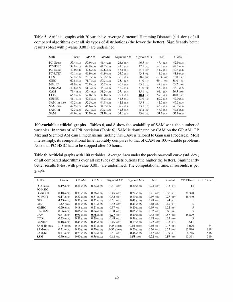
Table 5: Artificial graphs with 20 variables: Average Structural Hamming Distance (std. dev.) of allcompared algorithms over all six types of distributions (the lower the better). Significantly betterresults (t-test with p-value 0.001) are underlined.

SHD Linear GP AM GP Mix Sigmoid AM Sigmoid Mix NN Global

PC-Gauss 37.4 (1.0) 57.9 (4.0) 41.4 (2.2) 26.6 (1.7) 46.5 (2.1) 47.4 (2.0) 42.9 (9.9)

PC-HSIC 38.8 (2.0) 42.9 (3.1) 41.7 (5.2) 41.3 (2.2) 47.5 (3.3) 40.7 (2.0) 42.1 (6.1)

PC-RCOT 40.0 (1.4) 42.8 (3.2) 42.6 (1.8) 43.1 (2.1) 44.1 (0.5) 41.7 (2.1) 42.4 (2.4)

PC-RCIT 40.1 (1.2) 46.9 (1.8) 44.9 (1.7) 34.7 (1.1) 43.8 (0.5) 41.6 (1.8) 41.9 (4.2)

GES 59.2 (5.3) 70.7 (5.4) 50.2 (3.5) 36.0 (3.8) 58.6 (6.8) 67.3 (10.8) 57.0 (13.1)

GIES 60.8 (4.7) 71.7 (4.9) 50.3 (3.9) 35.4 (2.9) 61.0 (5.1) 69.1 (10.1) 58.0 (13.5)

MMHC 41.9 (1.4) 73.8 (5.0) 56.2 (1.9) 46.4 (1.2) 53.1 (1.3) 47.8 (2.7) 53.2 (10.6)

LiNGAM 40.8 (2.2) 51.3 (1.6) 48.3 (0.5) 42.2 (0.9) 51.0 (2.0) 55.9 (7.3) 48.3 (6.2)

CAM 79.4 (6.7) 37.4 (6.0) 38.3 (4.3) 37.4 (4.5) 85.1 (4.3) 61.4 (6.9) 56.5 (20.9)

CCDr 66.2 (6.2) 57.0 (5.6) 39.0 (1.6) 28.4 (2.7) 40.4 (1.9) 57.3 (9.8) 48.0 (14.2)

GENIE3 41.1 (3.6) 42.5 (2.9) 43.2 (4.1) 41.8 (3.5) 43.9 (5.2) 69.2 (9.2) 47.0 (6.9)

SAM-lin-mse 45.2 (1.1) 52.5 (2.3) 44.8 (1.1) 42.1 (1.4) 45.8 (1.7) 42.7 (1.5) 45.5 (3.7)

SAM-mse 47.9 (1.6) 46.6 (4.5) 34.7 (2.5) 37.2 (2.9) 53.1 (1.7) 43.7 (3.0) 43.9 (6.9)

SAM-lin 42.3 (2.3) 57.1 (3.9) 50.3 (3.7) 42.8 (3.9) 45.2 (2.3) 47.3 (4.0) 47.5 (6.1)

SAM 44.0 (2.1) 33.9 (4.8) 21.8 (2.9) 34.3 (2.8) 43.6 (2.5) 37.6 (4.6) 35.9 (8.2)

100-variable artificial graphs Tables 6, and 8 show the scalability of SAM w.r.t. the number ofvariables. In terms of AUPR precision (Table 6), SAM is dominated by CAM on the GP AM, GPMix and Sigmoid AM causal mechanisms (noting that CAM is tailored to Gaussian Processes). Mostinterestingly, its computational time favorably compares to that of CAM on 100-variable problems.Note that PC-HSIC had to be stopped after 50 hours.

Table 6: Artificial graphs with 100 variables: Average Area under the precision-recall curve (std. dev.)of all compared algorithms over all six types of distributions (the higher the better). Significantlybetter results (t-test with p-value 0.001) are underlined. The computational time, in seconds, is pergraph.

AUPR Linear GP AM GP Mix Sigmoid AM Sigmoid Mix NN Global CPU Time GPU Time

PC-Gauss 0.19 (0.01) 0.31 (0.02) 0.32 (0.02) 0.61 (0.02) 0.30 (0.01) 0.23 (0.03) 0.33 (0.13) 13PC-HSIC - - - - - - - -PC-RCOT 0.18 (0.01) 0.39 (0.02) 0.36 (0.01) 0.45 (0.01) 0.22 (0.01) 0.21 (0.02) 0.30 (0.11) 31,320PC-RCIT 0.17 (0.01) 0.32 (0.02) 0.31 (0.01) 0.52 (0.01) 0.19 (0.01) 0.19 (0.02) 0.27 (0.09) 46,440GES 0.53 (0.04) 0.32 (0.03) 0.32 (0.02) 0.61 (0.01) 0.41 (0.03) 0.48 (0.04) 0.44 (0.11) 1GIES 0.53 (0.03) 0.31 (0.03) 0.33 (0.02) 0.62 (0.02) 0.41 (0.02) 0.48 (0.04) 0.45 (0.11) 5MMHC 0.20 (0.01) 0.18 (0.01) 0.21 (0.01) 0.37 (0.01) 0.20 (0.01) 0.19 (0.01) 0.22 (0.07) 5LiNGAM 0.06 (0.01) 0.06 (0.01) 0.04 (0.01) 0.08 (0.01) 0.05 (0.01) 0.07 (0.01) 0.06 (0.01) 5CAM 0.31 (0.01) 0.93 (0.01) 0.78 (0.01) 0.77 (0.01) 0.20 (0.01) 0.43 (0.05) 0.57 (0.28) 45,899CCDr 0.23 (0.01) 0.31 (0.04) 0.26 (0.02) 0.49 (0.02) 0.39 (0.02) 0.38 (0.05) 0.35 (0.09) 3GENIE3 0.18 (0.01) 0.48 (0.02) 0.45 (0.01) 0.45 (0.01) 0.19 (0.01) 0.22 (0.02) 0.33 (0.13) 511SAM-lin-mse 0.15 (0.003) 0.16 (0.02) 0.13 (0.01) 0.25 (0.004) 0.16 (0.002) 0.16 (0.01) 0.17 (0.04) 3,076 74SAM-mse 0.21 (0.01) 0.30 (0.03) 0.20 (0.01) 0.33 (0.005) 0.20 (0.01) 0.26 (0.03) 0.25 (0.05) 12,896 118SAM-lin 0.41 (0.01) 0.29 (0.02) 0.22 (0.01) 0.51 (0.01) 0.46 (0.02) 0.47 (0.04) 0.39 (0.11) 8,746 516SAM 0.50 (0.02) 0.60 (0.04) 0.56 (0.02) 0.62 (0.02) 0.55 (0.02) 0.72 (0.03) 0.59 (0.08) 15,361 519

49

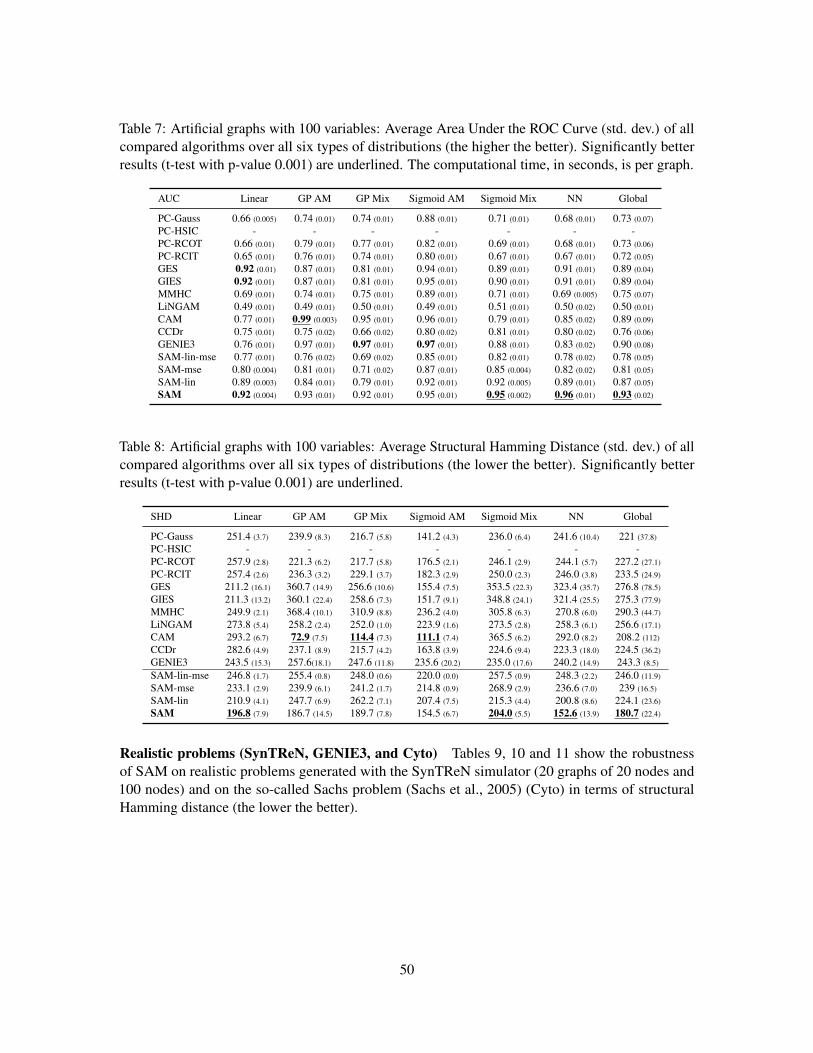
Table 7: Artificial graphs with 100 variables: Average Area Under the ROC Curve (std. dev.) of allcompared algorithms over all six types of distributions (the higher the better). Significantly betterresults (t-test with p-value 0.001) are underlined. The computational time, in seconds, is per graph.

AUC Linear GP AM GP Mix Sigmoid AM Sigmoid Mix NN Global

PC-Gauss 0.66 (0.005) 0.74 (0.01) 0.74 (0.01) 0.88 (0.01) 0.71 (0.01) 0.68 (0.01) 0.73 (0.07)

PC-HSIC - - - - - - -PC-RCOT 0.66 (0.01) 0.79 (0.01) 0.77 (0.01) 0.82 (0.01) 0.69 (0.01) 0.68 (0.01) 0.73 (0.06)

PC-RCIT 0.65 (0.01) 0.76 (0.01) 0.74 (0.01) 0.80 (0.01) 0.67 (0.01) 0.67 (0.01) 0.72 (0.05)

GES 0.92 (0.01) 0.87 (0.01) 0.81 (0.01) 0.94 (0.01) 0.89 (0.01) 0.91 (0.01) 0.89 (0.04)

GIES 0.92 (0.01) 0.87 (0.01) 0.81 (0.01) 0.95 (0.01) 0.90 (0.01) 0.91 (0.01) 0.89 (0.04)

MMHC 0.69 (0.01) 0.74 (0.01) 0.75 (0.01) 0.89 (0.01) 0.71 (0.01) 0.69 (0.005) 0.75 (0.07)

LiNGAM 0.49 (0.01) 0.49 (0.01) 0.50 (0.01) 0.49 (0.01) 0.51 (0.01) 0.50 (0.02) 0.50 (0.01)

CAM 0.77 (0.01) 0.99 (0.003) 0.95 (0.01) 0.96 (0.01) 0.79 (0.01) 0.85 (0.02) 0.89 (0.09)

CCDr 0.75 (0.01) 0.75 (0.02) 0.66 (0.02) 0.80 (0.02) 0.81 (0.01) 0.80 (0.02) 0.76 (0.06)

GENIE3 0.76 (0.01) 0.97 (0.01) 0.97 (0.01) 0.97 (0.01) 0.88 (0.01) 0.83 (0.02) 0.90 (0.08)

SAM-lin-mse 0.77 (0.01) 0.76 (0.02) 0.69 (0.02) 0.85 (0.01) 0.82 (0.01) 0.78 (0.02) 0.78 (0.05)

SAM-mse 0.80 (0.004) 0.81 (0.01) 0.71 (0.02) 0.87 (0.01) 0.85 (0.004) 0.82 (0.02) 0.81 (0.05)

SAM-lin 0.89 (0.003) 0.84 (0.01) 0.79 (0.01) 0.92 (0.01) 0.92 (0.005) 0.89 (0.01) 0.87 (0.05)

SAM 0.92 (0.004) 0.93 (0.01) 0.92 (0.01) 0.95 (0.01) 0.95 (0.002) 0.96 (0.01) 0.93 (0.02)

Table 8: Artificial graphs with 100 variables: Average Structural Hamming Distance (std. dev.) of allcompared algorithms over all six types of distributions (the lower the better). Significantly betterresults (t-test with p-value 0.001) are underlined.

SHD Linear GP AM GP Mix Sigmoid AM Sigmoid Mix NN Global

PC-Gauss 251.4 (3.7) 239.9 (8.3) 216.7 (5.8) 141.2 (4.3) 236.0 (6.4) 241.6 (10.4) 221 (37.8)

PC-HSIC - - - - - - -PC-RCOT 257.9 (2.8) 221.3 (6.2) 217.7 (5.8) 176.5 (2.1) 246.1 (2.9) 244.1 (5.7) 227.2 (27.1)

PC-RCIT 257.4 (2.6) 236.3 (3.2) 229.1 (3.7) 182.3 (2.9) 250.0 (2.3) 246.0 (3.8) 233.5 (24.9)

GES 211.2 (16.1) 360.7 (14.9) 256.6 (10.6) 155.4 (7.5) 353.5 (22.3) 323.4 (35.7) 276.8 (78.5)

GIES 211.3 (13.2) 360.1 (22.4) 258.6 (7.3) 151.7 (9.1) 348.8 (24.1) 321.4 (25.5) 275.3 (77.9)

MMHC 249.9 (2.1) 368.4 (10.1) 310.9 (8.8) 236.2 (4.0) 305.8 (6.3) 270.8 (6.0) 290.3 (44.7)

LiNGAM 273.8 (5.4) 258.2 (2.4) 252.0 (1.0) 223.9 (1.6) 273.5 (2.8) 258.3 (6.1) 256.6 (17.1)

CAM 293.2 (6.7) 72.9 (7.5) 114.4 (7.3) 111.1 (7.4) 365.5 (6.2) 292.0 (8.2) 208.2 (112)

CCDr 282.6 (4.9) 237.1 (8.9) 215.7 (4.2) 163.8 (3.9) 224.6 (9.4) 223.3 (18.0) 224.5 (36.2)

GENIE3 243.5 (15.3) 257.6(18.1) 247.6 (11.8) 235.6 (20.2) 235.0 (17.6) 240.2 (14.9) 243.3 (8.5)

SAM-lin-mse 246.8 (1.7) 255.4 (0.8) 248.0 (0.6) 220.0 (0.0) 257.5 (0.9) 248.3 (2.2) 246.0 (11.9)

SAM-mse 233.1 (2.9) 239.9 (6.1) 241.2 (1.7) 214.8 (0.9) 268.9 (2.9) 236.6 (7.0) 239 (16.5)

SAM-lin 210.9 (4.1) 247.7 (6.9) 262.2 (7.1) 207.4 (7.5) 215.3 (4.4) 200.8 (8.6) 224.1 (23.6)

SAM 196.8 (7.9) 186.7 (14.5) 189.7 (7.8) 154.5 (6.7) 204.0 (5.5) 152.6 (13.9) 180.7 (22.4)

Realistic problems (SynTReN, GENIE3, and Cyto) Tables 9, 10 and 11 show the robustnessof SAM on realistic problems generated with the SynTReN simulator (20 graphs of 20 nodes and100 nodes) and on the so-called Sachs problem (Sachs et al., 2005) (Cyto) in terms of structuralHamming distance (the lower the better).

50

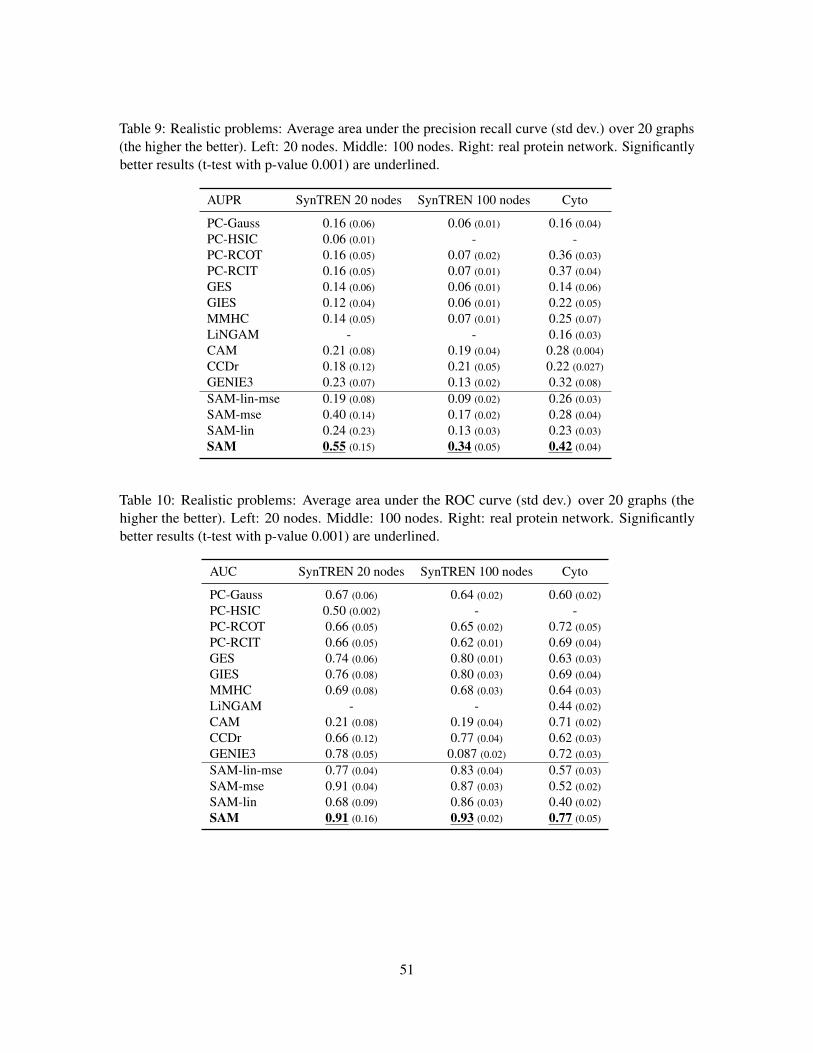
Table 9: Realistic problems: Average area under the precision recall curve (std dev.) over 20 graphs(the higher the better). Left: 20 nodes. Middle: 100 nodes. Right: real protein network. Significantlybetter results (t-test with p-value 0.001) are underlined.

AUPR SynTREN 20 nodes SynTREN 100 nodes Cyto

PC-Gauss 0.16 (0.06) 0.06 (0.01) 0.16 (0.04)PC-HSIC 0.06 (0.01) - -PC-RCOT 0.16 (0.05) 0.07 (0.02) 0.36 (0.03)PC-RCIT 0.16 (0.05) 0.07 (0.01) 0.37 (0.04)GES 0.14 (0.06) 0.06 (0.01) 0.14 (0.06)GIES 0.12 (0.04) 0.06 (0.01) 0.22 (0.05)MMHC 0.14 (0.05) 0.07 (0.01) 0.25 (0.07)LiNGAM - - 0.16 (0.03)CAM 0.21 (0.08) 0.19 (0.04) 0.28 (0.004)CCDr 0.18 (0.12) 0.21 (0.05) 0.22 (0.027)GENIE3 0.23 (0.07) 0.13 (0.02) 0.32 (0.08)

SAM-lin-mse 0.19 (0.08) 0.09 (0.02) 0.26 (0.03)SAM-mse 0.40 (0.14) 0.17 (0.02) 0.28 (0.04)SAM-lin 0.24 (0.23) 0.13 (0.03) 0.23 (0.03)SAM 0.55 (0.15) 0.34 (0.05) 0.42 (0.04)

Table 10: Realistic problems: Average area under the ROC curve (std dev.) over 20 graphs (thehigher the better). Left: 20 nodes. Middle: 100 nodes. Right: real protein network. Significantlybetter results (t-test with p-value 0.001) are underlined.

AUC SynTREN 20 nodes SynTREN 100 nodes Cyto

PC-Gauss 0.67 (0.06) 0.64 (0.02) 0.60 (0.02)PC-HSIC 0.50 (0.002) - -PC-RCOT 0.66 (0.05) 0.65 (0.02) 0.72 (0.05)PC-RCIT 0.66 (0.05) 0.62 (0.01) 0.69 (0.04)GES 0.74 (0.06) 0.80 (0.01) 0.63 (0.03)GIES 0.76 (0.08) 0.80 (0.03) 0.69 (0.04)MMHC 0.69 (0.08) 0.68 (0.03) 0.64 (0.03)LiNGAM - - 0.44 (0.02)CAM 0.21 (0.08) 0.19 (0.04) 0.71 (0.02)CCDr 0.66 (0.12) 0.77 (0.04) 0.62 (0.03)GENIE3 0.78 (0.05) 0.087 (0.02) 0.72 (0.03)

SAM-lin-mse 0.77 (0.04) 0.83 (0.04) 0.57 (0.03)SAM-mse 0.91 (0.04) 0.87 (0.03) 0.52 (0.02)SAM-lin 0.68 (0.09) 0.86 (0.03) 0.40 (0.02)SAM 0.91 (0.16) 0.93 (0.02) 0.77 (0.05)

51

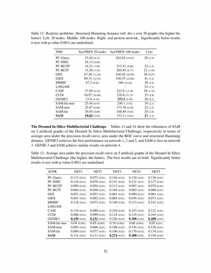
Table 11: Realistic problems: Structural Hamming distance (std. dev.) over 20 graphs (the higher thebetter). Left: 20 nodes. Middle: 100 nodes. Right: real protein network.. Significantly better results(t-test with p-value 0.001) are underlined.

SHD SynTREN 20 nodes SynTREN 100 nodes Cyto

PC-Gauss 53.42 (6.13) 262.65 (19.87) 28 (2.9)PC-HSIC 24.13 (4.08) - -PC-RCOT 34.21 (7.99) 213.51 (8.60) 22 (1.9)PC-RCIT 33.20 (7.54) 204.95 (8.77) 23 (1.49)GES 67.26 (12.26) 436.02 (18.99) 38 (0.47)GIES 69.31 (12.55) 430.55 (22.80) 41 (3.2)MMHC 67.2 (8.42) 346 (14.44) 38 (3.4)LiNGAM - - 23 (3.2)CAM 57.85 (9.10) 222.9 (12.38) 28 (1.32)CCDr 54.97 (16.68) 228.8 (21.15) 35 (4.8)GENIE3 23.6 (4.14) 153.2 (4.59) 20 (4.1)

SAM-lin-mse 25.44 (4.97) 240.1 (3.92) 19 (2.1)SAM-mse 25.67 (6.96) 173.78 (6.36) 22 (3.2)SAM-lin 30.45 (8.09) 168.89 (5.63) 20 (2.8)SAM 19.02 (5.83) 153.5 (13.03) 17 (3.2)

The Dream4 In Silico Multifactorial Challenge. Tables 13 and 14 show the robustness of SAMon 5 artificial graphs of the Dream4 In Silico Multifactorial Challenge, respectively in terms ofaverage area under the precision recall curve, area under the ROC curve and structural Hammingdistance. GENIE3 achieves the best performance on network 1, 2 and 5, and SAM is first on network3. GENIE 3 and SAM achieve similar results on network 4.

Table 12: Average area under the precision recall curve on 5 artificial graphs of the Dream4 In SilicoMultifactorial Challenge (the higher, the better). The best results are in bold. Significantly betterresults (t-test with p-value 0.001) are underlined.

AUPR NET1 NET2 NET3 NET4 NET5

PC-Gauss 0.113 (0.01) 0.072 (0.01) 0.144 (0.02) 0.130 (0.01) 0.136 (0.01)PC-HSIC 0.116 (0.01) 0.070 (0.01) 0.151 (0.02) 0.121 (0.01) 0.127 (0.02)PC-RCOT 0.094 (0.02) 0.054 (0.01) 0.113 (0.01) 0.097 (0.01) 0.079 (0.01)PC-RCIT 0.084 (0.01) 0.046 (0.01) 0.104 (0.01) 0.083 (0.01) 0.086 (0.01)GES 0.051 (0.01) 0.053 (0.01) 0.061 (0.01) 0.080 (0.01) 0.081 (0.01)GIES 0.047 (0.01) 0.062 (0.01) 0.065 (0.01) 0.076 (0.01) 0.073 (0.01)MMHC 0.116 (0.01) 0.073 (0.01) 0.148 (0.02) 0.133 (0.01) 0.141 (0.02)LiNGAM - - - - -CAM 0.116 (0.01) 0.080 (0.01) 0.210 (0.02) 0.147 (0.02) 0.121 (0.01)CCDr 0.088 (0.01) 0.099 (0.01) 0.114 (0.01) 0.119 (0.01) 0.165 (0.02)GENIE3 0.159 (0.01) 0.151 (0.02) 0.226 (0.02) 0.208 (0.02) 0.209 (0.02)

SAM-lin-mse 0.04 (0.001) 0.05 (0.001) 0.10 (0.002) 0.08 (0.001) 0.05 (0.01)SAM-mse 0.095 (0.01) 0.066 (0.01) 0.188 (0.02) 0.145 (0.01) 0.136 (0.01)SAM-lin 0.080 (0.01) 0.077 (0.01) 0.190 (0.02) 0.170 (0.02) 0.134 (0.01)SAM 0.131 (0.01) 0.111 (0.01) 0.274 (0.03) 0.208 (0.02) 0.194 (0.02)

52

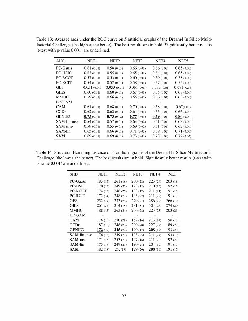
Table 13: Average area under the ROC curve on 5 artificial graphs of the Dream4 In Silico Multi-factorial Challenge (the higher, the better). The best results are in bold. Significantly better results(t-test with p-value 0.001) are underlined.

AUC NET1 NET2 NET3 NET4 NET5

PC-Gauss 0.61 (0.01) 0.58 (0.01) 0.66 (0.01) 0.66 (0.02) 0.65 (0.01)PC-HSIC 0.63 (0.01) 0.55 (0.01) 0.65 (0.01) 0.64 (0.01) 0.65 (0.01)PC-RCOT 0.57 (0.01) 0.53 (0.01) 0.60 (0.01) 0.59 (0.01) 0.58 (0.01)PC-RCIT 0.54 (0.01) 0.52 (0.01) 0.58 (0.01) 0.57 (0.01) 0.55 (0.01)GES 0.051 (0.01) 0.053 (0.01) 0.061 (0.01) 0.080 (0.01) 0.081 (0.01)GIES 0.60 (0.01) 0.60 (0.01) 0.67 (0.01) 0.65 (0.02) 0.68 (0.01)MMHC 0.59 (0.01) 0.66 (0.01) 0.65 (0.02) 0.66 (0.01) 0.63 (0.01)LiNGAM - - - - -CAM 0.61 (0.01) 0.68 (0.01) 0.70 (0.02) 0.68 (0.01) 0.67(0.01)CCDr 0.62 (0.01) 0.62 (0.01) 0.64 (0.01) 0.66 (0.01) 0.66 (0.01)GENIE3 0.75 (0.01) 0.73 (0.02) 0.77 (0.01) 0.79 (0.01) 0.80 (0.01)

SAM-lin-mse 0.54 (0.01) 0.57 (0.01) 0.63 (0.02) 0.61 (0.01) 0.63 (0.01)SAM-mse 0.59 (0.01) 0.55 (0.01) 0.69 (0.02) 0.61 (0.01) 0.62 (0.01)SAM-lin 0.65 (0.01) 0.66 (0.01) 0.71 (0.02) 0.69 (0.02) 0.71 (0.01)SAM 0.69 (0.01) 0.69 (0.01) 0.73 (0.02) 0.73 (0.02) 0.77 (0.02)

Table 14: Structural Hamming distance on 5 artificial graphs of the Dream4 In Silico MultifactorialChallenge (the lower, the better). The best results are in bold. Significantly better results (t-test withp-value 0.001) are underlined.

SHD NET1 NET2 NET3 NET4 NET

PC-Gauss 183 (15) 261 (18) 200 (22) 223 (24) 203 (18)PC-HSIC 170 (15) 249 (25) 193 (18) 210 (16) 192 (15)PC-RCOT 174 (15) 248 (26) 193 (17) 211 (21) 191 (17)PC-RCIT 172 (14) 248 (23) 193 (22) 211 (22) 191 (17)GES 252 (27) 333 (26) 279 (21) 286 (22) 266 (19)GIES 261 (27) 314 (18) 281 (31) 304 (26) 274 (20)MMHC 188 (15) 263 (24) 206 (22) 223 (23) 203 (21)LiNGAM - - - - -CAM 178 (15) 250 (21) 182 (16) 213 (14) 196 (15)CCDr 187 (15) 248 (20) 209 (20) 227 (22) 189 (22)GENIE3 172 (17) 245 (22) 190 (17) 208 (19) 193 (20)

SAM-lin-mse 176 (16) 249 (23) 195 (25) 211 (24) 193 (19)SAM-mse 171 (15) 253 (23) 197 (16) 211 (20) 192 (23)SAM-lin 175 (17) 249 (25) 190 (21) 204 (19) 191 (17)SAM 182 (18) 252(19) 179 (20) 208 (19) 191 (17)

53

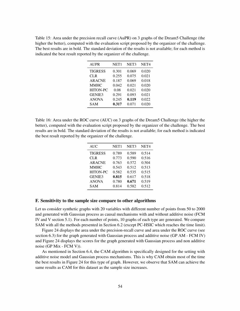
Table 15: Area under the precision recall curve (AuPR) on 3 graphs of the Dream5 Challenge (thehigher the better), computed with the evaluation script proposed by the organizer of the challenge.The best results are in bold. The standard deviation of the results is not available; for each method isindicated the best result reported by the organizer of the challenge.

AUPR NET1 NET3 NET4

TIGRESS 0.301 0.069 0.020CLR 0.255 0.075 0.021ARACNE 0.187 0.069 0.018MMHC 0.042 0.021 0.020HITON-PC 0.08 0.021 0.020GENIE3 0.291 0.093 0.021ANOVA 0.245 0.119 0.022SAM 0.317 0.071 0.020

Table 16: Area under the ROC curve (AUC) on 3 graphs of the Dream5 Challenge (the higher thebetter), computed with the evaluation script proposed by the organizer of the challenge. The bestresults are in bold. The standard deviation of the results is not available; for each method is indicatedthe best result reported by the organizer of the challenge.

AUC NET1 NET3 NET4

TIGRESS 0.789 0.589 0.514CLR 0.773 0.590 0.516ARACNE 0.763 0.572 0.504MMHC 0.543 0.512 0.513HITON-PC 0.582 0.535 0.515GENIE3 0.815 0.617 0.518ANOVA 0.780 0.671 0.519SAM 0.814 0.582 0.512

F. Sensitivity to the sample size compare to other algorithms

Let us consider synthetic graphs with 20 variables with different number of points from 50 to 2000and generated with Gaussian process as causal mechanisms with and without additive noise (FCMIV and V section 5.1). For each number of points, 10 graphs of each type are generated. We compareSAM with all the methods presented in Section 6.2 (except PC-HSIC which reaches the time limit).

Figure 24 displays the area under the precision-recall curve and area under the ROC curve (seesection 6.3) for the graph generated with Gaussian process and additive noise (GP AM - FCM IV)and Figure 24 displays the scores for the graph generated with Gaussian process and non additivenoise (GP Mix - FCM V)).

As mentioned in Section 6.4, the CAM algorithm is specifically designed for the setting withadditive noise model and Gaussian process mechanisms. This is why CAM obtain most of the timethe best results in Figure 24 for this type of graph. However, we observe that SAM can achieve thesame results as CAM for this dataset as the sample size increases.

54

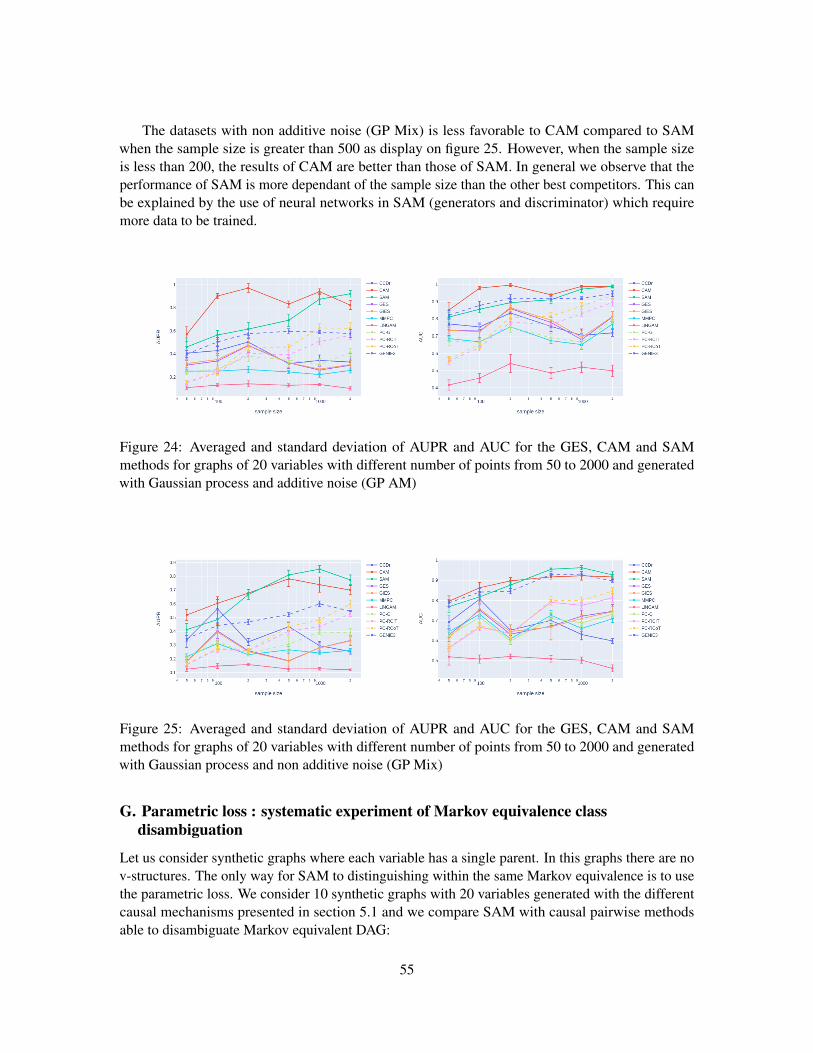
The datasets with non additive noise (GP Mix) is less favorable to CAM compared to SAMwhen the sample size is greater than 500 as display on figure 25. However, when the sample sizeis less than 200, the results of CAM are better than those of SAM. In general we observe that theperformance of SAM is more dependant of the sample size than the other best competitors. This canbe explained by the use of neural networks in SAM (generators and discriminator) which requiremore data to be trained.

Figure 24: Averaged and standard deviation of AUPR and AUC for the GES, CAM and SAMmethods for graphs of 20 variables with different number of points from 50 to 2000 and generatedwith Gaussian process and additive noise (GP AM)

Figure 25: Averaged and standard deviation of AUPR and AUC for the GES, CAM and SAMmethods for graphs of 20 variables with different number of points from 50 to 2000 and generatedwith Gaussian process and non additive noise (GP Mix)

G. Parametric loss : systematic experiment of Markov equivalence classdisambiguation

Let us consider synthetic graphs where each variable has a single parent. In this graphs there are nov-structures. The only way for SAM to distinguishing within the same Markov equivalence is to usethe parametric loss. We consider 10 synthetic graphs with 20 variables generated with the differentcausal mechanisms presented in section 5.1 and we compare SAM with causal pairwise methodsable to disambiguate Markov equivalent DAG:

55

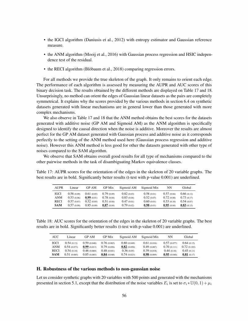
• the IGCI algorithm (Daniusis et al., 2012) with entropy estimator and Gaussian referencemeasure.

• the ANM algorithm (Mooij et al., 2016) with Gaussian process regression and HSIC indepen-dence test of the residual.

• the RECI algorithm (Blobaum et al., 2018) comparing regression errors.

For all methods we provide the true skeleton of the graph. It only remains to orient each edge.The performance of each algorithm is assessed by measuring the AUPR and AUC scores of thisbinary decision task. The results obtained by the different methods are displayed on Table 17 and 18.Unsurprisingly, no method can orient the edges of Gaussian linear datasets as the pairs are completelysymmetrical. It explains why the scores provided by the various methods in section 6.4 on syntheticdatasets generated with linear mechanisms are in general lower than those generated with morecomplex mechanisms.

We also observe in Table 17 and 18 that the ANM method obtains the best scores for the datasetsgenerated with additive noise (GP AM and Sigmoid AM) as the ANM algorithm is specificallydesigned to identify the causal direction when the noise is additive. Moreover the results are almostperfect for the GP AM dataset generated with Gaussian process and additive noise as it correspondsperfectly to the setting of the ANM method used here (Gaussian process regression and additivenoise). However this ANM method is less good for other the datasets generated with other type ofnoises compared to the SAM algorithm.

We observe that SAM obtains overall good results for all type of mechanisms compared to theother pairwise methods in the task of disambiguating Markov equivalence classes.

Table 17: AUPR scores for the orientation of the edges in the skeleton of 20 variable graphs. Thebest results are in bold. Significantly better results (t-test with p-value 0.001) are underlined.

AUPR Linear GP AM GP Mix Sigmoid AM Sigmoid Mix NN Global

IGCI 0.58 (0.09) 0.61 (0.05) 0.79 (0.09) 0.82 (0.03) 0.58 (0.01) 0.57 (0.04) 0.66 (0.12)

ANM 0.53 (0.06) 0.99 (0.01) 0.78 (0.04) 0.83 (0.04) 0.52 (0.07) 0.72 (0.08) 0.73 (0.17)

RECI 0.57 (0.07) 0.52 (0.05) 0.51 (0.04) 0.47 (0.01) 0.60 (0.01) 0.53 (0.10) 0.54 (0.07)

SAM 0.57 (0.09) 0.85 (0.09) 0.87 (0.04) 0.79 (0.02) 0.98 (0.01) 0.95 (0.04) 0.83 (0.15)

Table 18: AUC scores for the orientation of the edges in the skeleton of 20 variable graphs. The bestresults are in bold. Significantly better results (t-test with p-value 0.001) are underlined.

AUC Linear GP AM GP Mix Sigmoid AM Sigmoid Mix NN Global

IGCI 0.54 (0.13) 0.59 (0.048) 0.76 (0.083) 0.80 (0.049) 0.61 (0.016) 0.57 (0.077) 0.64 (0.13)

ANM 0.54 (0.073) 0.99 (0.013) 0.79 (0.056) 0.82 (0.050) 0.49 (0.087) 0.70 (0.111) 0.72 (0.185)

RECI 0.54 (0.10) 0.46 (0.069) 0.48 (0.041) 0.36 (0.05) 0.39 (0.018) 0.44 (0.18) 0.45 (0.11)

SAM 0.51 (0.085) 0.85 (0.085) 0.84 (0.048) 0.74 (0.023) 0.98 (0.009) 0.95 (0.040) 0.81 (0.17)

H. Robustness of the various methods to non-gaussian noise

Let us consider synthetic graphs with 20 variables with 500 points and generated with the mechanismspresented in section 5.1, except that the distribution of the noise variablesEi is set to σi ∗U(0, 1)+µi

56

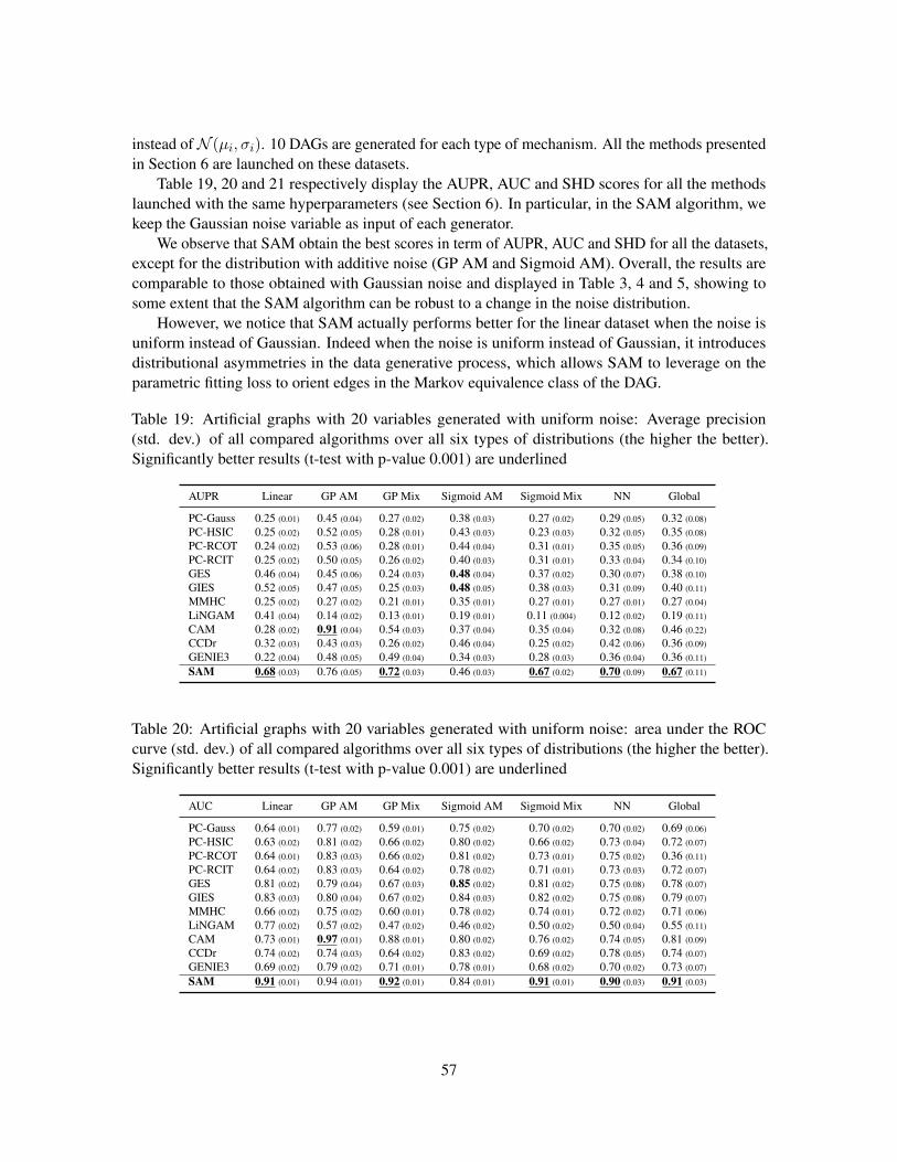
instead ofN (µi, σi). 10 DAGs are generated for each type of mechanism. All the methods presentedin Section 6 are launched on these datasets.

Table 19, 20 and 21 respectively display the AUPR, AUC and SHD scores for all the methodslaunched with the same hyperparameters (see Section 6). In particular, in the SAM algorithm, wekeep the Gaussian noise variable as input of each generator.

We observe that SAM obtain the best scores in term of AUPR, AUC and SHD for all the datasets,except for the distribution with additive noise (GP AM and Sigmoid AM). Overall, the results arecomparable to those obtained with Gaussian noise and displayed in Table 3, 4 and 5, showing tosome extent that the SAM algorithm can be robust to a change in the noise distribution.

However, we notice that SAM actually performs better for the linear dataset when the noise isuniform instead of Gaussian. Indeed when the noise is uniform instead of Gaussian, it introducesdistributional asymmetries in the data generative process, which allows SAM to leverage on theparametric fitting loss to orient edges in the Markov equivalence class of the DAG.

Table 19: Artificial graphs with 20 variables generated with uniform noise: Average precision(std. dev.) of all compared algorithms over all six types of distributions (the higher the better).Significantly better results (t-test with p-value 0.001) are underlined

AUPR Linear GP AM GP Mix Sigmoid AM Sigmoid Mix NN Global

PC-Gauss 0.25 (0.01) 0.45 (0.04) 0.27 (0.02) 0.38 (0.03) 0.27 (0.02) 0.29 (0.05) 0.32 (0.08)

PC-HSIC 0.25 (0.02) 0.52 (0.05) 0.28 (0.01) 0.43 (0.03) 0.23 (0.03) 0.32 (0.05) 0.35 (0.08)

PC-RCOT 0.24 (0.02) 0.53 (0.06) 0.28 (0.01) 0.44 (0.04) 0.31 (0.01) 0.35 (0.05) 0.36 (0.09)

PC-RCIT 0.25 (0.02) 0.50 (0.05) 0.26 (0.02) 0.40 (0.03) 0.31 (0.01) 0.33 (0.04) 0.34 (0.10)

GES 0.46 (0.04) 0.45 (0.06) 0.24 (0.03) 0.48 (0.04) 0.37 (0.02) 0.30 (0.07) 0.38 (0.10)

GIES 0.52 (0.05) 0.47 (0.05) 0.25 (0.03) 0.48 (0.05) 0.38 (0.03) 0.31 (0.09) 0.40 (0.11)

MMHC 0.25 (0.02) 0.27 (0.02) 0.21 (0.01) 0.35 (0.01) 0.27 (0.01) 0.27 (0.01) 0.27 (0.04)

LiNGAM 0.41 (0.04) 0.14 (0.02) 0.13 (0.01) 0.19 (0.01) 0.11 (0.004) 0.12 (0.02) 0.19 (0.11)

CAM 0.28 (0.02) 0.91 (0.04) 0.54 (0.03) 0.37 (0.04) 0.35 (0.04) 0.32 (0.08) 0.46 (0.22)

CCDr 0.32 (0.03) 0.43 (0.03) 0.26 (0.02) 0.46 (0.04) 0.25 (0.02) 0.42 (0.06) 0.36 (0.09)

GENIE3 0.22 (0.04) 0.48 (0.05) 0.49 (0.04) 0.34 (0.03) 0.28 (0.03) 0.36 (0.04) 0.36 (0.11)

SAM 0.68 (0.03) 0.76 (0.05) 0.72 (0.03) 0.46 (0.03) 0.67 (0.02) 0.70 (0.09) 0.67 (0.11)

Table 20: Artificial graphs with 20 variables generated with uniform noise: area under the ROCcurve (std. dev.) of all compared algorithms over all six types of distributions (the higher the better).Significantly better results (t-test with p-value 0.001) are underlined

AUC Linear GP AM GP Mix Sigmoid AM Sigmoid Mix NN Global

PC-Gauss 0.64 (0.01) 0.77 (0.02) 0.59 (0.01) 0.75 (0.02) 0.70 (0.02) 0.70 (0.02) 0.69 (0.06)

PC-HSIC 0.63 (0.02) 0.81 (0.02) 0.66 (0.02) 0.80 (0.02) 0.66 (0.02) 0.73 (0.04) 0.72 (0.07)

PC-RCOT 0.64 (0.01) 0.83 (0.03) 0.66 (0.02) 0.81 (0.02) 0.73 (0.01) 0.75 (0.02) 0.36 (0.11)

PC-RCIT 0.64 (0.02) 0.83 (0.03) 0.64 (0.02) 0.78 (0.02) 0.71 (0.01) 0.73 (0.03) 0.72 (0.07)

GES 0.81 (0.02) 0.79 (0.04) 0.67 (0.03) 0.85 (0.02) 0.81 (0.02) 0.75 (0.08) 0.78 (0.07)

GIES 0.83 (0.03) 0.80 (0.04) 0.67 (0.02) 0.84 (0.03) 0.82 (0.02) 0.75 (0.08) 0.79 (0.07)

MMHC 0.66 (0.02) 0.75 (0.02) 0.60 (0.01) 0.78 (0.02) 0.74 (0.01) 0.72 (0.02) 0.71 (0.06)

LiNGAM 0.77 (0.02) 0.57 (0.02) 0.47 (0.02) 0.46 (0.02) 0.50 (0.02) 0.50 (0.04) 0.55 (0.11)

CAM 0.73 (0.01) 0.97 (0.01) 0.88 (0.01) 0.80 (0.02) 0.76 (0.02) 0.74 (0.05) 0.81 (0.09)

CCDr 0.74 (0.02) 0.74 (0.03) 0.64 (0.02) 0.83 (0.02) 0.69 (0.02) 0.78 (0.05) 0.74 (0.07)

GENIE3 0.69 (0.02) 0.79 (0.02) 0.71 (0.01) 0.78 (0.01) 0.68 (0.02) 0.70 (0.02) 0.73 (0.07)

SAM 0.91 (0.01) 0.94 (0.01) 0.92 (0.01) 0.84 (0.01) 0.91 (0.01) 0.90 (0.03) 0.91 (0.03)

57

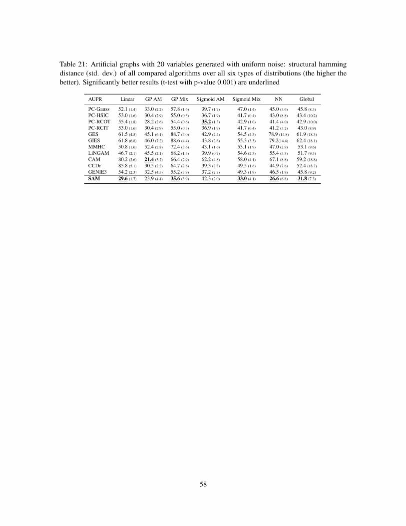
Table 21: Artificial graphs with 20 variables generated with uniform noise: structural hammingdistance (std. dev.) of all compared algorithms over all six types of distributions (the higher thebetter). Significantly better results (t-test with p-value 0.001) are underlined

AUPR Linear GP AM GP Mix Sigmoid AM Sigmoid Mix NN Global

PC-Gauss 52.1 (1.4) 33.0 (2.2) 57.8 (1.6) 39.7 (1.7) 47.0 (1.4) 45.0 (3.6) 45.8 (8.3)

PC-HSIC 53.0 (1.6) 30.4 (2.9) 55.0 (0.3) 36.7 (1.9) 41.7 (0.4) 43.0 (8.8) 43.4 (10.2)

PC-RCOT 55.4 (1.8) 28.2 (2.6) 54.4 (0.6) 35.2 (1.3) 42.9 (1.0) 41.4 (4.0) 42.9 (10.0)

PC-RCIT 53.0 (1.6) 30.4 (2.9) 55.0 (0.3) 36.9 (1.9) 41.7 (0.4) 41.2 (3.2) 43.0 (8.9)

GES 61.5 (4.5) 45.1 (6.1) 88.7 (4.0) 42.9 (2.4) 54.5 (4.5) 78.9 (14.8) 61.9 (18.3)

GIES 61.8 (6.8) 46.0 (7.2) 88.6 (4.4) 43.8 (2.6) 55.3 (3.3) 79.2(14.4) 62.4 (18.1)

MMHC 50.8 (1.6) 52.4 (2.8) 72.4 (3.6) 43.1 (1.6) 53.1 (1.9) 47.0 (2.9) 53.1 (9.6)

LiNGAM 46.7 (2.1) 45.5 (2.1) 68.2 (1.5) 39.9 (0.7) 54.6 (2.3) 55.4 (5.3) 51.7 (9.5)

CAM 80.2 (2.6) 21.4 (3.2) 66.4 (2.9) 62.2 (4.8) 58.0 (4.1) 67.1 (8.8) 59.2 (18.8)

CCDr 85.8 (5.1) 30.5 (2.2) 64.7 (2.6) 39.3 (2.8) 49.5 (1.6) 44.9 (7.6) 52.4 (18.7)

GENIE3 54.2 (2.3) 32.5 (4.5) 55.2 (3.9) 37.2 (2.7) 49.3 (1.9) 46.5 (1.9) 45.8 (9.2)

SAM 29.6 (1.7) 23.9 (4.4) 35.6 (3.9) 42.3 (2.0) 33.0 (4.1) 26.6 (6.8) 31.8 (7.3)

58