1

INTELIGENCIA DE NEGOCIO 2016 - 2017

■ Tema 1. Introducción a la Inteligencia de Negocio ■ Tema 2. Minería de Datos. Ciencia de Datos ■ Tema 3. Modelos de Predicción: Clasificación, regresión

y series temporales ■ Tema 4. Preparación de Datos ■ Tema 5. Modelos de Agrupamiento o Segmentación ■ Tema 6. Modelos de Asociación ■ Tema 7. Modelos Avanzados de Minería de Datos. ■ Tema 8. Big Data

1. Clasificación 2. Regresión 3. Series Temporales

Inteligencia de NegocioTEMA 4. Modelos de Predicción: Clasificación, regresión y series

temporales

Bibliografía R. Hyndman, G. Athanasopoulus, «Forecasting and time series» 2013 (Disponible en https://www.otexts.org/fpp) R.H. Shumway, D.S. Stoffer, «Time Series Analysis and Its Applications», Springer, 3nd Ed., 2011

Contents

• Forecasting • Forecaster’s toolbox • Simple regression • Multivariate regression • Time series decomposition • ARIMA models • Advanced forecasting models

Agradecimientos: José Manuel Benítez, autor de las transparencias, y que ha cedido para su uso como Tema 4, parte III.

Contents

• Forecasting • Forecaster’s toolbox • Simple regression • Multivariate regression • Time series decomposition • ARIMA models • Advanced forecasting models

Definition• Forecasting: Predicting the future as

accurately as possible, given all the information available including historical data and knowledge of any future events that might impact the forecasts

• It is usually, an integral part of decision-making.

Forecasting

What can be forecast?

• The predictability of an event or a quantity depends on several factors: – how well we understand the factors – how much data is available – whether the forecast can affect the thing we

are trying to forecast

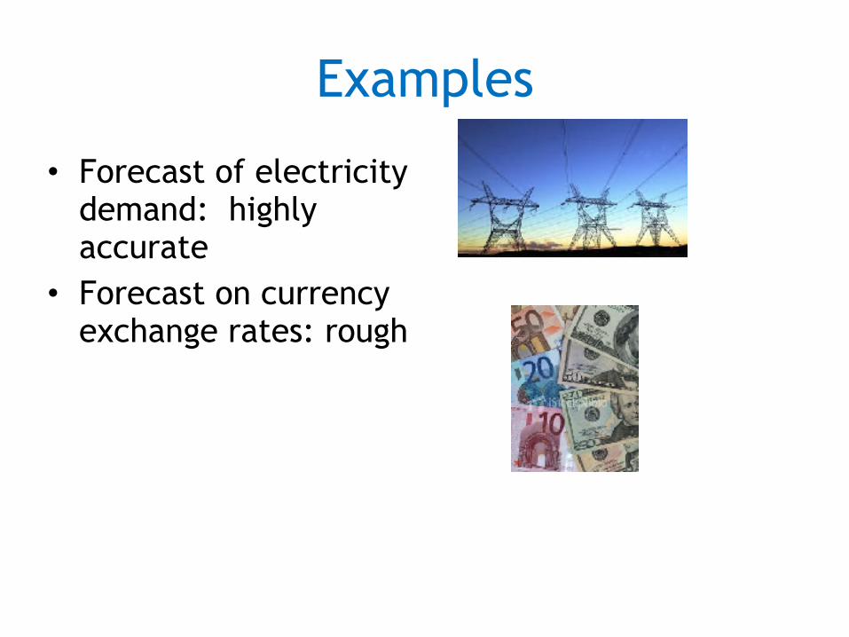
Examples

• Forecast of electricity demand: highly accurate

• Forecast on currency exchange rates: rough

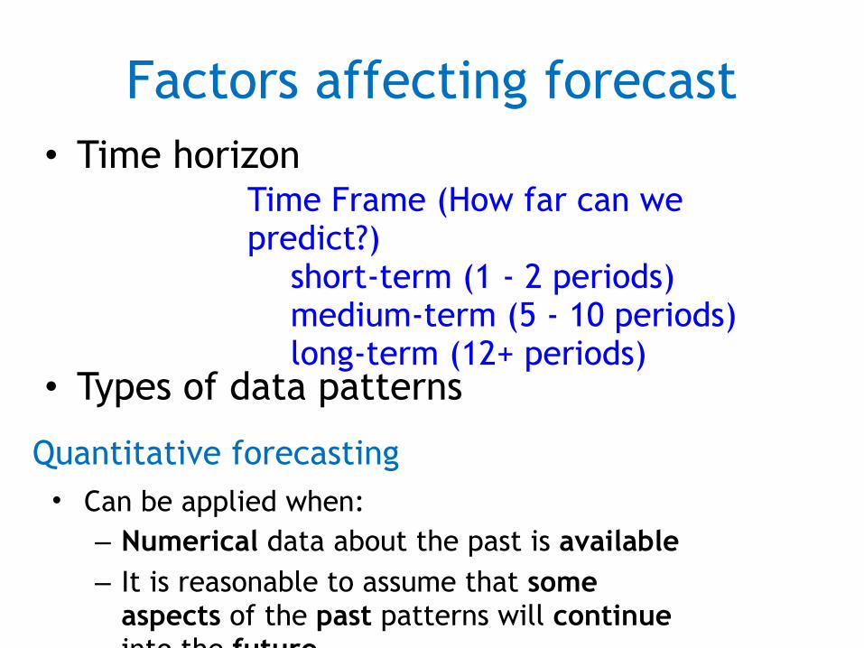
Factors affecting forecast• Time horizon

• Types of data patterns

Time Frame (How far can we predict?)

short-term (1 - 2 periods) medium-term (5 - 10 periods) long-term (12+ periods)

Quantitative forecasting• Can be applied when: – Numerical data about the past is available – It is reasonable to assume that some

aspects of the past patterns will continue into the future

Quantitative forecasting

• Can be applied when: – Numerical data about the past is available – It is reasonable to assume that some aspects of

the past patterns will continue into the future

Time series

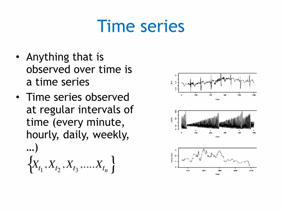
• Anything that is observed over time is a time series

• Time series observed at regular intervals of time (every minute, hourly, daily, weekly, …)

Xt1 ,Xt2 ,Xt3 ,....Xtn{ }

Time series forecasting

• Time series data is useful when you are forecasting something that is changing over time (e.g., stock prices, sales, profits, …)

• Time series forecasting intends to estimate how the sequence of observations will continue in the future

Time Frame (How far can we predict?) short-term (1 - 2 periods) medium-term (5 - 10 periods) long-term (12+ periods)

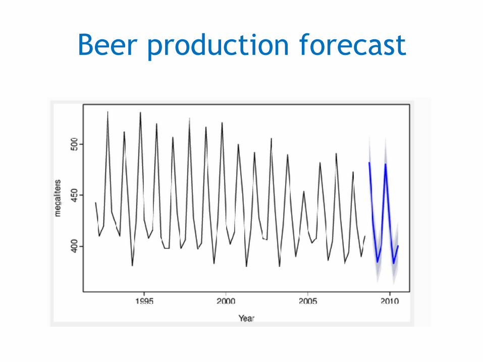
Beer production forecast

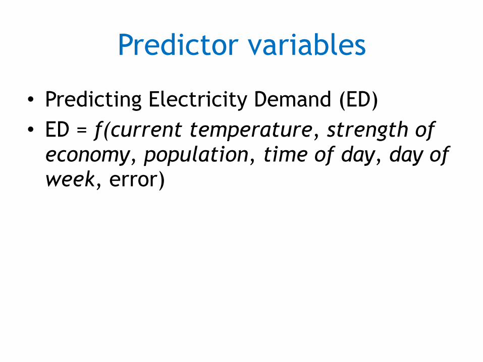
Predictor variables

• Predicting Electricity Demand (ED) • ED = f(current temperature, strength of

economy, population, time of day, day of week, error)

Contents

• Forecasting • Forecaster’s toolbox • Simple regression • Multivariate regression • Time series decomposition • ARIMA models • Advanced forecasting models

Forecasters toolbox

• Graphics • Numerical data summaries • Transformations and adjustments • Evaluating forecast accuracy • Residual diagnostics • Prediction intervals

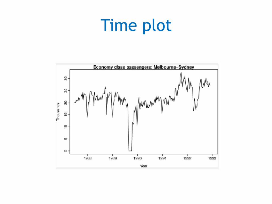
Time plot

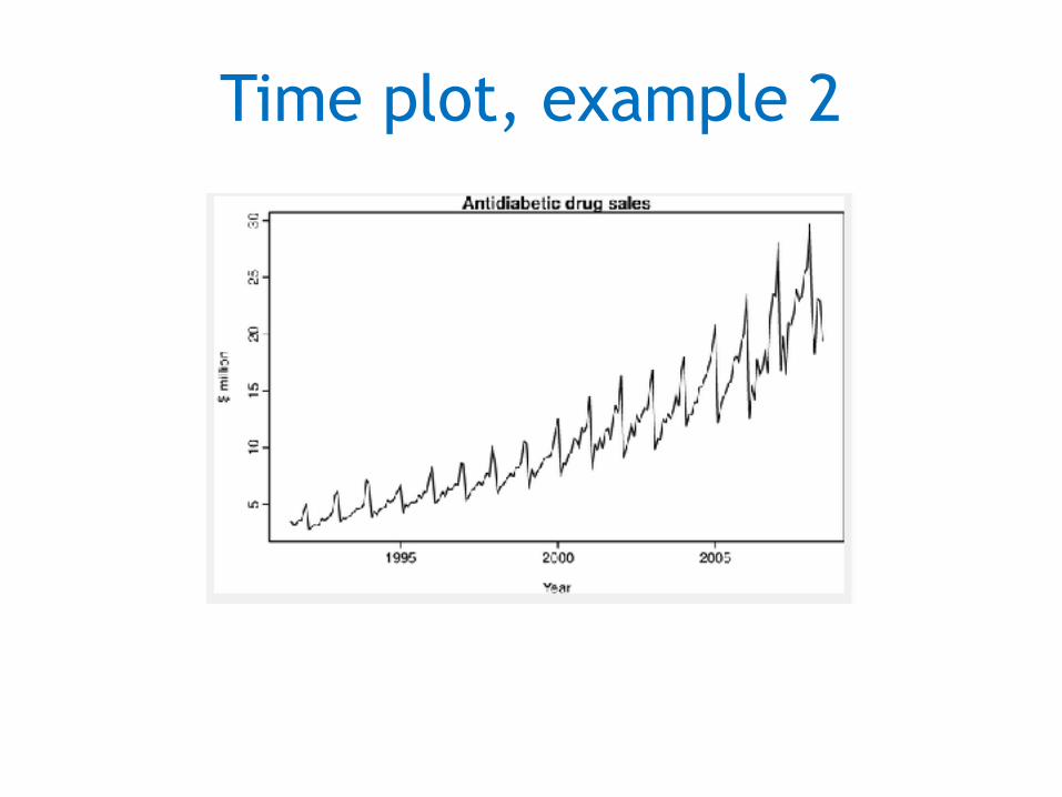
Time plot, example 2

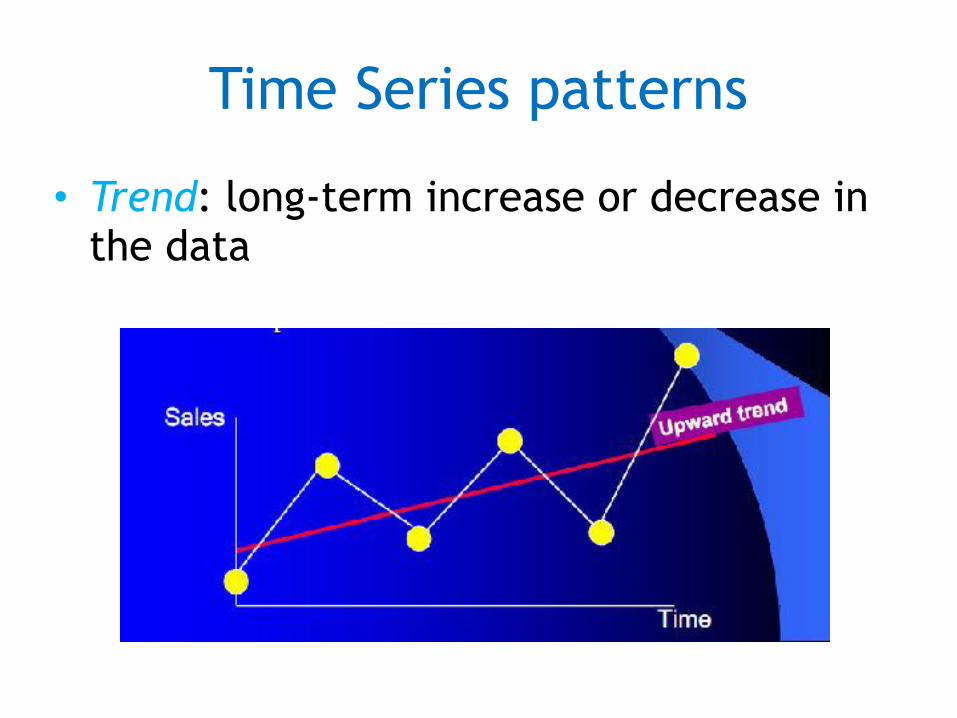
Time Series patterns

• Trend: long-term increase or decrease in the data

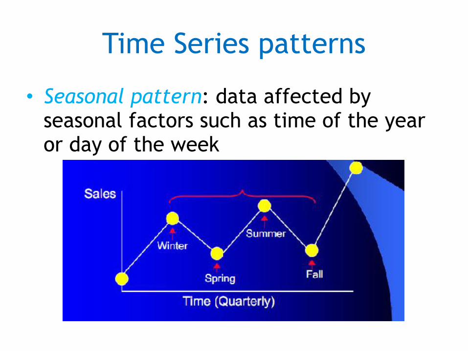
Time Series patterns

• Seasonal pattern: data affected by seasonal factors such as time of the year or day of the week

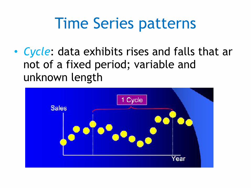
Time Series patterns

• Cycle: data exhibits rises and falls that ar not of a fixed period; variable and unknown length

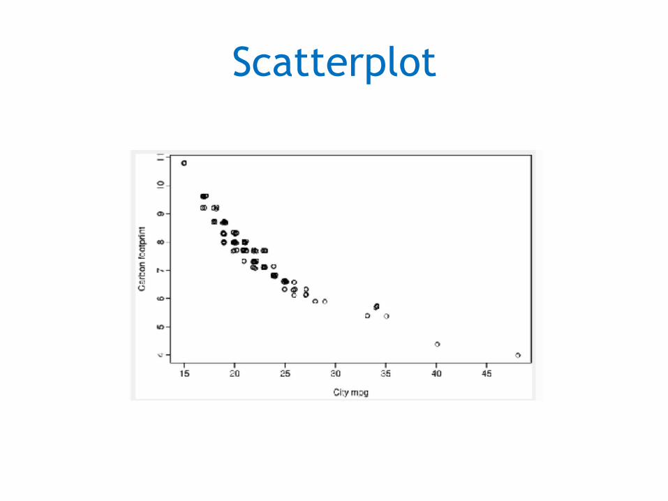
Scatterplot

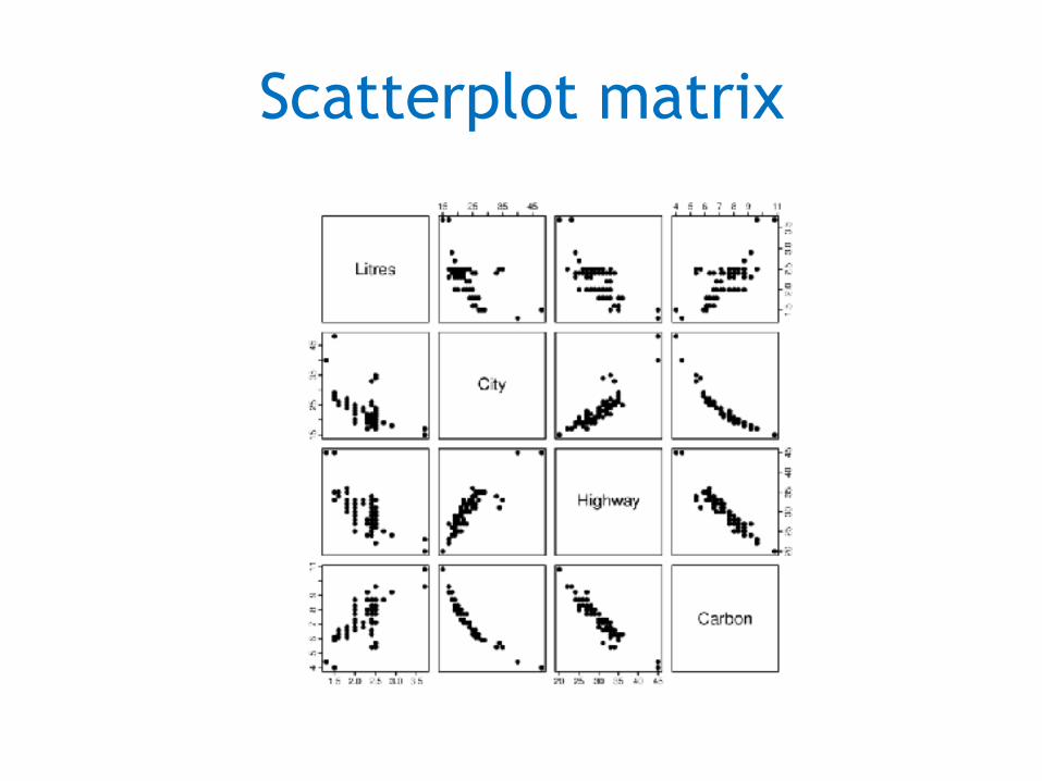
Scatterplot matrix

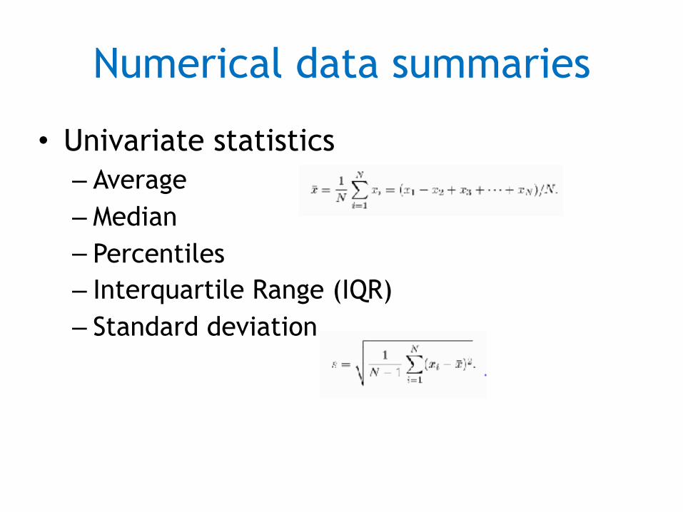
Numerical data summaries

• Univariate statistics – Average – Median – Percentiles – Interquartile Range (IQR) – Standard deviation

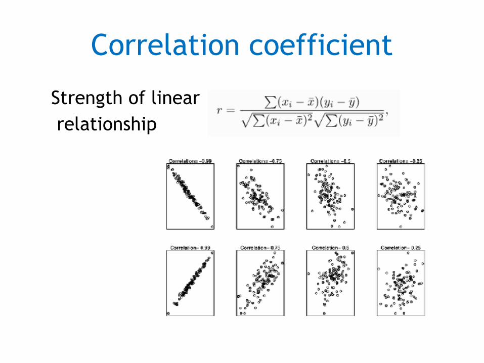
Correlation coefficient

Strength of linear relationship

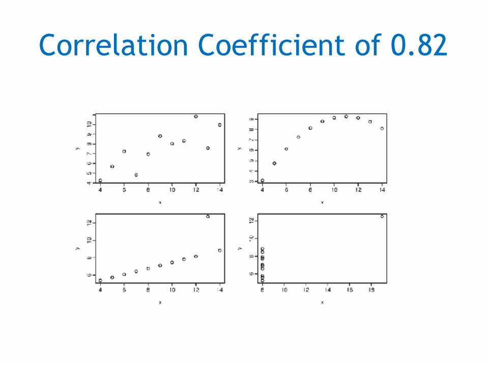
Correlation Coefficient of 0.82

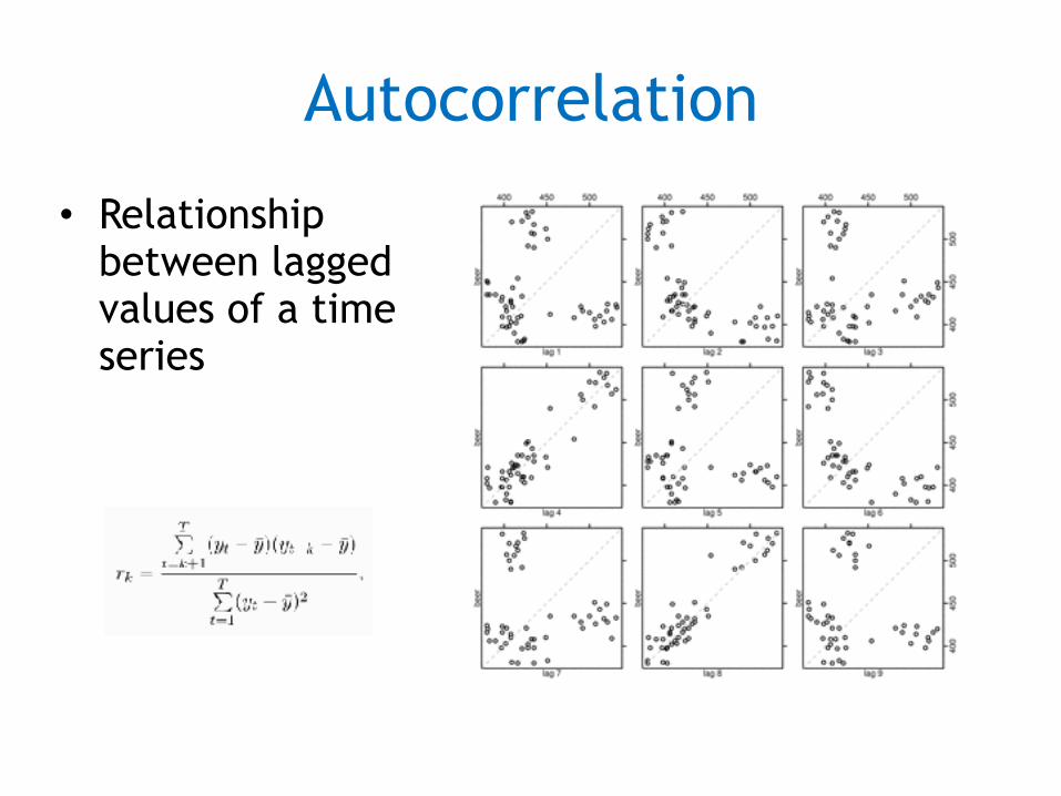
Autocorrelation

• Relationship between lagged values of a time series

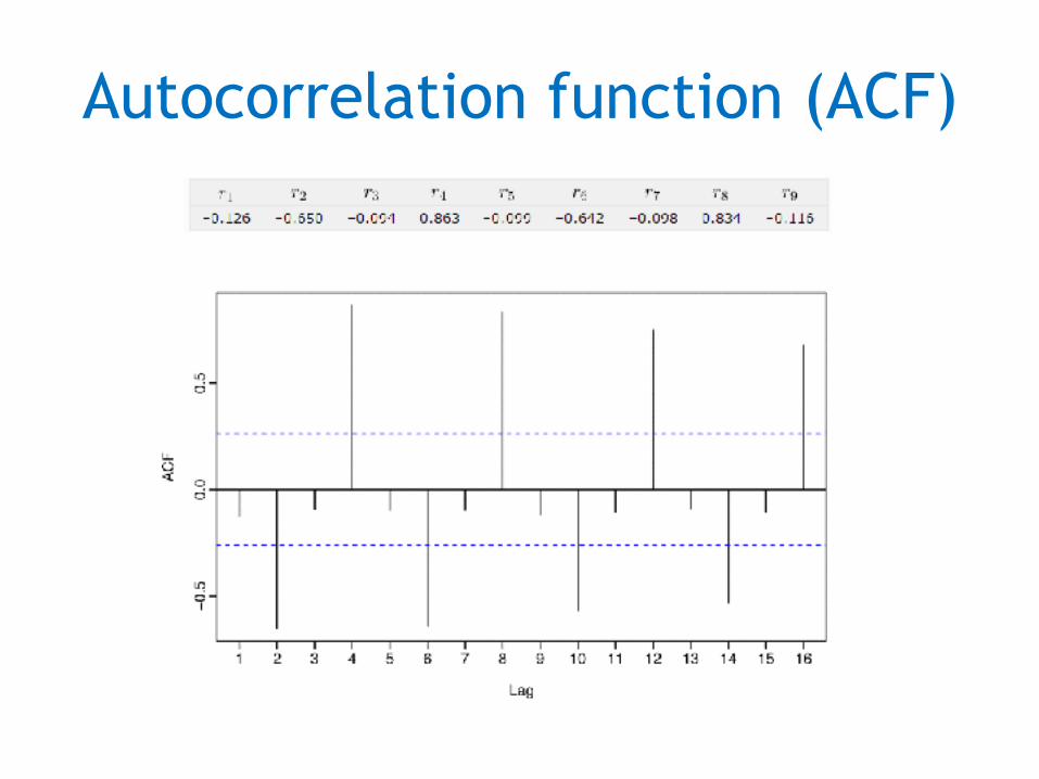
Autocorrelation function (ACF)

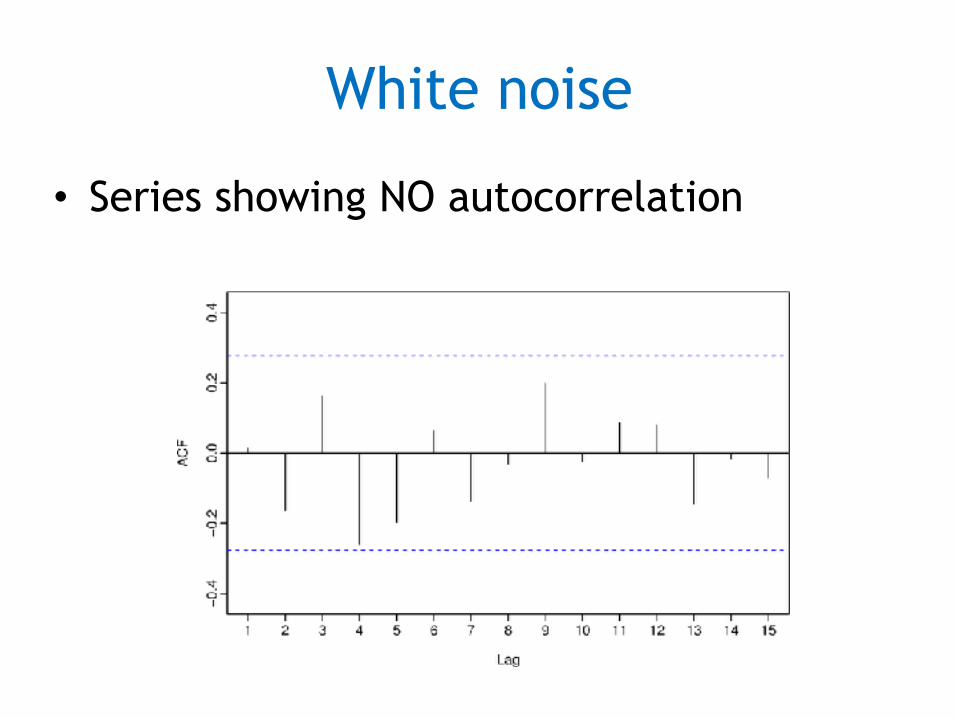
White noise

• Series showing NO autocorrelation

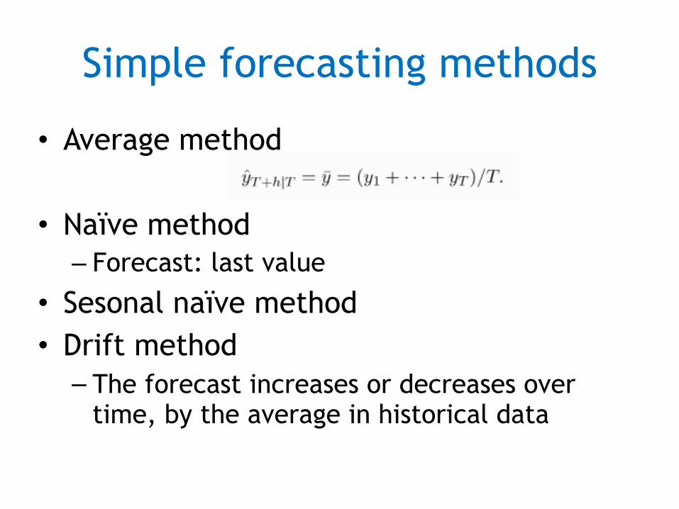
Simple forecasting methods

• Average method

• Naïve method – Forecast: last value

• Sesonal naïve method • Drift method – The forecast increases or decreases over

time, by the average in historical data

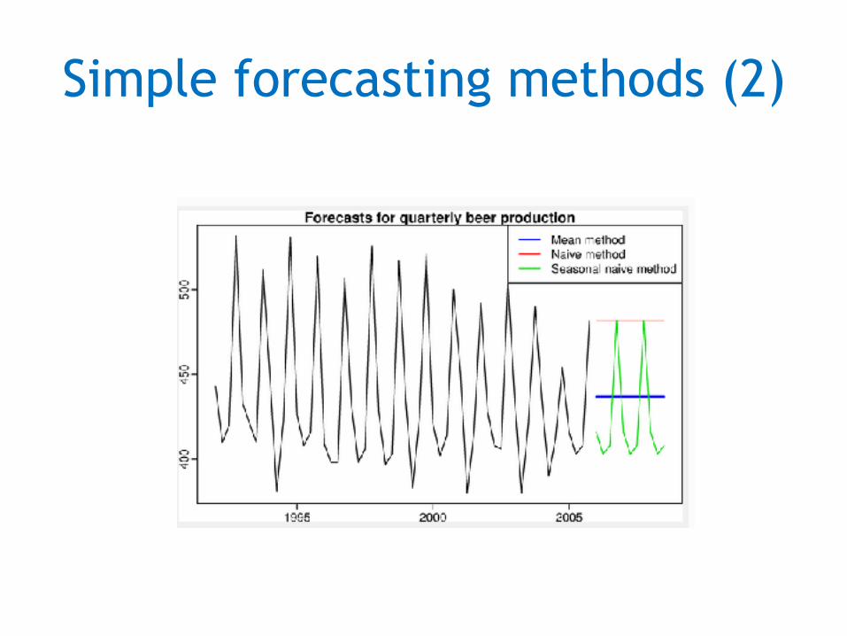
Simple forecasting methods (2)

Transformations

• Adjusting historical data can lead to a simpler forecasting model

• Mathematical transformation • Calendar adjustements • Population adjustements • Inflation adjustements

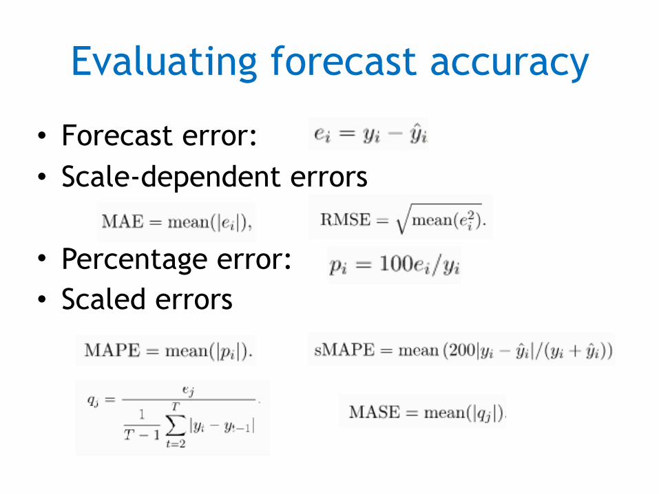
Evaluating forecast accuracy

• Forecast error: • Scale-dependent errors

• Percentage error: • Scaled errors

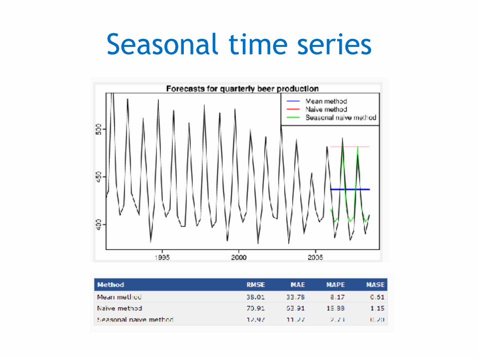
Seasonal time series

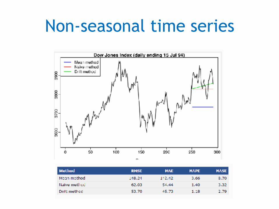
Non-seasonal time series

Methodology

• As in any other modeling task it is essentical to conduct a right evaluation

• Data should be split into training and test parts

• Improved through Cross-validation • Even further improved through Blocked

Cross-Validation

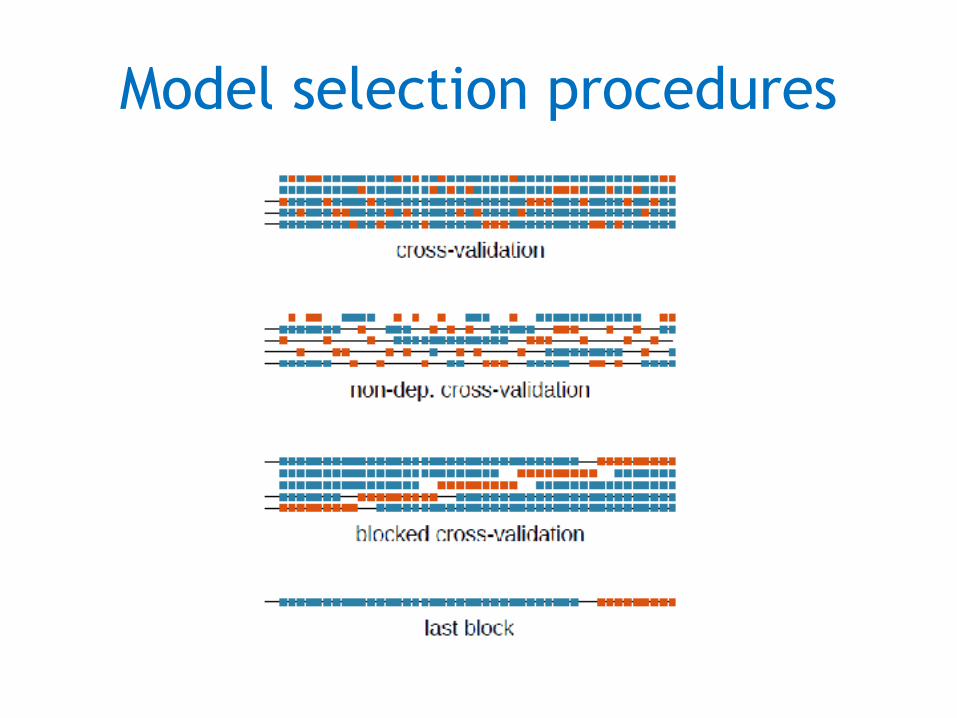
Model selection procedures

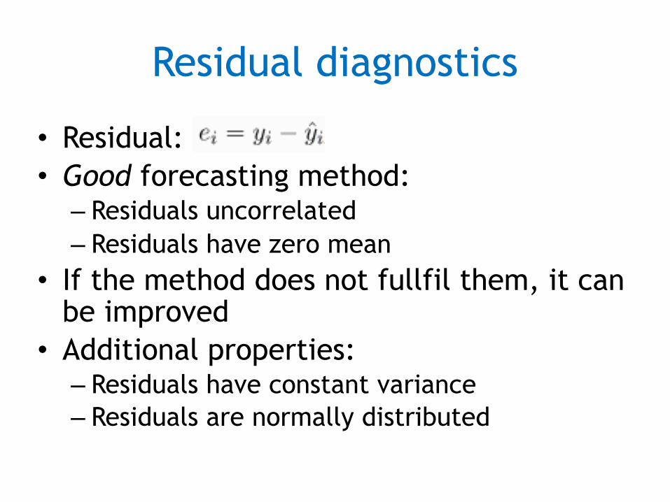
Residual diagnostics

• Residual: • Good forecasting method: – Residuals uncorrelated – Residuals have zero mean

• If the method does not fullfil them, it can be improved

• Additional properties: – Residuals have constant variance – Residuals are normally distributed

Prediction intervals

• A prediction interval gives an interval within the expected value lies with a specified probability

• When forecasting one step-ahead, the standard deviation of the forecast distribution is almost the same as the standard deviation of the residuals

Contents

• Forecasting • Forecaster’s toolbox • Simple regression • Multivariate regression • Time series decomposition • ARIMA models • Advanced forecasting models

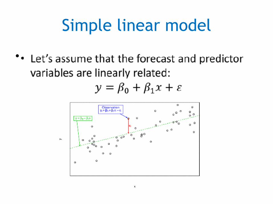
Simple linear model

•  

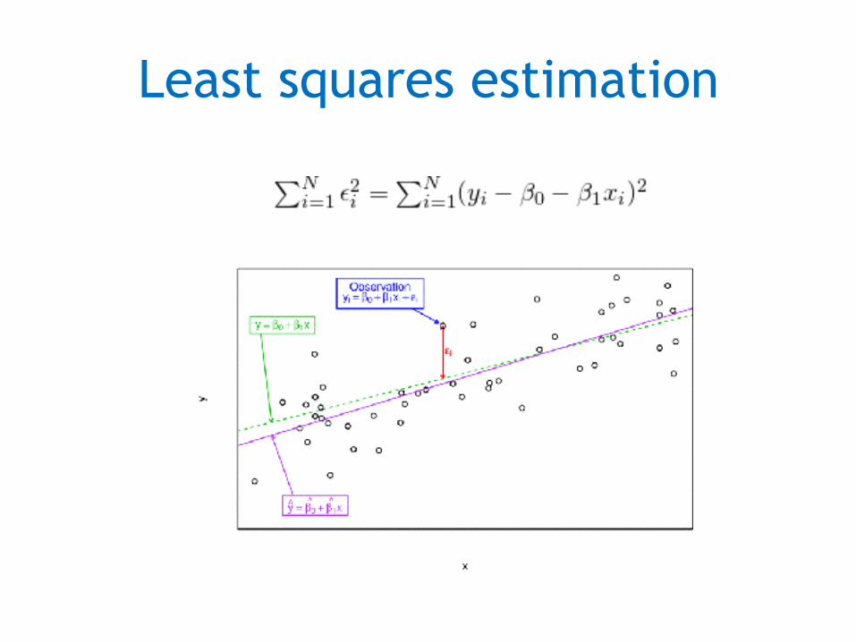
Least squares estimation

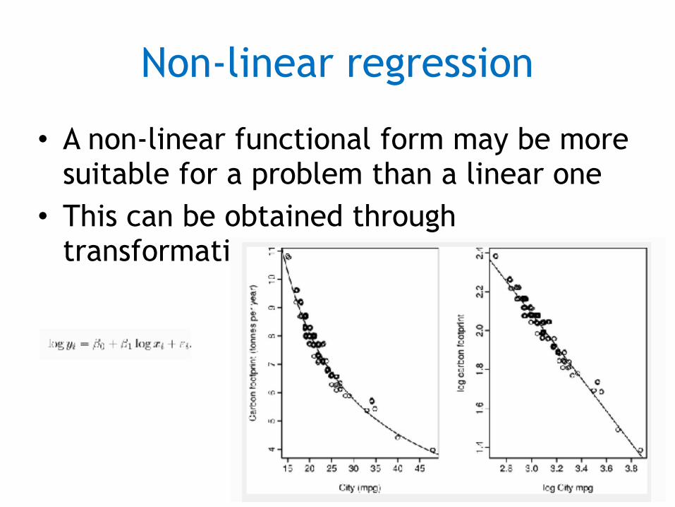
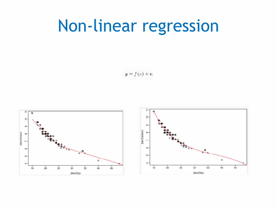
Non-linear regression

• A non-linear functional form may be more suitable for a problem than a linear one

• This can be obtained through transformation of y or x

Contents

• Forecasting • Forecaster’s toolbox • Simple regression • Multivariate regression • Time series decomposition • Exponential smoothing • ARIMA models • Advanced forecasting models

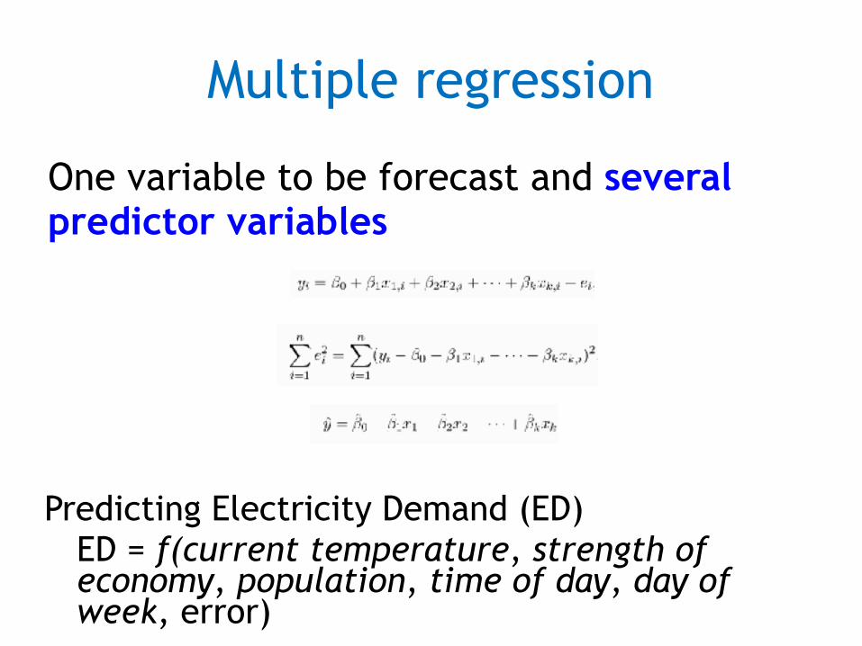
Multiple regression

One variable to be forecast and several predictor variables

Predicting Electricity Demand (ED)

ED = f(current temperature, strength of economy, population, time of day, day of week, error)

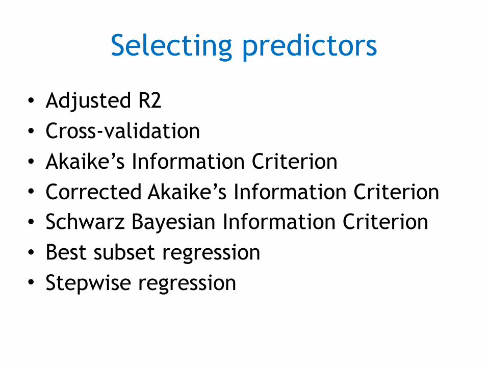
Selecting predictors

• Adjusted R2 • Cross-validation • Akaike’s Information Criterion • Corrected Akaike’s Information Criterion • Schwarz Bayesian Information Criterion • Best subset regression • Stepwise regression

Non-linear regression

Correlation is not causation

• A variable x may be useful for predicting a variable y, but that does not mean x is causing y.

• Correlations are useful for forecasting, even when there is no causal relationship between the two variables

Contents

• Forecasting • Forecaster’s toolbox • Simple regression • Multivariate regression • Time series decomposition • ARIMA models • Advanced forecasting models

Time Series decomposition

• Time series can exhibit a huge variety of patterns and it is helpful to categorize some of the patterns and behaviors that can be seen

• It is also sometimes useful to try to split a time series into several components, each representing one of the underlying components

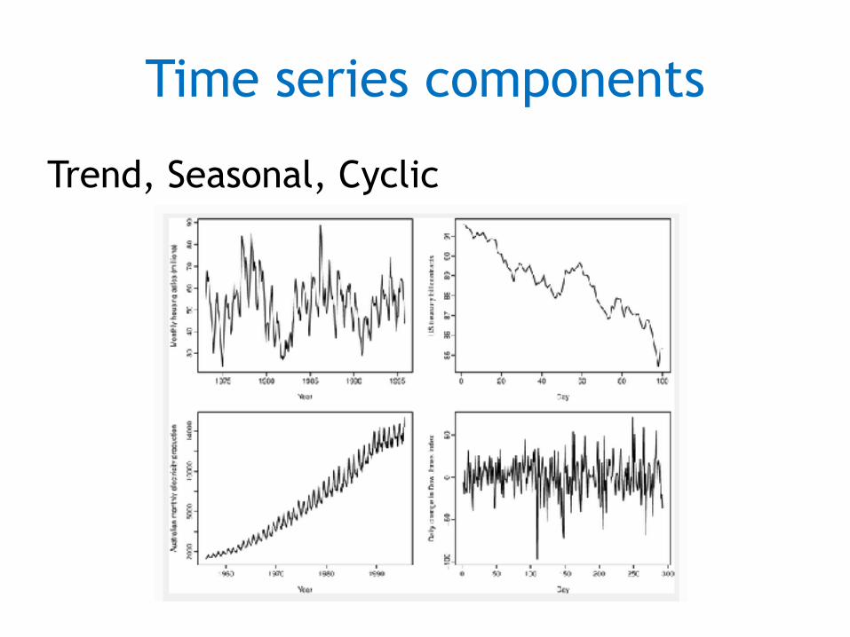
Time series components

Trend, Seasonal, Cyclic

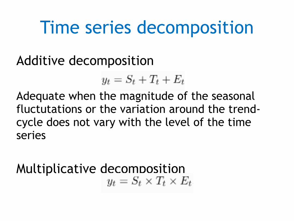
Time series decomposition

Additive decomposition

Adequate when the magnitude of the seasonal fluctutations or the variation around the trend-cycle does not vary with the level of the time series

Multiplicative decomposition

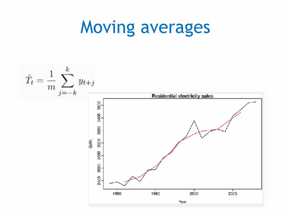
Moving averages

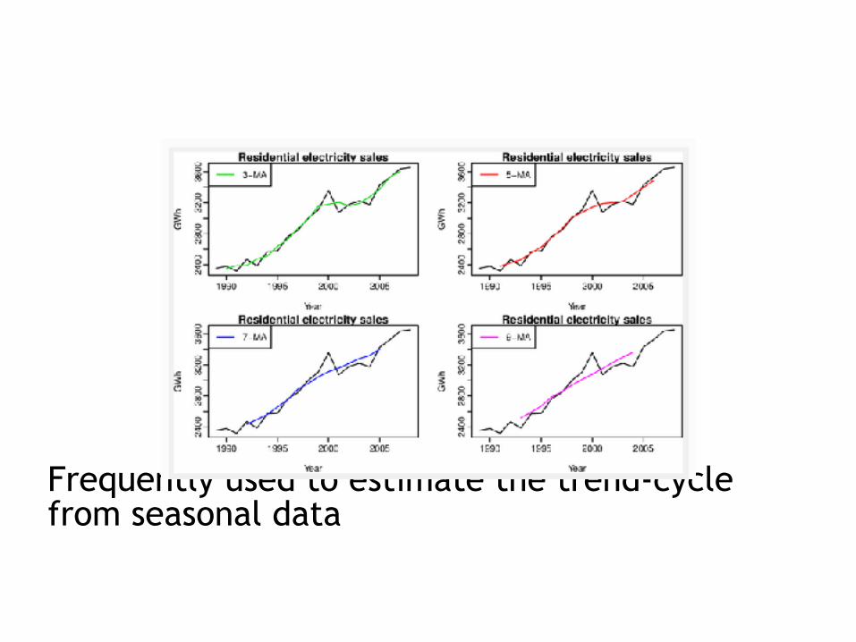
Frequently used to estimate the trend-cycle from seasonal data

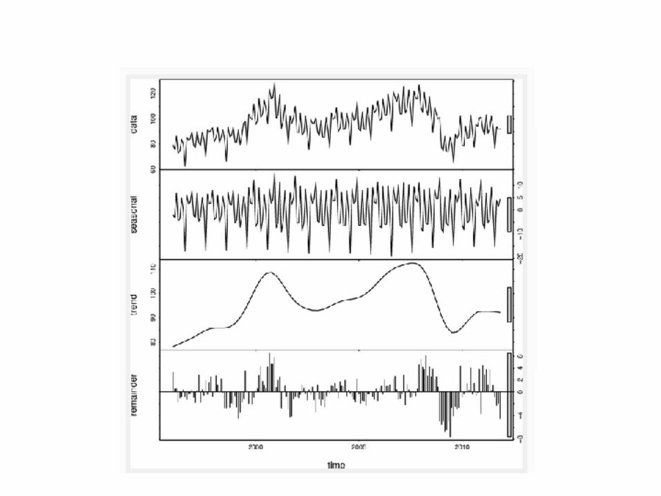
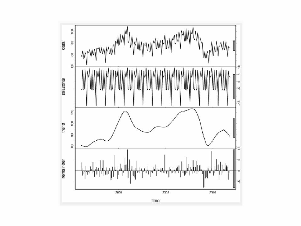
STL decomposition

• STL is a robust and versatil decomposition method: Seasonal and Trend decomposition using Loess. – It can handle any type of seasonality – The seasonal component is allowed to change

over time, within a range controllable by the user

– The smoothness of the trend-cycle can also be controlled by the user

– It is robust to outliers

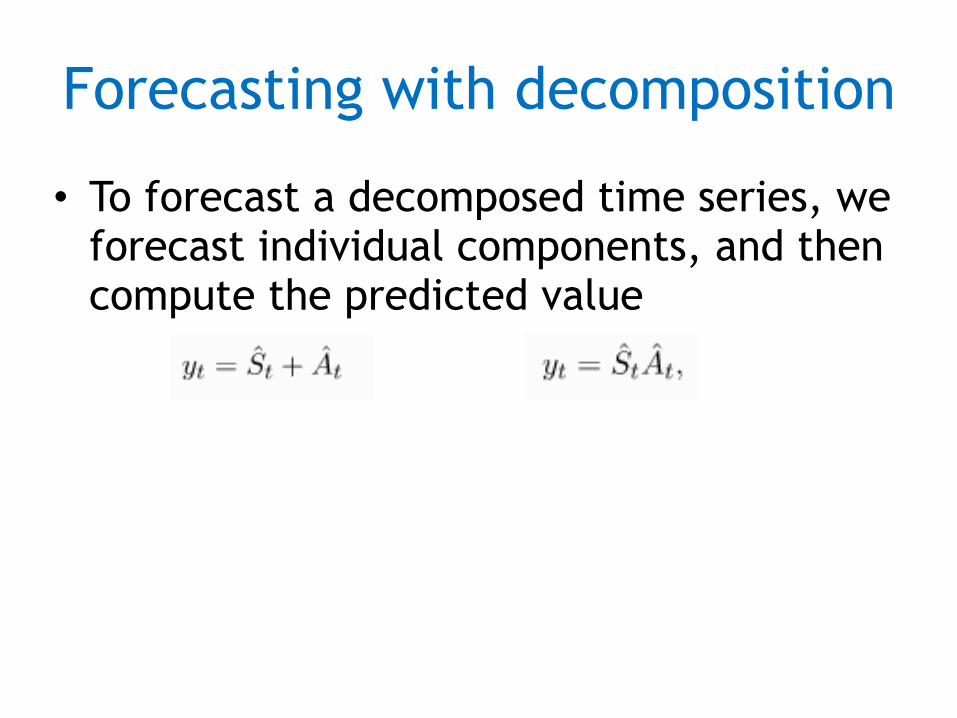
Forecasting with decomposition

• To forecast a decomposed time series, we forecast individual components, and then compute the predicted value

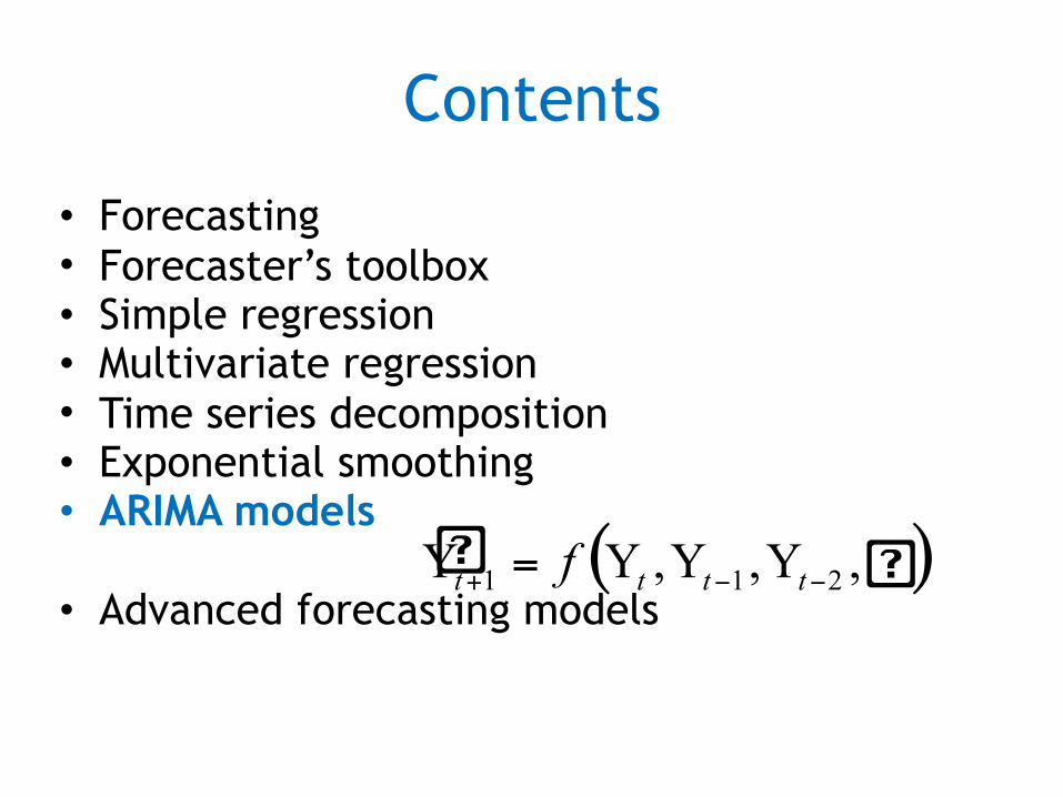
Contents

• Forecasting • Forecaster’s toolbox • Simple regression • Multivariate regression • Time series decomposition • Exponential smoothing • ARIMA models

• Advanced forecasting models( )� , , ,Y Y Y Yt t t tf+ − −=1 1 2 �

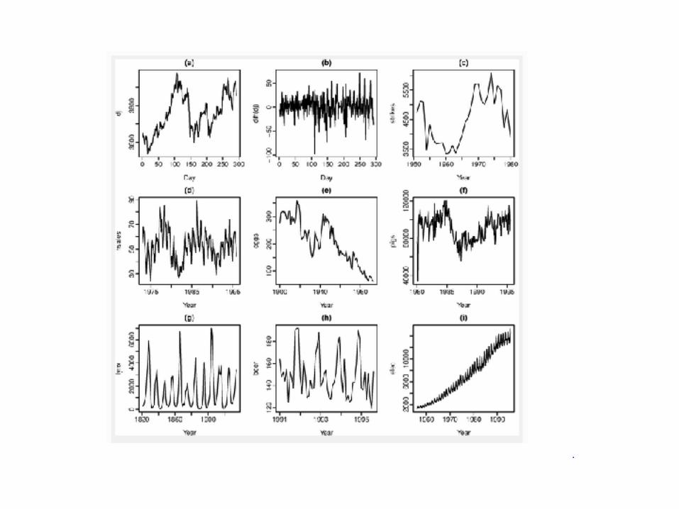
Stationarity

• A stationary time series is one whose properties do not depend on the time at which the series is observed

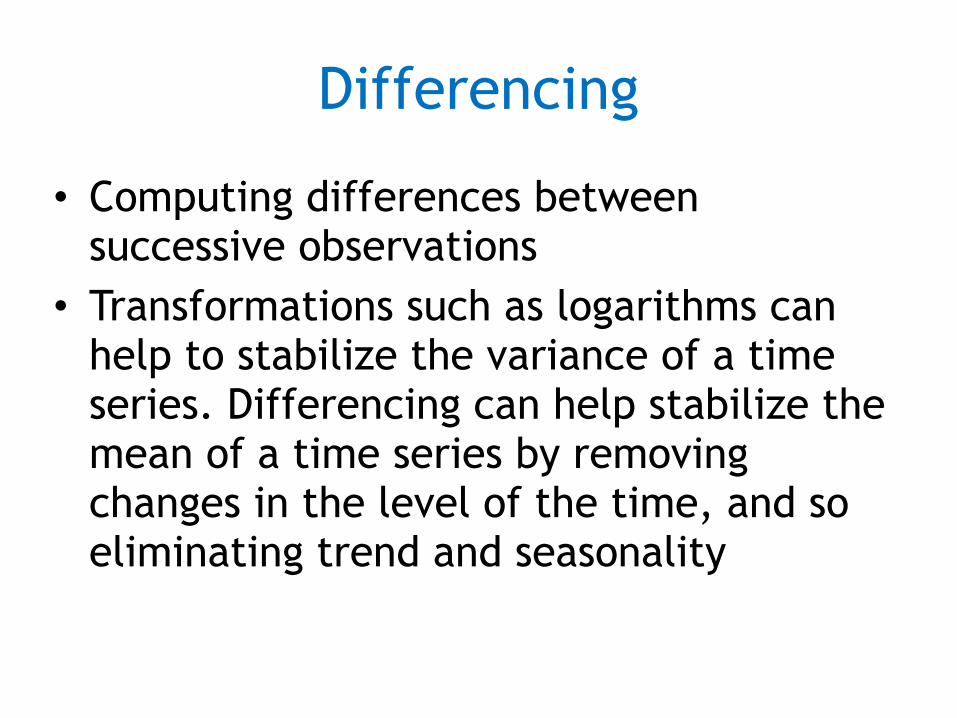
Differencing

• Computing differences between successive observations

• Transformations such as logarithms can help to stabilize the variance of a time series. Differencing can help stabilize the mean of a time series by removing changes in the level of the time, and so eliminating trend and seasonality

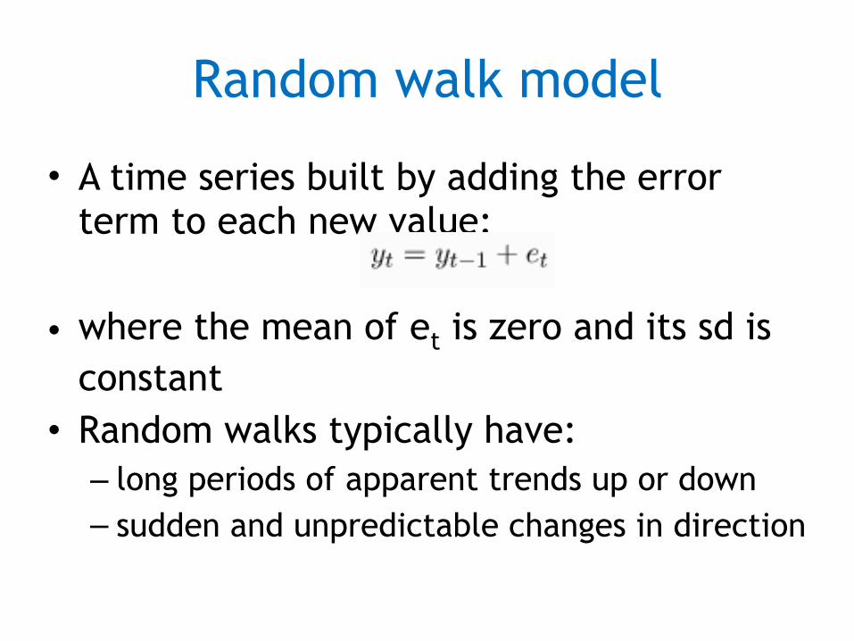
Random walk model

• A time series built by adding the error term to each new value:

• where the mean of et is zero and its sd is constant

• Random walks typically have: – long periods of apparent trends up or down – sudden and unpredictable changes in direction

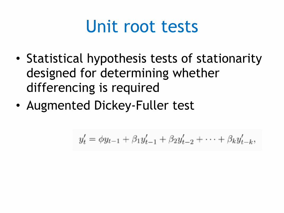
Unit root tests

• Statistical hypothesis tests of stationarity designed for determining whether differencing is required

• Augmented Dickey-Fuller test

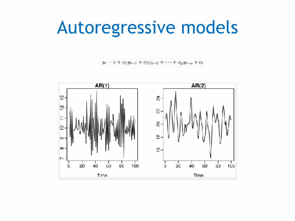
Autoregressive models

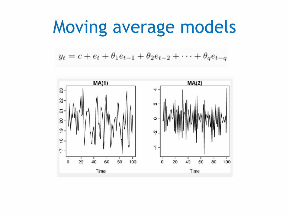
Moving average models

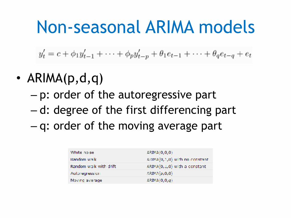
Non-seasonal ARIMA models

• ARIMA(p,d,q) – p: order of the autoregressive part – d: degree of the first differencing part – q: order of the moving average part

Neural networks

• Multilayered perceptrons • RBF • Recurrent neural networks

MLP

• Multilayered Perceptrons are the best known and widely used model of Neural Networks

• Due to their performance in regression problems they are frequently applied to time series forecasting

• The same consideration applied when addressing a regular regression problem are taken when approaching time series analysis and forecasting

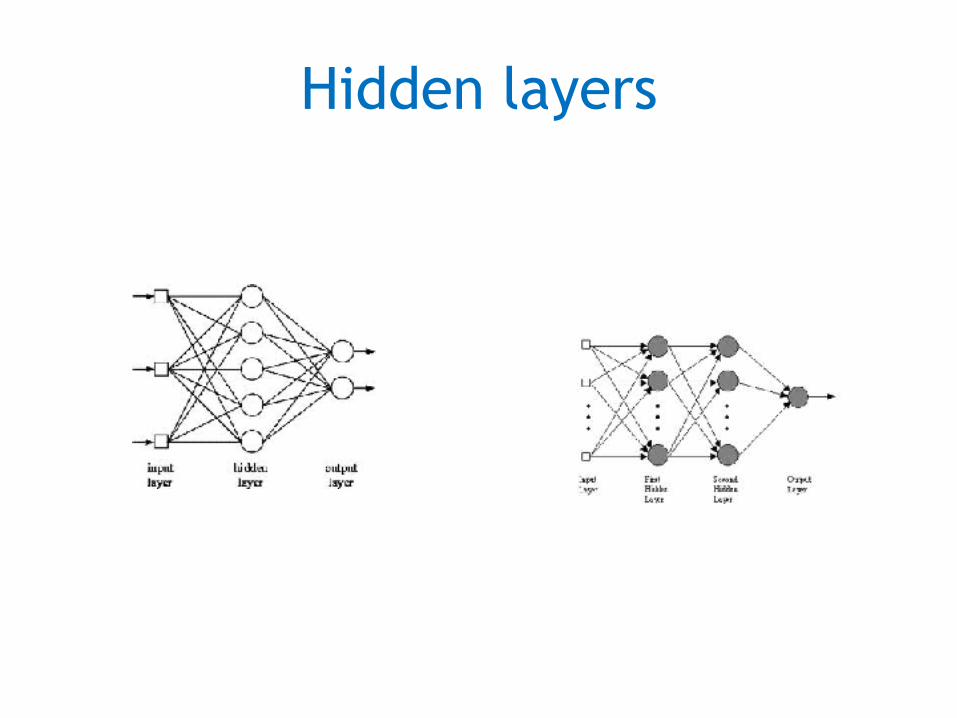
Hidden layers

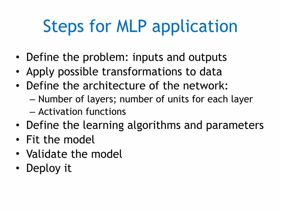
Steps for MLP application

• Define the problem: inputs and outputs • Apply possible transformations to data • Define the architecture of the network: – Number of layers; number of units for each layer – Activation functions

• Define the learning algorithms and parameters • Fit the model • Validate the model • Deploy it

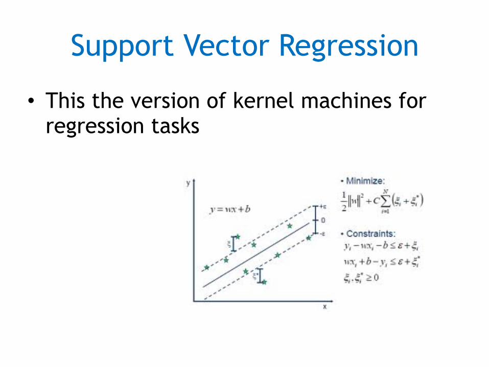
Support Vector Regression

• This the version of kernel machines for regression tasks

References

• C. Chatfield, «The analysis of time series: An Introduction», Chapman & Hall/CRC, 2003

• J.D. Hamilton, «Time Series Analysis», Princeton University Press, 1994

• R. Hyndman, G. Athanasopoulus, «Forecasting and time series» 2013

• P.J. Brockwell, R.A. Davis, «Time Series: Theory and Methods», 2nd Ed., Springer, 1991

• J.S. Armstrong (ed), «Principles of Forecasting: A Handbook for Researchers and Practitioners», Springer, 2001

• S.G. Makridakis, S.C. Wheelwright, R.J. Hyndman, «Forecasting», 3rd Ed., Wiley & Sons, 1998

• P.J. Brockwell, R.A. Davis, «Introdution to Time Series and Forecasting», 2nd ed., Springer, 2002

• A.K.Palit, D. Popovic, «Computational Intelligence in Time Series Forecasting: Theory and Engineering Applications», Springer, 2005

• R.H. Shumway, D.S. Stoffer, «Time Series Analysis and Its Applications», Springer, 2nd Ed., 2006

References

INTELIGENCIA DE NEGOCIO 2016 - 2017

■ Tema 1. Introducción a la Inteligencia de Negocio ■ Tema 2. Minería de Datos. Ciencia de Datos ■ Tema 3. Modelos de Predicción: Clasificación, regresión

y series temporales ■ Tema 4. Preparación de Datos ■ Tema 5. Modelos de Agrupamiento o Segmentación ■ Tema 6. Modelos de Asociación ■ Tema 7. Modelos Avanzados de Minería de Datos. ■ Tema 8. Big Data