MATEMATIKA DIKSKRITMATEMATIKA DIKSKRIT Drs. Daflk, M.Sc, Ph.D Fakultas Keguruan dan Ilmu Pendidikan...
51
MATEMATIKA DIKSKRIT Drs. Dafik, M.Sc, Ph.D Fakultas Keguruan dan Ilmu Pendidikan Universitas Jember Juli 2010
Transcript of MATEMATIKA DIKSKRITMATEMATIKA DIKSKRIT Drs. Daflk, M.Sc, Ph.D Fakultas Keguruan dan Ilmu Pendidikan...
MATEMATIKA
DIKSKRIT
Drs. Dafik, M.Sc, Ph.D
Fakultas Keguruan dan Ilmu Pendidikan
Universitas Jember
Juli 2010

Contents
Contents iii
List of Tables iv
List of Figures vii
INTRODUCTION 1
1 Basic Terminology 1
1.1 Undirected graphs . . . . . . . . . . . . . . . . . . . . . . . . . . 1
1.2 Directed graphs . . . . . . . . . . . . . . . . . . . . . . . . . . . . 5
1.3 Exercises 1 . . . . . . . . . . . . . . . . . . . . . . . . . . . . . . . 8
2 Some Applications of Graphs 12
2.1 Applications of Graphs . . . . . . . . . . . . . . . . . . . . . . . . 12
2.2 Classifying Problems . . . . . . . . . . . . . . . . . . . . . . . . . 19
2.3 Exercises 2 . . . . . . . . . . . . . . . . . . . . . . . . . . . . . . . 20
3 Planarity of Graph 23
ii
CONTENTS iii
3.1 Planar Graph . . . . . . . . . . . . . . . . . . . . . . . . . . . . . 23
3.2 Euler’s Formula . . . . . . . . . . . . . . . . . . . . . . . . . . . . 24
3.3 Cycle Method for Planarity Testing . . . . . . . . . . . . . . . . . 28
3.4 Kuratowski’s Theorem . . . . . . . . . . . . . . . . . . . . . . . . 28
3.5 Duality . . . . . . . . . . . . . . . . . . . . . . . . . . . . . . . . . 29
3.6 Convex Polyhedra . . . . . . . . . . . . . . . . . . . . . . . . . . . 30
3.7 Exercises 3 . . . . . . . . . . . . . . . . . . . . . . . . . . . . . . . 31
4 Construction Techniques 32
4.1 Generalised de Bruijn and Kautz Digraphs . . . . . . . . . . . . . 33
4.2 Line Digraphs and Partial Line Digraphs . . . . . . . . . . . . . . 34
4.3 Generalised de Bruijn and Kautz Digraphs on Alphabets . . . . . 36
4.4 Voltage Assignments . . . . . . . . . . . . . . . . . . . . . . . . . 37
4.5 Digon Reduction and Vertex Deletion Scheme . . . . . . . . . . . 40
4.6 Exercises 4 . . . . . . . . . . . . . . . . . . . . . . . . . . . . . . . 43
List of Tables
3.1 The plane drawing of G with its relevant properties of G∗. . . . . 30
4.1 The list of voltage assignment values for given k and 3 ≤ n ≤ 18,
base digraph and group Γ. . . . . . . . . . . . . . . . . . . . . . . 39
4.2 Range of orders n when minimum diameter is achieved by different
techniques. . . . . . . . . . . . . . . . . . . . . . . . . . . . . . . . 43
iv
List of Figures
1.1 Example of a graph with isolated vertex. . . . . . . . . . . . . . . 2
1.2 Example of a graph . . . . . . . . . . . . . . . . . . . . . . . . . . 2
1.3 Graph and three of its subgraphs . . . . . . . . . . . . . . . . . . 3
1.4 Isomorphism in graphs . . . . . . . . . . . . . . . . . . . . . . . . 4
1.5 Graph and its adjacency matrix . . . . . . . . . . . . . . . . . . . 5
1.6 Diregular and non-diregular digraphs. . . . . . . . . . . . . . . . . 6
1.7 Isomorphism in digraphs. . . . . . . . . . . . . . . . . . . . . . . . 7
1.8 Digraph and its adjacency matrix. . . . . . . . . . . . . . . . . . . 8
1.9 Connected graph. . . . . . . . . . . . . . . . . . . . . . . . . . . . 9
1.10 Petersen graph. . . . . . . . . . . . . . . . . . . . . . . . . . . . . 9
1.11 Isomorphism in digraphs. . . . . . . . . . . . . . . . . . . . . . . . 10
1.12 Digraph and its subdigraph. . . . . . . . . . . . . . . . . . . . . . 10
1.13 Two connected digraphs. . . . . . . . . . . . . . . . . . . . . . . . 11
2.1 Alkane compound: Metane, Etane and Propane. . . . . . . . . . . 13
2.2 Konigsberg city. . . . . . . . . . . . . . . . . . . . . . . . . . . . . 14
2.3 The Konigsberg bridge. . . . . . . . . . . . . . . . . . . . . . . . . 14
v
LIST OF FIGURES vi
2.4 A road map of cities in USA. . . . . . . . . . . . . . . . . . . . . 15
2.5 An example of utilities problem. . . . . . . . . . . . . . . . . . . . 15
2.6 Portion of a printed circuit. . . . . . . . . . . . . . . . . . . . . . 16
2.7 Network topologies. . . . . . . . . . . . . . . . . . . . . . . . . . . 17
2.8 Combination of network topologies. . . . . . . . . . . . . . . . . . 17
2.9 World wide web network topology. . . . . . . . . . . . . . . . . . 18
2.10 Map of Jember. . . . . . . . . . . . . . . . . . . . . . . . . . . . . 20
2.11 Some examples of planar graph. . . . . . . . . . . . . . . . . . . . 21
2.12 Two examples of undirected graph. . . . . . . . . . . . . . . . . . 21
2.13 Three examples of directed graph. . . . . . . . . . . . . . . . . . . 22
3.1 The graph with its planar graph . . . . . . . . . . . . . . . . . . . 23
3.2 The graph K3,3 and K5 are non planar . . . . . . . . . . . . . . . 24
3.3 The plane drawing of graph G with their faces . . . . . . . . . . . 25
3.4 The plane drawing of planar graph . . . . . . . . . . . . . . . . . 26
3.5 The plane drawing of planar graph . . . . . . . . . . . . . . . . . 29
3.6 A simple connected graph with its subdivision . . . . . . . . . . . 29
3.7 The plane drawing of planar graphs G with its dual graphs G∗ . . 29
4.1 Generalised de Bruijn digraphs G ∈ G(9, 3, 2). . . . . . . . . . . . 34
4.2 Generalised Kautz digraphs G ∈ G(9, 2, 3). . . . . . . . . . . . . . 34
4.3 Digraphs G ∈ G(3, 2, 1) with its line digraphs L(G) ∈ G(6, 2, 2)
and L2(G) ∈ G(12, 2, 3). . . . . . . . . . . . . . . . . . . . . . . . 35
4.4 Digraph G and one of its partial line digraphs. . . . . . . . . . . . 36
LIST OF FIGURES vii
4.5 Example of generalised Kautz digraph on alphabet. . . . . . . . . 38
4.6 Digraph G and its lift Gα. . . . . . . . . . . . . . . . . . . . . . . 40
4.7 The base digraphs. . . . . . . . . . . . . . . . . . . . . . . . . . . 41
4.8 Digraphs G ∈ G(12, 2, 3) and G′ ∈ G(11, 2, 3). . . . . . . . . . . . . 42
4.9 Digraph G ∈ G(12, 2, 3) and G1 ∈ G(11, 2, 3) obtained from G. . . 42

Modul 1
Basic Terminology
1.1 Undirected graphs
By an undirected graph, or a graph, we mean a structure G = (V (G), E(G)),
where V (G) is a finite nonempty set of elements called vertices, and E(G) is a
set (possibly empty) of unordered pairs u, v of vertices u, v ∈ V (G), called
edges. The number of vertices of a graph G is the order of G, commonly denoted
by |V (G)|. The number of edges is the size of G, often denoted by |E(G)|. A
graph G that has order p = |V (G)| and size q = |E(G)| is sometimes called a
(p, q)-graph.
Let u, v ∈ V (G). Vertex u is said to be adjacent to v if there is an edge e between
u and v, that is, e = uv. Vertex v is then called a neighbour of u, or we say that u
and v are incident with edge e. For example, in Figure 1.1, vertex v1 is adjacent
to vertex v4; vertex v4 is incident with edges v4v5 and v4v6; and the neighbours
of vertex v4 are v1, v3, v5 and v6.
The number of neighbours of v is called the degree of a vertex v of G. If a vertex
v has degree 0, that is, v is not adjacent to any other vertex, then v is called an
isolated vertex. A vertex of degree 1 is called an end vertex, or a leaf. The degree
1
Chapter 1. Basic Terminology 2
v7
v4
v1 v2 v3
v6v5
Figure 1.1: Example of a graph with isolated vertex.
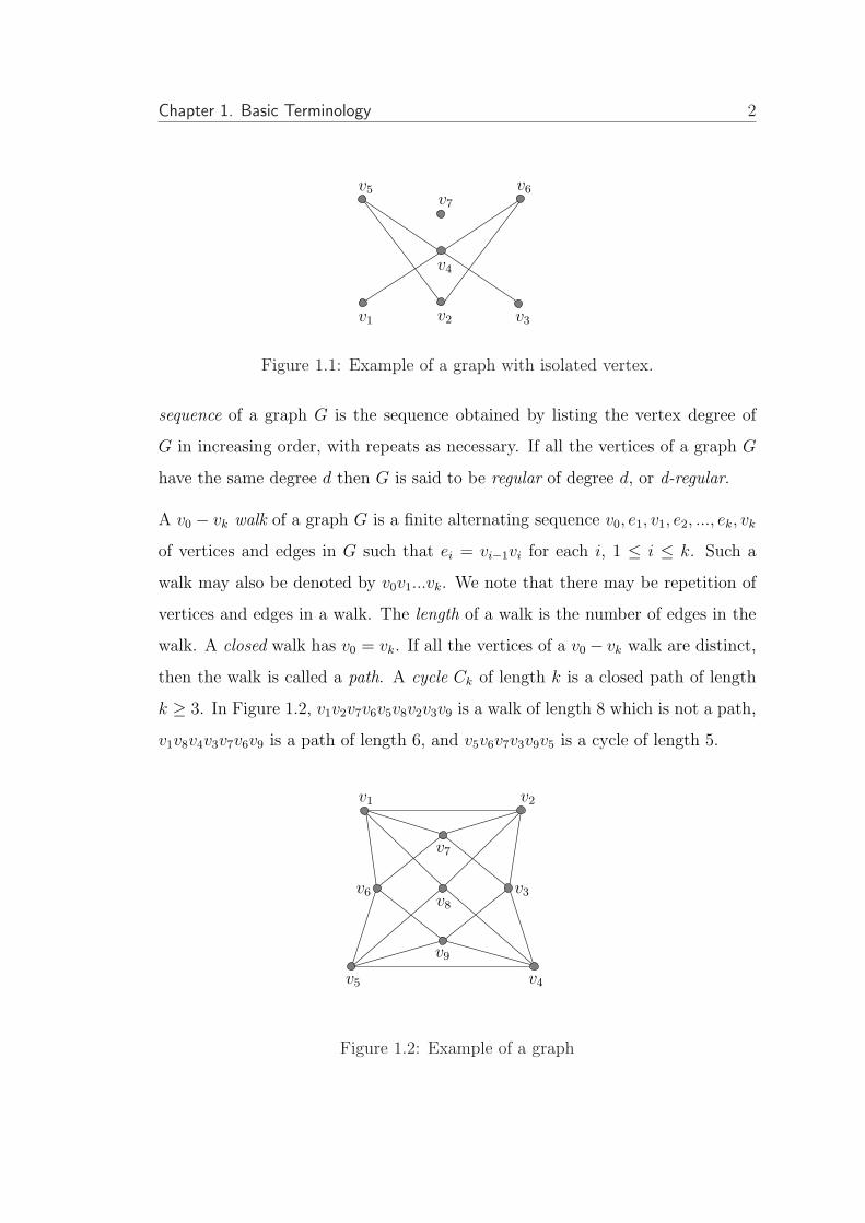
sequence of a graph G is the sequence obtained by listing the vertex degree of
G in increasing order, with repeats as necessary. If all the vertices of a graph G
have the same degree d then G is said to be regular of degree d, or d-regular.
A v0 − vk walk of a graph G is a finite alternating sequence v0, e1, v1, e2, ..., ek, vk
of vertices and edges in G such that ei = vi−1vi for each i, 1 ≤ i ≤ k. Such a
walk may also be denoted by v0v1...vk. We note that there may be repetition of
vertices and edges in a walk. The length of a walk is the number of edges in the
walk. A closed walk has v0 = vk. If all the vertices of a v0 − vk walk are distinct,
then the walk is called a path. A cycle Ck of length k is a closed path of length
k ≥ 3. In Figure 1.2, v1v2v7v6v5v8v2v3v9 is a walk of length 8 which is not a path,
v1v8v4v3v7v6v9 is a path of length 6, and v5v6v7v3v9v5 is a cycle of length 5.
v1
v8
v7
v9
v3v6
v5 v4
v2
Figure 1.2: Example of a graph

Chapter 1. Basic Terminology 3
The distance from vertex u to v, denoted by δ(u, v), is the length of a shortest
path from vertex u to vertex v. For any vertices u, v, w in G, we have δ(u,w) ≤δ(u, v)+δ(v, w) and if δ(u, v) ≥ 2 then there is a vertex z in G such that δ(u, v) =
δ(u, z) + δ(z, v). For example, the distance from vertex v1 to v4 of the graph in
Figure 1.2 is 2. The eccentricity of v, denoted by e(v), is defined by e(v) =
maxδ(u, v) : u ∈ V, u 6= v and the radius of G, denoted by rad G, is defined by
rad G = mine(v) : v ∈ V . The diameter of a graph G is the longest distance
between any two vertices in G and is denoted diam G = maxe(v) : v ∈ V and
the girth of a graph G is the length of the shortest cycle in G. For example, the
graph in Figure 1.2 has diameter 2 and girth 3.
A graph H is a subgraph of G if every vertex of H is a vertex of G, and every
edge of H is an edge of G. In other words, V (H) ⊂ V (G) and E(H) ⊂ E(G).
We say that a subgraph H is a spanning subgraph of G if H contains all the
vertices of G. Let F be a nonempty subset of the vertex set V (G). The induced
subgraph G[F ] is a subgraph of G consisting of the vertex-set F together with all
the edges uv of G, where u, v ∈ F . In Figure 1.3, F1 is a spanning subgraph of
G, F2 is an induced subgraph of G, and F3 is a subgraph of G but not an induced
subgraph (because in F3, v2, v6 ∈ V (G) but there is no edge between v2 and v6,
while v2v6 ∈ E(G)).
F2
v2
v3
v5
v6
F3
v3
v5
v1
v2
v4
v6
v7
v8
G
v3
v5
v1
v2
v4
v6
v7
v8
F1
v1
v8
v7
v2
v6
v4
Figure 1.3: Graph and three of its subgraphs
Chapter 1. Basic Terminology 4
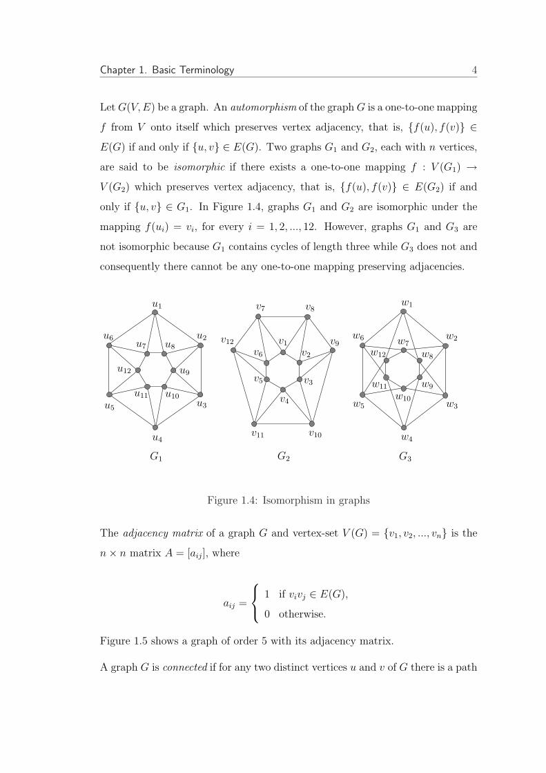
Let G(V,E) be a graph. An automorphism of the graph G is a one-to-one mapping
f from V onto itself which preserves vertex adjacency, that is, f(u), f(v) ∈E(G) if and only if u, v ∈ E(G). Two graphs G1 and G2, each with n vertices,
are said to be isomorphic if there exists a one-to-one mapping f : V (G1) →V (G2) which preserves vertex adjacency, that is, f(u), f(v) ∈ E(G2) if and
only if u, v ∈ G1. In Figure 1.4, graphs G1 and G2 are isomorphic under the
mapping f(ui) = vi, for every i = 1, 2, ..., 12. However, graphs G1 and G3 are
not isomorphic because G1 contains cycles of length three while G3 does not and
consequently there cannot be any one-to-one mapping preserving adjacencies.
w12
w5
w6
w10w3
w2
G3
v11
u2
w4
v8
v10
v1
v2v6
v5 v3
v4
v9
G2
u8
u9
u11 u10
u7
u1
u4
G1
v12
u12
u6
v7
u5
w1
u3
w9
w8
w7
w11
Figure 1.4: Isomorphism in graphs
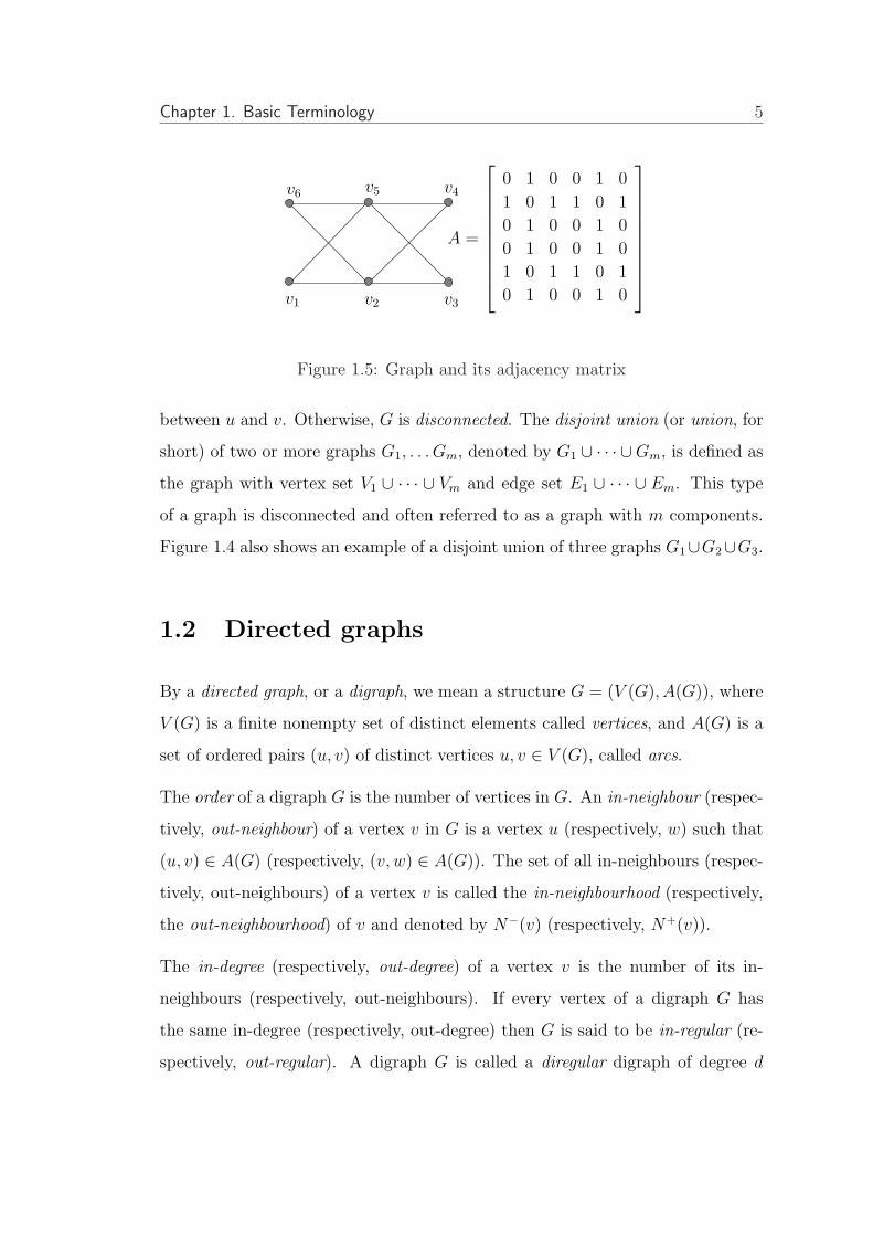
The adjacency matrix of a graph G and vertex-set V (G) = v1, v2, ..., vn is the
n× n matrix A = [aij], where
aij =
1 if vivj ∈ E(G),
0 otherwise.
Figure 1.5 shows a graph of order 5 with its adjacency matrix.
A graph G is connected if for any two distinct vertices u and v of G there is a path
Chapter 1. Basic Terminology 5
A =
0 1 0 0 1 0
1 0 1 1 0 1
0 1 0 0 1 0
0 1 0 0 1 0
1 0 1 1 0 1
0 1 0 0 1 0
v1 v2 v3
v6 v5 v4
Figure 1.5: Graph and its adjacency matrix
between u and v. Otherwise, G is disconnected. The disjoint union (or union, for
short) of two or more graphs G1, . . . Gm, denoted by G1 ∪ · · · ∪Gm, is defined as
the graph with vertex set V1 ∪ · · · ∪ Vm and edge set E1 ∪ · · · ∪ Em. This type
of a graph is disconnected and often referred to as a graph with m components.
Figure 1.4 also shows an example of a disjoint union of three graphs G1∪G2∪G3.
1.2 Directed graphs
By a directed graph, or a digraph, we mean a structure G = (V (G), A(G)), where
V (G) is a finite nonempty set of distinct elements called vertices, and A(G) is a
set of ordered pairs (u, v) of distinct vertices u, v ∈ V (G), called arcs.
The order of a digraph G is the number of vertices in G. An in-neighbour (respec-
tively, out-neighbour) of a vertex v in G is a vertex u (respectively, w) such that
(u, v) ∈ A(G) (respectively, (v, w) ∈ A(G)). The set of all in-neighbours (respec-
tively, out-neighbours) of a vertex v is called the in-neighbourhood (respectively,
the out-neighbourhood) of v and denoted by N−(v) (respectively, N+(v)).
The in-degree (respectively, out-degree) of a vertex v is the number of its in-
neighbours (respectively, out-neighbours). If every vertex of a digraph G has
the same in-degree (respectively, out-degree) then G is said to be in-regular (re-
spectively, out-regular). A digraph G is called a diregular digraph of degree d

Chapter 1. Basic Terminology 6
if G is in-regular of in-degree d and out-regular of out-degree d. For example,
the digraph G1 in Figure 1.6 is diregular of degree 2, but the digraph G2 is not
diregular (G2 is out-regular but not in-regular). The in-degree sequence (respec-
tively, out-degree sequence) of a digraph G is the sequence obtained by listing the
vertex in-degree (respectively, out-degree) of G in increasing order, with repeats
as necessary.
v2
v3
G1v4 v5
v1
G2
v2 v3
v4 v5
v1
Figure 1.6: Diregular and non-diregular digraphs.
A digraph H is a subdigraph of G if every vertex of H is a vertex of G, and every
arc of H is an arc of G. In other words, V (H) ⊂ V (G) and A(H) ⊂ A(G).
We say that a subdigraph H is a spanning subdigraph of G if H contains all the
vertices of G. Let F be a nonempty subset of the vertex set V (G). The induced
subdigraph G[F ] is a subdigraph of G consisting of the vertex-set F together with
all the arcs uv of G, where u, v ∈ F .
An alternating sequence v0a1v1a2...akvk of vertices and arcs in G such that ai =
(vi−1, vi), for each i, 1 ≤ i ≤ k, is called a walk of length k in G. A walk is closed
if v0 = vk. If all the vertices of a v0 − vk walk are distinct, then such a walk is
called a path. A cycle is a closed path. A digon is a cycle of length 2.
The distance from vertex u to vertex v, denoted by δ(u, v), is the length of a
shortest path from u to v, if any; otherwise, δ(u, v) = ∞. Note that, in general,
δ(u, v) is not necessarily equal to δ(v, u). The in-eccentricity of v, denoted by
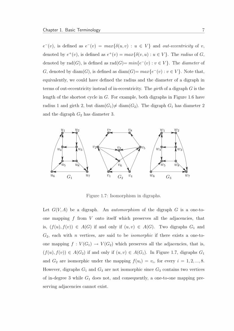
Chapter 1. Basic Terminology 7
e−(v), is defined as e−(v) = maxδ(u, v) : u ∈ V and out-eccentricity of v,
denoted by e+(v), is defined as e+(v) = maxδ(v, u) : u ∈ V . The radius of G,
denoted by rad(G), is defined as rad(G)= mine−(v) : v ∈ V . The diameter of
G, denoted by diam(G), is defined as diam(G)= maxe−(v) : v ∈ V . Note that,
equivalently, we could have defined the radius and the diameter of a digraph in
terms of out-eccentricity instead of in-eccentricity. The girth of a digraph G is the
length of the shortest cycle in G. For example, both digraphs in Figure 1.6 have
radius 1 and girth 2, but diam(G1)6= diam(G2). The digraph G1 has diameter 2
and the digraph G2 has diameter 3.
w4
u5
u6 u7G1
v2
v1 v4
v5v3
v6
G2
v7 v8
u4
w1 w2
w8w5
w6 w7G3
u3 w3
u1 u2
u8
Figure 1.7: Isomorphism in digraphs.
Let G(V,A) be a digraph. An automorphism of the digraph G is a one-to-
one mapping f from V onto itself which preserves all the adjacencies, that
is, (f(u), f(v)) ∈ A(G) if and only if (u, v) ∈ A(G). Two digraphs G1 and
G2, each with n vertices, are said to be isomorphic if there exists a one-to-
one mapping f : V (G1) → V (G2) which preserves all the adjacencies, that is,
(f(u), f(v)) ∈ A(G2) if and only if (u, v) ∈ A(G1). In Figure 1.7, digraphs G1
and G2 are isomorphic under the mapping f(ui) = vi, for every i = 1, 2, ..., 8.
However, digraphs G1 and G3 are not isomorphic since G3 contains two vertices
of in-degree 3 while G1 does not, and consequently, a one-to-one mapping pre-
serving adjacencies cannot exist.
Chapter 1. Basic Terminology 8
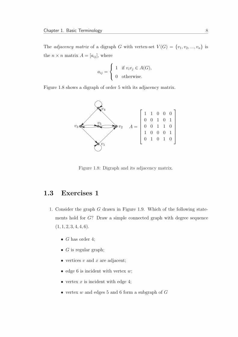
The adjacency matrix of a digraph G with vertex-set V (G) = v1, v2, ..., vn is
the n× n matrix A = [aij], where
aij =
1 if vivj ∈ A(G),
0 otherwise.
Figure 1.8 shows a digraph of order 5 with its adjacency matrix.
v2
v5
v4
v3
v1
A =
1 1 0 0 0
0 0 1 0 1
0 0 1 1 0
1 0 0 0 1
0 1 0 1 0
Figure 1.8: Digraph and its adjacency matrix.
1.3 Exercises 1
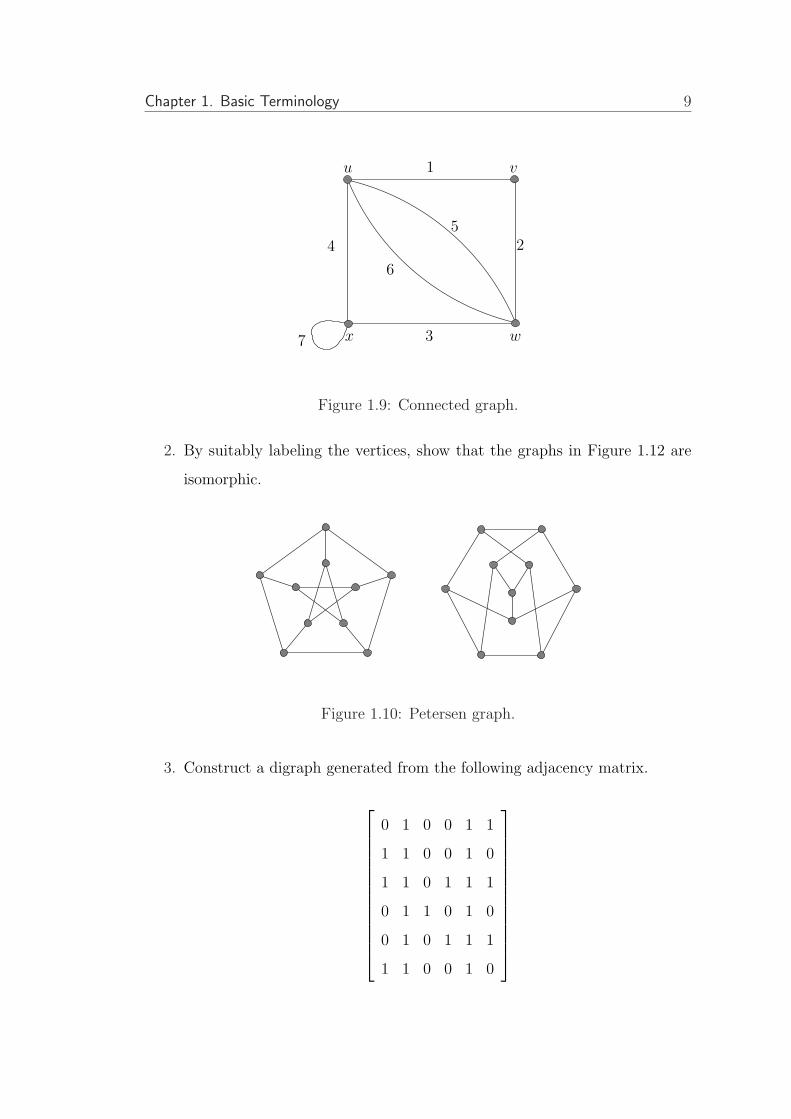
1. Consider the graph G drawn in Figure 1.9. Which of the following state-
ments hold for G? Draw a simple connected graph with degree sequence
(1, 1, 2, 3, 4, 4, 6).
• G has order 4;
• G is regular graph;
• vertices v and x are adjacent;
• edge 6 is incident with vertex w;
• vertex x is incident with edge 4;
• vertex w and edges 5 and 6 form a subgraph of G
Chapter 1. Basic Terminology 9
7
6
24
w3x
u 1 v
5
Figure 1.9: Connected graph.
2. By suitably labeling the vertices, show that the graphs in Figure 1.12 are
isomorphic.
Figure 1.10: Petersen graph.
3. Construct a digraph generated from the following adjacency matrix.
0 1 0 0 1 1
1 1 0 0 1 0
1 1 0 1 1 1
0 1 1 0 1 0
0 1 0 1 1 1
1 1 0 0 1 0

Chapter 1. Basic Terminology 10
4. By suitably labeling the vertices, show that two of the following digraphs
are isomorphic.
G3G2G1
Figure 1.11: Isomorphism in digraphs.
5. Which of the following digraphs is subdigraph of the digraph G below?
Draw one of the other spanning subdigraph of digraph G.
v2
G2
v1
v3
v5G1
v1
v3
v5
v6
G
v2 v4 v2 v4 v4
v1
v3
v5
Figure 1.12: Digraph and its subdigraph.
6. Write down the adjacency matrix of each of the digraphs presented in Figure
1.13.
7. A food web involves ten species, 1, 2, . . . , 10, with the following behaviour:
species 1 eats species 3,7,10; species 2 eats species 7; species 3 eats species
5, 7; species 4 eats species 2,5,6,8,10; species 5 eats species 6, 9; species
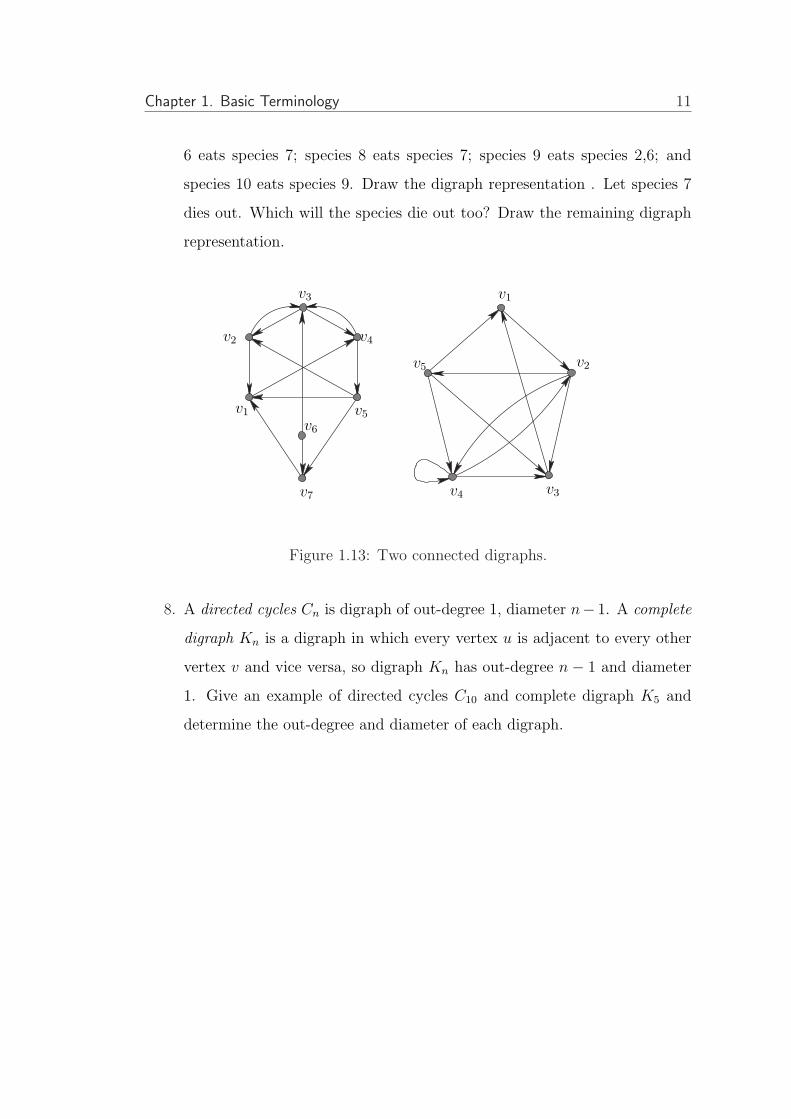
Chapter 1. Basic Terminology 11
6 eats species 7; species 8 eats species 7; species 9 eats species 2,6; and
species 10 eats species 9. Draw the digraph representation . Let species 7
dies out. Which will the species die out too? Draw the remaining digraph
representation.
v1
v7
v2 v4
v1v3
v5 v2
v6
v5
v4 v3
Figure 1.13: Two connected digraphs.
8. A directed cycles Cn is digraph of out-degree 1, diameter n− 1. A complete
digraph Kn is a digraph in which every vertex u is adjacent to every other
vertex v and vice versa, so digraph Kn has out-degree n − 1 and diameter
1. Give an example of directed cycles C10 and complete digraph K5 and
determine the out-degree and diameter of each digraph.
Modul 2
Some Applications of Graphs
2.1 Applications of Graphs
Graph Theory is one of the branch of Discrete Mathematics. This subject nor-
mally studies some discrete phenomenons. The phenomenon is said to be discrete
when it only deals with some discontinued finite elements. The integer set is
usually considered to be a discrete object. Discrete Mathematics Model grows
intensively in all aspect of modern society. One of the factors is due to the ad-
vance of information and communication technology. The data storage system in
computer is manipulated in discrete format.
Some examples fragmently categorized as Discrete Mathematics Model are Com-
putation Models, Algorithm Complexity, Graph Representation, and many oth-
ers. In this book, we focus on the study of graph modeling. The use of graph
in many field is to model a real phenomenon, for examples chemical compound
representation, computer database, programming debugging, Konigsberg bridge
problem, utilities problem, road network and communication network.
Chemical Compound
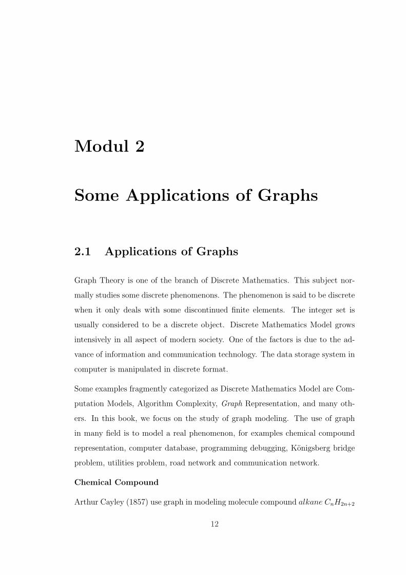
Arthur Cayley (1857) use graph in modeling molecule compound alkane CnH2n+2
12
Chapter 2. Some Applications of Graphs 13
to count the number of their isomer. Carbon atom C and hydrogen atom H are
considered to be a vertex or node, and the links between atom C and H are
considereded to be an edge.
Etana (C2H6) Propana (C3H8)
H H
H
H
C
Metana (CH4)
Figure 2.1: Alkane compound: Metane, Etane and Propane.
Konigsberg Bridge Problem
The very first problem in graph modeling was the Konigsberg bridge problem. In
Konigsberg there are seven bridges over the delta area of the Pregel river. The
Pregel divides Konigsberg into two islands and two banks, see Figure 2.2. The
problem was to begin at any bridge, cross all seven bridges excatly once, and
return to the starting point.
No one ever succeded in doing this, and Leonhard Euler gave a proof that this
was impossible. In 1736 he wrote the first graph paper about the Konigsberg
bridge problem. This problem is now known as Eulerian and Hamiltonian cycle
problems.

Chapter 2. Some Applications of Graphs 14
Figure 2.2: Konigsberg city.
Figure 2.3: The Konigsberg bridge.
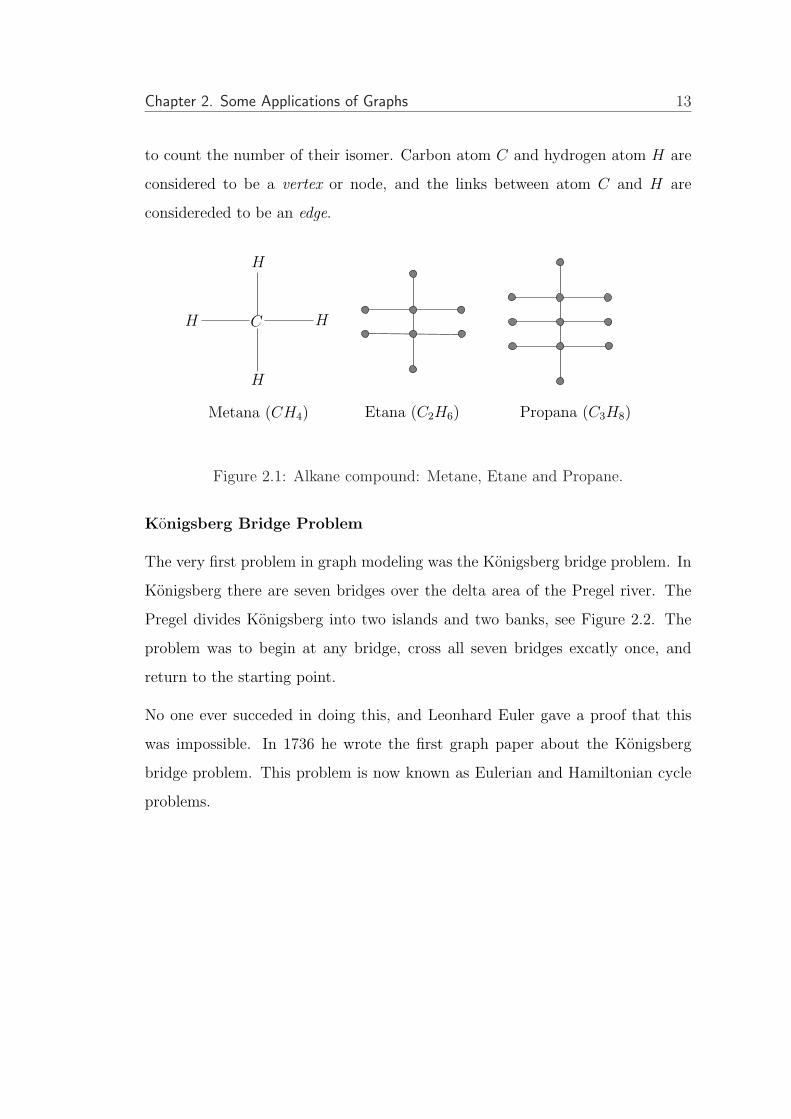
Road Network
In a road network, the weight of each arc (road) may correspond to any of the
following: its length in miles or kilometers; the estimated or actual time taken
to travel along it; the cost involved in traveling along it (fuel, fare, etc.). For
example, the map in Figure 2.2, shows some of the major routes between a
number of cities in USA, where the numbers indicate the driving times (in hours)
between pairs of cities. We wish to find the shortest time taken to drive from Los
Angeles to Amarillo, and from San Francisco to Denver. This problem is related
to the well-known problem called Shortest Path problem.
Chapter 2. Some Applications of Graphs 15
Figure 2.4: A road map of cities in USA.
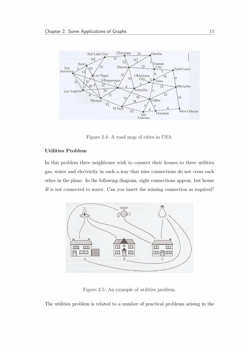
Utilities Problem
In this problem three neighbours wish to connect their houses to three utilities
gas, water and electricity in such a way that nine connections do not cross each
other in the plane. In the following diagram, eight connections appear, but house
B is not connected to water. Can you insert the missing connection as required?
Figure 2.5: An example of utilities problem.
The utilities problem is related to a number of practical problems arising in the

Chapter 2. Some Applications of Graphs 16
Figure 2.6: Portion of a printed circuit.
study of printed circuits design for use in electronics devices. In this problems,
electronic components are constructed by means of conducting strips printed di-
rectly on a flat board of insulating material. Such printed connectors can not
cross one another, since this would lead to undesirable electrical contact at cross-
ing points. This problem leads to the well-known problem called planarity of
graph.
Communication Network
There are basically two types of networks, static networks and dynamic networks.
The static type of network is a network that is established and grows according to
a topological design developed by some central authority or administration. The
topology of such a network is fixed and well defined. Many well-known structures,
such as ring, bus, hierarchical, tree, star, hyper cube, etc, have been engaged in
this type of networks, see Figure 2.7. A public telephone switch system is an
example of static network and in general it follows the star structure. Large
networks often contain segments of star, ring, hierarchical and bus topologies, see
Figure 2.8.

Chapter 2. Some Applications of Graphs 17
Figure 2.7: Network topologies.
Figure 2.8: Combination of network topologies.
Chapter 2. Some Applications of Graphs 18
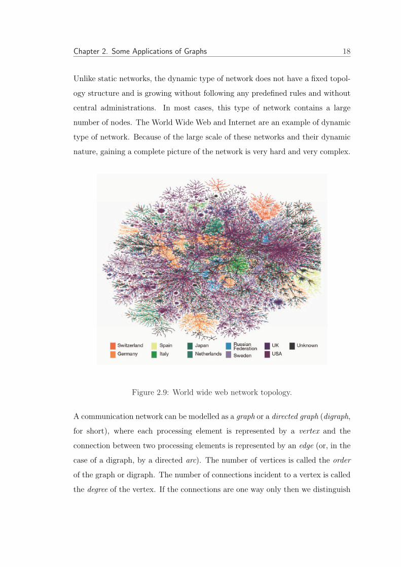
Unlike static networks, the dynamic type of network does not have a fixed topol-
ogy structure and is growing without following any predefined rules and without
central administrations. In most cases, this type of network contains a large
number of nodes. The World Wide Web and Internet are an example of dynamic
type of network. Because of the large scale of these networks and their dynamic
nature, gaining a complete picture of the network is very hard and very complex.
Figure 2.9: World wide web network topology.
A communication network can be modelled as a graph or a directed graph (digraph,
for short), where each processing element is represented by a vertex and the
connection between two processing elements is represented by an edge (or, in the
case of a digraph, by a directed arc). The number of vertices is called the order
of the graph or digraph. The number of connections incident to a vertex is called
the degree of the vertex. If the connections are one way only then we distinguish
Chapter 2. Some Applications of Graphs 19
between in-coming and out-going connections and we speak of the in-degree and
the out-degree of a vertex. The distance between two vertices is the length of the
shortest path, measured by the number of edges or arcs that need to be traversed
in order to reach one vertex from another vertex. In either case, the largest
distance between any two vertices, called the diameter of the graph or digraph,
represents the maximum data communication delay in a communication network.
For undirected case of networks, translating the above required conditions in
terms of the underlying digraphs, the problem is to find large graphs with given
maximum degree and diameter. This naturally leads to the well-known funda-
mental problem called the degree/diameter problem: For given numbers ∆ and
D, construct graphs of maximum degree ∆ and diameter ≤ D, with the largest
possible number of vertices n∆,D. The directed version of the problem differs only
in that ‘degree’ is replaced by ‘out-degree’ in the statement of the problem.
2.2 Classifying Problems
It is useful to consider a classification of problems based on four types of question
that commonly arise. They are as follows.
1. Existence problem. Does there exist . . . ? Is it possible to . . . ?
2. Construction problem. If . . . exist, how can we construct it?
3. Enumeration problem. How many . . . are there? Can we list them all?
4. Optimization problem. If there are several . . . , which one is the best?

Chapter 2. Some Applications of Graphs 20
2.3 Exercises 2
1. Show that there is just one alkane with formula C3H8, but there are two
alkanes with formula C4H10. Consider the alkanes CnH2n+2 for n = 5, and
construct all the possible molecules.
2. Consider the transaction system depicted in Figure 2.13(G3). Delete some
arcs if necessary in such a way the transaction system will not be deadlock.
3. Find an example of listing programming of any programming language and
construct its directed graph flow.
Figure 2.10: Map of Jember.
4. Construct a graph, apart from cycle, with the biggest possible number of
order in such a way you can find a route crossing each edge just once and
returning to the starting vertex.

Chapter 2. Some Applications of Graphs 21
v6
v8
v1 v2
v5 v4
v3v6
v6 v5 v4 v3
v1 v2
G1 G2 G3
v9
v1
v2
v3
v4
v5
v7
Figure 2.11: Some examples of planar graph.
5. Consider Jember region map depicted in Figure 2.10. Draw its graph repre-
sentation and label a number on each edge to represent an estimated time
taken to travel along two regions. Find the shortest time taken to travel
from Sumberbaru to Tempurejo.
G2G1
Figure 2.12: Two examples of undirected graph.
6. Show that the graphs in Figure 2.11 are planar. (Hint : A graph G is planar
if it can be drawn in the plane in such a way that no two edges meet except
at a vertex with which they are both incident).
7. Tabulate all information respected to order, degree, in/out-degree and di-
Chapter 2. Some Applications of Graphs 22
ameter of the digraphs showed in Figure 2.12 and Figure 2.13.
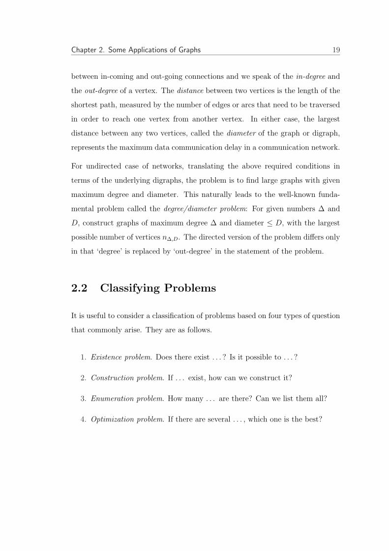
8. For given out-degree ∆ = 3 and diameter D = 2, construct a directed
graph with the biggest possible number of vertices n∆,D. For given out-
degree d = 2 and diameter k = 2, construct a directed graph with the
biggest possible number of vertices nd,k.
G2G1
G3
Figure 2.13: Three examples of directed graph.
Modul 3
Planarity of Graph
3.1 Planar Graph
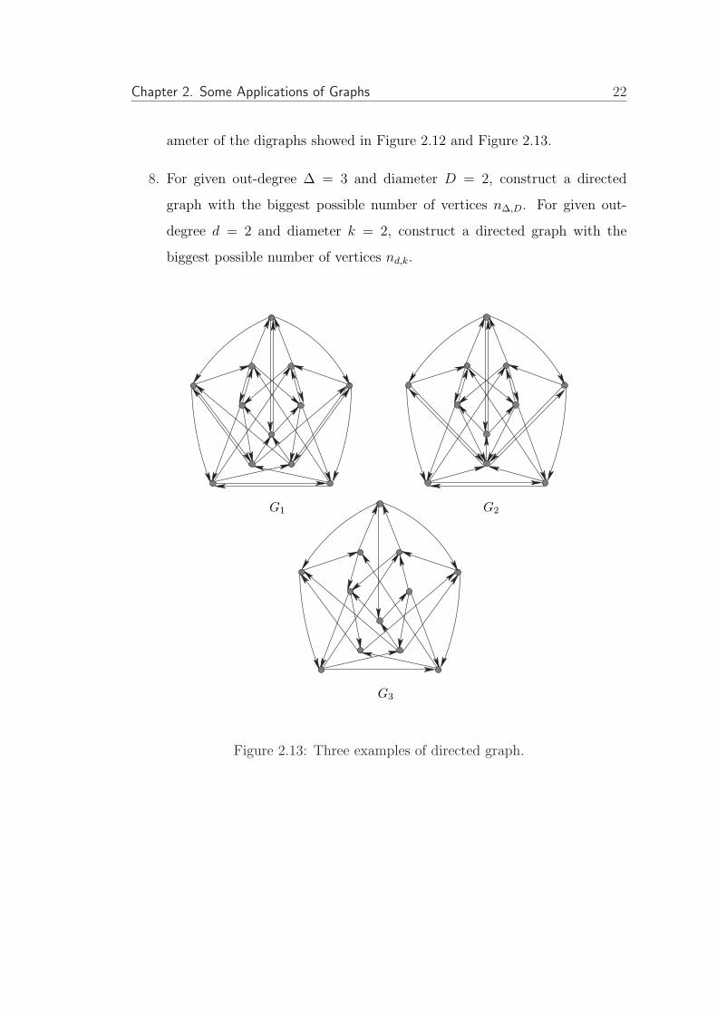
Definition 3.1.1 A graph G is planar if it can be drawn in the plan in such
away that no two edges meet except at a vertex with which they are both incident.
Any such drawing is a plane drawing of G. A graph G is non-planar if no plane
drawing of G exist.
A plan drawing of K4K4
Figure 3.1: The graph with its planar graph
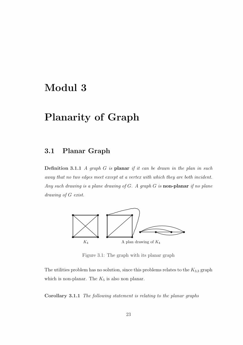
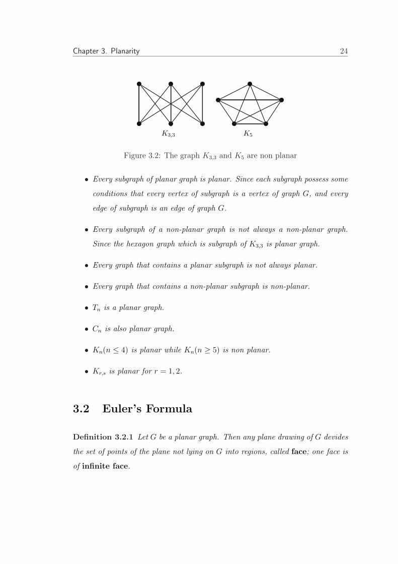
The utilities problem has no solution, since this problems relates to the K3,3 graph
which is non-planar. The K5 is also non planar.
Corollary 3.1.1 The following statement is relating to the planar graphs
23
Chapter 3. Planarity 24
K5K3,3
Figure 3.2: The graph K3,3 and K5 are non planar
• Every subgraph of planar graph is planar. Since each subgraph possess some
conditions that every vertex of subgraph is a vertex of graph G, and every
edge of subgraph is an edge of graph G.
• Every subgraph of a non-planar graph is not always a non-planar graph.
Since the hexagon graph which is subgraph of K3,3 is planar graph.
• Every graph that contains a planar subgraph is not always planar.
• Every graph that contains a non-planar subgraph is non-planar.
• Tn is a planar graph.
• Cn is also planar graph.
• Kn(n ≤ 4) is planar while Kn(n ≥ 5) is non planar.
• Kr,s is planar for r = 1, 2.
3.2 Euler’s Formula
Definition 3.2.1 Let G be a planar graph. Then any plane drawing of G devides
the set of points of the plane not lying on G into regions, called face; one face is
of infinite face.
Chapter 3. Planarity 25
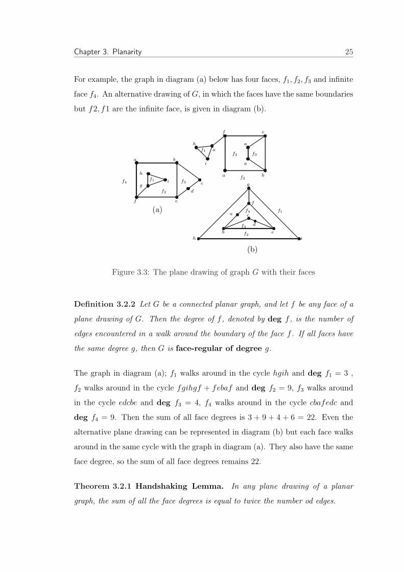
For example, the graph in diagram (a) below has four faces, f1, f2, f3 and infinite
face f4. An alternative drawing of G, in which the faces have the same boundaries
but f2, f1 are the infinite face, is given in diagram (b).
(b)
d
e
f2
f3f4
a b
c
f
f1 ig
h
a
a
a
a
b
ef
h
i
f1f4 f3
f2
a
i
f1
f2
g
f
f4c
d
b
h
e
f3
(a)
Figure 3.3: The plane drawing of graph G with their faces
Definition 3.2.2 Let G be a connected planar graph, and let f be any face of a
plane drawing of G. Then the degree of f , denoted by deg f , is the number of
edges encountered in a walk around the boundary of the face f . If all faces have
the same degree g, then G is face-regular of degree g.
The graph in diagram (a); f1 walks around in the cycle hgih and deg f1 = 3 ,
f2 walks around in the cycle fgihgf + febaf and deg f2 = 9, f3 walks around
in the cycle edcbe and deg f3 = 4, f4 walks around in the cycle cbafedc and
deg f4 = 9. Then the sum of all face degrees is 3 + 9 + 4 + 6 = 22. Even the
alternative plane drawing can be represented in diagram (b) but each face walks
around in the same cycle with the graph in diagram (a). They also have the same
face degree, so the sum of all face degrees remains 22.
Theorem 3.2.1 Handshaking Lemma. In any plane drawing of a planar
graph, the sum of all the face degrees is equal to twice the number od edges.

Chapter 3. Planarity 26
f5
u v
w
x
y
z f1
f2
f3 f4
f6
Figure 3.4: The plane drawing of planar graph
The deg f1 = 3 , deg f2 = 3, deg f3 = 2, deg f4 = 4, deg f5 = 1 and deg f6 = 7.
Then the sum of all face degrees is∑
deg f = 3 + 3 + 2 + 4 + 1 + 7 = 20 = 2.e,
where e is the number of edges.
Theorem 3.2.2 Euler’s Formula. Let G be a connected planar graph, and let
n,m and f denote, respectively, the numbers of vertices, edges and faces in a
plane drawing of G. Then
n−m + f = 2.
See proof at p. 251-252.
Corollary 3.2.1 Let G be a simple connected planar graph with n(≥ 3) vertices
and m edges. Then
m ≤ 3n− 6.
Proof. Consider a plane drawing of a simple connected planar graph G with f
faces. Since a simple graph has no loops or multiple edges, the degree of each
face is at least k. It follows from the handshaking lemma
kf ≤ 2m.
So for k=3 we have
3f ≤ 2m.
Chapter 3. Planarity 27
Substituting for f from Euler’s formula f = m− n + 2 we obtain
3m− 3n + 6 ≤ 2m,
and hence
m ≤ 3n− 6 ¥
Corollary 3.2.2 Let G be a simple connected planar graph with n(≥ 3) vertices,
m edges and no triangles. Then
m ≤ 2n− 4.
Proof. Consider a plane drawing of a simple connected planar graph G with f
faces and no triangles. The degree of each face of such a graph is at least 4. It
follows from the handshaking lemma
4f ≤ 2m.
Substituting for f from Euler’s formula f = m− n + 2 we obtain
2m− 2n + 4 ≤ m,
and hence
m ≤ 2n− 4 ¥
Corollary 3.2.3 Let G be a simple connected planar graph with n(≥ 3) vertices,
m edges and having a face-regular of degree 3 and 4. Then it gives respectively
the equalities as follow
m = 3n− 6 and m = 2n− 4.
Corollary 3.2.4 Let G be a simple connected planar graph with n(≥ 5) vertices,
m edges and shortest cycle length 5. Then
m ≤ 5
3(n− 2).
Chapter 3. Planarity 28
Proof. Consider a plane drawing of a simple connected planar graph G with f
faces. The shortest cycle length of such graph is 5. It follows from the handshak-
ing lemma
5f ≤ 2m.
Substituting for f from Euler’s formula f = m− n + 2 we obtain
5m− 5n + 10 ≤ 2m,
and hence
m ≤ 5
3(n− 2) ¥
3.3 Cycle Method for Planarity Testing
Let G be any graph. We wish to test for planarity, we look for a Hamiltonian
cycle, draw this cycle as a regular polygon, and then try to draw the remaining
edges so that no edges cross. Having chosen a Hamiltonian cycle C, we list the
remaining edges of G, and try to devide them into two disjoint sets A and B,
where A is a set of edges that can be drawn inside C without crossing and B is a
set of edges that can be drawn outside C without crossing. If this is possible, the
graph G is planar, and we can use the sets A and B to obtain a plane drawing
of G.
3.4 Kuratowski’s Theorem
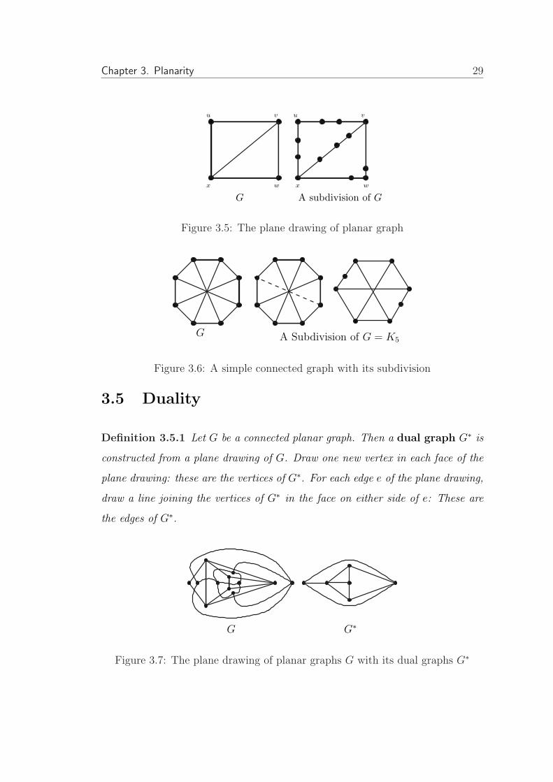
Let G be any graph, the insertion of vertices of degree 2 into the edges of G will
get a new graph namely a subdivision of G, as shown in the following diagram.
Theorem 3.4.1 A graph is planar if and only if it contains no subdivision of K5
or K3,3 and no subgraph that has K5 or K3,3 as a contraction.
Chapter 3. Planarity 29
G
u v
wx
u v
wx
A subdivision of G
Figure 3.5: The plane drawing of planar graph
A Subdivision of G = K5G
Figure 3.6: A simple connected graph with its subdivision
3.5 Duality
Definition 3.5.1 Let G be a connected planar graph. Then a dual graph G∗ is
constructed from a plane drawing of G. Draw one new vertex in each face of the
plane drawing: these are the vertices of G∗. For each edge e of the plane drawing,
draw a line joining the vertices of G∗ in the face on either side of e: These are
the edges of G∗.
G∗G
Figure 3.7: The plane drawing of planar graphs G with its dual graphs G∗
Chapter 3. Planarity 30
Proof. Let G be a plane drawing of a connected planar graph with n vertices,
m edges and f faces. Then G∗ has f vertices, m edges and f faces and the dual
of G∗ is G.
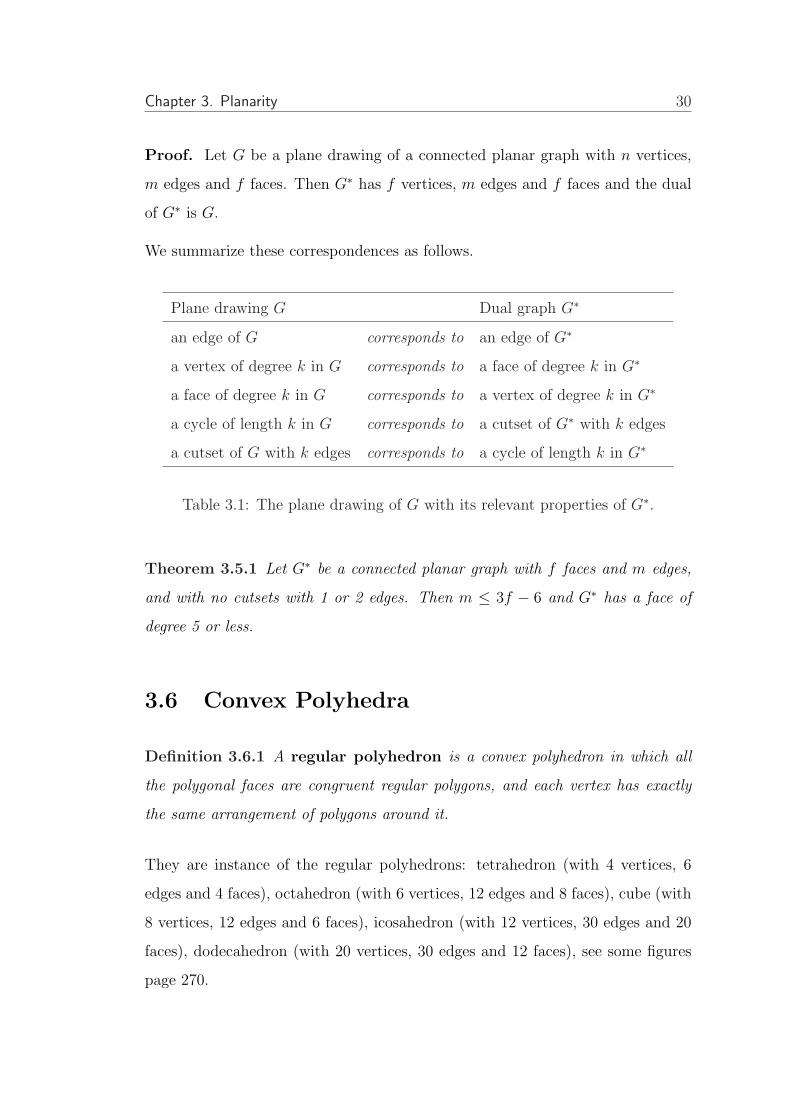
We summarize these correspondences as follows.
Plane drawing G Dual graph G∗
an edge of G corresponds to an edge of G∗
a vertex of degree k in G corresponds to a face of degree k in G∗
a face of degree k in G corresponds to a vertex of degree k in G∗
a cycle of length k in G corresponds to a cutset of G∗ with k edges
a cutset of G with k edges corresponds to a cycle of length k in G∗
Table 3.1: The plane drawing of G with its relevant properties of G∗.
Theorem 3.5.1 Let G∗ be a connected planar graph with f faces and m edges,
and with no cutsets with 1 or 2 edges. Then m ≤ 3f − 6 and G∗ has a face of
degree 5 or less.
3.6 Convex Polyhedra
Definition 3.6.1 A regular polyhedron is a convex polyhedron in which all
the polygonal faces are congruent regular polygons, and each vertex has exactly
the same arrangement of polygons around it.
They are instance of the regular polyhedrons: tetrahedron (with 4 vertices, 6
edges and 4 faces), octahedron (with 6 vertices, 12 edges and 8 faces), cube (with
8 vertices, 12 edges and 6 faces), icosahedron (with 12 vertices, 30 edges and 20
faces), dodecahedron (with 20 vertices, 30 edges and 12 faces), see some figures
page 270.
Chapter 3. Planarity 31
Theorem 3.6.1 Euler’s Polyhedron Formula. Let v, e and f denote, respec-
tively, the numbers of vertices, edges and faces of a convex polyhedron. Then
v − e + f = 2.
Theorem 3.6.2 There are only five regular polyhedra:
• three with triangular faces-the octahedron and the icosahedron;
• one with square faces-the cube;
• one with pentagonal faces-the dodecahedron.
Proof. Let v, e and f denote, respectively, the numbers of vertices, edges and
faces of a regular polyhedron with triangular faces. It follows from the handshak-
ing’s lemma that 3f = 2e. If exactly d meet at each vertex, then dv = 2e. These
two results can be written as f = 23
and v = 2de. Substituting these two results
into Euler’s Polyhedron Formula, we obtain 2de− e + 2
3e = 2 or 1
d− 1
6= 1
e. Since
1e
> 0, it follows that 1d
> 16⇒ d < 6. This means that the only possible values
of d are 3,4 and 5. ¥
3.7 Exercises 3
1. Find some others application of planarity graph.
2. Give some description of what you have got.
Modul 4
Construction Techniques
In general, the techniques of constructing large digraphs can be classified into
three classes.
• Algebraic specification. By algebraic specification we mean that a di-
graph is obtained by using a construction technique specified by some alge-
braic formula. Construction techniques that can be classified as algebraic
specifications include generalised de Bruijn digraphs and generalised Kautz
digraphs.
• Expansion method. By expansion method we mean that a new digraph is
obtained from another digraph of smaller order according to some specified
rules. In this way, we start from a base digraph, then follow the procedure
to obtain a new digraph with order larger than that of the original digraph.
The construction techniques that can be classified as expansion methods
are line digraphs and partial line digraphs, de Bruijn and Kautz digraphs on
alphabets and voltage assignments.
• Reduction method. Using a reduction method, we start from a digraph
then follow some procedure to obtain a new digraph with order smaller
than that of the original digraph. The construction techniques that can
32

Chapter 4. Repeat and Construction Techniques 33
be classified as reduction methods are digon reduction and vertex deletion
scheme.
4.1 Generalised de Bruijn and Kautz Digraphs
Imase and Itoh [?] constructed digraphs for given arbitrary order n and out-degree
d, 1 < d < n, by the following procedure. Let the vertices of digraphs be labeled
by 0, 1, ..., n− 1. A vertex u is adjacent to v, if
v ≡ du + i (mod n), i = 0, 1, ..., d− 1.
For example, Figure 4.1 shows the digraph of order n = 9, out-degree d = 3 and
diameter k = 2, obtained from this construction. Note that when n = dk, the
digraphs obtained from this construction are isomorphic to the de Bruijn digraphs
of degree d and diameter k.
Miller [?] gave a construction technique which is generalised Kautz digraph for
given arbitrary order n and out-degree d, for 1 < d < n. The technique is using
the following procedure. Let the vertices of digraphs be labeled by 0, 1, ..., n− 1.
A vertex u is adjacent to v, if
v ≡ −du + i (mod n), i = 0, 1, ..., d− 1.
The digraph in Figure 4.2 is obtained from the construction for n = 9 and d = 2.
Note that when n = dk + dk−1, the digraphs obtained from this construction are
isomorphic to the Kautz digraphs of degree d and diameter k.

Chapter 4. Repeat and Construction Techniques 34
3
5
0
8
7
4
62
1
Figure 4.1: Generalised de Bruijn digraphs G ∈ G(9, 3, 2).
G8 3
40
6
1
2
5
7
Figure 4.2: Generalised Kautz digraphs G ∈ G(9, 2, 3).
4.2 Line Digraphs and Partial Line Digraphs
Let G = (V,A) and let N be the multiset of all walks of length two in G. The
line digraph of a digraph G, L(G) = (A, N), that is, the set of vertices of L(G)
is equal to the set of arcs of G and the set of arcs of L(G) is equal to the set of
walks of length two in G. This means that a vertex uv of L(G) is adjacent to a
vertex wx if and only if v = w.
The order of the line digraph L(G) is equal to the number of arcs in the digraph G.
Chapter 4. Repeat and Construction Techniques 35
L2(G)
210
1
02
01
02
21
12
10
20
G L(G)
201120
012
102
121
021
101
212 010
202 020
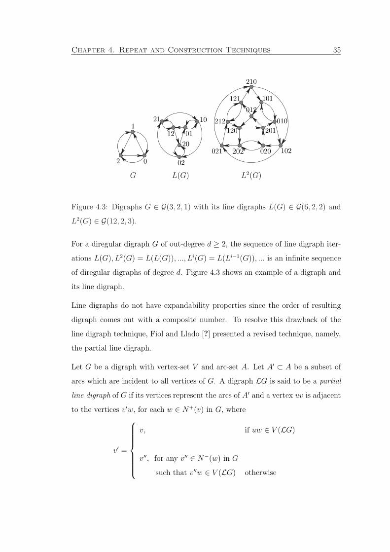
Figure 4.3: Digraphs G ∈ G(3, 2, 1) with its line digraphs L(G) ∈ G(6, 2, 2) and
L2(G) ∈ G(12, 2, 3).
For a diregular digraph G of out-degree d ≥ 2, the sequence of line digraph iter-
ations L(G), L2(G) = L(L(G)), ..., Li(G) = L(Li−1(G)), ... is an infinite sequence
of diregular digraphs of degree d. Figure 4.3 shows an example of a digraph and
its line digraph.
Line digraphs do not have expandability properties since the order of resulting
digraph comes out with a composite number. To resolve this drawback of the
line digraph technique, Fiol and Llado [?] presented a revised technique, namely,
the partial line digraph.
Let G be a digraph with vertex-set V and arc-set A. Let A′ ⊂ A be a subset of
arcs which are incident to all vertices of G. A digraph LG is said to be a partial
line digraph of G if its vertices represent the arcs of A′ and a vertex uv is adjacent
to the vertices v′w, for each w ∈ N+(v) in G, where
v′ =
v, if uw ∈ V (LG)
v′′, for any v′′ ∈ N−(w) in G
such that v′′w ∈ V (LG) otherwise
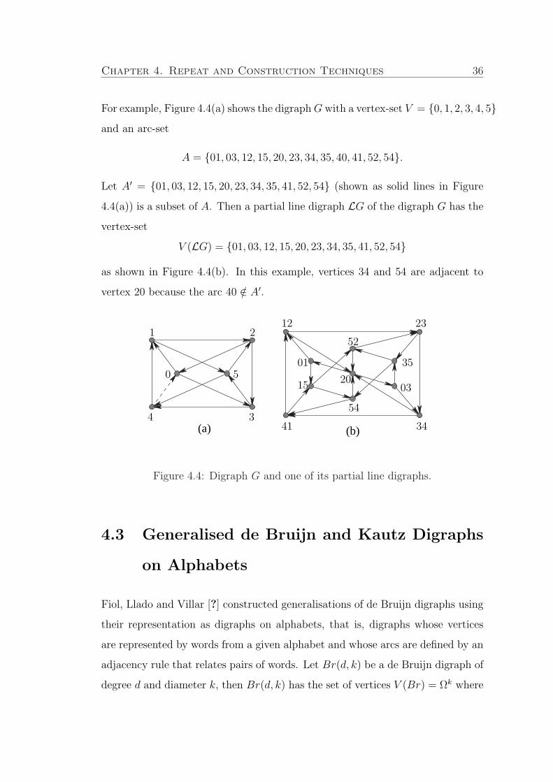
Chapter 4. Repeat and Construction Techniques 36
For example, Figure 4.4(a) shows the digraph G with a vertex-set V = 0, 1, 2, 3, 4, 5and an arc-set
A = 01, 03, 12, 15, 20, 23, 34, 35, 40, 41, 52, 54.
Let A′ = 01, 03, 12, 15, 20, 23, 34, 35, 41, 52, 54 (shown as solid lines in Figure
4.4(a)) is a subset of A. Then a partial line digraph LG of the digraph G has the
vertex-set
V (LG) = 01, 03, 12, 15, 20, 23, 34, 35, 41, 52, 54
as shown in Figure 4.4(b). In this example, vertices 34 and 54 are adjacent to
vertex 20 because the arc 40 /∈ A′.
(a) (b)
15
1 2
34
50
12 23
3441
52
54
01
2003
35
Figure 4.4: Digraph G and one of its partial line digraphs.
4.3 Generalised de Bruijn and Kautz Digraphs
on Alphabets
Fiol, Llado and Villar [?] constructed generalisations of de Bruijn digraphs using
their representation as digraphs on alphabets, that is, digraphs whose vertices
are represented by words from a given alphabet and whose arcs are defined by an
adjacency rule that relates pairs of words. Let Br(d, k) be a de Bruijn digraph of
degree d and diameter k, then Br(d, k) has the set of vertices V (Br) = Ωk where
Chapter 4. Repeat and Construction Techniques 37
Ω = x|x ∈ words and |Ω| = d and the adjacency: a vertex x1x2 . . . xk adjacent
to the vertices x2 . . . xkxk+1 for xk+1 ∈ Ω.
The generalisation of Kautz digraphs was defined as follows. Consider the vertex-
set V (Ka(d, k)) of Kautz sequences or words of length k without consecutive
letters on an alphabet X, |X| = d + 1. Let u = x1x2...xk ∈ V (Ka(d, k)) and
u be a Kautz sequence obtained from u by deleting the first letter of u, that is,
u = x2x3...xk ∈ V (Ka(d, k − 1)). Let n be any integer such that dk−1 + dk−2 <
n ≤ dk + dk−1. A digraph H(d, k, n) has vertex-set V ⊂ V (Ka(d, k)), such that
u|u ∈ V = V (Ka(d, k − 1)) and a vertex u = x1x2...xk is adjacent to the
vertices v = x′2x3...xkα for every α ∈ X, α 6= xk, where
x′2 =
x2, if x2x3...xkα ∈ V
x′′2, for any x′′2 such that
x′′2x3...xkα ∈ V , otherwise
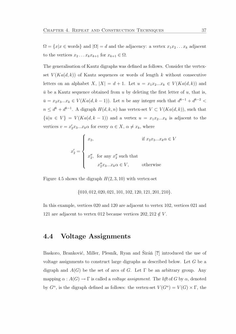
Figure 4.5 shows the digraph H(2, 3, 10) with vertex-set
010, 012, 020, 021, 101, 102, 120, 121, 201, 210.
In this example, vertices 020 and 120 are adjacent to vertex 102, vertices 021 and
121 are adjacent to vertex 012 because vertices 202, 212 /∈ V .
4.4 Voltage Assignments
Baskoro, Brankovic, Miller, Plesnık, Ryan and Siran [?] introduced the use of
voltage assignments to construct large digraphs as described below. Let G be a
digraph and A(G) be the set of arcs of G. Let Γ be an arbitrary group. Any
mapping α : A(G) → Γ is called a voltage assignment. The lift of G by α, denoted
by Gα, is the digraph defined as follows: the vertex-set V (Gα) = V (G) × Γ, the

Chapter 4. Repeat and Construction Techniques 38
121
012
021120
101
010
201
020
210
102
Figure 4.5: Example of generalised Kautz digraph on alphabet.
arc-set A(Gα) = A(G) × Γ, and there is an arc (a, f) in Gα from (u, g) to (v, h)
if and only if f = g, a is an arc from u to v, and h = gα(a).
For example, Figure 4.6 shows a digraph G and its lift Gα with Γ = Z6 and the
voltage assignment α(a) = α(d) = 5, α(b) = 0, α(c) = α(f) = 1 and α(e) = 2.
Informally, voltage assignment technique enables us to “blow up” a given base
digraph G in order to obtain a larger digraph (called a “lift”) whose incidence
structure depends on both G and a mapping (“voltage assignment”) from the
edge set of G into a finite group. Since the lift is completely determined in
terms of the original base digraph G and the voltage assignment α, this type of
construction is suitable for handling large digraphs in terms of the properties of
the base digraph and the assignment.
The main problem in this technique is how to find the proper voltage assignment
value which gives a large digraph with minimum diameter k for a given out-degree
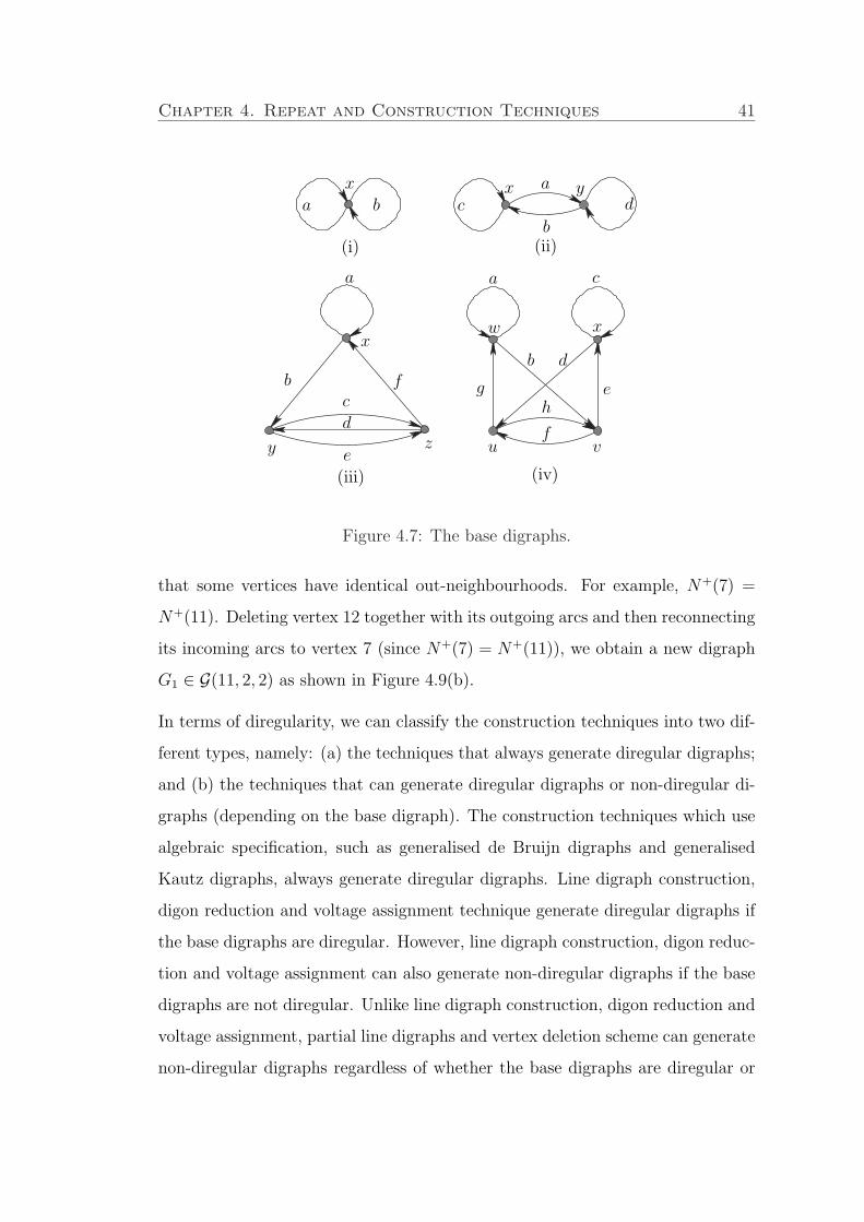
d. We developed a programming in order to find this value. By means of this
programming, we present some proper voltage assignment values in Table 4.1 by
using the base digraphs in Figure 4.7.

Chapter 4. Repeat and Construction Techniques 39
Table 4.1: The list of voltage assignment values for given k and 3 ≤ n ≤ 18, basedigraph and group Γ.
n k VA Values Base GroupDigraph
3 N/A4 2 1,2,1,3,2,1,2,3,3,1,3,2 (i) Z4
5 N/A6 2 1,0,0,2,1,0,1,2,1,0,2,2,1,1,0,2
1,1,1,2,1,1,2,2,1,2,0,2,1,2,1,21,2,2,2,2,0,0,1,2,0,1,1,2,0,2,1 (ii) Z3
2,1,0,1,2,1,1,1,2,1,2,1,2,2,0,12,2,1,1,2,2,1,1
7 N/A8 3 1,3,1,6,2,3,2,7,3,1,3,2,5,6
5,7,6,1,6,5,7,2,7,5 (i) Z8
10 3 1,0,0,4,1,0,2,2,1,0,3,2,1,0,4,3,1,1,0,31,1,1,2,1,1,3,3,1,1,4,4,1,2,0,2,1,2,1,21,2,2,3,1,2,3,4,1,2,4,3,1,3,0,2,1,3,1,31,3,2,4,1,3,3,3,1,3,4,2,1,4,0,3,1,4,1,41,4,2,3,1,4,3,2,1,4,4,2,2,0,0,3,2,1,1,42,1,2,1,2,1,3,4,2,1,4,3,2,2,0,1,2,2,1,12,2,2,4,2,2,3,3,2,2,4,4,2,3,0,1,2,3,1,42,3,2,3,2,3,3,4,2,3,4,1,2,4,1,3,2,4,2,42,4,3,1,2,4,4,1,3,0,0,2,3,0,1,1,3,0,2,4 (ii) Z5
3,0,3,4,3,0,4,1,3,1,0,1,3,1,1,4,3,1,2,43,1,3,1,3,1,4,2,3,2,0,4,3,2,1,4,3,2,2,13,2,3,2,3,2,4,1,3,3,0,4,3,3,1,1,3,3,2,23,3,3,1,3,3,4,4,3,4,0,1,3,4,1,2,3,4,2,13,4,3,4,3,4,4,4,4,0,0,1,4,0,1,2,4,0,2,34,2,2,2,4,2,3,1,4,2,4,2,4,3,0,3,4,3,1,24,3,2,1,4,3,3,2,4,3,4,3,4,4,0,2,4,4,1,1
11 N/A12 3 1, 0, 2, 0, 0, 1, 2, 1,1, 0, 2, 0, 1, 2, 0, 2
1, 0, 2, 0, 1, 2, 1, 0,1, 0, 2, 0, 1, 2, 2, 1 (iv) Z3
1, 0, 2, 1, 0, 2, 0, 2,1, 0, 2, 1, 0, 2, 1, 013 N/A16 4 3, 0, 0, 3, 1, 1, 0, 1,3, 0, 0, 3, 1, 1, 1, 0
3, 0, 0, 3, 1, 0, 3, 3,3, 0, 0, 3, 2, 0, 2, 3 (iv) Z4
1, 0, 2, 1, 0, 2, 0, 2,1, 0, 2, 1, 0, 2, 1, 018 4 5, 0, 5, 2, 1, 1,5, 0, 5, 2, 3, 5,5, 0, 5, 3, 2, 2
5, 0, 5, 4, 3, 3,5, 1, 0, 1, 2, 5,5, 1, 0, 1, 4, 3 (iii) Z6
5, 1, 0, 1, 4, 3,5, 1, 0, 3, 4, 1,5, 1, 0, 5, 2, 1

Chapter 4. Repeat and Construction Techniques 40
G
7 8
6
18
cde
b
f
a
32
1
Gα
10
12
9
1714
15 16
11 13
4 5
1 23
Figure 4.6: Digraph G and its lift Gα.
4.5 Digon Reduction and Vertex Deletion Scheme
Miller and Fris [?] gave a construction technique for digraphs of degree 2 with
minimum diameter using digon reduction scheme which they combined with line
digraph iterations. Let G ∈ G(n, d, k) be a digraph of order n, out-degree d = 2
and diameter k which contains p digons. Then G′ ∈ G(n − 1, d, k′), for k′ ≤ k,
can be obtained from G by ‘gluing’ two vertices which share a digon. Figure 4.8
shows the digraph G′ which is obtained from digraph G by gluing two vertices y
and z.
Miller and Slamin [?] also constructed digraphs using vertex deletion scheme.
Suppose that N+(u) = N+(v) for any vertex u, v ∈ G. Let G1 be a digraph
deduced from G by deleting vertex u together with its outgoing arcs and recon-
necting the incoming arcs of u to the vertex v. Obviously, the new digraph G1
has maximum out-degree the same as the maximum out-degree of G. It can be
proved that the diameter of G1 is at most k.
Figure 4.9(a) shows an example of digraph G ∈ G(12, 2, 3) with the property
Chapter 4. Repeat and Construction Techniques 41
(ii)
a b dc
a
b
yx
(i)
u v
b d
e
f
gh
y z
bc
d
e
f
x
(iv)(iii)
w x
a a c
x
Figure 4.7: The base digraphs.
that some vertices have identical out-neighbourhoods. For example, N+(7) =
N+(11). Deleting vertex 12 together with its outgoing arcs and then reconnecting
its incoming arcs to vertex 7 (since N+(7) = N+(11)), we obtain a new digraph
G1 ∈ G(11, 2, 2) as shown in Figure 4.9(b).
In terms of diregularity, we can classify the construction techniques into two dif-
ferent types, namely: (a) the techniques that always generate diregular digraphs;
and (b) the techniques that can generate diregular digraphs or non-diregular di-
graphs (depending on the base digraph). The construction techniques which use
algebraic specification, such as generalised de Bruijn digraphs and generalised
Kautz digraphs, always generate diregular digraphs. Line digraph construction,
digon reduction and voltage assignment technique generate diregular digraphs if
the base digraphs are diregular. However, line digraph construction, digon reduc-
tion and voltage assignment can also generate non-diregular digraphs if the base
digraphs are not diregular. Unlike line digraph construction, digon reduction and
voltage assignment, partial line digraphs and vertex deletion scheme can generate
non-diregular digraphs regardless of whether the base digraphs are diregular or
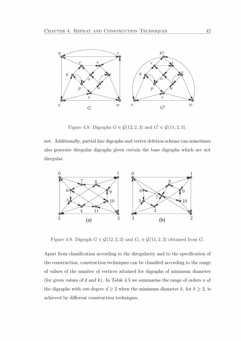
Chapter 4. Repeat and Construction Techniques 42
G′
sr
q to
up
v
x w x w
v
p u
tqo
r s
yz
G
y z
Figure 4.8: Digraphs G ∈ G(12, 2, 3) and G′ ∈ G(11, 2, 3).
not. Additionally, partial line digraphs and vertex deletion scheme can sometimes
also generate diregular digraphs given certain the base digraphs which are not
diregular.
(a) (b) 2
0 1
3
4
5
6
7 8
9
10
11
7
0 1
8
9
10
4
5
6
32
Figure 4.9: Digraph G ∈ G(12, 2, 3) and G1 ∈ G(11, 2, 3) obtained from G.
Apart from classification according to the diregularity and to the specification of
the construction, construction techniques can be classified according to the range
of values of the number of vertices attained for digraphs of minimum diameter
(for given values of d and k). In Table 4.5 we summarise the range of orders n of
the digraphs with out-degree d ≥ 2 when the minimum diameter k, for k ≥ 2, is
achieved by different construction techniques.

Chapter 4. Repeat and Construction Techniques 43
Table 4.2: Range of orders n when minimum diameter is achieved by different
techniques.
Technique Order
Generalised de Bruijn digraphs nd,k−1 < n ≤ dk
Generalised Kautz digraphs nd,k−1 < n ≤ dk or
n = dk + dk−b for odd 0 < b < k
Line digraphs nd,k−1 < n ≤ dk or
n = dk + dk−b for any 0 < b < k
Partial line digraphs nd,k−1 < n ≤ dk + dk−1 for d ≥ 3
n2,k−1 ≤ n ≤ 25× 2k−4 for k ≥ 5
Generalised Kautz digraphs nd,k−1 < n ≤ dk + dk−1
on alphabets
Digon reduction n2,k−1 < n ≤ 2k + 2k−1
Vertex deletion scheme nd,k−1 < n ≤ dk + dk−1 for d ≥ 3
n2,k−1 ≤ n ≤ 25× 2k−4 for k ≥ 4
4.6 Exercises 4
1. Write down the order and size of de Bruijn digraphs on alphabets, Kautz
digraphs on alphabets, Line digraphs, Cayley digraphs dan voltage assign-
ment digraphs. Mention some strengths and weaknesses of those construc-
tion techniques. Utilize Cayley digraphs to construct Cay(Γ5, (2, 1, 4)) dan
Cay(S3 , (13), (23)).
2. Use voltage assignment technique on a base digraph H to construct a di-
graph Hα with Γ = Z5. The voltage assignment values α are presented on
base digraph H, and also determine the diameter of the resulting digraph
Hα.
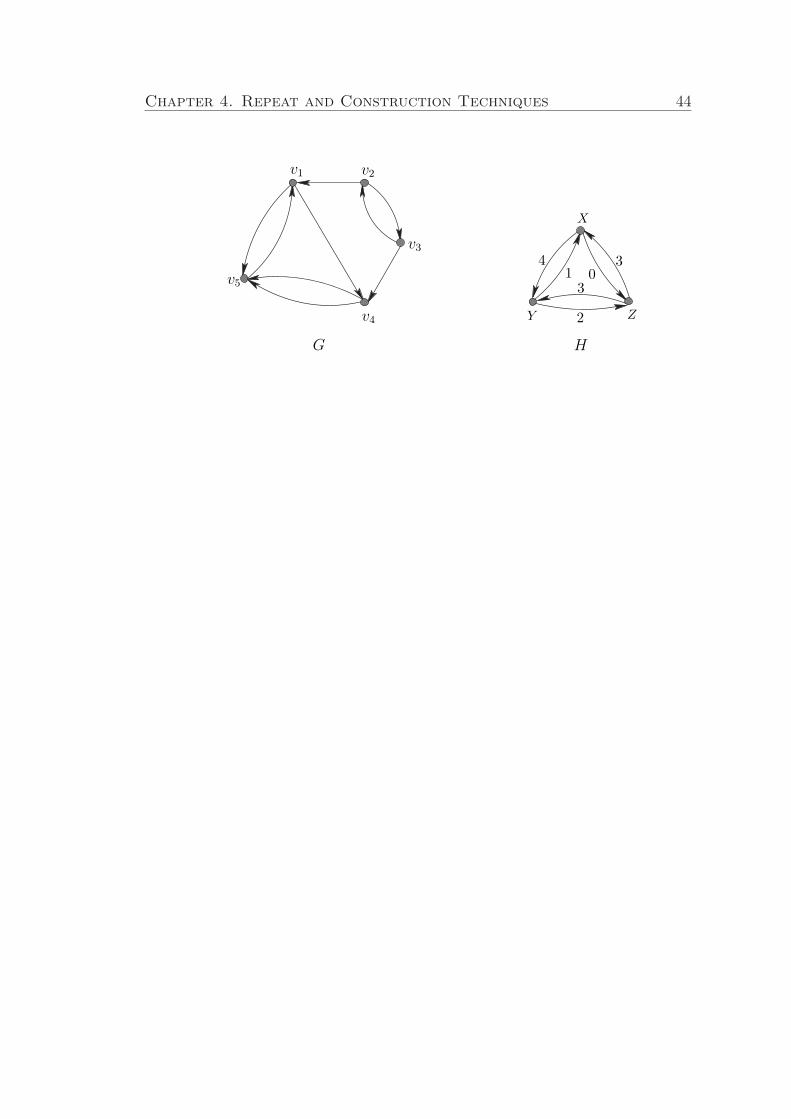
Chapter 4. Repeat and Construction Techniques 44
301
3
4
G H
2
v1 v2
v3
v5
X
ZYv4