Redalyc.ESTIMACIÓN ANALÍTICA DE LAS … · coeficiente de variación, es fundamental para una...

Agrociencia

ISSN: 1405-3195

[email protected]

Colegio de Postgraduados

México

Gómez-Gil, Jaime; Lózar-Escudero, Alfonso de; Navas-Gracia, L. Manuel; Ruiz-Ruiz, Gonzalo

ESTIMACIÓN ANALÍTICA DE LAS VARIABLES DE FUNCIONAMIENTO ÓPTIMAS DE UN

DISTRIBUIDOR CENTRÍFUGO DE FERTILIZANTE, USANDO EL MÉTODO DEL GRADIENTE

SOBRE MÚLTIPLES SEMILLAS

Agrociencia, vol. 43, núm. 5, julio-agosto, 2009, pp. 497-509

Colegio de Postgraduados

Texcoco, México

Disponible en: http://www.redalyc.org/articulo.oa?id=30211289005

Cómo citar el artículo

Número completo

Más información del artículo

Página de la revista en redalyc.org

Sistema de Información Científica

Red de Revistas Científicas de América Latina, el Caribe, España y Portugal

Proyecto académico sin fines de lucro, desarrollado bajo la iniciativa de acceso abierto

http://www.redalyc.org/revista.oa?id=302

http://www.redalyc.org/articulo.oa?id=30211289005

http://www.redalyc.org/comocitar.oa?id=30211289005

http://www.redalyc.org/fasciculo.oa?id=302&numero=11289

http://www.redalyc.org/articulo.oa?id=30211289005

http://www.redalyc.org/revista.oa?id=302

http://www.redalyc.org

497

* Autor responsable v Author for correspondence.Recibido: Agosto, 2008. Aprobado: Marzo, 2009Publicado como ARTÍCULO en Agrociencia 43: 497-509. 2009.

RESUMEN

El ajuste óptimo de las variables de funcionamiento de una

abonadora con distribuidores centrífugos para obtener un buen

coeficiente de variación, es fundamental para una distribución

uniforme del fertilizante en el terreno. En este artículo se pre-

senta una aplicación informática para predecir analíticamente el

perfil de distribución y el coeficiente de variación de abonadoras

agrícolas con distribuidores centrífugos de disco. Esta aplicación

además calcula, mediante el método del gradiente sobre múlti-

ples semillas, los valores de las variables de ajuste de la abonadora

que ofrecen un mejor coeficiente de variación. Con estos

parámetros óptimos de las variables de ajuste de la abonadora se

obtienen unos resultados de coeficiente de variación similares a

los de las marcas más prestigiosas de equipos de abonado. Se

muestra un caso particular con discos pequeños y moderada velo-

cidad de giro con el que se consigue un ancho de trabajo de 22 m,

similar a los obtenidos con equipos de abonado que tienen estos

distribuidores. El uso de esta aplicación informática en una esta-

ción de ensayo de abonadoras permite un ajuste del equipo de

abonado, reduciendo el número de ensayos experimentales re-

queridos. Esto se debe a que se realiza inicialmente una búsque-

da de los parámetros óptimos mediante la aplicación desarrolla-

da, y luego un ajuste fino de estos parámetros mediante ensayos

experimentales.

Palabras clave: Perfil de distribución, coeficiente de variación,

método del gradiente, simulador, optimizador.

INTRODUCCIÓN

E l abonado es una de las tareas más importantesque debe realizar el agricultor para aumentarel rendimiento y calidad de los cultivos. Desde

un punto de vista agronómico, económico y ambiental esmuy importante una adecuada distribución de fertilizante

ESTIMACIÓN ANALÍTICA DE LAS VARIABLES DE FUNCIONAMIENTOÓPTIMAS DE UN DISTRIBUIDOR CENTRÍFUGO DE FERTILIZANTE, USANDO

EL MÉTODO DEL GRADIENTE SOBRE MÚLTIPLES SEMILLAS

ANALYTICAL ESTIMATION OF OPTIMAL OPERATION VARIABLES OF A CENTRIFUGALFERTILIZER DISTRIBUTOR, USING THE GRADIENT METHOD ON MULTIPLE SEEDS

Jaime Gómez-Gil1*, Alfonso de-Lózar-Escudero1, L. Manuel Navas-Gracia2, Gonzalo Ruiz-Ruiz2

1Departamento de Teoría de la Señal, Comunicaciones e Ingeniería Telemática. E.T.S. Ing. deTelecomunicación. Universidad de Valladolid. ([email protected]). 2Departamento de IngenieríaAgrícola y Forestal. E.T.S. de Ingenierías Agrarias Universidad de Valladolid.

ABSTRACT

The optimal adjustment of operation variables of a fertilizer

machine with centrifugal distributors for obtaining a good

variation coefficient is essential for uniform fertilizer distribution

on farmland. This article presents a computerized application in

order to predict analytically the distribution profile and the

variation coefficient of agricultural fertilizer machines with

centrifugal disk distributors. Furthermore, this application

calculates the values of fertilizer adjustment variables, which

offer a better variation coefficient, using the gradient method on

multiple seeds. With these optimal parameters of fertilizer

adjustment variables, variation coefficient results are obtained,

similar to those of the most prestigious trademarks of fertilizing

equipment. A particular case is shown with small disks and

moderate turn speed with which a work width of 22 m is achieved,

similar to the ones obtained with the fertilizing equipment of

these distributors. The use of this computerized application in a

fertilizer machine test station allows an adjustment of the fertilizing

equipment, reducing the number of required experimental trials.

This is due to the fact that initially a search for the optimal

parameters through developed application has been carried out

and then, a fine adjustment of these parameters by means of

experimental tests.

Key words: Distribution profile, variation coefficient, gradient

method, simulator, optimizer.

INTRODUCTION

F ertilizing is one of the most important tasks thefarmer has to carry out in order to increaseyield and quality of the crop. From an

agronomical, economical, and environmental point ofview, adequate fertilizer distribution on the farmlandis very important, since a smaller dose entails nutrientshortage, and a larger one, environmental problems aswell as inadequate plant growth (Tissot et al., 2002).In both cases, the farmer will obtain lesser benefits.

498 VOLUMEN 43, NÚMERO 5

AGROCIENCIA, 1 de julio - 15 de agosto, 2009

en el terreno, ya que una dosis menor conlleva escasezde nutrientes, y una mayor, problemas ambientales asicomo un crecimiento inadecuado de la planta (Tissot etal., 2002). En ambos casos, el agricultor obtendrámenores beneficios.

Este abonado se realiza habitualmente con abonosquímicos en forma de pequeñas partículas o gránulosde fertilizante, y se esparcen con máquinas abonadoras.Los distribuidores de estas máquinas son de diferentestipos; los más habituales son los centrífugos de dosdiscos.

Un abonado homogéneo en toda la parcela requiereque el equipo presente un patrón de distribución ade-cuado durante la distribución de fertilizante. Además,el coeficiente de variación (CV) de la distancia entrepasadas a la que abona el agricultor debe ser pequeño,para una mayor uniformidad en la distribución del fer-tilizante. El estudio del patrón de distribución casi siem-pre se hace experimentalmente en estaciones de ensa-yo, principalmente por los fabricantes de los equipos.Para suplir el uso de las estaciones de ensayo, Grift yHofstee (2002) y Swisher et al. (2002) desarrollaronun método para determinar el patrón de distribuciónmediante un sensor que podía medir el diámetro y ve-locidad de las partículas que salían del disco distribui-dor.

Se han realizado estudios analíticos del comporta-miento del fertilizante en el aparato distribuidor(Olieslagers et al., 1995; Dintwa et al., 2004a; Villetteet al., 2005). Con base en dichos estudios, en el pre-sente trabajo se desarrolló una aplicación informáticaque modela el comportamiento de un distribuidor cen-trífugo, y puede buscar los parámetros del distribuidorque consigan un mejor CV. Esta búsqueda de losparámetros óptimos se realiza mediante el método delgradiente aplicado sobre múltiples semillas. Primerose presentan las ecuaciones, obtenidas de literatura cien-tífica, que modelan el comportamiento del fertilizantedentro y fuera del distribuidor centrífugo. Luego sedetalla el método para la búsqueda de los parámetrosóptimos de funcionamiento del distribuidor centrífugo.Finalmente se presentan los resultados obtenidos conla herramienta en un distribuidor centrífugo, resulta-dos acordes a los de los equipos de abonado con distri-buidores centrífugos de esas características.

MATERIALES Y MÉTODOS

La aplicación de simulación

Se usó el software de desarrollo Labview 7.1 de National

Instruments para desarrollar una aplicación informática que simula

el movimiento de las partículas de fertilizante en una abonadora

centrífuga. Este movimiento comprende desde cuando los gránulos

This fertilizing is usually carried out with chemicalfertilizers in form of small fertilizer particles or granulesbeing scattered with fertilizing machines. Thedistributors of these machines are of different types:the most usual are two-disk centrifuges.

Homogenous fertilizing all over the plot requiresthat the equipment has an appropriate distribution patternfor fertilizer distribution. Besides, the coefficient ofvariation (CV) of distance between the passes whichthe farmer fertilizes must be short in order to achievegreater uniformity in fertilizer distribution. The studyof the distribution pattern is almost always madeexperimentally at test stations, mainly by themanufacturers of the equipment. In order to supply thetest stations for use, Grift and Hofstee (2002) andSwisher et al., developed a method for determiningthe distribution pattern by means of a sensor, whichcould measure diameter and speed of the particlesleaving the distributor disk.

Analytical studies of fertilizer performance in thedistributor machine have been conducted (Olieslagerset al., 1995; Dintwa et al., 2004a; Villette et al., 2005).Based on such studies, in the present paper, acomputerized application was developed, which modelsthe performance of a centrifugal distributor and maysearch the distributor parameters achieving a better CV.This search for optimal parameters is conducted usingthe gradient method applied on multiple seeds. First,the equations obtained from scientific literature, whichmodel the fertilizer performance within and outsidethe centrifugal distributor, are presented. Then, themethod for the search of optimal operation parametersof the centrifugal distributor is detailed. Finally, theresults obtained with the tool in a centrifugal distributorare presented, results, according to those of thefertilizing equipment with centrifugal distributors ofthese characteristics.

MATERIALS AND METHODS

Simulation application

Development software Labview 7.1 of National Instruments was

used in order to develop a computerized application simulating the

movement of fertilizer particles in a centrifugal fertilizer distribution

machine. This movement covers since the moment when the granules

fall from the hopper to the distributor disk until its final position on

the soil. Starting from the position of the fertilizer on the soil, the

distribution profile and the CV obtained with the fertilizer is found.

The characteristics of the fertilizing machine (disk radius, disk turn

speed, etc.) and fertilizer granulometry must be defined by the user

of the program.

The equations on which the simulator is based are indicated

below. The calculations conducted by the program in each simulation

can be divided into three phases.

499GÓMEZ-GIL et al.

VARIABLES DE FUNCIONAMIENTO ÓPTIMAS DE UN DISTRIBUIDOR CENTRÍFUGO DE FERTILIZANTE

caen de la tolva al disco distribuidor, hasta su posición final en el

suelo. A partir de la posición del abono en el suelo se halla el perfil

de distribución y el CV obtenido con la abonadora. Las característi-

cas de la abonadora (radio de los discos, velocidad de giro de los

discos, etc.) y la granulometría del abono deben ser definidas por el

usuario del programa.

A continuación se indican las ecuaciones en que se basa el simu-

lador. Los cálculos que realiza el programa en cada simulación pue-

den dividirse en tres etapas.

Etapa 1. Movimiento de las partículas dentro del disco distribui-

dor.

Esta etapa comprende desde cuando las partículas caen de la

tolva al disco distribuidor por el orificio de alimentación, hasta que

abandonan el disco por su borde. Se supone que las aspas sobre el

disco recogen los gránulos de abono y estos gránulos, por el efecto

centrífugo, se deslizan por las aspas hasta llegar al borde del disco.

En este estudio se supone que las aspas son rectas.

El análisis matemático para calcular la trayectoria de los gránu-

los en el disco distribuidor se basa en el trabajo de Villette et al.

(2005). En esta etapa hay que obtener la velocidad absoluta de salida

de los gránulos v0, el ángulo θout de salida de las partículas, y el

ángulo recorrido Φu por las mismas mientras estaban en el disco.

La velocidad de salida v0 de los gránulos por el borde del disco

está dada por la ecuación:

v x r x sen xv lv aspa v lv v0

2 2 2= + − +&$ cos cos & &$ cos &$ cosΩ Ω Ωα θ αe j e j e j

(1)

donde, Ω es el ángulo de inclinación del disco con respecto a un

plano horizontal; αlv el ángulo de inclinación del aspa con respecto

al radio de la circunferencia que constituye el disco; θ. la velocidad

de giro de los discos (Figura 1).

La velocidad del gránulo a lo largo del aspa x. se define con la

ecuación:

&$ cos cos & exp cos &xx K

tvv

=−

+ − −0

2

b g a fa f a fd iδ

δ µ δ µ θ δ µ θΩ Ω Ω

(2)

donde, xV0 es la posición inicial de la partícula en el aspa; µ el

coeficiente de rozamiento del gránulo con el disco y el aspa; t el

tiempo que tarda el gránulo en salir del disco.

La constante K y el coeficiente δ están dados por:

Kg gsen r

sen

p=

+ −

−

µ µ θ

θ µ

cos &

& cos cos

Ω Ω

Ω Ω Ω

2

2 a f (3)

δ µ µ= + −cos cos2 2 1Ω Ω Ωd i sen (4)

Figura 1. Vista superior del disco giratorio y componentes de lavelocidad de salida de la partícula: vH=componentehorizontal de la velocidad de salida; vT=componentehorizontal tangencial de la velocidad de salida;vR=componente horizontal radial de la velocidad desalida; O, punto de giro del disco; OV, proyección de Osobre el eje del aspa; αααααlv, angulo del aspa; raspa radiodel aspa; θθθθθout ángulo entre el vector velocidad y el vectorradio en el extremo del disco; θθθθθ

. velocidad angular del

disco; rp radio del círculo tangente a las aspas.Figure 1. View from above of disk and speed components of

particle: vH=horizontal component of exit speed;vT=tangential horizontal component of exit speed;vg=radial horizontal component of exit speed; O, diskturning point; Ov, projection of O on vane axis; αααααtv,vane angle; raspa vane radius; θθθθθout angle between speedvector and radius vector at disk rim; θθθθθ

. disk angular

speed; rp tangent circle radius to vanes.

Aspa

lvanecosΩ

Ov

Vt VH

VRαlv

θout

θ

rpraspa

O

.

Phase 1. Particle movement within the distributor disk.

This phase covers from the moment when the particles fall from

the hopper through the supply opening on the distributor disk until

leaving the disk by its rim. It is assumed that the vanes on the disk

gather the fertilizer granules, and these glide, by the centrifugal

effect, along the vanes until reaching the disk rim. In this study, the

vanes are supposed to be straight.

The mathematical analysis for calculating granule trajectory on

the distributor disk is based on the study by Villette et al. (2005). In

this phase, the absolute granule exit speed v0 has to be obtained, the

particle exit angle θout, and the angle Φu covered while they were on

the disk.

Granule exit speed v0 by the disk rim is given by equation:

v x r x sen xv lv aspa v lv v0

2 2 2= + − +&$ cos cos & &$ cos &$ cosΩ Ω Ωα θ αe j e j e j

(1)

where, Ω is the angle of disk inclination with respect to a horizontal

plane; αlv the vane inclination angle with respect to the circumference

radius constituting the disk, θ. disk turn speed (Figure 1).



Para calcular el tiempo t que tarda la partícula en abandonar el

disco centrífugo se usa la ecuación (5) que presenta la posición de la

partícula respecto del aspa:

$ cos exp cos &xx K

t Kvv

=−

+ −0

2

b g a f a fd ie jδ

δ µ δ µ θΩ Ω (5)

Sustituyendo x v por lvane en (5), se obtiene el tiempo que perma-

nece el gránulo en el disco. Las ecuaciones (2) y (5) se pueden

combinar para obtener:

&$ $ cos &x x Kv v= − +b ga fδ µ θΩ (6)

La relación entre el radio de la posición del gránulo en el disco

r, y la posición de la partícula respecto del aspa x v están dadas por

la ecuación:

$

cosx

r r

rv

p= −

FHGIKJΩ

12

(7)

El ángulo de salida de la partícula θout se calcula con la ecua-

ción:

θδ µ

δ µout

aspa aspa p

aspa aspa

r l K r

l K l=

− − −

− −

F

HGG

I

KJJarctan

cos cos

cos cos

2

2

c ha fc ha f

Ω Ω

Ω Ω(8)

Finalmente, Φu, el ángulo recorrido por el disco desde que el

aspa recoge a la partícula hasta que ésta sale del disco, se halla con

la ecuación:

Φu = θ.t (9)

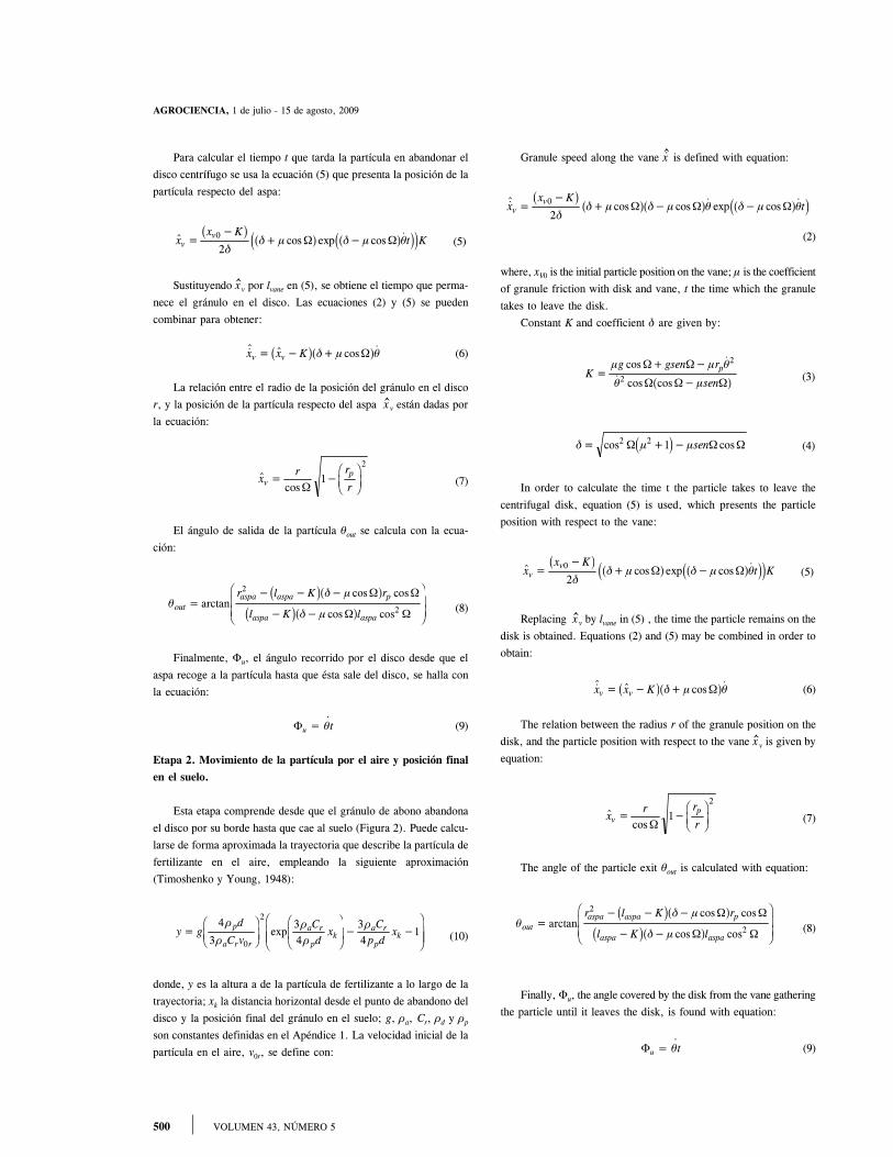
Etapa 2. Movimiento de la partícula por el aire y posición final

en el suelo.

Esta etapa comprende desde que el gránulo de abono abandona

el disco por su borde hasta que cae al suelo (Figura 2). Puede calcu-

larse de forma aproximada la trayectoria que describe la partícula de

fertilizante en el aire, empleando la siguiente aproximación

(Timoshenko y Young, 1948):

y gd

C v

C

dx

C

p dx

p

a r r

a r

pk

a r

pk=

FHG

IKJFHG

IKJ

− −FHGG

IKJJ

4

3

3

4

3

41

0

2ρ

ρ

ρ

ρ

ρexp (10)

donde, y es la altura a de la partícula de fertilizante a lo largo de la

trayectoria; xk la distancia horizontal desde el punto de abandono del

disco y la posición final del gránulo en el suelo; g, ρa, Cr, ρd y ρp

son constantes definidas en el Apéndice 1. La velocidad inicial de la

partícula en el aire, v0r, se define con:

Granule speed along the vane x. is defined with equation:

&$ cos cos & exp cos &xx K

tvv

=−

+ − −0

2

b g a fa f a fd iδ

δ µ δ µ θ δ µ θΩ Ω Ω

(2)

where, xV0 is the initial particle position on the vane; µ is the coefficient

of granule friction with disk and vane, t the time which the granule

takes to leave the disk.

Constant K and coefficient δ are given by:

Kg gsen r

sen

p=

+ −

−

µ µ θ

θ µ

cos &

& cos cos

Ω Ω

Ω Ω Ω

2

2 a f (3)

δ µ µ= + −cos cos2 2 1Ω Ω Ωd i sen (4)

In order to calculate the time t the particle takes to leave the

centrifugal disk, equation (5) is used, which presents the particle

position with respect to the vane:

$ cos exp cos &xx K

t Kvv

=−

+ −0

2

b g a f a fd ie jδ

δ µ δ µ θΩ Ω (5)

Replacing x v by lvane in (5) , the time the particle remains on the

disk is obtained. Equations (2) and (5) may be combined in order to

obtain:

&$ $ cos &x x Kv v= − +b ga fδ µ θΩ (6)

The relation between the radius r of the granule position on the

disk, and the particle position with respect to the vane x v is given by

equation:

$

cosx

r r

rv

p= −

FHGIKJΩ

12

(7)

The angle of the particle exit θout is calculated with equation:

θδ µ

δ µout

aspa aspa p

aspa aspa

r l K r

l K l=

− − −

− −

F

HGG

I

KJJarctan

cos cos

cos cos

2

2

c ha fc ha f

Ω Ω

Ω Ω(8)

Finally, Φu, the angle covered by the disk from the vane gathering

the particle until it leaves the disk, is found with equation:

Φu = θ.t (9)



v v v

v V

r m

m m u out

0 0 0

0 0

= −

= − + +cos π φ φ θb gc h (11)

donde, Vm es la velocidad del tractor; φ0 el ángulo inicial del gránulo

tomando como referencia 0° la dirección de avance del tractor; φu el

ángulo recorrido por el ángulo recorrido por el disco desde que el

aspa recoge a la partícula hasta que ésta sale del disco; φout es el

ángulo entre el vector velocidad y el vector radio en el extremo del

disco.

Las coordenadas cartesianas de la posición final del gránulo en

el suelo, xtot y ztot, se obtienen mediante trigonometría:

x x xA

z z z

tot fd

tot f

= +

= +

1

1

2m

(12)

Con el signo +− para los discos izquierdo (−) o derecho (+); Ad

es la distancia entre los centros de los discos; xf y zf son las coorde-

nadas de la posición de la partícula cuando abandona el disco. Den-

tro de estas ecuaciones, x1 y z1 se definen con:

x x x sen

z x sen x sen

k out u k out u

k out u k out u

1 0 0

1 0 0

2

2

= + + + ±FHG

IKJ

= + + + ±FHG

IKJ

cos cos cos

cos sin

θ θπ

θ θπ

Φ Φ Φ Φ

Φ Φ Φ Φ

b g

b g (13)

con ± para cada sentido de giro en el de las agujas del reloj (+)

o en el contrario (−).

Etapa 3. Obtención de coeficientes.

El perfil de distribución de una abonadora es la masa de fertili-

zante que hay en una franja perpendicular a su trayectoria. Para

obtener este perfil el programa divide el eje horizontal en intervalos

de 1 m y determina la masa total de abono en cada intervalo; con

Figura 2. Trayectoria de la partícula en el aire.Figure 2. Particle trajectory in the air.

Discos cónicos

Centro de la abonadora

Trayectoria del gránulo por el aire

VvVv V0

Ω

VH

X (0,0)

Y Phase 2: Particle movement in the air and final position on the

soil.

This phase covers the trajectory since the fertilizer granule leaves

the disk by its rim until it falls to the soil (Figure 2). The trajectory

which the fertilizer particle describes in the air may be calculated

approximately employing the following equation (Timoshenko and

Young, 1948):

y gd

C v

C

dx

C

p dx

p

a r r

a r

pk

a r

pk=

FHG

IKJFHG

IKJ

− −FHGG

IKJJ

4

3

3

4

3

41

0

2ρ

ρ

ρ

ρ

ρexp (10)

where, y is fertilizer particle height along the trajectory; xk is the

horizontal distance from the exit point of the disk and the final

granule position on the soil; g, ρa, Cr, ρd and ρp are constants defined

in Appendix 1. Initial particle speed in the air, v0r, is defined with:

v v v

v V

r m

m m u out

0 0 0

0 0

= −

= − + +cos π φ φ θb gc h (11)

where, Vm is the tractor speed; φ0 is the initial granule angle, taking

0° tractor advance direction as reference; φu the angle covered by

the angle covered by the disk, since the vane gathers the particle

until it comes off the disk; φout is the angle between the disk vector

and the radius vector at the disk rim.

The Cartesian coordinates of the final granule position on the

soil, xtot and zto, are obtained by means of trigonometry.

x x xA

z z z

tot fd

tot f

= +

= +

1

1

2m

(12)

With the sign+− for left disks (−) or right disks (+); Ad is the

distance between disk centers; xf and zf are the coordinates of particle

position when leaving the disk. Within these equations, x1 and z1 are

defined with:

x x x sen

z x sen x sen

k out u k out u

k out u k out u

1 0 0

1 0 0

2

2

= + + + ±FHG

IKJ

= + + + ±FHG

IKJ

cos cos cos

cos sin

θ θπ

θ θπ

Φ Φ Φ Φ

Φ Φ Φ Φ

b g

b g (13)

with ± for each turn sense of the hands of the clock (+), or

contrary to it (−).

Phase 3: Obtaining of coefficients.

The fertilizer distribution profile is the fertilizer mass existing

in a strip perpendicular to its trajectory. In order to obtain this

profile, the program divides the horizontal axis into intervals of 1 m



esas masas construye una gráfica obteniendo el perfil de distribu-

ción.

El CV de la densidad de fertilizante en el terreno, denominado

simplemente como CV en el ámbito de la distribución de fertilizan-

te, se obtiene con el perfil de distribución, y mide la uniformidad en

la distribución de fertilizante para cada valor de separación entre

pasadas; esta uniformidad es mayor cuanto menor es este coeficien-

te. En su cálculo para cada posible distancia entre pasadas, el pro-

grama superpone el perfil de distribución y determina la varianza

del perfil de distribución combinado. Se calcula el CV para esa

distancia con las fórmulas:

CX

X iN

X n

N

i

i N

var ,= =

−LNMOQP−

FHG

IKJ=

= −

∑σ

σ1002

2

0

1

donde (14)

donde, N es el ancho de trabajo de la abonadora; X[i] la masa de

partículas que hay en cada metro una vez realizadas todas las pasa-

das; X−

[n] la masa de partículas por metro del perfil combinado.

La aplicación de optimización

Las mejores variables de la abonadora se buscan mediante va-

rias simulaciones donde se modifican los valores de las variables

que se optimizarán. Los valores iniciales de dichas variables se de-

nominan semillas. La aplicación desarrollada puede realizar una si-

mulación y lanzar nuevas simulaciones con nuevos parámetros obte-

nidos en función de los datos provenientes de simulaciones anterio-

res. El usuario debe indicar al programa las variables para optimizar,

su intervalo de variación, y el criterio de optimización, ya que se

pueden optimizar de una a varias variables. Los parámetros de las

nuevas optimizaciones se buscan con el método del gradiente y los

siguientes pasos:

1) Se genera aleatoriamente un valor inicial para cada variable que

se optimizará. Se denomina semilla al conjunto de estos valores.

2) Se modifican ligeramente los valores de las variables de la semi-

lla inicial sumando y restando unos pasos, y se obtiene un grupo

formado por el conjunto de valores de la semilla, así como los

conjuntos de valores próximos a la semilla.

3) Se calculan con el simulador los CV correspondientes a cada

conjunto de valores.

4) Con el criterio de optimización se comparan los coeficientes

para encontrar el conjunto de valores con el mejor CV, de acuerdo

con el criterio de optimización fijado.

5) El proceso se repetirá partiendo de esos nuevos valores.

El programa continúa ejecutándose hasta un momento donde

todas las modificaciones con pequeños aumentos de las variables a

optimizar, producen un peor CV; así habrá un máximo local del

CV. Dado que el proceso se repite con nuevas semillas, es muy alta

la probabilidad de obtener el mejor CV o CV óptimo.

and determines the total fertilizer mass in each interval; with these

masses, a graph is constructed obtaining the distribution profile.

The CV of fertilizer density in the land, simply named CV in

the fertilizer distribution area, is acquired with the distribution profile,

and measures the uniformity in fertilizer distribution for each

separation value between rows; this uniformity is the greater, the

smaller the coefficient is. In its calculation for each possible distance

between rows, the program sums the distribution profiles of all passes

and determines the variance of the combined distribution profile.

The CV for this distance is calculated with the formulas:

CX

X iN

X n

N

i

i N

var ,= =

−LNMOQP−

FHG

IKJ=

= −

∑σ

σ1002

2

0

1

donde (14)

where, N is the work width of the fertilizer machine; X [i] is the

particle mass in each meter, once all the rows are finished; X−

[n]

the particle mass per meter of combined profile.

Application of optimization

The best variables of the fertilizing machine are searched by

means of various simulations where the variable values to be optimized

are modified. The initial values of such variables are called seeds.

The developed application may conduct a simulation and launch new

simulations with new parameters obtained according to the data

coming from previous simulations. The user has to indicate the

variables to optimize the program, its variation interval, and the

optimization criterion, since it is possible to optimize from one to

several variables. The parameters of the new optimizations are

searched using the gradient method and taking the following steps:

1) Randomly an initial value is generated for each variable that will

be optimized. The set of these initial values is called seeds.

2) Initial seed variable values are slightly modified, adding and

subtracting some steps, and a group formed by the set of seed

values is obtained, as well as the sets of values nearest to the

seed.

3) The CV corresponding to each set of values is calculated with the

simulator.

4) Based on the optimization criterion, the coefficients for finding

the set of values with the best CV are compared according to the

fixed optimization criterion.

5) The process will be repeated starting from these new values.

The program continues being executed until the moment when

all the modifications with small increments of the variables to optimize

produce worse CV, thus there will be a local maximum of CV.

Since the process is repeated with new seeds, the probability of

obtaining better, or the best CV is very high.

The optimization criteria serve to define how to select the best

CV, together with an optimization limit chosen by the user. The



Los criterios de optimización sirven para definir cómo elegir al

mejor CV, junto con un límite de optimización elegido por el usua-

rio. La aplicación busca en cada CV la máxima distancia entre pasa-

das que cumple el criterio y puede encontrar:

1) El último valor del CV que sea inferior al límite de optimización.

2) El primer valor del CV que sea superior al límite de optimización.

3) El último grupo de cinco valores consecutivos del CV que sean

inferiores al límite de optimización.

4) El primer grupo de cinco valores consecutivos del CV con un

elemento superior al límite de optimización.

Un problema del optimizador es que sólo encuentra máximos

locales debido a que la aplicación informática busca el mejor CV

comparando valores próximos entre sí, y por tanto los máximos que

encontrará serán máximos locales. En la Figura 3 se muestra que

hay máximos locales en una optimización donde se varían única-

mente dos variables: el ángulo de las aspas y la velocidad angular a

la que giran los discos.

La solución a este problema es realizar varias búsquedas con

muchas semillas para aumentar la probabilidad de encontrar un máxi-

mo absoluto. Realizar búsquedas con varias semillas, aunque sin una

certeza absoluta de llegar al máximo absoluto, aumenta considera-

blemente la probabilidad de llegar a éste, o se llegará a un máximo

local con un buen CV.

RESULTADOS Y DISCUSIÓN

Planteamiento

Un ensayo realizado con la aplicación informáticaconsistió en optimizar un equipo de abonado con ca-racterísticas similares a modelos de bajo coste que es-tán en el mercado y con discos pequeños y revolucio-nes de giro bajas-medias. El modelo a optimizar poseelas siguientes características:

1) La abonadora posee dos discos distribuidores concentros separados 0.7 m.

2) El radio de cada disco es 0.3 m.3) La velocidad de rotación de los discos es 26.67 p

rad·s−1 (800 rpm).4) El ángulo que forman los discos con la horizontal

W es 0.0873 rad.5) Los discos están a una altura de 1.5 m respecto al

punto de salida de la partícula en el disco.6) La velocidad de avance del tractor es 3 m·s−1.

El fertilizante usado en la simulación fue KemiraCAN 27 % N, que según Dintwa et al. (2004b), tienedensidad global ρb= 1035 kg·m−3, densidad de la par-tícula 1800 kg·m−3, y coeficiente de fricción con elplato de acero de µ=0.3.

Figura 3. Máximos locales en una optimización.Figure 3. Local maxima in an optimization

Dista

ncia

ent

re p

asad

as (m

) 45

40

35

30

25

20

15900

800700

600500

400

Velocidad angular (rev/min)20

15

Ángulo de

las aspa

s (°)105

0

application searches in each CV the largest distance between rows

which the criterion fulfills and can find:

1) The last CV value being inferior to the optimization limit.

2) The first CV value being higher than the optimization limit.

3) The last group of five consecutive CV values being below the

optimization limit.

4) The first group of five consecutive CV values with an element

above the optimization limit.

One problem of the optimizer is that it only finds local maxima,

due to the fact that the computerized application seeks the best CV,

comparing the nearest values among each other, and therefore the

maxima that it may find will be local maxima. Figure 3 shows that

there are local maxima in an optimization where only two variables

are altered, the vane angle and the angular speed of discs.

The solution of this problem consists in carrying out several

searches with many seeds in order to increase the probability to find

an absolute maximum. Conducting searches with various seeds, even

though without absolute certainty to reach the absolute maximum

considerably increases the probability to reach it or to arrive at a

local maximum with a good CV.

RESULTS AND DISCUSSION

Approach

A trial carried out with computerized applicationconsisted in optimizing fertilizing equipment withcharacteristics similar to low-cost models being on themarket and with small disks and revolutions of low tomedium turn. The model to be optimized has thefollowing characteristics:



Las partículas poseen forma esférica y su coefi-ciente de resistencia al aire es Cr=0.44 (Mennel yReece, 1963). El tamaño de los cedazos usados parahallar la granulometría de las partículas fue 1, 1.4, 2,2.4, 2.8, 3.4, 4 y 5.6 mm; el porcentaje de la masa departículas en cada cedazo fue 0, 0, 0.1, 2.4, 12.7,38.8, 35.6, 10.4 y 0. Ninguna partícula atravesó losdos últimos cedazos, y ninguna se quedó sobre el ce-dazo con la malla más gruesa.

El orificio de alimentación tiene forma rectangular,el tractor con la abonadora se mueve a una velocidadde 2.78 m·s−1 y la densidad del aire es 1.2 kg·m−3.

Las variables optimizadas en este estudio son lascuatro que definen el orificio de alimentación: abcisa yordenada del centro de la apertura (xcentro e ycentro); y lalongitud de los lados horizontales y verticales de laabertura (xlado e ylado). También se optimiza el ángulode las aspas.

El criterio de optimización en este estudio es eltercero de los que posee la aplicación, es decir, elprograma buscará el último grupo de cinco valoresconsecutivos del CV menores al límite de optimización.El límite de optimización se fijó en 12 %, por ser unvalor admisible para el CV en aplicaciones agrícolasde fertilización.

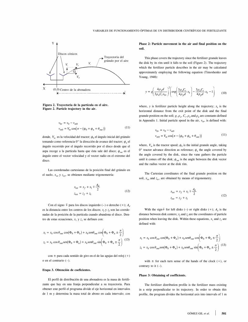
RESULTADOS

En el Cuadro 1 se muestran los resultados obteni-dos después de una serie de optimizaciones con la apli-cación desarrollada. El mejor resultado se muestra enla primera fila del Cuadro 1 por cumplir el criterio deoptimización a una distancia entre pasadas de 22 m,mientras que el resto lo cumplen sólo para distanciasentre pasadas de 20 m.

Para esta anchura de 22 m, algunas de las gráficasque calcula el simulador se muestran en las Figuras 4,5, 6 y 7. En la Figura 4 se muestra la trayectoriacalculada en 150 gránulos de fertilizante que caen enel disco distribuidor. En la Figura 5 se muestra ladistribución sobre el terreno de las partículas de ferti-lizante, cuando la máquina abonadora no se desplaza.

Cuadro 1. Variables óptimas obtenidas tras la optimización.Table 1. Optimal variables obtained after optimization.

Distancia Ángulo de xcentro ycentro xlado yladoentre las aspaspasadas (m) (rad)

(m) (m) (m) (m)

22 0 0.19 −0.03 0.16 0.1120 0.035 0.2 −0.02 0.12 0.1520 0.209 0.19 −0.01 0.14 0.1520 0.140 0.19 −0.02 0.14 0.12 Figura 4. Trayectoria de las partículas en el disco izquierdo.

Figure 4. Particle trajectory on the left disk

Trayectorias de las partículas en el disco izquierdo

30

30

25

20

15

5

5(cm)

(cm)

−30

−30

−25

−25

−20

−20

−15

−15

−10

−10

−5−5

15 20 25

1) The fertilizer machine has two distributor disks,with centers separated at 0.7 m.

2) The radius of each disk is 0.3 m.3) Disk rotation speed is 26.67 p rad·s−1 (800 rpm).4) The angle formed by the disks with the horizontal

W is 0.0873 rad.5) The disks are at 1.5 m height with respect to the

particle exit point on the disk.6) Tractor forward speed is 3 m·s−1.

The fertilizer used in the simulation was KemiraCAN 27% N, which according to Dintwa et al. (2004b)has global density ρb=1035 kg·m−3, particle density1800 kg·m−3, and friction coefficient with the steelplate of µ=0.3.

The particles are spherical and their resistancecoefficient to air is Cr=0.44 (Mennel and Reece, 1963).The size of the sieves utilized to find particle granulometrywas 1, 1.4, 2, 2.4, 2.8, 3.4, 4, and 5.6 mm; particlemass percentage in each sieve was 0, 0, 0.1, 2.4, 12.7,38.8, 35.6, 10.4, and 0. None of the particles wentthrough the last two sieves, and none of them stayedon the sieve with the thickest net.

The supply opening orifice is rectangular, the tractorwith the fertilizer machine moves at a speed of 2.78 m·s−1, and air density is 1.2 kg·m−3.

The optimized variables in this study are the fourthat define the supply opening: abscissa and ordinateof the opening center (xcenter and ycenter), and lengthof the horizontal and vertical sides of the opening (xsideand yside). The vane angle also is optimized.



Figura 5. Distribución en el suelo de las partículas de fertilizante.Figure 5. Fertilizer particle distribution on soil.

14.5

Posición de las partículas en el suelo

Eje x (m)

14.013.513.012.512.011.511.010.510.09.59.08.58.07.57.06.56.0

Eje

y (m

)

5.55.04.54.03.53.02.52.01.51.0

−15 −14 −13−12−11 −10 −9 −8 −7 −6 −5 −4 −3 −2 −1 0 1 2 3 4 5 6 7 8 9 10 11 12 13 14 15

Figura 6. Perfil de distribución.Figure 6. Distribution profile.

1.00

Patrón de distribución transversal normalizado

Eje x (m)

0.950.900.850.800.750.700.650.600.550.500.450.400.350.300.250.200.15

Eje

y (m

)

0.100.050.00

−15−17−16 −14−13−12−11−10 −9 −8 −7 −6 −5 −4 −3 −2 −1 0 1 2 3 4 5 6 7 8 9 10 11 12 13 14 15 16 17

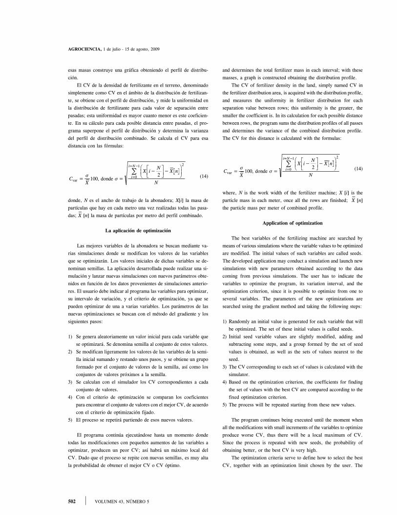
El perfil de distribución del equipo de abonado semuestra en la Figura 6, y el CV de la distribución enida y vuelta en la Figura 7.

The optimization criterion in this study is the thirdone of the application, in other words, the programwill search the last group of five consecutive CV values

14.5

Posición de las partículas en el suelo

Eje x (m)

14.013.513.012.512.011.511.010.510.09.59.08.58.07.57.06.56.0

Eje

y (m

)

5.55.04.54.03.53.02.52.01.51.0

−15 −14 −13−12−11 −10 −9 −8 −7 −6 −5 −4 −3 −2 −1 0 1 2 3 4 5 6 7 8 9 10 11 12 13 14 15

1.00

Patrón de distribución transversal normalizado

Eje x (m)

0.950.900.850.800.750.700.650.600.550.500.450.400.350.300.250.200.15

Eje

y (m

)

0.100.050.00

−15−17−16 −14−13−12−11−10 −9 −8 −7 −6 −5 −4 −3 −2 −1 0 1 2 3 4 5 6 7 8 9 10 11 12 13 14 15 16 17

El perfil de distribución del equipo de abonado semuestra en la Figura 6, y el CV de la distribución enida y vuelta en la Figura 7.

The optimization criterion in this study is the thirdone of the application, in other words, the programwill search the last group of five consecutive CV values

Figura 6. Perfil de distribución.Figure 6. Distribution profile.



50484644

Coeficiente de variación de ida y vuelta

424038363432302826242220181614121086420

0 1 2 3 4 5 6 7

Distancia (m)

8 9 10 11 12 13 14 15 16 17 18 19 20 21 22 23 24 25 26 27 28 29 30 31 32 34 3533

Figura 7. Coeficiente de variación ida y vuelta.Figure 7. Variation coefficient coming and going.

CONCLUSIONES

Los valores óptimos de las variables de funciona-miento obtenidos analíticamente tienen CV similares alos de marcas conocidas de equipos de abonado. Losmodelos SULKY DX Prisma, AMAZONE ZA-X, oKUHN AXIS tienen características de disco similaresen tamaño y velocidad de rotación, y permite anchosmáximos de trabajo de 24, 18, y 28 m.

Obtener experimentalmente estos resultados en unaestación de ensayo es una tarea que exige mucho tra-bajo y recursos, mientras que con la aplicación desa-rrollada se obtiene resultados rápidamente. La misiónde la estación de ensayo sería ajustar finamente losparámetros obtenidos con esta aplicación.

LITERATURA CITADA

Dintwa, E., P. Van Liedekerke, R. Olieslagers, E. Tijkens, and H.Ramon. 2004a. Model for simulation of particle flow on acentrifugal fertiliser spreader. Biosystems Eng. 87(4): 407-415.

Dintwa, E., E. Tijskens, R. Olieslagers, J. De Beardemaeker, andH. Ramon. 2004b. Calibration of a spinning disc spreadersimulation model for accurate site-specific fertiliser application.Biosystems Eng. 88(1): 49-62.

Mennel, R. M., and A. R. Reece. 1963. The theory of the centrifugaldistributor III: particle trajectories. J. Agric. Eng. Res. 8(1):78-84.

Olieslagers, R., H. Ramón, and J. de Baeremaeker. 1996. Calculationof fertilizar distribution patterns from a spinning disc spreader bymeans of a simulation model. J. Agric. Eng. Res. 63: 137-152.

smaller than the optimization limit. The optimizationlimit was fixed at 12%, because of being an admissiblevalue for CV in agricultural fertilizer applications.

RESULTS

The results obtained after a series of optimizationswith developed application are shown in Table 1. Thebest result is shown in the first line of Table 1 forfulfilling the optimization criterion at a distance betweenrows of 22 m, while the rest fulfills it only for distancesbetween rows of 20 m.

For this width of 22 m, some of the graphs whichthe simulator calculates are shown in Figures 4, 5, 6,and 7. The trajectory calculated in 150 fertilizer granuleswhich fall on the distributor disk is shown in Figure 4.In Figure 5, the fertilizer particle distribution on theland is presented, when the machine does not movefrom its place. The distribution profile of the fertilizerequipment is shown in Figure 6, and the distributiongo and return CV in Figure 7.

CONCLUSIONS

The best values of the operation variables analyticallyobtained have CV similar to those of well-knownfertilizer equipment trade marks. SULKY DX Prisma,AMAZONE ZA-X, or KUHN AXIS models have disk



characteristics, similar in size and rotation speed, andallow maximum work width of 24, 18, and 28 m.

Obtaining these results experimentally at a test siteis a task which demands a lot of labor and resources,whereas using developed application, results areobtained quickly. The mission of the test site wouldbe, artfully adjusting the obtained parameters with thisapplication.

Grift, T.E., and J. W. Hofstee. 2002. Testing an online spreadpattern determination sensor on a broadcast fertilizer spreader.T. of the Asabe 45(3): 561–567.

Swisher, D.W., S. C. Borgelt, and K. A. Sudduth. 2002. Opticalsensor for granular fertilizer flow rate measurement. T. of theAsabe 45(4): 881–888.

Tissot, S., O. Miserque, O. Mostade, B. Huyghebaert, and J. P.Destain. 2002. Uniformity of N-fertilizer spreading and risk ofground water contamination. Irrig. and Drainage 51(1): 17-24.

Timoshenko, S., and D.H. Young. 1984. Advanced Dynamics.McGraw-Hill Book Co., Inc. New York, NY. 1948 p.

Villette, S., F. Cointault, E. Pirón, and B. Chopinet. 2005. Centrifugalspreading: an analytical model for the motion of fertiliser particleson a spinning disc. Biosystems Eng. 92(2): 157-164. Enesad,UMR Cemagref-Enesad, Dsi-Lgap, Bp 87999, 21079 DijonCedex, France.



Apéndice (Olieslagers et al., 1996)Appendix (Olieslagers et al., 1996)

Ad Distancia entre los centros de los discos, m.

Cr Coeficiente de resistencia del aire.

Cvar Coeficiente de variación de la abonadora, %.

d Diámetro de una partícula, m.

g Aceleración de la gravedad, m s−2.

N Ancho de trabajo de la abonadora, m.

laspa Longitud de las aspas, m.

O Punto en el eje rotacional del disco.

Ov Proyección de O en el eje del aspa.

r Radio de la posición del gránulo en el disco res-pecto del centro del mismo, m.

rp Radio del círculo tangente a las aspas, m.

raspa Radio del disco .

t Tiempo, s.

vH Componente horizontal de v0, m s−1.

Vm Velocidad de la máquina abonandora, m s−1.

vR Componente radial de vH, m s-1.

vT Componente tangencial de vH, m s-1.

vy Componente vertical de v0, m s-1.

v0 Velocidad de la partícula cuando abandona el dis-co, m s-1.

v0r Velocidad inicial de la partícula en el aire, m s-1.

xf Abcisa del punto por el que la partícula abandonael disco, m.

xk Distancia entre el punto de abandono del disco yla posición final del gránulo en el suelo, m.

xtot Abcisa de la posición final de la partícula en elsuelo, m.

Ad Distance between disk centers, m.

Cr Air resistance coefficient.

Cvar Fertilizer variation coefficient, %.

d Particle diameter, m.

g Gravity acceleration, m s−2.

N Fertilizer machine work width, m.

laspa Vane length, m.

O Point on disk rotation axis.

Ov O projection on vane axis.

r Granule position radius on the disk with respectto its center, m.

rp Radius from the tangent circle to vanes, m.

raspa Disk radius.

t Time, s.

vH v0 Horizontal component, m s−1.

Vm Fertilizer machine speed, m s−1.

vR vH Radial component, m s−1.

vT vH Tangential component, m s−1.

vy v0 Vertical component, m s−1.

v0 Particle speed at leaving disk, m s−1.

v0r Initial particle speed in the air, m s−1.

xf Abscissa of particle exit point on disk, m.

xk Distance between exit point of disk and finalposition of granule on soil, m.

xtot Abscissa of particle final position on soil, m.

x v Abscissa of granule on vane with respect to Ov, m.



x v Abcisa del gránulo en el aspa respecto de Ov, m.

x v Velocidad de la partícula en el aspa, m s−1.

xv0 Posición inicial de la partícula en el aspa, m.

y Altura de la partícula en cada punto de la trayec-toria, m.

zf Ordenada del punto por el que la partícula aban-dona el disco, m.

ztot Ordenada de la posición final de la partícula en elsuelo, m.

αlv Ángulo de inclinación de las aspas, rad.

θout Ángulo entre el vector velocidad y el vector radioen el extremo del disco, rad.

θ.

Velocidad angular del disco, rad s−1.

µ Coeficiente de fricción entre la partícula y el dis-co o aspas.

ρa Densidad del aire, g m-3.

ρp Densidad de la partícula, g m−3.

σ Desviación típica del perfil de distribución.

Φ0 Angulo de la posición inicial de la partícula en eldisco, rad.

Φu Ángulo recorrido por la partícula en su movimientopor el disco, rad.

Ω Ángulo entre el aspa y el plano horizontal, rad.

x v Particle speed on vane, m s-1.

xv0 Initial particle position on vane, m.

y Particle height at each trajectory point, m.

zf Ordinate of particle exit point on disk, m.

ztot Ordinate of particle final position on soil, m.

αlv Inclination angle of vanes, rad.

θout Angle between speed vector and radius vector atdisk rim, rad.

θ.

Angular disk speed, rad.

µ Friction coefficient between particle and disk orvanes.

ρa Air density, g m-3.

ρp Particle density, g m-3.

σ Typical deviation of distribution profile.

Φ0 Initial position angle of particle on disk, rad.

Φu Angle covered by particle in its movement ondisk, rad.

Ω Angle between vane and the horizontal plane,rad.

Redalyc.ESTIMACIÓN ANALÍTICA DE LAS … · coeficiente de variación, es fundamental para una...

Documents

Transcript of Redalyc.ESTIMACIÓN ANALÍTICA DE LAS … · coeficiente de variación, es fundamental para una...