Uso de radio mobile para el calculo de coberturas radio en dispositivos de comunicacion inalambrica
Radio Mobile
Prácticas de Radioenlaces
Profesores: Almudena Suárez Rodríguez
Álvaro Álvarez Vázquez
Radio Mobile – Prácticas de Radioenlaces
- 1 -
Indice 1. Inicio y Especificaciones .......................................................................................... 3
1.1. Radio Mobile Data Sheet.................................................................................. 3
1.2. Arranque de la Aplicación................................................................................ 5
2. Radio Mobile Help Contents .................................................................................. 13
2.1. Main Menu ..................................................................................................... 13
2.1.1. File .......................................................................................................... 13
2.1.2. Edit ......................................................................................................... 15
2.1.3. View ....................................................................................................... 17
2.1.4. Tools ....................................................................................................... 18
2.1.5. Options ................................................................................................... 19
2.1.6. Window .................................................................................................. 19
2.1.7. Help ........................................................................................................ 20
2.2. How to ............................................................................................................ 20
2.2.1. Acquire elevation data ............................................................................ 20
2.2.2. Create a map picture ............................................................................... 21
2.2.3. Position units .......................................................................................... 23
2.2.4. Create a network..................................................................................... 24
2.2.5. Save and retrieve projects....................................................................... 28
2.2.6. Perform radio coverage .......................................................................... 28
2.2.7. Perform visual coverage ......................................................................... 29
2.2.8. Create an ADRG picture ........................................................................ 30
2.2.9. Import and scale user pictures ................................................................ 30
2.2.10. Create a flight animation ........................................................................ 31
2.2.11. Export profile data .................................................................................. 31
2.3. Basics.............................................................................................................. 32
2.3.1. Radio propagation model ....................................................................... 32
2.3.2. Radio link and system performance ....................................................... 33
2.3.3. 3D, panoramic, and stereoscopic views ................................................. 35
2.3.4. Geodesic, UTM, and MGRS coordinates............................................... 35
3. First example: the VHF coverage of my QTH ....................................................... 36
3.1. Acquire elevation database from the internet ................................................. 36
3.2. Extract elevation data and create a map picture ............................................. 37
3.3. Position my QTH............................................................................................ 38
3.4. Enter Network data......................................................................................... 39
Radio Mobile – Prácticas de Radioenlaces
- 2 -
3.5. VHF Radio coverage!..................................................................................... 42
4. Example 2: Introduction ......................................................................................... 43
4.1. Program setup................................................................................................. 43
4.2. Download my Zip file. ................................................................................... 44
4.3. Setting up RMW............................................................................................. 44
4.4. Notes............................................................................................................... 53
5. Advanced Guide ..................................................................................................... 55
5.1. Creating Extra Units ....................................................................................... 55
5.2. The Radio Link window................................................................................. 59
5.3. Radio Coverage Plots ..................................................................................... 61
6. Apendice................................................................................................................. 63
Radio Mobile – Prácticas de Radioenlaces
- 3 -
1. Inicio y Especificaciones
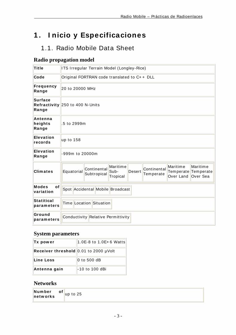
1.1. Radio Mobile Data Sheet
Radio propagation model Title ITS Irregular Terrain Model (Longley-Rice)
Code Original FORTRAN code translated to C++ DLL
Frequency Range 20 to 20000 MHz
Surface Refractivity Range
250 to 400 N-Units
Antenna heights Range
.5 to 2999m
Elevation records up to 158
Elevation Range -999m to 20000m
Climates Equatorial Continental Subtropical
Maritime Sub-Tropical
Desert Continental Temperate
Maritime Temperate Over Land
Maritime Temperate Over Sea
Modes of variation Spot Accidental Mobile Broadcast
Statitical parameters Time Location Situation
Ground parameters Conductivity Relative Permittivity
System parameters Tx power 1.0E-8 to 1.0E+6 Watts
Receiver threshold 0.01 to 2000 µVolt
Line Loss 0 to 500 dB
Antenna gain -10 to 100 dBi
Networks Number of networks up to 25
Radio Mobile – Prácticas de Radioenlaces
- 4 -
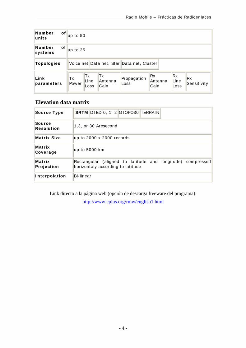
Number of units up to 50
Number of systems up to 25
Topologies Voice net Data net, Star Data net, Cluster
Link parameters
Tx Power
Tx Line Loss
Tx Antenna Gain
Propagation Loss
Rx Antenna Gain
Rx Line Loss
Rx Sensitivity
Elevation data matrix
Source Type SRTM DTED 0, 1, 2 GTOPO30 TERRAIN
Source Resolution 1,3, or 30 Arcsecond
Matrix Size up to 2000 x 2000 records
Matrix Coverage up to 5000 km
Matrix Projection
Rectangular (aligned to latitude and longitude) compressed horizontaly according to latitude
Interpolation Bi-linear
Link directo a la página web (opción de descarga freeware del programa):
http://www.cplus.org/rmw/english1.html
Radio Mobile – Prácticas de Radioenlaces
- 5 -
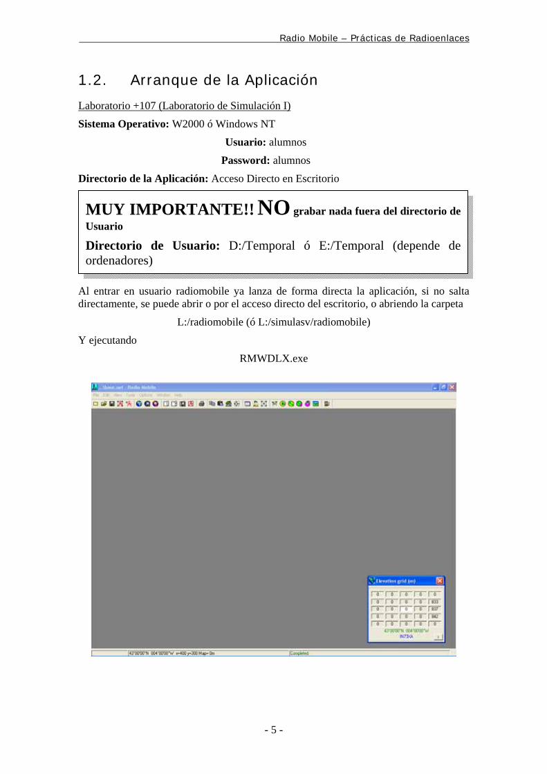
1.2. Arranque de la Aplicación
Laboratorio +107 (Laboratorio de Simulación I)
Sistema Operativo: W2000 ó Windows NT
Usuario: alumnos
Password: alumnos
Directorio de la Aplicación: Acceso Directo en Escritorio
Al entrar en usuario radiomobile ya lanza de forma directa la aplicación, si no salta directamente, se puede abrir o por el acceso directo del escritorio, o abriendo la carpeta
L:/radiomobile (ó L:/simulasv/radiomobile)
Y ejecutando
RMWDLX.exe
MUY IMPORTANTE!! NO grabar nada fuera del directorio de Usuario
Directorio de Usuario: D:/Temporal ó E:/Temporal (depende de ordenadores)
Radio Mobile – Prácticas de Radioenlaces
- 6 -
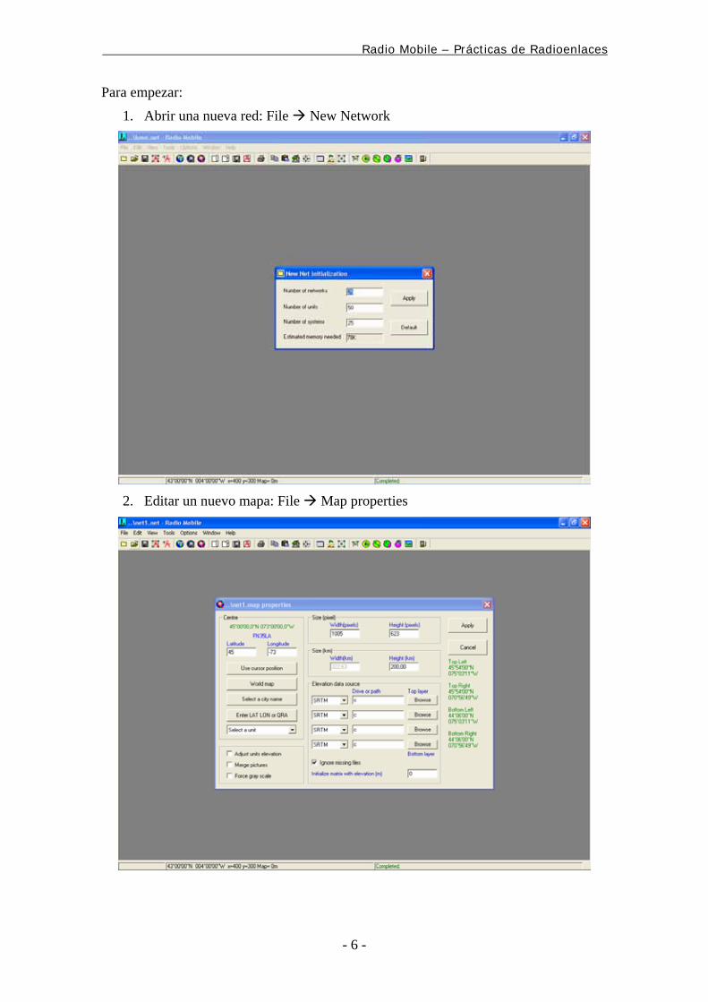
Para empezar:
1. Abrir una nueva red: File New Network
2. Editar un nuevo mapa: File Map properties
Radio Mobile – Prácticas de Radioenlaces
- 7 -
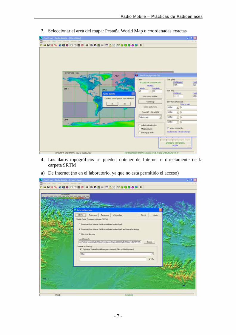
3. Seleccionar el area del mapa: Pestaña World Map o coordenadas exactas
4. Los datos topográficos se pueden obtener de Internet o directamente de la carpeta SRTM
a) De Internet (no en el laboratorio, ya que no esta permitido el acceso)
Radio Mobile – Prácticas de Radioenlaces
- 8 -
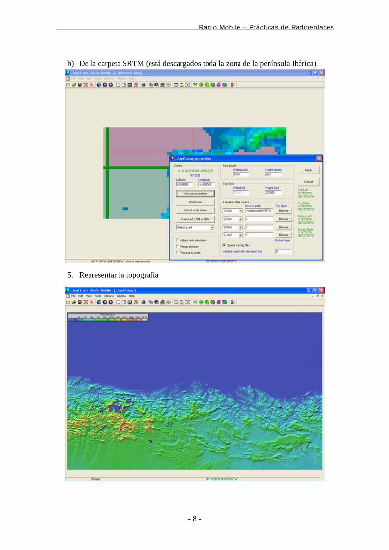
b) De la carpeta SRTM (está descargados toda la zona de la península Ibérica)
5. Representar la topografía
Radio Mobile – Prácticas de Radioenlaces
- 9 -
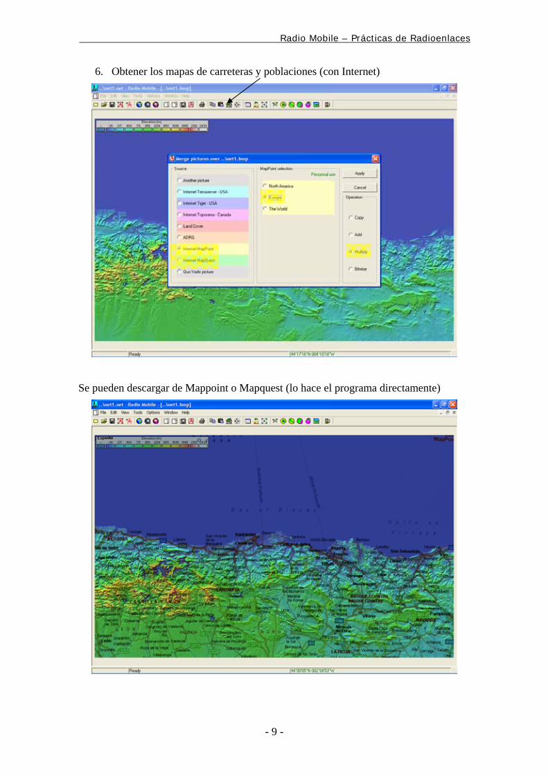
6. Obtener los mapas de carreteras y poblaciones (con Internet)
Se pueden descargar de Mappoint o Mapquest (lo hace el programa directamente)
Radio Mobile – Prácticas de Radioenlaces
- 10 -
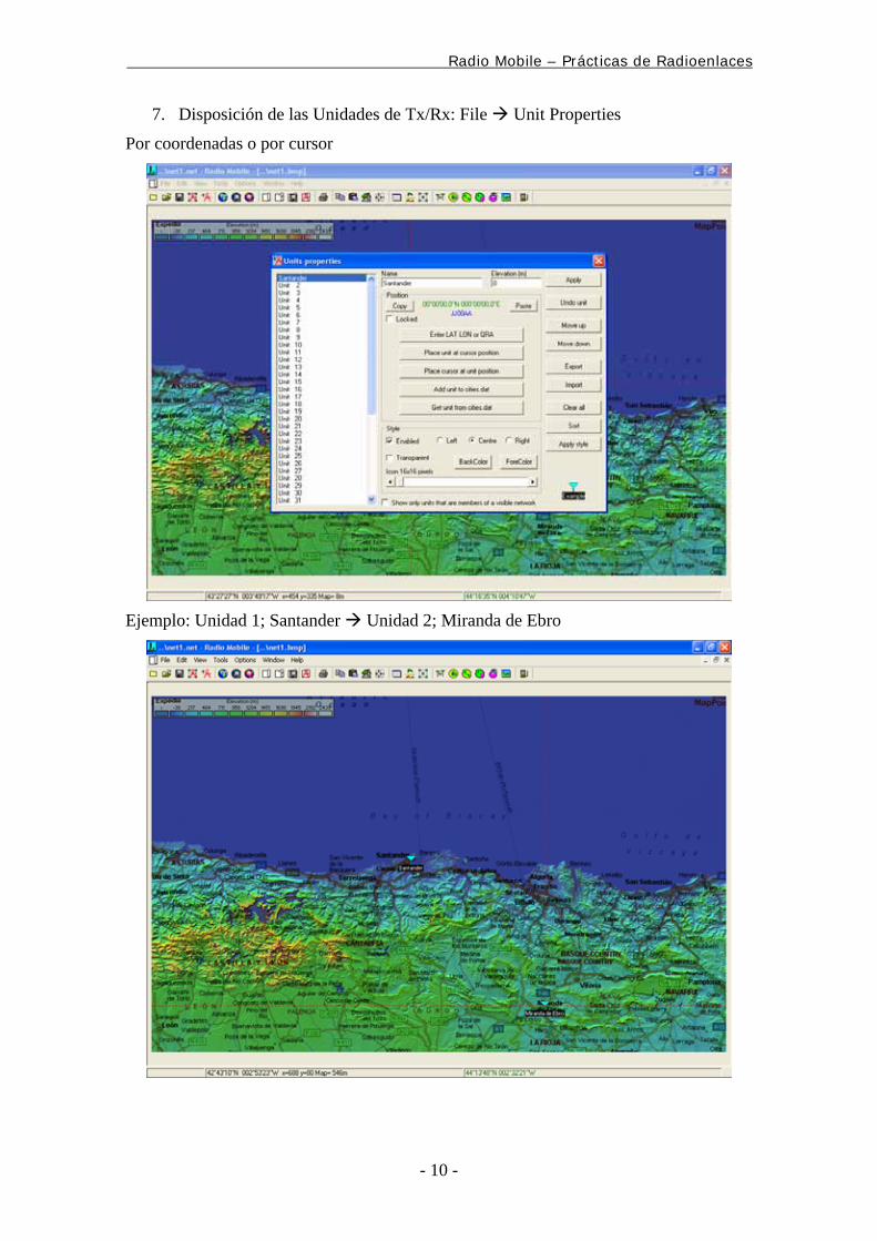
7. Disposición de las Unidades de Tx/Rx: File Unit Properties
Por coordenadas o por cursor
Ejemplo: Unidad 1; Santander Unidad 2; Miranda de Ebro
Radio Mobile – Prácticas de Radioenlaces
- 11 -
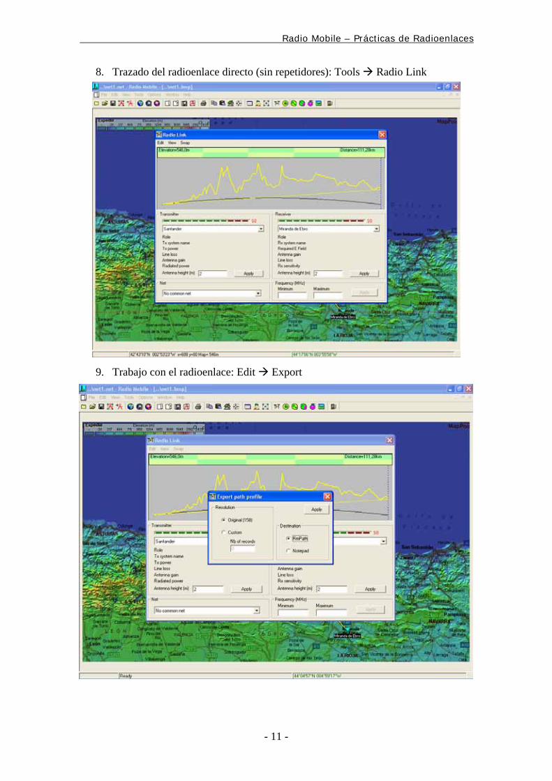
8. Trazado del radioenlace directo (sin repetidores): Tools Radio Link
9. Trabajo con el radioenlace: Edit Export
Radio Mobile – Prácticas de Radioenlaces
- 12 -
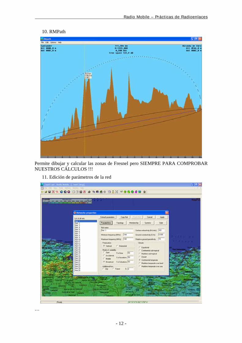
10. RMPath
Permite dibujar y calcular las zonas de Fresnel pero SIEMPRE PARA COMPROBAR NUESTROS CÁLCULOS !!!
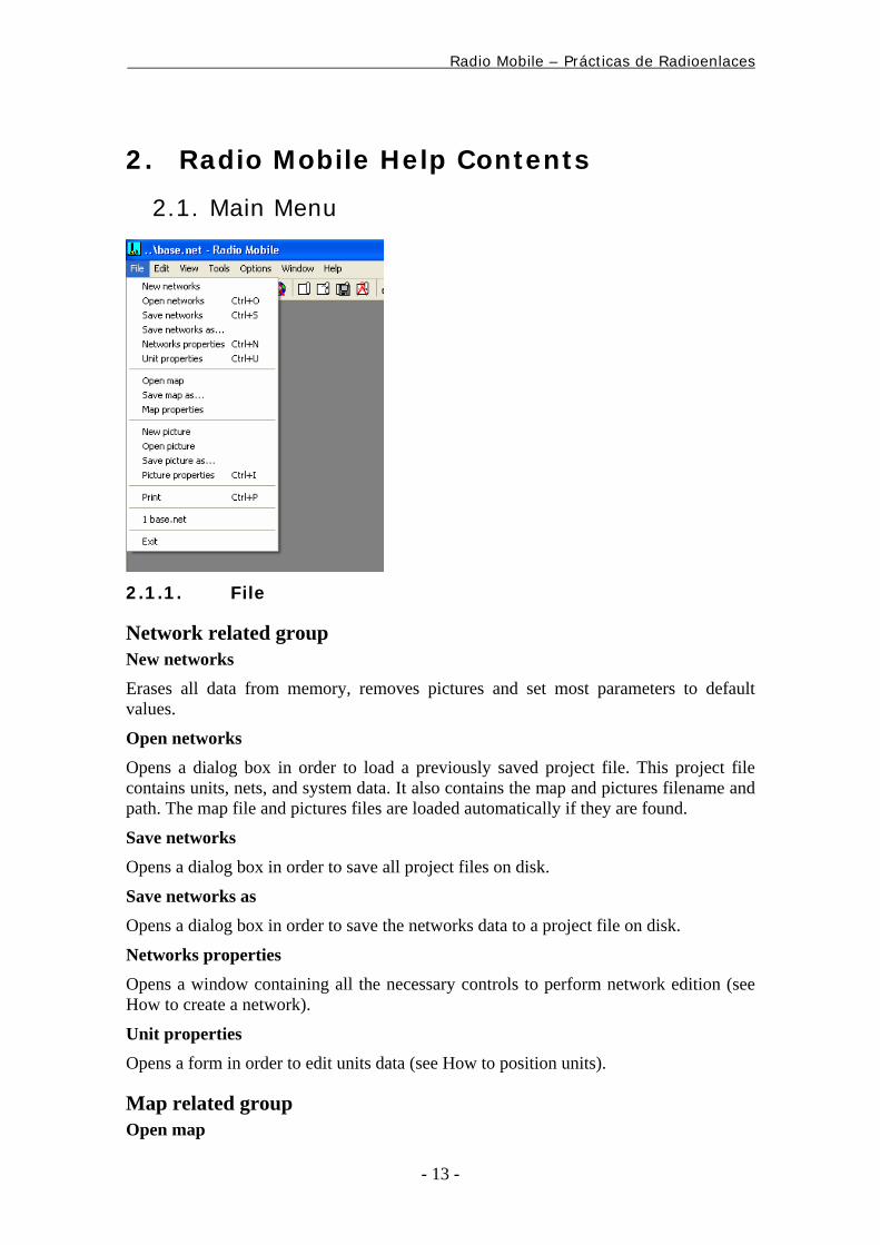
11. Edición de parámetros de la red
…
Radio Mobile – Prácticas de Radioenlaces
- 13 -
2. Radio Mobile Help Contents
2.1. Main Menu
2.1.1. File
Network related group New networks Erases all data from memory, removes pictures and set most parameters to default values.
Open networks
Opens a dialog box in order to load a previously saved project file. This project file contains units, nets, and system data. It also contains the map and pictures filename and path. The map file and pictures files are loaded automatically if they are found.
Save networks Opens a dialog box in order to save all project files on disk.
Save networks as Opens a dialog box in order to save the networks data to a project file on disk.
Networks properties Opens a window containing all the necessary controls to perform network edition (see How to create a network).
Unit properties Opens a form in order to edit units data (see How to position units).
Map related group Open map
Radio Mobile – Prácticas de Radioenlaces
- 14 -
Opens a dialog box in order to load a previously saved map file. The map file contains elevation data, and is normally associated with a bitmap picture file. Format conversion from earlier program version is performed when necessary.
Save map as Opens a dialog box in order to save map data into a file. The file, is named with the map name followed by a .MAP extension, and contains elevation data. Contrary to older version, the map picture will not be saved, because program allows multiple pictures per map. Each picture must be saved with the Save picture as command.
Map properties Opens a form in order to define the map coverage boundaries and select the elevation database (see How to acquire elevation data).
Picture related group New picture Opens the Picture properties form in order to create a new map picture.
Open picture Opens a dialog box in order to load a picture file from disk (BMP, GIF or JPEG). Picture files are associated with a properties file named with the picture followed by a .DAT extension. If the properties file is not found, the file is considered as a user picture that can be scaled manually (see Import and scale user pictures).
Save picture as Opens a dialog box in order to save a bitmap picture file (BMP only). Conversion to GIF or JPEG can be performed with another program to reduce the file size.
Picture properties Opens the appropriate form (Map, User or 3D type) that can be used to create or modify a map picture (see How to create a map picture
, How to create an ADRG picture, How to import and scale user pictures, and 3D, panoramic, and stereoscopic views).
Print related group Print Prints the active picture on a printer device. The picture is scaled and oriented to fit paper size.
Program related Files list Files shown are recent networks project files that can be recalled.
Exit
This command aborts program execution upon confirmation.
Radio Mobile – Prácticas de Radioenlaces
- 15 -
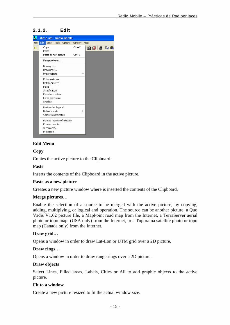
2.1.2. Edit
Edit Menu
Copy Copies the active picture to the Clipboard.
Paste Inserts the contents of the Clipboard in the active picture.
Paste as a new picture Creates a new picture window where is inserted the contents of the Clipboard.
Merge pictures… Enable the selection of a source to be merged with the active picture, by copying, adding, multiplying, or logical and operation. The source can be another picture, a Quo Vadis V1.62 picture file, a MapPoint road map from the Internet, a TerraServer aerial photo or topo map (USA only) from the Internet, or a Toporama satellite photo or topo map (Canada only) from the Internet.
Draw grid…
Opens a window in order to draw Lat-Lon or UTM grid over a 2D picture.
Draw rings… Opens a window in order to draw range rings over a 2D picture.
Draw objects Select Lines, Filled areas, Labels, Cities or All to add graphic objects to the active picture.
Fit to a window Create a new picture resized to fit the actual window size.
Radio Mobile – Prácticas de Radioenlaces
- 16 -
Rotate/Stretch Opens a window with rotation angle and stretch factor inputs that will be used to create a new picture on activation of the Apply command.
Flood Flood all map pixels surrounding cursor position that share the same elevation.
Stratification Opens a window used to color a stratum of elevation.
Elevation contour Opens a window used to draw a custom defined elevation contour interval.
Force gray scale Modify a picture to force a gray scale (useful for coverage background).
Shadow Modify a picture to draw shadows behind mountains.
Redraw last legend Redraw the last legend to a picture.
Distance scale Add a distance scale to a picture.
Corners coordinates Print the four corners lat-lon coordinates over a picture.
Fit map to picture/selection Opens the Map properties window in order to extract elevation data according to the picture or selection.
Fit map to units
Opens the Map properties window in order to extract elevation data in order to fit best all units in memory.
Orthorectify Draw a new picture that can then be adjusted to fit map exactly.
Projection
Draw a new picture according to a trapezoidal projection offering less distortion.
Radio Mobile – Prácticas de Radioenlaces
- 17 -
2.1.3. View
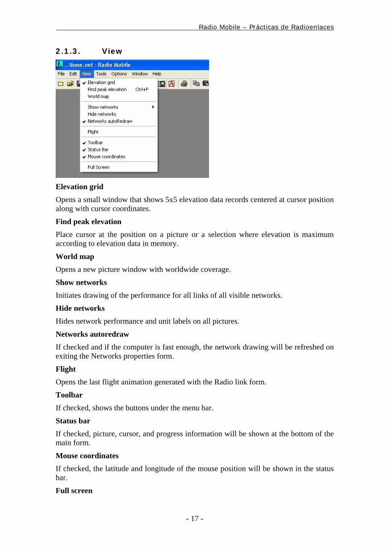
Elevation grid Opens a small window that shows 5x5 elevation data records centered at cursor position along with cursor coordinates.
Find peak elevation Place cursor at the position on a picture or a selection where elevation is maximum according to elevation data in memory.
World map Opens a new picture window with worldwide coverage.
Show networks Initiates drawing of the performance for all links of all visible networks.
Hide networks Hides network performance and unit labels on all pictures.
Networks autoredraw
If checked and if the computer is fast enough, the network drawing will be refreshed on exiting the Networks properties form.
Flight Opens the last flight animation generated with the Radio link form.
Toolbar
If checked, shows the buttons under the menu bar.
Status bar If checked, picture, cursor, and progress information will be shown at the bottom of the main form.
Mouse coordinates If checked, the latitude and longitude of the mouse position will be shown in the status bar.
Full screen
Radio Mobile – Prácticas de Radioenlaces
- 18 -
Maximize the active window to the maximum screen size. If the picture is larger than the screen, use keyboard arrows or mouse to move the picture.
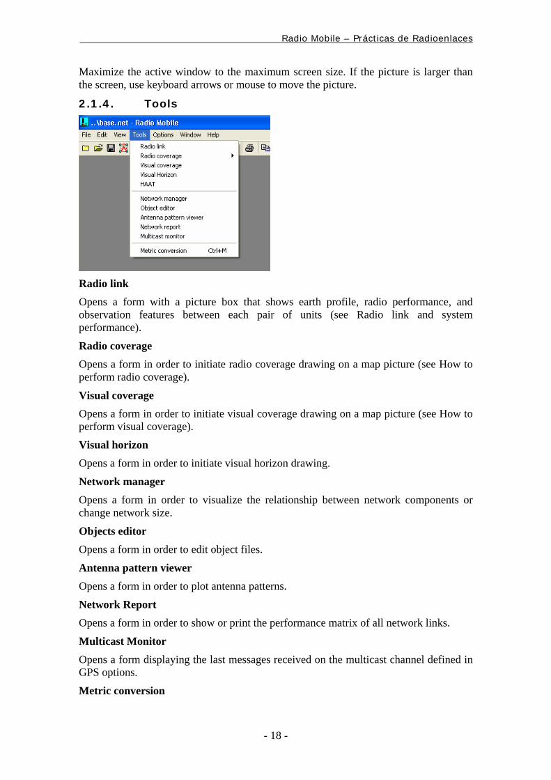
2.1.4. Tools
Radio link Opens a form with a picture box that shows earth profile, radio performance, and observation features between each pair of units (see Radio link and system performance).
Radio coverage Opens a form in order to initiate radio coverage drawing on a map picture (see How to perform radio coverage).
Visual coverage Opens a form in order to initiate visual coverage drawing on a map picture (see How to perform visual coverage).
Visual horizon Opens a form in order to initiate visual horizon drawing.
Network manager Opens a form in order to visualize the relationship between network components or change network size.
Objects editor
Opens a form in order to edit object files.
Antenna pattern viewer Opens a form in order to plot antenna patterns.
Network Report Opens a form in order to show or print the performance matrix of all network links.
Multicast Monitor Opens a form displaying the last messages received on the multicast channel defined in GPS options.
Metric conversion
Radio Mobile – Prácticas de Radioenlaces
- 19 -
Opens a form to perform metric conversion between two text boxes.
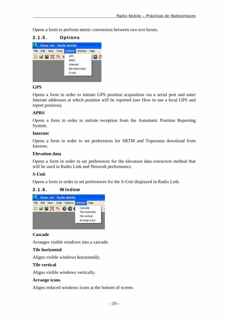
2.1.5. Options
GPS Opens a form in order to initiate GPS position acquisition via a serial port and enter Internet addresses at which position will be reported (see How to use a local GPS and report position).
APRS Opens a form in order to initiate reception from the Automatic Position Reporting System.
Internet Opens a form in order to set preferences for SRTM and Toporama download from Internet.
Elevation data Opens a form in order to set preferences for the elevation data extraction method that will be used in Radio Link and Network performance.
S-Unit Opens a form in order to set preferences for the S-Unit displayed in Radio Link.
2.1.6. Window
Cascade Arranges visible windows into a cascade.
Tile horizontal Aligns visible windows horizontally.
Tile vertical Aligns visible windows vertically.
Arrange icons Aligns reduced windows icons at the bottom of screen.
Radio Mobile – Prácticas de Radioenlaces
- 20 -
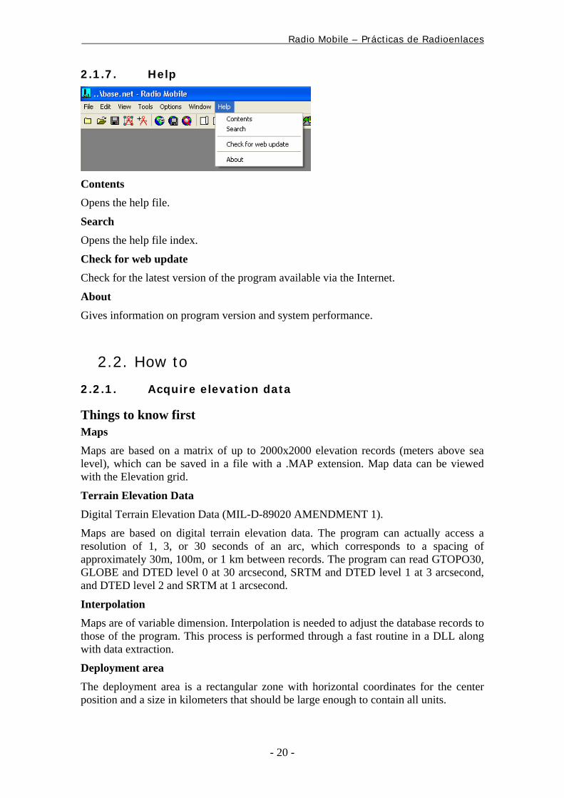
2.1.7. Help
Contents Opens the help file.
Search Opens the help file index.
Check for web update Check for the latest version of the program available via the Internet.
About Gives information on program version and system performance.
2.2. How to
2.2.1. Acquire elevation data
Things to know first Maps Maps are based on a matrix of up to 2000x2000 elevation records (meters above sea level), which can be saved in a file with a .MAP extension. Map data can be viewed with the Elevation grid.
Terrain Elevation Data Digital Terrain Elevation Data (MIL-D-89020 AMENDMENT 1).
Maps are based on digital terrain elevation data. The program can actually access a resolution of 1, 3, or 30 seconds of an arc, which corresponds to a spacing of approximately 30m, 100m, or 1 km between records. The program can read GTOPO30, GLOBE and DTED level 0 at 30 arcsecond, SRTM and DTED level 1 at 3 arcsecond, and DTED level 2 and SRTM at 1 arcsecond.
Interpolation Maps are of variable dimension. Interpolation is needed to adjust the database records to those of the program. This process is performed through a fast routine in a DLL along with data extraction.
Deployment area The deployment area is a rectangular zone with horizontal coordinates for the center position and a size in kilometers that should be large enough to contain all units.
Radio Mobile – Prácticas de Radioenlaces
- 21 -
Step by step 1. In View menu, select World map. On the world map picture, click on the desired position for the map center position.
2. In File menu, select Map properties. This will open a form with all the necessary controls to create a map. Click on Use cursor position button.
3. Optionally use city or DMS (Latitude and longitude in degree, minute, second) to enter a more precise position for the center of the map.
4. Select the database and associated database path. If you do not have a database, you can set SRTM parameters in Internet Preferences in Options in order to download elevation data directly from the Internet.
5. Select 400x400 pixels and 100 km size.
6. Click on the Apply button.
7. If an error message occurs, verify the database drive and redo from step 2.
8. In File menu, select New picture (See How to create a map picture).
2.2.2. Create a map picture
Things to know first Picture size Picture size is equal to the elevation matrix pixel size defined in Map properties. It has a direct impact on program performance. The amount of calculation increases by the square of picture side, as well as the memory needed. First try small pictures (400x400) to test your machine.
Video settings The best compromise is definitively 16-bit color setting (65536 colors). Some function gives poor results at 8 bits color setting (256 colors). More colors such as 24 bits kills memory.
Draw mode
Each mode can be used to enhance terrain characteristics. The most common draw mode is Gray scaled slope, because networks features are better seen.
About Picture properties Gray scaled slope This option is used to draw the topographic map using a gray color scale according to the terrain slope. In this mode, the map is drawn as if lighted from the azimuth entered in the Light Azimuth entry box, such that slopes facing the direction of the light source are the lightest, and slopes facing away from the light source are darker. Horizontal terrain is drawn with the average color shade given by the Brightness entry box. The range from lightest to darkest shade is prescribed by means of the Contrast entry box.
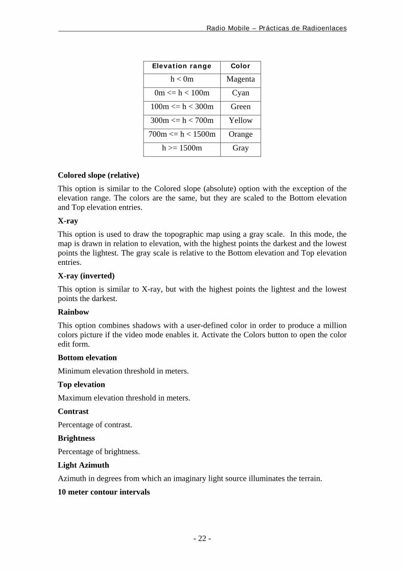
Colored slope (absolute)
This option is similar to the Gray scaled slope option with the exception of the color. In this mode, the color is related to the elevation (h) above sea level according to the following scale:
Radio Mobile – Prácticas de Radioenlaces
- 22 -
Elevation range Color
h < 0m Magenta
0m <= h < 100m Cyan
100m <= h < 300m Green
300m <= h < 700m Yellow
700m <= h < 1500m Orange
h >= 1500m Gray
Colored slope (relative) This option is similar to the Colored slope (absolute) option with the exception of the elevation range. The colors are the same, but they are scaled to the Bottom elevation and Top elevation entries.
X-ray This option is used to draw the topographic map using a gray scale. In this mode, the map is drawn in relation to elevation, with the highest points the darkest and the lowest points the lightest. The gray scale is relative to the Bottom elevation and Top elevation entries.
X-ray (inverted) This option is similar to X-ray, but with the highest points the lightest and the lowest points the darkest.
Rainbow This option combines shadows with a user-defined color in order to produce a million colors picture if the video mode enables it. Activate the Colors button to open the color edit form.
Bottom elevation Minimum elevation threshold in meters.
Top elevation Maximum elevation threshold in meters.
Contrast Percentage of contrast.
Brightness Percentage of brightness.
Light Azimuth Azimuth in degrees from which an imaginary light source illuminates the terrain.
10 meter contour intervals
Radio Mobile – Prácticas de Radioenlaces
- 23 -
This option generates darker contour curves at every 10m of elevation.
100 meter contour intervals This option generates darker contour curves at every 100m of elevation.
500 meter contour intervals This option generates darker contour curves at every 500m of elevation.
Draw objects This option will exhibit roads, lakes, boundaries and labels defined in .plt files (OziExplorer format) located in a sub directory object if they are within the map limits.
Show cities This option will exhibit cities defined in file cities.dat if they are within the map limits. If selected, font and back style can be selected with the Font button and Transparent checkbox.
Step-by-step 1. In File menu, select New picture.
2. Select Grey scaled slope, 30% contrast, 70% brightness, 335 deg. Light azimuth, no Cities, and no Contours.
3. Click on the Apply button.
2.2.3. Position units
Things to know first Cursor The cursor has a horizontal position with an elevation record (in meter above sea level) corresponding to intersection of the two dotted lines that appear after a click on the map. The Elevation grid (when selected in View menu) shows a 5x5 array of elevations surrounding the horizontal position that is shown in latitude/longitude coordinates, just below the Elevation grid. To move the cursor, click anywhere on a map picture or click on any cell of the Elevation grid.
Elevation Units automatically get an elevation (in meters above sea level) from the map when you position them. You can also enter the exact elevation manually if you know it.
Enabled This property determines if the unit is active and visible. It is useful to temporarily remove a unit without erasing the associated data.
Transparent
This option determines if the label uses the backcolor or if it is transparent.
Step by step 1. Click alternatively on the map picture and on the cells of the Elevation grid to localize the pixel where you want to position the unit.
Radio Mobile – Prácticas de Radioenlaces
- 24 -
2. In File menu select Unit properties. This will open a form with all the necessary controls to finalize the positioning of the unit.
3. Select a unit in the list.
4. Use the Name text box to edit the unit name. Click on the Place unit at cursor position button to force the entry of the cursor coordinates and elevation into the unit fields.
5. Set the visible, forecolor, transparent, and backcolor properties. Observe the changes with the example shown.
6. Close the Units properties form. The unit label should appear on the map picture.
Tip for repositioning Position the cursor to the wanted position. Click on the unit label with the right button of the mouse. The program will ask you to confirm the move. Click the OK button and the unit will jump to the new position. Note that if you double click on a unit label, the Unit properties form will open with the selected unit ready to be edited.
2.2.4. Create a network
Things to know first ITS model The US Institute for Telecommunications Science (ITS) has published a well-known model for radio propagation commonly referred to as the Longley-Rice model. The original code in FORTRAN has been translated into a dynamic link library for Windows. The input of the model includes environmental, system, and statistical parameters. The output is the predicted path loss between units.
Radio systems There are some technical parameters in addition to those of the ITS model that must be selected to compute the received signal knowing the path loss. The program supports 25 different configurations that are related to the radio installation in use.
Net topology The program does more than evaluate the quality of communication between units. If you have selected a network topology where rebroadcast is allowed, the program will initiate as much iteration as necessary to find the shortest successful path between units. If no path is found after the maximum number of rebroadcasts is reached, the link will be shown in red.
Net membership
Each unit entered in a net has a role and a radio system.
Net parameters Net name The net name can be up to 30 characters long.
Minimum and maximum frequency
Radio Mobile – Prácticas de Radioenlaces
- 25 -
For a frequency hopping net, these entries correspond to the lower and upper limits of the hopping set. The program computes the mean frequency as the entry for the propagation model.
Polarization Either horizontal or vertical (in accordance with the system in use).
Mode of variability The Spot mode is for a one-try message. The Accidental mode is for interference evaluation. The Mobile mode is for units that are moving while communicating. The Broadcast mode is for stationary units.
The effect of percentage of time, locations, and situations depends on the mode selected.
Surface refractivity The terrain surface refractivity is a measure of the air refractivity above/near the ground. In general, the average refractivity would decrease with altitude, being a maximum at sea level. In the absence of any specific data, the default value should be used.
Ground conductivity
Relative ground permittivity These properties determine together the nature of the radio wave reflection on the ground in a Line-Of-Sight radio link. In general, the more conductive the terrain is, the greater is the risk to have important attenuation or fluctuations of the radio signal. The worst case is the “picket fence” type. In the absence of any specific data, default values should be used.
Climate This option is used to select the type of climate mostly encountered in the selected deployment area.
Equatorial
Continental Subtropical
Maritime Sub-Tropical
Desert
Continental Temperate
Maritime Temperate Over Land
Maritime Temperate Over Sea
These options set some of the calculation parameters in the ITS algorithm used in the program. The atmospheric conditions like climate and weather vary in the different areas of the world, and affect both the refractive index of free air and play an important role in determining the strength and fading properties of radio signals. For instance, the refractive index gradient of air near the surface of the earth determines the way a radio ray is bent or refracted as it passes through the atmosphere.
The Continental Temperate climate is common to large landmasses in the Temperate Zone.
Cancel
Radio Mobile – Prácticas de Radioenlaces
- 26 -
Restores all net properties to their initial value, when the form was opened.
Default parameters Sets the propagation model parameters of a network to their defaults.
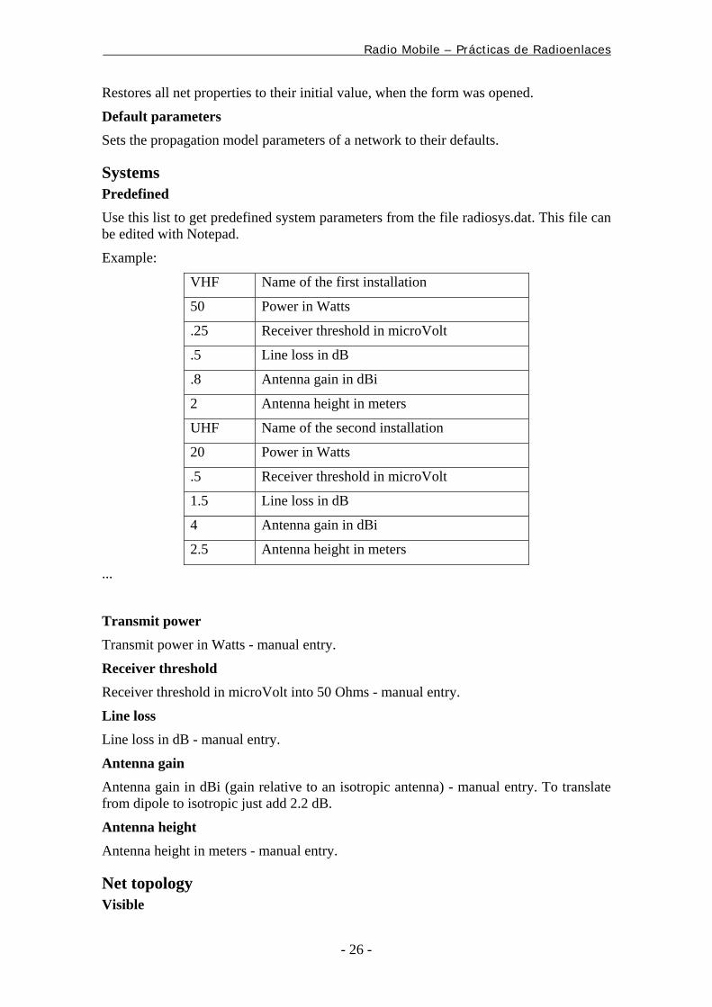
Systems Predefined Use this list to get predefined system parameters from the file radiosys.dat. This file can be edited with Notepad.
Example:
VHF Name of the first installation
50 Power in Watts
.25 Receiver threshold in microVolt
.5 Line loss in dB
.8 Antenna gain in dBi
2 Antenna height in meters
UHF Name of the second installation
20 Power in Watts
.5 Receiver threshold in microVolt
1.5 Line loss in dB
4 Antenna gain in dBi
2.5 Antenna height in meters
...
Transmit power Transmit power in Watts - manual entry.
Receiver threshold Receiver threshold in microVolt into 50 Ohms - manual entry.
Line loss Line loss in dB - manual entry.
Antenna gain
Antenna gain in dBi (gain relative to an isotropic antenna) - manual entry. To translate from dipole to isotropic just add 2.2 dB.
Antenna height Antenna height in meters - manual entry.
Net topology Visible
Radio Mobile – Prácticas de Radioenlaces
- 27 -
Use this check box to show or hide a net on the map picture.
Voice net Use this option for a net where needlines from command posts to subordinate units are required, but not between subordinates. Rebroadcast units can be used to increase the communication range.
Data net, star topology Use this option for a data net where a master unit polls slave units, with no links between slave units.
Data net, cluster Use this option for a data net with nodes that can retransmit datagrams (rebroadcast, digipeating).
Maximum number of rebroadcasts. If set to zero, this parameter will inhibit retransmission.
Otherwise: (Maximum number of rebroadcasts) = (Time to live) - 1
Net membership List of all units Use the checkbox at the left of the List of all units to add or remove units to the net. Select a role and a system for each unit with the lists on the right. To verify the role and the system that were already assigned to a unit, click the unit name in the List of all units.
Member role and system Since many units in a net may share some technical parameters, these parameters were regrouped under a same system definition to reduce memory usage. As soon as a unit has a parameter that differs from the other units, a new system must be defined for that unit. The only exception is the antenna height, which can be overwritten.
Style (Applies to all nets) Propagation mode Toggle between Normal or Interference propagation mode. For interference studies, the model is optimistic.
Network drawing colors User can select color and threshold for network drawing.
Step by step 1. In File menu select Networks properties.
2. Press the Net parameters button.
3. Use the List of all nets to select the network to be edited.
4. Edit the network name and all radio propagation parameters
5. Press the Net topology button.
Radio Mobile – Prácticas de Radioenlaces
- 28 -
6. Check Visible and select the Voice net topology.
7. Press the Systems button.
8. Use the List of all systems to edit as many systems as necessary to describe the network.
9. Press the Net membership button.
10. Check units to be in the network. For each unit select a role and a system.
2.2.5. Save and retrieve projects
Networks file (*.net) includes: Radio propagation parameters, topology, and membership for the 25 nets in memory
Technical data for the 25 radio systems in memory
Properties for the 50 units in memory
Map filename
Pictures filenames
Antenna height values for units whose differs from system entry.
Step by step 1.Save the elevation matrix first with Save map as
2. Save each individual picture with Save picture as
3. Save networks and unit data with Save networks as
4. In File menu, select New networks to clear all.
5. In File menu, select Open networks and select the previously saved file.
6. Verify that all data and pictures have been recovered.
2.2.6. Perform radio coverage
Things to know first Radio coverage of what? Suppose a unit is stationary while the other is moved everywhere around. The system parameters are the same as those seen in Radio link, except for the position of the mobile unit.
Performance to meet The program uses Rx Threshold in S-unit, in microVolt, dBm or in microVolt/m. The performance thresholds in S-unit are relative to receiver sensitivity while the others are taken at the receiver input (see Radio link and system performance).
Single Polar
The surface is covered according to polar coordinates around the center unit. Range and azimuth span, and azimuth increment can be adjusted.
Combined Cartesian
Radio Mobile – Prácticas de Radioenlaces
- 29 -
The surface is covered according to small squares of variable pixel size. Many sites can be used to produce a combined coverage with the best signal available at each position on the map.
Interference The surface is covered according to small squares of variable pixel size. The coverage of a single transmitter side can be shown in two colors: the first color shows the normal coverage according to a minimum signal to meet, while the second color indicates that a signal from a second transmitter is interfering. Interference occurs when the minimum Signal to Interference ratio is not met.
Rendering Fill area and/or signal contours can be selected. Coverage color is mixed to the map picture with a logical and. (Better resolution means more computer time).
Antenna pattern If a non-directional antenna is used for center unit, the antenna will be pointed toward the original right unit position. This orientation can be modified with the antenna azimuth text box.
Step by step 1. Create a gray slope picture map (see How to create a map picture)
2. Position the center unit (see How to position units)
3. Enter network parameters for the center unit and mobile unit (see How to create a network)
4. In the Tools menu select Radio coverage then Single Polar
5. Select appropriate center unit, mobile unit, and net.
6. Select Threshold of 1 and 11 S-unit, radial range from 0 to 100 km, azimuth range from 0 deg. to 360 deg. at 1 deg. step.
7. Check the Fill area with yellow color.
8. Click the Apply button.
2.2.7. Perform visual coverage
Things to know first Applicability Visual coverage can be used for line of sight, radar or interception range. It is based on pure geometrical clearance, taking into account the sensor height above ground, the target height above ground (nap of the earth flight), the topography, and the earth curvature.
Earth radius Visual coverage uses the average earth radius to simulate earth curvature. This explains the difference observed with the radio coverage, where the radio beam tends to bend toward ground.
Radio Mobile – Prácticas de Radioenlaces
- 30 -
Step by step 1. Create a gray slope picture map (see How to create a map picture)
2. Position the center unit (see How to position units)
3. In Tools menu select Visual coverage
4. Select appropriate center unit, sensor height and target height.
5. Set radial range from 0 to 100 km, azimuth range from 0 deg. to 360 deg. at 1 deg. step.
6. Press the Yellow button.
2.2.8. Create an ADRG picture
Things to know first ADRG
ARC (equal Arc second Raster Chart/map) Digitized Raster Graphics (MIL-A-89007). Digital representation of graphics products: Maps are converted into digital data by raster scanning and transforming the map image into the ARC System frame of reference.
ADRG Picture properties ADRG picture are oriented, sized and stretched to fit elevation matrix, so each pixel corresponds to an elevation record. ADRG rendering depends on the map size selected.
Step by step 1. Insert the appropriate ADRG CD-ROM that covers the area of interest.
2. In File menu, select Picture properties.
3. Press the ADRG button.
4. Change the ADRG CD-ROM if necessary to complete the picture when prompted.
2.2.9. Import and scale user pictures
Things to know first Valid source The program can load BMP, GIF or JPEG bitmaps of satellite photo, scanned maps, etc.
Calibration
A picture must be calibrated in order to use it for positioning by entering the four corners latitude and longitude.
Step by step 1. In File menu, select Open picture.
2. Select a picture that is not already a map picture
3. Active the picture window and in File menu, select Picture properties.
Radio Mobile – Prácticas de Radioenlaces
- 31 -
4. Enter the latitude and longitude of each of the corners (you can use the cursor position).
5. Press the Apply button.
2.2.10. Create a flight animation
Things to know first Flight path The flight follows a direct line from Tx antenna to Rx antenna.
Disk space The flight animation uses a huge amount of disk memory. It is wise to import all the bitmaps into video animation software capable of compression, such as GIF Constructor shareware.
Step by step 1. In Tools menu select Radio link
2. If a valid link is shown, go to View and then Observe.
3. Use Options to specify the number of frames per second and flight speed.
4. Select Create normal flight.
5. After completion, play the animation in real time with View flight or Flight in View
2.2.11. Export profile data
Things to know first Export file format The program can export profile data into a file in text format. This file can be viewed with Windows Notepad or imported into a spreadsheet program.
Rmpath program Rmpath is a simple freeware that can be used to look at the profile data exported by the program. If this program is in the application directory, it will open automatically after saving the file.
Step by step 1. In Tools menu select Radio link
2. If a valid link is shown, go to Edit and then Export to….
3. Open Windows Notepad to view the profile data.
Use a local GPS and report position
Things to know first GPS serial output Most GPS are capable of sending information through a simple serial link. Only the TXD and GROUND pins need to be connected to the PC, on any of the serial port. The GPS must be set at 4800 or 9600 bps, 8 bits, No Parity, and 1 stop bit.
Radio Mobile – Prácticas de Radioenlaces
- 32 -
GPS sentence recognized The program looks for a sentence beginning with $GPRMC from the GPS. This sentence is common to most GPS.
UDP protocol The program uses Multicast UDP protocol to report position to other PCs running the program. This protocol is common to most LAN and can be used on the Internet, as soon as the IP address (or domain name, or computer ID) and port are valid.
Step by step 1. In Options menu select GPS options
2. Enter the serial port at which the GPS is connected.
3. Enter unit to move. This is the unit that will move according to the GPS position received.
4. Enter IP address and port at which position will be reported.
5. Press Start to initiate local GPS decoding. Color dot on the Status Bar should flash to show activity.
6. If Log was checked, sentences will be saved on file. Use Play back to verify.
2.3. Basics
2.3.1. Radio propagation model
Introduction This software is a tool to help in the elaboration of radio communication networks. Before implementing a network in the field, it can be used to verify the performance of network radio links.
The computer program evaluates if a radio link is possible between two given sites, and provides the performance of that link taking into account:
a. The radio equipment characteristics,
b. The radio wave propagation theory (using the US Institute for Telecommunications Science (ITS) propagation prediction model, better known as the Longley-Rice model (Notes 1 and 2)).
Note 1 Georges A. Hufford, Anita G. Longley and William A. Kissick. A Guide to the Use of the ITS Irregular Terrain Model in the Area Prediction Mode, National Telecommunications and Information Administration (NTIA) Report 82-100, US Department of Commerce, April 1982.
Note 2 Anita G. Longley. Radio Propagation in Urban Area, Institute of Telecommunication Sciences, Office of Telecommunications, Boulder, Colorado 80302.
Radio Mobile – Prácticas de Radioenlaces
- 33 -
Suggested values for surface parameters Ground attribute Ground Conductivity Relative Permittivity
Average ground 005 15
Poor ground 001 4
Good ground .02 25
Fresh water .01 25
Sea water 5 25
2.3.2. Radio link and system performance
Radio link menu bar Edit Use Copy to send a copy of the active form picture to the clipboard.
Use Export to... to save profile data in a file and open the RMPATH program.
View Use Profile to initiate execution of the profile extraction and link performance calculation between the units selected in the left and right lists. Changing units in either list or changing the net (middle list) will initiate the same process. The left unit transmits toward the right unit.
Use Swap to exchange Tx and Rx units.
Use Details for a short performance report, such as distance, azimuth, mode of propagation, and system data.
Use Range to view the signal and distance relationship. The cursor is positioned at the distance where the signal does not meet the required performance (range).
Use Distribution to view the signal statistical distribution relative to receiver performance.
Use Observe and select either the 5°, 10°, 20°, 40° or 80° angle of view to visually observe the right unit as seen from the left unit.
Profile picture Clicking on the profile picture will move the receiver along the path. The label indicates the distance, clearance or obstruction, and signal. The 0.6F1 symbol means 0.6 times the first Fresnel zone.
S-meters Each of the green lights correspond to one S-unit, the red lights each correspond to an additional 10 dB over S9. The right S-meter corresponds to the signal received for a transmission from left to right. The left S-meter corresponds to the signal received for a transmission from the right to the left. The values may differ if the system gains are different in each case.
Radio link performance The performance of a radio link is calculated as per the following:
Radio Mobile – Prácticas de Radioenlaces
- 34 -
T (dBm) = 10 log10 (Transmit power in Watts) + 30
L1 (dB) = Transmitter line loss
A1 (dBi) = Transmitter antenna gain relative to an isotropic antenna
P (dB) = Radio propagation loss from the Longley-Rice model (including required fade margin)
A2 (dBi) = Receiver antenna gain relative to an isotropic antenna
L2 (dB) = Receiver line loss
R (dBm) = 20 log10 (Receiver threshold in microvolts) - 107
The performance shown in dB:
M (dB) = Received signal (dBm) - R (dBm)
M (dB) = (Tx - L1 + A1 - P + A2 - L2 ) - R
The performance shown in S-Units for frequencies < 30 MHz:
S0 (M <= -3dB)
S1 (M > -3dB and M <3dB)
S2 (M >= 3dB and M <= 9dB)
S3 (M > 9dB and M < 15dB)
S4 (M >= 15dB and M <= 21dB)
S5 (M > 21dB and M < 27dB)
S6 (M >= 27dB and M <= 33dB)
S7 (M > 33dB and M < 39dB)
S8 (M >= 39dB and M <= 45dB)
S9 (M > 45dB and M < 54dB)
S9 + 10 (M >= 54dB and M < 63dB)
S9 + 20 (M >= 63dB and M < 73dB)
S9 + 30 (M >= 73dB and M < 83dB)
The performance shown in S-Units for frequencies >= 30 MHz:
S0 (M <= -1.5dB)
S1 (M > -1.5dB and M <1.5dB)
S2 (M >= 1.5dB and M <= 4.5dB)
S3 (M > 4.5dB and M < 7.5dB)
S4 (M >= 7.5dB and M <= 10.5dB)
S5 (M > 10.5dB and M < 13.5dB)
S6 (M >= 13.5dB and M <= 16.5dB)
S7 (M > 16.5dB and M < 19.5dB)
S8 (M >= 19.5dB and M <= 22.5dB)
Radio Mobile – Prácticas de Radioenlaces
- 35 -
S9 (M > 22.5dB and M < 27dB)
S9 + 10 (M >= 27dB and M < 39dB)
S9 + 20 (M >= 39dB and M < 49dB)
S9 + 30 (M >= 49dB and M < 59dB)
2.3.3. 3D, panoramic, and stereoscopic views
3D picture The 3D picture is an option available in the Picture properties form. It uses a 2D-map picture as a source for pixel color, each pixel of the 2D picture corresponding to a polygon in the 3D picture. The polygons are filling the space between successive pixels, after a geometrical transformation. The angle of view can be set with the scroll bars in the 3D picture properties form. 3D picture can be used to show the networks as well: Networks elevation can be modified without having to redraw the picture by using the Show nets command.
Stereo The stereoscopic picture is also an option available in the Picture properties form. It uses a 2D-map picture as a source for pixel color. It covers the same area as the 2D picture, except that it uses color separation (Red and blue glasses required) to gives left and right eyes different point of view, which gives the impression that the picture is popping out of the screen. A special cursor can be moved with the keyboard arrows (horizontal coordinates) and the + or - keys (elevation).
Observation view The observation view is available after a successful profile extraction in the Radio link window. Angle of view can be adjusted to zoom into the picture. Observation is from Tx antenna to Rx antenna. White and black circles are drawn when the Rx antenna is visible.
Stereo view The stereoscopic observation is similar to the observation view, except that it uses color separation (Red and blue glasses required) to gives left and right eyes different point of view, which gives the impression that the picture is popping out of the screen. Stereoscopic effect can be exaggerated by increasing distance between eyes in Options.
2.3.4. Geodesic, UTM, and MGRS coordinates
WGS The World Geodetic System (WGS) is used to set the horizontal position of a unit. In the program, Latitude ranges from 90° South to 90° North, and Longitude ranges from 180° West to 180° east.
UTM Universal Transverse Mercator (UTM) divides earth into 60 zones of 6 degrees of longitude. The Northing is the distance from the equator (m) while the Easting is the distance from the central longitude of the zone (m), added with 500 000.
Radio Mobile – Prácticas de Radioenlaces
- 36 -
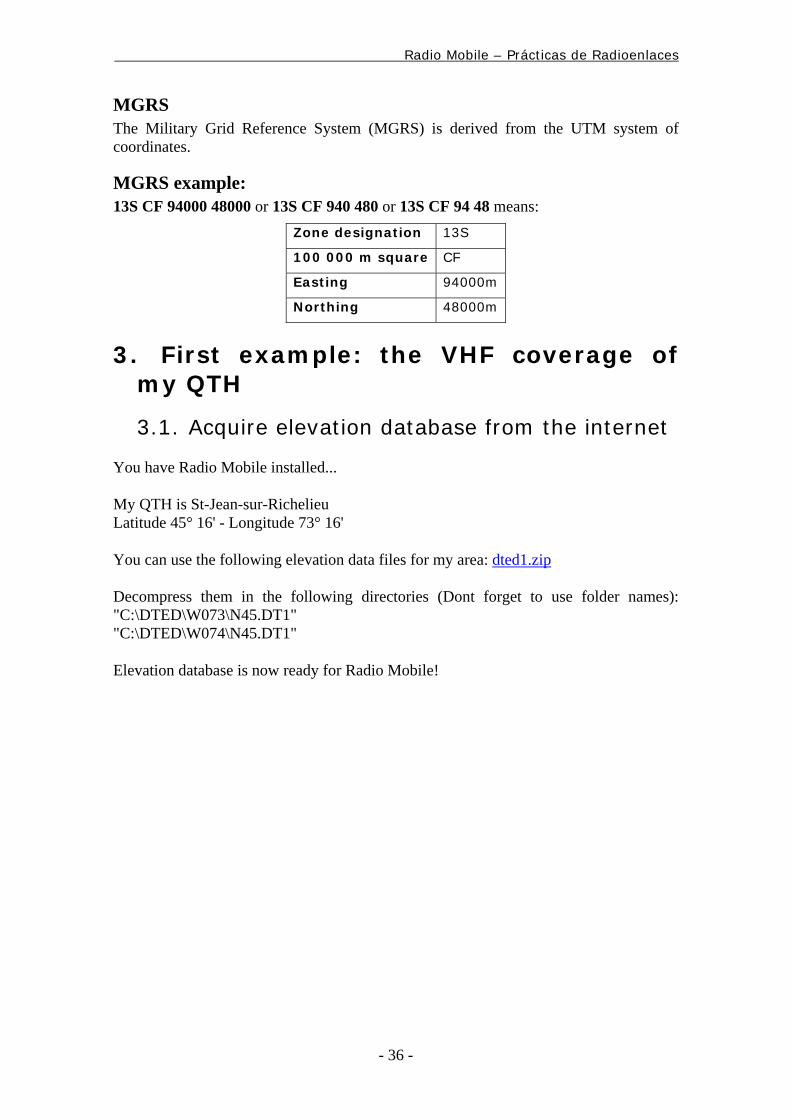
MGRS The Military Grid Reference System (MGRS) is derived from the UTM system of coordinates.
MGRS example: 13S CF 94000 48000 or 13S CF 940 480 or 13S CF 94 48 means:
Zone designation 13S
100 000 m square CF
Easting 94000m
Northing 48000m
3. First example: the VHF coverage of my QTH
3.1. Acquire elevation database from the internet
You have Radio Mobile installed...
My QTH is St-Jean-sur-Richelieu Latitude 45° 16' - Longitude 73° 16'
You can use the following elevation data files for my area: dted1.zip
Decompress them in the following directories (Dont forget to use folder names): "C:\DTED\W073\N45.DT1" "C:\DTED\W074\N45.DT1"
Elevation database is now ready for Radio Mobile!
Radio Mobile – Prácticas de Radioenlaces
- 37 -
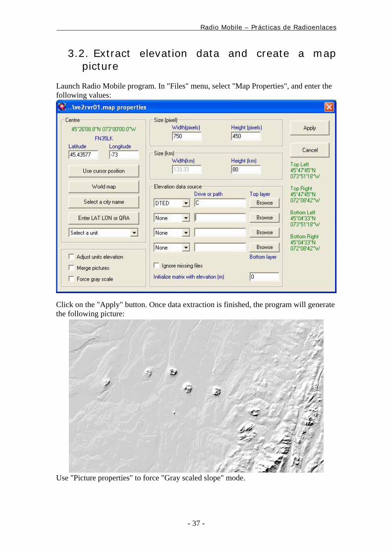
3.2. Extract elevation data and create a map picture
Launch Radio Mobile program. In "Files" menu, select "Map Properties", and enter the following values:
Click on the "Apply" button. Once data extraction is finished, the program will generate the following picture:
Use "Picture properties" to force "Gray scaled slope" mode.
Radio Mobile – Prácticas de Radioenlaces
- 38 -
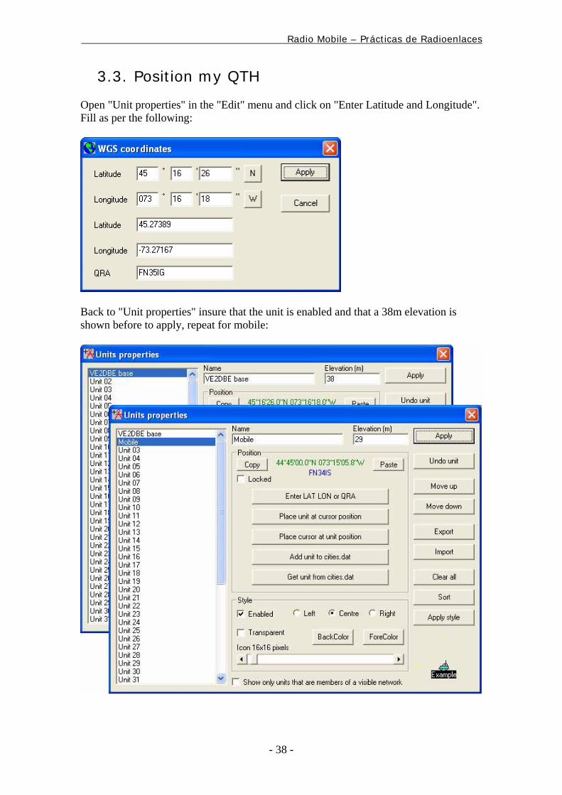
3.3. Position my QTH
Open "Unit properties" in the "Edit" menu and click on "Enter Latitude and Longitude". Fill as per the following:
Back to "Unit properties" insure that the unit is enabled and that a 38m elevation is shown before to apply, repeat for mobile:
Radio Mobile – Prácticas de Radioenlaces
- 39 -
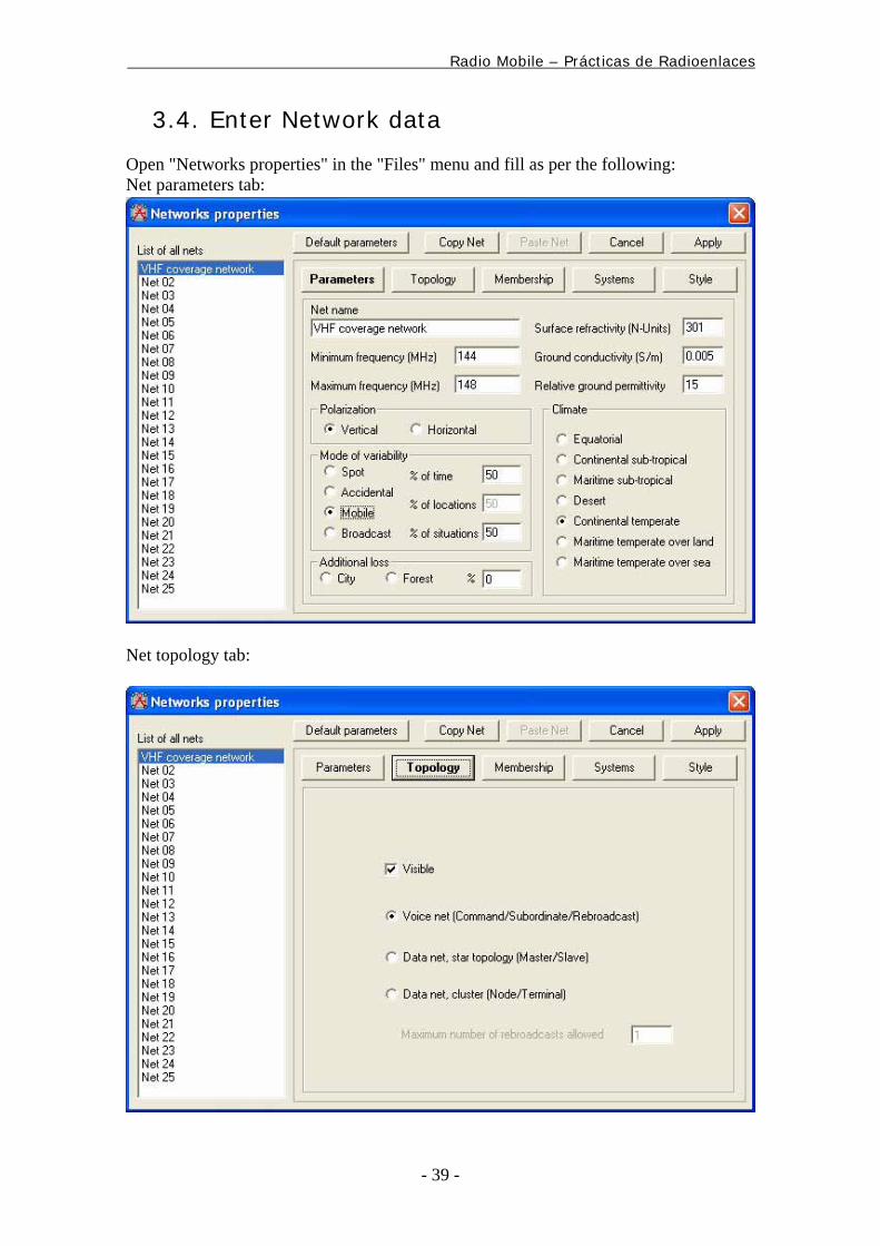
3.4. Enter Network data
Open "Networks properties" in the "Files" menu and fill as per the following: Net parameters tab:
Net topology tab:
Radio Mobile – Prácticas de Radioenlaces
- 40 -
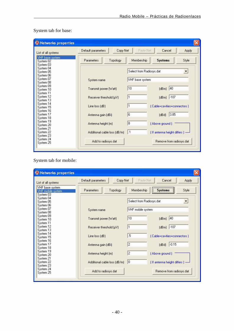
System tab for base:
System tab for mobile:
Radio Mobile – Prácticas de Radioenlaces
- 41 -
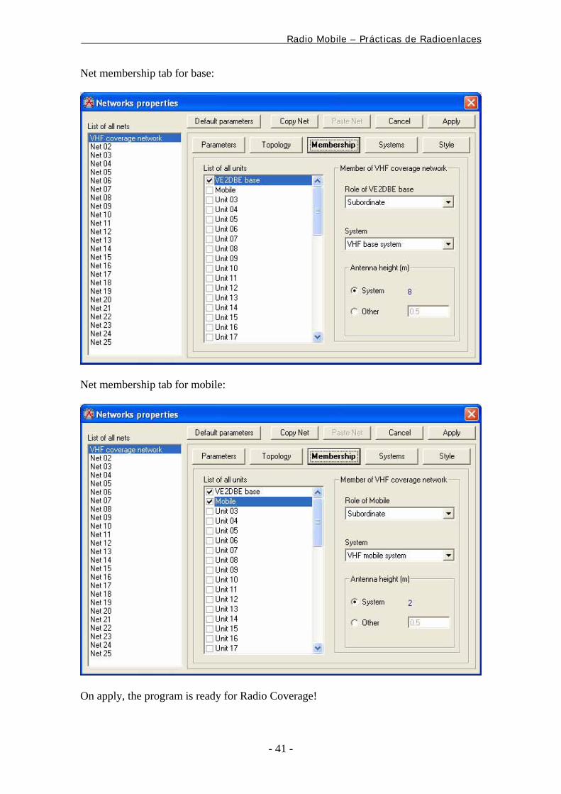
Net membership tab for base:
Net membership tab for mobile:
On apply, the program is ready for Radio Coverage!
Radio Mobile – Prácticas de Radioenlaces
- 42 -
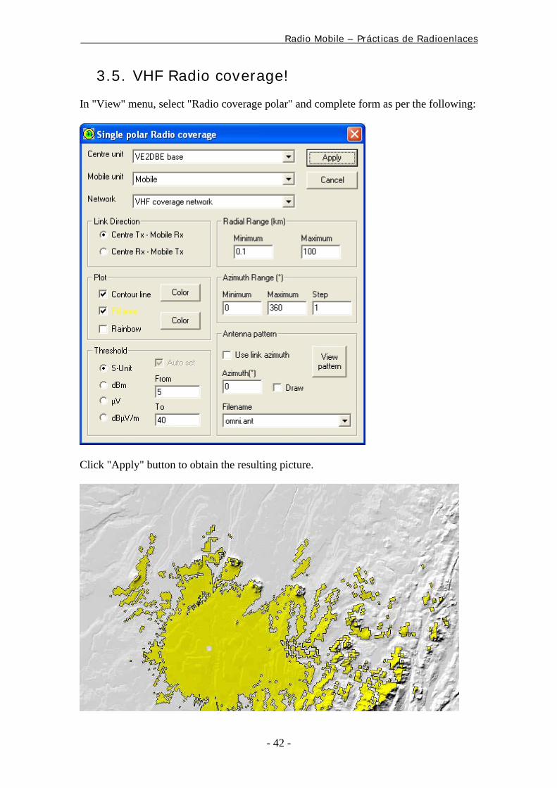
3.5. VHF Radio coverage!
In "View" menu, select "Radio coverage polar" and complete form as per the following:
Click "Apply" button to obtain the resulting picture.
Radio Mobile – Prácticas de Radioenlaces
- 43 -
4. Example 2: Introduction I found that when introducing my friends to Radio Mobile, that they had difficulty in setting up their first map and network to obtain an initial working display. The following is a description of a simple network setup, complete with a complimentary set of zipped files (which includes the required height - SRTM - data) to produce this network. For those of you who don't believe that Ashbourne is the centre of the world, you can enter your own Latitude and Longitude data in the 'Map Properties' window to give your local map after producing the working 'Base' network, with the program downloading your new SRTM data from the Internet as required. See the Notes section below for extra information and hints on some shortcuts.
I have also produced a second page 'Once you get going' which shows how extra units can be generated, some of the facilities available from the Radio Link window, and how to perform a Radio Coverage Plot. These two pages are available in .pdf format (1.3Mb) here.
More information at::
http://www.cplus.org/rmw/english1.html
http://www.g3tvu.co.uk/Quick%20Start.htm
There are a number of concepts which need to be understood when setting up and running the program. A radio station is referred to as a Unit, there can be numerous Units defined to operate within a given Network. Each different type of station used in a network has to be defined with a separate Radio System which sets the parameters for that type of station, i.e. Transmit Power/receiver sensitivity/antenna gain/antenna height/cable losses. Thus each Unit will be allocated to an operating system within the network. Finally, all units are given a Role, which is either Command or Subordinate. The effect of this is to set which links are shown on the network display - in my case, base is command so links are shown between command and the subordinate stations. Links between other pairs of stations can still be evaluated via the 'Radio Link' window.
4.1. Program setup
First download Visual Basic Runtime (Service Pack 6) from Microsoft (V86.0-KB290887-X86.exe) from:
http://www.microsoft.com/downloads/details.aspx?familyid=7B9BA261-7A9C-43E7-9117-F673077FFB3C&displaylang=es (for Spanish Windows versions)
http://www.microsoft.com/downloads/details.aspx?familyid=7B9BA261-7A9C-43E7-9117-F673077FFB3C&displaylang=es (for English Windows versions)
This has to be installed first on your machine by a double click on the file name after downloading, before any other files are installed. This may require a system reboot after installation, but the file can then be removed.
Then, generate a folder to hold your Radio Mobile files as in Roger's 'Download' web:
http://www.cplus.org/rmw/download.html
and 'How To' tutorials and pages:
http://www.cplus.org/rmw/howto.html
Radio Mobile – Prácticas de Radioenlaces
- 44 -
(I have used 'C:\Program Files\Radio Mobile' as base folder for my system as suggested).
To extract zipped files, Winzip available @ www.winzip.com, will be required, (although Internet Explorer 6 under XP does have an extraction Wizard).
4.2. Download my Zip file.
My Zip file (3.6Mb) contains all the data required for the 'Base' Network and Roger's system files, this should be downloaded and extracted into your own Radio Mobile folder. The height data is contained in the file named 'N53W002.hgt', which will be placed in a new folder called 'SRTM' in your Radio Mobile folder . This SRTM folder will be used to hold all additional download data for your area later - in my case located at 'C:\Program Files\Radio Mobile\SRTM'. Ensure that no other instances of rmwdlx32.dll exists on your system. If you want to put the program at more than one location, you should put rmwdlx32.dll in C:\Windows\System (C:\Winnt\System32 for NT). These files are correct at 5th Feb 2005 with version 6.3.0, updates can be download directly from the Download page.
My Quick Start Zip file is available here.
http://www.g3tvu.co.uk/Quick%20Start%20Files.zip
4.3. Setting up RMW.
After extracting the files, a shortcut for 'Radio Mobile' will be found in your 'Radio Mobile' folder and can be moved onto your desktop by 'left click and drag'. Open the program with a 'double click' on this shortcut (or on RMWDLX.exe), and the Radio Mobile window will open showing a 'Default' network (title \default.net). You will have to navigate to your Elevation data path, using the window below, to set up where internet data will be placed.
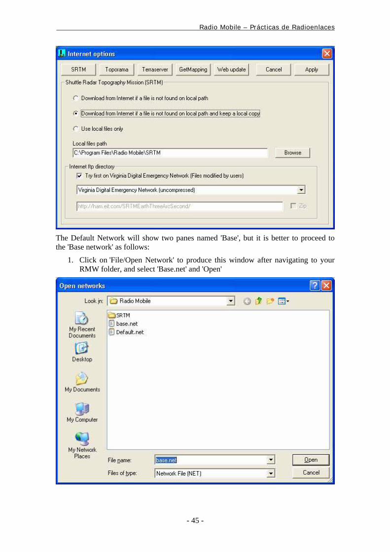
To set up the Elevation Data path, Click on 'Options/Internet' to produce this window, and browse to your local SRTM folder again as above, - click Apply.
Radio Mobile – Prácticas de Radioenlaces
- 45 -
The Default Network will show two panes named 'Base', but it is better to proceed to the 'Base network' as follows:
1. Click on 'File/Open Network' to produce this window after navigating to your RMW folder, and select 'Base.net' and 'Open'
Radio Mobile – Prácticas de Radioenlaces
- 46 -
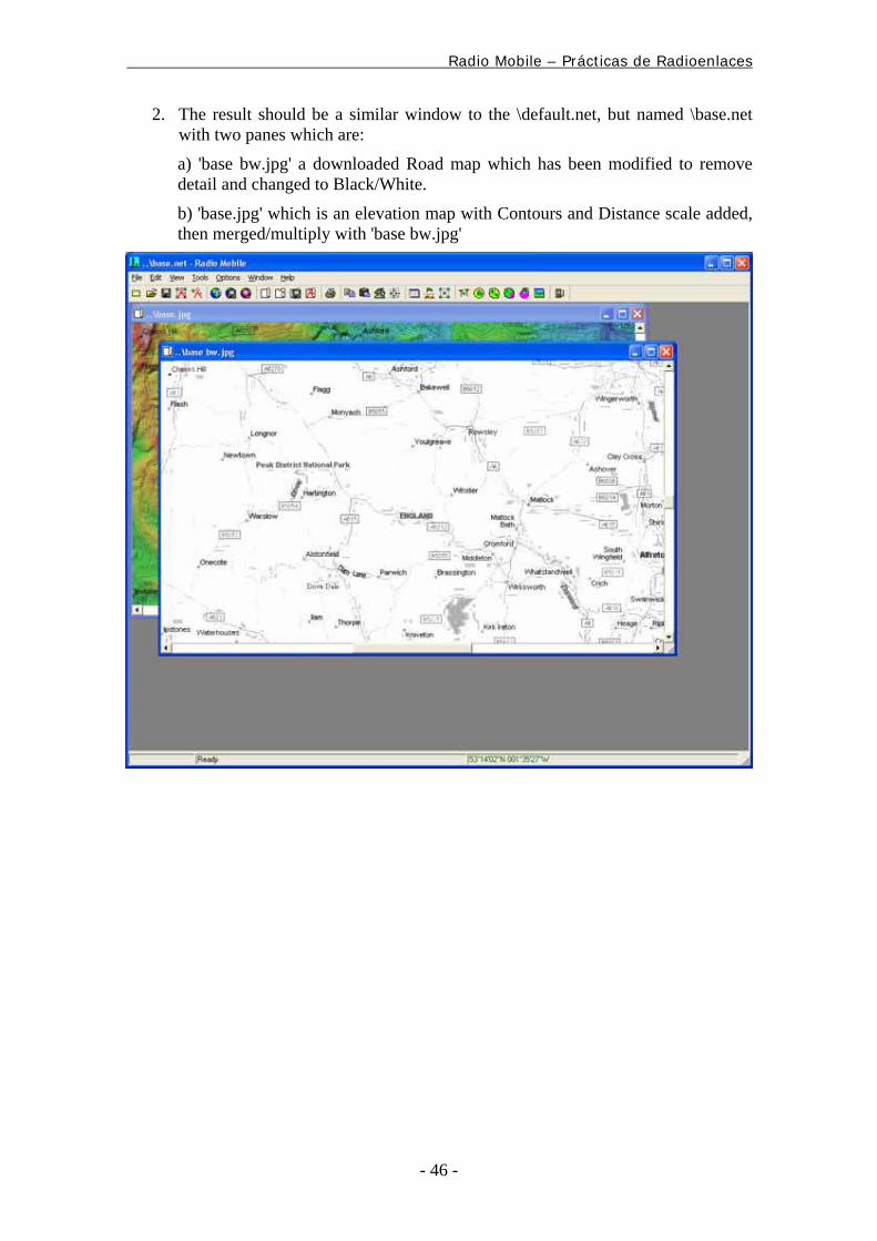
2. The result should be a similar window to the \default.net, but named \base.net with two panes which are:
a) 'base bw.jpg' a downloaded Road map which has been modified to remove detail and changed to Black/White.
b) 'base.jpg' which is an elevation map with Contours and Distance scale added, then merged/multiply with 'base bw.jpg'
Radio Mobile – Prácticas de Radioenlaces
- 47 -
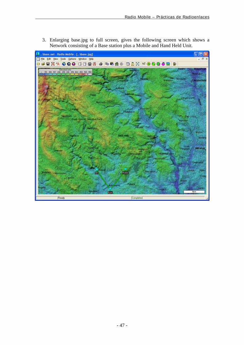
3. Enlarging base.jpg to full screen, gives the following screen which shows a Network consisting of a Base station plus a Mobile and Hand Held Unit.
Radio Mobile – Prácticas de Radioenlaces
- 48 -
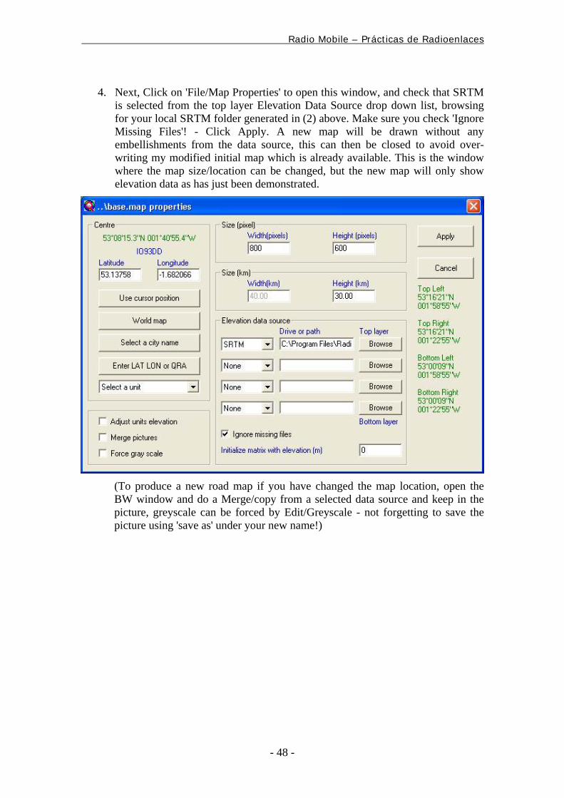
4. Next, Click on 'File/Map Properties' to open this window, and check that SRTM is selected from the top layer Elevation Data Source drop down list, browsing for your local SRTM folder generated in (2) above. Make sure you check 'Ignore Missing Files'! - Click Apply. A new map will be drawn without any embellishments from the data source, this can then be closed to avoid over-writing my modified initial map which is already available. This is the window where the map size/location can be changed, but the new map will only show elevation data as has just been demonstrated.
(To produce a new road map if you have changed the map location, open the BW window and do a Merge/copy from a selected data source and keep in the picture, greyscale can be forced by Edit/Greyscale - not forgetting to save the picture using 'save as' under your new name!)
Radio Mobile – Prácticas de Radioenlaces
- 49 -
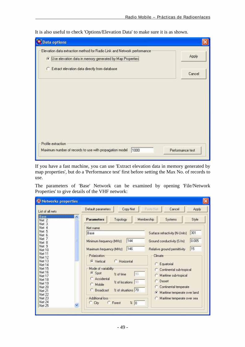
It is also useful to check 'Options/Elevation Data' to make sure it is as shown.
If you have a fast machine, you can use 'Extract elevation data in memory generated by map properties', but do a 'Performance test' first before setting the Max No. of records to use.
The parameters of 'Base' Network can be examined by opening 'File/Network Properties' to give details of the VHF network:
Radio Mobile – Prácticas de Radioenlaces
- 50 -
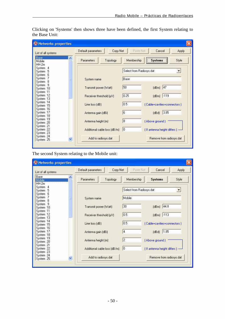
Clicking on 'Systems' then shows three have been defined, the first System relating to the Base Unit:
The second System relating to the Mobile unit:
Radio Mobile – Prácticas de Radioenlaces
- 51 -
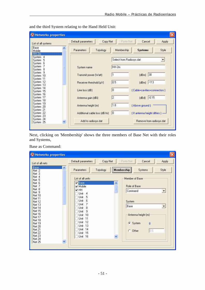
and the third System relating to the Hand Held Unit:
Next, clicking on 'Membership' shows the three members of Base Net with their roles and Systems,
Base as Command:
Radio Mobile – Prácticas de Radioenlaces
- 52 -
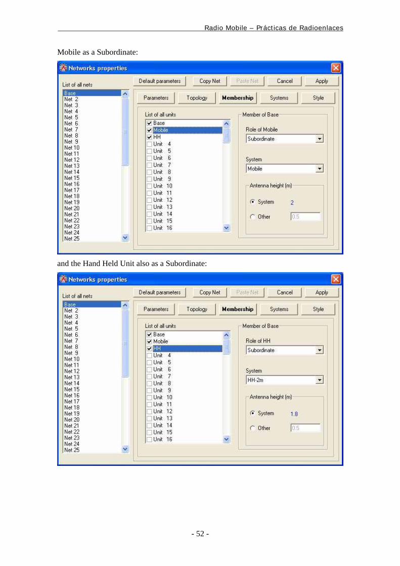
Mobile as a Subordinate:
and the Hand Held Unit also as a Subordinate:
Radio Mobile – Prácticas de Radioenlaces
- 53 -
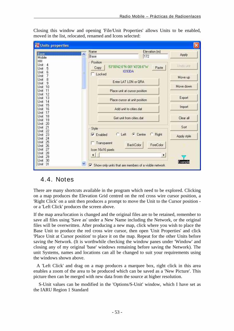
Closing this window and opening 'File/Unit Properties' allows Units to be enabled, moved in the list, relocated, renamed and Icons selected:
4.4. Notes
There are many shortcuts available in the program which need to be explored. Clicking on a map produces the Elevation Grid centred on the red cross wire cursor position, a 'Right Click' on a unit then produces a prompt to move the Unit to the Cursor position - or a 'Left Click' produces the screen above.
If the map area/location is changed and the original files are to be retained, remember to save all files using 'Save as' under a New Name including the Network, or the original files will be overwritten. After producing a new map, click where you wish to place the Base Unit to produce the red cross wire cursor, then open 'Unit Properties' and click 'Place Unit at Cursor position' to place it on the map. Repeat for the other Units before saving the Network. (It is worthwhile checking the window panes under 'Window' and closing any of my original 'base' windows remaining before saving the Network). The unit Systems, names and locations can all be changed to suit your requirements using the windows shown above.
A 'Left Click' and drag on a map produces a marquee box, right click in this area enables a zoom of the area to be produced which can be saved as a 'New Picture'. This picture then can be merged with new data from the source at higher resolution.
S-Unit values can be modified in the 'Options/S-Unit' window, which I have set as the IARU Region 1 Standard
Radio Mobile – Prácticas de Radioenlaces
- 54 -
This Network was produced at 800x600 pixels to reduce file sizes, similarly the pictures are saved in .jpg format. The reason for my Base Station being at the bottom of my map is to have all the units in one SRTM tile - where I live requires four tiles for the Base to be centralised! Map Properties can be changed to suit, with a size up to 2000 pixels square, and Lat/Long changed for your location. The Black and White road map is a very useful tool for coverage and Field Strength plots, as rainbow elevation colours - or sometimes greyscale - can obscure the colour changes.
Additional folders for DTED and other data can be produced in the Radio Mobile folder, then navigated to via the 'Internet Options' window.
Extracting the 'Quick Start' files into a folder 'C:\Program Files\Radio Mobile' ought to produce a working network with all the settings set as the above windows (other than the Elevation data paths) - this has been tried successfully on another new computer, so I hope it works on yours!
Radio Mobile – Prácticas de Radioenlaces
- 55 -
5. Advanced Guide Once you have managed to generate a working 'Base Network', there are a great number of facilities available to you within the program which can be explored. This is a starting point with Creating and adding extra Units, the Radio Link window, and a Radio Coverage plot.
5.1. Creating Extra Units
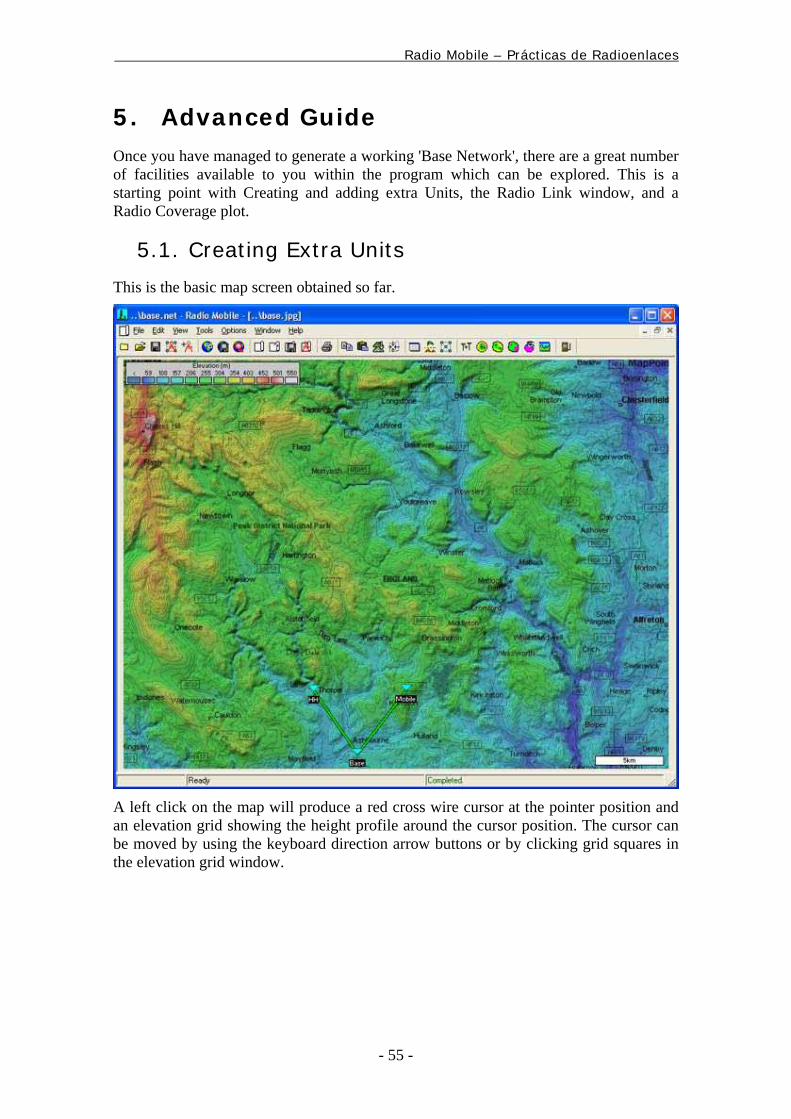
This is the basic map screen obtained so far.
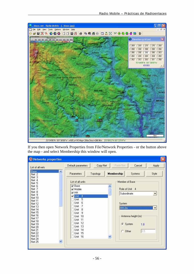
A left click on the map will produce a red cross wire cursor at the pointer position and an elevation grid showing the height profile around the cursor position. The cursor can be moved by using the keyboard direction arrow buttons or by clicking grid squares in the elevation grid window.
Radio Mobile – Prácticas de Radioenlaces
- 56 -
If you then open Network Properties from File/Network Properties - or the button above the map - and select Membership this window will open.
Radio Mobile – Prácticas de Radioenlaces
- 57 -
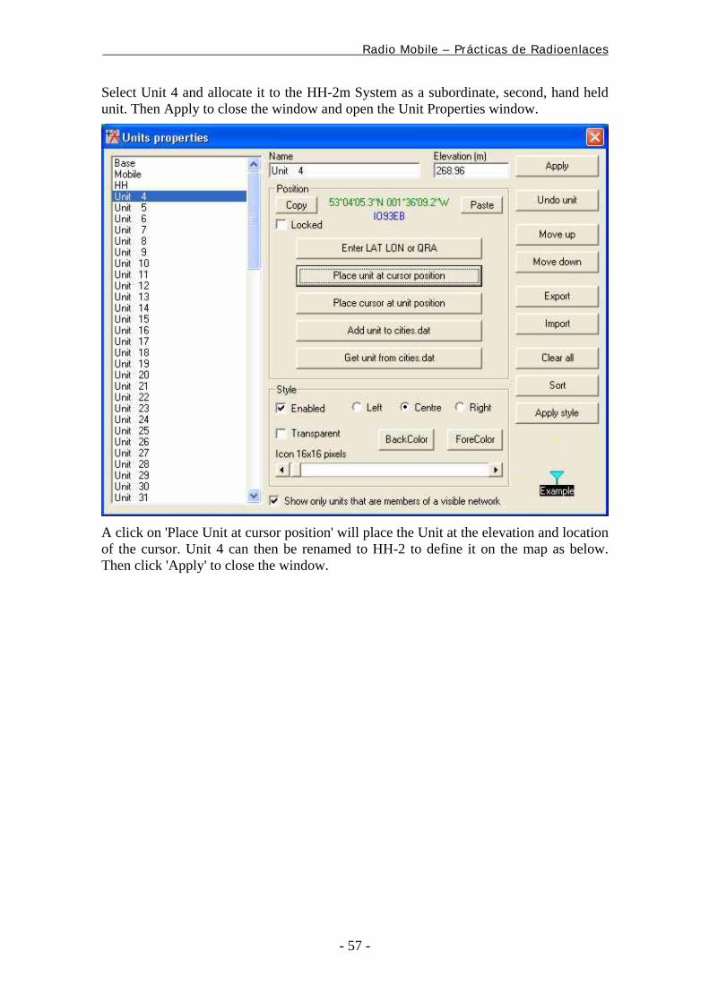
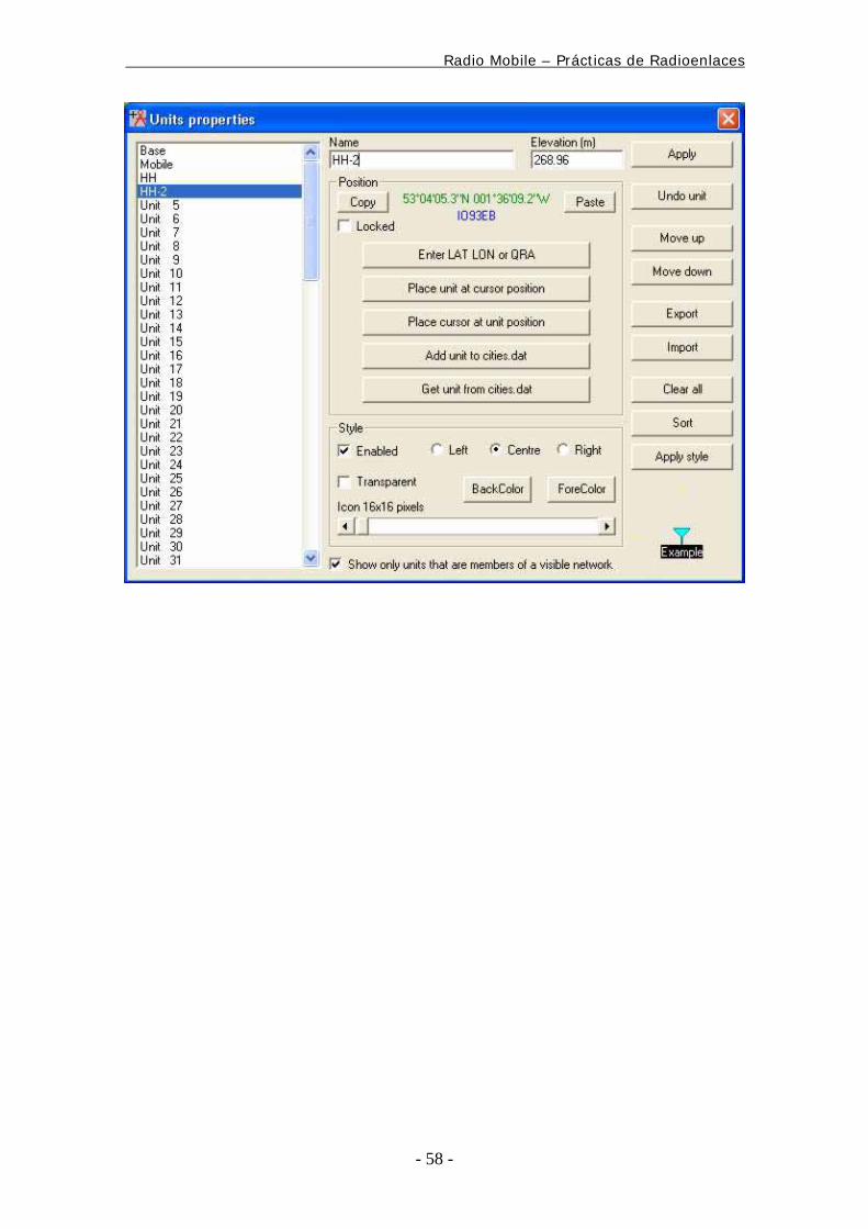
Select Unit 4 and allocate it to the HH-2m System as a subordinate, second, hand held unit. Then Apply to close the window and open the Unit Properties window.
A click on 'Place Unit at cursor position' will place the Unit at the elevation and location of the cursor. Unit 4 can then be renamed to HH-2 to define it on the map as below. Then click 'Apply' to close the window.
Radio Mobile – Prácticas de Radioenlaces
- 58 -
Radio Mobile – Prácticas de Radioenlaces
- 59 -
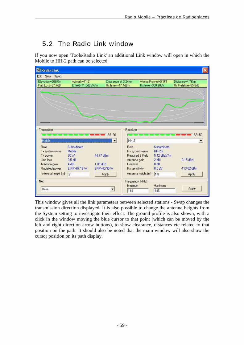
5.2. The Radio Link window
If you now open 'Tools/Radio Link' an additional Link window will open in which the Mobile to HH-2 path can be selected.
This window gives all the link parameters between selected stations - Swap changes the transmission direction displayed. It is also possible to change the antenna heights from the System setting to investigate their effect. The ground profile is also shown, with a click in the window moving the blue cursor to that point (which can be moved by the left and right direction arrow buttons), to show clearance, distances etc related to that position on the path. It should also be noted that the main window will also show the cursor position on its path display.
Radio Mobile – Prácticas de Radioenlaces
- 60 -
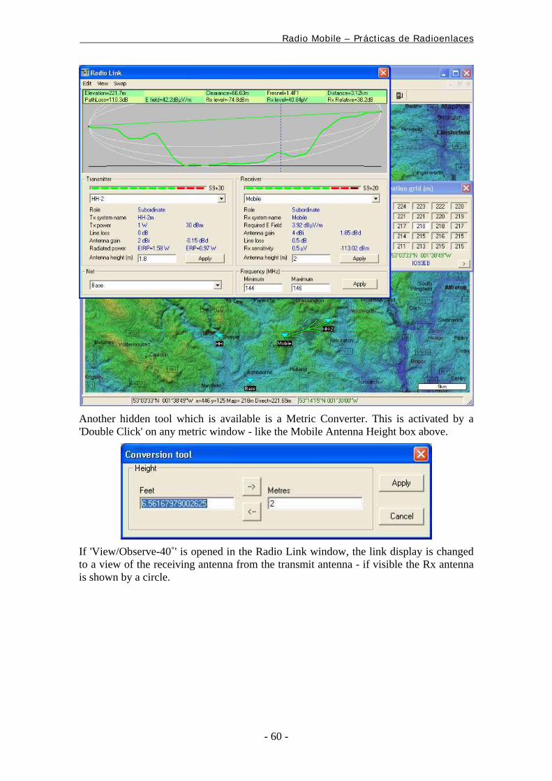
Another hidden tool which is available is a Metric Converter. This is activated by a 'Double Click' on any metric window - like the Mobile Antenna Height box above.
If 'View/Observe-40˚' is opened in the Radio Link window, the link display is changed to a view of the receiving antenna from the transmit antenna - if visible the Rx antenna is shown by a circle.
Radio Mobile – Prácticas de Radioenlaces
- 61 -
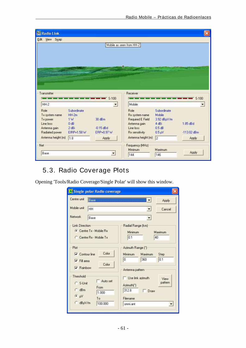
5.3. Radio Coverage Plots
Opening 'Tools/Radio Coverage/Single Polar' will show this window.
Radio Mobile – Prácticas de Radioenlaces
- 62 -
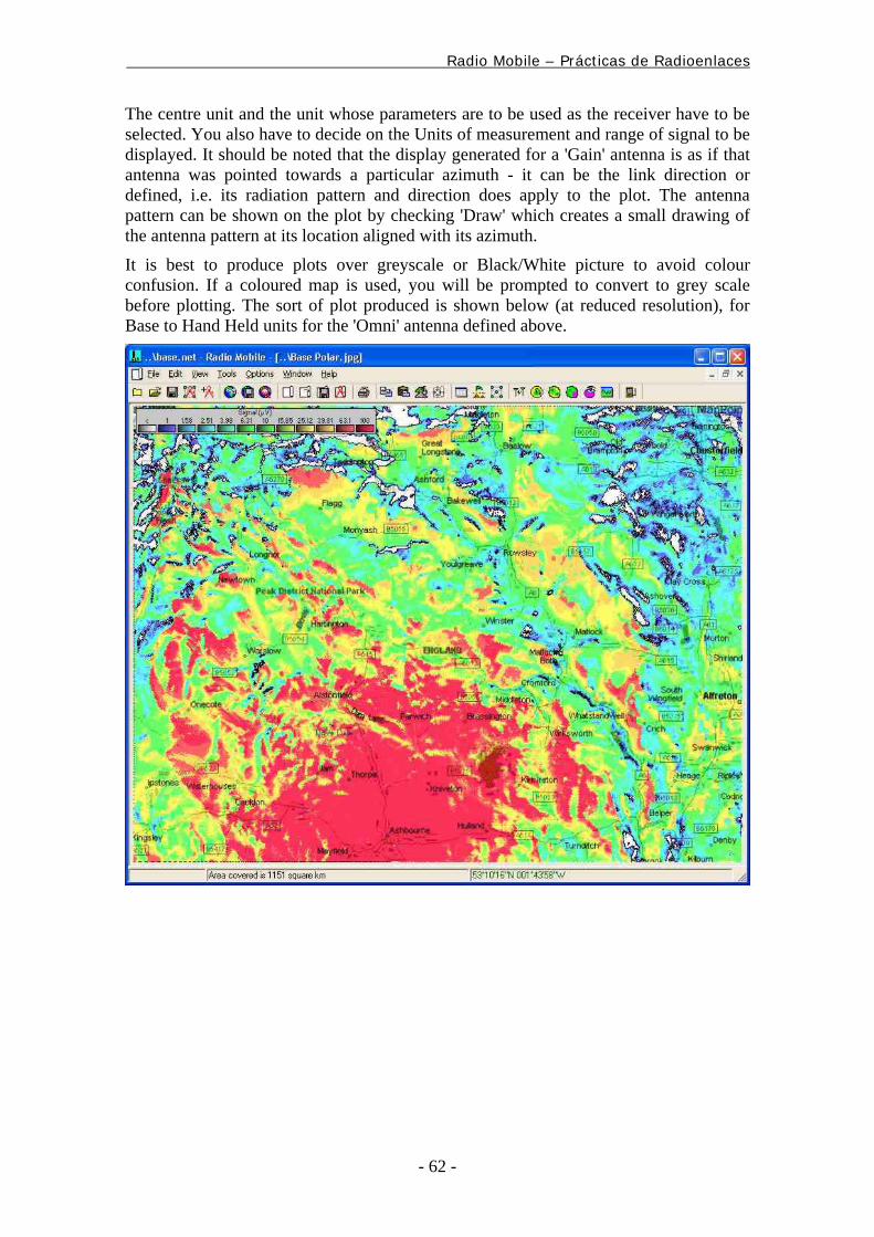
The centre unit and the unit whose parameters are to be used as the receiver have to be selected. You also have to decide on the Units of measurement and range of signal to be displayed. It should be noted that the display generated for a 'Gain' antenna is as if that antenna was pointed towards a particular azimuth - it can be the link direction or defined, i.e. its radiation pattern and direction does apply to the plot. The antenna pattern can be shown on the plot by checking 'Draw' which creates a small drawing of the antenna pattern at its location aligned with its azimuth.
It is best to produce plots over greyscale or Black/White picture to avoid colour confusion. If a coloured map is used, you will be prompted to convert to grey scale before plotting. The sort of plot produced is shown below (at reduced resolution), for Base to Hand Held units for the 'Omni' antenna defined above.
Radio Mobile – Prácticas de Radioenlaces
- 63 -
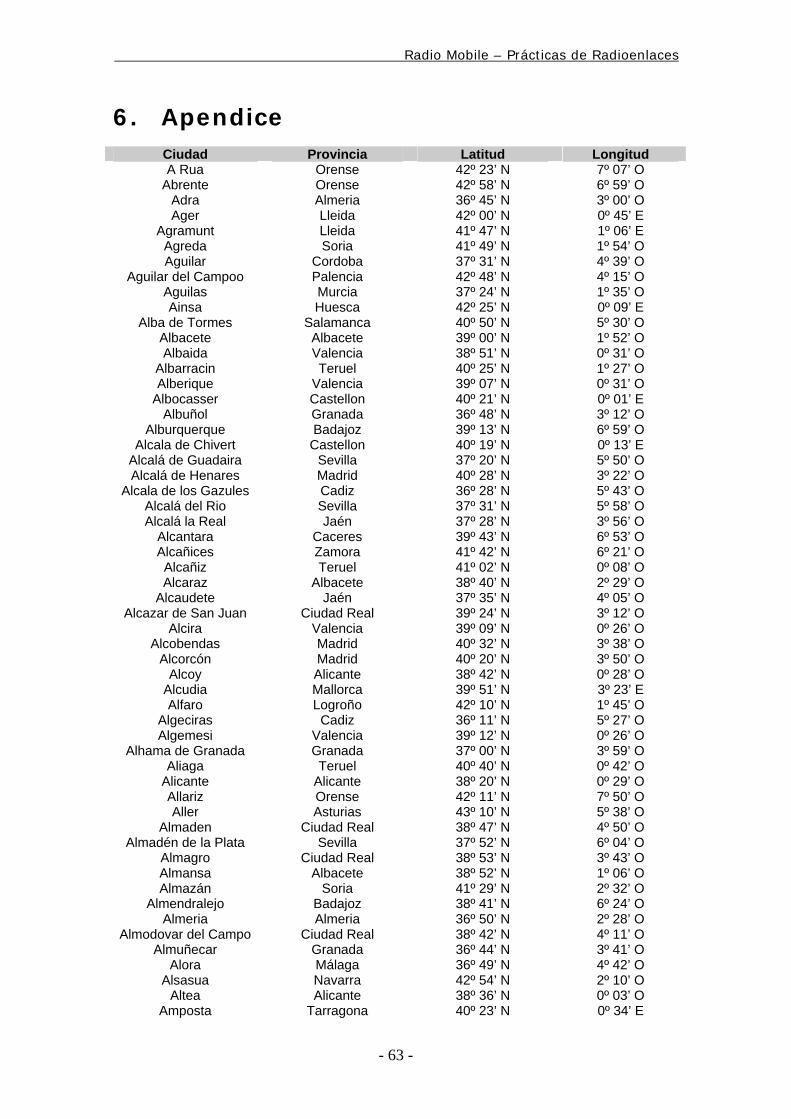
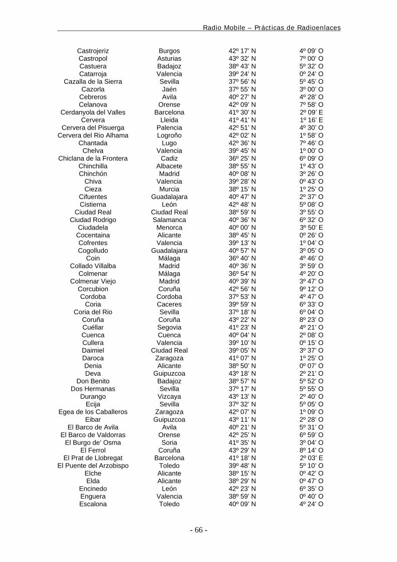
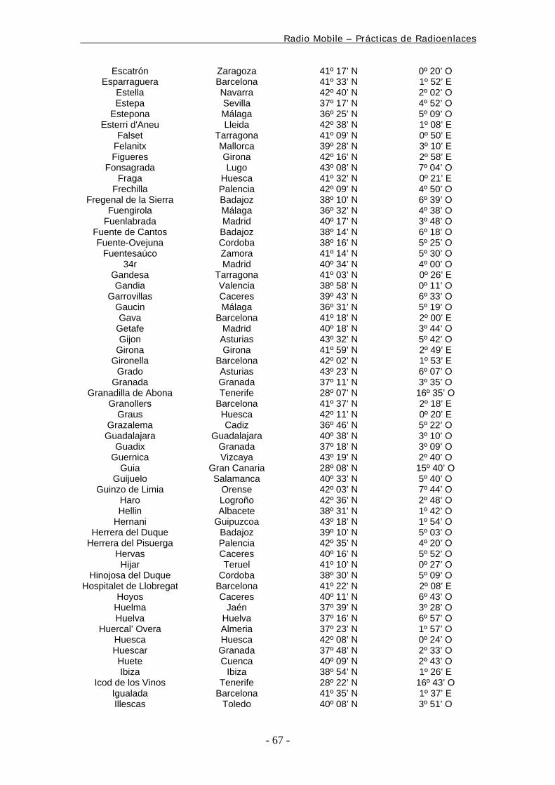
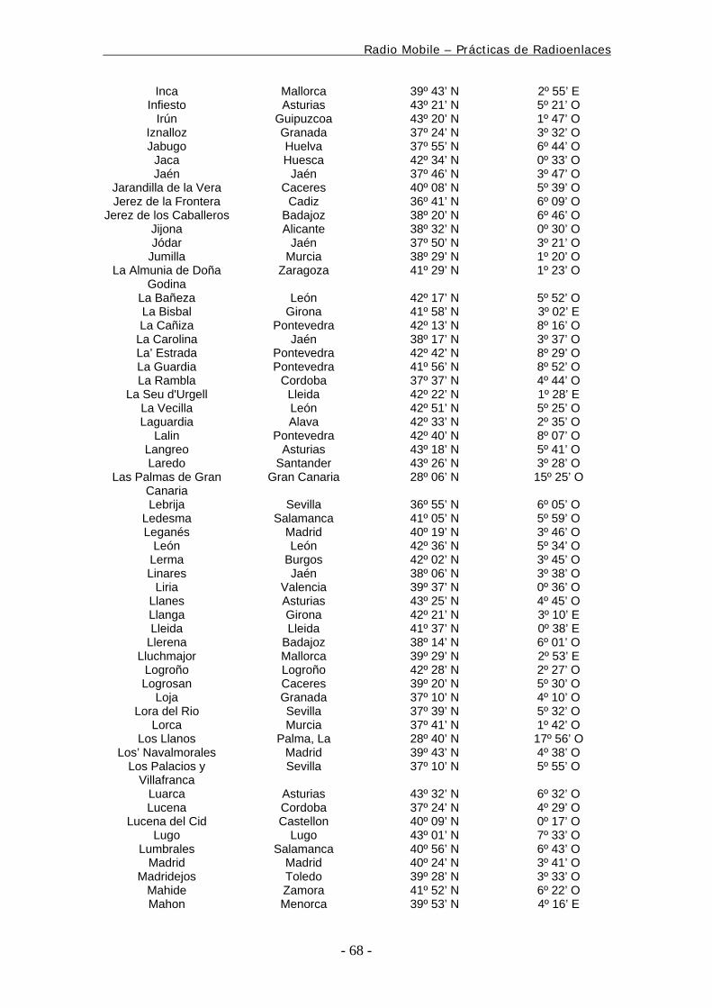
6. Apendice Ciudad Provincia Latitud Longitud A Rua Orense 42º 23’ N 7º 07’ O
Abrente Orense 42º 58’ N 6º 59’ O Adra Almeria 36º 45’ N 3º 00’ O Ager Lleida 42º 00’ N 0º 45’ E
Agramunt Lleida 41º 47’ N 1º 06’ E Agreda Soria 41º 49’ N 1º 54’ O Aguilar Cordoba 37º 31’ N 4º 39’ O
Aguilar del Campoo Palencia 42º 48’ N 4º 15’ O Aguilas Murcia 37º 24’ N 1º 35’ O Ainsa Huesca 42º 25’ N 0º 09’ E
Alba de Tormes Salamanca 40º 50’ N 5º 30’ O Albacete Albacete 39º 00’ N 1º 52’ O Albaida Valencia 38º 51’ N 0º 31’ O
Albarracin Teruel 40º 25’ N 1º 27’ O Alberique Valencia 39º 07’ N 0º 31’ O
Albocasser Castellon 40º 21’ N 0º 01’ E Albuñol Granada 36º 48’ N 3º 12’ O
Alburquerque Badajoz 39º 13’ N 6º 59’ O Alcala de Chivert Castellon 40º 19’ N 0º 13’ E
Alcalá de Guadaira Sevilla 37º 20’ N 5º 50’ O Alcalá de Henares Madrid 40º 28’ N 3º 22’ O
Alcala de los Gazules Cadiz 36º 28’ N 5º 43’ O Alcalá del Rio Sevilla 37º 31’ N 5º 58’ O Alcalá la Real Jaén 37º 28’ N 3º 56’ O
Alcantara Caceres 39º 43’ N 6º 53’ O Alcañices Zamora 41º 42’ N 6º 21’ O Alcañiz Teruel 41º 02’ N 0º 08’ O Alcaraz Albacete 38º 40’ N 2º 29’ O
Alcaudete Jaén 37º 35’ N 4º 05’ O Alcazar de San Juan Ciudad Real 39º 24’ N 3º 12’ O
Alcira Valencia 39º 09’ N 0º 26’ O Alcobendas Madrid 40º 32’ N 3º 38’ O
Alcorcón Madrid 40º 20’ N 3º 50’ O Alcoy Alicante 38º 42’ N 0º 28’ O
Alcudia Mallorca 39º 51’ N 3º 23’ E Alfaro Logroño 42º 10’ N 1º 45’ O
Algeciras Cadiz 36º 11’ N 5º 27’ O Algemesi Valencia 39º 12’ N 0º 26’ O
Alhama de Granada Granada 37º 00’ N 3º 59’ O Aliaga Teruel 40º 40’ N 0º 42’ O
Alicante Alicante 38º 20’ N 0º 29’ O Allariz Orense 42º 11’ N 7º 50’ O Aller Asturias 43º 10’ N 5º 38’ O
Almaden Ciudad Real 38º 47’ N 4º 50’ O Almadén de la Plata Sevilla 37º 52’ N 6º 04’ O
Almagro Ciudad Real 38º 53’ N 3º 43’ O Almansa Albacete 38º 52’ N 1º 06’ O Almazán Soria 41º 29’ N 2º 32’ O
Almendralejo Badajoz 38º 41’ N 6º 24’ O Almeria Almeria 36º 50’ N 2º 28’ O
Almodovar del Campo Ciudad Real 38º 42’ N 4º 11’ O Almuñecar Granada 36º 44’ N 3º 41’ O
Alora Málaga 36º 49’ N 4º 42’ O Alsasua Navarra 42º 54’ N 2º 10’ O
Altea Alicante 38º 36’ N 0º 03’ O Amposta Tarragona 40º 23’ N 0º 34’ E
Radio Mobile – Prácticas de Radioenlaces
- 64 -
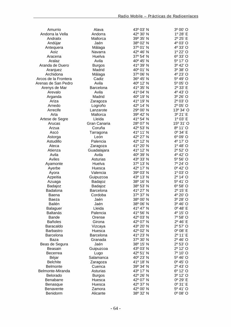
Amurrio Alava 43º 03’ N 3º 00’ O Andorra la Vella Andorra 42º 30’ N 1º 28’ E
Andraitx Mallorca 39º 35’ N 2º 25’ E Andújar Jaén 38º 02’ N 4º 03’ O
Antequera Málaga 37º 01’ N 4º 33’ O Aoiz Navarra 42º 46’ N 1º 22’ O
Aracena Huelva 37º 54’ N 6º 33’ O Aralaz Avila 40º 45’ N 5º 17’ O
Aranda de Duero Burgos 41º 39’ N 3º 42’ O Aranjuez Madrid 40º 01’ N 3º 38’ O Archidona Málaga 37º 06’ N 4º 23’ O
Arcos de la Frontera Cadiz 36º 45’ N 5º 49’ O Arenas de San Pedro Avila 40º 12’ N 5º 05’ O
Arenys de Mar Barcelona 41º 35’ N 2º 33’ E Arevalo Avila 41º 04’ N 4º 43’ O Arganda Madrid 40º 19’ N 3º 26’ O
Ariza Zaragoza 41º 19’ N 2º 03’ O Arnedo Logroño 42º 14’ N 2º 05’ O Arrecife Lanzarote 29º 00’ N 13º 34’ O
Arta Mallorca 39º 42’ N 3º 21’ E Artese de Segre Lleida 41º 54’ N 1º 03’ E
Arucas Gran Canaria 28º 07’ N 15º 31’ O Arzua Coruña 42º 53’ N 8º 11’ O Ascó Tarragona 41º 11’ N 0º 34’ E
Astorga León 42º 27’ N 6º 09’ O Astudillo Palencia 42º 12’ N 4º 17’ O
Ateca Zaragoza 41º 20’ N 1º 48’ O Atienza Guadalajara 41º 12’ N 2º 52’ O
Avila Avila 40º 39’ N 4º 42’ O Aviles Asturias 43º 33’ N 5º 56’ O
Ayamonte Huelva 37º 13’ N 7º 24’ O Ayerbe Huesca 42º 17’ N 0º 42’ O Ayora Valencia 39º 03’ N 1º 03’ O
Azpeitia Guipuzcoa 43º 13’ N 2º 14’ O Azuaga Badajoz 38º 16’ N 5º 41’ O Badajoz Badajoz 38º 53’ N 6º 58’ O
Badalona Barcelona 41º 27’ N 2º 15’ E Baena Cordoba 37º 37’ N 4º 20’ O Baeza Jaén 38º 00’ N 3º 28’ O Bailén Jaén 38º 06’ N 3º 46’ O
Balaguer Lleida 41º 47’ N 0º 48’ E Baltanás Palencia 41º 56’ N 4º 15’ O Bande Orense 42º 03’ N 7º 58’ O
Bañoles Girona 42º 07’ N 2º 46’ E Baracaldo Vizcaya 43º 20’ N 2º 57’ O Barbastro Huesca 42º 02’ N 0º 08’ E Barcelona Barcelona 41º 23’ N 2º 11’ E
Baza Granada 37º 30’ N 2º 46’ O Beas de Segura Jaén 38º 15’ N 2º 53’ O
Beasain Guipuzcoa 43º 03’ N 2º 12’ O Becerrea Lugo 42º 51’ N 7º 10’ O
Béjar Salamanca 40º 23’ N 5º 46’ O Belchite Zaragoza 41º 18’ N 0º 45’ O
Belmonte Cuenca 39º 34’ N 2º 43’ O Belmonte-Miranda Asturias 43º 17’ N 6º 12’ O
Belorado Burgos 42º 26’ N 3º 12’ O Benabarre Huesca 42º 07’ N 0º 29’ E Benasque Huesca 42º 37’ N 0º 31’ E Benavente Zamora 42º 00’ N 5º 41’ O Benidorm Alicante 38º 32’ N 0º 08’ O
Radio Mobile – Prácticas de Radioenlaces
- 65 -
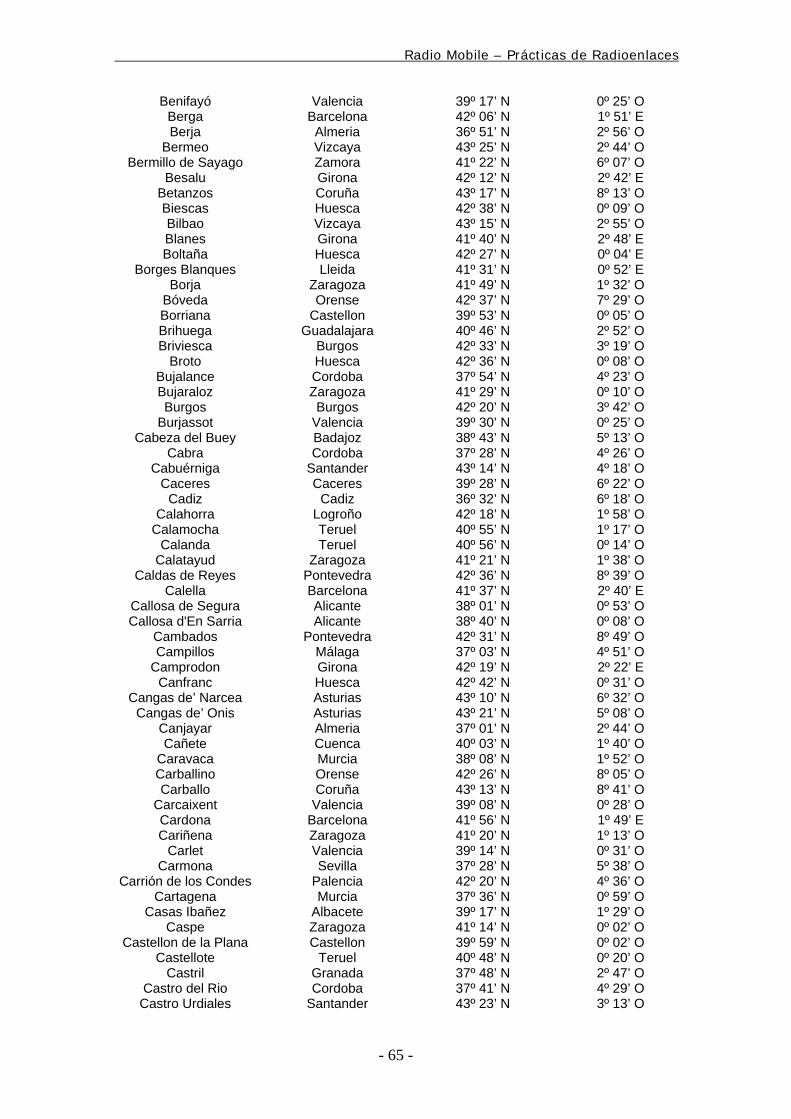
Benifayó Valencia 39º 17’ N 0º 25’ O Berga Barcelona 42º 06’ N 1º 51’ E Berja Almeria 36º 51’ N 2º 56’ O
Bermeo Vizcaya 43º 25’ N 2º 44’ O Bermillo de Sayago Zamora 41º 22’ N 6º 07’ O
Besalu Girona 42º 12’ N 2º 42’ E Betanzos Coruña 43º 17’ N 8º 13’ O Biescas Huesca 42º 38’ N 0º 09’ O Bilbao Vizcaya 43º 15’ N 2º 55’ O Blanes Girona 41º 40’ N 2º 48’ E Boltaña Huesca 42º 27’ N 0º 04’ E
Borges Blanques Lleida 41º 31’ N 0º 52’ E Borja Zaragoza 41º 49’ N 1º 32’ O
Bóveda Orense 42º 37’ N 7º 29’ O Borriana Castellon 39º 53’ N 0º 05’ O Brihuega Guadalajara 40º 46’ N 2º 52’ O Briviesca Burgos 42º 33’ N 3º 19’ O
Broto Huesca 42º 36’ N 0º 08’ O Bujalance Cordoba 37º 54’ N 4º 23’ O Bujaraloz Zaragoza 41º 29’ N 0º 10’ O Burgos Burgos 42º 20’ N 3º 42’ O
Burjassot Valencia 39º 30’ N 0º 25’ O Cabeza del Buey Badajoz 38º 43’ N 5º 13’ O
Cabra Cordoba 37º 28’ N 4º 26’ O Cabuérniga Santander 43º 14’ N 4º 18’ O
Caceres Caceres 39º 28’ N 6º 22’ O Cadiz Cadiz 36º 32’ N 6º 18’ O
Calahorra Logroño 42º 18’ N 1º 58’ O Calamocha Teruel 40º 55’ N 1º 17’ O
Calanda Teruel 40º 56’ N 0º 14’ O Calatayud Zaragoza 41º 21’ N 1º 38’ O
Caldas de Reyes Pontevedra 42º 36’ N 8º 39’ O Calella Barcelona 41º 37’ N 2º 40’ E
Callosa de Segura Alicante 38º 01’ N 0º 53’ O Callosa d'En Sarria Alicante 38º 40’ N 0º 08’ O
Cambados Pontevedra 42º 31’ N 8º 49’ O Campillos Málaga 37º 03’ N 4º 51’ O
Camprodon Girona 42º 19’ N 2º 22’ E Canfranc Huesca 42º 42’ N 0º 31’ O
Cangas de’ Narcea Asturias 43º 10’ N 6º 32’ O Cangas de’ Onis Asturias 43º 21’ N 5º 08’ O
Canjayar Almeria 37º 01’ N 2º 44’ O Cañete Cuenca 40º 03’ N 1º 40’ O
Caravaca Murcia 38º 08’ N 1º 52’ O Carballino Orense 42º 26’ N 8º 05’ O Carballo Coruña 43º 13’ N 8º 41’ O
Carcaixent Valencia 39º 08’ N 0º 28’ O Cardona Barcelona 41º 56’ N 1º 49’ E Cariñena Zaragoza 41º 20’ N 1º 13’ O
Carlet Valencia 39º 14’ N 0º 31’ O Carmona Sevilla 37º 28’ N 5º 38’ O
Carrión de los Condes Palencia 42º 20’ N 4º 36’ O Cartagena Murcia 37º 36’ N 0º 59’ O
Casas Ibañez Albacete 39º 17’ N 1º 29’ O Caspe Zaragoza 41º 14’ N 0º 02’ O
Castellon de la Plana Castellon 39º 59’ N 0º 02’ O Castellote Teruel 40º 48’ N 0º 20’ O
Castril Granada 37º 48’ N 2º 47’ O Castro del Rio Cordoba 37º 41’ N 4º 29’ O Castro Urdiales Santander 43º 23’ N 3º 13’ O
Radio Mobile – Prácticas de Radioenlaces
- 66 -
Castrojeriz Burgos 42º 17’ N 4º 09’ O Castropol Asturias 43º 32’ N 7º 00’ O Castuera Badajoz 38º 43’ N 5º 32’ O Catarroja Valencia 39º 24’ N 0º 24’ O
Cazalla de la Sierra Sevilla 37º 56’ N 5º 45’ O Cazorla Jaén 37º 55’ N 3º 00’ O
Cebreros Avila 40º 27’ N 4º 28’ O Celanova Orense 42º 09’ N 7º 58’ O
Cerdanyola del Valles Barcelona 41º 30’ N 2º 09’ E Cervera Lleida 41º 41’ N 1º 16’ E
Cervera del Pisuerga Palencia 42º 51’ N 4º 30’ O Cervera del Rio Alhama Logroño 42º 02’ N 1º 58’ O
Chantada Lugo 42º 36’ N 7º 46’ O Chelva Valencia 39º 45’ N 1º 00’ O
Chiclana de la Frontera Cadiz 36º 25’ N 6º 09’ O Chinchilla Albacete 38º 55’ N 1º 43’ O Chinchón Madrid 40º 08’ N 3º 26’ O
Chiva Valencia 39º 28’ N 0º 43’ O Cieza Murcia 38º 15’ N 1º 25’ O
Cifuentes Guadalajara 40º 47’ N 2º 37’ O Cistierna León 42º 48’ N 5º 08’ O
Ciudad Real Ciudad Real 38º 59’ N 3º 55’ O Ciudad Rodrigo Salamanca 40º 36’ N 6º 32’ O
Ciudadela Menorca 40º 00’ N 3º 50’ E Cocentaina Alicante 38º 45’ N 0º 26’ O Cofrentes Valencia 39º 13’ N 1º 04’ O Cogolludo Guadalajara 40º 57’ N 3º 05’ O
Coin Málaga 36º 40’ N 4º 46’ O Collado Villalba Madrid 40º 36’ N 3º 59’ O
Colmenar Málaga 36º 54’ N 4º 20’ O Colmenar Viejo Madrid 40º 39’ N 3º 47’ O
Corcubion Coruña 42º 56’ N 9º 12’ O Cordoba Cordoba 37º 53’ N 4º 47’ O
Coria Caceres 39º 59’ N 6º 33’ O Coria del Rio Sevilla 37º 18’ N 6º 04’ O
Coruña Coruña 43º 22’ N 8º 23’ O Cuéllar Segovia 41º 23’ N 4º 21’ O Cuenca Cuenca 40º 04’ N 2º 08’ O Cullera Valencia 39º 10’ N 0º 15’ O Daimiel Ciudad Real 39º 05’ N 3º 37’ O Daroca Zaragoza 41º 07’ N 1º 25’ O Denia Alicante 38º 50’ N 0º 07’ O Deva Guipuzcoa 43º 18’ N 2º 21’ O
Don Benito Badajoz 38º 57’ N 5º 52’ O Dos Hermanas Sevilla 37º 17’ N 5º 55’ O
Durango Vizcaya 43º 13’ N 2º 40’ O Ecija Sevilla 37º 32’ N 5º 05’ O
Egea de los Caballeros Zaragoza 42º 07’ N 1º 09’ O Eibar Guipuzcoa 43º 11’ N 2º 28’ O
El Barco de Avila Avila 40º 21’ N 5º 31’ O El Barco de Valdorras Orense 42º 25’ N 6º 59’ O
El Burgo de’ Osma Soria 41º 35’ N 3º 04’ O El Ferrol Coruña 43º 29’ N 8º 14’ O
El Prat de Llobregat Barcelona 41º 18’ N 2º 03’ E El Puente del Arzobispo Toledo 39º 48’ N 5º 10’ O
Elche Alicante 38º 15’ N 0º 42’ O Elda Alicante 38º 29’ N 0º 47’ O
Encinedo León 42º 23’ N 6º 35’ O Enguera Valencia 38º 59’ N 0º 40’ O Escalona Toledo 40º 09’ N 4º 24’ O
Radio Mobile – Prácticas de Radioenlaces
- 67 -
Escatrón Zaragoza 41º 17’ N 0º 20’ O Esparraguera Barcelona 41º 33’ N 1º 52’ E
Estella Navarra 42º 40’ N 2º 02’ O Estepa Sevilla 37º 17’ N 4º 52’ O
Estepona Málaga 36º 25’ N 5º 09’ O Esterri d'Aneu Lleida 42º 38’ N 1º 08’ E
Falset Tarragona 41º 09’ N 0º 50’ E Felanitx Mallorca 39º 28’ N 3º 10’ E Figueres Girona 42º 16’ N 2º 58’ E
Fonsagrada Lugo 43º 08’ N 7º 04’ O Fraga Huesca 41º 32’ N 0º 21’ E
Frechilla Palencia 42º 09’ N 4º 50’ O Fregenal de la Sierra Badajoz 38º 10’ N 6º 39’ O
Fuengirola Málaga 36º 32’ N 4º 38’ O Fuenlabrada Madrid 40º 17’ N 3º 48’ O
Fuente de Cantos Badajoz 38º 14’ N 6º 18’ O Fuente-Ovejuna Cordoba 38º 16’ N 5º 25’ O
Fuentesaúco Zamora 41º 14’ N 5º 30’ O 34r Madrid 40º 34’ N 4º 00’ O
Gandesa Tarragona 41º 03’ N 0º 26’ E Gandia Valencia 38º 58’ N 0º 11’ O
Garrovillas Caceres 39º 43’ N 6º 33’ O Gaucin Málaga 36º 31’ N 5º 19’ O Gava Barcelona 41º 18’ N 2º 00’ E
Getafe Madrid 40º 18’ N 3º 44’ O Gijon Asturias 43º 32’ N 5º 42’ O
Girona Girona 41º 59’ N 2º 49’ E Gironella Barcelona 42º 02’ N 1º 53’ E
Grado Asturias 43º 23’ N 6º 07’ O Granada Granada 37º 11’ N 3º 35’ O
Granadilla de Abona Tenerife 28º 07’ N 16º 35’ O Granollers Barcelona 41º 37’ N 2º 18’ E
Graus Huesca 42º 11’ N 0º 20’ E Grazalema Cadiz 36º 46’ N 5º 22’ O Guadalajara Guadalajara 40º 38’ N 3º 10’ O
Guadix Granada 37º 18’ N 3º 09’ O Guernica Vizcaya 43º 19’ N 2º 40’ O
Guia Gran Canaria 28º 08’ N 15º 40’ O Guijuelo Salamanca 40º 33’ N 5º 40’ O
Guinzo de Limia Orense 42º 03’ N 7º 44’ O Haro Logroño 42º 36’ N 2º 48’ O Hellin Albacete 38º 31’ N 1º 42’ O
Hernani Guipuzcoa 43º 18’ N 1º 54’ O Herrera del Duque Badajoz 39º 10’ N 5º 03’ O
Herrera del Pisuerga Palencia 42º 35’ N 4º 20’ O Hervas Caceres 40º 16’ N 5º 52’ O Hijar Teruel 41º 10’ N 0º 27’ O
Hinojosa del Duque Cordoba 38º 30’ N 5º 09’ O Hospitalet de Llobregat Barcelona 41º 22’ N 2º 08’ E
Hoyos Caceres 40º 11’ N 6º 43’ O Huelma Jaén 37º 39’ N 3º 28’ O Huelva Huelva 37º 16’ N 6º 57’ O
Huercal’ Overa Almeria 37º 23’ N 1º 57’ O Huesca Huesca 42º 08’ N 0º 24’ O Huescar Granada 37º 48’ N 2º 33’ O Huete Cuenca 40º 09’ N 2º 43’ O Ibiza Ibiza 38º 54’ N 1º 26’ E
Icod de los Vinos Tenerife 28º 22’ N 16º 43’ O Igualada Barcelona 41º 35’ N 1º 37’ E Illescas Toledo 40º 08’ N 3º 51’ O
Radio Mobile – Prácticas de Radioenlaces
- 68 -
Inca Mallorca 39º 43’ N 2º 55’ E Infiesto Asturias 43º 21’ N 5º 21’ O
Irún Guipuzcoa 43º 20’ N 1º 47’ O Iznalloz Granada 37º 24’ N 3º 32’ O Jabugo Huelva 37º 55’ N 6º 44’ O
Jaca Huesca 42º 34’ N 0º 33’ O Jaén Jaén 37º 46’ N 3º 47’ O
Jarandilla de la Vera Caceres 40º 08’ N 5º 39’ O Jerez de la Frontera Cadiz 36º 41’ N 6º 09’ O
Jerez de los Caballeros Badajoz 38º 20’ N 6º 46’ O Jijona Alicante 38º 32’ N 0º 30’ O Jódar Jaén 37º 50’ N 3º 21’ O
Jumilla Murcia 38º 29’ N 1º 20’ O La Almunia de Doña
Godina Zaragoza 41º 29’ N 1º 23’ O
La Bañeza León 42º 17’ N 5º 52’ O La Bisbal Girona 41º 58’ N 3º 02’ E La Cañiza Pontevedra 42º 13’ N 8º 16’ O
La Carolina Jaén 38º 17’ N 3º 37’ O La’ Estrada Pontevedra 42º 42’ N 8º 29’ O La Guardia Pontevedra 41º 56’ N 8º 52’ O La Rambla Cordoba 37º 37’ N 4º 44’ O
La Seu d'Urgell Lleida 42º 22’ N 1º 28’ E La Vecilla León 42º 51’ N 5º 25’ O Laguardia Alava 42º 33’ N 2º 35’ O
Lalin Pontevedra 42º 40’ N 8º 07’ O Langreo Asturias 43º 18’ N 5º 41’ O Laredo Santander 43º 26’ N 3º 28’ O
Las Palmas de Gran Canaria
Gran Canaria 28º 06’ N 15º 25’ O
Lebrija Sevilla 36º 55’ N 6º 05’ O Ledesma Salamanca 41º 05’ N 5º 59’ O Leganés Madrid 40º 19’ N 3º 46’ O
León León 42º 36’ N 5º 34’ O Lerma Burgos 42º 02’ N 3º 45’ O Linares Jaén 38º 06’ N 3º 38’ O
Liria Valencia 39º 37’ N 0º 36’ O Llanes Asturias 43º 25’ N 4º 45’ O Llanga Girona 42º 21’ N 3º 10’ E Lleida Lleida 41º 37’ N 0º 38’ E
Llerena Badajoz 38º 14’ N 6º 01’ O Lluchmajor Mallorca 39º 29’ N 2º 53’ E
Logroño Logroño 42º 28’ N 2º 27’ O Logrosan Caceres 39º 20’ N 5º 30’ O
Loja Granada 37º 10’ N 4º 10’ O Lora del Rio Sevilla 37º 39’ N 5º 32’ O
Lorca Murcia 37º 41’ N 1º 42’ O Los Llanos Palma, La 28º 40’ N 17º 56’ O
Los’ Navalmorales Madrid 39º 43’ N 4º 38’ O Los Palacios y
Villafranca Sevilla 37º 10’ N 5º 55’ O
Luarca Asturias 43º 32’ N 6º 32’ O Lucena Cordoba 37º 24’ N 4º 29’ O
Lucena del Cid Castellon 40º 09’ N 0º 17’ O Lugo Lugo 43º 01’ N 7º 33’ O
Lumbrales Salamanca 40º 56’ N 6º 43’ O Madrid Madrid 40º 24’ N 3º 41’ O
Madridejos Toledo 39º 28’ N 3º 33’ O Mahide Zamora 41º 52’ N 6º 22’ O Mahon Menorca 39º 53’ N 4º 16’ E
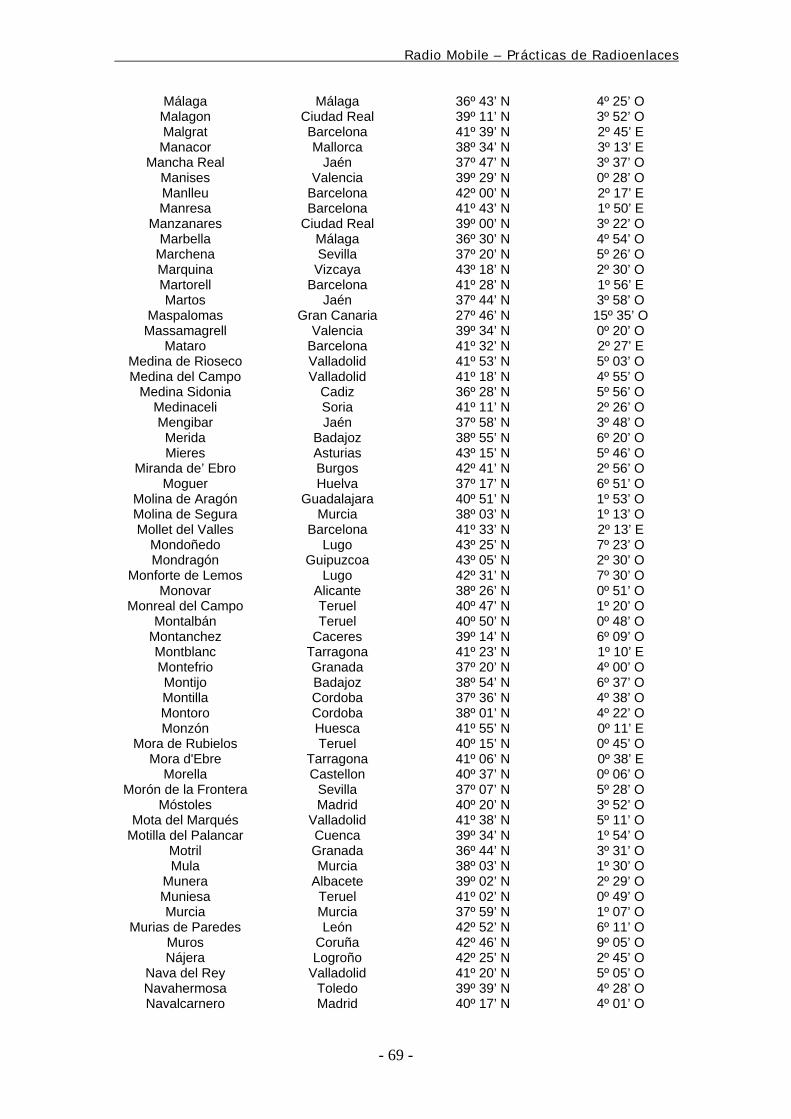
Radio Mobile – Prácticas de Radioenlaces
- 69 -
Málaga Málaga 36º 43’ N 4º 25’ O Malagon Ciudad Real 39º 11’ N 3º 52’ O Malgrat Barcelona 41º 39’ N 2º 45’ E Manacor Mallorca 38º 34’ N 3º 13’ E
Mancha Real Jaén 37º 47’ N 3º 37’ O Manises Valencia 39º 29’ N 0º 28’ O Manlleu Barcelona 42º 00’ N 2º 17’ E Manresa Barcelona 41º 43’ N 1º 50’ E
Manzanares Ciudad Real 39º 00’ N 3º 22’ O Marbella Málaga 36º 30’ N 4º 54’ O
Marchena Sevilla 37º 20’ N 5º 26’ O Marquina Vizcaya 43º 18’ N 2º 30’ O Martorell Barcelona 41º 28’ N 1º 56’ E Martos Jaén 37º 44’ N 3º 58’ O
Maspalomas Gran Canaria 27º 46’ N 15º 35’ O Massamagrell Valencia 39º 34’ N 0º 20’ O
Mataro Barcelona 41º 32’ N 2º 27’ E Medina de Rioseco Valladolid 41º 53’ N 5º 03’ O Medina del Campo Valladolid 41º 18’ N 4º 55’ O
Medina Sidonia Cadiz 36º 28’ N 5º 56’ O Medinaceli Soria 41º 11’ N 2º 26’ O Mengibar Jaén 37º 58’ N 3º 48’ O
Merida Badajoz 38º 55’ N 6º 20’ O Mieres Asturias 43º 15’ N 5º 46’ O
Miranda de’ Ebro Burgos 42º 41’ N 2º 56’ O Moguer Huelva 37º 17’ N 6º 51’ O
Molina de Aragón Guadalajara 40º 51’ N 1º 53’ O Molina de Segura Murcia 38º 03’ N 1º 13’ O Mollet del Valles Barcelona 41º 33’ N 2º 13’ E
Mondoñedo Lugo 43º 25’ N 7º 23’ O Mondragón Guipuzcoa 43º 05’ N 2º 30’ O
Monforte de Lemos Lugo 42º 31’ N 7º 30’ O Monovar Alicante 38º 26’ N 0º 51’ O
Monreal del Campo Teruel 40º 47’ N 1º 20’ O Montalbán Teruel 40º 50’ N 0º 48’ O
Montanchez Caceres 39º 14’ N 6º 09’ O Montblanc Tarragona 41º 23’ N 1º 10’ E Montefrio Granada 37º 20’ N 4º 00’ O Montijo Badajoz 38º 54’ N 6º 37’ O Montilla Cordoba 37º 36’ N 4º 38’ O Montoro Cordoba 38º 01’ N 4º 22’ O Monzón Huesca 41º 55’ N 0º 11’ E
Mora de Rubielos Teruel 40º 15’ N 0º 45’ O Mora d'Ebre Tarragona 41º 06’ N 0º 38’ E
Morella Castellon 40º 37’ N 0º 06’ O Morón de la Frontera Sevilla 37º 07’ N 5º 28’ O
Móstoles Madrid 40º 20’ N 3º 52’ O Mota del Marqués Valladolid 41º 38’ N 5º 11’ O
Motilla del Palancar Cuenca 39º 34’ N 1º 54’ O Motril Granada 36º 44’ N 3º 31’ O Mula Murcia 38º 03’ N 1º 30’ O
Munera Albacete 39º 02’ N 2º 29’ O Muniesa Teruel 41º 02’ N 0º 49’ O Murcia Murcia 37º 59’ N 1º 07’ O
Murias de Paredes León 42º 52’ N 6º 11’ O Muros Coruña 42º 46’ N 9º 05’ O Nájera Logroño 42º 25’ N 2º 45’ O
Nava del Rey Valladolid 41º 20’ N 5º 05’ O Navahermosa Toledo 39º 39’ N 4º 28’ O Navalcarnero Madrid 40º 17’ N 4º 01’ O
Radio Mobile – Prácticas de Radioenlaces
- 70 -
Navalmoral de la Mata Caceres 39º 53’ N 5º 33’ O Navia Asturias 43º 33’ N 6º 42’ O
Negreira Coruña 42º 54’ N 8º 45’ O Nerja Málaga 36º 44’ N 3º 53’ O
Nerpio Albacete 38º 08’ N 2º 18’ O Nijar Almeria 36º 58’ N 2º 12’ O
Nonaspe Zaragoza 41º 13’ N 0º 02’ E Novelda Alicante 38º 23’ N 0º 45’ O
Noya Coruña 42º 48’ N 8º 53’ O Nules Castellon 39º 51’ N 0º 09’ O Ocaña Toledo 39º 57’ N 3º 30’ O Oliva Valencia 38º 55’ N 0º 07’ O
Olivenza Badajoz 38º 41’ N 7º 06’ O Olmedo Valladolid 41º 17’ N 4º 41’ O
Olot Girona 42º 11’ N 2º 30’ E Olvera Cadiz 36º 56’ N 5º 16’ O Onda Castellon 39º 58’ N 0º 15’ O
Onteniente Valencia 38º 50’ N 0º 36’ O Orcera Jaén 38º 19’ N 2º 39’ O
Ordenes Coruña 43º 05’ N 8º 24’ O Orense Orense 42º 20’ N 7º 52’ O Orgaz Toledo 39º 39’ N 3º 53’ O Orgiva Granada 36º 54’ N 3º 26’ O
Orihuela Alicante 38º 05’ N 0º 57’ O Oropesa Castellon 40º 06’ N 0º 09’ E Osuna Sevilla 37º 14’ N 5º 07’ O Oviedo Asturias 43º 22’ N 5º 50’ O Padron Coruña 42º 44’ N 8º 39’ O
Palafrugell Girona 41º 55’ N 3º 10’ E Palamos Girona 41º 51’ N 3º 08’ E Palencia Palencia 42º 00’ N 4º 32’ O
Palma de Mallorca Mallorca 39º 35’ N 2º 39’ E Palma del Condado Huelva 37º 23’ N 6º 35’ O
Palma del Rio Cordoba 37º 42’ N 5º 17’ O Pamplona Navarra 42º 49’ N 1º 38’ O
Paramo del Sil León 42º 48’ N 6º 29’ O Pastrana Guadalajara 40º 25’ N 2º 55’ O Paterna Valencia 39º 30’ N 0º 26’ O
Pego Alicante 38º 51’ N 0º 08’ O Peñafiel Valladolid 41º 36’ N 4º 07’ O
Peñaranda de Bracamonte
Salamanca 40º 54’ N 5º 13’ O
Peñarroya-Pueblonuevo Cordoba 38º 19’ N 5º 16’ O Perelló Tarragona 40º 52’ N 0º 43’ E
Piedrabuena Ciudad Real 39º 02’ N 4º 10’ O Piedrahita Avila 40º 28’ N 5º 20’ O
Pina de’ Ebro Zaragoza 41º 29’ N 0º 32’ O Pinos Puente Granada 37º 15’ N 3º 45’ O
Pinto Madrid 40º 14’ N 3º 43’ O Plasencia Caceres 40º 02’ N 6º 06’ O
Pobla de Segur Lleida 42º 15’ N 0º 58’ E Pola de Lena Asturias 43º 10’ N 5º 49’ O Pola de Siero Asturias 43º 24’ N 5º 39’ O Ponferrada León 42º 33’ N 6º 35’ O
Pont de Suert Lleida 42º 25’ N 0º 45’ E Pontedeume Coruña 43º 24’ N 8º 10’ O Pontevedra Pontevedra 42º 26’ N 8º 39’ O
Porcuna Jaén 37º 52’ N 4º 11’ O Porriño Pontevedra 42º 12’ N 8º 39’ O
Posadas Cordoba 37º 48’ N 5º 07’ O
Radio Mobile – Prácticas de Radioenlaces
- 71 -
Potes Santander 43º 10’ N 4º 37’ O Pozoblanco Cordoba 38º 23’ N 4º 51’ O
Pravia Asturias 43º 30’ N 6º 07’ O Priego de Cordoba Cordoba 37º 26’ N 4º 12’ O Puebla de Alcocer Badajoz 38º 59’ N 5º 15’ O Puebla de Guzmán Huelva 37º 37’ N 7º 15’ O Puebla de Sanabria Zamora 42º 03’ N 6º 39’ O
Puebla de Trives Orense 42º 20’ N 7º 15’ O Puente de la Reina Navarra 42º 40’ N 1º 49’ O
Puente Genil Cordoba 37º 23’ N 4º 46’ O Puenteáreas Pontevedra 42º 10’ N 8º 28’ O
Puentes de Garcia Rodriguez
Coruña 43º 27’ N 7º 51’ O
Puerto de la Cruz Tenerife 28º 25’ N 16º 33’ O Puerto de Santa Maria Cadiz 36º 36’ N 6º 13’ O
Puerto del Rosario Fuerteventura 28º 30’ N 13º 53’ O Puertollano Ciudad Real 38º 42’ N 4º 07’ O Puigcerda Girona 42º 26’ N 1º 56’ E Purchena Almeria 37º 21’ N 2º 21’ O Quesada Jaén 37º 51’ N 3º 05’ O
Quintanar de la’ Orden Toledo 39º 35’ N 3º 03’ O Quiroga Lugo 42º 28’ N 7º 15’ O
Ramales de la Victoria Santander 43º 15’ N 3º 28’ O Redondela Pontevedra 42º 17’ N 8º 37’ O
Reinosa Santader 43º 00’ N 4º 08’ O Renteria Guipuzcoa 43º 17’ N 1º 58’ O Requena Valencia 39º 30’ N 1º 06’ O
Reus Tarragona 41º 10’ N 1º 06’ E Riaño León 42º 59’ N 5º 00’ O Riaza Segovia 41º 18’ N 3º 30’ O
Ribadavia Orense 42º 17’ N 8º 08’ O Ribadeo Lugo 43º 32’ N 7º 03’ O
Ribadesella Asturias 43º 28’ N 5º 07’ O Ribeira Coruña 42º 34’ N 8º 59’ O Ripoll Girona 42º 12’ N 2º 12’ E
Roncal Navarra 42º 50’ N 0º 55’ O Roncesvalles Navarra 43º 01’ N 1º 20’ O
Ronda Málaga 36º 45’ N 5º 10’ O Roquetas de Mar Almeria 36º 46’ N 2º 37’ O
Roses Girona 42º 16’ N 3º 11’ E Rute Cordoba 37º 19’ N 4º 23’ O
Sabadell Barcelona 41º 33’ N 2º 07’ E Sabiñánigo Huesca 42º 31’ N 0º 22’ O Sacedón Guadalajara 40º 29’ N 2º 44’ O Sádaba Zaragoza 42º 17’ N 1º 16’ O Sagunto Valencia 39º 41’ N 0º 16’ O Sahagún León 42º 22’ N 5º 02’ O
Salamanca Salamanca 40º 57’ N 5º 40’ O Salas de los Infantes Burgos 42º 03’ N 3º 16’ O
Saldaña Palencia 42º 32’ N 4º 44’ O Sallent Barcelona 41º 50’ N 1º 54’ E
San Antonio Ibiza 38º 59’ N 1º 19’ E San Bartolome de
Tirajana Gran Canaria 27º 56’ N 15º 35’ O
San Clemente Cuenca 39º 23’ N 2º 24’ O San Fernando Cadiz 36º 28’ N 6º 11’ O
San Javier Murcia 37º 49’ N 0º 50’ O San Juan Ibiza 39º 05’ N 1º 31’ E
San Lorenzo del’ Escorial
Madrid 40º 35’ N 4º 05’ O
Radio Mobile – Prácticas de Radioenlaces
- 72 -
San Martin de Valdeiglesias
Madrid 40º 21’ N 4º 24’ O
San Mateo Castellon 40º 28’ N 0º 11’ E San Roque Cadiz 36º 13’ N 5º 23’ O
San Sebastián Guipuzcoa 43º 19’ N 1º 59’ O San Sebastian de la
Gomera Gomera, La 28º 05’ N 17º 08’ O
San Sebastián de los Reyes
Madrid 40º 35’ N 3º 30’ O
San Vicente de la Barquera
Santander 43º 24’ N 4º 24’ O
Sangenjo Pontevedra 42º 24’ N 8º 48’ O Sangüesa Navarra 42º 35’ N 1º 17’ O
Sanlucar de Barrameda Cadiz 36º 46’ N 6º 21’ O Sanlúcar La Mayor Sevilla 37º 24’ N 6º 12’ O
Sant Boi de Llobregat Barcelona 41º 20’ N 2º 03’ E Sant Celoni Barcelona 41º 42’ N 2º 30’ E
Sant Feliu de Guixols Girona 41º 47’ N 3º 02’ E Sant Feliu de Llobregat Barcelona 41º 23’ N 2º 03’ E Sant Sadurni d'Anoia Barcelona 41º 26’ N 1º 47’ E
Santa Bárbara Tarragona 40º 43’ N 0º 30’ E Santa Coloma de
Farnés Girona 41º 52’ N 2º 40’ E
Santa Coloma de Gramanet
Barcelona 41º 27’ N 2º 13’ E
Santa Cruz de la Palma Palma, La 28º 41’ N 17º 45’ O Santa Cruz de Mudela Ciudad Real 38º 39’ N 3º 28’ O Santa Cruz de Tenerife Tenerife 28º 28’ N 16º 15’ O
Santa Fé Granada 37º 11’ N 3º 43’ O Santa Helena Jaén 38º 20’ N 3º 83’ O
Santa Maria de’ Ortigueira
Coruña 43º 41’ N 7º 50’ O
Santa Maria la Real de’ Nieva
Segovia 41º 04’ N 4º 24’ O
Santa Pau Girona 42º 09’ N 2º 35’ E Santander Santander 43º 28’ N 3º 48’ O
Santiago de Compostela
Coruña 42º 52’ N 8º 33’ O
Santo Domingo de la Calzada
Logroño 42º 26’ N 2º 57’ O
Santoña Santander 43º 27’ N 3º 29’ O Sariñena Huesca 41º 47’ N 0º 10’ O Sarreaus Orense 42º 05’ N 7º 36’ O
Sarria Lugo 42º 47’ N 7º 25’ O Sarriá de Ter Girona 42º 01’ N 2º 49’ E
Sedano Burgos 42º 43’ N 3º 45’ O Segorbe Castellon 39º 51’ N 0º 29’ O Segovia Segovia 40º 57’ N 4º 07’ O
Sepúlveda Segovia 41º 18’ N 3º 43’ O Sequeros Salamanca 40º 31’ N 6º 02’ O
Sevilla Sevilla 37º 23’ N 5º 59’ O Siguenza Guadalajara 41º 04’ N 2º 39’ O
Silla Valencia 39º 22’ N 0º 24’ O Sitges Barcelona 41º 14’ N 1º 48’ E
Socuellanos Ciudad Real 39º 17’ N 2º 47’ O Soller Mallorca 39º 46’ N 2º 43’ E
Solsona Lleida 42º 00’ N 1º 31’ E Sorbas Almeria 37º 06’ N 2º 08’ O Soria Soria 41º 46’ N 2º 28’ O Sort Lleida 42º 25’ N 1º 08’ E
Radio Mobile – Prácticas de Radioenlaces
- 73 -
Sos del Rey Católico Zaragoza 42º 29’ N 1º 12’ O Sueca Valencia 39º 12’ N 0º 20’ O Tafalla Navarra 42º 30’ N 1º 42’ O
Talavera de la Reina Toledo 39º 58’ N 4º 50’ O Tamarite de Litera Huesca 41º 52’ N 0º 25’ E
Tarancon Cuenca 40º 01’ N 3º 01’ O Tarazona Zaragoza 41º 54’ N 1º 43’ O
Tarifa Cadiz 36º 01’ N 5º 37’ O Tarragona Tarragona 41º 07’ N 1º 16’ E
Tárrega Lleida 41º 39’ N 1º 09’ E Tauste Zaragoza 41º 56’ N 1º 15’ O Telde Gran Canaria 27º 58’ N 15º 25’ O
Terrassa Barcelona 41º 34’ N 2º 01’ E Teruel Teruel 40º 20’ N 1º 06’ O Tineo Asturias 43º 20’ N 6º 25’ O Toledo Toledo 39º 51’ N 4º 01’ O Tolosa Guipuzcoa 43º 08’ N 2º 05’ O
Tomelloso Ciudad Real 39º 10’ N 3º 02’ O Tordesillas Valladolid 41º 30’ N 5º 00’ O
Toro Zamora 41º 31’ N 5º 24’ O Torrecilla’ En Cameros Logroño 42º 15’ N 2º 37’ O
Torrejón de Ardoz Madrid 40º 27’ N 3º 29’ O Torrelaguna Madrid 40º 50’ N 3º 35’ O Torrelavega Santander 43º 20’ N 4º 02’ O Torremolinos Málaga 36º 38’ N 4º 30’ O
Torrent de l'Horta Valencia 39º 26’ N 0º 28’ O Torrevieja Alicante 37º 59’ N 0º 40’ O
Torrijas Teruel 40º 02’ N 0º 57’ O Torrijos Toledo 39º 59’ N 4º 17’ O Torrox Málaga 36º 46’ N 3º 57’ O Tortosa Tarragona 40º 49’ N 0º 31’ E Totana Murcia 37º 46’ N 1º 30’ O Tremp Lleida 42º 10’ N 0º 54’ E Trujillo Caceres 39º 28’ N 5º 53’ O Tudela Navarra 42º 04’ N 1º 36’ O
Tuy Pontevedra 42º 03’ N 8º 39’ O Ubeda Jaén 38º 01’ N 3º 23’ O Ugijar Granada 36º 58’ N 3º 03’ O Utiel Valencia 39º 34’ N 1º 12’ O
Utrera Sevilla 37º 11’ N 5º 46’ O Valdepeñas Ciudad Real 38º 46’ N 3º 25’ O Valderrobles Teruel 40º 52’ N 0º 10’ E
Valencia Valencia 39º 28’ N 0º 22’ O Valencia de Alcantara Caceres 39º 25’ N 7º 14’ O Valencia de Don Juan León 42º 17’ N 5º 31’ O
Valladolid Valladolid 41º 39’ N 4º 44’ O Valls Tarragona 41º 17’ N 1º 15’ E
Valmaseda Vizcaya 43º 12’ N 3º 14’ O Valoria la Buena Valladolid 41º 48’ N 4º 32’ O
Valverde Hierro 27º 48’ N 17º 54’ O Valverde del Camino Huelva 37º 35’ N 6º 45’ O Vejer de la Frontera Cadiz 36º 15’ N 5º 58’ O
Vélez Málaga Málaga 36º 47’ N 4º 05’ O Velez Rubio Almeria 37º 39’ N 2º 05’ O
Vendrell Tarragona 41º 13’ N 1º 32’ E Venta de Baños Palencia 41º 56’ N 4º 30’ O
Vera Almeria 37º 15’ N 1º 53’ O Vergara Guipuzcoa 43º 07’ N 2º 25’ O
Verin Orense 41º 57’ N 7º 27’ O Viana del Bollo Orense 42º 11’ N 7º 07’ O
Radio Mobile – Prácticas de Radioenlaces
- 74 -
Vic Barcelona 41º 56’ N 2º 15’ E Viella Lleida 42º 42’ N 0º 48’ E Vigo Pontevedra 42º 15’ N 8º 43’ O
Vilafranca del Penedes Barcelona 41º 22’ N 1º 41’ E Vilanova i la Geltru Barcelona 41º 13’ N 1º 43’ E
Villablino León 42º 56’ N 6º 19’ O Villacarriedo Santander 43º 14’ N 3º 48’ O Villacarrillo Jaén 38º 07’ N 3º 05’ O Villacastin Segovia 40º 47’ N 4º 25’ O Villadiego Burgos 42º 31’ N 4º 01’ O
Villafranca del Bierzo León 42º 37’ N 6º 49’ O Villagarcia de Arosa Pontevedra 42º 36’ N 8º 46’ O
Villajoyosa Alicante 38º 30’ N 0º 14’ O Villalba Lugo 43º 17’ N 7º 41’ O
Villalón de Campos Valladolid 42º 06’ N 5º 02’ O Villalpando Zamora 41º 52’ N 5º 25’ O
Villanueva de la Serena Badajoz 38º 59’ N 5º 48’ O Villanueva de los
Infantes Ciudad Real 38º 44’ N 3º 01’ O
Villanueva del Fresno Badajoz 38º 23’ N 7º 10’ O Villar del Arzobispo Valencia 39º 44’ N 0º 50’ O
Villarcayo Burgos 42º 56’ N 3º 34’ O Villarreal de los Infantes Castellon 39º 56’ N 0º 06’ O
Villarrobledo Albacete 39º 16’ N 2º 36’ O Villaviciosa Asturias 43º 28’ N 5º 27’ O
Villena Alicante 38º 39’ N 0º 52’ O Vinaroz Castellon 40º 28’ N 0º 29’ E
Vitigudino Salamanca 41º 01’ N 6º 26’ O Vitoria Alava 42º 51’ N 2º 41’ O Viver Castellon 39º 55’ N 0º 36’ O Vivero Lugo 43º 39’ N 7º 38’ O Xátiva Valencia 39º 00’ N 0º 31’ O Yecla Murcia 38º 37’ N 1º 07’ O Yeste Albacete 38º 22’ N 2º 19’ O Zafra Badajoz 38º 26’ N 6º 25’ O
Zamora Zamora 41º 30’ N 5º 45’ O Zaragoza Zaragoza 41º 39’ N 0º 52’ O Zarauz Guipuzcoa 43º 17’ N 2º 10’ O Zorita Caceres 39º 17’ N 5º 42’ O Zuera Zaragoza 41º 52’ N 0º 47’ O


![08-Radio Mobile-es-v1.2 [Modo de compatibilidad] - … · Metas ‣Comprender los conceptos básicos requeridos para empezar a trabajar con Radio Mobile, un paquete de software (para](https://static.fdocuments.es/doc/165x107/5b9a5df809d3f2cb468d7159/08-radio-mobile-es-v12-modo-de-compatibilidad-metas-comprender-los-conceptos.jpg)