Práctica 4 PRÁCTICA 4. CONTRASTE DE HIPOTESISvalentin/ging/materiales_web/practica4_guia.pdf ·...

Práctica 4 vgaribay

1

PRÁCTICA 4. CONTRASTE DE HIPOTESIS OBJETIVOS: Estudiar el plot de normalidad Manejar los módulos de contrastes de hipótesis. Obtener las probabilidades de error de tipo I y II, la función de potencia y el p-valor. Calcular el tamaño de una muestra para obtener una potencia prefijada. Contrastar hipótesis sobre medias y varianzas para una población normal. Contrastar hipótesis para comparar medias y varianzas de dos poblaciones normales. Realizar contrastes con muestras apareadas normales. Hacer contrastes sobre proporciones. Datos Robles.sgd vble Hierro 1 ESTUDIO DE NORMALIDAD Plot de normalidad. Camino 1

Summary Statistics for Hierro Count 38 Average 0,0298947 Median 0,0145 Standard deviation 0,0235416 Coeff. of variation 78,7482% Minimum 0,007 Maximum 0,063 Range 0,056 Stnd. skewness 1,28324 Stnd. kurtosis -2,20693 The StatAdvisor This table shows summary statistics for Hierro. It includes measures of central tendency, measures of variability, and measures of shape. Of particular interest here are the standardized skewness and standardized kurtosis, which can be used to determine whether the sample comes from a normal distribution. Values of these statistics outside the range of -2 to +2 indicate significant departures from normality, which would tend to invalidate any statistical test regarding the standard deviation. In this case, the standardized skewness value is within the range expected for data from a normal distribution. The standardized kurtosis value is not within the range expected for data from a normal distribution.


2

Plot de normalidad. Camino 2

Tests de Ajuste; tests de Normalidad (métodos más precisos)


3

Hierro

Nitrógeno


4

2 UNA MUESTRA NORMAL (Describe) 2.1 a partir de datos

DatosContrastes 2.1.a y c) Tests de un lado sobre la media y la dispersión

Tests de Hipótesis > Pane Options (apartados a y c)


5

Hypothesis Tests for longitud Sample mean = 10,035 Sample median = 10,045 Sample standard deviation = 0,173157 t-test Null hypothesis: mean = 10,0 Alternative: less than Computed t statistic = 0,639187 P-Value = 0,730686 Do not reject the null hypothesis for alpha = 0,05. chi-square test Null hypothesis: sigma = 0,4 Alternative: less than Computed chi-square statistic = 1,68656 P-Value = 0,0044883 Reject the null hypothesis for alpha = 0,05.

Plot ajuste a la Normal Complemento: Tests de Ajuste


6

2.1.b) Test dos lados sobre la media

t-test Null hypothesis: mean = 10,0 Alternative: not equal Computed t statistic = 0,639187 P-Value = 0,538627 Do not reject the null hypothesis for alpha = 0,05 …y tamaño muestral n para detectar media 9,8 con potencia >0.9:

Sample-Size Determination Parameter to be estimated: normal mean Desired power: 90,0% for mean = 10,0 versus mean = 10,2 Type of alternative: not equal Alpha risk: 5,0% Sigma: 0,173157 (to be estimated) The required sample size is n=10 observations.


7

2.2 a partir de estadísticos 2.2.a)

Hypothesis Tests Sample standard deviation = 0,64 Sample size = 15 95,0% lower confidence bound for sigma: [0,49205] Null Hypothesis: standard deviation = 0,5 Alternative: greater than Computed chi-square statistic = 22,9376 P-Value = 0,0612927 Do not reject the null hypothesis for alpha = 0,05.

El apartado 2.1.a) se puede hacer también así, estimando previamente mu y sigma con

Describe/ Numeric Data / One-Variable Analysis


8

2.2.b) Solución aproximada mediante Locate en el gráfico con la curva de potencia

Prob. aproximada de no detectar un incremento de del 50% : 1-0,72 = 0,28 2.2.c) test de nivel 0.05 n / (0,75)>0.9

Sample-Size Determination Parameter to be estimated: normal sigma Desired power: 90,0% for sigma = 0,5 versus sigma = 0,75 Type of alternative: greater than Alpha risk: 5,0%

The required sample size is n=27 observations.


9

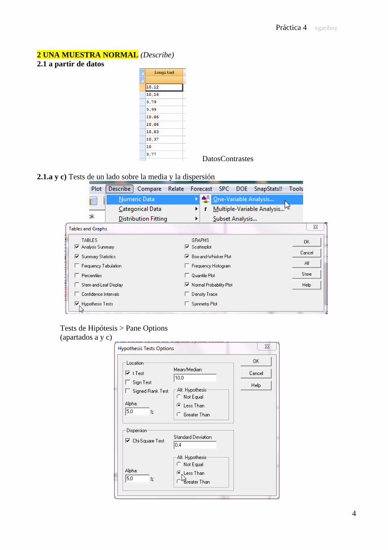
3 DOS Muestras INDEPENDIENTES Normales (Compare) 3.1 A partir de datos 3.1.1 Dos columnas de datos DatosContrastes.sgd TempTipo1 contra TempTipo2 3.1.1 a) Descripción comparada de las dos muestras.

Seleccionar variables y dejar todos los valores por defecto.

Nota: En caso de que los datos se encuentren en una única columna con otra de códigos, los diagramas de cajas se pueden dibujar con Plot/ExploratoryPlots/Box-and-WhiskerPlot/MultipleSamples


10

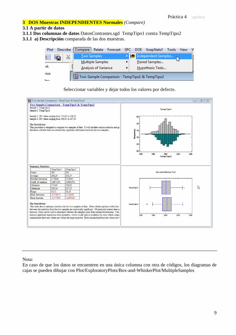
3.1.1 b) Normalidad

Primero una variable, TempTipo1, y luego la otra, TempTipo2


11

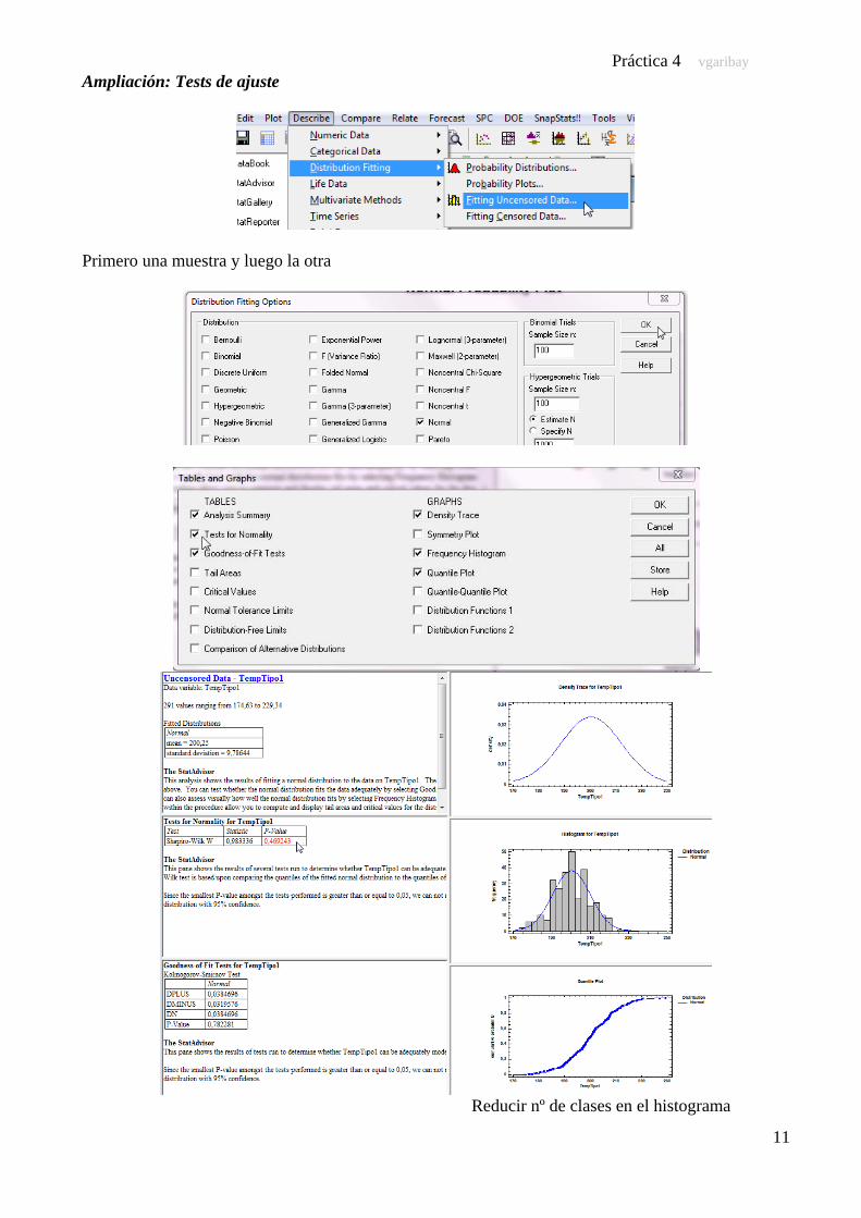
Ampliación: Tests de ajuste

Primero una muestra y luego la otra

Reducir nº de clases en el histograma


12

3.1.1 c) Comparación medias 2 muestras independientes. Ampliamos el apartado 3.1.1.a) incorporando el contrastes de comparación de medias (1 lado), previa comparación de varianzas.

Tests de Hipótesis > Pane Options para indicar , , un lado y sigmas iguales:


13

Salidas de Statgraphics:

F-test to Compare Standard Deviations Null hypothesis: sigma1 = sigma2 Alt. hypothesis: sigma1 NE sigma2 F = 0,956938 P-value = 0,708066 Do not reject the null hypothesis for alpha = 0,05.

t test to compare means Null hypothesis: mean1 = mean2 Alt. hypothesis: mean1 < mean2 assuming equal variances: t = -1,60943 P-value = 0,0540328 Do not reject the null hypothesis for alpha = 0,05.


14

3.1.2 Una columna de datos y otra de códigos que definen los dos grupos Datos robles.sgd

Marcar “Data (Potasio) and Code (Variedad) Columns”

Comparar medias y varianzas

F-test to Compare Standard Deviations Null hypothesis: sigma1 = sigma2 Alt. hypothesis: sigma1 NE sigma2 F = 0,515507 P-value = 0,216385 Do not reject the null hypothesis for alpha = 0,05.

t test to compare means Null hypothesis: mean1 = mean2 Alt. hypothesis: mean1 NE mean2 assuming equal variances: t = 2,34645 P-value = 0,024576 Reject the null hypothesis for alpha = 0,05.


15

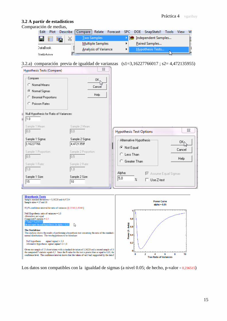
3.2 A partir de estadísticos Comparación de medias,

3.2.a) comparación previa de igualdad de varianzas (s1=3,16227766017 ; s2= 4,472135955)

Los datos son compatibles con la igualdad de sigmas (a nivel 0.05; de hecho, p-valor = 0,236515)


16

3.2.a) comp de medias (dos lados, =0.10, varianzas iguales )

Null Hypothesis: difference between means = 0,0 Alternative: not equal Computed t statistic = 0,197009 P-Value = 0,845551 Do not reject the null hypothesis for alpha = 0,1. (Equal variances assumed).


17

4 DOS Muestras APAREADAS Normales (Compare) A partir de datos (archivo DatosContrastes, dos columnas) H1: mu_sinpin-mu_pin > 0

Pane Options: H1:musinpin-mupin>0

Hypothesis Tests for Sin Pintar - Pintados t-test Null hypothesis: mean = 0 Alternative: greater than Computed t statistic = 5,3936 P-Value = 0,00147879 Reject the null hypothesis for alpha = 0,05.


18

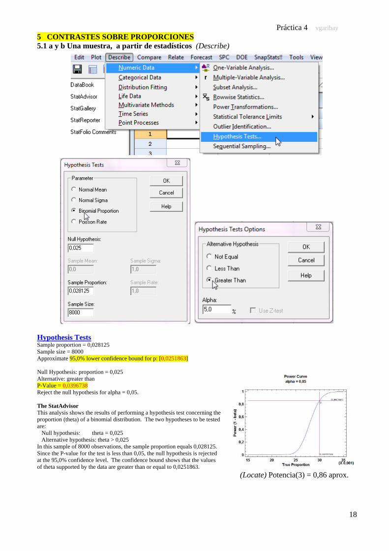
5 CONTRASTES SOBRE PROPORCIONES 5.1 a y b Una muestra, a partir de estadísticos (Describe)

Hypothesis Tests Sample proportion = 0,028125 Sample size = 8000 Approximate 95,0% lower confidence bound for p: [0,0251863] Null Hypothesis: proportion = 0,025 Alternative: greater than P-Value = 0,0396738 Reject the null hypothesis for alpha = 0,05. The StatAdvisor This analysis shows the results of performing a hypothesis test concerning the proportion (theta) of a binomial distribution. The two hypotheses to be tested are: Null hypothesis: theta = 0,025 Alternative hypothesis: theta > 0,025 In this sample of 8000 observations, the sample proportion equals 0,028125. Since the P-value for the test is less than 0,05, the null hypothesis is rejected at the 95,0% confidence level. The confidence bound shows that the values of theta supported by the data are greater than or equal to 0,0251863.

(Locate) Potencia(3) = 0,86 aprox.


19

5.1 c) Tamaño muestral para detectar p=0.03 con prob 0,99

Binomial p, Ho: p=0.025 H1: p>0.025 1 lado, n / (0.03)=0.99 Dif=0.03-0.025 =0.05

Sample-Size Determination Parameter to be estimated: binomial parameter Desired power: 99,0% for proportion = 0,025 versus proportion = 0,03 Type of alternative: greater than Alpha risk: 5,0% The required sample size is n=17114 observations. The StatAdvisor This procedure determines the sample size required when estimating the proportion of a binomial distribution. 17114 observations are required to have a 99,0% chance of rejecting the hypothesis that theta=0,025 when the true theta=0,03 (using a one-sided test).


20

5.2 Dos muestras, a partir de estadísticos (Compare)

Hypothesis Tests Sample proportions = 0,042 and 0,064 Sample sizes = 500 and 500 Approximate 95,0% confidence interval for difference between proportions: [-0,0497375;0,00573753] Null Hypothesis: difference between proportions = 0,0 Alternative: not equal Computed z statistic = -1,55267 P-Value = 0,120501 Do not reject the null hypothesis for alpha = 0,05. Warning: normal approximation may not be appropriate for small sample sizes. The StatAdvisor This analysis shows the results of performing a hypothesis test concerning the difference between the proportions (theta1-theta2) of two samples from binomial distributions. The two hypotheses to be tested are: Null hypothesis: theta1-theta2 = 0,0 Alternative hypothesis: theta1-theta2 <> 0,0 In the first sample of 500 observations, the sample proportion equals 0,042. In the second sample of 500 observations, the sample proportion equals 0,064. Since the P-value for the test is greater than or equal to 0,05, the null hypothesis cannot be rejected at the 95,0% confidence level. The confidence interval shows that the values of theta1-theta2 supported by the data fall between -0,0497375 and 0,00573753. NOTE: this test uses a normal approximation. Because of the small sample sizes, this approximation may not be valid.

Práctica 4 PRÁCTICA 4. CONTRASTE DE HIPOTESISvalentin/ging/materiales_web/practica4_guia.pdf ·...

Documents

Transcript of Práctica 4 PRÁCTICA 4. CONTRASTE DE HIPOTESISvalentin/ging/materiales_web/practica4_guia.pdf ·...