Sociedad Española de Estadística e Investigación Operativa ... · e Investigación Operativa...

Test

Sociedad Española de Estadísticae Investigación Operativa

Volume 13, Number 1. June 2004

Families of Distributions Arising

from Distributions of Order StatisticsM. C. Jones

Department of Statistics,The Open University, United Kingdom.

Sociedad de Estadıstica e Investigacion OperativaTest (2004) Vol. 13, No. 1, pp. 1–43

Sociedad de Estadıstica e Investigacion OperativaTest (2004) Vol. 13, No. 1, pp. 1–43

Families of Distributions Arising

from Distributions of Order StatisticsM. C. Jones∗

Department of Statistics,The Open University, United Kingdom.

Abstract

Consider starting from a symmetric distribution F on < and generating a family ofdistributions from it by employing two parameters whose role is to introduce skew-ness and to vary tail weight. The proposal in this paper is a simple generalisationof the use of the collection of order statistic distributions associated with F for thispurpose; an alternative derivation of this family of distributions is as the result ofapplying the inverse probability integral transformation to the beta distribution.General properties of the proposed family of distributions are explored. It is arguedthat two particular special cases are especially attractive because they appear toprovide the most tractable instances of families with power and exponential tails;these are the skew t distribution and the log F distribution, respectively. Limitedexperience with fitting the distributions to data in their four-parameter form, withlocation and scale parameters added, is described, and hopes for their incorporationinto complex modelling situations expressed. Extensions to the multivariate caseand to <+ are discussed, and links are forged between the distributions underlyingthe skew t and log F distributions and Tadikamalla and Johnson’s LU family.

Key Words: Beta distribution, log F distribution, LU distribution, order statis-tics, probability integral transform, skew t distribution.

AMS subject classification: 60E05, 62E10, 62F99

1 Introduction

In this paper, I seek to provide new (and old) families of univariate con-tinuous distributions from a novel perspective. The distributions of orderstatistics of i.i.d. samples from various underlying distributions are cen-tral to the immense literature on order statistics per se (e.g. Reiss, 1989,

∗Correspondence to: M. C. Jones, Department of Statistics, The Open University,Walton Hall, Milton Keynes, MK7 6AA, U.K. Email: [email protected] .

Received: February 2004; Accepted: February 2004

2 M. C. Jones

Arnold et al., 1992, David and Nagaraja, 2003). Here, I extract these orderstatistic distributions from the order statistics literature, generalise them alittle bit, and suggest the use of this collection of generalised distributionsof order statistics as empirically useful families of distributions in their ownright.

Typically, these families of distributions have four parameters, compris-ing two positive, real, parameters a and b associated with the above mech-anism in addition to location and scale parameters introduced in the usualway. Much of this paper is concerned with distribution theory, exploringthe properties of the new families of distributions and, where appropriate,extolling their virtues; relatively little of the paper is devoted to practicalapplication. However, the main point of this exercise is to provide furtherfamilies of distributions for use in the empirical modelling of data, replac-ing normal distributions and the like, where necessary and appropriate,by wider families of distributions that automatically account for skewnessand/or heavy tail weights in the data. Of course, such distributions can,and should, be incorporated in regression, time series and other more com-plex models, and not just, as later in this paper, in the simplest, one sample,situation.

Let me move quickly to giving you the central idea of the paper. Theingredients of the proposed new general family of continuous distributionsare an existing continuous distribution F with density f together with theparameters a > 0 and b > 0 mentioned above. Let B(·, ·) be the betafunction. Then, I propose consideration of

gF (x; a, b) = {B(a, b)}−1f(x)F a−1(x)(1− F )b−1(x) (1.1)

which is the density of a member of a family of distributions GF indexedby a and b and generated by F . Of course, gF (·; 1, 1) = f(·).

While F could, in general, be quite arbitrary, I propose to concentrateprincipally on cases in which F is symmetric about zero with no free pa-rameters other than location and scale, has support the whole real line andhas tails that are at least as heavy as those of the normal distribution. (Iwill return to consider each of these restrictions briefly later in the paper.)The family GF then affords a class of distributions generated by symmetricF with a and b governing skewness and tail weight: whenever a = b, gF

remains symmetric but with tails getting lighter as a increases and heavieras a decreases; if a 6= b, skewness is introduced, the amount of skewness

Distributions Arising from Distributions of Order Statistics 3

being dependent on the difference between a and b, and its sign on the signof a − b. The reason for taking F to be symmetric should now be clear: Iwish to use a and b alone to control the degree of skewness introduced. Itis easy to see that gF (x; b, a) = gF (−x; a, b).

The genesis of family (1.1) is simple and attractive and is provided,in two closely related ways, in Section 2. As already mentioned, family(1.1) is a generalisation of the distribution of order statistics of a randomsample from F ; this is spelt out in Section 2.1. Family (1.1) is also theresult of applying the inverse probability integral transformation to thebeta distribution; see Section 2.2.

The basic exemplar of family (1.1) is the beta distribution itself whicharises immediately if F is taken to be the uniform distribution. Two furtherspecial cases of (1.1) are particularly tractable and form the major examplesof the general approach in this paper. These are the skew t distribution ofJones (2001b) and Jones and Faddy (2003) — the a = b symmetric membersof this family being the usual Student t distributions — which has heavy,power, tails and the log F distribution of Fisher (1924) which has lighter,exponential, tails. The skew t and log F distributions are introduced inSection 3 and are used as ongoing examples when the general propertiesof members of family (1.1) are considered in Section 4. These propertiesinclude the role of location and scale parameters, the distribution functionGF , moments, modality, tail weight, limiting cases and relationships withother distributions.

It is envisaged that the families of distributions are fitted to data bymaximum likelihood (I am not the right person to explore Bayesian ap-proaches!). Experience to date with this is described and discussed inSection 5.1 and a simple example is given in Section 5.2. Extensions ofthe basic methodology are considered in Section 6. Section 6.1 considersthe multivariate case; a tractable five-parameter model encompassing bothskew t and log F distributions is described in Section 6.2; and in Section 6.3application of the basic idea to nonnegative data is considered. The papercloses with a discussion section, considering various further possible choicesfor f (Section 7.1), and discussing the role of the distributional families ofthis paper — particularly the skew t and log F distributions — in dataanalysis (Section 7.2).

4 M. C. Jones

2 Genesis of family (1.1)

2.1 Order statistic distributions

The distribution of Xi:n, the ith order statistic in a random sample of sizen from distribution F , is well known to have density

n!(i− 1)!(n− i)!

f(x)F i−1(x)(1− F )n−i(x) (2.1)

(Reiss, 1989, Arnold et al., 1992, David and Nagaraja, 2003) where thereciprocal of the normalising constant can also be written as B(i, n+1− i).In Figure 1(a) is plotted the standard logistic density f(x) = (1 + ex)−2ex

and the five distributions arising as the distributions of the order statisticsof a random sample of size n = 5 from the logistic distribution. Thesefive distributions range from the symmetric, i = 3, through the slightlyasymmetric, i = 2, 4, to the reasonably strongly skewed, i = 1, 5. In Figure1(b) is the more comprehensive family of symmetric and skewed densitiesassociated with sample size n = 35.

As the sets of distributions in Figure 1 form limited families of sym-metric and skew distributions associated with the logistic distribution, soI suggest considering a much wider family of symmetric and skew distri-butions associated with any symmetric distribution F by utilising the fullset of order statistic distributions for each and every n, and extending iteven further. Now, formula (2.1) matches precisely with formula (1.1) ifa = i and b = n + 1− i. But I also ‘fill in the gaps’ between order statisticsassociated with integer i, go beyond the most extreme order statistics downtowards a = 0 and up to a = n + 1, and do not stick with a single integervalue of n. All this is achieved by simply allowing ‘i’ and ‘n+1− i’ to takeany real, and not just integer, positive values.

2.2 Transforming the beta distribution

An alternative, but related, motivation for (1.1) comes through the inverseprobability integral transformation X = F−1(U). This is normally appliedto U following the uniform distribution on (0, 1), in which case X hasdistribution F . But on support (0, 1) the beta distributions Beta(a, b) area natural extension of the uniform by dint of two parameters a > 0 and


-6 -5 -4 -3 -2 -1 0 1 2 3 4 5 6

-6 -5 -4 -3 -2 -1 0 1 2 3 4 5 6

Figure 1: The standard logistic density (dashed line) and its ith order statistic

densities, i = 1, ..., n, going from left to right (solid lines) for (a) n = 5, (b) n = 35.

b > 0 which have the roles outlined for the general case in Section 1:a = b = 1 gives the uniform distribution; a = b 6= 1 gives further symmetricdistributions on (0,1) with steadily lighter tails as a > 1 increases andheavier tails as a < 1 decreases; and if a 6= b, skewness is introduced.Application of X = F−1(B) to B ∼ Beta(a, b) is immediately seen to yieldX ∼ GF .

The link between the two motivations is clear in the case of a = i and

6 M. C. Jones

b = n + 1 − i integer since then it is well known that Ui:n = F (Xi:n) hasthe Beta(i, n + 1 − i) distribution (Reiss, 1989, Arnold et al., 1992, Davidand Nagaraja, 2003).

3 Two particular families of form (1.1) on <

3.1 The skew t distribution

The skew t family of distributions was recently introduced by Jones (2001b)and developed in some detail by Jones and Faddy (2003). The densityfunction of the skew t(a, b) distribution can be written

1B(a, b)

√a + b 2a+b−1

(1 +

x√a + b + x2

)a+1/2 (1− x√

a + b + x2

)b+1/2

,

x ∈ <, a > 0, b > 0. When a = b, the skew t reduces to the usual symmetricStudent’s t distribution on 2a degrees of freedom. Otherwise, a 6= b allowsskewness.

Jones (2001b) and Jones and Faddy (2003) derive the skew t distributionas the distribution of T =

√a + b (2B−1)/{2

√B(1−B)} ≡ F−1

T (B) whereB ∼ Beta(a, b). Here, we recognise that

FT (t) =12

(1 +

t√a + b + t2

)

is the distribution function of the scaled Student t distribution on 2 degreesof freedom, with scaling factor

√(a + b)/2, and so the skew t family is the

special case of family (1.1) based on the t2 distribution as F . This impliesthat the skew t(a, b) distributions are the distributions of the order statisticsof the t2 distribution when a and b are integers. I have argued elsewherethat the t2 distribution is itself an unjustly ignored but rather useful simplesymmetric distribution on the real line (Jones, 2002d).

3.2 The log F distribution

Let f be the density of the standard logistic distribution. Then, it is easyto show that

gF (x) =1

B(a, b)eax

(1 + ex)a+b. (3.1)


This is actually the density of X = log(C1/C2) where C1 ∼ χ22a inde-

pendently of C2 ∼ χ22b. Family (3.1) is thus essentially the same family

as that of log F = log(bC1/(aC2)) (Fisher, 1924), the distributions of thelogs of random variables following the F distribution. (Alternatively, thedistribution of log F could be obtained directly from the modified logisticdistribution with f(x) = abex/(b+aex)2, the density of the logistic randomvariable plus log(b/a).) The symmetric members of family (3.1) are ‘TypeIII’ generalised logistic distributions (Johnson et al., 1995, Chapter 23); seealso Smyth (1994).

Important papers on the distribution theory of the log F distributioninclude Aroian (1941) and Barndorff-Nielsen et al. (1982) and on the theoryof fitting the log F distribution to data, Prentice (1975). The log F distribu-tion crops up from time to time over the years, though often under differentnames such as Fisher’s Z distribution, the generalised F distribution and‘Type IV’ generalised logistic distributions. Brown et al. (2002) recentlymade a bid to (re-)popularise the log F distribution as a useful tool forpractice. It also appears, but with none of the names above, as conjugateprior density for the regression parameter in logistic regression (Greenland,2001). The fact that the log F distribution, for even integer parameters,is the distribution of the order statistics from the logistic distribution isknown (e.g. Birnbaum and Dudman, 1963), but is rarely mentioned in theliterature. The densities in Figure 1 are, consequently, log F densities.

4 Properties of family (1.1)

General properties of family (1.1) are available as analogues and extensionsof results for order statistic distributions (Reiss, 1989, Arnold et al., 1992,David and Nagaraja, 2003). For empirical purposes, however, family (1.1)is a standard form which requires the addition of extra location and scaleparameters; see Section 4.1 and Section 5. After Section 4.1, we revert tothe standard form (1.1) for the remainder of this section.

8 M. C. Jones

4.1 Location and scale parameters

For fitting a family GF to data, it is natural to replace (1.1) by its fourparameter form

1σ

gF

(x− µ

σ; a, b

)=

1B(a, b)σ

f

(x− µ

σ

)F a−1

(x− µ

σ

)(1− F )b−1

(x− µ

σ

). (4.1)

Notice that µ and σ are modifications to location and scale in the sensethat if Z follows the density in standard form and T follows density (4.1),E(T ) = µ+σµG, Var(T ) = σ2σ2

G where µG = E(Z) and σ2G = Var(Z). This

is particularly important to bear in mind in regression, where the obviousmodel Y = XB+ε with ε ∼ gF (·/σ)/σ corresponds to E(Y |X) = XB+σµG

and Var(Y |X) = σ2σ2G.

Notice that, in general, a relocation and/or rescaling of f translatesdirectly to the same relocation and/or rescaling of gF : σ−1f(σ−1(x − µ))and F (σ−1(x − µ)) in density (1.1) yield density (4.1). So, in the skew tcase, if readers object to the introduction of the

√(a + b)/2 scaling into

f they can think of it as a rescaling of gF instead. In the log F case, thelocation role of log(b/a) is covered by this.

4.2 Distribution function

Immediately from the transformation motivation, the distribution functionis

GF (x) = IF (x)(a, b),

where Iu(·, ·) is the incomplete beta function ratio, the distribution functionof the beta distribution with parameters a and b.

It may be interesting to note that some expansions of GF (x) from theorder statistics literature, for example

GF (x) =b−1∑

r=0

(a + b− 1

r

)F a+b−r−1(x)(1− F )r(x)

and

GF (x) = 1−a−1∑

r=0

(a + b− 1

r

)F r(x)(1− F )a+b−r−1(x),


continue to hold if just the appropriate one of a or b are integer with theother parameter allowed to be real, provided the combination terms areinterpreted in terms of gamma functions. This partial generalisation of(2.1) in the direction of (1.1) was considered by Rohatgi and Saleh (1988).

4.3 Moments

The usual integral formula for E(Xr) for X ∼ gF is, of course, equal tothat for E{(F−1(B))r} for B ∼ Beta(a, b) and is written out for the orderstatistic case a = i, b = n − i + 1 on p.22 of Arnold et al. (1992). Therth moment is also the {r, a − 1, b − 1}th probability weighted moment(Greenwood et al., 1979) of f . Whether or not the moments are tractableis a question to be answered on a case by case basis. As they often arenot, extensions of asymptotic formulae and bounds for the moments oforder statistics will be relevant (Reiss, 1989, Arnold et al., 1992, David andNagaraja, 2003). Because of the integer nature of i and n there is alsoa lot of work in the order statistics literature on recurrence relations formoments; these may not be of such interest in the general case.

The moments of both the skew t and log F families are tractable whenthey exist. Jones and Faddy (2003) give the moments of the former; thesemust, of course, take the same form as the moments of the order statisticsfrom the t2 distribution. Jones and Faddy’s formulae show that Vaughan’s(1992) formulae for the mean and variance of the latter are far more com-plicated than they need to be (Jones, 2002d). Likewise, the moments of thelog F distribution must take the same form as the moments of the orderstatistics from the logistic distribution. The moment generating functionis particularly simple in both cases; compare Aroian’s (1941) formula forthe former with Gupta and Shah’s (1965) formula for the latter.

4.4 Modality

Let f be unimodal and continuously differentiable; if a = b ≥ 1, it isstraightforward to show that gF is also unimodal. However, it is not thecase that unimodality of f translates to unimodality of gF generally. Workon the unimodality of order statistic distributions translates directly tothe current situation when a, b > 1 because it does not depend on a andb being integer. See Reiss (1989, pp. 48–49) for a fine summary. One

10 M. C. Jones

result is that strong unimodality, i.e. log concavity, of f implies strongunimodality of gF (Barlow and Proschan, 1966, Theorem 7.2). This coverse.g. uniform, logistic and normal f ’s. A slight extension to the case of f ′/f2

nonincreasing also affords unimodality of gF and allows t distributions asf as well.

I have no general result if a < 1 and/or b < 1. Indeed, strange thingscan happen in some cases! For example, when a < 1 and b < 1, thebeta distribution, which is gF for the uniform’s f , has modes replaced byantimodes. Away from the finite support that causes the beta distribution’sbehaviour, Eugene (2001) apparently considered the normal-based versionof (1.1) and observed bimodality for a region of values of a and b both lessthan 0.214; see Eugene et al. (2002). However, Aroian (1941) and Jones andFaddy (2003) observe that the log F and skew t distributions, respectively,are unimodal for all a, b > 0.

4.5 Tail weight

It is straightforward to see the effect of formula (1.1) on tail weight fordistributions with infinite support. Consider the right-hand tail, x → ∞,for which F (x) → 1. Typically, right-hand tail weight is monotonic in b: asb increases, tail weight decreases, as b decreases, tail weight increases.

If f has power tails, f ∼ x−(α+1), α > 0, for large x, then the tails ofgF go as gF ∼ x−bα−1. In this case, tail weight increases towards the veryheavy limit of x−1 as b approaches 0, regardless of the value of α. The skewt distribution is in this class with α = 2.

If f has exponential tails, f ∼ e−βx, β > 0, then gF ∼ e−bβx. Theexponential nature of the tails remains for all b. The log F distribution isin this class.

Finally, if f has normal tails, f ∼ e−x2/2, 1 − F ∼ f/x (e.g. Patel andRead, 1982, Chapter 3) and so gF ∼ e−bx2/2/xb−1.

For the left-hand tail, x → −∞, the above arguments should be modi-fied by replacing x by |x| and b by a.

It can, therefore, be argued that a and b introduce skewness into gF inthe following way: a and b directly control the relative weights of the left-and right-hand tails of the distribution, respectively, so if a 6= b, skewness


arises as a ‘secondary’ consequence of having differently weighted tails.

4.6 Limiting distributions

Aroian (1941), in the log F case, and Jones and Faddy (2003), in the skewt case, note that if a and b both tend to ∞ in essentially any manner,then gF becomes normal. This can now be seen as the direct analogueof the normal limiting behaviour of both central, i.e. a/b → c, a non-zeroconstant, and intermediate, i.e. a/b or b/a → ∞, order statistic densitieswhere both parameters tend to ∞ (Arnold et al., 1992, Section 8.5, Reiss,1989, Section 4.1). Indeed, a proof for order statistics such as that inReiss (1989) doesn’t depend on a or b being integer and hence extendsimmediately to asymptotic normality in the present case as a, b → ∞ forany version of (1.1) provided f is continuous and positive.

Now, fix b but let a →∞. If b is an integer, the limiting distribution isprecisely that of the bth largest order statistic (Arnold et al., 1992, Section8.4, Reiss, 1989, Section 5.1). For a distribution with power tails, likethe t2/skew t, the limiting density is proportional to x−(αb+1) exp(−x−α),x > 0, the Frechet form of extreme value distribution when b = 1; for anyb > 0, this limiting distribution is the distribution of E

−1/αb where Eb follows

the gamma distribution with parameters b and 1. For a distribution withexponential tails, like the logistic/log F , the limiting density is proportionalto e−bx exp(−e−x), x ∈ <, the Gumbel form of extreme value distributionwhen b = 1; for any b > 0, this limiting distribution is the distributionof − log Eb. It would appear that these limiting distributions continue tohold for any b ≥ 1. This is essentially confirmed for the skew t distribution,which has α = 2 and hence an inverse chi limiting case, by Jones and Faddy(2003).

Heuristic calculations, not given, suggest that these results can alsobe extended to cover all b > 0 with appropriate choice of normalisingconstants.

4.7 Distributional relationships

Generation of random variates with distribution (1.1) proceeds most eas-ily from the relationship in Section 2.2: X = F−1(B) ∼ GF where B ∼

12 M. C. Jones

Beta(a, b). This is because of the existence of fast generators for beta ran-dom variables e.g. Devroye (1986, Section IX.4).

Since B has the same distribution as Wa/(Wa + Wb) where Wa ∼ χ22a

and Wb ∼ χ22b, independently, and equivalently aF/(b + aF ) where F ∼

F (2a, 2b), relationships of (1.1) with a pair of independent χ2 distributionsand with the F distribution are immediate.

5 Fitting family (4.1) to data

5.1 Fitting family (4.1) by likelihood

It is natural to fit order statistic distributions in the form (4.1) to data bymaximum likelihood. My general strategy in fitting order statistic distri-butions often starts with something that has not been discussed yet! InSection 6.2, a five-parameter distribution is described which encompassesboth skew t and log F distributions; the maximum likelihood estimatorof the extra parameter can serve as a guide to (the weight of tails in thedata and therefore) which of the skew t or log F distributions is to be pre-ferred. Likelihood ratio tests are available to test the appropriateness ofvarious sub-models of the general model, these, of course, providing appeal-ing simplifications in practice. Overall, discrimination between sub-modelsincludes the choice between skew t and log F models, the appropriatenesson occasion of limiting extreme value-type distributions and, of course, thenormal and, rather importantly, testing for symmetry, a = b, of the dis-tribution fitted to data. One can also estimate and test values of locationand/or scale in the same framework. And one can, of course, go on to in-troduce covariates into the location term in a regression context, et cetera,et cetera.

Both log F and skew t distributions have recently been applied to datausing maximum likelihood. Renewed interest in the log F distribution isparticularly displayed in Brown et al. (2002) who describe a number of ap-plications as well as discussing computational issues. Recent examples ofthe incorporation of the log F distribution into complex statistical modelscan be found in Peng et al. (1998) and Huillard d’Aignaux et al. (2003).Two examples of the application of the skew t distribution have been pub-lished in Jones and Faddy (2003). In addition, Jones and Larsen (2004)successfully fit skew t and log F distributions — preferring log F — to


daily temperature data in the bivariate case.

It proves useful to utilise the following reparametrisation of a and b dueto Prentice (1975):

p =2

a + b, q =

a− b√ab(a + b)

.

Prentice introduced this reparametrisation for the log F distribution “toinduce regular estimation on the boundary with one or both (of a and b)infinite.” Jones and Faddy (2003) showed that the same parametrisationhas the same regularisation effect in the skew t distribution, and it is nat-ural to conjecture that the same is true more widely, but this has not beenproved. However, Jones and Faddy’s further take on this reparametrisa-tion is that, in practice, it appears to make for better behaved likelihoodsurfaces, behaving like a partial orthogonalisation of parameters, if you will.

The author’s practical experience with these models is, as yet, lim-ited. Likelihood estimation seems, empirically, to be fairly well-behavedin as much as implementation using NAG (Numerical Algorithms Group,2003) optimisation routines normally gives sensible and consistent answersthat remain the same when re-run from different starting points. (Occa-sional difficulties arise, mostly when a parameter seeks its limiting value,but statistical common sense usually makes clear what is going on.) Thatsaid, a full and detailed study on the performance of maximum likelihoodestimation for these models, involving simulations and further theoreticalcalculations, would be valuable and remains to be done.

5.2 Example

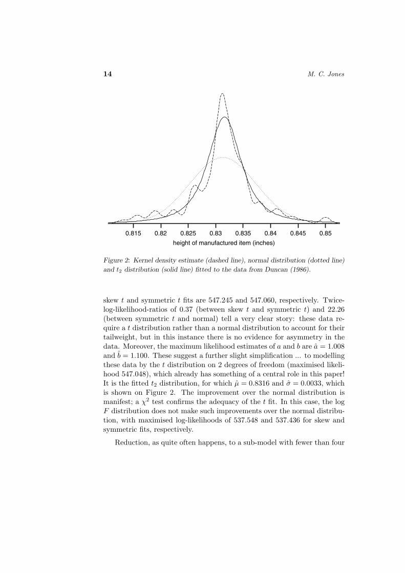
Here is a simple example. The data, with n = 145, can be found in Table3.2 of Duncan (1986) and arise from a 1945 report of L.A. Kauffman onthe results of a manufacturing process (heights, in inches). The data areutilised by Duncan as an example of the normal distribution of variabilityin manufacture. However, the histogram of the data given as Figure 3.2 ofDuncan (1986) and the kernel density estimate in Figure 2 (using Sheather-Jones bandwidth; Wand and Jones, 1995) clearly indicate heavier thannormal tails.

The value of the maximised log-likelihood for fitting the normal dis-tribution to Duncan’s data is 535.928. The corresponding values for the

14 M. C. Jones

0.815 0.82 0.825 0.83 0.835 0.84 0.845 0.85

height of manufactured item (inches)

Figure 2: Kernel density estimate (dashed line), normal distribution (dotted line)

and t2 distribution (solid line) fitted to the data from Duncan (1986).

skew t and symmetric t fits are 547.245 and 547.060, respectively. Twice-log-likelihood-ratios of 0.37 (between skew t and symmetric t) and 22.26(between symmetric t and normal) tell a very clear story: these data re-quire a t distribution rather than a normal distribution to account for theirtailweight, but in this instance there is no evidence for asymmetry in thedata. Moreover, the maximum likelihood estimates of a and b are a = 1.008and b = 1.100. These suggest a further slight simplification ... to modellingthese data by the t distribution on 2 degrees of freedom (maximised likeli-hood 547.048), which already has something of a central role in this paper!It is the fitted t2 distribution, for which µ = 0.8316 and σ = 0.0033, whichis shown on Figure 2. The improvement over the normal distribution ismanifest; a χ2 test confirms the adequacy of the t fit. In this case, the logF distribution does not make such improvements over the normal distribu-tion, with maximised log-likelihoods of 537.548 and 537.436 for skew andsymmetric fits, respectively.

Reduction, as quite often happens, to a sub-model with fewer than four


parameters does not, in one sense, illustrate full use of the full model. Thereagain, the full model is extremely valuable here, and elsewhere, in providingstrong and ready evidence of the appropriateness of the sub-model.

6 Extensions

6.1 Multivariate generalisations

Perhaps the most obvious multivariate generalisation of (1.1) comes fromgeneralising (2.1) to the joint distribution of several order statistics. Thesame result can be obtained by applying the probability integral transfor-mation in an appropriate way to the Dirichlet distribution. There is anunusual sample space associated with this, namely x1 < x2 < ... < xd,where d denotes dimensionality. However, there seem to be many practi-cal situations where such ordered data arise but in such a way that themechanism underlying the data is not readily modelled. In such cases, useof generalised joint order statistic distributions is an attractive empiricaloption. For full details and an interesting application, see Jones and Larsen(2004).

The easiest way to build multivariate models on the whole of <d re-lated to univariate generalised distributions of order statistics would seemto be to consider general linear transformations of a set of d independentunivariate generalised distributions of order statistics, an approach recentlypropounded (with different univariate components) by Ferreira and Steel(2003). Note, however, that the marginal distributions of the original vari-ables will not themselves be generalised order statistic distributions.

Multivariate extensions somewhat akin to Azzalini and Dalla Valle’s(1996) multivariate skew normal distribution might be obtained by intro-ducing a single marginal distribution of form (1.1) to a multivariate spher-ically symmetric distribution generated by F using the simple device ofmultiplicative marginal replacement; see Jones (2002a). It is also possibleto utilise the representation B = Wa/(Wa +Wb) to generate a fairly highlycorrelated multivariate distribution with marginals of the form (1.1) withparameters ai, b, i = 1, ..., d by writing Bi = Wai/(Wai + Wb) with the W ’sindependent except for Wb being common to all Bis. In the logistic casethis provides the logged version of the multivariate F distribution in John-son and Kotz (1972, Chapter 40, Section 8). The uniform case provides a

16 M. C. Jones

novel multivariate beta distribution and the t2 case provides a multivari-ate skew t distribution, both considered by Jones (2001a); the multivariatebeta distribution has since been reinvented by Olkin and Liu (2003).

6.2 Families covering the t2 and logistic, and hence skew t andlog F distributions

Let Y = U/(1−U) where U is a uniform random variable on (0, 1), so that Yfollows the F distribution on 2 and 2 degrees of freedom. Then Z0 = log Yhas the standard logistic distribution and Z1/2 =

√Y −

√1/Y =

√2T2

where T2 has the t distribution on 2 degrees of freedom. Noting that Z0 =(log Y − log(1/Y ))/2, these are the k = 0 and k = 1/2 special cases of

Zk =12k

(Y k − 1

Y k

), (6.1)

provided the k = 0 special case is defined by continuity. The family ofdistributions of Zk, k ≥ 0, is a family of symmetric distributions on < withdensity function

fk(z) =

(kz +

√k2z2 + 1

)1/k

√k2z2 + 1{1 + (kz +

√k2z2 + 1)1/k}2

,

whose k = 0 and k = 1/2 special cases are the logistic and (scaled) t2distributions, respectively. Its distribution function is

Fk(z) =

(kz +

√k2z2 + 1

)1/k

1 + (kz +√

k2z2 + 1)1/k.

It turns out that these distributions are nothing other than scaled ver-sions of the symmetric special cases of Tadikamalla and Johnson’s (1982)LU distributions. The symmetric LU distributions are defined by Lk =sinh(kZ0) where Z0, as above, follows the standard logistic distributionand k = 1/δ in Tadikamalla and Johnson’s notation. Then Zk has the dis-tribution of Lk/k = sinh(kZ0)/k which is readily seen to equate to (6.1).Notice that as z → ∞, fk(z) ∼ z−((1/k)+1). It follows that the family ofsymmetric LU distributions acts as an analogue of the family of Studentt distributions: 1/k is the analogue of the usual degrees of freedom pa-rameter ν controlling the power-of-z tail weight, and hence existence of


moments, with the logistic distribution usurping the position of the normaldistribution as the limiting case of the family (as k → 0, ν → ∞). It hasnot been previously recognised that the t2 distribution is a member of theLU family. Of course, the full LU family of distributions incorporates afurther parameter that introduces and controls skewness and is, in a sense,a four-parameter competitor to the skew t distributions, although one notincorporating the normal distribution. The LU family also has other attrac-tive characteristics such as a simple quantile function and L-moments; a lessattractive characteristic is that the amount of skewness is not monotonicin the skewness parameter.

The five-parameter family encompassing both skew t and log F distri-butions, promised in Section 5.1, follows as the order statistic distributionassociated with Fk. It, immediately, has density

g(z; a, b, k) =

(kz +

√k2z2 + 1

)a/k

B(a, b)√

k2z2 + 1{1 + (kz +√

k2z2 + 1)1/k}a+b. (6.2)

Again, k = 1/2 yields the (scaled) skew t distribution, k = 0 the log F ;the distributions can also be viewed as those of sinh(k log F )/k where log Ffollows the log F distribution. This too affords considerable tractability,but as I currently view the use of a fifth parameter in families of distribu-tions with some disdain and include it only as a sometimes useful device inpractice, the general properties of family (6.2) will not be explored here.

An alternative family of distributions including both logistic and t2distributions is those whose density function f and distribution function Fsatisfy the relationship f(x) ∝ {F (x)(1− F (x))}c; the logistic distributioncorresponds to c = 1, the t2 to c = 3/2. This family of distributions isalso interesting (Kamps, 1991, Jones, 2002b, Balakrishnan and Akhundov,2003) but is less tractable than the above.

6.3 Order statistic distributions on <+

The idea remains to generalise the family of distributions of order statisticsby taking parameters a, b > 0 to be real-valued rather than integer. Butnow the starting point is a distribution F+ with — in imitation of the‘canonical’ situation on the whole real line — a monotone non-increasing

18 M. C. Jones

density f+, with no free parameters except scale, on the positive half line.The basic proposal is therefore to consider gF+(x; a, b) in (1.1).

Without loss of generality, F+ could be thought of as the truncation to<+ of a distribution F symmetric about zero on < or, equivalently, as thedistribution of |Z| when Z ∼ F . In this case, for x > 0, f+(x) = 2f(x) andF+(x) = 2F (x)− 1 leading to

gF+(x; a, b) = {B(a, b)}−12a+b−1f(x)(F − 1/2)a−1(x)(1− F )b−1(x) (6.3)

and GF+(x; a, b) = I2F (x)−1(a, b). It also follows that if X+ ∼ GF+(·; a, b)and B ∼ Beta(a, b) on [0, 1] as before, then X+ has the same distributionas F−1 ((B + 1)/2).

What are the principal effects of a and b in this case? Well, it should beclear that b has precisely the same effect on the right-hand tail of the distri-bution, in conjunction with f , as it does in the case of the whole real line.This is attractive when compared, for example, to transformations from <which have the capacity to alter right-hand tail behaviour drastically.

The parameter a, meanwhile, shifts its attention to behaviour of gF+

near the origin, and it does this in a very appealing way too provided it isassumed that, as is usually but not always the case, f(0) is finite. Then, aTaylor series expansion of density (6.3) shows that, as x → 0,

gF+(x) ' {B(a, b)}−1{2f(0)}axa−1.

So, provided f(0) < ∞, gF+(x) always behaves as xa−1 as x → 0. Thisis an attractive property shared with many popular distributions on thepositive half line (e.g. gamma, Weibull) implying that members of family(6.3) exhibit densities at the origin that drop to zero if a > 1, are finite ifa = 1 and have a pole if 0 < a < 1.

In the following subsections, I look briefly at two distributions that formanalogues of the log F and skew t distributions on <+ in the sense of beingtractable and having exponential and power right-hand tails, respectively.Note that these do not arise from the half-logistic or half-t2 distributions;one could look at the distributions corresponding to these, but their or-der statistics happen not to provide such a great deal of tractability astheir equivalents do on <. Both families of distributions proposed are pre-existing, but do not seem to have much of a role in survival or reliabilityanalysis; I wonder if they should do?


6.3.1 Exponential F+; log(beta) GF+

Exponential F+ clearly gives rise to the distribution of minus the log of abeta random variable with parameters b and a on [0,1]:

gF+(x; a, b) = {B(a, b)}−1(1− e−x)a−1e−bx. (6.4)

These densities (necessarily) behave like xa−1 near the origin and are pro-portional to e−bx as x →∞.

The monotonicity of the failure rate of this family of distributions de-pends only on a: the log beta distribution has increasing failure rate (IFR)if a > 1, is the exponential distribution with constant failure rate for a = 1,and has decreasing failure rate (DFR) if 0 < a < 1. These claims for a 6= 1can readily be demonstrated by application of Lemmas 5.8 and 5.9 of Bar-low and Proschan (1975) which notes the connection between monotonicityof failure rate and log-concavity/convexity of the density function. In fact,(log gF+)′′(x) = −(a− 1)e−x < (>)0 as a > (<)1 and the result follows.

It seems to me to be unusual for the failure rate properties of a familyof distributions with two shape parameters to be so simple and to dependon only one of them. This could be an attractive property of log(beta)distributions as a family of lifetime distributions, and yet they are barelymentioned in Johnson et al. (1995) except for the provision of their cu-mulants (p.218). It might, however, be argued that the above makes brelatively unimportant. The subset of family (6.4) with b = 1 (the distri-bution of the generalised maxima of independent exponentials, or equiv-alently of − log(1 − U1/a) where U is uniform on [0, 1]) has recently seenmuch attention under the names ‘generalized exponential distribution’ and‘exponentiated exponential distribution’ in a series of papers by Gupta andKundu (1999, 2001a,b, 2003a,b).

6.3.2 F2,2 F+; general F GF+

My favourite simple example of a heavy-tailed distribution in this contextis simply the well-known F distribution (e.g. Johnson et al., 1995, Chapter27). The F distribution on 2a and 2b degrees of freedom, F2a,2b, arises asGF+ to the F2,2 distribution which was also involved in Section 6.2 andwhich has simple density f(x) = 1/(1 + x)2. (That is, I generalise the fact

20 M. C. Jones

that the order statistics from the F2,2 distribution follow F distributionson even integer degrees of freedom, specifically F2i,2(n+1−i).)

In olden days, F distributions, like t distributions were of interest almostwholly because of their link to normality as sampling distributions. Thishas changed for the t distribution in recent years, with it now often beingused as an empirical model with heavy tails to inculcate robustness (e.g.Lange et al., 1989). Might there not be a similar empirical, robustifying,role for the F distribution in survival or reliability analysis?

7 7 Discussion

7.1 More on choices of f on <

Further special cases of (1.1) readily present themselves as being of potentialinterest. A very natural choice for f would be the normal density φ (withdistribution function Φ); gΦ has recently been discussed by Eugene et al.(2002). Earlier, the generalised distribution of the maximum, gΦ(x; a, 1) =aφ(x)Φa−1(x), was considered by Durrans (1992) and is a direct competitorto the ‘skew-normal distribution’ 2φ(x)Φ(λx) with λ > 0 (Azzalini, 1985).But, of course, distribution (1.1) with f = φ offers much more flexibilityin general through its two parameters. However, the normal-based versionof (1.1) is not particularly tractable, as the wealth of literature on normalorder statistics makes plain. There again, there is much such material,albeit largely approximate, to draw on. It could well be, however, that theneed for allowing normality as a special case of (1.1) is better served byutilising its position as limiting case of (1.1) for a, b → ∞ and choosing adifferent f which allows departures from normality of a more flexible kind.

It is tempting to suggest setting f to be the Cauchy density in (1.1) toprovide a direct competitor to the stable laws (Samorodnitsky and Taqqu,1994) as a family of very heavy-tailed distributions including skewed ver-sions. This g and the stable laws have normality as a limiting special caseand, in appropriate senses, the Cauchy as a ‘central’ special case. But ghas an explicit tractable form which the stable densities do not; conversely,the stable distributions have other attractive properties that ‘gcauchy’ doesnot. That said, the skew t family also includes the Cauchy distribution,a = b = 1/2, and other even heavier-tailed distributions, a, b < 1/2, and socan play a similar role in a more tractable way.


The Laplace or double exponential density can act as f in (1.1) anddoes afford considerable tractability. However, unsurprisingly, its lack ofdifferentiability at zero is inherited by all members of family (1.1). Johnsonand Kotz (1973) and Ratnaparkhi and Mosimann (1990) investigate theresult of taking X = F−1(B) when F−1 corresponds to the symmetricTukey lambda distribution.

What of families of lighter-tailed distributions on <? The exponentialpower distribution (e.g. Box and Tiao, 1973, Tadikamalla, 1980) with powergreater than 2 might provide an interesting generating function. In par-ticular, the fourth power density, f(x) = {2Γ(5/4)}−1 exp(−x4), might beespecially interesting, as suggested to me by Malcolm Faddy. Two relatedworries arise. The first is that, as for all generating f with lighter-than-normal tails, tail weight will increase both for a, b decreasing, as before,and for a, b increasing, as the distributions tend towards normality. Onetherefore specifies by choice of f the lightest tail weights in the family.(In a rough sense, generalised distributions of order statistics have at least‘min(f, φ)-tails’.) The second is that what I would call an arbitrary, uncon-trolled, bimodality appears for small a, b, as observed by Eugene for normalf .

7.2 So, might this work be useful?

I hope so! Incorporation of four-parameter families of distributions forrandom quantities in modelling exercises automatically allows for the effectsof skewness and (heavy) tail weights. Of course, for small to moderatesample sizes, there will typically be insufficient information in the data toestimate the parameters a and b well (very large sample sizes will normallybe necessary for that). But also this will not usually be very important.Interest would normally be in location and perhaps scale parameters and,typically, in further parameters involved in incorporating covariates intothese. A burgeoning area in which distributions somewhat analogous tothe skew t are already proving useful as parts of more complex models isfinancial and economic time series analysis (e.g. Rydberg, 2000). If one canonly reliably discriminate between some of the more extreme members ofthe families of generalised distributions of order statistics (f itself, normal,extreme value-type distributions, much heavier tails) then one can stillaccount for the main part of the influences of skewness and/or heavy tails.

22 M. C. Jones

I should add that family (1.1) should also be very useful in investigationsof procedures based on symmetric/normal distributions in order to studyrobustness to departures from assumptions.

Finally, I reiterate that it seems to me that the two distributions chosenas illustrative special cases throughout this paper, the new skew t distri-bution and the old log F distribution, have a special role to play. Thekeys are their extensive level of tractability and their tail weights. Theskew t and log F distributions are tractable representatives of family (1.1)with heavy, power, tails and lighter, exponential, tails, respectively. Manyother special cases of (1.1) on < will directly compete with one or other ofthese depending on tail behaviour and yet apparently lack the same levelof tractability.

Acknowledgements

I am very grateful to Elja Arjas, Gopal Basak, Frank Critchley, MalcolmFaddy and Pia Larsen for their helpful comments on this work and toRolf-Dieter Reiss for alerting me to the literature on unimodality of orderstatistic distributions.


DISCUSSION

Barry C. ArnoldUniversity of California

Riverside, USA

Professor Jones has provided us with an entertaining survey of densitiesobtainable by applying the probability integral transformation or if youwish the quantile function of F to a Beta (a, b) random variable instead ofa uniform (0, 1) random variable. In this manner a two parameter family ofdistributions is obtained containing the “parent” distribution F as a specialcase (corresponding to a = 1, b = 1)

gF (x; a, b) = {B(a, b)}−1[F (x)]a−1[1− F (x)]b−1f(x) . (1)

The family of densities (1) will be most tractable when the parent dis-tribution and its corresponding density have simple analytic forms. Ashe observes, the logistic distribution and the t distribution with two de-grees of freedom are good examples with the real line as support. An-other example is the Cauchy distribution. Distributions on (0,∞) withboth density and distribution functions of simple form include the Weibulland Pareto distributions. On a finite support set such as (0, 1), we mightconsider a parent distribution of the form F (x) = xδ, 0 < x < 1 orF (x) = 1− (1− x)δ, 0 < x < 1.

Except for these well behaved choices for F in (1), it would appearthat the model will be difficult to deal with. Nevertheless, it is good tohave it available. Its appeal would be considerably enhanced if we couldenvision some kind of stochastic mechanism which would naturally lead toobservations from (1) beginning perhaps with observations from the parentdistribution F . Such a mechanism is of course available when a and b arepositive integers in terms of order statistics. What we need is a stochasticscenario leading in some way to fractional order statistics. Is a viablemechanism of this type well known?

24 Barry C. Arnold

The submodel of (1) in the spirit of Durrans (1992), i.e. gF (x; a, 1) =aF a−1(x)f(x), has been discussed in a variety of settings under the labelof Lehmann alternatives. It is perhaps interesting to observe that if theparent density f is chosen to be a member of a max-stable family, then theresulting densities of the form gF (x; a, 1) will again be in that max-stablefamily so that, in this instance, there is no gain in generality encountered.A parallel statement can be given if we consider gF (x; 1, b) and a min-stableparent density f .

A family of densities closely related to Durran’s model was introducedby Balakrishnan (2002). It was, in a sense, more general than Durran’smodel, since a skewness parameter was introduced. It was more restrictive,in the sense that a was assumed to be an integer. Arnold and Beaver (2002)suggested removal of the integer restriction and the introduction of a secondskewness parameter, thus arriving at a family of models of the form

f(x; λ0, λ1, α) ∝ [Φ(λ0 + λ1x)]a−1ϕ(x) ,

where ϕ and Φ would denote the standard normal density and distributionfunction respectively.

In the spirit of the current paper it is natural to replace Φ by a generalparent distribution F , and moreover to relax the constraint that b = 1.We thus arrive at the skewed generalized order statistic distribution of theform

gF (x; a, b, λ0, λ1) ∝ (F (λ0 + λ1x))a−1[1− F (λ0 + λ1x)]b−1f(x) (2)

where λ0, λ1 ∈ < and a, b ∈ <+.

The chief virtue of such a four parameter family is not that it would betypically used to model data, since estimation of the four parameters wouldundoubtedly be challenging. Its virtue lies in the fact that it includes asspecial cases many models already introduced in the literature. For (2) tobe useful we would need some plausible approach to the problem of testingsimplifying hypotheses, such as, for example, λ0 = 0 or λ1 = 1 or a = 1,etc.

Having introduced (2) and observed its overabundance of parameters,it is perhaps not wise to suggest an even more general model. Risking, achorus of hisses, we could consider a generalized version of the Arnold andBeaver (2000) multiple-constraint skewed model. In this fashion we will


arrive at the class of densities of the form

gF

(x; a, b, λ(0), λ(1)δ(0), δ(1)

)∝

k∏

j=1

[F (λ(0)

j + λ(1)j x)

]aj−1

×m∏

`=1

[1− F (δ(0)

j + δ(1)j x)

]bj−1f(x)(3)

where λ(0), λ(1) ∈ <k, a ∈ <+k, δ(0), δ(1) ∈ <` and b ∈ <+`. This typeset-ters’ nightmare makes a good stopping point. Conceivably model (2) maybe useful. Model (3) in full generality is surely not but, could it be thatsome form intermediate between (2) and (3) might find a niche for itself.

For all of the flexible models described above, the inevitable call willbe for more work on problems related to parameter estimation, hypothesistesting and model fitting. I am sure that Professor Jones deftly fashionedintroduction to such models will prove to be a siren call to researchers anda rich harvest of follow-up articles can be confidently envisioned.

H. A. DavidDepartment of Statistics

Iowa State University, U.S.A.

This is an impressive paper, covering much ground and making manyinteresting connections between very different distributions. The main ideais to generalize the distribution of the ith order statistic in a random samplefrom f(x), namely

1B(i, n− i + 1)

f(x)F i−1(x) [1− F (x)]n−i

in order to generate various families of distributions by different choices off(x). As the author well knows Jones (2002c), allowing i to be non-integral(0 < i < n) leads to “fractional order statistics” (Stigler, 1977). Thisreference and more recent uses of fractional order statistics are summarizedin David and Nagaraja (2003). The author, however, takes a further step.In addition to replacing i by a, he puts b = n + 1 − i and allows a and bto range over the positive axis. Versatile families of distributions, usefulas possible parent distributions, are then generated by suitable choices off(x).

26 J. T. Kent

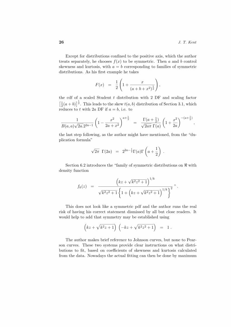
Except for distributions confined to the positive axis, which the authortreats separately, he chooses f(x) to be symmetric. Then a and b controlskewness and kurtosis, with a = b corresponding to families of symmetricdistributions. As his first example he takes

F (x) =12

(1 +

x

(a + b + x2)12

),

the cdf of a scaled Student t distribution with 2 DF and scaling factor[12(a + b)

] 12 . This leads to the skew t(a, b) distribution of Section 3.1, which

reduces to t with 2a DF if a = b, i.e. to

1B(a, a)

√2a.22a−1

(1− x2

2a + x2

)a+ 12

=Γ(a + 1

2)√2aπ Γ(a)

(1 +

x2

2a

)−(a+ 12)

,

the last step following, as the author might have mentioned, from the “du-plication formula”

√2π Γ(2a) = 22a− 1

2 Γ(a)Γ(

a +12

).

Section 6.2 introduces the “family of symmetric distributions on < withdensity function

fk(z) =

(kz +

√k2z2 + 1

)1/k

√k2z2 + 1

{1 +

(kz +

√k2z2 + 1

)1/k}2 ” .

This does not look like a symmetric pdf and the author runs the realrisk of having his correct statement dismissed by all but close readers. Itwould help to add that symmetry may be established using

(kz +

√k2z + 1

) (−kz +

√k2z2 + 1

)= 1 .

The author makes brief reference to Johnson curves, but none to Pear-son curves. These two systems provide clear instructions on what distri-butions to fit, based on coefficients of skewness and kurtosis calculatedfrom the data. Nowadays the actual fitting can then be done by maximum


likelihood methods. In future work the author may want to make somecomparisons and also provide further guidance to the use of his interestingfamilies of distributions.

John T. KentDepartment of Statistics,University of Leeds, U.K.

This paper proposes a new family of distributions motivated by orderstatistics. In addition to the usual location and scale parameters, there aretwo parameters a, b > 0 to model skewness and kurtosis. The methodologyis constructive: given any “base” pdf f(x), symmetric about 0, with range(−∞,∞), and with cdf F (x), new members of the family are given byg(x) ∝ f(x)F a−1(x)[1− F (x)]b−1. Two particular examples for f are usedemphasized in the paper to illustrate this construction: the t distributionwith 2 df (generating the skew t distribution), and the logistic distribution(generating the log F distribution).

These two examples have several additional attractive properties:

1. As noted in the paper, the base pdf satisfies

f(x) = δ{F (x)[1− F (x)]}c, (1)

with c = 1, 3/2 for the logistic and t2 densities, respectively. Theconstant δ can be absorbed in the scale parameter, and hence maybe taken as δ = 1 without any loss of generality. Indeed (1) can bethought of as a differential equation for f , and it can be shown thatthere is a unique solution for each c ≥ 1, with exponential tails forc = 1 and power-law tails for c > 1.

2. The logistic and t2 base measures are normal scale mixtures; that is,each base pdf is a mixture of N(0, σ2) densities, so that f(x) can bewritten in the form

f(x) =∫ ∞

0(2πσ2)−1/2 exp{−x2/(2σ2)}H(dσ2),

for some probability measure H(dσ2) on (0,∞). Further, the mixingdistribution is infinitely divisible (and hence so is the mixture itself)

28 J. T. Kent

in both cases. For more details of these and related properties, seee.g. Barndorff-Nielsen et al. (1982) and Kent (1978). It is not clearto what extent these properties hold for other solutions of (1).

3. The general log F distribution is a normal variance-mean mixture(normal variance mixture if a = b). Also, the symmetric skew t dis-tribution (this is just the usual t distribution with any degrees offreedom) is a normal variance mixture. In both cases the mixingdistribution is infinitely divisible. Here a normal variance-mean mix-ture with real parameter β is a mixture of N(σ2β, σ2) distributions.However, the general skew-t distribution cannot be represented as anormal variance-mean mixture.

Thus, a number of characterization questions and observations arise outof this work.

1. As c varies, to what extent does the base distribution and indeed thewhole order family have the mixing and infinite divisibility propertieslisted above?

2. The use of a suitable mixing distribution in a normal variance-meanmixture is another general recipe for generating wide classes of distri-butions. Barndorff-Nielsen’s generalized hyperbolic distributions (seee.g. Barndorff-Nielsen et al., 1982) are another collection of importantspecial cases in addition to the log F and (symmetric) t-distributions.With modern computers, all these distributions are easy to fit, and adeeper comparision would be welcome.

3. Multivariate skew and long-tailed distributions can also be con-structed using normal variance-mean mixtures. Thus this approachseems to generalize more easily to higher dimensions than does theorder statistics approach.

4. For estimation purposes, the question arises about the uniqueness ofMLEs from these families. Here “MLE” is shorthand for any station-ary point of the likelihood. The (symmetric) tν distribution showsthat the answer can be delicate. Assume the degrees of freedom ν isknown. Then the following results hold (Kent and Tyler, 1991; Kentet al., 1994):


(a) When estimating location only, the MLE is not guaranteed tobe unique.

(b) When estimating location and scale, the MLE will generally beunique if ν ≥ 1. This property fails if ν < 1.

(c) However, if ν is added as a parameter to estimate, it is unclearwhat the uniqueness properties are.

(d) Further, for the skew t distribution, whether or not a and b areassumed known, it is unclear what the uniqueness properties are.

5. Uniqueness properties for some of the other distributions are morestraightforward. The log F and the hyperbolic distributions have logconcave densities. Hence when estimating location and/or scale witha and b held fixed, the MLE will be unique. But again, if a and/or bis to be estimated as well, the uniqueness properties are unclear.

H. N. NagarajaDepartments of Statistics and Internal Medicine

Ohio State University, U.S.A.

Professor Jones introduces here a general family that has interestingdistributional properties and connections as well as potential for excitingstatistical applications. The exposition is thorough and the paper is pre-sented in an informal style by a knowledgeable, well-informed researcher.I enjoyed reading it very much and benefitted tremendously by the insightprovided by Professor Jones and his linking of the numerous results withinthe vast literature on families of distributions. Even the multivariate gen-eralizations are explored; I am waiting to see the forthcoming work, Jonesand Larsen (2004).

As I progressed through the article, two items popped up that I thoughtmight be appropriate for inclusion in this fine contribution to the area ofdistribution theory. They were:

1. Azzalini (1985) skew-normal distribution and its relevance to thisfamily of distributions inspired by the density of order statistics. Re-cently there has been some discussion of nice properties of quadratic

30 J. T. A. S. Ferreira and M. F. J. Steel

forms arising from the multivariate skew-normal distribution of Az-zalini (Genton et al., 2001). It is not clear whether such propertiescould hold for some members of (1) with F = Φ, the standard normalcdf.

2. Application to robustness studies both in terms of skewness and taillength accomplished by an appropriate neighborhood of (1, 1) for the‘shape’ parameter (a, b).

As I reach the last section I discover that both these issues have beenaddressed by Professor Jones in this comprehensive treatment! I only wishhe had more to say on the potential application of this new family in theexamination of robustness of estimators of, say, the location and scale pa-rameters.

I have couple of observations. For an arbitrary F , with either a = 1 orb = 1, from (1.1) we obtain the class of distributions known as “Lehmannalternatives”. So there is one more connection of note. The general familyin (1.1) appears to have a great potential in the power studies of goodness-of-fit tests. When the location and scale parameters are unimportant, thisorder statistic family provides a natural neighborhood for a power study.For example, one can consider such a test for the density f(x) (not neces-sarily symmetric) to be a test of the null hypothesis H0 : a = 1, b = 1, inthe family (1.1) representing the density gF (x; a, b), and explore the powerof the test as a function of (a, b).

Jose T. A. S. Ferreira and Mark F. J. SteelDepartment of Statistics,

University of Warwick, U.K.

We congratulate Professor Chris Jones on a very interesting paper whichprovides an alternative way of generating a large class of distributions.Whereas we are mostly in agreement with the author, we would like tocontribute a few thoughts to the discussion.

The suggested approach provides an elegant interpretation of the classof distributions described through the density function in (1.1) for integerparameters a and b. As the author states, he then extends this by allowingfor any real positive values of a and b. Of course, this extension is no longer


supported by the order statistic interpretation. This suggests that the rela-tion with order statistics is perhaps less fundamental than it appears, eventhough it does help in deriving some of the properties of (1.1). More impor-tantly, the inverse probability integral transform interpretation in Section2.2 is, of course, much more widely applicable, as explored in Ferreira andSteel (2004a), where a very wide class of distributions is proposed.

For brevity, we now focus our comments mostly on the skew t distri-bution, which can accommodate both skewness and fat tails. The authorcorrectly points out that “a and b directly control the relative weights ofthe left- and right-hand tails of the distribution, respectively, so if a 6= b,skewness arises as a ‘secondary’ consequence of having differently weightedtails.” This clearly illustrates the dual roles of a and b. They govern bothtail behaviour and skewness. This raises two related issues. The first is thatof the choice of parametrisation. In this context, the author points out thata reparametrisation proposed by Prentice (1975) seems to improve the be-haviour of the likelihood. An alternative approach would be to restrict theparametrisation of (1.1) to a = γ and b = 1/γ, while perhaps allowing F tobe a distribution with flexible tails. For example, in the particular case ofthe skew t distributions, we could take for F any Student-t distribution, in-dexed by the degrees of freedom ν. Distributions in this class would alwaysbe unimodal, values of γ > 1 generate right skewness, γ < 1 implies leftskewness and the only symmetric member of the class would be the originalStudent-t distribution (i.e. γ = 1). This is illustrated in Figure A, wherewe plot the skewness measure introduced by Arnold and Groeneveld (1995)as a function of γ. The solid line in the figure corresponds to the skew t asin Jones and Faddy (2003) and the dashed line is for the log F distribution.By varying γ, the full range of this skewness measure is covered.

However, even for the alternative class mentioned above the roles of γand ν are not clearly separated, since γ will still influence tail behaviour.In our opinion, this is one (and perhaps the only!) disadvantage of theskew t class, namely that skewness and tail behaviour cannot be modelledindependently. This has potentially quite restrictive consequences. In mod-elling terms, the most important of these is that a skew t distribution cannot simultaneously be very skewed and have heavy tails. As an example,consider the case where the first two moments of GF are required to exist,which is a usual feature to impose in applications. In this case, by the resultin Section 4.5, we need that a, b > 1 and this implies (from the expressionin Jones and Faddy, 2003, Subsection 2.3) that the maximum (minimum)

32 J. T. A. S. Ferreira and M. F. J. Steel

103

10 2

10 1

100

101

102

103

1

0.8

0.6

0.4

0.2

0

0.2

0.4

0.6

0.8

1

γ

Ske

wn

ess

Figure A: Skewness as measured by one minus two times the probability mass left

of the mode as a function of γ (logarithmic scale). Solid line: skew t; dashed line:

log F .

mass assigned to any side of the (unique) mode is approximately 0.78 (0.22).This can clearly be insufficient to accommodate highly skewed data, andthe situation gets even worse if more moments are required to exist. Aspointed out in Ferreira and Steel (2004a) there are a number of alternativeways to model skewness and fat tails where any mass can be assigned to aparticular side of the mode, even after fixing upper bounds on the heavinessof the tails.

Finally, we can provide a few comments on inference with these andsimilar models. We focus particularly on Bayesian inference, since (in acomplementary statement to the author’s) we are not the right people toexplore classical approaches! Ferreira and Steel (2004b) conduct Bayesianinference on regression models using the skew t and a number of otherskewed distributions. They investigate prior elicitation on the basis of priorbeliefs concerning skewness and conduct prior matching for the differentmodels. The parametrisation in terms of a = γ and b = 1/γ is critical in


that skewness is then a monotonic function of γ (as in Figure A) and thisfacilitates prior elicitation considerably. They find that samplers based onMarkov chain Monte Carlo methods can be successfully used for posteriorand predictive inference in these models.

Rejoinder by M. C. Jones

I really am extremely grateful to the discussants of this paper for theirpositive and encouraging remarks and for their insightful comments andquestions. My response will be somewhat uneven as I cherrypick the re-marks to which I think I can usefully respond and do my best to say little ornothing about the others! If, in one or two cases, I appear to ‘pick a fight’,please take my comments in the constructive and, indeed, good-humouredway in which they are intended. I will refer to the individual discussioncontributions by the initial letters of the authors’ surnames thus: Profes-sor Arnold [A], Professor David [D], Mr Ferreira and Professor Steel [FS],Professor Kent [K] and Professor Nagaraja [N].

Starting alphabetically, [A] asks for a “stochastic scenario leading insome way to fractional order statistics” which is partially answered by thereferences given by [D]. The best result yet known is for uniform fractionalorder statistics with n integer, the simplest version of which says that Ua:n ≡(1 − C)Uj:n + CUj+1:n ∼ Beta(a, n + 1 − a) if C ∼ Beta(c, 1 − c), wherea = j + c and j = bac (Papadatos, 1995; Jones, 2002c). There is a link hereto ordinary observed order statistics but it remains unsatisfactory becauseof its ‘externally’ randomised nature (which, I might add, follows a rathermore peculiar distribution than one might have expected).

Both [A] and [N] rightly note that I missed the fact that the specialcases corresponding to a = 1 or b = 1 have been much used in the contextof hypothesis testing under the name “Lehmann alternatives”. Addition ofa reference to Lehmann (1953) is appropriate to make the link for futureScience Citation Index searchers.

A nice point in [D]’s kind remarks is that simple little mathematicaltricks often underlie – and make elegant – certain manipulations, extensionsand properties of distributions. As described in Jones (2001b), it was just

34 M. C. Jones

this kind of thing that started me on the road to the present paper in thefirst place. Having noted that the factorisation 1−x2 = (1+x)(1−x) couldbe construed as leading from symmetric beta distributions to asymmetric(ordinary!) beta distributions (on support [−1, 1]) by allowing differentpowers to be attached to each factor, a similar trick, essentially

11 + x2

= 1− x2

1 + x2=

(1 +

x√1 + x2

) (1− x√

1 + x2

),

led me initially from symmetric Student’s t distributions to the skew tdistributions in this paper.

Comparisons with Pearson and Johnson systems of curves are rightlyasked for by [D]. Here are a few brief remarks pending further investigation.The Pearson system has a direct competitor to the skew t distribution in thePearson Type IV distribution, dismissed by Jones and Faddy (2003, p. 169)as being “more complicated and more difficult to work with”, but probablyworthy of greater respect! The Johnson SU distributions are simpler butdon’t afford the same heavy tails as (skew) t distributions (to such an extentthat all moments exist). Now, both Pearson and Johnson systems alsoinclude distributions on semi-infinite and finite supports. It might be funto try to pad out order statistic distributions similarly in some coherentway. However, I am wary of systems that necessarily match up certaincombinations of skewness and kurtosis with semi-infinite or finite support,regardless of whether these supports are appropriate to the data at hand.Likewise, Johnson SB distributions display bimodality for some skewnessand kurtosis values. Bimodality is the enemy of the distribution theorist!:In my view, bi- and multi-modality should be modelled by mixing unimodaldistributions. In this case, the bimodality problem can be remedied bychanging the basis of Johnson’s distributions from the normal distributionto the logistic (Tadikamalla and Johnson, 1982).

The issue of existence of moments has started to raise its head aboveand in [FS]. I’m afraid I do not view the existence of moments as a partic-ularly important aspect of distribution theory! Obviously, all other thingsbeing equal, existence of moments is nice and helpful, and when they ex-ist they can be informative. But ‘non-existence of moments’ just means‘heavy tails’ in a certain specific sense; this implies the need to use betteralternative measures of location, scale, skewness and/or, in whatever tail-weight/peakedness sense one means it, ‘kurtosis’. Requiring two momentsto exist ([FS]) is, of course, convenient and widespread, for the good reason


that a huge corpus of normal-based theory is then available to assist theanalyst. But if data are better modelled by heavier tails, then shouldn’tthey be modelled by heavier tailed distributions, even if that makes lifetougher?

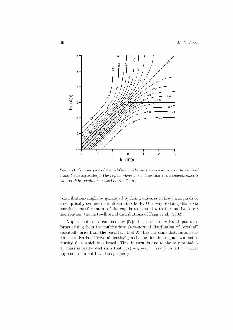
The skewness measure of Arnold and Groeneveld (1995) is just the kindof non-moment-based measure to which I allude above. It is defined for allunimodal distributions and so applies, inter alia, to all skew t distributions,for which it has the explicit formula γM = 1−2I(a+(1/2))/(a+b+1)(a, b). Thisis contour plotted for a wide range of a, b (on log scales) in Figure B.This plot confirms that the skew t distribution can “simultaneously bevery skewed and have heavy tails” (cf. [FS]) provided the very cases thatafford high skewness and heavy tails are not disqualified by requiring twomoments!

I must say that I find [FS]’s alternative skew t family of distributionsintriguing and also highly commend, on a quick first reading, their veryinteresting paper Ferreira and Steel (2004a). I see as complementary twoapproaches to introducing skewness and, if desired, varying kurtosis. Onecategory of methods tries to directly employ a skewness parameter that,in some appropriate sense, is independent of tailweight. This is, perhaps,the most usual approach to skewing symmetric distributions, although as[FS] suggest and Ferreira and Steel (2004a) explore in detail, it is not anentirely trivial trick to pull off. A second category of methods, as here, seesskewness as an implicit consequence of differing left- and right-tailweights.There must be a place in practice for both?

I don’t have a great deal useful to say in response to [K]’s many inter-esting questions and comments. Here are one or two thoughts relating tofamily (1) in his contribution. Kamps (1991) also covers the more generalversion f(x) = F c1(x)(1 − F (x))c2 and I show (Jones, 2002b) that thisdifferential equation is satisfied for all c1, c2 < 0 by what I called the “com-plementary beta distribution” on [0, 1]. This arises from swopping the rolesof the distribution and quantile functions of the beta distribution. Dare Iimagine that, because of the weight of their tails, when c1 = c2 = c ≥ 1, thedistributions are all normal scale mixtures? (But I daren’t offer anythingat all about infinite divisibility!).

[K] and [N] both mention the multivariate case, giving me an excuse toadd to my Section 6.1 that there are also general ways of ‘fixing’ given uni-variate marginals to multivariate ‘bodies’. For example, multivariate skew

36 M. C. Jones

-3 -2 -1 0 1 2 3

log10(a)

-3

-2

-1

0

1

2

3

log

10

(b)

-0.1

-0.1

-0.1

-0.1

-0.2

-0.2

-0.3

-0.3

-0.3

-0.4

-0.4

-0.4

-0.5

-0.5

-0.6

-0.6

-0.7

-0.7

-0.7

-0.8

-0.8

-0.8

-0.9

-0.9

-0.9

0.0

0.0

0.0

0.1

0.1

0.1

0.2

0.2

0.2

0.3

0.3

0.3

0.4

0.4

0.4

0.5

0.5

0.5

0.6

0.6

0.6

0.7

0.7

0.7

0.8

0.8 0.8

0.9

0.9

0.9

Figure B: Contour plot of Arnold-Groeneveld skewness measure as a function of

a and b (on log scales). The region where a, b > 1 so that two moments exist is

the top right quadrant marked on the figure.

t distributions might be generated by fixing univariate skew t marginals toan elliptically symmetric multivariate t body. One way of doing this is viamarginal transformation of the copula associated with the multivariate tdistribution, the meta-elliptical distributions of Fang et al. (2002).

A quick note on a comment by [N]: the “nice properties of quadraticforms arising from the multivariate skew-normal distribution of Azzalini”essentially arise from the basic fact that X2 has the same distribution un-der the univariate ‘Azzalini density’ g as it does for the original symmetricdensity f on which it is based. This, in turn, is due to the way probabil-ity mass is reallocated such that g(x) + g(−x) = 2f(x) for all x. Otherapproaches do not have this property.


I have skipped some very important observations. I applaud [A]’s “in-evitable call ... for more work on problems related to parameter estimation,hypothesis testing and model fitting”, on which [K] makes some interestingobservations and [FS] report some success, at least for their related models.Use of the family in robustness studies and power studies of goodness-of-fittests ([N]) is greatly to be encouraged. Much more in the way of compar-isons between families of distributions ([D], [K]) is also needed. Admittingthat I would join [A]’s “chorus of hisses” but stressing that the remarksthat follow are not for a moment aimed directly at [A] but much morewidely, I would like to add that it is one of the easiest things in the statis-tics research world to come up with more and more mathematical formsfor more and more distributions, many with more and more parameters.The challenge is to select from the panoply of possibilities the most mean-ingful, workable and useful families, keeping the number of parameters toa necessary minimum.

I finish by thanking the Editors very much indeed for their kind invi-tation to prepare this discussion paper and, again, all the discussants fortheir excellent contributions to the discussion.

References

Arnold, B. C., Balakrishnan, N., and Nagaraja, H. N. (1992). AFirst Course in Order Statistics. Wiley, New York.

Arnold, B. C. and Beaver, R. J. (2000). Hidden truncation models.Sankhya, 62:23–35.

Arnold, B. C. and Beaver, R. J. (2002). Skewed multivariate modelsrelated to hidden truncation and/or selective reporting. Test , 11:7–54.

Arnold, B. C. and Groeneveld, R. A. (1995). Measuring skewnesswith respect to the mode. The American Statistician, 49:34–38.

Aroian, L. A. (1941). A study of R. A. Fisher’s z distribution and therelated f distribution. Annals of Mathematical Statistics, 12:429–448.

Azzalini, A. (1985). A class of distributions which includes the normalones. Scandinavian Journal of Statistics, 12:171–178.

38 M. C. Jones

Azzalini, A. and Dalla Valle, A. (1996). The multivariate skew-normaldistribution. Biometrika, 83:715–726.

Balakrishnan, N. (2002). Discussion of “skewed multivariate modelsrelated to hidden truncation and/or selective reporting”. Test , 11:37–39.

Balakrishnan, N. and Akhundov, I. S. (2003). A characterization bylinearity of the regression function based on order statistics. Statisticsand Probability Letters, 63:435–440.

Barlow, R. E. and Proschan, F. (1966). Inequalities for linear combina-tions of order statistics from restricted families. Annals of MathematicalStatistics, 37:1574–1592.

Barlow, R. E. and Proschan, F. (1975). Statistical Theory of Reliabilityand Life Testing; Probability Models. Holt, Rhinehart and Winston, NewYork.

Barndorff-Nielsen, O., Kent, J., and Sørensen, M. (1982). Normalvariance-mean mixtures and z distributions. International Statistical Re-view , 50:145–159.

Birnbaum, A. and Dudman, J. (1963). Logistic order statistics. Annalsof Mathematical Statistics, 34:658–663.

Box, G. E. P. and Tiao, G. C. (1973). Bayesian Inference in StatisticalAnalysis. Addison-Wesley, Reading, MA.

Brown, B. W., Spears, F. M., and Levy, L. B. (2002). The log F : adistribution for all seasons. Computational Statistics, 17:47–58.

David, H. A. and Nagaraja, H. N. (2003). Order Statistics. Wiley,Hoboken, NJ, 3rd ed.

Devroye, L. (1986). Non-Uniform Random Variate Generation. Springer,New York.

Duncan, A. J. (1986). Quality Control and Industrial Statistics. Irwin,Homewood, Illinois, 5th ed.

Durrans, S. R. (1992). Distributions of fractional order statistics inhydrology. Water Resources Research, 28:1649–1655.


Eugene, N. (2001). A generalized normal distribution: properties, estima-tion and applications. Ph.D. thesis, Central Michigan University.

Eugene, N., Lee, C., and Famoye, F. (2002). Beta-normal distribu-tion and its applications. Communications in Statistics – Theory andMethods, 31:497–512.

Fang, H. B., Fang, K. T., and Kotz, S. (2002). The meta-ellipticaldistributions with given marginals. Journal of Multivariate Analysis,82:1–16.

Ferreira, J. T. and Steel, M. F. J. (2003). Bayesian multivariateregression analysis with a new class of skewed distributions. TechnicalReport UKC/IMS/03/28, University of Kent.

Ferreira, J. T. A. S. and Steel, M. F. J. (2004a). A constructiverepresentation of univariate skewed distributions. Statistics ResearchReport 422, University of Warwick.

Ferreira, J. T. A. S. and Steel, M. F. J. (2004b). Model comparisonof coordinate-free multivariate skewed distributions with an applicationto stochastic frontiers. Statistics Research Report 423, University ofWarwick.

Fisher, R. A. (1924). On a distribution yielding the error functions ofseveral well known statistics. In Proceedings of the International Mathe-matical Congress, vol. 2, pp. 805–813. Toronto.

Genton, M. G., He, L., and Liu, X. (2001). Moments of skew-normalrandom vectors and their quadratic forms. Statistics and ProbabilityLetters, 51:319–325.

Greenland, S. (2001). Putting background information about relativerisks into conjugate prior distributions. Biometrics, 57:663–670.

Greenwood, J. A., Landwehr, J. M., Matalas, N. C., and Wallis,J. R. (1979). Probability weighted moments: Definition and relation toparameters of several distributions expressible in inverse form. WaterResources Research, 15:1049–1054.

Gupta, R. D. and Kundu, D. (1999). Generalized exponential distribu-tions. Australian and New Zealand Journal of Statistics, 41:173–188.

40 M. C. Jones

Gupta, R. D. and Kundu, D. (2001a). Exponentiated exponential family:An alternative to gamma and Weibull distributions. Biometrical Journal ,43:117–130.

Gupta, R. D. and Kundu, D. (2001b). Generalized exponential distribu-tion: Different method of estimations. Journal of Statistical Computationand Simulation, 69:315–337.

Gupta, R. D. and Kundu, D. (2003a). Closeness of gamma and gener-alized exponential distribution. Communications in Statistics – Theoryand Methods, 32:705–721.

Gupta, R. D. and Kundu, D. (2003b). Discriminating between Weibulland generalized exponential distributions. Computational Statistics andData Analysis, 43:179–196.

Gupta, R. D. and Shah, B. K. (1965). Exact moments and percentagepoints of the order statistics and the distribution of the range from thelogistic distribution. Annals of Mathematical Statistics, 36:907–920.

Huillard d’Aignaux, J. N., Cousens, S. N., and Smith, P. G. (2003).The predictability of the epidemic of variant Creutzfeldt-Jacob diseaseby back-calculation methods. Statistical Methods in Medical Research,12:203–220.

Johnson, N. L. and Kotz, S. (1972). Distributions in Statistics: Con-tinuous Multivariate Distributions. Wiley, New York.

Johnson, N. L. and Kotz, S. (1973). Extended and multivariate Tukeylambda distributions. Biometrika, 60:655–661.

Johnson, N. L., Kotz, S., and Balakrishnan, N. (1995). ContinuousUnivariate Distributions, vol. 2. Wiley, New York, 2nd ed.

Jones, M. C. (2001a). Multivariate t and beta distributions associatedwith the multivariate F distribution. Metrika, 54:215–231.

Jones, M. C. (2001b). A skew t distribution. In C. A. Charalambides,M. V. Koutras, and N. Balakrishnan, eds., Probability and StatisticalModels with Applications, pp. 269–278. Chapman and Hall/CRC, Lon-don.


Jones, M. C. (2002a). Changing marginals of multivariate densities bymultiplication, with application to skewing spherically symmetric distri-butions. Journal of Multivariate Analysis, 81:85–99.

Jones, M. C. (2002b). The complementary beta distribution. Journal ofStatistical Planning and Inference, 104:329–337.

Jones, M. C. (2002c). On fractional uniform order statistics. Statisticsand Probability Letters, 58:93–96.

Jones, M. C. (2002d). Student’s simplest distribution. Journal of theRoyal Statistical Society, Series D , 51:41–49.

Jones, M. C. and Faddy, M. J. (2003). A skew extension of the tdistribution, with applications. Journal of the Royal Statistical Society,Series B , 65:159–174.

Jones, M. C. and Larsen, P. V. (2004). Multivariate distributions withsupport above the diagonal. Biometrika. To appear.

Kamps, U. (1991). A general recurrence relation for moments of orderstatistics in a class of probability distributions and characterizations.Metrika, 38:215–225.

Kent, J. T. (1978). Some probabilistic properties of Bessel functions.Annals of Probability , 6:760–770.

Kent, J. T. and Tyler, D. E. (1991). Redescending m-estimates ofmultivariate location and scatter. Annals of Statistics, 19:2102–2119.

Kent, J. T., Tyler, D. E., and Vardi, Y. (1994). A curious likelihoodidentity for the multivariate t distribution. Communications in Statistics:Simulation and Computation, 23:441–453.

Lange, K. L., Little, R. J. A., and Taylor, J. M. G. (1989). Robuststatistical modelling using the t distribution. Journal of the AmericanStatistical Association, 84:881–896.

Lehmann, E. L. (1953). The power of rank tests. Annals of MathematicalStatistics, 24:23–43.

Numerical Algorithms Group (2003). NAG FORTRAN libraries.

42 M. C. Jones

Olkin, I. and Liu, R. (2003). A bivariate beta distribution. Statistics andProbability Letters, 62:407–412.

Papadatos, N. (1995). Intermediate order statistics with applications tononparametric estimation. Statistics and Probability Letters, 22:231–238.

Patel, J. K. and Read, C. B. (1982). Handbook of the Normal Distribu-tion. Dekker, New York.

Peng, Y., Dear, K. B. G., and Denham, J. W. (1998). A generalized Fmixture model for cure rate estimation. Statistics in Medicine, 17:813–830.

Prentice, R. L. (1975). Discrimination among some parametric models.Biometrika, 62:607–614.

Ratnaparkhi, M. V. and Mosimann, J. E. (1990). On the normality oftransformed beta and unit-gamma random-variables. Communicationsin Statistics – Theory and Methods, 19:3833–3854.

Reiss, R. D. (1989). Approximate Distributions of Order Statistics; withApplications to Nonparametric Statistics. Springer, New York.

Rohatgi, V. K. and Saleh, A. K. M. E. (1988). A class of distributionsconnected to order statistics with nonintegral sample size. Communica-tions in Statistics – Theory and Methods, 17:2005–2012.

Rydberg, T. H. (2000). Realistic statistical modelling of financial data.International Statistical Review , 68:233–258.

Samorodnitsky, G. and Taqqu, M. S. (1994). Stable Non-GaussianRandom Processes; Stochastic Models with Infinite Variance. Chapmanand Hall/CRC, Boca Raton.

Smyth, G. K. (1994). A note on modelling cross-correlations: Hyperbolicsecant regression. Biometrika, 81:396–402.

Stigler, S. M. (1977). Fractional order statistics, with applications. Jour-nal of the American Statistical Association, 72:544–550.

Tadikamalla, P. K. (1980). Random sampling from the exponentialpower distribution. Journal of the American Statistical Association,75:683–686.


Tadikamalla, P. K. and Johnson, N. L. (1982). Systems of frequencycurves generated by transformations of logistic variables. Biometrika,69:461–465.

Vaughan, D. C. (1992). Expected values, variances and covariances oforder statistics for Student’s t–distribution with two degrees of freedom.Communications in Statistics – Simulation and Computation, 21:391–404.

Wand, M. P. and Jones, M. C. (1995). Kernel Smoothing . Chapmanand Hall, London.

Sociedad Española de Estadística e Investigación Operativa ... · e Investigación Operativa...

Documents

Transcript of Sociedad Española de Estadística e Investigación Operativa ... · e Investigación Operativa...