Trabajo Fin de Grado Ingeniería Aeroespacial Análisis ...

Trabajo Fin de Grado

Ingeniería Aeroespacial

Numerical Analysis on DEFORM-3D of limit strains

in Single Point Incremental Forming for AISI304-

H111 sheets

Autor: Álvaro Fernández Díaz

Tutor: Gabriel Centeno Báez

Departamento de Ingeniería Mecánica y

Fabricación

Escuela Técnica Superior de Ingeniería

Universidad de Sevilla


Sevilla, 2016

Análisis numérico en DEFORM-3D de deformaciones

límite en conformado incremental mono-punto de

chapas de acero AISI304-H111

iii

Trabajo Fin de Grado


Numerical Analysis on DEFORM-3D of limit strains in

Single Point Incremental Forming for AISI304-H111

sheets

Autor:

Álvaro Fernández Díaz

Tutor:

Gabriel Centeno Báez

Profesor Contratado Doctor

Departamento de Ingeniería Mecánica y Fabricación



Sevilla, 2016

iv

Proyecto Fin de Grado: Numerical Analysis on DEFORM-3D of limit strains in Single Point Incremental

Forming for AISI304-H111 sheets



El tribunal nombrado para juzgar el Proyecto arriba indicado, compuesto por los siguientes miembros:

Presidente:

Vocales:

Secretario:

Acuerdan otorgarle la calificación de:

Sevilla, 2016

El Secretario del Tribunal

v

A mis abuelos

vii

Agradecimientos

A mis padres, porque sin su apoyo no habría podido llegar a estudiar esta carrera.

A mis amigos, por aguantarme y apoyarme en cada paso del camino.

A mi tutor Gabriel Centeno Báez, por haberme permitido realizar este proyecto con él, a pesar haber estado

fuera, y de lo apretado de su agenda, y por su disposición a sacar un rato para ayudarme y resolverme las

dudas siempre que le era posible.

A los miembros del departamento de Ingeniería Mecánica y Fabricación, especialmente a Marcos Borrego

Puche, fundamental apoyo en mis primeros pasos con DEFORM™-3D, y a Andrés Jesús Martínez Donaire,

por estar siempre dispuesto a ayudarme con cualquier duda que me surgiese.

A mi profesor del Bachillerato Internacional Jesús Moreno, por mostrarme el maravilloso mundo de la física y

la ingeniería.

Y finalmente, a mi compañero y amigo Pedro Grau Morgado, por su apoyo y camaradería estos años, y por

demostrarme que con empeño y dedicación, todo es posible.

Álvaro Fernández Díaz

Sevilla, 2016

ix

Resumen

El principal objetivo de este proyecto es crear un modelo numérico para placas de acero AISI304-H111

conformadas mediante procesos de conformado incremental mono-punto (SPIF), y validarlo en términos de

deformaciones con los resultados experimentales obtenidos previamente por el grupo de investigación del

Área de Ingeniería de los Procesos de Fabricación del Departamento de Ingeniería Mecánica y Fabricación de

la Universidad de Sevilla. El modelo se realizará en DEFORM™-3D, conocido por ser un software robusto

basado en la mecánica de los elementos finitos (FEM), que usa cálculo implícito y tiene una gran aplicación

industrial.

El documento está estructurado en tres secciones principales. Comienza comentando los distintos métodos de

conformado incremental de chapas (ISF), describiendo con más detalle las características y aplicaciones del

SPIF, para acabar estableciendo los principales objetivos del proyecto y revisando los antecedentes

experimentales.

La segunda sección es un conciso manual paso a paso que enseña cómo usar DEFORM™-3D, concretamente

cómo crear el modelo numérico para los procesos de conformado incremental llevados a cabo en este

proyecto.

Finalmente, en la tercera sección, se exponen los resultados y se analizan en términos de deformaciones, para

compararlos con los resultados experimentales previamente mencionados, validando así el modelo.

xi

Abstract

The main objective in this project is to create a Single Point Incremental Forming (SPIF) process numerical

model for AISI304-H111 sheets, and validate it in strain terms with experimental data previously obtained by

the group of Manufacturing at the Department of Mechanical Engineering and Manufacturing at the

University of Seville. The model will be carried out on DEFORM™-3D, which is known for being a robust

FEM-based software, having a great industrial application and using implicit computation.

The document is structured in three main sections. It starts by commenting different ISF methods, describing

in more detail the characteristics and applications on the SPIF, to finish by establishing the main objectives of

the project, and reviewing the backgrounds.

The second section is a concise step by step manual guide to show how to use DEFORM™-3D, specifically

how to create a numerical model for the incremental forming processes carried out in this project.

Finally, in the third section, the results were exposed and analysed in strain terms, in order to compare them

with the previously commented experimental results, validating the model.

xiii

Index

Agradecimientos .......................................................................................................................................... vii

Resumen ....................................................................................................................................................... ix

Abstract ........................................................................................................................................................ xi

Index ........................................................................................................................................................... xiii

1 Tables Index .......................................................................................................................................... xv

2 Figures Index ....................................................................................................................................... xvii

1 INTRODUCTION ................................................................................................................................... 21 1.1 Forming Limit Diagram ............................................................................................................................. 21

1.1.1 The Nakazima stretching test ........................................................................................................... 24 1.2 Incremental sheet forming processes ...................................................................................................... 25

1.2.1 Spinning .............................................................................................................................................. 25 1.2.2 Single Point Incremental Forming (SPIF) .......................................................................................... 26 1.2.3 Incremental Forming With Counter Tool (IFWCT) .......................................................................... 27 1.2.4 Two Point Incremental Forming (TPIF) ............................................................................................ 27 1.2.5 Multistage Forming ........................................................................................................................... 28

1.3 Single Point Incremental Forming characteristics ................................................................................... 29 1.3.1 The forming tool ................................................................................................................................ 29 1.3.2 The blank holder ................................................................................................................................ 30 1.3.3 Incremental Forming machinery ...................................................................................................... 31 1.3.4 SPIF’s advantages and disadvantages .............................................................................................. 32

1.4 Background ................................................................................................................................................ 33 1.5 Project’s objectives .................................................................................................................................... 35

2 DEFORM™-3D ...................................................................................................................................... 37 2.1 DEFORM™-3D as a numeric tool. ............................................................................................................. 38

3 RESULTS ............................................................................................................................................... 53 3.1 20 mm diameter tool ................................................................................................................................. 53 3.2 10 mm diameter tool ................................................................................................................................. 58 3.3 Accumulated damage ............................................................................................................................... 62

3.3.1 20 mm diameter tool ........................................................................................................................ 64 3.3.2 10 mm diameter tool ........................................................................................................................ 65

4 CONCLUSIONS AND FUTURE DEVELOPMENTS..................................................................................... 67 4.1 Conclusions ................................................................................................................................................. 67 4.2 Future developments ................................................................................................................................. 68

REFERENCES ................................................................................................................................................ 69

xv

1 Tables Index

Table 2-1 Mechanical properties of the AISI 304 metal sheets 39

Table 3-1 Parameters of interest during different remeshings 57

Table 3-2 Strain fracture and experimental critical damage values 64

xvii

2 Figures Index

Figure 1.1 Different states of the principal strains 22

Figure 1.2 Different states of the principal strains 22

Figure 1.3 FLC curves for high ductility (a) and low ductility (b) materials 23

Figure 1.4 Forming limit diagram (FLD) based on conventional Nakazima tests containing the

forming limit curve (FLC) and the fracture forming line (FFL) for 0.8 mm thickness AISI 304 metal

sheets 24

Figure 1.5 (a) Erichsen universal sheet metal testing machine, (b) scheme of the experimental setup

and (c) specimen geometries before and after testing 25

Figure 1.6 Spinning schematics 26

Figure 1.7 Structural differences between conventional and shear spinning 26

Figure 1.8 Schematic representation of a SPIF process 27

Figure 1.9 Schematic representation of an IFWCT process 27

Figure 1.10 TPIF schematics with (a) partial die and (b) total die 28

Figure 1.11 Multistage forming example 28

Figure 1.12 Multistage strategy formulated by Skjoedt et al. (2008) 29

Figure 1.13 Geometry without revolution axis achieved with multistage forming. 29

Figure 1.14 SPIF forming tool 30

Figure 1.15 Blank holder and backing plate used in a SPIF process 30

Figure 1.16 3-axial CNC machine 31

Figure 1.17 SPIF dedicated machine 31

Figure 1.18 Robotic Incremental Sheet Metal Forming 32

Figure 1.19 Stewart Platform 32

Figure 1.20 Spifability of the AISI 304 metal sheets using tool diameters of 10 and 20 mm for step

downs of 0.2 and 0.5 mm per pass. 33

Figure 1.21 Fractography of the failure zone in stretch-bending using a cylindrical punch of 20 mm

(left) and 10 mm (right) diameter, respectively. 34

Figure 1.22 (a) Testing geometry used in SPIF, (b) point pattern on the final part and (c) contour of

major principal strain obtained from ARGUS® and (d) cut final part ready for measuring thickness

along the crack. 34

Figure 2.1 Pre-processor 38

Figure 2.2 Simulation Controls (SI units) 38

Figure 2.3 Main toolbar on the pre-processor 39

Figure 2.4 Material window 39

Figure 2.5 Behaviour law generator 40

Figure 2.6 Fracture method 40

Figure 2.7 Object type and material choosing 41

xviii

Figure 2.8 Geometry selection 41

Figure 2.9 Sheet geometry data 42

Figure 2.10 Tool geometry data 42


Figure 2.12 Pre-processor drag control 43

Figure 2.13 Pre-processor interference control 43

Figure 2.14 Simulation geometry correctly positioned 44

Figure 2.15 Sheet meshing 44

Figure 2.16 Detailed meshing settings 45

Figure 2.17 Different meshing windows 45

Figure 2.18 Problem with the meshing 46

Figure 2.19 Final meshing for the 20mm tool 46

Figure 2.20 Simulation failure with the blank holder 47

Figure 2.21 Boundary conditions in x and y directions (a) and in z direction (b) 48

Figure 2.22 Tool trajectory with the step down 48

Figure 2.23 Movement window in the pre-processor 49

Figure 2.24 Point cloud of the trajectory 49


Figure 2.26 Inter object and friction window 50

Figure 2.27 Step number selection 51

Figure 2.28 Step increment control number selection 51


Figure 2.30 Database checking and generation 52

Figure 3.1 Mayor strain distribution in the outer surface of a SPIF formed AISI304 sheet with a 20

mm diameter tool 53

Figure 3.2 Mayor strain distribution along a dot line in the outer surface of a SPIF formed AISI304

sheet with a 20 mm diameter tool 54

Figure 3.3 Minor strain distribution in the outer surface of a SPIF formed AISI304 sheet with a 20 mm

diameter tool 55

Figure 3.4 Minor strain distribution along a dot line in the outer surface of a SPIF formed AISI304


Figure 3.5 Experimental and numeric results of the formability until fracture of a SPIF formed

AISI304 sheet with a 20 mm diameter tool 56

Figure 3.6 Final geometry of a SPIF formed AISI304 sheet with a 20 mm diameter tool 58

Figure 3.7 Final geometry of a SPIF formed AISI304 sheet with a 10 mm diameter tool 58

Figure 3.8 Mayor strain distribution in the outer surface of a SPIF formed AISI304 sheet with a 10

mm diameter tool 59

Figure 3.9 Mayor strain distribution along a dot line in the outer surface of a SPIF formed AISI304


Figure 3.10 Minor strain distribution in the outer surface of a SPIF formed AISI304 sheet with a 10

mm diameter tool 60

Figure 3.11 Minor strain distribution along a dot line in the outer surface of a SPIF formed AISI304

xix


Figure 3.12 Experimental and numeric results of the formability until fracture of a SPIF formed


Figure 3.13 Fracture modes; respectively, Mode I, Mode II, and Mode III 62

Figure 3.14 Crack propagation in fracture Mode I 63

Figure 3.15 Distribution of the accumulated damage according the Ayada criterion on a SPIF formed


Figure 3.16 Distribution of the accumulated damage according the Ayada criterion on a SPIF formed


21

1 INTRODUCTION

Sheet forming in current industry is a high used process among a large group of production sectors, so that it’s

in continuous progress and revision.

For example, in the aeronautical sector, sheet stretching is used to form the body of the aeroplanes, needing

high specialized equipment and tools. That’s why this technology is only profitable with a large scale of

production.

Incremental sheet forming is an innovative process that fulfils the current requirements for flexible, sustainable

and economic manufacturing technologies viable for small and medium-sized batches, not being necessary the

use of expensive dedicated machines or equipment.

Single-Point Incremental Forming (SPIF) is the simplest manufacturing process among those based on

incremental forming of a metal sheet. It consists on a hemispherical end forming tool driven by a Computer

Numerical Control (CNC) machine that follows progressively a pre-established trajectory, deforming

plastically a peripherally clamped sheet blank into a final component, without the use of a forming die during

the process. That allows a better formability, plus the other advantages formerly mentioned.

This Project will calculate numerically with a Finite Element Method (FEM) program, DEFORM™-3D, the

strain evolution on an AISI304 sheet, with 10mm and 20mm tools. That, under some hypothesis, will allow to

have a model to compare with experimental results obtained by Centeno et al (2014), and also provide the

stress distribution on the sheet.

1.1 Forming Limit Diagram

The main used tool to measure the formability of a metal sheet is the Forming Limit Diagram, proposed by

Keeler and Backhofen (1963), and Goodwin (1968). This diagram depicts the Forming Limit Curve, which

shows mayor and minor principal strains limit values in the sheet plane, needed to create the failure under

different strain relations.

Marciniak (2002) established that the formability is related with the strain state. If it’s assumed that the total

sum of the three mayor strains, 𝜀1, 𝜀2, 𝜀3 equals zero, because of volume constancy, plus it’s only needed to

know two of them, related by the following expression:

𝜀2 = 𝛽𝜀1

22

There are several strain cases of interest, distinguished by the value of β, as explained:

- 𝛽 = 1, in this case, 𝜀1 = 𝜀2, with constant strain in every direction in an equi-biaxial state.

- 𝛽 = 0, there is no minor strain, 𝜀2 = 0, being known as plane-strain.

- 𝛽 = −0.5, this is the state present in tensile tests of isotropic materials, known as uniaxial.

- 𝛽 = −1, here 𝜀1 + 𝜀2 = 0, and consequently, 𝜀1 = 0, there is no variation in the thickness. This state

is known as deep drawing.

These states are represented in the following figure:

Figure 1.1 Different states of the principal strains

The FLC usually shows a necking failure curve, generally in ductile materials. In Figure 1.2 can be seen the

evolution of that curve for different materials. It’s worth to mention that the lowest value of the curve, known

as FLC(0), is a characteristic data of the material, which occurs under plane strain conditions.

Figure 1.2 Different states of the principal strains

23

Plus it’s usually added a ductile fracture curve above the necking curve. As it depends on the ductility of the

material, on very ductile materials it will be a decreasing straight line, while in low ductility materials will be

similar to the necking failure curve, approaching to equi-biaxials strain conditions, and therefore showing that

the material will reach fracture with almost no necking.

(a) (b)

Figure 1.3 FLC curves for high ductility (a) and low ductility (b) materials

Nowadays, the numeric computer calculation for both the numeric evaluation of the sheet forming process and

the numeric estimation of the FLD, allowing then to compare it with the experimental curves. For good results

on the forming diagrams, several experimental tests, and simulations to contrast results. These tasks are

necessary to create a failure criterion of the material that allows forming in a safe strain range. That’s why this

project will simulate something already analysed experimentally.

There is a wide variety of ductile fracture criteria on scientific literature. Some studies proved that continuous

fracture criteria (integral criteria) predict correctly the lineal FFL. However, those criteria are not capable of

reproduce the seen FFL for low ductility metal sheets, with either a V-shaped curve or a complex form in the

necking area. In those cases, it has been proved that failure criteria based on tangential stresses, such as Tresca

or Bressan approximates well the experimental FFL in a wide range of strain relations. Those diagrams will be

obtained performing several tests, such a stress tests, stretching tests and stretch-bending tests. One example of

an experimental Forming Limit Diagram is the one obtained by the previously mentioned paper (on which this

project is based), Centeno et al. (2014):

24

Figure 1.4 Forming limit diagram (FLD) based on conventional Nakazima tests containing the forming limit

curve (FLC) and the fracture forming line (FFL) for 0.8 mm thickness AISI 304 metal sheets

1.1.1 The Nakazima stretching test

This test consists on taking a previously prepared sample and setting it in the blank holder. Then, the top die is

placed on the sheet sample and secured to hold the system. Then a previously lubricated hemispherical punch

of 100 mm of diameter rises at constant speed to form the sample until failure occurs.

This is the most used stretching test, being used as a reference on the ISO12004-2, which standardizes the

construction of forming limit curves (FLC) on laboratories, both on the testing parameters and the

methodology to detect the onset of localised necking. This part of the ISO12004 specifies the testing

conditions to be used when constructing a forming limit curve (FLC) at ambient temperature and using linear

strain paths.

The considered material is flat, metallic and of thickness between 0.3 mm and 4 mm, being the recommended

thickness for steel of 2.5 mm. It also standardizes the rest of the test conditions, such as lubrication, punch

velocity or specimen geometries. Regarding the geometry, it’s recommended to use notched specimens with a

calibrated central part, with a 25% bigger length than the punch diameter.

25

Figure 1.5 (a) Erichsen universal sheet metal testing machine, (b) scheme of the experimental setup and (c)

specimen geometries before and after testing

1.2 Incremental sheet forming processes

Just as Schmoeckel (1992) predicted, automatization has made forming processes more flexible.

The ISF deforms gradually a metal sheet with one only tool, guided by a Computer Numeric Control machine,

allowing to obtain many different geometries. It allows fast prototyping, needing short times on design and

manufacturing. That makes those processes very profitable for the production of small batches of pieces.

Nowadays there are plenty of different metal forming processes that use an incremental approach. As said

before, in those processes the material forming is produced incrementally, and only in a small area of the sheet,

therefore needing smaller forces compared to traditional processes. Now some of them will be commented.

1.2.1 Spinning

In the spinning, the metal sheet is embedded on a spinning mandrel. While the sheet is rotating, the tool

approaches progressively forming it to the desired geometry. The tool has a roller geometry, and can be

actuated either manually or mechanically (a lathe is needed for that). This is one of the oldest processes, being

created in the Middle Age.

26

Figure 1.6 Spinning schematics

There is a variant, known as shear spinning, where the sheet isn’t bent, but stretched, reducing its thickness,

fulfilling the Sine Law:

𝑡𝑓 = 𝑡0 ∗ 𝑠𝑒𝑛 (𝜋

2− 𝛼)

Figure 1.7 Structural differences between conventional and shear spinning

1.2.2 Single Point Incremental Forming (SPIF)

The idea of gradually forming with only one point tool was already patented by Leszak (1967), which was a

visionary, since in that time it wasn’t possible to do it. Single Point Incremental Forming process is a great

progress compared to spinning, because it allows to create not axisymmetric geometries. In this process, the

metal sheet is held between a blank holder and a backing plate. The tool will be controlled by a CNC machine,

and it moves along the designed trajectory to describe the final geometry of the desired piece. In this process,

27

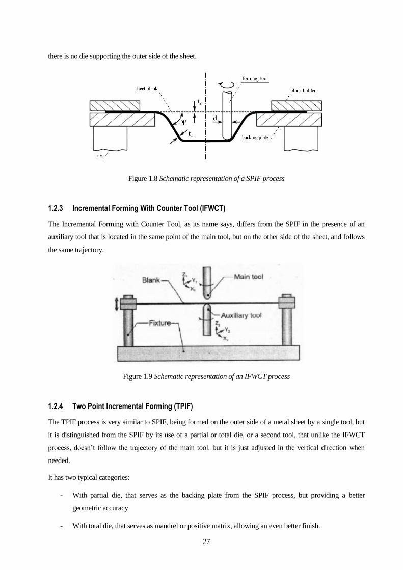
there is no die supporting the outer side of the sheet.

Figure 1.8 Schematic representation of a SPIF process

1.2.3 Incremental Forming With Counter Tool (IFWCT)

The Incremental Forming with Counter Tool, as its name says, differs from the SPIF in the presence of an

auxiliary tool that is located in the same point of the main tool, but on the other side of the sheet, and follows

the same trajectory.

Figure 1.9 Schematic representation of an IFWCT process

1.2.4 Two Point Incremental Forming (TPIF)

The TPIF process is very similar to SPIF, being formed on the outer side of a metal sheet by a single tool, but

it is distinguished from the SPIF by its use of a partial or total die, or a second tool, that unlike the IFWCT

process, doesn’t follow the trajectory of the main tool, but it is just adjusted in the vertical direction when

needed.

It has two typical categories:

- With partial die, that serves as the backing plate from the SPIF process, but providing a better

geometric accuracy

- With total die, that serves as mandrel or positive matrix, allowing an even better finish.

28

(a) (b)

Figure 1.10 TPIF schematics with (a) partial die and (b) total die

1.2.5 Multistage Forming

For each specific material and thickness sheet, the maximum forming angle can be easily obtained in a test

where the final geometry is a cone with variable generatix angle, keeping constant the rest of the variables. It’s

easy to check that it’s impossible to produce pieces with right angles, because according to the Sine Law, its

final thickness would be zero.

One way to enhance this angle is to increase the initial thickness of the sheet, but it would create problems, in

the formability and in the necessary loading capacity of machines and tools. The step down and the tool

diameter also affects, but the mainly final solution was to generate trajectories with several stages in which the

forming angle is being increased.

Figure 1.11 Multistage forming example

29

Recently, Skjoedt et al. (2008) proposed a solution to obtain vertical walls cones based on this process,

realized with 5 stages:

Figure 1.12 Multistage strategy formulated by Skjoedt et al. (2008)

Also, Duflou et al.(2005) used multistage forming strategies in order to create geometries without revolution

axis.

Figure 1.13 Geometry without revolution axis achieved with multistage forming.

1.3 Single Point Incremental Forming characteristics

1.3.1 The forming tool

The main element in this process is the solid tool with a semi spherical tip, which assures a continuous contact

in the sheet point where it’s plastically formed. In some cases, with sharp wall angles, might be needed a

smaller stem than the tool diameter of the spherical tip, avoiding that way the contact between the stem and the

sheet.

In most cases, these tools are made of steel. Since the biggest heat source is friction, to reduce it, and therefore

increase its useful life, it’s usually lubricated. It can be covered or even totally made by some material with

greater hardness, such as cemented carbide, reducing the tool weathering.

A wide range of tool diameters is used, going from small diameters of 6 mm to 100 mm of diameter, used this

last one to manufacture larger pieces. Naturally, they need much more power due to the much bigger contact

angle. It affects the final surface finish and the manufacturing time, being the tool diameter determined by the

smallest concave radius required in the geometry.

30

Figure 1.14 SPIF forming tool

1.3.2 The blank holder

The blank holder is used to firmly hold the sheet during the forming, restricting the displacement. It also has a

backing plate, which guides the sheet material in the correct direction in the process. As mentioned before, in

the TPIF case, the die (that works as backing plate), can move along the vertical direction.

Figure 1.15 Blank holder and backing plate used in a SPIF process

31

1.3.3 Incremental Forming machinery

In SPIF processes, the main force applied is the axial one, needing a previous estimation to ensure the correct

behaviour of the machine. Usually, any 3-axial CNC machine is suitable to form in SPIF.

Figure 1.16 3-axial CNC machine

Their high velocities, allowing large workloads and stiffness make them ideal for SPIF. There are different

designs, differing on their workload, maximum velocity, maximum load, stiffness and cost, allowing to choose

the necessary one according to the necessities.

Nowadays, there is only one company that has created a specifically designed SPIF machine (Hirt, 2004). It

has a high feed rate and allows medium sized workloads. It’s based on the technology developed by Amino et

al. (2002) including an Aoyama et al. (2000) patent:

Figure 1.17 SPIF dedicated machine

There are plenty other machines potentially suitable. Industrial robots are being tested (Figure 1.18) that admit

huge workloads, low stiffness and acceptable maximum loads. Several institutes are trying to apply industrial

robots to incremental forming such as Schafer et al. (2004) and Meier et al. (2005). This forming method is yet

in its primary phase. One special setup in robot forming is to use incremental hammer fisting instead of a

continuously moving rigid tool. In this case, the forming tool describes a fast oscillating movement, which

gives the desired geometry to the sheet.

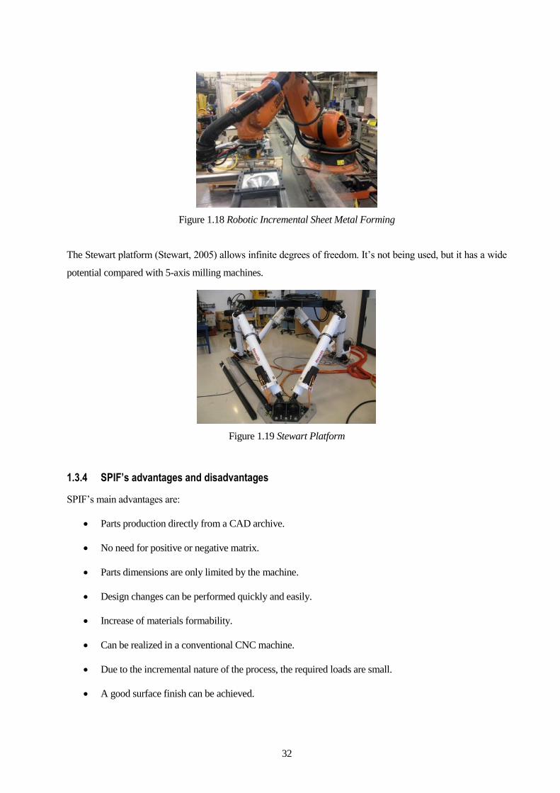
32

Figure 1.18 Robotic Incremental Sheet Metal Forming

The Stewart platform (Stewart, 2005) allows infinite degrees of freedom. It’s not being used, but it has a wide

potential compared with 5-axis milling machines.

Figure 1.19 Stewart Platform

1.3.4 SPIF’s advantages and disadvantages

SPIF’s main advantages are:

Parts production directly from a CAD archive.

No need for positive or negative matrix.

Parts dimensions are only limited by the machine.

Design changes can be performed quickly and easily.

Increase of materials formability.

Can be realized in a conventional CNC machine.

Due to the incremental nature of the process, the required loads are small.

A good surface finish can be achieved.

33

Regarding its disadvantages, the following can be mentioned:

Longer processing time compared with conventional deep drawing.

Limited to small production batches.

The creation of right angles must be achieved by several stages.

Worse geometric accuracy, especially in edges and convex bending radius.

There is elastic recuperation, although it can be minimized using some specific correction

algorithms.

1.4 Background

The increase of the formability of metal sheets with ISF processes, specifically Single Point Incremental

Processes, has been experimentally studied by several authors, such as Emmens et al. (2009), Jeswiet et al.

(2010) or Silva et al (2011) among others.

The Fabrication Engineering Process investigation group from the Seville’s University Mechanic Engineering

Department has been researching and performing numerous tests and numeric simulations about metallic sheet

forming, specifically the influence of the flexion in forming processes, evaluating failure mechanisms and

researching what parameters affect them, as in Centeno et al. (2012).

Under that line of research, a methodology has been developed to obtain limit forming diagrams, for both

stretching, and stretching with flexion situations. That methodology has been tested for several materials, such

as AA7075-O, AA2024-T3, or AISI304-H111 among others.

Specifically, that last material will be analysed in this project. In Centeno et al (2014), there was obtained the

following strain evolution on SPIF on the outer surface of the AISI304 sheet, once the failure took place.

Figure 1.20 Spifability of the AISI 304 metal sheets using tool diameters of 10 and 20 mm for step downs of 0.2

and 0.5 mm per pass.

34

Several different tests were carried out, with tools of 6mm, 10 mm and 20 mm diameter. For each tool

diameter, the step down was alternatively set to 0.2 mm and 0.5 mm per pass. Three replicates of each SPIF

test were carried out, that gave almost the same results.

The final strain state was measured with ARGUS®, and the fracture strains were obtained measuring the sheet

thickness along the crack at both sides of the final cut.

Figure 1.21 Fractography of the failure zone in stretch-bending using a cylindrical punch of 20 mm (left) and

10 mm (right) diameter, respectively.

Figure 1.22 (a) Testing geometry used in SPIF, (b) point pattern on the final part and (c) contour of major

principal strain obtained from ARGUS® and (d) cut final part ready for measuring thickness along the crack.

As shown in Figure 1.20, it can be seen a great enhancement in the formability of the AISI304 sheets,

allowing stable plastic deformation until values of major principal strain well above de FLC, and near the FFL.

Specially, in the case of a 10 mm diameter tool, the principal strains reach the FFL within stable deformation.

In that case, the major principal strain reach values up to 1.1 of logarithmic strain placed nearly above the FFL

determined in Nakazima tests.

35

1.5 Project’s objectives

The main objective in this project is to accomplish a numeric analysis based on a Finite Element Method

model in DEFORM™ -3D. The model will consist on a 0.8mm AISI304-H111 sheet, being formed with

different diameter tools, following the real path used in the experimental processes done by Centeno et al.

(2014) previously commented.

The tools will have a diameter of 20 mm and 10 mm respectively, and the step down in all the simulations will

be set to 0.5 mm, to reduce 2.5 times the computing time over the 0.2 mm step down case, and still being able

to compare the simulation with the experimentation.

Once accomplished the numeric model, and being proven its proper functioning until the failure depth in both

tool diameter cases, several particular objectives were set:

- Creation of a step by step manual to model the incremental forming processes using DEFORM™-3D.

- Evaluation and validation of an efficient numeric model that provides good results without long

computing times.

- Analysis of the numeric model’s limits.

- Analysis of the principal strains in the sheet until the failure within the results of the AISI304 Forming

Limit Diagram, assuming the final depth for the simulation, the average depth where the failure took

place in the experimental SPIF processes.

- Failure prediction based in the Ayada accumulated damage criterion.

37

2 DEFORM™-3D

This chapter describes the necessary steps in order to create the DEFORM™-3D models for the requested

analysis.

DEFORM™-3D is a simulation processor system, designed to analyse a 3-dimensional flux in metal forming.

It provides the material flux, without the delays and costs related to the real analysis. It has proven to be a

strong solution on the industrial environment for two decades.

DEFORM™-3D allows to import geometries from CATIA, and its integrated FEM program allows to predict

the fracture in multiple processes, such as rolling, extrusion, die forming, indenting, etc.

The Automatic Mesh Generator creates and optimizes the mesh system where the local element size is specific

for the analysed process. It also has a user defined system that allows the user to specify the mesh density

wherever is needed, and an automatic remeshing system, capable of creating a variable-sized mesh, making

into smaller in complex locations, and automatically remeshing when needed (or following some pre-specified

parameters).

That is one of the main advantages of DEFORM™-3D compared to other FEM programs. That’s why despite

being based on implicit calculation, it has much shorter computing time and numeric requirements. Besides, it

gives the opportunity of importing and exporting data in the post-processor, such as results, geometries,

routines, etc.

38

2.1 DEFORM™-3D as a numeric tool.

First of all, a folder where the simulation will be stored must be created, making sure there is enough free

space to store the results. As the program is working, it will be generating 2GB databases until it goes through

all the steps programmed.

In order to create the simulation, it’s needed go to the pre-processor.

Figure 2.1 Pre-processor

The top right tree shows the number of pieces in the simulation, and (later on, when the mesh will be created)

it shows its material and mesh.

Once in the pre-processor, the program has to be adjusted to operate in SI variables. For that, Simulation

Controls must be selected in the top toolbar, and then the SI option.

Figure 2.2 Simulation Controls (SI units)

39

After that, the material of the metal sheet will be created. In our case, it’s a sheet of steel AISI304-H111. To

create it, in the material icon has to be clicked, in the main toolbar:

Figure 2.3 Main toolbar on the pre-processor

DEFORM™-3D has a predefined material database, where the AISI304 is included, so it has to be imported,

and modified in order to be adjusted with the experimental mechanical properties shown in Table 2-1.

Figure 2.4 Material window

However, as shown in Centeno et al. (2014), it is needed a different mechanical characterization from the

predefined in the program. Specifically, in this characterization, the plastic behaviour of metal sheets fits a

Swift’s law as follows, with the mechanical properties summarized in Table 2-1.

�̅� = 𝐾(𝜀0 + 𝜀̅𝑃)𝑛

Table 2-1 Mechanical properties of the AISI 304 metal sheets

UTS(MPa) y0.2(MPa) E(GPa) K(GPa) N ε0

669 503 207 1.55 0.594 0.055

40

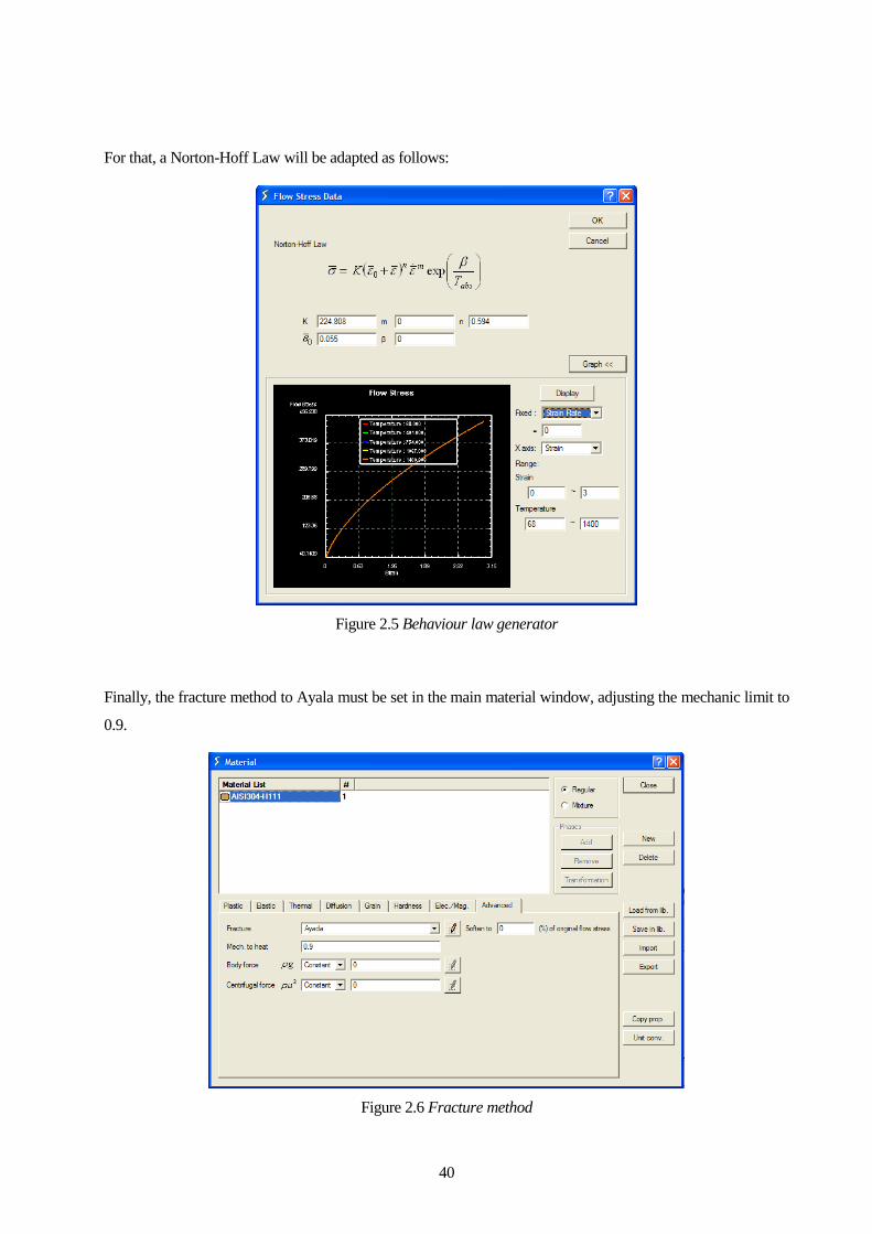
For that, a Norton-Hoff Law will be adapted as follows:

Figure 2.5 Behaviour law generator

Finally, the fracture method to Ayala must be set in the main material window, adjusting the mechanic limit to

0.9.

Figure 2.6 Fracture method

41

Once the material is created, next step is to create the different pieces of the simulation. For the metal sheet,

the elasto-plastic option will be chosen, and in the material option, the AISI304 previously created will be set:

Figure 2.7 Object type and material choosing

Then the geometries for the sheet and the tool will be created. Note that there is no blank holder. That’s

because with blank holder, the program has problems with the boundary conditions (as it will be discussed

later).

To create the geometries, the Geo Primitive option will be selected, and the values will be introduced in mm in

the subsequent window.

Figure 2.8 Geometry selection

42

Figure 2.9 Sheet geometry data

Figure 2.10 Tool geometry data

Then it is needed to adjust the position of the different pieces to locate them properly and generate the

interactions between them with the object positioning option in the main toolbar.


43

As both pieces overlap each other, they need to be separated a bit, and after that make them interfere. For that

first will be used the drag option, that allows moving the object in any direction. In this case the tool will be

moved in the Z direction:

Figure 2.12 Pre-processor drag control

After that, the option interference is used to bring them closer and make them coincide in one point. Notice

that the drop option could be used too, but for this project was used interference so that the rotation of the tool

doesn’t affect (although it wouldn’t affect anyways, because it’s a solid of revolution).

Figure 2.13 Pre-processor interference control

44

With all set, the final geometry is as follows:

Figure 2.14 Simulation geometry correctly positioned

With the geometry set, the meshing will be created. The Automatic Mesh Generator distributes the mesh to

adjust it to the geometry and different conditions predefined by the user, such as mesh windows. It also allows

to automatically remesh when the elements are distorted in a certain percentage or predetermined value.

For this simulation, around 50000 elements are required, giving good results without making the computing

times too long. After trying different number of elements, it is concluded that the Automatic Mesh Generator

adjust the number of elements (and the elements themselves) to the predefined conditions, creating around 1/3

of the total elements required. That’s why the program was set to create a mesh with 150000 elements:

Figure 2.15 Sheet meshing

45

DEFORM™-3D allows to choose between two types of elements: brick, with 8 nodes and tetrahedral, with 4

nodes. However, once the elasto-plastic option is chosen, it is only allowed the tetrahedral ones.

Given the final geometry of the sheet, it is necessary to refine the mesh in the areas close to the centre of the

piece. For that, detailed settings must be clicked, where it can be configured. First the weighting factors have

to be adjusted, making the mesh density window the main one, giving it a value of 1.

Figure 2.16 Detailed meshing settings

After that, mesh windows will be created. In this case, 2 different mesh windows were set: the inner one with a

size ratio of 0.12 (being the most deformed part, a thinner mesh is needed), and the outer one with a size ratio

of 0.25. That sizes, along with the number of elements have proven to be enough to provide good results,

without long computing times.

Figure 2.17 Different meshing windows

46

Now the only thing remaining is simply clicking the Generate Mesh button on the main meshing window

(Figure 2.15). It must be noted that DEFORM™-3D sometimes has a problem with the meshing, where

despite having given the program different mesh windows, it doesn’t use them, generating an uniform mesh:

Figure 2.18 Problem with the meshing

This has a very simple solution: the simulation setting will continue with this mesh, and after the work with the

pre-processor is finished, the program will be set to run a few steps, stopping the program after that, and

manually remesh again in the pre-processor (as the mesh windows are already defined, it is enough with just

clicking the generate mesh button). With that done, the meshing result is as follows:

Figure 2.19 Final meshing for the 20mm tool

47

As it can be seen, with the remeshig, DEFORM™-3D often loses some material from the geometry. In this

study it isn’t considered, as they are minimal loses, and they are located away from the studied zone.

Sometimes during the simulation, the mesh were too much distorted, generating folding problems and being

necessary to stop the simulation, and to remesh manually as it was explained before. In those cases, the new

start point of the simulation was set at a previous step before the occurrence of the above mentioned issue.

With the mesh created, the boundary conditions on the sheet can be set. As told before, this model does not

have a blank holder piece, therefore a substitute boundary condition is needed. That’s because with the blank

holder piece, when the simulation has achieved a noticeable depth, due to numeric errors, part of the sheet gets

inside the blank holder (Figure 2.20), creating contact problems and invalidating the strain and stress values

from that point.

Figure 2.20 Simulation failure with the blank holder

To adjust the model to the experimental analysis, different boundary conditions will be set to embed the

vertical planes of the sheet, and constraint the vertical movement of the sheet there where the blank holder

would be.

For that, the Bdry. Cnd. tab must be clicked, and set three different boundary conditions, one on each axis (x,

y, and z). For that, it will be used the velocity condition, setting it to a value of 0. For the x, y directions, it’s

only needed to set the condition on the nodes of the vertical planes. For the vertical direction, a similar tool as

when setting the mesh windows will be used. In this case, it will be set with an outer radius enough to cover

the entire sheet, and an inner radius of 42mm. That value is to adapt the condition of the experimental blank

holder, which had an inner radius of 40mm, and a 2mm rounded edge. This solution, although it can’t exactly

describe the movement around the blank holder, gives good enough results.

48

(a) (b)

Figure 2.21 Boundary conditions in x and y directions (a) and in z direction (b)

Now the movement of the tool will be set. As said previously, in SPIF processes, the tool moves along a

trajectory generated in a CNC machine, incrementally forming the sheet to achieve the final geometry. Given

the fact that our main goal is to compare the results of this simulation with the experimental, the simulation

parameters will be the same from the experimentation.

However, there is a difference, because the tool doesn’t rotate on itself. The rest of the parameters are indeed

equal, setting the feed rate of 3000mm/min, and a step down of 0.5mm. This step down is used in 2.5 axis

CNC machines that are only capable of interpolate trajectories in one of the 3 main planes (being in this case

the horizontal one), and make linear movements in the remaining axis. If there is a complex geometry, it will

be discretized in several planes. If the machine was 3-axial, the trajectory would describe a 3-dimensional

geometry, without discretization in planes.

Figure 2.22 Tool trajectory with the step down

In order to create the points of the trajectory, PHYTON™ interface was used, that generated all the points

where the tool would move, after introducing the step down, the tool radius, the feed rate, if the free

rotation of the tool is permitted, the direction of rotation (-1 if constant, 1 if alternate, that was our case),

and if there is a pyramidal or conical geometry.

49

To introduce that trajectory in DEFORM™-3D, the tool will be selected in the object tree, and in the

movement tab, the Path option will be selected. Given that the feed rate is known, as also the points of the

trajectory, the function will be defined as Profile+feed rate:

Figure 2.23 Movement window in the pre-processor

After that, it’s needed to click in define function and introduce the x, y, z coordinates of all the points, and the

feed rate, as a table, to obtain the following:

Figure 2.24 Point cloud of the trajectory

50

Now the interactions between the two pieces will be set. For that, the inter object option will be clicked on the

main toolbar:


In the window that will open, the master and slave pieces must be selected. In this case, the sheet is formed by

the tool, so the tool is the master and the sheet the slave. The friction value is introduced here, value that was

estimated of 0.01 of Coulomb friction, that suits better the condition on a lubricated forming such as ours.

Sometimes, despite creating the interaction, the program has problems obtaining the contact conditions. That

problem doesn’t affect the simulation, because when the tool starts forming the sheet (some steps after the

beginning of the simulation), it is correctly detected.

Figure 2.26 Inter object and friction window

To finish with the pre-processor, the simulation parameters will be set in Simulation Controls. As said before,

units are in SI (being length in mm and the stresses in MPa).

In order to calculate the approximate number of steps necessaries for the simulation, the real time of the

process was divided by the step increment control (that was set of 0.005sec/stem), obtaining around 22000

steps. Choosing a right number of steps is very important, because that’s what DEFORM™-3D uses to

calculate. If too few steps are chosen, the simulation may end before the tool finishes forming the workpiece.

51

Figure 2.27 Step number selection

Figure 2.28 Step increment control number selection

With all set, and before starting the simulation, it is needed to check and generate an initial database:


52

Figure 2.30 Database checking and generation

Once the database is generated, the pre-processor can be closed and start the simulation by clicking in the run

button.

DEFORM™-3D has an option of controlling the forming process during the simulation, allowing to modify it

in the middle, or starting again as long as there isn’t a conceptual error, such as a wrong introduced data.

Now, it will be shown the analysis of results obtained at real failure depths: 24.5 mm for the 20 mm tool, and

28 mm for the 10 mm tool.

53

3 RESULTS

With the DEFORM™-3D numeric tool, it was possible to predict the material flux, in both cases, with the 20

and 10 mm diameter tools.

As said before, the main objective on this project is to validate the model in terms of strains, comparing them

with the experimental processes. The principal strains analysis will consist in the search of the values

distribution, and the locations where they are higher. It will be done just in the instant in which the tool

displacement reaches vertically the experimental failure depth.

3.1 20 mm diameter tool

The numeric results bear out the experimental ones. The major strain 𝜀1, is inside the obtained values, with

zones in which its value is around 0.9, as shown in Figure 3.1 in the red shaded areas. As can be seen, those

areas are placed in the higher displacement areas, being there where the fracture would locate.

Figure 3.1 Mayor strain distribution in the outer surface of a SPIF formed AISI304 sheet with a 20 mm

diameter tool

54

If a dot line is set in the outer surface of the sheet, the following strain curve is obtained. The position of the

line was arbitrarily set on the origin YZ plane, and that’s why the results doesn’t reach the maximum value of

𝜀1 = 0.842 obtained in the fracture points.

Figure 3.2 Mayor strain distribution along a dot line in the outer surface of a SPIF formed AISI304 sheet with

a 20 mm diameter tool

Regarding the minor strain, 𝜀2, it can be seen that its value remains between 0.15 and 0.2 in the formed zone,

that matches the experimental results. However, it can be seen a zone where its value rises to around 0.8,

specifically the area where the forming tool executes the step down. That doesn’t correspond with the

experimentation, and it’s probably due to numeric errors during each step down. Since experimentation shows

that the fracture doesn’t occur in that area, we will obviate the results on the step down zone.

55


diameter tool

Figure 3.4 Minor strain distribution along a dot line in the outer surface of a SPIF formed AISI304 sheet with


56

To compare the experimental results, and the numeric ones obtained in DEFORM™-3D, they will be

represented together in the same graph, as follows:

Figure 3.5 Experimental and numeric results of the formability until fracture of a SPIF formed AISI304

sheet with a 20 mm diameter tool

The numeric points in the graph have been obtained by selecting points from several dot lines as the one

shown in Figure 3.2 and Figure 3.4, each line with a different orientation in order to get points from all the

geometry. It can be seen that the results from the simulation resemble the experimental ones almost exactly,

although some points are slightly displaced to the left under the FLC curve. Regardless this small distortion

from the experimental results, the numeric ones accomplish stable plastic deformation above the FLC curve,

following the experimental analysis.

Notice that in the simulation, the mayor strain doesn’t reach the experimental fracture values. That’s because

in the experimental process a necking appeared, increasing the value of the major strain. Since DEFORM™-

3D can’t predict the necking development, its results only adapt the pre-necking experimental results.

Since several remesh steps were needed in order to complete the simulation, it’s worth to evaluate the

evolution of some parameters in each remesh, such as the mesh volume, and the computing time required. The

simulation was performed on a computer with Windows XP, and Intel® i7 920 processor working with 1 core.

Results are shown in Table 3-1:

57

Table 3-1 Parameters of interest during different remeshings

Mesh Total number

of elements

Total steps

performed

Simulation time

between meshings

(approx.)

Mesh volume

(mm3)

% volume

variation from

initial

Initial mesh 50872 3 <1 min 8000.05 0

Remeshing 1 54206 17000 72 hrs 7993.72 -0.07912451

Remeshing 2 46992 19200 10 hrs 8147.54 1.84361348

Remeshing 3 44033 19375 1 hr 8187.91 2.34823532

Remeshing 4 43768 19400 10 min 8184.63 2.30723558

Remeshing 5 44651 19605 1 hr 8182.38 2.27911076

Remeshing 6 44842 19700 30 min 8179.74 2.24611096

As shown in the table, as the simulation goes further, more frequent remeshings are needed. That’s because of

the final frustum geometry, meaning that the deeper the tool is, the faster it deepens, because the curve gets

smaller in each step down, distorting the mesh faster.

The simulation time is highly estimated, firstly because of the impossibility of the author of this project to be

always controlling the simulation, and secondly because in order to realize the necessity of a remeshing, it was

needed the simulation to run some steps more, to notice the failure, and then remesh several steps before the

failure (in this project, the remeshings were done about 100 steps before the failure step every time it was

possible), roughly extending the total simulation time (from the initial meshing to the end of the simulation) to

5 days or a week.

As can be seen, the mesh volume slightly increases during the simulation. This is due to numeric errors in the

nodes of the mesh, but since the total variation is smaller than a 5%, it isn’t considered.

58

3.2 10 mm diameter tool

The process with the 10 mm diameter tool presents a slightly worse geometry, caused by numerical errors

because of the indentation of the tool. This means that DEFORM™-3D can’t predict the material flux in the

10 mm tool process as well as in the 20 mm one. However, the obtained results in both cases still are

acceptable.

Figure 3.6 Final geometry of a SPIF formed AISI304 sheet with a 20 mm diameter tool

Figure 3.7 Final geometry of a SPIF formed AISI304 sheet with a 10 mm diameter tool

In this case the same procedure will be used, analysing each strain separately, to finally create the FLD graph

with both the experimental and numerical results. Again, the numeric results adjust with the experimental

analysis, with a highest value of the major strain of 𝜀1 = 1.28, located again in the higher displacement areas.

59

Figure 3.8 Mayor strain distribution in the outer surface of a SPIF formed AISI304 sheet with a 10 mm

diameter tool

Figure 3.9 Mayor strain distribution along a dot line in the outer surface of a SPIF formed AISI304 sheet with


60

Again, the minor strain values correspond with the experimental results in all the geometry but the step down

area, which again has values of about 0.7 due to numeric errors, which will be obviated.


diameter tool

Figure 3.11 Minor strain distribution along a dot line in the outer surface of a SPIF formed AISI304 sheet with


61

Figure 3.12 Experimental and numeric results of the formability until fracture of a SPIF formed AISI304


Again, representing the experimental and the numeric results in the same graph, allows to compare them.

Similar to the 20 mm tool case, here can be seen that the results from the simulation resemble the experimental

ones, being slightly displaced to the right.

Since the experimental analysis of the 10 mm tool process proved that there were a much smaller necking

within the failure of the sheet than in the 20 mm tool process, in this case the simulation can adjust and predict

almost perfectly the final failure strains. That, allows again stable plastic deformation above the FLC curve,

and specifically in this case, allowing the principal strains to reach and slightly overpass the FFL curve within

stable deformation.

62

3.3 Accumulated damage

In metal forming it’s basic to prevent the fracture failure, depending for that of a strain limit study, as the one

that has been realised in this project. By calculating the accumulated damage, it will be possible to calculate

when and where the fracture will appear, with the calculated strains and stresses.

DEFORM™-3D uses the Normalized Crockroft & Latham as default damage model, but allows to choose

between other damage models, listed here:

Normalized C&L

Cockroft & Latham

McClintock

Freudenthal

Rice & Tracy

Oyane

Oyane (negative)

Ayada

Ayada (negative)

Osakada

Brozzo

Zhoa &Kuhn

Maximum principal stress / ultimate tensile strength

User routine

In this project, the Ayada damage model was used:

𝐷 = ∫𝜎𝐻

�̅�dε̅

�̅�𝑓

0

Where D is the accumulated damage, ε̅ and �̅� are equivalent strains and stresses, 𝜎𝐻 the hydrostatic stresses

and 𝜎1 the major principal stress. When introducing any damage model in DEFORM™-3D, a critical value is

needed, that will be calculated later.

According to fracture mechanics, fracture failure on metal forming has 3 different modes of fracture. The

ductile fracture criterion used in this project is based in Mode I.

Figure 3.13 Fracture modes; respectively, Mode I, Mode II, and Mode III

63

The circumstances where each fracture mode occurs are identified in terms of microstructural ductile damage

and plastic flux. In SPIF, the plastic material flux and the failure is a combination of modes I and II, while in

traditional forming methods it’s a combination of modes I and III.

With analytic calculus, it’s possible to characterize the fracture mode in terms of stress conditions. To study it,

Atkins & Mai (1985) established a relationship among the inclusions space, the holes diameter and the triaxial

stress state at the onset of the crack propagation.

Figure 3.14 Crack propagation in fracture Mode I

Results of the analysis, proved that the critical damage was as follows:

𝐷𝑐𝑟𝑖𝑡 = ∫𝜎𝐻

�̅� dε̅

�̅�

0

That equation, developed under Hill’s anisotropic plasticity criterion, with plane stress conditions, gives, as

exposed on Silva et al (2008-09-11):

𝐷𝑐𝑟𝑖𝑡 =(1 + 𝑟)

3(𝜀1𝑓 + 𝜀2𝑓)

As in this project it has been assumed the isotropy of the material, r is determined and equal to 1; and 𝜀1𝑓 and

𝜀2𝑓 are respectively the mayor and minor strains on the fracture point. This allows to conclude that the tensile

fracture limit in Mode I is independent of the strain path and equivalent to the critical thickness reduction.

Therefore, with this results it’s possible to check if the accumulated damage in the simulation corresponds the

critical damage obtained in the experimentation, when ductile fracture appears. The integral equation will be

used to calculate the accumulated damage on the simulation until experimental failure strains are reached, and

the discrete one will allow to obtain the critical damage with the values of r and the mayor and minor fracture

strains of the experimental tests.

Thus, it will be possible to predict if the simulation reached the critical damage, knowing that the area where it

is reached will be where the fracture would occur. That doesn’t mean that it will always happen in the same

point, but it bears out if it will happen when the experimental depth is reached.

64

With the strains results obtained by Centeno et al (2014), the experimental critical damage values are:

Table 3-2 Strain fracture and experimental critical damage values

𝜺𝟏𝒇 𝜺𝟐𝒇 𝑫𝒄𝒓𝒊𝒕 =𝟐

𝟑(𝜺𝟏𝒇 + 𝜺𝟐𝒇)

20 mm diameter tool 0.95 0.15 0.733

10 mm diameter tool 1.1 0.1 0.8

3.3.1 20 mm diameter tool

Figure 3.15 Distribution of the accumulated damage according the Ayada criterion on a SPIF formed AISI304


As can be seen, although in the simulation the accumulated damage is slightly higher than the experimental

one, it fits quite well in areas of maximum mayor strain, being most of those areas with values around 0.5, and

some punctual zones where it reaches the critical value (small orange/red dots).

65

3.3.2 10 mm diameter tool

Figure 3.16 Distribution of the accumulated damage according the Ayada criterion on a SPIF formed AISI304


Similar to the 20 mm tool diameter case, the accumulated damage is slightly higher in this simulation than the

experimental critical damage, fitting the experimental results with acceptable accuracy in areas of maximum

mayor strain.

67

4 CONCLUSIONS AND FUTURE

DEVELOPMENTS

4.1 Conclusions

In this project was created a Finite Element Method model in DEFORM™-3D, for 0.8 mm thickness

AISI304-H111 sheets, in order to analyse the strain state during the process. After comparing the simulation

results with the experimental ones obtained by Centeno et al. (2014), it was proved that they fit quite well to

the experimentation, allowing to validate the numeric model.

Because of the long computing times, several simplifying assumptions were made in the model, such as

considering the material as isotropic, and setting the boundary conditions as embeddings in the vertical planes

of the sheet. Although it wasn’t to reduce the computing time, it’s worthy to mention the vertical condition that

replaces the blank holder to solve the numeric problems commented.

Those simplifications might affect the small differences between the numeric and the experimental results, but

they were done to reduce computing times, but still provide results that followed acceptably the ones from the

real process.

Thus, the simulations where accomplished, following the same parameters as the experimental tests. There

were performed with 20 mm and 10 mm diameter tools, and the step down was set to 0.5 mm. Therefore, not

all the experimental tests where simulated (since in the experimentation, tests were performed with 0.2 mm

step down, too), but given that the results for each step down proved to be very similar, it wasn’t necessary. In

both simulations, the principal strain levels at the real failure depth where similar to the experimental ones.

Principal strains from the simulations were compared with the experimental results in the Forming Limit

Diagram, for each case.

Critical damage levels were also analysed, comparing the critical damage obtained in the experimentation with

the values provided by the Ayada criterion in the simulation, at the real failure depth. In both cases, 10 mm and

20 mm diameter tools, the obtained values were very close to the experimental, proving that the Ayada

criterion allows to properly predict plastic failure in this simulations.

Finally, with the simulations concluded and analysed, a step by step manual was created to easily show how to

model the incremental forming processes carried out in this project, using DEFORM™-3D.

68

4.2 Future developments

Once the model is validated, it could be extrapolated to other tool diameters, such as 8 mm, 12 mm, etc., or

trying to determine the smallest diameter for which DEFORM™-3D can’t correctly predict the material flux.

Other parameters could be numerically analysed, such as the influence of the feed rate, the friction, the tool

rotation or the element size, creating different meshes, or variating the mesh size on the remeshes.

Another Finite Element Method softwares could be used, implementing models in both explicit calculation

based models such as LS-Dyna®, and implicit ones as Abaqus®, to be able to compare which program gives

better results in simulated SPIF processes.

Finally, it could also be extended to other industrial application variants of SPIF with different geometries,

such as hole flanging processes.

69

REFERENCES

Amino, H. et al., 2002. Dieless NC Forming, Prototype of automotive Servive Parts Proceedings of the 2nd

International Conference on Rapid Prototyping and Manufacturing (ICRPM).

Aoyama, S., Amino, H., Lu Y. & Matsubara, S., 2000. Apparatus for dieless forming plate materials.

Europe, Patent No. EP0970764.

Candel, Z. Análisis numérico de la conformabilidad de chapas de AA2024-T3 en procesos de conformado

incremental mono-punto usando DEFORM-3D. Trabajo de Fin de Grado. University of Seville.

Carmona, J. Numerical Analysis on DEFORM-3D of limit strains in Single Point Incremental Forming for

AISI304-H111 sheets. Proyecto de Fin de Carrera. University of Seville.

Centeno,G. et al., 2011. Experimental Study on the Overall Spifability of AISI 304. Sevilla-Girona, University

of Sevilla & University of Girona, p. 8.

Centeno, G. et al., 2012. FEA of the Bending Effect in the Formability of Metal Sheets via Incremental

Forming, Steel Research International. pp 447-450.

Centeno, G. et al., 2012. Experimental Study on the Evaluation of Necking and Fracture MESIC, p.8.

Centeno, G. et al., 2014. Critical analysis of necking and fracture limit strains and forming forces in single-

point incremental forming Materials and design, Volume 63 pp.20-29.

Emmens W. & Van den Boogaard, A., 2009. An overview of stabilizing deformation mechanism

incremental sheet forming, Journal of Material processing Technology , Volume 211 pp. 3688-3695.

Goodwin, G., 1968. Application of strain analysis to sheet forming problems in the press shop. MET ITAL,

Aug, 60(8), pp. 767-774.

Hirt , G., 2004. Tools and Equipment used in Incremental Forming. Incremental Forming Workshop,

University of Saarbruckewn, June 9. p. 27.

Hirt, G., Ames, J., Bambach, M., & Koop, R., 2004. Forming strategies and Process Modeling for CNC

Incremental Sheet Forming. January, Volume 53, p. 203.

70

ISO, 2008. 12004-2:2008. Metallic materials -- Sheet and strip -- Determination of forming-limit curves --

Part 2: Determination of formig-limit curves in the laboratory.

Jeswiet, J., Duflou, J., Szekeres, A. & Levebre, P., 2005. Custom Manufacture of a Solar Cooker - a case

study. Journal Advanced Material Research, May. Volume 6-8.

Jeswiet, J., et al. 2010. Asymmetry Single Point Incremental Forming of Sheet Metal.

Keeler, S., 1965. Determination of forming limits in automotive stampings. SHEET METAL IND, Sep,

42(461), pp. 683-691.

Leszak, E., 1967. Apparatus and Process for Incremental Dieless Forming., Patent No. US3342051A1.

Marciniak, Z., Duncan, J. & Hu, S., 2002. Mechanics of Sheet Metal Forming. London Butterworth-

Heinenrmann.

Meier, H., Dewald, O. & J., Z., 2005. Development of a Robot-Based Sheet Metal Forming Process. In steel

research, Volume 1.

Powell, N. & Andrew, C., 1992. Incremental forming of flanged sheet metal components without dedicated

dies. IMECHE part B, J. of Engineering Manufacture, Volume 206.

Ruiz, F. Análisis numérico de procesos de conformado incremental monopunto en chapas de aluminio

AA7075-T3. Trabajo de Fin de Grado. University of Seville.

Schafer, T. & Schraft, R. D., 2004. Incremental sheet forming by industrial robots using a hammering tool.

AFPR Association Francais de Prototypag Rapid, 10th European Forum on Rapid Prototyping, 14 Sep.

Schmoeckel, D., 1992. Developments in Automation, Flexibilization and Control of Forming Machinery.

Anuals of CIRPM, Volume 40/2, p. 615.

Silva, M., Nielsen, P., Bay, N. & Martins, P., 2011. Failure mechanims in single-point incremental forming

of metals. 1 March.

Silva, M., Skjoedt, M., Bay, N. & Martins, P. & Bay, N., 2008. Revisiting single-point incremental forming

and formability/failure diagrams by means of finite elements and experimentation. International Journal of

Machine Tools & Manufacture, Issue 48, pp. 73-83.

Silva, M., Skjoedt, M., Martins, P. & Bay, N., 2007. Revisiting the fundamentals of single point incremental

forming by means of membrane analysis. International Journal of Machine Tools & Manufacture, Issue 48,

pp-3-5.

71

Skjoedt M., Bay N., Endelt B. and Ingarrao G., 2008. Multi-stage strategies for single point incremental

forming of a cup. 11th ESAFORM conference on metal forming – ESAFORM2008.

Stewart, D., 2005. A Platform with Six Degrees of Freedom. UK Institution of Mechanical Engineers

Proceedings, 180 (15).

Suntaxi, C., 2013. Análisis experimental de deformaciones límite en chapas de acero AISI 304 en

conformado incremental. Trabajo de Fin de Máster. Universidad de Sevilla.

Análisis numérico en DEFORM-3D de deformaciones

límite en conformado incremental mono-punto de

chapas de acero AISI304-H111

Departamento de Ingeniería Mecánica y

Fabricación




Sevilla, 2016

Resumen Trabajo Fin de Grado


Numerical Analysis on DEFORM-3D of limit strains

in Single Point Incremental Forming for AISI304-

H111 sheets



1

1 INTRODUCCIÓN

El conformado de chapas metálicas en la industria actual es un proceso de amplia utilización en un

gran número de sectores de producción, estando por tanto en continuo progreso y revisión.

Por ejemplo, en el sector aeronáutico, el estirado de chapa se usa para crear las piezas del fuselaje,

siendo necesarios un equipamiento y herramientas muy especializados. Es por esto que esta tecnología

solo es rentable a gran escala.

El conformado incremental de chapa (Incremental Sheet Forming, ISF) es un proceso innovador que

cumple los requerimientos de flexibilidad, sostenibilidad y coste de las tecnologías de fabricación

actuales, en el que no es necesario el uso de maquinaria y equipamiento dedicados, haciendo que sea

viable para lotes pequeños y medios.

El conformado incremental mono-punto (Single Point Incremental Forming, SPIF) es el proceso de

fabricación más simple entre los basados en el conformado incremental. Consiste en una herramienta

hemisférica controlada por una máquina de control numérico (CNC) que sigue progresivamente una

trayectoria preestablecida, deformando plásticamente una chapa metálica para obtener distintas

geometrías sin necesidad de troquel. Esto permite un aumento en la conformabilidad, además de las

otras ventajas mencionadas previamente.

En este proyecto se calculará numéricamente la evolución de deformaciones en una chapa de acero

AISI304-H111 para herramientas de 100 mm y 20 mm de diámetro, con un programa basado en el

método de los elementos finitos (FEM), el DEFORM™-3D. Esto, bajo ciertas hipótesis, permitirá

tener un modelo para comparar los resultados experimentales obtenidos por Centeno et al (2014), así

como permitir obtener la evolución de tensiones en la chapa.

1.1 Antecedentes

El aumento de la conformabilidad de chapas metálicas por medio de procesos de conformado

incremental, específicamente de conformado incremental mono-punto, ha sido experimentalmente

estudiado por varios autores, como Emmens et al (2009), Jeswiet et al (2010) o Silva et al (2011),

entre otros.

El grupo de investigación de Ingeniería de los Procesos de Fabricación de la Escuela de Ingeniería de

la Universidad de Sevilla del Departamento de Ingeniería Mecánica ha realizado numerosos ensayos

2

tanto experimentales como simulaciones numéricas sobre el conformado de chapas metálicas

sometidas a SPIF, especialmente la influencia de la flexión en los procesos de conformado, evaluando

los mecanismos de fallo e investigando qué parámetros les afectan, como hicieron en Centeno et al

(2012).

Bajo esa línea de investigación, se ha desarrollado una metodología para obtener los diagramas límite

de conformado (Forming Limit Diagram, FLD), tanto para situaciones de estirado como de estirado

con flexión. Esta metodología ha sido probada para diversos materiales, como los aluminios AA7075-

O, AA2024-T3, o el acero AISI304-H111, entre otros.

Este último material será el que se analizará en este proyecto. En Centeno et al (2014), se obtuvo la

siguiente evolución de deformaciones en SPIF, en la cara externa de una chapa de acero AISI304, una

vez ocurrió el fallo:

Figura 1.1 Resultados experimentales para una chapa AISI304-H111 conformada por SPIF con

herramientas de 20 mm y 10 mm de diámetro, y steps down de 0.2 mm y 0.5 mm por pasada

Se llevaron a cabo varios ensayos distintos, con herramientas 6 mm, 10 mm, y 20 mm de diámetro.

Para cada herramienta, el step down se ajustó alternativamente a 0.2 mm y 0.5 mm por pasada. Tres

ensayos iguales se realizaron para cada uno de los casos, obteniéndose prácticamente los mismos

resultados en ellos.

El estado final de deformaciones fue medido con el programa ARGUS®, y las deformaciones de

fractura fueron obtenidas midiendo los espesores de la chapa a lo largo de la grieta, a ambos lados de

ésta.

3

Figura 1.2 Fractografía de la zona de fallo en el proceso de estirado con flexión (stretch-bending)

usando un punzón cilíndrico de 20 mm de diámetro (izquierda), y de 10 mm (derecha).

Figura 1.3 (a) Esquema de la geometría usada en el SPIF, (b) patrón de puntos en la geometría final

(c) resultados de la deformación principal 𝜀1 obtenidos con el programa ARGUS® y (d) corte de la

geometría final listo para medir los espesores a lo largo de la grieta.

Como se puede ver en la Figura 1.1, hay un gran aumento en la conformabilidad de las chapas de

acero AISI304-H111, permitiendo una deformación plástica estable hasta valores de deformación

principal 𝜀1 muy por encima de la curva límite de conformado (Forming Limit Curve, FLC), donde

normalmente comienza a haber estricción, y cercanos a la curva de fractura (Fracture Forming Line,

FFL). Especialmente, en el caso de la herramienta de 10 mm de diámetro, las deformaciones

principales alcanzan la FFL manteniendo una deformación estable. En ese caso, la deformación

principal 𝜀1 alcanza valores de hasta 1.1 en escala logarítmica de deformaciones, ubicándose

ligeramente por encima de la curva FFL obtenida en los ensayos de estirado de Nakazima.

5

2 DEFORM™-3D

En este apartado se comentarán brevemente los pasos clave necesarios para crear el modelo de

DEFORM™-3D para los análisis pedidos. Para una guía más detallada, ver el documento original en

inglés.

DEFORM™-3D es un sistema procesador de simulaciones que analiza el flujo tridimensional en

conformado de metales. Proporciona los flujos de material sin los costes y retrasos derivados del

análisis experimental, y ha demostrado ser una solución robusta en el entorno industrial durante más

de dos décadas.

DEFORM™-3D permite importar geometrías desde CATIA, y su programa FEM que tiene integrado

permite predecir la fractura en múltiples procesos, como mecanizado, estampación, extrusión,

laminado, etc.

El generador de malla automático (AMG) genera y optimiza la malla allí donde es necesario. También

tiene un sistema user-defined, que permite al usuario especificar la densidad de la malla donde

convenga. También permite parar la simulación, volver a un paso anterior y modificar los parámetros

ahí, permitiendo retomar la simulación desde ese punto. Esta es una de las principales ventajas de

DEFORM™-3D en comparación con otros programas FEM, y se utilizará varias veces en este

proyecto, ya que a ciertas profundidades la malla se deformará y será necesario remallar manualmente.

2.1 DEFORM™-3D como herramienta numérica

El modelo se creará en el pre-processor del programa, siendo necesario primero crear el material y las

piezas. Para ello, vamos a la barra principal del pre-processor:

Figura 2.1 Barra principal del pre-processor, respectivamente los botones de Simulation Controls,

Material, Object Positioning, Inter Object y Database Generation.

6

En la opción Material es posible crear un nuevo material o modificar uno ya existente. En este caso

se modificará el existente en la base de datos, con una ley de comportamiento plástico de Norton-

Hoff, que permite adaptar la ley de Schwift obtenida por Centeno et al (2014).

Figura 2.2 Generador de la ley de comportamiento

A continuación se crean las piezas. Para la chapa metálica, se selecciona la opción elasto-plástico en

la ventana principal del pre-processor, y se le establece el material previamente creado.

Para las geometrías, se seleccionará la opción Geo Primitive, y se introducirán los datos en mm en la

ventada subsiguiente. Nótese que el programa tiene que estar configurado en SI en la ventana de

Simulation Controls.

Figura 2.3 Geometrías de la chapa y el punzón

Una vez generadas las piezas, hay que ajustar las posiciones relativas de las piezas con la ventana

Object Positioning en la barra principal para ubicarlas correctamente.

A continuación se creará la malla de la chapa. Para ello se establecerán 150000 elementos, obteniendo

finalmente en torno a 50000 (se comprobó que el generador de malla automático reduce los elementos

totales a 1/3). Dada la geometría final de la chapa, es necesario refinar la malla en algunas zonas. Para

ello, en la pestaña Detailed Settings, se establecerá el valor máximo para la opción Mesh Density

Windows en la pestaña Weighting Factors.

7

Figura 2.4 Ventana de mallado de la chapa

Una vez hecho esto, se crearán dos ventanas de mallado: la interna tendrá un size ratio de 0.12 (al ser

la zona más deformada, necesita una malla más fina) y la externa con un ratio de 0.25. Estos valores

han demostrado dar resultados aceptables sin grandes tiempos de computación.

Una vez se ha generado la malla, DEFORM™-3D puede dar un fallo en el que las ventanas de mallado

no aparecen, siendo una malla uniforme. La solución a esto es sencilla, una vez finalizado el modelo,

dejar avanzar el programa unos pasos y remallar manualmente (dado que las ventanas de mallado ya

están establecidas, bastará con hacer click en la opción Generate Mesh).

Como se ha comentado previamente, a veces en la simulación la malla estaba demasiado

distorsionada, generando problemas de folding, haciendo necesario parar la simulación y remallar

manualmente de nuevo. En esos casos, el nuevo punto de comienzo se estableció en un paso previo a

la aparición del mencionado fallo.

Figura 2.5 Problema con el mallado (izda) y malla final (dcha)

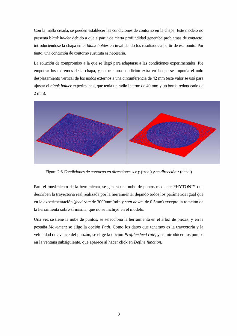
8

Con la malla creada, se pueden establecer las condiciones de contorno en la chapa. Este modelo no

presenta blank holder debido a que a partir de cierta profundidad generaba problemas de contacto,

introduciéndose la chapa en el blank holder en invalidando los resultados a partir de ese punto. Por

tanto, una condición de contorno sustituta es necesaria.

La solución de compromiso a la que se llegó para adaptarse a las condiciones experimentales, fue

empotrar los extremos de la chapa, y colocar una condición extra en la que se imponía el nulo

desplazamiento vertical de los nodos externos a una circunferencia de 42 mm (este valor se usó para

ajustar el blank holder experimental, que tenía un radio interno de 40 mm y un borde redondeado de

2 mm).

Figure 2.6 Condiciones de contorno en direcciones x e y (izda.) y en dirección z (dcha.)

Para el movimiento de la herramienta, se genera una nube de puntos mediante PHYTON™ que

describen la trayectoria real realizada por la herramienta, dejando todos los parámetros igual que

en la experimentación (feed rate de 3000mm/min y step down de 0.5mm) excepto la rotación de

la herramienta sobre sí misma, que no se incluyó en el modelo.

Una vez se tiene la nube de puntos, se selecciona la herramienta en el árbol de piezas, y en la

pestaña Movement se elige la opción Path. Como los datos que tenemos es la trayectoria y la

velocidad de avance del punzón, se elige la opción Profile+feed rate, y se introducen los puntos

en la ventana subsiguiente, que aparece al hacer click en Define function.

9

Figura 2.7 Nube de puntos de la trayectoria

A continuación se selecciona el Inter-Object para establecer la relación entre las piezas, siendo la pieza

maestra la herramienta y la esclava la chapa. Con esto seleccionado, queda por establecer la fricción

con un valor de 0.01 de Coulomb y generar la relación.

Finalmente, se establecen el número de pasos necesarios en la ventana de Simulation Controls,

calculados dividiendo el tiempo real entre el step increment control (que se estableció en 0.005 s/paso)

obteniendo unos 22000 pasos.

Antes de iniciar la simulación, se tiene que generar una base de datos, que requiere ser comprobada

primero, ambas opciones ubicadas en la ventana que se abre al clickar en Database Generation:

Figura 2.8 Generación de la base de datos

10

Con la base de datos creada, basta con cerrar el pre-processor e iniciar la simulación haciendo click

en el botón run.en la ventana principal de DEFORM™-3D.

A continuación se exponen brevemente los resultados en términos de deformaciones principales

obtenidos para la herramienta de 20 mm:

Figura 2.9 Distribución de la deformación principal 𝜀1 en la cara contraria a la acción del punzón

de 20 mm de diámetro en una placa de AISI304-H111 conformada por SPIF

Figura 2.10 Distribución de la deformación principal 𝜀2 en la cara contraria a la acción del punzón

de 20 mm de diámetro en una placa de AISI304-H111 conformada por SPIF

11

Estos resultados corroboran lo obtenido experimentalmente, estando los valores de la deformación

principal 𝜀1 dentro del margen obtenido experimentalmente, habiendo zonas con valores en torno a

0.9 (coloreadas en rojo); mientras que para la deformación principal 𝜀2 los valores suelen estar en

torno a 0.15-0.2, con zonas puntuales en torno 0.3.

Conviene mencionar que hay una zona en la que los valores de 𝜀2 aumentan hasta 0.8, en el área donde

la herramienta realiza el step down. Esto no se corresponde con los resultados experimentales, y es

probablemente debido a errores numéricos provocados en cada bajada. Como la experimentación

muestra que la fractura no ocurre en esa zona, se obviarán los resultados de la zona de bajada de la

herramienta.

Por tanto, a la vista de los resultados, se concluye que el modelo es válido, siendo capaz de predecir

aceptablemente los flujos de material, y los resultados en deformaciones y tensiones en toda la

geometría, exceptuando la zona de bajada de la herramienta previamente mencionada.

13

3 CONCLUSIONES

En este proyecto se ha creado un modelo de elementos finitos en DEFORM™-3D, para chapas

metálicas de acero AISI304-H111 de 0.8 mm de espesor, para analizar el estado de deformaciones a

lo largo del proceso. Después de comparar los resultados de la simulación con los experimentales

obtenidos por Centeno et al (2014), se ha probado que la simulación se ajusta a la experimentación,

permitiendo validar el modelo numérico.

Debido a los grandes tiempos de computación, varias hipótesis simplificadoras se aplicaron al modelo,

como considerar el material isótropo, y el empotramiento de los extremos de la placa. También vale

la pena mencionar, aunque no fuese para reducir tiempo de computación, la condición de contorno

vertical que reemplaza el blank holder para solucionar los problemas numéricos comentados.

Esas simplificaciones afectan a las pequeñas diferencias entre los resultados numéricos y los

experimentales, pero se hicieron de manera que los resultados numéricos seguían a los experimentales,

a la vez que reducían tiempo de computación.

Así, las simulaciones se completaron siguiendo los mismos parámetros que los análisis

experimentales. Se llevaron a cabo con herramientas de 20 mm y 10 mm de diámetro, y un step down

de 0.5 mm. Por tanto, no se simularon todos los tests experimentales (ya que también se probó un step

down de 0.2mm en la experimentación), pero dado que los resultados para cada step down demostraron

ser muy similares entre sí, no se ha considerado necesario. En ambas simulaciones, las deformaciones

principales a la profundidad de fallo real fueron muy similares a las experimentales.

Además, una vez acabadas y analizadas las simulaciones, se creó un manual paso a paso para mostrar

fácilmente cómo modelar los procesos de conformado incremental llevados a cabo en este proyecto

con DEFORM™-3D.

Trabajo Fin de Grado Ingeniería Aeroespacial Análisis ...

Documents

Transcript of Trabajo Fin de Grado Ingeniería Aeroespacial Análisis ...