Zernike power spectra of clear and cloudy light-polluted urban night skies

Salvador Bará,1,* Víctor Tilve,2 Miguel Nievas,3 Alejandro Sánchez de Miguel,4 and Jaime Zamorano4

1Área de Óptica, Dept.de Física Aplicada, Fac. de Física, Universidade de Santiago de Compostela, 15782 Santiago de Compostela, Galicia, Spain

2 Astronomical Observatory "R.M. Aller", Dept. of Applied Mathematics, Universidade de Santiago de Compostela, 15782 Santiago de Compostela, Galicia, Spain.

3Dept. de Física Atómica, Molecular y Nuclear, Fac. de Ciencias Físicas, Universidad Complutense, Madrid, Spain 4Dept. de Astrofísica y CC. de la Atmósfera, Fac. de Ciencias Físicas, Universidad Complutense, Madrid, Spain

*Corresponding author: salva.bara@usc.es

Received Month X, XXXX; revised Month X, XXXX; accepted Month X, XXXX; posted Month X, XXXX (Doc. ID XXXXX); published Month X, XXXX

The Zernike power spectra of the all-sky night brightness distributions of clear and cloudy nights are computed using a modal projection approach. The results obtained in the B, V and R Johnson-Cousins' photometric bands during a one-year campaign of observations at a light-polluted urban site show that these spectra can be described by simple power laws with exponents close to −3 for clear nights and −2 for cloudy ones. The second-moment matrices of the Zernike coefficients show relevant correlations between modes. The multiplicative role of the cloud cover, that contributes to a significant increase of the brightness of the urban night sky in comparison with the values obtained in clear nights, is described in the Zernike space. © 2014 Optical Society of America

OCIS codes: (010.1290) Atmospheric optics; (110.0110) Imaging systems; (100.2960) Image analysis http://dx.doi/org/10.1364/AO.99.099999

1.Introduction

The constant increase of the sky glow produced by the anthropogenic emissions of light is one unwanted side-effect of the continuous spread of public and private lighting systems. A considerable amount of research is being devoted to the measurement and characterization of this phenomenon, in order to get reliable data for modeling accurately its propagation [1−6], to understand better its consequences in diverse fields [7−14], and to devise practicable strategies to keep it within acceptable limits [15−16].

The multiplicative role of the cloud cover is also a matter of concern. Clouds greatly enhance the night sky brightness by reflecting (scattering) the upward radiation of the city lights. Urban overcast skies may reach radiances an order of magnitude higher than the corresponding clear skies, and four times bigger than rural clear moonlit nights [17−19]. Overall, the present levels of light pollution in many places across the world amount to a substantial change in the natural conditions of the nighttime environment.

A widespread technique for monitoring the night sky brightness is based on the use of all-sky cameras with hemispheric field-of-view [20−23] that record with good spatial resolution the sky radiance in standard astronomical photometric bands like the B, V, and R Johnson-Cousins' set [24]. In a previous work [25] we have shown that the all-sky night brightness maps obtained in clear and moonless nights can be efficiently described in terms of Zernike polynomials [26−27]. Using this approach the information content of each map is condensed into an equivalent small-sized vector whose elements (the Zernike coefficients) have a definite physical meaning.

Besides achieving a significant level of essentially lossless data compression, the study of the hemispherical night sky brightness may benefit that way from the conceptual and computational tools associated with modal analysis.

As an example of application we described in that work the modal composition of clear and moonless urban night skies in the range of low to mid Zernike frequencies (radial orders 10≤n ). While an expansion up to this order is generally enough for a successful reconstruction of the relatively smooth maps corresponding to clear skies, it falls somewhat short for other practical applications. Cloudy skies, for instance, generally require to be expanded up to higher Zernike orders if one wants to reproduce accurately the irregular radiance distributions associated to the different types of clouds and the varying degrees of cloud coverage. On the other hand, a full statistical description of the ensemble of night sky brightness maps requires the determination of the covariance matrix of the Zernike coefficients as well as the associated noise propagators. For many relevant applications (e.g. evaluating the reconstruction error associated to different estimation algorithms or building the optimum linear minimum mean square error estimators [28]) these matrices have to be determined up to radial orders high enough as to ensure that no significant truncation error remains in the expansion.

In this work we describe the Zernike statistics of the night sky brightness of clear and cloudy urban skies in the B, V, and R Johnson-Cousin's photometric bands. We evaluate their Zernike composition and describe their second-moment statistical parameters with special emphasis on its asymptotic behavior in the region of high Zernike spatial frequencies ( 2711 ≤< n ). To

achieve such high-order modal expansion the definition domain of the Zernike polynomials must be reasonably free from obstacles blocking the hemispheric field of view. In most urban sites this requires setting the limit of the unit-radius circle at some angular height above the geographical horizon. If the unit radius circle is unblocked and the all-sky maps have enough pixels we show here that a modal projection approach can be used as a practical alternative to the conventional least-squares estimation procedure based on the use of pseudoinverse matrices [25, 28−29].

The contents of this paper are as follows: in Section 2 we describe the modal projection approach and its application to the determination of the Zernike coefficients of the night sky up to high radial orders. Section 3 provides expressions to evaluate the expected reconstruction error and derives the associated noise propagators, which account for the effects of the measurement noise onto the final results. Section 4 reports the experimental results obtained from a set of 603 all-sky maps taken at a urban light-polluted site during a one-year observation run carried out by Universidad Complutense of Madrid, including a wide sample of partially cloudy and overcast skies. In Section 5 we analyze the amplification effects of the cloud cover and in Section 6 we explore the possibility of getting statistically reliable information of the night sky brightness outside the region originally used to compute the Zernike coefficients. Additional remarks, including the relationship between the modal projection approach and the conventional least-squares fitting algorithms, can be found in Section 7. Conclusions are summarized in Section 8.

2.High-order Zernike estimation of the night sky brightness by modal projection

"Night sky brightness" is a short-hand term for the spectral radiance of the night sky weighted by the trasmittance function of a given photometric filter and integrated across wavelengths. An all-sky night brightness map is the projection of the hemispheric brightness distribution of the celestial vault onto a flat circular domain. The projections that conserve the surface element are particularly useful for modal analyses. Henceforth we will consider all-sky night brightness maps obtained using a zenithal equal area (ZEA) projection [30].

The actual Zernike coefficients ka (k = 1,...,∞) of an all-sky night brightness map ( )rB are given by:

( ) ( ) = =

=1

0

2

0

dd1

r

kk rrZBaπ

θ

θπ

rr , (1)

where ( )rkZ is the k-th Zernike mode, ( )θ,r=r is the position vector on the map plane, being r the zenital distance and θ the azimuth angle, and the integration is performed over C, the unit-radius circle of area π chosen to define the Zernike polynomials. Eq. (1) is the analytical expression of the modal projection operation whereby each Zernike coefficient is obtained as the inner product of ( )rB and the corresponding element of the basis in the Hilbert space.

Since the experimental all-sky images are pixelated and noise-degraded versions of the sky radiance we do not have access in practice to the actual values of ( )rB , but rather to a discrete set of measurements ( ) ( ) ( )ppp BS rrr ν+= , where ( )pB r (p = 1,..,N) is the actual brightness integrated within the field-of-view of the pixel p, pr is the position vector of the center of that pixel expressed in normalized coordinates in C, and ( )prν is the pixel

noise. N is the number of pixels contained in C. This data set can be arranged for convenience as a ( )1×N column vector such that the above expression can be compactly written as νbs += .

If the number of pixels N of the all-sky map is high and there are no significant obstacles within C blocking the view of the celestial vault, the first M Zernike coefficients of ( )rB can be estimated by evaluating the modal projection integrals in Eq.(1) as discrete sums:

( ) ( )=

Δ=≅N

p

ppkpkk ZSaa1

1ˆ rrπ

, (2)

where ka (k = 1,...,Μ) is the k-th estimated coefficient and pΔ is the area of the pixel p, expressed in units normalized to the radius of C. Assuming that all pixels are of equal size, Δ=Δp , and taking into account that π is the area of the unit-radius circle, we have Δ= Nπ , so that

( ) ( )=

=N

p

pkpk ZSN

a1

1ˆ rr . (3)

Stacking the estimated coefficients as an ( )1×M column vector a and defining the ( )NM × modal projector matrix P such that its generic (k,p) elements are given by

( ) ( ) ( )pkpk ZN rP 1= , (4)

the set of equations (3) for k = 1,...,M , can be rewritten as

sP=a . (5)

Once the elements of a have been determined, the estimated brightness map is straightforwardly retrieved as:

( ) ( )=

=M

kkk ZaB

1

ˆˆ rr (6)

3. Expected reconstruction error and noise propagation

The actual (as opposed to estimated) brightness of the sky, in turn, can be expanded exactly as the infinite series

( ) ( )∞

==

1kkk ZaB rr , (7)

albeit for all practical purposes the Zernike coefficients with index k higher than a given M' (dependent on the atmospheric conditions of the local sky and the spatial distribution and radiance of the lighting sources) are negligible, and the series can be truncated at that term with no significant penalty.

Defining the expected reconstruction error 2σ as the squared difference between the actual and reconstructed maps, spatially averaged over the circle C and statistically averaged over the ensemble of maps, and taking into account the orthonormality of the Zernike polymonials we have:

( ) ( )[ ] [ ] +==

+−=−='

1

2

1

2222 ˆdˆ1 M

Mkk

M

kkk

C

aaaBB rrrπ

σ , (8)

where the brackets · denote ensemble averages. The first sum accounts for the error in the retrieved coefficients and the second one is the error due to the fact that the modes of index higher

than M are not estimated (the so-called truncation error). Taking into account Eqs.(5) and (7), Eq. (8) can be rewritten as [31−32]:

( ) ( )[ ] [ ]T2

1

2T2 trace'

trace PPPZICPZI νσσ ++−−= +=

M

Mkkaa ,

(9)

where I is the ( )'MM × identity matrix, Taaa =C is the ( )'' MM × second-moment matrix of the Zernike coefficients of the actual sky brightness, and νσ 2 is the variance of the measurement noise, assumed to be zero-mean and uncorrelated between pixels and with the elements of b. Finally, Z is a ( )'MN × matrix whose generic element ( )pkZ is given by the spatial average of the Zernike polynomial ( )rkZ within the field-of-view (FOV) of the pixel p. Taking into account that for typical all-sky images N is large and the pixel's FOV is very small, there is no noticeable error in replacing this average by the value of the polynomial at the center of the pixel, such that ( ) ( )pkpk Z rZ = .

The first term of the right-hand side of Eq.(9) accounts for the bias (i.e. the error incurred in the estimated coefficients in the absence of noise), the second one is the truncation error, and the third accounts for the effects of noise propagation. If the number of pixels N is high enough as to ensure a good estimation of all relevant modes present in ( )rB , i.e. if we can successfully estimate the Zernike coefficients up to 'MM ≈ in the absence of noise, then the bias term cancels out because IPZ ≈ , the truncation term tends to zero, and the resulting error is dominated by the noise propagation term such that:

[ ] ( ) ( ) ( )

( ) ( )

=

=

==

= =

= ==≈

N

MZZ

NN

M

k

N

p

pkpk

M

kpk

N

pkp

M

kkk

νν

ννν

σσ

σσσσ

2

1 1

2

1

T

1

2

1

T2T22

11

trace

rr

PPPPPP

(10)

the last equality being obtained from the orthonormality of the Zernike modes. The parameter [ ] NMNp == Ttrace PP is often referred to as the overall noise propagator of P, since

νσσ 22pN= . The expected reconstruction error is then

proportional to the pixel noise variance and to the number of estimated modes, and inversely proportional to the number of pixels available within the unit radius circle C. For typical all-sky maps we have 210~M and 610~N , so that the noise propagation is strongly attenuated.

4.Experimental results: expected values and second-moment matrices of the urban night sky brightness distribution

An ensemble of 603 night sky brightness maps taken at 21:30h and 02:00h (UT) in moonless nights during the 2012-2013 campaign at the UCM Astronomical Observatory, located within Madrid city, were used for this study. Of them, 363 corresponded to cloudy skies (125, 119 and 119 in the B, V, and R Johnson-Cousins photometric bands [24], respectively) with different levels of cloud coverage, and 240 corresponded to clear skies (80 maps in each band).

The hemisphere was mapped using a ZEA projection [30] onto a circle of radius 1150 pixels. In order to ensure that the unit-radius circle be reasonably free from obstacles and at the same

time getting a sufficient coverage we restricted C to the region of the sky with zenith angles º80≤z , corresponding to a radius 0.91 times that of the horizon in the ZEA map.

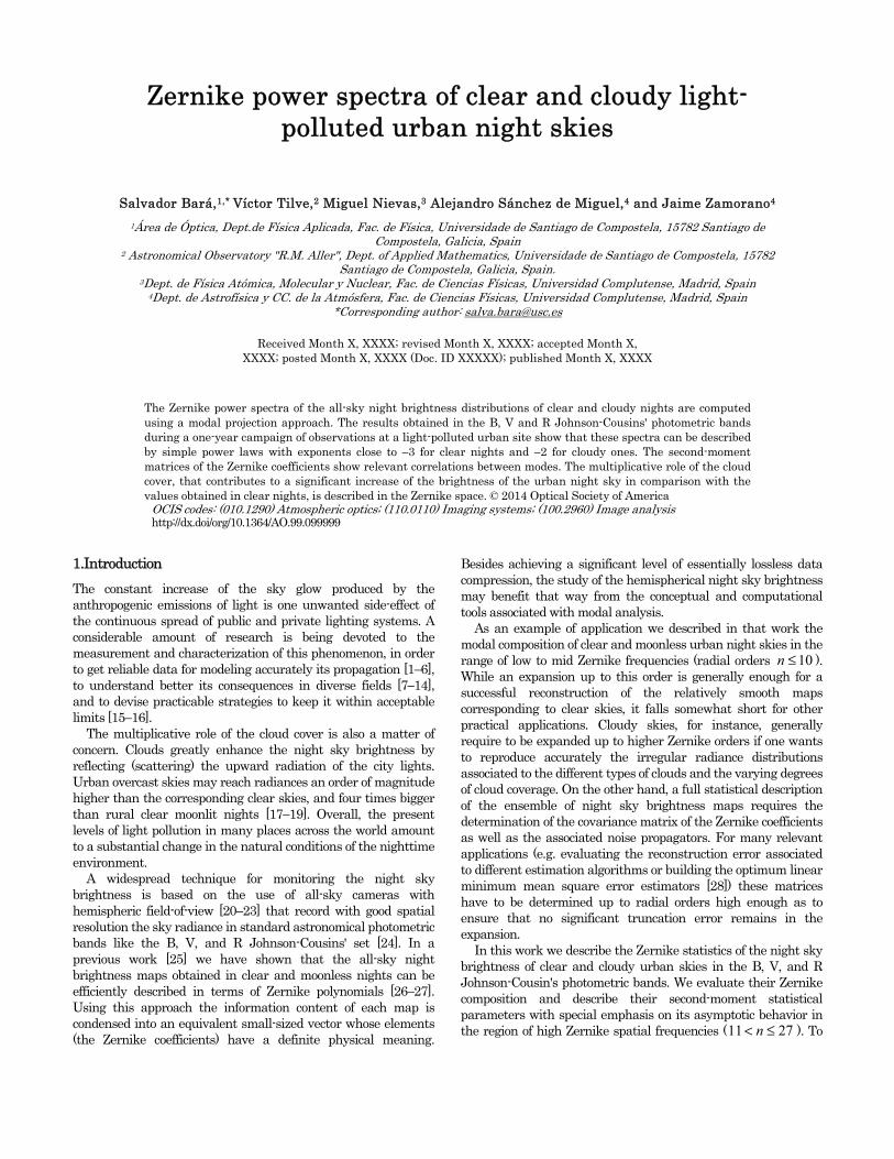
Figure 1 shows an example of reconstruction of a cloudy map in the V band, using 406 Zernike terms (up to radial order n = 27). The estimated Zernike coefficients a were obtained using Eq.(5), with the modal projector P defined in Eq. (4) and a data vector s composed of the brightness values of all pixels contained within the unit radius circle C. Small residual obstacles near the rim of the field-of view were set to zero. The colorbar scale is in units of milliJansky per square arcsecond (mJy/arcsec2).

Figure 1: (Left) All-sky night brightness map taken in the V-band at the UCM observatory the 16th November 2012 at 21:32h (UT). Exposure time: 40 s; (Right) Reconstructed map obtained using 406 Zernike coefficients estimated by modal projection. Uncorrelated zero-mean random gaussian noise with the same variance as that of the noise present in the original image has been added to the reconstructed map.

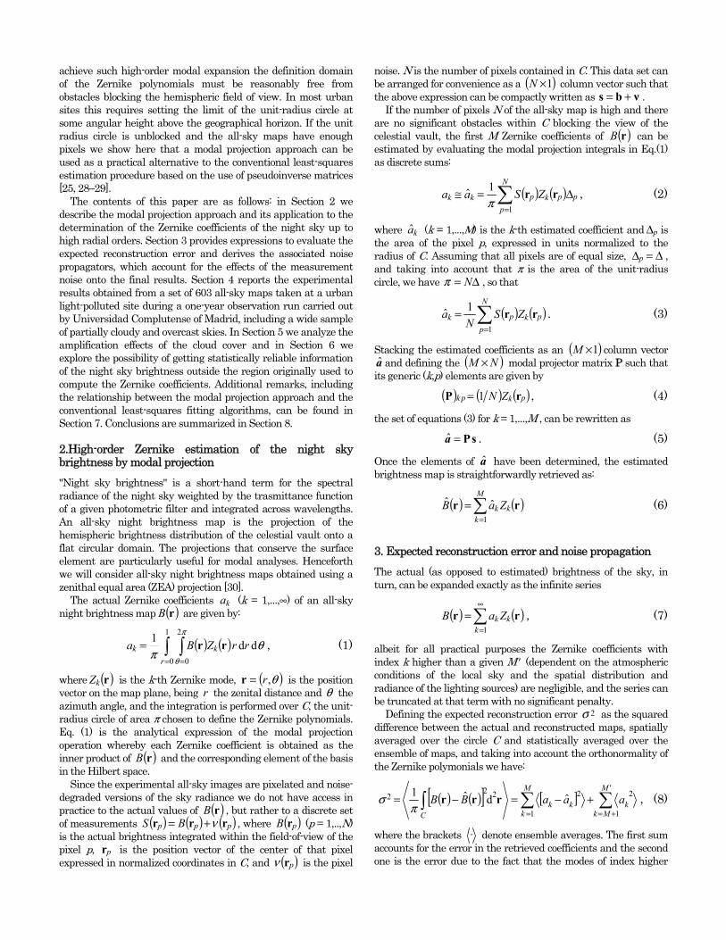
Figure 2. Average values of the first 406 Zernike coefficients (in log10 scale) for clear skies (left column, 80 all-sky maps in each band) and cloudy skies (right column, about 120 maps in each band, see text), in the B, V and R bands (from top to bottom, respectively). Coefficients with average positive values are displayed as blue squares, whereas those with negative values are plotted as red circles. Scale in mJy/arcsec2.

The decimal logarithms of the average values of the Zernike coefficients for each subset of maps (clear/cloudy) at each photometric band are displayed Figure 2. Blue squares correspond to coefficients whose average value is positive, and red circles to those whose average is negative. The first Zernike coefficient 1a , corresponding to the constant term or piston, gives the mean brightness of the sky, spatially averaged over the field of view, in mJy/arcsec2.

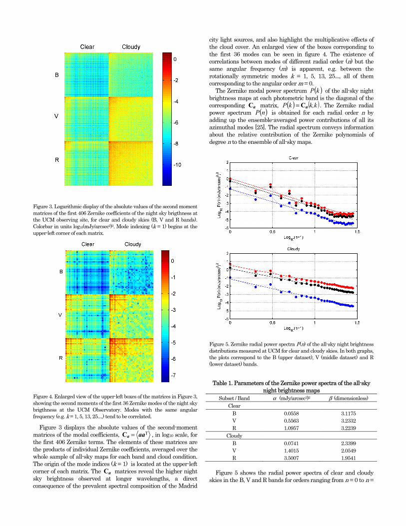
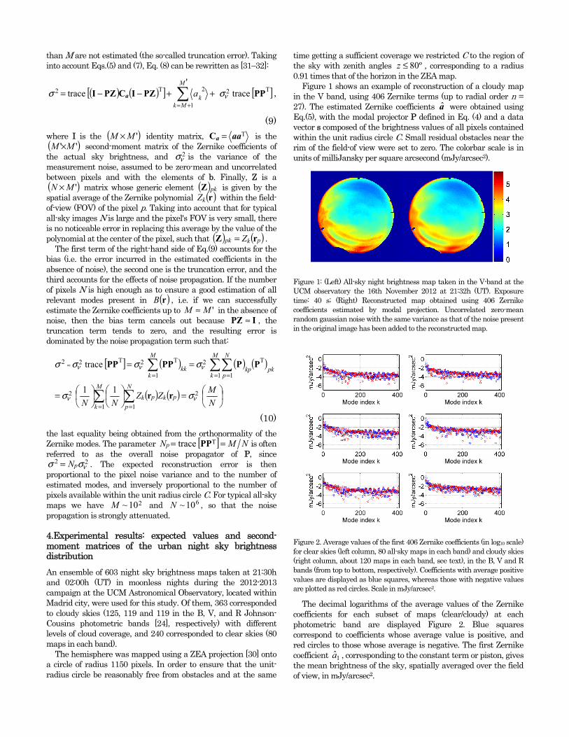
Figure 3. Logarithmic display of the absolute values of the second moment matrices of the first 406 Zernike coefficients of the night sky brigthness at the UCM observing site, for clear and cloudy skies (B, V and R bands). Colorbar in units log10(mJy/arcsec2)2. Mode indexing (k = 1) begins at the upper-left corner of each matrix.

Figure 4. Enlarged view of the upper-left boxes of the matrices in Figure 3, showing the second moments of the first 36 Zernike modes of the night sky brigthness at the UCM Observatory. Modes with the same angular frequency (e.g. k = 1, 5, 13, 25...,) tend to be correlated.

Figure 3 displays the absolute values of the second-moment matrices of the modal coefficients, Taaa =C , in log10 scale, for the first 406 Zernike terms. The elements of these matrices are the products of individual Zernike coefficients, averaged over the whole sample of all-sky maps for each band and cloud condition. The origin of the mode indices (k = 1) is located at the upper-left corner of each matrix. The aC matrices reveal the higher night sky brightness observed at longer wavelengths, a direct consequence of the prevalent spectral composition of the Madrid

city light sources, and also highlight the multiplicative effects of the cloud cover. An enlarged view of the boxes correponding to the first 36 modes can be seen in figure 4. The existence of correlations between modes of different radial order (n) but the same angular frequency (m) is apparent, e.g. between the rotationally symmetric modes k = 1, 5, 13, 25..., all of them corresponding to the angular order m = 0.

The Zernike modal power spectrum ( )kP of the all-sky night brightness maps at each photometric band is the diagonal of the corresponding aC matrix, ( ) ( )k,kkP aC= . The Zernike radial power spectrum ( )nP is obtained for each radial order n by adding up the ensemble-averaged power contributions of all its azimuthal modes [25]. The radial spectrum conveys information about the relative contribution of the Zernike polynomials of degree n to the ensemble of all-sky maps.

Figure 5. Zernike radial power spectra P(n) of the all-sky night brightness distributions measured at UCM for clear and cloudy skies. In both graphs, the plots correspond to the B (upper dataset), V (middle dataset) and R (lower dataset) bands.

Table 1. Parameters of the Zernike power spectra of the all-sky night brightness maps

Subset / Band α (mJy/arcsec2)2 β (dimensionless) Clear

B 0.0558 3.1175 V 0.5563 3.2332 R 1.0957 3.2239

Cloudy B 0.0741 2.3399 V 1.4015 2.0549 R 3.5007 1.9541

Figure 5 shows the radial power spectra of clear and cloudy

skies in the B, V and R bands for orders ranging from n = 0 to n =

27 (Zernike mode indices k = 1 to k = 406). The log-log plots of the spectra show a linear dependence on n of slope −β whose decreasing trends can be approximately described by power laws of the type ( ) ( ) βα −+= 1nnP , with exponents β between 1.9 and 3.2 (Table 1).

The smaller exponents of the power spectra of cloudy skies reflect the fact that these skies need to be expanded up to relatively high Zernike orders (406 terms, nmax = 27) to account for the irregular brightness distributions produced by the different kinds of clouds and the varying degrees of cloud coverage. The comparatively smooth brightness distributions of clear skies, in turn, can be succesfully described using a significantly smaller number of Zernike polynomials (~ 66 terms, nmax = 10) [25].

The parameter α is the value at the origin of the regression line of the log-log ( )nP data set. Since the radial order n = 0 is composed only by the first Zernike term, we have ( ) 2

10 aP ≡ . In consequence, the square root of ( )0P gives us the root mean-square value (averaged over the ensemble of nights) of the mean sky brightness (averaged over directions in the sky). An inspection to the values of in Table 1 reveals at a first glance the increased sky brightness of typical urban overcast nights in comparison with clear ones. The multiplicative role of the cloud cover is analyzed in the next section.

5. Cloud multiplication factor in the Zernike space

The presence of clouds greatly enhances the night sky brightness at urban and suburban sites, in comparison with that of clear skies at the same locations [17−19]. The increased brightness due to the cloud cover depends on several factors related to the composition of the atmosphere and the spectral radiance and geographical distribution of artificial lights [2]. This enhancement by clouds at cities contrasts with what happens at rural locations with pristine dark skies, where clouds rather act as screens that block the propagation of the starlight and the airglow of the upper atmosphere, thus reducing the recorded sky brightness.

Figure 6. Average histogram of the absolute frequencies of the pixel brightness values in the B, V and R bands, for clear (solid line) and cloudy (solid line with dots) skies.

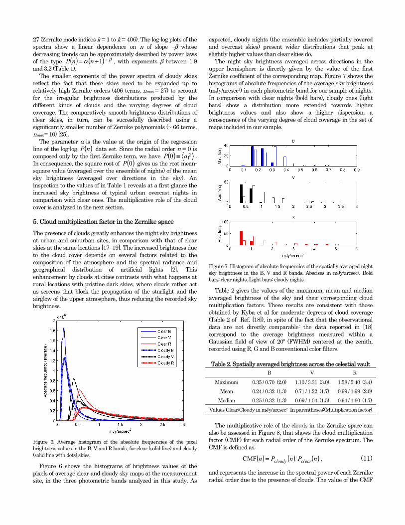
Figure 6 shows the histograms of brightness values of the pixels of average clear and cloudy sky maps at the measurement site, in the three photometric bands analyzed in this study. As

expected, cloudy nights (the ensemble includes partially covered and overcast skies) present wider distributions that peak at slightly higher values than clear skies do.

The night sky brightness averaged across directions in the upper hemisphere is directly given by the value of the first Zernike coefficient of the corresponding map. Figure 7 shows the histograms of absolute frequencies of the average sky brightness (mJy/arcsec2) in each photometric band for our sample of nights. In comparison with clear nights (bold bars), cloudy ones (light bars) show a distribution more extended towards higher brightness values and also show a higher dispersion, a consequence of the varying degree of cloud coverage in the set of maps included in our sample.

Figure 7: Histogram of absolute frequencies of the spatially averaged night sky brightness in the B, V and R bands. Abscises in mJy/arcsec2. Bold bars: clear nights. Light bars: cloudy nights.

Table 2 gives the values of the maximum, mean and median averaged brightness of the sky and their corresponding cloud multiplication factors. These results are consistent with those obtained by Kyba et al for moderate degrees of cloud coverage (Table 2 of Ref. [18]), in spite of the fact that the observational data are not directly comparable: the data reported in [18] correspond to the average brightness measured within a Gaussian field of view of 20º (FWHM) centered at the zenith, recorded using R, G and B conventional color filters.

Table 2. Spatially averaged brightness across the celestial vault B V R

Maximum 0.35 / 0.70 (2.0) 1.10 / 3.31 (3.0) 1.58 / 5.40 (3.4)

Mean 0.24 / 0.32 (1.3) 0.71 / 1.22 (1.7) 0.99 / 1.99 (2.0)

Median 0.25 / 0.32 (1.3) 0.69 / 1.04 (1.5) 0.94 / 1.60 (1.7)

Values Clear/Cloudy in mJy/arcsec2 In parentheses:(Multiplication factor)

The multiplicative role of the clouds in the Zernike space can

also be assessed in Figure 8, that shows the cloud multiplication factor (CMF) for each radial order of the Zernike spectrum. The CMF is defined as:

( ) ( ) ( )nPnPn earclcloudy=CMF , (11)

and represents the increase in the spectral power of each Zernike radial order due to the presence of clouds. The value of the CMF

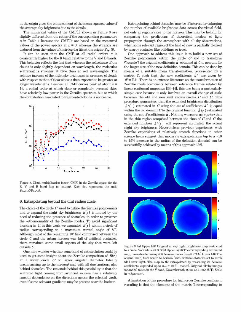
at the origin gives the enhancement of the mean squared value of the average sky brightness due to the clouds.

The numerical values of the CMF(0) shown in Figure 8 are slightly different from the ratios of the corresponding parameters α in Table 1 because the CMF(0) are based on the measured values of the power spectra at n = 0, whereas the α ratios are deduced from the values of their log-log fits at the origin (Fig. 5).

It can be seen that the CMF at all radial orders n is consistently higher for the R band, relative to the V and B bands. This behavior reflects the fact that whereas the reflectance of the clouds is only slightly dependent on wavelength, the molecular scattering is stronger at blue than at red wavelenghts. The relative increase of the night sky brightness in presence of clouds with respect to that of clear skies is then expected to be greater at longer wavelengths. Besides, all CMF curves peak at about n = 16, a radial order at which clear or completely overcast skies have relatively low power in the Zernike spectrum but at which the contribution associated to fragmented clouds is noticeable.

Figure 8. Cloud multiplication factor (CMF) in the Zernike space, for the R, V and B band (top to bottom). Each dot represents the ratio Pcloudy(n)/Pclear(n).

6. Extrapolating beyond the unit radius circle

The choice of the circle C used to define the Zernike polynomials and to expand the night sky brightness ( )rB is limited by the need of reducing the presence of obstacles, in order to preserve the orthonormality of the Zernike modes. To avoid significant blocking in C, in this work we expanded ( )rB within a circle of radius corresponding to a maximum zenital angle of 80º. Although most of the remaining 10º field comprised between the circle C and the urban horizon was full of artificial obstacles, there remained some small regions of the sky that were left outside C.

One may wonder whether some kind of extrapolation could be used to get some insight about the Zernike composition of ( )rB at a wider circle C' of larger angular diameter (ideally encompassing up to the horizon) and, with all due cautions, also behind obstacles. The rationale behind this possibility is that the scattered light coming from artificial sources has a relatively smooth dependence on the directions across the celestial vault, even if some relevant gradients may be present near the horizon.

Extrapolating behind obstacles may be of interest for enlarging the number of available brightness data across the visual field, not only at regions close to the horizon. This may be helpful for comparing the predictions of theoretical models of light propagation through the atmosphere with all-sky observations, when some relevant region of the field of view is partially blocked by nearby obstacles like buildings or trees.

One approach to address this issue is to build a new set of Zernike polynomials within the circle C' and to transform ("rescale") the original coefficients a obtained at C to account for the larger size of the new definition domain. This can be done by means of a suitable linear transformation, represented by a matrix T, such that the new coefficients 'a are given by

a'a ˆˆ T= . There is an extense literature on the transformation of Zernike mode coefficients between reference frames related by linear conformal mappings [33−44], this one being a particularly simple case because it only involves an overall change of scale between the old and new unit radius circles C and C'. This procedure guarantees that the extended brightness distribution

( )r'B estimated in C' using the set of coefficients 'a is equal within the old domain C to the original function ( )rB estimated using the set of coefficients a . Nothing warrants us a priori that in the thin region comprised between the rims of C and C' the extended function ( )r'B will represent accurately the actual night sky brightness. Nevertheless, previous experiences with Zernike expansions of relatively smooth functions in other science fields suggest that moderate extrapolations (up to a ~10 to 15% increase in the radius of the definition domain) can be successfully achieved by means of this approach [32].

Figure 9: (a) Upper left: Original all-sky night brightness map, restricted to a circle C of radius z = 80º; (b) Upper right: The corresponding estimated map, reconstructed using 406 Zernike modes (nmax = 27); (c) Lower left: The original map, from zenith to horizon (with artificial obstacles set to zero); (d) Lower right: The map in (b) extrapolated by reescaling its Zernike coefficients, expanded up to nmax = 12 (91 modes). Original all-sky images (a) and (c) taken in the V band, November 6th, 2012, at 21:25h (UT). Scale in mJy/arcsec2.

A limitation of this procedure for high order Zernike coefficient rescaling is that the elements of the matrix T corresponding to

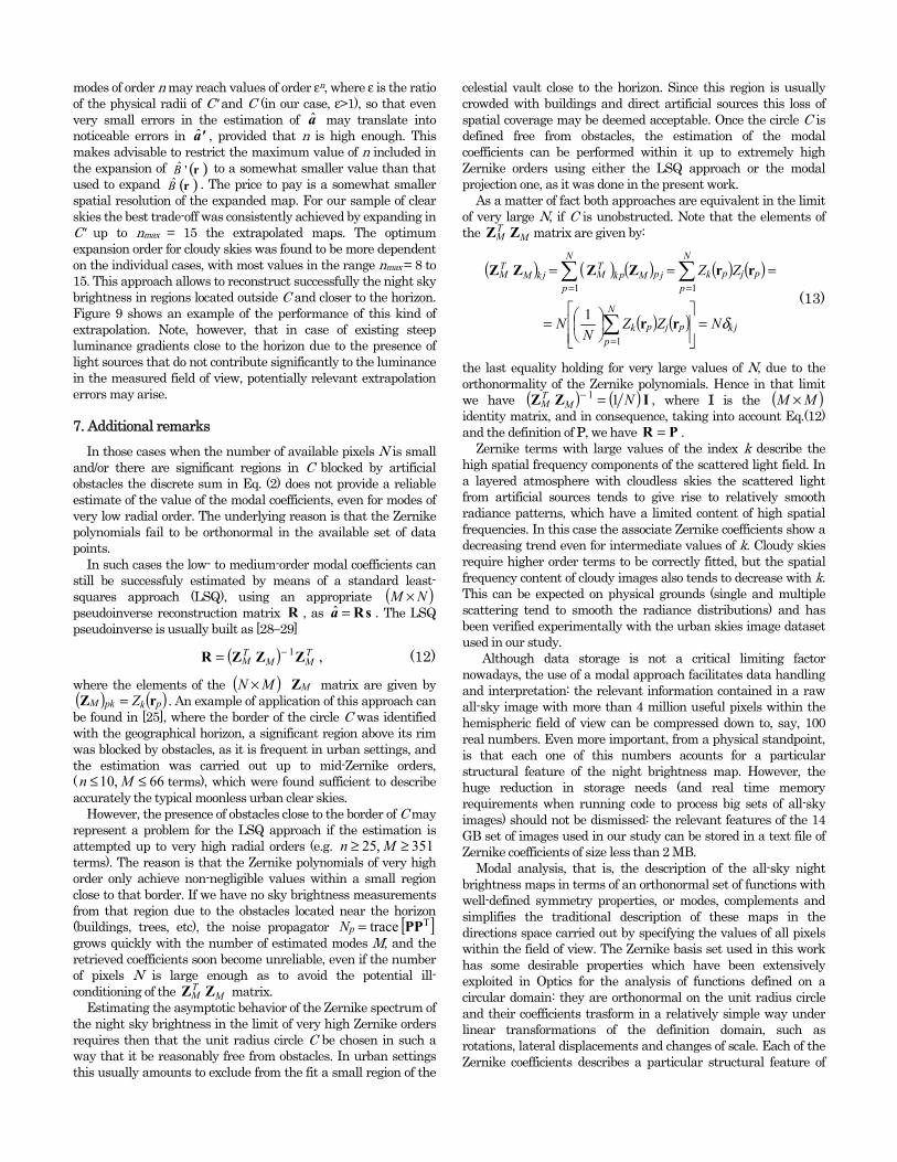
modes of order n may reach values of order εn, where ε is the ratio of the physical radii of C' and C (in our case, ε>1), so that even very small errors in the estimation of a may translate into noticeable errors in 'a , provided that n is high enough. This makes advisable to restrict the maximum value of n included in the expansion of ( )r'B to a somewhat smaller value than that used to expand ( )rB . The price to pay is a somewhat smaller spatial resolution of the expanded map. For our sample of clear skies the best trade-off was consistently achieved by expanding in C' up to nmax = 15 the extrapolated maps. The optimum expansion order for cloudy skies was found to be more dependent on the individual cases, with most values in the range nmax = 8 to 15. This approach allows to reconstruct successfully the night sky brightness in regions located outside C and closer to the horizon. Figure 9 shows an example of the performance of this kind of extrapolation. Note, however, that in case of existing steep luminance gradients close to the horizon due to the presence of light sources that do not contribute significantly to the luminance in the measured field of view, potentially relevant extrapolation errors may arise. 7. Additional remarks

In those cases when the number of available pixels N is small and/or there are significant regions in C blocked by artificial obstacles the discrete sum in Eq. (2) does not provide a reliable estimate of the value of the modal coefficients, even for modes of very low radial order. The underlying reason is that the Zernike polynomials fail to be orthonormal in the available set of data points.

In such cases the low- to medium-order modal coefficients can still be successfuly estimated by means of a standard least-squares approach (LSQ), using an appropriate ( )NM × pseudoinverse reconstruction matrix R , as sR=a . The LSQ pseudoinverse is usually built as [28−29]

( ) TMM

TM ZZZR 1−= , (12)

where the elements of the ( )MN × MZ matrix are given by ( ) ( )pkpkM Z rZ = . An example of application of this approach can be found in [25], where the border of the circle C was identified with the geographical horizon, a significant region above its rim was blocked by obstacles, as it is frequent in urban settings, and the estimation was carried out up to mid-Zernike orders, ( 66 ,10 ≤≤ Mn terms), which were found sufficient to describe accurately the typical moonless urban clear skies.

However, the presence of obstacles close to the border of C may represent a problem for the LSQ approach if the estimation is attempted up to very high radial orders (e.g. 351 ,25 ≥≥ Mn terms). The reason is that the Zernike polynomials of very high order only achieve non-negligible values within a small region close to that border. If we have no sky brightness measurements from that region due to the obstacles located near the horizon (buildings, trees, etc), the noise propagator [ ]Ttrace PP=pN grows quickly with the number of estimated modes M, and the retrieved coefficients soon become unreliable, even if the number of pixels N is large enough as to avoid the potential ill-conditioning of the M

TM ZZ matrix.

Estimating the asymptotic behavior of the Zernike spectrum of the night sky brightness in the limit of very high Zernike orders requires then that the unit radius circle C be chosen in such a way that it be reasonably free from obstacles. In urban settings this usually amounts to exclude from the fit a small region of the

celestial vault close to the horizon. Since this region is usually crowded with buildings and direct artificial sources this loss of spatial coverage may be deemed acceptable. Once the circle C is defined free from obstacles, the estimation of the modal coefficients can be performed within it up to extremely high Zernike orders using either the LSQ approach or the modal projection one, as it was done in the present work.

As a matter of fact both approaches are equivalent in the limit of very large N, if C is unobstructed. Note that the elements of the M

TM ZZ matrix are given by:

( ) ( ) ( ) ( ) ( )

( ) ( ) jk

N

p

pjpk

N

p

pjpkjpM

N

ppk

TMjkM

TM

NZZN

N

ZZ

δ=

=

===

=

==

1

11

1rr

rrZZZZ

(13)

the last equality holding for very large values of N, due to the orthonormality of the Zernike polynomials. Hence in that limit we have ( ) ( ) IZZ NM

TM 11 =− , where I is the ( )MM ×

identity matrix, and in consequence, taking into account Eq.(12) and the definition of P, we have PR = .

Zernike terms with large values of the index k describe the high spatial frequency components of the scattered light field. In a layered atmosphere with cloudless skies the scattered light from artificial sources tends to give rise to relatively smooth radiance patterns, which have a limited content of high spatial frequencies. In this case the associate Zernike coefficients show a decreasing trend even for intermediate values of k. Cloudy skies require higher order terms to be correctly fitted, but the spatial frequency content of cloudy images also tends to decrease with k. This can be expected on physical grounds (single and multiple scattering tend to smooth the radiance distributions) and has been verified experimentally with the urban skies image dataset used in our study.

Although data storage is not a critical limiting factor nowadays, the use of a modal approach facilitates data handling and interpretation: the relevant information contained in a raw all-sky image with more than 4 million useful pixels within the hemispheric field of view can be compressed down to, say, 100 real numbers. Even more important, from a physical standpoint, is that each one of this numbers acounts for a particular structural feature of the night brightness map. However, the huge reduction in storage needs (and real time memory requirements when running code to process big sets of all-sky images) should not be dismissed: the relevant features of the 14 GB set of images used in our study can be stored in a text file of Zernike coefficients of size less than 2 MB.

Modal analysis, that is, the description of the all-sky night brightness maps in terms of an orthonormal set of functions with well-defined symmetry properties, or modes, complements and simplifies the traditional description of these maps in the directions space carried out by specifying the values of all pixels within the field of view. The Zernike basis set used in this work has some desirable properties which have been extensively exploited in Optics for the analysis of functions defined on a circular domain: they are orthonormal on the unit radius circle and their coefficients trasform in a relatively simple way under linear transformations of the definition domain, such as rotations, lateral displacements and changes of scale. Each of the Zernike coefficients describes a particular structural feature of

the all-sky map, as revealed by the geometry of the corresponding Zernike mode. Of course, other basis sets can also be used for this purpose. Fourier transforms, for instance, are standard tools for analyzing the spatial frequency content of images and can also be successfully applied to the study of all-sky night brightness maps. However, the Fourier spectra of these maps is not band-limited, due to the fact that their spatial definition domain is bounded by the horizon line. Since the two-dimensional funtion describing the sky brightness has a sharp discontinuity at that border, the Fourier spectrum of an all-sky night brightness map spreads up to infinitely high spatial frequencies. The Zernike basis avoids this issue because its definition domain is coincident with that of the maps.

In this work we provide a complete account of the second-order statistics of the night sky brightness in the Zernike space. The key results are the explicit values of the second-moment matrices aC of the Zernike coefficients, described in section 4. These

second-moment matrices contain in their diagonal elements the Zernike power spectrum but their usefulness goes well beyond that: they provide key information about the correlations between the Zernike modes, which is essential for a complete characterization of the night sky brightness statistics. Additionally, the knowledge of the aC matrices -together with the average values of the Zernike coefficients and the noise statistics- is all that is required to assess the performance of different strategies for recovering the all-sky night brightness maps from discrete sets of measurements made with instruments of arbitrary spatial resolution using linear estimation algorithms, of which all-sky cameras are just an example. These evaluations may be carried out by any interested reader by applying Eq.(9) to their particular instruments (through the proper definition of matrix Z) and intended reconstruction algorithms (through the appropriate choice of the matrix P). The aC data obtained in the present study are freely available upon request.

8. Conclusions

In this work we have shown that the Zernike coefficients of all-sky night brightness maps, under clear and cloudy conditions, can be efficiently computed by direct modal projection with the proviso that the unit radius circle C where this calculation is performed be reasonably free from obstacles. If the number of available pixels is enough high, the modal projection approach enables to extend the computation of the Zernike power spectrum up to very high radial orders n, allowing thus to assess its asymptotic behavior in the region of high spatial frequencies.

After analyzing the field of view of our hemispherical images and in order to fulfill the condition that the unit-radius circle be reasonably free from obstacles we have chosen its radius such that it corresponds to a zenithal angle z = 80º. We have shown that with some due cautions it is possible to perform a moderate extrapolation of the results obtained therein to unit-radius circles of larger angular size, including its extension up to the horizon, by a simple linear transformation of the Zernike coefficients. Since the elements of the transformation matrix used to compute the extrapolated Zernike coefficients diverge exponentially with n, tending to increase without bound the effects of noise, the extrapolation must be judiciously restricted to the mid-frequency range (nmax about 8 to 15). In such way the values of the night sky brightness in a small region outside C can be satisfactorily

estimated, at the price of a somewhat smaller spatial resolution of the reconstructed maps due to the limitation of the Zernike modes included in the expansion.

We have applied this approach to compute the relevant statistical parameters of the night skies at the UCM observatory, an urban site located within Madrid city with high levels of light pollution. The results show the greater night sky brightness present at the R band, in comparison with that of the V and B bands, in that order. This is a direct consequence of the prevalent spectral composition of the Madrid city lights. We have found that the Zernike power spectra of clear and cloudy nights at each band can be described by simple power laws. Whereas for clear skies the exponents of these laws are close to −3, cloudy skies are better described by exponents close to −2, reflecting the fact that more terms of the Zernike basis are required to represent adequately the more irregular sky brightness distribution produced by the reflections of the lights at the base of the clouds. Relevant correlations between Zernike modes have been found under both atmospheric conditions, as revealed by the second moment matrices of the Zernike coefficients.

It shall be stressed that the Zernike expansion, as such, does not allow to forecast directly the sky luminance in regions distant from the one where the all-sky images were acquired. The Zernike coefficients depend on the measurement location: they shall be expected to change with the observer's position within a city, in order to account for the changes in the corresponding all-sky night brightness distributions.

Our results highlight the multiplicative role of the cloud cover, more pronounced at the R band in comparison with what happens at shorter wavelenghts, that are more efficiently scattered than the longer ones in a clear atmosphere. These results, obtained in the Zernike space, are consistent with previous findings reported in the spatial domain. Particularly high multiplication factors were found for all photometric bands at intermediate Zernike frequencies ( )16≈n , an effect probably related to the size distribution of the clouds present in the sample.

Acknowledgments

This work was partially funded by the Xunta de Galicia, Programa de Consolidación e Estruturación de Unidades de Investigación Competitivas, grant CN 2012/156, the Spanish Ministry of Science and Innovation MICINN (AYA2012-30717, AYA2012-31277, AYA2013-46724-P, and FPA2010-22056-C06-06), the Spanish program of International Campus of Excellence Moncloa (CEI) and the Madrid Regional Government through the SpaceTec Project (S2013/ICE-2822). A. Sánchez de Miguel was supported by an FPU grant from MICINN. This work was developed within the framework of the Spanish Network for Light Pollution Studies (Ministerio de Economía y Competitividad, Acción Complementaria AYA2011-15808-E). Useful comments from two anonymous reviewers are also acknowledged.

References

1. R. H. Garstang, “Model for artificial night-sky

illumination,” Publ. Astron. Soc. Pac. 98, 364–375 (1986).

2. M. Kocifaj, “Light-pollution model for cloudy and cloudless night skies with ground-based light sources,” Appl. Opt. 46, 3013-3022 (2007).

3. M. Kocifaj, “Light pollution simulations for planar ground-based light sources,” Appl. Opt. 47, 792-798 (2008).

4. M. Kocifaj, “A numerical experiment on light pollution from distant sources” Mon. Not. R. Astron. Soc. 415, 3609–3615 (2011).

5. P. Cinzano and F. Falchi, “The propagation of light pollution in the atmosphere,” Mon. Not. R. Astron. Soc. 427, 3337–3357 (2012).

6. M. Aubé and M. Kocifaj, “Using two light-pollution models to investigate artificial sky radiances at Canary Islands observatories,” Mon. Not. R. Astron. Soc. 422, 819–830 (2012).

7. M. F. Walker, “The California Site Survey,” Publ. Astron. Soc. Pac. 82, 672-698 (1970).

8. P. Cinzano, F. Falchi and C. Elvidge, “The first world atlas of the artificial night sky brightness,” Mon. Not. R. Astron. Soc. 328, 689–707 (2001).

9. K. Thapan, J. Arendt, and D.J. Skene, “An action spectrum for melatonin suppression: evidence for a novel non-rod, non-cone photoreceptor system in humans,” J. Physiol. 535, 261–267 (2001).

10. D. M. Berson, F. A. Dunn and M. Takao, “Phototransduction by Retinal Ganglion Cells That Set the Circadian Clock,” Science 295, 1070-1073 (2002).

11. F. Hölker, C. Wolter, E. K. Perkin, and K. Tockner, “Light pollution as a biodiversity threat,” Trends Ecol. Evol. 25, 681-682 (2010).

12. C. S. J. Pun and C. W. So, "Night-sky brightness monitoring in Hong Kong. A city-wide light pollution assessment," Environ. Monit. Assess. 184, 2537–2557 (2012).

13. K. J. Gaston, J. Bennie, T. W. Davies, and J. Hopkins, "The ecological impacts of nighttime light pollution: a mechanistic appraisal," Biological Reviews 88, 912–927 (2013).

14. K. J. Gaston, J. P. Duffy, S. Gaston, J. Bennie, and T. W. Davies, "Human alteration of natural light cycles: causes and ecological consequences," Oecologia 176, 917–931 (2014).

15. C. Marín and J. Jafari (Eds.), Starlight, A Common Heritage, Starlight Initiative-Instituto de Astrofísica de Canarias (IAC, 2007).

16. C. C. M. Kyba, A. Hänel, and F. Hölker, "Redefining efficiency for outdoor lighting," Energy Environ. Sci. 7, 1806-1809 (2014).

17. C. C. M. Kyba, T. Ruhtz, J. Fischer, F. Hölker, "Cloud Coverage Acts as an Amplifier for Ecological Light Pollution in Urban Ecosystems," PLoS ONE 6(3):e17307 (2011) .

18. C. C. M. Kyba, T. Ruhtz, J. Fischer, and F. Hölker, "Red is the new black: how the colour of urban skyglow varies with cloud cover," Mon. Not. R. Astron. Soc. 425, 701–708 (2012).

19. C. C. M. Kyba, K. Pong Tong, et al., "Worldwide variations in artificial skyglow," Scientific Reports 5, 8409 (2015) doi:10.1038/srep08409

20. K. Tohsing, M. Schrempf, S. Riechelmann, H. Schilke, and G. Seckmeyer, “Measuring high-resolution sky luminance distributions with a CCD camera,” Appl. Opt. 52, 1564-1573 (2013).

21. D.M. Duriscoe, C.B. Luginbuhl, and C.A. Moore, “Measuring Night-Sky Brightness with a Wide-Field CCD Camera,” Publ. Astron. Soc. Pac. 119, 192–213 (2007).

22. O. Rabaza, D. Galadí-Enríquez, A. Espín-Estrella, and F. Aznar-Dols, “All-Sky brightness monitoring of light

pollution with astronomical methods,” J. Environ. Manage. 91, 1278-1287 (2010).

23. J. Aceituno, S.F. Sánchez, F.J. Aceituno, D. Galadí-Enríquez, J.J. Negro, R.C. Soriguer, and G. Sanchez-Gomez, “An All-Sky Transmission Monitor: ASTMON,” Publ. Astron. Soc. Pac. 123, 1076–1086 (2011).

24. M. S. Bessell, "UBVRI photometry II: The Cousins VRI system, its temperature and absolute flux calibration, and relevance for two-dimensional photometry," Publ. Astron. Soc. Pac. 91, 589–607 (1979).

25. S. Bará, M. Nievas, A. Sánchez de Miguel, and J. Zamorano, "Zernike analysis of all-sky night brightness maps," Appl. Opt. 53, 2677-2686 (2014).

26. F. Zernike, "Beugungstheorie des Schneidenverfahrens und seiner verbesserten Form, der Phasenkontrastmethode," Physica 1, 689-704 (1934).

27. M. Born and E. Wolf, Principles of Optics (Cambridge University Press, 1998), pp. 464-466, 767-772.

28. P. B. Liebelt, An Introduction to Optimal Estimation (Addison-Wesley, Reading, MA, 1967).

29. J. Herrmann, “Least-squares wave front errors of minimum norm,” J. Opt. Soc. Am. 70, 28-35 (1980).

30. M. R. Calabretta and E. W. Greisen, "Representation of celestial coordinates in FITS," Astronomy and Astrophysics 395, 1077-1122 (2002).

31. S. Bará, E. Pailos and J. Arines, Signal-to-noise ratio and aberration statistics in ocular aberrometry, Optics Lett. 37, 2427-2429 (2012).

32. S. Bará, E. Pailos, J. Arines, N. López-Gil, and L. Thibos, Estimating the eye aberration coefficients in resized pupils: Is it better to refit or to rescale?, J. Opt. Soc. Am. A 31, 114-123 (2014).

33. J. Schwiegerling, "Scaling Zernike expansion coefficients to different pupil sizes," J. Opt. Soc. Am. A 19, 1937-1945. (2002).

34. C.E. Campbell, "Matrix method to find a new set of Zernike coefficients from an original set when the aperture radius is changed," J. Opt. Soc. Am. A 20, 209-217 (2003).

35. G.M. Dai, "Scaling Zernike expansion coefficients to smaller pupil sizes: a simpler formula," J. Opt. Soc. Am. A 23, 539-543 (2006).

36. H. Shu, L. Luo, G. Han, and J.L. Coatrieux, "General method to derive the relationship between two sets of Zernike coefficients corresponding to different aperture sizes," J. Opt. Soc. Am. A 23, 1960-1968 (2006).

37. S. Bará, J. Arines, J. Ares, and P. Prado, "Direct transformation of Zernike eye aberration coefficients between scaled, rotated and/or displaced pupils," J. Opt. Soc. Am. A 23, 2061-2066 (2006).

38. A.J. Janssen and P Dirksen, "Concise formula for the Zernike coefficients of scaled pupils," Journal of Microlithography, Microfabrication, and Microsystem. 5, 030501-1–030501-3 (2006).

39. L. Lundström and P. Unsbo, "Transformation of Zernike coefficients: scaled, translated, and rotated wavefronts with circular and elliptical pupils," J. Opt. Soc. Am. A 24, 569-577 (2007).

40. A.J. Janssen, S. van Haver, P. Dirksen and J.J. Braat, "Zernike representation and Strehl ratio of optical systems with variable numerical aperture," J. Mod. Opt. 55, 1127-1157 (2008).

41. J.A. Díaz, J. Fernández-Dorado, C. Pizarro and J. Arasa, "Zernike coefficients for concentric, circular scaled pupils: an equivalent expansion," J. Mod. Opt. 56, 149-155 (2009).

42. K. Dillon, "Bilinear wavefront transformation," J. Opt. Soc. Am. A 26, 1839-1846 (2009).

43. V.N. Mahajan, "Zernike coefficients of a scaled pupil," Appl. Opt. 49, 5374-5377 (2010).

44. E. Tatulli, "Transformation of Zernike coefficients: a Fourier-based method for scaled, translated, and rotated wavefront apertures," J. Opt. Soc. Am. A 30, 726-732 (2013).