


Idiomas
Páginas
Jurídico


FACULTAT DE MEDICINA – DEPARTAMENT DE SALUT PÚBLICA
TESI DOCTORAL
CONCORDANÇA:
NOUS PROCEDIMENTS I APLICACIONS
U U U
B B B
UNIVERSITAT DE BARCELONA

Josep Lluís Carrasco Jordan
TESI DOCTORAL
UNIVERSITAT DE BARCELONA
FACULTAT DE MEDICINA – DEPARTAMENT DE SALUT PÚBLICA
Programa de doctorat: Biometria i estadística. Bienni 1999-2001
CONCORDANÇA:

NOUS PROCEDIMENTS I APLICACIONS
Memòria presentada per en Josep Lluís Carrasco i Jordan
per optar al títol de doctor per la Universitat de Barcelona
sota la direcció del doctor Lluís Jover.
VIST I PLAU
El director de la tesi
Dr. Lluís Jover Armengol
Professor Titular de la Facultat de la Medicina. Universitat de Barcelona.

Índex
Agraïments _____________________________________________________________XI
Capítol 1. Introducció ______________________________________________________1
Métodos estadísticos para evaluar la concordancia entre medidas. Josep Lluís
Carrasco i Lluís Jover (en premsa a Medicina Clínica)____________________9
Capítol 2. El Coeficient de Concordança
Introducció_____________________________________________________25
Estimating the Generalized Concordance Correlation Coefficient through
Variance Components. Josep Lluís Carrasco i Lluís Jover (en premsa a
Biometrics) ____________________________________________________26
Estimació del Coeficient de Concordança amb dades de recompte_________47
Apèndix I__________________________________________________64
Apèndix II _________________________________________________71
Capítol 3. El Model d’Equació Estructural aplicat a Bioequivalència
Introducció ____________________________________________________79
Assessing Individual Bioequivalence using the Structural Equation Model. Josep
Lluís Carrasco i Lluís Jover (Statistics in Medicine 22:901-912, 2003)_______
79
The Structural Error-in-Equation Model to evaluate Individual Bioequivalence.
Josep Lluís Carrasco i Lluís Jover (en revisió a Journal of Pharmacokinetics
and Pharmacodynamics)__________________________________________101
Capítol 4. Resum i Conclusions _______________________________________________119
Bibliografia _________________________________________________________125

AGRAÏMENTS
Per explicar la història d’aquesta tesi ens hem d’anar fins la tardor de l’any 1995, quan al Lluís se li
van creuar els cables i em va cridar per col·laborar amb ell en un projecte de quatre mesos. Quantes
vegades t’has penedit, Lluís? El projecte estava relacionat amb l’error de mesura i la concordança
dels analitzadors automàtics i va ser aquí quan vam començar a treballar amb el tema d’aquesta tesi,
clar que aleshores no ho sabíem. Des d’aleshores fins ara tot el que s’ha fet ha estat gràcies a en
Lluís, a la seva visió i forma de treballar que ha intentat transmetre’m (espero que amb èxit). Per
tant el primer i més gran agraïment ha de ser per en Lluís, el meu Mestre i autèntica alma mater
d’aquesta tesi.
També unes paraules d’agraïment per la Rosa Abellana, que m’ha suportat en els darrers cinc anys
que hem compartit despatx, alegries i penes. Gràcies Rosa.
A tothom del departament de Salut Pública i del Departament d’Estadística de la Universitat de
Barcelona que d’una manera o d’altra ha col·laborat per a dur a bon port aquesta tesi, i de manera
especial a la Geòrgia i al Jaume que han viscut el dia a dia de la tesi, i al Dr. Ricard Tresserres que
sempre ha estat disposat a donar un cop de mà.
També vull agrair a l’Albert Cobos les converses instructives que hem mantingut al llarg dels últims
anys i que m’han ajudat a aclarir dubtes i problemes.
A en Quim Barris i la seva companya Maria, que m’ha donat un cop de mà en l’estil de la tesi.
Espero que no trobis gaires incorreccions en aquests agraïments.
A l’Héctor i la Núria de Saragossa perquè les estades amb ells sempre han estat molt estimulants.
També gràcies a l’Àlex i i la Inma amb els que he compartit molts bon moments que m’han ajudat a
carregar pil·les.
A Joan Gaspart, perquè gràcies a la seva gestió el meu interès pel futbol ha anat minvant en els
darrers tres anys deixant-me el temps suficient per poder concloure la tesi.
Gràcies als Bicharracos, equip de futbol-sala de Montbau que ha servit de vàlvula d’escapament.
¡Ánimo Bichos, de derrota en derrota hasta la victória final!. Gràcies també a la Serra de Collserola,

perquè tot anant en mountain-bike pels seus camins se’m van ocórrer algunes de les idees que es
troben a la tesi.
Per haver-me ajudat a superar tots els tràngols que m’he trobat en aquesta aventura, gràcies a: El
Jueves, als Monty Pyton, als programes del Buenafuente, a l’Sport i la seva informació “objectiva”,
a Quino i Mafalda, a Astèrix i Obèlix, a en Tintín i llamp de llamp no m’oblidaré pas d’en Capità
Haddock.
Al Dr. Watson i les seves visites inesperades sempre en el “millor” moment.
Als meus pares i a la meva àvia Rita per l’esforç que han fet tota la vida per a que el dròpol del seu
fill i net fes alguna cosa de profit.
A Buck, l’Alaskan Malamute dels meus pares i el llepador més ràpid que he conegut (sempre que
ell vulgui, és clar).
A Teresa, la meva companya, que mai m’ha deixat que em dormís als llorers i sempre m’ha
recolzat. Ella és la motivació de tot plegat.

CAPÍTOL 1
CAPÍTOL 1. INTRODUCCIÓ
3
INTRODUCCIÓ
Fiabilitat i concordança dels mètodes de mesura
La fiabilitat dels mètodes de mesura és un aspecte fonamental per a garantir la qualitat de tota
activitat basada en la presa de decisions mitjançant les valoracions provinents d’aquests
mètodes. Les Ciències de la Salut són una d’aquestes activitats on contínuament es prenen
decisions derivades dels resultats d’algun tipus de mesura, ja sigui, per exemple, la valoració
subjectiva del professional de la salut a partir d’una placa de tòrax, o el diagnòstic d’un
pacient derivat dels resultats d’una analítica. Aquest fet fa necessari que el professional tingui
una certa seguretat en els mètodes que utilitza per que la pràctica mèdica sigui eficient.
El principal problema que es pot derivar d’un mètode de mesura no fiable és, sens dubte, la
classificació o diagnòstic incorrectes d’un pacient, però el fet de què es mesuri amb error
també provoca que s’observin associacions atenuades entre variables, per exemple entre una
malaltia i un factor de risc, o el fet que la potència dels contrasts d’hipòtesi sigui inferior a la
desitjada o estimada en principi (Fleiss, 1986). Així doncs, per estudiar la fiabilitat d’un
mètode de mesura és necessari mesurar repetides vegades la característica que es desitja
valorar a un set de mostres o individus susceptibles de tenir la característica en qüestió. Sota
aquest disseny, el model de mesura subjacent que genera les dades observades es pot definir
com
ij*iij eXX +β+α=
on Xij correspon a la mesura j-èssima realitzada sobre l’individu i-èssim, *iX representa la
mesura real desconeguda de l’individu i-èssim i eij és la variació aleatòria que es produeix en
realitzar cada mesura i que habitualment s’assumeix centrada a zero. Si ( ) *iij XXE = es
considera que el mètode de mesura no té biaix i per tant se’l qualifica de vàlid. Per tant α i β
es relacionen amb l’exactitud del mètode, on α expressa el biaix sistemàtic constant mentre
que β indica el biaix sistemàtic proporcional. A mode d’exemple podríem imaginar una
balança que sistemàticament mesura 2 kg de més (biaix constant) o que sistemàticament dona
1,5 vegades més que el pes real (biaix proporcional). Naturalment el biaix sistemàtic pot ser
corregit si es disposés informació sobre *iX mitjançant un mètode lliure d’error (gold
standard). L’acte de corregir el biaix sistemàtic és conegut com a calibració de l’instrument
de mesura.
CAPÍTOL 1. INTRODUCCIÓ
4
D’altra banda, l’error aleatori eij es relaciona amb la precisió de l’instrument donat que ens
informa de la variació de les mesures al voltant del valor real *iX . Així un instrument lliure
d’error haurà de ser exacte (sense biaixos) i amb una variabilitat de l’error de mesura igual a
zero. Òbviament aquesta situació és força ideal de manera que per considerar un mètode
fiable serà suficient que es caracteritzi per manca de biaix sistemàtic i que la variabilitat de
l’error es mantingui dintre d’uns límits acceptables.
Una altra qüestió és la intercanviabilitat entre mètodes de mesura, és a dir, la concordança
entre diferents mètodes. Independentment de si els mètodes són fiables o no, és interessant
considerar les implicacions que pot tenir la substitució d’un mètode de mesura per un altre.
Per exemple, es va estudiar les implicacions que tenia el canvi d’un esfigmomanòmetre
manual per un d’automàtic respecte a l’estimació puntual de la prevalença d’hipertensió
(Pardell et al., 2001), arribant-se a la conclusió que amb l’aparell automàtic l’estimació
puntual augmentava un 3% (19% amb l’aparell manual, 22% amb l’aparell automàtic). La
concordança entre instruments de mesura també es pot descompondre en exactitud i precisió,
on l’exactitud vindria representada per la igualtat de mitjanes entre ambdós mètodes, és a dir,
que en mitjana mesurin el mateix. Pel que fa a la precisió, des d’un punt de vista estricte seria
necessari que els instruments no presentessin error de mesura, però aquesta situació és irreal,
sent suficient que els errors de mesura siguin similars i dintre d’uns límits tolerables que facin
que l’error sigui menyspreable.
Tant per mesurar la fiabilitat d’un mètode com la intercanviabilitat entre instruments de
mesura sovint les tècniques estadístiques acostumen a ser les mateixes, diferenciant-se en el
matís de que en el primer cas es vol mesurar com concorda un instrument amb ell mateix
mentre que en el segon cas es vol avaluar com concorden diferents mètodes de mesura.
Aquestes tècniques es poden classificar, a gran trets, com a “agregades” o “desagregades”, tot
depenent de com es du a terme l’avaluació de la concordança. Així, un procediment agregat
valora la concordança globalment mitjançant un índex o coeficient, en canvi un procediment
desagregat es caracteritza per estudiar la concordança valorant per separat cadascun dels
errors que es poden produir en mesurar.
Els procediments per a avaluar la concordança també varien en funció de la naturalesa de les
dades i de l’escala de mesura, de forma que existeixen procediments diferents segons es tracti
de dades qualitatives o quantitatives.
CAPÍTOL 1. INTRODUCCIÓ
5
Concordança amb dades qualitatives
El coeficient més popular per a mesurar la concordança entre mètodes de mesura en una
escala qualitativa és el coeficient kappa (Cohen, 1960). Per descriure aquest coeficient
suposem que dos instruments, A i B, mesuren a una sèrie d’individus una característica
qualitativa en escala nominal, per exemple, “Normal” i “Patològic”. Definim π ij com la
probabilitat de que quan l’avaluador A mesura i, l’avaluador B mesuri j. El coeficient kappa
es defineix com
∑∑∑
++
++
ππ−
ππ−π=κ
ii
iiii
1
on π i+ i π+i representen les probabilitats marginals de cada avaluador. Aquest índex compara
la probabilitat total de concordança respecte l’esperada per atzar, i es reescala de forma que
un valor d’1 implica concordança perfecta mentre que un valor de 0 significa que els
avaluadors mesuren de forma independent. Aquest índex representa una mesura agregada
donat que valora la concordança entre avaluadors mitjançant un únic valor.
S’han realitzat altres versions del coeficient kappa (Bloch and Kraemer, 1989), però una
menció especial es mereix la versió per a variables ordinals. Quan la característica es
mesurada en una escala ordinal la discordança entre les categories no té la mateixa
importància, és a dir, hi ha un gradació de la discordança. Aquesta heterogeneïtat de la
importància de la discordança es recollida pel coeficient kappa mitjançant pesos, sent conegut
el coeficient com a weighted kappa. Aquests pesos es troben relacionats amb la distància
entre les categories.
Una característica del coeficient kappa és la seva dependència de la prevalença de cada
categoria, de forma que un mateix procediment de diagnòstic pot donar coeficients kappa
diferents depenent de a quina població sigui aplicat. Alguns autors qualifiquen aquesta
característica com un inconvenient, però també es pot entendre com que el coeficient kappa, i
la majoria dels procediments agregats, depenen fortament de la població mesurada. Per tant
s’hauria de recomanar que un estudi de concordança no es limiti tan sols al càlcul d’un índex
sinó que també vagi acompanyat de les característiques de la població d’estudi.
Per a mesurar la concordança desagregadament Agresti (1992) proposa diferenciar entre els
conceptes de diferenciació de les categories i absència de biaix. La capacitat de diferenciar
entre categories es mesura mitjançant la força de l’associació entre els avaluadors, per tant es
troba relacionat amb el concepte de precisió. La força de l’associació es pot mesurar
mitjançant l’odds concordança/discordança, j iijj jiiij ππππ=π , el coeficient de correlació de

CAPÍTOL 1. INTRODUCCIÓ
6
Pearson (Shoukri, 1998) o amb alguna mesura derivada de l’estadístic χ2 de Pearson com el
coeficient de contingència. Pel que fa a l’absència de biaix, aquest es dóna quan les
distribucions marginals de cada avaluador són diferents, ii ++ π≠π . La manca de biaix està
relacionat amb el concepte d’exactitud entre avaluadors.
Procediments desagregats més sofisticats són aquells basats en la modelització dels patrons de
concordança (Agresti, 1992) mitjançant models log-lineals i models de variables latents.
Aquests últims són especialment útils per a mesurar la fiabilitat d’un mètode de mesura donat
que modelitzen directament la relació entre la resposta observada i la vertadera resposta.
Un altre tipus de concordança amb variables ordinals és la coneguda com “concordança
monotònica”. Aquest tipus de concordança es dona quan el nombre de nivells de l’escala de
mesura coincideix amb el nombre de subjectes que han de ser mesurats, de forma que els
avaluadors assignen un valor ordinal a cada individu, parlant-se en aquests cas de
concordança entre rangs. L’estadístic més utilitzat en aquests tipus de concordança és la τ de
Kendall i la γ de Goodman i Kruskal (Dunn, 1989).
Concordança amb dades quantitatives
La tècnica estadística per mesurar la concordança entre variables quantitatives més utilitzada
és el coeficient de correlació intraclasse. L’origen d’aquest coeficient es remunta al segle XIX
quan Sir Francis Galton (1887) introduí el terme de regressió per a definir la relació de les
mesures entre individus de la mateixa família (pares i fills, germans, etc.). Galton va definir el
coeficient de correlació intraclasse com la correlació de tots els parells de germans possibles.
Pearson (1896) va proposar l’estimador basat en el producte de moments de la mostra, però va
ser Fisher (1925) qui proposà l’estimador del coeficient de correlació intraclasse utilitzant els
components de la variància, definint-se el coeficient com la ratio entre la variabilitat entre
clusters sobre la variabilitat total. Això fa que l’expressió del coeficient de correlació
intraclasse tingui una gran dependència sobre el disseny de recollida de les dades i el model
de mesura subjacent que s’assumeix que les genera. Per tant, el coeficient de correlació
intraclasse no tindrà la mateixa expressió per a mesurar la fiabilitat d’un mètode de mesura
que si el que es desitja es avaluar la concordança entre instruments de mesura. El coeficient de
correlació intraclasse pren valors entre 0 i 1, on un valor de 0 implica que no hi ha variabilitat
entre individus i per tant tota la variabilitat de les dades prové de la variabilitat intra-individu.
En canvi un valor d’1 significa que tota la variabilitat de les dades és deguda a la variabilitat
entre individus, és a dir, al fet que els individus són diferents.

CAPÍTOL 1. INTRODUCCIÓ
7
Un altre procediment agregat que en els darrers anys ha guanyat popularitat és el coeficient de
concordança definit per Lin (1989). Aquest coeficient es basa en la desviació quadràtica
mitjana entre els mètodes, ( )[ ]221 YYE − , en què Y1 i Y2 representen el vector de mesures de
cada mètode. Lin defineix el coeficient com
( )[ ]( )[ ] ( )2
2122
21
12
21
2
21
2
21C
2
covarien noY,Y|YYE
YYE1
µ−µ+σ+σ
σ=
−
−−=ρ
en què µ1 ,µ2, 21σ , 2
2σ i 12σ són les mitjanes, variances i covariança dels mètodes de mesura.
A l’igual que el coeficient de correlació intraclasse, el coeficient de concordança és un
procediment agregat depenent de la variabilitat entre individus (covariança entre mètodes de
mesura). Aquest fet ha estat criticat (Atkinson and Neville, 1997) ja que aquests coeficients
poden variar significativament segons el rang de valors considerat de la variable en estudi. En
realitat aquest fet és similar a la relació entre el coeficient kappa i la prevalença dels nivells de
la variable qualitativa. Per tant l’investigador no hauria de basar l’avaluació de la concordança
únicament en el càlcul d’un coeficient sinó que aquest hauria acompanyat d’informació sobre
la població en la qual s’està realitzant l’assaig de concordança.
Lin (1989) també expressa el coeficient de concordança en funció del coeficient de correlació
de Pearson entre Y1 i Y2, de forma que l’anàlisi de concordança es pot fer de forma
desagregada. El coeficient de correlació mesuraria la manca de precisió i la resta de
l’expressió es podria utilitzar com un indicador de la manca d’exactitud.
La metodologia desagregada més utilitzada en relació amb dades quantitatives són els model
factorials confirmatoris i els models d’equació estructural (Dunn, 1989). Aquests models
intenten estimar el model de mesura subjacent relacionant les mesures observades amb les
variables latents o no observables que representen les verdaderes mesures. Aquests models
permeten obtenir tant estimacions del biaix sistemàtic com de la variabilitat dels errors de
mesura. L’anàlisi factorial confirmatori s’utilitza per a estudiar la fiabilitat d’un mètode,
mentre que el model d’equació estructural es útil per a avaluar la concordança entre diferents
mètodes de mesura.
Altres procediments per a variables continues han estat definits, entre els quals es pot trobar
mètodes més exploratoris com el proposat per Bland i Altman (1986), o d’altres basats en
estimar entre quin valors de 21 YYD −= es troba un cert percentatge de la població. Aquests
darrers procediments són coneguts com a probability-based, entre els quals es pot destacar la
utilització d’intervals de tolerància (Esinhart and Chinchilli, 1994) i el total deviation index
(Lin, 2000).
CAPÍTOL 1. INTRODUCCIÓ
8
Objectiu i estructura de la tesi
L’objectiu d’aquesta tesi doctoral es centra en l’estudi dels procediments de concordança per
variables quantitatives i la seva aplicació en problemes biomèdics concrets. Així, el capítol 1
inclou un article on es recull alguns dels procediments mencionats per mesurar concordança.
L’objectiu de l’article és que el professional de la medicina s’apercebi de la importància de
tenir mesures fiables i les implicacions que pot tenir la intercanviabilitat entre mètodes de
mesura que no concorden. El capítol 2 està composat per dos articles, en el primer el
coeficient de correlació intraclasse i el coeficient de concordança són comparats, demostrant-
se que tots dos són dues expressions diferents del mateix índex. En el segon article d’aquest
capítol s’estudia l’estimació del coeficient de correlació intraclasse quan la variable resposta
és un recompte. El capítol 3 inclou dos articles on s’assaja la utilitat dels models d’equació
estructural en l’avaluació d’una qüestió biomèdica com és la bioequivalència individual.
Finalment, en el capítol 4 es troben les principals conclusions derivades dels resultats de la
tesi.
CAPÍTOL 1. INTRODUCCIÓ
9
Métodos estadísticos para evaluar concordancia entre medidas
Josep Lluís Carrasco y Lluís Jover
Bioestadística. Departament de Salut Pública. Universitat de Barcelona
Casanova, 143 08036 Barcelona
Resumen
La fiabilidad y la concordancia de los instrumentos de medida es un aspecto fundamental en
las Ciencias de la Salud y que no siempre se tiene presente. En este documento se destacan las
implicaciones que puede tener el uso de instrumentos sujetos a error y el intercambio de
instrumentos de medida cuyas mediciones no concuerdan. Estas implicaciones son ilustradas
mediante ejemplos en los que se pone de manifiesto el efecto confusor que puede producir el
error de medida.
A lo largo del documento se proponen diversos procedimientos para evaluar la concordancia e
identificar las fuentes de error. Estos procedimientos son clasificados según la naturaleza de
los datos, cualitativos o cuantitativos, así como en el modo en que se evalúa la concordancia,
de una forma agregada mediante un valor o desagregadamente analizando por separado las
fuentes de error.
Mediante estos procedimientos se pone de manifiesto que técnicas que frecuentemente son
utilizadas para evaluar concordancia como la comparación de medias, el coeficiente de
correlación o el modelo de regresión resultan insuficientes o incorrectas.
Palabras Claves: Concordancia, error de medida, fiabilidad.
Introducción
Garantizar la calidad de los procedimientos de medida es un aspecto fundamental en la
investigación biomédica y, en general, en la práctica clínica. Aunque todo el mundo
respondería afirmativamente, al menos eso nos gusta creer, a la pregunta de si la calidad de
los datos es un aspecto que debe siempre ser considerado, en realidad es muy común asumir
que los procedimientos de medida funcionan razonablemente bien (alguien se debe estar
ocupando de ello) y, por tanto, no hay de que preocuparse. En ámbitos regulados como es el
caso de los ensayos clínicos para el desarrollo de fármacos, la calidad de los datos en general,
y la de los procedimientos de medida en particular, recibe la merecida atención tanto por
razones éticas como de eficiencia.
CAPÍTOL 1. INTRODUCCIÓ
10
También en la práctica médica la calidad de las medidas es un aspecto básico para conseguir
un sistema de salud eficiente. Cuando un médico establece el diagnóstico de un paciente
basándose en el resultado obtenido mediante un instrumento de medida, debería estar seguro
de que el error de medida es razonablemente pequeño. Las medidas pueden obtenerse a través
de algún instrumento cuyos resultados ayuden al profesional en la toma de decisiones (como
los resultados analíticos), o mediante observación directa del paciente y evaluación subjetiva
por parte del médico (como la puntuación APGAR). Por lo tanto, un método de medida puede
ser tanto un instrumento como un evaluador, o incluso la combinación de ambos.
Hablar de calidad de los procedimientos de medida equivale a referirse a la magnitud de los
errores de medida inherentes al procedimiento, entendiéndose que a mayor calidad de medida
menor magnitud de los errores y viceversa. Simplificando, podemos afirmar que existen dos
tipos de error de medida: error sistemático y error aleatorio. El error sistemático es aquel que
se presenta siempre de la misma forma, “sistemáticamente”. Por ejemplo, si cinco personas
cuyos pesos reales son 49, 63, 78, 81 y 94 Kg se pesan con una báscula obteniendo las
lecturas 51, 65, 80, 83 y 96 Kg, la báscula estaría afectada de error sistemático. En este caso
se trataría de un error sistemático constante de +2 Kg. En otros casos, el error sistemático
puede ser proporcional al valor real (por ejemplo, errores de +1%, en cuyo caso el valor
observado = valor real x 1,01) y también es posible que se den ambos tipos, constante y
proporcional, simultáneamente (por ejemplo, valor observado = valor real x 1,01 + 2). A
diferencia de lo que ocurre con los errores sistemáticos, los errores aleatorios son
impredecibles. Aunque a larga puedan seguir un patrón conocido, no es posible predecir en
qué medida (ni en qué sentido) ocurrirán en una observación concreta.
La presencia de error en las medidas provoca numerosos problemas1, entre los que cabe
destacar los errores de clasificación y la atenuación de las asociaciones. Veamos un ejemplo
para ilustrar estos dos problemas. El estudio de las características de las pruebas diagnósticas
es un territorio en el que la importancia de los errores de clasificación es especialmente
manifiesta. Lo que habitualmente denominamos error de una prueba diagnóstica no es más
que un caso particular de error de medida: el estado real del sujeto, tiene o no tiene la
patología sospechada, es la característica que deseamos conocer (medir) y la prueba
diagnóstica es el procedimiento de medida que vamos a utilizar. El resultado que obtenemos
de aplicar esta prueba diagnóstica es la medida del estado real del sujeto. Imaginemos que, en
un conjunto de 1000 individuos se valora la presencia de cierta patología mediante una prueba
diagnóstica cuyo resultado es dicotómico (Positivo o Negativo) y que 100 de estos individuos
tienen realmente la patología y los 900 restantes están libres de ella. Por último, supongamos
CAPÍTOL 1. INTRODUCCIÓ
11
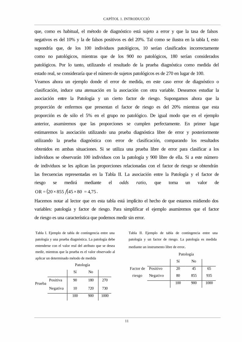
que, como es habitual, el método de diagnóstico está sujeto a error y que la tasa de falsos
negativos es del 10% y la de falsos positivos es del 20%. Tal como se ilustra en la tabla I, esto
supondría que, de los 100 individuos patológicos, 10 serían clasificados incorrectamente
como no patológicos, mientras que de los 900 no patológicos, 180 serían considerados
patológicos. Por lo tanto, utilizando el resultado de la prueba diagnóstica como medida del
estado real, se consideraría que el número de sujetos patológicos es de 270 en lugar de 100.
Veamos ahora un ejemplo donde el error de medida, en este caso error de diagnóstico o
clasificación, induce una atenuación en la asociación con otra variable. Deseamos estudiar la
asociación entre la Patología y un cierto factor de riesgo. Supongamos ahora que la
proporción de enfermos que presentan el factor de riesgo es del 20% mientras que esta
proporción es de sólo el 5% en el grupo no patológico. De igual modo que en el ejemplo
anterior, asumiremos que las proporciones se cumplen perfectamente. En primer lugar
estimaremos la asociación utilizando una prueba diagnóstica libre de error y posteriormente
utilizando la prueba diagnóstica con error de clasificación, comparando los resultados
obtenidos en ambas situaciones. Si se utiliza una prueba libre de error para clasificar a los
individuos se observarán 100 individuos con la patología y 900 libre de ella. Si a este número
de individuos se les aplican las proporciones relacionadas con el factor de riesgo se obtendrán
las frecuencias representadas en la Tabla II. La asociación entre la Patología y el factor de
riesgo se medirá mediante el odds ratio, que toma un valor de
( ) ( ) 75,4804585520OR =××= .
Hacemos notar al lector que en esta tabla está implícito el hecho de que estamos midiendo dos
variables: patología y factor de riesgo. Para simplificar el ejemplo asumiremos que el factor
de riesgo es una característica que podemos medir sin error.
Tabla I. Ejemplo de tabla de contingencia entre una
patología y una prueba diagnóstica. La patología debe
entenderse con el valor real del atributo que se desea
medir, mientras que la prueba es el valor observado al
aplicar un determinado método de medida
Patología
Sí No
Positiva 90 180 270 Prueba
Negativa 10 720 730
100 900 1000
Tabla II. Ejemplo de tabla de contingencia entre una
patología y un factor de riesgo. La patología es medida
mediante un instrumento libre de error. Patología
Sí No
Positivo 20 45 65 Factor de
riesgo Negativo 80 855 935
100 900 1000

CAPÍTOL 1. INTRODUCCIÓ
12
Ahora repitamos el ejemplo utilizando la prueba diagnóstica con error de clasificación. De los
270 individuos del grupo patológico 90 tienen realmente la enfermedad mientras que 180
están libre de ella (Tabla I). De esos 90 un 20% presentarán el factor de riesgo, es decir, 18.
En cambio, de los 180 sólo un 5% tendrán el factor de riesgo, lo que representa 9 individuos.
Esto supone que de los 270 individuos clasificados como patológicos un total de 27918 =+
presentan el factor de riesgo. ¿Qué ocurre con los 730 individuos clasificados como no
patológicos? De éstos, 10 tienen la enfermedad mientras que 720 no (Tabla I). De los 10 un
20% presentarán el factor de riesgo, es decir, 2 individuos. De los restantes 720 un 5%
tendrán el factor de riesgo, lo que supone 36 sujetos. De este modo, en el grupo de los
clasificados como no patológicos un total de 38362 =+ individuos presentarán el factor de
riesgo. Este proceso se resume en la Tabla III. Ahora el odds ratio toma un valor de
( ) ( ) 02,22433869227OR =××= , aproximadamente la mitad del valor obtenido anteriormente,
lo que significa que se ha producido una considerable atenuación de la verdadera asociación,
subestimación enteramente provocada por el error de medida de la prueba diagnóstica.
De los resultados mostrados en estos ejemplos se deduce la necesidad de valorar la calidad de
cualquier método o procedimiento de medida que utilicemos. Evaluar la calidad del
procedimiento o instrumento de medida conlleva analizar comparativamente nuestra serie de
mediciones con otra(s), las cuales pueden ser de distinto origen y características dependiendo
de los objetivos planteados en la valoración, tal y como se resume en la tabla IV .
Tabla III. Ejemplo de tabla de contingencia entre una
patología y un factor de riesgo. La patología es medida
mediante un instrumento con error
Patología
Sí No
Positivo 27 38 65 Factor de riesgo
Negativo 243 692 935
270 730 1000
Tabla IV. Clasificación de estudios para la evaluación de la calidad de los procedimientos de medida. OBJETIVOS BÁSICOS DE LA EVALUACIÓN SERIES UTILIZADAS
PARA LA COMPARACIÓN DENOMINACIÓN
DEL ESTUDIO -evaluar independencia de los errores -estimar la magnitud del error aleatorio
Valores obtenidos con el mismo procedimiento o instrumento de medida
Fiabilidad Repetibilidad
- decidir si un instrumento puede reemplazar a otro - evaluar si ambos instrumentos son intercambiables (no hay ninguna diferencia en utilizar uno u otro)
Valores obtenidos con un procedimiento o instrumento de medida alternativo
Concordancia
-cuantificar el error de medida -estimar los parámetros que han de permitir corregir el error de medida
Valores reales de la variable o atributo (p.ej. obtenidos mediante un método de referencia)
Calibración

CAPÍTOL 1. INTRODUCCIÓ
13
Cualquier comparación entre dos (o más) series de mediciones es susceptible de ser evaluada
en términos de concordancia entre las series, esto es, verificar si ambas series concuerdan (son
idénticas), o no, y en que grado, aunque el uso de esta denominación indica habitualmente que
se están analizando comparativamente dos instrumentos de medida distintos. En cualquier
caso, parece obvio que cuanto menor sea el error de medida en ambas series mayor será la
concordancia, y viceversa. En el caso extremo y poco realista de dos series sin error de
medida, su concordancia será forzosamente perfecta.
Retomando el esquema de la tabla IV, los estudios de Fiabilidad o Repetibilidad intentan
evaluar cómo concuerdan las medidas obtenidas por un único método o instrumento, utilizado
de forma repetida. Por ejemplo, podríamos utilizar varias veces un mismo analizador
automático para contar el número de CD4, procesando alícuotas de la misma muestra de
sangre, o podríamos pedir a un mismo médico que evaluase una misma imagen en varias
ocasiones. En estos casos, el aspecto que se estaría evaluando es el error de medida del
método mediante el estudio de la concordancia intra-método, de forma que si las medidas
tomadas con el mismo método concuerdan se puede declarar al método libre de error aleatorio
calificándolo de “repetible”. En los denominados estudios de Concordancia, se verifica cómo
concuerdan las medidas obtenidas por el método cuya calidad se desea valorar, con las
obtenidas por otro método. Por ejemplo, podríamos utilizar dos analizadores automáticos
distintos para contar el número de CD4 de una muestra, o podríamos pedir a dos clínicos que
valorasen una misma imagen. En estos casos estaríamos evaluando la concordancia entre
métodos de medida, con el objetivo de determinar si los dos métodos son intercambiables, de
forma que sea indiferente utilizar uno u otro. Por último, la calibración de un método de
medida es un caso particular de concordancia entre métodos. Este ensayo se realiza cuando se
comparan un procedimiento de medida con los valores reales de los sujetos. De hecho, el
valor real es imposible de determinar y en estos ensayos se comparan dos métodos de medida,
siendo uno de ellos utilizado como método de referencia o patrón (gold standard) para lo que
se asume que está libre de error de medida. En este caso, la comparación del método en
estudio con el patrón permite estimar los posibles errores, sistemáticos y aleatorio, del
primero. Una vez estimados, cualquier lectura futura obtenida con el método en estudio puede
corregirse y quedar exenta de error sistemático. Este ejercicio se conoce como calibración de
un método de medida. Lamentablemente, la naturaleza impredecible de los errores aleatorios
hace que sea imposible corregirlos, tal como se hace con los errores sistemáticos. Puesto que
los errores sistemáticos tienen arreglo (calibrando) y los aleatorios no, ambos tipos de error no
son igualmente temibles.

CAPÍTOL 1. INTRODUCCIÓ
14
En cualquier caso, la presencia de errores en las medidas es la responsable de que no exista
concordancia perfecta entre distintos instrumentos o procedimientos de medida. De hecho,
cuanto más error, menos concordancia y viceversa. Así, estudiar la concordancia es una
manera de evaluar el error de medida y por ello nos centraremos en ofrecer al lector una
panorámica de los métodos más habituales para el estudio de la misma.
En general, las técnicas para evaluar concordancia se pueden clasificar entre agregadas y
desagregadas. Los procedimientos desagregados evalúan las distintas componentes de la falta
de concordancia por separado, mientras los procedimientos agregados valoran la falta de
concordancia en global, sin distinguir entre error sistemático y error aleatorio. Una medida
agregada será útil para una evaluación rápida del grado de concordancia sin entrar en las
fuentes de error que causan la falta de concordancia. En cambio, un análisis desagregado
analizará más detalladamente las posibles fuentes de error.
Las técnicas utilizadas también variarán según la naturaleza de las variables, dependiendo de
si las medidas corresponden a una escala de medida cualitativa o cuantitativa.
Concordancia entre variables cualitativas
Supongamos que un médico realiza habitualmente una clasificación diagnóstica (positivo o
negativo) basándose en su particular apreciación de las características de una imagen
radiológica. Independientemente de cómo llega a realizar la valoración, el método de medida
es el propio médico que estaría realizando medidas en escala nominal (dicotómica). En esta
situación podría ser interesante valorar tanto el error de medida del médico (concordancia
intra-método) como la discrepancia en el diagnóstico en relación con otro profesional
(concordancia entre métodos). En ambos casos el procedimiento será similar, ya que la
primera situación es equivalente a realizar una concordancia entre diferentes mediciones
efectuadas con un único método. Veamos la situación en el caso de desear estimar la
concordancia entre dos métodos.
Los datos obtenidos de n pacientes pueden ser resumidos en una tabla de contingencia 2x2
(Tabla V).
Tabla V. Tabla de contingencia referente a las mediciones
que realizan dos evaluadores sobre una serie de
individuos.
Evaluador B
Positivo Negativo
Positivo n11 n12 Evaluador A
Negativo n21 n22
CAPÍTOL 1. INTRODUCCIÓ
15
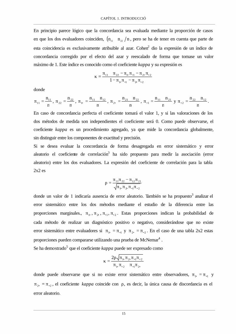
En principio parece lógico que la concordancia sea evaluada mediante la proporción de casos
en que los dos evaluadores coinciden, ( ) nnn 2211 + , pero se ha de tener en cuenta que parte de
esta coincidencia es exclusivamente atribuible al azar. Cohen2 dio la expresión de un índice de
concordancia corregido por el efecto del azar y reescalado de forma que tomase un valor
máximo de 1. Este índice es conocido como el coeficiente kappa y su expresión es
2211
22112211
1 ••••
••••
ππ−ππ−ππ−ππ−π+π
=κ
donde
nn11
11 =π , n
n 2222 =π ,
nnn 1211
1
+=π • ,
nnn 2221
2
+=π • ,
nnn 2111
1
+=π• y
nnn 1222
2
+=π• .
En caso de concordancia perfecta el coeficiente tomará el valor 1, y si las valoraciones de los
dos métodos de medida son independientes el coeficiente será 0. Como puede observarse, el
coeficiente kappa es un procedimiento agregado, ya que mide la concordancia globalmente,
sin distinguir entre los componentes de exactitud y precisión.
Si se desea evaluar la concordancia de forma desagregada en error sistemático y error
aleatorio el coeficiente de correlación3 ha sido propuesto para medir la asociación (error
aleatorio) entre los dos evaluadores. La expresión del coeficiente de correlación para la tabla
2x2 es
2121
21122211
•••• ππππππ−ππ
=ρ
donde un valor de 1 indicaría ausencia de error aleatorio. También se ha propuesto3 analizar el
error sistemático entre los dos métodos mediante el estudio de la diferencia entre las
proporciones marginales., 2121 ,,, •••• ππππ . Estas proporciones indican la probabilidad de
cada método de realizar un diagnóstico positivo o negativo, considerándose que no existe
error sistemático entre evaluadores si 11 •• π=π y 22 •• π=π . En el caso de una tabla 2x2 estas
proporciones pueden compararse utilizando una prueba de McNemar4 .
Se ha demostrado5 que el coeficiente kappa puede ser expresado como
••••
••••
ππ+ππππππρ
=κ2121
21212
donde puede observarse que si no existe error sistemático entre observadores, 11 •• π=π y
22 •• π=π , el coeficiente kappa coincide con ρ, es decir, la única causa de discordancia es el
error aleatorio.

CAPÍTOL 1. INTRODUCCIÓ
16
El coeficiente kappa puede ser generalizado para el caso en que la escala de medida tenga
más de 2 categorías. En tal caso, la expresión del coeficiente para una escala de medida
nominal de c categorías es
( )
∑
∑
=••
=••
ππ−
ππ−π=κ c
1jjj
c
1jjjjj
1
La escala de medida también puede ser ordinal, por ejemplo, una valoración de la evolución
de un paciente en la escala: “Empeora, Sigue igual, Mejora”. En esta situación, es lógico
pensar que no debe valorarse igual una discordancia “Sigue igual versus Mejora” que una
discordancia “Empeora versus Mejora”, ya que en este último caso la discordancia es más
grave. Con el objetivo de tener en cuenta esta gradación de la discordancia se introdujo el
coeficiente kappa ponderado6, de forma que se asignan distintos pesos a la discordancias de
acuerdo con la magnitud de las mismas. Por último, se ha demostrado que el coeficiente
kappa tiene una gran dependencia de la prevalencia de la patología o característica que se está
evaluando, por ello se ha considerado que no es apropiado comparar coeficientes kappa que
han sido calculados en poblaciones con distinta prevalencia de la característica en estudio7.
Ejemplo
Se aplican dos pruebas diagnósticas a un grupo de 51 pacientes cuyos resultados se resumen
en la tabla VI.
Las estimaciones de las proporciones son
3725.05119ˆ
11 ==π , 2941.05115ˆ
22 ==π , 3137.05116ˆ
12 ==π , 0196.0511ˆ
21 ==π ,
6863.051
1619ˆ1 =
+=π • , 3137.0
51151ˆ
2 =+
=π • , 3922.051
119ˆ1 =
+=π • y
6078.051
16152 =
+=π • .
Tabla VI Ejemplo de tabla de contingencia referente a los resultados de dos pruebas diagnósticas aplicadas a una serie de individuos. Prueba B
Positivo Negativo
Positivo 19 16 35 Prueba A
Negativo 1 15 16
20 31 51

CAPÍTOL 1. INTRODUCCIÓ
17
El coeficiente kappa resultante es
3828.06078.03137.03922.06863.01
6078.03137.03922.06863.02941.03725.0ˆ =⋅−⋅−
⋅−⋅−+=κ
y su intervalo de confianza es [0.1292 ; 0.6464]8. El valor del coeficiente es bastante bajo
indicando una concordancia débil entre las dos pruebas.
Si se desea realizar un análisis desagregado, en primer lugar se calcula el coeficiente de
correlación
4565.06078.03922.03137.06863.00196.03137.02941.03725.0ˆ =
⋅⋅⋅⋅−⋅
=ρ
el coeficiente de correlación indica una asociación débil entre las dos pruebas. Si se
comparan las proporciones marginales mediante un test de McNemar se rechaza la hipótesis
de homogeneidad (P<0.001), la prueba A tiende a dar mayor resultados positivos que la
prueba B. Por lo tanto, en este caso la discordancia se debe tanto a error sistemático como a
error aleatorio.
Concordancia entre variables cuantitativas
Supongamos que una característica cuantitativa se mide mediante dos métodos, X e Y, en una
serie de N individuos. Una primera aproximación exploratoria seria representar gráficamente
los dos métodos mediante un diagrama de dispersión, donde cada punto representa la pareja
de medidas obtenida de cada individuo. Si la concordancia fuera perfecta, todos los puntos se
situarían sobre la bisectriz (Y=X), tal como se muestra en la Figura 1. En esta situación es
fácil ver que la asignación del procedimiento X al eje de abcisas y el de Y al eje de ordenadas
es absolutamente arbitraria: se obtendría la misma imagen gráfica en caso de invertir la
asignación de los ejes. Observando este gráfico (Figura 1a) es fácil intuir que una medida útil
de discordancia podría basarse en la distancia de cada punto a la bisectriz. Se puede demostrar
que la media de estas distancias es proporcional a la desviación cuadrática media
( )∑=
−=n
1i
2ii YX
N1
DCM . Esta medida puede expresarse en función de las medias y las
varianzas de los resultados obtenidos con cada método y la correlación entre ambos, del
siguiente modo:
( ) ( ) ( ) YXXY
2
YX2
YX 12DCM σσρ−+σ−σ+µ−µ=
donde Xµ y Yµ representan las medias de cada método, Xσ y Yσ las desviaciones típicas y
XYρ el coeficiente de correlación de Pearson.

CAPÍTOL 1. INTRODUCCIÓ
18
La concordancia será perfecta cuando DCM=0, situación que se dará si y sólo si los tres
términos son iguales a cero. Ello implica que haya igualdad de medias (ausencia de error
sistemático constante y proporcional), YX µ=µ , igualdad de desviaciones típicas (ausencia de
error sistemático proporcional), YX σ=σ , y que la correlación sea perfecta (ausencia de error
aleatorio), 1XY =ρ . Llegados a este punto es fácil darse cuenta de que la comparación de
medias o el cálculo del coeficiente de correlación de Pearson son insuficientes para el estudio
de la concordancia. La igualdad de medias tan sólo garantiza que los dos métodos se
encuentran centrados en el mismo valor, pero en ningún caso que todos sus valores sean
iguales. Las figuras 1b y 1d representan situaciones en que hay igualdad de medias pero los
valores no concuerdan. Del mismo modo un coeficiente de correlación de 1 indica una
relación lineal perfecta, es decir, la relación entre los dos métodos es una recta carente de
error aleatorio, pero esta recta no tiene por qué ser la bisectriz (Figuras 1c y 1d) y, por tanto,
una correlación perfecta no es sinónimo de concordancia perfecta . Además la diferencia de
varianzas ha resultado ser también un componente de la concordancia, y por tanto debe
también ser evaluado.
Figura 1. Ejemplos de gráficos de dispersión de las mediciones realizadas por dos instrumentos de medida
a)
96 98 100 102 104
x
9698
100
102
104
y
b)
94 96 98 100 102 104 106
x
9496
9810
010
210
410
6
y
c)
96 98 100 102 104 106 108
x
9698
100
102
104
106
108
y
d)
96 98 100 102 104
x
9698
100
102
104
y
CAPÍTOL 1. INTRODUCCIÓ
19
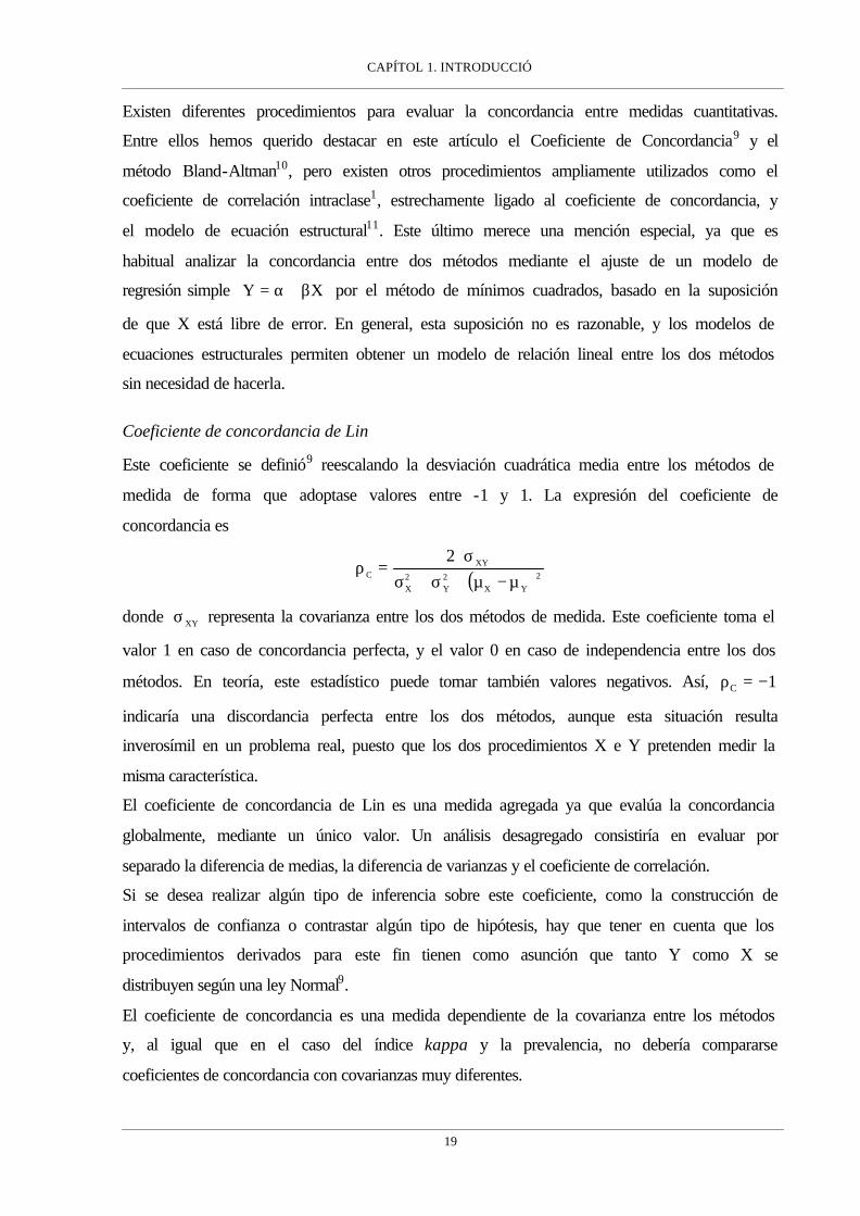
Existen diferentes procedimientos para evaluar la concordancia entre medidas cuantitativas.
Entre ellos hemos querido destacar en este artículo el Coeficiente de Concordancia9 y el
método Bland-Altman10, pero existen otros procedimientos ampliamente utilizados como el
coeficiente de correlación intraclase1, estrechamente ligado al coeficiente de concordancia, y
el modelo de ecuación estructural11. Este último merece una mención especial, ya que es
habitual analizar la concordancia entre dos métodos mediante el ajuste de un modelo de
regresión simple XY β+α= por el método de mínimos cuadrados, basado en la suposición
de que X está libre de error. En general, esta suposición no es razonable, y los modelos de
ecuaciones estructurales permiten obtener un modelo de relación lineal entre los dos métodos
sin necesidad de hacerla.
Coeficiente de concordancia de Lin
Este coeficiente se definió9 reescalando la desviación cuadrática media entre los métodos de
medida de forma que adoptase valores entre -1 y 1. La expresión del coeficiente de
concordancia es
( )2YX
2Y
2X
XYC
2µ−µ+σ+σ
σ⋅=ρ
donde XYσ representa la covarianza entre los dos métodos de medida. Este coeficiente toma el
valor 1 en caso de concordancia perfecta, y el valor 0 en caso de independencia entre los dos
métodos. En teoría, este estadístico puede tomar también valores negativos. Así, 1C −=ρ
indicaría una discordancia perfecta entre los dos métodos, aunque esta situación resulta
inverosímil en un problema real, puesto que los dos procedimientos X e Y pretenden medir la
misma característica.
El coeficiente de concordancia de Lin es una medida agregada ya que evalúa la concordancia
globalmente, mediante un único valor. Un análisis desagregado consistiría en evaluar por
separado la diferencia de medias, la diferencia de varianzas y el coeficiente de correlación.
Si se desea realizar algún tipo de inferencia sobre este coeficiente, como la construcción de
intervalos de confianza o contrastar algún tipo de hipótesis, hay que tener en cuenta que los
procedimientos derivados para este fin tienen como asunción que tanto Y como X se
distribuyen según una ley Normal9.
El coeficiente de concordancia es una medida dependiente de la covarianza entre los métodos
y, al igual que en el caso del índice kappa y la prevalencia, no debería compararse
coeficientes de concordancia con covarianzas muy diferentes.

CAPÍTOL 1. INTRODUCCIÓ
20
Método Bland-Altman
Con este procedimiento desagregado10, 12, 13, se pretende determinar si dos métodos de medida
X e Y concuerdan lo suficiente para que puedan ser declarados como intercambiables. Para
ello, se calcula, para cada individuo, la diferencia entre las medidas obtenidas con los dos
métodos (D=X-Y). La media de estas diferencias ( )dx representa el error sistemático
mientras que la varianza de estas diferencias ( )2ds mide la dispersión del error aleatorio, es
decir, la imprecisión. Se ha propuesto utilizar estas dos medidas para calcular los límites de
concordancia del 95% como dd s2x ⋅± . Estos límites nos informan entre que diferencias
oscilan la mayor parte de las medidas tomadas con los dos métodos. Naturalmente,
corresponde al investigador valorar si estas diferencias son suficientemente pequeñas como
para considerar que los dos métodos sean intercambiables, o no.
Por otro lado, para que la media y la varianza de las diferencias sean estimaciones correctas
debemos asumir que son constantes a lo largo del rango de medidas, es decir, que la magnitud
de la medida no está asociada con un error mayor. Para comprobar esta suposición se puede
construir un gráfico de dispersión, representando las diferencias (D) en el eje de ordenadas y
la media de las dos medidas de cada individuo, ( ) 2YX + en el eje de abscisas. La media de
las medidas de los dos métodos puede entenderse como una aproximación al valor real ya que
se estaría atenuando el error de medida de los dos métodos, de este modo esta representación
gráfica permite observar si existe algún tipo de relación entre la diferencia de los dos métodos
respecto a la magnitud de la medida, es decir, si el error de medida es constante a lo largo del
rango de valores de la característica que se está midiendo o, si por el contrario, el error se
incrementa conforme aumenta el valor real que se quiere medir. Asimismo es posible
representar los límites de concordancia del 95% pudiendo identificar los individuos más
discordantes.
Ejemplo
En la tabla VII se muestran los valores obtenidos por dos métodos de medida utilizados en 16
sujetos. En la figura 2a se representa las dos variables en un gráfico de dispersión. En esta
figura puede observarse que las medidas no concuerdan, tanto por error sistemático
(alejamiento de la bisectriz) como por error aleatorio (dispersión de los puntos).
Tabla VII. Ejemplo de mediciones sobre una característica cuantitativa realizadas por dos métodos de medida.
1 2 3 4 5 6 7 8 9 10 11 12 13 14 15 16
Método X 4200 3500 1900 4700 1600 3300 2400 2800 2100 2900 1800 1600 3700 2900 1200 1700
Método Y 5100 5600 3100 6700 2700 5600 5000 3100 2100 3400 1600 1800 4700 3700 3100 2800

CAPÍTOL 1. INTRODUCCIÓ
21
El análisis para evaluar la concordancia se realizará combinando tanto el coeficiente de
concordancia de Lin como el método de Bland y Altman, ya que los dos procedimientos
pueden utilizarse paralelamente en el mismo análisis.
Para ello, en necesario obtener las medias y las varianzas de cada método, la covarianza de
ambos, y la media y la desviación típica de las diferencias. En la tabla VIII se muestran estos
valores.
La estimación del coeficiente de concordancia es 0.5703 con un intervalo de confianza9 de
[0.2892 ; 0.7609], indicando un bajo grado de concordancia.
Los límites de concordancia de Bland-Altman son 6007,733166*25,1112 −=− y
28257,733166*25,1112 =+ . Éstos se representan el gráfico de Bland-Altman de la Figura
2b, donde puede observarse que la diferencia entre los dos métodos tiene una tendencia lineal
positiva, esto es, la diferencia se incrementa con la magnitud de la medida. Este hecho es
indicativo de un error sistemático proporcional que puede ser estimado mediante el cociente
de desviaciones típicas 47.110572922291958ss XY == .
Este resultado se interpreta del siguiente modo: el método Y toma sistemáticamente valores
superiores al método X en una proporción de 1,47. El coeficiente de correlación es de 0.8402,
indicando un grado de correlación elevado. Por lo tanto la principal fuente de discordancia
entre los dos métodos es el error sistemático.
Tabla VIII. Medias, varianzas y covarianza de las mediciones
realizadas por los dos métodos de medida y su diferencia.
Método Media Varianza Covarianza
X 2643,75 1057292
Y 3756,25 2291958 1308042
D = Y-X 1112,5 733166,7
Figura 2. Gráfico de dispersión y gráfico Diferencia versus Media relacionados con los instrumentos de medida del
ejemplo
a)
0 2000 4000 6000
Método X
020
0040
0060
00
Mét
odo
Y
b)
1000 2000 3000 4000 5000 6000
Media
-300
0-2
000
-100
00
1000
2000
3000
Dife
renc
ia

CAPÍTOL 1. INTRODUCCIÓ
22
Discusión
La calidad de las medidas es fundamental en cualquier ámbito, pero adquiere un especial
interés en el campo de las Ciencias de la Salud14,15,16, donde continuamente se toman
decisiones basadas en mediciones. Esto implica que el acierto en las decisiones depende de la
calidad de dichas mediciones. Es tentador dar por supuesto que los métodos de medida que
utilizamos son buenos y que los resultados que nos proporcionan son correctos y fiables. Si
una glucemia en ayunas es de 129 mg/dl se diagnóstica al paciente como diabético, pero
¿quién nos asegura que realmente este paciente tiene tal concentración de glucosa en sangre?
Es más, si se repite la determinación en otro laboratorio, ¿se obtendrá el mismo resultado?
Estas preguntas sólo pueden responderse mediante ensayos de fiabilidad y concordancia de
las medidas.
La falta de concordancia puede deberse a dos tipos de error: sistemático y/o aleatorio.
Mientras que el error sistemático puede corregirse (por calibración), para disminuir el error
aleatorio es necesario estudiar sus posibles causas e intentar controlar algunas de ellas en
nuevas versiones más perfeccionadas del método o aparato de medida.
Referencias
1. Fleiss JL. The Design and Analysis of Clinical Experiments. New York: Wiley, 1986 2. Cohen, J. A coefficient of agreement for nominal scales. Educational and Psychological Measurements 1960; 20; 37-46 3. Shoukri MM. Measurement of agreement. En Armitage P, Colton T, editors. Encyclopedia of biostatistics. Chichester: Wiley & Sons , 1998; p.103-17 4. Agresti A. An Introduction to Categorical Data Analys. New York: Wiley & Sons, 1996 5. Shoukri MM, Martin SW, Mian IUH. Maximum likelihood estimation of the kappa coefficient from models of matched binary responses. Statistics in Medicine 1995; 14; 83-99 6. Cohen J. Weighted kappa: nominal scale agreement with provisions for scaled disagreement or partial credit. Psychological bulletin 1968; 70; 213-220 7. Thompson WD, Walter SD. A reappraisal of the kappa coefficient. Journal of Clinical Epidemiology, 1988; 41; 969-970. 8. Shoukri MM, Pause CA. Statistical Methods for Health Sciences 2nd edition. Boca Ratón: CRC Press, 1999 9. Lin L. A concordance correlation coefficient to evaluate reproducibility. Biometrics. 1989; 45; 255-268. 10. Bland JM, Altman DG. Statistical methods for assessing agreement between two methods of clinical measurement. The Lancet 1986;l 1:8476;307-10 11. Kelly GE. Use of the structural equations model in assessing the reliability of a new measurement technique. Applied Statistics 1985; 34(3):258-263 12. Bland JM, Altman DG. Comparing methods of measurement: why plotting difference against standard methods is misleading. The Lancet 1995; 346; 1085-1087 13. Bland JM, Altman DG. Measuring agreement in method comparison studies. Statistical Methods in Medical Research 1999; 135-160. 14. Andersson SW, Niklasson A, Lapidus L, Hallberg L, Bengtsson C, Hulthén L. Poor agreement between self-reported birth weight and birth weight from original records in adult women. American Journal of Epidemiology 2000; 152:7; 609-616. 15. Schisterman EF, Faraggi D, Reiser B, Trevisan M. Statistical inference for the are under the receiver operating characteristic curve in the presence of random measurement error. American Journal of Epidemiology 2001; 154:2; 174-179 16. White E. Design and interpretation of studies of differential exposure measurement error. American Journal of Epidemiology 2003; 157:5; 380-387.

CAPÍTOL 2

CAPÍTOL 2. EL COEFICIENT DE CONCORDANÇA
25
EL COEFICIENT DE CONCORDANÇA
Introducció
En aquest capítol s’analitzen dos procediments agregats per avaluar la concordança com són
el coeficient de concordança (Lin, 1989) i el coeficient de correlació intraclasse (Fleiss,
1986). En el primer article que composa aquest capítol els dos coeficients són comparats,
arribant-se a la conclusió de que són dues expressions d’un mateix índex, les quals es
diferencien en el mètode d’estimació. Donat que el coeficient de correlació intraclasse té
diferents expressions variant segons el model de mesura subjacent, aquest fet porta a la
conclusió de que el coeficient de concordança és un coeficient de correlació intraclasse en
particular, concretament aquell basat en un model lineal mixt on els individus o clusters són
considerats un efecte aleatori mentre que els mètodes de mesura són un efecte fix, però que
intervenen en el coeficient de correlació intraclasse mitjançant una suma de quadrats. Aquest
resultat és el que ha fet que el capítol es tituli “el Coeficient de Concordança” i no es
mencioni el coeficient de correlació intraclasse perquè el mateix coeficient de concordança ha
de ser interpretat com un coeficient de correlació intraclasse.
En el segon article s’analitza el comportament del coeficient de concordança quan les dades
són recomptes. En aquest sentit s’ha comparat el coeficient de concordança estimat mitjançant
un model lineal generalitzat mixt enfront de l’obtingut amb un model lineal mixt clàssic tant
amb les dades originals com transformades per normalitzar-les.

CAPÍTOL 2. EL COEFICIENT DE CONCORDANÇA
26
Estimating The Generalized Concordance Correlation Coefficient
Through Variance Components
Josep L. Carrasco and Lluís Jover
Bioestadística, Departament de Salut Pública, Universitat de Barcelona.
Facultat de Medicina. Casanova, 143 08036 Barcelona, Spain
e-mail. [email protected]
SUMMARY
The intraclass correlation coefficient (ICC) and the concordance correlation coefficient (CCC)
are two of the most popular measures of agreement for variables measured on a continuous
scale. Here we demonstrate that ICC and CCC are the same measure of agreement estimated
in two ways: variance components and moment method procedures. We propose to estimate
the CCC using variance components of a mixed effects model instead of the common method
of moments. With the variance components approach the CCC can easily be extended to more
than two observers and adjusted using confounding covariates by incorporating them in the
mixed model. A simulation study is carried out to compare the variance components approach
with the moment method. The importance of adjusting by confounding covariates is
illustrated through a case example.
KEYWORDS: Agreement; Concordance correlation coefficient; Variance components;
Intraclass correlation coefficient; Mixed effects model.
CAPÍTOL 2. EL COEFICIENT DE CONCORDANÇA
27
1. Introduction
Agreement between continuous data measured from different measurement methods has
received a great deal of attention from the scientific community. The measurement methods
can be multiple systems, processes, machines or raters, but for the sake of simplicity we refer
to them as observers throughout the paper. A simple way to classify the procedures which
measure agreement is to differentiate between aggregate and disaggregate approaches, where
a disaggregate approach evaluates agreement for each component of the measurement model
separately, for example, difference of means or error variances. An example of a disaggregate
procedure is the structural equation model (Cheng and Van Ness, 1999; Kelly, 1985).
On the other hand, an aggregate approach assesses agreement using a single measure as a
concordance magnitude. The intraclass correlation coefficient (Pearson, 1901) and the
concordance correlation coefficient (Lin, 1989) are two of the most popular aggregate
procedures used to measure agreement when data are on a continuous scale.
The intraclass correlation coefficient (ICC) measures the amount of overall data variance due
to between-subjects variability, while the concordance correlation coefficient (CCC) was
defined by Lin (1989) based on the distance on the plane of each pair of data to the 45º line
through the origin. The CCC has components of precision and accuracy. The disaggregate
approach can also be evaluated by assessing the precision and accuracy components
separately (Lin et al, 2002).
Since the ICC is defined using variance components, several expressions of ICC can be found
(Bartko, 1966; Shrout and Fleiss, 1979) depending on the measurement model chosen. The
ICC usually comes from a 2-way analysis of variance where observers and subjects are
considered as effects. But at the same time, this dependence of the ICC expression on the
measurement model causes some confusion. Thus, the ICC was criticized as a measure of
agreement among observers for two reasons: first, it allows duplicate readings to be
interchangeable (Lin, 1989; Barnhart and Williamson, 2001), that is, it cannot measure lack of
accuracy (difference of means) between observers measures; and second, it gives a negative
value when the paired readings are uncorrelated (Lin, 1989). We will argue that the ICC is a
valid measure of agreement among observers and it can indeed take into account the
difference of observer means if it is suitably expressed.
The CCC is another, widely used agreement measure (Lin, 1992; Calderone and Turcotte,
1998; Ruel et al., 1997; Singh and Jones, 2002) and it is interesting to note the differences and
similarities between the coefficients. For the case of two observers, Nickerson (1997) found

CAPÍTOL 2. EL COEFICIENT DE CONCORDANÇA
28
them practically identical, and Robieson (1999) found them to be asymptotically equivalent.
Furthermore, a CCC for more than two observers is required (Lin, 1989; King and Chinchilli,
2001; Barnhart, Haber and Song, 2002) and, moreover, the CCC needs to be adjusted by
confounding covariates (Barnhart and Williamson, 2001; King and Chinchilli, 2001). As a
result of the comparison between the CCC and ICC we will show that it is simple to adjust the
CCC by covariates and obtain a CCC for more than two observers.
The paper is structured as follows: in section 2, the ICC and CCC are defined and compared.
Section 3 contains the extension of CCC to more than two observers, the covariate-adjusted
CCC, and some inference questions. In section 4, moment-method and variance components
procedures of CCC estimation are compared through a simulation study. Section 5 shows a
case-example involving the agreement between a manual and an automatic blood pressure
device. In this example, the need for confounding covariate adjustment is illustrated through
the inclusion of sex, age and heart rate in the CCC estimation. Finally, the discussion and
conclusions are included in section 6.
2. Comparison of CCC and ICC
2.1 Concordance Correlation Coefficient
Lin (1989) defined the CCC for two observers assuming data was distributed under a bivariate
normal distribution, therefore ( ) ( )Σ,MVN~Y,Y 21 µ where Y1 and Y2 are the array of
measurements of each observer, ( )21 ,µµ=µ is the vector of the observer means and
σσσσ
=2212
1221S
is the covariance matrix.
Lin based the CCC on the distance between Y1 and Y2 in relation to the concordance point.
He used the expectation of the square difference, defining the CCC as
( ){ }( ){ } ( )2
2122
21
12
212
21
221
C
2eduncorrelat are Y and Ywhen YYE
YYE1
µ−µ+σ+σσ⋅
=−
−−=ρ .
To build confidence intervals Lin (1989) suggests using the inverse hyperbolic tangent
transformation or Z-transformation, ( ) ( ) ( ){ }CCC1
C 11ln5.0tanhZ ρ−ρ+⋅=ρ= − , which
improves the approximation to a Gaussian distribution. The standard error expression of CZ
was provided by Lin (1989, 2000), so the confidence interval estimation is made through the
confidence interval of CZ , which is built using a standard normal distribution.
CAPÍTOL 2. EL COEFICIENT DE CONCORDANÇA
29
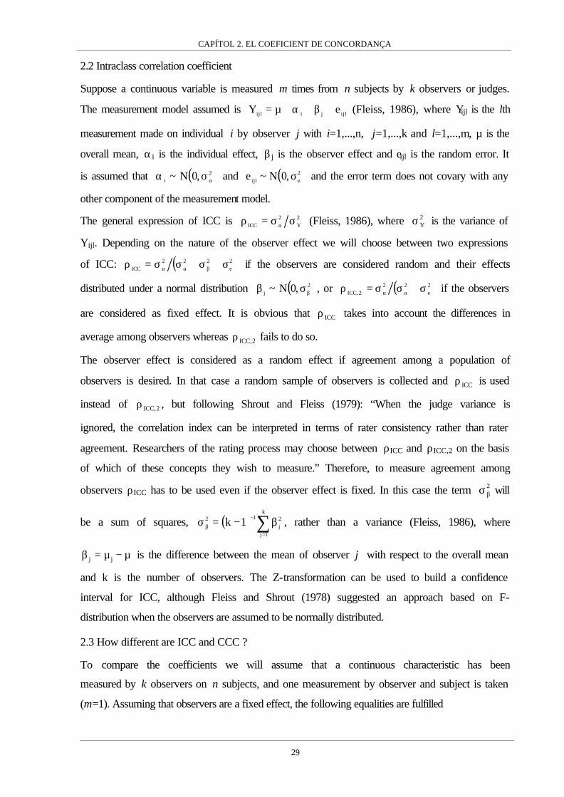
2.2 Intraclass correlation coefficient
Suppose a continuous variable is measured m times from n subjects by k observers or judges.
The measurement model assumed is ijljiijl eY +β+α+µ= (Fleiss, 1986), where Yijl is the lth
measurement made on individual i by observer j with i=1,...,n, j=1,...,k and l=1,...,m, µ is the
overall mean, αi is the individual effect, β j is the observer effect and eijl is the random error. It
is assumed that ( )2i ,0N~ ασα and ( )2
eijl ,0N~e σ and the error term does not covary with any
other component of the measurement model.
The general expression of ICC is 2Y
2ICC σσ=ρ α (Fleiss, 1986), where 2
Yσ is the variance of
Yijl. Depending on the nature of the observer effect we will choose between two expressions
of ICC: ( )2e
222ICC σ+σ+σσ=ρ βαα if the observers are considered random and their effects
distributed under a normal distribution ( )2j ,0N~ βσβ , or ( )2
e22
2,ICC σ+σσ=ρ αα if the observers
are considered as fixed effect. It is obvious that ICCρ takes into account the differences in
average among observers whereas 2,ICCρ fails to do so.
The observer effect is considered as a random effect if agreement among a population of
observers is desired. In that case a random sample of observers is collected and ICCρ is used
instead of 2,ICCρ , but following Shrout and Fleiss (1979): “When the judge variance is
ignored, the correlation index can be interpreted in terms of rater consistency rather than rater
agreement. Researchers of the rating process may choose between ρICC and ρICC,2 on the basis
of which of these concepts they wish to measure.” Therefore, to measure agreement among
observers ρICC has to be used even if the observer effect is fixed. In this case the term 2βσ will
be a sum of squares, ( ) ∑=
−
β β−=σk
1j
2j
12 1k , rather than a variance (Fleiss, 1986), where
µ−µ=β jj is the difference between the mean of observer j with respect to the overall mean
and k is the number of observers. The Z-transformation can be used to build a confidence
interval for ICC, although Fleiss and Shrout (1978) suggested an approach based on F-
distribution when the observers are assumed to be normally distributed.
2.3 How different are ICC and CCC ?
To compare the coefficients we will assume that a continuous characteristic has been
measured by k observers on n subjects, and one measurement by observer and subject is taken
(m=1). Assuming that observers are a fixed effect, the following equalities are fulfilled

CAPÍTOL 2. EL COEFICIENT DE CONCORDANÇA
30
( )∑∑−
= +=α σ
−⋅=σ
1k
1i
k
1ijij
2
1kk2
;
( ) ( )∑∑−
= +=β µ−µ
−⋅=σ
1k
1i
k
1ij
2
ji2
1kk1
and
( ) ( ) ( )∑∑∑∑∑−
= +==
−
= +=
σ−⋅
−σ=σ−σ+σ−⋅
=σ1k
1i
k
1ijij
k
1i
2i
1k
1i
k
1ijij
2j
2i
2e 1kk
2k1
221
1kk2
where 2iσ and iµ are the variance and mean of the measurements made by observer i, and ijσ
is the covariance between the measurements from observers i and j. Thus, the ICC can be
expressed in terms of the variances, covariances and means of the observers measurements
( ) ( )∑∑∑
∑∑−
= +==
−
= +=
βα
α
µ−µ+σ−
σ=
σ+σ+σσ
=ρ 1k
1i
k
1ij
2
ji
k
1i
2i
1k
1i
k
1ijij
2e
22
2
ICC
1k
2
which is exactly the same expression as the overall concordance correlation coefficient for k
observers suggested in the works of Lin (1989), King and Chinchilli (2001) and Barnhart et
al. (2002). Hence, the concordance correlation coefficient is the intraclass correlation
coefficient when the observers are considered as a fixed effect.
This result implies that CCC can be estimated by variance components through a mixed
effects model easily generalizable to more than two observers.
Although the concordance correlation coefficient is no more than a particular intraclass
correlation coefficient, throughout the paper we will refer to it as concordance correlation
coefficient.
3. Concordance correlation coefficient estimated by variance components
3.1 Estimation of the CCC for k observers
CCC could be estimated either using variance components estimation methods (Searle,
Casella and McCulloch, 1992) or by estimating the variances, covariances and means of the
observer measurements following Lin (1989).
Suppose 2iS , iY and ijS are the unbiased estimators of 2
iσ , iµ and ijσ respectively. If these
estimates are used to estimate the components of CCC and their expectations are taken, we
reach
( ) ( )∑∑∑∑−
= +=
−
= +=
σ−⋅
=
−⋅
1k
1i
k
1ijij
1k
1i
k
1ijij 1kk
2S
1kk2
E
CAPÍTOL 2. EL COEFICIENT DE CONCORDANÇA
31
∑∑==
σ=
k
1i
2i
k
1i
2j k
1S
k1
E
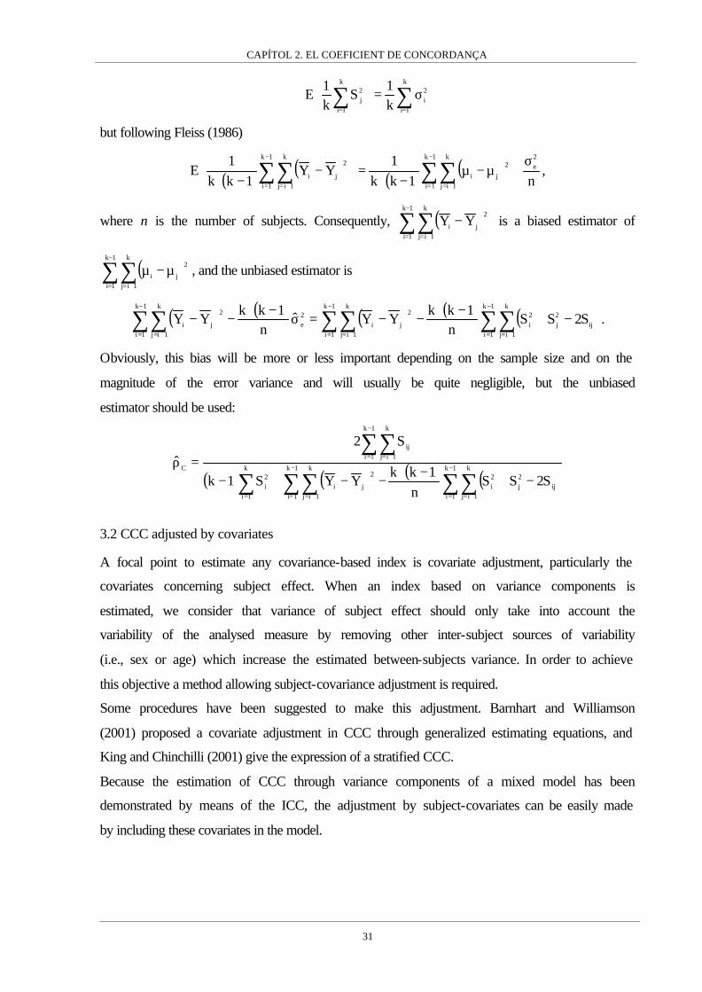
but following Fleiss (1986)
( ) ( ) ( ) ( )n1kk
1YY
1kk1
E2e
1k
1i
k
1ij
2
ji
1k
1i
k
1ij
2
ji
σ+µ−µ
−⋅=
−
−⋅ ∑∑∑∑−
= +=
−
= +=
,
where n is the number of subjects. Consequently, ( )∑∑−
= +=
−1k
1i
k
1ij
2
ji YY is a biased estimator of
( )∑∑−
= +=
µ−µ1k
1i
k
1ij
2
ji , and the unbiased estimator is
( ) ( ) ( ) ( ) ( )∑∑∑∑∑∑−
= +=
−
= +=
−
= +=
−+−⋅
−−=σ−⋅
−−1k
1i
k
1ijij
2j
2i
1k
1i
k
1ij
2
ji2e
1k
1i
k
1ij
2
ji S2SSn
1kkYYˆ
n1kk
YY .
Obviously, this bias will be more or less important depending on the sample size and on the
magnitude of the error variance and will usually be quite negligible, but the unbiased
estimator should be used:
( ) ( ) ( ) ( )∑∑∑∑∑
∑∑−
= +=
−
= +==
−
= +=
−+−⋅
−−+−=ρ 1k
1i
k
1ijij
2j
2i
1k
1i
k
1ij
2
ji
k
1i
2i
1k
1i
k
1ijij
C
S2SSn
1kkYYS1k
S2ˆ
3.2 CCC adjusted by covariates
A focal point to estimate any covariance-based index is covariate adjustment, particularly the
covariates concerning subject effect. When an index based on variance components is
estimated, we consider that variance of subject effect should only take into account the
variability of the analysed measure by removing other inter-subject sources of variability
(i.e., sex or age) which increase the estimated between-subjects variance. In order to achieve
this objective a method allowing subject-covariance adjustment is required.
Some procedures have been suggested to make this adjustment. Barnhart and Williamson
(2001) proposed a covariate adjustment in CCC through generalized estimating equations, and
King and Chinchilli (2001) give the expression of a stratified CCC.
Because the estimation of CCC through variance components of a mixed model has been
demonstrated by means of the ICC, the adjustment by subject-covariates can be easily made
by including these covariates in the model.

CAPÍTOL 2. EL COEFICIENT DE CONCORDANÇA
32
3.3 Inference about CCC
The CCC will be estimated using variance components of a mixed model with subjects as
random effect and observers as fixed effect. Although Cρ follows an asymptotic normal
distribution (Lin, 1989), in order to build a (1-α)% confidence interval the inverse hyperbolic
tangent transformation ( ) ( ) ( ){ }CCC1
Cˆ1ˆ1ln5.0ˆtanhZ ρ−ρ+=ρ= − can be used to accelerate
the convergence to a normal distribution. In this case, first the confidence interval of CZ will
be estimated and then the hyperbolic tangent transformation will be applied to obtain a
confidence interval for Cρ .
The standard error of CZ and Cρ are approximated using the Delta method (see Appendix),
then ( )CˆVar ρ expression is
( ) ( ) ( ) ( ) ( ){ }[ ] ( ) ( ) ( ){ }[ ]( )22
e22
2e
222CC
22e
2e
22C
22
C ,cov,cov12,cov2VarVarVar1
σ+σ+σ
σσ+σσ⋅ρ⋅ρ−⋅−σσ+σ+σ⋅ρ+σ⋅ρ−
βα
αβαββα
and
( ) ( )( ) ( )2
C
2
C
CC 11
ˆVarZVar
ρ−⋅ρ+ρ
≈ .
The expressions of the standard errors of variance components depend on the estimation
method. Usually this method will be a likelihood-based method such as maximum likelihood
or restricted maximum likelihood. Then the variances and covariances of parameters will be
approximated by the inverse of Fisher’s information matrix except for the case of 2βσ when
the observers are considered as a fixed effect. Here, the standard error can be approximated by
(see Appendix)
( ) ( ) ( ) ( ){ } ( )( )2
2e
1k
1i
k
1ijji
2
ji22
2
mn
ˆVarYYVarYY
1kk4ˆVar
⋅σ
+−⋅−−⋅
≈σ ∑∑−
= +=β .
For more details relating to methods of estimation for mixed effects models we address the
reader to Searle et al. (1992).
Fleiss and Shrout (1978) give the expression of a confidence interval for ICC based on the F-
distribution when the observers are considered as a random effect. This approach can also be
used to make inferences about CCC. The ( )%1 α− confidence interval will be provided by
( )( ){ }
( )( ) ( )2
e2
*2e
2
2e
2
C2e
22e
2*
2e
2
kF1kk1FFk
k1kkFF1k
σ+σ⋅+σ⋅−+σ⋅σ⋅−+σ⋅
<ρ<σ+σ⋅+σ⋅−+σ⋅
σ⋅−+σ⋅
αβ
∗α∗
αβ
∗α
where ∗F and ∗F are the ( )21 α− % percentiles of an F distribution with ( )ν− ,1n and ( )1n, −ν
degrees of freedom, respectively. Where
CAPÍTOL 2. EL COEFICIENT DE CONCORDANÇA
33
( ) ( ) ( ){ }[ ]( ) ( ){ }[ ]2
ICCICC2r
2ICC
2
2ICCICCrICC
ˆkˆ1k1nFˆk1nˆkˆ1k1nFˆk1n1k
ρ⋅−ρ⋅−+⋅+⋅ρ⋅⋅−ρ⋅−ρ⋅−+⋅+⋅ρ⋅⋅−⋅−
=ν
and ( )2e
2r
ˆˆn1F σσ⋅+= β
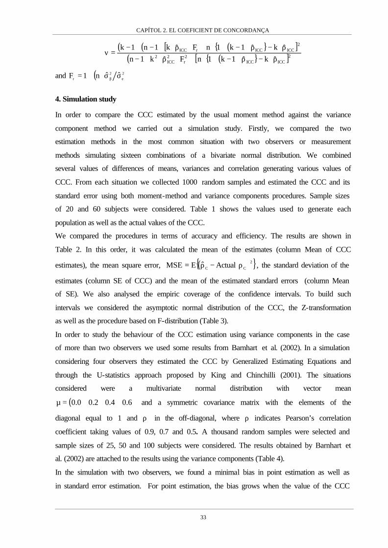
4. Simulation study
In order to compare the CCC estimated by the usual moment method against the variance
component method we carried out a simulation study. Firstly, we compared the two
estimation methods in the most common situation with two observers or measurement
methods simulating sixteen combinations of a bivariate normal distribution. We combined
several values of differences of means, variances and correlation generating various values of
CCC. From each situation we collected 1000 random samples and estimated the CCC and its
standard error using both moment-method and variance components procedures. Sample sizes
of 20 and 60 subjects were considered. Table 1 shows the values used to generate each
population as well as the actual values of the CCC.
We compared the procedures in terms of accuracy and efficiency. The results are shown in
Table 2. In this order, it was calculated the mean of the estimates (column Mean of CCC
estimates), the mean square error, ( ){ }2
CC ActualˆEMSE ρ−ρ= , the standard deviation of the
estimates (column SE of CCC) and the mean of the estimated standard errors (column Mean
of SE). We also analysed the empiric coverage of the confidence intervals. To build such
intervals we considered the asymptotic normal distribution of the CCC, the Z-transformation
as well as the procedure based on F-distribution (Table 3).
In order to study the behaviour of the CCC estimation using variance components in the case
of more than two observers we used some results from Barnhart et al. (2002). In a simulation
considering four observers they estimated the CCC by Generalized Estimating Equations and
through the U-statistics approach proposed by King and Chinchilli (2001). The situations
considered were a multivariate normal distribution with vector mean
( )6.04.02.00.0=µ and a symmetric covariance matrix with the elements of the
diagonal equal to 1 and ρ in the off-diagonal, where ρ indicates Pearson’s correlation
coefficient taking values of 0.9, 0.7 and 0.5. A thousand random samples were selected and
sample sizes of 25, 50 and 100 subjects were considered. The results obtained by Barnhart et
al. (2002) are attached to the results using the variance components (Table 4).
In the simulation with two observers, we found a minimal bias in point estimation as well as
in standard error estimation. For point estimation, the bias grows when the value of the CCC
CAPÍTOL 2. EL COEFICIENT DE CONCORDANÇA
34
decreases and the bias is systematically greater in moment-method (MM) than in variance
components (VC) confirming the bias of the MM estimator proposed by Lin (1989).
Both procedures give accurate estimates of the standard error with the exception of the MM
method when there is a difference of means and the correlation is 0.99. In this case the MM
method fails and gives a standard error mean between 54.9% and 70.4% of the actual standard
error. Regarding the variability of the estimates (SE of CCC in table 2), the standard error of
the estimates is systematically greater in the MM than the VC approach.
The coverage of the confidence intervals is correct compared to nominal coverage but we
must highlight combinations 9 and 13, where the MM approach fails to achieve the desirable
coverage. This is linked to the fact that in these combinations the moment method
underestimates the standard error.
Despite the fact that the coverage is correct with the asymptotic approach, the Z-
transformation gives more accurate and steady coverage. The confidence intervals based on F
approximations work quite well when there is no difference of means but when this
component of variance appears, the F-approximation overestimates the nominal coverage.
In the simulation with more than two observers, there is a bias in GEE and U-statistics. This
may be attributable to the use of the CCC biased estimator (section 2). Standard errors are
estimated with more precision in the variance components method, which improves coverage
of confidence intervals in most combinations simulated.
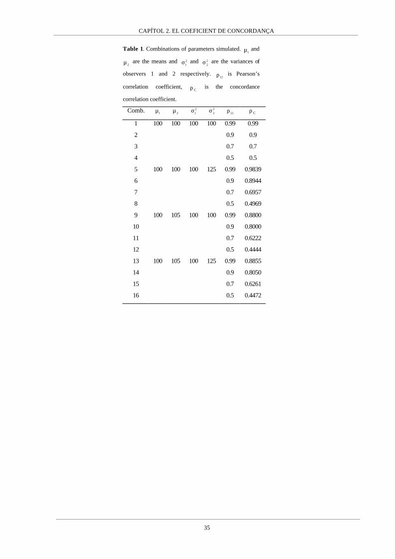
CAPÍTOL 2. EL COEFICIENT DE CONCORDANÇA
35
Table 1. Combinations of parameters simulated. 1µ and
2µ are the means and 21σ and 2
2σ are the variances of
observers 1 and 2 respectively. 12ρ is Pearson’s
correlation coefficient, Cρ is the concordance
correlation coefficient.
Comb. 1µ 2µ 2
1σ 22σ
12ρ Cρ
1 100 100 100 100 0.99 0.99
2 0.9 0.9
3 0.7 0.7
4 0.5 0.5
5 100 100 100 125 0.99 0.9839
6 0.9 0.8944
7 0.7 0.6957
8 0.5 0.4969
9 100 105 100 100 0.99 0.8800
10 0.9 0.8000
11 0.7 0.6222
12 0.5 0.4444
13 100 105 100 125 0.99 0.8855
14 0.9 0.8050
15 0.7 0.6261
16 0.5 0.4472

CAPÍTOL 2. EL COEFICIENT DE CONCORDANÇA
36
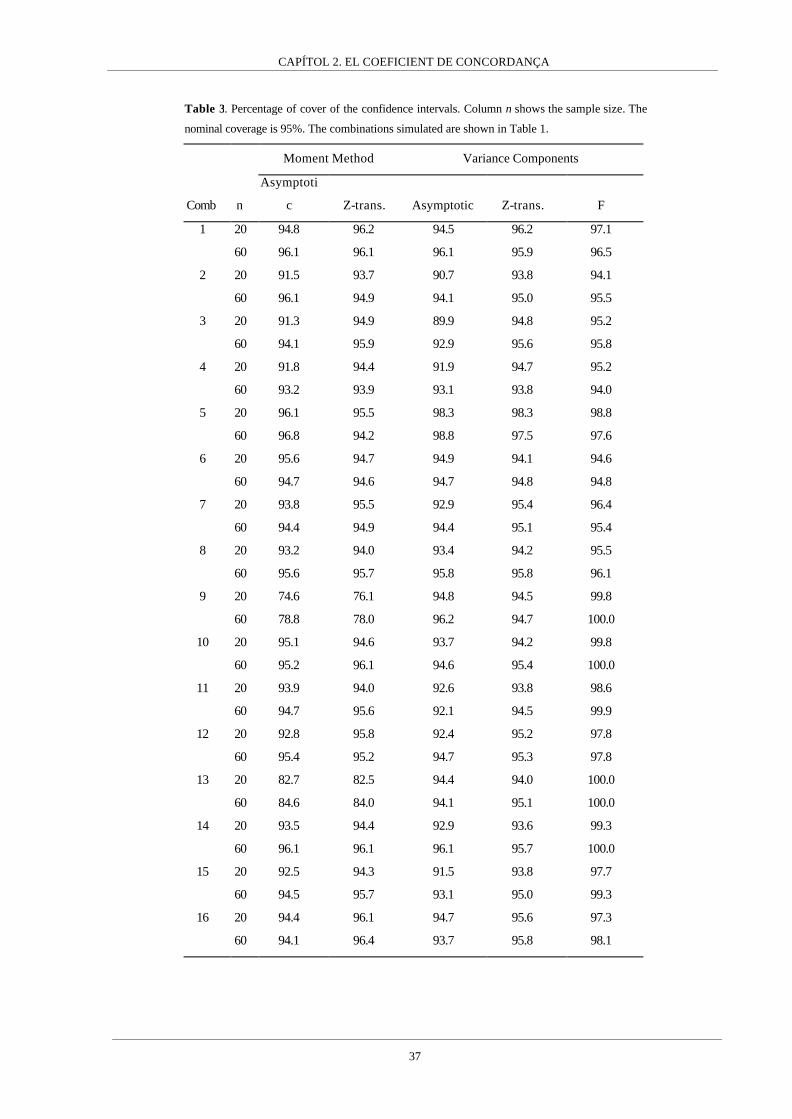
CAPÍTOL 2. EL COEFICIENT DE CONCORDANÇA
37
Table 3. Percentage of cover of the confidence intervals. Column n shows the sample size. The
nominal coverage is 95%. The combinations simulated are shown in Table 1.
Moment Method Variance Components
Comb n
Asymptoti
c Z-trans. Asymptotic Z-trans. F
20 94.8 96.2 94.5 96.2 97.1 1
60 96.1 96.1 96.1 95.9 96.5
20 91.5 93.7 90.7 93.8 94.1 2
60 96.1 94.9 94.1 95.0 95.5
20 91.3 94.9 89.9 94.8 95.2 3
60 94.1 95.9 92.9 95.6 95.8
20 91.8 94.4 91.9 94.7 95.2 4
60 93.2 93.9 93.1 93.8 94.0
20 96.1 95.5 98.3 98.3 98.8 5
60 96.8 94.2 98.8 97.5 97.6
20 95.6 94.7 94.9 94.1 94.6 6
60 94.7 94.6 94.7 94.8 94.8
20 93.8 95.5 92.9 95.4 96.4 7
60 94.4 94.9 94.4 95.1 95.4
20 93.2 94.0 93.4 94.2 95.5 8
60 95.6 95.7 95.8 95.8 96.1
20 74.6 76.1 94.8 94.5 99.8 9
60 78.8 78.0 96.2 94.7 100.0
20 95.1 94.6 93.7 94.2 99.8 10
60 95.2 96.1 94.6 95.4 100.0
20 93.9 94.0 92.6 93.8 98.6 11
60 94.7 95.6 92.1 94.5 99.9
20 92.8 95.8 92.4 95.2 97.8 12
60 95.4 95.2 94.7 95.3 97.8
20 82.7 82.5 94.4 94.0 100.0 13
60 84.6 84.0 94.1 95.1 100.0
20 93.5 94.4 92.9 93.6 99.3 14
60 96.1 96.1 96.1 95.7 100.0
20 92.5 94.3 91.5 93.8 97.7 15
60 94.5 95.7 93.1 95.0 99.3
20 94.4 96.1 94.7 95.6 97.3 16
60 94.1 96.4 93.7 95.8 98.1

CAPÍTOL 2. EL COEFICIENT DE CONCORDANÇA
38
Table 4. Results of the simulations for more than two observers.
True ρ True ρC Sample size Method Mean S.D. Mean S.E.
95%
coverage
(%)*
95%
coverage
(%)**
0.5 0.469 100 GEE 0.464 0.0517 0.0492 93.8
U-Stat 0.464 0.0517 0.0491 93.8
VC 0.473 0.0477 0.0502 95.9 96.1
50 GEE 0.459 0.0702 0.0679 93.1
U-Stat 0.459 0.0702 0.0679 93.1
VC 0.465 0.0746 0.0709 92.6 93.7
25 GEE 0.449 0.1001 0.0906 89.5
U-Stat 0.449 0.1001 0.0904 89.4
VC 0.462 0.1003 0.1001 92.9 94.1
0.7 0.656 100 GEE 0.651 0.0410 0.0398 93.1
U-Stat 0.651 0.0410 0.0398 93.2
VC 0.659 0.0380 0.0398 94.8 95.3
50 GEE 0.646 0.0580 0.0549 92.3
U-Stat 0.646 0.0580 0.0550 92.4
VC 0.652 0.0605 0.057 92.6 92.2
25 GEE 0.635 0.0841 0.0753 90.4
U-Stat 0.635 0.0841 0.0756 90.5
VC 0.646 0.0844 0.0815 93.6 93.8
0.9 0.844 100 GEE 0.840 0.0226 0.0211 92.4
U-Stat 0.840 0.0226 0.0216 92.7
VC 0.844 0.0210 0.0211 95.0 95.5
50 GEE 0.836 0.0315 0.0300 93.9
U-Stat 0.836 0.0315 0.0307 94.2
VC 0.840 0.0339 0.0308 92.7 92.5
25 GEE 0.828 0.0498 0.0419 91.2
U-Stat 0.828 0.0498 0.0428 91.6
VC 0.837 0.0466 0.0449 94.0 94.0 * Using ( )CC
ˆ.E.S96.1ˆ ρ⋅±ρ
** Using the Z-transformation
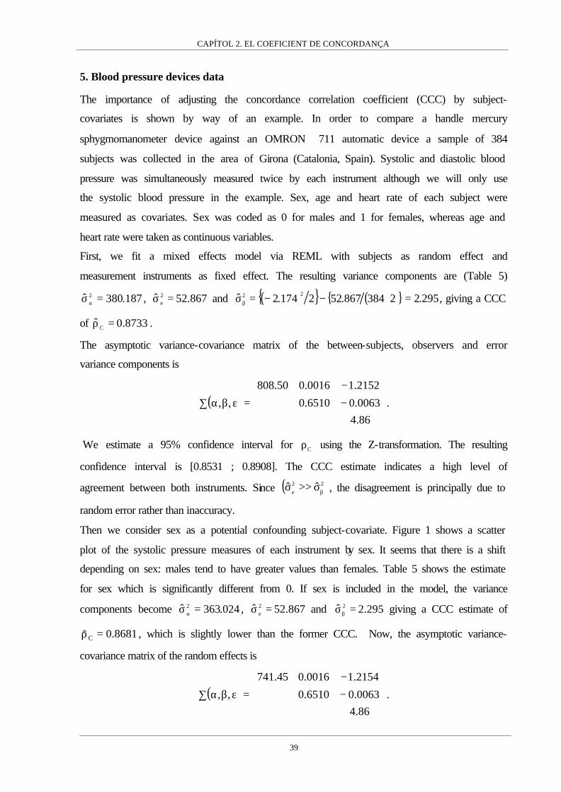
CAPÍTOL 2. EL COEFICIENT DE CONCORDANÇA
39
5. Blood pressure devices data
The importance of adjusting the concordance correlation coefficient (CCC) by subject-
covariates is shown by way of an example. In order to compare a handle mercury
sphygmomanometer device against an OMRON 711 automatic device a sample of 384
subjects was collected in the area of Girona (Catalonia, Spain). Systolic and diastolic blood
pressure was simultaneously measured twice by each instrument although we will only use
the systolic blood pressure in the example. Sex, age and heart rate of each subject were
measured as covariates. Sex was coded as 0 for males and 1 for females, whereas age and
heart rate were taken as continuous variables.
First, we fit a mixed effects model via REML with subjects as random effect and
measurement instruments as fixed effect. The resulting variance components are (Table 5)
187.380ˆ 2 =σα , 867.52ˆ 2e =σ and ( ){ } ( ){ } 295.22384867.522174.2ˆ 22 =⋅−−=σβ , giving a CCC
of 8733.0ˆC =ρ .
The asymptotic variance-covariance matrix of the between-subjects, observers and error
variance components is
( )
−
−
=εβα∑86.40063.06510.0
2152.10016.050.808
,, .
We estimate a 95% confidence interval for Cρ using the Z-transformation. The resulting
confidence interval is [0.8531 ; 0.8908]. The CCC estimate indicates a high level of
agreement between both instruments. Since ( )22e
ˆˆ βσ>>σ , the disagreement is principally due to
random error rather than inaccuracy.
Then we consider sex as a potential confounding subject-covariate. Figure 1 shows a scatter
plot of the systolic pressure measures of each instrument by sex. It seems that there is a shift
depending on sex: males tend to have greater values than females. Table 5 shows the estimate
for sex which is significantly different from 0. If sex is included in the model, the variance
components become 024.363ˆ 2 =σα , 867.52ˆ 2e =σ and 295.2ˆ 2 =σβ giving a CCC estimate of
8681.0ˆ C =ρ , which is slightly lower than the former CCC. Now, the asymptotic variance-
covariance matrix of the random effects is
( )
−
−
=εβα∑86.40063.06510.0
2154.10016.045.741
,, .
CAPÍTOL 2. EL COEFICIENT DE CONCORDANÇA
40
Only the variance of 2ˆασ is modified and becomes a more precise estimate. Now, the 95%
confidence interval for CCC is [0.8472 ; 0.8863].
Regarding the variance components estimates, between-observers and error variances remain
the same and between-subjects variance decreases, which lowers CCC. This is the
consequence of controlling by confounding subject-covariates. The difference of means
between sexes increases the between-subjects variance (i.e. the covariance between
instruments, see Figure 1) and so the concordance is overestimated. This is a well-known
issue concerning measures which depend on covariance (Atkinson and Neville, 1997) like
Pearson’s correlation coefficient.
Finally, we fit the model using the remaining covariates: age and heart rate. The variance
components become 391.221ˆ 2 =σα , 295.2ˆ 2 =σβ and 867.52ˆ 2e =σ and the CCC estimate is
8005.0ˆ C =ρ . The asymptotic variance-covariance matrix of the variance components is now
( )
−
−
=εβα∑86.40063.06510.0
2140.10016.099.289
,, .
The 95% confidence interval for the CCC is [0.7709 ; 0.8267]. Though the value of CCC is
still indicating a good agreement between both procedures, the CCC adjusted by covariates is
quite lower than the former unadjusted CCC.

CAPÍTOL 2. EL COEFICIENT DE CONCORDANÇA
41
Table 5. Estimates of the mixed models. The values of random effects are variances, whereas point
estimate and standard error (between brackets) are shown for fixed effects.
Effects Model 1 Model 2 Model 3
Individual 380.187 363.024 221.391 Random
Error 52.867 52.867 52.867
Intercept 133.369
(1.029)
137.713
(1.427)
84.864
(5.061)
Instrument -2.174
(0.371)
-2.174
(0.371)
-2.174
(0.371)
Sex --- -8.510
(1.980)
-9.496
(1.585)
Age --- --- 0.817
(0.057)
Fixed
Heart Rate --- --- 0.194
(0.069)
Loglikelihood -5876.413 -5865.769 -5778.271
Figure 1. Scatter plot of systolic blood pressure measured using both measurement
instruments by sex. Instrument A is the automatic device whereas Instrument B is the
handle device.
80 100 120 140 160 180 200
Instrument.A
80
100
120
140
160
180
200
80
100
120
140
160
180
200Inst
rum
ent.B
Male
Female

CAPÍTOL 2. EL COEFICIENT DE CONCORDANÇA
42
6. Discussion
In this article we have shown that the intraclass correlation coefficient (ICC) is a useful
measure of agreement among observers if the suitable expression of ICC is chosen. If the
observers are a fixed effect, the contribution of the variability of the observers means on the
ICC will be a sum of squares rather than a variance. If this source of variability is not
included in the ICC, we will be measuring consistency among observers instead of agreement
(Shrout and Fleiss,1979) where consistency means that we are only interested in studying the
lack of precision ignoring systematic differences among observers. On the other hand, the fact
that ICC could take a negative value is related to the estimation process used: if this process
allows a negative between-subjects variance estimate then the ICC will be negative, but in
that case the covariance between observers would also be negative as well as the CCC.
The concordance correlation coefficient (CCC) was originally introduced as a different index
from the ICC, but we have shown that the CCC is identical to the ICC when the observers are
a fixed effect and agreement among observers is desired. How Lin (1989) reaches to the
expression of CCC is more intuitive and easier to understand than ICC because the idea of
measuring departures from the concordance line is very attractive. One important
characteristic of the CCC found by Lin (1989) is the decomposition of the CCC into
meaningful precision and accuracy components. This can also be done using the variance
components approach through the observers and error variances. The observers variance
measures the lack of agreement due to inaccuracy whereas the error variance is related to
precision. In the example the error variance was much greater than the observer variance, thus
the lack of agreement was mainly due to lack of precision.
Although considering observers as a fixed effect is the most common situation in an
agreement assay, estimating agreement in a population of observers or measurement methods
may be desired; in this case, a random sample of observers should be collected and observers
should be considered as a random effect. In this situation even if the point estimate of the
CCC was correct (correcting the bias), the standard error, as it was defined by Lin (1989,
2000), would not take into account the variability due to observer sampling.
We have seen that there are two ways to estimate the CCC: the method proposed by Lin
based on observers sample moments, and the other based on variance components. It has also
been shown that the moment method provides a biased estimation of between-observers
variability, which produces a biased CCC. This bias can be seen by comparing the mean of
estimates in the simulation study, where the estimates based on variance components are
systematically closer to the true value than the moment method estimates.
CAPÍTOL 2. EL COEFICIENT DE CONCORDANÇA
43
Through the simulation study it has been shown that the variance components estimation of
the CCC is a good approach, giving accurate point estimates as well as standard errors. The Z-
transformation is a useful approach to build confidence intervals which improves the
asymptotic convergence of the CCC to a normal distribution, while the method based on F-
distribution seems to overestimate the nominal cover, especially when there is a difference
between observer means. The poor performance of the method based on F-distribution is due
to the fact that this method considers observers as a random effect, so this method should be
avoided if the observers are not a random sample from a larger population.
Furthermore, estimating the CCC through variance components using a mixed effects model
allows the CCC to be easily extended for more than two observers and to be adjusted by
potential confounding subject-covariates. The relevance of confounding subject-covariate
adjustment has been noted in the example. In general, including confounding covariates will
reduce the range of the variable in study and therefore decrease the CCC estimate.
Conversely, if the confounding covariates are not included in the model, a higher agreement
than the real agreement will be observed. The estimation of the variability between subjects,
or covariance between observers, is a very important issue where a covariance-based index is
used. The researcher has to achieve an estimate representative of the true variability of the
measure between subjects, which implies knowledge of the population where the agreement is
used as well as the range of measurements where the agreement has to be measured (Lin and
Chinchilli, 1997).
Other procedures have been proposed to obtain a CCC adjusted by subject-covariates.
Barnhart and Williamson (2001) proposed three sets of generalized estimation equations to
calculate estimations and King and Chinchilli (2001) give the expression for an overall CCC
and a stratified CCC. Nevertheless, incorporating the subject-covariates in a mixed effects
models seems easier to implement and to understand.
ACKNOWLEDGMENTS
The authors thank Dr. J. Sala, Dr. R. Macia and Dr. J. Marrugat from the REGICOR
Programme, to Dr. R. Tresserras from the Department of Public Health of the University of
Barcelona and to Dr. H. Pardell from de CINDI-Catalonia Programme. We also thank
Peróxidos Farmacéuticos S.A. for providing automatic blood pressure devices and the
mechanisms for simultaneous blood pressure measurements. We also thank Dr. M. Haber,
whose comments and suggestions helped us to improve the manuscript. Robin Rycroft from
SAL (Universitat de Barcelona) improved the English text.
CAPÍTOL 2. EL COEFICIENT DE CONCORDANÇA
44
REFERENCES
Atkinson, G. and Neville, A. (1997). Comment on the use of concordance correlation to
assess the agreement between two variables. Biometrics 53, 775-778
Barnhart, H.X. and Williamson, J.M. (2001). Modelling concordance correlation via GEE to
evaluate reproducibility. Biometrics 57, 931-940.
Barnhart, H.X., Haber, M. and Song, J. (2002). Overall concordance correlation coefficient
for evaluating agreement among multiple observers. Biometrics 58, 1020-1027.
Bartko, J.J. (1966). The intraclass correlation coefficient as a measure of reliability.
Psychological Reports 19, 3-11.
Calderone, N.W. and Turcotte, R.M. (1998). Development of sampling methods for
estimating levels of Varroa-Jacobsoni (Acari, Varroidae) infestation in colonies of Apis-
Mellifera (Hymenoptera, Apidae). Journal of Economic Entomology 91, 851-863.
Cheng, C.L. and van Ness, J.W. (1999). Statistical Regression with Measurement Error.
Kendall’s Library of Statistics. London: Arnold
Fleiss, J.L. (1986). Reliability of Measurement in The Design and Analysis of Clinical
Experiments. New York: Wiley.
Fleiss, J.L. and Shrout, P.E. (1978). Approximate Interval Estimation for a Certain Intraclass
Correlation Coefficient. Psychometrika 43, 259-262.
Kelly, G.E. (1985). Use of the structural equations model in assessing the reliability of a new
measurement technique. Applied Statistics 34, 258-263.
King, T.S. and Chinchilli, V.M. (2001). A generalized concordance correlation coefficient for
continuous and categorical data. Statistics in Medicine 20, 2131-2147.
Lin, L.I. (1989). A concordance correlation coefficient to evaluate reproducibility. Biometrics
45, 255-268.
Lin, L.I. (1992). Assay validation using the concordance correlation coefficient. Biometrics
48, 599-604.
Lin, L.I. and Chinchilli, V. (1997). Rejoinder to the letter to the editor from Atkinson and
Neville. Biometrics 53, 777-778.
Lin, L.I. (2000). A note on the concordance correlation coefficient. Biometrics 56, 324-325.
Nickerson, C.A.E. (1997). Comment on “A Concordance Correlation Coefficient to Evaluate
Reproducibility”. Biometrics 53, 1503-1507.
Lin, L.I., Hedayat, A.S., Sinha, B. and Yang,M. (2002). Statistical methods in assessing
agreement: Models, Issues and Tools. Journal of American Statistical Association 97(457), pp
257-270.

CAPÍTOL 2. EL COEFICIENT DE CONCORDANÇA
45
Pearson, K. (1901). Mathematical distributions to the theory of evolution. Philosophical
Transactions of the Royal Society of London (Series A) 197, 385-497.
Robieson, W.Z. (1999). On the weighted kappa and concordance correlation coefficient. Ph.
D. Thesis, University of Illinois at Chicago, pp 30-41.
Ruel, M.T., Dewey, K.G., Martinez, C., Flores, R. and Brown, K.H. (1997). Validation of
single daytime samples of human-milk to estimate the 24-H concentration of lipids in urban
Guatemalan mothers. American Journal of Clinical Nutrition 65, 439-444.
Searle, R.S., Casella, G. and McCulloch, C.E. (1992). Variance Components. New York:
Wiley.
Shrout, P.E. and Fleiss, J.L. (1979). Intraclass correlations: uses in assessing rater reliability.
Psychological Bulletin 86, 420-428.
Singh, P. and Jones, R.L. (2002). Comparison of pesticide Root-Zone Model 3.12 – Runoff
predictions with field data. Environmental Toxicology and Chemistry 21, 1545-1551.
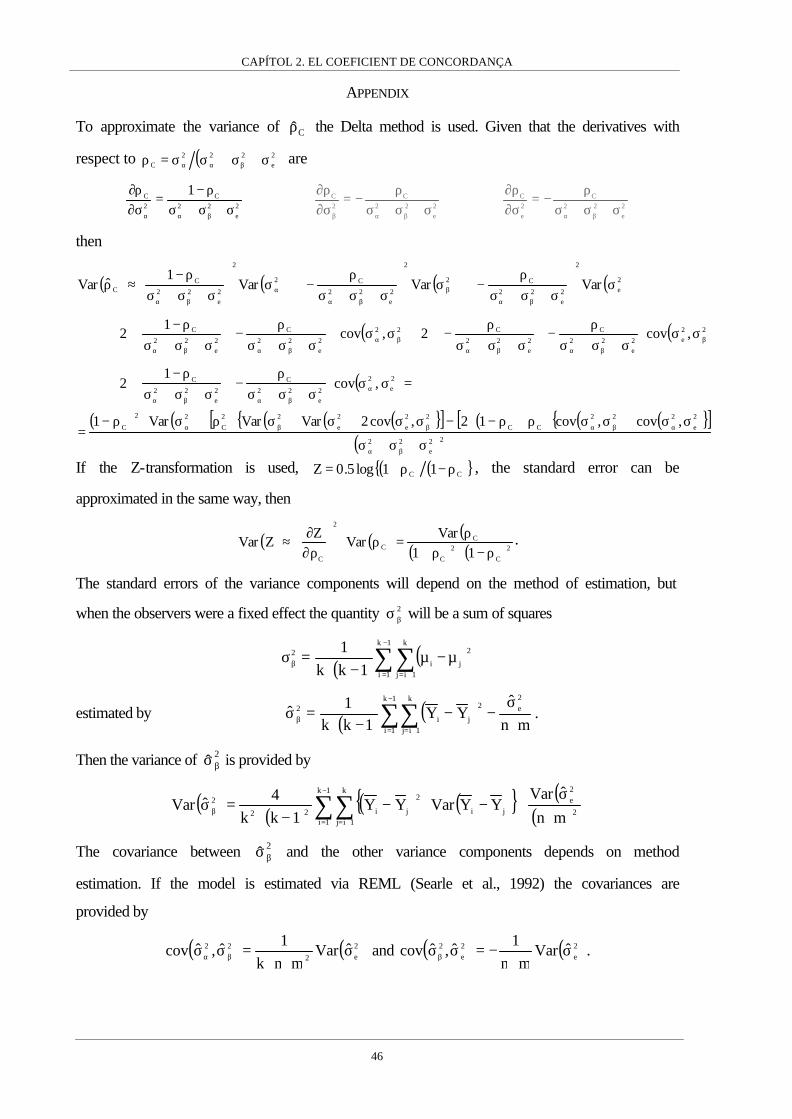
CAPÍTOL 2. EL COEFICIENT DE CONCORDANÇA
46
APPENDIX
To approximate the variance of Cρ the Delta method is used. Given that the derivatives with
respect to ( )2e
222C σ+σ+σσ=ρ βαα are
2e
22C
2C 1
σ+σ+σρ−
=σ∂ρ∂
βαα
2e
22C
2C
σ+σ+σρ
−=σ∂ρ∂
βαβ
2e
22C
2e
C
σ+σ+σρ
−=σ∂ρ∂
βα
then
( ) ( ) ( ) ( )
( ) ( )
( )
( ) ( ) ( ) ( ) ( ){ }[ ] ( ) ( ) ( ){ }[ ]( )22
e22
2
e
222
CC
22
e
2
e
22
C
22
C
2e
2
2e
22
C
2e
22
C
22e2
e22
C
2e
22
C22
2e
22
C
2e
22
C
2e
2
2e
22
C2
2
2e
22
C2
2
2e
22
CC
,cov,cov12,cov2VarVarVar1
,cov1
2
,cov2,cov1
2
VarVarVar1
ˆVar
σ+σ+σ
σσ+σσ⋅ρ⋅ρ−⋅−σσ+σ+σ⋅ρ+σ⋅ρ−=
=σσ
σ+σ+σρ
−
σ+σ+σρ−
⋅+
+σσ
σ+σ+σρ
−
σ+σ+σρ
−⋅+σσ⋅
σ+σ+σρ
−
σ+σ+σρ−
⋅+
+σ
σ+σ+σρ
−+σ
σ+σ+σρ
−+σ
σ+σ+σρ−
≈ρ
βα
αβαββα
α
βαβα
ββαβα
βαβαβα
βα
β
βα
α
βα
If the Z-transformation is used, ( ) ( ){ }CC 11log5.0Z ρ−ρ+= , the standard error can be
approximated in the same way, then
( ) ( ) ( )( ) ( )2
C
2
C
CC
2
C 11Var
VarZ
ZVarρ−⋅ρ+
ρ=ρ⋅
ρ∂
∂≈ .
The standard errors of the variance components will depend on the method of estimation, but
when the observers were a fixed effect the quantity 2βσ will be a sum of squares
( ) ( )∑∑−
= +=β µ−µ
−⋅=σ
1k
1i
k
1ij
2
ji2
1kk1
estimated by ( ) ( )mn
ˆYY
1kk1ˆ
2e
1k
1i
k
1ij
2
ji2
⋅σ
−−−⋅
=σ ∑∑−
= +=β .
Then the variance of 2ˆ βσ is provided by
( ) ( ) ( ) ( ){ } ( )( )2
2e
1k
1i
k
1ijji
2
ji22
2
mn
ˆVarYYVarYY
1kk4ˆVar
⋅σ
+−⋅−−⋅
=σ ∑∑−
= +=β
The covariance between 2ˆ βσ and the other variance components depends on method
estimation. If the model is estimated via REML (Searle et al., 1992) the covariances are
provided by
( ) ( )2e2
22 ˆVarmnk
1ˆ,ˆcov σ⋅⋅
=σσ βα and ( ) ( )2e
2e
2 ˆVarmn
1ˆ,ˆcov σ⋅
−=σσβ .

CAPÍTOL 2. EL COEFICIENT DE CONCORDANÇA
47
Estimació del Coeficient de Concordança amb dades de recompte
Introducció
Els procediments utilitzats per mesurar la concordança entre mètodes de mesura (observadors,
instruments de mesura, etc.) que mesuren en una escala quantitativa sovint assumeixen que el
model de mesura subjacent que genera les dades és lineal, amb efectes additius i amb les
dades distribuïdes sota lleis normals. Així el coeficient de correlació intraclasse o el coeficient
de variació intra-individu assumeixen el següent model de mesura (Fleiss, 1986)
ijjiij eY +β+α+µ=
on Yij és la dada corresponent a l’individu i-éssim mesurat amb el mètode j-éssim amb
i=1,...,n, j=1,...,k; αi és l’efecte aleatori individu amb ( )ασα ,0N~i ; β j és l’efecte del mètode
de mesura, que tant pot ser fix com aleatori depenent del disseny de les dades; finalment eij és
l’error aleatori que es distribueix sota una normal ( )eij ,0N~e σ .
Sota aquest model el coeficient de correlació intraclasse es defineix com el quocient entre la
covariança entre les dades d’un mateix cluster o classe respecte la variança marginal de les
dades
( )( ) 2
e22
2
ij
ilij
YVarY,Ycov
σ+σ+σσ
==ρβα
α
On 2βσ serà una variança si l’efecte mètode és aleatori, o una suma de quadrats
∑=
β β−
=σk
1j
2j
2
1k1
si és fix (Shrout and Fleiss, 1979; Rousson et al, 2002). En aquest darrer cas
s’ha demostrat (Carrasco and Jover, 2003) que el coeficient de correlació intraclasse que
s’obté és l’anomenat coeficient de concordança (Lin, 1989).
Una altra mesura utilitzada per avaluar la concordança entre mètodes de mesura és el
coeficient de variació intra-individu, que es defineix com
µ
σ+σ= β
2e
2
WCV .
Sota aquest model de mesura, el coeficient de correlació intraclasse és depenent de la
variabilitat entre individus (covariància entre observadors), mentre que el coeficient de
variació intra-individu és independent de la variabilitat entre individus però és depenent de la
mitjana.
CAPÍTOL 2. EL COEFICIENT DE CONCORDANÇA
48
La consistència de les estimacions dels components de la variància està subjecta al
compliment de les assumpcions de linealitat i normalitat dels efectes i de la homocedasticitat
de la variància de l’error, sobretot si s’utilitzen mètodes d’estimació basats en la
versemblança de les dades, com ara la màxima versemblança (ML) o la màxima
versemblança restringida (REML). Quan aquestes assumpcions no es compleixen els
investigadors opten per transformar les dades (Cunningham et al., 1997) o per utilitzar
procediments robustos d’estimació de les variàncies (Padmanabhan et al, 1997; King and
Chinchilli, 2001).
Aquesta situació és força habitual quan es treballa amb recomptes sense límit superior com
ara són els recomptes de cèl·lules, on les transformacions logaritme i arrel quadrada intenten
normalitzar les dades. En principi, el desavantatge més notable de transformar les dades és el
fet de no treballar amb l’escala original, però tant el coeficient de correlació intraclasse com el
coeficient de variació intra-individu són adimensionals i no es veuen afectats per canvis
d’escala. Per tant transformar sembla una bona solució, però sempre tenint en compte que
s’està ignorant el veritable procés de generació de les dades. D’altre banda el fet d’utilitzar
mesures robustes acostuma a comportar l’eliminació o variació de dades, un procediment
molt discutible si les dades extremes representen part del rang real de la variabilitat present en
la població d’individus en estudi.
Una hipòtesi de treball que sembla plausible en recomptes es considerar que la generació de
les dades es produeix sota el següent model de mesura:
( )ijiij Poisson~|Y µα , ( )ασα ,0N~i i ( ) jiijlog β+α+µ=µ .
Té sentit pensar que si aquest model és cert, l’estimació de les mesures de concordança
derivades de l’estimació de les components d’aquest model seran més consistents que
aquelles obtingudes mitjançant transformacions de les dades o procediments robustos.
L’objectiu d’aquest treball és definir aquestes mesures de concordança en el cas de que el
procés generador de les dades sigui una mixtura de Poisson i Normal, i estudiar el
comportament dels estimadors del coeficient de correlació intraclasse.
Mesures de concordança
Coeficient de correlació intraclasse
Com ha estat mencionat abans, el coeficient de correlació intraclasse (CCI) es defineix com el
quocient entre la covariança de les mesures d’una mateix classe o cluster i la variança
marginal de les dades. Per tant la correlació entre dues mesures preses a un mateix individu i
és

CAPÍTOL 2. EL COEFICIENT DE CONCORDANÇA
49
( )( )ij
ilij
YVarY,Ycov
=ρ
amb lj ≠ .
La covariança i les variances que apareixen en l’expressió del CCI es refereixen a la
distribució marginal de les dades, per tant es necessari definir-les.
Si Yi és el vector de dades d’un individu l’esperança ve donada per
( ) [ ][ ] [ ] ( )[ ]jiijiii expEE|yEEYE β+α+µ=µ=α=
Tot i que la majoria de les vegades l’efecte mètode serà formalment un efecte fix i per tant no
se’l considerarà un component de la variància, per definir un CCI que mesuri concordança
entre instruments és convenient tenir en compte la variabilitat entre instruments i considerar-
lo com un efecte aleatori, ( )βσβ ,0N~j , independentment de com sigui considerat en el
procés d’estimació (Carrasco and Jover, 2003). Així, assumint que els efectes individu i
instrument són independents i distribuïts normalment s’arriba a (McCulloch and Searle, 2001)
( ) ( ) ( )[ ] ( ) ( )
σ+σ+µ=β+αµ=β+αµ= βα
2expMexpexpEexpYE
22
jiujii
on Mu és la funció generatriu de moments.
L’expressió de la variança ve donada per
( ) [ ]( ) ( )[ ] ( ) ( ) [ ] [ ]( ){ }11eYEYEEVar|YVarE|YEVarYVar22
iiiiiiiii +−⋅==µ+µ=α+α= βα σ+σK
i la covariança per
( ) [ ] ( )1eYEY,Ycov22
iilij −⋅= ασ .
D’aquesta manera l’expressió del coeficient de correlació intraclasse, quan s’assumeix que la
distribució de les dades condicionada als individus és Poisson, que l’efecte individu es
distribueix sota una Normal i que la funció d’enllaç entre la mitjana i les covariables és el
logaritme, és
( )( )
[ ] ( )[ ] [ ]( ){ }
[ ] ( )[ ] ( ) 11eYE
1eYE
11eYEYE
1eYEYVar
Y,Ycov22
2
22
2
i
i
ii
2
i
i
ilij
+−⋅
−⋅=
+−⋅
−==ρ
βα
α
βα
α
σ+σ
σ
σ+σ
σ
Per tant, el coeficient de correlació intraclasse és funció de la variabilitat entre individus, de la
variabilitat entre mètodes i de la mitjana de les dades, essent aquests els components de la
variància en aquest model.
Cal fer esment de que encara que es transformin les dades i s’utilitzi l’expressió per dades
normals, la dependència sobre la mitjana continuarà estant implícita, donat que aquesta
CAPÍTOL 2. EL COEFICIENT DE CONCORDANÇA
50
dependència prové de la relació que hi ha entre la covariància i variància de les dades
originals amb la mitjana.
A més a més, el fet de que el coeficient de correlació intraclasse depengui de la mitjana
implica que la introducció de qualsevol variable confusora en el model modificarà la mitjana i
per tant actuarà com una interacció respecte el CCI, és a dir, s’obtindrà un CCI diferent per a
cada patró de covariables. Aquest fet és ignorat quan es realitza l’anàlisi sota un model
normal, bé amb la variable original o bé transformant-la.
Coeficient de variació intraindividu
El coeficient de variació intra-individu es defineix com el quocient de la variabilitat intra-
individu expressada com a desviació estàndard respecte la mitjana global de les dades.
Aquesta variabilitat en el model que s’està assumint és heterocedàstica donat que depèn de la
mitjana de cada individu, és a dir,
( ) [ ] ( )
σ+α+µ=β+α+µ=α=α β
2expexp|yE|yVar
2
ijiiiii
L’expressió del coeficient de variació intra-individu és
( )( )
( )
σ+α−σ+µ−=
σ+σ+µ
σ+
α+µ
=α
= β
α
βα
β
221
exp
2exp
42exp
yE|yVar
WCV2
i2
22
2
i
i
ii
Com es pot observar el WCV variarà d’individu a individu, fet totalment esperable si es té en
compte que el model es heteroscedastic per definició. A més a més, el WCV no tan sols és
depenent de la mitjana sinó que també depèn de la variabilitat entre individus, per tant la seva
principal virtut en el model normal és perd sota el present model. A l’igual que en el cas del
CCI aquesta dependència continuarà manifestant-se encara que es transformin les dades.
No obstant, aquesta mesura continua essent útil com a diagnòstic de la concordança, i pot
servir per avaluar quins individus són els que concorden més o menys i detectar possibles
outliers.
Per salvar el problema de tenir un WCV per a cada individu es podria considerar el WCV en
la mitjana de l’efecte individu, ( ) 0E i =α , aleshores
σ+σ+µ−= β
α 221
expAWCV2
2

CAPÍTOL 2. EL COEFICIENT DE CONCORDANÇA
51
Cal destacar que si en lloc d’utilitzar el coeficient de variació intra-individu es fa servir
l’índex d’agregació, les mesures que s’obtenen són
( )( )
σ
−α=
σ+σ+µ
σ+α+µ
=α
= α
βα
β
2exp
2exp
2exp
yE|yVar
AI2
i22
2
i
i
ii
i
σ−= α
2expAAI
2
mesura que tan sols depèn de la variabilitat entre individus.
Estimació
Sigui ( )u|Yf la funció de densitat de les dades condicionada als efectes aleatoris, i ( )uf la
funció de densitat dels efectes aleatoris. La versemblança de les dades ve donada per
( ) ( )∫= duufu|YfL
En el cas dels models mixtes normals s’assumeix que tant ( )u|Yf com ( )uf es distribueixen
sota distribucions Normals, i la funció d’enllaç entre la mitjana de la variable resposta i les
variables explicatives és la identitat. Aleshores la integral es pot resoldre i L té un forma
tancada que es pot maximitzar, concretament
( ) ( ) Vlog21
YVY21
Llog 1 −µ−′µ−−∝ −
on Y és el vector de respostes, µ és el vector de mitjanes que inclou els efectes fixes, V és la
matriu de variàncies i covàriancies de les dades
RZZDV +′=
essent Z la matriu de disseny dels efectes aleatoris, D la matriu de variàncies i covariàncies
dels efectes aleatoris i R la matriu de variàncies dels residuals.
La dificultat en la maximització de L (o logL) depèn de l’estructura dels efectes aleatoris, així
en el cas d’un únic efecte aleatori l’expressió dels estimadors dels efectes fixes i dels
components de la variància es pot derivar analíticament (Searle et al. 1992), però amb
estructures més complicades l’estimació per màxima versemblança s’ha de dur a terme amb
mètodes iteratius com l’algoritme Fisher-Scoring.
Una alternativa a l’estimació dels components de la variància per màxima versemblança és la
màxima versemblança restringida (REML), la qual maximitza la versemblança de
combinacions lineals de Y de forma que la versemblança resultant no inclou els efectes fixes.
D’aquesta manera l’estimació dels components de la variància es duu a terme amb

CAPÍTOL 2. EL COEFICIENT DE CONCORDANÇA
52
independència de l’estimació dels efectes fixes i tenint en compte la pèrdua de graus de
llibertat, resultant estimadors no esbiaixats dels components de la variància.
Els models mixtes lineals generalizats (GLMM) permeten que tant la distribució ( )α|Yf
com ( )αf siguin qualsevol de la família exponencial, així com que la funció d’enllaç entre la
mitjana i les variables explicatives sigui no lineal. Per tant, el model mixt normal és un cas
particular dels models mixtes generalitzats.
La primera dificultat dels GLMM es resoldre la integral per trobar l’expressió de la
versemblança. Aquesta integral sovint és difícil de resoldre, sobretot amb estructures
complicades dels efectes aleatoris. En el cas d’un sol efecte aleatori, la integral es pot
aproximar pel mètode de la quadratura Gauss-Hermite i maximitzar la versemblança resultant.
Aquest mètode també funciona per dos efectes aleatoris aniuats, però no per dos efectes
creuats o més efectes aniuats (McCulloch and Searle, 2001). Entre les alternatives d’estimació
que han estat considerades es pot trobar els algoritmes Markov Chain Monte Carlo (Robert
and Casella, 1999) basats en estimació bayesiana, o d’altres fonamentats en simular la
versemblança (Mc Culloch, 1997).
Breslow and Clayton (1993) van proposar que la funció de densitat de les dades condicionada
als efectes aleatoris, ( )u|Yf , fos la quasi-versemblança (McCullagh and Nelder, 1989), i que
( )uf fos una Normal. Aleshores van resoldre la integral per trobar la versemblança mitjançant
el mètode d’aproximacions de Laplace, resultant una log-versemblança proporcional a
( ) uDu21
u|YflogPQL 1−′−=
on el logaritme de la quasi-versemblaça es veu “penalitzat” per un terme depenent dels efectes
aleatoris. Aquest fet va fer que aquest mètode d’estimació s’anomenés penalized quasi-
likelihood (PQL). Els efectes fixes i aleatoris (u) són estimats maximitzant PQL, mentre que
els components de la variància s’estimen mitjançant la REML dels efectes aleatoris. El procés
d’estimació és iteratiu on tant els efectes fixes i aleatoris com els components de la variància
es van actualitzant fins aconseguir la convergència de les estimacions a una solució.
El mètode PQL s’ha popularitzat força perquè al treballar amb la quasi-versemblança tan sols
s’ha de definir la relació entre la mitjana i la variància de les dades condicionades als efectes
aleatoris, així com la funció d’enllaç entre la mitjana i les covariables. No obstant, s’ha
demostrat (Breslow and Lin, 1995; Lin and Breslow, 1996) que les estimacions PQL són
força esbiaixades si la distribució real de les dades condicionades als efectes aleatoris
s’allunya de la Normal, com en el cas de la Binomial. Tot i això, si la distribució és Poisson
amb una mitjana de 7 o superior el mètode funciona correctament.

CAPÍTOL 2. EL COEFICIENT DE CONCORDANÇA
53
Error estàndard
En aquest apartat s’exposarà l’expressió de l’error estàndard del CCI si és estimat amb el
model mixt generalitzat Poisson-Normal. L’expressió de l’error estàndard així com d’altres
aspectes inferencials referents al CCI pel cas Normal-Normal es poden trobar a Carrasco i
Jover (2003).
Donat que el CCI en el model Poisson-Normal és funció de la mitjana, la variància entre
individus i la variabilitat dels mètodes, el seu error estàndard també serà funció de l’error
estàndard d’aquests paràmetres. Aquest s’aproxima mitjançant el mètode delta
( ) ( ) ( ) ( ) ( )
( ) ( )22
22
2
2
2
2
2
2
2
2
2
2
2
ˆ,ˆcov2ˆ,ˆcov2
ˆ,ˆcov2ˆVarˆVarˆVarˆVar
βαβα
ββ
α
α
β
α
α
α
σσ
δσδρ
δσδρ
+σµ
δσδρ
δµδρ
+
+σµ
δσδρ
δµδρ
+σ
δσδρ
+σ
δσδρ
+µ
δµδρ
≈ρ
Les expressions de les variàncies i covariàncies dependran del mètode d’estimació, sobretot
de com es dugui a terme l’estimació de l’efecte observador. Així, si tenim dos observadors i
aquest efecte es considera fix, els paràmetres d’interès a estimar serien µ (intercept), 1β
(efecte mètode) i 2ασ (variància entre individus). Aleshores, sota l’assumpció de que els
components de la variància i els efectes fixes no covarien (Searle et al, 1992) es pot assumir
que la única covariància diferent de 0 és
( ) ( ) ( )1121
21
2 ˆ,ˆcovˆˆ,ˆcov21ˆ
21
,ˆcovˆ,ˆcov βµ⋅β≈βµ=
βµ=σµ β
En canvi, si l’efecte observador és aleatori distribuït sota una Normal de variància 2βσ , l’única
covariància diferent de 0 serà ( )22 ˆ,ˆcov βα σσ .
Les variàncies i covariàncies de les estimacions dels components de la variància
s’aproximaran mitjançant la inversa de la matriu d’informació de Fisher.
Aquí ens centrarem en la situació de dos observadors i l’efecte mètode fix, aleshores
( ) ( ) ( ) ( ) ( )2
2
2
2
2
2
2
2
2
ˆ,ˆcov2ˆVarˆVarˆVarˆVar β
β
β
α
α
α
σµ
δσδρ
δµδρ
+σ
δσδρ
+σ
δσδρ
+µ
δµδρ
≈ρ
CAPÍTOL 2. EL COEFICIENT DE CONCORDANÇA
54
Derivades
( )( )
−σ
−σ+σρ−ρ=
µ∂ρ∂
α
βα
1exp
1exp1
2
22
; ( )[ ] ( ) ( )( ){ }[ ]1exp31exp31exp2
22222
−σ+σρ−−σ−σ
ρ=
σ∂ρ∂
βαα
αα
;
( )[ ] ( ) ( )( ){ }[ ]1exp31exp1exp2
222
22−σ+σρ−−σ
−σρ
=σ∂ρ∂
βαααβ
Estimació per interval
L’estimació per interval del coeficient de correlació intraclasse es durà a terme utilitzant la
transformació Z de Fisher,
( ) ( ) ( ){ }CCC1
C 11ln5.0tanhZ ρ−ρ+⋅=ρ= −
Aquesta transformació s’ha utilitzat amb èxit pel casos del coeficient de correlació de Pearson
i el coeficient de correlació intraclasse amb el model mixt Normal, distribuint-se ZC sota una
Normal.
Pel cas del model Poisson-Normal aquesta transformació també hauria de funcionar si les
estimacions són consistents. Així, un altre objectiu d’aquest treball serà comprovar si el
procediment de la transformació Z és útil en aquest cas.
Exemples
Es desitja avaluar la concordança entre quatre mètodes de recomptes de CD4, que
anomenarem A, B, C i D, els quals són comparats dos a dos. La concordança entre els
mètodes es valora mitjançant el coeficient de correlació intraclasse, que és estimat mitjançant
un model mixt normal utilitzant com a resposta la variable original i transformada,
considerant les transformacions logarítmiques i arrel quadrada. També s’estima el CCI
mitjançant un model mixt generalitzat assumint que els efectes mixtes es distribueixen sota
una normal i que la distribució de la variabilitat intra-individu és Poisson, utilitzant com a
procediment d’estimació el penalized quasi-likelihood. Per estimar els models mixtes normals
s’ha utilitzat la funció lme del programa S-Plus v.6.1 (Venables and Ripley, 1999) i per fer les
estimacions PQL s’ha utilitzat la funció glmm.PQL que es troba dins de la llibreria MASS
disponible a http://www.stats.ox.ac.uk/pub/MASS4/.
Per la comparació entre els mètodes es donen els gràfics de residus, les estimacions puntuals i
l’error estàndard del CCI.
Dels resultats (Apèndix I) es pot derivar que, en general, l’estimació del coeficient de
correlació intraclasse amb el model mixt generalizat tendeix a donar valors superiors que la
resta de mètodes, tret de la comparació B-C on les estimacions són similars. Donat que el

CAPÍTOL 2. EL COEFICIENT DE CONCORDANÇA
55
valor real del CCI és desconegut no es pot concloure si els models mixtes normals
l’infraestimen o si el GLMM el sobreestima.
Pel que fa al comportament dels residuals, els derivats del GLMM sempre tenen un
comportament similar o millor que la resta. D’altre banda, l’error estàndard estimat per
GLMM és sistemàticament inferior.
Simulació
Amb l’objectiu d’analitzar el comportament de l’estimació del coeficient de correlació
intraclasse quan és estimat utilitzant models lineals mixtes (normal-normal) i models lineals
mixtes generalitzats (normal-poisson), es duu a terme un estudi de simulació on dos
observadors són comparats. Les dades seran generades mitjançant una mixtura de Poisson per
la variabilitat intra-individu i de Normal per l’efecte individu, utilitzant el logaritme com
funció d’enllaç entre la mitjana i els efectes. L’efecte observador es considera fix.
Les situacions que es generaran es representen a la Taula 7. Aquestes combinen diferents
valors de mitjanes, variància entre individus i variabilitat entre mètodes. Es consideren mides
mostrals de 30 i 100 individus. Per a cada combinació es generaran 1000 mostres i el CCI serà
estimat mitjançant un model mixt normal amb la variable original, transformada
logarítmicament i per l’arrel quadrada, i amb un GLMM amb una mixtura Poisson-Normal
estimat per PQL.
El comportament de les estimacions s’ha avaluat tant en termes de biaix com de precisió. El
biaix s’ha estimat com a diferència entre la mitjana de les estimacions i el valor real simulat,
mentre que la precisió s’ha valorat calculant la desviació típica de les estimacions. Amb
l’objectiu d’avaluar si l’error estàndard és estimat correctament s’ha comparat la desviació
típica de les estimacions amb la mitjana dels errors estàndards, calculada aquesta com l’arrel
quadrada de la mitjana de les variàncies estimades. La consistència de les estimacions s’ha
avaluat mitjançant l’error quadràtic mig, el qual es troba composat pel biaix al quadrat més la
variància de les estimacions. Aquests resultats es mostren a la Taula 8.
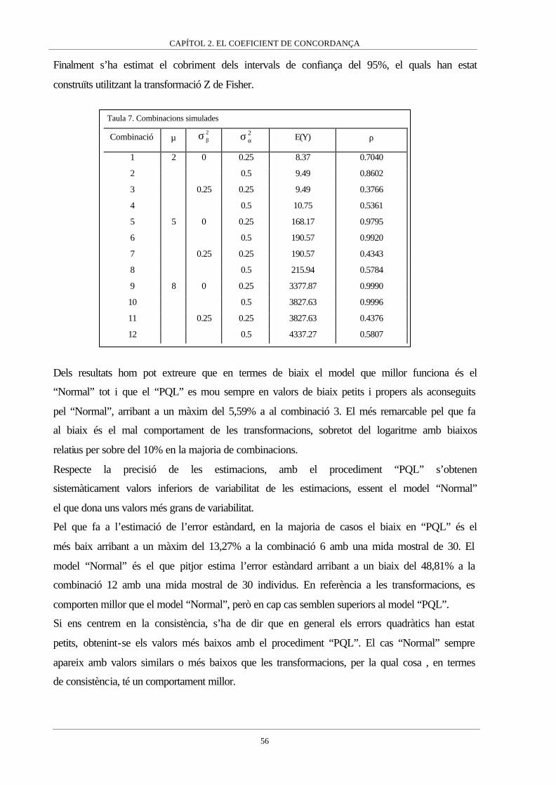
CAPÍTOL 2. EL COEFICIENT DE CONCORDANÇA
56
Finalment s’ha estimat el cobriment dels intervals de confiança del 95%, el quals han estat
construïts utilitzant la transformació Z de Fisher.
Dels resultats hom pot extreure que en termes de biaix el model que millor funciona és el
“Normal” tot i que el “PQL” es mou sempre en valors de biaix petits i propers als aconseguits
pel “Normal”, arribant a un màxim del 5,59% a al combinació 3. El més remarcable pel que fa
al biaix és el mal comportament de les transformacions, sobretot del logaritme amb biaixos
relatius per sobre del 10% en la majoria de combinacions.
Respecte la precisió de les estimacions, amb el procediment “PQL” s’obtenen
sistemàticament valors inferiors de variabilitat de les estimacions, essent el model “Normal”
el que dona uns valors més grans de variabilitat.
Pel que fa a l’estimació de l’error estàndard, en la majoria de casos el biaix en “PQL” és el
més baix arribant a un màxim del 13,27% a la combinació 6 amb una mida mostral de 30. El
model “Normal” és el que pitjor estima l’error estàndard arribant a un biaix del 48,81% a la
combinació 12 amb una mida mostral de 30 individus. En referència a les transformacions, es
comporten millor que el model “Normal”, però en cap cas semblen superiors al model “PQL”.
Si ens centrem en la consistència, s’ha de dir que en general els errors quadràtics han estat
petits, obtenint-se els valors més baixos amb el procediment “PQL”. El cas “Normal” sempre
apareix amb valors similars o més baixos que les transformacions, per la qual cosa , en termes
de consistència, té un comportament millor.
Taula 7. Combinacions simulades
Combinació µ 2βσ 2
ασ E(Y) ρ
1 2 0 0.25 8.37 0.7040
2 0.5 9.49 0.8602
3 0.25 0.25 9.49 0.3766
4 0.5 10.75 0.5361
5 5 0 0.25 168.17 0.9795
6 0.5 190.57 0.9920
7 0.25 0.25 190.57 0.4343
8 0.5 215.94 0.5784
9 8 0 0.25 3377.87 0.9990
10 0.5 3827.63 0.9996
11 0.25 0.25 3827.63 0.4376
12 0.5 4337.27 0.5807

CAPÍTOL 2. EL COEFICIENT DE CONCORDANÇA
57
Respecte els cobriments, el procediment “Normal” tan sols dona uns cobriments correctes en
les combinacions 3 i 4, sobreestimant el cobriment nominal en les combinacions 7,8,11 i 12.
També es posa de manifest que els cobriments en els procediments que impliquen
transformacions són força dolents, sobretot en el cas del logaritme que en alguns casos no
arriba a un cobriment del 10%. Pel que fa al procediment “PQL” els cobriments són molt
correctes en tots els casos, trobant-se que la transformació Z no millora els cobriments en
general.
També s’ha estudiat l’aproximació a la distribució Normal de les estimacions del CCI quan
aquest s’estima per PQL. En els casos en que s’utilitza un model normal ja ha estat comprovat
que el CCI es distribueix assimptòticament sota una Normal per mides mostrals grans, i que la
transformació Z millora considerablement l’aproximació (Carrasco and Jover, 2003). Però en
el cas del PQL el procés d’estimació no és del tot màxim versemblant, pel que sembla
interessant analitzar si aquesta aproximació a la Normal es manté. Amb aquesta finalitat s’han
construït gràfics quantile-quantile amb les estimacions realitzades de l’CCI amb PQL i de la
transformació Z d’aquestes estimacions (Apèndix II). Amb l’ajut d’aquests gràfics es pot
observar que l’aproximació assimptòtica a la Normal del CCI és molt bona en les
combinacions en que hi ha variabilitat entre mètodes i amb una mida mostral de 100. Quan
s’aplica la transformació Z l’aproximació millora considerablement fins i tot amb una mida
mostral de 30.
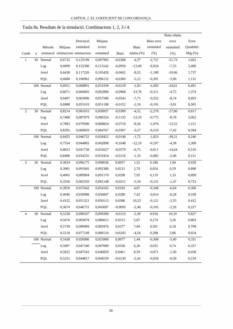
CAPÍTOL 2. EL COEFICIENT DE CONCORDANÇA
58
Taula 8a. Resultats de la simulació. Combinacions 1, 2, 3 i 4.
Comb n
Mètode
estimació
Mitjana
estimacions
Desviació
estàndard
estimacions
Mitjana
errors
estàndard Biaix
Biaix
relatiu (%)
Biaix error
estàndard
(%)
Biaix relatiu
error
estàndard
(%)
Error
Quadràtic
Mig (%)
1 30 Normal 0,6732 0,125198 0,097992 -0,0308 -4,37 -2,721 -21,73 1,662
Log 0,6090 0,122380 0,113142 -0,0950 -13,49 -0,924 -7,55 2,400
Arrel 0,6438 0,117226 0,105428 -0,0602 -8,55 -1,180 -10,06 1,737
PQL 0,6680 0,100062 0,096155 -0,0360 -5,12 -0,391 -3,90 1,131
100 Normal 0,6911 0,068891 0,051939 -0,0129 -1,83 -1,695 -24,61 0,491
Log 0,6071 0,066005 0,062890 -0,0968 -13,76 -0,311 -4,72 1,374
Arrel 0,6497 0,063096 0,057580 -0,0543 -7,71 -0,552 -8,74 0,693
PQL 0,6888 0,053103 0,051188 -0,0152 -2,16 -0,191 -3,61 0,305
2 30 Normal 0,8214 0,081633 0,058937 -0,0389 -4,52 -2,270 -27,80 0,817
Log 0,7468 0,087979 0,080254 -0,1135 -13,19 -0,773 -8,78 2,062
Arrel 0,7883 0,079580 0,068824 -0,0719 -8,36 -1,076 -13,52 1,151
PQL 0,8295 0,069959 0,064767 -0,0307 -3,57 -0,519 -7,42 0,584
100 Normal 0,8455 0,046752 0,028422 -0,0148 -1,72 -1,833 -39,21 0,240
Log 0,7554 0,044865 0,042898 -0,1048 -12,19 -0,197 -4,38 1,300
Arrel 0,8023 0,041738 0,035627 -0,0579 -6,73 -0,611 -14,64 0,510
PQL 0,8486 0,034235 0,033414 -0,0116 -1,35 -0,082 -2,40 0,131
3 30 Normal 0,3824 0,096175 0,098036 0,0057 1,52 0,186 1,94 0,928
Log 0,3981 0,091845 0,092386 0,0215 5,70 0,054 0,59 0,890
Arrel 0,4065 0,089984 0,091179 0,0298 7,92 0,119 1,33 0,899
PQL 0,3556 0,082359 0,081148 -0,0211 -5,59 -0,121 -1,47 0,723
100 Normal 0,3950 0,057642 0,054162 0,0183 4,87 -0,348 -6,04 0,366
Log 0,4046 0,050988 0,050847 0,0280 7,42 -0,014 -0,28 0,338
Arrel 0,4152 0,051321 0,050113 0,0386 10,25 -0,121 -2,35 0,412
PQL 0,3674 0,046751 0,045697 -0,0093 -2,46 -0,105 -2,26 0,227
4 30 Normal 0,5238 0,090107 0,099289 -0,0123 -2,30 0,918 10,19 0,827
Log 0,5676 0,083878 0,086615 0,0315 5,87 0,274 3,26 0,803
Arrel 0,5739 0,080969 0,085976 0,0377 7,04 0,501 6,18 0,798
PQL 0,5118 0,077149 0,080124 -0,0243 -4,54 0,298 3,86 0,654
100 Normal 0,5438 0,056986 0,053908 0,0077 1,44 -0,308 -5,40 0,331
Log 0,5697 0,047340 0,047689 0,0336 6,26 0,035 0,74 0,337
Arrel 0,5822 0,047543 0,046829 0,0461 8,59 -0,071 -1,50 0,438
PQL 0,5231 0,044817 0,044559 -0,0130 -2,42 -0,026 -0,58 0,218

CAPÍTOL 2. EL COEFICIENT DE CONCORDANÇA
59
Taula 8b. Resultats de la simulació. Combinacions 5, 6, 7 i 8.
Comb n
Mètode
estimació
Mitjana
estimacions
Desviació
estàndard
estimacions
Mitjana
errors
estàndard Biaix
Biaix
relatiu (%)
Biaix error
estàndard
(%)
Biaix relatiu
error
estàndard
(%)
Error
Quadràtic
Mig (%)
5 30 Normal 0,9762 0,010988 0,008696 -0,0033 -0,33 -0,229 -20,86 0,013
Log 0,9685 0,011853 0,011487 -0,0110 -1,13 -0,037 -3,08 0,026
Arrel 0,9739 0,010538 0,009549 -0,0056 -0,57 -0,099 -9,39 0,014
PQL 0,9758 0,008950 0,007958 -0,0037 -0,37 -0,099 -11,07 0,009
100 Normal 0,9779 0,005723 0,004389 -0,0016 -0,16 -0,133 -23,31 0,004
Log 0,9696 0,006074 0,006009 -0,0099 -1,01 -0,006 -1,06 0,013
Arrel 0,9751 0,005242 0,004939 -0,0044 -0,45 -0,030 -5,80 0,005
PQL 0,9784 0,004114 0,003946 -0,0011 -0,11 -0,017 -4,09 0,002
6 30 Normal 0,9896 0,005538 0,003849 -0,0024 -0,24 -0,169 -30,50 0,004
Log 0,9822 0,007269 0,006532 -0,0098 -0,98 -0,074 -10,14 0,015
Arrel 0,9876 0,005414 0,004563 -0,0044 -0,44 -0,085 -15,71 0,005
PQL 0,9901 0,004516 0,003916 -0,0019 -0,19 -0,060 -13,27 0,002
100 Normal 0,9909 0,002952 0,001826 -0,0011 -0,11 -0,113 -38,14 0,001
Log 0,9827 0,003537 0,003439 -0,0092 -0,93 -0,010 -2,76 0,010
Arrel 0,9884 0,002579 0,002308 -0,0035 -0,36 -0,027 -10,52 0,002
PQL 0,9915 0,002016 0,001915 -0,0005 -0,05 -0,010 -5,03 <0,001
7 30 Normal 0,4379 0,065559 0,084334 0,0036 0,82 1,878 28,64 0,431
Log 0,4879 0,067050 0,066582 0,0536 12,33 -0,047 -0,70 0,736
Arrel 0,4761 0,066333 0,071440 0,0418 9,63 0,511 7,70 0,615
PQL 0,4207 0,058872 0,057175 -0,0136 -3,14 -0,170 -2,88 0,365
100 Normal 0,4481 0,040819 0,046567 0,0138 3,17 0,575 14,08 0,186
Log 0,4927 0,036335 0,036518 0,0584 13,45 0,018 0,50 0,473
Arrel 0,4822 0,037861 0,039219 0,0479 11,02 0,136 3,59 0,373
PQL 0,4301 0,032108 0,031799 -0,0043 -0,98 -0,031 -0,96 0,105
8 30 Normal 0,5702 0,061130 0,089008 -0,0081 -1,41 2,788 45,60 0,380
Log 0,6539 0,061874 0,060189 0,0755 13,05 -0,169 -2,72 0,953
Arrel 0,6342 0,061550 0,068633 0,0558 9,65 0,708 11,51 0,690
PQL 0,5649 0,053856 0,051094 -0,0135 -2,33 -0,276 -5,13 0,308
100 Normal 0,5847 0,039287 0,048694 0,0063 1,09 0,941 23,95 0,158
Log 0,6588 0,032291 0,032772 0,0804 13,90 0,048 1,49 0,751
Arrel 0,6417 0,035041 0,037363 0,0633 10,94 0,232 6,63 0,523
PQL 0,5738 0,028004 0,027961 -0,0046 -0,79 -0,004 -0,15 0,081

CAPÍTOL 2. EL COEFICIENT DE CONCORDANÇA
60
Taula 8c. Resultats de la simulació. Combinacions 9, 10, 11 i 12.
Comb n
Mètode
estimació
Mitjana
estimacions
SD
estimacions
Mitjana
errors
estàndard Biaix
Biaix
relatiu
(%)
Biaix error
estàndard
(%)
Biaix relatiu
error
estàndard
(%)
Error
Quadràtic
Mig (%)
9 30 Normal 0,9988 0,000537 0,000458 -0,0002 -0,02 -0,008 -14,70 <0,001
Log 0,9984 0,000569 0,000599 -0,0006 -0,06 0,003 5,27 <0,001
Arrel 0,9987 0,000505 0,000500 -0,0003 -0,03 0,000 -0,94 <0,001
PQL 0,9988 0,000460 0,000409 -0,0002 -0,02 -0,005 -11,11 <0,001
100 Normal 0,9989 0,000293 0,000224 -0,0001 -0,01 -0,007 -23,60 <0,001
Log 0,9984 0,000292 0,000312 -0,0005 -0,05 0,002 6,82 <0,001
Arrel 0,9987 0,000257 0,000254 -0,0002 -0,02 0,000 -1,06 <0,001
PQL 0,9989 0,000211 0,000201 -0,0001 -0,01 -0,001 -4,70 <0,001
10 30 Normal 0,9995 0,000279 0,000200 -0,0001 -0,01 -0,008 -28,18 <0,001
Log 0,9991 0,000327 0,000334 -0,0005 -0,05 0,001 2,04 <0,001
Arrel 0,9994 0,000256 0,000234 -0,0002 -0,02 -0,002 -8,63 <0,001
PQL 0,9995 0,000224 0,000197 -0,0001 -0,01 -0,003 -11,96 <0,001
100 Normal 0,9995 0,000161 0,000094 -0,0001 -0,01 -0,007 -41,90 <0,001
Log 0,9991 0,000182 0,000178 -0,0005 -0,05 0,000 -2,22 <0,001
Arrel 0,9994 0,000137 0,000118 -0,0002 -0,02 -0,002 -13,41 <0,001
PQL 0,9996 0,000101 0,000096 0,0000 0,00 -0,001 -5,30 <0,001
11 30 Normal 0,4422 0,063691 0,083540 0,0046 1,04 1,985 31,16 0,408
Log 0,4949 0,068073 0,064538 0,0572 13,07 -0,354 -5,19 0,791
Arrel 0,4815 0,066190 0,070126 0,0438 10,01 0,394 5,95 0,630
PQL 0,4260 0,059000 0,054978 -0,0116 -2,65 -0,402 -6,82 0,362
100 Normal 0,4516 0,039213 0,046091 0,0139 3,19 0,688 17,54 0,173
Log 0,4984 0,036008 0,035408 0,0608 13,89 -0,060 -1,67 0,499
Arrel 0,4864 0,037028 0,038485 0,0488 11,15 0,146 3,93 0,375
PQL 0,4343 0,031203 0,030547 -0,0034 -0,77 -0,066 -2,10 0,098
12 30 Normal 0,5728 0,059431 0,088439 -0,0078 -1,35 2,901 48,81 0,359
Log 0,6591 0,061973 0,058074 0,0785 13,52 -0,390 -6,29 1,000
Arrel 0,6374 0,061138 0,067564 0,0568 9,78 0,643 10,51 0,696
PQL 0,5678 0,053070 0,048801 -0,0129 -2,22 -0,427 -8,04 0,298
100 Normal 0,5878 0,038702 0,048319 0,0071 1,23 0,962 24,85 0,155
Log 0,6644 0,032068 0,031591 0,0838 14,43 -0,048 -1,49 0,805
Arrel 0,6453 0,034760 0,036754 0,0646 11,13 0,199 5,73 0,538
PQL 0,5771 0,027280 0,026652 -0,0036 -0,62 -0,063 -2,30 0,076

CAPÍTOL 2. EL COEFICIENT DE CONCORDANÇA
61
Taula 9. Cobriments dels intervals de confiança
Normal Logaritme Arrel PQL
Comb n Asymp Z-trans Asymp Z-trans Asymp Z-trans Asymp Z-trans
1 30 88,0 86,7 93,3 85,5 93,5 87,9 94,1 93,0
100 85,9 84,7 69,8 61,0 88,5 81,2 95,0 92,6
2 30 86,3 80,2 85,6 61,3 92,2 78,2 93,8 90,4
100 77,3 72,8 23,4 15,4 68,6 54,9 94,9 92,6
3 30 94,4 95 92,4 94,5 93,5 96 91,1 91
100 93,2 93,7 90,6 91,9 88,2 88,7 92,0 91,5
4 30 95,7 95,7 90,3 94,2 90,5 94,7 93,7 93,2
100 94,7 94,1 87,4 90,2 80,0 83,6 94,3 93,1
5 30 90,5 90,7 97,9 84,4 97,1 91,4 95,1 91,9
100 89,8 86,6 73,9 53,2 93,2 84,7 95,5 94,5
6 30 87,5 81,2 90,6 51,5 97,8 82,3 95,2 90,8
100 81,1 76,0 11,3 3,9 73,8 57,9 94,3 93,6
7 30 98,1 97,9 86,5 90,3 91,7 93,7 92,1 91,8
100 96,2 97,0 64,3 68,1 78,1 81,1 94,0 93,7
8 30 99,2 99 71,4 78,6 87,1 91,5 93,2 92,4
100 96,6 98,5 32,7 38,7 60,1 67,1 93,6 94,1
9 30 92,3 89,1 98,8 86,5 97,1 92,3 95,8 91
100 87,9 85,7 73,9 51,3 94,4 86,4 94,6 94,1
10 30 89,2 79,6 94,2 47,9 98,3 81,7 95,4 91
100 76,4 71,0 9,1 2,9 73,7 58,2 94,4 94,0
11 30 98,4 98,5 82,9 87 91,2 94,1 91,8 91,6
100 96,4 97,4 59,4 62,7 77,9 81,2 93,9 93,9
12 30 99,3 99 67 74,2 87 91,5 92,6 92
100 96,8 98,6 27,2 30,7 57,6 64,3 94,0 93,6
Discussió
El coeficient de correlació intraclasse és una mesura àmpliament utilitzada per avaluar la
intercanviabilitat entre mètodes de mesura. Habitualment aquest s’estima mitjançant els
components de la variància d’un model lineal amb efectes mixtes assumint que tant els efectes
aleatoris com el residu es distribueixen sota distribucions normals. Però de vegades
l’assumpció de normalitat del residu no és possible per la pròpia naturalesa de les dades, com
és en el cas de que la variable que s’està mesurant consisteixi en recomptes sense límit

CAPÍTOL 2. EL COEFICIENT DE CONCORDANÇA
62
superior. Aquesta situació es dona, per exemple, quan es vol avaluar la concordança entre
analitzadors automàtics que proporcionen com a resultat recomptes de cèl·lules. Aleshores la
pràctica habitual és o bé assumir que el residual s’aproximarà a una Normal, o bé aplicar
transformacions a les dades que accelerin aquesta aproximació. Els models lineals mixtes
generalitzats permeten una nova solució, possibilitant que el residu tingui una distribució
pròpia d’un recompte com és la distribució de Poisson.
Com s’ha observat en l’estudi de simulació, en aquests casos el model mixt generalitzat
funciona millor en termes de consistència i cobriment dels intervals de confiança que els
procediments basats en el model lineal mixt clàssic. A més a més, s’ha observat que les
transformacions no funcionen gaire bé, fins i tot posant-se de relleu que dona millor resultat
treballar amb les dades originals que amb les transformacions. Aquest fet pot ser degut a que
les transformacions són útils quan es treballa amb dades amb valors extrem i/o
heterocedàstiques. Però la introducció d’un efecte individu pot explicar en gran part la
presencia de valors extrems. Si, a més a més, es permet que el residual pugui ser
heterocedastic, com en els GLMM, queda clar que aquestes transformacions resulten
innecessàries i fins i tot desaconsellables donat que, com s’ha vist a la simulació, les
estimacions que en resulten són força esbiaixades. Des d’aquesta perspectiva, seria preferible
l’ús d’un model lineal mixt clàssic amb les dades originals que transformades. No obstant, el
model mixt clàssic amb les dades originals s’ha presentat com poc eficient i amb els errors
estàndard mal estimats, qüestió que ha provocat uns cobriments pobres dels intervals de
confiança.
Pel que fa al mètode d’estimació, la tècnica penalized quasi-likelihood ha donat estimacions
correctes de les components de la variança i del coeficient de correlació intraclasse, tot i no
ser una tècnica completament “màxim-versemblant”. Recentment s’està treballant en el
desenvolupament de funcions que estimin aquests model per màxima-versemblança
aproximant l’integral involucrada en la versemblança mitjançant la quadratura Gauss-Hermite
(McCulloch and Searle, 2001) amb un únic efecte aleatori, com seria el cas del coeficient de
correlació intraclasse presentat aquí. Tot i que l’estimació PQL ha estat raonablement
correcta, desconeixem si utilitzant un procediment d’estimació basat completament en la
versemblança s’obtindran estimacions més consistents.
Referencies
Breslow, NE and Clayton DG (1993). “Approximate inference in generalized linear mixed
models”. Journal of tje American Statistical Association, 88:9-25.

CAPÍTOL 2. EL COEFICIENT DE CONCORDANÇA
63
Breslow, NE and Lin, X. (1995). “Bias correction in generalized linear mixed models with a
single component of dispersion”. Biometrika, 82:81-91.
Carrasco, JL and Jover, L. (2003). “Estimating the generalized concordance correlation
coefficient through variance components”. Biometrics. In press.
Cunningham, WE, Rana, HM, Shapiro, MF and Hays, RD (1997). “Reliability and validity of
self-report CD4 counts in persons hospitalized with HIV disease”. Journal of Clinical
Epidemiology, 50(7):829-835.
King, TS and Chinchilli, VM. (2001). “Robust estimators of the concordance correlation
coefficient”. Journal of the Biopharmaceutical Statistics, 11(3):83-105.
Lin, X and Breslow, NE (1996). “Bias correction in generalized linear mixed models with
multiple components of dispersion”. Journal of the American Statistical Association,
91:1007-1016.
McCullagh, P and Nelder, JA (1989). Generalized Linear Models, 2nd Ed. Chapman & Hall,
London.
Padmanabhan AR, Chinchilli VM, Babu GJ.(1997) “Robust analysis of within-unit variances
in repeated measurement experiments” Biometrics 53: 1520-1526.
Robert, CP and Casella G. (1999). Monte Carlo Statistical Methods. Springer-Velag, New
York.
McCulloch, CE. (1997). “Maximum likelihood algorithms for generalized linear mixed
models”. Journal of the American Statistical Association, 92:162-170.
McCulloch, CE and Searle, SR. (2001). Generalized, Linear and Mixed Moldels. John Wiley
& Sons, New York.
Rousson V, Gasser T, Seifert B. (2002) “Assessing intrarater, interrater and test-retest
reliability of continous measurements”. Statistics in Medicine 21:3431-3446
Searle, R.S., Casella, G. and McCulloch, C.E. (1992). Variance Components. New York:
Wiley.
Venables, W. N. and Ripley, B. D. (1999). Modern Applied Statistics with S-PLUS (3rd
Edition). New York: Springer-Verlag.
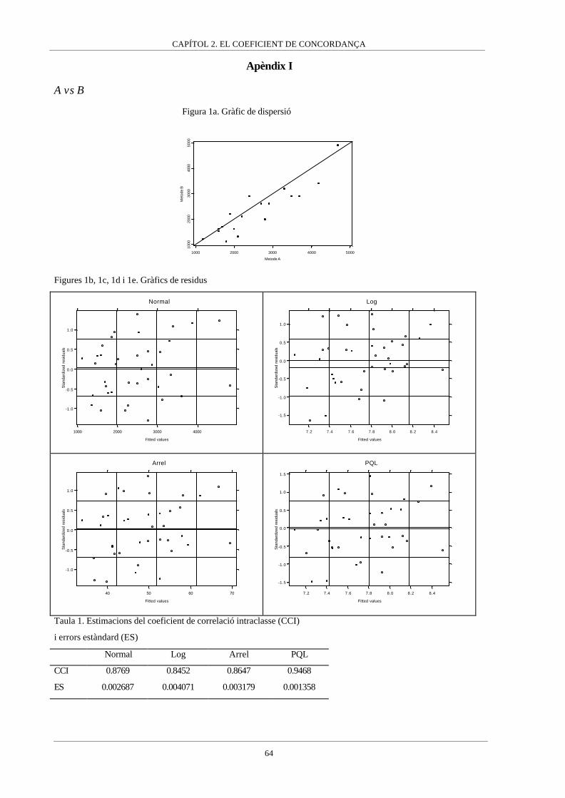
CAPÍTOL 2. EL COEFICIENT DE CONCORDANÇA
64
Apèndix I
A vs B
Figura 1a. Gràfic de dispersió
1000 2000 3000 4000 5000
Metode A
1000
2000
3000
4000
5000
Met
ode
B
Figures 1b, 1c, 1d i 1e. Gràfics de residus
-1.0
-0.5
0.0
0.5
1.0
1000 2000 3000 4000
Fitted values
Sta
ndar
dize
d re
sidu
als
Normal
-1.5
-1.0
-0.5
0.0
0.5
1.0
7.2 7.4 7.6 7.8 8.0 8.2 8.4
Fitted values
Sta
ndar
dize
d re
sidu
als
Log
-1.0
-0.5
0.0
0.5
1.0
40 50 60 70
Fitted values
Sta
ndar
dize
d re
sidu
als
Arrel
-1.5
-1.0
-0.5
0.0
0.5
1.0
1.5
7.2 7.4 7.6 7.8 8.0 8.2 8.4
Fitted values
Sta
ndar
dize
d re
sidu
als
PQL
Taula 1. Estimacions del coeficient de correlació intraclasse (CCI)
i errors estàndard (ES)
Normal Log Arrel PQL
CCI 0.8769 0.8452 0.8647 0.9468
ES 0.002687 0.004071 0.003179 0.001358

CAPÍTOL 2. EL COEFICIENT DE CONCORDANÇA
65
A vs C
Figura 2a. Gràfic de dispersió
1000 2000 3000 4000 5000 6000
Metode A
1000
2000
3000
4000
5000
6000
Met
ode
C
Figures 2b, 2c, 2d i 2e. Gràfics de residus
-1.5
-1.0
-0.5
0.0
0.5
1.0
1.5
2000 3000 4000 5000 6000
Fitted values
Sta
ndar
dize
d re
sidu
als
Normal
-2
-1
0
1
7.4 7.6 7.8 8.0 8.2 8.4 8.6
Fitted values
Sta
ndar
dize
d re
sidu
als
Log
-1.5
-1.0
-0.5
0.0
0.5
1.0
1.5
40 50 60 70
Fitted values
Sta
ndar
dize
d re
sidu
als
Arrel
-1.5
-1.0
-0.5
0.0
0.5
1.0
7.4 7.6 7.8 8.0 8.2 8.4 8.6 8.8
Fitted values
Sta
ndar
dize
d re
sidu
als
PQL
Taula 2. Estimacions del coeficient de correlació intraclasse (CCI)
i errors estàndard (ES)
Normal Log Arrel PQL
CCI 0.5706 0.5672 0.5793 0.6326
ES 0.013335 0.013660 0.012815 0.011113

CAPÍTOL 2. EL COEFICIENT DE CONCORDANÇA
66
A vs D
Figura 3a. Gràfic de dispersió
2000 3000 4000 5000
Metode A
2000
3000
4000
5000
Met
ode
D
Figures 3b, 3c, 3d i 3e. Gràfics de residus
-2
-1
0
1
2
2000 3000 4000 5000
Fitted values
Sta
ndar
dize
d re
sidu
als
Normal
-2
-1
0
1
7.4 7.6 7.8 8.0 8.2 8.4
Fitted values
Sta
ndar
dize
d re
sidu
als
Log
-1
0
1
2
40 45 50 55 60 65 70
Fitted values
Sta
ndar
dize
d re
sidu
als
Arrel
-1
0
1
2
7.4 7.6 7.8 8.0 8.2 8.4
Fitted values
Sta
ndar
dize
d re
sidu
als
PQL
Taula 3. Estimacions del coeficient de correlació intraclasse (CCI)
i errors estàndard (ES)
Normal Logaritme Arrel PQL
CCI 0.7601 0.7331 0.7539 0.8844
ES 0.008381 0.010184 0.008791 0.005032
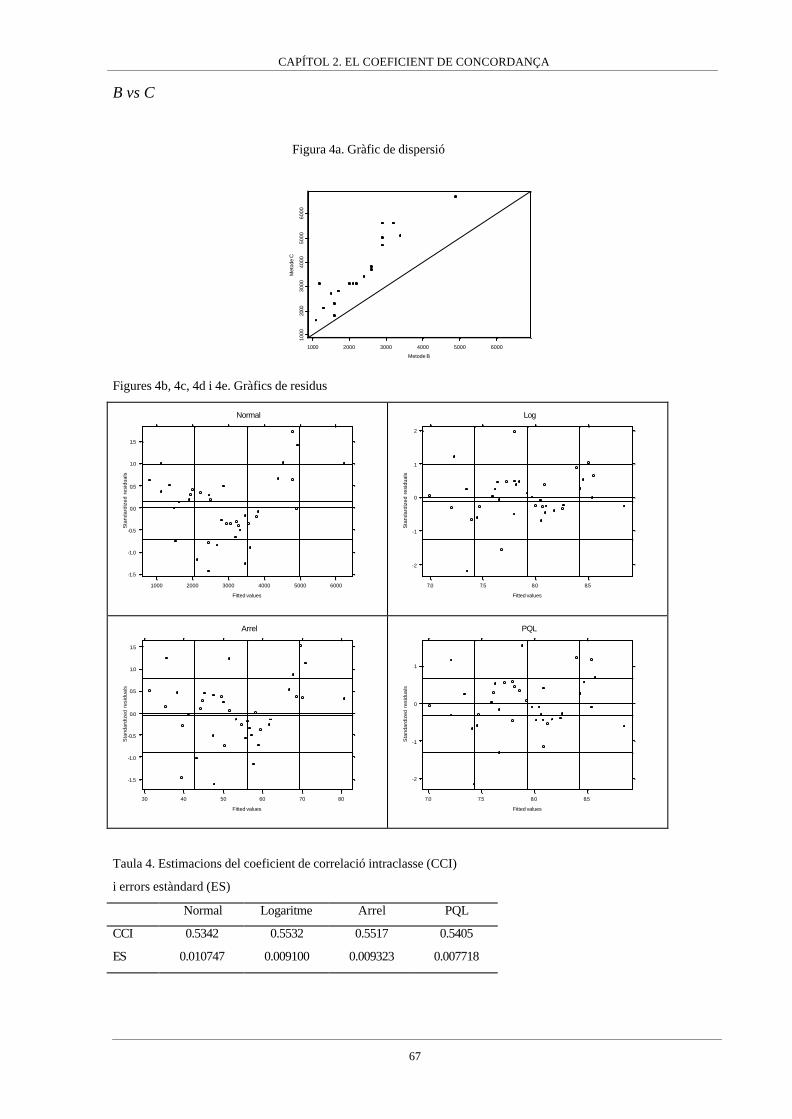
CAPÍTOL 2. EL COEFICIENT DE CONCORDANÇA
67
B vs C
Figura 4a. Gràfic de dispersió
1000 2000 3000 4000 5000 6000
Metode B
1000
2000
3000
4000
5000
6000
Met
ode
C
Figures 4b, 4c, 4d i 4e. Gràfics de residus
-1.5
-1.0
-0.5
0.0
0.5
1.0
1.5
1000 2000 3000 4000 5000 6000
Fitted values
Sta
ndar
dize
d re
sidu
als
Normal
-2
-1
0
1
2
7.0 7.5 8.0 8.5
Fitted values
Sta
ndar
dize
d re
sidu
als
Log
-1.5
-1.0
-0.5
0.0
0.5
1.0
1.5
30 40 50 60 70 80
Fitted values
Sta
ndar
dize
d re
sidu
als
Arrel
-2
-1
0
1
7.0 7.5 8.0 8.5
Fitted values
Sta
ndar
dize
d re
sidu
als
PQL
Taula 4. Estimacions del coeficient de correlació intraclasse (CCI)
i errors estàndard (ES)
Normal Logaritme Arrel PQL
CCI 0.5342 0.5532 0.5517 0.5405
ES 0.010747 0.009100 0.009323 0.007718
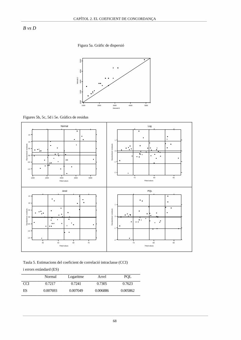
CAPÍTOL 2. EL COEFICIENT DE CONCORDANÇA
68
B vs D
Figura 5a. Gràfic de dispersió
1000 2000 3000 4000 5000
Metode B
1000
2000
3000
4000
5000
Met
ode
D
Figures 5b, 5c, 5d i 5e. Gràfics de residus
-1.0
-0.5
0.0
0.5
1.0
1.5
1000 2000 3000 4000 5000
Fitted values
Sta
ndar
dize
d re
sidu
als
Normal
-2
-1
0
1
7.5 8.0 8.5
Fitted values
Sta
ndar
dize
d re
sidu
als
Log
-1.5
-1.0
-0.5
0.0
0.5
1.0
1.5
40 50 60 70
Fitted values
Sta
ndar
dize
d re
sidu
als
Arrel
-2
-1
0
1
7.5 8.0 8.5
Fitted values
Sta
ndar
dize
d re
sidu
als
PQL
Taula 5. Estimacions del coeficient de correlació intraclasse (CCI)
i errors estàndard (ES)
Normal Logaritme Arrel PQL
CCI 0.7217 0.7241 0.7305 0.7623
ES 0.007693 0.007049 0.006886 0.005862

CAPÍTOL 2. EL COEFICIENT DE CONCORDANÇA
69
C vs D
Figura 6a. Gràfic de dispersió
2000 3000 4000 5000 6000
Metode C
2000
3000
4000
5000
6000
Met
ode
D
Figures 6b, 6c, 6d i 6e. Gràfics de residus
-1
0
1
2
2000 3000 4000 5000 6000
Fitted values
Sta
ndar
dize
d re
sidu
als
Normal
-1.5
-1.0
-0.5
0.0
0.5
1.0
1.5
7.4 7.6 7.8 8.0 8.2 8.4 8.6
Fitted values
Sta
ndar
dize
d re
sidu
als
Log
-1
0
1
2
40 50 60 70
Fitted values
Sta
ndar
dize
d re
sidu
als
Arrel
-1
0
1
7.4 7.6 7.8 8.0 8.2 8.4 8.6 8.8
Fitted values
Sta
ndar
dize
d re
sidu
als
PQL
Taula 6. Estimacions del coeficient de correlació intraclasse (CCI)
i errors estàndard (ES)
Normal Logaritme Arrel PQL
CCI 0.8006 0.8298 0.8205 0.8738
ES 0.005470 0.004052 0.004454 0.002951

CAPÍTOL 2. EL COEFICIENT DE CONCORDANÇA
70

CAPÍTOL 2. EL COEFICIENT DE CONCORDANÇA
71
Apèndix II
Quantiles of Standard Normal
Sta
ndar
ized
IC
C
-4 -2 0 2 4
-4-2
02
4Combination 1 n=30
Quantiles of Standard Normal
Sta
ndar
ized
IC
C
-4 -2 0 2 4
-4-2
02
4
Combination 1 n=100
Quantiles of Standard Normal
Sta
ndar
ized
IC
C
-4 -2 0 2 4
-4-2
02
4
Combination 2 n=30
Quantiles of Standard Normal
Sta
ndar
ized
IC
C
-4 -2 0 2 4
-4-2
02
4
Combination 2 n=100
Quantiles of Standard Normal
Sta
ndar
ized
IC
C
-4 -2 0 2 4
-4-2
02
4
Combination 3 n=30
Quantiles of Standard Normal
Sta
ndar
ized
IC
C
-4 -2 0 2 4
-4-2
02
4
Combination 3 n=100
Quantiles of Standard Normal
Sta
ndar
ized
IC
C
-4 -2 0 2 4
-4-2
02
4
Combination 4 n=30
Quantiles of Standard Normal
Sta
ndar
ized
IC
C
-4 -2 0 2 4
-4-2
02
4
Combination 4 n=100
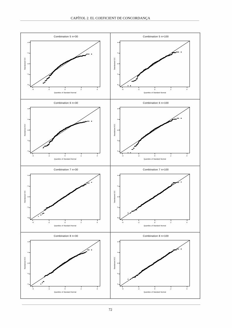
CAPÍTOL 2. EL COEFICIENT DE CONCORDANÇA
72
Quantiles of Standard Normal
Sta
ndar
ized
IC
C
-4 -2 0 2 4
-4-2
02
4
Combination 5 n=30
Quantiles of Standard Normal
Sta
ndar
ized
IC
C
-4 -2 0 2 4
-4-2
02
4
Combination 5 n=100
Quantiles of Standard Normal
Sta
ndar
ized
IC
C
-4 -2 0 2 4
-4-2
02
4
Combination 6 n=30
Quantiles of Standard Normal
Sta
ndar
ized
IC
C
-4 -2 0 2 4
-4-2
02
4
Combination 6 n=100
Quantiles of Standard Normal
Sta
ndar
ized
IC
C
-4 -2 0 2 4
-4-2
02
4
Combination 7 n=30
Quantiles of Standard Normal
Sta
ndar
ized
IC
C
-4 -2 0 2 4
-4-2
02
4
Combination 7 n=100
Quantiles of Standard Normal
Sta
ndar
ized
IC
C
-4 -2 0 2 4
-4-2
02
4
Combination 8 n=30
Quantiles of Standard Normal
Sta
ndar
ized
IC
C
-4 -2 0 2 4
-4-2
02
4
Combination 8 n=100

CAPÍTOL 2. EL COEFICIENT DE CONCORDANÇA
73
Quantiles of Standard Normal
Sta
ndar
ized
IC
C
-4 -2 0 2 4
-4-2
02
4Combination 9 n=30
Quantiles of Standard Normal
Sta
ndar
ized
IC
C
-4 -2 0 2 4
-4-2
02
4
Combination 9 n=100
Quantiles of Standard Normal
Sta
ndar
ized
IC
C
-4 -2 0 2 4
-4-2
02
4
Combination 10 n=30
Quantiles of Standard Normal
Sta
ndar
ized
IC
C
-4 -2 0 2 4
-4-2
02
4
Combination 10 n=100
Quantiles of Standard Normal
Sta
ndar
ized
IC
C
-4 -2 0 2 4
-4-2
02
4
Combination 11 n=30
Quantiles of Standard Normal
Sta
ndar
ized
IC
C
-4 -2 0 2 4
-4-2
02
4
Combination 11 n=100
Quantiles of Standard Normal
Sta
ndar
ized
IC
C
-4 -2 0 2 4
-4-2
02
4
Combination 12 n=30
Quantiles of Standard Normal
Sta
ndar
ized
IC
C
-4 -2 0 2 4
-4-2
02
4
Combination 12 n=100

CAPÍTOL 2. EL COEFICIENT DE CONCORDANÇA
74
Quantiles of Standard Normal
Sta
ndar
ized
Z
-4 -2 0 2 4
-4-2
02
4
Combination 1 n=30
Quantiles of Standard Normal
Sta
ndar
ized
Z
-4 -2 0 2 4
-4-2
02
4
Combination 1 n=100
Quantiles of Standard Normal
Sta
ndar
ized
Z
-4 -2 0 2 4
-4-2
02
4
Combination 2 n=30
Quantiles of Standard Normal
Sta
ndar
ized
Z
-4 -2 0 2 4
-4-2
02
4
Combination 2 n=100
Quantiles of Standard Normal
Sta
ndar
ized
Z
-4 -2 0 2 4
-4-2
02
4
Combination 3 n=30
Quantiles of Standard Normal
Sta
ndar
ized
Z
-4 -2 0 2 4
-4-2
02
4
Combination 3 n=100
Quantiles of Standard Normal
Sta
ndar
ized
Z
-4 -2 0 2 4
-4-2
02
4
Combination 4 n=30
Quantiles of Standard Normal
Sta
ndar
ized
Z
-4 -2 0 2 4
-4-2
02
4
Combination 4 n=100

CAPÍTOL 2. EL COEFICIENT DE CONCORDANÇA
75
-4 -2 0 2 4
Quantiles of Standard Normal
-4-2
02
4
Sta
ndar
ized
ZCombination 5 n=30
-4 -2 0 2 4
Quantiles of Standard Normal
-4-2
02
4
Sta
ndar
ized
Z
Combination 5 n=100
Quantiles of Standard Normal
Sta
ndar
ized
Z
-4 -2 0 2 4
-4-2
02
4
Combination 6 n=30
Quantiles of Standard Normal
Sta
ndar
ized
Z
-4 -2 0 2 4
-4-2
02
4
Combination 6 n=100
Quantiles of Standard Normal
Sta
ndar
ized
Z
-4 -2 0 2 4
-4-2
02
4
Combination 7 n=30
Quantiles of Standard Normal
Sta
ndar
ized
Z
-4 -2 0 2 4
-4-2
02
4
Combination 7 n=100
Quantiles of Standard Normal
Sta
ndar
ized
Z
-4 -2 0 2 4
-4-2
02
4
Combination 8 n=30
Quantiles of Standard Normal
Sta
ndar
ized
Z
-4 -2 0 2 4
-4-2
02
4
Combination 8 n=100

CAPÍTOL 2. EL COEFICIENT DE CONCORDANÇA
76
Quantiles of Standard Normal
Sta
ndar
ized
Z
-4 -2 0 2 4
-4-2
02
4
Combination 9 n=30
Quantiles of Standard Normal
Sta
ndar
ized
Z
-4 -2 0 2 4
-4-2
02
4
Combination 9 n=100
Quantiles of Standard Normal
Sta
ndar
ized
Z
-4 -2 0 2 4
-4-2
02
4
Combination 10 n=30
Quantiles of Standard Normal
Sta
ndar
ized
Z
-4 -2 0 2 4
-4-2
02
4
Combination 10 n=100
Quantiles of Standard Normal
Sta
ndar
ized
Z
-4 -2 0 2 4
-4-2
02
4
Combination 11 n=30
Quantiles of Standard Normal
Sta
ndar
ized
Z
-4 -2 0 2 4
-4-2
02
4
Combination 11 n=100
Quantiles of Standard Normal
Sta
ndar
ized
Z
-4 -2 0 2 4
-4-2
02
4
Combination 12 n=30
Quantiles of Standard Normal
Sta
ndar
ized
Z
-4 -2 0 2 4
-4-2
02
4
Combination 12 n=100

CAPÍTOL 2. EL COEFICIENT DE CONCORDANÇA
77

CAPÍTOL 3. EL MODEL D’EQUACIÓ ESTRUCTURAL APLICAT A BIOEQUIVALÈNCIA
78
CAPÍTOL 3
CAPÍTOL 3. EL MODEL D’EQUACIÓ ESTRUCTURAL APLICAT A BIOEQUIVALÈNCIA
79
EL MODEL D’EQUACIÓ ESTRUCTURAL APLICAT A BIOEQUIVALÈNCIA
Introducció
En l’àmbit de la indústria farmacèutica, quan hom desitja introduir un nou producte terapèutic en
el mercat s’ha de demostrar que té l’efectivitat desitjada i els nivells de tolerància indicats per les
autoritats competents. Això implica la realització d’un assaig clínic que pot ser molt costós tant
en termes econòmics com en temps de realització.
Es podria donar el cas de que el nou producte sigui una nova formulació d’un producte (principi
actiu) ja existent en el mercat. Aquest fet es pot presentar en dues formes: com a equivalència
farmacèutica o com a alternativa farmacèutica (EMEA, 2000). El nou producte és
farmacèuticament equivalent si conté la mateixa quantitat de la mateixa substància activa en la
mateixa forma de dosificació que es troba en el producte de referència, per exemple dos
productes de paracetamol presentats en càpsules de 500 mg. En canvi, el producte serà una
alternativa farmacèutica si estant composat pel mateix principi actiu difereix en la forma química
o en la forma de dosificació. Continuant amb l’exemple del paracetamol, una alternativa
farmacèutica a la càpsula de 500 mg seria una presentació efervescent del paracetamol en una
quantitat de 500 mg.
El fet de que existeixi un producte de referència pel qual l’eficàcia i seguretat ja han estat
demostrades pot facilitar la introducció del nou producte, ja sigui equivalència o alternativa
farmacèutica. Això es deu a que hom considera que el nou producte és equivalent en seguretat i
eficàcia al producte de referència si la seva biodisponibilitat és la mateixa, essent la
biodisponibilitat la velocitat i extensió amb la que la substància o principi actiu és absorbit i
resulta disponible en el lloc d’acció. El procediment per a demostrar la igualtat de
biodisponibilitats entre els dos productes és conegut com a assaig de bioequivalència, en el que la
biodisponibilitat dels dos productes es mesurada a una sèrie de voluntaris “sans”, habitualment
sota un disseny creuat. Per tant l’objectiu de l’assaig de bioequivalència és demostrar igualtat de
biodisponibilitat per poder demostrar d’una forma relativament ràpida que el nou producte és
efectiu i segur, o almenys tant efectiu i segur com el producte de referència.
La biodisponibilitat es mesura utilitzant una corba farmacocinètica (Figura 1), en la qual es
representa en el eix d’abscisses el temps transcorregut i en l’eix d’ordenades la concentració en

CAPÍTOL 3. EL MODEL D’EQUACIÓ ESTRUCTURAL APLICAT A BIOEQUIVALÈNCIA
80
sang del fàrmac. La biodisponibilitat s’expressa com una mesura resum d’aquesta corba, essent
les mesures més utilitzades l’àrea sota la corba (AUC), la concentració màxima (Cmax) i el
moment en que s’arriba a la concentració màxima (Tmax).
Figura 1. Corba farmacocinètica.
0 5 10 15 20Temps
0.00
0.02
0.04
0.06
0.08
0.10
0.12
0.14
Con
cent
raci
ó
AUC
TmaxTmax
Cmax
Suposem que a una mostra de n individus se’ls ha mesurat la biodisponibilitat de cada producte k
vegades. El model de mesura que s’assumeix pel logaritme de les biodisponibilitats és el següent
(Schall and Luus, 1993)
RijRiRij
TijTiTij
euR
euT
++µ=
++µ=, i=1,...,n, j=1,...,k
on R i T representen els productes de referència i a testar respectivament, µT i µR són les mitjanes
globals de log-biodisponibilitats de cada producte, uTi i uRi són les desviacions en mitjana respecte
les mitjanes globals corresponents a l’individu i-èssim, és a dir, l’efecte individu. Finalment eTij,
eRij són les desviacions de la mesura j-èssima respecte les mitjanes de l’individu i-èssim, això és,
les variacions intra-individu.
S’assumeix que tant els efectes individu com les desviacions intra-individu és distribueixen sota
distribucions normals. Així, ( )BTiT ,0N~u σ , ( )BRRi ,0N~u σ , ( )WTTij ,0N~e σ , ( )WRRij ,0N~e σ .
També s’assumeix que les úniques components del model que covarien són els efectes individu,
( ) RTTiRi u,ucov σ= .
CAPÍTOL 3. EL MODEL D’EQUACIÓ ESTRUCTURAL APLICAT A BIOEQUIVALÈNCIA
81
S’han definit tres tipus de bioequivalència (Anderson and Hauck, 1990): bioequivalència en
mitjana, bioequivalència poblacional i bioequivalència individual. La bioequivalència en mitjana
és el tipus més utilitzat i que actualment és exigit en la majoria d’agències farmacèutiques.
Aquesta es dona quan existeix igualtat de mitjanes globals, RT µ=µ . Per tant, si existeix
bioequivalència en mitjana, els dos productes tindran en mitjana la mateixa biodisponibilitat a la
població d’estudi.
La bioequivalència poblacional requereix igualtat de mitjanes globals i igualtat de les variàncies
totals de cada mètode, 2T
2R σ=σ , on 2
WR2BR
2R σ+σ=σ i 2
TR2BT
2T σ+σ=σ . La igualtat de mitjanes i
variàncies junt amb l’assumpció de normalitat implica que les distribucions de densitat de
probabilitat marginals de les log-biodisponibilitats seran iguals. Per tant, la bioequivalència
poblacional garanteix que les biodisponibilitats dels dos productes es distribueixen igual en la
població d’estudi. Aquest tipus de bioequivalència es troba relacionat amb el concepte de
"prescribilitat” (prescribability), és a dir, quan el clínic ha decidir entre els dos productes per
iniciar un tractament. En el cas de que siguin poblacionalment bioequivalents al metge li serà
indiferent prescriure un o altre, perquè a priori els dos productes tenen la mateixa distribució de
probabilitat sobre la quantitat de biodisponibilitat que serà aconseguida en els individus de la
població de pacients.
Finalment, la bioequivalència individual requereix igualtat de log-biodisponibilitats per a
qualsevol individu. Això implica igualtat de mitjanes globals, igualtat de mitjanes individuals,
TiRi uu = , i que la variabilitat de les desviacions intra-individu siguin iguals, 2WT
2WR σ=σ . Sota
l’assumpció de normalitat dels efectes, la bioequivalència individual implica igualtat de les
distribucions de densitat de probabilitat condicionades als individus de les log-biodisponibilitats.
Suposem que un individu concret ha iniciat un tractament amb el producte de referència i en un
moment donat el clínic vol canviar el tractament pel producte a testar. Si els dos productes són
individualment bioequivalents es pot assumir que la quantitat de principi actiu que serà
biodisponible per aquell individu en concret serà la mateixa independentment del producte que
s’utilitzi. Per aquesta raó la bioequivalència individual es relaciona amb el concepte de
intercanviabilitat (switchability) entre els dos tractaments, es a dir, en qualsevol moment del
tractament es pot utilitzar un o altre producte indistintament perquè a priori els dos productes
tenen la mateixa distribució de probabilitat, condicionada a l’individu, sobre la quantitat de
biodisponibilitat que serà aconseguida.
CAPÍTOL 3. EL MODEL D’EQUACIÓ ESTRUCTURAL APLICAT A BIOEQUIVALÈNCIA
82
Els tres tipus de bioequivalència tenen una característica comú: és necessari demostrar la igualtat
entre productes. En realitat demostrar igualtat és una prova determinista: només cal esperar fins
trobar una diferència i la igualtat serà rebutjada. Per això és més interessant i útil parlar
d’equivalència, són els paràmetres prou semblants o les seves distribucions de probabilitats prou
similars per considerar-los equivalents? La resposta a aquesta pregunta passa per definir uns
límits a partir dels quals es considerarà que la diferència és massa gran com per assumir
equivalència.
A més a més, el contrast d’hipòtesi clàssic resulta inadequat per demostrar equivalència
(Westlake, 1972). Això es degut a que si s’utilitza la hipòtesi nul·la d’igualtat estricta, H0: µR=µT ,
i es controla l’error de tipus I associat, el que en realitat s’estarà controlant és la probabilitat de
declarar erròniament inequivalència, quan el més apropiat és controlar l’error al declarar
equivalència. Seria possible realitzar-ho controlant l’error de tipus II, però en lloc d’equivalència
s’estaria intentant demostrar igualtat. Per tant, és necessari buscar una metodologia diferent que
permeti avaluar l’equivalència.
El procediment més acceptat per testar hipòtesis genèriques d’equivalència és el two-one sided
test approach (Schuirmann, 1987) en el que el problema és formulat mitjançant dues hipòtesis.
Suposem que es declararà que les mitjanes són equivalents si la diferència en valor absolut entre
elles és menor que un cert valor δ . La primera hipòtesi alternativa a testar és que la diferència
entre les mitjanes sigui menor que δ , mentre que a la segona hipòtesi alternativa és que la
diferència sigui superior a -δ. Si ambdues hipòtesis nul·les són rebutjades amb una probabilitat
d’error de tipus I fixada a α, es declararà equivalència amb una probabilitat d’error igual a α .
Aquest procediment és idèntic a construir un interval de confiança amb una confiança del
( α− 21 )% i comprovar si l’interval cau completament dintre de l’interval d’equivalència ( )δδ− , .
El procediment two one-sided test s’ha aplicat principalment en l’assaig de bioequivalència en
mitjana degut a que es tracta del procediment recomanat per les agències europees i americanes.
No obstant s’han proposat altres mètodes per avaluar la bioequivalència en mitjana, alguns basats
també en la construcció d’intervals de confiança de la diferència de mitjanes (Westlake, 1976;
Kirkwood, 1981) i d’altres en procediments més sofisticats com el proposat per Lindley (1998)
que utilitza una funció de pèrdua. Cal destacar el mètode anomenat regla del 75/75, on s’exigeix
que el quocient entre les mesures de biodisponibilitats dels productes de referència i a testar ha
d’estar entre 0.75 i 1.25, i que això s’ha de complir en almenys el 75% dels individus. Aquesta

CAPÍTOL 3. EL MODEL D’EQUACIÓ ESTRUCTURAL APLICAT A BIOEQUIVALÈNCIA
83
regla no s’ha utilitzat gaire perquè va ser criticada pel pobre comportament estadístic que donava,
tot i que per una banda el criteri del quocient es va mantenir com a límits de bioequivalència per
la bioequivalència en mitjana, i per altre el criteri de que la regla es compleixi en un cert
percentatge de la població ha tornat a ser considerat pel cas de la bioequivalència individual.
Els altres dos tipus de bioequivalència, poblacional i individual, s’han qualificat con més
restrictives que la bioequivalència en mitjana perquè es veuen més paràmetres implicats en la
demostració d’equivalència. Per tant, sota aquesta perspectiva el tipus de bioequivalència més
restrictiu és la individual. El fet de què s’hagin d’avaluar diferents paràmetres a banda de les
mitjanes globals ha fet que els procediments proposats s’hagin classificat en agregats i
desagregats (Chen, 1997), on un procediment agregat avalua la bioequivalència combinant tots
els paràmetres implicats en un únic índex. Pel contrari, un mètode desagregat avalua per separat
cadascun dels paràmetres involucrats en la bioequivalència. Actualment el procediment proposat
per la Food and Drug Administration tan per bioequivalència poblacional com individual és
agregat (FDA, 2001), donat que combina les mitjanes i les variàncies totals per la bioequivalència
poblacional, i per la bioequivalència individual utilitza alhora les mitjanes globals, les variàncies
intra-individu i la variància de la diferència entre les mitjanes individuals anomenada variància de
la interacció individu-formulació. No obstant, en els darrers anys diversos mètodes de diferent
naturalesa han estat proposats (Holder and Hsuan, 1993; Esinhart and Chinchilli, 1994; Vuorinen
and Turunen, 1996; Gould, 2000; Lin, 2000) posant de manifest que la bioequivalència encara és
un tema candent origen de força discussió.
En aquest capítol de la memòria ens centrarem en la demostració de bioequivalència individual.
Així el primer article mostra el procediment actualment proposat per la FDA (2001) i es presenta
el model d’equació estructural com una alternativa vàlida per a la avaluació de bioequivalencia
individual. El model d’equació estructural assumeix que la relació entre les mitjanes individuals
de cada producte és la mateixa per a tots els individus, per relaxar aquesta assumpció una
extensió d’aquest model, el model d’equació estructural error-in-equation, es presentat en el
segon article.

CAPÍTOL 3. EL MODEL D’EQUACIÓ ESTRUCTURAL APLICAT A BIOEQUIVALÈNCIA
84
CAPÍTOL 3. EL MODEL D’EQUACIÓ ESTRUCTURAL APLICAT A BIOEQUIVALÈNCIA
85
Assessing individual bioequivalence using the structural
equation model
Josep-Lluís Carrasco and Lluís Jover
Bioestadística, Departament de Salut Pública, Universitat de Barcelona, Barcelona, Spain
SUMMARY
The structural equation model (SEM) is introduced as a useful approach for assessing individual bioequivalence.
SEM parameters are estimated using a partial likelihood analysis and the hypothesis of individual bioequivalence is
evaluated in a disaggregate way, testing separately the hypothesis concerning SEM parameters, and assessing the
overall hypothesis of individual bioequivalence using the intersection-union principle. Limits of bioequivalence for
SEM parameters are proposed and a power analysis is carried out.
KEYWORDS: Individual bioequivalence, structural equation model, intersection-union principle, partial
likelihood analysis, limits of bioequivalence
1. INTRODUCTION
The aim of bioequivalence trials is to show that two formulations have similar bioavailabilities.
Originally, bioequivalence assays implied equality of average bioavailabilit ies, but Anderson and
Hauck [1] demonstrated that this equality was insufficient to guarantee switchability between
formulations, and so they defined the concept of individual bioequivalence. The FDA has now
incorporated an aggregate index in its guidelines [2], based on the procedures of Schall and Luus
[3] and Hyslop et al. [4]. This index simultaneously measures departures from three issues:
equality of means, equality of within-subject variances and absence of subject-by-formulation
interaction variance. Since the concept of “similar bioavailabilities” actually means agreement
between the bioavailabilities of two formulations, the procedures used in agreement problems
seem adequate in individual bioequivalence assays. We will introduce the structural equation
model (SEM) as an approach used in reliability and method comparison assays [5], and as a
useful disaggregate approach for testing individual bioequivalence [6, 7]. Section 2 contains the
measurement model for bioavailabilities and a brief description of the current FDA criterion for
assessing individual bioequivalence. Section 3 illustrates the SEM approach, including parameter
estimation, hypotheses concerning individual bioequivalence and the bioequivalent limits used to
test these hypotheses. A case-example is given in section 4 comparing the SEM approach with
CAPÍTOL 3. EL MODEL D’EQUACIÓ ESTRUCTURAL APLICAT A BIOEQUIVALÈNCIA
86
the method currently recommended by the FDA. Finally, section 5 contains the discussion and
main conclusions about the characteristics of SEM as a tool for assessing individual
bioequivalence
2. THE FDA’S APPROACH
2.1 Measurement model
Analyses of individual bioequivalence are typically based on models of the logarithm of
bioavailability measurements. The most common measures of bioavailabilities are derived from a
pharmacokinetic curve: the area under the concentration curve (AUC) or the maximum
concentration (Cmax). The measurement model proposed for bioavailabilities (or its log-
transformed values) by Schall and Luus [3] is
RijRiRijTijTiTij euReuT ++µ=++µ=
where Tij and Rij are the bioavailabilities of tested (T) and reference (R) formulations, µT and µR
are the overall averages of T and R, uTi and uRi are the mean deviations of individual i and eTij and
eRij are the deviations of individual i on j determination, with i=1,..,n and j=1,...,k. It is assumed
that ( )BTiT ,0N~u σ , ( )BRRi ,0N~u σ , ( )WTTij ,0N~e σ , ( )WRRij ,0N~e σ
The individual bioequivalence is completely achieved (T and R are bio-identical) when TR µ=µ ,
2WT
2WR σ=σ and 02
D =σ , where 2Dσ is the variance of the subject-by-formulation interaction and
can be expressed as ( ) RT2BR
2BTRiTi
2D 2uuVar σ−σ+σ=−=σ .
2.2 Criterion and bioequivalent limits
The FDA’s criterion is based on the following index ( ) ( )( ) I2
0W2WR
2WR
2WT
2D
2
RT
,maxθ≤
σσσ−σ+σ+µ−µ
=θ [2],
where 20Wσ is a constant with a suggested value of 0.04, and
Iθ is the bioequivalent limit with a
recommended value of ( )5.24948.2
04.005.025.1ln 2
I ≈=+=θ , being ( )225.1ln the limit for the
difference of average, 0.05 is the limit obtained from the addition of within-subject variances
difference (0.02) and the subject-by-formulation interaction variance (0.03) limits, and 0.04
comes from 20Wσ . According to the value used in the denominator, 2
WRσ or 2WOσ , the index θ is
called either “reference scaled” or “constant scaled”, respectively.
CAPÍTOL 3. EL MODEL D’EQUACIÓ ESTRUCTURAL APLICAT A BIOEQUIVALÈNCIA
87
This index is considered to be an aggregate measure because it evaluates averages difference,
within-subject variances difference and the subject-by-formulation interaction variance at the
same time. The bioequivalence is accepted at significance level α if the ( )%1 α− upper
confidence limit of θ is lower than Iθ . Hyslop et al. [4] have recently proposed a linearized
version of the criterion, where the index becomes
( ) ( ) ( )20W
2WRI
2WR
2WT
2D
2
RT ,max σσ⋅θ−σ−σ+σ+µ−µ=η , concluding bioequivalence if the
( )%1 α− upper confidence limit of η is lower than 0.
3. STRUCTURAL EQUATION MODEL
3.1 The model
The structural equation model (SEM) uses the same measurement model proposed above, but for
the sake of simplicity we are expressing it as RijRiijTijTiij euReuT +=+= where it is assumed
that ( )BTTiT ,N~u σµ , ( )BRRRi ,N~u σµ , ( )WTTij ,0N~e σ , ( )WRRij ,0N~e σ and the only
covariance among components of the model that is not equal to zero is ( ) RTTiRi u,ucov σ= .
The SEM incorporates a new component in the model, the structural relationship between uTi and
uRi, defined as RiTi uu ⋅β+α= [8], therefore we are adding the assumption that the individual
averages have a linear relationship. Assuming this model, we are modelling the relationship
between means of both formulations and the covariance structure of individual effects, and hence
we have 2BRRT
2BR
22BTRT ;; σ⋅β=σσβ=σµ⋅β+α=µ and ( ) RRT 1 µ⋅−β+α=µ−µ=ϕ
and therefore, if α, β , 2WT
2WR , σσ , 2
BRσ and Rµ are known the model is completely specified. We
can also rewrite 2Dσ and express it as
( ) ( ) 2BR
22BR
2BR
2BR
2RT
2BR
2BTRT
2D 122uuVar σ⋅−β=σ⋅β⋅−σ+σ⋅β=σ⋅−σ+σ=−=σ
so now the individual bioequivalence is completely achieved when β = 1, α = 0 and
12WT
2WR =σσ=λ . These criteria can be relaxed in the same way as the FDA criterion and then
individual bioequivalence is accepted when [ ]21 ;θθ∈β , [ ]43 ;θθ∈ϕ and 5θ<λ , being
4321 ,,, θθθθ and 5θ the bioequivalent limits.
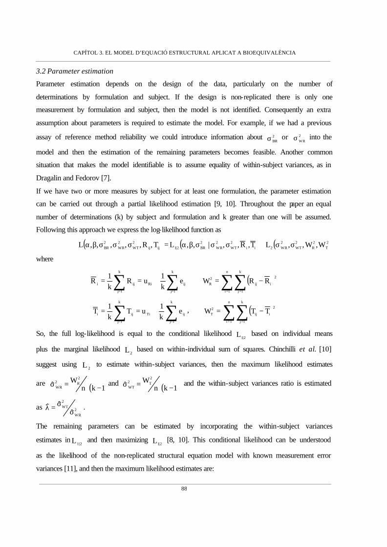
CAPÍTOL 3. EL MODEL D’EQUACIÓ ESTRUCTURAL APLICAT A BIOEQUIVALÈNCIA
88
3.2 Parameter estimation
Parameter estimation depends on the design of the data, particularly on the number of
determinations by formulation and subject. If the design is non-replicated there is only one
measurement by formulation and subject, then the model is not identified. Consequently an extra
assumption about parameters is required to estimate the model. For example, if we had a previous
assay of reference method reliability we could introduce information about 2BRσ or 2
WRσ into the
model and then the estimation of the remaining parameters becomes feasible. Another common
situation that makes the model identifiable is to assume equality of within-subject variances, as in
Dragalin and Fedorov [7].
If we have two or more measures by subject for at least one formulation, the parameter estimation
can be carried out through a partial likelihood estimation [9, 10]. Throughout the paper an equal
number of determinations (k) by subject and formulation and k greater than one will be assumed.
Following this approach we express the log-likelihood function as
( ) ( ) ( )2T
2R
2WT
2WR2ii
2WT
2WR
2BR2|1ijij
2WT
2WR
2BR W,W,,LT,R,,|,,LT,R,,,,,L σσ+σσσβα=σσσβα
where
∑∑==
+==k
1j
ijRi
k
1j
iji ek1
uRk1
R ( )∑∑= =
−=n
1i
k
1j
2
iij2
R RRW
∑∑==
+==k
1j
ijTi
k
1j
iji ek1
uTk1
T , ( )∑∑= =
−=n
1i
k
1j
2
iij2
T TTW
So, the full log-likelihood is equal to the conditional likelihood 2|1L based on individual means
plus the marginal likelihood 2L based on within-individual sum of squares. Chinchilli et al. [10]
suggest using 2L to estimate within-subject variances, then the maximum likelihood estimates
are ( )1knWˆ
2R2
WR −⋅=σ and ( )1knWˆ
2T2
WT −⋅=σ and the within-subject variances ratio is estimated
as 2WR
2WT
ˆˆˆ
σσ=λ .
The remaining parameters can be estimated by incorporating the within-subject variances
estimates in2|1L and then maximizing
2|1L [8, 10]. This conditional likelihood can be understood
as the likelihood of the non-replicated structural equation model with known measurement error
variances [11], and then the maximum likelihood estimates are:
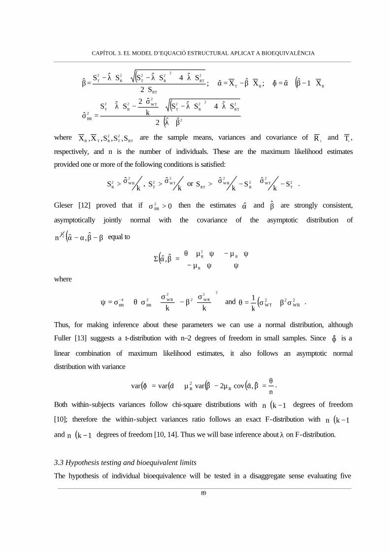
CAPÍTOL 3. EL MODEL D’EQUACIÓ ESTRUCTURAL APLICAT A BIOEQUIVALÈNCIA
89
( ) ( )
( )( )2
2RT
22R
2T
2WT2
R2T
2BR
RRT
RT
2RT
22R
2T
2R
2T
ˆˆ2
Sˆ4SˆSk
ˆ2SˆS
ˆ
X1ˆˆˆ;XˆXˆ;S2
Sˆ4SˆSSˆSˆ
β+λ⋅
⋅λ⋅+⋅λ−+σ⋅
−⋅λ+=σ
⋅−β+α=ϕ⋅β−=α⋅
⋅λ⋅+⋅λ−+⋅λ−=β
where RT
2T
2RTR S,S,S,X,X are the sample means, variances and covariance of
iR and iT ,
respectively, and n is the number of individuals. These are the maximum likelihood estimates
provided one or more of the following conditions is satisfied:
kˆS
2WR2
Rσ> , k
ˆS2WT2
Tσ> or
−σ
−σ> 2
T
2WT2
R
2WR
RT SkˆSk
ˆS .
Gleser [12] proved that if 02BR >σ then the estimates α and β are strongly consistent,
asymptotically jointly normal with the covariance of the asymptotic distribution of
( )β−βα−α ˆ,ˆn 21 equal to
( )
ψψ⋅µ−
ψ⋅µ−ψ⋅µ+θ=βαΣ
R
R2Rˆ,ˆ
where
σβ−
σ+σθ⋅σ=ψ −
22WR2
2WR2
BR4
BR kk and ( )2
WR22
WTk1
σβ+σ=θ .
Thus, for making inference about these parameters we can use a normal distribution, although
Fuller [13] suggests a t-distribution with n−2 degrees of freedom in small samples. Since ϕ is a
linear combination of maximum likelihood estimates, it also follows an asymptotic normal
distribution with variance
( ) ( ) ( ) ( )n
ˆ,ˆcov2ˆvarˆvarˆvar R2R
θ=βαµ−βµ+α=ϕ .
Both within-subjects variances follow chi-square distributions with ( )1kn −⋅ degrees of freedom
[10]; therefore the within-subject variances ratio follows an exact F-distribution with ( )1kn −⋅
and ( )1kn −⋅ degrees of freedom [10, 14]. Thus we will base inference about λ on F-distribution.
3.3 Hypothesis testing and bioequivalent limits
The hypothesis of individual bioequivalence will be tested in a disaggregate sense evaluating five
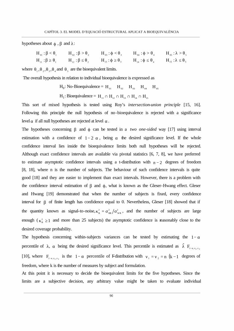
CAPÍTOL 3. EL MODEL D’EQUACIÓ ESTRUCTURAL APLICAT A BIOEQUIVALÈNCIA
90
hypotheses about ϕ , β and λ:
111
101
:H
:H
θ≥β
θ<β
212
202
:H
:H
θ≤β
θ>β
313
303
:H
:H
θ≥ϕ
θ<ϕ
414
404
:H
:H
θ≤ϕ
θ>ϕ
515
505
:H
:H
θ≤λ
θ>λ
where 4321 ,,, θθθθ and
5θ are the bioequivalent limits.
The overall hypothesis in relation to individual bioequivalence is expressed as
H0: No-Bioequivalence = 0504030201 HHHHH ∪∪∪∪
H1: Bioequivalence = 1514131211 HHHHH ∩∩∩∩
This sort of mixed hypothesis is tested using Roy’s intersection-union principle [15, 16].
Following this principle the null hypothesis of no-bioequivalence is rejected with a significance
level α if all null hypotheses are rejected at level α .
The hypotheses concerning β and ϕ can be tested in a two one-sided way [17] using interval
estimation with a confidence of α⋅− 21 , being α the desired significance level. If the whole
confidence interval lies inside the bioequivalence limits both null hypotheses will be rejected.
Although exact confidence intervals are available via pivotal statistics [6, 7, 8], we have preferred
to estimate asymptotic confidence intervals using a t-distribution with 2n − degrees of freedom
[8, 18], where n is the number of subjects. The behaviour of such confidence intervals is quite
good [18] and they are easier to implement than exact intervals. However, there is a problem with
the confidence interval estimation of β and ϕ, what is known as the Gleser-Hwang effect. Gleser
and Hwang [19] demonstrated that when the number of subjects is fixed, every confidence
interval for β of finite length has confidence equal to 0. Nevertheless, Gleser [18] showed that if
the quantity known as signal-to-noise, 2WR
2BR
2R σσ=κ , and the number of subjects are large
enough ( 12R ≥κ and more than 25 subjects) the asymptotic confidence is reasonably close to the
desired coverage probability.
The hypothesis concerning within-subjects variances can be tested by estimating the α−1
percentile of λ, α being the desired significance level. This percentile is estimated as 21 ,,1Fˆ
ννα−⋅λ
[10], where 21 ,,1F ννα− is the α−1 percentile of F-distribution with ( )1kn21 −⋅=ν=ν degrees of
freedom, where k is the number of measures by subject and formulation.
At this point it is necessary to decide the bioequivalent limits for the five hypotheses. Since the
limits are a subjective decision, any arbitrary value might be taken to evaluate individual

CAPÍTOL 3. EL MODEL D’EQUACIÓ ESTRUCTURAL APLICAT A BIOEQUIVALÈNCIA
91
bioequivalence, but we will try to adapt the FDA’s suggestions to SEM components. The limits
for averages difference are found from the well-known average bioequivalence inequality
( ) ( )22
RT 25.1ln≤µ−µ so the limits will be [ ]25.1ln,25.1ln ⋅−∈ϕ . The FDA considers a within-
subject standard deviation ratio to be large when it exceeds 1.5, so the limit for λ could be
25.25.1 2 = . For β we could use the fact that β links both between-subject variances, 2BR
2BT
22BR
22BT σσ=β→σβ=σ . Hence we could fix the limits in the within-subject variance way,
0 40 80 120
0.0
0.2
0.4
0.6
0.8
1.0
c1c2c3c4
a)
0 40 80 120
0.0
0.2
0.4
0.6
0.8
1.0
b)
c1c2c3c4
Figure 1. Power curves related to the null hypotheses of difference of means. a) 25.1log:H0 −<ϕ ; b) 25.1log:H0 >ϕ . Power corre sponds to Y-axis and X-axis represent the sample size. The parameters associated with each curve are shown in Table I.
so none of the between-subject standard deviations can exceed the other one by more than 50%
and this means the limits for β are [ ]5.1,32 .
These limits are an adaptation from FDA suggestions, but obviously it would be possible to find
other more or less restrictive limits, depending on the user’s requirements.
3.4 Power of the test
Berger and Hsu [20] pointed out that intersection-union test procedure can be quite conservative
with a type I error rate lower than would be desired. Initially, a low type I error rate is not an
undesirable property, but the difficulty in rejecting all H0 comes from the power of the test when
H0 is false. Since the power of the overall hypothesis of bioequivalence is the product of the
power of five hypotheses, it is worth studying the power of these hypotheses separately. For
example, if an overall power of 80% is desired it is necessary for each hypothesis to have a power
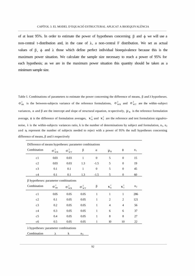
CAPÍTOL 3. EL MODEL D’EQUACIÓ ESTRUCTURAL APLICAT A BIOEQUIVALÈNCIA
92
of at least 95%. In order to estimate the power of hypotheses concerning β and ϕ we will use a
non-central t-distribution and, in the case of λ, a non-central F distribution. We set as actual
values of β, ϕ and λ those which define perfect individual bioequivalence because this is the
maximum power situation. We calculate the sample size necessary to reach a power of 95% for
each hypothesis; as we are in the maximum power situation this quantity should be taken as a
minimum sample size.
Table I. Combinations of parameters to estimate the power concerning the difference of means, β and λ hypotheses.
2BRσ is the between-subjects variance of the reference formulations, 2
WRσ and 2WTσ are the within -subject
variances, α and β are the intercept and slope of structural equation, re spectively, Rµ is the reference formulation
average, ϕ is the difference of formulation averages, 2Rκ and 2
Tκ are the reference and test formulation signal-to-
noise, λ is the within-subjects variances ratio, k is the number of determinations by subject and formulation, n1, n2
and n3 represent the number of subjects needed to reject with a power of 95% the null hypotheses concerning
difference of means, β and λ respectively
Difference of means hypotheses: parameter combinations
Combination 2WRσ 2
WTσ β α Rµ ϕ n1
c1 0.03 0.03 1 0 5 0 15
c2 0.03 0.03 1.3 -1.5 5 0 19
c3 0.1 0.1 1 0 5 0 45
c4 0.1 0.1 1.3 -1.5 5 0 60
β hypotheses: parameter combinations
Combination 2BRσ 2
WRσ 2WTσ β 2
Rκ 2Tκ n2
c1 0.05 0.05 0.05 1 1 1 286
c2 0.1 0.05 0.05 1 2 2 121
c3 0.2 0.05 0.05 1 4 4 56
c4 0.3 0.05 0.05 1 6 6 37
c5 0.4 0.05 0.05 1 8 8 27
c6 0.5 0.05 0.05 1 10 10 22
λ hypotheses: parameter combinations
Combination λ k n3

CAPÍTOL 3. EL MODEL D’EQUACIÓ ESTRUCTURAL APLICAT A BIOEQUIVALÈNCIA
93
c1 1 2 65
c2 1 3 48
c3 1 4 41
The power of the hypothesis concerning ϕ is a function of both within-subject variances, β , the
number of subjects and the actual difference of means. The relationship among power and within-
subject variances and β is inverse; this means that the greater within-subject variances and β are,
the greater is the standard error and the lower is the power. With the number of individuals the
relationship is direct. Figure 1 shows power curves related to the hypothesis concerning
differences of means. The parameters of each curve and the number of subjects needed to reach a
power of 95% for each test are describ ed in Table I. Since we have assumed a no-difference of
means (maximum power situation) this number of subjects must be taken as a minimum sample
size.
In the case of the hypothesis about β, we first express the β standard error as follows,
( )
[ ] [ ]
κκ
+κ+κβ=+κ+κ
σσβσσβ
=
σσσσ+σσ+σσ
σσσ
=
σ
σσ+σσ+σσ=β
2T
2R
2T
2R
22T
2R2
BR2BR
2
2WR
2WT
2
2WR
2WT
2BT
2WR
2WR
2WT
2BR
2WT
4BR
2WR
2WT
4BR
2BT
2WR
2WR
2WT
2BR
2WT
1n
1n
n1
n1ˆVar
where k2WR2
WRσ=σ , k
2WT2
WTσ=σ are the attenuated within-subject variances and
2WR
2BR2
R σσ
=κ
and 2WT
2BT2
T σσ
=κ are known as reference and test signal-to-noise, respectively. Therefore, the
power of the hypothesis involving β is a function of the actual value of β, the sample size and
both signal-to-noise. The relationship among power and both signal-to-noise is inverse because if
0, 2T
2R →κκ then ( ) ∞→βVar , but if ∞→κκ 2
T2R or then ( ) 0ˆVar →β . From Figure 2 we can see
that power is strongly related to both signal-to-noise and that the number needed to reach a power
of 95% decreases quickly as signal-to-noises increase. The parameters used to calculate these
curves are described in Table I.
The power of the hypothesis related to λ is a function of the actual value of λ, the sample size and
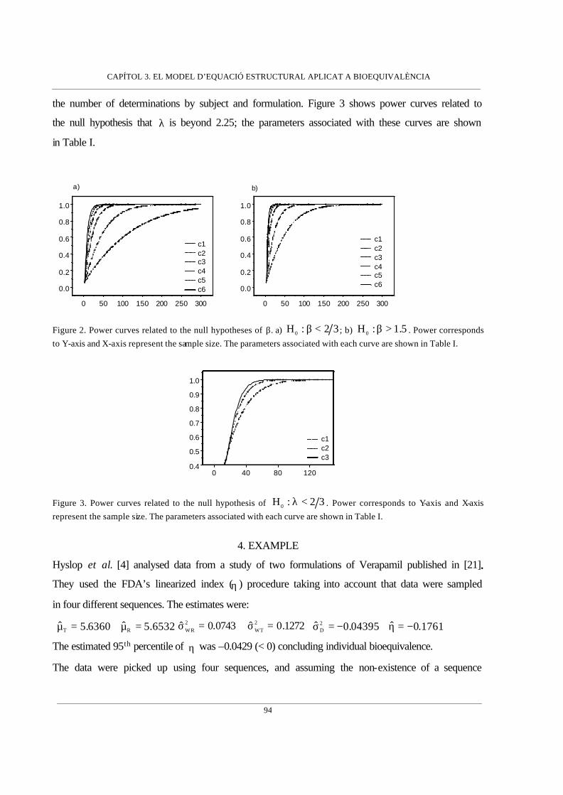
CAPÍTOL 3. EL MODEL D’EQUACIÓ ESTRUCTURAL APLICAT A BIOEQUIVALÈNCIA
94
the number of determinations by subject and formulation. Figure 3 shows power curves related to
the null hypothesis that λ is beyond 2.25; the parameters associated with these curves are shown
in Table I.
0 50 100 150 200 250 300
0.0
0.2
0.4
0.6
0.8
1.0
c1c2c3c4c5c6
a)
0 50 100 150 200 250 300
0.0
0.2
0.4
0.6
0.8
1.0
c1c2c3c4c5c6
b)
Figure 2. Power curves related to the null hypotheses of β. a) 32:H0 <β ; b) 5.1:H0 >β . Power corresponds to Y-axis and X-axis represent the sample size. The parameters associated with each curve are shown in Table I.
0 40 80 1200.4
0.5
0.6
0.7
0.8
0.9
1.0
c1c2c3
Figure 3. Power curves related to the null hypothesis of 32:H0 <λ . Power corresponds to Y-axis and X-axis represent the sample size. The parameters associated with each curve are shown in Table I.
4. EXAMPLE
Hyslop et al. [4] analysed data from a study of two formulations of Verapamil published in [21].
They used the FDA’s linearized index (η ) procedure taking into account that data were sampled
in four different sequences. The estimates were:
6532.5ˆ6360.5ˆ RT =µ=µ 1272.0ˆ0743.0ˆ 2WT
2WR =σ=σ 1761.0ˆ04395.0ˆ 2
D −=η−=σ
The estimated 95th percentile of η was –0.0429 (< 0) concluding individual bioequivalence.
The data were picked up using four sequences, and assuming the non-existence of a sequence

CAPÍTOL 3. EL MODEL D’EQUACIÓ ESTRUCTURAL APLICAT A BIOEQUIVALÈNCIA
95
effect we proceed by joining all subjects in a unique sequence with two measurements by
formulation and subject. The individual means estimate were provided by:
∑∑==
+==2
1j
ijRi
2
1j
iji e21
uR21
R and ∑∑==
+==2
1j
ijTi
2
1j
iji e21
uT21
T . Applying the methods
described in section 3.2, the SEM estimates obtained were:
( ) 1789.1ˆ.E.S7304.0ˆ
=α=α
( ) 2074.0ˆ.E.S
8646.0ˆ
=β
=β
2472.0ˆ
6661.5ˆ2BR
R
=σ
=µ
( ) 0926.0ˆ.E.S036.0ˆ=ϕ
−=ϕ
4146.1ˆ1290.0ˆ0912.0ˆ 2WT
2WR =λ=σ=σ
and using these estimated parameters we can proceed with the hypotheses tests associated with
individual bioequivalence.
1. Hypothesis concerning β . The bioequivalent limits for β are [ ]5.1,32 . The 90% confidence
interval for β is [0.5084 , 1.2208] which has a lower limit lower than the bioequivalent limit,
so we don’t reject the no-bioequivalence hypothesis of β < 2/3.
2. Hypothesis concerning ϕ . The bioequivalent limits for ϕ are
[ ] [ ]2231.0 , 2231.025.1ln,25.1ln −≈⋅− . The 90% confidence interval for ϕ is
[ ]1225.0 , 1961.0− which is completely inside the bioequivalent interval, thus we reject the
null hypothesis about ϕ .
3. Hypothesis concerning within-subject variances. The estimate of the ratio of within-subjects
variances is 4146.1ˆˆˆ 2WR
2WT =σσ=λ . The 95th percentile of F distribution with 23 and 23
degrees of freedom is 2.014, and so the 95th percentile of λ is 2.8495, greater than 2.25. Thus,
we don’t reject the null hypothesis concerning λ.
Therefore, the decision is no-bioequivalence due to β and to λ. Table II shows the power of each
hypothesis under two alternative hypotheses: parameters are equal to their estimate and
parameters are those defined by perfect individual bioequivalence. We have also estimated the
power with a sample size of 50 and 100 subjects. From the results it seems that a number of
subjects between 50 and 100 would yield a reasonable power to take a decision.
Disagreement between the FDA index and the SEM approach in this case could be explained
through the lack of power of the SEM approach. However, the greater power of the FDA
approach might be due to aggregation of bioequivalent limits. The FDA index limit is based on
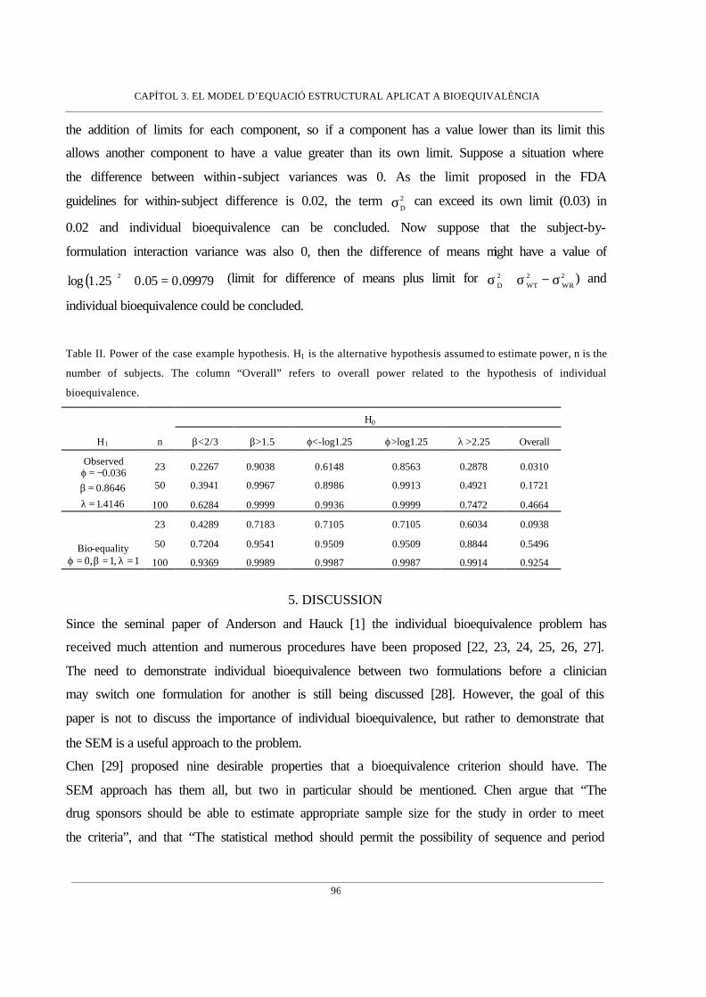
CAPÍTOL 3. EL MODEL D’EQUACIÓ ESTRUCTURAL APLICAT A BIOEQUIVALÈNCIA
96
the addition of limits for each component, so if a component has a value lower than its limit this
allows another component to have a value greater than its own limit. Suppose a situation where
the difference between within-subject variances was 0. As the limit proposed in the FDA
guidelines for within-subject difference is 0.02, the term 2Dσ can exceed its own limit (0.03) in
0.02 and individual bioequivalence can be concluded. Now suppose that the subject-by-
formulation interaction variance was also 0, then the difference of means might have a value of
( ) 09979.005.025.1log 2 =+ (limit for difference of means plus limit for 2WR
2WT
2D σ−σ+σ ) and
individual bioequivalence could be concluded.
Table II. Power of the case example hypothesis. H1 is the alternative hypothesis assumed to estimate power, n is the
number of subjects. The column “Overall” refers to overall power related to the hypothesis of individual
bioequivalence.
H0
H1 n β<2/3 β>1.5 ϕ<-log1.25 ϕ>log1.25 λ >2.25 Overall
23 0.2267 0.9038 0.6148 0.8563 0.2878 0.0310
50 0.3941 0.9967 0.8986 0.9913 0.4921 0.1721
Observed
4146.1
8646.0036.0
=λ=β
−=ϕ
100 0.6284 0.9999 0.9936 0.9999 0.7472 0.4664
23 0.4289 0.7183 0.7105 0.7105 0.6034 0.0938
50 0.7204 0.9541 0.9509 0.9509 0.8844 0.5496 Bio-equality 1,1,0 =λ=β=ϕ 100 0.9369 0.9989 0.9987 0.9987 0.9914 0.9254
5. DISCUSSION
Since the seminal paper of Anderson and Hauck [1] the individual bioequivalence problem has
received much attention and numerous procedures have been proposed [22, 23, 24, 25, 26, 27].
The need to demonstrate individual bioequivalence between two formulations before a clinician
may switch one formulation for another is still being discussed [28]. However, the goal of this
paper is not to discuss the importance of individual bioequivalence, but rather to demonstrate that
the SEM is a useful approach to the problem.
Chen [29] proposed nine desirable properties that a bioequivalence criterion should have. The
SEM approach has them all, but two in particular should be mentioned. Chen argue that “The
drug sponsors should be able to estimate appropriate sample size for the study in order to meet
the criteria”, and that “The statistical method should permit the possibility of sequence and period

CAPÍTOL 3. EL MODEL D’EQUACIÓ ESTRUCTURAL APLICAT A BIOEQUIVALÈNCIA
97
effect, as well as missing data”. Sample size estimation is a question that has been tackled
through the power analysis. Potential users of the SEM approach should pay attention to the
magnitude of within-subjects variances and, above all, to signal-to-noise of both formulations.
The power of he hypothesis concerning λ can be increased by taking more determinations by
subject and formulation, whereas a higher signal-to-noise would yield a better power for β . The
way to increase signal-to-noise is through increasing the between-subjects variance of reference
method and this means collecting subjects with a greater spread of data. In fact, a larger signal-to-
noise of reference method will generate a higher power and also avoid the Gleser-Hwang effect.
With respect to sample size, the power analysis indicates that the FDA’s suggestion of a
minimum number of 12 subjects [2] is quite inadequate for SEM analysis, where a sample size
between 50 and 100 subjects would be more satisfactory in terms of power.
In relation to sequence effect, even though the SEM procedure might easily model this effect
including a covariate [8], we believe that in the context of a bioequivalence study the absence of
sequence effect is a measurement model assumption, like normal distribution or linearity of the
effects, and we should be reasonably convinced about the non-existence of this effect.
In this paper, we have assumed both formulations were replicated and both within-subject
variances were estimated from these replicates, but what would happen if only one formulation
was replicated? In this case, we would only be able to estimate one of the within-subject
variances from the replicates, but nevertheless, the model would be identified and estimation
could still be carried out. The formulae of estimates and standard errors would, however, be
different [8].
SEM is a disaggregate procedure because it evaluates separately each component of the model
related to individual bioequivalence, whereas the FDA index is an aggregate approach. Some
authors have argued in favour of disaggregate as opposed to an aggregate approach [30, 31, 32,
33]. The most important criticism against the aggregate procedure in questions of individual
bioequivalence is the trade-off among components, namely, the trade-off between average and
within-subject components and, specifically, that within-subject variance of tested formulation is
greater than within-subject variance of reference formulation ( 2WR
2WT σ<σ ). The FDA Individual
Bioequivalence Working Group took this matter into account and proposed some solutions [34],
such as weighting the FDA index components in order to avoid the trade-off. However, the
question is not only the trade-off when 2WR
2WT σ<σ , but when any component has a value lower

CAPÍTOL 3. EL MODEL D’EQUACIÓ ESTRUCTURAL APLICAT A BIOEQUIVALÈNCIA
98
than its bioequivalent limit, as has been shown in the case example. This “limit trade-off” could
lead to a bizarre situation where individual bioequivalence is achieved but average
bioequivalence isn’t. The root of this problem lies in the fact that the bioequivalent limit for the
aggregate index is obtained by combining disaggregated limits for each component. In our view,
a disaggregated criterion is more consistent and appropriate for bioequivalent limits derived in a
disaggregate way such as those proposed by the FDA.
A disaggregate criterion has been criticized because it can produce multiplicity problems through
combining different hypotheses and the need to specify multiple limits [35]. Since the
intersection-union principle has been used in the present study, the multiplicity problem is
avoided; as for the multiple limits, the limit for the aggregate criterion is established by adding
multiple limits so no extra complexity results from using multiple acceptance limits in a
disaggregate approach.
Summing up, it was demonstrated that SEM is a useful approach to the individual bioequivalence
problem. The fact that SEM is a disaggregate approach has two advantages. Firstly, it enables the
sources of no-bioequivalence to be easily found; and secondly, the aggregation of the
bioequivalent limits is avoided. An additional advantage could be that because SEM is a
regression procedure it is more straightforward approach for potential users.
ACKNOWLEDGMENTS
We thank to Dr. A. Cobos for his criticism on an earlier draft of this work. We are also grateful
to two anonymous referees who made helpful comments on the manuscript. Robin Rycroft from
SAL (Universitat de Barcelona) improved the English text.
REFERENCES
1. Anderson S., Hauck WW. Consideration of individual bioequivalence. Journal of Pharmacokinetics and
Biopharmaceutics 1990; 18: 259-274
2. U.S. Department of Health and Human Services, Food and Drug Administration , Center for
Drug Evaluation and Research (CDER). Guidance for Industry. Statistical Approaches to
Establishing Equivalence. CDER, 2001
3. Schall R, Luus HG. On population and individual bioequivalence. Statistics in Medicine 1993; 12: 1109-1124.
4. Hyslop T, Hsuan F, Holder DJ. A small sample confidence interval approach to assess individual bioequivalence.
Statistics in Medicine 2000; 19: 2885-2897
CAPÍTOL 3. EL MODEL D’EQUACIÓ ESTRUCTURAL APLICAT A BIOEQUIVALÈNCIA
99
5. Kelly GE. Use of the structural equations model in assessing the reliability of a new
measurement technique. Applied Statistics 1985; 34(3):258-263
6. Tan CY and Iglewicz B. Measurement-methods comparisons and linear statistical relationship.
Technometrics 1999, 41(3): 192-201
7. Dragalin V and Fedorov V. The total least squares method in individual bioequivalence
evaluation. Biometrical Journal 2001, 43(4): 399-420
8. Cheng CL, van Ness JW. Statistical Regression with Measurement Error. Kendall’s Library of Statistics. Arnold:
London, 1999
9. Cox DR. Partial likelihood. Biometrika 1975; 62: 269-276
10. Chinchilli VM, Esinhart JD and Miller WG. Partial likelihood analysis of within-unit variances in repeated
measurement experiments. Biometrics 1995; 51(1): 205-216.
11. Birch MW. A note on the maximum likelihood estimation of a linear structural relationship. Journal of the
American Statistical Association 1964; 59: 1175-1178
12. Gleser LJ. A note on G.R. Dolby’s unreplicated ultrastructural model. Biometrika 1985, 72:
117-124.
13. Fuller WA. Measurement error models. John Wiley & Sons: New York. 1987.
14. Lehman EL. Testing statistical hypotheses, second edition. John Wiley & Sons: New York.
1986.
15. Roy SN. On a heuristic method of test construction and its use in multivariate analysis.
Annals of Mathematical Statistics 1953; 24: 220-238
16. Wellek, S. On a reasonable disaggregate criterion of population bioequivalence admitting of resampling-free
testing procedures. Statistics in Medicine 2000; 19: 2755-2767
17. Schuirmann DJ. A comparison of the two one-sided test procedure and the power approach
for assessing the equivalence of average bioavailability. Journal of Pharmacokinetics and
Biopharmaceutics 1987; 15: 657-680.
18. Gleser LJ. Confidence intervals for the slope in a linear errors-in-variables regression model.
In Advances in Multivariate Statistical Analysis 1987. Ed. K. Gupta. D. Reidel: Dordrecht. 85-
109
19. Gleser LJ and Hwang JT. The non-existence of 100(1-α)% confidence sets of finite expected
diameter in errors-in-variables and related models. The Annals of Statistics 1987, 15: 1351-1362.
20. Berger RL, Hsu JC. Bioequivalence trials, intersection-union tests and equivalence
confidence sets. Statistical Science 1996; 11(4): 283-319
CAPÍTOL 3. EL MODEL D’EQUACIÓ ESTRUCTURAL APLICAT A BIOEQUIVALÈNCIA
100
21. Chinchilli VM. The Assessment of individual and population bioequivalence. Journal of Biopharmaceutical
Statistics 1996. 6: 1-14
22. Sheiner LB. Bioequivalence revisited. Statistics in Medicine 1992; 11: 1777-1788
23. Holder DJ, Hsuan F. Moment-based criteria for determining bioequivalence. Biometrika 1993; 80(4): 835-846
24. Esinhart JD, Chinchilli VM. Extension to the use of tolerance intervals for the assessment of individual
bioequivalence. Journal of the Biopharmaceutical Statistics 1994; 4(1): 39-52
25. Vuorinen J, Turunen J. A three-step procedure for assessing bioequivalence in the general mixed model
framework. Statistics in Medicine 1996; 15(24): 2635-2655
26. Gould AL. A practical approach for evaluating population and individual bioequivalence. Statistics in Medicine
2000; 19(20): 2721-2740
27. Lin LI. Total deviation index for measuring individual agreement with applications in laboratory performance
and bioequivalence. Statistics in Medicine 2000; 19: 255-270
28. Senn S. Statistical issues in bioequivalence. Statistics in Medicine 2001; 20: 2785-2799
29. Chen ML. Individual bioequivalence – A regulatory update. Journal of Biopharmaceutical Statistics 1997; 7(1):
5-11
30. Liu JP, Chow SC. Some thoughts on individual bioequivalence. Journal of
Biopharmaceutical Statistics 1997; 7(1): 41-48.
31. Vuorinen J. A practical approach for the assessment of bioequivalence under selected higher-
order cross-over designs. Statistics in Medicine 1997; 16: 2229-2243
32. Hauschke D, Steinijans VW. The U.S. draft guidance regarding population and individual
bioequivalence approaches: comments by a research-based pharmaceutical company. Statistics in
Medicine 2000; 19: 2769-2774
33. Endrenyi L, Hao Y. Asymmetry of the mean-variability tradeoff raises questions about the
model in investigations of individual bioequivalence. International Journal of Clinical
Pharmacology and Therapeutics 1998; 36(8): 450-457.
34. Hauck WW, Chen ML, Hyslop T, Patnaik R, Schuirmann D and Williams R. Mean
difference vs. variability reduction: tradeoffs in aggregate measures for individual
bioequivalence. International Journal of Clinical Pharmacology and Therapeutics 1996; 34(12):
535-541.
35. Chen ML, Patnaik R, Hauck WW, Schuirmann DJ, Hyslop T and Williams R. An individual
bioequivalence criterion: regulatory considerations. Statistics in Medicine 2000; 19: 2821-2842
CAPÍTOL 3. EL MODEL D’EQUACIÓ ESTRUCTURAL APLICAT A BIOEQUIVALÈNCIA
101
The structural error-in-equation model to evaluate individual
bioequivalence
Josep L. Carrasco and Lluís Jover
Bioestadística, Departament de Salut Pública. Universitat de Barcelona, Barcelona, Spain
ABSTRACT
Individual bioequivalence is assessed using an extension of the classical structural equation model, known as the
error-in-equation model. This procedure estimates the relationship between individual means, as well as the
variance-covariance parameters, of the bioavailabilities measurement model, by considering individual means related
through a straight line with a random term, whereas the classical structural equation considers a deterministic linear
relationship. We discuss the implications of this approach in terms of the bioavailabilities measurement model and
how to test the overall hypothesis of individual bioequivalence. Both models are compared in a simulation study and
a case examp le is presented.
KEY WORDS: Individual bioequivalence, structural equation model, structural error-in-equation model, union-
intersection principle
1. INTRODUCTION
Two formulations are considered bioequivalent if they have the same amount of bioavailabilit ies.
If this condition holds, they can then be assumed to have the same therapeutic effect (1).
Bioavailabilites are measured using a pharmacokinetic curve, where the area under the curve
(AUC), the maximum concentration (Cmax) and the time to reach the maximum concentration
(Tmax) are the most frequently used measures.
If the bioavailabilites are measured from n individuals k times, it is assumed that taking
logarithms on bioavailabilities the underlying measurement model is (2):
RijRiij
TijTiij
euR
euT
+=
+=
where Tij and Rij are the log-bioavailabilities of tested and reference formulations respectively, µT
and µR are the overall averages of T and R, uTi and uRi are the mean deviations from the overall
averages of individual i, and eTij and eRij are the random deviations of i individual on j

CAPÍTOL 3. EL MODEL D’EQUACIÓ ESTRUCTURAL APLICAT A BIOEQUIVALÈNCIA
102
determination, with i=1,..,n and j=1,...,k. It is assumed that ( )BTTiT ,N~u σµ , ( )BRRRi ,N~u σµ ,
( )WTTij ,0N~e σ and ( )WRRij ,0N~e σ .
Formerly bioequivalence was assayed by comparing the overall means of the bioavailabilites (3)
and if the difference between µT and µR was sufficiently small then bioequivalence was accepted.
However, Anderson and Hauck (4) demonstrated that this equality was insufficient to guarantee
switchability between formulations and defined bioequivalence as “average bioequivalence”.
They then proposed two new bioequivalence concepts: population bioequivalence and individual
bioequivalence.
Population bioequivalence is achieved if it can be demonstrated that the bioavailabilites of both
formulations are from the same probability distribution. Since a normal distribution is assumed
for bioavailabilites, populational bioequivalence is reduced to demonstrate equality of averages
plus equality of overall variances, a concept that can be associated with the prescribability of a
new formulation.
Individual bioequivalence requires equality of each individual’s bioavailabilites, and hence
operates with a probability distribution that is conditioned to the individual rather than the
population distribution. In this case, individual bioequivalence requires equality between the
overall averages, µT and µR , between the individual mean deviations, uRi and uTi, and between
the variances of the within-subjects variances 2WRσ and 2
WTσ . Thus, true individual
bioequivalence requires perfect agreement among the bioavailabilities of each individual.
However, this criterion is usually relaxed so that it is sufficient for declaring individual
bioequivalence if the differences are within certain limits, known as the limits of bioequivalence.
The criterion proposed by the Food and Drug Administration (5) is an aggregate index which
includes all the terms involved in individual bioequivalence. Here it is not our intention to discuss
this criterion but rather we wish to use the structural error-in-equation model (SEEM), an
extension of the structural equation model (SEM) presented by Carrasco and Jover (6), in order to
assess individual bioequivalence.
CAPÍTOL 3. EL MODEL D’EQUACIÓ ESTRUCTURAL APLICAT A BIOEQUIVALÈNCIA
103
2. THE MODEL
2.1 Structural Equation Model
The structural equation model assumes that the relationship between the individual means is a
straight line RiTi uu ⋅β+α= . This structural equation implies that the average of the tested
formulation is RT µ⋅β+α=µ , the between-subjects variance of tested formulation is
2BR
22BT σβ=σ and the covariance between tested and reference formulations is equal to
2BRRT σ⋅β=σ . The difference in overall means can be expressed as ( ) RRT 1 µ⋅−β+α=µ−µ=ϕ .
Bioequality can be said to hold when there is equality of means, equality of between-subjects
variances and equality between within-subjects variances. Because BRBT σσ=β and
2WR
2WT σσ=λ , individual bioequivalence can be assessed by evaluating ϕ , β and λ separately.
Individual bioequivalence can then be established if ϕ , β and λ lie within the respective limits
of bioequivalence.
Drawing on FDA guidelines for establishing bioequivalence limits, Carrasco and Jover (6)
proposed using: 25.1ln±∈ϕ for difference of means, which comes from the criterion for
average bioequivalence; [ ]5.1,32
BRBT ∈σσ for between-subjects variances, whereby any of the
between-subjects standard deviations can exceed the other one 1.5 times; and finally,
25.22WR
2WT ≤σσ , whereby the within-subject standard deviation of tested formulation cannot
exceed the within-subject standard deviation of the reference formulation more than 2.25 times
The overall null hypothesis of no-individidual bioequivalence can be evaluated testing the
following five hypotheses
32:H
32:H
11
01
≥β
<β
5.1:H
5.1:H
12
02
≤β
>β
25.1ln:H
25.1ln:H
13
03
−≥ϕ
−<ϕ
25.1ln:H
25.1ln:H
14
04
≤ϕ
>ϕ
25.2:H
25.2:H
15
05
≤λ
>λ
The overall hypothesis in relation to individual bioequivalence is expressed as
H0: No-bioequivalence = 0504030201 HHHHH ∪∪∪∪
HA: Bioequivalence = 1514131211 HHHHH ∩∩∩∩

CAPÍTOL 3. EL MODEL D’EQUACIÓ ESTRUCTURAL APLICAT A BIOEQUIVALÈNCIA
104
A mixed hypothesis of this type can be tested using Roy’s intersection-union principle (7).
Applying this principle, the null hypothesis of no-bioequivalence is rejected at level α if all null
hypotheses are rejected at level α .
2.2 Structural Error-in-Equation Model
This model fits the underlying measurement model introducing an error term in the structural
equation iRiTi quu +⋅β+α= assuming ( )qi ,0N~q σ (8). This term signifies that the relationship
between individual means can vary from one individual to another, then RiTi uu ⋅β+α= denotes
an average relationship. In fact, SEEM is no more than a simple regression model between two
unobservable variables.
Therefore, we are concerned with a new term in the individual bioequivalence assay: the variance
of the equation error. In claiming individual bioequivalence not only must the structural equation
be reasonably close to the concordance line (α = 0 and β = 1), but the pair of points ( )TiRi u,u has
to lie near the straight line, so 2qσ must be small.
The hypotheses concerning overall means and the within-subjects variance ratio remain the same.
In relation to 2qσ we have to be assured that the pair of individual means lies near the line. In this
order, we propose using a correlation coefficient between uRi and uTi rather than 2qσ . In this case,
the expression of this coefficient in terms of the model is:
( )( ) ( ) ( ) 2
q2BR
2
BR
2q
2BR
22BR
2BR
2BT
2BR
RT
TR
TR
uVaruVaru,ucov
σ+σ⋅βσ⋅β
=σ+σ⋅β⋅σ
σ⋅β=
σ⋅σσ
=⋅
=ρ .
consequently a lower limit for this coefficient has to be set to establish individual bioequivalence.
Our proposal is a correlation coefficient of 0.9. This limit is set intuitively as we understand a
value of 0.9 to be a high value, however, another limit might be used were it necessary to vary
the restrictive nature of the criterion.
Finally, the ratio of between-subjects variances is
2
2
2BR
2q
2BR
2
2BR
2BT
ρβ
=σ
σ+σ⋅β=
σσ ,
which means that the tolerance concerning the value of β depends on the correlation between uTi
and uRi.

CAPÍTOL 3. EL MODEL D’EQUACIÓ ESTRUCTURAL APLICAT A BIOEQUIVALÈNCIA
105
Therefore, when using SEEM it is necessary to evaluate six hypotheses to assess individual
bioequivalence:
32:H
32:H
11
01
≥ρβ
<ρβ
5.1:H
5.1:H
12
02
≤ρβ
>ρβ
25.1ln:H
25.1ln:H
13
03
−≥ϕ
−<ϕ
25.1ln:H
25.1ln:H
14
04
≤ϕ
>ϕ
25.2:H
25.2:H
15
05
≤λ
>λ and
9.0:H
9.0:H
16
06
≥ρ
<ρ
3. INFERENCE
3.1 Maximum Likelihood Estimates
Structural models usually have problems identifying the model. This means that there is not
sufficient information in the data to produce maximum likelihood estimates. In such a situation,
extra information, such as the knowledge of the value of a parameter, is required. This extra
information can be derived from others assays or by taking replicates in the same assay. These
replicates can then be used to estimate the within-subject variances, which become the identified
model. The SEM introduced need only replicate one of the two formulations to obtain an
identifiable model, whereas the SEEM needs to replicate both formulations. Here, we will
consider both formulations replicated k times over each subject with k greater than one.
Chinchilli et al. (9) proposed a partial likelihood analysis in which the full likelihood was
separate in a conditional likelihood depending on within-subject variances and individual means
plus a marginal likelihood based on within-subject variances.
( ) ( ) ( )2T
2R
2WT
2WR2ii
2WT
2WR2|1ijij
2WT
2WR W,W,,LT,R,,|LT,R,,,L σσ+σσθ=σσθ
where
*RijRi
k
1jRijRi
k
1jiji eue
k1
uRk1
R +=+== ∑∑==
( )∑∑= =
−=n
1i
k
1j
2
iij2
R RRW
*TijTi
k
1jTijTi
k
1jiji eue
k1
uTk1
T +=+== ∑∑==
, ( )∑∑= =
−=n
1i
k
1j
2
iij2
T TTW
L2 is used to obtain the maximum likelihood estimates of the within-subject variances
( ) ( ) ( ) ( )2WT
2WR
n
1i
k
1j
n
1i
k
1j
2
iij2WT
2
iij2WR ˆ
ˆˆTT1kn
1ˆRR1kn
1ˆσσ
=λ−−⋅
=σ−−⋅
=σ ∑∑ ∑∑= = = =
CAPÍTOL 3. EL MODEL D’EQUACIÓ ESTRUCTURAL APLICAT A BIOEQUIVALÈNCIA
106
where k is the number of replicates, n the number of subjects and θ the remaining parameters of
the model. The θ maximum likelihood estimates are achieved maximizing L1, which is
equivalent to maximizing the likelihood of a common structural model with no replicates with
iR and iT as data and with the knowledge of within-subjects as extra information.
In the case of a simple structural model with no error in the equation, the estimates for θ are
obtained considering a model where both within-subject variances are known (6, 8), but when
there is an error in the equation, the estimate changes because the random error of the tested
formulation cannot be considered as known. This can be easily demonstrated by developing iT in
terms of the structural equation:
TijRi*TijiRi
*TijTii uequeuT ε+⋅β+α=++⋅β+α=+= .
The random term Tijε comprises both the attenuated within-subject variation and the error of the
equation. In this case, the estimation is carried out by considering just the within-subject variance
of the known reference formulation with the maximum likelihood estimates (8)
kˆS
Sˆ2WR2
R
RT
σ−=β ( ) RX1ˆˆˆ ⋅−β+α=ϕ
RT XˆXˆ ⋅β−=α k
ˆSˆ2WR2
R2BR
σ−=σ k
ˆSˆSˆ2WT
RT2T
2q
σ−⋅β−=σ
provided that kS2WR2
Rσ> and
σ−≥ kSSS
2WR2
R2RT
2T
, where RT
2T
2RTR S,S,S,X,X are the
sample means, variances and covariance of iR and
iT , respectively.
Cheng and van Ness (10) proved that ( )β−βα−α ˆ,ˆn 21 has an asymptotically jointly normal
distribution with 0 vector mean and covariance matrix equal to
( )
ψψ⋅µ−
ψ⋅µ−ψ⋅µ+θ=βαΣ
11R
1R12Rˆ,ˆ ,
where
σβ+
σ+σθ⋅σ=ψ −
22WR2
2WR2
BR4
BR1 kk and ( )2
WR22
WTk1
σβ+σ=θ .
The standard error of the difference of means ϕ is given by ( )( )Rˆ1ˆˆVar µ⋅−β+α which in is
equal to nθ .
CAPÍTOL 3. EL MODEL D’EQUACIÓ ESTRUCTURAL APLICAT A BIOEQUIVALÈNCIA
107
3.2 Hypotheses Testing
In this section we explain how to evaluate the hypotheses concerning the SEEM parameters,
when an error is assumed in the equation. We address the reader to (6) for a similar discussion of
the evaluation of hypotheses concerning the SEM.
3.2.1 Difference of Means
The hypothesis concerning difference of means, ϕ , will be tested in a two one-sided way, then
both null hypotheses will be rejected at level α if the ( )%21 α− confidence interval lies within
the bioequivalent interval. The confidence interval concerning ϕ can be estimated using the
property of asymptotic normality, whereas (11) suggests using a t-student distribution in small
samples, therefore a t-student distribution with 2n − degrees of freedom will be used.
3.2.2 Ratio of between-subject standard deviation
To test the hypotheses concerning the ratio ρβ we rewrite the hypotheses as
032:H 101 <ρ−β=η
and
05.1:H 202 >ρ−β=η .
To test this sort of hypothesis we will estimate the α% percentile of 1η and the ( )%1 α−
percentile of 2η rejecting the hypotheses if 0ˆ %,1 >η α and 0ˆ %1,2 <η α− respectively. These
percentiles can be approximated using a procedure based on a Cornish-Fisher expansion (12).
Following this procedure we can approximate the α% percentile of ρ⋅θ+β=η ˆˆˆ as
( ) ( ) 21
VVsignˆ ⋅+η where ( ) ( ) ( ) ( ){ }ρ−ρ⋅ρ−ρ⋅θ+β−β⋅β−β= αααα ˆˆˆˆˆˆˆˆV 2 , indicating αβ and
αρ
the α% percentile of β and ρ respectively.
The α% percentile of β can be estimated using a t-student distribution with n-1 degrees of
freedom (11) whereas the α% percentile of ρ is estimated according to whether the percentile is
greater or lower than the median. If α>50% the percentile is estimated as
( ) ( )( ) ( ) ρ⋅−++
−+ρ⋅+
αα
αα
ˆF1F1F1ˆF1

CAPÍTOL 3. EL MODEL D’EQUACIÓ ESTRUCTURAL APLICAT A BIOEQUIVALÈNCIA
108
whereas if α<50% the expression is
( ) ( )( ) ( ) ρ⋅−−+
−−ρ⋅+
αα
αα
ˆF1F1F1ˆF1
where Fα is the α% percentile of an F-distribution with n-2 and n-2 degrees of freedom (13).
3.2.3 Ratio of within-subject variances
Assuming within-subject variabilities are normally distributed, both within-subjects variances
follow chi-square distributions with ( )1kn −⋅ degrees of freedom (9). Therefore the within-
subjects variance ratio follows an F-distribution with ( )1kn −⋅ and ( )1kn −⋅ degrees of freedom.
So the hypothesis concerning within-subjects variances can be tested by estimating the ( )%1 α−
percentile of λ , where α is the significance level desired. This percentile is estimated as
21 ,,1Fˆννα−⋅λ , where
21 ,,1F ννα− is the ( )%1 α− percentile of an F-distribution with ( )1kn21 −⋅=ν=ν
degrees of freedom, where k is the number of measures by subject and formulation. The
hypothesis will be rejected if 25.2Fˆ21 ,,1 <⋅λ ννα−
3.2.4 Correlation coefficient between individual means
The hypothesis concerning the correlation coefficient between uT and uR 9.0:H 0 <ρ can be
evaluated by estimating the α% percentile of ρ , where α is the significance desired. This
percentile is estimated using the procedure explained in section 3.2.2. The null hypothesis is
rejected if 9.0ˆ % >ρα .
3.3 Model selection
The SEEM seems to be a better way to model the log-bioavailabilities measurement model than
the SEM because the SEM is no more than a particular case of SEEM, but it is possible that the
relationship between the individuals means will be the same for all individuals, in which case the
equation should not contain an error term and the SEM would be preferable. Thus, a procedure
for deciding between both models is required.

CAPÍTOL 3. EL MODEL D’EQUACIÓ ESTRUCTURAL APLICAT A BIOEQUIVALÈNCIA
109
The first step in deciding between both models is related to the value of 2qσ , because in fact the
maximum likelihood estimation of 2qσ is { }2
qˆ,0max σ , but it is possible to find a negative estimate
of 2qσ . In this case the value of 2
qσ must be set to 0 an estimate the model again, which means
using the SEM. So, a negative value of 2qσ is a criterion for deciding between the SEM and the
SEEM.
If 2qσ has a positive value, the likelihood ratio test (LRT) (14) can be used. This test is based on
the log-likelihood of the structural model:
( ){ }pSlogStracelog2n
L 1 −−Σ+Σ−∝ − ,
where p is the number of variables (in our case p=2), Σ is the covariance matrix between iR and
iT based on the model and S is the sample covariance matrix between iR and
iT , which means
in the case of SEM
σ+σβσβ
σβσ+σ=Σ
kˆˆˆˆˆ
ˆˆk
ˆˆ
21,WT2
1,BR21
21,BR1
21,BR1
21,WR2
1,BR
1,
whereas in the case of SEEM
σ+σ+σβσβ
σβσ+σ=Σ
kˆˆˆˆˆˆ
ˆˆk
ˆˆ2
2,WT2q
22,BR
22
22,BR2
22,BR2
22,WR2
2,BR
2.
Therefore, we can define L1 and L2, and under the null hypothesis of 0ˆ 2q =σ the quantity
( )12 LL2 −⋅ is distributed under a chi-square distribution with 1 degree of freedom.
4. SIMULATION STUDY
In order to compare the behaviour of both the SEM and the SEEM in different situations, a
simulation study was carried out. We simulated nine combinations of the measurement model
parameters (Table I). All the combinations maintained a difference of means of 0 and a ratio of
within subject variances of 1. Only the slope of the equation (β) and the correlation between
individual means (ρ) varied producing non individual bioequivalence situations in combinations
3, 6 and 9. We took a thousand samples of each parameter combination and we evaluated the
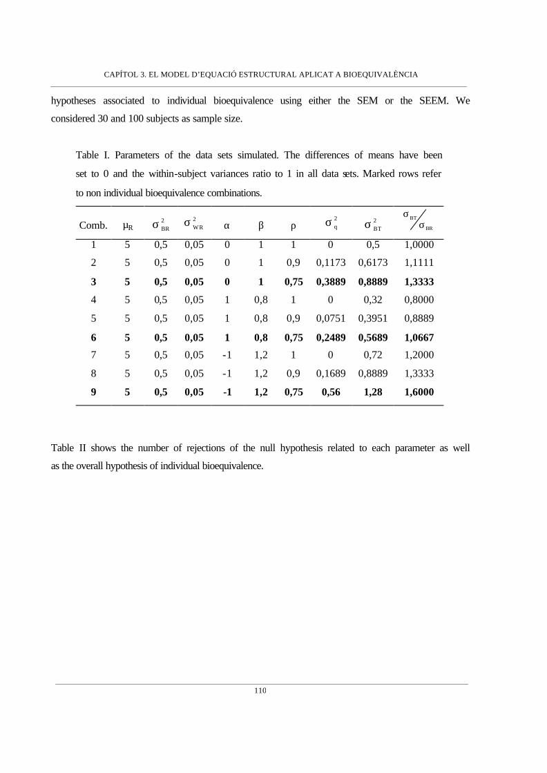
CAPÍTOL 3. EL MODEL D’EQUACIÓ ESTRUCTURAL APLICAT A BIOEQUIVALÈNCIA
110
hypotheses associated to individual bioequivalence using either the SEM or the SEEM. We
considered 30 and 100 subjects as sample size.
Table I. Parameters of the data sets simulated. The differences of means have been
set to 0 and the within-subject variances ratio to 1 in all data sets. Marked rows refer
to non individual bioequivalence combinations.
Comb. µR 2BRσ
2WRσ α β ρ
2qσ 2
BTσ BR
BT
σσ
1 5 0,5 0,05 0 1 1 0 0,5 1,0000
2 5 0,5 0,05 0 1 0,9 0,1173 0,6173 1,1111
3 5 0,5 0,05 0 1 0,75 0,3889 0,8889 1,3333
4 5 0,5 0,05 1 0,8 1 0 0,32 0,8000
5 5 0,5 0,05 1 0,8 0,9 0,0751 0,3951 0,8889
6 5 0,5 0,05 1 0,8 0,75 0,2489 0,5689 1,0667
7 5 0,5 0,05 -1 1,2 1 0 0,72 1,2000
8 5 0,5 0,05 -1 1,2 0,9 0,1689 0,8889 1,3333
9 5 0,5 0,05 -1 1,2 0,75 0,56 1,28 1,6000
Table II shows the number of rejections of the null hypothesis related to each parameter as well
as the overall hypothesis of individual bioequivalence.
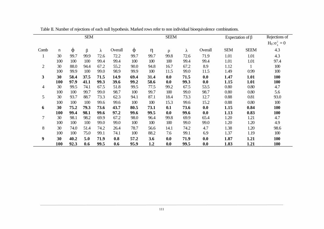
111
Table II. Number of rejections of each null hypothesis. Marked rows refer to non individual bioequivalence combinations.
SEM SEEM Expectation of β Rejections of H0: 02
q =σ
Comb n ϕ β λ Overall ϕ η ρ λ Overall SEM SEEM 4.3 30 99.7 99.9 72.6 72.2 99.7 99.7 99.8 72.6 71.9 1.01 1.01 4.3 1 100 100 100 99.4 99.4 100 100 100 99.4 99.4 1.01 1.01 97.4 30 88.0 94.4 67.2 55.2 90.0 94.8 16.7 67.2 8.9 1.12 1 100 2 100 99.9 100 99.0 98.9 99.9 100 11.5 99.0 11.5 1.49 0.99 100 30 58.4 37.5 71.5 14.9 69.4 31.4 0.0 71.5 0.0 1.47 1.01 100 3
100 97.9 41.1 99.3 39.6 99.2 58.6 0.0 99.3 0.0 1.15 1.01 100 30 99.5 74.1 67.5 51.8 99.5 77.5 99.2 67.5 53.5 0.80 0.80 4.7 4 100 100 99.7 99.0 98.7 100 99.7 100 99.0 98.7 0.80 0.80 5.6 30 93.7 88.7 73.3 62.3 94.1 87.1 18.4 73.3 12.7 0.88 0.81 93.0 5 100 100 100 99.6 99.6 100 100 15.3 99.6 15.2 0.88 0.80 100 30 75.2 79.3 73.6 43.7 80.5 73.1 0.1 73.6 0.0 1.15 0.84 100 6
100 99.4 98.1 99.6 97.2 99.6 99.5 0.0 99.6 0.0 1.13 0.83 100 30 98.1 98.2 69.9 67.2 98.0 96.4 99.8 69.9 65.4 1.20 1.21 4.7 7 100 100 100 99.0 99.0 100 100 100 99.0 99.0 1.20 1.20 4.9 30 74.0 51.4 74.2 26.4 78.7 56.6 14.1 74.2 4.7 1.38 1.20 98.6 8 100 100 75.0 99.1 74.1 100 88.2 7.6 99.1 6.9 1.37 1.19 100 30 40.2 5.0 71.9 0.8 57.2 3.6 0.0 71.9 0.0 1.87 1.21 100 9
100 92.3 0.6 99.5 0.6 95.9 1.2 0.0 99.5 0.0 1.83 1.21 100

CAPÍTOL 3. EL MODEL D’EQUACIÓ ESTRUCTURAL APLICAT A BIOEQUIVALÈNCIA
112
Most notable among our results was the fact that the structural equation model (SEM) fails to
detect no bioequivalent situations when the relationship between uTi and uRi is not deterministic.
For example, in situations 3 and 6 where the lack of bioequivalence is due only to correlation, the
SEM declares bioequivalence 14.9% and 39.6% times in combination 3, and 43.7% and 97.2%
times in combination 6, whereas these percentages are zero when the SEEM model is used.
Another point worth highlighting is the power of hypotheses concerning the difference of means.
This was found to be greater in the SEEM when there is a random error in the structural equation.
This would seem to be related to the fact that the SEM overestimates the slope of the equation
when there is a random term in the equation, as it can be seen if the expectation of β using both
models is compared.
The behaviour of the likelihood ratio test when deciding between both models is very good, with
a type-I error rate that is very close to the 5% desired (combinations 1, 4 and 7) and a high power
in the remaining combinations.
5. CASE EXAMPLE
We assayed individual bioequivalence using the dataset 3.d provided by the Food and Drug
Administration (15). The bioavailabilities of reference and tested formulation were measured
twice on 34 individuals. The bioavalability analysed was the log-AUC.
The estimates using both the SEM and SEEM are shown in Table III.
Table III. Estimations of both SEM and SEEM.
Model α β ( )βSE Rµ 2
BRσ 2qσ 2
WRσ 2WTσ
SEM 1.5035 0.8045 0.0799 7.2870 0.1833 --- 0.0431 0.0462
SEEM 2.4069 0.6805 0.0756 7.2870 0.1946 0.0485 0.0431 0.0462
First we decided which model should be used by testing the null hypothesis of 02q =σ applying
the log-likelihood ratio test (LRT) proposed in section 3.3. We then calculated the mean of the
log-bioavailabilities from each individual and their sample covariance matrix,
=
1618.01325.01325.02162.0
S .

CAPÍTOL 3. EL MODEL D’EQUACIÓ ESTRUCTURAL APLICAT A BIOEQUIVALÈNCIA
113
The covariance matrices based on each model were
=Σ
1418.01475.01475.02049.0
SEM
and
=Σ
1618.01324.01324.02162.0
SEEM
giving log-likelihoods of 828.25L SEM −= and 17L SEEM −= . The value of 65.17LRT = was
significant at level α = 5% compared to a critical value of a chi-square distribution with 1 degree
of freedom. So, the decision was to reject the null hypothesis of 02q =σ and to use the SEEM to
assay individual bioequivalence. Thus, we evaluated the six hypotheses using a type I error of 5%
using the procedures outlined in section 3.2.
First we evaluated both hypotheses concerning the differences of means and estimated the 90%
confidence interval. The point estimate of the difference of means was
( ) 0791.0ˆ1ˆˆˆR =µ⋅−β+α=ϕ and its standard error was 0.0312. The 90% confidence interval built
using a t-student distribution with 32 degrees of freedom was [0.0262 ; 0.1319] which lay
completely within the bioequivalent interval [-log 1.25 ; log 1.25], so that both null hypotheses
concerning differences of means were rejected.
We then evaluated the hypothesis related to the correlation coefficient between individual means.
The point estimation was 8061.0ˆ =ρ and the 5% percentile of ρ was 0.6754, which is lower
than 0.9, consequently the null hypothesis 9.0<ρ was not rejected.
Next the hypotheses about the between-subjects variance ratio were evaluated separately. First
we tested the null hypothesis 032
1 <ρ−β=η and then the null hypothesis 05.12 >ρ−β=η .
The 5% percentile of 1η was –0.01172 which is lower than 0, so the null hypothesis was not
rejected. The 95% percentile of 2η was –0.5286 which is lower than 0, so the null hypothesis
was rejected.
Finally the hypothesis concerning the within-subject variance ratio was evaluated estimating the
95% percentile of λ which gave a value of 1.8994 lower than 2.25, so the null hypothesis of
25.2>λ was rejected.
CAPÍTOL 3. EL MODEL D’EQUACIÓ ESTRUCTURAL APLICAT A BIOEQUIVALÈNCIA
114
The result is therefore no individual bioequivalence due to a lack of correlation between
individual means and a between-subject variance of the tested formulation that was much lower
than that of the reference.
It should be noted that when the SEM was used the decision taken was of individual
bioequivalence because we assumed a correlation between individual means of 1 with a
consequent bias on β which led to the rejection of both hypotheses concerning the between-
subject variance ratio.
6. DISCUSSION
The structural equation model (SEM) was introduced by Carrasco and Jover (6) as a useful means
of evaluating individual bioequivalence. However, the SEM assumes a deterministic relationship
between individual averages. The aim of this paper has been illustrate how individual
bioequivalence can be evaluated by applying the structural error-in-equation model (SEEM) and
the procedures to adopt in choosing between this model and the simpler SEM by using a
likelihood ratio test (14), which has been shown to present very good behaviour in the simulation
study conducted here.
However, the procedure for assaying individual bioequivalence might seem quite complicated
because several hypotheses have to be used which implies the application of different approaches
in their evaluation, though it should be noted that this is the cost of moving down to the lower
level in the measurement model. This allows us to examine both formulations more thoroughly
and, when rejecting individual bioequivalence, to understand the causes of the lack of
bioequivalence more readily.
Here, it becomes essential to understand the implications of each parameter in the individual
bioequivalence assay. The goal is to be sure that the individual means uTi and uRi are close and
that the within-subject variation is similar in both formulations.
If the overall means µT and µR differ too widely there will be a constant difference between uTi
and uRi, which is related to the concept of constant bias.
If there is a high discrepancy between the between-subject variances 2BTσ and 2
BRσ , the
probability distributions of uTi and uRi will present a very different pattern of dispersion around
their mean and a reasonable closeness between uTi and uRi cannot be assured. This is linked to the
concept of a proportional bias between uTi and uRi.
CAPÍTOL 3. EL MODEL D’EQUACIÓ ESTRUCTURAL APLICAT A BIOEQUIVALÈNCIA
115
If the correlation between uTi and uRi is far from 1, although the probability distributions of uTi
and uRi have the same shape and mean, we cannot be sure that individual means are close simply
as a result of a random variation. The lack of correlation is related to the concept of random bias.
Finally, the lack of closeness between within-subjects variances, 2WTσ and 2
WRσ , would mean that
it is not possible to ensure that two measures took on a same individual, Tij and Rij , are near due
to a too much high within-subject variation in the tested formulation.
The simulation study showed the consequences of selecting the SEM when there is a random
term in the structural equation, namely a bias appears in the equation because the underlying
measurement model is incorrectly specified. As shown in the case example, this misspecification
could lead to a wrong decision being made about individual bioequivalence.
ACKNOWLEDGMENTS
The authors thanks to Robin Rycroft from SAL (Universitat de Barcelona) for improving the
English text.
REFERENCES
1. Chow, S.C.. “Individual bioequivalence - A review of the FDA draft guidance”. Drug
Information Journal, 33: 435-444. (1999)
2. Schall R, Luus HG. On population and individual bioequivalence. Statistics in Medicine 12:
1109-1124. (1993)
3. Schuirmann DJ. A comparison of the two one-sided test procedure and the power approach for
assessing the equivalence of average bioavailability. Journal of Pharmacokinetics and
Biopharmaceutics ; 15: 657-680. (1987)
4. Anderson S., Hauck WW. Consideration of individual bioequivalence. Journal of
Pharmacokinetics and Biopharmaceutics 18: 259-274. (1990).
5 U.S. Department of Health and Human Services, Food and Drug Administration , Center for
Drug Evaluation and Research (CDER). Guidance for Industry. Statistical Approaches to
Establishing Equivalence. CDER. (2001).
6 Carrasco, J.L. and Jover, L. Assessing Individual Bioequivalence Using The Structural
Equation Model. Statistics in Medicine. In press.
CAPÍTOL 3. EL MODEL D’EQUACIÓ ESTRUCTURAL APLICAT A BIOEQUIVALÈNCIA
116
7. Roy SN. On a heuristic method of test construction and its use in multivariate analysis. Annals
of Mathematical Statistics 24: 220-238. (1953).
8. Cheng CL, van Ness JW. Statistical Regression with Measurement Error. Kendall’s Library of
Statistics. Arnold: London. (1999).
9. Chinchilli VM, Esinhart JD and Miller WG. Partial likelihood analysis of within-unit variances
in repeated measurement experiments. Biometrics 51(1): 205-216. (1995).
10. Cheng CL, van Ness JW. On the unreplicated ultrastructural model. Biometrika, 78, 442-445.
(1991).
11. Fuller WA. Measurement error models. John Wiley & Sons: New York. (1987).
12. Howe, W.G. Approximate confidence limits on the mean X+Y where X and Y are two tabled
independent random variables. Journal of the American Statistical Association 69: 789-794.
(1974).
13. Zar, J.H. Biostatistical Analysis. 3rd Edition. Prentice-Hall Int. 377-379. (1996).
14. Bentler, P.M. and Bonett, D.G. Significance tests and goodness of fit in the analysis of
covariance structures. Psychological Bulletin 88(3): 588-606. (1980).
15 Center for Drug Evaluation and Research. “Bioequivalence Studies”
http://www.fda.gov/cder/bioequivdata/index.htm

CAPÍTOL 4
CAPÍTOL 4. RESUM I CONCLUSIONS
119
RESUM I CONCLUSIONS
L’objectiu d’aquesta tesi ha estat analitzar els procediments per avaluar la concordança entre
mesures i plantejar noves solucions tant pel que fa a la mesura de la concordança en ella
mateixa, com pel que fa a la seva utilització com a alternativa per a resoldre problemes actuals
en el món de la biomedicina, cas de l’assaig de bioequivalència individual. Encara que en el
primer capítol s’han presentat algunes de les metodologies més bàsiques per l’anàlisi de
variables qualitatives, la tesi s’ha centrat principalment en l’estudi dels procediments
variables quantitatives.
En el segon capítol s’ha comparat el coeficient de concordança amb el coeficient de correlació
intraclasse, trobant-se que tots dos són dues expressions del mateix índex. Es podria buscar un
nou nom per aquest índex, o sota la base de que la definició del coeficient de correlació
intraclasse és anterior abandonar la denominació del coeficient de concordança. Però en
realitat el coeficient de correlació intraclasse identifica una família d’índexs, cadascun dels
quals es diferencia per les components de la variança implicades, les quals depenen de les
assumpcions que es fan sobre el model de mesura. Des d’aquesta perspectiva, el coeficient de
concordança denotaria un coeficient de correlació intraclasse en particular. Concretament el
coeficient de concordança és aquell coeficient de correlació intraclasse en el que es desitja
calcular la concordança entre observadors, els quals són considerats com un efecte fix. Per
exemple, si hom volgués considerar la interacció entre els efectes individu i observador,
l’expressió del coeficient de correlació intraclasse seria una altra i no coincidiria amb el
coeficient de concordança. Per tant, la denominació coeficient de concordança identifica un
índex concret dins del genèric Coeficient de Correlació Intraclasse, trobant-se la diferència
entre la definició proposada per Lin i el propi coeficient de correlació intraclasse en el mètode
d’estimació. En aquest sentit. el mètode d’estimació per components de la variança mitjançant
un model lineal mixt s’ha mostrat superior al de moments proposat per Lin (1989), tant en
termes de biaix, com de precisió i de cobriment dels intervals de confiança. El resultat del
biaix era esperable donat que també ha estat demostrat que l’estimador per moments era
esbiaixat. Però aquest no és l’únic avantatge que té l’estimació del coeficient de concordança
per components de la variança, donat que amb aquest mètode és possible estimar fàcilment la
concordança per més de dos observadors i es pot controlar per possibles variables confussores
simplement introduint-les en el model.
En aquest mateix capítol s’ha estudiat el problema d’estimació del coeficient de correlació
intraclasse quan la variable en estudi és un recompte. En aquest cas és habitual que la

CAPÍTOL 4. RESUM I CONCLUSIONS
120
distribució de les mesures realitzades per cada observador sigui asimètrica amb força valors
extrems i amb un patró heteroscedastic. En aquesta situació és habitual que s’apliquin
transformacions com el logaritme o l’arrel quadrada per normalitzar la variable i estabilitzar la
variança. S’ha presentat com alternativa la utilització d’un model lineal generalitzat mixt
(GLMM), assignant una distribució Normal a l’efecte individu, una distribució de Poisson a
l’error aleatori o variació intraindividu i utilitzant el logaritme com a funció d’enllaç entre la
mitjana de cada individu i els efectes o covariables. En aquest cas l’estimació mitjançant el
GLMM s’ha mostrat superior a la del model lineal mixt normal, sobretot ha quedat palès que
les transformacions són del tot inadequades si l’estimació es fa mitjançant components de la
variança.
Els resultats semblen indicar que la utilització dels GLMM pot ser estesa a altres situacions de
recomptes com seria considerar que el residu es distribueix sota una Binomial. Així mateix
sembla interessant avaluar la qüestió de la concordança entre recomptes quan s’utilitzen altres
procediments alternatius al coeficient de correlació intraclasse però que es troben sota
l’assumpció de normalitat de les dades. Entre aquests procediments caldria destacar aquells
que es basen probabilitats sobre la diferència entre les mesures a nivell individu com el
procediment Bland-Altman o els intervals de tolerància. Aquestes qüestions resten per
resoldre en el futur amb més recerca.
Em el capítol 3 s’ha presentat el model d’equació estructural com un procediment útil per
avaluar bioequivalència individual. L’objectiu d’aquest capítol ha estat primer identificar la
qüestió de la bioequivalència individual com un problema de concordança entre les log-
biodisponibilitats dels productes de referència i de testar. Sota aquesta perspectiva, el model
d’equació estructural apareix com una tècnica molt interessant perquè permet avaluar la
manca de bioequivalència a cada nivell del model de mesura, identificant, en cas de rebutjar la
bioequivalència, les causes de la manca de concordança. Esbrinar aquestes causes és molt
interessant perquè pot permetre, al fabricant del producte a testar, identificar que és el que ha
de millorar per aconseguir que el seu producte sigui bioequivalent respecte el producte de
referència. D’altre banda s’ha vist la necessitat de testar l’assumpció de que la recta
estructural sigui determinista mitjançant el model d’equació estructural error-in-equation. La
violació de l’assumpció es tradueix en un biaix que en últim terme porta a la presa incorrecta
de decisions.
La bioequivalència individual ha estat abordada des d’un punt de vista teòric, sense entrar a
discutir si és realment necessari que un producte sigui bioequivalent en un sentit individual
respecte a un ja existent per que pugui estar en el mercat. En aquest sentit la discussió a la

CAPÍTOL 4. RESUM I CONCLUSIONS
121
literatura encara es troba vigent, d’aquesta manera Senn (2001) va fer notar que la
bioequivalència individual és un problema purament acadèmic. Senn destaca que plantejar-se
sobre la intercanviabilitat entre productes no té sentit a la pràctica i és lluny de l’objectiu de
l’assaig de bioequivalència, que és garantir que el producte a testar tingui les mateixes
característiques de seguretat i eficàcia que el producte de referència. Segons Senn, la
bioequivalència poblacional si que respon a aquest punt.
El principal handicap de la bioequivalència individual és la dificultat en demostrar-la.
Realment és difícil a la pràctica demostrar que dos productes són completament
intercanviables, arribant-se a l’extrem de que un producte no sigui individualment
bioequivalent amb ell mateix si té una variabilitat intra-individu gran. El grau de restricció de
la bioequivalència individual ha portat a pensar que la bioequivalència poblacional és un tipus
de bioequivalència a mig camí entre la bioequivalència en mitjana i la individual. Però aquest
raonament és erroni, perquè en realitat tant la bioequivalència en mitjana com la poblacional
es refereixen a la distribució marginal de les biodisponibilitats, mentre que la individual està
associada a la distribució individual, trobant-se en aquest fet la diferència de restricció.
Aquest dualisme entre la distribució marginal i la individual ens porta a la deducció de que
tant la bioequivalència poblacional com la individual volen demostrar el mateix, la igualtat de
distribucions de probabilitats dels productes, però amb distribucions diferents. En canvi, amb
la bioequivalència en mitjana tan sols es vol demostrar la equivalència entre les mitjanes de la
distribució marginal. Per tant, per completar el dualisme es podria definir un nou tipus de
bioequivalència: la bioequivalència individual en mitjana (average individual
bioequivalence). El requeriment d’aquest tipus de bioequivalència seria demostrar la igualtat
de les mitjanes individuals, és a dir, que els productes tinguin un mateix efecte mig per a un
individu concret. Amb aquest tipus de bioequivalència es garanteix un cert grau de seguretat i
eficàcia si els productes s’intercanvien, i la seva demostració, en termes del model d’equació
estructural, requereix que la recta sigui la bisectriu, ignorant les hipòtesis sobre les variances
intra-individu.
En resum, les principals conclusions que es poden extreure d’aquesta tesi són:
1) La fiabilitat i l’intercanvi dels mètodes de mesura és una qüestió important en la pràctica
mèdica que té implicacions directes en la presa de decisions.
2) El coeficient de concordança de Lin i el coeficient de correlació intraclasse són dos
expressions d’un mateix índex. La diferència entre tots dos es troba arrelat en el mètode
d’estimació.

CAPÍTOL 4. RESUM I CONCLUSIONS
122
3) Les estimacions per components de la variància del coeficient de concordança són més
consistents que les proporcionades pel mètode de moments.
4) El coeficient de concordança és generalitzable pel cas de més de dos mètodes de mesura si
s’utilitza el procediment d’estimació per components de la variància.
5) L’estimació per components de la variància permet obtenir estimacions del coeficient de
concordança ajustades per variables confusores o modificadores de la mitjana general. Si
aquest control no es realitza, el coeficient de concordança és sobreestimat.
6) Quan la variable que s’està analitzant és un recompte sense límit superior, les estimacions
del coeficient de concordança obtingudes mitjançant un model lineal generalitzat mixt són
més consistent que les proporcionades per un model lineal mixt clàssic.
7) Quan la variable que s’està analitzant és un recompte, les transformacions són
innecessàries i desaconsellables si l’estimació del coeficient de concordança es realitza
mitjançant components de la variància.
8) El model d’equació estructural és un procediment útil per assajar la bioequivalència
individual, permetent a l’usuari identificar les possibles font d’inequivalència.
9) L’assumpció de que la recta estructural sigui determinista pot i ha de ser comprovada
mitjançant el model d’equació estructural error-in-equation. En cas contrari, les estimacions
seran esbiaixades podent-se a arribar a conclusions errònies.
10) Un nou tipus de bioequivalència ha estat proposat: la bioequivalència individual en
mitjana.

BIBLIOGRAFIA

BIBLIOGRAFIA
125
Anderson S., Hauck WW (1990). “Consideration of Individual Bioequivalence”. J
Pharmacokinet Biopharm. 18: 259-274.
Agresti, A. (1992). “Modelling patterns of agreement and disagreement”. Statistical Methods
in Medical Research 1, 201.218.
Atkinson, G. and Neville, A. (1997). Comment on the use of concordance correlation to
assess the agreement between two variables. Biometrics 53, 775-778
Bloch, DA and Kraemer, H. (1989). “2x2 kappa coefficient: measure of agreement or
association”. Biometrics 45, 269-287.
Cohen, J. (1960). “A coefficient of agreement for nominal scales”. Educational and
Psychological Measurements, 20, 37-46.
Chen ML. Individual Bioequivalence – A regulatory update. Journal of Biopharmaceutical
Statistics 1997; 7(1): 5-11
Dunn, G. (1989). Design and analysis of reliability studies. The statistical evaluation of
measurement errors. New York: Oxford University Press
EMEA (2000). “Note for Guidance on the investigation of bioavailability and
bioequivalence”. CPMP, EMEA. London, UK.
Esinhart, JD and Chinchilli, VM. (1994). “Extension to the use of tolerance intervals for the
assessment of individual bioequivalence”. Journal of the Biopharmaceutical Statistics 4,
39-52
FDA. (2001). Guidance for Industry. Statistical Approaches to Establishing Equivalence.
CDER, Food and Drug Adm., Rockville, MD.
Fisher, RA. (1925). Statistical Methods for Research Workers. Edinburgh:Oliver & Boyd.
Fleiss, JL. (1986). Design and analysis of clinical experiments. New York:Wiley.
Galton, F. (1886). “Family likeness in stature”. Proceedings of the Royal Society 40, 42-73.
Gould AL (2000). “A practical approach for evaluating population and individual
bioequivalence”. Statistics in Medicine 19(20): 2721-2740
Holder DJ, Hsuan F. (1993). “Moment-based criteria for determining bioequivalence”.
Biometrika, 80(4): 835-846
Kirkwood, TBL (1981). “Bioequivalence testing – a need to rethink”. Biometrics 37:589-591.
Lin, LI. (1989). “A concordance correlation coefficient to evaluate reproducibility”.
Biometrics. 45, 255-268.

BIBLIOGRAFIA
126
Lin, LI. (2000). “Total deviation index for measuring individual agreement with applications
in laboratory performance and bioequivalence”. Statistics in Medicine 19, 255-270.
Pardell H, Marrugat J, Roure E, Carrasco JL, Tresserras R and Salleras L. (2001). “Reliability
of automatic devices to assess blood pressure in epidemiological studies”. 5th
International Conference on Preventive Cardiology, Osaka, Japan
Pearson, K. (1896). “Mathematical contributions to the theory of evolution – III. Regression,
heredity and panmixia”. Philosophical Transactions of the Royal Society, Series A 187,
253-318.
Schall R., Luus HG (1993). “On Population and Individual Bioequivalence. Statistics in
Medicine 12: 1109-1124.
Schuirmann, DJ. (1987). “A comparison of two one-sided tests procedure and the power
approach for assessing the equivalence of average bioavailability”. Journal of
Pharmacokinetics and Biopharmaceutics 15:657-680.
Senn, S. (2001). “Statistical issues in bioequivalence”. Statistics in Medicine 20:2785-2799.
Shoukri, MM.(1998). “Measurement of agreement” in Armitage P, Colton T, editors.
Encyclopedia of biostatistics. chichester:Wiley & Sons, 103-117.
Vuorinen J, Turunen J (1996). “A three-step procedure for assessing bioequivalence in the
general mixed model framework”. Statistics in Medicine 15(24): 2635-2655
Westlake, WJ. (1972). “The use of confidence intervals in comparative bioavailability trials”.
Journal of Pharmaceutical Sciences 61: 1340-1341.
Westlake, WJ. (1976). “Symmetrical confidence intervals for bioequivalence trials”.
Biometrics 32:741-744.
Top Related