ADVERTIMENT. Lʼaccés als continguts dʼaquesta tesi queda ... · A diferencia del efecto...

ADVERTIMENT. Lʼaccés als continguts dʼaquesta tesi queda condicionat a lʼacceptació de les condicions dʼúsestablertes per la següent llicència Creative Commons: http://cat.creativecommons.org/?page_id=184

ADVERTENCIA. El acceso a los contenidos de esta tesis queda condicionado a la aceptación de las condiciones de usoestablecidas por la siguiente licencia Creative Commons: http://es.creativecommons.org/blog/licencias/

WARNING. The access to the contents of this doctoral thesis it is limited to the acceptance of the use conditions setby the following Creative Commons license: https://creativecommons.org/licenses/?lang=en

FLEXOELECTRICITY IN SINGLE

CRYSTALS

Jackeline Narvaez Morales

Programa de Doctorat en Física-Departament de Física

Universitat Autònoma de Barcelona

Director: Prof. Gustau Catalan Bernabé

Co-Director: Dr. Neus Domingo

Memòria presentada per l’obtenció de la titulació de Doctor

Bellaterra December, 2015

i

Prof. Gustau Catalan, profesor de investigación ICREA, Neus Domingo, investigadora Ramon y Cajal y el Prof. Jordi Sort, catedrático de la Universidad Autónoma de Barcelona,

CERTIFICAN:

Que Jackeline Narvaez Morales, Licenciada en Física, ha realizado bajo su dirección el trabajo de investigación titulado: “Flexoelectricity in single crystals”. Dicho trabajo ha sido desarrollado dentro del programa de doctorado de Física de la Universidad Autónoma de Barcelona.

Y para que así conste, firman el presente certificado:

Prof. Gustau Catalan Dra Neus Domingo Prof. Jordi Sort

Jackeline Narvaez

Bellaterra, Enero 20 del 2016

ii

ACKNOWLEDGEMENTS.

I would like to start by offering my acknowledgements to my supervisor. Prof.

Gustau Catalan Bernabé, for giving me the opportunity to work in the laboratory of

Oxide Nanoelectronics at the Catalan Institute of Nanoscience and nanotechnology.

I also thank the expertise he has provided to my thesis and to teach me how to work

effectively. In this gratitude I should include Dr Neus Domingo for her valuable

comments during these years.

I appreciate the support of Professor Massimiliano Stengel for the theoretical

calculation, Francisco Belarre on sample preparation (polishing and cutting

samples), Jaume Roqueta for his training and support in Pulsed Laser Deposition

and Pablo Garcia for support in X Ray Diffraction. Additionaly I would like to

extend this gratitude to the people of the maintenance division, Ismael Galindo and

Dani Peruga. They always had very good attitude and disposition to help.

Special acknowledgements are deserved by the members of oxide nanoelectronics

group for their support and patience during these years, especially Umesh Bhaskar,

Kumara Cordero, Fabian Vásquez, James Zapata and Sahar Saremi for innumerable

comments and help in this period. Additionally, I thank all my friends that

accompanied me during these years.

Finally, I would like to express my gratitude to my family because they gave me all

the support and motivation to enhance my knowledge despite all the difficulties in

our lives. And my last and deepest words are to express my gratitude to my daughter

Catalina Narvaez, who is the sense and motor of my life, and has been patient and

understanding with me during every stage of my Ph.D.

The doctoral work leading to this thesis has been financially supported by a grant

from Spanish government (JAE-Predoc fellowship)

iii

ABSTRACT

In general terms, flexoelectricity is the response of polarization to a strain gradient.

In contrast to the piezoelectric effect, this effect is present in all materials regardless

of their crystal structure. In this doctoral dissertation, we studied the bending-

induced polarization in dielectric and semiconductor single crystals that arises from

two mechanisms: bulk flexoelectricity and surface flexoelectricity. Both

mechanisms are of the same order in ordinary dielectrics and, before this work, their

respective contributions were considered indistinguishable one from another. The

research in this thesis shows that it is possible to separate the two contributions.

Additionally, we show that bending-induced reorientation of polar nanoregions can

also enhance the effective flexoelectric coefficients well above the intrinsic value.

Polarization can be generated by dielectric separation of bound charge within atoms

or unit cells, but also by a space charge separation of free carriers. Until now, when

referring to flexoelectricity, only the response from bound charge was taken into

account (chapter 3 and 4); however, in this thesis dissertation we report that free

charge also can also contribute, generating very big effective flexoelectric responses

in semiconductor materials (chapter 5).

We have divided this thesis dissertation as follows:

Chapter 1 is an introduction to the physics of polarization and flexoelectricity, while

Chapter 2 describes the experimental procedure that has been used to develop this

work; there are details about the set-up specifically developed for the flexoelectric

measurement, required for this project.

In chapter 3, we have measured and analyzed the bending-induced polarization of

Pb(Mg1/3Nb2/3)O3-PbTiO3 single crystals with compositions at the relaxor-

ferroelectric phase boundary. The crystals display flexocoupling coefficients f > 100

V, an order of magnitude bigger than the theoretical upper limit set by the theories

of Kogan and Tagantsev. This enhancement persists in the paraphase up to a

temperature T* = 500 ± 25K that coincides with the disappearance of anelastic

softening in the crystals; above T*, the true (lattice-based) flexocoupling coefficient

is measured as f13 ≈ 10V. Cross-correlation between flexoelectric, dielectric, and

iv

elastic properties indicates that the enhancement of bending-induced polarization of

relaxor ferroelectrics is not caused by intrinsically giant flexoelectricity but by the

reorientation of polar nanodomains that are ferroelastically active below T*.

In chapter 4, we have studied the bending-induced polarization of barium titanate

single crystals that have been measured with an aim to elucidate the origin of the

large difference between the theoretically predicted and experimentally measured

magnitudes of flexoelectricity in this material. The results point toward precursor

polar regions (short range order) that exist above TC and up to T* 200-225ºC and

align themselves with the strain gradient, thus increasing the effective

flexoelectricity, just like in the case of relaxors. Above T*, the flexovoltage

coefficient drops down to intrinsic-like values, but still show an unexpectedly large

anisotropy for a cubic material, with (001)-oriented crystals displaying 10 times

more flexoelectricity than (111)-oriented crystals. Theoretical analysis shows that

this anisotropy cannot be a bulk property, and we therefore interpret it as indirect

evidence for the theoretically predicted but experimentally elusive contribution of

surface piezoelectricity to macroscopic bending polarization.

In chapter 5, we have studied the flexoelectricity of reduced barium titanate single

crystals, where introduction of oxygen vacancies increases the carrier density,

turning them into n-type semiconductors. Semiconductors appear to also redistribute

their charge in response to strain gradients, just like the dielectric materials studied

in previous chapters. The crucial difference between a dielectric and a

semiconductor is that, while in the former only bound charge responds to gradients,

in the latter free charge can also move, leading to much bigger responses and hence

offering a potential solution to the principal problem of flexoelectricity, which is its

small magnitude compared to piezoelectricity. Quantitatively, we have found that,

by vacancy-doping an insulating dielectric such as BaTiO3 in order to increase its

conductivity, its effective flexoelectricity is enhanced by more than 10000%,

reaching the highest effective coefficient reported for any material.

Chapter 6 concludes this thesis with a discussion of the results and potential lines of

future work.

v

Before this research, there were numerous controversies regarding the true

magnitude of flexoelectricity and the origin of discrepancies between theoretically

predicted values and actual experimentally measured ones. The present work has

seeked to address this situation by quantifying the true value of the intrinsic

flexoelectiricy and identifying the origin of additional contributions. The take-home

message from this thesis is that true bulk flexoelectricity remains a relatively small

effect with a stringent upper bound of f 10V for the flexocoupling coefficient of

even the best materials, but that there are a number of other gradient-induced

polarization phenomena that can greatly enhance the total response: polar

nanoregions, surface piezoelectricity and movement of free charges are the three we

have identified, but we do not discard the existence of others. Among these, the

incorporation of free carriers to the total flexoelectric response in semiconductors is

quantitatively the largest, and it also offers most promising route to elevating

flexoelectricity to a level where it can compete with piezoelectricity even in bulk

applications.

vi

RESUMEN

En términos generales, la flexoelectricidad es la respuesta de la polarización a un

gradiente de deformación. A diferencia del efecto piezoeléctrico, este efecto está

presente en todos los materiales independientemente de su estructura cristalina. En

esta tesis doctoral, hemos estudiado la polarización inducida por deformación en

cristales dieléctricos y semiconductores, la cual surge desde dos mecanismos:

flexoelectricidad macroscópica y flexoelectricidad superficial. Los dos mecanismos

son del mismo orden en dieléctricos normales y hasta ahora sus respectivas

contribuciones han sido indistinguibles entre ellas. La investigación desarrollada en

esta tesis muestra que es posible separar las dos contribuciones, además de mostrar

que la deformación induce reorientación de las nanoregiones polares las cuales

también pueden incrementar el coeficiente flexoelectrico efectivo sobre el valor

intrínseco.

La polarización puede ser generada por la separación de las cargas enlazadas entre

los átomos o la celda unidad, pero también por la separación de cargas

superficiales debido a las cargas libres. Hasta ahora cuando se refiere a

flexoelectricidad, únicamente es tomada en cuenta la respuesta de las cargas

enlazadas (capitulo 3 y 4); sin embargo, en esta tesis doctoral se ha reportado que la

polarización debida a las cargas libres también pueden contribuir, generando una

gran respuesta flexoeléctrica efectiva en materiales semiconductores (capitulo 5)

Esta tesis está distribuida de la siguiente manera:

El capítulo 1 es una introducción de la física de la polarización y la

flexoelectricidad, mientras el capítulo 2 describe el procedimiento experimental que

ha sido usado para desarrollar este trabajo; se encuentran los detalles del montaje

experimental para las medidas flexoeléctricas requeridas para este proyecto.

En el capítulo 3, se ha medido y analizado la polarización inducida debido a la

deformación de cristales relaxores ferroeléctricos de Pb(Mg1/3Nb2/3)O3-PbTiO3 con

diferentes composiciones cercanos a los límites de fase relaxor-ferroelectrico. Los

cristales tienen un coeficiente de flexoacoplamiento f > 100V, un orden de magnitud

más que los predichos teóricamente por Kogan y Tagantsev. Este incremento

vii

persiste en la parafase hasta una temperatura T* = 500 ± 25 K que coincide con el

inicio de reblandecimiento inelástico en los cristales; por encima de T*, el

coeficiente de flexoacoplamiento real es medido como f13 ≈10V. Relacionando las

propiedades flexoeléctricas, dieléctricas y elásticas; muestra que el incremento de la

polarización inducida por la deformación de un ferroeléctrico relaxor no es

consecuencia directa de una flexoelectricidad gigante intrínseca pero si debido a la

reorientación de nanodominios polares que son ferroelásticamente activos por

debajo de T*.

En el capítulo 4, se ha estudiado la polarización inducida debida a la deformación de

cristales de BaTiO3. El objetivo principal de este capítulo es encontrar una

explicación a la gran diferencia entre las magnitudes del coeficiente flexoeléctrico

predicho teóricamente y el medido experimentalmente en este material. Los

resultados indican la existencia de regiones polares precursoras (orden de corto

alcance), las cuales existen por encima de Tc y por debajo de T* ≈ 200-225ºC y

alineadas con el gradiente de deformación, incrementan la flexoelectricidad efectiva,

de la misma forma que en el caso de los relaxores. Por encima de T*, el coeficiente

de flexovoltaje cae a un valor intrínseco, pero muestra una gran anisotropía la cual

es inesperada en un material cubico, con un valor del coeficiente flexoeléctrico diez

veces más grande en cristales orientados en la dirección (001) que en cristales

orientados en la dirección (111). Análisis teóricos muestran que la anisotropía no

puede venir de propiedades macroscópicas, y se ha interpretado esto como una

evidencia indirecta de la piezoelectricidad superficial predicha teóricamente pero

experimentalmente alusiva a polarizaciones macroscópicas inducidas por

deformación.

En el capítulo 5, se ha estudiado la flexoelectricidad de un cristal de BaTiO3-δ

reducido, introduciendo vacantes de oxigeno las cuales incrementan la densidad de

portadores, convirtiendo el cristal en un semiconductor tipo n. Los semiconductores

también redistribuyen sus cargas en respuesta a un gradiente de deformación de la

misma manera que los materiales dieléctricos estudiados en los capítulos previos. La

diferencia crucial entre un dieléctrico y un semiconductor es que; en los dieléctricos

únicamente las cargas enlazadas responden a gradientes de deformación, en los

semiconductores las cargas libres también se mueven, produciendo respuestas

mucho más grandes y por lo tanto ofrecen una solución potencial al principal

viii

problema de la flexoelectricidad, el cual es su pequeña magnitud en comparación a

la piezoelectricidad. Cuantitativamente, hemos encontrado que por el dopaje de

vacantes de oxígeno en un dieléctrico aislante tal como el BaTiO3 este incrementa

su conductividad, su flexoelectricidad efectiva es incrementada por más de un

10000%, alcanzando el coeficiente flexoeléctrico efectivo más alto reportado para

ningún otro material.

El capítulo 6 concluye esta tesis con una discusión de los resultados y líneas

potenciales de futuros trabajos.

Antes de esta investigación, habían numerosas controversias respecto a la verdadera

magnitud del coeficiente flexoelectrico y el origen de la discrepancia entre los

valores predichos teóricamente y experimentalmente. En el presente trabajo hemos

buscado dilucidar esta situación y cuantificar el valor intrínseco del coeficiente

flexoelectrico e identificar el origen de contribuciones adicionales a este. El mensaje

principal de esta tesis es que el coeficiente macroscópico flexoeléctrico efectivo

permanece en valores relativamente pequeño con un riguroso límite superior de f ≈

10V para el coeficiente de flexoacoplo de incluso los mejores materiales, pero hay

otra gran cantidad de fenómenos de polarización inducida debida a gradientes de

deformación que pueden incrementar la respuesta total de este: nanoregiones

polares, piezoelectricidad superficial y movimiento de cargas libres son las tres que

hemos identificado, pero no descartamos la existencia de otras. Entre estos, la

incorporación de cargas libres a la respuesta flexoeléctrica total en semiconductores

es cuantitativamente la más grande y la más prometedora dando lugar a aplicaciones

macroscópicas debida a su elevada magnitud del coeficiente flexoeléctrico y

permitiendo a su vez que compita con la piezoelectricidad.

ix

TABLE OF CONTENTS

1 Introduction ............................................................................................................... 1

1.1 Polarization and permittivity. ............................................................................ 3

1.1.1 Electronic Polarization. .............................................................................. 6

1.1.2 Electronic Polarization in Covalent Solids. ................................................ 7

1.1.3 Ionic Polarization. ....................................................................................... 7

1.1.4 Orientational Polarization. .......................................................................... 8

1.1.5 Interfacial Polarization. .............................................................................. 9

1.2 Dielectric constant Vs Frequency. ................................................................... 10

1.3 Dielectric Loss. ................................................................................................ 10

1.4 Ferroelectricity. ................................................................................................ 12

1.5 Piezoelectricity. ................................................................................................ 14

1.6 Flexoelectricity. ............................................................................................... 15

1.6.1 Static Bulk Flexoelectric Effect. ............................................................... 18

1.6.2 Surface Piezoeletric Effect. ...................................................................... 21

1.7 Materials. ......................................................................................................... 23

1.8 References. ....................................................................................................... 24

2 Experimental Procedures......................................................................................... 27

2.1 Mechanical Measurements by Dynamic Mechanical Analysis ....................... 28

2.2 Flexoelectric Measurements. ........................................................................... 31

2.2.1 Strain Gradients by Dynamic Mechanical Analysis ................................. 31

2.2.2 Flexoelectric Polarization. ........................................................................ 33

2.2.3 Flexoelectric Coefficient. ......................................................................... 33

2.2.4 Current Signal Detection. ......................................................................... 34

2.2.5 Data Acquisition. ...................................................................................... 36

2.3 Dielectric Measurements. ................................................................................ 37

2.4 Samples ............................................................................................................ 39

2.4.1 Electron Beam Evaporation (E-Beam Evaporation) ................................ 40

2.4.2 Pulsed Laser Electron Beam Evaporation ................................................ 41

2.5 References ........................................................................................................ 42

3 Flexoelectricity Of Relaxor Ferroelectric PMN-PT ................................................ 43

3.1 Introduction. ..................................................................................................... 44

x

3.2 Dielectric Charactization Of (1-x)PMN-xPT. .................................................. 50

3.3 Flexoelectric And Elastic Characterization Of (1-x)PMN - xPT..................... 51

3.4 Flexocoupling Characterization Of (1-x)PMN-xPT. ....................................... 52

3.5 Discussion ........................................................................................................ 54

3.6 References. ....................................................................................................... 56

4 Flexoelectricity of Single Crystal BaTiO3 .............................................................. 60

4.1. Introduction. ..................................................................................................... 61

4.2. Dielectric Characterization Of BaTiO3. ........................................................... 63

4.3. Flexoelectric Characterization Of BaTiO3. ...................................................... 65

4.4. Flexocoupling Characterization Of BaTiO3..................................................... 68

4.5. References ........................................................................................................ 72

5 Flexoelectricity of Semiconductor Single Crystal BaTiO3-δ ................................... 75

5.1 Introduction. ..................................................................................................... 76

5.2 The Maxwell-Wagner Model Of Oxygen-Deficient BaTiO3. ......................... 78

5.3 Dielectric Characterization Of BaTiO3. ........................................................... 80

5.4 Flexoelectric Characterization Of BaTiO3. ...................................................... 81

5.5 References. ....................................................................................................... 85

6 Conclusions and Future Directions ......................................................................... 88

Appendix A: Calculation Of The Interdependence Between Flexoelectric Coefficients For Different Crystal Orientations In Cubic Symmetry. ............................................ 93

(100) Orientation ..................................................................................................... 94

(110) Orientation ..................................................................................................... 94

(111) orientation ...................................................................................................... 96

Summary of calculations and comparison to results ............................................... 97

1 INTRODUCTION

2

Electric materials can be divided into three general categories according to the value

of their electrical conductivities: conductors, insulators and semiconductors. In a

strict physical sense, there is not much difference between a semiconductor and an

insulator, since they both have zero conductivity at a temperature of zero kelvin, but

the distinction between semiconductors and insulators is useful at finite

temperatures and in real devices, and it essentially describes whether, when an

oscillating electric field is applied, the free charge current that is generated is bigger

(semiconductors) or smaller (insulators) than the dielectric displacement current

generated by the small relative displacements of bound charge.

Electrical conductivity of a material is defined as the ability for transport of electric

charge. This property is one of the properties of materials that varies most widely,

from values of 10+7(S/m) typical for metals to 10-20(S/m) for good electrical

insulators. Semiconductors have conductivities in the range 10-6 to 104(S/m). These

conductivities only take into account the contribution from electrons (or holes) as

charge carriers. On the other hand, ionic conduction can also exist, as a result from

the net motion of charged ions. Movement of different particles in various materials

depend on more than one parameter. These include: atomic bonding, imperfections,

microstructure, ionic compounds, diffusion rates and temperature.

In solids, electrons of atoms form bands. The bands are separated by gaps, with

forbidden energies for the electrons. The precise location of the bands and band gaps

depend on the type of atom, the distance between atoms in the solid, and the atomic

arrangement. Narrow energy band gap i.e. size < 2 eV, is found in semiconductors,

while broader energy band gap i.e. size > 4 eV, is found in insulators. In a

semiconductor or insulator, this bandgap defines the energy that an electron has to

acquire to move from the highest-energy bound state (valence band) to a conduction

band in which it is free to travel. According to Bolztmann statistics, there is a finite

probability that an electron can jumps the forbidden gap from the valence band to

the conduction band, and this probability is given by an exponential, 𝑒−∆𝐸

𝑘𝑇, where

∆𝐸 is the bandgap energy, k is Boltzmann’s constant and T is temperature; we

therefore see that at 0 K the probability of having a free electron in the conduction

band is zero, while at any finite temperature it is nonzero, meaning that both

3

insulators and semiconductors are perfectly insulating at 0K, and both can conduct,

albeit by different amounts, at finite temperatures.

Every insulator is also a dielectric. When a dielectric material is placed in an electric

field, practically no current flows through it because, unlike metals, they have

almost no loosely bound, of free electrons able to move through the material.

Instead, electrical polarization due to bound charge separation occurs. When we

refer to dielectric materials, is important to know the polarization concepts and its

mechanisms.

1.1 POLARIZATION AND PERMITTIVITY.

When an electric field is applied to an insulator, the electronic distribution and the

nuclear position are altered and the charges in the molecules are displaced. This

displacement creates small electric dipoles within the material, which is represented

in Figure 1.1a [1]. Electric dipoles are atomic structures that have a difference in

charge from one end to the other. As opposed to a conductor, the displaced charges,

also called bound charges, do not escape the molecules. This displacement can be

thought of as two opposite charges, +q and -q, which are separated by a distance a,

which is represented in Figure 1.1b. The dipole can be represented by a vector ��

that points from the negative charge to the positive charge and has a magnitude of

the distance a between them. This vector is called the electric dipole moment [2].

The direction of the dipole moment is always in the direction of the applied field

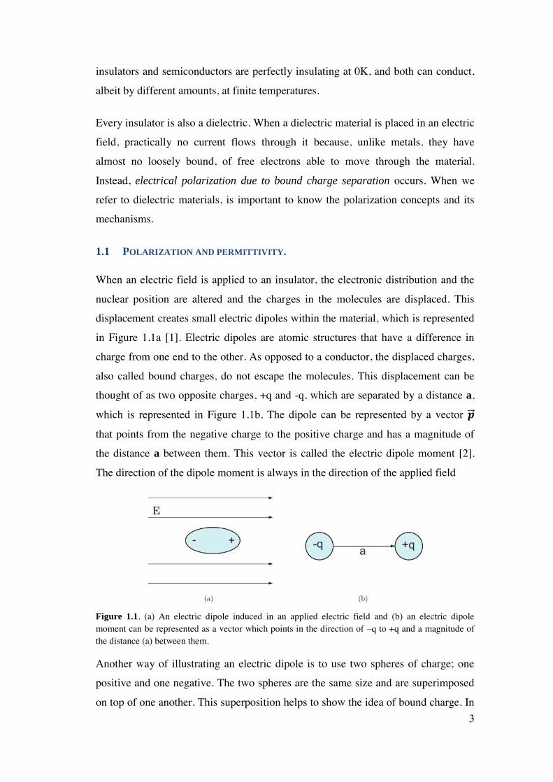
Figure 1.1. (a) An electric dipole induced in an applied electric field and (b) an electric dipole moment can be represented as a vector which points in the direction of –q to +q and a magnitude of the distance (a) between them.

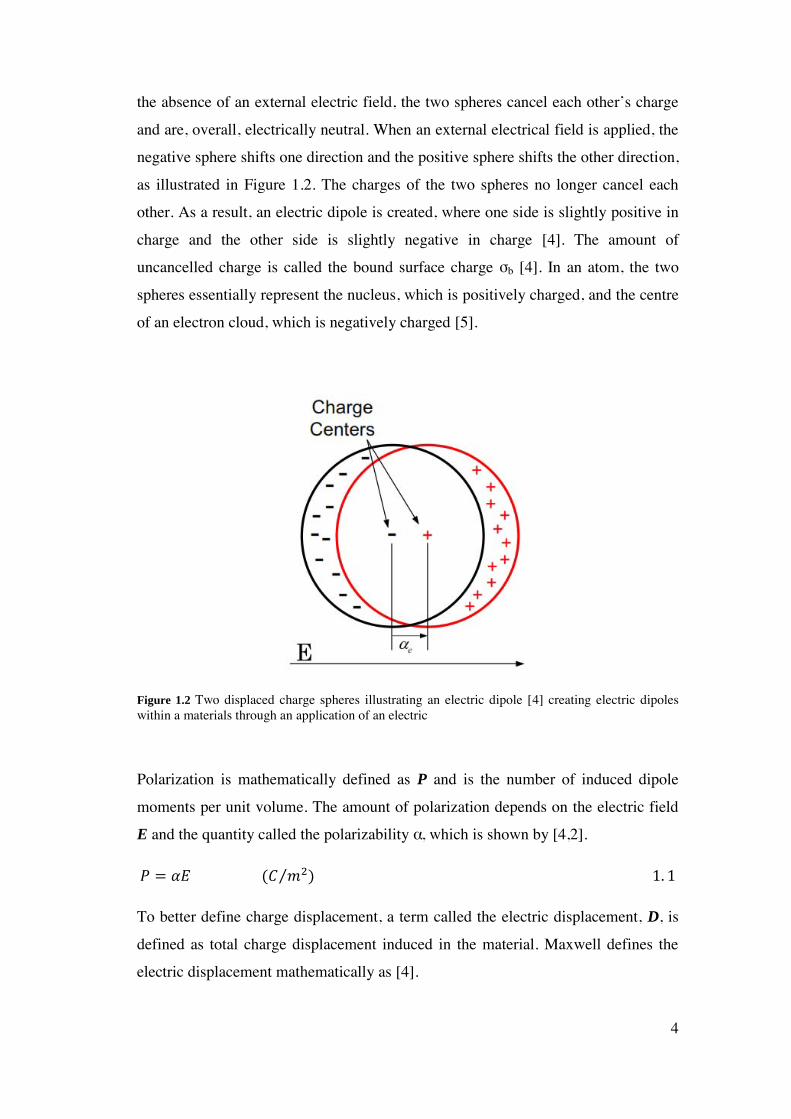
Another way of illustrating an electric dipole is to use two spheres of charge; one

positive and one negative. The two spheres are the same size and are superimposed

on top of one another. This superposition helps to show the idea of bound charge. In

4

the absence of an external electric field, the two spheres cancel each other’s charge

and are, overall, electrically neutral. When an external electrical field is applied, the

negative sphere shifts one direction and the positive sphere shifts the other direction,

as illustrated in Figure 1.2. The charges of the two spheres no longer cancel each

other. As a result, an electric dipole is created, where one side is slightly positive in

charge and the other side is slightly negative in charge [4]. The amount of

uncancelled charge is called the bound surface charge σb [4]. In an atom, the two

spheres essentially represent the nucleus, which is positively charged, and the centre

of an electron cloud, which is negatively charged [5].

Figure 1.2 Two displaced charge spheres illustrating an electric dipole [4] creating electric dipoles within a materials through an application of an electric

Polarization is mathematically defined as P and is the number of induced dipole

moments per unit volume. The amount of polarization depends on the electric field

E and the quantity called the polarizability α, which is shown by [4,2].

𝑃 = 𝛼𝐸 (𝐶 𝑚2⁄ ) 1. 1

To better define charge displacement, a term called the electric displacement, D, is

defined as total charge displacement induced in the material. Maxwell defines the

electric displacement mathematically as [4].

5

𝐷 = 휀0𝐸 + 𝑃 (𝐶 𝑚2⁄ ) 1. 2

Electric displacement consists of two parts, the displacement of charge which is a

result of the applied electric field and the displacement caused by polarization. The

induced dipole from the polarization induces its own electric field which further

contributes to the electric displacement.

The polarizability α of a dielectric can be divided into the electric susceptibility χe

and permittivity of free space ε0 [4]. The electric susceptibility is the dielectric’s

ability to be polarized, and the permittivity of free space is a universal polarizability

constant that is defined for all of free space. Incorporating the electronic

susceptibility, the number of induced dipoles per unit volume, Equation 1.1, then

turns into [4].

𝑃 = 𝜒𝑒휀0𝐸 (𝐶 𝑚2)⁄ 1.3

Substituting Equation 1.3 into Equation 1.2 yields [4].

𝐷 = 휀0𝐸 + 𝜒𝑒휀0𝐸

= 휀0(1 + 𝜒𝑒)𝐸 (𝐶 𝑚2⁄ ) 1.4

The permittivity of the material ε is defined as [4]

휀 = 휀0(1 + 𝜒𝑒) (𝐹 𝑚⁄ ) 1.5

Substituting Equation 1.5 into Equation 1.4 yields

𝐷 = 휀𝐸 (𝐶 𝑚2⁄ ) 1.6

As defined earlier, ε is the permittivity of the material and by dividing the

permittivity by the permittivity of free space yields the relative permittivity or the

dielectric constant, εr, and is defined as

휀𝑟 = 1 + 𝜒𝑒 =휀

휀0 1.7

The dielectric constant is one of the central themes in this study and is a key

characteristic in capacitor materials. The equations above illustrate the fact that the

dielectric constant defines how the dielectric material reacts to the introduction of an

6

electric field: the higher dielectric constant in a capacitor material causes a higher

electric energy density in the capacitor. Additionally, the dielectric constant also

affects the flexoelectric coefficient [6,7,8]: flexoelectricity is directly proportional to

permittivity. From a thermodynamical point of view, is flexoelectricity is one

mechanism for converting electric energy density into elastic energy density and

vice-versa, so anything that increases one should also increase the other. Ultimately,

both permittivty and flexoelectricity are measures of the polarizability of a material.

1.1.1 ELECTRONIC POLARIZATION.

Following the simple Bohr model of the atom, an applied electric field displaces the

electron orbit slightly (see Figure 1.3). This produces a dipole, equivalent to a

polarization. There are quantum mechanical treatments of this effect (using

perturbation or variational theory) which all give the result that the effect is both,

small and occurs very rapidly (on the timescale equivalent to the reciprocal of the

frequency of the X-ray or optical emission from excited electrons in those orbits).

Therefore we expect no delay in the occurrence of polarization after the application

of an electric field, and thus no dissipation phenomena, except at frequencies which

are resonant with the electron transition energies.

Figure 1.3. Electronic (atomic) polarization

After equilibrium is reached, the two forces acting on the electrons are the

coulombic attraction called the restoring force and the force due to the electric field

that keeps the electron cloud shifted. The average induced polarization per molecule

due to electronic polarization is [3] Thus:

𝑃𝑒 = 𝛼𝑒𝐸 (𝐶 𝑚2⁄ ) 1.8

7

As reflected earlier, the induced electronic dipole moment αe due to electronic

polarization is proportional to the electric field E. This equation is valid only under

equilibrium or static conditions.

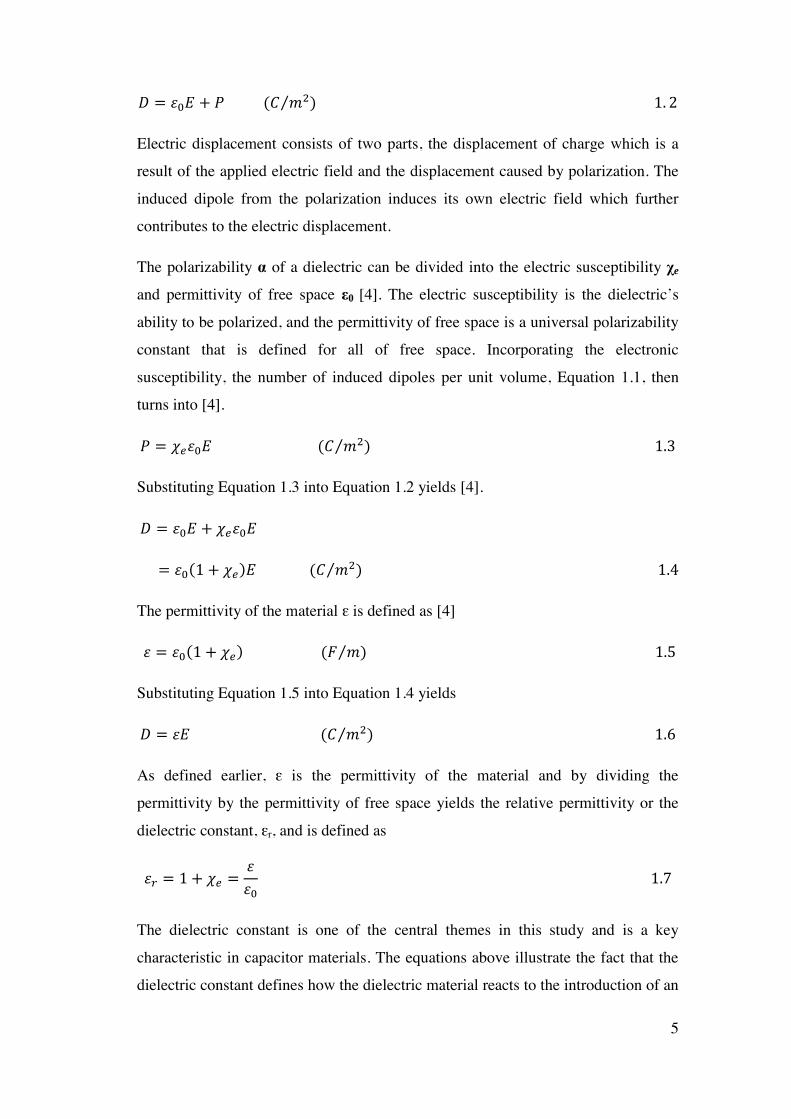
1.1.2 ELECTRONIC POLARIZATION IN COVALENT SOLIDS.

A covalent bond is a chemical bond that involves the sharing of electron pairs

between atoms. These electrons and their resulting wave functions are referred to as

delocalized. When an electric field is applied, two different types of electronic

polarizations can occur. The weaker one happens when the individual nuclei

experiences a shift within its own electron shell that is not shared with the lattice

bonds. The dominant one is the electronic polarization, based on the shifting of the

atom’s valence electrons and the lattice bonds surrounding the nuclei within the

material [9].

Figure 1.4 An illustration of electronic polarization in a Si covalent lattice (a) before the application

on an electric field and (b) after a field is applied [9].

1.1.3 IONIC POLARIZATION.

Ionic polarization occurs in crystal lattices of ionic molecules such as NaCl.

Although each individual molecule has a dipole moment, the net dipole moment of

the material is zero because the individual molecules are lined up head to head and

tail to tail, as shown in Figure 1.5. When an electric field is applied, cations and ions

are pushed in opposite directions, creating a net polarization in the material. The

average induced polarization per molecule due to ionic polarization is [9,10].

𝑃𝑖 = 𝛼𝑖𝐸 1.9

8

Where αi is the ionic polarization of the material, and E is the applied electric field.

Figure 1.5. Ionic polarization in NaCl [10]

1.1.4 ORIENTATIONAL POLARIZATION.

Polar molecules such as water have permanent dipole moments. In the liquid or gas

phase, these polar molecules can move around and are randomly orientated. When

an electric field is applied to a polar material, the dipoles experience a torque which

aligns them in the direction of the applied field. This process is called orientational

polarization [4, 9, 10].

Figure 1.6. A dielectric medium consisting of polar molecules (a) that are ramndomly oriented

before an electric field is applied and (b) after a field is applied

Some solids are made up of polar molecules which are normally randomly

orientated. There are materials such as certain plastics can be softened by heating

and exposed to an electric field in order to align the dipoles. The electric field is left

on as the material cools which solidifies the direction of the dipole moments. This

process is used to produce materials that have a permanent dipole moment. Electrets

and have many uses especially in high fidelity microphones [11].

9

The average induced polarization per molecule due to orientational polarization is

[9, 10]

𝑃0 = 𝛼0𝐸 1.10

Where α0 is the orientational polarization of the material, and E is the applied

electric field. As we shall see in chapters 3 and 4, the orientational polarization of

polar nanoregions that exist in relaxors and even standard ferroelectrics greatly

enhances their flexoelectric response.

1.1.5 INTERFACIAL POLARIZATION.

Even in the most pure of crystals and materials, there are defects and impurities that

generate charge carriers such as electrons, holes, and ions. These charge carriers can

move within the material and build up at different boundaries such as the dielectric-

electrode boundary or at grain boundaries within the material itself. This

accumulation also contributes to the dielectric constant of the material [3].

All of the above mechanisms of polarization are additive and define the total

polarization of the material. The average induced dipole moment per molecule is

[3].

𝑃𝑎𝑣 = 𝛼𝑒𝐸 + 𝛼𝑖𝐸 + 𝛼0𝐸 (𝐶 𝑚2⁄ ) 1.11

where αe is the electronic polarization, αi is the ionic polarization, α0 is the

orientational polarization, and E is the applied electric field. The interfacial

polarization is not added to the above equation because it occurs at interfaces and

does not correlate to an average polarization in the bulk material. This is again a

simplification because the electric field E in the above equation is the local field

experienced by the individual molecules and not the applied electric field [1, 3].

The take-home message from all the previous discussion is that polarization is a

complex magnitude that has several different contributions, all of which may be

potentially sensitive to strain gradients. Thus, the definition of flexoelectricity as a

dielectric (electronic+ionic) polarization generated by a strain gradient is

insufficient when attempting to correlate the actual experimental results (which

incorporate all possible contributions to the polarization) to their microscopic origin.

10

As will be seen, orientational and interfacial polarization can in some cases largely

dominate the total flexoelectric response of a material.

1.2 DIELECTRIC CONSTANT VS FREQUENCY.

The aforementioned polarization assumes a static electric field which does not vary

with time. The introduction of a time varying electric field adds a little more

complexity to the idea of polarization. The mechanics of polarization depends on the

movement of particles with mass. Particles have to be accelerated and shifted back

and forth as the electric field changes, which cannot occur instantaneously. Since

certain movements of particles involve the movement of different masses and

different distances, the different types of polarization will have different rates at

which polarization occurs. When a time varying electric field is applied, the

dielectric constant depends on the frequency of the field. As the frequency increases,

the different polarizations progressively show difficulties to follow the changes of

the electric field and start to relax. As a result, the slower processes cease to

contribute to the dielectric constant [1] as shown in Figure 1.7 [3]. At low

frequencies, all of the polarization types have time to reach their relaxed state. This

is important for our work because all our flexoelectric measurements have been

performed at low frequencies (of the order of 13Hz), and thus the measured

flexoelectric response is in principle sensitive to all polarization mechanisms.

1.3 DIELECTRIC LOSS.

An ideal dielectric material is a perfect insulator that only permits a displacement of

the charge by an electric field via polarization. In this sense, the impedance response

of a dielectric material is capacitive, and hence the generated displacement current

leads the voltage by 90°, or similarly is out of phase by a quarter-cycle. Real

materials always have dissipation and thus the phase angle between the current and

voltage is not exactly 90°; the current leads the voltage by 90- δ, where δ is defined

as the angle of lag. The angle of lag, δ, is the measure of the dielectric power loss.

𝑃𝑜𝑤𝑒𝑟 𝐿𝑜𝑠𝑠 = 𝜋𝑓𝑉02휀1𝑡𝑎𝑛𝛿 1.12

11

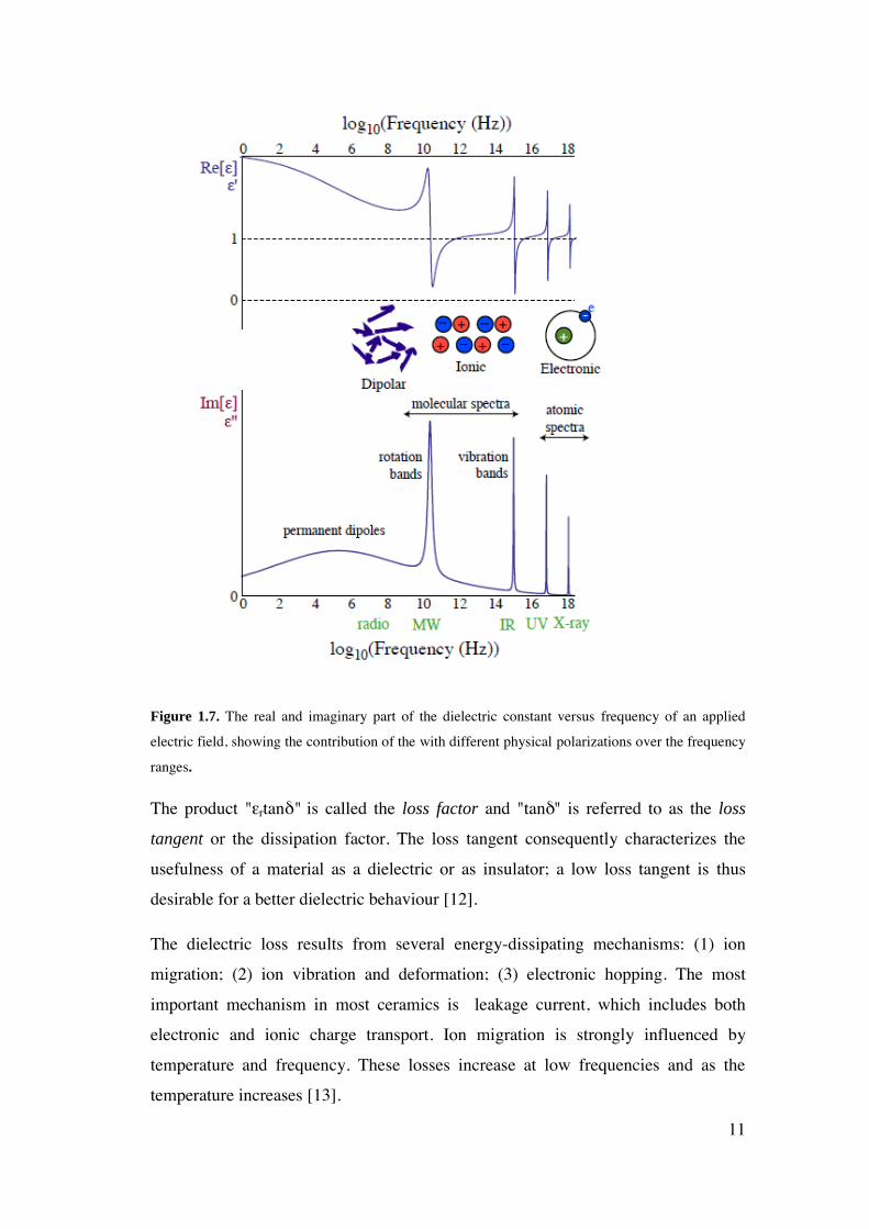
Figure 1.7. The real and imaginary part of the dielectric constant versus frequency of an applied

electric field, showing the contribution of the with different physical polarizations over the frequency

ranges.

The product "εrtanδ" is called the loss factor and "tanδ" is referred to as the loss

tangent or the dissipation factor. The loss tangent consequently characterizes the

usefulness of a material as a dielectric or as insulator; a low loss tangent is thus

desirable for a better dielectric behaviour [12].

The dielectric loss results from several energy-dissipating mechanisms: (1) ion

migration; (2) ion vibration and deformation; (3) electronic hopping. The most

important mechanism in most ceramics is leakage current, which includes both

electronic and ionic charge transport. Ion migration is strongly influenced by

temperature and frequency. These losses increase at low frequencies and as the

temperature increases [13].

12

Getting back to polarization, there are three main phenomena related to electric

dipoles: ferroelectricity, piezoelectricity and flexoelectricity. Ferroelectricity can

exist when there is a spontaneous alignment of electric dipoles by their mutual

interaction in the absence of an applied electric field, and is defined as the

reorientation (“switching”) of this spontaneous polarization upon application of a

finite electric field smaller than the breakdown strength of the material.

Piezoelectricity is defined as polarization induced by the application of external

force. The aforementioned properties are limited to materials with a non-

centrosymmetric crystal structure. In contrast, flexoelectricity is a universal

property, present in every material irrespective of their symmetry, and is defined as

the linear response of polarization to strain gradient. Polarization can, as discussed

earlier, be generated by dielectric separation of bound charge within atoms or unit

cells, or by a space charge separation of free carriers. To the best of our knowledge,

until now, when referring to flexoelectricity, only the response from bound charge

(electronic displacement within atoms or ionic displacement within unit cells) has

been taken into account. One of the main advances contained in this thesis and

developed in Chapter 5 is the observation that free carriers also respond to strain

gradients.

1.4 FERROELECTRICITY.

Ferroelectric materials (named “ferroelectrics”) have a spontaneous electric

polarization which can be switched by an external electric field. The spontaneous

polarization is produced by the arrangement of ions in the crystal structure, as in

conventional ferroelectrics, or on charge ordering as in electronic ferroelectrics

[14,15]. Only materials with a non-centrosymmetric point group which contains

alternate atom positions or molecular orientations to permit the reversal of the dipole

and the retention of polarization after voltage removal are ferroelectric.

Ferroelectricity is closely related to piezoelectricity and pyroelectricity; all

ferroelectric materials are also piezoelectric and pyroelectric, but not all

piezoelectrics are pyroelectric, and not all pyroelectrics are ferroelectric.[14]

The ferroelectric phase is typically reached by cooling from a high-symmetry, non-

polar phase through its Curie point (Tc), reducing the symmetry of the system and

permitting the polarization to align along any one of the crystallographically

13

equivalent directions. The ferroelectric phase can be represented by only minor

perturbations in the structure of the high-symmetry prototype phase, which is

paraelectric[14]. The paraelectric to ferroelectric phase transformation at Tc can be

either first order where the volume, strain, polarization and crystal structure of the

system change discontinuously at the transition point or second order where the

aforementioned parameters change continuously [17].

The Curie point is marked by a large dielectric anomaly, often in the form of a

diverging relative permittivity (εr). This can result in the appearance of a large peak

in permittivity at Tc. Many systems obey the Curie-Weiss law, which gives the

permittivity as a function of temperature above Tc as follows:

휀𝑟 =𝐶

𝑇−𝑇0 1.13

Where C is the Curie constant and T0 is the Curie temperature [16]. T0 is slightly

lower than Tc in the case of a first-order phase transition but is coincident with Tc in

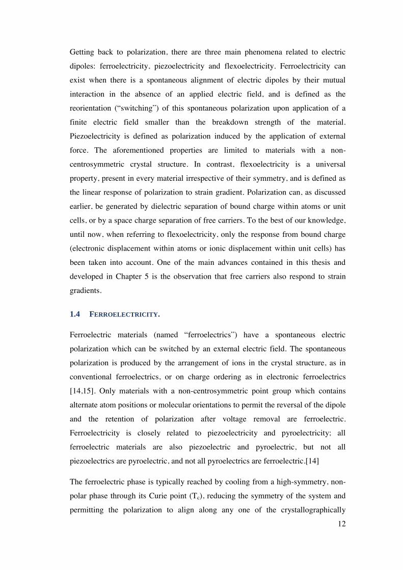
a second-order phase transition [17]. Below Tc, the spontaneous polarization in the

ferroelectric generally increases with decreasing temperature (i.e. 𝑑𝑃𝑆

𝑑𝑇< 0). This

behaviour is summarized in Figure 1.8.

Figure 1.8 Temperature dependence of the spontaneous polarization and permittivity in the ferroelectric material [16].

14

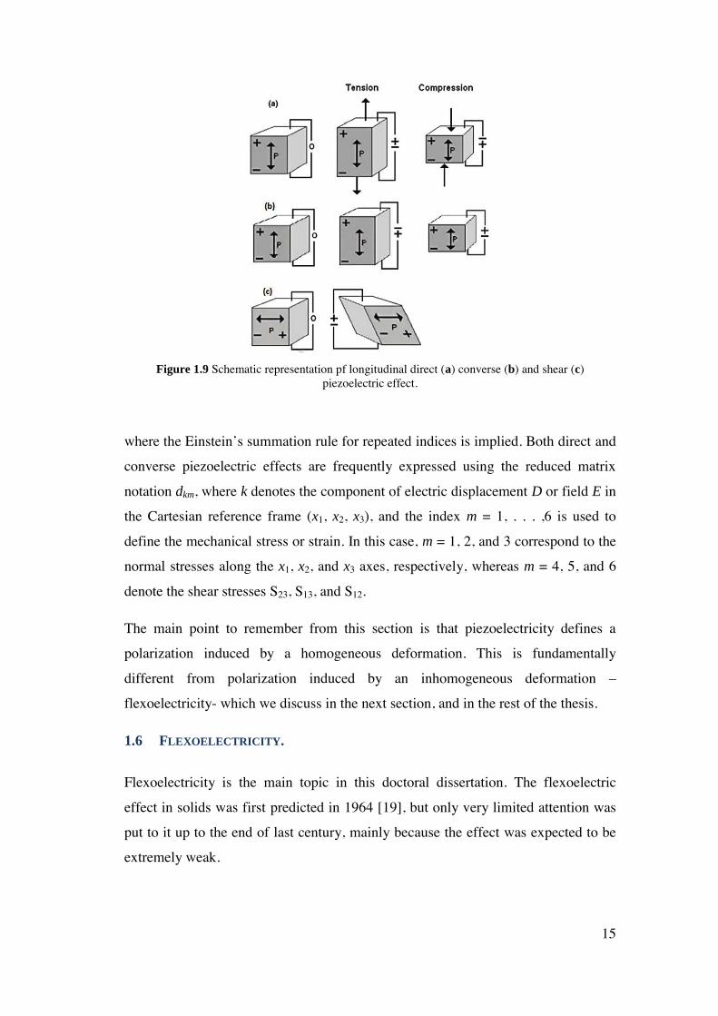
1.5 PIEZOELECTRICITY.

Piezoelectricity (following direct translation from Greek word piezein, “pressure

electricity”) was discovered by Jacques Curie and Pierre Curie as early as in 1880

(Curie and Curie 1880). This effect was distinguished from other similar phenomena

such as “contact electricity” (friction-generated static charge). Even at this stage, it

was clearly understood that symmetry plays a decisive role in the piezoelectric

effect, as it was observed only for certain crystal cuts and mostly in pyroelectric

materials in the direction normal to polar axis. However, the Curie brothers did not

predict a converse piezoelectric effect, i.e., deformation or stress under applied

electric field. This important property was then mathematically deduced from the

fundamental thermodynamic principles by Lippmann (1881). The existence of the

converse effect was immediately confirmed by Curie brothers. Since then, the term

piezoelectricity has thus been used for more than a century to describe the ability of

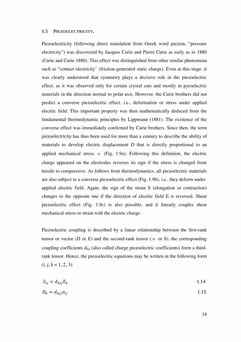
materials to develop electric displacement D that is directly proportional to an

applied mechanical stress σ (Fig. 1.9a). Following this definition, the electric

charge appeared on the electrodes reverses its sign if the stress is changed from

tensile to compressive. As follows from thermodynamics, all piezoelectric materials

are also subject to a converse piezoelectric effect (Fig. 1.9b), i.e., they deform under

applied electric field. Again, the sign of the strain S (elongation or contraction)

changes to the opposite one if the direction of electric field E is reversed. Shear

piezoelectric effect (Fig. 1.9c) is also possible, and it linearly couples shear

mechanical stress or strain with the electric charge.

Piezoelectric coupling is described by a linear relationship between the first-rank

tensor or vector (D or E) and the second-rank tensor (σ or S), the corresponding

coupling coefficients dkij (also called charge piezoelectric coefficients) form a third-

rank tensor. Hence, the piezoelectric equations may be written in the following form

(i, j, k = 1, 2, 3):

𝑆𝑖𝑗 = 𝑑𝑘𝑖𝑗𝐸𝑘 1.14

𝐷𝑘 = 𝑑𝑘𝑖𝑗𝜎𝑖𝑗 1.15

15

Figure 1.9 Schematic representation pf longitudinal direct (a) converse (b) and shear (c) piezoelectric effect.

where the Einstein’s summation rule for repeated indices is implied. Both direct and

converse piezoelectric effects are frequently expressed using the reduced matrix

notation dkm, where k denotes the component of electric displacement D or field E in

the Cartesian reference frame (x1, x2, x3), and the index m = 1, . . . ,6 is used to

define the mechanical stress or strain. In this case, m = 1, 2, and 3 correspond to the

normal stresses along the x1, x2, and x3 axes, respectively, whereas m = 4, 5, and 6

denote the shear stresses S23, S13, and S12.

The main point to remember from this section is that piezoelectricity defines a

polarization induced by a homogeneous deformation. This is fundamentally

different from polarization induced by an inhomogeneous deformation –

flexoelectricity- which we discuss in the next section, and in the rest of the thesis.

1.6 FLEXOELECTRICITY.

Flexoelectricity is the main topic in this doctoral dissertation. The flexoelectric

effect in solids was first predicted in 1964 [19], but only very limited attention was

put to it up to the end of last century, mainly because the effect was expected to be

extremely weak.

16

The flexoelectricity by definition is the response of electric polarization to a strain

gradient:

𝑃𝑖 = 𝜇𝑘𝑙𝑖𝑗

𝜕𝑢𝑘𝑙

𝜕𝑥𝑗 1.16

In contrast with the piezoelectricity, this effect is not limited to non-

centrosymmetric crystal structures, making it a more universal property.

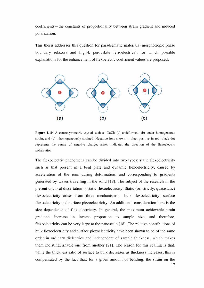
Homogeneous stress and strain cannot by themselves break centrosymmetry. If the

material is centrosymmetric(Figure 1.10a) and we apply a stress, the displacements

of ions are also symmetric and compensate each-other between them, so the result is

a null polarization (Figure 1.10b). In contrast, if the material is centrosymmetric and

we apply strain gradient, the displacement of ions is uncompensated and therefore a

net polarization can appear which is dictated by the direction of the strain gradient

(Figure 1.10c).

Estimation of flexoelectric coefficients was of the order of e/a, where e is the

electronic charge and a is the lattice parameter; it is a very small value of around

10-10 C/m for almost all insulators [19]. Bursian and Trunov [20], and then

Tagantsev [21], later predicted an enhancement of flexoelectric effect in materials

with high dielectric permittivity, a prediction backed up by first principle

calculations [6,7,8] and validated by multiple experimental work on relaxor

ferroelectrics and ferroelectric materials, such as Lead Magnesium Niobate ceramic

(PMN) [22], Barium Strontium Titanate ceramic (BST) [23], Lead Zirconate

Titanate ceramic (PZT)[24], Strontium Titanate single crystal (STO) [25] and

Barium Titanate ceramic (BTO) [26]. Measurements on BST and BTO also revealed

a remarkable magnitude of the flexoelectric coefficient in the order 10-5 C/m, which

is 103-105 times larger than the flexoelectric coefficient estimated by Kogan and is

too large even when the dielectric constant is factored in. With the exception of

SrTiO3[25], in fact, for most perovskites, the experimentally measured

flexoelectricity exceeds theoretical expectations by one to three orders of

magnitude[27, 30]. The origin of this enormous flexoelectric coefficient is not

known; the principal motivation for this thesis is precisely the remarkable lack of

fundamental knowledge about the intrinsic value of the effective flexoelectric

17

coefficients—the constants of proportionality between strain gradient and induced

polarization.

This thesis addresses this question for paradigmatic materials (morphotropic phase

boundary relaxors and high-k perovskite ferroelectrics), for which possible

explanations for the enhancement of flexoelectic coefficient values are proposed.

Figure 1.10. A centrosymmetric crystal such as NaCl: (a) undeformed, (b) under homogeneous

strain, and (c) inhomogeneously strained. Negative ions shown in blue, positive in red; black dot

represents the centre of negative charge; arrow indicates the direction of the flexoelectric

polarisation.

The flexoelectric phenomena can be divided into two types; static flexoelectricity

such as that present in a bent plate and dynamic flexoelectricity, caused by

acceleration of the ions during deformation, and corresponding to gradients

generated by waves travelling in the solid [18]. The subject of the research in the

present doctoral dissertation is static flexoelectricity. Static (or, strictly, quasistatic)

flexoelectricity arises from three mechanisms: bulk flexoelectricity, surface

flexoelectricity and surface piezoelectricity. An additional consideration here is the

size dependence of flexoelectricity. In general, the maximum achievable strain

gradients increase in inverse proportion to sample size, and therefore,

flexoelectricity can be very large at the nanoscale [18]. The relative contributions of

bulk flexoelectricity and surface piezoelectricity have been shown to be of the same

order in ordinary dielectrics and independent of sample thickness, which makes

them indistinguishable one from another [21]. The reason for this scaling is that,

while the thickness ratio of surface to bulk decreases as thickness increases, this is

compensated by the fact that, for a given amount of bending, the strain on the

18

surface (and thus its piezoelectricity) increases with sample thickness. Thus, the two

thickness dependences (surface-to-bulk ratio and of strain-induced polarization)

cancel each other, and the surface-piezoelectric contribution is therefore

independent of thickness. In contrast, surface flexoelectricity decreases in inverse

proportion to sample thickness, and can in principle be neglected from the analysis

of bulk samples; in this thesis, therefore, we have only dealt with bulk

flexoelectricity and surface piezoelectricity.

The impossibility of distinguishing between bulk flexoelectricity and surface

piezoelectricity by thickness-dependent studies has also meant that, so far, they have

been lumped together in effective coefficients that contain the contributions of both.

In this thesis, and for the first time, we provide direct experimental evidence for the

existence and magnitude of the surface piezoelectric effect. We have achieved this

by two different means: by changing the type of surface while leaving the bulk

contribution unchanged (chapter 4), and by screening the bulk contribution by

making the crystals conductive (chapter 5).

1.6.1 STATIC BULK FLEXOELECTRIC EFFECT.

This section describes the phenomenology of bulk flexoelectricity, which is the

principal topic of this doctoral dissertation. Static flexoelectricity has a different

treatment of dynamic flexoelectricity [31, 32].

For static case, the constitutive equation for electric polarization in a general

medium (including piezoelectricity) is [33]:

𝑃𝑖 = 𝜒𝑖𝑗𝐸𝑗 + 𝑒𝑖𝑗𝑘𝑢𝑗𝑘 + 𝜇𝑘𝑙𝑖𝑗

𝜕𝑢𝑘𝑙

𝜕𝑥𝑗 1.17

Where 𝐸𝑖, 𝑢𝑗𝑘 and 𝜕𝑢𝑗𝑘 𝜕𝑥𝑗⁄ are the macroscopic electric field, the strain tensor, and

its spatial gradient, respectively. In the equation 1.17, the first and the second terms

refer to dielectric and piezoelectric contributions with a second rank tensor 𝜒𝑖𝑗 and

third rank tensor 𝑒𝑖𝑗𝑘 respectively. The last term corresponds to the response of

polarization to a strain gradient- the flexoelectric effect- which is dictated by a

fourth rank tensor 𝜇𝑘𝑙𝑖𝑗. The flexoelectric tensor is allowed in any material, in

contrast with piezoelectricity which is limited to non-centrosymmetric materials.

19

Both flexoelectricity and piezoelectricity can describe properties of the materials in

the absence of a macroscopic electric field, so one can be define the following

tensor for piezoelectricity and flexoelecticity as:

𝑒𝑖𝑗𝑘 = (𝜕𝑃𝑖

𝜕𝑢𝑗𝑘)𝐸=0

1.18

𝜇𝑘𝑙𝑖𝑗 = (𝜕𝑃𝑖

(𝜕𝑢𝑘𝑙 𝜕𝑥𝑗⁄ ))

𝐸=0

1.19

Piezoelectricity and flexoelectricity are electromechanical phenomena that can be

described by thermodynamics. Therefore we can define the thermodynamic

potential density in terms of polarization, strain and their derivatives as [34].

Φ =𝜒𝑖𝑗

−1

2𝑃𝑖𝑃𝑗 +

𝑐𝑖𝑗𝑘𝑙

2𝑢𝑖𝑗𝑢𝑘𝑙 +

𝑔𝑖𝑗𝑘𝑙

2

𝜕𝑃𝑖

𝜕𝑥𝑗

𝜕𝑃𝑘

𝜕𝑥𝑙

−𝑓𝑖𝑗𝑘𝑙

2(𝑃𝑘

𝜕𝑢𝑖𝑗

𝜕𝑥𝑙− 𝑢𝑖𝑗

𝜕𝑃𝑘

𝜕𝑥𝑙) − 𝑃𝑖𝐸𝑖 − 𝑢𝑖𝑗𝜎𝑖𝑗 1.20

Where 𝑓𝑖𝑗𝑘𝑙 is called the flexocoupling tensor and has units of volts; this magnitude,

as we shall see, has a more universal value than the flexoelectric coefficient 𝜇. Static

bulk flexoelectricity was introduced by Indenbom [35], as a free energy in form of

equation 1.20.

Equations 1.20 contains again gradient terms. To find the equation of state it is

necessary to minimize the thermodynamic potential of the sample as a whole,

making a integration over volume of the sample as:∫Φ𝑑𝑉. For the latter procedure

one can use Euler equation 𝜕Φ 𝜕𝐴⁄ −𝑑

𝑑𝑥(𝜕Φ 𝜕(𝜕𝐴 𝜕𝑥⁄ )⁄ ) = 0, where A can be

replaced by P and x by u. In this way, the constitutive electromechanical equations

as proposed by Mindlin are[36]:

𝐸𝑖 = 𝜒𝑖𝑗−1𝑃𝑗 − 𝑓𝑘𝑙𝑖𝑗

𝜕𝑢𝑘𝑙

𝜕𝑥𝑗− 𝑔𝑖𝑗𝑘𝑙

𝜕2𝑃𝑖

𝜕𝑥𝑗𝜕𝑥𝑙 1.21

𝜎𝑖𝑗 = 𝑐𝑖𝑗𝑘𝑙𝑢𝑘𝑙 + 𝑓𝑖𝑗𝑘𝑙

𝜕𝑃𝑘

𝜕𝑥𝑙 1.22

20

Considering the polarization and strain gradient as homogeneous, the flexoelectric

effect described in equation 1.21 is the same as in equation 1.17 with:

𝜇𝑘𝑙𝑖𝑗 = 𝜒𝑖𝑠𝑓𝑘𝑙𝑠𝑗 1.23

Equation 1.23 couples the flexoelectric tensor to flexocoupling tensor through to

susceptibility of the material. The most important consequence of this equation is

that the flexoelectric coefficient is found to be proportional to the permittivity.

Therefore, materials with high dielectric constants such as ferroelectrics are good

candidates to study flexoelectricity. Additionally, Eq. 1.21 highlights that

flexoelectric coupling acts as an electric field (this can be seen by just moving the

second term of the right hand side to the left of the equality). This equivalence is

also important to understand that, just like all the components of the polarization of

a material (electronic, ionic, space-charge etc.) are sensitive to electric fields, they

can in principle be also responsive to flexoelectric fields, hence yielding a bigger

response than may have been anticipated from the ideal dielectric case considered

by Kogan.

On the other hand, equation 1.22, describes the contribution to mechanical stress

generated by a gradient of polarization, i.e. converse flexoelectricity.

From constitutive equation 1.21 and 1.22, and assuming the strain gradient is small

enough that the rhs term is vanished in equation 1.21, the equations of state can be

rewritten as.

𝑃𝑖 = 𝜒𝑖𝑗𝐸𝑗 + μ𝑘𝑙𝑖𝑗

𝜕𝑢𝑘𝑙

𝜕𝑥𝑗 1.24

𝜎𝑖𝑗 = 𝜇𝑖𝑗𝑘𝑙𝜕𝐸𝑘

𝜕𝑥𝑙+ 𝑐𝑖𝑗𝑘𝑙𝑢𝑘𝑙 1.25

These constitutive equations are convenient in the case of the extrinsic gradient,

such as mechanical bending of the sample as induced in the investigations of this

thesis, in contrast to the intrinsic strong gradient such as that at domain boundaries

or dislocations.

21

1.6.2 SURFACE PIEZOELETRIC EFFECT.

Surface contributions are always present in any phenomena on finite samples. In

general, this is small or even negligible because it is controlled by the ratio between

surface and volume; however in the present work, this effect is comparable to a bulk

effect and plays an important role in this doctoral dissertation. The relevant example

for this thesis is the surface piezoelectric effect, which is present even in

centrosymmetric materials; in these, the surface is breaks the symmetry and thus the

surface becomes a piezoelectric layer, with a thickness of λ.

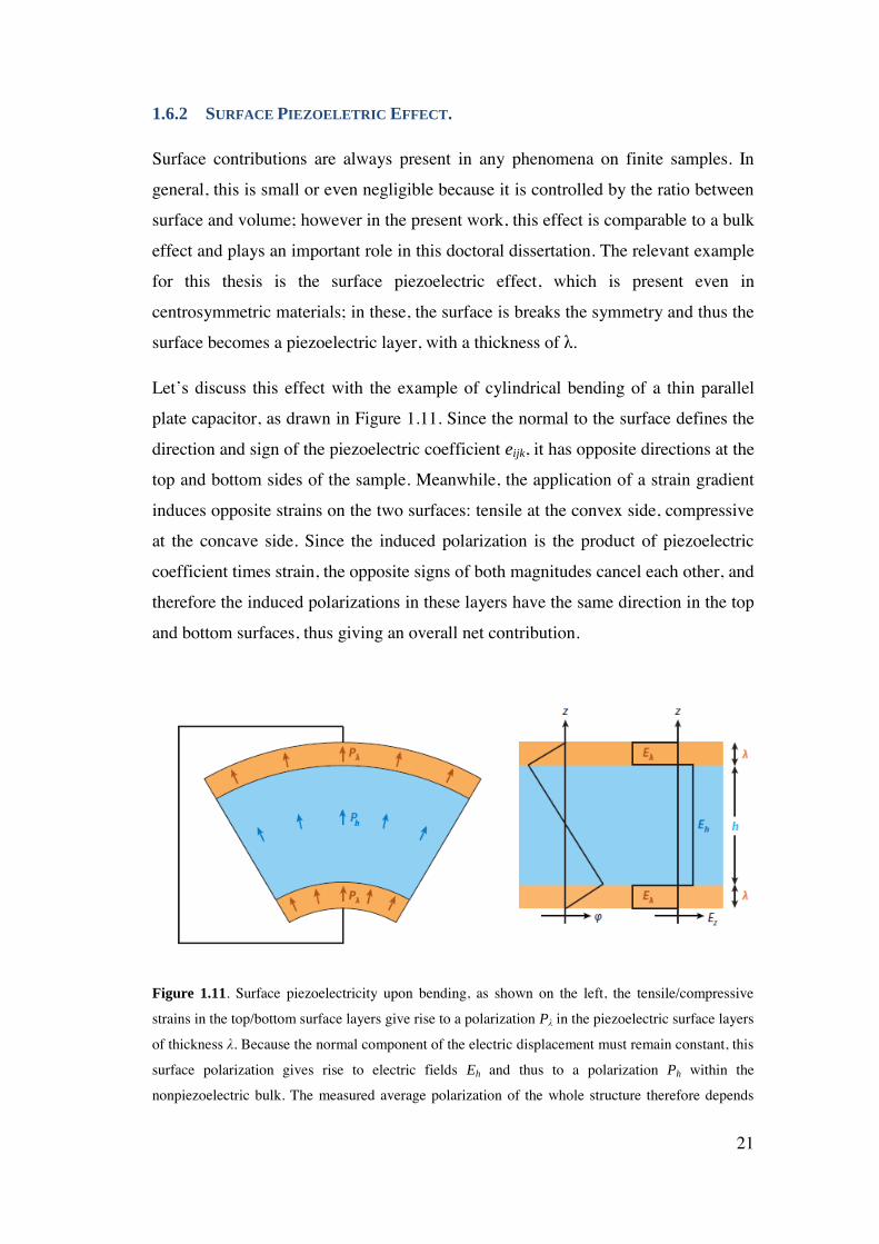
Let’s discuss this effect with the example of cylindrical bending of a thin parallel

plate capacitor, as drawn in Figure 1.11. Since the normal to the surface defines the

direction and sign of the piezoelectric coefficient eijk, it has opposite directions at the

top and bottom sides of the sample. Meanwhile, the application of a strain gradient

induces opposite strains on the two surfaces: tensile at the convex side, compressive

at the concave side. Since the induced polarization is the product of piezoelectric

coefficient times strain, the opposite signs of both magnitudes cancel each other, and

therefore the induced polarizations in these layers have the same direction in the top

and bottom surfaces, thus giving an overall net contribution.

Figure 1.11. Surface piezoelectricity upon bending, as shown on the left, the tensile/compressive

strains in the top/bottom surface layers give rise to a polarization Pλ in the piezoelectric surface layers

of thickness λ. Because the normal component of the electric displacement must remain constant, this

surface polarization gives rise to electric fields Eh and thus to a polarization Ph within the

nonpiezoelectric bulk. The measured average polarization of the whole structure therefore depends

22

not only on the dielectric properties of the piezoelectric surface layers but also on those of the bulk.

The potential ϕ and field E profiles along the sample thickness are shown on the right [18].

Additionally, the normal component of the electric displacement as described in the

equation 1.2, must be conserved across any dielectric interface, i.e., Dz = Pλ + ε0Eλ =

Ph + ε0Eh, where ε0 is the vacuum permittivity. Thus, internal fields appear in the

sample due to the presence of polarization Pλ within the surface layers. For a short-

circuited capacitor, the potential difference Δ = 2λEλ +hEh across the capacitor

must vanish; here h is the thickness of the nonpiezoelectric bulk (see Figure 1.11).

The electric displacement induced by the strain gradient can then be calculated as

[37]

𝐷 = 𝑒𝜆ℎ휀ℎ

2𝜆휀ℎ + ℎ휀𝜆

𝜕𝑢11

𝜕𝑥3 1.26

Where 휀𝜆 = 휀0 + 𝜒𝜆 is the dielectric constant of the surface layer and εh is that of the

bulk. For thin-enough surface layers (𝜆 ℎ⁄ ≪ 휀𝜆 휀ℎ⁄ ), and defining the effective

flexoelectric coefficient as the derivative of the displacement field with respect to

the strain gradient, Equation 1.26 yields an effective flexoelectric coefficient

associated with surface piezoelectricity:

𝜇1133𝑒𝑓𝑓

= 𝑒𝜆 ℎ

𝜆 1.27

The two ouststanding features of this equation are that (i) the polarization raising

from surface piezoelectriciticty is related with the bulk value of the dielectric

constant, and (ii) the effective flexoelectricity due to surface piezoelectricity is

independent of the thickness of the bulk (h). This means that, even for

macroscopically thick (bulk) samples, bending will provoke a surface response that

can in principle be as big as or even bigger than the actual bulk flexoelectricity of

the crystal. Moreover, for a quantitative evaluation of surface piezoelectric effect,

one can estimate the effective flexocoupling coefficient 𝑓𝑒𝑓𝑓 ≡ 𝜇𝑒𝑓𝑓 𝜒ℎ ≈ 𝑒𝜆 휀𝜆⁄⁄ .

For a conservative lower limit estimation, we consider the surface layer to be

atomically thin (λ = a few angstroms). Then, using e ∼ 1 C m−2 and 휀𝜆 휀0~10⁄ , we

find feff of the order of a few volts. This value is of the same order of magnitude as

23

the value of the components of the flexocoupling tensor fijkl∼1–10 V. Thus, surface

piezoelectricity can readily compete with bulk flexoelectricity.

The above features render surface piezoelectricity is qualitatively indistinguishable

from bulk flexoelectricity. The only way to separate the two effects (bulk flexo and

surface piezo) are therefore to either (i) change the nature of the surface, so that its

surface-piezoelectric coefficient e is changed while preserving the same value of the

bulk flexoelectric coefficient [38] or (ii) screen the bulk flexoelectricity by making

the bulk conducting while keeping the interface insulating. The first route is

described in chapter (4) and the second in chapter (5) of this thesis.

1.7 MATERIALS.

Below the Curie temperature TC, ferroelectric materials undergo a phase transition

from paraelectric to ferroelectric [39, 40]. In proper ferroelectrics (i.e., those where

polarization is the primary order parameter), the dielectric constant shows a peak at

the Curie temperature. Meanwhile, relaxors show a more diffuse phase transition

with a high but broad dielectric peak, persistence of polar nanoregions even in the

nominally paraelectric phase, and lack of spontaneous (i.e. not field-induced) long-

range order. Solid solutions between ferroelectrics and relaxors can yield

morphotropic phase boundary materials that are at the frontier between ferroelectric

and relaxor behaviours.

The transformation plasticity associated with such morphotropic phase boundaries

renders these frontier materials as the best electromechanical ceramics known to

man [41].

The high dielectric constant of relaxor-ferroelectric and ferroelectric materials also

makes them good candidates to obtain high flexoelectric performance. Therefore,

for this thesis we investigated archetypical examples of each type: (1-

x)Pb(Mg1/3Nb2/3)O3-xPbTiO3, with x = 0.28 and 0.34 (hereafter, labelled PMN-

28%PT and PMN-34%PT) as morphotropic phase boundary Relaxor Material

(Chapter 3) and BaTiO3 (Chapter 4) as Ferroelectric Material.

In Chapter 5, we have studied the role of conductivity. We have used oxygen

reduction and annealing in determining the flexoelectric coefficient values in (001)-

24

oriented BTO single crystal. When reduced, more electrons per unit volume are

available to carry a current under applied field. In these conditions, the current in the

reduced material can be expressed as the sum of two contributions: the

displacement current, resulting from changes in dielectric polarization, and the free

charge current resulting from the movement of free carriers (oxygen vacancies) in

response to the applied strain gradient. In the conductive conditions we found a

colossal flexoelectric values and therefore conclude that the flexoelectric property is

not limited to dielectric materials, but should be extended to semiconductor

materials. Based on this observation, we have also initiated the study of

flexoelectricity in an archetypical semiconductor such as silicon, which is discussed

in chapter 6.

1.8 REFERENCES.

1. L. V. Azaroff and J. J. Brophy, Electronic Processes in Materials. McGraw Hill,

1963.

2. P. W. Atkins, Physical Chemistry, 4th Ed. W.H. Freeman and Company, 1990.

3. S. O. Kasap, Principles of electrical engineering materials and devices. McGraw

Hill, 2000.

4. D. J. Griffiths, Introduction to Electrodynamics, 2nd Ed. Prentice Hall, 1989.

5. F. T. Ulaby, Fundamentals of Applied Electromagnetics. Pearson Prentice Hall,

2004.

6. I. Ponomareva, A. K. Tagantsev, and L. Bellaiche, Phys. Rev. B. 85, 104101

(2012).

7. J. Hong and D. Vanderbilt, Phys. Rev. B. 88, 174107 (2013).

8. M. Stengel, Phys. Rev. B. 88, 174106 (2013).

9. S. O. Kasap, Principles of electrical engineering materials and devices. McGraw

Hill, 2000.

10. W. D. J. Callister, Materials Science and Engineering, 3rd Ed. John Wiley and

Sons, Inc., 1994.

25

11. D. K. Cheng, Field and Wave Electromagnetics, 2nd Ed. Addison-Wesley

Publishing Company, 1992

12. R. M. Rose, L. A. Shepard, and J. Wulff, “The structure and properties of

materials”, Wiley Eastern private limited, (1971).

13. D. W. Richerson, "Modern ceramic engineering: Properties, processing, and use

in design", Second Edition, Marcel Dekker, inc., (1992).

14. M. E. Lines and A.M. Glass, “Principles and Spplications of Ferrroelectric and

related Materials”Oxford (1977)

15. K. M. Rabe, M. Dawber, C. Lichtensteiger, C. H. Ahn and J-M. Triscone,

“Modern Physics od Ferroelecttrics: Essential Background”, Springer, 2007

16. K. Uchino, “Piezoelectric actuators and ultrasonic motors”. Boston: Kluwer Academic Piblisers. (1997)

17. T. Mitsui, I. Tatsuzaki, and E. Nakamura, “An introduction to the physics of ferroelectrics.” New York: Gordon and Breach Science Publishers (1976)

18. P. Zubko, G. Catalan and A. K. Taganstsev, Annu. Rev. Mater. Res. 43 (2013).

19. S. M. Kogan Sov. Phys.Solid. State. 5, 2069 (1964).

20. E. V. Bursian, N.N. Trunov, Sov. Phys. Sol. State. 16, 760 (1974).

21. A. K. Tagantsev, Phys. Rev. B. 34, 5883 (1986).

22. W. Ma and L. E. Cross, Appl. Phys. Lett. 78, 2920 (2001).



25. P. Zubko, G. Catalan, A. Buckley, P. R. L Welche, and J. F Scott., Phys. Rev.

Lett. 99, 167601 (2007).


27. R. Marangati and P. Sharma, Phys. Rev. B. 80, 054109 (2009).

26

28. J. Hong, G.Catalan, J.F.Scott and E. Artacho, J. Phys.: Condens. Matter. 22,

112201 (2010).


30. L. Shu, X. Wei, L. Jin, Y. Li, H. Wang, and X. Yao, Appl. Phys. Lett. 102,

152904 (2013).

31. A. K. Tagantsev, Phase. Transit. 35, 119 (1991)

32. A. K. Tagantsev, Phys. Rev. B. 34, 5883 (1986)

33. S. M. Kogan, Phys. Solid. State. 5, 2069 (1964)

34. P. V. Yudin and A. K Tagantsev, Nanotechnology, 24, 432001 (2013)

35. V.L. Indenbom, E. B. Loginov and M. A. Osipov, Kristalografija, 26, 1157

(1981)

36. R. D. Mindlin. Int. J. Solids Struct. 4, 637 (1968)

37. A.K. Tagantsev, A.S. Yurko., J. Appl. Phys. 112, 044103 (2012)

38. M. Stengel, Phys. Rev. B. 90, 201112(R) (2014).

39. A. F. Devonshire, Philos. Mag. 40, 1040, (1949).

40. A. Von. Hippel, Rev. Mod. Phys. 22, 221 (1950).

41. S-E Park and T. R. Shrout. J. Appl. Phys. 82, 1804 (1997)

27

2 EXPERIMENTAL PROCEDURES

28

As a starting point, it is important to emphasize that there is not any commercial

standard equipment in the market for flexoelectric measurements, such as there is

for example to perform dielectric measurements (LCR-Meter), polarization loops

(RT66B), etc. Therefore, the first step of this thesis work was to implement our own

system to measure flexoelectricity. The designed set-up was based on a Dynamical

Mechanical Analyzer (DMA) on which we implemented the simultaneous detection

of bending induced current with external instrumentation such as a home-made

signal amplifier and a lock-in amplifier. Every aforementioned instrument was

controlled with programs made in LabView software. LabView allows us to obtain a

versatile and user-friendly interface for integrating electric, mechanical and

electromechanical measurements as a function of various parameters, including

temperature. In the following, each step of this hardware and software development

is exposed.

2.1 MECHANICAL MEASUREMENTS BY DYNAMIC MECHANICAL ANALYSIS

A dynamic mechanical analyser (DMA) is an instrument that allows us measure the

mechanical response (deformation and mechanical loss) of a material as it is

subjected to a periodic force. The material response is expressed in terms of a

dynamic young’s modulus and a dynamic loss modulus (a mechanical damping

term). Typically, the values of dynamic moduli depend upon the type of material,

temperature, and frequency of the measurement.

For an applied sinusoidal stress, a material will respond with a sinusoidal strain for

low amplitudes of stress. The sinusoidal variation in time is usually described as a

rate specified by the frequency (f = Hz; = rad/sec). The strain of a material is out

of phase with the stress applied, by the phase angle, δ. This phase lag is due to the

excess time necessary for molecular motions and relaxations to occur. The dynamic

stress thus precedes the strain by δ, and the dynamic stress, σ, and strain, ε, are

given as:

𝜎 = 𝜎0 sin(𝜔𝑡 + 𝛿) 2.1

휀 = 휀0 sin(𝜔𝑡) 2.2

29

where is the angular frequency. Stress can be divided into an “in-phase”

component (σ0cos δ) and an “out-of-phase” component (σ0sin δ) and rewritten as.

𝜎 = 𝜎0 sin(𝜔𝑡) cos 𝛿 +𝜎0 cos(𝜔𝑡) sin 𝛿 2.3

Dividing stress by strain yields to the Young’s modulus E of the sample and using

the symbols E’ and E’’ for the in phase (real) and out-of-phase (imaginary)

components yields to:

𝜎 = 휀0 E′sin(𝜔𝑡) + 휀0 E′′cos(𝜔𝑡) 2.4

𝐸′ =𝜎0

휀0cos 𝛿 𝐸′′ =

𝜎0

휀0sin 𝛿 2.5

In the frequency domain, this relationship can be expressed as:

휀 = 휀0exp (𝑖𝜔𝑡) 𝜎 = 𝜎0exp (𝜔𝑡 + 𝛿)𝑖 2.6

𝐸∗ =𝜎

휀=

𝜎0

휀0𝑒𝑖𝛿 =

𝜎0

휀0

(cos 𝛿 + 𝑖 sin 𝛿) = 𝐸′ + 𝑖𝐸′′ 2.7

where E’ is the Young’s modulus and E’’ is the loss modulus. The phase angle δ is

given by

tan 𝛿 =𝐸′′

𝐸′ 2.8

Equation 2.7 shows that the complex modulus obtained from a dynamic mechanical

test consist of “real” and “imaginary” parts. The real (storage) part describes the

ability of the material to store potential energy and release it upon deformation, i.e.,

it describes the elastic part of the mechanical response. The imaginary (loss) portion

is associated with energy dissipation in the form of heat upon deformation.

The storage modulus is often times associated with “stiffness” of a material and is

related to the Young’s modulus, E. The dynamic loss modulus is often associated

with “internal friction” and is sensitive to different kinds of molecular motions,

relaxation processes such as dislocations or twin formation, transitions, morphology

and other structural heterogeneities. Thus, the dynamic properties provide

information at the molecular level to understand the material mechanical behaviour.

30

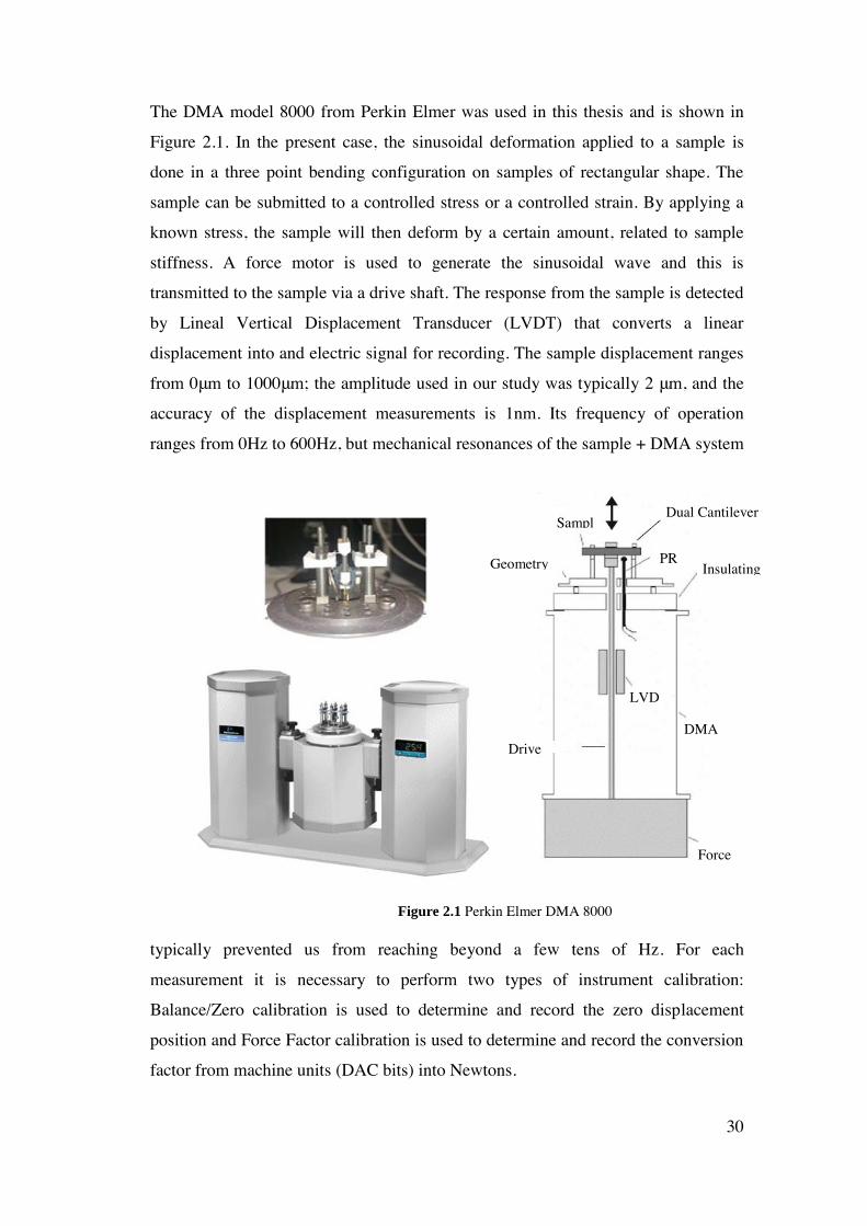
The DMA model 8000 from Perkin Elmer was used in this thesis and is shown in

Figure 2.1. In the present case, the sinusoidal deformation applied to a sample is

done in a three point bending configuration on samples of rectangular shape. The

sample can be submitted to a controlled stress or a controlled strain. By applying a

known stress, the sample will then deform by a certain amount, related to sample

stiffness. A force motor is used to generate the sinusoidal wave and this is

transmitted to the sample via a drive shaft. The response from the sample is detected

by Lineal Vertical Displacement Transducer (LVDT) that converts a linear

displacement into and electric signal for recording. The sample displacement ranges

from 0μm to 1000μm; the amplitude used in our study was typically 2 μm, and the

accuracy of the displacement measurements is 1nm. Its frequency of operation

ranges from 0Hz to 600Hz, but mechanical resonances of the sample + DMA system

typically prevented us from reaching beyond a few tens of Hz. For each

measurement it is necessary to perform two types of instrument calibration:

Balance/Zero calibration is used to determine and record the zero displacement

position and Force Factor calibration is used to determine and record the conversion

factor from machine units (DAC bits) into Newtons.

Dual Cantilever jig Sampl

e PRT Insulating

disk Geometry disk

LVDT

DMA chassis Drive

shaft

Force motor

Figure 2.1 Perkin Elmer DMA 8000

31

Finally, the DMA is embedded in a wide range furnace machinery capable of

operating at temperatures between -150ºC and 600ºC. This includes a standard

furnace configuration for heating and a cooling circuit for liquid nitrogen assisted

cooling and controlled temperature ramping. Liquid nitrogen is driven through

accessory circuit from a liquid nitrogen storage dewar of 50L placed by the set up.

The temperature change rate of DMA can be varied by setting it from 1ºC/min to

10ºC/min. It must be mentioned, however, that although this the temperature range

in which mechanical measurements can be made, electromechanical measurements

such as flexoelectricity require making electrical connections to the sample, and not

all wires can resist exposure to high temperatures. This wiring is not part of the as-

purchased DMA and we had to implement it ourselves; details are described in the

next section.

2.2 FLEXOELECTRIC MEASUREMENTS.

2.2.1 STRAIN GRADIENTS BY DYNAMIC MECHANICAL ANALYSIS

The main experimental task of this thesis was to measure the flexoelectric response

of single crystals. In order to generate flexoelectric polarization, a strain gradient

was applied by bending the samples.

The strain gradient along the direction of thickness was induced by a three-point

bending motion, as illustrated in Figure 2.2. Samples are supported (but not

clamped) on both ends by fixed sharp bars, and the drive shaft applies the

deformation by pressing in the middle of the sample. The maximum dynamic

displacement delivered to the middle of the samples was around 2 μm.

The strain of each measurement was calculated from the usual equation for a bent

beam:

𝜖11 =24𝑥3

𝐿3(𝐿

2− 𝑥1) 𝑧0 2.8

where z0 is the displacement applied to the sample from the DMA, L is the length

between the shafts, and x1 and x3 are spatial coordinates. Therefore, the strain

gradient in the normal to the surface is:

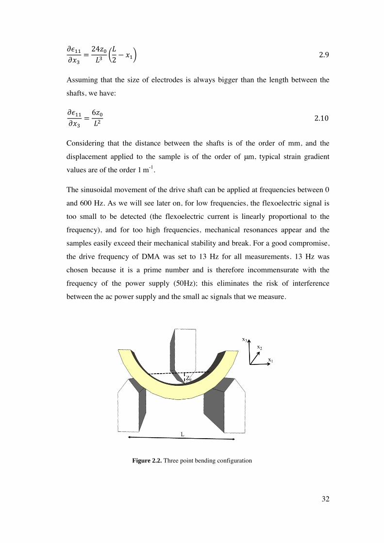
32

𝜕𝜖11

𝜕𝑥3=

24𝑧0

𝐿3(𝐿

2− 𝑥1) 2.9

Assuming that the size of electrodes is always bigger than the length between the

shafts, we have:

𝜕𝜖11

𝜕𝑥3=

6𝑧0

𝐿2 2.10

Considering that the distance between the shafts is of the order of mm, and the

displacement applied to the sample is of the order of μm, typical strain gradient

values are of the order 1 m-1.

The sinusoidal movement of the drive shaft can be applied at frequencies between 0

and 600 Hz. As we will see later on, for low frequencies, the flexoelectric signal is

too small to be detected (the flexoelectric current is linearly proportional to the

frequency), and for too high frequencies, mechanical resonances appear and the

samples easily exceed their mechanical stability and break. For a good compromise,

the drive frequency of DMA was set to 13 Hz for all measurements. 13 Hz was

chosen because it is a prime number and is therefore incommensurate with the

frequency of the power supply (50Hz); this eliminates the risk of interference

between the ac power supply and the small ac signals that we measure.

Figure 2.2. Three point bending configuration

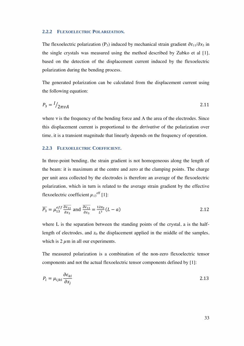
33

2.2.2 FLEXOELECTRIC POLARIZATION.

The flexoelectric polarization (P3) induced by mechanical strain gradient 𝜕ε11/𝜕x3 in

the single crystals was measured using the method described by Zubko et al [1],

based on the detection of the displacement current induced by the flexoelectric

polarization during the bending process.

The generated polarization can be calculated from the displacement current using

the following equation:

𝑃3 = 𝐼2𝜋𝑣𝐴⁄ 2.11

where ν is the frequency of the bending force and A the area of the electrodes. Since

this displacement current is proportional to the derivative of the polarization over

time, it is a transient magnitude that linearly depends on the frequency of operation.

2.2.3 FLEXOELECTRIC COEFFICIENT.

In three-point bending, the strain gradient is not homogeneous along the length of

the beam: it is maximum at the centre and zero at the clamping points. The charge

per unit area collected by the electrodes is therefore an average of the flexoelectric

polarization, which in turn is related to the average strain gradient by the effective

flexoelectric coefficient µ13eff [1]:

𝑃3 = 𝜇13

𝑒𝑓𝑓 𝜕𝜖11

𝜕𝑥3 and

𝜕𝜖11

𝜕𝑥3=

12𝑧0

𝐿3(𝐿 − 𝑎) 2.12

where L is the separation between the standing points of the crystal, a is the half-

length of electrodes, and z0 the displacement applied in the middle of the samples,

which is 2 µm in all our experiments.

The measured polarization is a combination of the non-zero flexoelectric tensor

components and not the actual flexoelectric tensor components defined by [1]:

𝑃𝑖 = 𝜇𝑖𝑗𝑘𝑙

𝜕𝜖𝑘𝑙

𝜕𝑥𝑗 2.13

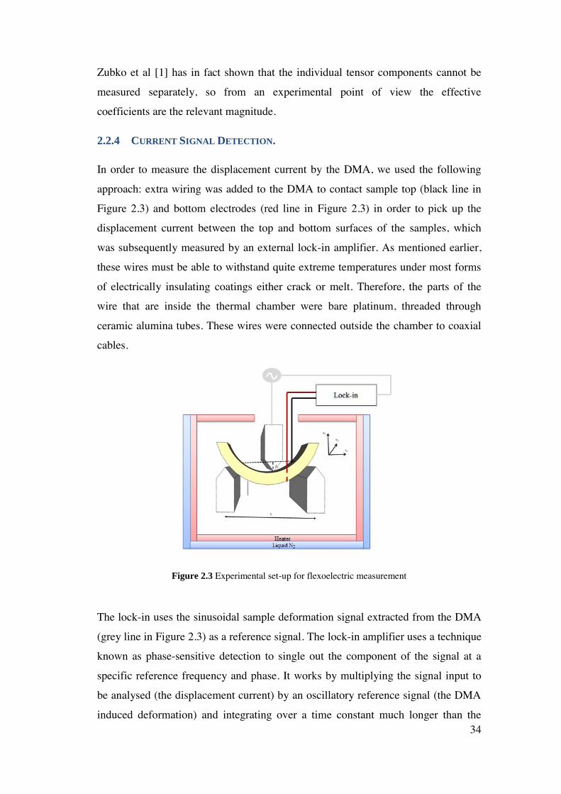
34

Zubko et al [1] has in fact shown that the individual tensor components cannot be

measured separately, so from an experimental point of view the effective

coefficients are the relevant magnitude.

2.2.4 CURRENT SIGNAL DETECTION.

In order to measure the displacement current by the DMA, we used the following

approach: extra wiring was added to the DMA to contact sample top (black line in

Figure 2.3) and bottom electrodes (red line in Figure 2.3) in order to pick up the

displacement current between the top and bottom surfaces of the samples, which

was subsequently measured by an external lock-in amplifier. As mentioned earlier,

these wires must be able to withstand quite extreme temperatures under most forms

of electrically insulating coatings either crack or melt. Therefore, the parts of the

wire that are inside the thermal chamber were bare platinum, threaded through

ceramic alumina tubes. These wires were connected outside the chamber to coaxial

cables.

Figure 2.3 Experimental set-up for flexoelectric measurement

The lock-in uses the sinusoidal sample deformation signal extracted from the DMA

(grey line in Figure 2.3) as a reference signal. The lock-in amplifier uses a technique

known as phase-sensitive detection to single out the component of the signal at a

specific reference frequency and phase. It works by multiplying the signal input to

be analysed (the displacement current) by an oscillatory reference signal (the DMA

induced deformation) and integrating over a time constant much longer than the

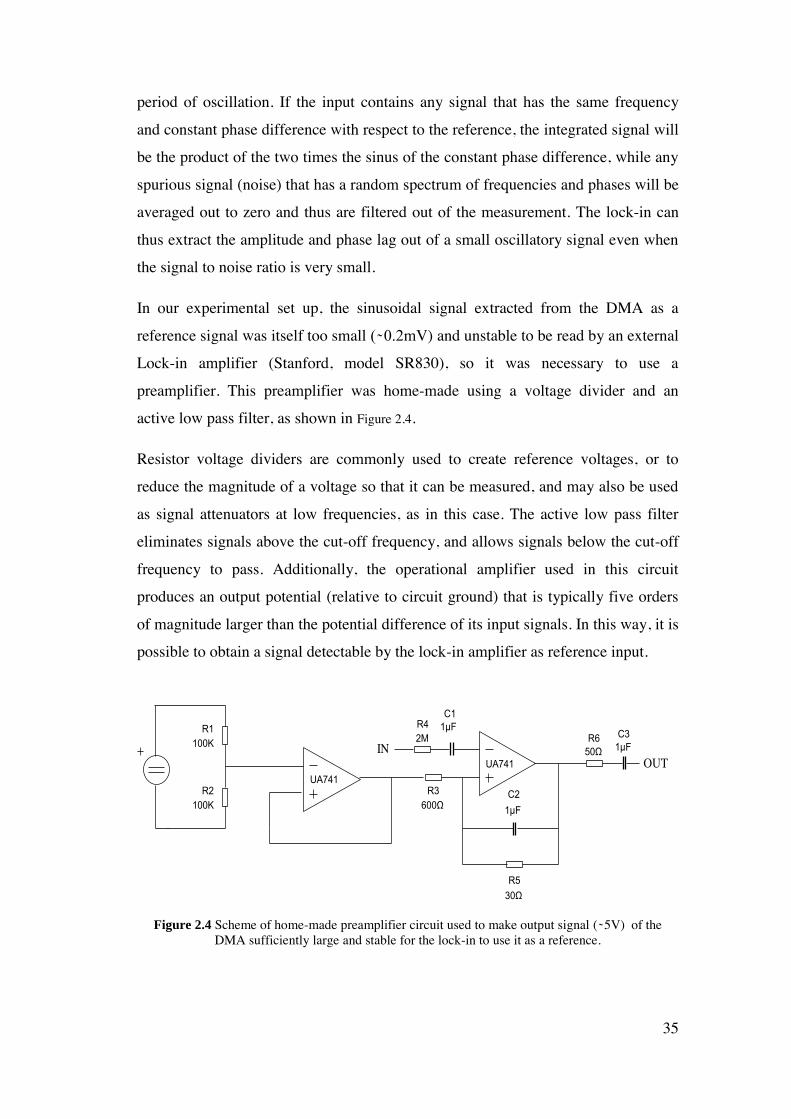
35

period of oscillation. If the input contains any signal that has the same frequency

and constant phase difference with respect to the reference, the integrated signal will

be the product of the two times the sinus of the constant phase difference, while any

spurious signal (noise) that has a random spectrum of frequencies and phases will be

averaged out to zero and thus are filtered out of the measurement. The lock-in can

thus extract the amplitude and phase lag out of a small oscillatory signal even when

the signal to noise ratio is very small.

In our experimental set up, the sinusoidal signal extracted from the DMA as a

reference signal was itself too small ( 0.2mV) and unstable to be read by an external

Lock-in amplifier (Stanford, model SR830), so it was necessary to use a

preamplifier. This preamplifier was home-made using a voltage divider and an

active low pass filter, as shown in Figure 2.4.

Resistor voltage dividers are commonly used to create reference voltages, or to

reduce the magnitude of a voltage so that it can be measured, and may also be used

as signal attenuators at low frequencies, as in this case. The active low pass filter

eliminates signals above the cut-off frequency, and allows signals below the cut-off

frequency to pass. Additionally, the operational amplifier used in this circuit

produces an output potential (relative to circuit ground) that is typically five orders

of magnitude larger than the potential difference of its input signals. In this way, it is

possible to obtain a signal detectable by the lock-in amplifier as reference input.

Figure 2.4 Scheme of home-made preamplifier circuit used to make output signal ( 5V) of the DMA sufficiently large and stable for the lock-in to use it as a reference.

UA741UA741

C31µF

C21µF

C11µFR1

100K

R2100K

R3600Ω

R530Ω

R42M R6

50ΩINOUT

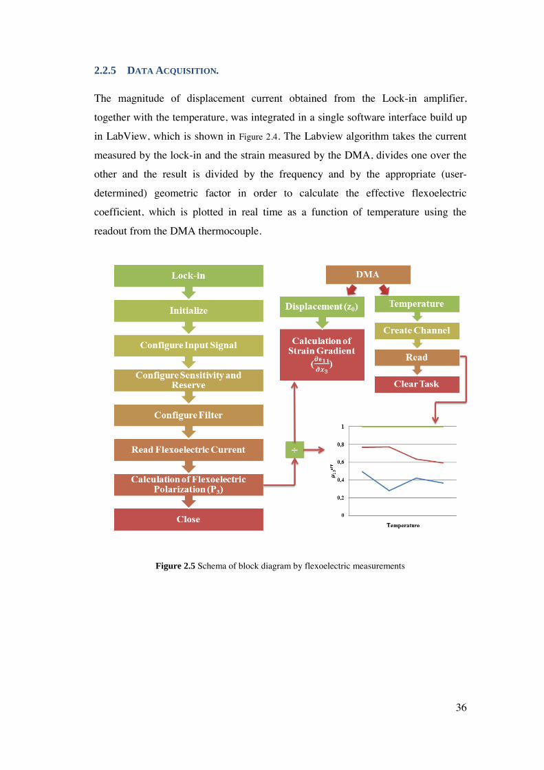
36

2.2.5 DATA ACQUISITION.

The magnitude of displacement current obtained from the Lock-in amplifier,

together with the temperature, was integrated in a single software interface build up

in LabView, which is shown in Figure 2.4. The Labview algorithm takes the current

measured by the lock-in and the strain measured by the DMA, divides one over the

other and the result is divided by the frequency and by the appropriate (user-

determined) geometric factor in order to calculate the effective flexoelectric

coefficient, which is plotted in real time as a function of temperature using the

readout from the DMA thermocouple.

Figure 2.5 Schema of block diagram by flexoelectric measurements

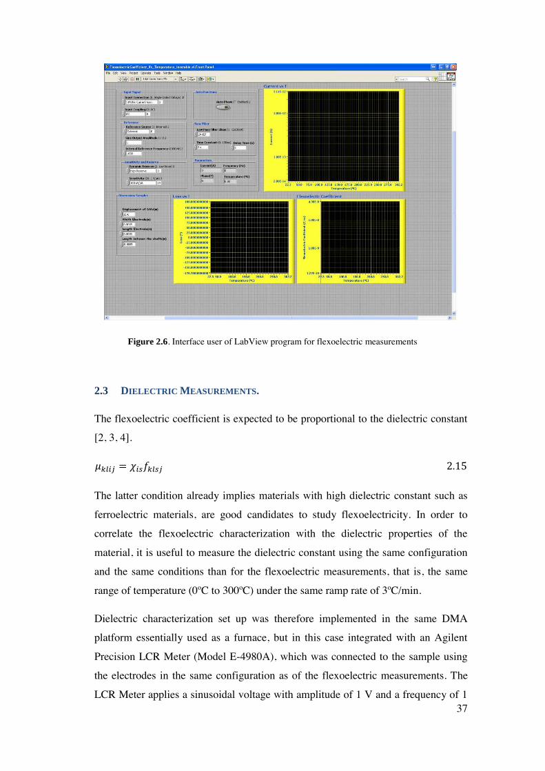
37

Figure 2.6. Interface user of LabView program for flexoelectric measurements

2.3 DIELECTRIC MEASUREMENTS.

The flexoelectric coefficient is expected to be proportional to the dielectric constant

[2, 3, 4].

𝜇𝑘𝑙𝑖𝑗 = 𝜒𝑖𝑠𝑓𝑘𝑙𝑠𝑗 2.15

The latter condition already implies materials with high dielectric constant such as

ferroelectric materials, are good candidates to study flexoelectricity. In order to

correlate the flexoelectric characterization with the dielectric properties of the

material, it is useful to measure the dielectric constant using the same configuration

and the same conditions than for the flexoelectric measurements, that is, the same

range of temperature (0ºC to 300ºC) under the same ramp rate of 3ºC/min.

Dielectric characterization set up was therefore implemented in the same DMA

platform essentially used as a furnace, but in this case integrated with an Agilent

Precision LCR Meter (Model E-4980A), which was connected to the sample using

the electrodes in the same configuration as of the flexoelectric measurements. The

LCR Meter applies a sinusoidal voltage with amplitude of 1 V and a frequency of 1

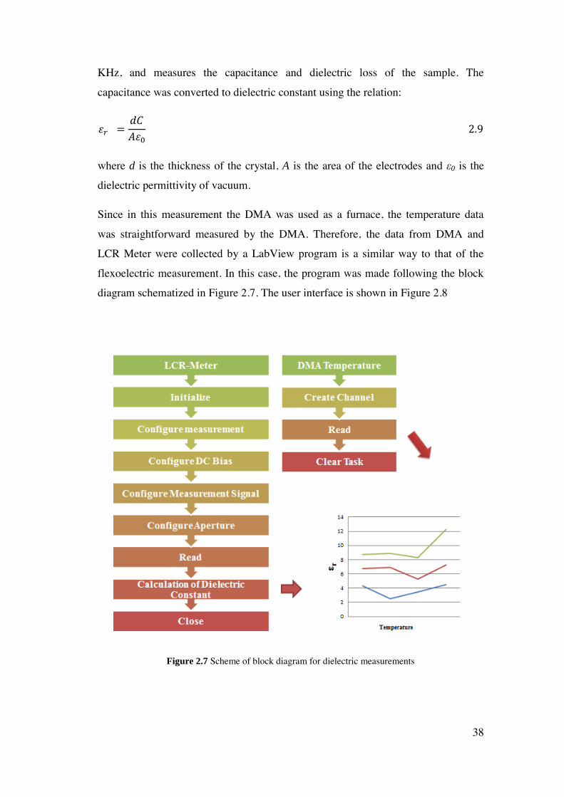
38

KHz, and measures the capacitance and dielectric loss of the sample. The

capacitance was converted to dielectric constant using the relation:

휀𝑟 =𝑑𝐶

𝐴휀0 2.9

where d is the thickness of the crystal, A is the area of the electrodes and ε0 is the

dielectric permittivity of vacuum.

Since in this measurement the DMA was used as a furnace, the temperature data

was straightforward measured by the DMA. Therefore, the data from DMA and

LCR Meter were collected by a LabView program is a similar way to that of the

flexoelectric measurement. In this case, the program was made following the block

diagram schematized in Figure 2.7. The user interface is shown in Figure 2.8

Figure 2.7 Scheme of block diagram for dielectric measurements

39

Figure 2.8 Interface user of LabView program for dielectric measurements

2.4 SAMPLES

All samples are rectangular bars, usually with a width around 1.5mm, a length more

than 9mm and a thickness of 0.5mm.

In order to perform the flexoelectric characterization, it was essential to place

rectangular electrodes on the top and bottom surfaces as illustrated in Figure 2.9.

It is important to achieve intimate contact between electrodes and surfaces, because

otherwise air gaps or impurities can affect the measurements. Gold and platinum

electrodes were deposited on the single crystals. Top and bottom electrodes were

applied using:

Electron Beam evaporation

Pulsed Laser Deposition (PLD)

Even both techniques were used, we noticed that the PLD technique offered a better

adhesion of the electrode with the materials, thus giving better stability for the

40

measurements. Eventually, we settled with PLD deposition (at room temperature

and in vacuum) as the standard for most of our electrodes

Eventually, platinum wires of 0.05 mm in diameter were attached to the electrodes

using very small drops of silver paste as illustrated in Figure 2.9. These wires

facilitate connection of the electrodes to the internal DMA wires for flexoelectric

and capacitance measurements respectively.

2.4.1 ELECTRON BEAM EVAPORATION (E-BEAM EVAPORATION)

Electron beam evaporation (Figure 2.10) is a technique in which a target material is

exposed to an electron beam arising from the application of a huge voltage between

the sample (used as the anode) and a filament under high vacuum conditions. The

electron beam causes atoms from the source material to evaporate into the gaseous

phase. These atoms then precipitate into solid form, coating all the present surfaces

in the vacuum chamber with a thin layer of the anode material. A clear advantage of

this process is that it allows for direct transfer of energy to the target through the

induced heating and is very efficient in depositing pure evaporated material onto the

substrate. Also, the deposition rate in this process can be as low as 1nm per minute

or as high as few micrometers per minute. The efficiency in material use is high as

t

l

w

Single Crystal

Pt electrode Pt wire

Figure 2.9 Geometry of samples

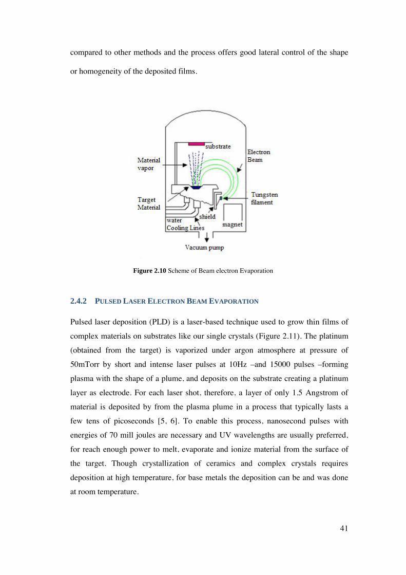
41

compared to other methods and the process offers good lateral control of the shape

or homogeneity of the deposited films.

Figure 2.10 Scheme of Beam electron Evaporation

2.4.2 PULSED LASER ELECTRON BEAM EVAPORATION

Pulsed laser deposition (PLD) is a laser-based technique used to grow thin films of

complex materials on substrates like our single crystals (Figure 2.11). The platinum

(obtained from the target) is vaporized under argon atmosphere at pressure of

50mTorr by short and intense laser pulses at 10Hz –and 15000 pulses –forming

plasma with the shape of a plume, and deposits on the substrate creating a platinum

layer as electrode. For each laser shot, therefore, a layer of only 1.5 Angstrom of

material is deposited by from the plasma plume in a process that typically lasts a

few tens of picoseconds [5, 6]. To enable this process, nanosecond pulses with

energies of 70 mill joules are necessary and UV wavelengths are usually preferred,

for reach enough power to melt, evaporate and ionize material from the surface of

the target. Though crystallization of ceramics and complex crystals requires

deposition at high temperature, for base metals the deposition can be and was done

at room temperature.

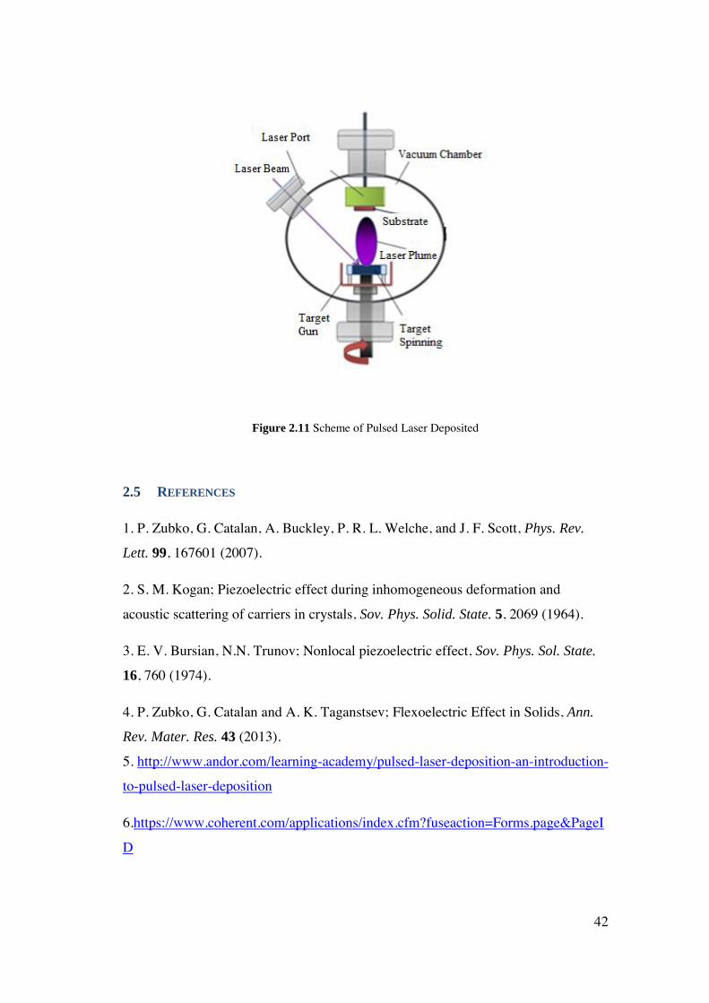
42

Figure 2.11 Scheme of Pulsed Laser Deposited

2.5 REFERENCES

1. P. Zubko, G. Catalan, A. Buckley, P. R. L. Welche, and J. F. Scott, Phys. Rev.

Lett. 99, 167601 (2007).

2. S. M. Kogan; Piezoelectric effect during inhomogeneous deformation and

acoustic scattering of carriers in crystals, Sov. Phys. Solid. State. 5, 2069 (1964).

3. E. V. Bursian, N.N. Trunov; Nonlocal piezoelectric effect, Sov. Phys. Sol. State.

16, 760 (1974).

4. P. Zubko, G. Catalan and A. K. Taganstsev; Flexoelectric Effect in Solids, Ann.

Rev. Mater. Res. 43 (2013).

5. http://www.andor.com/learning-academy/pulsed-laser-deposition-an-introduction-

to-pulsed-laser-deposition

6.https://www.coherent.com/applications/index.cfm?fuseaction=Forms.page&PageI

D

http://www.andor.com/learning-academy/pulsed-laser-deposition-an-introduction-to-pulsed-laser-deposition

http://www.andor.com/learning-academy/pulsed-laser-deposition-an-introduction-to-pulsed-laser-deposition

https://www.coherent.com/applications/index.cfm?fuseaction=Forms.page&PageID

https://www.coherent.com/applications/index.cfm?fuseaction=Forms.page&PageID

43

3 FLEXOELECTRICITY OF RELAXOR

FERROELECTRIC PMN-PT

44

3.1 INTRODUCTION.

The solid solutions formed between classical relaxor ferroelectrics such as lead

magnesium niobate PbMg1/3Nb2/3O3 (PMN) and the archetypal ferroelectric lead

titanate PbTiO3 (PT), i.e (1-x)PbMg1/3Nb2/3O3-xPbTiO3 (PMN-PT), have recently

become one of the most intensively studied materials within solid state physics, due

to their excellent piezoelectric and electromechanical properties as well the

complexity and subtlety of its phase diagram and the various length scales involved

in the structural and functional behavior of these materials.[1, 2, 3]

Relaxor ferroelectrics (relaxors) form a special class of ferroelectric materials. They

have been extensively studied both experimentally and theoretically since the 1950s

[4-7]. Relaxors are distinguished from the normal ferroelectrics by a few

characteristic features [1, 8]:

Relaxor exhibit a very broad peak of dielectric permittivity (T), often referred

as a diffuse phase transition. The temperature of maximum (T) , called Tm, is

strongly frequency dependent; namely, it shifts to higher temperatures with

increasing frequencies. Below Tm, relaxors show a very strong dielectric

dispersion. In contrast, the normal ferroelectrics exhibit a sharp, frequency

independent peak of (T) at the Curie temperature (Tc). The examples of

characteristic dielectric responses for relaxor and ferroelectric materials are

shown in Figure 3.1.

The temperature dependence of ’ in the case of normal ferroelectrics obeys the

Curie-Weiss law, as show in Figure 3.1.

휀𝑟 =𝐶

𝑇 − 𝑇0 3.1

Where C is the Curie constant and T0 is the Curie temperature. In contrast the

relaxors show strong deviations from this law above Tm. The linear dependence

of 1/’ Vs. T is obtained only at very high temperatures in relaxors, often

hundreds of degrees above Tm.

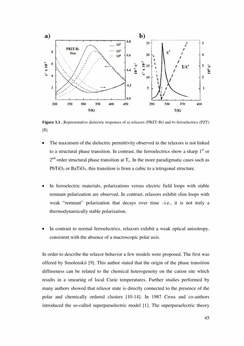
45

Figure 3.1 . Representative dielectric responses of a) relaxors (PBZT-Bi) and b) ferroelectrics (PZT)

[8]

The maximum of the dielectric permittivity observed in the relaxors is not linked

to a structural phase transition. In contrast, the ferroelectrics show a sharp 1st or

2nd order structural phase transition at Tc. In the more paradigmatic cases such as

PbTiO3 or BaTiO3, this transition is from a cubic to a tetragonal structure.

In ferroelectric materials, polarizations versus electric field loops with stable

remnant polarization are observed. In contrast, relaxors exhibit slim loops with

weak “remnant” polarization that decays over time –i.e., it is not truly a

thermodynamically stable polarization.

In contrast to normal ferroelectrics, relaxors exhibit a weak optical anisotropy,

consistent with the absence of a macroscopic polar axis.

In order to describe the relaxor behavior a few models were proposed. The first was

offered by Smolenskii [9]. This author stated that the origin of the phase transition

diffuseness can be related to the chemical heterogeneity on the cation site which

results in a smearing of local Curie temperatures. Further studies performed by

many authors showed that relaxor state is directly connected to the presence of the

polar and chemically ordered clusters [10-14]. In 1987 Cross and co-authors

introduced the so-called superparaelectric model [1]. The superparaelectric theory

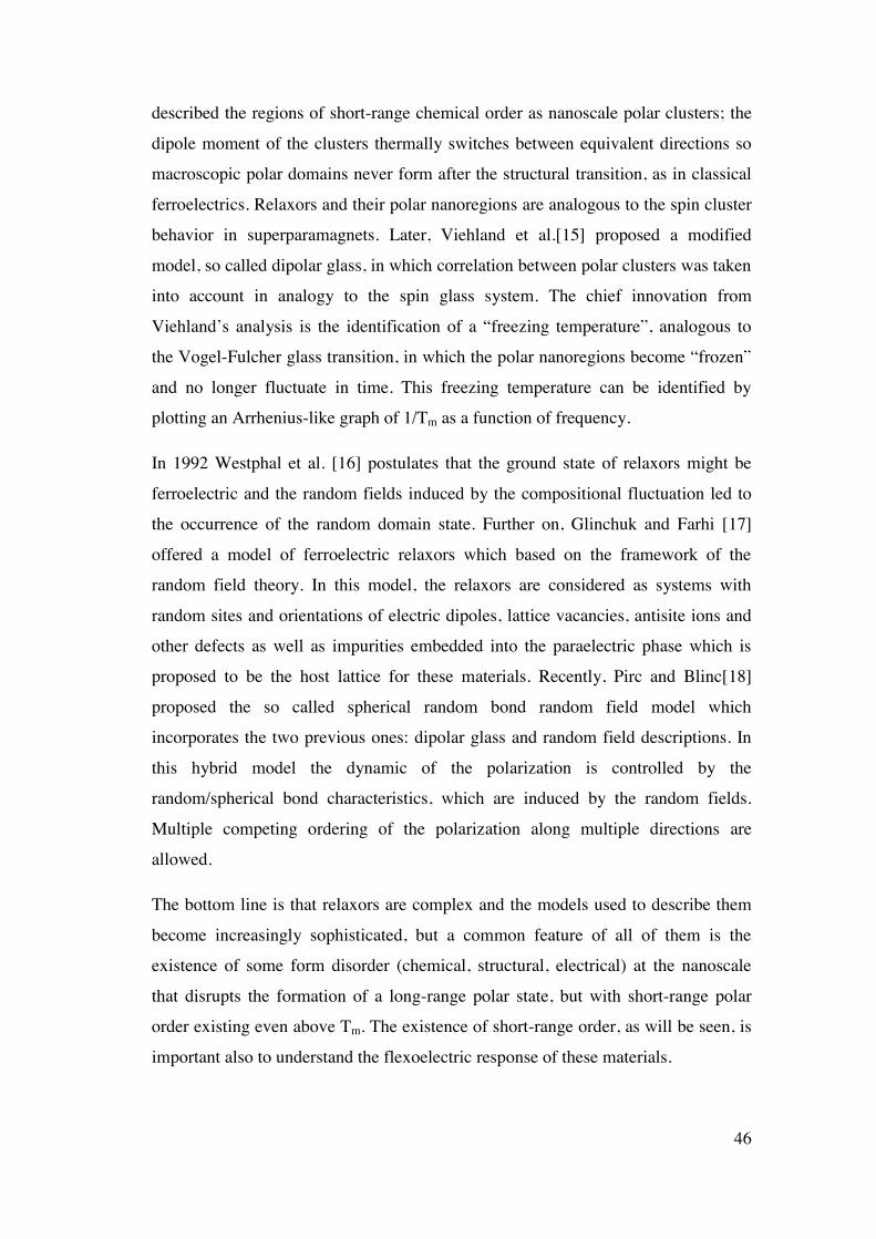
46

described the regions of short-range chemical order as nanoscale polar clusters; the

dipole moment of the clusters thermally switches between equivalent directions so

macroscopic polar domains never form after the structural transition, as in classical

ferroelectrics. Relaxors and their polar nanoregions are analogous to the spin cluster

behavior in superparamagnets. Later, Viehland et al.[15] proposed a modified

model, so called dipolar glass, in which correlation between polar clusters was taken

into account in analogy to the spin glass system. The chief innovation from

Viehland’s analysis is the identification of a “freezing temperature”, analogous to

the Vogel-Fulcher glass transition, in which the polar nanoregions become “frozen”

and no longer fluctuate in time. This freezing temperature can be identified by

plotting an Arrhenius-like graph of 1/Tm as a function of frequency.

In 1992 Westphal et al. [16] postulates that the ground state of relaxors might be

ferroelectric and the random fields induced by the compositional fluctuation led to

the occurrence of the random domain state. Further on, Glinchuk and Farhi [17]

offered a model of ferroelectric relaxors which based on the framework of the

random field theory. In this model, the relaxors are considered as systems with

random sites and orientations of electric dipoles, lattice vacancies, antisite ions and

other defects as well as impurities embedded into the paraelectric phase which is

proposed to be the host lattice for these materials. Recently, Pirc and Blinc[18]

proposed the so called spherical random bond random field model which

incorporates the two previous ones: dipolar glass and random field descriptions. In

this hybrid model the dynamic of the polarization is controlled by the

random/spherical bond characteristics, which are induced by the random fields.

Multiple competing ordering of the polarization along multiple directions are

allowed.

The bottom line is that relaxors are complex and the models used to describe them

become increasingly sophisticated, but a common feature of all of them is the

existence of some form disorder (chemical, structural, electrical) at the nanoscale

that disrupts the formation of a long-range polar state, but with short-range polar

order existing even above Tm. The existence of short-range order, as will be seen, is

important also to understand the flexoelectric response of these materials.

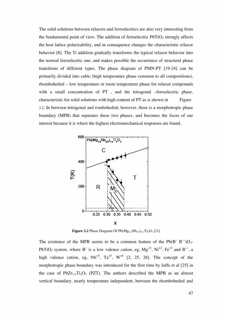
47

The solid solutions between relaxors and ferroelectrics are also very interesting from

the fundamental point of view. The addition of ferroelectric PbTiO3 strongly affects

the host lattice polarizability, and in consequence changes the characteristic relaxor

behavior [8]. The Ti addition gradually transforms the typical relaxor behavior into

the normal ferroelectric one, and makes possible the occurrence of structural phase

transitions of different types. The phase diagram of PMN-PT [19-24] can be

primarily divided into cubic (high temperature phase common to all compositions),

rhombohedral – low temperature or room temperature phase for relaxor compounds

with a small concentration of PT , and the tetragonal –ferroelectric phase,

characteristic for solid solutions with high content of PT as is shown in Figure

3.2. In between tetragonal and rombohedral, however, there is a morphotropic phase

boundary (MPB) that separates these two phases, and becomes the focus of our

interest because it is where the highest electromechanical responses are found.

Figure 3.2 Phase Diagram Of Pb(Mg1/3Nb2/3)1-xTixO3 [21]

The existence of the MPB seems to be a common feature of the Pb(B’ B’’)O3-

PbTiO3 system, where B’ is a low valence cation, eg, Mg+2, Ni+2, Fe+3 and B’’, a

high valence cation, eg, Nb+5, Ta+5, W+6 [2, 25, 26]. The concept of the

morphotropic phase boundary was introduced for the first time by Jaffe et al [25] in

the case of PbZr1-xTixO3 (PZT). The authors described the MPB as an almost

vertical boundary, nearly temperature independent, between the rhombohedral and

48

tetragonal phases. However, the MPB is now considered rather as a region in which

low symmetry phases, i.e. monoclinic or orthorhombic are present [21, 27, 28].

These low symmetry phases act as structural bridges between the tetragonal and

rhombohedral ends of the phase diagram, and enable a continuous rotation of

polarization between them, thus resulting in an enhanced piezoelectric response. The

easy polar rotation is also important to understand the flexoelectric response of these

materials, as we will see.

The giant electromechanical performance of relaxor-based ferroelectrics [29] and

the complex physics associated with their inherently nanoscopic phase separation

have inspired much research into these compounds [30]. The archetypal relaxor,

Pb(Mg1/3Nb2/3)O3 (PMN), was also the first ceramic for which bending-induced

polarization (flexoelectricity) [31, 32] was ever measured [33] and it was the

unexpectedly large value of its flexoelectric coefficient that triggered the

investigation of flexoelectricity in other perovskite ferroelectrics such as

Pb(Zr,Ti)O3[34, 35], BaTiO3 [36], and (Ba,Sr)TiO3 [37]; these investigations,

together with the realization that very large flexoelectric effects can be achieved in

the nanoscale [38-40], are ultimately behind the current surge of interest in this

phenomenon [41].

Yet, for all the research, we still do not know something as basic as the intrinsic

value of the effective flexoelectric coefficients—the constants of proportionality

between strain gradient and induced polarization. With the exception of SrTiO3 [42],

in fact, the experimentally measured flexoelectricity of most perovskites exceeds

theoretical expectations by between one and three orders of magnitude [43-46]. And

differences are not merely between theory and experiment: experimental results can

also substantially disagree among themselves. In Pb(Mg1/3Nb2/3)O3-10%PbTiO3, for

example, there is a discrepancy of three orders of magnitude between flexoelectric

coefficients measured by two different methods [47]. Meanwhile, the expected

contribution of polar nanoregions to the flexoelectricity of relaxor ferroelectrics [31]

has not been established.

Before this investigation, in fact, there were no measurements for compositions at or

near the morphotropic phase boundary either, even though their otherwise record-

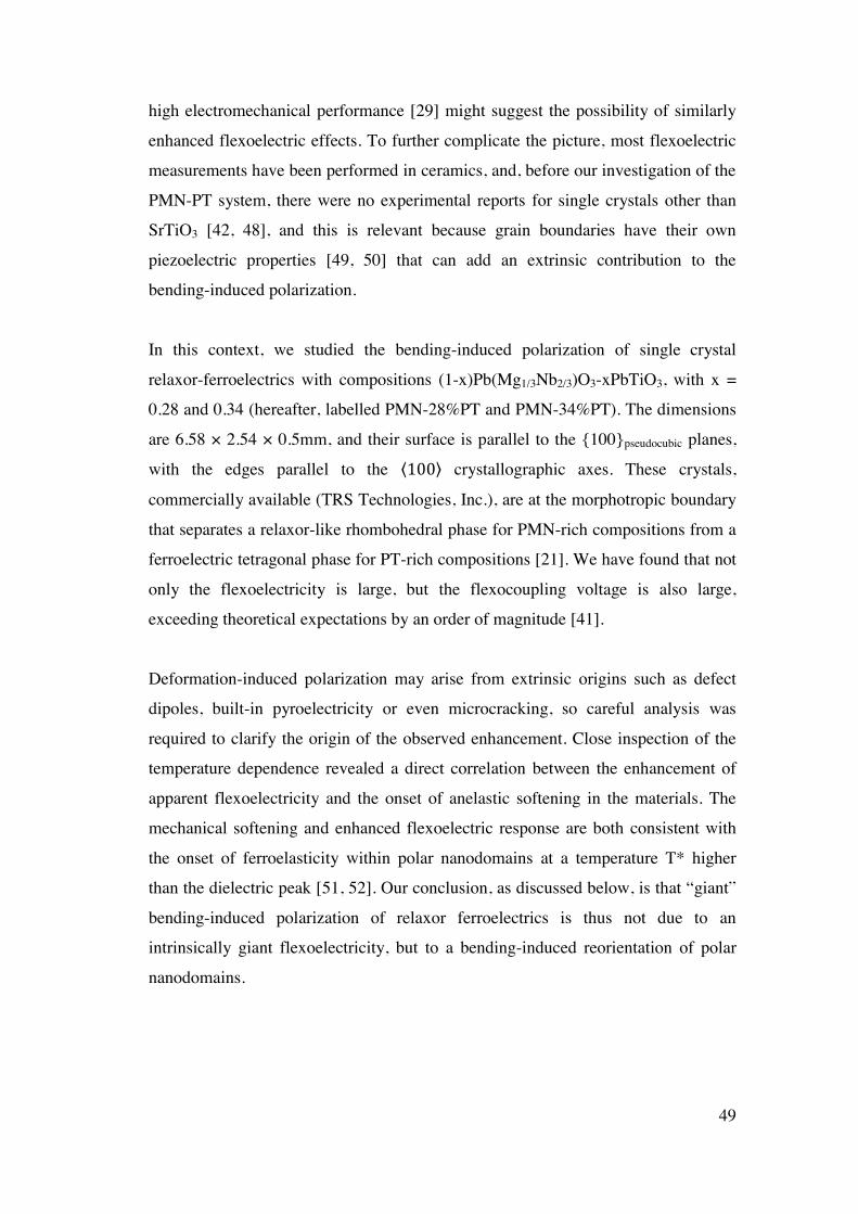
49

high electromechanical performance [29] might suggest the possibility of similarly

enhanced flexoelectric effects. To further complicate the picture, most flexoelectric

measurements have been performed in ceramics, and, before our investigation of the

PMN-PT system, there were no experimental reports for single crystals other than

SrTiO3 [42, 48], and this is relevant because grain boundaries have their own

piezoelectric properties [49, 50] that can add an extrinsic contribution to the

bending-induced polarization.

In this context, we studied the bending-induced polarization of single crystal

relaxor-ferroelectrics with compositions (1-x)Pb(Mg1/3Nb2/3)O3-xPbTiO3, with x =

0.28 and 0.34 (hereafter, labelled PMN-28%PT and PMN-34%PT). The dimensions

are 6.58 × 2.54 × 0.5mm, and their surface is parallel to the {100}pseudocubic planes,

with the edges parallel to the ⟨100⟩ crystallographic axes. These crystals,

commercially available (TRS Technologies, Inc.), are at the morphotropic boundary

that separates a relaxor-like rhombohedral phase for PMN-rich compositions from a

ferroelectric tetragonal phase for PT-rich compositions [21]. We have found that not

only the flexoelectricity is large, but the flexocoupling voltage is also large,

exceeding theoretical expectations by an order of magnitude [41].

Deformation-induced polarization may arise from extrinsic origins such as defect

dipoles, built-in pyroelectricity or even microcracking, so careful analysis was

required to clarify the origin of the observed enhancement. Close inspection of the

temperature dependence revealed a direct correlation between the enhancement of

apparent flexoelectricity and the onset of anelastic softening in the materials. The

mechanical softening and enhanced flexoelectric response are both consistent with

the onset of ferroelasticity within polar nanodomains at a temperature T* higher

than the dielectric peak [51, 52]. Our conclusion, as discussed below, is that “giant”

bending-induced polarization of relaxor ferroelectrics is thus not due to an

intrinsically giant flexoelectricity, but to a bending-induced reorientation of polar

nanodomains.

50

3.2 DIELECTRIC CHARACTIZATION OF (1-X)PMN-XPT.

As discussed at the introduction, flexoelectricity is proportional to dielectric

permittivity [31, 32, 41, 54], so it is useful to start by characterizing the dielectric

constant of the crystals. The dielectric constant and loss as a function of temperature

(Figure 3.3) have been measured at 1 kHz. The heating and cooling ramps were

identical to those of the flexoelectric measurements (3 K/min). The dielectric losses

are low (tan d<0.05) for both samples throughout the entire temperature range of the

experiments: this ensures that the impedance response is predominantly dielectric

even at the highest recorded temperatures, where dielectric losses start to rise due to

increased conductivity.

Both samples display a clear dielectric maximum, but with differences: the peak of

PMN-34%PT is sharper and at higher temperature than that of PMN-28%PT. This is

to be expected and it correlates directly with the concentration of PbTiO3 (PT),

which is a standard ferroelectric with a high Curie temperature (TC = 492ºC) [55]:

PMN-34%PT has a dielectric response closer to that of standard ferroelectric

PbTiO3 (sharp peak and a higher Curie temperature TC = 150 ºC) while the PMN-

28%PT sample has response closer to that of conventional relaxor

Pb(Mn1/2Nb2/3)O3, with increased diffuseness and broad maximum at a lower

temperature (Tm = 125 ºC).

Although PMN-34%PT is more ferroelectric-like and PMN-28%PT more relaxor-

like, the inverse permittivity (inset of Figure 3.3) departs from linear Curie-Weiss

behavior below T* ~ 250 ºC for both compositions. Such departure is interpreted as

an indicator of the existence of polar nanoregions or polarization fluctuations,

characteristic of relaxors [56]. Thus, irrespective of whether the transition is diffuse

or sharp, the high temperature phase is relaxor-like for both PMN-28%PT and

PMN-34%PT. Transitions from a high temperature relaxor-like phase to a long-

range ferroelectric phase are typical for compositions near the boundary between the

two states [21].

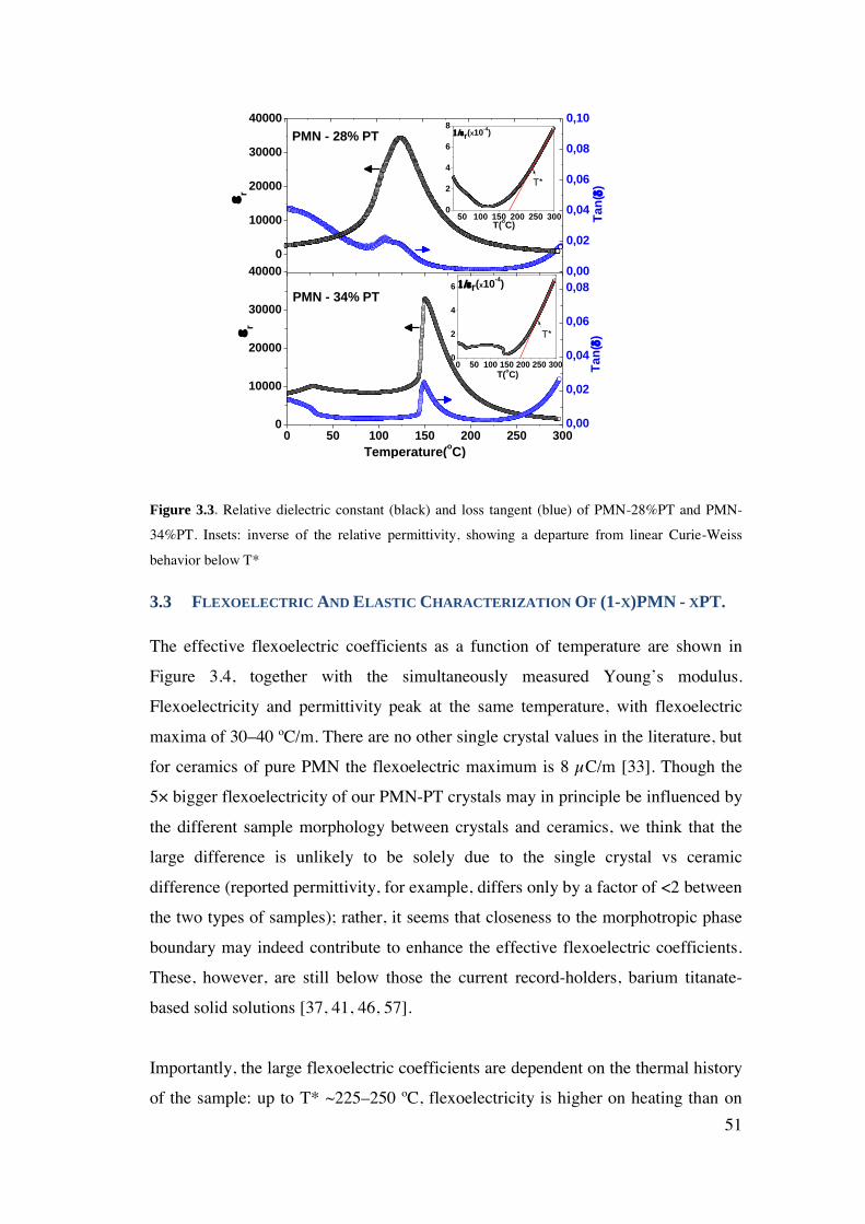
51

0 50 100 150 200 250 3000

10000

20000

30000

40000

0 50 100 150 200 250 3000

2

4

6

T(oC)

r(x10-4)

PMN - 34% PT

Temperature(oC)

T*

0

10000

20000

30000

40000

PMN - 28% PT

T*

0,00

0,02

0,04

0,06

0,08

0,00

0,02

0,04

0,06

0,08

0,10

r

r

50 100 150 200 250 3000

2

4

6

8

T(oC)

r(x10-4)

Ta

n(

)T

an

()

Figure 3.3. Relative dielectric constant (black) and loss tangent (blue) of PMN-28%PT and PMN-

34%PT. Insets: inverse of the relative permittivity, showing a departure from linear Curie-Weiss

behavior below T*

3.3 FLEXOELECTRIC AND ELASTIC CHARACTERIZATION OF (1-X)PMN - XPT.

The effective flexoelectric coefficients as a function of temperature are shown in

Figure 3.4, together with the simultaneously measured Young’s modulus.

Flexoelectricity and permittivity peak at the same temperature, with flexoelectric

maxima of 30–40 ºC/m. There are no other single crystal values in the literature, but

for ceramics of pure PMN the flexoelectric maximum is 8 µC/m [33]. Though the

5× bigger flexoelectricity of our PMN-PT crystals may in principle be influenced by

the different sample morphology between crystals and ceramics, we think that the

large difference is unlikely to be solely due to the single crystal vs ceramic

difference (reported permittivity, for example, differs only by a factor of <2 between

the two types of samples); rather, it seems that closeness to the morphotropic phase

boundary may indeed contribute to enhance the effective flexoelectric coefficients.

These, however, are still below those the current record-holders, barium titanate-

based solid solutions [37, 41, 46, 57].

Importantly, the large flexoelectric coefficients are dependent on the thermal history

of the sample: up to T* ~225–250 ºC, flexoelectricity is higher on heating than on

52

cooling, and this suggests a presence and participation of domains. The thermal

hysteresis is more pronounced in PMN-28%PT, which is also consistent with bigger

fraction metastable domains in the more relaxor-like compound.

0 50 100 150 200 250 300

30

40

50

60

70

80

90

E (

GP

a)

Temperature (oC)

0 50 100 150 200 250 300

20

30

40

50

60

70

E

(G

Pa)

0

10

20

30

40

PMN - 34% PT

Temperature (oC)

13

eff (

C/m

)

0

10

20

30

40

T* T*

PMN - 28% PT

13

eff (

C/m

)

Figure 3.4 Temperature dependence of the flexoelectric coefficients and elastic Young’s modulus of

PMN-28%PT and PMN-34%PT.

Further evidence for the participation of domains comes from analysis of the elastic

behavior in Figure 3.4 At high temperatures, the Young’s modulus E is relatively

constant, but around 200–250 ºC the lattice begins to soften, with the Young’s

modulus decreasing from 60GPa above T* to 20GPa below Tm for PMN-28%PT,

and from 80GPa to 40GPa for PMN-34%PT. This softening is anelastic, as indicated

by the increase in mechanical losses and a classic indication of the onset of

ferroelastic domain activity, with the twin wall motion being both a way to relax the

stress and a mechanical energy dissipation mechanism.

3.4 FLEXOCOUPLING CHARACTERIZATION OF (1-X)PMN-XPT.

In order to gain further insight into the high values of flexoelectricity, we now

examine the flexoelectric coefficient normalized by the dielectric constant (Figure

3.5). Theoretically, this so-called flexo-coupling (or flexo-voltage [40]) coefficient,

f, should be of the order of 1–10 V[41]. Experimentally, instead, the measured

53

coefficients reach up to f ~100–300 V, an order of magnitude bigger than the

theoretical upper limit.

At low temperatures (i.e., below the Curie temperature), some or most of the

bending-induced polarization may be attributed to piezoelectricity. In PMN-34%PT,

long range polarization appears at TC = Tm = 150 ºC. In PMN-28%PT, which is

more relaxor-like, spontaneous long range order does not appear at any critical

temperature, and the flexocoupling coefficient grows continuously upon cooling. On

heating, though, a residual anomaly appears around Tf =100ºC < Tm =125ºC, which

we interpret as the relaxor freezing temperature below which stable polarization and

thus piezoelectricity can appear.

At temperatures above T*, however, the flexocoupling coefficient goes down to a

stable value f ≤ 10V that is not hysteretic, is constant with temperature, and is

consistent with theoretical expectations. This is therefore likely to be the true

intrinsic value of the flexocoupling coefficient.

Figure 3.5 Flexocoupling coefficients of PMN-28%PT and PMN-34%PT

54

3.5 DISCUSSION

Relaxor ferroelectrics are known to display a peak in acoustic emission at a

relatively composition-independent temperature T*~ 500 ± 30K [24, 25]. Acoustic

emission is caused by a sudden release of elastic energy, so T* must signal an elastic

discontinuity, in perfect agreement with our results and also with analysis of

resonant ultrasound spectroscopy made by Carpenter et al. [58].

The origin of the peak in acoustic emission and of mechanical anelastic softening

below T* is attributed to a ferroelastic transition within the relaxor polar

nanoregions. These regions are known to appear at a higher temperature, the so-

called Burns temperature (Tb ≥ 600K [52]) but only become ferroelastically active

at T* ~ 500K [51, 52, 58, 59]. The exitence of nanodomains is also, as discussed

before, consistent with the thermal history dependence of the bending-induced

polarization, which is higher on heating than on cooling, indicative of a bigger

volume fraction of nanodomains when heating from the ferroelectric polar state than

when cooling from the non-polar paraphase.

The appearance and subsequent growth of nanotwins below T* has consequences

for the electromechanical response of the material, because external stress can cause

a ferroelastic reorientation of the nanodomains. Under bending stress, local

compression of the x-y plane at the concave side will increase the proportion of

domains with perpendicular polarization. The bending strains reach a maximum of

ϵ11 ~ (near the center of curvature) at the surface; multiplied by the Young’s

modulus of PMN-PT (20–80 GPa), this is equivalent to a stress of 2–8 MPa, which

is sufficient to cause ferroelastic switching[25] . However, an electric bias is still

necessary in order to remove the degeneracy between the +z and -z directions:[25]

though stress can rearrange ferroelastic domains and locally favour vertical

polarization, the coupling is to the square of polarization (electrostriction) and thus

it cannot favour one polarity over its opposite [40, 41]; this is the reason why

mechanically assisted poling is always done in the presence of an electric bias[60].

Since we are not applying any external voltage in our experiments, and the

electrodes are symmetric, the biasing may be provided by the flexoelectric field,

although recent experiments by the group of Damjanovic suggest that another

55

potential source of bias may also be defect gradients, which are inherent in all

crystals even when they are nominally centrosymmetric [61]. The average strain

gradient in the bent crystals is of the order of 𝜕𝜖11

𝜕𝑧

= 0.2 m-1, and the intrinsic (high

temperature) flexocoupling coefficient is of the order of f ~ 10 V, so the equivalent

flexoelectric field is of the order of E = f 𝜕𝜖11

𝜕𝑧

= 2 V/m. This is too small compared to

typical coercive fields in ferroelectrics (kV/cm), so it is clear that the flexoelectric

field by itself cannot cause switching; at most, as discussed, it provides a

background bias that favours one polarity over the other when the polarization is

ferroelastically switched. Ferroelasticity and flexoelectricity must therefore work in

tandem to achieve the enhancement: the first causes the switching, and the second

dictates the polarity of the switched state. Defect gradients may of course also cause

a similar bias, but in that case it will probably be active only for a given orientation

of the crystal and not for the opposite, as we discuss in the next chapter.

The effective flexoelectricity caused by this cooperative “flexoferroelastic”

switching is not bound by the Kogan-Tagantsev limit and can therefore yield

domain-based effective flexocoupling coefficients orders of magnitude larger than

the intrinsic lattice-based flexoelectricity, which we have measured as an almost

constant f13=10V above T*. Though the potential practical usefulness of giant

flexoelectricity for electromechanical transduction is mostly unaffected by its origin,

the small thermal hysteresis, typical of domain-based properties, is undesirable and

should be minimized.

Perhaps more importantly, these results are evidence that giant bending-induced

polarization can be obtained without an intrinsically giant flexoelectricity, and this

observation is a first step towards reconciling some of the discrepancies about the

true magnitude of the flexoelectric coefficient. In the next chapter, we will see that

nanodomain contribution to effective flexoelectricity is a pervasive phenomenon

that affects not only relaxors but also very standard ferroelectrics, and we will also

see that there is at least another source of bending-induced polarization that further

modifies the intrinsic bulk value; namely, surface piezoelectricity.

56

3.6 REFERENCES.

1. L.E. Cross, Ferroelectrics 76, 241 (1987)

2. J. Kuwata, K. Uchino and S. Nomura, Ferroelectrics 37, 579 (1981)

3. J. Kuwata, K. Uchino and S. Nomura, Jpn. J. Appl. Phys. 21, 1298 (1982)

4. G. Shirane and A. Takeda, J. Phys. Soc. Jpn. 7, 5 (1952)

5. G. Shirane and K. Suzuki, J. Phys. Soc. Jpn. 7, 333 (1952)

6. G. A. Smolenskii and A. I. Agranovskaya, Sov. Phys. Tech. Phys. 3, 1380 (1958)

7. V. A. Bokov and I. E. Mylnikova, Fiz. Tverd. Tela 2, 2728 (1960)

8. G. A. Samara, J. Phys.: Condens. Matter 15, R367 (2003)

9. G. A. Smolenskii, J. Phys. Soc. Jpn. 28, 26 (1970)

10. G. Burns and B. A. Scott, Solid State Commun. 13, 417 (1973)

11. N. A. Setter and L. E. Cross, J. Appl. Phys. 51, 4356 (1980)

12. C. G. Stenger and A. F. Burgraaf, Phys. Status Solidi (a) 61, 275, (1980)

13. G. Burns and F. H. Dacol, Phys. Rev. B 28, 2527 (1983)

14. X. Yao, Z. L. Chen and L. E. Cross, J. Appl. Phys. 54, 3399 (1984)

15. D. Viehland, S. J. Jang, L. E. Cross and M. Wutting, J. Appl. Phys. 68, 2916

(1990)

16. V. Westphal, W. Kleemann and M. D. Glinchuk, Phys. Rev. Lett. 68, 847 (1992)

17. M. D. Glinchuk and R. Fahri, J. Phys.: Condens. Matter 8, 6985 (1996)

18. R. Pirc and R. Blinc, Phys. Rev. B 60, 13470 (1999)

19. W. Choi, T.R. Shrout, S. J. Jang and A.S. Bhalla, Ferroelectrics 100, 29 (1989)

20. O. Noblanc, P. Gaucher and G. Calvarin, J. Appl. Phys. 79, 4291 (1996)

57

21. B. Noheda, D. E. Cox, G. Shirane, Z.-G. Ye and J. Gao, Phys. Rev. B. 66,

054104 (2002)

22. P. M. Gehring, W. Chen, Z. G. Ye and G. Shirane, J. Phys.: Condens. Matter.

16, 7113 (2004)

23. D. Zekria, V. A. Shuvaeva and A. M. Glazer, J. Phys.: Condens. Matter 17,

1593(2005)

24. V. A. Shuvaeva, A. M. Glazer and D. Zekria, J. Phys.: Condens. Matter 17,

5709(2005)

25. B. Jaffe, W. R. Cook, and H. Jaffe, Piezoelectric ceramics (Academic Press,

London, 1971)

26. T. Shrout, Z.P. Chang, N. Kim and S. Markgraf, Ferroelectr. Lett. Sect. 12,

63(1990)

27. D. La-Orauttapong, B. Noheda, Z.-G. Ye, P. M. Gehring, J. Toulouse and D. E.

Cox, Phys. Rev. B 65, 144101 (2002)

28. B. Noheda, Curr. Opin. Solid State Mater. 6, 27 (2002)

29. S. E. Park and T. R. Shrout, J. Appl. Phys. 82, 1804–1811 (1997).

30. A. A. Bokov and Z.-G. Ye, J. Mater. Sci. 41, 31–52 (2006).

31. S. M. Kogan, Sov. Phys. Solid State. 5, 2069–2070 (1964).

32. A. K. Tagantsev, Phys. Rev. B. 34, 5883–5888 (1986).

33. W. Ma and L. E. Cross, Appl. Phys. Lett. 78, 2920–2921 (2001).





58

38. G. Catalan, L. J. Sinnamon, and J. M. Gregg, J. Phys.: Condens. Matter. 16,

2253–2264 (2004).

39. G. Catalan, A. Lubk, A. H. G. Vlooswijk, E. Snoeck, C. Magen, A. Janssens, G.

Rispens, G. Rijnders, D. H. A. Blank, and B. Noheda, Nat. Mater. 10, 963–967

(2011).

40. H. Lu, C.-W. Bark, D. Esque de los Ojos, J. Alcala, C. B. Eom, G. Catalan, and

A. Gruverman, Science. 336, 59–61 (2012).

41. P. Zubko, G. Catalan, and A. K. Tagantsev, Annu. Rev. Mater. Res. 43, 387–421

(2013).


Lett. 99, 167601 (2007).

43. R. Maranganti and P. Sharma, Phys. Rev. B. 80, 054109 (2009).

44. J. Hong, G. Catalan, J. F. Scott, and E. Artacho, J. Phys.: Condens. Matter 22,

112201 (2010).


46. L. Shu, X. Wei, L. Jin, Y. Li, H. Wang, and X. Yao, Appl. Phys. Lett. 102,

152904 (2013).

47. P. Hana, Ferroelectrics. 351, 196–203 (2007).


Lett. 100, 199906 (2008).

49. A. Kholkin, I. Bdikin, T. Ostapchuk, and J. Petzelt, Appl. Phys. Lett. 93, 222905

(2008).

50. J. Petzelt, T. Ostapchuk, I. Gregora, I. Rychetsk_y, S. Hoffmann-Eifert, A. V.

Pronin, Y. Yuzyuk, B. P. Gorshunov, S. Kamba, V. Bovtun et al., Phys. Rev. B. 64,

184111 (2001).

51. M. Roth, E. Mojaev, E. Dul’kin, P. Gemeiner, and B. Dkhil, Phys. Rev. Lett. 98,

265701 (2007).

59

52. B. Dkhil, P. Gemeiner, A. Al-Barakaty, L. Bellaiche, E. Dul’kin, E.Mojaev, and

M. Roth, Phys. Rev. B. 80, 064103 (2009).

53. M. Stengel, Phys. Rev. B 88, 174106 (2013).

54. E. V. Bursian and O. I. Zaikovskii, Sov. Phys. Solid State. 10, 1121–1124

(1968).

55. M. J. Haun, E. Furman, S. J. Jang, H. A. McKinstry, and L. E. Cross, J. Appl.

Phys. 62, 3331–3338 (1987).

56. D. Viehland, S. J. Jang, L. E. Cross, and M. Wuttig, Phys. Rev. B 46, 8003–8006

(1992)

57. L. E. Cross, J. Mater. Sci. 41, 53–63 (2006).

58. M. A. Carpenter, J. F. J. Bryson, G. Catalan, S. J. Zhang, and N. J. Donnelly, J.

Phys.: Condens. Matter. 24, 045902 (2012).

59. M. A. Carpenter, J. F. J. Bryson, G. Catalan, and C. J. Howard, J. Phys.:

Condens. Matter. 24, 045901 (2012).

60. A. E. McLaughlin, T. Liu, and S. C. Lynch, Acta Mater. 53, 4001–4008 (2005).

61. A. Biancoli, C. M. Fancher, J. L. Jones and D. Damjanovic, Nat. Mater. 14, 224-229 (2015)

60

4 FLEXOELECTRICITY OF SINGLE

CRYSTAL BATIO3

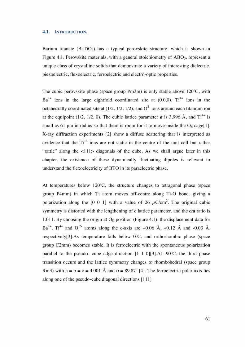
61

4.1. INTRODUCTION.

Barium titanate (BaTiO3) has a typical perovskite structure, which is shown in

Figure 4.1. Perovskite materials, with a general stoichiometry of ABO3, represent a

unique class of crystalline solids that demonstrate a variety of interesting dielectric,

piezoelectric, flexoelectric, ferroelectric and electro-optic properties.

The cubic perovskite phase (space group Pm3m) is only stable above 120ºC, with

Ba2+ ions in the large eightfold coordinated site at (0,0,0), Ti4+ ions in the

octahedrally coordinated site at (1/2, 1/2, 1/2), and O2- ions around each titanium ion

at the equipoint (1/2, 1/2, 0). The cubic lattice parameter a is 3.996 Å, and Ti4+ is

small as 61 pm in radius so that there is room for it to move inside the O6 cage[1].

X-ray diffraction experiments [2] show a diffuse scattering that is interpreted as

evidence that the Ti+4 ions are not static in the centre of the unit cell but rather

“rattle” along the <111> diagonals of the cube. As we shall argue later in this

chapter, the existence of these dynamically fluctuating dipoles is relevant to

understand the flexoelectricity of BTO in its paraelectric phase.

At temperatures below 120ºC, the structure changes to tetragonal phase (space

group P4mm) in which Ti atom moves off-centre along Ti-O bond, giving a

polarization along the [0 0 1] with a value of 26 µC/cm2. The original cubic

symmetry is distorted with the lengthening of c lattice parameter, and the c/a ratio is

1.011. By choosing the origin at OII position (Figure 4.1), the displacement data for

Ba2+, Ti4+ and OI2- atoms along the c-axis are +0.06 Å, +0.12 Å and -0.03 Å,

respectively[3].As temperature falls below 0ºC, and orthorhombic phase (space

group C2mm) becomes stable. It is ferroelectric with the spontaneous polarization

parallel to the pseudo- cube edge direction [1 1 0][3].At -90ºC, the third phase

transition occurs and the lattice symmetry changes to rhombohedral (space group

Rm3) with a = b = c = 4.001 Å and α = 89.87º [4]. The ferroelectric polar axis lies

along one of the pseudo-cube diagonal directions [111]

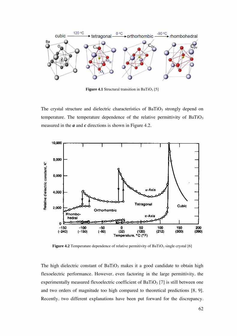
62

Figure 4.1 Structural transition in BaTiO3 [5]

The crystal structure and dielectric characteristics of BaTiO3 strongly depend on

temperature. The temperature dependence of the relative permittivity of BaTiO3

measured in the a and c directions is shown in Figure 4.2.

Figure 4.2 Temperature dependence of relative permitivity of BaTiO3 single crystal [6]

The high dielectric constant of BaTiO3 makes it a good candidate to obtain high

flexoelectric performance. However, even factoring in the large permittivity, the

experimentally measured flexoelectric coefficient of BaTiO3 [7] is still between one

and two orders of magnitude too high compared to theoretical predictions [8, 9].

Recently, two different explanations have been put forward for the discrepancy.

63

Biancoli et al. [10] have observed net polarization in nominally paraelectric SrTiO3

and (Ba,Sr)TiO3. Such built-in macroscopic polarizations are inherent to fabrication

processes and common to all materials and may therefore explain the large bending-

induced polarization of BaTiO3. In contrast, Bersuker’s theoretical analysis

concludes that the large flexoelectric response is due instead to a flexoelectrically-

induced alignment of precursor polarization that exists in the paraelectric phase of

BaTiO3 [11]. In this scenario, BaTiO3 would behave similar to relaxor ferroelectrics,

as we have described in the previous chapter [12]. The investigation on the

magnitude and origin of the enhanced flexoelectricity in BaTiO3 single crystals is

the subject of the research presented in this chapter.

In order to identify different contributions to the total bending-induced polarization,

we have studied the flexoelectricity of BaTiO3 single crystals of different orientation

in the temperature range between 25 ºC and 300 ºC. The samples were commercially

acquired from SurfaceNet and MTI crystal, and their dimensions were 10 mm long,

1mm wide and 0.5 mm thick. In order to characterize anisotropy, we examine

crystals with surfaces parallel to the (111), (110) and (001) crystallographic planes

respectively. We found that the enhancement is consistent with the existence of

precursor polarization in the paraelectric phase, but we additionally find a strong

anisotropy that cannot be a bulk effect. We attribute this anisotropy to the predicted

[13, 14] but experimentally unconfirmed contribution of surface piezoelectricity to

the total flexoelectricity of even bulk crystals.

4.2. DIELECTRIC CHARACTERIZATION OF BATIO3.

Figure 4.3 shows the dielectric constant and dielectric loss as a function of

temperature for (001), (011) and (111)-BaTiO3 oriented single crystals. A sharp peak

in dielectric constant, corresponding to the first order transition between the

paraelectric and ferroelectric phase, is observed around TC~120-125 ºC for all

samples. The cubic phase is orthotropic and the dielectric constant above TC is the

same for these three orientations, while in the ferroelectric phase (below TC) it is

sensitive to both crystal orientation and domain configuration [15]. The dielectric

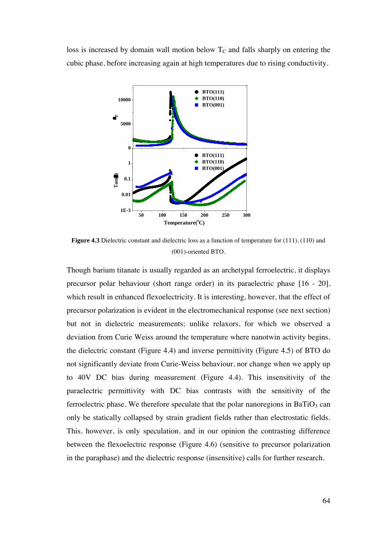
64

loss is increased by domain wall motion below TC and falls sharply on entering the

cubic phase, before increasing again at high temperatures due to rising conductivity.

50 100 150 200 250 3001E-3

0.01

0.1

1

BTO(111)

BTO(110)

BTO(001)

Temperature(oC)

0

5000

10000

BTO(111)

BTO(110)

BTO(001)

Ta

n(

) r

Figure 4.3 Dielectric constant and dielectric loss as a function of temperature for (111), (110) and

(001)-oriented BTO.

Though barium titanate is usually regarded as an archetypal ferroelectric, it displays

precursor polar behaviour (short range order) in its paraelectric phase [16 - 20],

which result in enhanced flexoelectricity. It is interesting, however, that the effect of

precursor polarization is evident in the electromechanical response (see next section)

but not in dielectric measurements; unlike relaxors, for which we observed a

deviation from Curie Weiss around the temperature where nanotwin activity begins,

the dielectric constant (Figure 4.4) and inverse permittivity (Figure 4.5) of BTO do

not significantly deviate from Curie-Weiss behaviour, nor change when we apply up

to 40V DC bias during measurement (Figure 4.4). This insensitivity of the

paraelectric permittivity with DC bias contrasts with the sensitivity of the

ferroelectric phase. We therefore speculate that the polar nanoregions in BaTiO3 can

only be statically collapsed by strain gradient fields rather than electrostatic fields.

This, however, is only speculation, and in our opinion the contrasting difference

between the flexoelectric response (Figure 4.6) (sensitive to precursor polarization

in the paraphase) and the dielectric response (insensitive) calls for further research.

65

50 100 150 200 250 3001E-7

1E-6

1E-5 DCBias = 0V

DCBias = 40V

Ca

pa

cita

nce

(F

)

Temperature(ºC)

Figure 4.4 Capacitance as a function of temperature for (001)-oriented BaTiO3 at 0V and 40V

50 100 150 200 250 300

0

5

10

15

20

25

1/

r(x1

0-4)

Temperature(ºC)

Figure 4.5 Inverse dielectric constant as a function of temperature for (001)-oriented BaTiO3

4.3. FLEXOELECTRIC CHARACTERIZATION OF BATIO3.

The effective flexoelectric coefficients are plotted in Figure 4.6. The peaks at Tc

mirror those observed in the permittivity. The maxima for the flexoelectric

coefficient are in the 10-100 µC/m range, but these values fall sharply to 1-10 C/m

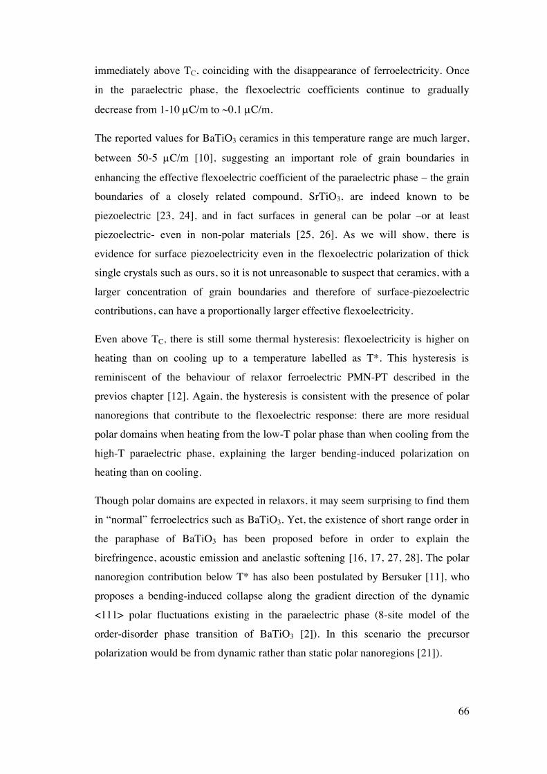
66

immediately above TC, coinciding with the disappearance of ferroelectricity. Once

in the paraelectric phase, the flexoelectric coefficients continue to gradually

decrease from 1-10 C/m to ~0.1 C/m.

The reported values for BaTiO3 ceramics in this temperature range are much larger,

between 50-5 C/m [10], suggesting an important role of grain boundaries in

enhancing the effective flexoelectric coefficient of the paraelectric phase – the grain

boundaries of a closely related compound, SrTiO3, are indeed known to be

piezoelectric [23, 24], and in fact surfaces in general can be polar –or at least

piezoelectric- even in non-polar materials [25, 26]. As we will show, there is

evidence for surface piezoelectricity even in the flexoelectric polarization of thick

single crystals such as ours, so it is not unreasonable to suspect that ceramics, with a

larger concentration of grain boundaries and therefore of surface-piezoelectric

contributions, can have a proportionally larger effective flexoelectricity.

Even above TC, there is still some thermal hysteresis: flexoelectricity is higher on

heating than on cooling up to a temperature labelled as T*. This hysteresis is

reminiscent of the behaviour of relaxor ferroelectric PMN-PT described in the

previos chapter [12]. Again, the hysteresis is consistent with the presence of polar

nanoregions that contribute to the flexoelectric response: there are more residual

polar domains when heating from the low-T polar phase than when cooling from the

high-T paraelectric phase, explaining the larger bending-induced polarization on

heating than on cooling.

Though polar domains are expected in relaxors, it may seem surprising to find them

in “normal” ferroelectrics such as BaTiO3. Yet, the existence of short range order in

the paraphase of BaTiO3 has been proposed before in order to explain the

birefringence, acoustic emission and anelastic softening [16, 17, 27, 28]. The polar

nanoregion contribution below T* has also been postulated by Bersuker [11], who

proposes a bending-induced collapse along the gradient direction of the dynamic

<111> polar fluctuations existing in the paraelectric phase (8-site model of the

order-disorder phase transition of BaTiO3 [2]). In this scenario the precursor

polarization would be from dynamic rather than static polar nanoregions [21]).

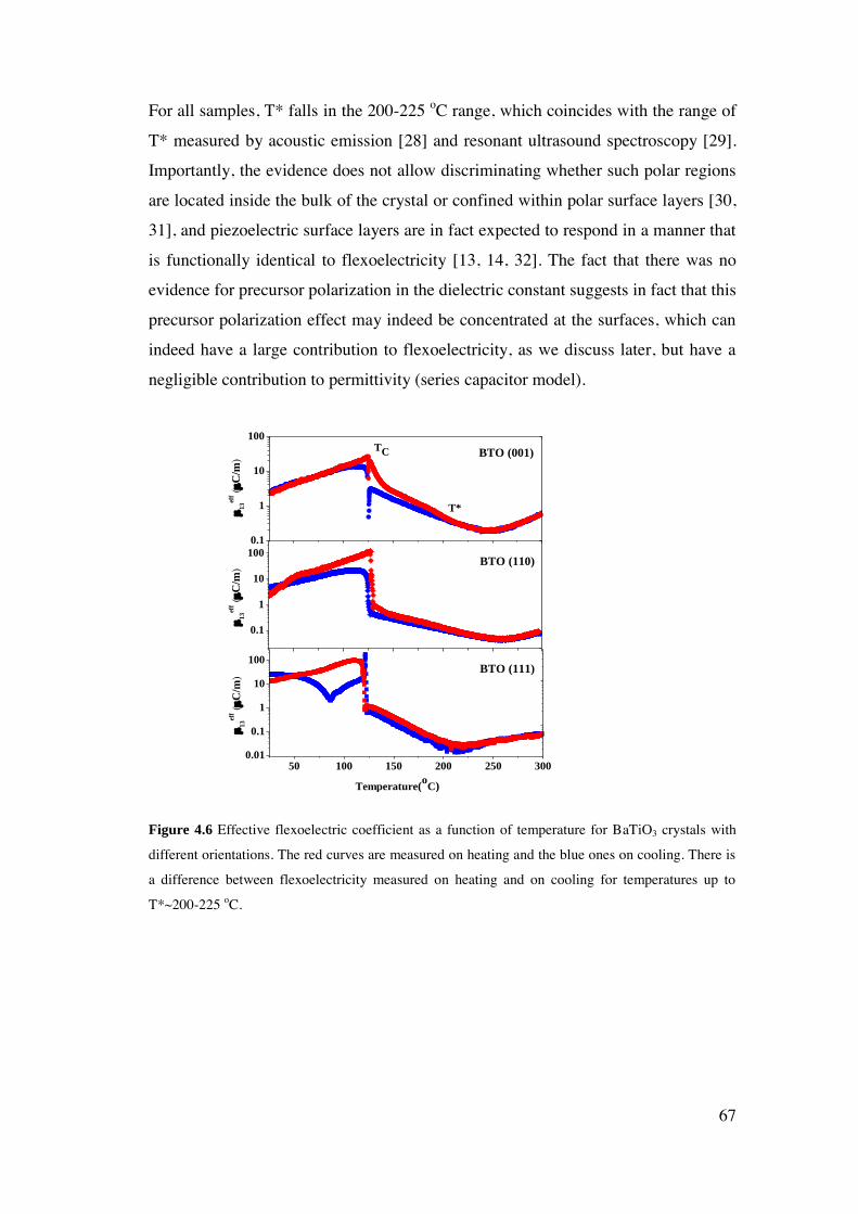
67

For all samples, T* falls in the 200-225 oC range, which coincides with the range of

T* measured by acoustic emission [28] and resonant ultrasound spectroscopy [29].

Importantly, the evidence does not allow discriminating whether such polar regions

are located inside the bulk of the crystal or confined within polar surface layers [30,

31], and piezoelectric surface layers are in fact expected to respond in a manner that

is functionally identical to flexoelectricity [13, 14, 32]. The fact that there was no

evidence for precursor polarization in the dielectric constant suggests in fact that this

precursor polarization effect may indeed be concentrated at the surfaces, which can

indeed have a large contribution to flexoelectricity, as we discuss later, but have a

negligible contribution to permittivity (series capacitor model).

50 100 150 200 250 3000.01

0.1

1

10

100

Temperature(oC)

0.1

1

10

100

BTO (111)

BTO (110)

13

eff (

C/m

)

13

eff (

C/m

)

0.1

1

10

100TC

13

eff (

C/m

)

BTO (001)

T*

Figure 4.6 Effective flexoelectric coefficient as a function of temperature for BaTiO3 crystals with

different orientations. The red curves are measured on heating and the blue ones on cooling. There is

a difference between flexoelectricity measured on heating and on cooling for temperatures up to

T*~200-225 oC.

68

4.4. FLEXOCOUPLING CHARACTERIZATION OF BATIO3.

As discussed at the introduction, the flexoelectric coefficient normalized by the

dielectric constant is known as flexocoupling (or flexovoltage) coefficient, f (Figure

4.7). Theoretically, for an intrinsic flexoelectric effect, f should be of the order of 1

< f < 20V and temperature-independent [33-36]. Experimentally, we found f to be

close to 10000V immediately below TC, but this must clearly be due to the

piezoelectric response of the ferroelectric phase and not a real flexoelectric effect;

verification of this piezoelectric origin can be found in the 180 degree phase

inversion of the low temperature signal upon turning the crystal upside down, shown

in Figure 4.8. At TC, the flexovoltage f decreases sharply (first order phase

transition), and then more gradually up to T*, consistent with the aforementioned

picture of gradual extinction of the precursor polar regions. Meanwhile, at

temperatures around 250 oC or higher, leakage currents artificially increase the

capacitance (Maxwell-Wagner model) and thus also the effective flexocoupling

again. This correlation between high leakage and flexoelectric increase is in fact the

first evidence that free charges inside a dielectric can contribute to effective

flexoelectricity, something that we explore and exploit to great advantage in the next

chapter of this thesis.

There has been a suggestion that some or all of the anomalous flexoelectric

enhancement of dielectric BaTiO3 and related compounds may be due to built-in

piezoelectricity caused by gradients in defect concentration that appear during

sample fabrication[10]. We have examined this hypothesis by looking at the phase

angle of the bending-induced current: if the polarization is piezoelectric in nature,

one would expect it to be inverted (i.e., the phase delay of the current with respect to

the strain gradient should change by 180 degrees) when the crystal is turned upside-

down. Here we must note that the absolute value of the phase angle is not

meaningful because the preamplifier circuit introduces a phase lag. The relative

change of phase, however, is robust, and a typical phase measurement is shown in

Figure 4.8. At room temperature, there is indeed a difference of 180 degrees upon

inverting the sample, consistent with the existence of a preferential macroscopic

orientation of the ferroelectric polarization. However, above TC there is no

difference between the phase angles. Any macroscopic polarization, if it exists,

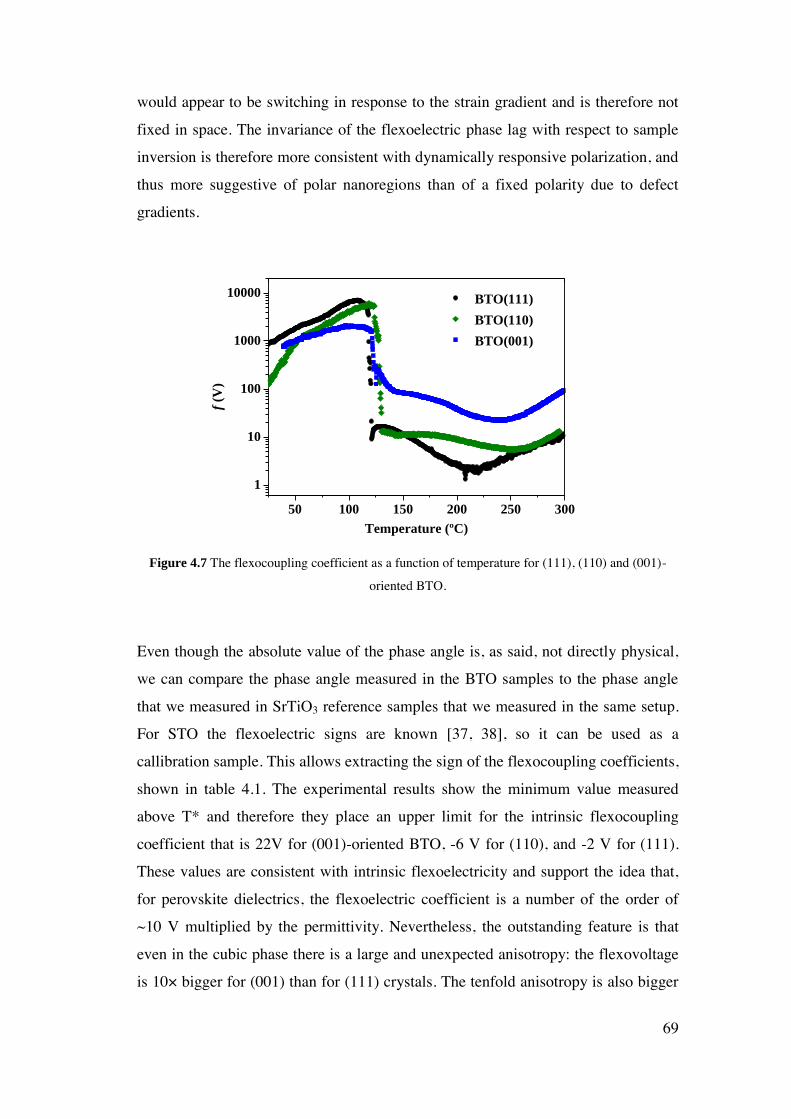
69

would appear to be switching in response to the strain gradient and is therefore not

fixed in space. The invariance of the flexoelectric phase lag with respect to sample

inversion is therefore more consistent with dynamically responsive polarization, and

thus more suggestive of polar nanoregions than of a fixed polarity due to defect

gradients.

50 100 150 200 250 300

1

10

100

1000

10000BTO(111)

BTO(110)

BTO(001)

f (V

)

Temperature (ºC)

Figure 4.7 The flexocoupling coefficient as a function of temperature for (111), (110) and (001)-

oriented BTO.

Even though the absolute value of the phase angle is, as said, not directly physical,

we can compare the phase angle measured in the BTO samples to the phase angle

that we measured in SrTiO3 reference samples that we measured in the same setup.

For STO the flexoelectric signs are known [37, 38], so it can be used as a

callibration sample. This allows extracting the sign of the flexocoupling coefficients,

shown in table 4.1. The experimental results show the minimum value measured

above T* and therefore they place an upper limit for the intrinsic flexocoupling

coefficient that is 22V for (001)-oriented BTO, -6 V for (110), and -2 V for (111).

These values are consistent with intrinsic flexoelectricity and support the idea that,

for perovskite dielectrics, the flexoelectric coefficient is a number of the order of

~10 V multiplied by the permittivity. Nevertheless, the outstanding feature is that

even in the cubic phase there is a large and unexpected anisotropy: the flexovoltage

is 10× bigger for (001) than for (111) crystals. The tenfold anisotropy is also bigger

70

than observed in homomorphic SrTiO3, for which it is a factor smaller than three.

We now turn our attention to the origin of this large anisotropy.

50 100 150 200

-180

-90

0

90

180Side 1 up

Side 1 down

eff

13 P

hase

(d

egre

es)

Temperature(°C)

Figure 4.8 Phase angle between applied force and bending-induced current for a crystal measured

twice consecutively, with its orientation flipped upside down between the two measurements. The

room-temperature polarization changes phase by 180 degrees, consistent with the existence of a net

macroscopic polarity. In contrast, above TC the phase angle between force and current is identical for

the two measurements, indicating that the flexoelectric enhancement in the paraelectric phase is not

due to macroscopic built-in polarization.

Table 4.1 shows the orientation of the sample edges with respect to the

crystallographic axes, determined using X-ray diffraction. As was previously

reported [37], the effective coefficient for any given cubic crystal orientation is

always a linear combination of the coefficients for the other two; in other words

there do not exist three independent equations required to obtain the three

independent tensor components in cubic symmetry. On the other hand, the linear

dependence provides a “sanity check”: if the measured coefficients are only

dependent on the bulk properties of the sample (i.e., if there is no surface

piezoelectricity), then the effective flexoelectric coefficient of, for example, the

(001)-oriented sample can in principle be calculated from the effective flexoelectric

coefficients measured for (111) and (011) orientations. Conversely, if the calculated

and measured values do not coincide, it is a strong indication that non-bulk

contributions must be present.

71

Table 4.1 The effective flexoelectric and flexoelectric coefficients for (100), (𝟏��𝟎) and (𝟏𝟎��)-

oriented single crystals of BaTiO3

x1 x2 x3 µ13(µC/m) f (V)

[100] [010] [001] 0.20 22

[𝟏��𝟎] [001] [110] -0.05 -6

[𝟏𝟎��] [121] [111] -0.01 -2

--------------------

Equation A.31 from the appendix relates the flexocoupling coefficient along (100)

to the flexocoupling coefficients along (110) and (111):

1.47𝑓111𝑏𝑒𝑎𝑚 − 1.24𝑓110

𝑏𝑒𝑎𝑚 = 𝑓100𝑏𝑒𝑎𝑚 4. 1

The flexocoupling coefficients (table 4.1) are f (110) = -6V and f (111) = -2V, so,

according to eq. 4.1, we should have f(100) = 4.5V, instead of which the

experimental value is 22V (table 4.1): about five times as much. This large

difference is experimentally robust (the variation of flexocoupling coefficients

between different measurements was less than 10%) and indicates the existence of

an additional effect that (i) cannot be bulk flexoelectricity and (ii) is above T*, so it

is not due to precursor polar regions either. We therefore interpret this result as a

first (indirect) indication of the contribution of surface piezoelectricity to the total

effective flexoelectricity.

As discussed in section 1.6.2, surface piezoelectricity is a theoretically inevitable

effect [13, 14] that can in principle be as big as or even bigger than bulk

flexoelectricity even for bulk samples [39]. However, direct determination of

surface piezoelectricity is experimentally difficult because it is largely independent

of the thickness of the surface or the total thickness of the sample, and hence it

behaves functionally identically to bulk flexoelectricity. Therefore, the only hope is

to identify it by changing the type of surface, which is accomplished here by using

different crystal orientations.

72

The results suggest that indeed the effect of surfaces can be even bigger than that of

the bulk itself –sometimes much bigger, as is shown in the next chapter- and this has

important practical consequences: maximizing flexoelectric performance requires

not just optimizing material properties, but also careful surface engineering.

4.5. REFERENCES

1. B.A. Strukov, A. P. Levanyuk. Springer-Verlag: Berlin/ New York (1998)

2. R. Comes, M. Lambert, and A. Guinner, Solid State Commun. 6, 715 (1968).

3. Y. Xu, North-Holland: Amsterdam (1991)

4. R. E. Cohen, H. Krakauer, Phys. Rev. B. 42, 6416 (1990)

5. R. Blinc, Struct Bond. 124, 51 (2007)

6. Kingery, Bowen & Uhlmann, Introduction to ceramics, 2nd edition, 913


8. R. Marangati and P. Sharma, Phys. Rev. B. 80, 054109 (2009).

9. J. Hong, G.Catalan, J.F.Scott and E. Artacho, J. Phys.: Condens. Matter 22,

112201 (2010).

10. A. Biancoli, C. M. Fancher, J. L. Jones and D. Damjanovic. Nature Materials

14, 224–229 (2015).

11. I. B. Bersuker, Appl. Phys. Lett. 106, 022903 (2015).

12. J. Narvaez and G. Catalan, Appl. Phys. Lett., 104 162903 (2014).

13. A. K. Tagantsev and A. S. Yurkov, J. Appl. Phys. 112, 044103 (2012).

14. M. Stengel, Nat. Commun. 4, 2693 (2013); M.Stengel, Phys. Rev. B 90, 201112

(2014).

15. A. F. Devonshire, Philos. Mag. 40, 1040, (1949).

16. M. Zenkner, U. Straube & G. Schmidt, Ferroelectrics 460,1 (2014).

73

17. A. Ziebinska, D. Ryts, K. Szot, M. Gorny and K. Roleder, J. Phys.: Condens.

Matter 20, 142202 (2008).

18. G. Burns and F. H. Dacol, Solid. State. Commun. 42, 9 (1982).

19. E. Dul'kin, J. Petzelt, S. Kamba, E. Mojaev and M. Roth, Appl. Phys. Lett. 97,

032903 (2010).

20. E. K. H. Salje, M. A. Carpenter, G. F. Nataf, G. Picht, K. Webber, J.

Weerasinghe, S. Lisenkov, and L. Bellaiche., Phys. Rev. B. 87, 014106 (2013).

21. J. Hlinka, J. Adv. Dielectrics. 2, 1241006 (2012).


23. J. Petzelt, T. Ostapchuk, I. Gregora, I. Rychetský, S. Hoffmann-Eifert, A. V.

Pronin, Y. Yuzyuk, B. P. Gorshunov, S. Kamba, V. Bovtun et al., Phys. Rev. B. 64,

184111 (2001).

24. A. Kholkin, I. Bdikin, T. Ostapchuk and J. Petzelt, Appl. Phys. Lett. 93, 222905

(2008).

25. J. F. Scott, J. Chem. Phys. 48, 874(1968).

26. R. Munprom , P. A. Salvador , and G. S. Rohrer, Chem. Mater 26, 2774(2014).

27. G. Burns and F. H. Dacol, Solid. State. Commun.42, 9 (1982).

28. E. Dul'kin, J. Petzelt, S. Kamba, E. Mojaev and M. Roth, Appl. Phys. Lett. 97,

032903 (2010).

29. E. K. H. Salje, M. A. Carpenter, G. F. Nataf, G. Picht, K. Webber, J.

Weerasinghe, S. Lisenkov, and L. Bellaiche., Phys. Rev. B. 87, 014106 (2013).

30. W. Känzing, Phys. Rev. 98, 549 (1955).

31. G. Schmidt and F. Prokert, Ann. der Physik 7, 120 (1966).


33. I. Ponomareva, A. K. Tagantsev, and L. Bellaiche, Phys. Rev. B. 85, 104101

(2012).

74


35. M. Stengel, Phys. Rev. B. 88, 174106 (2013).

36. P. Zubko, G. Catalan and A. K. Taganstsev, Annu. Rev. Mater. Res. 43 (2013).


Lett. 100, 199906 (2008).


Lett. 99, 167601 (2007).

39. M. Stengel Phys. Rev. B. 90, 201112 (2014).

75

5 FLEXOELECTRICITY OF

SEMICONDUCTOR SINGLE

CRYSTAL BATIO3-δ

76

5.1 INTRODUCTION.

Flexoelectricity, as we have been discussing, is a property of all dielectric materials,

whereby they polarize in response to deformation gradients [1, 2, 3]. Although it is

thought of as a property of electric insulators. Electrical insulation is not an actual

requirement: semiconductors may in principle also redistribute their charge in

response to strain gradients. The crucial difference between a dielectric and a

semiconductor is that, while in the former only bound charge responds to gradients,

in the latter free charge can also move, potentially leading to much bigger responses

and hence solving the principal problem of flexoelectricity, which is its small

magnitude compared to piezoelectricity. Here we show that, by vacancy-doping an

insulating dielectric such as BaTiO3 in order to increase its conductivity, its

effective flexoelectricity is enhanced by more than 10000%, reaching the highest

effective coefficient ever reported for any material.

The starting point for this investigation is the observation that the effective

flexoelectric coefficient of normal (i.e. insulating) BaTiO3 increases at the same

temperature where dielectric losses (leakage) also increase. From Figure 5.1, we can

see the flexoelectric coefficient and angle of flexoelectric coefficient as a function of

temperature for (001)-oriented single crystal BaTiO3, archetypical dielectric

material, which was studied in detail in the previous chapter. Here we concentrate

our attention in flexoelectric phase delay above 200 oC. Above this temperature, the

phase angle of flexoelectric currents start to change, completing a 90 degree phase

change by the time the highest temperature is reached. In theory, a phase difference

of 90º must exist between the voltage and current for a purely capacitive AC circuit,

i.e., in a perfectly insulating dielectric capacitor, while in a purely resistive circuit,

voltage and current are in phase with one another. The high temperature increase in

flexoelectricity is thus correlated with a change where BTO start to respond more

like a conductor than like a dielectric. In other words, flexoelectricity (strain

gradients) appears to act on free carriers just as it does on bound charge –put in

polarization terms, the flexoelectric coupling between strain gradients and

polarization affects not only dielectric polarization but also space charge

polarization. From this observation, it follows that an increase in charge carrier

density might lead to an increase in bending-induced current, and this is precisely

our motivation for studying oxygen-deficient semiconductor BaTiO3-δ.

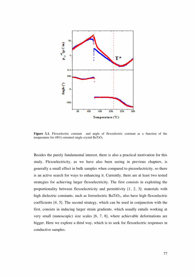
77

Figure 5.1. Flexoelectric constant and angle of flexoelectric constant as a function of the temperature for (001)-oriented single crystal BaTiO3

Besides the purely fundamental interest, there is also a practical motivation for this

study. Flexoelectricity, as we have also been seeing in previous chapters, is

generally a small effect in bulk samples when compared to piezoelectricity, so there

is an active search for ways to enhancing it. Currently, there are at least two tested

strategies for achieving larger flexoelectricity. The first consists in exploiting the

proportionality between flexoelectricity and permittivity [1, 2, 3]: materials with

high dielectric constants, such as ferroelectric BaTiO3, also have high flexoelectric

coefficients [4, 5]. The second strategy, which can be used in conjunction with the

first, consists in inducing larger strain gradients, which usually entails working at

very small (nanoscopic) size scales [6, 7, 8], where achievable deformations are

bigger. Here we explore a third way, which is to seek for flexoelectric responses in

conductive samples.

78

5.2 THE MAXWELL-WAGNER MODEL OF OXYGEN-DEFICIENT BATIO3.

The polarization of an insulating dielectric is limited by how much can its positive

and negative bound charges be separated. However, the effective polarizability of a

device can be enhanced by many orders of magnitude if we also allow free charges

to separate. The physics of this phenomenon has been well understood for more than

a century and is described by the Maxwell-Wagner model [8]. The capacitor

industry has been using the Maxwell-Wagner concept for decades in order to

enhance effective capacitance in devices known as “barrier layer capacitors” [9, 10],

and the Maxwell-Wagner mechanism can also enhance the effective piezoelectricity

of heterogeneous semiconductors [11].

The macroscopic electric properties of materials are characterized by the dielectric

constant ε and conductivity σ. The ratio τ = ε / σ gives a relaxation time for

establishing the steady-state charge distribution after a change in the electric field.

Charge accumulation is allowed at the interface between two materials with

different relaxation times, and this explains the ability of Maxwell-Wagner

capacitors to store more charge than homogeneous dielectrics.

The basic idea behind a barrier layer or Maxwell-Wagner capacitor is depicted in

Figure 5.2: a low-frequency electric field (and by “low frequency” we mean one

slower than the τ time constant of the bulk of the material) is applied to a

heterogeneous material consisting of two thin insulating layers separated by a

semiconducting bulk region, the conducting region responds by allowing its free

charges to move across and accummulate at the interfaces with the insulating region,

and thus the bulk effectively behaves as an intercalated electrode. In this scenario,

only the thin barrier layers at the interface contribute to the total capacitance and,

because capacitance is inversely proportional to thickness, colossal capacitances can

be achieved [9, 10, 12, 13, 14]. Since effective flexoelectricity is proportional to

capacitance (or effective permittivity) this mechanism should also yield ultra-high

effective flexoelectric coefficients.

In order to explore this idea, we have examined the flexoelectricity of single crystal

BaTiO3, oxygen-reduced in order to create oxygen vacancies that act as electron

donors, thus increasing its conductivity [15, 16]. Fully oxidized BaTiO3 (BTO) is

itself an archetypal ferroelectric with a high dielectric permittivity which, as we

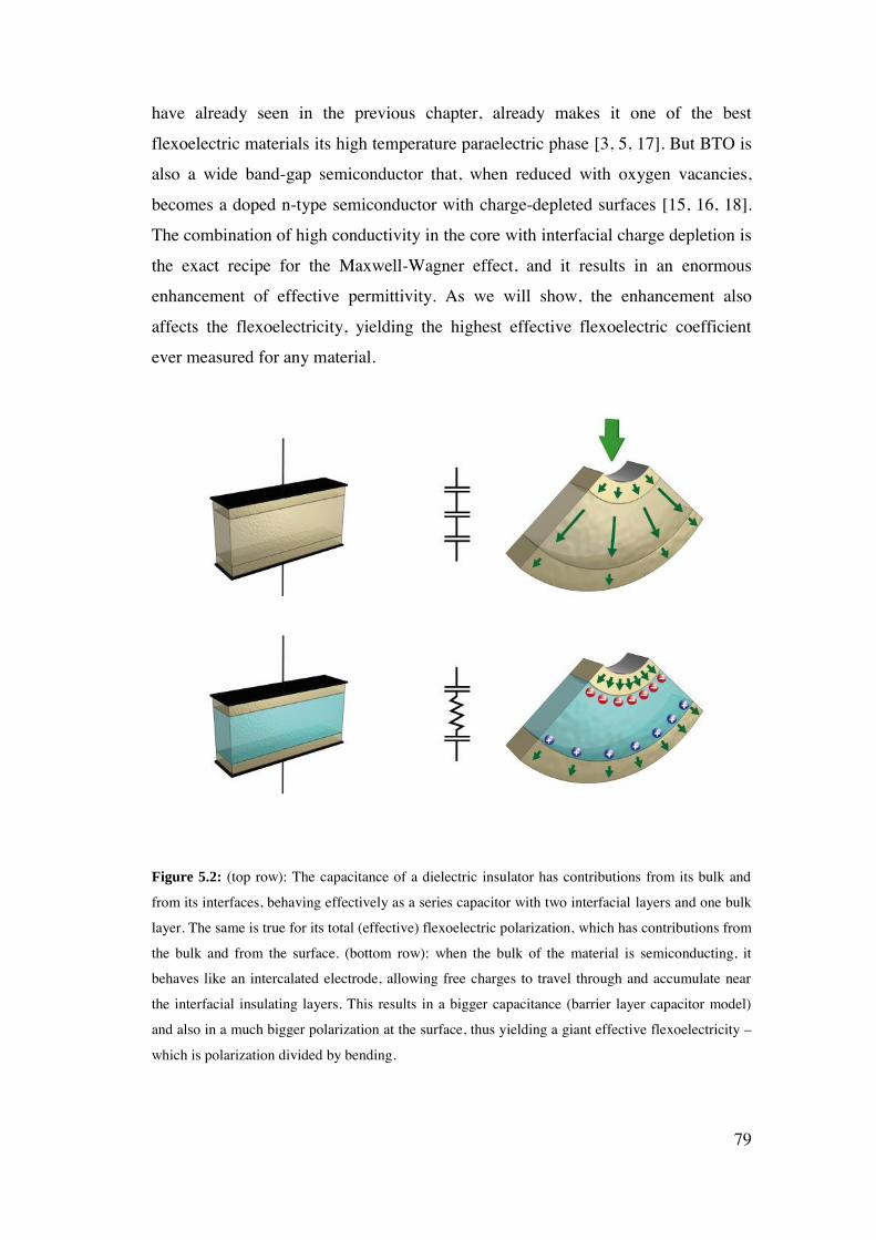
79

have already seen in the previous chapter, already makes it one of the best

flexoelectric materials its high temperature paraelectric phase [3, 5, 17]. But BTO is

also a wide band-gap semiconductor that, when reduced with oxygen vacancies,

becomes a doped n-type semiconductor with charge-depleted surfaces [15, 16, 18].

The combination of high conductivity in the core with interfacial charge depletion is

the exact recipe for the Maxwell-Wagner effect, and it results in an enormous

enhancement of effective permittivity. As we will show, the enhancement also

affects the flexoelectricity, yielding the highest effective flexoelectric coefficient

ever measured for any material.

Figure 5.2: (top row): The capacitance of a dielectric insulator has contributions from its bulk and

from its interfaces, behaving effectively as a series capacitor with two interfacial layers and one bulk

layer. The same is true for its total (effective) flexoelectric polarization, which has contributions from

the bulk and from the surface. (bottom row): when the bulk of the material is semiconducting, it

behaves like an intercalated electrode, allowing free charges to travel through and accumulate near

the interfacial insulating layers. This results in a bigger capacitance (barrier layer capacitor model)

and also in a much bigger polarization at the surface, thus yielding a giant effective flexoelectricity –

which is polarization divided by bending.

80

5.3 DIELECTRIC CHARACTERIZATION OF BATIO3.

The sample used in this work was a single crystal of (001)-oriented BTO,

commercially acquired from SurfaceNet. The sample dimensions were: 1mm wide,

10 mm long and 0.46 mm thick. Measurements made on the as-received sample are

referred to hereon as BTO. Measurements made after reducing the as-received

sample at 900ºC for 2 hours in vacuum atmosphere, are referred to hereon as BTO-δ.

Measurements made after reoxidizing the reduced sample, at 800ºC, for 30 hours in

pure (99.9999%) O2 atmosphere, are referred to hereon as BTO+δ. The method for

measuring the capacitive impedance and flexoelectric coefficient is exactly the same

as in the measurements described in the previous chapters: a dynamic mechanical

analyser connected to a lock-in amplifier was used to measure the bending-induced

displacement current, and an LCR-meter was used to measure the capacitance and

dielectric loss.

50 100 150 200 250 300

Temperature(oC)

1E-3

0.01

0.1

1

10

100

1000

Ta

n(

)

r

1000

10000

100000

1000000

BTO

BTO-

BTO+

Figure 5.3 . Dielectric constant and dielectric loss as a function of temperature for BTO, BTO-δ and

BTO+δ.

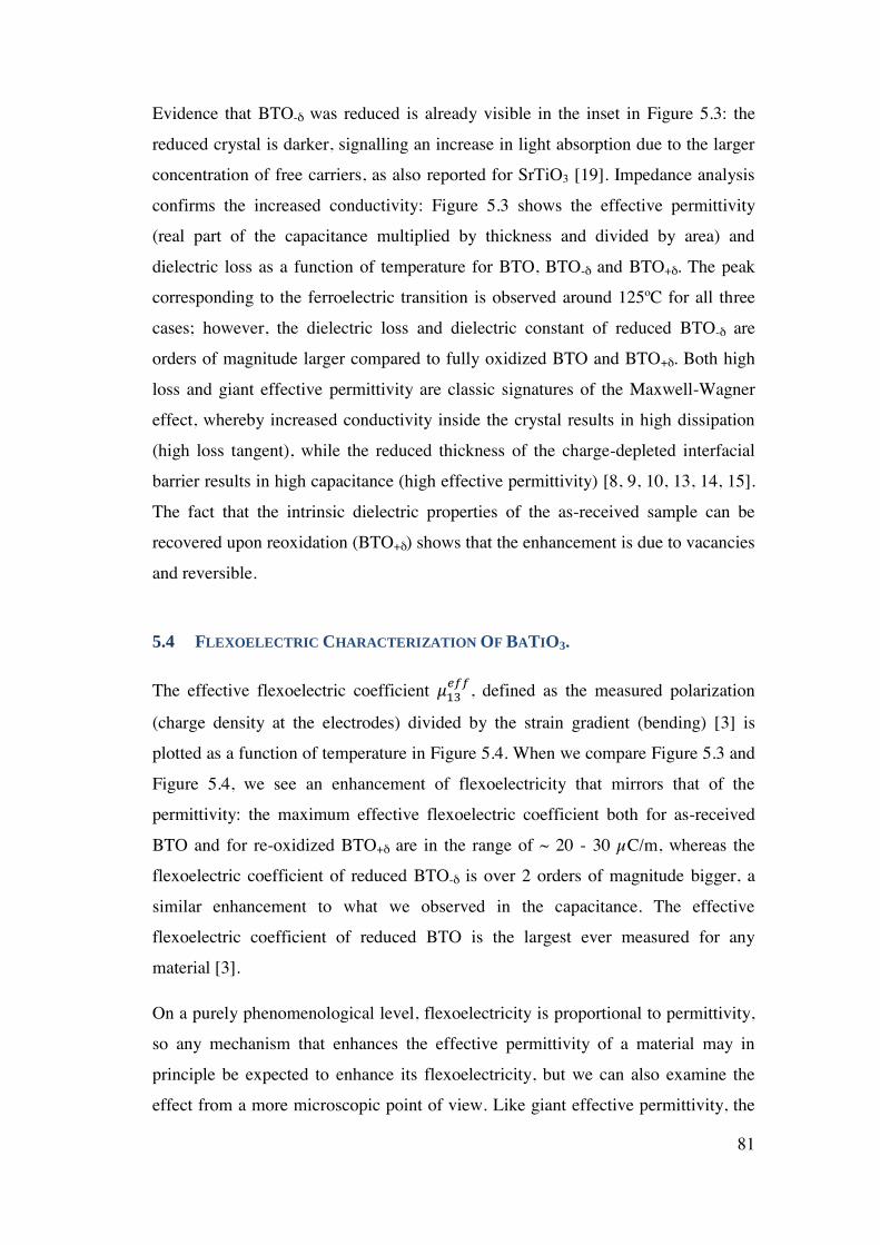
81

Evidence that BTO-δ was reduced is already visible in the inset in Figure 5.3: the

reduced crystal is darker, signalling an increase in light absorption due to the larger

concentration of free carriers, as also reported for SrTiO3 [19]. Impedance analysis

confirms the increased conductivity: Figure 5.3 shows the effective permittivity

(real part of the capacitance multiplied by thickness and divided by area) and

dielectric loss as a function of temperature for BTO, BTO-δ and BTO+δ. The peak

corresponding to the ferroelectric transition is observed around 125ºC for all three

cases; however, the dielectric loss and dielectric constant of reduced BTO-δ are

orders of magnitude larger compared to fully oxidized BTO and BTO+δ. Both high

loss and giant effective permittivity are classic signatures of the Maxwell-Wagner

effect, whereby increased conductivity inside the crystal results in high dissipation

(high loss tangent), while the reduced thickness of the charge-depleted interfacial

barrier results in high capacitance (high effective permittivity) [8, 9, 10, 13, 14, 15].

The fact that the intrinsic dielectric properties of the as-received sample can be

recovered upon reoxidation (BTO+δ) shows that the enhancement is due to vacancies

and reversible.

5.4 FLEXOELECTRIC CHARACTERIZATION OF BATIO3.

The effective flexoelectric coefficient 𝜇13𝑒𝑓𝑓, defined as the measured polarization

(charge density at the electrodes) divided by the strain gradient (bending) [3] is

plotted as a function of temperature in Figure 5.4. When we compare Figure 5.3 and

Figure 5.4, we see an enhancement of flexoelectricity that mirrors that of the

permittivity: the maximum effective flexoelectric coefficient both for as-received

BTO and for re-oxidized BTO+δ are in the range of ~ 20 - 30 µC/m, whereas the

flexoelectric coefficient of reduced BTO-δ is over 2 orders of magnitude bigger, a

similar enhancement to what we observed in the capacitance. The effective

flexoelectric coefficient of reduced BTO is the largest ever measured for any

material [3].

On a purely phenomenological level, flexoelectricity is proportional to permittivity,

so any mechanism that enhances the effective permittivity of a material may in

principle be expected to enhance its flexoelectricity, but we can also examine the

effect from a more microscopic point of view. Like giant effective permittivity, the

82

ultra-large effective flexoelectricity of semiconducting BTO-δ can be explained by

the existence of conductivity with insulating interfacial barrier layers.

Bending always generates at least two electromechanical responses: the bulk

flexoelectric polarization and a surface piezoelectric polarization caused by the

straining of the opposite surface layers (compression on the concave side, tension on

the convex side) [2, 3, 20, 21]. Surface piezoelectricity is itself a necessary

consequence of the fact that interfaces are asymmetric: the material above the

interface (electrode) is different from the material below (BTO). In principle, there

can also be a contribution from surface flexoelectricity, but this is small compared to

the other two for bulk samples [17]: the surface-flexoelectric polarization is of the

same order of magnitude as the bulk flexoelectric polarization, but the thickness

ratio of surface to bulk is small, hence we can neglect it (notice that in surface

piezoelectricity this argument cannot be made, because even though the surface to

bulk ratio is still small, the actual surface polarization grows in direct proportion to

the bulk thickness). The BTO-δ crystal is conducting, and this has two important

consequences: (1) The bulk polarization is screened by free charges [18, 21], so bulk

flexoelectricity cannot contribute to the total polarization, and (2) the free charges

help screen the polar discontinuity between the interfacial layer and the bulk of the

crystal, thus reducing the depolarization field and increasing the piezoelectric

polarization that can be generated by the surface. In effect, the system behaves as if

there were two piezoelectric layers attached to the opposite surfaces of a conducting

slab that acts as an intercalated electrode. Usefully, the surface piezoelectricity is

intrinsic and must exist at all temperatures, irrespective of whether or not the

material is ferroelectric, as we can see from the fact that the large polarization

persists also in the paraelectric phase above the Curie temperature.

In this scenario, the bending-induced charge density is just the product of the surface

piezoelectric coefficient (e) times the surface strain, while the surface strain itself is

the product of the curvature (the strain gradient, G) times the half-thickness of the

crystal, t/2. Thus, the bending-induced surface polarization is

𝑃 = 𝑒𝐺𝑡

2 5.1

83

And therefore, the effective flexoelectric coefficient, defined as the polarization

divided by the strain gradient G, is:

𝜇𝑒𝑓𝑓 = 𝑒𝑡

2 5.2

It is also possible to arrive at equation (5.2) by starting from the general expression

for surface piezoelectricity in a dielectric material [20], 𝜇𝑒𝑓𝑓 = 𝑒𝜆𝑡 𝑏

2𝜆 𝑏+𝑡 𝜆 (where

is the thickness of the surface layer, and b, are respectively the dielectric

constants of the bulk and the surface layers), and setting up the effective permittivity

of the bulk to infinite. Physically, an infinite permittivity is equivalent to a perfect

screening efficiency, so we see that the effect of the conducting layer is indeed to

screen the depolarization field of the piezoelectric interface, thus enhancing the

maximum polarization that can be achieved. Conversely, when the crystal is an

insulating dielectric with a finite permittivity, the contribution from surface

polarization becomes smaller, due to the imperfect screening of the polar

discontinuity. The key message here is therefore that bulk conductivity does not just

allow us to isolate the contribution from surface piezoelectricity (itself a difficult

problem [20, 21, 22, 23], as we discussed in the previous chapter), but to greatly

amplify it to reach values that would be unattainable in insulators.

Usefully, the large bending-induced polarization measured in semiconducting BTO-δ

does NOT require an anomalously large surface piezoelectric coefficient. We can

see this by inverting equation.5.2 in order to calculate the size of the surface

piezoelectric coefficient: 𝑒 =2𝜇𝑒𝑓𝑓

𝑡, where, t is the thickness of our crystal (0.46mm)

and 𝜇13𝑒𝑓𝑓 is the experimentally measured effective flexoelectric coefficient of the

semiconducting crystals (Figure 5.4). Here e is the strain-polarization piezoelectric

coefficient, which can be converted into the more familiar force-charge coefficient

(dij) by multiplying times the elastic compliance [24] (s11 8.5x10-12 Pa-1 for BTO

[25]), hence 𝑑13𝑠𝑢𝑟𝑓

= 𝑠112𝜇13

𝑒𝑓𝑓

𝑡. Substituting the experimentally measured values, we

see that 𝑑13𝑠𝑢𝑟𝑓 ranges from 37 pC/m at Tc down to 0.6 pC/m at 300 oC. These are

modest piezoelectric coefficients by electroceramic standards: the maximum is still

smaller than the bulk piezoelectricity of BaTiO3 (85 pC/m) [16], while the minimum

84

50 100 150 200 250 3000,1

1

10

100

1000Reduced BTO-

Reoxidized BTO+

eff

13(

C/m

)

Temperature (oC)

As-received BTO

Figure 5.4. Effective flexoelectric coefficient as a function of temperature for BTO, BTO-δ and

BTO+δ.

is smaller even than the piezoelectric coefficient of quartz; and yet these fairly

modest piezoelectric coefficients enable effective flexoelectric polarizations orders

of magnitude bigger than would be attainable from the bulk effect alone, as shown

in Figure 5.4.

The conclussions from this investigation into the flexoelectricity of semiconducting

crystals are manifold:

i) Tough in dielectric insulators the contributions from bulk and surface are

inextricably linked [20, 21, 22], by making the bulk conductive it is

experimentally possible to isolate the surface contribution, hitherto an

unsolved scientific problem [23].

ii) Importantly for technological applications, we find that the surface role is

not just comparable to that of the bulk, but it can be much larger, thanks to

screening of the polar discontinuity by the conducting medium: for barium

titanate, the combination of bulk conductivity with modest surface

85

piezoelectricity yields much larger effective flexoelectricity than for the

same crystals in insulating form.

iii) Finally, it is also important to notice that the surface contribution to the

effective flexoelectricity is directly proportional to the thickness (equation

5.2). This cancels the inverse thickness dependence of the strain gradients

[20], and therefore the enhanced bending-induced polarization is

independent of sample size. This means that the enhanced bending-induced

polarization can be important not only at the nanoscale, where conventional

flexoelectricity is already competitive, but also at the macroscale.

iv) The barrier layer mechanism therefore not only breaks beyond the limits of

bulk flexoelectricity in insulators [1, 3, 21] but also, because of its thickness

dependence, it can do so across all device size scales.

5.5 REFERENCES.

1. S. M. Kogan, Sov. Phys. Solid. State 5, 2069 (1964).

2. E. V. Bursian, N.N. Trunov, Sov. Phys. Sol. State 16, 760 (1974).

3. P. Zubko, G. Catalan and A. K. Taganstsev, Ann. Rev. Mater. Res. 43, 387

(2013).

4. E. Bursian and O. I. Zaikovskii, Sov. Phys. Solid State 10, 1121 (1968).


6. G. Catalan, A. Lubk, A. H. G. Vlooswijk, E. Snoeck, C. Magen, A. Janssens, G.

Rispens, G. Rijnders, D. H. A. Blank, and B. Noheda, Nat. Mater. 10, 963 (2011).

7. D. Lee, A. Yoon, S. Y. Jang, J.-G. Yoon, J.-S. Chung, M. Kim, J. F. Scott, and T.

W. Noh, Phys. Rev. Lett. 107, 057602 (2011).

86

8. H. Lu, C.-W. Bark, D. Esque de los Ojos, J. Alcala, C. B. Eom, G. Catalan, A.

Gruverman, Science 336, 59-61 (2012).

9. D. C. Sinclair, T. B. Adams, F. D. Morrison, and A. R. West, Appl. Phys. Lett. 80,

2153 (2002).

10. R. M. Glaister, IEE - Part B: Electronic and Communication Engineering, 109,

423 (1962).

11. D. Damjanovic, M. Demartin Maeder, P. Duran Martin, C. Voisard, and N.

Setter, J. Appl. Phys. 90, 5708 (2001).

12. A. V. Hippel. Dielectrics and Waves, London: Artech House, (1995).

13. D. O’Neill, R. M. Bowman, J. M. Gregg, Appl. Phys. Lett. 77, 1520 (2000).

14. G. Catalan, J. F. Scott. Nature. 448, 7156 (2007).

15. W. Heywang, J. Mater. Science. 6, 1214 (1971).

16. T. Kolodiazhnyi, A. Petric, M. Niewczas, C. Bridges, A. Safa-Sefat, and J. E.

Greedan, Phys. Rev. B. 68, 085205 (2003).

17. L.E. Cross, J. Mater. Sci. 41, 53 (2006).

18. Y. A. Genenko, O. Hirsch and P. Erhart, J. Appl. Phys. 115, 104102 (2014)

19. J. Mannhart, D. G. Schlom, Nature. 430, 620-621 (2004).

20. A.K. Tagantsev, A.S. Yurkov, J. Appl. Phys. 112, 044103 (2012).

21. M. Stengel, Nat. Comm. 4, 2693 (2014).

87


23. J. Narvaez, S. Saremi, J. Hong, M. Stengel, G. Catalan, Phys. Rev. Lett. 115,

037601 (2015)

24. D. Damjanovic, Rep. Prog. Phys. 61, 1267 (1998).

25. D. Berlincourt and H. Jaffe, Phys. Rev. 111, 143 (1958).

88

6 CONCLUSIONS AND FUTURE

DIRECTIONS

89

This thesis is a contribution to research on previously unexplored or unclear

experimental flexoelectricity phenomena on single crystals. We started off by

making the set-up for this type of measurements since is not commercially available.

This setup allowed us to successfully study flexoelectricity on three types of

materials: relaxor ferroelectrics (PMN-PT), ferroelectrics (BTO) and

semiconductors (oxygen-defficient BTO). For each one of the materials, this thesis

work gives an answer to a scientific open question.

In the relaxor-ferroelectric Pb(Mg1/3Nb2/3)O3-PbTiO3 single crystals, we were able

to measure the flexoelectric coefficient as a function of temperature and distinguish

specific phenomena in three ranges of temperature; in the range from 0º to Tc, we

found that the contribution of the polarization was not only flexoelectric but also

piezoelectric; from Tc to T*, we saw a clear evidence of the polar nanoregions

contribution not only from flexoelectric behaviour but also from young’s modulus

curves. The latter statement, confirms the existence of flexoferroelastic contribution

that enhances the polarization in this range of temperature. Finally from T* to

300ºC, we could measure an intrinsic value of flexoelectricity which was according

with the theoretical predictions, with a temperature-independent flexocoupling

coefficient of the order of f =10V. The key message from this investigation is that

the anomalously large flexoelectric enhancement between Tc (or Tm) and T* is due

to mechanically-induced reorientation of ferroelastic polar nanoregions.

In ferroelectric BaTiO3 single crystals, we also saw an enhancement of the

flexoelectric coefficient in the paraelectric phase between Tc and T* attributable to

polar nanoregions as in the case of the relaxor-ferroelectric PMN-PT, but we also

saw an additional and unexpected orientational dependence. By measuring different

orientations of single crystals, we were able to observe a strong anysotropy of the

flexoelectric coefficient in the paraelectric cubic phase that is not consistent with

bulk flexoelectricity in a cubic medium. Using theoretical calculations and

comparing it with experimental data, we conclude that this anisotropy is an indirect

evidence of the surface piezoelectricity contributing to the total effective

flexoelectricity.

Finally, in the n-type semiconductor BaTiO3-δ single crystal, we observed a colossal

value of the effective flexoelectric coefficient (polarization divided by strain

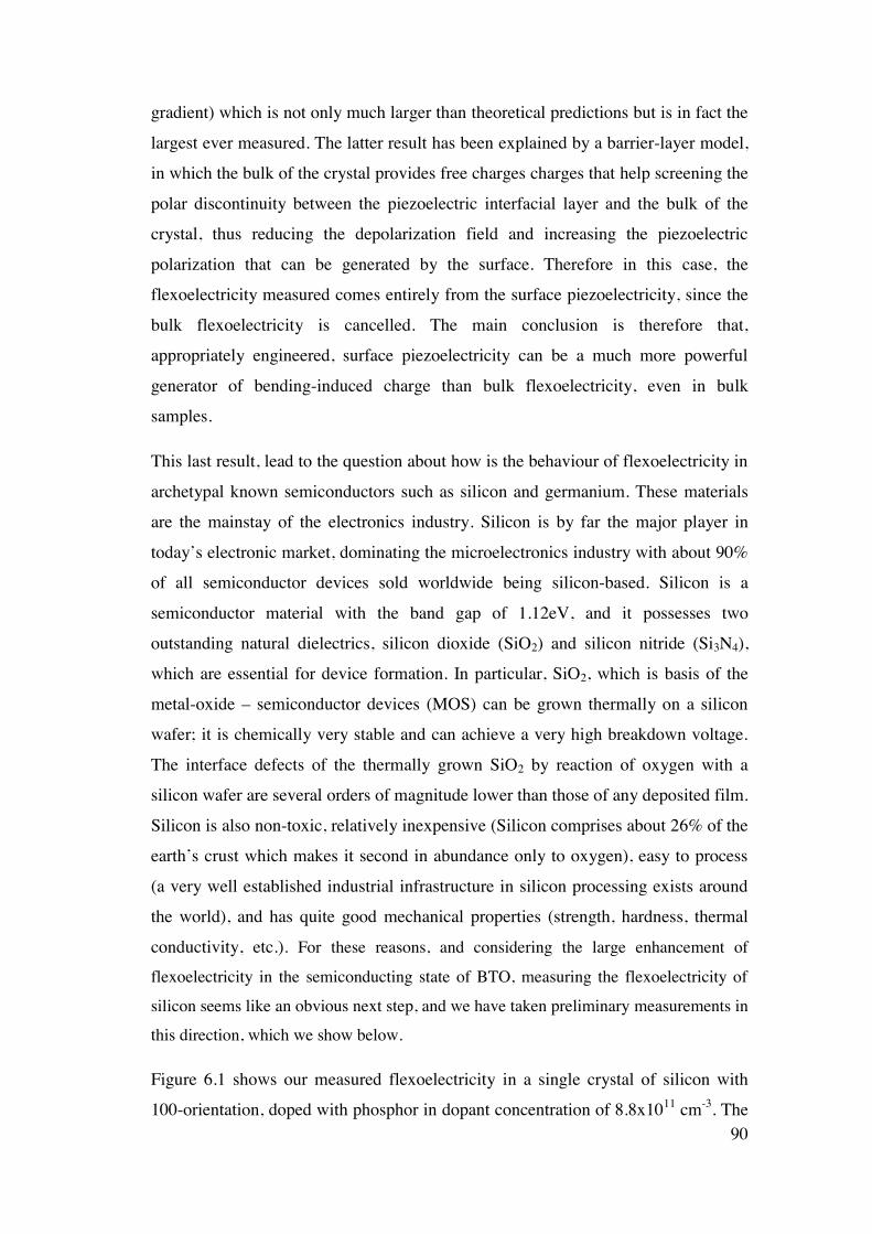
90

gradient) which is not only much larger than theoretical predictions but is in fact the

largest ever measured. The latter result has been explained by a barrier-layer model,

in which the bulk of the crystal provides free charges charges that help screening the

polar discontinuity between the piezoelectric interfacial layer and the bulk of the

crystal, thus reducing the depolarization field and increasing the piezoelectric

polarization that can be generated by the surface. Therefore in this case, the

flexoelectricity measured comes entirely from the surface piezoelectricity, since the

bulk flexoelectricity is cancelled. The main conclusion is therefore that,

appropriately engineered, surface piezoelectricity can be a much more powerful

generator of bending-induced charge than bulk flexoelectricity, even in bulk

samples.

This last result, lead to the question about how is the behaviour of flexoelectricity in

archetypal known semiconductors such as silicon and germanium. These materials

are the mainstay of the electronics industry. Silicon is by far the major player in

today’s electronic market, dominating the microelectronics industry with about 90%

of all semiconductor devices sold worldwide being silicon-based. Silicon is a

semiconductor material with the band gap of 1.12eV, and it possesses two

outstanding natural dielectrics, silicon dioxide (SiO2) and silicon nitride (Si3N4),

which are essential for device formation. In particular, SiO2, which is basis of the

metal-oxide – semiconductor devices (MOS) can be grown thermally on a silicon

wafer; it is chemically very stable and can achieve a very high breakdown voltage.

The interface defects of the thermally grown SiO2 by reaction of oxygen with a

silicon wafer are several orders of magnitude lower than those of any deposited film.

Silicon is also non-toxic, relatively inexpensive (Silicon comprises about 26% of the

earth’s crust which makes it second in abundance only to oxygen), easy to process

(a very well established industrial infrastructure in silicon processing exists around

the world), and has quite good mechanical properties (strength, hardness, thermal

conductivity, etc.). For these reasons, and considering the large enhancement of

flexoelectricity in the semiconducting state of BTO, measuring the flexoelectricity of

silicon seems like an obvious next step, and we have taken preliminary measurements in

this direction, which we show below.

Figure 6.1 shows our measured flexoelectricity in a single crystal of silicon with

100-orientation, doped with phosphor in dopant concentration of 8.8x1011 cm-3. The

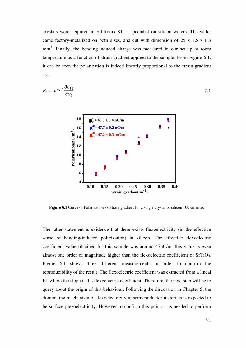
91

crystals were acquired in Sil’tronix-ST, a specialist on silicon wafers. The wafer

came factory-metalized on both sizes, and cut with dimension of 25 x 1.5 x 0.3

mm3. Finally, the bending-induced charge was measured in our set-up at room

temperature as a function of strain gradient applied to the sample. From Figure 6.1,

it can be seen the polarization is indeed linearly proportional to the strain gradient

as:

𝑃3 = 𝜇𝑒𝑓𝑓𝜕𝜖11

𝜕𝑥3 7.1

0.10 0.15 0.20 0.25 0.30 0.35 0.404

6

8

10

12

14

16

18

eff

13= 47.2 ± 0.3 nC/m

eff

13= 47.7 ± 0.2 nC/m

eff

13= 46.3 ± 0.4 nC/m

Po

lariz

ati

on

(nC

/m2

)

Strain gradient(m-1)

Figure 6.1 Curve of Polarization vs Strain gradient for a single crystal of silicon 100-oriented

The latter statement is evidence that there exists flexoelectricity (in the effective

sense of bending-induced polarization) in silicon. The effective flexoelectric

coefficient value obtained for this sample was around 47nC/m; this value is even

almost one order of magnitude higher than the flexoelectric coefficient of SrTiO3.

Figure 6.1 shows three different measurements in order to confirm the

reproducibility of the result. The flexoelectric coefficient was extracted from a lineal

fit, where the slope is the flexoelectric coefficient. Therefore, the next step will be to

query about the origin of this behaviour. Following the discussion in Chapter 5, the

dominating mechanism of flexoelectricity in semiconductor materials is expected to

be surface piezoelectricity. However to confirm this point; it is needed to perform

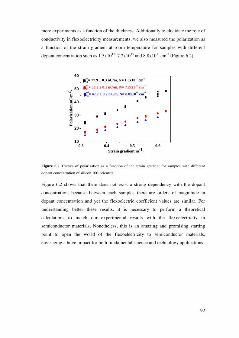
92

more experiments as a function of the thickness. Additionally to elucidate the role of

conductivity in flexoelectricity measurements, we also measured the polarization as

a function of the strain gradient at room temperature for samples with different

dopant concentration such as 1.5x1017, 7.2x1015 and 8.8x1011 cm-3 (Figure 6.2).

0.3 0.4 0.5 0.610

20

30

40

50

60

eff

13= 53.2 ± 0.1 nC/m, N= 7.2x10

15 cm

-3

eff

13= 77.9 ± 0.3 nC/m, N= 1.5x10

17 cm

-3

Po

lariz

ati

on

(nC

/m2

)

Strain gradient(m-1)

eff

13= 47.7 ± 0.2 nC/m, N= 8.8x10

11 cm

-3

Figure 6.2. Curves of polarization as a function of the strain gradient for samples with different

dopant concentration of silicon 100-oriented

Figure 6.2 shows that there does not exist a strong dependency with the dopant

concentration, because between each samples there are orders of magnitude in

dopant concentration and yet the flexoelectric coefficient values are similar. For

understanding better these results, it is necessary to perform a theoretical

calculations to match our experimental results with the flexoelectricity in

semiconductor materials. Nonetheless, this is an amazing and promising starting

point to open the world of the flexoelectricity to semiconductor materials,

envisaging a huge impact for both fundamental science and technology applications.

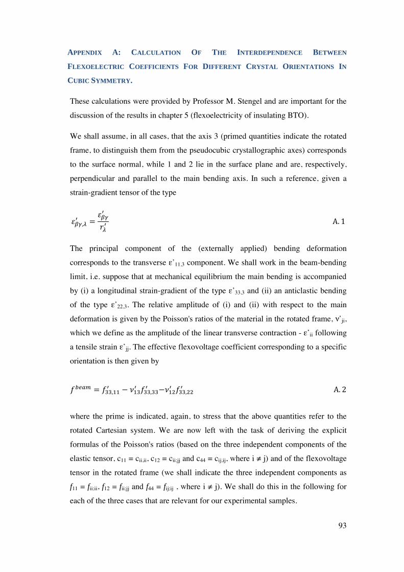
93

APPENDIX A: CALCULATION OF THE INTERDEPENDENCE BETWEEN

FLEXOELECTRIC COEFFICIENTS FOR DIFFERENT CRYSTAL ORIENTATIONS IN

CUBIC SYMMETRY.

These calculations were provided by Professor M. Stengel and are important for the

discussion of the results in chapter 5 (flexoelectricity of insulating BTO).

We shall assume, in all cases, that the axis 3 (primed quantities indicate the rotated

frame, to distinguish them from the pseudocubic crystallographic axes) corresponds

to the surface normal, while 1 and 2 lie in the surface plane and are, respectively,

perpendicular and parallel to the main bending axis. In such a reference, given a

strain-gradient tensor of the type

휀𝛽𝛾,𝜆′ =

휀𝛽𝛾′

𝑟𝜆′ A. 1

The principal component of the (externally applied) bending deformation

corresponds to the transverse ε’11,3 component. We shall work in the beam-bending

limit, i.e. suppose that at mechanical equilibrium the main bending is accompanied

by (i) a longitudinal strain-gradient of the type ε’33,3 and (ii) an anticlastic bending

of the type ε’22,3. The relative amplitude of (i) and (ii) with respect to the main

deformation is given by the Poisson's ratios of the material in the rotated frame, ν’ji,

which we define as the amplitude of the linear transverse contraction - ε’ii following

a tensile strain ε’jj. The effective flexovoltage coefficient corresponding to a specific

orientation is then given by

𝑓𝑏𝑒𝑎𝑚 = 𝑓33,11′ − 𝜈13

′ 𝑓33,33′ −𝜈12

′ 𝑓33,22′ A. 2

where the prime is indicated, again, to stress that the above quantities refer to the

rotated Cartesian system. We are now left with the task of deriving the explicit

formulas of the Poisson's ratios (based on the three independent components of the

elastic tensor, c11 = cii,ii, c12 = cii;jj and c44 = cij,ij, where i ≠ j) and of the flexovoltage

tensor in the rotated frame (we shall indicate the three independent components as

f11 = fii;ii, f12 = fii;jj and f44 = fij;ij , where i ≠ j). We shall do this in the following for

each of the three cases that are relevant for our experimental samples.

94

(100) ORIENTATION

This is the simplest case - no rotation of the crystal axes is needed here. We have,

for the Poisson's ratios

𝜈 = 𝜈13 = 𝜈12 =𝑐12

𝑐11 + 𝑐12 A. 3

Then, we can immediately write

𝑓100𝑏𝑒𝑎𝑚 = (1 − 𝜈)𝑓12 − 𝜈𝑓11 A. 4

This coincides with the result of Zubko et al [1].

(110) ORIENTATION

First, we define the rotated reference frame,

x1′ =

1

√2(1, 1, 0) A. 5

x2′ = (0, 0, 1) A. 6

x3′ =

1

√2(1, 1, 0) A. 7

where, as above, 3' is the longitudinal (normal to the surface) direction, 1' is the

transverse direction, and 2' is the main bending axis. (Recall that, as we are working

in the beam limit, there is an anticlastic bending about the 1' axis).

The Poisson's ratios are easiest to express in term of the compliances, ν’ji = -sij/sjj. In

our case, this yields

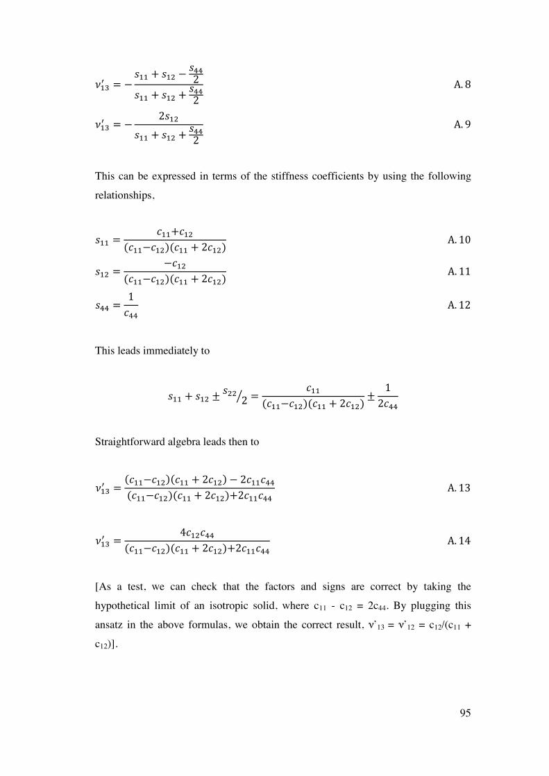
95

𝜈13′ = −

𝑠11 + 𝑠12 −𝑠44

2

𝑠11 + 𝑠12 +𝑠44

2

A. 8

𝜈13′ = −

2𝑠12

𝑠11 + 𝑠12 +𝑠44

2

A. 9

This can be expressed in terms of the stiffness coefficients by using the following

relationships,

𝑠11 =𝑐11+𝑐12

(𝑐11−𝑐12)(𝑐11 + 2𝑐12) A. 10

𝑠12 =−𝑐12

(𝑐11−𝑐12)(𝑐11 + 2𝑐12) A. 11

𝑠44 =1

𝑐44 A. 12

This leads immediately to

𝑠11 + 𝑠12 ±𝑠22

2⁄ =𝑐11

(𝑐11−𝑐12)(𝑐11 + 2𝑐12)±

1

2𝑐44

Straightforward algebra leads then to

𝜈13′ =

(𝑐11−𝑐12)(𝑐11 + 2𝑐12) − 2𝑐11𝑐44

(𝑐11−𝑐12)(𝑐11 + 2𝑐12)+2𝑐11𝑐44 A. 13

𝜈13′ =

4𝑐12𝑐44

(𝑐11−𝑐12)(𝑐11 + 2𝑐12)+2𝑐11𝑐44 A. 14

[As a test, we can check that the factors and signs are correct by taking the

hypothetical limit of an isotropic solid, where c11 - c12 = 2c44. By plugging this

ansatz in the above formulas, we obtain the correct result, ν’13 = ν’12 = c12/(c11 +

c12)].

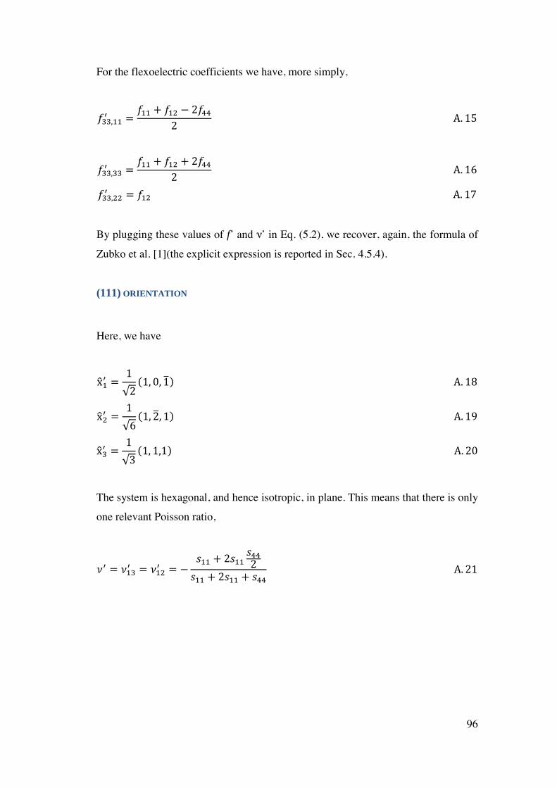
96

For the flexoelectric coefficients we have, more simply,

𝑓33,11′ =

𝑓11 + 𝑓12 − 2𝑓44

2 A. 15

𝑓33,33′ =

𝑓11 + 𝑓12 + 2𝑓44

2 A. 16

𝑓33,22′ = 𝑓12 A. 17

By plugging these values of f’ and ν’ in Eq. (5.2), we recover, again, the formula of

Zubko et al. [1](the explicit expression is reported in Sec. 4.5.4).

(111) ORIENTATION

Here, we have

x1′ =

1

√2(1, 0, 1) A. 18

x2′ =

1

√6(1, 2, 1) A. 19

x3′ =

1

√3(1, 1,1) A. 20

The system is hexagonal, and hence isotropic, in plane. This means that there is only

one relevant Poisson ratio,

𝜈′ = 𝜈13′ = 𝜈12

′ = −𝑠11 + 2𝑠11

𝑠44

2𝑠11 + 2𝑠11 + 𝑠44

A. 21

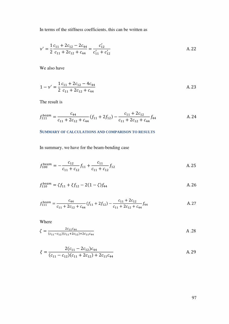
97

In terms of the stiffness coefficients, this can be written as

𝜈′ =1

2

𝑐11 + 2𝑐12 − 2𝑐44

𝑐11 + 2𝑐12 + 𝑐44=

𝑐12′

𝑐11′ + 𝑐12

′ A. 22

We also have

1 − 𝜈′ =1

2

𝑐11 + 2𝑐12 − 4𝑐44

𝑐11 + 2𝑐12 + 𝑐44 A. 23

The result is

𝑓111𝑏𝑒𝑎𝑚 =

𝑐44

𝑐11 + 2𝑐12 + 𝑐44

(𝑓11 + 2𝑓12) −𝑐11 + 2𝑐12

𝑐11 + 2𝑐12 + 𝑐44𝑓44 A. 24

SUMMARY OF CALCULATIONS AND COMPARISON TO RESULTS

In summary, we have for the beam-bending case

𝑓100𝑏𝑒𝑎𝑚 = −

𝑐12

𝑐11 + 𝑐12𝑓11 +

𝑐11

𝑐11 + 𝑐12𝑓12 A. 25

𝑓110𝑏𝑒𝑎𝑚 = 휁𝑓11 + 𝜉𝑓12 − 2(1 − 휁)𝑓44 A. 26

𝑓111𝑏𝑒𝑎𝑚 =

𝑐44

𝑐11 + 2𝑐12 + 𝑐44

(𝑓11 + 2𝑓12) −𝑐11 + 2𝑐12

𝑐11 + 2𝑐12 + 𝑐44𝑓44 A. 27

Where

휁 =2𝑐11𝑐44

(𝑐11−𝑐12)(𝑐11+2𝑐12)+2𝑐11𝑐44 A .28

𝜉 =2(𝑐11 − 2𝑐12)𝑐44

(𝑐11 − 𝑐12)(𝑐11 + 2𝑐12) + 2𝑐11𝑐44 A. 29

98

So, let's check the linear dependence above. We need to multiply f110 by

(𝑐11 − 𝑐12)(𝑐11 + 2𝑐12) + 2𝑐11𝑐44

2(𝑐11 − 𝑐12)

and then subtract f111(c11 + 2c12 + c44). We have, for the coefficient of f11,

𝑐11𝑐44

𝑐11 − 𝑐12− 𝑐44 =

𝑐12𝑐44

𝑐11 − 𝑐12

Regarding f12, we have

(𝑐11 − 2𝑐12)𝑐44

𝑐11 − 𝑐12− 2𝑐44 =

−𝑐11𝑐44

𝑐11 − 𝑐12

The result is

−(𝐶11 − 𝐶12)(𝐶11 + 2𝐶12) + 2𝐶11𝐶44

2𝐶44(𝐶11 − 𝐶12)𝑓110

𝑏𝑒𝑎𝑚

+(𝐶11 + 2𝐶12 + 4𝐶44)(𝐶11 − 𝐶12)

𝐶44(𝐶11 + 𝐶12)𝑓111

𝑏𝑒𝑎𝑚 = 𝑓100𝑏𝑒𝑎𝑚 A. 30

One can check the consistency of the above in the isotropic case, where we have

3𝑓111𝑏𝑒𝑎𝑚 − 2𝑓110

𝑏𝑒𝑎𝑚 = 𝑓100𝑏𝑒𝑎𝑚. To apply this to BaTiO3 we use the following

experimental values for the elastic (stiffness) contants: c11 = 173 GPa, c12 = 82 GPa,

c44 = = = 108 GPa. We obtain

1.47𝑓111𝑏𝑒𝑎𝑚 − 1.24𝑓110

𝑏𝑒𝑎𝑚 = 𝑓100𝑏𝑒𝑎𝑚 A. 31

REFERENCES


Lett. 99, 167601 (2007).

ADVERTIMENT. Lʼaccés als continguts dʼaquesta tesi queda ... · A diferencia del efecto...

Documents

Transcript of ADVERTIMENT. Lʼaccés als continguts dʼaquesta tesi queda ... · A diferencia del efecto...