HIGH VELOCITY OUTFLOWS IN QUASARS

By

PAOLA RODRIGUEZ

A DISSERTATION PRESENTED TO THE GRADUATE SCHOOLOF THE UNIVERSITY OF FLORIDA IN PARTIAL FULFILLMENT

OF THE REQUIREMENTS FOR THE DEGREE OFDOCTOR OF PHILOSOPHY

UNIVERSITY OF FLORIDA

2009

1

c© 2009 Paola Rodrıguez

2

To my mother, my family and my friends, because without their support I am nothing

3

ACKNOWLEDGMENTS

I was told long time ago that “es de buen nacido ser agradecido”. Como mi madre me

educo muy bien, no puedo evitar intentar incluir a todos aquellos que me han ayudado y

que son parte importante de esta tesis. I am happy to say that I could not have done this

without the help of many great people that I have had the pleasure and luck of meeting

during these last six years. I hope my memory does not fail me here. To start, I would

like to thank Ramon Garcıa Lopez, because without his encouragement and help I would

have not applied to the UF Alumni Fellowship and become the first Spanish graduate

student in the UF-IAC exchange program. Once I arrived, Rafael Guzman and who later

became my adviser, Fred Hamann, were an incredible help to make the transition easier.

For all her help, for always being there, and for being a super mom to all the international

kids, I would like to thank Debra Anderson and everybody I met at the UF International

Center. All of you are amazing! Those first moments in Gainesville were not easy . . .

and as the song says, I would not have done it without (more than) a little help from

my friends, and especially I would like to thank Ana, Eric, Ily, Katherine, Bruno, Pimol,

Alister and Balsa for making it much more fun. Margaret: thank you so much for your

friendship, for being always “my rock”, for all the drinks and the laughs. Those parties

were always crazy and Sundays would not have been so bright without brunch! I would

like to thank Ashley for being herself all the time, for the laughs, the help and the jacket!

I am going to randomly ask people in my future office to start screaming when I miss

you, Sun. Thanks go to her and Audra for all those night outs and talks. I would like to

thank my partners in crime, Leah, Dan C. and Dan B. for being an amazing group (and

a great release when I needed to complain about my adviser). I would like to thank my

roommate, one of my best friends, and my partner in ball games at 2am in the third floor

corridor, Curtis, for always being there and for his never ending kindness. I would like to

thank Suvrath and Maren for all the advice and Julian for being such a good person (and

not forcing me to try marmite ever again!). A mi hermanito Miguel solo le puedo decir

4

“feo, gracias por todo!! que la distancia solo nos mantenga mas cerca”. A toda la “Spanish

troupe” (Nestor, Jorge, Izaskun y Enrique) por esas comidas de 5 horas y por las risas

(al final, Izaskun nunca aparco el coche delante de mi casita del downtown . . .). Dave

and Knicole arrived at the end to make my last year hilarious and much more difficult

to leave . . . Keep on rocking! I also have an American brother, Justin: thank you so

much for being a companion until the early hours of the morning and for all those laughs

(although I still want to kill you for not telling me Amy was pregnant until her 6th month

of pregnancy . . .). Thanks go to Dimitri for the late night talks, for the cookies and for

the all the reading (you are amazing). To Elizabeth, my wonderful girlfriend, for being the

least complicated relationship I have ever been into. I wish you all had arrived earlier! To

Nancy, for accepting the mess I had made in my office and to her and PC for being my

officemates when nobody else was there. To all my other officemates during these years

for accepting me whenever I was stressed and for laughing while working. Thanks go to

Craig (Go Gators!) for being such an IDL machine and for all the beer . . . I would also

like to thank Anthony Gonzalez for letting me annoy him every time I wanted, for all

his advice and for the use of his laptop when mine crashed two months before I finished

my dissertation. I especially remembered what he said when I got offered a post-doctoral

position and it was official that I was leaving “Oh wow, it seems like yesterday when you

arrived and complained about everything . . .” I would like to thank those who became

my other American family, Ben and Leah, and very especially Joanne, for their friendship

and encouragement. Also, my thanks go to all the wonderful professors that have taught

me so much about this wonderful world of physics and astronomy, and to Catherine

for keeping me updated with what I had to do, especially when I had lost control of

everything . . . And finally to the friends I found at the very end of my experience in

Gainesville: all the latin crowd, and especially Cynna and Leila, let’s toast for the shared

moments we will have in the future!

5

Sin embargo, mi aventura empezo mucho antes. Me gustarıa dar las gracias a mis

profesores Nestor Rodrıguez e Irene Puerto por ser una inspiracion para mi, por despertar

mi espıritu crıtico y mi amor por la fısica. Tambien me gustarıa dar las gracias a mis

amigos de casa y a los que ya estan repartidos por el mundo. A mi mejor amiga, Noa,

por todas esas llamadas y mailes cuando la desesperacion de estar tan lejos se hacıa

insoportable y por mantener el cordon unido para que pareciera que nunca me habıa ido

del todo, gracias de todo corazon. A ella y a Carlos, Rocıo, Marta, Gema, Bea y Ana por

las risas y por compartir los cambios en nuestras vidas aunque estuvieramos lejos, por las

comidas paralelas, por esas tarjetas manufacturadas estupendas, y por esas celebraciones

conjuntas que nos echamos, sois los mejores amigos que podrıa tener. A Eduardo, por

convertirse en una de las personas mas importantes en mi vida y nunca dejar de serlo.

Aunque seguimos sin encontrarnos a este o al otro lado del charco, siempre espero verte

pronto! La antesala de esta tesis, mis dos anos en Canarias, ya me presento un monton

de gente estupenda que afortunadamente continua en mi vida. Raquel, gracias por ser la

mejor companera de aventuras en la distancia. No se que habrıa hecho sin nuestras charlas

diarias. Gracias a Susi, Vane, Merche, Ana, David, Panete, y en especial a Carlos, por

todas esas risas ciberneticas que han hecho, y hacen, que los dıas de trabajo sean mucho

mas amenos (y sigo pensando sin embargo que Notting Hill es una basura . . .!!) Gracias a

todos ellos he aprendido que la distancia es, en verdad, relativa.

I would like to thank my committee, Stephen Eikenberry, James Fry, Vicki Sarajedini

and Jonathan Tan, and especially Michael Crenshaw, for their endless patience, their

multiple comments and questions. Without any doubt, the maximum contributor to make

this dissertation possible is my adviser, Fred Hamann. Fred, I would like to thank you

for so many things I would need another whole acknowledgements section just for it. You

have taught me everything I know about quasar outflows, and have been a mentor and

a friend. You are also one of the people I respect more in this field. I also would like to

thank you for all the good (and not so good) shared moments, because life happens while

6

you are working on and writing the dissertation . . . Thank you so much for everything,

from the beginning, when my English was so bad we needed to play pictionary to be

able to have a meeting, to the last moments, when we would help each other in the panic

crises. Also, I would like to thank you (really!) for your many, many, (many!) comments.

I am sure I will know when you are the referee of one of my papers . . . And just so you

know, leaving your office for the very last time as one of your graduate students was a very

emotional moment.

Fortunately, people in my field are very cool, choose very cool places to have

workshops, and I have had the pleasure of meeting many of them. I would like to thank

Michael Crenshaw, George Chartas, Doron Chelouche, Michael Eracleous, Paul Green,

Jason X. Prochaska, and Daniel Proga, Joe Shields for many helpful discussions and

becoming collaborators. I would also like to thank the support of the KPNO and MDM

observatories scientists and staff. In particular, I would like to send our thanks to John

Thorsten, Steven Magee, and Robert Barr for solving the mystery of the “rare gas”

spectral lines at the MDM observatory, and Doug Williams, Hal Haldebel, Jin Hutchinson,

Karen Butler, Dianne Harmer, Gene McDougall, and Kristin Reetz especially, for their

help during telescope “crises” at the 2.1 m. And many thanks go to my future boss, Jane

Charlton, for waiting for me all these last months that took to finish my dissertation.

De vuelta en casa, gracias a toda mi familia, por aun sin entender que me pasara el

tiempo “mirando estrellitas” nunca dejaron de darme su amor y apoyo desde la distancia,

y en especial a mis “papis”: Arturo, Anıbal y Luis, por ejercer de figura paterna, cada

uno a su estilo y a su forma. Gracias por esas multitudinarias comidas organizadas en

el ultimo momento, por esas charlas acerca de la vida, de la ciencia y lo que la carrera

significaba y por los constantes chequeos para ver que seguıa bien y con los pies en el

suelo. A mi abuela Elisa que se fue mientras empezaba esta tesis pero sigue presente, y a

mi abuela Amelia, por que podamos compartir muchos mas momentos.

7

Y gracias a Alejandro (Ale! Ale! Ale!), porque despues de haber cruzado el charco

tantas veces hay momentos que una ya no sabe de donde es, y por fin encontre “casa”

cuando te conocı. Gracias por tener siempre la mirada perfecta y la palabra precisa. Soy

la mas afortunada (the luckiest) por recibir ese amor tan bonito que llego cuando menos

me lo esperaba. Gracias por esa felicidad contagiosa que me das, que provoca la carcajada

diaria, y por bancarme cuando la pierdo. Te amo guachi!!

Y por supuesto, a mi mami, porque sin ti no estarıa aquı. Gracias por poner mi

educacion por delante de todo y por tu guıa constante, y especialmente por tu apoyo

incondicional cuando me iba cada vez mas lejos. Estamos tan lejos y tan cerca a la vez, no

crees? Gracias por ser la mejor mami del mundo. Con cuatro anos te decıa que te querıa

de aquı a la luna (ida y vuelta, no te vayas a creer . . .) Despues aprendı que te querıa de

aquı a Pluton (ya no es un planeta, vale, pero la distancia es la misma.) Con el tiempo

he aprendido no solo que el universo era mucho mas grande y que se expande, sino que el

amor que se tiene por una madre es mucho mas grande tambien y crece en la distancia y

hoy puedo decir: “Mami, te quiero de aquı a los quasares!!!”

8

TABLE OF CONTENTS

page

ACKNOWLEDGMENTS . . . . . . . . . . . . . . . . . . . . . . . . . . . . . . . . . 4

LIST OF TABLES . . . . . . . . . . . . . . . . . . . . . . . . . . . . . . . . . . . . . 11

LIST OF FIGURES . . . . . . . . . . . . . . . . . . . . . . . . . . . . . . . . . . . . 12

ABSTRACT . . . . . . . . . . . . . . . . . . . . . . . . . . . . . . . . . . . . . . . . 14

CHAPTER

1 INTRODUCTION . . . . . . . . . . . . . . . . . . . . . . . . . . . . . . . . . . 16

1.1 Quasars . . . . . . . . . . . . . . . . . . . . . . . . . . . . . . . . . . . . . 161.2 Quasar Outflows . . . . . . . . . . . . . . . . . . . . . . . . . . . . . . . . 181.3 Variability of Outflows . . . . . . . . . . . . . . . . . . . . . . . . . . . . . 221.4 Goals . . . . . . . . . . . . . . . . . . . . . . . . . . . . . . . . . . . . . . . 23

2 HIGH VELOCITY OUTFLOW IN QUASAR PG0935+417 . . . . . . . . . . . 25

2.1 Introduction . . . . . . . . . . . . . . . . . . . . . . . . . . . . . . . . . . . 252.2 Data . . . . . . . . . . . . . . . . . . . . . . . . . . . . . . . . . . . . . . . 262.3 Analysis . . . . . . . . . . . . . . . . . . . . . . . . . . . . . . . . . . . . . 28

2.3.1 Line Identification . . . . . . . . . . . . . . . . . . . . . . . . . . . . 282.3.2 Continuum Normalization . . . . . . . . . . . . . . . . . . . . . . . 302.3.3 Line Measurements and Physical Quantities . . . . . . . . . . . . . 34

2.4 Discussion . . . . . . . . . . . . . . . . . . . . . . . . . . . . . . . . . . . . 392.4.1 Ionization and Total Column Density of the Outflow . . . . . . . . . 392.4.2 Nature of the Absorber, Variability and Kinematics . . . . . . . . . 412.4.3 Origin of the Outflow, Timescales and Causes for Variability . . . . 43

2.5 Conclusion . . . . . . . . . . . . . . . . . . . . . . . . . . . . . . . . . . . . 46

3 AN INVENTORY OF C IV MINI-BALS AND OUTFLOW LINES IN SDSSQUASARS . . . . . . . . . . . . . . . . . . . . . . . . . . . . . . . . . . . . . . 48

3.1 Introduction . . . . . . . . . . . . . . . . . . . . . . . . . . . . . . . . . . . 483.2 Quasar Sample . . . . . . . . . . . . . . . . . . . . . . . . . . . . . . . . . 493.3 Identification and Measurements of C iv Absorption Lines . . . . . . . . . 503.4 Mini-BALs . . . . . . . . . . . . . . . . . . . . . . . . . . . . . . . . . . . . 593.5 Statistics . . . . . . . . . . . . . . . . . . . . . . . . . . . . . . . . . . . . . 64

3.5.1 Statistics of Mini-BALs . . . . . . . . . . . . . . . . . . . . . . . . . 663.5.2 Relation between Mini-BALs and BALs . . . . . . . . . . . . . . . . 713.5.3 Relation between Mini-BALs and AALs . . . . . . . . . . . . . . . . 743.5.4 Relation between C iv Mini-BALs and Mg ii Absorption . . . . . . 773.5.5 Relation between C iv Mini-BALs and Radio Properties . . . . . . . 79

9

3.6 Discussion . . . . . . . . . . . . . . . . . . . . . . . . . . . . . . . . . . . . 823.7 Summary and Conclusions . . . . . . . . . . . . . . . . . . . . . . . . . . . 91

4 VARIABILITY IN QUASAR OUTFLOWS . . . . . . . . . . . . . . . . . . . . 93

4.1 Introduction . . . . . . . . . . . . . . . . . . . . . . . . . . . . . . . . . . . 934.2 Sample Selection and Observations . . . . . . . . . . . . . . . . . . . . . . 934.3 Data Reduction and Measurements . . . . . . . . . . . . . . . . . . . . . . 944.4 Analysis . . . . . . . . . . . . . . . . . . . . . . . . . . . . . . . . . . . . . 114

4.4.1 Characterizing the Variability . . . . . . . . . . . . . . . . . . . . . 1144.4.2 Variability Fractions and Trends . . . . . . . . . . . . . . . . . . . . 1154.4.3 Comparisons to Previous Work on BALs . . . . . . . . . . . . . . . 123

4.5 Discussion . . . . . . . . . . . . . . . . . . . . . . . . . . . . . . . . . . . . 1244.5.1 Summary of Main Results . . . . . . . . . . . . . . . . . . . . . . . 1244.5.2 Physical Properties of the Absorbers and Variability Causes . . . . . 124

4.5.2.1 Change of the ionization state . . . . . . . . . . . . . . . . 1254.5.2.2 Motion of the absorber . . . . . . . . . . . . . . . . . . . . 127

5 SUMMARY AND CONCLUSIONS . . . . . . . . . . . . . . . . . . . . . . . . . 129

APPENDIX: ADDITIONAL OBSERVATIONS . . . . . . . . . . . . . . . . . . . . . 131

A.1 J083104+532500 . . . . . . . . . . . . . . . . . . . . . . . . . . . . . . . . 131A.2 J092849+504930 . . . . . . . . . . . . . . . . . . . . . . . . . . . . . . . . 131A.3 J093857+412821 . . . . . . . . . . . . . . . . . . . . . . . . . . . . . . . . 132A.4 J102907+651024 . . . . . . . . . . . . . . . . . . . . . . . . . . . . . . . . 132A.5 J103859+484049 . . . . . . . . . . . . . . . . . . . . . . . . . . . . . . . . 132A.6 J144105+045454 . . . . . . . . . . . . . . . . . . . . . . . . . . . . . . . . 133A.7 J163651+313147 . . . . . . . . . . . . . . . . . . . . . . . . . . . . . . . . 134

REFERENCES . . . . . . . . . . . . . . . . . . . . . . . . . . . . . . . . . . . . . . . 135

BIOGRAPHICAL SKETCH . . . . . . . . . . . . . . . . . . . . . . . . . . . . . . . . 141

10

LIST OF TABLES

Table page

2-1 Observation logs . . . . . . . . . . . . . . . . . . . . . . . . . . . . . . . . . . . 27

2-2 Results of the profile fitting of C iv, Nv, and Ovi. . . . . . . . . . . . . . . . . 38

2-3 Upper limits on lines not detected . . . . . . . . . . . . . . . . . . . . . . . . . 39

3-1 List of mini-BALs . . . . . . . . . . . . . . . . . . . . . . . . . . . . . . . . . . . 57

3-2 List of BALs from SDSS that were not fit . . . . . . . . . . . . . . . . . . . . . 59

3-3 Number x 100 of mini-BALs per quasar. . . . . . . . . . . . . . . . . . . . . . . 69

3-4 Fractions of quasars with mini-BALs (700<FWHM<3000 km s−1). . . . . . . . 70

3-5 Numbers of AALQSOs and non-AALQSOs that include a mini-BAL . . . . . . . 76

4-1 Journal of observations . . . . . . . . . . . . . . . . . . . . . . . . . . . . . . . 95

4-2 Absorption lines properties . . . . . . . . . . . . . . . . . . . . . . . . . . . . . . 112

11

LIST OF FIGURES

Figure page

2-1 Optical spectrum obtained at Lick observatory in 1996 . . . . . . . . . . . . . . 30

2-2 Ultraviolet spectrum from the HST archive . . . . . . . . . . . . . . . . . . . . . 31

2-3 HST normalized spectra . . . . . . . . . . . . . . . . . . . . . . . . . . . . . . . 32

2-4 Normalization of the Lick 1996 spectrum . . . . . . . . . . . . . . . . . . . . . . 33

2-5 Normalization of the HST spectrum . . . . . . . . . . . . . . . . . . . . . . . . . 35

2-6 Line fitting to C iv in the 1996 Lick spectrum, Ovi and Nv . . . . . . . . . . . 36

2-7 Upper limits to absorption lines for C iii, N iii, and Pv . . . . . . . . . . . . . . 40

2-8 Variability in the high velocity C iv λλ1548,1551 feature over a period of tenyears . . . . . . . . . . . . . . . . . . . . . . . . . . . . . . . . . . . . . . . . . . 44

3-1 Distribution of all the absorption systems measured in FWHM-velocity space . . 53

3-2 Examples of different fits and their comment-codes in Table 3-1 . . . . . . . . . 55

3-3 Examples of mini-BALs in quasars with BI=0 . . . . . . . . . . . . . . . . . . . 60

3-4 Examples of mini-BALs in quasars with BI>0 km s−1 . . . . . . . . . . . . . . . 61

3-5 Distribution of FWHM vs REWλ1548 of the part of the FWHM–REW space ofthe C iv absorption lines measured . . . . . . . . . . . . . . . . . . . . . . . . . 63

3-6 Distribution in FWHM of the C iv absorption lines measured with FWHM≥700 km s−1 in intervals of 500 km s−1 . . . . . . . . . . . . . . . . . . . . . . . . 64

3-7 Number of mini-BALs (700<FWHM<3000 km s−1) per quasar in velocity space 67

3-8 Number of mini-BALs with 600<FWHM<3000 km s−1, 900<FWHM<3000 kms−1, and 700<FWHM<2000 km s−1, per quasar in velocity space . . . . . . . . 68

3-9 Fractions of quasars with at least one mini-BAL outflowing at velocity ”< v”and at a velocity from 25000 km s−1 to v . . . . . . . . . . . . . . . . . . . . . . 70

3-10 Percentages of quasars with at least one mini-BAL outflowing at velocities upto v = 25000 km s−1 or from v > 25000 to 60000 km s−1 and quasars with BIsin different ranges . . . . . . . . . . . . . . . . . . . . . . . . . . . . . . . . . . . 72

3-11 Percentages of absorption lines with FWHM>3000 km s−1 per quasar per 5000km s−1 bin in velocity space . . . . . . . . . . . . . . . . . . . . . . . . . . . . . 73

3-12 Number of mini-BALs outflowing at v > 5000 km s−1 per AALQSO and pernon-AALQSO . . . . . . . . . . . . . . . . . . . . . . . . . . . . . . . . . . . . . 76

12

3-13 Examples of Mg ii outflowing with C iv . . . . . . . . . . . . . . . . . . . . . . . 78

3-14 FWHM–velocity–(radio properties) space of C iv absorption lines with 500 <FWHM < 5000 km/s . . . . . . . . . . . . . . . . . . . . . . . . . . . . . . . . . 81

3-15 Radio loudness versus Balnicity Index of the quasars with absorption in Figure3-14 . . . . . . . . . . . . . . . . . . . . . . . . . . . . . . . . . . . . . . . . . . 83

4-1 SDSS spectra plotted over KPNO or MDM spectra . . . . . . . . . . . . . . . . 99

4-2 Fractional change of REW as a function of ∆t (in the quasars’ restframe) of themini-BALs and marginal NALs targeted in this study (Table 4-2). . . . . . . . . 116

4-3 Distribution of absorption features in FWHM (black) and the number of themthat varied (red/filled) in 250 km s−1 bins. . . . . . . . . . . . . . . . . . . . . . 116

4-4 Distribution of absorption features in depth (black) and the number of themthat varied (red/filled) in 0.05 bins. . . . . . . . . . . . . . . . . . . . . . . . . . 118

4-5 Distribution of absorption features in velocity (black) and the number of themthat varied (red/filled) in 5000 km s−1 bins. . . . . . . . . . . . . . . . . . . . . 118

4-6 Fractional change of REW versus average REW of all the absorption lines inour sample . . . . . . . . . . . . . . . . . . . . . . . . . . . . . . . . . . . . . . . 119

4-7 Fractional change of REW versus depth of all the absorption lines in our sample 120

4-8 Fractional change of REW distribution with velocity. . . . . . . . . . . . . . . . 121

4-9 Change in the (depth) - (velocity width at the continuum level) space of theabsorption. . . . . . . . . . . . . . . . . . . . . . . . . . . . . . . . . . . . . . . 121

4-10 Change in (depth) - (velocity) space of the absorption. . . . . . . . . . . . . . . 122

A-1 Normalized SDSS spectra (black) and KPNO spectra (red/grey) . . . . . . . . . 133

13

Abstract of Dissertation Presented to the Graduate Schoolof the University of Florida in Partial Fulfillment of theRequirements for the Degree of Doctor of Philosophy

HIGH VELOCITY OUTFLOWS IN QUASARS

By

Paola Rodrıguez

May 2009

Chair: Fred HamannMajor: Astronomy

Outflows are a fundamental part of quasars: they bring first-hand physical information

about the quasar environments, they are common (and maybe ubiquitous) and they might

be key to connecting the AGN with their host galaxies.

Nonetheless, many aspects of these outflows are poorly understood. For example,

we still do not understand the acceleration mechanisms that drive the flows off of the

accretion disks to speeds reaching 0.1c – 0.2c. I present new measurements and analyses

of one of the most extreme cases: the high velocity outflow (v ≈ 51000 km s−1 ) observed

in the spectra of PG0935+417 (zem ≈ 1.97). We use a combination of ground-based

(Lick observatory and Sloan Digital Sky Survey - SDSS) and space-based (Hubble Space

Telescope) spectra to measure the absorption in C iv λ1549 and, for the first time, Ovi

λ1034 and Nv λ1240 in the same outflow. The absence of lower ionization lines indicates

that the flow is highly ionized with an ionization parameter of log U ≈ -1.1. The resolved

Ovi indicates that the lines are moderetely saturated with the absorber covering just

∼80% of the background emission source. We estimate the total column density to be

NH ∼> 3.0 x 1019 cm−2, which is small enough to be compatible with radiation pressure

mechanisms accelerating this outflow.

I also contribute to the study of outflows by surveying a realm of parameter space

that has been sparsely studied before: mini-broad absorption lines (mini-BALs) and

high velocities (v ∼> 10000 km s−1). My goals are to 1) quantitatively define the range of

14

outflow lines in quasar spectra, 2) examine their detection frequencies and distributions

in velocity, strength and FWHM, 3) look for relationships between the various absorption

line types and basic quasar properties, and 4) identify individual outflow lines candidates

for follow-up studies. To do so, I compile a comprehensive catalog of C iv absorption lines

in the ∼ 2200 brightest SDSS quasars at 1.8≤ z ≤3.5, and select those with FWHM >

700 km s−1 to be unlikely due to intervening material. I obtain a fraction of quasars with

mini-BALs of 11.4%±0.9%. Although the mini-BAL phenomenon is strongly related to the

more previously studied Broad Absorption Lines (BALs) present in BALQSOs, I still find

mini-BALs in 5.1%±0.7% of non-BALQSOs. I find no correlation between the presence of

associated absorbers or radio loudness and the occurance of mini-BALs. By adding results

from other outflow studies, I estimate a total percentage of quasars with outflows to be ∼>41 - 77%.

Finally, in order to characterize better the structural and physical properties of

these outflows, I carried out a monitoring program over a range of ∆t = 0.9 - 3.3 years

in the quasar rest frame by using facilities at the Kitt Peak National Observatory and

MDM Observatory. By comparing our new spectra with archival spectra (SDSS), I find

that ∼ 50% of quasars with mini-BAL and BALs at high velocity varied between just

two observations. I find that variability sometimes occurs in complex ways; however,

all the variable lines vary in intensity and not in velocity. Thus I find no evidence for

acceleration/deceleration in the outflow. I also do not find any correlations between the

variability and Rest Equivalent Width (REW), Full Width Half Minumum (FWHM) or

depth of the absorption feature, except for the fact that none of the narrower systems

varied. A significant fraction of the non-variable narrower systems are probably unrelated

to quasar outflows.

15

CHAPTER 1INTRODUCTION

1.1 Quasars

Only a century ago, a large fraction of the astronomy community believed that the

universe did not extend beyond our galaxy, the Milky Way, and that the many observed

“spiral nebulae” belonged to it. In the 1920s, Edwin Hubble introduced the notion that

these spiral nebula were in fact other galaxies, like our own, located much farther away

(Hubble 1926). Based on spectroscopic observations of many spiral nebulae taken by Vesto

Slipher (Slipher 1915), who reported larger redshifts (z) than expected for most of them,

Hubble proposed his famous law, which states that the redshift in the light coming from

what, nowadays, are agreed to be distant galaxies is proportional to their distance. Their

relatively similar brightness to closer objects is a consequence of their large luminosities

and their distances. Nowadays, some of the most luminous and most distant objects in the

universe are known as “Quasars”.

The term “Quasar” was introduced by astrophysicist Hong-Yee Chiu in 1964, as

a shorter version of the commonly used term ‘quasi-stellar radio sources’, since they

were discovered by their radio brightness. Many of these sources were compiled in the

third Cambridge Catalogs 3C and 3CR (Edge et al. 1959; Bennett 1962), and their

nature was a mystery at that time. While being the brightest radio sources in the sky,

interferometry studies discovered that these sources, with counterparts of star-like

appearance on optical photographs, had very small angular sizes (less than 1 arcsec),

invoking very high temperatures (∼ 107 K), and thus non-thermal radiation. Also, the

optical counterparts were abnormally blue in the ultraviolet and showed large variability

(for example, 3C 48 showed a variation of 0.4 mag over 1 year - Matthews & Sandage

1963). The spectra of these sources were also anomalous relative to typical stars, whose

spectra are a combination of a thermal (blackbody) continuum and a superposition of

many absorption lines. Instead, quasar spectra contained a non-thermal continuum with

16

many unidentified broad emission lines. It was not until the 1960s that Schmidt (1963)

and Oke (1963), using observations of the optical counterpart of 3C 273, which were

obtained at the 200-inch Hale Telescope on Mount Palomar (Hazard et al. 1963), realized

that these ”strange elements” were actually spectral lines of the Balmer series of hydrogen

redshifted by 0.158. This redshift was among the largest measured to date. Soon, several

groups at different observatories (Palomar, Kitt Peak, Lick, and Keck) discovered more

counterparts of these radio sources. Today, we know that not all quasars are bright in

radio wavelengths and the redshift range of quasars has expanded to z ≈ 6 (Fan et al.

2001).

Quasars are the brightest end (at visible wavelengths, luminosities ≈ 1044 - 1048

L¯) of a more general class of objects called Active Galactic Nuclei (AGN), in contrast

to non-active or normal galaxies (such as the the Milky Way). In fact, the term AGN

refers to ‘the existence of energetic phenomena in the nuclei, or central regions, of galaxies

which cannot be attributed clearly and directly to star’ (Peterson 1997). AGN are

compact objects that reside in the central regions of galaxies. As it was soon suggested by

Zel’Dovich & Novikov (1964), the only way to reconcile such great energy outputs with

small angular sizes is by invoking the existence of a super-massive black hole (SMBH)

located in the center of these powerful engines and surrounded by an accretion disk

of material spiraling inward which is fueling the quasar. Energy is produced when the

gravitational infall of this material causes it to heat to high temperatures in a dissipative

accretion disk. This accretion disk is believed to generate most of the continuum energy.

However, part of the material abandons the disk and it is expelled outside of the inner

region, sometimes at very high velocities (up to 0.2 the speed of light). This material is

commonly known as “outflows” in contrast to the relativistic jets that are observed in

radio emission.

17

1.2 Quasar Outflows

Outflows are fundamental constituents of Active Galactic Nuclei (AGN). First, they

are commonly detected. Absorption lines that are blue-shifted with respect to the host

galaxy identify ejected matter and have been detected so far in at least 30% to 40% of

(optically selected) quasars and approximately 50% of Seyfert 1 galaxies (e.g., Crenshaw

et al. 1999; Reichard et al. 2003; Hamann & Sabra 2004; Trump et al. 2006; Nestor et al.

2008; Dunn et al. 2008; Ganguly & Brotherton 2008). Moreover, the outflows themselves

might be ubiquitous in AGN if, as expected, the absorbing gas subtends only part of

the sky as seen from the central continuum source. There are possible physical reasons

why outflows might, in fact, be always present. For example, the correlation between the

black hole masses (MBH) and the masses of the host galaxies (Mbulge - Gebhardt et al.

2000; Merritt & Ferrarese 2001) implies a connection between the inner AGN and its

surrounding host galaxy. This co-evolution between the SMBHs and their host galaxies

could be partly explained due to the “cosmological feedback” provided by outflows.

This AGN “feedback” could also be responsible for other observable properties of galaxy

formation (Elvis 2006), such as limiting the upper mass of galaxies (Croton et al. 2005)

whose growth cannot be stunted by reduced cooling and supernovae feedback (Thoul

& Weinberg 1995). The AGN feedback could also regulate star formation in the host

galaxies (Silk & Rees 1998; Di Matteo et al. 2005), and distribute metal rich gas to the

intergalactic medium. Also, outflows might be necessary for super-massive black hole

(SMBH) growth because, in order to preserve the conservation of angular momentum, the

accretion process fueling the AGN might require a counterpart of expelled material.

Outflows are observed as absorption lines in quasar spectra, predominantly due to

the resonance lines C iv λλ1548, 1550, Si iv λλ1394, 1403, Nv λλ1239, 1243 and Mg ii

λλ2796, 2803 in the UV/optical wavelength range. Broad Absorption Lines (BALs), which

show typical widths of several thousands of km s−1, are one of the most commonly studied

classes of quasar outflow lines (Weymann et al. 1981; Turnshek 1984; Weymann et al.

18

1991; Reichard et al. 2003; Trump et al. 2006). However, not every quasar absorption

line identifies ejected material. Narrow Absorption Lines (NALs; i.e., Foltz et al. 1986;

Aldcroft et al. 1994; Vestergaard 2003), with widths less than a few hundred km s−1, have,

on the contrary, several possible origins. Quasar light can intercept intergalactic material

not physically related to the quasars, producing narrow absorption that is denoted

”intervening”. However, some of the NALs that lie within 5000 km s−1 of the emission

redshift (called Associated Absorption Lines, or AALs - Weymann et al. 1979; Foltz et al.

1986; Anderson et al. 1987) are likely to be inherent to the quasar or its surrounding host

galaxy. This can be inferred from their larger frequencies per unit velocity as the velocity

offset between the quasar and the absorption system decreases (Weymann et al. 1979;

Nestor et al. 2008). Also, some NALs appearing at redshifts much lower than the systemic

emission redshift (zabs ¿ zem) have been found to lie close to the quasar/host galaxy and

are therefore outflowing at high velocities (Misawa et al. 2007a). Absorption lines with

intermediate widths, called ”mini-BALs”, have been found at a variety of velocities but

only in a handful of quasars to date (i.e., Turnshek 1988; Jannuzi et al. 1996; Hamann

et al. 1997c; Churchill et al. 1999; Yuan et al. 2002; Narayanan et al. 2004; Misawa et al.

2007b). Most mini-BALs are believed to be outflows because they show some of the

typical outflow signatures, such as variability (Narayanan et al. 2004; Misawa et al. 2007b)

and“smoot” profiles at high resolution, which suggests that they are not blends of many

NALs (Barlow & Sargent 1997; Hamann et al. 1997b). The study of outflows thus requires

including the three absorption lines that represent ejected material: BALs, mini-BALs and

outflowing NALs.

Whether these outflows, which are observed as different types of absorption lines,

are a different manifestation of the same physical process or a completely different

phenomenon remains unknown. As unification theories dictate, the geometry and flow

structure of these outflows might be directly related to their observed frequency. Although

several geometrical models have been proposed (e.g., Elvis 2000; Ganguly et al. 2001), so

19

far the diversity of quasar outflows and the lack of a complete account of the frequency

of every different outflow class have made this task quite difficult and have resulted in

disparities between these models. For example, in the Elvis (2000) model, NALs are the

observation of the same streams that produce the BALs but viewed at inclination angles

closer to the accretion disk plane, thus intersecting a narrower portion of the outflowing

stream. In the Ganguly et al. (2001) picture, NALs are clumps of gas viewed at smaller

inclination angles than BAL quasars (nearer the disk’s polar axis).

Another aspect that remains unsettled is what acceleration mechanism(s) is/are

driving these outflows. Several mechanisms and dynamical models have been proposed

to explain their origin and how they are ejected from the inner quasar region: radiation

pressure alone (Arav et al. 1994; Murray et al. 1995; Proga et al. 2000) or combined

with magnetic forces (de Kool & Begelman 1995; Everett 2005; Proga & Kallman 2004).

Summaries of the dynamical models are given by de Kool (1997) and Crenshaw et al.

(2003). Radiation pressure seems to play an important role as it explains the observed

relation between the AGN luminosity and the terminal velocity of the outflow (Laor &

Brandt 2002). However, outflows with large mass loss rates, large ionization parameters,

and/or high velocities can pose problems for radiative acceleration (Hamann & Sabra

2004; Crenshaw & Kraemer 2007). In any case, better characterization of every outflow

type is needed in order to develop a coherent picture.

Broad absorption lines have been studied in a systematic manner. Previous surveys of

broad absorption in quasars (e.g., Reichard et al. 2003; Trump et al. 2006) have focused on

classifying them based on integrated measurements of the total broad absorption present

in their spectra: i.e., Balnicity Index (BI - Weymann et al. 1991) and Absorption Index

(AI - Hall et al. 2002 ; Trump et al. 2006). The Balnicity Index is defined as:

BI =

∫ 25000

3000

[1− f(v)/0.9]Cdv, (1–1)

20

where f(v) is the normalized flux as a function of velocity displacement from the emission

redshift zem, and C is a parameter initially set to 0 and reset to 1 whenever the quantity

in brackets has been continuously positive over an interval of 2000 km s−1, a value

arbitrarily chosen to avoid narrow absorption. The lower limit of the integral (v = 3000

km s−1) was set to avoid counting associated absorption. BALQSOs are defined to have BI

> 0.

In the same fashion, Hall et al. (2002) defined AI to be a less restrictive measurement

of any kind of intrinsic absorption, not only BALs, and attempted to exclude intervening

absorption lines. Hall et al. (2002) proposed a definition, that was reviewed in Trump

et al. (2006):

AI =

∫ 29000

0

[1− f(v)]C ′dv, (1–2)

with the same definition for f(v) but with a C ′ that, also initially set to 0, becomes 1 in

continuous troughs that exceed the minimum depth (10%) and the minimum width (1000

km s−1). Note that BI and AI are different in their integral ranges and that zero velocity

in BI and AI is defined by using the average wavelengths of the doublet and the longest

wavelength line of the doublet, respectively. Both parameters, though, lose the information

regarding velocity (v), width and strength of the absorber(s) that can help to characterize

better the outflows, such as the energy content necessary to compute the feedback they

provide. Moreover, these studies have been confined to velocities up to ∼25000[/29000]

km s−1 due to the possible presence of Si iv absorption intertwined with C iv absorption

beyond the Si iv emission line. Outflows at higher velocities have only been found in a few

cases (Jannuzi et al. 1996; Hamann et al. 1997c; Misawa et al. 2007b) and, because they

do not contribute towards the value of BI and AI, they could not be included in previous

systematic accounts. A systematic account is necessary in order to characterize these

extreme high velocity outflows further.

21

1.3 Variability of Outflows

Variability is a fundamental characteristic of quasars. Quasars are variable in every

waveband, in the continuum, in the broad emission lines and in the absorption lines.

Quasar continua are known to vary on a variety of timescales, from days to years. Changes

occurring on scales of days to weeks can be explained by relativistic beaming effects

(e.g., Bregman et al. 1990; Fan & Lin 2000) and long-term changes (tens of years) could

be caused by several causes, such as, instabilities in the accretion disk (e.g., Rees 1984;

Siemiginowska & Elvis 1997). These changes in the photo-ionizing continuum might

modify the outflow ionization, changing the ionic populations of the absorber. We observe

this variability in the quasar absorption lines that are caused by outflowing material.

However, variability can also be explained by motion of the absorber(s). For example,

if the absorbing gas partially uncovers the line-of-sight to the background source, part

of the emission light previously absorbed is able to pass through. These possibilities can

be tested based on the variability timescales, since ionization changes cannot happen

on timescales shorter than the recombination times and the motion of the absorbers is

controlled by their velocities. Moreover, their variability can help to understand better

their evolution, both structural and dynamical, geometry, locations of absorbing gas, basic

physical conditions, cloud structure, sizes, possible instabilities, etc., which could be used

to ultimately test and constrain the developing theoretical models (i.e., Murray et al. 1995;

Proga et al. 2000).

Broad absorption lines (BALs) have been the subject of several comprehensive studies

of variability (i.e., Barlow 1993 and references therein; and more recently, Lundgren

et al. 2007; Gibson et al. 2008; Capellupo & Hamann 2009). These works have found

that BALs tend to vary in a complex manner on multi-year timescales, and the changes

are hypothesized to be due to the variable photo-ionizing continuum or to motion of the

absorbers.

22

Intrinsic Narrow Absorption Lines (NALs), which are physically related to the quasar

(in contrast to cosmologically intervening absorption), have also been found to vary

(i.e., Wise et al. 2004; Narayanan et al. 2004; Misawa et al. 2005). In the case of NALs,

variability not only provides a better characterization of the absorption as in the case of

BALs, but it is one of the commonly used criteria to discriminate between outflowing and

intervening absorbers (Barlow & Sargent 1997; Hamann et al. 1997c). Mini-BALs, which

are absorption lines with intermediate widths between NALs and BALs, also clearly form

in outflows based on their broad profiles. Misawa et al. (2005) and later Misawa et al.

(2007b) carried out the analysis of a complex mini-BAL in the quasar HS 1603+3820,

which also varied. However, the variability of mini-BALs has only been previously studied

in a handful of cases (Narayanan et al. 2004; Misawa et al. 2005).

1.4 Goals

The general goal of this thesis is to better characterize the frequency and physical

properties of quasar outflows and, in particular, those outflowing at high velocities (0.1c

– 0.2c). I start by introducing in Chapter 2 the case study of the quasar PG0935+417

(zem ≈ 1.97), which has a high velocity outflow at ∼51000 km s−1. I present new

measurements and analyses of the ionization and physical properties of this outflow. I

use a combination of ground-based (Lick observatory and Sloan Digital Sky Survey -

SDSS) and space-based (Hubble Space Telescope) spectra to measure the absorption in

C iv λ1549 and, for the first time, Ovi λ1034 and Nv λ1240 in the same outflow.

In Chapter 3, I present a comprehensive catalog of C iv absorption lines in the ∼2200

brightest SDSS quasars at 1.8≤ z ≤3.5, and select those with FWHM > 700 km s−1

to be outflow lines (unlikely to form in intervening material). The goals of compiling a

comprehensive catalog of absorption lines are to 1) quantitatively define the range of

outflow lines in quasar spectra, 2) examine their detection frequencies and distributions

in velocity, strength and FWHM, 3) look for relationships between the various absorption

line types and basic quasar properties, and 4) identify individual outflow line candidates

23

for follow-up studies, such as the analyses carried out in Chapter 2, or variability studies,

which I present in Chapter 4.

Finally, in order to characterize better the structural and physical properties of

these outflows, I carried out a monitoring program over a range of ∆t = 0.9 -3.3 years in

the quasar rest frame, using facilities at the Kitt Peak National Observatory and MDM

Observatory. I include the first results of this monitoring program in Chapter 4.

24

CHAPTER 2HIGH VELOCITY OUTFLOW IN QUASAR PG0935+417

2.1 Introduction

Hamann et al. (1997a) reported the presence of an intrinsic C ivλλ 1548,1551

mini-BAL system (FWHM of the whole profile ≈ 1500 km s−1) at a zabs ≈1.50 in the

spectrum of the non-BALQSO (zero Balnicity Index - Weymann et al. 1991) PG0935+417.

This bright quasar (V = 16.2) has an emission-line redshift of zem=1.966 (Hewitt

& Burbidge 1993); thus this C iv absorption feature is outflowing at a blue-shifted

velocity of ∼ 52000 km s−1 (zabs ≈1.50) relative to the quasar emission lines. Moreover,

high-resolution Keck observations of this quasar confirmed that the miniBAL remained

“smooth”, and did not break up in many narrow lines, at a resolution of 7 km s−1

(Hamann et al. 1997a).

The velocity of the PG0935+417 mini-BAL was the second highest flow speed

found at that date in a non-BALQSO. Jannuzi et al. (1996)’s discovery of C iv, Nv and

Ovi outflowing at 56000 km s−1 in another luminous quasar, PG2302+029, was the

highest. Although Jannuzi et al. (1996) speculated that the broad-ish absorption lines in

PG2302+029, with full widths at half minimum (FWHMs) between 3000 and 5000 km s−1,

might be cosmologically intervening instead of intrinsic to the quasar (for example, due to

warm intra-cluster gas, see Jannuzi et al. 1996), more recent observations have shown that

the mini-BALs in this quasar have variable strengths (over a couple of years timescale, see

Jannuzi 2009), implying that they form in a dense and dynamic quasar outflow.

Variability has also been found in the high velocity mini-BAL in PG0935+417.

Narayanan et al. (2004) reported a study of the absorption feature variability over a

time range of ∼ 2 years in the quasar rest-frame. Using spectra obtained at the Lick

Observatory (see Figure 4 in Narayanan et al. 2004), they confirmed the intrinsic nature of

this outflow, which seem to vary most dramatically in rest-frame timescales of ∼ 1 year.

25

In this chapter we present measurements of Ovi λλ1032, 1038 and Nv λλ1239, 1243

in the same outflow as the C iv reported by Hamann et al. (1997a), using Hubble Space

Telescope (HST) spectra available in their archives. We include a search of other ions in

the same outflow to place limits on the degree of ionization and total column density in

this outflow. We also expand the variability study of the mini-BAL in PG0935+417 by

using more recent archival spectra from the Sloan Digital Sky Survey (SDSS - 2003) and

spectra we obtained at the Kitt Peak National Observatory (KPNO -2007), which expands

the original rest-frame measurement interval from 2 to almost 5 years.

Two other C iv narrow absorption systems are present in the Lick spectra: a system

of narrow “associated” absorption lines (AALs at v < 5000 km s−1 - Foltz et al. 1986) at

zabs ≈1.94, and one non-associated at zabs ≈ 1.47. We defer discussion of the AAL system

to a future paper (Hamann 2009) that includes higher resolution spectroscopy.

2.2 Data

Table 2-1 summarizes the PG0935+417 data used in this study. We analyzed spectra

previously obtained during four observing runs (from 1993 to 1999) using the KAST

spectrograph at the 3.0 m telescope at the University of California Observatories (UCO)

Lick Observatory, with the wavelength coverage and resolutions (near those wavelengths of

interest) shown in Table 2-1. See Narayanan et al. (2004) for more information on these

observations and data reductions. We verified the wavelength calibrations of these data

using spectra with resolution R = λ/∆λ ≈ 34000 (∼ 0.13 A or ∼ 9 km s−1) obtained

with HIRES at the 10.0 m telescope of the W. H. Keck observatory on January 1998

(Hamann et al. 2008). Comparison to intervening lines (3964.02 A, 3997.09 A and 4400.50

A) in the Keck spectra suggested the shift of the Lick spectra to match these narrow

absorption lines. The Keck spectra wavelengths had been already shifted to vacuum in the

heliocentric frame.

To look for the presence of other lines at the same redshift as the C iv mini-BAL,

we examined archival Hubble Space Telescope spectra obtained with the Faint Object

26

Table 2-1. Observation logs

Observatory Date λ Range (A) Exposure time (s) Resolution

Lick 1993 Mar1 3250-5350 1200 8001

Lick 1996 Mar 3250-4600 2700 1300

Lick 1997 Feb 3250-6000 2700 1300

Lick 1999 Jan 3250-6000 3000 1300

HST (FOS) 1994 Oct 2270-3270 2046 1300

HST (FOS) 1995 Nov 2270-3270 8910 1300

SDSS 2003 Jan 3800-9200 2250 2000KPNO Jan 2007 3600-6200 9000 1300

1 Date and resolution were incorrect in Narayanan et al. (2004).

Spectrograph (FOS) using the G270H grating and a 0.′′3 aperture on 1994 October 7 and

1995 November 13. Four exposures in 1995 and one in 1994 provided total exposure times

of 8910 and 2046 s, respectively. These spectra have a resolution R = 1300 (230 km s−1)

and were obtained from the Space Telescope Science Institute archives already reduced

and calibrated. We verified the wavelengths using Galactic absorption lines (Fe ii λ2383

and Mg ii λ2796, λ2804), which we assumed to be at their laboratory wavelengths. We did

not make further corrections for the motion of HST or the Earth around the Sun, but we

note that these adjustments would be small compared to the resolution of the spectra and

they would not affect any of the results discussed in this study. We found no discernable

variability in the lines of interest between HST observations, and thus we averaged all of

the HST spectra together to improve the signal-to-noise ratio.

Finally, we examined more recent spectra to extend the time baseline and monitor

the variability of the C iv mini-BAL absorption line. Archival spectra were obtained

from the Sloan Digital Sky Survey (SDSS) with resolution R ∼ 2000 (150 km s−1;

Adelman-McCarthy et al. 2008). We also obtained more recent spectra with the GoldCam

spectrometer at the 2.1 m telescope at the Kitt Peak National Observatory (KPNO) with

resolution R ∼ 1300 (150 km s−1) in 2007.

27

The KPNO data were reduced and spectra were extracted using packages from the

Image Reduction and Analysis Facility (IRAF) and our own software (coded in IDL).

HeNeAr lamps were used for the wavelength calibrations and quartz lamps were used for

the flat-fields, both located inside the spectrograph. We used the overscan to subtract

the intrinsic noise of the CCD. A one dimension response function was sufficient to create

an appropriate flat. The data were flux calibrated using KPNO standards. We did not

perform absolute flux calibrations. For more information see Chapter 4.

The HST data were not taken simultaneously with the Lick data (see Table 2-1).

The HST data do not vary significantly (beyond the noise) between the 1994 and 1995

observations, thus both spectra were combined. However, the closest in time Lick spectra

(1993 and 1996) are indeed variable between 1993 and 1996 (see §2.4.2). In this chapter,

we discuss primarily measurements of the C iv feature in the Lick 1996 spectrum because

it is the closest in time and because of its absorption-line shape similarities with the

absorption in the 1997 and 1999 spectra.

See Table 2-1 for more information on these data and §2.4.2 for further discussion on

the variability.

2.3 Analysis

2.3.1 Line Identification

Figure 2-1 shows the 1996 optical spectrum of PG0935+417, where we have marked

several absorption systems. The C iv absorption feature is more complex than was

originally reported. Besides the C iv mini-BAL at an observed wavelength of ∼ 3860

A (zabs ≈ 1.50) previously reported in Hamann et al. (1997a) and Narayanan et al.

(2004), we found another C iv absorption system at an observed wavelength of ∼ 3920

A (zabs ≈ 1.53). We also found two narrow C iv absorption systems and although we are

not studying these systems in this work, we looked for the presence of other lines at those

redshifts that could be blended with the lines of interest at zabs ≈ 1.50 (see below).

28

Figure 2-2 shows the combined HST spectrum where we have marked the locations

of lines typically found in BALs (Hamann 1998; Arav et al. 2001). The strong absorption

feature at an observed wavelength of ∼ 2885 A is an unrelated Damped Lyα line at zabs =

1.37. The Lyman limit at ∼ 2240 A (Figure 2-2) corresponds to the narrow absorption

system at zabs ≈ 1.47. There is no significant Lyman limit absorption related to the

mini-BAL outflow system at zabs ≈ 1.50.

We detect for the first time Ovi λλ1032,1038 and Nv λλ1239,1243 mini-BALs

in the HST spectra at similar velocities as the C iv mini-BAL reported by Hamann

et al. (1997a). We searched for other ions at the same redshift: Lyα λ1216, Lyβ λ1026,

O i λλ989,1302, C i λλ945,1277, C ii λ1036, C iii λ977, N ii λ1084, N iii λ990, Si ii

λλλ1190,1193,1260, Si iii λ1207, Si iv λλ1394,1403, S iv λ1063, Pv λλ1118,1128, and

Svi λλ 933,946. No other detections are surely confirmed, partly due to the difficulty that

the Lyα forest imposes, and partly due to the coincidence in wavelength with other ions of

the other systems mentioned above. We find that C iii at zabs ≈ 1.50 is located at a very

similar wavelength compared to N iii at zabs ≈ 1.47. Nonetheless, in several cases (C iii,

N iii, Pv, Si iv Lyα and Lyβ) we place upper limits for the absorption measurements (see

§2.3.3).

Figure 2-3 shows the C iv mini-BAL (Lick 1996 spectrum - dot-dashed line)

over-plotted over the Nv and Ovi absorption (HST spectrum - solid line), on a velocity

scale relative to the quasar emission redshift. Although the presence of the Lyα forest

contaminates both the Ovi and Nv absorption features, the right separation of the Ovi

doublet and the strong absorption in both ions at the velocity of the C iv mini-BAL

suggests the certainty of the detection. The Nv doublet is not clearly detected, but the

strength and overall appearance of the absorption at the predicted location suggests that

most of this feature is the mini-BAL system.

29

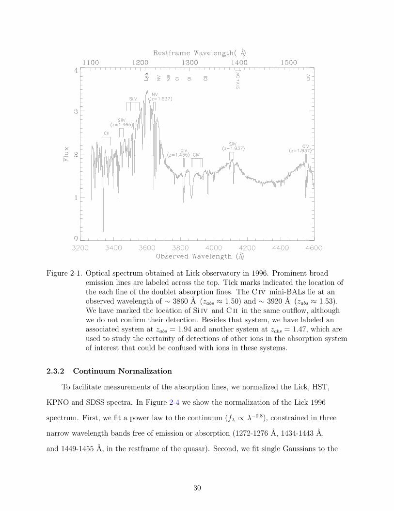
Figure 2-1. Optical spectrum obtained at Lick observatory in 1996. Prominent broademission lines are labeled across the top. Tick marks indicated the location ofthe each line of the doublet absorption lines. The C iv mini-BALs lie at anobserved wavelength of ∼ 3860 A (zabs ≈ 1.50) and ∼ 3920 A (zabs ≈ 1.53).We have marked the location of Si iv and C ii in the same outflow, althoughwe do not confirm their detection. Besides that system, we have labeled anassociated system at zabs = 1.94 and another system at zabs = 1.47, which areused to study the certainty of detections of other ions in the absorption systemof interest that could be confused with ions in these systems.

2.3.2 Continuum Normalization

To facilitate measurements of the absorption lines, we normalized the Lick, HST,

KPNO and SDSS spectra. In Figure 2-4 we show the normalization of the Lick 1996

spectrum. First, we fit a power law to the continuum (fλ ∝ λ−0.8), constrained in three

narrow wavelength bands free of emission or absorption (1272-1276 A, 1434-1443 A,

and 1449-1455 A, in the restframe of the quasar). Second, we fit single Gaussians to the

30

Figure 2-2. Ultraviolet spectrum from the HST archive (1994 and 1995 spectra combined).Prominent broad emission lines are labeled across the top. Tick marks indicatethe location of expected lines in the zabs ≈ 1.50 outflow. The strong absorptionfeature at observed wavelength ∼ 2870 A is an unrelated Damped Lyα atzabs ∼1.37. The strong Lyman Limit (LL) at a observed wavelength ∼ 2250 Acorresponds to the also unrelated absorption system at zabs ∼ 1.47

emission lines around the C iv absorption (Si ii λ1263A, O i λ1305A, C ii λ1335A, and

Si iv+O iv] λ1400A). The location of this pseudo-continuum is particularly uncertain in

the region ∼1280-1350 A in the rest frame due to the several parameters that take part

in the fitting of the weaker emission lines (Si ii, O i and C ii). We constrained our fits to

these emission lines to be redshifted by ∼ 300 km s−1 with respect to the redshift of the

stronger Si iv+O iv] feature, for which the best single-gaussian fit occurs at zem = 1.94.

This redshift agrees well with the value zem = 1.966 reported by Tytler and Fan (1992),

based on lower ionization lines (Mg ii and Lyα). We also constrained the Full Width

31

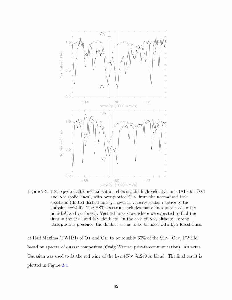
Figure 2-3. HST spectra after normalization, showing the high-velocity mini-BALs for Oviand Nv (solid lines), with over-plotted C iv from the normalized Lickspectrum (dotted-dashed lines), shown in velocity scaled relative to theemission redshift. The HST spectrum includes many lines unrelated to themini-BALs (Lyα forest). Vertical lines show where we expected to find thelines in the Ovi and Nv doublets. In the case of Nv, although strongabsorption is presence, the doublet seems to be blended with Lyα forest lines.

at Half Maxima (FWHM) of O i and C ii to be roughly 60% of the Si iv+O iv] FWHM

based on spectra of quasar composites (Craig Warner, private communication). An extra

Gaussian was used to fit the red wing of the Lyα+Nv λ1240 A blend. The final result is

plotted in Figure 2-4.

32

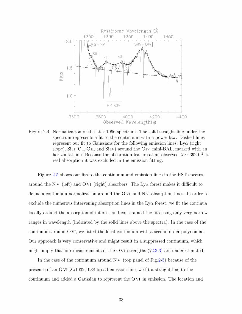
Figure 2-4. Normalization of the Lick 1996 spectrum. The solid straight line under thespectrum represents a fit to the continuum with a power law. Dashed linesrepresent our fit to Gaussians for the following emission lines: Lyα (rightslope), Si ii, O i, C ii, and Si iv) around the C iv mini-BAL, marked with anhorizontal line. Because the absorption feature at an observed λ ∼ 3920 A isreal absorption it was excluded in the emission fitting.

Figure 2-5 shows our fits to the continuum and emission lines in the HST spectra

around the Nv (left) and Ovi (right) absorbers. The Lyα forest makes it difficult to

define a continuum normalization around the Ovi and Nv absorption lines. In order to

exclude the numerous intervening absorption lines in the Lyα forest, we fit the continua

locally around the absorption of interest and constrained the fits using only very narrow

ranges in wavelength (indicated by the solid lines above the spectra). In the case of the

continuum around Ovi, we fitted the local continuum with a second order polynomial.

Our approach is very conservative and might result in a suppressed continuum, which

might imply that our measurements of the Ovi strengths (§2.3.3) are underestimated.

In the case of the continuum around Nv (top panel of Fig.2-5) because of the

presence of an Ovi λλ1032,1038 broad emission line, we fit a straight line to the

continuum and added a Gaussian to represent the Ovi in emission. The location and

33

shape of this Gaussian is based on our own judgement on selecting the constraining

narrow wavelength ranges to be fitted. We decided to take a conservative approach and

fit a weak Gaussian that, once removed, might result in some remaining emission. We

centered the Ovi emission Gaussian at a redshift zem ≈ 1.92. This redshift is consistent

with the decrement of emission redshifts at higher ionizations, comparing to the other

redshifts (1.966 and 1.939) based on lower ionization lines (Mg ii and Si iv, respectively),

mentioned before.

Similar local continua were normalized around the absorption of C iii, N iii, Si iv, Pv,

Lyα, and Lyβ.

2.3.3 Line Measurements and Physical Quantities

To extract quantitative information from the mini-BALs and broader absorbers, we

needed to fit the lines detected in the outflow. We assumed the line strengths are given by

Iv = Io(1− Cf ) + CfIoe−τv (2–1)

where Io is the intensity of the normalized continuum, Cf is the line-of-sight coverage

fraction (0 ≤ Cf ≤ 1), a measurement of the coverage of the emission source by the

absorber, and τv is the optical depth (Hamann & Ferland 1999). For simplicity due to the

medium resolution of the spectra, we have assumed that the Cf has only one value over

the whole profile. We also have assumed that the optical depths are Gaussians defined as

τv = τoe− v2

b2 (2–2)

where τo is the optical depth at the center of the line, v is the velocity and b is the

Doppler parameter. When doublet resonance lines such as C iv, Nv and Ovi are not

saturated, their oscillator strengths dictate different line strengths because the true optical

depth ratio is 2:1 for all of them.

Figure 2-6 shows the fits performed over C iv Nv, and Ovi. Thick lines represent

the final fit, which is a combination of three features (A, B, and C). We corrected for

34

Figure 2-5. Normalization of the HST spectrum (two epochs combined) around the Nvλλ1239,1243 absorption line (∼1035-1065 A, in the quasar restframe) - top -and around the Ovi λλ1032,1038 absorption line (∼ 860-890 A) - bottom.Solid lines above each spectrum represent the range chosen for the polynomialfit, which is represented by dotted lines. The continuum at the left of Nv(top) also shows a Ovi broad emission line, represented as a single Gaussianand extacted from the spectrum.

instrumental broadening Gaussian deconvolution. This has a small effect on only the

narrowest system A. Features A and B were detected in the C iv absorption and are

present in Ovi and Nv as well, while a C component of the absorption seems to

be present in Ovi and Nv, but not in C iv. Because C iv lies in a region free from

contamination with Lyα lines, we used, as a first approximation for the fits of the features

35

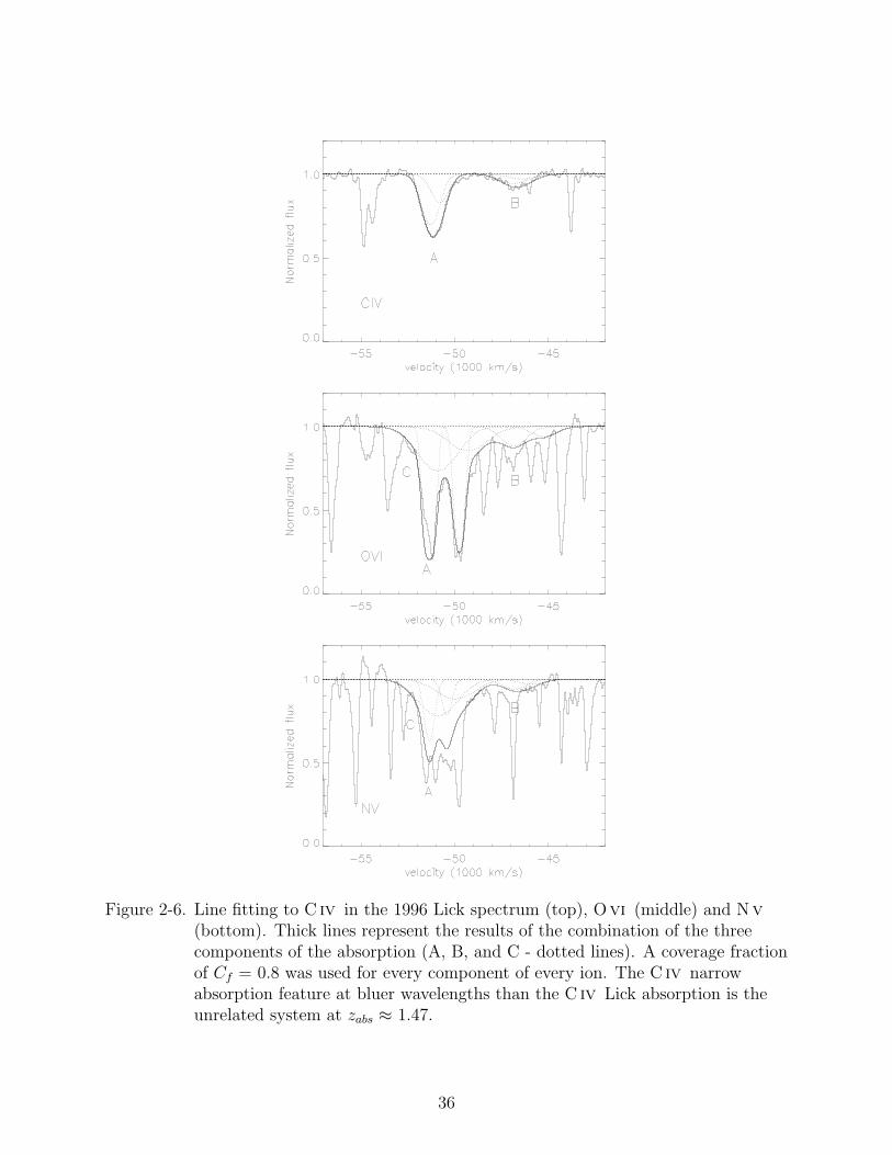
Figure 2-6. Line fitting to C iv in the 1996 Lick spectrum (top), Ovi (middle) and Nv(bottom). Thick lines represent the results of the combination of the threecomponents of the absorption (A, B, and C - dotted lines). A coverage fractionof Cf = 0.8 was used for every component of every ion. The C iv narrowabsorption feature at bluer wavelengths than the C iv Lick absorption is theunrelated system at zabs ≈ 1.47.

36

A and B in Ovi and Nv, the redshift and FWHM of the features A and B in C iv.

In particular, we fit feature B in C iv and used it as a template in Ovi and Nv, only

allowing for changes in τo. However, another broader component (C) seems to be present

both in Ovi and Nv, while it is apparently non-existent in C iv. We used the parameters

resulting from the Ovi fit of the feature A and C to construct the Nv fit because of

the presence of many Lyα lines blended with the Nv absorption did not allow us to

perform an actual fit, especially over the A feature. Note that the features A, B and C are

defined for convenience only for the the HST and Lick 1996 data sets. The multi-epoch

observations across C iv show that the character of the absorption changes significantly.

In particular, A, B and C lose their identity altogether in the later SDSS and KPNO

spectra as we will discuss later while describing their variability. The variability and

absorbers kinematics will be discussed in section §2.4.2.

Figure 2-6 shows that the two strong narrow components of Ovi seem to be present

in a ∼1:1 depth ratio, characteristic of saturated profiles, although saturation is not

occurring at zero flux. Since the profiles are resolved (FWHM > 150 km s−1), this

indicates partial coverage of the background emission source (i.e., the emission source is

not completely covered by the outflow in our line of sight, Hamann & Ferland 1999). We

obtain a value of Cf ' 0.8 for Ovi. Since feature A in Ovi is the only feature and ion

where we can distinguish both lines in the doublet, we used this value for all the other

ions, although we are aware of other studies where it has been found that Cf may vary

from ion to ion (Hamann et al. 1997c) and that the C iv, in particular, could have any

value from 1 to 0.4 since it was not observed simultaneously with the HST data. We also

include measurements based on Cf = 1 in Tables 2-2 and 2-3 for comparison.

Table 2-2 includes the results for Cf (v) = 1 and 0.8. Values for the Rest Equivalent

Width (REW) are derived by integrating over the fitted profile, combining all of the

components that are present (thick solid lines in Figure 2-6). The errors in REW are

derived by varying the continuum to the highest and lowest possible continuum based

37

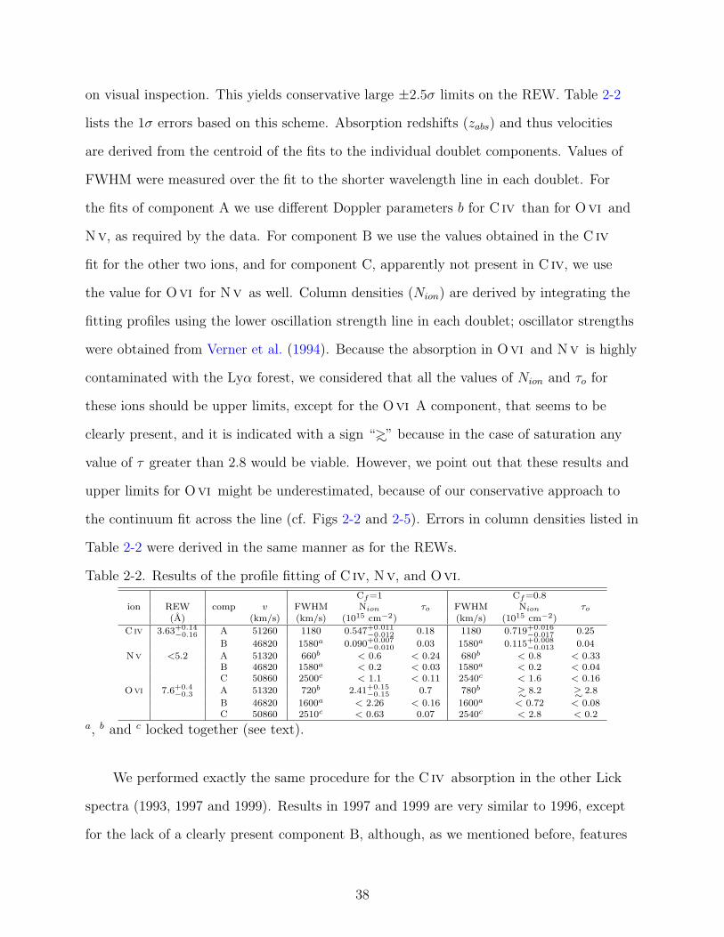
on visual inspection. This yields conservative large ±2.5σ limits on the REW. Table 2-2

lists the 1σ errors based on this scheme. Absorption redshifts (zabs) and thus velocities

are derived from the centroid of the fits to the individual doublet components. Values of

FWHM were measured over the fit to the shorter wavelength line in each doublet. For

the fits of component A we use different Doppler parameters b for C iv than for Ovi and

Nv, as required by the data. For component B we use the values obtained in the C iv

fit for the other two ions, and for component C, apparently not present in C iv, we use

the value for Ovi for Nv as well. Column densities (Nion) are derived by integrating the

fitting profiles using the lower oscillation strength line in each doublet; oscillator strengths

were obtained from Verner et al. (1994). Because the absorption in Ovi and Nv is highly

contaminated with the Lyα forest, we considered that all the values of Nion and τo for

these ions should be upper limits, except for the Ovi A component, that seems to be

clearly present, and it is indicated with a sign “∼>” because in the case of saturation any

value of τ greater than 2.8 would be viable. However, we point out that these results and

upper limits for Ovi might be underestimated, because of our conservative approach to

the continuum fit across the line (cf. Figs 2-2 and 2-5). Errors in column densities listed in

Table 2-2 were derived in the same manner as for the REWs.

Table 2-2. Results of the profile fitting of C iv, Nv, and Ovi.

Cf=1 Cf=0.8ion REW comp v FWHM Nion τo FWHM Nion τo

(A) (km/s) (km/s) (1015 cm−2) (km/s) (1015 cm−2)

C iv 3.63+0.14−0.16 A 51260 1180 0.547+0.011

−0.012 0.18 1180 0.719+0.016−0.017 0.25

B 46820 1580a 0.090+0.007−0.010 0.03 1580a 0.115+0.008

−0.013 0.04

Nv <5.2 A 51320 660b < 0.6 < 0.24 680b < 0.8 < 0.33B 46820 1580a < 0.2 < 0.03 1580a < 0.2 < 0.04C 50860 2500c < 1.1 < 0.11 2540c < 1.6 < 0.16

Ovi 7.6+0.4−0.3 A 51320 720b 2.41+0.15

−0.15 0.7 780b∼> 8.2 ∼> 2.8

B 46820 1600a < 2.26 < 0.16 1600a < 0.72 < 0.08C 50860 2510c < 0.63 0.07 2540c < 2.8 < 0.2

a, b and c locked together (see text).

We performed exactly the same procedure for the C iv absorption in the other Lick

spectra (1993, 1997 and 1999). Results in 1997 and 1999 are very similar to 1996, except

for the lack of a clearly present component B, although, as we mentioned before, features

38

A, B and C lose their identity as time evolves. Variability will be discussed further in

§2.4.2.

As noted above (see section 2.3.1), we do not clearly detect absorption in C iii,

N iii, Pv, Si iv, Lyα or Lyβ, at the redshift of the C iv, Nv and Ovi absorbers. All of

these features lie in the Lyα forest and in every case there is some absorption present.

Therefore, we outlined absorption profiles for component A in the blue-shifted wavelengths

of these ions to place upper limits on the column densities and set limits on the absorber

ionization. We use the same zabs and b parameters as in Ovi (for lines found in the HST

spectra) and C iv (for the lines in the Lick spectra) for the A component and increase

the strength of the line (τ) until it was obviously much stronger than the data at the

wavelengths of interest. Figure 2-7 shows examples of these upper limits and Table 2-3

includes the results.

Table 2-3. Upper limits on lines not detected

Cf=0.8ion REW (A) Nion (1015 cm−2)C iii < 1.3 < 0.36N iii < 0.4 < 0.55Pv < 0.5 < 0.09Si iv < 1.7 < 0.17Lyα < 1.6 < 0.5Lyβ < 0.8 < 1.57

We can also place an upper limit for the edge at the Lyman limit in this system

(which is definitely not very strong - see Figure 2-2). The small decline of the continuum

corresponds to an optical depth τLL ∼< 0.2.

2.4 Discussion

2.4.1 Ionization and Total Column Density of the Outflow

To study the physical properties of these clouds we analyze their degree of ionization,

which is quantified by the ionization parameter, U , the dimensionless ratio of

hydrogen-ionizing photon to hydrogen space densities at the illuminated face of the

cloud. We constrain its value from different approaches.

39

Figure 2-7. Upper limits to absorption lines for C iii (top left), N iii (top right) and Pv(bottom) based on component A only in C iv in the 1996 Lick spectrum.

Hamann & Ferland (1999) presented results of theoretical ratios of column densities

for different ions calculated by CLOUDY photoionization simulations in photoionized

clouds that are optically thin in the Lyman continuum. We used these results (as shown in

their Figure 10) to estimate U from the theoretical ratios of column densities for different

ions of the same element (such as C iii and C iv) and for different elements (such as C iv

and Ovi), assuming solar abundances (Grevesse & Sauval 1998).

We estimated U to be log U ∼> -1.1 for both components A or B, from the ratio

between N(C iv) and N(Ovi), using Cf = 0.8 (where N(Ovi) is a lower limit - see section

§2.3.3 for comments on column densities). We also calculated a limit on U from the ratio

of column densities of component A in C iv and C iii, N(C iv)/N(C iii) ∼> 2, from which

we obtain another lower limit of log U ≥ −2.2, which is less restrictive than the previous

40

one. Obtaining such a high ionization, we do not expect to find many low ionization lines.

From the remaining of this discussion we will use the value of log U ∼> -1.1.

If the metalicity (O/H) is solar and the ionization maximizes the amount of Ovi,

such that N(Ovi)/N(O)≈ 0.4 at log U = -1.0 (see Figure 10 from Hamann & Ferland

1999), we can estimate a total column density (NH) as follows:

NH =N(H)

N(O)

N(O)

N(OV I)N(OV I) (2–3)

which yields the value NH ∼> 3.0 x 1019 cm−2 (using only component A). This value is a

lower limit both because N(Ovi) is a lower limit (Table 2-2) and because the actual ratio

N(Ovi)/N(O) might be smaller. Super-solar metallicities, as reported in high redshift

quasars (Dietrich et al. 2003), might decrease this NH limit by factors of a few.

The upper limit on the Lyα column density (see Table 2-3) can be used to derive a

lower limit on U : log U ∼> -0.6. The absence of a Lyman edge is consistent with this limit.

The value of log U ∼> -0.6 is somewhat larger than the Ovi result of log U ∼ -1.1. This

higher ionization in Equation 2–3 would also lead to a larger NH limit, which could be

mitigated somewhat by higher metallicities. However, it appears overall that our estimates

of log U ∼> -1.1 and NH ∼> 3.0 x 10 19 cm−2 are firm lower limits and are consistent with

the non-detections of other low to moderate ionizations lines such as C iii and Si iv.

2.4.2 Nature of the Absorber, Variability and Kinematics

Strong C iv and Ovi absorption are clearly present at zabs ≈ 1.50, and they appear

to be accompanied by strong (but blended) Nv absorption. The high-velocity absorption

profiles are complex and highly variable. Multi-epoch observations across the C iv feature

(see also Narayanan et al. 2004 and below in this section) show variable absorption across

a velocity interval of at least 45000 to 54300 km s−1 relative to the emission redshift

derived from low ionization lines (zem = 1.966). In the 1996 spectrum we identify distinct

mini-BALs in C iv that we labeled A and B (Figure 2-6). However, these features evolve

and lose their identities altogether in subsequent observations. Although the velocity

41

centroid and deepest part of the C iv trough shifts between observations, there is no clear

evidence for acceleration or deceleration in the outflow.

A comparison of the C iv and Ovi lines in 1994/1995(HST)–1996(Lick) also suggests

further that the absorber has an ionization dependence. In particular, the Ovi absorption

includes a broad feature (component C with FWHM ∼ 2500 km s−1) that is not present

in C iv and the narrow component (A) is considerably narrower in Ovi (FWHM ∼ 750

km s−1) than it is in C iv (FWHM ∼ 1200 km s−1). These differences might be affected

by the line variabilities since the spectra were taken at different observation times (∼1.5 month separation in the quasar time restframe). However, we note that the Ovi

absorption did not change significantly between the two HST observations in 1994 and

1995, and the C iv line measured from 1993 to 1996 had a consistently broader component

A and no very broad component C.

The C iv (measured in the 1996 spectrum), and maybe the Ovi and Nv lines

also have absorption at lower velocities (component B in Figure 2-6), better matched

by absorption profiles with v ∼ 47000 km s−1 (zabs ∼ 1.53). The later evolution of this

feature (see Figure 2-8) suggests that it might be real absorption. Note again that the Nv

absorption profile is severely contaminated by Lyα forest lines, but its overall appearance

is consistent with the Ovi mini-BALs.

Our best estimate for the Coverage Fraction is Cf = 0.8. This value was derived from

the mild saturation of the component A in the Ovi ion, as the data suggests. None of

the other components in Ovi and in the other ions allowed for a determination of the Cf

because both components of the doublet are blended together or with Lyα forest lines.

There is still some uncertainty in this result due to possible blending with Lyα forest lines.

However, the features we attribute to Ovi have the correct doublet separation, nearly the

same FWHMs and they appear at essentially the same redshift as component A measured

in C iv. The Ovi absorption occurs at wavelengths away from the broad emission lines

and therefore the absorber must partially cover the quasar continuum source.

42

Repeat observations of the C iv line show that all of these absorption components

are highly variable (see Figure 4 in Narayanan et al. 2004). More recent data (provided

by the Sloan Digital Survey Sky Survey - SDSS- and observed at the Kitt Peak National

Observatory - KPNO) shows that the variability has continued. Figure 2-8 compares the

Lick spectra in 1996, used in the analysis in this work, to the newer SDSS spectrum

obtained in 2003 and KPNO spectrum obtained in Jan 2007. The most dramatic

variability occurs between 1999 and 2003. The SDSS 2003 spectrum shows that the

absorption profile identified as A in the 1996 spectrum in Figure 2-6 has almost completely

disappeared and the absorption identified as B has increased in strength and width. The

complexity of the absorption profile in 2003 and 2007 suggests that A and B absorptions

are intertwined and thus it does not have a clear meaning to use them to identify the

profiles in the spectra beyond 1999. Between 2003 and 2007, the absorption remains

quite similar in strength, and we would like to note only a change in the maximum depth,

which shifts from v ∼ 47000 km s−1 in the 2003 spectrum to v ∼ 49000 km s−1 in the

2007 one. Similar shifts in the centroid velocity were reported between the previous Lick

observations in Narayanan et al. (2004).

2.4.3 Origin of the Outflow, Timescales and Causes for Variability

The combined properties of broad smooth absorption troughs, line variability on

time scales ≤ 1 yr in the quasar rest frame, and extremely small clouds implied by partial

covering of the quasar continuum source strongly suggest that the high velocity absorption

forms in an outflow very near the quasar (see also Hamann et al. 1997c and Hamann

& Simon 2009). The variability times, in particular, provide direct constraints on the

absorber location. If the flow is photoionized and the line changes are caused by changes

in the ionizing flux, then the recombination time sets an approximate lower limit on the

outflow gas density (see Hamann et al. 1995 and Hamann et al. 1997c). The smallest

variability time we measure in C iv, ∼ 1 yr in the quasar rest frame, corresponds to a

minimum electron density nH ∼> 1.1 x 105 cm−3. This, in turn, yields a maximum distance

43

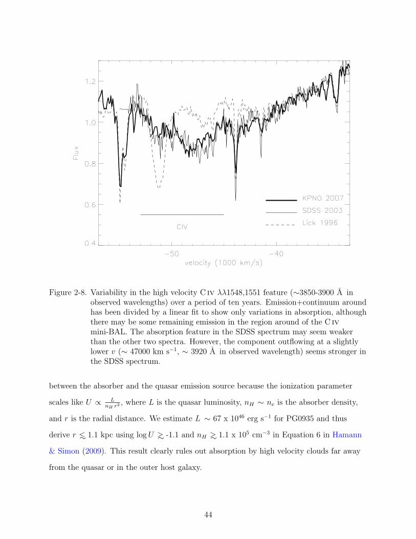
Figure 2-8. Variability in the high velocity C iv λλ1548,1551 feature (∼3850-3900 A inobserved wavelengths) over a period of ten years. Emission+continuum aroundhas been divided by a linear fit to show only variations in absorption, althoughthere may be some remaining emission in the region around of the C ivmini-BAL. The absorption feature in the SDSS spectrum may seem weakerthan the other two spectra. However, the component outflowing at a slightlylower v (∼ 47000 km s−1, ∼ 3920 A in observed wavelength) seems stronger inthe SDSS spectrum.

between the absorber and the quasar emission source because the ionization parameter

scales like U ∝ LnH r2 , where L is the quasar luminosity, nH ∼ ne is the absorber density,

and r is the radial distance. We estimate L ∼ 67 x 1046 erg s−1 for PG0935 and thus

derive r ∼< 1.1 kpc using log U ∼> -1.1 and nH ∼> 1.1 x 105 cm−3 in Equation 6 in Hamann

& Simon (2009). This result clearly rules out absorption by high velocity clouds far away

from the quasar or in the outer host galaxy.

44

However, the complex velocity-dependent variations that we observe might be difficult

to explain by simple changes in the ionizing flux. The line changes could also be caused by

clouds moving across our lines of sight to the continuum sources (see also Hamann et al.

2008). In that case, the transverse velocities (perpendicular to our sightlines) must be

large enough to cross a significant portion of the far-UV emission source in a variability

time. Specifically, the smallest observed variability time, ∼ 1 yr, and the continuum region

diameter, ∼0.003 pc at 1550 A, require transverse velocities vtr ∼> 2900 km s−1. These

velocities are similar to disk rotation speeds beyond the radius of the C iv BEL region

RCIV (vtr ∼ 3000 km s−1), and therefore this scenario is plausible.

We cannot establish whether the outflow was launched in an inner or outer region

compared to the Broad Emission Line Region (BELR). However, during these (at least)

4.7 years, the outflow has travelled over a region larger than the size of the BELR; thus

even if launched inner to it, the ouflow should be outside of it at the present time. We

estimate the RCIV to be ∼ 5 x 1017 cm from a bolometric luminosity Lbol ∼ 67 x 1046

erg s−1) derived from the observed flux at restframe 1450 A(Lλ(1450A) = 7 x 10−12 erg

s−1 cm−2), using a cosmology with Ho = 71 km s−1 Mpc, ΩM = 0.27, ΩΛ = 0.73 and

a standard bolometric correction factor of L ≈ 3.4λLλ(1450A). Because the velocity

seems to have remained constant, we can derive a flow time to travel the RBELR of

tf ∼ RCIV/v ∼ 3.5 years, shorter than the restframe timescale during which this outflow

has remained present.

The parameters obtained for the flow are consistent with radiative acceleration.

We can use the approach described in Hamann (1998), who derives the launch radius

by integrating the motion equation for a radiative pressure driven wind from an initial

“launch” radius to infinity with a certain terminal velocity. We obtain a launch radius in

this case of Rlaunch ≈ 70 pc for PG0935+417. Note that the equation in Hamann (1998)

requires the use of a fraction of the spectral energy distribution absorbed or scattered in

the wind. We have assumed fL ≈ 1 because it is the typical value for BAL flows (Hamann

45

1998). However, this parameter may be smaller for winds with narrower lines such as the

mini-BAL in PG0935+417. If instead of absorbing 10% of the radiation the outflow only

absorbs 5%, the launch radius would decrease by ∼50%. These results are consistent with

radiation pressure powering this outflow.

Is PG0935+417 special? In spite of its extreme speed, as long as fL is not too

small, the flow can be launched within 70 pc of the continuum source and accelerated by

radiation pressure. However, the actual physical processes that could produce a flow like

this are not understood. Observationally, we know that flows with speeds v > 50000 km

s−1 are rare - much rarer than flows with v < 25000 km s−1, for example (see Chapter 3).

As it seems, we do not need to invoke a very small radius to launch this outflow. Then, if

it is easy to launch these high velocity outflows, they should be a common phenomenon in

quasars. However, as reported in Chapter 3 we find outflows at v > 25000 km s−1 in 2.5%

of optically selected quasars. The luminosity in PG0935+417 is not close to the Eddington

Luminosity (LEdd). Since MBH ∼ 3 x 1010 M¯, we obtain a L/LEdd ∼ 0.2. Therefore, more

than a special particularity of this individual quasar, we conclude that, considering that

the statistical sample in Chapter 3 is observed from every angle, the “angle of sight” of

these high velocity absorbers must be narrow to only appear in 2.5% of the cases.

X-ray observations are needed to constrain better the total absorbing column and

examine the relationship of this high-speed outflow to the stronger but generally lower

velocity BALs.

2.5 Conclusion

Energetic outflows are common phenomena in AGNs that could help us understand

the mechanisms that power the central regions of these luminous engines. Outflows

are observed in the spectra of quasars as blueshifted absorption lines. I present new

measurements and analyses of these absorption lines in the spectra of the quasar

PG0935+417 (zem ≈ 1.966). This quasar shows a high velocity C iv mini-Broad

Absorption Line (mini-BAL) outflowing at ∼51000 km s−1. We detect, using Lick

46

observatory, Hubble Space Telescope, and Sloan Digital Sky Survey spectra, absorption in

C iv λλ1548,1551 (already reported in Hamann et al. 1997a and Narayanan et al. 2004)

and, for the first time in this outflow, in Nv λλ1240 and Ovi λλ1034 in this mini-BAL

system. The absence of lower ionization lines indicates that the flow is highly ionized

with an ionization parameter log U ∼> -1.1. The resolved Ovi indicates that the lines are

moderately saturated with the absorber covering just ∼80% of the background continuum

source. We estimate the total column density to be NH ∼> 3.0 x 1019 cm−2, which is small

enough to be compatible with radiation pressure mechanisms accelerating this outflow.

47

CHAPTER 3AN INVENTORY OF C iv MINI-BALS AND OUTFLOW LINES IN SDSS QUASARS

3.1 Introduction

A first step towards comprehending better the nature of quasar outflows requires

a complete inventory, without pre-selections based on BI, AI, FWHM or velocity. To

compile such a catalog, we initiated a program to produce a complete catalog of all

C iv λλ1548,1551 absorption lines in optically selected quasars from the Sloan Digital

Sky Survey (SDSS) Data Release 4 (DR4). We examined the 2200 brightest quasars at

redshifts z ∼ 2 that, due to the SDSS wavelength coverage, allowed us to identify and

measure every available C iv λλ1548,1551 absorption line in the SDSS quasar spectra.

In Nestor et al. (2008), we presented a statistical study on the C iv outflows observed

as narrow absorption lines (FWHM < 600 km s−1) to exclude the more obvious outflow

lines. In Nestor et al. (2008) we concluded that a significant number of narrow absorption

lines (≥43%±6%), in the velocity range 750 km s−1 ∼< v ∼< 12000 km s−1 and with Rest

Equivalent in the C ivλ1548 line (REWλ1548)>0.3 A, are quasar outflows. In the present

work we study the C iv absorption lines detected as broader absorption (FWHM ≥ 600

km s−1) with the goal of identifying individual outflow absorbers and characterizing their

frequency. Due to the SDSS resolution, blends of intervening narrow lines, could appear

as broader absorption lines. Thus, it is necessary to set a threshold to discard these

intervening absorption lines. In Section 3.4 we explain how we select a high-confidence

zone of the FWHM space where we have excluded the intervening absorption.

Our analysis emphasizes the mini-BALs because they are the least studied class to

date. However, the goal of this chapter is to characterize outflows in a more general way,

as we include BALs in this analysis as well. The information regarding v, width, and

strength allows us to study whether different classes of absorption lines are more or less

frequent at different velocities, and whether or not they coexist in the same line of sight.

Also, we study the frequency of outflows at high velocities (v ∼> 25000 km s−1), up to Lyα,

48

which is probably the bluest-possible detection of C iv at these redshifts because the Lyα

forest likely produces ambiguous C iv identification in the shortward of the Lyα emission

line.

This chapter starts by introducing the sample we used (§3.2) and how the catalog

of C iv outflows was developed (§3.3). In §3.4 we introduce a working definition for

mini-BALs and in §3.5 we discuss their frequency of occurance in quasar spectra and

their relation to the frequency of other types of absorption features (BALs, AALs, Mg ii),

and the quasar radio properties. Finally, we summarize the main results of this work and

discuss some implications for the overall study of quasar outflows (§3.6).

3.2 Quasar Sample

We examined 2210 quasar spectra from the SDSS Data Release 4 (DR4). The

data span a wavelength range of 3820 A (with resolution R = 1800) to 9200 A (with

R = 2100). In order to study the incidence of high velocity C iv λλ1548,1550 absorption

outflowing with at least v ∼ 30000 km s−1 in quasar rest frame velocity space, we

selected quasars with quasar redshift zem ≥ 1.8. To study the distribution of narrow

C iv absorbers near the quasars (Nestor et al. 2008) we needed accurate measures of the

quasar redshifts. SDSS quasar redshifts are calculated using automated algorithms. To

determine more accurate velocity zero-points by using the Mg ii λλ2796,2803 emission

lines, which required a maximum SDSS quasar redshift of 2.25, we examined the ∼1000

brightest quasar spectra (with the highest median S/N in the r-band, ≥17.9) with 1.8

≤ zem ≤ 2.25. We supplemented this sample for two different reasons. First, to study

the incidence of absorption lines at relatively low quasar-frame velocity (results reported

in Nestor et al. 2008), we added 500 quasar spectra with 1.6≤ zem ≤ 1.8 (r-band S/N

≥18.7). Second, to study the incidence of absorption lines at very high velocity (v ≥ 30000

km s−1 and up to 60000 km s−1), we supplemented the sample with 700 quasar spectra

with zem ≥ 2.14 (r-band S/N≥17.1). Precise zero-point velocity determinations are not a

concern when studying these high-velocity absorption lines. Although accurate velocity

49

zero-points are not crucial for the analysis carried out in this chapter, we benefited from

the zem measurements from Nestor et al. (2008) when available.

Visual inspection revealed that some objects were misidentified stars; those were

rejected, resulting in 2200 spectra with zem ≥ 1.6 that comprised our final sample.

3.3 Identification and Measurements of C iv Absorption Lines

With the goal of producing the first systematic account of C ivλλ1548,1550 outflows

in quasar spectra, we identified and measured every C iv doublet in every quasar spectrum

in the sample described in §3.2.

We fit pseudo-continua using a cubic spline function for the underlying continuum

and one or more Gaussians for the broad emission lines to each quasar spectrum, and

flagged C iv absorption candidates in a manner identical to that described in Nestor et al.

(2005), but using updated versions of the software, adjusted to suit the C iv doublet

(Nestor et al. 2008). Each continuum fit and detected candidate was visually inspected. In

order to avoid “fitting-out” smooth broad absorption and missing very shallow absorption,

and to check that the software was identifying good power law continua, we inspected the

region covered from Lyα1216 A to ∼1700 A. We verified the production of a good local

continuum around absorption lines, marked whenever it was uncertain, and eliminated

redundant and spurious detections; the continuum fitting sometimes produced probable

false-positive broad absorption lines, and we marked as questionable cases those where the

presence of absorption was ambiguous. The blended Lyα+Nv λλ1239,1243 emission lines

sometimes presented problems for the continuum-fitting software. To avoid potential errors

we excluded these regions (v ∼> 60000 km s−1) from the analysis. In the case of narrow

absorption lines where both components of the doublet are resolved and distinguishable,

the software requires the correct doublet separation of ∆v ∼500 km s−1. In the case of

broad absorption lines (where individual lines of the doublet are not distinguishable), we

let the software select every absorption trough and verified that the C iv identification was

correct, excluding any ambiguous cases. For example, the sometimes present gap between

50

the doublet Si ivλλ1394,1403 and the doublet O iv]λλ1397,1400 emission lines (v ∼30000 km s−1) could be mistaken for absorption, and therefore we excluded absorption

candidates from this region unless they were wide or strong enough to not likely be

explained by separation between the emission lines, cases that we marked down also as

questionable. In a similar way, we rejected or marked as questionable those candidates at

v ∼ 40000–50000 km s−1 due to the sometimes present combination of O iλ1305A and

C iiλ1335A emission lines, although their effect is less pronunced than for Si iv+O iv],

since O i and C ii are not always present. Also, we excluded cases where C iv could

be identified as Si iv. C iv is the most common ion in the region searched, but Si iv

sometimes is present whenever C iv is at the same zabs. We let the software select every

absorption trough and, in the case of broad absorption, we excluded the cases that could

be identified as Si iv. All these exclusions could partly account for the scarcity of detected

absorption lines in certain velocity ranges.

In our sample we found 26 BALs that were strong enough to make continuum

determination and absorption measurement too complicated – we flagged them as BALs

but did not determine their continua or fit any absorption lines.

We then fit every detected C iv absorption line to measure their width (FWHM),

radial velocity centroid (v) and REW. Gaussian line profiles were satisfactory for our

purposes since they produce good measurements of those parameters. Therefore, we

designed IDL software that fit a Gaussian line profile pair, using a Levenberg-Marquardt

least-squares fit, to the C iv doublet absorption lines. Each C iv doublet line was

constrained to have the same FWHM and v, the correct C iv doublet separation

(∆v ∼500 km s−1), and a λ1548.2 : λ1550.77 intensity ratio constrained to the range

1:1 to 2:1 within the noise. In most cases, the Gaussian profile resulted in an excellent fit;

we noted cases where the absorption profile shape deviated from the Gaussian fit such that

the measurements of FWHM and REW were not completely accurate.

51

Most of the detected doublets were narrow enough that the individual lines of

the doublet were not blended with each other, and were not blended with transitions

from absorption at other redshifts. In some cases, the C iv doublets blended with the

intervening doublet Mg ii λλ2796,2803. Thus, we added a tool in the software to fit the

Mg ii doublet simultaneously with the C iv doublet and remove it from the C iv fit. In

the rare case of blending with other ions, we allowed the software to skip the other ion

line. However, the relatively large incidence of C iv absorption, especially at zabs ∼ zem,

occasionally leads to multiple systems blending together. Then, we allowed the software

to fit multiple pairs of Gaussians to the absorption profiles. In some cases, this blending

caused an ambiguity in the number of doublet pairs to use in the fitting. In all cases,

we used the minimum number of doublet pairs “necessary” to reproduce the observed

number of components. Also, we relied, when available, on the presence of other ions with

the same ionization (Si iv, Nv, etc.) at the same redshift to help determine the correct

number of C iv absorption lines within the blends. In the case of narrow components,

“necessary” meant that both lines of the doublet needed to be clearly present. We fit

broad absorption lines blended together with several Gaussians whenever the trough

shape strongly suggested multiple components. To analyze possible de-blending issues, we

included a comment about the cases that we split into several absorption lines but could

be part of blended systems.

This procedure resulted in the measurement of 5321 C iv absorption lines. Figure 3-1

shows the velocity distribution of all C iv absorption. The lower plot shows the number

of quasars contributing to each velocity, which starts to decrease beyond v ∼16000 km

s−1. The large number of narrow absorption lines is mostly due to intervening systems,

but the fraction of intrinsic NALs is significant (e.g., Nestor et al. 2008). The deficit of

absorption at velocities ∼30000 km s−1 and ∼40000-50000 km s−1 is partly due to the

fewer spectra available at those velocity ranges and the aforementioned presence of the

52

Si iv+O iv]λ1400 emission line and the sometimes present combination of O iλ1305A and

C iiλ1335A emission lines, respectively.

Figure 3-1. Top: Distribution of all the absorption systems measured in FWHM-velocityspace (crosses). We have included the cases marked down as questionable aswell (circles). Most of these cases fall around emission line regions, since it isdifficult to decide whether a system is real absorption when it lies between twoclose emission lines. The presence of the Si iv+O iv]λ1400 emission line affectsthe detectability of systems and produces a probably artificial reduction ofC iv absorption at velocities of ∼30000 km s−1. Similar effects, although lessnotorious since they are less abundant, are produced by the O iλ1305A andC iiλ1335A emission lines at ∼40000-50000 km s−1. Bottom: Number ofquasars covering each velocity range. Note that the y-axis ranges upward from500 quasars. Every quasar spectrum covers up to 16000 km s−1, but only halfof them cover up to 60000 km s−1.

Table 3-1 lists the measurement results for every C iv absorption line with FWHM

≥ 600 km s−1. We performed this initial cutoff with the goal of studying outflow systems

and knowing that narrower ones have an uncertain origin. We carried out a statistical

53

study of the absorption lines with FWHM < 600 km s−1 in Nestor et al. (2008). Table

3-1 includes measurements of REW (for C ivλ1548 and C ivλ1550 doublet lines, called

REWλ1548 and REWλ1550 respectively), FWHM, v and zabs as well as magnitude r, zem, BI

and AI, introduced in Chapter 1 and explained in the paragraphs below. Table 3-1 also

includes a column with comments for cases where 1) the C iv absorption identification

is questionable (“q”), 2) the correct location of the continuum fit might be questionable

but the C iv absorption is definitely present (“c”), 3) the Gaussian fitting results in a

poor fit (“f”) and therefore measurements of FWHM and REW are approximate, and 4)

deblending could cause double-counting of absorption (“b”). Figure 3-2 includes examples

of absorption marked with some of these comments.

We also looked for strong Lyα absorption lines at the same redshift as the C iv lines,

which is characteristic of Damped Lyα and Lyman limit systems, at the same redshift

of every C iv absorption line analyzed. Our purpose is merely to exclude them from the

analysis of this chapter since they are not likely to be part of quasar outflows. The 11

cases we found were, however, included in Table 3-1 for future reference. They are labeled

as “d”, when a strong Lyα absorption line was present, or “d2” when the Lyα was present

but not very strong, or zabs ∼< 2.15 so we were not able to inspect the corresponding Lyα

absorption line region, but some other low ionization ions at the same zabs as C iv were

present (Mg ii λλ2796, 2804 and Al ii λ1671, some or all of the iron lines Fe ii λ1608,

2344, 2374, 2383, 2587, 2600 and sometimes Si ii λ1527), which pose some risk of being

a Damped Lyα or Lyman limit system. Cases where only Mg ii or Al iii were present

but no other low ionization ions were detected, and thus the C iv absorption is unlikely

to be part of a Damped Lyα or Lyman limit system, were included in the analysis and

commented in Table 3-1 with the designations “Mg ii” and/or “Al iii”.

Besides the individual absorption characteristics, Table 3-1 includes also some

characteristics of the overall quasar spectra: zem, BI and AI. For zem we include the SDSS

and Nestor et al. (2008) values, when available. We computed measurements for the BI

54

Figure 3-2. Examples of different fits and their comment-codes in Table 3-1. ‘c’ is acandidate where the Continuum fit is debatable but the C iv absorption isreal. ‘f’ is a poor fit that might result in bad measurements of FWHM andREW. ‘b’ is an absorption line that has been deblended and could beconsidered part of a blend with absorption in the proximity.

and AI for each quasar, using the definitions included in the introduction of this chapter.

We allowed for three consecutive instances of noise spikes before resetting the value of C

to 0. When the spectral velocity coverage did not reach 25000(/29000) km s−1, then the

value of BI(/AI) is a lower limit, and the value of BI(/AI) is followed by a “*” in Table

3-1. Note that the zero velocity in BI is defined using the average wavelengths of the

C iv doublet, while in AI it is defined using the longest wavelength line of the doublet:

1550.77 A. We do not include a formal error to either BI or AI because the uncertainties

are dominated by the determination of the continuum. The measurements of BI and AI

depend to a large extent on the continuum placement, and normal differences are expected

55

between our method that uses a cubic spline function, versus those that used templates

derived from composites.

Table 3-2 lists the 26 BALs for which continua were not normalized and therefore we

did not perform any C iv absorption line detection and fitting. They were classified as

BALQSOs with BI larger than 2000 km s−1.

56

Tab

le3-

1.Lis

tof

min

i-B

ALs

Qua

sar

rz e

mz e

mB

IA

Iz a

bs

vFW

HM

RE

Wλ1548

RE

Wλ1550

com

men

t(m

ag)

(Mgii)

(km

s−1)

(km

s−1)

(km

s−1)

(km

s−1)

(A)

(A)

J000

103.

85-1

0463

0.31

18.3

72.

082.

070

769

2.05

2086

1072

2.08

92.

093

J001

710.

86+

1355

56.5

217

.90

1.81

1.81

00

1.82

-113

764

30.

317

0.15

9q

J002

127.

88+

0104

20.2

018

.64

1.82

1.82

454

984

1.79

4170

1698

4.03

04.

037

J002

342.

98+

0102

43.0

018

.44

1.64

1.64

54*

497*

1.57

8063

1958

2.37

71.

194

J002

710.

06-0

9443

5.37

18.2

62.

072.

0882

216

542.

0349

2715

274.

877

4.88

6J0

0350

3.76

+00

1641

.70

17.9

82.

67...

.0

272.

5780

4217

151.

114

0.56

0J0

0461

3.54

+01

0425

.74

18.0

32.

15...

.41

4276

371.

9718

254

2275

2.54

42.

548

c,b

J004

613.

54+

0104

25.7

418

.03

2.15

....

4142

7637

2.01

1373

938

8810

.647

10.6

65c,

bJ0

0461

3.54

+01

0425

.74

18.0

32.

15...

.41

4276

372.

1230

2730

139.

986

8.90

2c,

fJ0

0540

8.46

-094

638.

1517

.78

2.13

2.12

973

1512

2.06

6059

2628

5.35

85.

367

cJ0

0541

9.99

+00

2728

.01

18.3

12.

52...

.11

761

52.

3217

706

1900

1.01

31.

017

cJ0

0541

9.99

+00

2728

.01

18.3

12.

52...

.11

761

52.

4191

3228

452.

453

1.23

5c

J005

951.

67-0

8442

3.88

18.2

22.

142.

150

1011

2.13

1954

828

2.94

52.

884

J011

605.

97+

1334

02.1

718

.32

2.01

2.01

972

2833

1.81

2073

727

244.

496

4.53

5J0

1160

5.97

+13

3402

.17

18.3

22.

012.

0197

228

331.

9916

9918

595.

441

5.45

0c

J012

231.

91+

1339

40.8

418

.24

3.06

....

4667

5356

2.89

1346

039

887.

056

7.39

5b

J012

231.

91+

1339

40.8

418

.24

3.06

....

4667

5356

2.92

1077

820

713.

758

3.76

4b

J012

231.

91+

1339

40.8

418

.24

3.06

....

4667

5356

2.97

6820

774

2.09

51.

294

cJ0

1223

1.91

+13

3940

.84

18.2

43.

06...

.46

6753

562.

9956

7479

72.

246

2.25

0c

J014

809.

65-0

0101

7.84

17.9

52.

162.

170

01.

6948

085

2529

1.13

21.

137

cJ0

2002

2.02

-084

512.

1018

.75

1.94

....

3036

3707

1.86

8693

6072

14.4

317.

237

cJ0

2060

8.63

-080

224.

4718

.84

1.87

1.88

00

1.54

3819

444

685.

765

5.94

5J0

2084

5.54

+00

2236

.07

17.0

81.

891.

900

01.

6823

774

1550

0.61

00.

434

J021

119.

13-0

7572

2.51

17.7

61.

881.

8840

1369

1.80

8625

1876

2.43

01.

217

cJ0

2174

0.97

-085

447.

8218

.21

2.57

....

5031

572.

5424

3933

6012

.554

6.33

7c,

fJ0

2181

8.14

-092

153.

4918

.22

1.88

1.88

1375

2965

1.77

1164

021

412.

485

1.24

5b

J021

818.

14-0

9215

3.49

18.2

21.

881.

8813

7529

651.

7994

2014

491.

525

0.76

4b

57

Tab

le3-

1.C

onti

nued

Qua

sar

rz e

mz e

mB

IA

Iz a

bs

vFW

HM

RE

Wλ1548

RE

Wλ1550

com

men

t(m

ag)

(Mgii)

(km

s−1)

(km

s−1)

(km

s−1)

(km

s−1)

(A)

(A)

J021

818.

14-0

9215

3.49

18.2

21.

881.

8813

7529

651.

8444

8131

236.

966

7.10

7f

J022

036.

27-0

8124

2.90

18.1

82.

00...

.17

9025

111.

8911

208

3036

7.68

87.

701

J022

844.

09+

0002

17.0

818

.22

2.72

....

1463

2057

2.60

9725

3852

8.41

14.

213

cJ0

2422

1.87

+00

4912

.68

18.2

02.

062.

0631

322

721.

8917

411

2300

3.45

93.

473

J024

221.

87+

0049

12.6

818

.20

2.06

2.06

313

2272

2.04

1501

1055

3.68

63.

692

d2J0

2430

4.69

+00

0005

.49

18.4

12.

002.

0052

511

931.

9548

5311

433.

489

3.49

5J0

2493

3.42

-083

454.

4418

.60

2.49

....

1943

82.

4170

0716

462.

448

1.22

7J0

3150

4.51

+00

1237

.38

18.4

21.

781.

7714

207

1.72

5464

837

0.63

30.

634

J031

828.

91-0

0152

3.15

18.0

91.

981.

9990

487

1.63

3850

722

071.

151

1.00

8J0

3182

8.91

-001

523.

1518

.09

1.98

1.99

9048

71.

8514

326

2353

2.89

11.

453

J032

118.

21-0

1053

9.92

18.3

82.

41...

.16

6125

322.

3194

6069

006.

940

6.95

2c

J032

701.

44-0

0220

7.15

18.9

32.

30...

.25

987

12.

1811

135

2914

3.99

22.

008

J033

623.

77-0

6494

7.99

17.7

81.

611.

610*

583*

1.59

2632

2801

2.14

62.

182

J073

300.

91+

3158

23.9

918

.86

3.02

....

3058

6425

2.71

2394

881

3412

.620

6.35

6c,

bJ0

7330

0.91

+31

5823

.99

18.8

63.

02...

.30

5864

252.

7818

371

938

1.19

41.

196

c,b

J073

300.

91+

3158

23.9

918

.86

3.02

....

3058

6425

2.89

9841

2455

7.20

13.

607

dJ0

7330

0.91

+31

5823

.99

18.8

63.

02...

.30

5864

252.

9553

7916

936.

055

3.03

3J0

7334

6.05

+42

1848

.39

17.8

21.

711.

710

944*

1.71

369

1618

4.86

44.

873

c,f

J074

014.

81+

3316

25.8

718

.21

1.87

....

3750

4444

1.71

1705

550

566.

911

6.92

4b

J074

014.

81+

3316

25.8

718

.21

1.87

....

3750

4444

1.74

1412

514

841.

954

1.95

8b

J074

014.

81+

3316

25.8

718

.21

1.87

....

3750

4444

1.76

1096

623

034.

668

2.33

8b

Com

men

tco

des:

‘*’lo

wer

limit

ofB

Ior

AI

valu

ebe

caus

esp

ectr

alco

vera

geen

dsbe

fore

2500

0or

2900

0km

s−1,re

spec

tive

ly,‘q

’qu

esti

onab

leca

se,

‘c’co

ntin

uum

,‘f’th

em

easu

rem

ents

ofFW

HM

and

RE

Wλ1548

and

RE

Wλ1550

mig

htbe

slig

htly

off,‘b

’th

eab

sorp

tion

line

coul

dbe

long

toa

blen

d

ofab

sorp

tion

lines

,‘d

’D

ampe

dLyα

syst

em,‘d

2’po

ssib

leD

ampe

dLyα

syst

em.

58

Table 3-2. List of BALs from SDSS that were not fitQuasar r zem

(mag)J004527.69+143816.19 17.47 1.99J020006.31-003709.91 18.56 2.14J031856.62-060037.67 17.83 1.93J081213.94+431715.99 18.36 1.74J083817.01+295526.56 18.24 2.04J093552.98+495314.31 17.01 1.93J100711.82+053208.92 16.43 2.14J101740.32+401722.32 18.54 2.17J102850.32+511053.11 18.10 2.42J114340.96+520303.35 17.62 1.82J120653.40+492919.29 18.17 1.84J122410.61+101031.12 18.59 1.91J123659.93+460018.27 18.29 1.67J125941.54+633239.34 18.21 1.98J131927.57+445656.55 17.88 2.98J133428.06-012349.01 17.62 1.88J135246.37+423923.59 17.88 2.04J140421.16+633540.60 18.07 2.22J141354.36+044653.61 17.97 1.89J145432.62-015641.22 17.91 1.71J150332.18+364118.05 18.19 3.26J151636.78+002940.51 17.87 2.25J164152.30+305851.72 18.41 2.00J164508.65+442440.31 17.85 1.87J172341.09+555340.57 18.51 2.11J234711.46-103742.43 17.53 1.80

3.4 Mini-BALs

Mini-BALs are the intermediate class between NALs and BALs. Figure 3-3 shows

examples of mini-BALs with a wide range of FWHMs and velocities in non-BALQSOs

(BI=0) and Figure 3-4 displays examples of mini-BALs in BALQSOs. Figure 3-1

illustrated that there is a continuous distribution of absorption lines in widths and

velocities in the studied sample of quasars. The goal of this work is the study of absorbers

that are part of quasar outflows and, to do so, it is necessary to separate the outflows

from intervening systems. As mentioned in Chapter 1, NALs can have several origins:

outflows or intervening absorption, and unfortunately, intervening and outflowing NALs

can present similar appearances and no substantial differences appear between their

distributions (Misawa et al. 2007a), not being able to be distinguished with one time

observation at the SDSS resolution. Only high resolution (Misawa et al. 2007a), variability

59

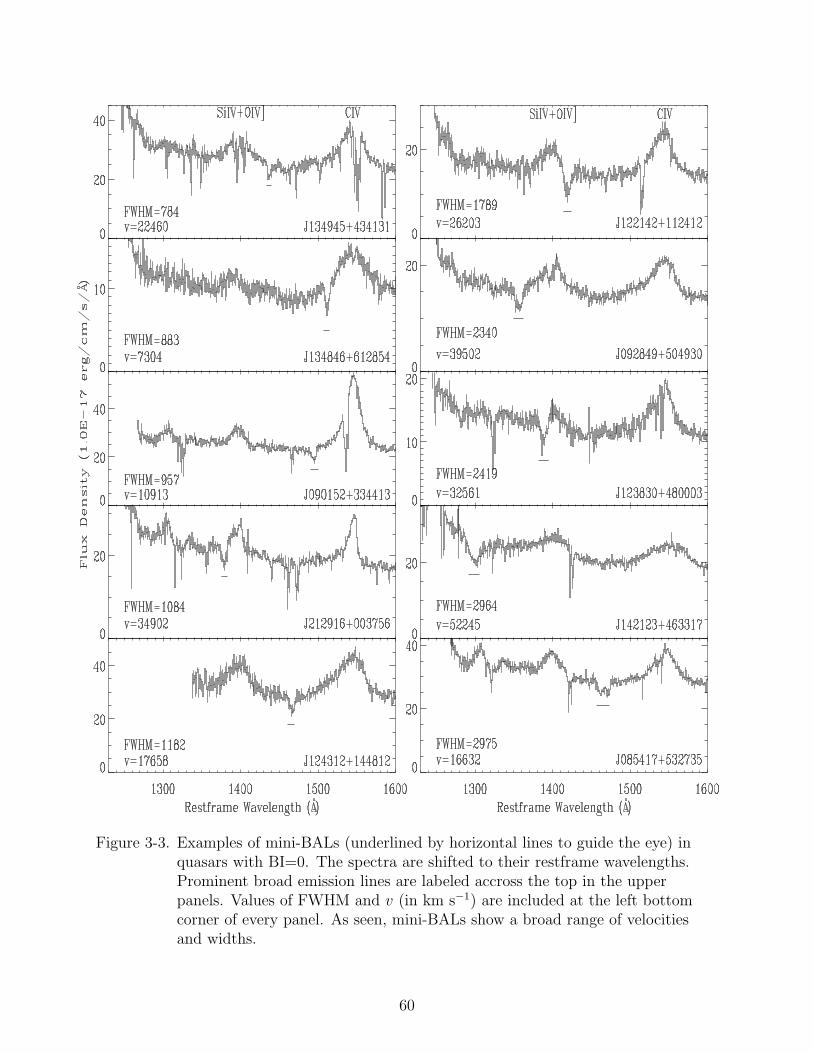
Figure 3-3. Examples of mini-BALs (underlined by horizontal lines to guide the eye) inquasars with BI=0. The spectra are shifted to their restframe wavelengths.Prominent broad emission lines are labeled accross the top in the upperpanels. Values of FWHM and v (in km s−1) are included at the left bottomcorner of every panel. As seen, mini-BALs show a broad range of velocitiesand widths.

60

Figure 3-4. Examples of mini-BALs (underlined by horizontal lines to guide the eye) inquasars with BI>0 km s−1 (left bottom corner of each plot). Values of FWHMand v (in km s−1) refer to the only mini-BAL in the spectrum or to the onewith the highest v. Note that the mini-BALs can be found by themselves or incombination with BALs, AALs, or other mini-BALs. See Figure 3-3.

61

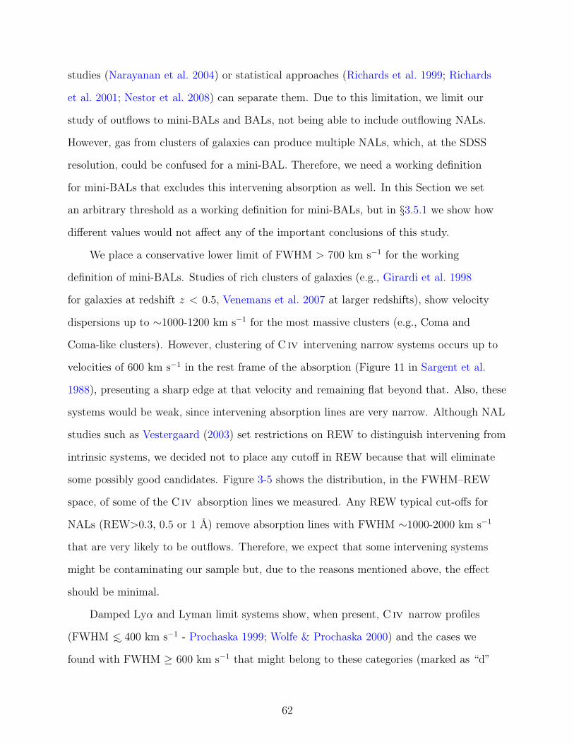
studies (Narayanan et al. 2004) or statistical approaches (Richards et al. 1999; Richards

et al. 2001; Nestor et al. 2008) can separate them. Due to this limitation, we limit our

study of outflows to mini-BALs and BALs, not being able to include outflowing NALs.

However, gas from clusters of galaxies can produce multiple NALs, which, at the SDSS

resolution, could be confused for a mini-BAL. Therefore, we need a working definition

for mini-BALs that excludes this intervening absorption as well. In this Section we set

an arbitrary threshold as a working definition for mini-BALs, but in §3.5.1 we show how

different values would not affect any of the important conclusions of this study.

We place a conservative lower limit of FWHM > 700 km s−1 for the working

definition of mini-BALs. Studies of rich clusters of galaxies (e.g., Girardi et al. 1998

for galaxies at redshift z < 0.5, Venemans et al. 2007 at larger redshifts), show velocity

dispersions up to ∼1000-1200 km s−1 for the most massive clusters (e.g., Coma and

Coma-like clusters). However, clustering of C iv intervening narrow systems occurs up to

velocities of 600 km s−1 in the rest frame of the absorption (Figure 11 in Sargent et al.

1988), presenting a sharp edge at that velocity and remaining flat beyond that. Also, these

systems would be weak, since intervening absorption lines are very narrow. Although NAL

studies such as Vestergaard (2003) set restrictions on REW to distinguish intervening from

intrinsic systems, we decided not to place any cutoff in REW because that will eliminate

some possibly good candidates. Figure 3-5 shows the distribution, in the FWHM–REW

space, of some of the C iv absorption lines we measured. Any REW typical cut-offs for

NALs (REW>0.3, 0.5 or 1 A) remove absorption lines with FWHM ∼1000-2000 km s−1

that are very likely to be outflows. Therefore, we expect that some intervening systems

might be contaminating our sample but, due to the reasons mentioned above, the effect

should be minimal.

Damped Lyα and Lyman limit systems show, when present, C iv narrow profiles

(FWHM ∼< 400 km s−1 - Prochaska 1999; Wolfe & Prochaska 2000) and the cases we

found with FWHM ≥ 600 km s−1 that might belong to these categories (marked as “d”

62

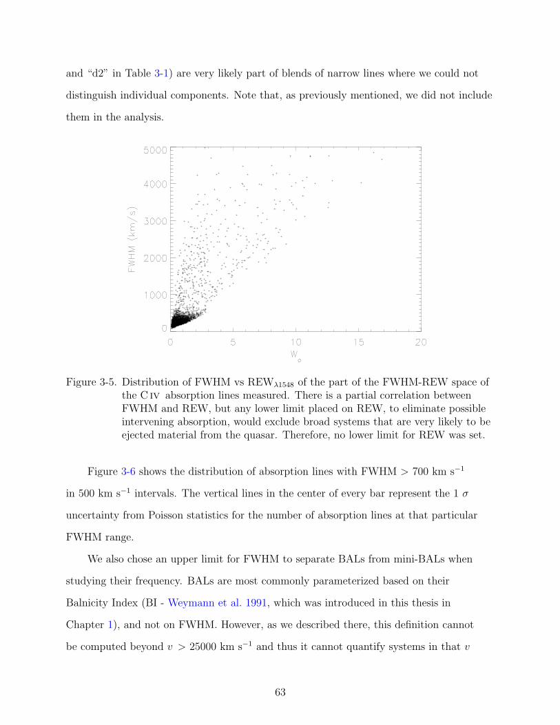
and “d2” in Table 3-1) are very likely part of blends of narrow lines where we could not

distinguish individual components. Note that, as previously mentioned, we did not include

them in the analysis.

Figure 3-5. Distribution of FWHM vs REWλ1548 of the part of the FWHM-REW space ofthe C iv absorption lines measured. There is a partial correlation betweenFWHM and REW, but any lower limit placed on REW, to eliminate possibleintervening absorption, would exclude broad systems that are very likely to beejected material from the quasar. Therefore, no lower limit for REW was set.

Figure 3-6 shows the distribution of absorption lines with FWHM > 700 km s−1

in 500 km s−1 intervals. The vertical lines in the center of every bar represent the 1 σ

uncertainty from Poisson statistics for the number of absorption lines at that particular

FWHM range.

We also chose an upper limit for FWHM to separate BALs from mini-BALs when

studying their frequency. BALs are most commonly parameterized based on their

Balnicity Index (BI - Weymann et al. 1991, which was introduced in this thesis in

Chapter 1), and not on FWHM. However, as we described there, this definition cannot

be computed beyond v > 25000 km s−1 and thus it cannot quantify systems in that v

63

Figure 3-6. Distribution in FWHM of the C iv absorption lines measured with FWHM≥700 km s−1 in intervals of 500 km s−1. Errors are shown as vertical lines in thecenter of every bar and represent the 1 σ uncertainty from Poisson statisticsfor the number of absorption lines at each particular FWHM range.

region relevant to our study. We selected an upper limit of 3000 km s−1 for the FWHM of

mini-BALs and analyzed them based on BI in the following Section.

In summary, we use a working definition for mini-BALs as absorption features with a

700 < FWHM < 3000 km s−1, and study their frequency and relationship to other classes

of absorbers in the following ection. This working definition is just a fiducial starting

point and in the following Section we also consider what effect would the selection of other

FWHM ranges have on the statistics of mini-BALs.

3.5 Statistics

In this Chapter we will use the following subsamples to maximize the number of

quasars we can use in each analysis:

• Sample A: includes every quasar we were able to measure (2174 quasars).

64

• Sample B: includes every quasar we examined, including those we could not measure(2200 quasars). This sample represents the combination of sample A and the 26BALQSOs with continua that we were not able to fit.

• Sample A2: subset of sample A that includes only quasars with zem ∼> 1.68, whichspectral coverage includes v at least up to 25000 km s−1, allowing for an accuratedefinition of BI (1983 quasars). This sample leaves out the cases with “*” in themeasurement of BI in table 3-1.

• Sample B2: subset of sample B that addresses the same issue as sample A2 (resultingin 2008 quasars). Of the 26 BALQSOs we excluded from the continua and absorptionfitting, 25 cover the region up to 25000 km s−1.

The percentages we include in this study are observed raw fractions of quasars and

not the true fractions of quasars. Our sample of quasars is not complete because we

selected only the brightest ones. Among the brightest SDSS quasars, the fractions of

quasars we present are likely close to true fractions. SDSS quasars are selected using

an i-band magnitude limit, which does not present a problem for quasars with zem ∼<3.5, where all the quasars in our sample lie. The fractions of BALQSOs would be the

most affected since the absorption alters the determination of “true” magnitudes.

Reichard et al. (2003) presented an analysis of the corrections that are applicable in

the case of obtaining the true fraction of BALQSOs. Corrections for color-dependent

selection effects as a function of redshift modified their fraction of High Ionization

BALQSOs (HiBALQSOs) from an uncorrected 14.0%±1.0% to a dust reddening corrected

13.4%±1.2% and dust reddening and extinction corrected 15.9%±1.4%. Note that their

analysis on the dust extinction is an estimation. All these corrections are likely to be

similar or smaller for the fractions of mini-BALs.

We estimate that the sample of C iv absorption has a detection threshold of

REWλ1458 ∼0.2 A for systems with FWHM ∼ 500 km s −1, REWλ1458 ∼0.3 A for

systems with FWHM ∼ 900 km s −1 and REWλ1458 ∼0.4 A for systems with FWHM

∼ 1200 km s−1, although detection threshold depends on the S/N of the spectrum in

question. Most of the candidates close to those limits are marked as questionable (“q”) in

Table 3-1.

65

3.5.1 Statistics of Mini-BALs

We have found 340 C iv mini-BALs, as defined in the previous Section, outflowing at

velocities up to 60000 km s−1, in 237 optically selected quasars with 1.6≤ zem ≤3.5 out

of the total of 2174 spectra we analyzed (sample A). We find mini-BALs in 11.4%±0.9%

quasars of the sample. No previous work has attempted to find the fraction of quasars

with mini-BALs in their spectra. Hall et al. (2002) and most recently Trump et al. (2006)

have computed AI, a more inclusive definition of the BI (see Chapter 1), over SDSS quasar

spectra, however it is an integral measurement that cannot completely characterize the

absorption.

In Figures 3-3 and 3-4 we showed that sometimes there are more than one mini-BAL

per quasar. Consequently, we present the results of (a) the number of mini-BALs per

quasar, which allows counting several mini-BALs in one quasar spectrum (Figures 3-7 and

3-8) and (b) the fraction of quasars with at least one mini-BAL at a velocity < v, which

counts only the highest-velocity mini-BAL per quasar spectrum (Figure 3-9).

Figure 3-7 shows the number of C iv mini-BALs per quasar in a particular velocity

range (per 5000 km s−1). Because not every spectrum in our sample of quasars covers

the entire velocity range (see Figure 3-1), we normalized each velocity bin by the

number of quasars available at every range. To include a quasar and a mini-BAL in

a velocity range it must cover at least 95% of that velocity bin. The three different

colors/symbols represent the number of mini-BALs per quasar in 1) all quasars from

sample A (black/squares), 2) quasars with BI < 1000 from sample B (red/diamonds), and

3) quasars with BI =0 from sample B (green/circles). The errors (vertical bars) represent

the 1 σ uncertainty from Poisson statistics for the number of systems per v interval. The

bins beyond 30000 km s−1 are in bins of width 10000 km s−1 in order to increase the

number of systems per bin and thus decrease the error bars. However, these bins still

represent the number of mini-BALs per 5000 km s−1 and therefore, are quantitatively

comparable to the others in the plot. From Figure 3-7 we can read, for example, that there

66

are 0.020±0.003 mini-BALs per quasar (2.0±0.3 per hundred of quasars) with a velocity

between 20000 and 25000 km s−1, and 0.007±0.002 mini-BALs per non-BALQSO in the

same velocity range.

Figure 3-7. Number of mini-BALs (700<FWHM<3000 km s−1) per quasar in velocityspace. The three different symbols show the mini-BALs in spectra from sampleA (black/squares), the mini-BALs in spectra with BI < 1000 from sample B(red/diamonds) and the mini-BALs in spectra with with BI = 0 from sampleB (green/circles). The horizontal width of each histogram segment indicatesthe size of the velocity bins. The vertical bars are the 1 σ uncertainties basedon counting statistics for the number of systems in that bin. The horizontallocation of each error bar marks the average velocity of all the mini-BALs inthat bin. Beyond 30000 km s−1 the bins have widths of 10000 km s−1 but stillrepresent the number of mini-BALs per 5000 km s−1.

Figure 3-8 shows the same results as in Figure 3-7 if we select other FWHM

restrictions to define what constitutes a mini-BAL. The results do not change significantly

and the shape of the distributions of the number of mini-BALs per quasar with velocity

is approximately equivalent. We selected: a) 600 < FWHM < 3000 km s−1 to show the

effects of being less cautious in the limit between intervening and outflowing absorbers, b)

900 < FWHM < 3000 km s−1 to display the effects of being more cautious in that limit,

67

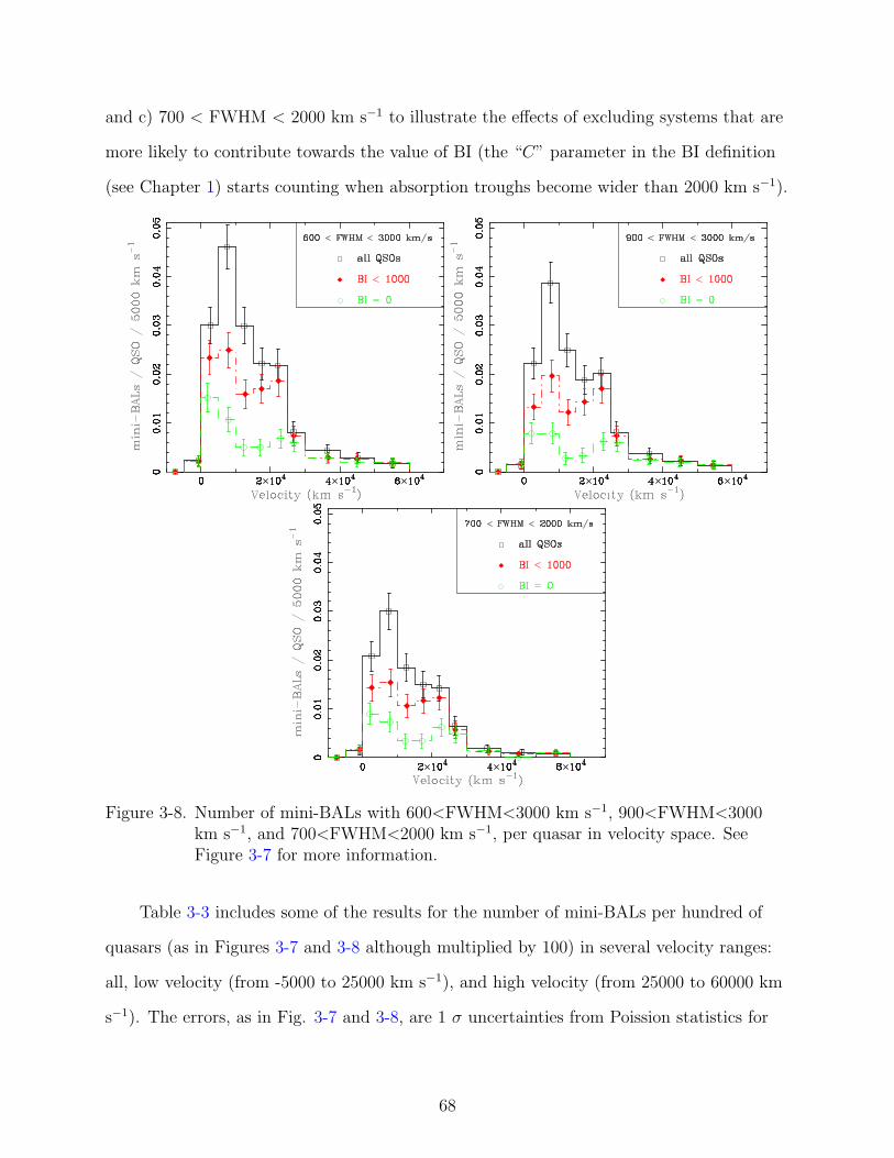
and c) 700 < FWHM < 2000 km s−1 to illustrate the effects of excluding systems that are

more likely to contribute towards the value of BI (the “C” parameter in the BI definition

(see Chapter 1) starts counting when absorption troughs become wider than 2000 km s−1).

Figure 3-8. Number of mini-BALs with 600<FWHM<3000 km s−1, 900<FWHM<3000km s−1, and 700<FWHM<2000 km s−1, per quasar in velocity space. SeeFigure 3-7 for more information.

Table 3-3 includes some of the results for the number of mini-BALs per hundred of

quasars (as in Figures 3-7 and 3-8 although multiplied by 100) in several velocity ranges:

all, low velocity (from -5000 to 25000 km s−1), and high velocity (from 25000 to 60000 km

s−1). The errors, as in Fig. 3-7 and 3-8, are 1 σ uncertainties from Poission statistics for

68

Table 3-3. Number x 100 of mini-BALs per quasar.

velocity range (km/s) sample BI 700-3000 600-3000 900-3000 700-2000-5000-60000 A (1983) all 15.5±0.8 16.4±0.9 14.2±0.8 10.9±0.7

“ A2 (1888) <1000 10.5±0.7 11.8±0.8 9.5±0.7 7.5±0.6“ A2 (1783) 0 5.4±0.5 6.4±0.6 4.8±0.5 4.0±0.5

-5000-25000 A (1983) all 12.9±0.8 13.6±0.8 11.8±0.7 9.3±0.7” A2 (1888) <1000 8.2±0.7 9.4±0.7 7.4±0.6 6.2±0.6” A2 (1783) 0 3.4±0.4 4.2±0.5 2.8±0.4 2.9±0.4

25000-60000 A (1983) all 2.5±0.4 2.5±0.4 2.2±0.3 1.4±0.3” A2 (1888) <1000 2.1±0.3 2.2±0.4 2.0±0.3 1.2±0.3” A2 (1783) 0 1.8±0.3 1.9±0.3 1.8±0.3 1.0±0.2

the number of systems in that v interval. For example, Table 3-3 includes that there are

15.5±0.8 mini-BALs at any v per hundred sample quasars.

Figure 3-9 shows the fraction of quasars with at least one mini-BAL. It includes a)

the fraction of quasars that have at least one mini-BAL at velocity “< v” (upper plots)

and b) the fraction of quasars with at least one mini-BAL outflowing at a velocity from

25000 km s−1 to v (lower plots). In these cases we have used only the basic working

definition for mini-BALs (700 < FWHM < 3000 km s−1). The color coding represents

the same three samples of all quasars, BI < 1000, and BI = 0, as in Figure 3-7. Dotted

lines represent the errors. Only quasars that cover up to 95% of each velocity range are

included. These fractions of quasars are not monotonically increasing functions because

the number of quasars in the samples diminishes after ∼17000 km s−1.

Table 3-4 summarizes some of the results of the fraction of quasars with mini-BALs

for the basic working definition (700 < FWHM < 3000 km s−1) at several velocity

ranges from Figure 3-9. For example, we find that there are 11.4%±0.9% quasars with a

mini-BAL at any v. If we only select quasars with BI=0, there are 5.1% of them that show

a mini-BAL at any velocity. As expected, the results are smaller than in Table 3-3 because

we are counting only one mini-BAL per quasar spectrum. Doing so avoids the problem of

double-counting and deblending stated in §3.3.

Overall, Figures 3-7–3-9 and accompanying Tables 3-3–3-4 show that there is a

significant number of mini-BALs in our sample of quasars, independent of the FWHM

69

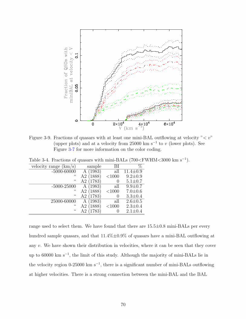
Figure 3-9. Fractions of quasars with at least one mini-BAL outflowing at velocity ”< v”(upper plots) and at a velocity from 25000 km s−1 to v (lower plots). SeeFigure 3-7 for more information on the color coding.

Table 3-4. Fractions of quasars with mini-BALs (700<FWHM<3000 km s−1).

velocity range (km/s) sample BI %-5000-60000 A (1983) all 11.4±0.9

“ A2 (1888) <1000 9.2±0.9“ A2 (1783) 0 5.1±0.7

-5000-25000 A (1983) all 9.9±0.7“ A2 (1888) <1000 7.0±0.6“ A2 (1783) 0 3.3±0.4

25000-60000 A (1983) all 2.6±0.5“ A2 (1888) <1000 2.3±0.4“ A2 (1783) 0 2.1±0.4

range used to select them. We have found that there are 15.5±0.8 mini-BALs per every

hundred sample quasars, and that 11.4%±0.9% of quasars have a mini-BAL outflowing at

any v. We have shown their distribution in velocities, where it can be seen that they cover

up to 60000 km s−1, the limit of this study. Although the majority of mini-BALs lie in

the velocity region 0-25000 km s−1, there is a significant number of mini-BALs outflowing

at higher velocities. There is a strong connection between the mini-BAL and the BAL

70

phenomenon and we will discuss the percentages of mini-BALs in quasars with different

values of BI in §3.5.2.

3.5.2 Relation between Mini-BALs and BALs

In this section we explore how frequently mini-BALs appear in BALQSOs versus

in non-BALQSOs. BALQSOs are defined as those with BI>0 and non-BALQSOs as

those with BI = 0 (see Chapter 1). Our study finds an observed fraction of 10.7%±0.7%

BALQSOs out of the quasars in sample B, whereas 5.7%±0.5% have BI > 1000, and

4.2%±0.4% have BI > 2000. We estimate that all of the 26 unanalyzed BALQSOs have BI

> 2000. Previous studies also based on SDSS samples and BI measurements find similar

percentages. Reichard et al. (2003) found an observed fraction of 14.0%±1.0% BALQSOs

out of a sample of 3814 quasars with 1.7 ≤ zem ≤ 4.2. Trump et al. (2006), improving the

continuum fitting technique and enlarging the sample to 16883 quasars with 1.7 ≤ zem ≤4.38, reported a BALQSO observed fraction of 10.4%±0.2%. Besides the differences

in redshift coverage with our sample, both works rely on the use of templates to place

the continuum, while we fit pseudo-continua with a spline function for the underlying

continuum and Gaussians for the broad emission lines. Nonetheless, the value obtained by

Trump et al. (2006) and ours coincide within the error.

As Figures 3-3, 3-4 and 3-7-3-9 illustrate, mini-BALs are present in both BALQSOs

and non-BALQSOs. In Figure 3-7 we showed the number of mini-BALs in all quasars,

quasars with BI<1000 and quasars with BI=0. Because we find more than one mini-BAL

in some quasar spectra we also present separately the fraction of quasars with, at least, a

mini-BAL at velocity < v.

Figure 3-10 summarizes some of our results on the fraction of quasars with at least

one mini-BAL at a velocity < v from Figure 3-9 and Table 3-9, and compares them to

the fraction of BALQSOs with different values of BI. Figure 3-10, in the same fashion

as Figure 3-9, includes the fraction of quasars with three different cutoffs of BI: any BI,

BI<1000 and BI=0. All of the percentages of fractions of quasars with mini-BALs are

71

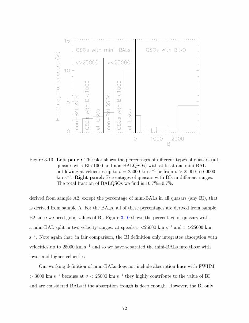
Figure 3-10. Left panel: The plot shows the percentages of different types of quasars (all,quasars with BI<1000 and non-BALQSOs) with at least one mini-BALoutflowing at velocities up to v = 25000 km s−1 or from v > 25000 to 60000km s−1. Right panel: Percentages of quasars with BIs in different ranges.The total fraction of BALQSOs we find is 10.7%±0.7%.

derived from sample A2, except the percentage of mini-BALs in all quasars (any BI), that

is derived from sample A. For the BALs, all of these percentages are derived from sample

B2 since we need good values of BI. Figure 3-10 shows the percentage of quasars with

a mini-BAL split in two velocity ranges: at speeds v <25000 km s−1 and v >25000 km

s−1. Note again that, in fair comparison, the BI definition only integrates absorption with

velocities up to 25000 km s−1 and so we have separated the mini-BALs into those with

lower and higher velocities.

Our working definition of mini-BALs does not include absorption lines with FWHM

> 3000 km s−1 because at v < 25000 km s−1 they highly contribute to the value of BI

and are considered BALs if the absorption trough is deep enough. However, the BI only

72

Figure 3-11. Percentages of absorption lines with FWHM>3000 km s−1 per quasar per5000 km s−1 bin in velocity space. See Fig. 3-7 for information on what thedifferent symbols represent. The arrows indicate that these values are lowerlimits since we are not including the 26 BALQSOs that we did not analyze.

covers up to 25000 km s−1 and thus absorption lines with FWHM > 3000 km s−1 at

higher velocities belong to an ‘absorption limbo’: they do not count towards BI and are

not included in the mini-BAL working definition. Figure 3-11 shows the distribution with

velocity of absorption lines with FWHM > 3000 km s−1 per quasar. There are 0.8±0.2%

absorption lines with FWHM > 3000 km s−1 per non-BALQSO outflowing at v > 25000

km s−1. We use sample A for the ‘all’ cases and sample A2 for the cases with BI<1000

and BI=0; note that the number of absorption lines in all quasars do not include the

non-measured BALQSOs, which is symbolized by the arrows in that result.

Mini-BALs are not just part of BAL absorption troughs, and they represent a part

of the FWHM–velocity space of quasar outflows that has barely been studied before.

There are 0.155±0.008 mini-BALs at any velocity per quasar and 0.054±0.005 mini-BALs

outflowing at any velocity per nonBALQSO. We find that the difference between the

number of mini-BALs per quasar in all quasars versus in non-BALQSOs is larger at

73

lower velocities (0.129±0.008 in all quasars versus 0.034±0.004 in non-BALQSOs), while

mini-BALs with v > 25000 km s−1 are more common in non-BALQSOs (0.025%±0.004%

in all quasars versus 0.018%±0.003% in non-BALQSOs). This trend suggests that the

presence of absorption at low velocities tends to not be accompanied by high-velocity

absorption; in other words, that the probability of finding a mini-BAL at v > 25000 km

s−1 is independent of the presence of BALs at lower velocities. However, we must note

that we might be underestimating the presence of C iv at high velocities in spectra where

C iv is also present at low velocities because of the possible confusion with Si iv. Also,

because we find more than one mini-BAL in some quasar spectra, we have presented

separately the fraction of quasars with, at least, a mini-BAL at velocity < v. We find

that 11.4%±0.9% quasars have at least one mini-BAL at any velocity, noting that almost

half of them, 5.1%±0.7%, are non-BALQSOs. The majority of quasars with a mini-BAL

outflowing at v ≥ 25000 km s−1 are non-BALQSOs (2.1%±0.4% in non-BALQSOs versus

2.6±0.5% in all quasars).

3.5.3 Relation between Mini-BALs and AALs

In this section we explore whether there is a connection between the presence of

mini-BALs and associated absorption lines (AALs - see Chapter 1). Figures 3-3 and 3-4

show several examples of quasar spectra where both mini-BALs and AALs are present.

We now specify what we would consider AALQSOs. First of all, we exclude

BALQSOs from consideration. The non-BALQSOs (1783 quasars with BI = 0) are

selected from sample A2 because an accurate limit on BI is necessary. Associated

absorption systems are usually defined as those that have velocities up to 5000 km s−1

relative to the systemic redshift (Foltz et al. 1986); we use this value as an upper limit

for their velocity. Because the statistical error in the determination of the zero velocity is

based on the SDSS systemic redshift, we include systems down to -1000 km s−1. Following

Vestergaard (2003), Nestor et al. (2008) and Fox et al. (2008), we exclude weak AALs

74

because they are more likely to be intervening. We use a cutoff of REWλ1548 ≥ 0.3.

Finally, we did not restrict the value of FWHM.

Of the quasars in sample A2 that are non-BALQSOs (1783), 26.2%±1.2% are

AALQSOs set by the above criteria: non-BALQSO with at least one absorption line at

-1000< v <5000 km s−1 and REWλ1548 ≥0.3. Note that in Nestor et al. (2008) we reported

a fraction of 25% AALQSOs, but in Nestor et al. (2008) we included only absorption with

FWHM < 600 km s−1, and in the current analysis we have not set any restrictions in

FWHM. Vestergaard (2003) reported a fraction of 27% AALQSOs, but their restrictions

in v and REW were slightly different.1 Vestergaard (2003) also includes the fractions of

AALQSOs with other REW constraints (e.g., 25% with REW ≥ 1 A).

Nestor et al. (2008) carried out a statistical analysis which found an excess (larger

than 60%) of, very likely, outflowing narrow absorption, among associated absorption,

with velocities between 1800 and 4400 km s−1 blueshifted relative to the quasar systemic

velocity. We use this range as well since it seems to include systems that are more likely to

be outflowing AALs than the velocity cutoff mentioned above.

Figure 3-12 shows the normalized distribution in velocity of the number of mini-BALs

with v > 5000 km s−1 in AALQSOs and non-AALQSOs in different velocity bins, in the

same fashion as explained for Figure 3-7 in §3.5.1. It includes the results for both velocity

cutoffs to select AALQSOs: -1000 < v < 5000 km s−1 and 1800 < v < 4400 km s−1.

The lack of mini-BALs in both AALQSOs and non-AALQSOs with v < 5000 km s−1

is a consequence of our decision to exclude those cases in this study so they cannot be

double-counted as mini-BAL and AAL. However, the absence of mini-BALs with v >

40000 km s−1 in AALQSOs is possibly real.

In Table 3-5 we include the number of AALQSOs and non-AALQSOs based on the

two sets of constraints described above and the number of them that includes a mini-BAL

1 |v| ≤ 5000 km s−1 and total REW of the C iv doublet ≥ 0.5 A.

75

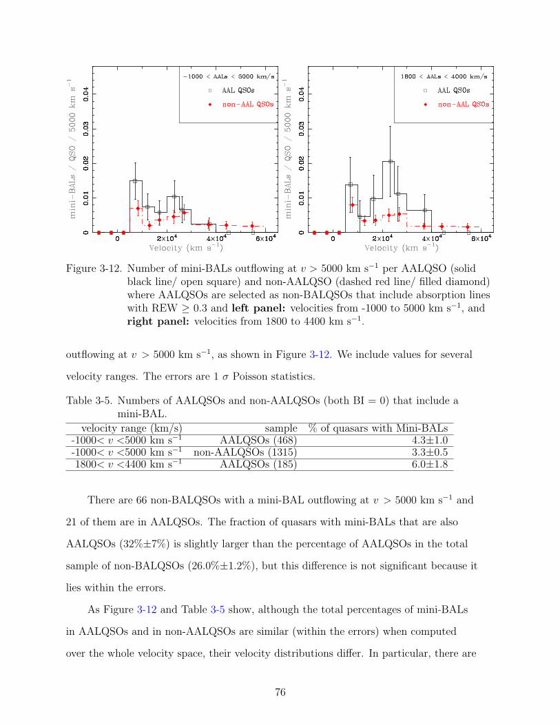
Figure 3-12. Number of mini-BALs outflowing at v > 5000 km s−1 per AALQSO (solidblack line/ open square) and non-AALQSO (dashed red line/ filled diamond)where AALQSOs are selected as non-BALQSOs that include absorption lineswith REW ≥ 0.3 and left panel: velocities from -1000 to 5000 km s−1, andright panel: velocities from 1800 to 4400 km s−1.

outflowing at v > 5000 km s−1, as shown in Figure 3-12. We include values for several

velocity ranges. The errors are 1 σ Poisson statistics.

Table 3-5. Numbers of AALQSOs and non-AALQSOs (both BI = 0) that include amini-BAL.

velocity range (km/s) sample % of quasars with Mini-BALs-1000< v <5000 km s−1 AALQSOs (468) 4.3±1.0-1000< v <5000 km s−1 non-AALQSOs (1315) 3.3±0.51800< v <4400 km s−1 AALQSOs (185) 6.0±1.8

There are 66 non-BALQSOs with a mini-BAL outflowing at v > 5000 km s−1 and

21 of them are in AALQSOs. The fraction of quasars with mini-BALs that are also

AALQSOs (32%±7%) is slightly larger than the percentage of AALQSOs in the total

sample of non-BALQSOs (26.0%±1.2%), but this difference is not significant because it

lies within the errors.

As Figure 3-12 and Table 3-5 show, although the total percentages of mini-BALs

in AALQSOs and in non-AALQSOs are similar (within the errors) when computed

over the whole velocity space, their velocity distributions differ. In particular, there are

76

not mini-BALs in AALQSOs outflowing at velocities larger than 40000 km s−1. If we

consider only AALs in the velocity range 1800 < v < 4400 km s−1 we find a slightly larger

percentage of AALQSOs with mini-BALs.

3.5.4 Relation between C iv Mini-BALs and Mg ii Absorption

We visually inspected every quasar with C iv absorption broader than 500 km s−1

and every quasar with associated absorption to search for Mg ii λλ2796,2804 absorption

at similar velocities. The samples searched were construed to have zem < 2.25 so Mg ii

lies within the spectral wavelength range and 1) C iv absorption with FWHM > 500

km s−1 (271 quasars, subset of sample B) and/or 2) associated absorption as defined in

section §3.5.3 (343 quasars, subset of sample A2). Also, out of sample of 271 quasars that

presented absorption with FWHM > 500 km s−1, we created another subset that includes

only quasars with mini-BALs (175 quasars). We did not perform continuum fitting across

the Mg ii wavelengths. Assessing the presence of Mg ii absorption at the same velocities

as C iv became a difficult task due to the presence of Fe ii lines in the shortward of the

Mg ii emission line, which makes it difficult to decide whether there is absorption or there

are two emission lines side by side, producing a false absorption effect. Note that we are

not including either the “d” or “d2” in Table 3-1 since they are Damped Lyα systems or

likely to be them, respectively.

Figure 3-13 shows some examples of cases where we find Mg ii absorption at the

same v as C iv. All of the Mg ii systems we find in this search are either 1) BALs, where

the Mg ii was broad but narrower and weaker than C iv, or 2) associated lines, where

in most cases the Mg ii absorption appeared strong. In the cases where a C iv BAL is

accompanied by Mg ii, this absorber was sometimes outflowing at lower velocities than the

C iv absorber, which has been previously reported (i.e., Weymann et al. 1991; Voit et al.

1993).

We do not find any Mg ii absorption accompanying C iv mini-BALs in the 175 quasar

spectra analyzed. Since we have not normalized the continuum around the Mg ii emission

77

Figure 3-13. Examples of Mg ii (lower panels) outflowing with C iv (upper panels).Vertical dashed lines are situated approximately where the left side of theMg ii doublet would fall to guide the eye. Left panels: C iv BAL with itscorresponding Mg ii mini-BAL. Because Mg ii absorption in outflows seem tobe weaker than their relative C iv ones, only in strong broad BALs we areable to detect obvious Mg ii mini-BALs in the same outflow. Right panels:3 different systems (from left to right): a) a C iv mini-BAL with nocorrespondent Mg ii b) a very likely Damped Lα system with strong MgIIabsorption (among other low ionization lines) and weak C iv, and c) strongassociated C iv absorption with very weak Mg ii.

78

line region, we cannot completely discard the existence of Mg ii absorption together with

C iv mini-BALs. However, if present, Mg ii would be very weak. Whenever strong C iv

BALs are accompanied by Mg ii, the latter is always weaker (see Figure 3-13), which

is also reported in Voit et al. (1993). This tendency suggests that, if present, the Mg ii

absorption at the same v as C iv mini-BALs might be even weaker and difficult to detect

without a proper continuum fitting.

We find that 9.0%±1.5% of C iv AALs with zem <2.25 also present Mg ii (37 out of

410). We obtained approximately the same percentage (9%±2%, 15 out of 160) selecting

only those quasars with 1800< v <4400 km s−1 (see §3.5.3). C iv BALQSOs included

Mg ii absorption in their spectra in 7.0%±1.9% of cases (13 out of 187). As mentioned

above, the estimated fraction of quasars with C iv mini-BALs that present Mg ii is 0% (0

out of 175).

3.5.5 Relation between C iv Mini-BALs and Radio Properties

In this section we study the radio properties of quasars with absorption broader

than 500 km s−1. Originally BALQSOs were thought to be radio quiet objects (Stocke

et al. 1992 - hereafter S92; de Kool 1993). However, since then, many cases of radio-loud

BALQSOs have been found (e.g., Brotherton et al. 1998; Becker et al. 2000; Menou et al.

2001; Brotherton et al. 2005; McGreer et al. 2006). In order to investigate possible trends

between quasars with outflows and their radio properties we have cross-correlated our

sample of quasars with the Faint Images of the Radio Sky at Twenty cm survey (FIRST;

Becker et al. 1995). Out of the initial 2200 quasars (sample B), 259 of these are FIRST

detected (FIRST detection threshold is 1mJy), having a matching radio source within 10”,

1758 were non-detected, while the remainder were not covered by FIRST. All of the 2017

quasar detections except for 14 lie within 2” of the SDSS position, and whenever there

were several matches for one source, we selected the closest one to the SDSS coordinates.

79

In order to define whether the FIRST detected quasars are radio-loud or radio-quiet,

we use the parameter R∗ (Sramek & Weedman 1980) that is a relative measurement of the

radio flux at 5 Ghz versus the optical flux at 2500 A:

log R∗ = log f(5GHz)− log f(2500A). (3–1)

The radio flux at 5 GHz can be defined in terms of the FIRST peak flux Sν (in

mJy/beam), the frequency ν (1.4 GHz), the radio spectral slope αrad, which we assumed

to be 0.3 for every quasar following Sramek & Weedman (1980), and the SDSS systemic

redshift zem. We use the formula introduced in Sramek & Weedman (1980):

log f(5GHz) = −29.0 + log(Sν) + αrad log[5/ν]− (1 + αrad) log(1 + zem). (3–2)

In order to define the optical flux at 2500 A, we do not consider appropriate the use

of the filter-B magnitude (centered at 4361 A) for our sample, since the majority of the

quasars in our sample have a redshift zem ∼ 2. This redshift places the C iv emission line

at ∼ 4650 A, contaminating the B-magnitude value with absorption and emission. Instead

we derived log f(2500 A) from the SDSS r-magnitudes (centered at 6122 A):

log f(2500A) = −22.83− 0.4rc, (3–3)

where rc is the r SDSS magnitude corrected from Galactic extinction2 , and a spectral

index, αopt, of -1 (fν ∝ ν−αopt) is used.

Stocke et al. (1992) divided radio-loud and radio-quiet QSOs at zem ≈ 2 as having

log R∗ larger or smaller than unity, respectively, and we use the same criteria. Figure 3-14

shows the distribution of radio sources among the absorbers with FWHM > 500 km s−1

2 using extinctions from http://irsa.ipac.caltech.edu/applications/DUST.

80

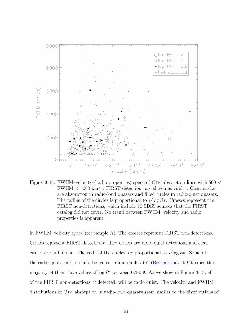
Figure 3-14. FWHM–velocity–(radio properties) space of C iv absorption lines with 500 <FWHM < 5000 km/s. FIRST detections are shown as circles. Clear circlesare absorption in radio-loud quasars and filled circles in radio-quiet quasars.The radius of the circles is proportional to

√log R∗. Crosses represent the

FIRST non-detections, which include 16 SDSS sources that the FIRSTcatalog did not cover. No trend between FWHM, velocity and radioproperties is apparent.

in FWHM–velocity space (for sample A). The crosses represent FIRST non-detections.

Circles represent FIRST detections: filled circles are radio-quiet detections and clear

circles are radio-loud. The radii of the circles are proportional to√

log R∗. Some of

the radio-quiet sources could be called “radio-moderate” (Becker et al. 1997), since the

majority of them have values of log R∗ between 0.3-0.9. As we show in Figure 3-15, all

of the FIRST non-detections, if detected, will be radio quiet. The velocity and FWHM

distributions of C iv absorption in radio-loud quasars seem similar to the distributions of

81

C iv absorption in radio-quiet sources, and we do not find any significant trend, with the

exception of finding that the strongest radio-loud sources in our sample (log R∗ ≥ 2) are

all non-BALQSOs with associated and low velocity systems (within v < 7000 km s−1 from

the systemic velocity).

Figure 3-15 shows radio-loudness (log R∗) versus quasar Balnicity Index for the

quasars in the same sample as those in Figure 3-14. Symbols have same meaning as in

Figure 3-14 except for the arrows that represent upper limits for sources that FIRST

covered but were not detected (the top of the arrow is placed at the upper limit of the

log R∗ value, derived from a Sν =0.9 mJy/beam, a little bit below the FIRST detection

limit of 1 mJy). Inspection of Figure 3-15 suggests gaps of radio loudness for certain

Balnicity Indexes: none of the quasars with BI between 200 and 1400 are radio-loud (0 out

of 58), while 12% (6 out of 50) of the quasars with 0 < BI < 200 and 12% (7 out of 59) of

the quasars with 1400 < BI < 4200 are. Another gap appears beyond a BI of 4200 (0 out

of 16).

We find that out of the 2017 quasars in this study covered by FIRST, 8.9%±0.7%

are radio-loud. Of the quasars with absorption lines with FWHM ≥ 500 km s−1 in

sample B, there are 7.5%±1.5% radio-loud sources. Of these ones, whereas 8%±2%

of the non-BALQSOs are radio-loud, 6.8%±1.8 of BALQSOs are radio-loud. In the

case of quasars with mini-BALs, we also find that 7.4%±1.8% of them are radio-loud,

approximately the same percentage as those from BALQSOs and quasars with mini-BALs

combined (7.1%±1.5%).

3.6 Discussion

We have performed the first complete inventory of all C iv absorption lines in a

sample of 2200 bright SDSS quasars at redshifts 1.6 ≤ zem ≤ 3.5. Our main goals are to

1) examine the velocity distribution of the absorption lines relative to the quasar systemic

redshift (see also Nestor et al. 2008), and 2) identify individual outflow lines and candidate

outflow lines for statistical analysis and follow-up studies. We are particularly interested

82

Figure 3-15. Radio loudness versus Balnicity Index of the quasars with absorption inFigure 3-14. FIRST detections are shown as circles. Clear circles representabsorption in radio-loud quasars and filled circles in radio-quiet quasars. Theradius of the circles is proportional to

√log R∗. Arrows represent the FIRST

non-detections where the top of the arrow is placed at the upper limit(Sν =0.9 mJy/beam). Crosses at the bottom of the Figure are the 16 SDSSsources that the FIRST catalog did not cover.

in outflow features that are underrepresented in previous work, namely, mini-BALs and

high velocity systems with v > 25000 km s−1. All this information can be supplemented

by previous results based on integrated absorption measurements, such as BI and AI.

Our quasar sample selects the brightest objects, and therefore it is not complete.

We have selected several subsamples to maximize the statistical results of the different

studies we have carried out (see §3.5). The results we derive are observed raw fractions

of quasars and not the true fractions of quasars, because we have not performed dust

reddening or extinction corrections. Reichard et al. (2003) analyzes these effects for a

sample of BALQSOs, which are expected to be the most affected by absorption extinction.

83

Their corrections modify the raw fraction of BALQSOs by less than 2%. Note that for

SDSS quasars with zem ∼< 3.5, as every quasar in our sample, these fractions do not need

to be corrected by the absorption trough since SDSS quasars are selected using the i-band

magnitude limit.

We present, for the first time, the number of mini-BALs expected per quasar

spectrum. We have attempted to exclude intervening absorption that, at the SDSS

resolution, could appear similar to mini-BALs. To do so, we introduce a working definition

that selects mini-BALs as absorption lines with FWHMs larger than 700 km s−1. By using

a FWHM cutoff of 700 - 3000 km s−1, we find that there are 15.5±0.8 mini-BALs per

hundred quasars. We have also reported the frequency of absorption with other possible

FWHM selections, which resulted in similar results. We have presented their distribution

in velocity (Fig. 3-7 and 3-8) in all quasars, non-BALQSOs and quasars with BI < 1000

km s−1. Because some quasar spectra include more than one mini-BAL, and in order to

avoid double-counting, we also have computed the fraction of quasars with at least one

mini-BAL at any velocity, finding that 11.4%±0.9% of quasars have at least one mini-BAL

at any velocity.

The mini-BAL phenomenon is strongly related to BALQSOs. Approximately 7% of

the quasars in sample A2 are BALQSOs that also include a mini-BAL at v < 25000 km

s−1. Our quasar sample includes 10.7%±0.7% BALQSOs, which are defined to have BI >

0. Other studies based also on SDSS quasar samples find similar percentages: Trump et al.

(2006) finds 10.4%±0.2% BALQSOs, and Reichard et al. (2003) reports a raw fraction of

14.0%±1.0%. Previous studies in other samples of optically selected quasars also reported

fractions similar to these values; i.e., Hewett & Foltz (2003) reported a non-corrected

fraction of 15%±3% BALQSOs in the Large Bright Quasar Survey (LBQS), however this

result is not directly comparable to ours since they take into account, not only BI, but

also the probability of a quasar of being a BALQSO (P ). Using their number of BALQSOs

within the range 1.5 ≤ zem ≤ 3.0 and magnitude interval 16.50-18.85, they obtain a

84

fraction of 10.7%±1.7%. From the perspective of computing the total fraction of quasars

with any kind of outflows, the percentage of BALQSOs with mini-BALs is included in the

above fraction of BALQSOs and therefore we will not include it hereafter.

Mini-BALs are also part of two regions of the outflow parameter space that have

been sparsely surveyed before: non-BALQSOs and high velocity systems. We have found

that mini-BALs are present, at any velocity, in 5.1%±0.7% of non-BALQSOs. If we select

only those that are found at v < 25000 km s−1, we still find mini-BALs in 3.4%±0.4% of

non-BALQSOs. At larger velocities (25000 km s−1 < v ∼< 0.2c), 2.5%±0.4% of the quasars

of any type, not only BALQSOs, show at least one mini-BAL. Most of the mini-BALs

at these velocities appear in non-BALQSOs. The study of these high velocity outflows is

necessary because it may help to constrain the acceleration mechanisms that have been

proposed to drive them outside of the SMBH environment.

Mini-BALs are not the only type of absorption barely studied in previous surveys.

We also have found broad absorption that has not been included in any of the previous

categories. Traditionally BALQSO definitions based on BI measured over the C iv

short-ward wavelength range have been limited to a velocity of 25000 km s−1 in order

to avoid confusing it with Si iv absorption, and no other comprehensive studies have

been carried out beyond this velocity. Consequently, we also investigated the frequency

of absorption lines with FWHM > 3000 km s−1. Figure 3-11 shows the distribution in

velocity of these absorption lines, which at v > 25000 km s−1 are present in 0.8%±0.2% of

non-BALQSOs. Mini-BALs are therefore more common at very high velocities than wider

absorption lines, but both mini-BALs and broader absorption seem to reach the maximum

terminal velocities of this study (∼ 0.2c). Excluding those that include also mini-BALs

in their spectra, there are 0.4%±0.2% non-BALQSOs with these broad absorbers, and

together with the fraction of mini-BALs, we obtain a fraction of ∼ 5.5% non-BALQSOs

with outflows. This fraction can be added to the fraction of BALQSOs resulting in a

85

fraction of ∼ 16% quasars with mini-BALs and broad absorption, which are presumably

quasar outflows.

The frequency of AALQSOs in our sample is 26.2%±1.2% of the non-BALQSOs.

In Nestor et al. (2008) we reported the AALQSO frequency when including only the

absorption lines with FWHM < 600 km s−1 (25%). These fractions are comparable to

results of other quasar studies at similar redshifts (Vestergaard 2003 - 27%±5%, Misawa

et al. 2007a - 23%), and even with quasars at lower redshifts (Ganguly et al. 2001, found

25%±6% from 59 quasars at zem < 1), although these comparisons between different

samples are non-trivial because of the heterogenous definitions of what AALs are. Our

analysis of AALs was derived from the sample of non-BALQSOs, and is thus independent

of the frequency of BALs. We have not found a solid relationship between the presence of

mini-BALs in either AALQSOs or in non-AALQSOs. Mini-BALs outflowing at v > 5000

km s−1 appear in 5% of AALQSOs, whereas they are present in 3% of non-AALQSOs.

However, the distribution in velocity of the mini-BALs in AALQSOs seems to be more

concentrated than in non-AALQSOs, as we do not find mini-BALs with v > 40000 km

s−1 in AALQSOs, although mini-BALs occur at those velocities in non-AALQSOs. The

fraction of quasars with AALs that have not been included in the previous fractions (i.e.,

those which not include a mini-BAL or BAL at any velocity) is 25%. Although it is known

that most AALs are part of the host galaxy-AGN environment, it is unclear whether

AALs are ejected material or already part of the host galaxy. In Nestor et al. (2008) we

reported an excess of narrow absorption lines blue-shifted with respect to the quasar

systemic velocity, and therefore likely to be intrinsic to the quasar outflow phenomenon.

Wise et al. (2004) reported that ≥ 20% of a sample of 19 C iv AALs are intrinsic to

the quasar central engine based on time-variability studies and Misawa et al. (2007a)

obtained a larger fraction (∼ 33%) based on partial coverage of a sample of 37 quasars.

Assuming that all the AALQSOs in our study include outflowing AALs, we can add it to

the outflows tally, obtaining ∼ 41% quasars with outflows.

86

Besides AALs, several studies have found that higher velocity NALs might also be

part of outflows. Richards et al. (1999) and Richards et al. (2001) found large fractions

(36%) of non-intervening narrow absorption lines at v ∼ 5000 - 55000 km s−1 based

on correlations with quasar intrinsic radio properties of their sample. By studying

high-velocity NALs on a one-on-one basis, Misawa et al. (2007a) reported that 10-17%

of non-associated C iv NAL systems with v ∼ 5000 - 70000 km s−1 show partial coverage,

characteristic of non-intervening absorption. Note that both percentages are not in conflict

since partial coverage is a signature but not a requirement of quasar outflowing nature,

and therefore the result reported by Misawa et al. (2007a) might be included in the

Richards et al. (1999) percentage. As noticed in Ganguly & Brotherton (2008), this is not

the fraction of quasars hosting these outflows but the fraction of intrinsic systems in the

sample. The total fraction of quasars with outflows, obtained from adding the percentages

above, is 41-77%, which we express as a range because of the possibility that quasars in

the study reported in Richards et al. (1999) show more than one C iv system and also

the possibility of overlapping with some of other the classes we described above. Ganguly

& Brotherton (2008) presented a review of recent surveys of quasar absorption lines, and

reached a fraction of 57%-80% quasars with outflows. They used a corrected fraction of

quasars with BALs (Hewett & Foltz 2003) and did not consider a possible total overlap

between AALQSOs and quasars with mini-BALs or high velocity absorbers.

Our analysis includes also the study of low ionization lines at the same zabs as the

C iv absorption. Weymann et al. (1991) observed that ∼10% of C iv BALQSOs are

accompanied by “obvious Mg ii and/or Al iii absorption trough”, which were determined

by visual inspection of the spectra. Using an adapted version of BI for the Mg ii emission

line region, Trump et al. (2006) reported that 0.55%±0.04% of the SDSS quasars at

0.5≤ zem ≤2.15 show Mg ii absorption. Selecting only those classified as C iv BALQSOs

where Mg ii is within the spectral coverage, they obtain that 7.4%±0.5% of BALQSOs

present Mg ii absorption. We have studied the presence of Mg ii by visual inspection

87

of the spectra of subsamples of quasars with zem ≤2.25 and with 1) C iv absorption

broader than 500 km s−1 (which includes BALQSOs) and 2) AALs. We report that

7.0%±1.9% of the C iv BALQSOs in our sample B are accompanied by Mg ii absorption

and 9.0%±1.5% of the C iv AALQSOs include Mg ii in their spectra at approximately

the same velocity as the C iv AAL. However, we do not find any case of C iv mini-BALs

where there is a positive detection of Mg ii at similar velocities. Note, however, that

because we have not fit the continuum and there are Fe ii emission lines in the short-ward

of the Mg ii emission line, it is not possible to conclude that there is a lack of Mg ii

accompanying the C iv mini-BALs. Nonetheless, if present, this absorption would be very

weak. We were expecting the Mg ii absorption to be weaker than the C iv mini-BALs

since previous studies show that, in C iv BALQSOs, Mg ii appears to be weaker than the

C iv absorption (Voit et al. 1993).

We also study the radio properties of all the quasars in our sample (sample B),

and find that 8.9%±0.7% of the ones detected by FIRST are radio-loud, as defined to

have log R∗ ≥ 1. Quasars with mini-BALs and BALs show a slightly smaller fraction

of radio-loud sources (7.4%±1.8% and 6.8%±1.8%, respectively), which may not

be a significant difference. Whereas we do not find any correlations between quasar

radio-loudness and the FWHM or v of the absorption, or with the BI of the quasars,

we report that the strongest radio-sources in our sample (log R∗ > 2) are all quasars

with associated absorption or low v absorption (v < 7000 km s−1). This result agrees

with Richards et al. (2001), where it was reported that the population of quasars with

AALs tend to show larger values of RV (defined similarly to R∗ although using 20 cm

measurements instead of 5 GHz).

In summary, with the goal of computing the fraction of quasars with outflows, we

have reached a total fraction of ∼ 16% quasars with outflows with FWHM > 700 km s−1,

which is the result of adding the fraction of BALQSOs (10.7%±0.7%), non-BALQSOs

with mini-BALs (5.1±0.7%), and non-BALQSOs without mini-BALs and with absorption

88

with FWHM > 3000 km s−1 (0.4%±0.2%); the three latter fractions are mutually

exclusive. If we consider that AALs are part of outflows as well, the total fraction of

quasars with outflows would be 41%, and including the outflowing NALs the final fraction

is ∼< 41-77%.

There is an alternative approach to the calculation of the fraction of quasars with

outflows that consists on the use of the AI measurement, which we also computed for

every quasar (see Table 3-1). There is one consideration to be careful with: because the

computation of AI starts at v = 0, it does not exclude clusters of AALs, Damped Lyα

and similar systems in the host galaxy, and thus it may represent just an upper limit of

the outflow count. Trump et al. (2006), using this parameter, found a raw fraction of

26% quasars with AI > 0. We find that 28% of the quasars in our study have AI > 0.

Mini-BALs, BALs and AALs are present in ∼23% of quasars with AI = 0 (1393 quasars),

resulting in ∼< 51–87% of total quasars presenting C iv outflows. The range represents

without and with narrow absorbers at high velocities (36% - Richards et al. 1999), and

it is an upper limit because we are not aware of the AI of the quasars in the sample of

Richards et al. (1999) and, again, the fraction in Richards et al. (1999) indicates the

number of absorption lines that might be intrinsic, not the fraction of quasars with this

absorption. However, the definition of AI (see §3.3) does not include most of the narrow

absorption, since a C ′ of 1000 was chosen to avoid problems with the continuum fitting,

noise and variable resolution. By using a C ′ = 500, we find that 54% quasars have AI >

0, resulting in a total of ∼< 70-100% of quasars with outflows. If we use the lower limit for

our mini-BAL working definition and impose C ′ to be 700, we find that 42% quasars have

AI > 0, obtaining a total of ∼< 61-97% quasars with outflows. We would like to note again

that we are presenting observed fractions of quasars with outflows and that true fractions

of quasar outflows are expected to be larger (Reichard et al. 2003; Hewett & Foltz 2003).

More work needs to be done to find these fractions.

89

Knowing the fraction of quasars with outflows sets a valuable constraint for

understanding the structure of the absorbing regions (Crenshaw et al. 2003). Assuming

that all quasars eject outflows and that the observed differences in their spectra are only

viewpoint dependent, as unification theories state, the fractions of quasars with each type

of outflow are proportional to the opening angles of the outflows as seen from the central

continuum source. We have found that ∼41-77% of the observed quasars in our sample

include absorption in their spectra that is very likely due to quasar outflows. Resolution of

the SDSS spectra does not allow for accurate measurements of the covering factor in the

line of sight and therefore it is not possible to derive a global covering factor as described

in Crenshaw et al. (2003). However, we can compare the relative fractions of different

absorber types. NALs seem to represent the more frequent class of absorption lines in

quasars (≤ 36% at v > 5000 km s−1; ∼ 26% at v < 5000 km s−1). Quasars present BALs

and mini-BALs with similar frequencies (∼ 10% for both), and there is an overlap of ∼7%

of BALQSOs that also present mini-BALs at v < 25000 km s−1. Further study needs to be

carried out to understand the relationship between NALs and mini-BALs.

An alternative explanation suggests that outflows occur during a phase of the quasar

lifetime. Vestergaard (2003) mentions that ‘at least for low-ionization BAL quasars,

there is evidence that the BAL phenomenon may also be a temporary phase in the early

evolution of the quasar (or soon after its re-ignition; e.g., Canalizo & Stockton 2001;

Canalizo & Stockton 2002)’. Radio activity has been suggested to be associated with the

first stages of the quasar life (assuming that more dusty environments are younger; Baker

et al. 2002). Based on radio properties of our sample, the lack of correlations between

absorption properties and the radio loudness of the quasars discourages the interpretation

that more massive or higher velocity outflows are seen at the onset of the radio activity.

AALQSOs are the strongest radio loudness in our sample, suggesting a link between the

radio activity and large presence of absorbing gas, similar to the products of mergers

(Baker et al. 2002).

90

Different types of observed absorption could happen at different stages as well.

However, because we observe several types of outflows (NALs, mini-BALs, BALs, AALs)

in the same line of sight at a certain time they are not completely exclusive events in

different phases of the life of the quasar. The most plausible scenario is that both effects,

geometry and evolution, are combined to determine the observed properties. Variability

studies and studies on quasars at other redshifts will help to construct a better picture of

the quasar outflow phenomena.

The outflow phenomenon is not exclusive of quasars. To date, Seyfert galaxies were

believed to be the AGN class that present outflows more frequently and quasar outflows

were present in smaller percentages. Previous studies (Crenshaw et al. 1999; Dunn et al.

2008) estimate that ∼ 50% of Seyfert Galaxies show outflows (mostly AALs, maybe

some mini-BALs, but almost no BALs. We have found a percentage of ∼ 41-77%. As

we have seen, the complexity and variety of them might have previously resulted in an

underestimation since narrow, mini-BALs and high velocity absorbers have been missed in

previous systematic studies.

3.7 Summary and Conclusions

With the goal of studying the diversity of outflow lines in quasar spectra, we compile

a comprehensive catalog of C iv absorption lines in the 2200 brightest Sloan Digital

Sky Survey quasars with 1.6 ≤ zem ≤3.5. We select those with FWHM > 700 km s−1

to be unlikely due to intervening material. Our analysis emphasizes absorption lines

that have been sparsely surveyed before: mini-broad absorption lines (mini-BALs) and

high velocity systems. We obtained a probability of finding a mini-BAL per hundred

quasars of 15.5±0.8, and a fraction of quasars with mini-BALs of 11.4%±0.9%. Although

the mini-BAL is strongly related to the more studied Broad Absorption Lines (BALs),

we still find mini-BALs in 5.1%±0.7% of non-BALQSOs (BI = 0). Furthermore, we

report that mini-BALs outflowing at v > 25000 km s−1 are present in 2.5%±0.4% of the

quasars of our sample, covering a part of the FWHM-v space not surveyed before. We

91

find no correlation between the presence of associated absorbers or radio loudness and the

occurance of mini-BALs. Finally, we discuss the total account of quasars where outflows

are observed, obtaining a fraction of 41-77% quasars.

Mini-BALs pose a unique challenge for outflow models because they can have large

outflow velocities, v, with small velocity dispersions, FWHM. BALs and mini-BALs might

represent an evolutionary sequence, a single outflow structure viewed at different angles,

or some combination of these scenarios. In either case, the detection frequencies reported

here provide important constraints on the relative lifetimes or opening angles of the

different outflow types.

92

CHAPTER 4VARIABILITY IN QUASAR OUTFLOWS

4.1 Introduction

The present work has the dual goal of 1) better characterizing the variability of

mini-BAL absorption systems, and 2) confirming the outflow nature of narrow absorption

and other ambiguous systems. To do so, we initiated a program to monitor a selection of

quasars with C iv λλ1548,1550 NAL and mini-BALs from the sample of ∼ 2000 bright

optically selected quasars from the Sloan Digital Sky Survey, that we described in Chapter

3. Our program overall examines a nearly unexplored part of the outflow parameter space:

high flow velocities (up to 0.2c) with low internal velocity dispersions ∆v. This large

sample allows us to select spectra that includes C iv absorption lines with a wide variety

of widths and velocity shifts to search for trends between the absorber properties and

the variability timescales and strengths. We present the sample selection and a journal of

the observations in §4.2. Section 4.3 discusses the data reduction and line measurements.

In §4.4 we classify and describe the variable systems. Finally, in §4.5 we summarize the

results and discuss what might be producing the variability based on our findings.

4.2 Sample Selection and Observations

The goal of our project is to detect and characterize variability in C iv NAL and

mini-BALs by comparing Sloan Digital Sky Survey (SDSS) observations (carried out at

the 2.5 m telescope at Apache Point Observatory, in the optical) with new observations

we have carried out at telescopes with similar size and instruments with similar resolution

to the one used by the SDSS. We selected quasars from the sample defined in Chapter

3 that have either i) a C iv mini-BAL or ii) a narrower C iv system that is resolved in

the SDSS spectra (R ∼ 2000) and therefore might also have an outflow origin. We chose

absorption systems to cover a wide range in FWHM and velocity shift. The same spectra

often include additional C iv NALs that we use to extend the range of FWHMs we study

down the SDSS resolution limit. We do not include any strong BALs in the present study.

93

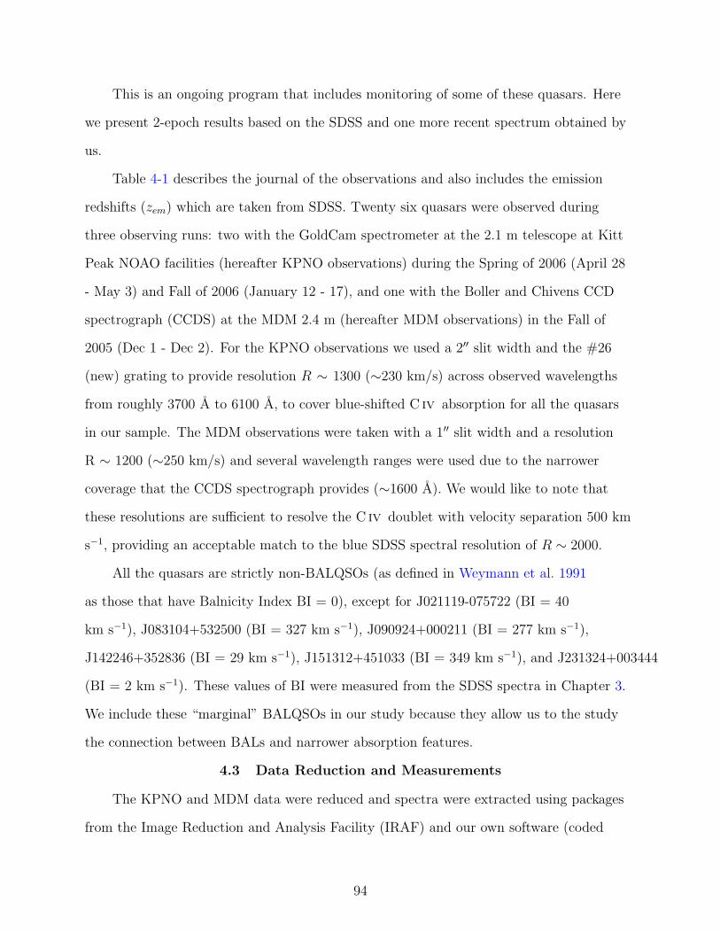
This is an ongoing program that includes monitoring of some of these quasars. Here

we present 2-epoch results based on the SDSS and one more recent spectrum obtained by

us.

Table 4-1 describes the journal of the observations and also includes the emission

redshifts (zem) which are taken from SDSS. Twenty six quasars were observed during

three observing runs: two with the GoldCam spectrometer at the 2.1 m telescope at Kitt

Peak NOAO facilities (hereafter KPNO observations) during the Spring of 2006 (April 28

- May 3) and Fall of 2006 (January 12 - 17), and one with the Boller and Chivens CCD

spectrograph (CCDS) at the MDM 2.4 m (hereafter MDM observations) in the Fall of

2005 (Dec 1 - Dec 2). For the KPNO observations we used a 2′′ slit width and the #26

(new) grating to provide resolution R ∼ 1300 (∼230 km/s) across observed wavelengths

from roughly 3700 A to 6100 A, to cover blue-shifted C iv absorption for all the quasars

in our sample. The MDM observations were taken with a 1′′ slit width and a resolution

R ∼ 1200 (∼250 km/s) and several wavelength ranges were used due to the narrower

coverage that the CCDS spectrograph provides (∼1600 A). We would like to note that

these resolutions are sufficient to resolve the C iv doublet with velocity separation 500 km

s−1, providing an acceptable match to the blue SDSS spectral resolution of R ∼ 2000.

All the quasars are strictly non-BALQSOs (as defined in Weymann et al. 1991

as those that have Balnicity Index BI = 0), except for J021119-075722 (BI = 40

km s−1), J083104+532500 (BI = 327 km s−1), J090924+000211 (BI = 277 km s−1),

J142246+352836 (BI = 29 km s−1), J151312+451033 (BI = 349 km s−1), and J231324+003444

(BI = 2 km s−1). These values of BI were measured from the SDSS spectra in Chapter 3.

We include these “marginal” BALQSOs in our study because they allow us to the study

the connection between BALs and narrower absorption features.

4.3 Data Reduction and Measurements

The KPNO and MDM data were reduced and spectra were extracted using packages

from the Image Reduction and Analysis Facility (IRAF) and our own software (coded

94

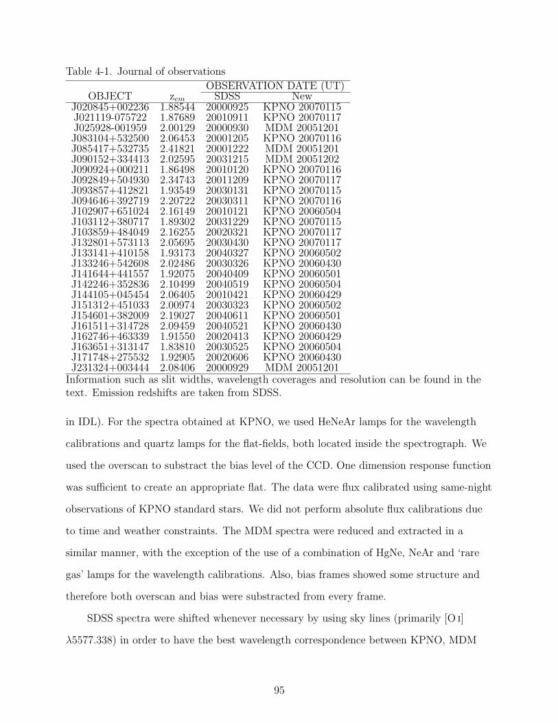
Table 4-1. Journal of observations

OBSERVATION DATE (UT)OBJECT zem SDSS New

J020845+002236 1.88544 20000925 KPNO 20070115J021119-075722 1.87689 20010911 KPNO 20070117J025928-001959 2.00129 20000930 MDM 20051201J083104+532500 2.06453 20001205 KPNO 20070116J085417+532735 2.41821 20001222 MDM 20051201J090152+334413 2.02595 20031215 MDM 20051202J090924+000211 1.86498 20010120 KPNO 20070116J092849+504930 2.34743 20011209 KPNO 20070117J093857+412821 1.93549 20030131 KPNO 20070115J094646+392719 2.20722 20030311 KPNO 20070116J102907+651024 2.16149 20010121 KPNO 20060504J103112+380717 1.89302 20031229 KPNO 20070115J103859+484049 2.16255 20020321 KPNO 20070117J132801+573113 2.05695 20030430 KPNO 20070117J133141+410158 1.93173 20040327 KPNO 20060502J133246+542608 2.02486 20030326 KPNO 20060430J141644+441557 1.92075 20040409 KPNO 20060501J142246+352836 2.10499 20040519 KPNO 20060504J144105+045454 2.06405 20010421 KPNO 20060429J151312+451033 2.00974 20030323 KPNO 20060502J154601+382009 2.19027 20040611 KPNO 20060501J161511+314728 2.09459 20040521 KPNO 20060430J162746+463339 1.91550 20020413 KPNO 20060429J163651+313147 1.83810 20030525 KPNO 20060504J171748+275532 1.92905 20020606 KPNO 20060430J231324+003444 2.08406 20000929 MDM 20051201

Information such as slit widths, wavelength coverages and resolution can be found in thetext. Emission redshifts are taken from SDSS.

in IDL). For the spectra obtained at KPNO, we used HeNeAr lamps for the wavelength

calibrations and quartz lamps for the flat-fields, both located inside the spectrograph. We

used the overscan to substract the bias level of the CCD. One dimension response function

was sufficient to create an appropriate flat. The data were flux calibrated using same-night

observations of KPNO standard stars. We did not perform absolute flux calibrations due

to time and weather constraints. The MDM spectra were reduced and extracted in a

similar manner, with the exception of the use of a combination of HgNe, NeAr and ‘rare

gas’ lamps for the wavelength calibrations. Also, bias frames showed some structure and

therefore both overscan and bias were substracted from every frame.

SDSS spectra were shifted whenever necessary by using sky lines (primarily [O i]

λ5577.338) in order to have the best wavelength correspondence between KPNO, MDM

95

and SDSS spectra. A maximum shift of 2 A has been applied and all the spectra were

shifted in the same direction, modifying the v measurents by ≤ 130 km s−1. Very accurate

v measurements are not necessary for our study and therefore we still take advantage of

the SDSS zem.

Figure 4-1 includes every observed quasar. SDSS spectra (black) are plotted over

the KPNO/MDM spectra (red). We transformed the spectra to rest wavelengths using

the SDSS zem. Some of the spectra are plotted after they underwent a 3- or 5-pixel wide

boxcar function smoothing to improve the display and facilitate comparisons between the

two spectra.

All of the spectra were normalized to unity in the continuum by a least-squares linear

fit to wavelength regions where absorption or emission were not present. This simple

normalization was sufficient to match the SDSS, MDM and KPNO spectra in the majority

of cases and throughout most of the spectral coverage of interest. However, bluewards of

4000 A (observed wavelength), the SDSS spectra sometimes deviate from the KPNO or

MDM data due to poor signal-to-noise or possibly, poor flux calibrations (J020845-002236

and J141644+441557). We do not consider those deviations to be due to variability, and

no further corrections were carried out since those deviations do not affect the absorption

features of interest here.

Following Lundgren et al. (2007), Figure 4-1 also includes values for the upper and

lower rest frame velocity boundaries of the absorption profiles in the SDSS spectrum (vmin

and vmax - dashed vertical lines in each plot). These velocities were determined by visual

inspection of each spectrum and defined as the location where the flux densities abandon

the level of the continuum.

Table 4-2 lists the results of our measurements of v, FWHM and REW on the

absorption lines. In order to extract normalized measurements of Rest Equivalent Width

(REW) and Full Width Half Minimum (FWHM), we fit a local pseudo-continuum

(continuum and emission lines) around the absorption lines by using first or second order

96

polynomial functions and Gaussians (POLYFIT in IDL and Gatorplot). Complex cases

among the present data are discussed in the Appendix.

We fit the absorption lines with one or more Gaussians, as needed, to obtain

an accurate measure of the REW. The 1σ errors in the REW listed in Table 4-2 are

dominated by the continuum placement. To estimate these errors, we manually shifted the

continuun up and down and re-measured the REW in both situations. These manual shifts

are based on visual inspection and measurements of the root-mean-square (rms) noise

in the continuum adjacent to the absorption features. The errors are our best estimates

at 1σ. We then measured the FWHM and the centroid velocities, v, directly from the

observed profiles1 . To be consistent in our measurements of NALs and mini-BALs, we

do not correct the measured FWHMs of the C iv doublet separation (∼ 500 km s−1), and

we measured FWHMs for resolved NAL doublets as if they were a single feature. Thus

the minimum FWHM we measure (for unresolved lines) is the doublet separation plus

spectral resolution, roughly 700 km s−1. Finally, we derive a dimensionless “Depth” for

every feature from the REW divided by the FWHM.

Table 4-2 lists the measurements of FWHM and v for the SDSS data only, except

for the cases where the SDSS spectra did not include any absorption but the new spectra

did, for which we list the new FWHM and v measurement. Table 4-2 also lists the REWs

for both the SDSS (REWSDSS) and the newer KPNO or MDM data (REWnew). In Table

4-2 we also include a measurement of the fractional change in the equivalent widths,

RE ≡ ∆REW/ < REW >, where ∆REW = |REWnew - REWSDSS| and < REW > is the

average value between the two epochs. As noted in Lundgren et al. (2007), these fractional

changes can be “deceptively small”. For example, features whose strengths changed

dramatically (by factors of several or more) must still have RE ≤ 2. A combination of the

1 Note that these FWHMs differ from the ones in Chapter 3, where we reportedFWHMs based on fits to the individual doublet members.

97

analysis of this parameter and visual inspection helps to discriminate between variable and

non-variable absorption and to describe better the variability when present, as we explain

in the following section.

In two instances, absorption, which was not present in the SDSS spectra, has clearly

appeared in the new observation (the absorption at λ ∼ 1395 A in J102907+651024 and

the absorption at λ ∼ 1445 A in J163651+313147, Figure 4-1). We have not included in

our list of absorption features any other differences between the SDSS and the new epoch

spectra because in every case these differences could be attributed to changes in emission

lines, variations within the noise, or they location at the edge of the spectrum, where the

flux calibration is more uncertain.

98

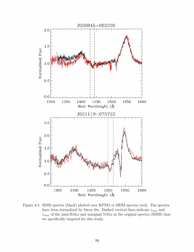
Figure 4-1. SDSS spectra (black) plotted over KPNO or MDM spectra (red). The spectrahave been normalized by linear fits. Dashed vertical lines indicate vmin andvmax of the mini-BALs and marginal NALs in the original spectra (SDSS) thatwe specifically targeted for this study.

99

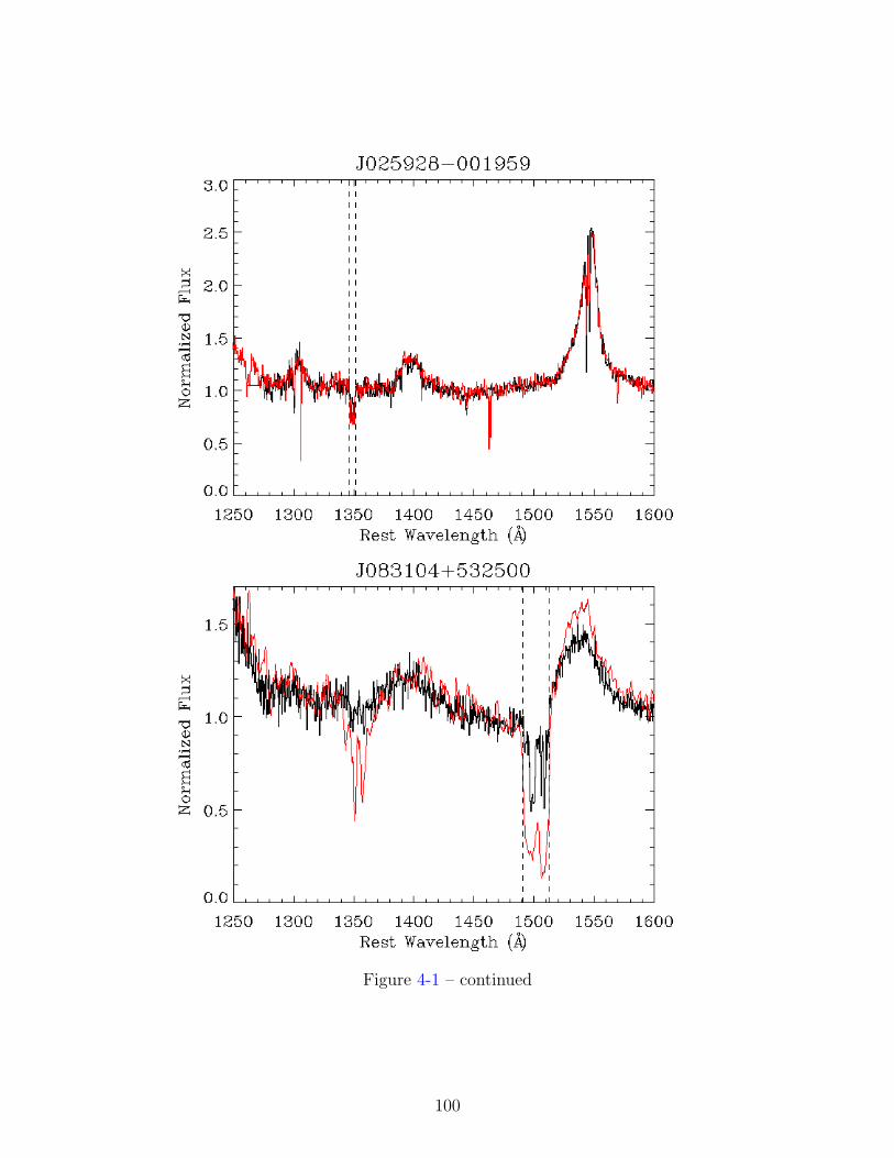
Figure 4-1 – continued

100

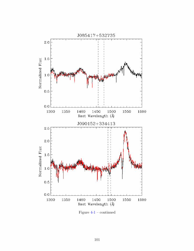
Figure 4-1 – continued

101

Figure 4-1 – continued

102

Figure 4-1 – continued

103

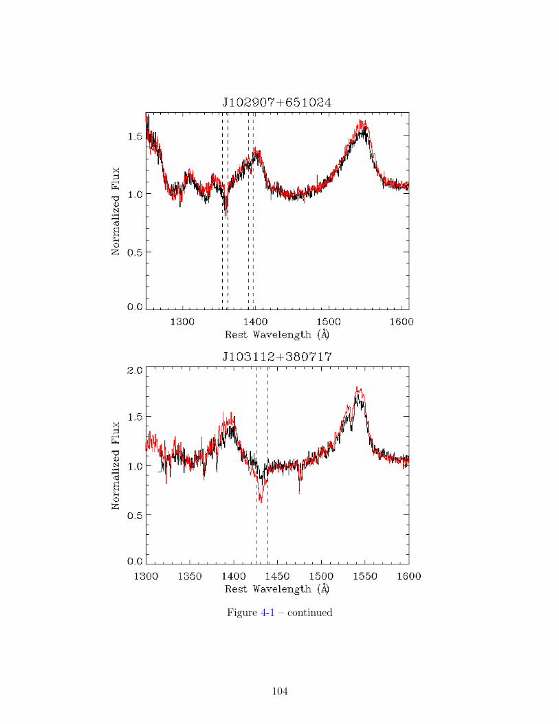
Figure 4-1 – continued

104

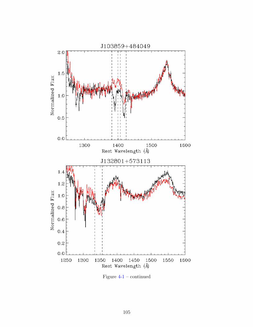
Figure 4-1 – continued

105

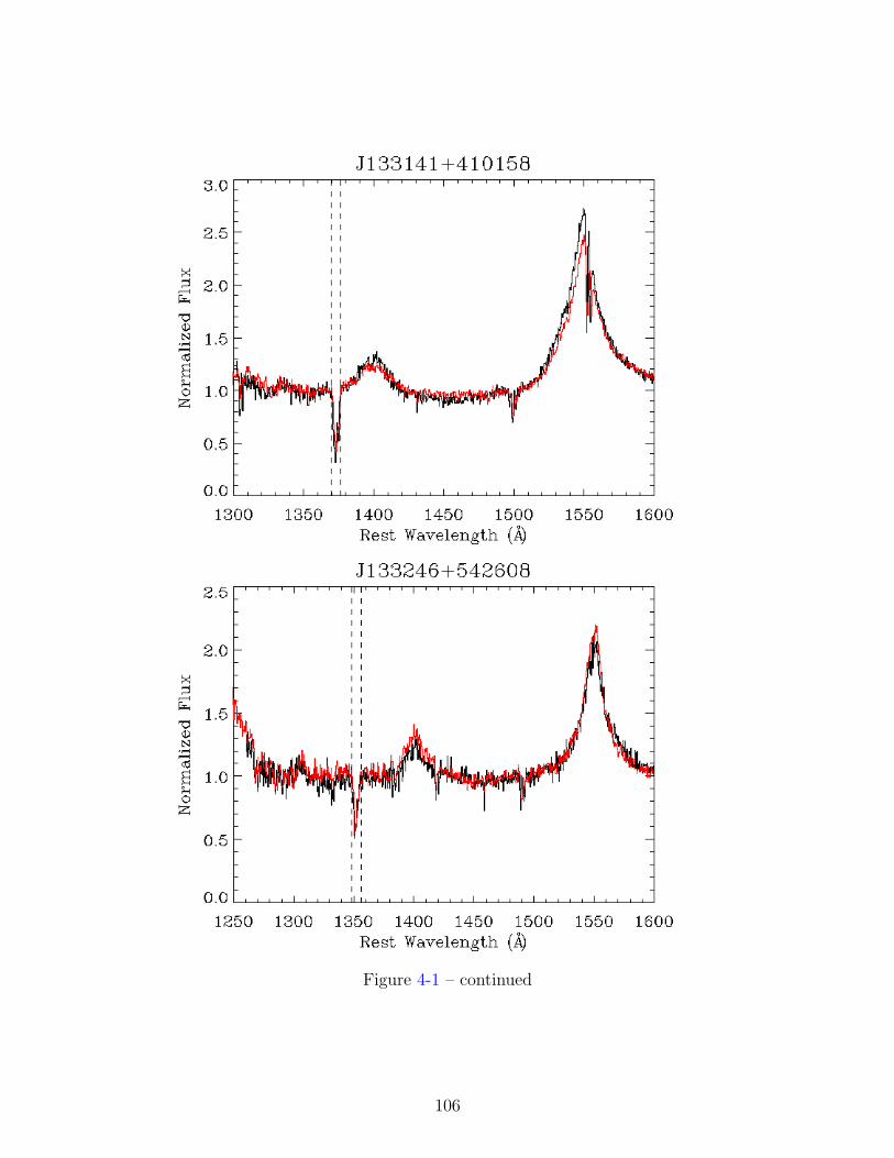
Figure 4-1 – continued

106

Figure 4-1 – continued

107

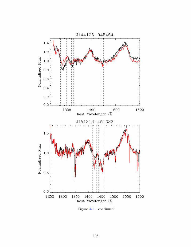
Figure 4-1 – continued

108

Figure 4-1 – continued

109

Figure 4-1 – continued

110

Figure 4-1 – continued

111

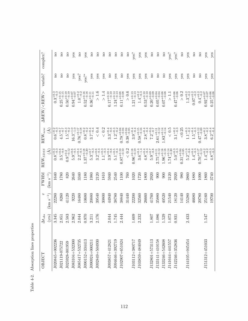
Tab

le4-

2.A

bsor

ptio

nlin

espr

oper

ties

OB

JEC

T∆

t obs

vFW

HM

RE

WS

DS

SR

EW

new

∆R

EW

/<R

EW

>va

riab

?co

mpl

ex?

(yrs

)(k

ms−

1)

(km

s−1)

(A)

(A)

J020

845+

0022

363.

345

2228

016

400.

8+0.3

−0.3

0.6+

0.2

−0.3

0.3+

0.3

−0.3

nono

J021

119-

0757

222.

851

8260

1780

3.5+

0.6

−0.6

4.5+

0.7

−0.7

0.25

+0.1

5−

0.1

5no

noJ0

2592

8-00

1959

2.58

341

120

820

0.9+

0.2

−0.1

21.

5+0.3

−0.2

0.50

+0.1

9−

0.1

9no

noJ0

8310

4+53

2300

2.96

292

2026

405.

9+0.6

−0.5

16.3

+1.0

−1.0

0.94

+0.0

7−

0.0

7ye

sye

sJ0

8541

7+53

2735

2.04

416

480

3340

2.2+

0.4

−0.4

0.76

+0.1

7−

0.1

81.

0+0.2

−0.2

yes?

noJ0

9015

2+33

4413

0.97

010

680

1180

1.37

+0.1

8−

0.2

00.

8+0.2

−0.2

0.52

+0.1

6−

0.1

6ye

s?∗

yes

J090

924+

0002

113.

211

2088

019

805.

3+0.7

−0.3

3.7+

0.4

−0.4

0.36

+0.1

1−

0.1

1ye

sno

J092

849+

5049

302.

176

3954

021

203.

2+0.6

−0.4

<0.

4>

1.6

yes

no30

800

1810

1.1+

0.3

−0.3

<0.

2>

1.4

yes

noJ0

9385

7+41

2821

2.04

444

940

5940

3.9+

0.4

−0.6

3.3+

0.4

−0.6

0.17

+0.1

0−

0.1

0no

noJ0

9464

6+39

2719

1.74

538

780

2540

5.1+

0.5

−0.4

1.2+

0.3

−0.2

1.24

+0.1

4−

0.1

3ye

sno

J102

907+

6510

242.

444

3884

011

000.

87+

0.1

0−

0.1

00.

78+

0.0

4−

0.0

40.

11+

0.0

8−

0.0

8no

no31

440

760

<0.

20.

38+

0.0

4−

0.0

5>

0.6

yes

noJ1

0311

2+38

0717

1.60

922

200

1020

0.96

+0.1

8−

0.1

93.

9+0.4

−0.4

1.21

+0.1

3−

0.1

3ye

sye

s?J1

0385

9+48

4049

2.23

232

560

1720

3.6+

0.4

−1.4

0.58

+0.1

5−

0.1

61.

4+0.2

−0.3

yes

yes

2666

018

004.

8+0.4

−0.4

2.8+

0.4

−0.4

0.53

+0.1

0−

0.1

0ye

sye

sJ1

3280

1+57

3113

1.80

741

760

2920

5.9+

0.7

−0.8

7.2+

0.6

−0.7

0.20

+0.0

9−

0.0

9no

noJ1

3314

1+41

0158

1.08

635

880

900

2.75

+0.1

1−

0.1

22.

61+

0.1

1−

0.1

20.

05+

0.0

4−

0.0

4no

noJ1

3324

6+54

2608

1.52

940

520

900

1.96

+0.1

8−

0.1

81.

83+

0.1

4−

0.1

40.

07+

0.0

8−

0.0

8no

noJ1

4164

4+44

1557

1.07

321

540

2120

1.74

+0.1

4−

0.2

0<

0.5

>1.

1ye

sye

s?J1

4224

6+35

2836

0.93

118

120

2920

5.0+

0.3

−0.3

3.1+

0.2

−0.3

0.47

+0.0

6−

0.0

6ye

sye

s?14

140

980

0.31

+0.0

4−

0.0

5<

0.25

>0.

2ye

sno

J144

105+

0454

542.

433

5528

038

605.

2+1.0

−0.6

1.1+

0.3

−0.2

1.3+

0.2

−0.2

yes

yes

4668

018

801.

4+0.4

−0.3

1.5+

0.4

−0.3

0.07

+0.2

−0.2

nono

2078

010

900.

70+

0.1

7−

0.1

20.

47+

0.1

2−

0.0

90.

4+0.2

−0.2

nono

J151

312+

4510

331.

547

2516

018

601.

4+0.2

−0.2

3.8+

0.2

−0.2

0.92

+0.0

7−

0.0

7ye

sye

s19

700

3740

4.8+

0.3

−0.3

6.2+

0.4

−0.4

0.25

+0.0

6−

0.0

6ye

sye

s

112

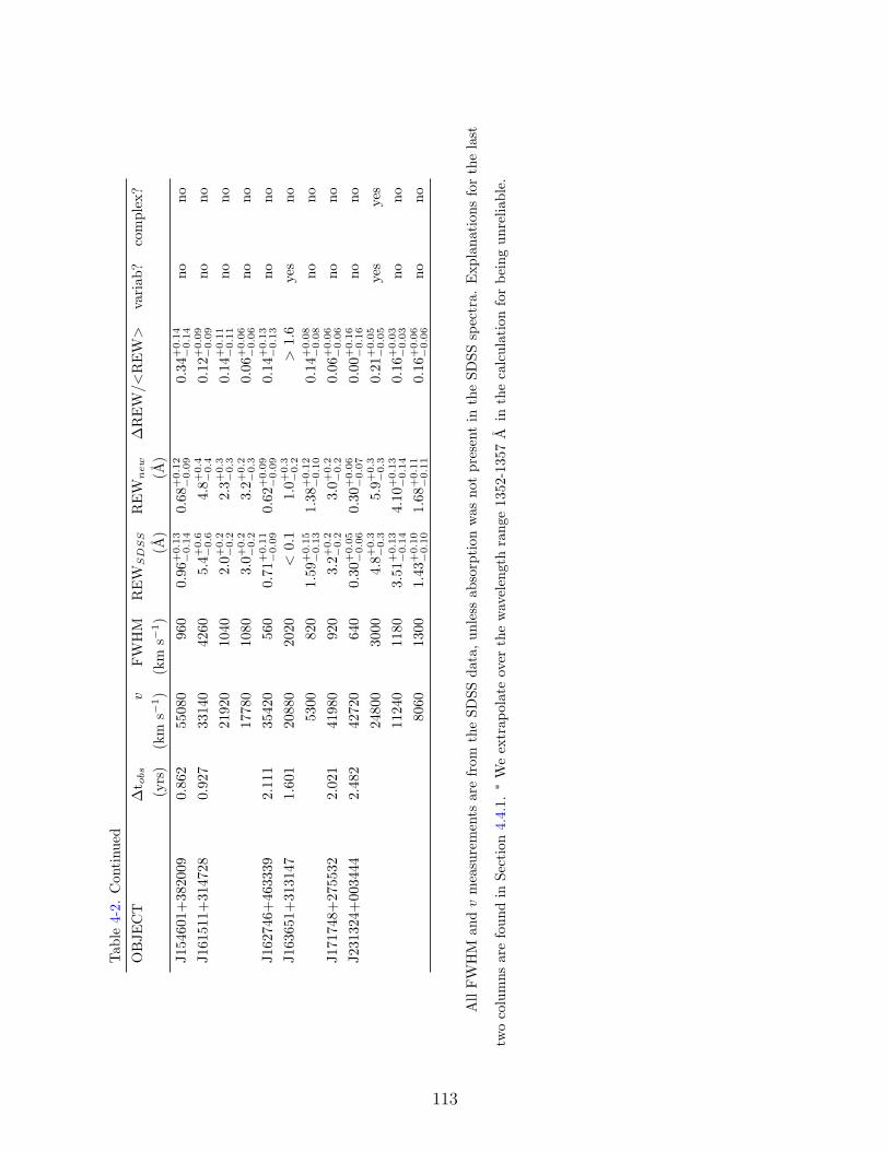
Tab

le4-

2.C

onti

nued

OB

JEC

T∆

t obs

vFW

HM

RE

WS

DS

SR

EW

new

∆R

EW

/<R

EW

>va

riab

?co

mpl

ex?

(yrs

)(k

ms−

1)

(km

s−1)

(A)

(A)

J154

601+

3820

090.

862

5508

096

00.

96+

0.1

3−

0.1

40.

68+

0.1

2−

0.0

90.

34+

0.1

4−

0.1

4no

noJ1

6151

1+31

4728

0.92

733

140

4260

5.4+

0.6

−0.6

4.8+

0.4

−0.4

0.12

+0.0

9−

0.0

9no

no21

920

1040

2.0+

0.2

−0.2

2.3+

0.3

−0.3

0.14

+0.1

1−

0.1

1no

no17

780

1080

3.0+

0.2

−0.2

3.2+

0.2

−0.3

0.06

+0.0

6−

0.0

6no

noJ1

6274

6+46

3339

2.11

135

420

560

0.71

+0.1

1−

0.0

90.

62+

0.0

9−

0.0

90.

14+

0.1

3−

0.1

3no

noJ1

6365

1+31

3147

1.60

120

880

2020

<0.

11.

0+0.3

−0.2

>1.

6ye

sno

5300

820

1.59

+0.1

5−

0.1

31.

38+

0.1

2−

0.1

00.

14+

0.0

8−

0.0

8no

noJ1

7174

8+27

5532

2.02

141

980

920

3.2+

0.2

−0.2

3.0+

0.2

−0.2

0.06

+0.0

6−

0.0

6no

noJ2

3132

4+00

3444

2.48

242

720

640

0.30

+0.0

5−

0.0

60.

30+

0.0

6−

0.0

70.

00+

0.1

6−

0.1

6no

no24

800

3000

4.8+

0.3

−0.3

5.9+

0.3

−0.3

0.21

+0.0

5−

0.0

5ye

sye

s11

240

1180

3.51

+0.1

3−

0.1

44.

10+

0.1

3−

0.1

40.

16+

0.0

3−

0.0

3no

no80

6013

001.

43+

0.1

0−

0.1

01.

68+

0.1

1−

0.1

10.

16+

0.0

6−

0.0

6no

no

All

FW

HM

and

vm

easu

rem

ents

are

from

the

SDSS

data

,un

less

abso

rpti

onw

asno

tpr

esen

tin

the

SDSS

spec

tra.

Exp

lana

tion

sfo

rth

ela

st

two

colu

mns

are

foun

din

Sect

ion

4.4.

1.∗

We

extr

apol

ate

over

the

wav

elen

gth

rang

e13

52-1

357

Ain

the

calc

ulat

ion

for

bein

gun

relia

ble.

113

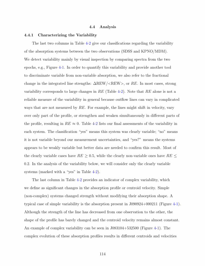
4.4 Analysis

4.4.1 Characterizing the Variability

The last two columns in Table 4-2 give our classifications regarding the variability

of the absorption systems between the two observations (SDSS and KPNO/MDM).

We detect variability mainly by visual inspection by comparing spectra from the two

epochs, e.g., Figure 4-1. In order to quantify this variability and provide another tool

to discriminate variable from non-variable absorption, we also refer to the fractional

change in the integrated line strengths: ∆REW/<REW>, or RE. In most cases, strong

variability corresponds to large changes in RE (Table 4-2). Note that RE alone is not a

reliable measure of the variability in general because outflow lines can vary in complicated

ways that are not measured by RE. For example, the lines might shift in velocity, vary

over only part of the profile, or strengthen and weaken simultaneously in different parts of

the profile, resulting in RE ≈ 0. Table 4-2 lists our final assessments of the variability in

each system. The classification “yes” means this system was clearly variable; “no” means

it is not variable beyond our measurement uncertainties, and “yes?” means the systems

appears to be weakly variable but better data are needed to confirm this result. Most of

the clearly variable cases have RE ≥ 0.5, while the clearly non-variable ones have RE ≤0.2. In the analysis of the variability below, we will consider only the clearly variable

systems (marked with a “yes” in Table 4-2).

The last column in Table 4-2 provides an indicator of complex variability, which

we define as significant changes in the absorption profile or centroid velocity. Simple

(non-complex) systems changed strength without modifying their absorption shape. A

typical case of simple variability is the absorption present in J090924+000211 (Figure 4-1).

Although the strength of the line has decreased from one observation to the other, the

shape of the profile has barely changed and the centroid velocity remains almost constant.

An example of complex variability can be seen in J083104+532500 (Figure 4-1). The

complex evolution of these absorption profiles results in different centroids and velocities

114

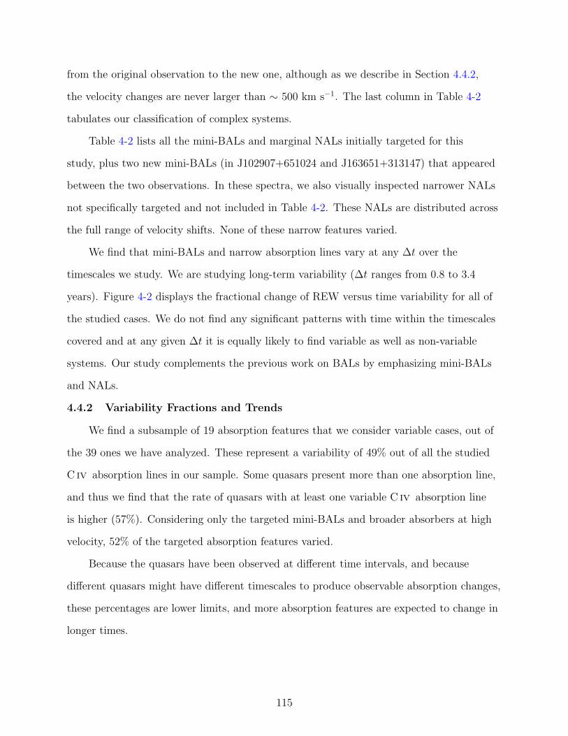
from the original observation to the new one, although as we describe in Section 4.4.2,

the velocity changes are never larger than ∼ 500 km s−1. The last column in Table 4-2

tabulates our classification of complex systems.

Table 4-2 lists all the mini-BALs and marginal NALs initially targeted for this

study, plus two new mini-BALs (in J102907+651024 and J163651+313147) that appeared

between the two observations. In these spectra, we also visually inspected narrower NALs

not specifically targeted and not included in Table 4-2. These NALs are distributed across

the full range of velocity shifts. None of these narrow features varied.

We find that mini-BALs and narrow absorption lines vary at any ∆t over the

timescales we study. We are studying long-term variability (∆t ranges from 0.8 to 3.4

years). Figure 4-2 displays the fractional change of REW versus time variability for all of

the studied cases. We do not find any significant patterns with time within the timescales

covered and at any given ∆t it is equally likely to find variable as well as non-variable

systems. Our study complements the previous work on BALs by emphasizing mini-BALs

and NALs.

4.4.2 Variability Fractions and Trends

We find a subsample of 19 absorption features that we consider variable cases, out of

the 39 ones we have analyzed. These represent a variability of 49% out of all the studied

C iv absorption lines in our sample. Some quasars present more than one absorption line,

and thus we find that the rate of quasars with at least one variable C iv absorption line

is higher (57%). Considering only the targeted mini-BALs and broader absorbers at high

velocity, 52% of the targeted absorption features varied.

Because the quasars have been observed at different time intervals, and because

different quasars might have different timescales to produce observable absorption changes,

these percentages are lower limits, and more absorption features are expected to change in

longer times.

115

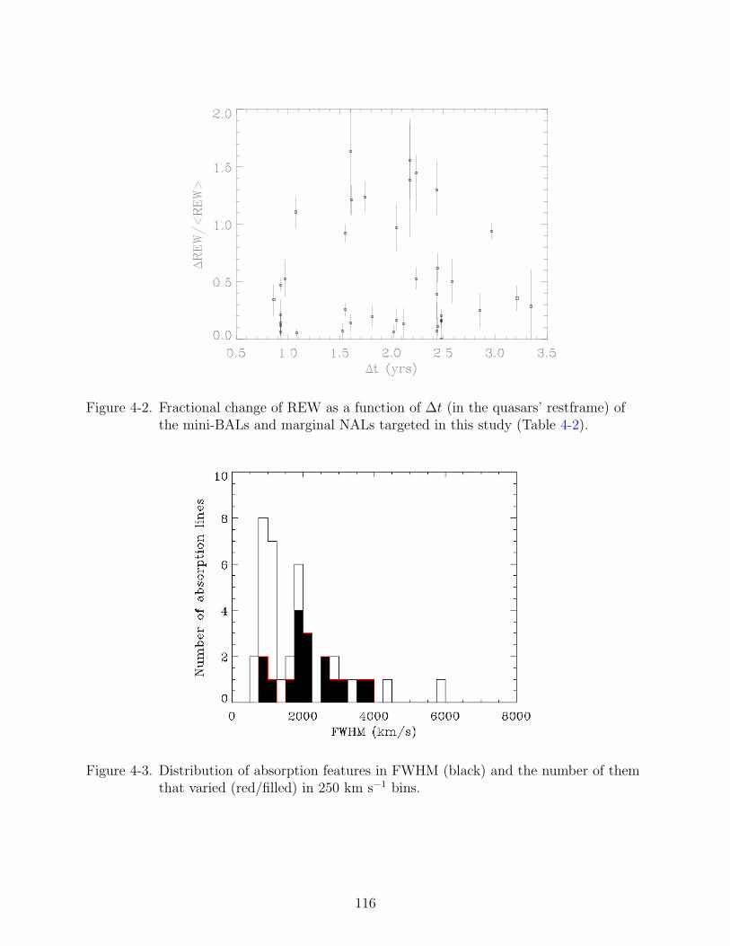
Figure 4-2. Fractional change of REW as a function of ∆t (in the quasars’ restframe) ofthe mini-BALs and marginal NALs targeted in this study (Table 4-2).

Figure 4-3. Distribution of absorption features in FWHM (black) and the number of themthat varied (red/filled) in 250 km s−1 bins.

116

Figures 4-3 to 4-5 show the number of systems that varied versus their FWHM, depth

and v of the absorption. Figure 4-3 displays the distribution in FWHM, as tabulated

in Table 4-2, of the number of cases that varied (red/filled) versus the total number of

absorption features included in our study in 500 km s−1 bins. As we mentioned earlier,

our goal is two-fold; one objective is to confirm, through variability, the intrinsic nature

of the narrowest systems in our sample which might or might not be outflows. As Figure

4-3 shows, the majority of systems with 500 < FWHM < 1000 km s−1 remains invariable,

and absorption lines are more prone to vary if they have FWHM > 1500 km s−1. The

Kolmogorov-Smirnov (KS) test probability that the FWHM in both distributions (all

cases and only variable cases) are drawn from the same population is 0.17. However, if

we select only those systems with FWHM > 1500 km s−1, the KS probability is 0.9993,

which implies consistency between the two populations. For the systems with FWHM

< 1500 km s−1, the difference between the two populations (all cases and only variable

cases) is larger than 3 σ, which suggests that they are drawn from different populations.

We have confirmed the outflow nature of two cases with 500 < FWHM < 1000 km s−1

that have varied (lowest velocity absorption lines in the spectra of J102907+651024 and

J142246+352836, Figure 4-1).

Figure 4-4 presents the distribution of C iv absorbers versus their depth for the full

sample (black) and those cases that varied (red line/filled). There is no obvious trend in

the variability versus line depth. The KS test probability of both populations (the depths

of only variable cases and all cases) being drawn from the same distribution is 0.9995,

which suggests consistency between the two populations.

The second goal of this work is to characterize the variability of confirmed outflows,

excluding intervening material. Figure 4-5 shows the total number of studied outflows

at each velocity (black) and the number of outflows that varied (red/filled) in velocity

bins of 5000 km s−1. We have included only those absorption features that are very likely

outflows: all of the cases with FWHM > 1000 km s−1 and those narrower absorption lines

117

Figure 4-4. Distribution of absorption features in depth (black) and the number of themthat varied (red/filled) in 0.05 bins.

Figure 4-5. Distribution of absorption features in velocity (black) and the number of themthat varied (red/filled) in 5000 km s−1 bins.

118

that also varied. C iv absorption with FWHM > 1000 km s−1 is unlikely to be part of

intervening material (Chapter 32 ). We do not find any significant trend with velocity. The

KS test probability that the v for the variable cases and all cases are drawn from the same

population is 0.63, which suggests consistency between the two populations.

Figure 4-6. Fractional change of REW versus average REW of all the absorption lines inour sample

In Figure 4-6 we represent the absolute fractional change of REW versus averaged

REW for comparison with Lundgren et al. (2007). We find that only features with

<REW> < 4 A (approx. 900 km s−1) show absolute fractional changes in REW larger

than 1, values which are within the errors.

2 In Chapter 3 we used a lower limit of FWHM ≥ 700 km s−1 for the higher oscillationstrength individual line of the C iv doublet while in this work we are using a characteristicFWHM for the whole doublet profile

119

Figure 4-7. Fractional change of REW versus depth of all the absorption lines in oursample

Figure 4-7 is similar to Figure 4-6, but we plot depth instead of <REW>. As we find

in Figure 4-6, there are not absorption features with ∆REW/<REW> larger than 1 for a

certain value of depth (depth ∼> 0.5).

The large variety of velocities of the absorption features in our sample allows us to

search for trends of this property with variability. Figure 4-8 displays the fractional change

of REW versus velocity. This figure shows that both variable and non-variable absorption

features are observed at every velocity. There is not a narrow range of velocity where the

largest ∆EW/<EW> occur.

Figures 4-9 and 4-10 display velocity and velocity width (defined as vmax−vmin) versus

depth for the cases we have found to vary. In Figure 4-9, the arrows connect vwidth and

depth in the SDSS data to the values of those quantities in the second observation. Figure

4-9 shows that in the large majority of variable cases, changes in depth and in velocity

width occur in the same direction, i.e., whenever the depth increases/decreases, the vwidth

increases/decreases as well, respectively. Absorption features in quasars J103112+380717

120

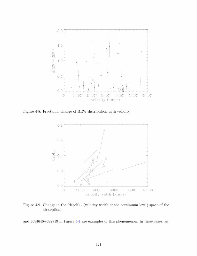
Figure 4-8. Fractional change of REW distribution with velocity.

Figure 4-9. Change in the (depth) - (velocity width at the continuum level) space of theabsorption.

and J094646+392719 in Figure 4-1 are examples of this phenomenon. In these cases, as

121

the absorption feature increases in strength, it also widens at the base of the absorption

(continuum level), thereby covering a larger range of absorbed velocities.

Figure 4-10. Change in (depth) - (velocity) space of the absorption.

We do not find significant changes in the velocity of the absorption in any of the

variable cases. In every studied case, variability occurs primarly in strength. There are

no cases showing clear displacement of the absorption feature as ‘a whole’, as reported

in Gabel et al. (2003) (shown in their Figure 2), where a feature seems to decelerate by

∼ 100 km s−1 in 1.8 years. Figure 4-10 shows how the v is very steady in variable cases.

Slight variations in velocity are mostly caused by the complexity of some absorption

profiles, which complicates the determination of the centroid and thus the central velocity,

as we described in §4.4.1.

If several absorption features were present in one quasar spectrum and one of

these features varied, then the others either did not vary or they varied in the same

direction (increase/decrease if the original increase/decrease). For example, in the case of

J151312+451033 (Figure 4-1), the absorption at ∼ 1415 A increases significantly while the

absorption centered at ∼ 1500 A did not suffer such a dramatic change.

122

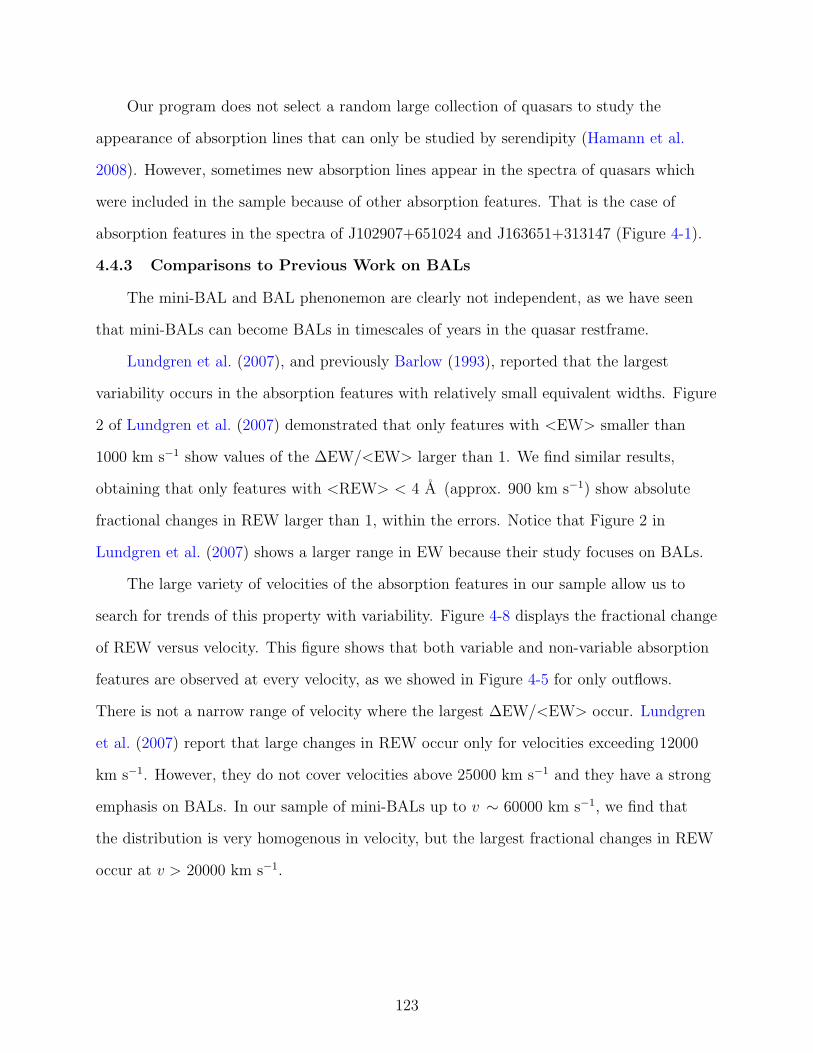
Our program does not select a random large collection of quasars to study the

appearance of absorption lines that can only be studied by serendipity (Hamann et al.

2008). However, sometimes new absorption lines appear in the spectra of quasars which

were included in the sample because of other absorption features. That is the case of

absorption features in the spectra of J102907+651024 and J163651+313147 (Figure 4-1).

4.4.3 Comparisons to Previous Work on BALs

The mini-BAL and BAL phenonemon are clearly not independent, as we have seen

that mini-BALs can become BALs in timescales of years in the quasar restframe.

Lundgren et al. (2007), and previously Barlow (1993), reported that the largest

variability occurs in the absorption features with relatively small equivalent widths. Figure

2 of Lundgren et al. (2007) demonstrated that only features with <EW> smaller than

1000 km s−1 show values of the ∆EW/<EW> larger than 1. We find similar results,

obtaining that only features with <REW> < 4 A (approx. 900 km s−1) show absolute

fractional changes in REW larger than 1, within the errors. Notice that Figure 2 in

Lundgren et al. (2007) shows a larger range in EW because their study focuses on BALs.

The large variety of velocities of the absorption features in our sample allow us to

search for trends of this property with variability. Figure 4-8 displays the fractional change

of REW versus velocity. This figure shows that both variable and non-variable absorption

features are observed at every velocity, as we showed in Figure 4-5 for only outflows.

There is not a narrow range of velocity where the largest ∆EW/<EW> occur. Lundgren

et al. (2007) report that large changes in REW occur only for velocities exceeding 12000

km s−1. However, they do not cover velocities above 25000 km s−1 and they have a strong

emphasis on BALs. In our sample of mini-BALs up to v ∼ 60000 km s−1, we find that

the distribution is very homogenous in velocity, but the largest fractional changes in REW

occur at v > 20000 km s−1.

123

4.5 Discussion

We have presented results from a 2-epoch observational study of 26 quasars selected

for having either mini-BALs or weak BALs (certain outflow lines) or marginal/broad

NALs (candidate outflow lines). Our main goals are to characterize the variability

properties of the outflow features and test the possible outflow origin of the candidate

NALs and other NALs present in the spectra. We are particularly interested in mini-BALs

and other narrow outflow features in order to establish a comparison to previous work on

variability in BALs (Barlow 1993; Lundgren et al. 2007; Gibson et al. 2008).

4.5.1 Summary of Main Results

• We find that 49% out of the 39 studied C iv absorption lines in our sample vary overa range of ∆tobs = 0.9 - 3.3 years in the quasar rest frame. Out of the 26 studiedquasars, this represents a percentage of 57% quasars that include at least one variableabsorption feature. Considering only the targeted mini-BALs and broader absorbersat high velocity, 52% of the targeted absorption features varied.

• We find that 58% of the variable cases show complex variability.

• The variability occurs at all studied velocities (from 5000 to 60000 km s−1) and wedo not conclusively find any trend between the fractional change of the absorption(∆REW/<REW>) and v.

• We do not find any trends with REW or depth, except that there is not variability ofthe absorption features with largest depths, which occur in narrow systems.

• Except for the case of J144105+045454, none of the studied variable featuresshow shifts in velocity larger than 1000 km s−1. Although the centroid velocitiesgenerally shift between observations in the complex cases, there is no clear evidencefor acceleration or deceleration of gas in the flow

• None of the narrow systems with FHWM < 700 kms −1 varied in our data. Thisproperty might suggest that very strong narrow absorption tends to be intervening.

• The mini-BAL and BAL phenomenon are clearly not independent, as we have seenthat mini-BALs can become BALs in timescales of years in the quasar restframe.

4.5.2 Physical Properties of the Absorbers and Variability Causes

In this section we discuss how the results above help to place constraints on the

absorber physical properties and the causes of the observed variability. Previous studies on

124

this matter, i.e., Misawa et al. (2005) and Narayanan et al. (2004), describe the possible

causes of mini-BAL variability.

4.5.2.1 Change of the ionization state

Changes in the ionizing continuum flux can cause changes in the ionization state of

the outflow absorbers, leading to changes in the absorption line strengths. Weak outflow

lines like NALs and mini-BALs might be more susceptible to this effect than BALs if the

former are generally less saturated.

We are not able to determine whether variations in the level of the continuum

ionization are the cause of the C iv absorption variability mainly because of three issues.

First, we cannot measure the continuum flux because we do not have absolute flux

calibrations for the KPNO and MDM spectra. Moreover, this information would still

not measure the ionizing flux in the UV/soft X-ray continuum. Second, we only have

information regarding one ionic species (C iv) and we cannot determine the ionization

of the outflows. Third, there might be a delay between the time the continuum reaches

the absorber and the absorber variations (recombination time). We have carried out such

a study for J093857+412821, which has been described in Chapter 2. Barlow (1993),

Lundgren et al. (2007) and Gibson et al. (2008) found no correlations between the

continuum flux level and the absorption changes.

If we assume that the variability is caused by the ionization changes, then we can

place limits on the minimum electron density (ne) and the maximum distance from the

continuum source. To do so, we need to resort to some assumptions: the changes in the

continuum are small, the gas is in ionization equilibrium, C iv is the dominant ionization

species of C , and that the temperature of the gas is T ∼ 20000 K (Hamann et al. 1997a;

Narayanan et al. 2004).

Using Eq. (1) in Narayanan et al. (2004), our observed variability times provide upper

limits on the recombination times. We have found that the C iv absorption varies in a

wide range of variability times. Most importantly, we have not found an observed time

125

after which every outflowing C iv absorber varies. Variability times are included in Table

4-2 and have been discussed further in §4.4.1. Assuming a typical variability timescale

of 2.0 years, we can derive a minimum electron density ne ∼> 5700 cm−3. The shortest

observed variability timescale (0.97 yrs) will result in ne ∼> 11600 cm−3.

These electron densities allow us to derive the maximum distance between the

absorbing clouds and the continuum source by assuming the gas is in photoionization

equilibrium with an ionization parameter and continuum shape (Narayanan et al. (2004)

eq. [2]). For this, we also need to assume that the absorbing clouds are not “shielded”

from the continuum emission source. Thus, the gas is receiving the whole flux of ionizing

photons scaled by 1/R2. By using a typical luminosity for the quasars in our sample

(Lbol ∼ 5 x 1046 erg s−1), and an ionizing parameter U ≈ 0.02 (optimal for C iv), we

obtain a maximum distance between the absorbers and the source of the ionization

continuum of ≤ 2 kpc.

We find that sometimes in the same spectrum absorption at some velocity varies

significantly while absorption in the same spectrum at another velocity remains almost

constant (description in §4.4.2). If variability is due to changes in the ionizing continuum,

both absorbers should be affected by the ionization changes in the same manner, unless

they are either 1) at different distances (e.g., the invariable absorption is produced by an

absorber(s) that must be located at a distance r > 2 kpc from the continuum, while the

variable is related to an absorber which must be closer), or 2) the invariable absorption

is saturated. None of the mini-BAL or narrow lines in spectra of our quasar sample

goes black, which means that if they are saturated, the absorbers must be only partially

covering the emission source.

We have found absorption that remains constant over long timescales (> 3 years) in

the quasar restframe. If the ionizing continuum has varied during this time, and assuming

we have not randomly caught it at the same stage at both observations, the lack of

126

variation in the absorption troughs might indicate that the absorber(s) is(are) too tenuous

to respond on continuum variation timescales.

4.5.2.2 Motion of the absorber

Variability can also be caused by transverse bulk motion of the absorber. Variability

timescales in this case correspond to crossing time of the absorber(s) across the emitting

background source (which would produce variations in the covering factors of the gas).

The background sources could be the Broad Emission Line Region (BELR) and/or

the continuum source ( Ganguly et al. 1999). Typical sizes for the BELR of the quasars

in our sample are derived from the empirical relation between them and the quasar

luminosity (Vestergaard 2002), obtaining ∼ 3pc. The continuum source size that is

producing most of the continuum can be estimated to be 5RS = 10GMBH/c2 (Misawa

et al. 2005), where RS and MBH are the Schwarzschild radius and the black hole mass,

respectively. We derive MBH from the relation between FWHM of the C iv emission line

and the luminosity at 1450 A, (Warner et al. 2003). Typical values for MBH in the quasars

of our sample are 109-1010 M¯. Therefore, we obtain typical radial sizes of the continuum

source to be ∼ 0.0005 - 0.005 pc.

By assuming a simple geometry, we can obtain lower limits for the transverse velocity

vtr of the absorber in the cases where the absorption has appeared/disappeared. Imagine a

homogenous background source as a square of side 2r, and another square outflow passing

across it. In order to show variability in the absorption, the absorber should travel a

transverse distance Cf × 2r, where Cf is the covering factor. For example, in the case

of the absorption at a rest wavelength of ∼ 1440 A in the spectrum of J141644+441557

(Figure 4-1), the absorption is present in the SDSS spectrum but it has disappeared in the

KPNO one. We have an upper limit for the variability time, given by the time difference

between the two observations: ∼ 1 yr. Because the depth of the normalized absorption

indicates that Cf is ≥ 0.15 (15% of the emitting source), the distance that the absorber

(assuming sharp edges) needs to travel in order to abandon the line of sight is ∼ 5 × 1012

127

- 5 × 1015 cm (0.00015 - 0.0015 pc). In 1 year, this distance can be travelled by absorbers

moving at transverse speeds of vtr > 150 - 1500 km s−1. These values are comparable to

the disk rotation speeds just beyond RCIV, vtr ∼ 3000 km s−1. However, in order to cross

the same area of the BLR (radius ∼ 3 pc), we would need speeds larger than the speed of

light, as was obtained for the outflow in HS 1603+3820 studied in Misawa et al. (2005).

Therefore, we conclude that the absorber covers primarily the UV continuum source and,

maybe, only a small part of the BLR (Misawa et al. 2005).

128

CHAPTER 5SUMMARY AND CONCLUSIONS

Outflows are a fundamental part of quasars: they bring first-hand physical information

about the quasar environments, they are common (and maybe ubiquitous) and they might

be key to connect the AGN with their host galaxies. However, many aspects of these

outflows (e.g., acceleration mechanisms, geometry, evolution) are poorly understood.

I present new measurements and analyses of these absorption lines in the spectra

of the quasar PG0935+417 (zem ≈ 1.966). This quasar shows a high velocity C iv

mini-Broad Absorption Line (mini-BAL) outflowing at ∼51000 km s−1. We detect,

using Lick observatory, Hubble Space Telescope, and Sloan Digital Sky Survey spectra,

absorption in C iv λλ1548,1551 (already reported in Hamann et al. 1997a and Narayanan

et al. 2004) and, for the first time in this outflow, absorption in Nv λλ1240 and Ovi

λλ1034 in this mini-BAL system. The absence of lower ionization lines indicates that

the flow is highly ionized with an ionization parameter log U ∼> -1.1. The resolved Ovi

indicates that the lines are moderately saturated with the absorber, covering just ∼80% of

the background continuum source. We estimate the total column density to be NH ∼> 3.0

x 1019 cm−2, which is small enough to be compatible with radiation pressure mechanisms

accelerating this outflow.

I also have contributed to the study of outflows by focusing in a realm of the

parameter space that has been sparsely surveyed before: mini-broad absorption lines

(mini-BALs) and high velocities outflows (v ∼> 10000 km s−1). My goals are to 1)

quantitatively define the range of outflow lines in quasar spectra, 2) examine their

detection frequencies and distributions in velocity, strength and FWHM, 3) look for

relationships between the various absorption line types and basic quasar properties, and

4) identify individual outflow line candidates for follow-up studies. To do so, I compile a

comprehensive catalog of C iv absorption lines in the ∼ 2000 brightest SDSS quasars at

1.8≤ z ≤3.5, and select those with FWHM > 700 km s−1 to be unlikely due to intervening

129

material. I obtain a fraction of quasars with mini-BALs of 11.4%±0.9%. Although

the mini-BAL phenomenon is strongly related to the more previously studied Broad

Absorption Lines (BALs) present in BALQSOs, we still find mini-BALs in 5.1%±0.7%

of non-BALQSOs. I find no correlation between the presence of associated absorbers or

radio loudness and the occurance of mini-BALs. By adding results from other outflow

studies to my results, I estimate a total percentage of quasars with outflows to be ∼41–77%. Mini-BALs pose a unique challenge for outflow models because they can have

large outflow velocities, v, with small velocity dispersions, FWHM. BALs and mini-BALs

might represent an evolutionary sequence, a single outflow structure viewed at different

angles, or some combination of these scenarios. In either case, the detection frequencies

reported here provide important constraints on the relative lifetimes or opening angles of

the different outflow types.

Finally, to characterize better the structural and physical properties of these outflows,

I carried out a monitoring program over a range of ∆t = 0.9 -3.3 years in the quasar rest

frame, using facilities at the Kitt Peak National Observatory and MDM Observatory. By

comparing our new spectra with archival spectra (SDSS) I find that ∼ 50% of quasars

with mini-BAL and BALs at high velocity varied between just two observations. I find

that variability sometimes occurs in complex ways. All the observed variations occur in

intensity and not in velocity. Thus I find no evidence for acceleration/deceleration in the

outflow. I also do not find any correlations between the variability and Rest Equivalent

Width (REW), Full Width Half Minimum (FWHM) or depth of the absorption feature,

except for the fact that most of the narrowest systems did not vary. A significant fraction

of the non-variable narrower systems are probably unrelated to quasar outflows.

130

APPENDIX: ADDITIONAL OBSERVATIONS

A.1 J083104+532500

The original marginal complex mini-BAL/BAL (FWHM = 2640 km s−1) in this

quasar (BI = 327 km s−1) has increased its strength in both the C iv and the Si iv

absorption. The absorption in the SDSS spectrum was composed of three different

structures: two strong narrow lines (FWHM of the individual lines ∼< 500 km s−1)

superposed on a weaker wider absorption feature. The new absorption profile retains

some of the two troughs but it is impossible to know which of the original three absorption

lines has gotten stronger. The presence of several narrow (FWHM ∼ 600 km s−1) Si iv

absorption lines also suggests that the C iv absorption should be still be composed of

several components. There is very likely an effect of partial covering. We support this

idea for two reasons. First, the doublet ratio of the Si iv doublet line at λ 1350-1360 A

does not show the expected 2:1 ratio in optical depth, which it should if not saturated.

Second, the optical depth in C iv should be at least 5 times larger than Si iv if the Si/C

abundance is roughly solar and Si iv and C iv are the optimal ions present (Hamann et al.

1997c; Hamann & Ferland 1999; Hamann et al. 2008). Partial coverage is commonly found

in NALs (i.e., Hamann et al. 1997c; Ganguly et al. 1999; Arav et al. 2001; Hamann &

Sabra 2004), and in BALs (Arav et al. 1999).

A.2 J092849+504930

The absorber at λ ∼ 1395 A was not originally in our sample of mini and broad

absorption lines in quasars (Chapter 3 because of the possibility of being attributed to

the separation between the Si iv and the O iv emission lines and not to ‘real’ absorption.

However, we include it in this work because its variation between the two epochs (Figure

4-1) seems not to be due to changes in the emission lines, especially since the C iv

emission line and the rest of the Si iv+O iv do not vary.

131

A.3 J093857+412821

We have been monitoring this quasar due to its very variable absorption at ∼ 50000

km s−1. For more information go to Chapter 2.

A.4 J102907+651024

This quasar was observed because of its other absorption lines. However, an

absorption line has seemed to have appeared at λ ∼ 1395 A. Although narrow, its

width (FWHM = 760 km s−1) makes it unlikely to be caused by other ions. The fact that

the C iv emission line wis increasing in strength while keeping its shape suggests that the

trough in the Si iv+O iv emission line is not caused by a decrease in the intensity of this

complex emission lines, and therefore we have included the line as an absorption feature.

A.5 J103859+484049

The SDSS spectrum shows an almost flat pseudo-continuum (continuum + emission

lines) in the region where the Si iv emission lines is supposed to be. The strength of the

C iv emission line and the fact that it does not change between the two observations,

suggests that the C iv absorption in the spectral range λ ∼1380 - 1420 A is strong enough

to be absorbing both the continuum and the emission line. In order to determine the

correct normalized strength of the absorption in both spectra, we fitted a Gaussian to

the KPNO spectrum by outlining it through the highest intensity regions in the range

λ ∼1380 - 1420 A. This method results in a conservative measurement of the strengths

of all the absorption in that region, since the emission could be stronger than we predict.

Si iv absorption lines are present in the same outflow.

Si iv absorption lines are present in the same outflow. Visual inspection of that region

suggests that at least the absorber at zabs ∼ 1.89 (C iv at λ∼ 1415 A) is accompanied

by Si iv absorption at λ∼ 1275 A. The strength of the Si iv doublet, which should

be at least 5 times weaker than C iv if the Si/C abundance is roughly solar and the

optimal ions are Si iv and C iv, suggests that C iv must be saturated because of an effect

132

of partial covering, as it happened in J083104+532500 (above) and the SDSS quasar

J105400+034801 (Hamann et al. 2008).

A.6 J144105+045454

Figure A-1. Normalized SDSS spectra (black) and KPNO spectra (red/grey)

This quasar is an example of what we define as complex absorption variability. The

absorption is present in the spectral region λ∼ 1270 - 1335 A. The presence of Si iiλ1260

and O iλ1302 emission lines intertwined with the absorption forced us to fit Gaussians

to these emission features before measuring. We fit one Gaussian per emission line of

the KPNO spectrum, where the O i emission line is more noticeable. We used this fit to

normalize both SDSS and KPNO spectra, assuming that the emission line has not varied

between both observations. Figure A-1 shows both normalized spectra. Assuming that

there are two distinctive absorption troughs (one at λ∼ 1270 - 1305 A and other at λ∼1305 - 1330 A), both absorption features might have redshifted its centrod (produced

by acceleration). However, further study is necessary because of the complexity of the

variability of this absorption profile.

133

A.7 J163651+313147

As in the case of J102907+651024, this quasar was observed at KPNO because of its

narrow absorption lines. However, a mini-BAL has seemed to have appeared at λ ∼ 1445

A. This absorption line seems far enough from the Si iv emission line to not be attributed

to ‘real’ absorption. Notice, however, the difference between the Si iv emission lines in

both spectra.

134

REFERENCES

Adelman-McCarthy, J. K. and Agueros, M. A. and Allam, S. S. and Allende Prieto, C.and Anderson, K. S. J. and Anderson, S. F. and Annis, J. and Bahcall, N. A. andBailer-Jones, C. A. L. and Baldry, I. K., et al. 2008, ApJS, 175, 297

Aldcroft, T. L., Bechtold, J., & Elvis, M. 1994, ApJS, 93, 1

Anderson, S. F., Weymann, R. J., Foltz, C. B., & Chaffee, F. H., Jr. 1987, AJ, 94, 278

Arav, N., Becker, R. H., Laurent-Muehleisen, S. A., Gregg, M. D., White, R. L.,Brotherton, M. S., & de Kool, M. 1999, ApJ, 524, 566

Arav, N., de Kool, M., Korista, K. T., Crenshaw, D. M., van Breugel, W., Brotherton, M.,Green, R. F., Pettini, M., Wills, B., de Vries, W., Becker, B., Brandt, W. N., Green, P.,Junkkarinen, V. T., Koratkar, A., Laor, A., Laurent-Muehleisen, S. A., Mathur, S., &Murray, N. 2001, ApJ, 561, 118

Arav, N., Li, Z.-Y., & Begelman, M. C. 1994, ApJ, 432, 62

Baker, J. C., Hunstead, R. W., Athreya, R. M., Barthel, P. D., de Silva, E., Lehnert,M. D., & Saunders, R. D. E. 2002, ApJ, 568, 592

Barlow, T. A. 1993, Ph.D. thesis, AA(California Univ.)

Barlow, T. A., & Sargent, W. L. W. 1997, AJ, 113, 136

Becker, R. H., Gregg, M. D., Hook, I. M., McMahon, R. G., White, R. L., & Helfand,D. J. 1997, ApJ, 479, L93

Becker, R. H., White, R. L., Gregg, M. D., Brotherton, M. S., Laurent-Muehleisen, S. A.,& Arav, N. 2000, ApJ, 538, 72

Becker, R. H., White, R. L., & Helfand, D. J. 1995, ApJ, 450, 559

Bennett, A. S. 1962, MmRAS, 68, 163

Bregman, J. N., Glassgold, A. E., Huggins, P. J., Neugebauer, G., Soifer, B. T., Matthews,K., Elias, J. H., Webb, J. R., Pollock, J. T., Leacock, R. J., Smith, A. G., Aller,H. D., Aller, M. F., Hughes, P. A., Maccagni, D., Garilli, B., Giommi, P., Miller, J. S.,Stephens, S., Balonek, T. J., Dent, W. A., Kinsel, W., Wisniewski, W. Z., Williams,P. M., Brand, P. W. J. L., & Ku, W. H.-M. 1990, ApJ, 352, 574

Brotherton, M. S., Laurent-Muehleisen, S. A., Becker, R. H., Gregg, M. D., Telis, G.,White, R. L., & Shang, Z. 2005, AJ, 130, 2006

Brotherton, M. S., van Breugel, W., Smith, R. J., Boyle, B. J., Shanks, T., Croom, S. M.,Miller, L., & Becker, R. H. 1998, ApJ, 505, L7

Canalizo, G., & Stockton, A. 2001, ApJ, 555, 719

135

Canalizo, G., & Stockton, A. 2002, in Astronomical Society of the Pacific ConferenceSeries, 255, Mass Outflow in Active Galactic Nuclei: New Perspectives, ed. D. M.Crenshaw, S. B. Kraemer, & I. M. George, 195

Capellupo, D., & Hamann, F. 2009, ApJ(in prep.)

Churchill, C. W., Schneider, D. P., Schmidt, M., & Gunn, J. E. 1999, AJ, 117, 2573

Crenshaw, D. M., & Kraemer, S. B. 2007, ApJ, 659, 250

Crenshaw, D. M., Kraemer, S. B., Boggess, A., Maran, S. P., Mushotzky, R. F., & Wu,C.-C. 1999, ApJ, 516, 750

Crenshaw, D. M., Kraemer, S. B., & George, I. M. 2003, ARA&A, 41, 117

Croton, D. J., Farrar, G. R., Norberg, P., Colless, M., Peacock, J. A., Baldry, I. K.,Baugh, C. M., Bland-Hawthorn, J., Bridges, T., Cannon, R., Cole, S., Collins, C.,Couch, W., Dalton, G., De Propris, R., Driver, S. P., Efstathiou, G., Ellis, R. S., Frenk,C. S., Glazebrook, K., Jackson, C., Lahav, O., Lewis, I., Lumsden, S., Maddox, S.,Madgwick, D., Peterson, B. A., Sutherland, W., & Taylor, K. 2005, MNRAS, 356, 1155

de Kool, M. 1993, MNRAS, 265, L17

de Kool, M. 1997, in Astronomical Society of the Pacific Conference Series, 128, MassEjection from Active Galactic Nuclei, ed. N. Arav, I. Shlosman, & R. J. Weymann, 233

de Kool, M., & Begelman, M. C. 1995, ApJ, 455, 448

Di Matteo, T., Springel, V., & Hernquist, L. 2005, Nature, 433, 604

Dietrich, M., Hamann, F., Shields, J. C., Constantin, A., Heidt, J., Jager, K., Vestergaard,M., & Wagner, S. J. 2003, ApJ, 589, 722

Dunn, J. P., Crenshaw, D. M., Kraemer, S. B., & Trippe, M. L. 2008, AJ, 136, 1201

Edge, D. O., Shakeshaft, J. R., McAdam, W. B., Baldwin, J. E., & Archer, S. 1959,MmRAS, 68, 37

Elvis, M. 2000, ApJ, 545, 63

Elvis, M. 2006, Memorie della Societa Astronomica Italiana, 77, 573

Everett, J. E. 2005, ApJ, 631, 689

Fan, J. H., & Lin, R. G. 2000, ApJ, 537, 101

136

Fan, X., Narayanan, V. K., Lupton, R. H., Strauss, M. A., Knapp, G. R., Becker, R. H.,White, R. L., Pentericci, L., Leggett, S. K., Haiman, Z., Gunn, J. E., Ivezic, Z.,Schneider, D. P., Anderson, S. F., Brinkmann, J., Bahcall, N. A., Connolly, A. J.,Csabai, I., Doi, M., Fukugita, M., Geballe, T., Grebel, E. K., Harbeck, D., Hennessy, G.,Lamb, D. Q., Miknaitis, G., Munn, J. A., Nichol, R., Okamura, S., Pier, J. R., Prada,F., Richards, G. T., Szalay, A., & York, D. G. 2001, AJ, 122, 2833

Foltz, C. B., Weymann, R. J., Peterson, B. M., Sun, L., Malkan, M. A., & Chaffee, F. H.,Jr. 1986, ApJ, 307, 504

Fox, A. J., Bergeron, J., & Petitjean, P. 2008, ArXiv e-prints, 806

Gabel, J. R., Crenshaw, D. M., Kraemer, S. B., Brandt, W. N., George, I. M., Hamann,F. W., Kaiser, M. E., Kaspi, S., Kriss, G. A., Mathur, S., Mushotzky, R. F., Nandra, K.,Netzer, H., Peterson, B. M., Shields, J. C., Turner, T. J., & Zheng, W. 2003, ApJ, 583,178

Ganguly, R., Bond, N. A., Charlton, J. C., Eracleous, M., Brandt, W. N., & Churchill,C. W. 2001, ApJ, 549, 133

Ganguly, R., & Brotherton, M. S. 2008, ApJ, 672, 102

Ganguly, R., Eracleous, M., Charlton, J. C., & Churchill, C. W. 1999, AJ, 117, 2594

Gebhardt, K., Bender, R., Bower, G., Dressler, A., Faber, S. M., Filippenko, A. V., Green,R., Grillmair, C., Ho, L. C., Kormendy, J., Lauer, T. R., Magorrian, J., Pinkney, J.,Richstone, D., & Tremaine, S. 2000, ApJ, 539, L13

Gibson, R. R., Brandt, W. N., Schneider, D. P., & Gallagher, S. C. 2008, ApJ, 675, 985

Girardi, M., Borgani, S., Giuricin, G., Mardirossian, F., & Mezzetti, M. 1998, ApJ, 506, 45

Grevesse, N., & Sauval, A. J. 1998, Space Science Reviews, 85, 161

Hall, P. B., Anderson, S. F., Strauss, M. A., York, D. G., Richards, G. T., Fan, X., Knapp,G. R., Schneider, D. P., Vanden Berk, D. E., Geballe, T. R., Bauer, A. E., Becker,R. H., Davis, M., Rix, H.-W., Nichol, R. C., Bahcall, N. A., Brinkmann, J., Brunner, R.,Connolly, A. J., Csabai, I., Doi, M., Fukugita, M., Gunn, J. E., Haiman, Z., Harvanek,M., Heckman, T. M., Hennessy, G. S., Inada, N., Ivezic, Z., Johnston, D., Kleinman, S.,Krolik, J. H., Krzesinski, J., Kunszt, P. Z., Lamb, D. Q., Long, D. C., Lupton, R. H.,Miknaitis, G., Munn, J. A., Narayanan, V. K., Neilsen, E., Newman, P. R., Nitta, A.,Okamura, S., Pentericci, L., Pier, J. R., Schlegel, D. J., Snedden, S., Szalay, A. S.,Thakar, A. R., Tsvetanov, Z., White, R. L., & Zheng, W. 2002, ApJS, 141, 267

Hamann, F. 1998, ApJ, 500, 798

Hamann, F. 2009, ApJ(in prep.)

137

Hamann, F., Barlow, T., Cohen, R. D., Junkkarinen, V., & Burbidge, E. M. 1997a, inAstronomical Society of the Pacific Conference Series, 128, Mass Ejection from ActiveGalactic Nuclei, ed. N. Arav, I. Shlosman, & R. J. Weymann, 19

Hamann, F., Barlow, T. A., Beaver, E. A., Burbidge, E. M., Cohen, R. D., Junkkarinen,V., & Lyons, R. 1995, ApJ, 443, 606

Hamann, F., Barlow, T. A., Cohen, R. D., Junkkarinen, V., & Burbidge, E. M. 1997b, inAstronomical Society of the Pacific Conference Series, 128, Mass Ejection from ActiveGalactic Nuclei, ed. N. Arav, I. Shlosman, & R. J. Weymann, 187

Hamann, F., Barlow, T. A., Junkkarinen, V., & Burbidge, E. M. 1997c, ApJ, 478, 80

Hamann, F., & Ferland, G. 1999, ARA&A, 37, 487

Hamann, F., Kaplan, K. F., Hidalgo, P. R., Prochaska, J. X., & Herbert-Fort, S. 2008,MNRAS, 391, L39

Hamann, F., & Sabra, B. 2004, in Astronomical Society of the Pacific Conference Series,311, AGN Physics with the Sloan Digital Sky Survey, ed. G. T. Richards & P. B. Hall,203

Hamann, F., & Simon, l. 2009, ApJ(in prep.)

Hazard, C., Mackey, M. B., & Shimmins, A. J. 1963, Nature, 197, 1037

Hewett, P. C., & Foltz, C. B. 2003, AJ, 125, 1784

Hewitt, A., & Burbidge, G. 1993, ApJS, 87, 451

Hubble, E. P. 1926, ApJ, 64, 321

Jannuzi, B. T. 2009, ApJ(in prep.)

Jannuzi, B. T., Hartig, G. F., Kirhakos, S., Sargent, W. L. W., Turnshek, D. A.,Weymann, R. J., Bahcall, J. N., Bergeron, J., Boksenberg, A., Savage, B. D., Schneider,D. P., & Wolfe, A. M. 1996, ApJ, 470, L11

Laor, A., & Brandt, W. N. 2002, ApJ, 569, 641

Lundgren, B. F., Wilhite, B. C., Brunner, R. J., Hall, P. B., Schneider, D. P., York, D. G.,Vanden Berk, D. E., & Brinkmann, J. 2007, ApJ, 656, 73

Matthews, T. A., & Sandage, A. R. 1963, ApJ, 138, 30

McGreer, I. D., Becker, R. H., Helfand, D. J., & White, R. L. 2006, ApJ, 652, 157

138

Menou, K., Vanden Berk, D. E., Ivezic, Z., Kim, R. S. J., Knapp, G. R., Richards, G. T.,Strateva, I., Fan, X., Gunn, J. E., Hall, P. B., Heckman, T., Krolik, J., Lupton, R. H.,Schneider, D. P., York, D. G., Anderson, S. F., Bahcall, N. A., Brinkmann, J., Brunner,R., Csabai, I., Fukugita, M., Hennessy, G. S., Kunszt, P. Z., Lamb, D. Q., Munn, J. A.,Nichol, R. C., & Szokoly, G. P. 2001, ApJ, 561, 645

Merritt, D., & Ferrarese, L. 2001, ApJ, 547, 140

Misawa, T., Charlton, J. C., Eracleous, M., Ganguly, R., Tytler, D., Kirkman, D., Suzuki,N., & Lubin, D. 2007a, ApJS, 171, 1

Misawa, T., Eracleous, M., Charlton, J. C., & Kashikawa, N. 2007b, ApJ, 660, 152

Misawa, T., Eracleous, M., Charlton, J. C., & Tajitsu, A. 2005, ApJ, 629, 115

Murray, N., Chiang, J., Grossman, S. A., & Voit, G. M. 1995, ApJ, 451, 498

Narayanan, D., Hamann, F., Barlow, T., Burbidge, E. M., Cohen, R. D., Junkkarinen, V.,& Lyons, R. 2004, ApJ, 601, 715

Nestor, D., Hamann, F., & Hidalgo, P. R. 2008, MNRAS, 386, 2055

Nestor, D. B., Turnshek, D. A., & Rao, S. M. 2005, ApJ, 628, 637

Oke, J. B. 1963, Nature, 197, 1040

Peterson, B. M. 1997, An Introduction to Active Galactic Nuclei (An introduction toactive galactic nuclei, Publisher: Cambridge, New York Cambridge University Press,1997 Physical description xvi, 238 p. ISBN 0521473489)

Prochaska, J. X. 1999, ApJ, 511, L71

Proga, D., & Kallman, T. R. 2004, ApJ, 616, 688

Proga, D., Stone, J. M., & Kallman, T. R. 2000, ApJ, 543, 686

Rees, M. J. 1984, ARA&A, 22, 471

Reichard, T. A., Richards, G. T., Hall, P. B., Schneider, D. P., Vanden Berk, D. E., Fan,X., York, D. G., Knapp, G. R., & Brinkmann, J. 2003, AJ, 126, 2594

Richards, G. T., Laurent-Muehleisen, S. A., Becker, R. H., & York, D. G. 2001, ApJ, 547,635

Richards, G. T., York, D. G., Yanny, B., Kollgaard, R. I., Laurent-Muehleisen, S. A., &vanden Berk, D. E. 1999, ApJ, 513, 576

Sargent, W. L. W., Boksenberg, A., & Steidel, C. C. 1988, ApJS, 68, 539

Schmidt, M. 1963, Nature, 197, 1040

139

Siemiginowska, A., & Elvis, M. 1997, ApJ, 482, L9

Silk, J., & Rees, M. J. 1998, A&A, 331, L1

Slipher, V. M. 1915, Popular Astronomy, 23, 21

Sramek, R. A., & Weedman, D. W. 1980, ApJ, 238, 435

Stocke, J. T., Morris, S. L., Weymann, R. J., & Foltz, C. B. 1992, ApJ, 396, 487

Thoul, A. A., & Weinberg, D. H. 1995, ApJ, 442, 480

Trump, J. R., Hall, P. B., Reichard, T. A., Richards, G. T., Schneider, D. P., VandenBerk, D. E., Knapp, G. R., Anderson, S. F., Fan, X., Brinkman, J., Kleinman, S. J., &Nitta, A. 2006, ApJS, 165, 1

Turnshek, D. A. 1984, ApJ, 280, 51

Turnshek, D. A. 1988, in Proceedings of the QSO Absorption Line Meeting, ed. J. C.Blades, D. A. Turnshek, & C. A. Norman, 17

Venemans, B. P., Rottgering, H. J. A., Miley, G. K., van Breugel, W. J. M., de Breuck, C.,Kurk, J. D., Pentericci, L., Stanford, S. A., Overzier, R. A., Croft, S., & Ford, H. 2007,A&A, 461, 823

Verner, D. A., Barthel, P. D., & Tytler, D. 1994, A&AS, 108, 287

Vestergaard, M. 2002, ApJ, 571, 733

Vestergaard, M. 2003, ApJ, 599, 116

Voit, G. M., Weymann, R. J., & Korista, K. T. 1993, ApJ, 413, 95

Warner, C., Hamann, F., & Dietrich, M. 2003, ApJ, 596, 72

Weymann, R. J., Carswell, R. F., & Smith, M. G. 1981, ARA&A, 19, 41

Weymann, R. J., Morris, S. L., Foltz, C. B., & Hewett, P. C. 1991, ApJ, 373, 23

Weymann, R. J., Williams, R. E., Peterson, B. M., & Turnshek, D. A. 1979, ApJ, 234, 33

Wise, J. H., Eracleous, M., Charlton, J. C., & Ganguly, R. 2004, ApJ, 613, 129

Wolfe, A. M., & Prochaska, J. X. 2000, ApJ, 545, 591

Yuan, Q., Green, R. F., Brotherton, M., Tripp, T. M., Kaiser, M. E., & Kriss, G. A. 2002,ApJ, 575, 687

Zel’Dovich, Y. B., & Novikov, I. D. 1964, Soviet Physics Doklady, 9, 246

140

BIOGRAPHICAL SKETCH

Born in Bogota (Colombia) in 1978, Paola Rodrıguez Hidalgo lived in Spain all her

life until moving to Florida in 2002. She received her a Ph.D. in astronomy from the

University of Florida in May 2009.

141