Cañerías Offshore Instalación
157
Simulation of TDP Dynamics during S-laying of Subsea Pipelines Simulation of TDP Dynamics during S-laying of Subsea Pipelines Simulering av TDP Dynamikk under S-legging av offshore srørledninger Master Thesis By Author: Hong, Wei Supervisor: Professor Svein Sævik
Transcript of Cañerías Offshore Instalación
8/11/2019 Cañerías Offshore Instalación
http://slidepdf.com/reader/full/canerias-offshore-instalacion 1/157
Simulation of TDP Dynamics during S-laying of Subsea Pipelines
Simulation of TDP Dynamics during
S-laying of Subsea Pipelines
Simulering av TDP Dynamikk under S-legging av offshore srørledninger
Master Thesis
By
Author: Hong, Wei
Supervisor: Professor Svein Sævik
8/11/2019 Cañerías Offshore Instalación
http://slidepdf.com/reader/full/canerias-offshore-instalacion 2/157
Simulation of TDP Dynamics during S-laying of Subsea Pipelines
i
PREFACE
This report is an individual master thesis carried out during the spring of 2010
at the Department of Marine Technology, Norwegian University of Science and
Technology, Trondheim. During installation of subsea pipelines, thepenetration of the pipe prior to operation has a tendency of being larger than
the predicted values. This may have large consequences with respect to
intervention work and cost impact. The thesis is to try to explain the behavior
that the penetration of the pipe has a tendency of being larger than the
predicted values during installation by the dynamics at the touch down point
(TDP) induced by 1st order motions from waves using the computer code
SIMLA.
I would like to thank my supervisor Professor Svein Sævik, who is a very nice
and warm-hearted, for his kind guidance a lot. He helped me a lot with SIMLA,
which is his master piece. During the whole semester, I was given sufficient
guidance from him.
Finally, my gratitude goes to my parents who are always there support me and
love me unconditionally.
8/11/2019 Cañerías Offshore Instalación
http://slidepdf.com/reader/full/canerias-offshore-instalacion 3/157
Simulation of TDP Dynamics during S-laying of Subsea Pipelines
ii
ABSTRACT
During the past one and a half decade, pipeline has been proven to the most
economical means of large scale overland transportation for crude oil, natural
gas and other products. At the same time, more and more problems areencountered. A lot of effort has been put to gain more knowledge about
pipeline installation, operation and so on. During installation of subsea pipeline,
the penetration of the pipe prior to operation has a tendency of being larger
than the predicted values. This may have a great influence on the intervention
work and cost impact. It is therefore of interest to investigate whether this
behavior can be explained by the dynamics at the touch down point (TDP)
induced by 1st order motions from waves.
This thesis work therefore focus on dynamic simulation of pipelines using the
computer code SIMLA and put special emphasis on investigating the work done
by the pipe onto the soil at TDP as the installation process goes on. For this
purpose, a dynamic analysis model for a 32 inch pipeline at 200-300 m water
depth is established with SIMLA input code. Both static and dynamic analyses
are performed. A comparable very long time analysis time is applied in order to
get stable results. The influence of various parameters viz. wave height, wave
period and wave direction are investigated in this thesis. The TDP dynamics as
a function of sea state is investigated with concentration on the dynamic
pipe-soil interaction force and displacement as a function of time.
8/11/2019 Cañerías Offshore Instalación
http://slidepdf.com/reader/full/canerias-offshore-instalacion 4/157
Simulation of TDP Dynamics during S-laying of Subsea Pipelines
iii
CONTENT
PREFACE ................................................................................................. i
ABSTRACT ............................................................................................. ii
List of Figures ........................................................................................ vi
Chapter 1 Introduction ...........................................................................1
Chapter 2 Offshore Pipeline Installation Technology.......................... 4
2.1 Introduction ................................................................................................ 4
2.2 S-lay Method .............................................................................................. 5
2.3 J-lay Method ............................................................................................... 7
2.4 Reel Method ............................................................................................... 8
2.5 Tow Methods .............................................................................................. 11
2.5.1 Bottom tow ...................................................................................... 12
2.5.2 Off-Bottom Tow .............................................................................. 13
2.5.3 Mid-Depth Tow ............................................................................... 14
2.5.4 Surface Tow ..................................................................................... 15
2.6 Vessel Types ............................................................................................... 16
2.6.1 Conventionally Moored Lay Vessels ............................................... 16
2.6.2 Dynamically Positioned Lay Vessels .............................................. 17
8/11/2019 Cañerías Offshore Instalación
http://slidepdf.com/reader/full/canerias-offshore-instalacion 5/157
Simulation of TDP Dynamics during S-laying of Subsea Pipelines
iv
Chapter 3 Pipe-Soil Interaction ........................................................... 18
3.1 Introduction ............................................................................................... 18
3.2 Geotechnical Survey .......................................................................... 18
3.2 Pipe-Soil Interaction Model ..................................................................... 20
3.2.2 Verley and Lund Method ................................................................ 21
3.2.2 Buoyancy method ........................................................................... 22
Chapter 4 Hydrodynamics around Pipes ............................................ 24
4.1 Introduction ............................................................................................. 24
4.2 Wave and Current .................................................................................... 24
4.2.1 2D Regular Waves ........................................................................... 25
4.2.2 2D Irregular Waves ......................................................................... 27
4.2.3 Steady Currents ............................................................................. 29
4.3 Hydrodynamic Forces .............................................................................. 30
4.3.1 Hydrodynamic Drag Forces ........................................................... 30
4.3.2 Hydrodynamic Inertia Force .......................................................... 31
4.3.3 Hydrodynamic Lift Force ................................................................ 33
4.3.3.1 Lift forces using constant lift coefficients ............................ 33
4.3.3.1 Lift force using variable lift coefficients ...............................34
Chapter 5 Nonlinear finite element method ...................................... 35
5.1 Introduction ............................................................................................... 35
8/11/2019 Cañerías Offshore Instalación
http://slidepdf.com/reader/full/canerias-offshore-instalacion 6/157
Simulation of TDP Dynamics during S-laying of Subsea Pipelines
v
5.2 Total Lagrangian and the Updated Lagrangian (UL) formulations ....... 36
5.3 Solution Techniques ................................................................................. 36
5.3.1 Incremental Methods ...................................................................... 37
5.3.2 Iterative Methods ............................................................................ 37
5.3.3 Combined Methods ....................................................................... 42
5.3.4 Advanced Solution Procedures ..................................................... 42
5.3.5 Direct integration Methods ........................................................... 46
5.3.5.1 Incremental Time Integration Scheme ................................47
5.3.5.2 Equilibrium Iteration .......................................................... 49
Chapter 6 Modeling in SIMLA ............................................................ 50
6.1 Introduction ............................................................................................. 50
6.1 Element Types Used in the Model ............................................................ 52
6.2 Analysis setup .......................................................................................... 62
Chapter 7 Dynamic Analysis Results .................................................. 68
Chapter 8 Conclusion ..........................................................................96
Recommendation for future work ....................................................... 97
Reference .............................................................................................. 98
Appendix A .............................................................................................. i
Appendix B .......................................................................................... xiv
8/11/2019 Cañerías Offshore Instalación
http://slidepdf.com/reader/full/canerias-offshore-instalacion 7/157
Simulation of TDP Dynamics during S-laying of Subsea Pipelines
vi
List of Figures
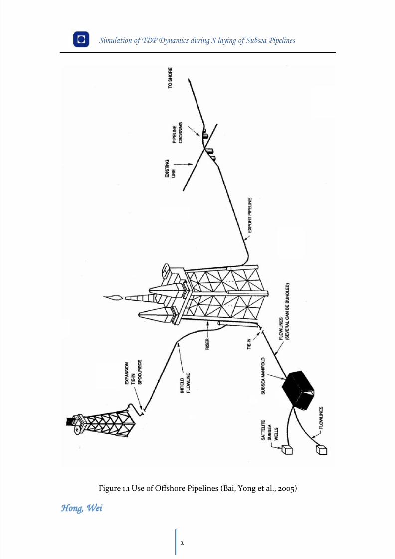
Figure 1.1 Use of Offshore Pipelines 2
Figure 2.1 S-lay Method for Shallow to Deep pipelines 5
Figure 2.2 Typical Roller/Support for Pipeline 6
Figure 2.3 Typical Tensioner Support 7
Figure 2.4 J-lay Method for Deepwater Pipelines 8
Figure 2.5 Technip’s DP Vertical Reel Vessel Deep Blue (J-lay) 10
Figure 2.6 Bottom Tow for Pipeline Installation 12
Figure 2.7 Off-bottom Tow for Pipeline Installation 14
Figure 2.8 Mid-depth Tow for Pipeline Installation 15
Figure 2.9 Surface Tow for Pipeline installation 16
Figure 3.1 External Forces Per Unit Length 21
Figure 4.1 Domain of Applicability of the Various Theories 25
Figure 4.2 Definition of Wave Direction 28
Figure 4.3 CL in shear and shear-free flow for 103<Re<30×104 34
Figure 5.1 Euler-Cauchy Incrementing 37
Figure 5.2 Newton-Raphson Algorithm 38
8/11/2019 Cañerías Offshore Instalación
http://slidepdf.com/reader/full/canerias-offshore-instalacion 8/157
Simulation of TDP Dynamics during S-laying of Subsea Pipelines
vii
Figure 5.3 Newton-Raphson Iteration 39
Figure 5.4 Modified Newton-Raphson Methods 39
Figure 5.5 Combined Incremental and Iterative Solution Procedures 42
Figure 5.6 Representation of Line Search 43
Figure 5.7 Geometric Representations of Different Control Strategies of
Nonlinear Solution Methods for Single d.o.f. 44
Figure 5.8 Schematic Representation of the Arc-Length Technique 45
Figure 5.9 Arc-Length Control Methods 46
Figure 6.1 SIMLA System Architecture 51
Figure 6.2 S-lay Model 51
Figure 6.3 The S-Lay Model in XPOST 62
Figure 7.1 Element Displacement Element 10213 End 1 Dof2 with 0 deg Wave
Direction 69
Figure 7.2 Element Displacement Element 10213 End 1 Dof2 for 45 deg Wave
Direction 69
Figure 7.3 Element Displacement Element 10213 End 1 Dof2 for 90 deg Wave
Direction 70
Figure 7.4 Element Force Element 10213 End 1 Dof 2 for 0 deg Wave Direction
70
Figure 7.5 Element Force Element 10213 End 1 Dof 2 for 45 deg Wave Direction
71
Figure 7.6 Element Force Element 10213 End 1 Dof 2 for 90 deg Wave Direction
71
Figure 7.7 Element Force Element 10213 End 1 Dof 3 for 0 deg Wave Direction
72
8/11/2019 Cañerías Offshore Instalación
http://slidepdf.com/reader/full/canerias-offshore-instalacion 9/157
Simulation of TDP Dynamics during S-laying of Subsea Pipelines
viii
Figure 7.8 Element Force Element 10213 End 1 Dof 3 for 45 deg Wave Direction
72
Figure 7.9 Element Force Element 10213 End 1 Dof 3 for 90 deg Wave Direction 73
Figure 7.10 Element Displacement Element 10212 End 1 Dof2 with 0 deg Wave
Direction 73
Figure 7.11 Element Displacement Element 10212 End 1 Dof2 for 45 deg Wave
Direction 74
Figure 7.12 Element Displacement Element 10212 End 1 Dof2 for 90 deg Wave
Direction 74
Figure 7.13 Element Force Element 10212 End 1 Dof2 for 0 deg Wave Direction
75
Figure 7.14 Element Force Element 10212 End 1 Dof2 for 0 deg Wave Direction
75
Figure 7.15 Element Force Element 10212 End 1 Dof2 for 90 deg Wave Direction
76
Figure 7.16 Element Force Element 10212 End 1 Dof3 for 0 deg Wave Direction
76
Figure 7.17 Element Force Element 10212 End 1 Dof3 for 45 deg Wave Direction
77
Figure 7.18 Element Force Element 10212 End 1 Dof3 for 90 deg Wave Direction
77
Figure 7.19 Element Displacement Element 10211 End 1 Dof2 for Hs=1m 78
Figure 7.20 Element Displacement Element 10211 End 1 Dof2 for Hs=2m 78
Figure 7.21 Element Displacement Element 10211 End 1 Dof2 for Hs=3m 79
Figure 7.22 Element Displacement Element 10211 End 1 Dof2 for Hs=4m 79
Figure 7.23 Element Force Element 10211 End 1 Dof2 for Hs=1m 80
8/11/2019 Cañerías Offshore Instalación
http://slidepdf.com/reader/full/canerias-offshore-instalacion 10/157
Simulation of TDP Dynamics during S-laying of Subsea Pipelines
ix
Figure 7.24 Element Force Element 10211 End 1 Dof2 for Hs=2m 80
Figure 7.25 Element Force Element 10211 End 1 Dof2 for Hs=3m 81
Figure 7.26 Element Force Element 10211 End 1 Dof2 for Hs=4m 81
Figure 7.27 Element Force Element 10211 End 1 Dof3 for Hs=1m 82
Figure 7.28 Element Force Element 10211 End 1 Dof3 for Hs=2m 82
Figure 7.29 Element Force Element 10211 End 1 Dof3 for Hs=3m 83
Figure 7.30 Element Force Element 10211 End 1 Dof3 for Hs=4m 83
Figure 7.31 Element Displacement Element 10210 End 1 Dof2 for Hs=1m 84
Figure 7.32 Element Displacement Element 10210 End 1 Dof2 for Hs=2m 84
Figure 7.33 Element Displacement Element 10210 End 1 Dof2 for Hs=3m 85
Figure 7.34 Element Displacement Element 10210 End 1 Dof2 for Hs=4m 85
Figure 7.35 Element Force Element 10210 End 1 Dof2 for Hs=1m 86
Figure 7.36 Element Force Element 10210 End 1 Dof2 for Hs=2m 86
Figure 7.37 Element Force Element 10210 End 1 Dof2 for Hs=3m 87
Figure 7.38 Element Force Element 10210 End 1 Dof2 for Hs=4m 87
Figure 7.39 Element Force Element 10210 End 1 Dof3 for Hs=1m 88
Figure 7.40 Element Force Element 10210 End 1 Dof3 for Hs=2m 88
Figure 7.41 Element Force Element 10210 End 1 Dof3 for Hs=3m 89
Figure 7.42 Element Force Element 10210 End 1 Dof3 for Hs=4m 89
Figure 7.43 Element Force Element 10213 End 1 Dof3 for Hs=1m 90
Figure 7.44 Element Force Element 10213 End 1 Dof3 for Hs=2m 90
8/11/2019 Cañerías Offshore Instalación
http://slidepdf.com/reader/full/canerias-offshore-instalacion 11/157
Simulation of TDP Dynamics during S-laying of Subsea Pipelines
x
Figure 7.45 Element Force Element 10213 End 1 Dof3 for Hs=3m 91
Figure 7.46 Element Force Element 10213 End 1 Dof3 for Hs=4m 91
Figure 7.47 Element Force Element 10213 End 1 Dof2 for Hs=1m 92
Figure 7.48 Element Force Element 10213 End 1 Dof2 for Hs=2m 92
Figure 7.49 Element Force Element 10213 End 1 Dof2 for Hs=3m 93
Figure 7.50 Element Force Element 10213 End 1 Dof2 for Hs=4m 93
Figure 7.51 Element Force Element 10213 End 1 Dof2 for Hs=1m 94
Figure 7.52 Element Displacement Element 10213 End 1 Dof2 for Hs=2m 94
Figure 7.53 Element Displacement Element 10213 End 1 Dof2 for Hs=3m 95
Figure 7.54 Element Displacement Element 10213 End 1 Dof2 for Hs=4m 95
8/11/2019 Cañerías Offshore Instalación
http://slidepdf.com/reader/full/canerias-offshore-instalacion 12/157
Simulation of TDP Dynamics during S-laying of Subsea Pipelines
Hong Wei
1
Chapter 1 Introduction
The first pipeline was built in the United States in 1859 to transport crude oil
(Wolbert, 1952). During the past one and a half decade, it has been proven to
the most economical means of large scale overland transportation for crude oil,natural gas and other products. The pipeline has been used extensively for
many purposes as illustrated in Figure 1.1:
Export (transportation) pipelines;
Flowlines to transfer product from a platform to export lines;
Water injection or chemical injection flowlines;
Flowlines to transfer product between platforms, subsea manifolds and
satellite wells;
Pipeline bundles.
8/11/2019 Cañerías Offshore Instalación
http://slidepdf.com/reader/full/canerias-offshore-instalacion 13/157
8/11/2019 Cañerías Offshore Instalación
http://slidepdf.com/reader/full/canerias-offshore-instalacion 14/157
Simulation of TDP Dynamics during S-laying of Subsea Pipelines
Hong Wei
3
During installation of subsea pipelines, the penetration of the pipe prior to
operation has a tendency of being larger than the predicted values. This may
have large consequences with respect to intervention work and cost impact. It
is therefore of interest to investigate whether this behavior can be explained bythe dynamics at the touch down point (TDP) induced by vessel 1st order
motions from waves.
The thesis work therefore focuses on dynamic simulation of pipelines using the
computer code SIMLA and puts special emphasis on investigating the work
done by the pipe onto the soil at TDP as the installation process goes on.
SIMLA is MARINTEK’s newly developed computer tool for analysis of offshore
pipelines in deep waters and rough environments.
The thesis may be divided into two major parts. The first part describes the
background theory material. Brief introduction is given to the offshore pipeline
installation technology in which S-lay, J-lay, reel lay method, and tow or pull
method are described briefly. During pipeline installation and the subsequent
operation phase, the contact of the pipeline and seabed also known as the
pipe-soil interaction should be studied. Pipeline resting on the seabed is
subjected to hydrodynamic forces arising from the wave and current. The
response of the pipeline is nonlinear due to nonlinear hydrodynamic forces and
nonlinear interaction between the pipe and soil. Nonlinear finite elementmethod is applied to perform the computing the dynamic response of the
pipeline.
The second part focuses on the dynamic simulation of pipelines using the
computer code SIMLA. A dynamic analysis model for 32 inch pipeline at
200-300 water depth is established. The influence of various parameters viz.
wave height, wave period and wave direction are investigated in this thesis. 4
sea states and 3 wave propagation directions are considered. Thus there are
total 12 combinations of sea state and wave propagation direction. The
simulations of the 12 cased are performed respectively. Then we try to
investigate the TDP dynamics as a function of sea state. Special emphasis is put
on the dynamic pipe-soil interaction force and displacement as a function of
time.
8/11/2019 Cañerías Offshore Instalación
http://slidepdf.com/reader/full/canerias-offshore-instalacion 15/157
Simulation of TDP Dynamics during S-laying of Subsea Pipelines
Hong Wei
4
Chapter 2 Offshore Pipeline Installation
Technology
2.1 Introduction
To keep up with the trend of the discovery of oil and gas fields in deeper and
deeper water depth up to 3000 m, the pipeline installation technology has
beegreatly improved in the past twenty years. There are several methods for
pipeline installation as follows:
a) S-lay method
b)
J-lay method
c) Reel lay method
d) Tow or pull method including bottom tow, off-bottom tow, mid depth tow,
surface tow.
Among those above, S-lay, J-lay, reel lay are the most common methods in
practice. S-laying is used in a range of water depth from shallow to deep water,
while J-laying and reeling from intermediate to deep water. Tow or pullmethods can be used from shallow water to deep water. Herein, the shallow
water depth ranges from shore to 500 feet. The range for intermediate water
depth is from 500 feet to 1000 feet. And the deep water is water depth greater
than 1000 feet. What’s more, different vessel types will be adapted depending
on the installation methods used and site characteristics (water depth, weather
etc).
S-lay/J-lay semisubmersibles;
8/11/2019 Cañerías Offshore Instalación
http://slidepdf.com/reader/full/canerias-offshore-instalacion 16/157
Simulation of TDP Dynamics during S-laying of Subsea Pipelines
Hong Wei
5
S-lay/J-lay ships;
Reel ships;
Tow or pull vessels.
Most of the material in this chapter is collected from (Boyun Guo et al., 2005)
and (Gilbert Gedeon, 2001).
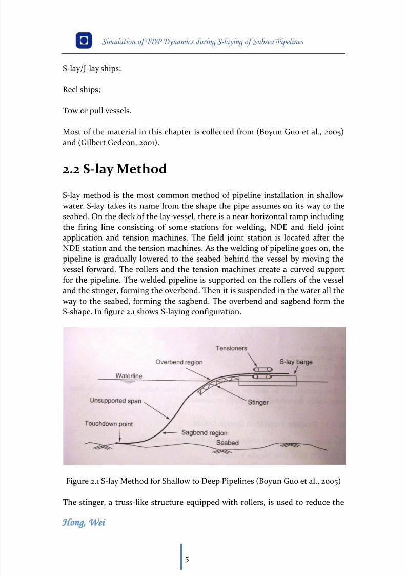
2.2 S-lay Method
S-lay method is the most common method of pipeline installation in shallow
water. S-lay takes its name from the shape the pipe assumes on its way to the
seabed. On the deck of the lay-vessel, there is a near horizontal ramp including
the firing line consisting of some stations for welding, NDE and field joint
application and tension machines. The field joint station is located after the
NDE station and the tension machines. As the welding of pipeline goes on, the
pipeline is gradually lowered to the seabed behind the vessel by moving the
vessel forward. The rollers and the tension machines create a curved support
for the pipeline. The welded pipeline is supported on the rollers of the vessel
and the stinger, forming the overbend. Then it is suspended in the water all the
way to the seabed, forming the sagbend. The overbend and sagbend form theS-shape. In figure 2.1 shows S-laying configuration.
Figure 2.1 S-lay Method for Shallow to Deep Pipelines (Boyun Guo et al., 2005)
The stinger, a truss-like structure equipped with rollers, is used to reduce the
8/11/2019 Cañerías Offshore Instalación
http://slidepdf.com/reader/full/canerias-offshore-instalacion 17/157
Simulation of TDP Dynamics during S-laying of Subsea Pipelines
Hong Wei
6
curvature and therefore the bending stress of the pipe as it leaves the vessel.
The stinger is normally made up of more than one section. Through moving the
sections relative to the vessel and each other, different assemblies can be made.
The position of the rollers relative to the section they belong to can be changedtoo. Thus, a vessel can be configured for a number of different radiuses of
curvature. The stinger radius controls the overbend curvature. And the vessel
has an upper and lower limit of the departure angle at which the pipeline
departs from the stinger due to the limitations for both minimum and
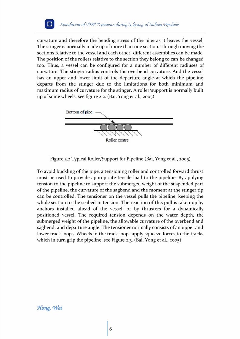
maximum radius of curvature for the stinger. A roller/support is normally built
up of some wheels, see figure 2.2. (Bai, Yong et al., 2005)
Figure 2.2 Typical Roller/Support for Pipeline (Bai, Yong et al., 2005)
To avoid buckling of the pipe, a tensioning roller and controlled forward thrust
must be used to provide appropriate tensile load to the pipeline. By applyingtension to the pipeline to support the submerged weight of the suspended part
of the pipeline, the curvature of the sagbend and the moment at the stinger tip
can be controlled. The tensioner on the vessel pulls the pipeline, keeping the
whole section to the seabed in tension. The reaction of this pull is taken up by
anchors installed ahead of the vessel, or by thrusters for a dynamically
positioned vessel. The required tension depends on the water depth, the
submerged weight of the pipeline, the allowable curvature of the overbend and
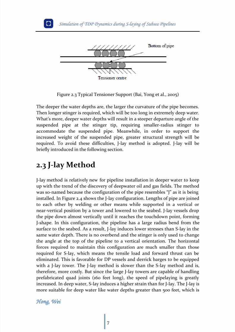
sagbend, and departure angle. The tensioner normally consists of an upper and
lower track loops. Wheels in the track loops apply squeeze forces to the tracks
which in turn grip the pipeline, see Figure 2.3. (Bai, Yong et al., 2005)
8/11/2019 Cañerías Offshore Instalación
http://slidepdf.com/reader/full/canerias-offshore-instalacion 18/157
Simulation of TDP Dynamics during S-laying of Subsea Pipelines
Hong Wei
7
Figure 2.3 Typical Tensioner Support (Bai, Yong et al., 2005)
The deeper the water depths are, the larger the curvature of the pipe becomes.
Then longer stinger is required, which will be too long in extremely deep water.
What’s more, deeper water depths will result in a steeper departure angle of the
suspended pipe at the stinger tip, requiring smaller-radius stinger to
accommodate the suspended pipe. Meanwhile, in order to support the
increased weight of the suspended pipe, greater structural strength will be
required. To avoid these difficulties, J-lay method is adopted. J-lay will be
briefly introduced in the following section.
2.3 J-lay Method
J-lay method is relatively new for pipeline installation in deeper water to keep
up with the trend of the discovery of deepwater oil and gas fields. The method
was so-named because the configuration of the pipe resembles “J” as it is being
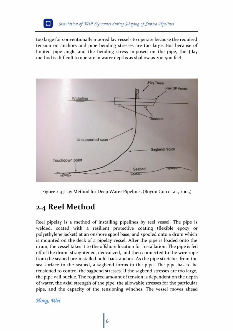
installed. In Figure 2.4 shows the J-lay configuration. Lengths of pipe are joined
to each other by welding or other means while supported in a vertical or
near-vertical position by a tower and lowered to the seabed. J-lay vessels drop
the pipe down almost vertically until it reaches the touchdown point, forming
J-shape. In this configuration, the pipeline has a large radius bend from the
surface to the seabed. As a result, J-lay induces lower stresses than S-lay in the
same water depth. There is no overbend and the stinger is only used to change
the angle at the top of the pipeline to a vertical orientation. The horizontal
forces required to maintain this configuration are much smaller than those
required for S-lay, which means the tensile load and forward thrust can be
eliminated. This is favorable for DP vessels and derrick barges to be equipped
with a J-lay tower. The J-lay method is slower than the S-lay method and is,
therefore, more costly. But since the large J-lay towers are capable of handling
prefabricated quad joints (160 feet long), the speed of pipelaying is greatly
increased. In deep water, S-lay induces a higher strain than for J-lay. The J-lay is
more suitable for deep water like water depths greater than 500 feet, which is
8/11/2019 Cañerías Offshore Instalación
http://slidepdf.com/reader/full/canerias-offshore-instalacion 19/157
Simulation of TDP Dynamics during S-laying of Subsea Pipelines
Hong Wei
8
too large for conventionally moored lay vessels to operate because the required
tension on anchors and pipe bending stresses are too large. But because of
limited pipe angle and the bending stress imposed on the pipe, the J-lay
method is difficult to operate in water depths as shallow as 200-500 feet.
Figure 2.4 J-lay Method for Deep Water Pipelines (Boyun Guo et al., 2005)
2.4 Reel Method
Reel pipelay is a method of installing pipelines by reel vessel. The pipe is
welded, coated with a resilient protective coating (flexible epoxy or
polyethylene jacket) at an onshore spool base, and spooled onto a drum which
is mounted on the deck of a pipelay vessel. After the pipe is loaded onto the
drum, the vessel takes it to the offshore location for installation. The pipe is fed
off of the drum, straightened, deovalized, and then connected to the wire rope
from the seabed pre-installed hold-back anchor. As the pipe stretches from the
sea surface to the seabed, a sagbend forms in the pipe. The pipe has to be
tensioned to control the sagbend stresses. If the sagbend stresses are too large,
the pipe will buckle. The required amount of tension is dependent on the depth
of water, the axial strength of the pipe, the allowable stresses for the particular
pipe, and the capacity of the tensioning winches. The vessel moves ahead
8/11/2019 Cañerías Offshore Instalación
http://slidepdf.com/reader/full/canerias-offshore-instalacion 20/157
Simulation of TDP Dynamics during S-laying of Subsea Pipelines
Hong Wei
9
slowly usually at about one knot depending on weather conditions while it
slowly reels out the pipe. When the drum has been emptied, a pullhead
connected a wire rope is attached. The A&R wire rope from the reel vessel is
played out slowly maintaining sufficient tension in the pipe until the pipe restson the seabed. A buoy is attached to the end of the A&R cable. Then the reel
vessel returns to the spool base to replenish the reel or take on a fully loaded
new drum. On returning to the site, it pulls the end of the pipe using the A&R
cable, removes the pullhead, and welds it to the pipe on the drum. Then the
unreeling process goes on.
The pipe undergoes plastic deformation when it is reeled onto a drum. Thus the
pipe experiences some plastic strain. So the diameter of the pipe is restricted by
the permissible amount of strain. Usually, the maximum diameter of the pipe is
up to 18 inches. And also, due to the limited size of the drum, only short
lengths of the pipe can be laid (usually 3-15km depending on pipe diameter).
However, it is possible to install larger lines if more drums of pipe are available.
The reeled pipeline can be installed in either S-lay method or J-lay method,
depending on the design of the reel vessel and the water depths. Reel vessels
are divided into two classes-horizontal reel and vertical reel.
Horizontal reel vessels lay pipelines in shallow to intermediate water depths.
S-lay method is adopted. The axis of rotation is vertical with respect to thebarge deck. Both anchors and DP can be used for station-keeping of the
horizontal reel vessels.
Vertical reel vessels lay is versatile. It can lay pipes from shallow water depths
to very deep water depths. This method minimizes bending stresses in the
overbend region. If the drum is bottom-loaded, the pipe is fed off horizontally
making it well suited for shallow water. For deepwater pipelaying, the drum is
top-loaded and the pipe is discharged vertically after it is straightened. For
intermediate water depths, the angle of entry can be adjusted according to the
engineering calculations and judgments. For deepwater, J-lay method is used.
And since bending stresses are minimized by the vertical reel method, no
stinger is needed. Only DP is used for station-keeping of the vertical reel
vessels.
There are many advantages of the reel method. First, since no on-board
welding is needed, the method speeds up the pipeline installation process. The
speed of pipelaying with reel method can be up to 10 times faster than
conventional pipelaying, which means pipelaying is allowed during a fairly
short weather window and the conventional construction season can be
8/11/2019 Cañerías Offshore Instalación
http://slidepdf.com/reader/full/canerias-offshore-instalacion 21/157
Simulation of TDP Dynamics during S-laying of Subsea Pipelines
Hong Wei
10
extended by several months.
Most of the welding, x-raying inspection, corrosion coating and testing are
accomplished on shore. Thus the labor cost is greatly reduced since labor coston shore is generally lower than that offshore. Moreover, the processes such as
welding, x-raying inspection and so on are performed under controlled
conditions onshore. In this way, the quality of the pipeline construction is
greatly enhanced.
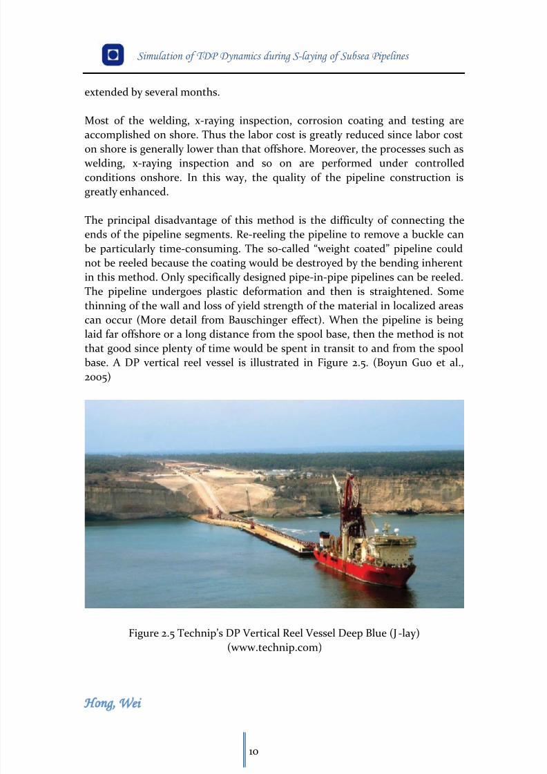
The principal disadvantage of this method is the difficulty of connecting the
ends of the pipeline segments. Re-reeling the pipeline to remove a buckle can
be particularly time-consuming. The so-called “weight coated” pipeline could
not be reeled because the coating would be destroyed by the bending inherent
in this method. Only specifically designed pipe-in-pipe pipelines can be reeled.
The pipeline undergoes plastic deformation and then is straightened. Some
thinning of the wall and loss of yield strength of the material in localized areas
can occur (More detail from Bauschinger effect). When the pipeline is being
laid far offshore or a long distance from the spool base, then the method is not
that good since plenty of time would be spent in transit to and from the spool
base. A DP vertical reel vessel is illustrated in Figure 2.5. (Boyun Guo et al.,
2005)
Figure 2.5 Technip’s DP Vertical Reel Vessel Deep Blue (J-lay)
(www.technip.com)
8/11/2019 Cañerías Offshore Instalación
http://slidepdf.com/reader/full/canerias-offshore-instalacion 22/157
Simulation of TDP Dynamics during S-laying of Subsea Pipelines
Hong Wei
11
2.5 Tow Methods
Compared to the previous three methods, tow method is less commonly used.The fabrication and assembly of the pipeline, that is welding, inspection,
joint-coating, and anode installation, are all performed onshore. The
fabrication cost is much lower than that offshore. Due to the limited size of the
fabrication yard, this method is normally applied to short lines, usually less
than 7km. It is particularly well-suited to pipe-in-pipe flowline assemblies,
which can be fabricated more efficiently onshore and which contain thermal
insulation in the annular space between the inner and outer pipes.
The pipeline can be made up in two ways – perpendicular and parallel to the
shoreline.
In the perpendicular launch method, a long enough land to accommodate the
longest section of the fabricated pipeline has to be leased. A rail system is
installed from the shore end right into the water. First, all the sections that
make up the pipeline are fabricated and tested. And then, the first section of
the pipeline is lifted by side booms and placed on the rollers of the rail system.
The section is attached to the cable from the tow vessel and is pulled into the
water, leaving sufficient length onshore to make a welded tie-in to the next
section. Then section by section, the whole pipeline is fabricated and pulledinto the water. To keep the pipeline under control, a hold-back winch is used
during pulling.
In the parallel launch method, the length of the land along the shore should
normally be equal to the total length of the pipeline. Compared to
perpendicular method, no rail system is needed. After all the sections of the
pipeline are welded and tested, the sections are strung along the shoreline.
Then all the sections are welded together to make up the pipeline. After that,
the pipeline is moved into the water using side-bottom tractors and crawler
cranes for the end structures. The front end is attached to the tow vessel, while
the rear end is attached to a hold-back anchor. The pipeline is gradually moved
laterally into the water by the winches in the anchored tow vessel. At the same
time, the curvature of the pipeline is monitored all the time. When the whole
length of the pipeline and its end structures are in a straight line, the tow vessel
starts to tow the pipeline along the predetermined tow route.
When the pipeline is to be towed into deepwater, pressurized nitrogen can be
introduced to the pipeline in order to prevent collapse or buckling under
external hydrostatic pressure.
8/11/2019 Cañerías Offshore Instalación
http://slidepdf.com/reader/full/canerias-offshore-instalacion 23/157
Simulation of TDP Dynamics during S-laying of Subsea Pipelines
Hong Wei
12
There are four variations of the tow method: bottom tow, off-bottom tow,
mid-depth tow, and surface tow. (Boyun Guo et al., 2005)
2.5.1 Bottom tow
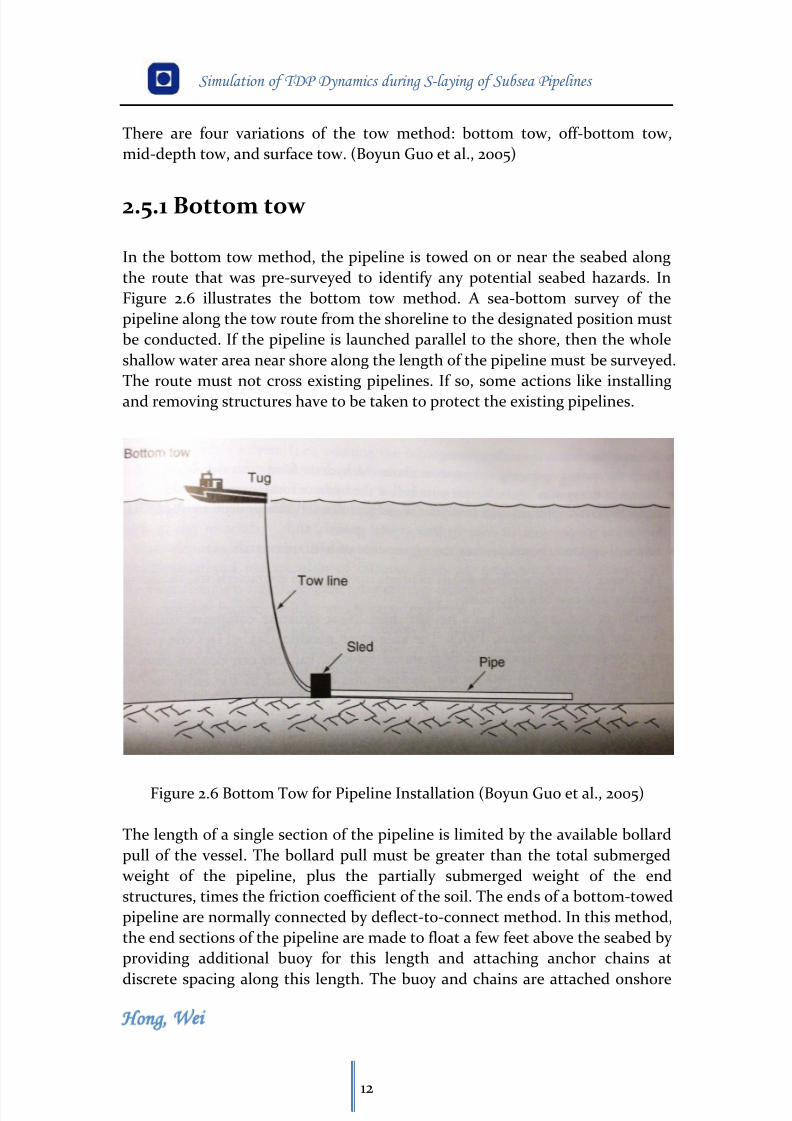
In the bottom tow method, the pipeline is towed on or near the seabed along
the route that was pre-surveyed to identify any potential seabed hazards. In
Figure 2.6 illustrates the bottom tow method. A sea-bottom survey of the
pipeline along the tow route from the shoreline to the designated position must
be conducted. If the pipeline is launched parallel to the shore, then the whole
shallow water area near shore along the length of the pipeline must be surveyed.
The route must not cross existing pipelines. If so, some actions like installing
and removing structures have to be taken to protect the existing pipelines.
Figure 2.6 Bottom Tow for Pipeline Installation (Boyun Guo et al., 2005)
The length of a single section of the pipeline is limited by the available bollard
pull of the vessel. The bollard pull must be greater than the total submerged
weight of the pipeline, plus the partially submerged weight of the end
structures, times the friction coefficient of the soil. The ends of a bottom-towed
pipeline are normally connected by deflect-to-connect method. In this method,
the end sections of the pipeline are made to float a few feet above the seabed by
providing additional buoy for this length and attaching anchor chains at
discrete spacing along this length. The buoy and chains are attached onshore
8/11/2019 Cañerías Offshore Instalación
http://slidepdf.com/reader/full/canerias-offshore-instalacion 24/157
8/11/2019 Cañerías Offshore Instalación
http://slidepdf.com/reader/full/canerias-offshore-instalacion 25/157
Simulation of TDP Dynamics during S-laying of Subsea Pipelines
Hong Wei
14
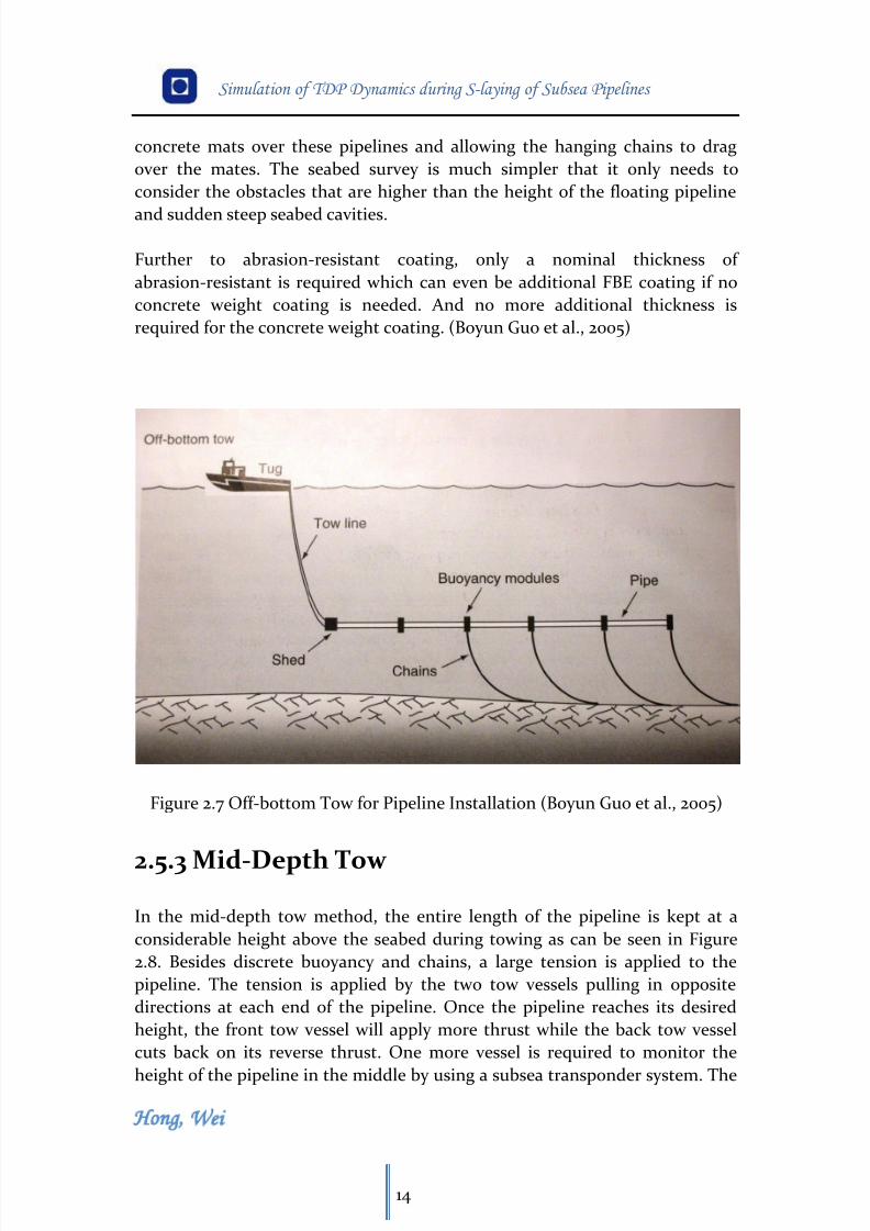
concrete mats over these pipelines and allowing the hanging chains to drag
over the mates. The seabed survey is much simpler that it only needs to
consider the obstacles that are higher than the height of the floating pipeline
and sudden steep seabed cavities.
Further to abrasion-resistant coating, only a nominal thickness of
abrasion-resistant is required which can even be additional FBE coating if no
concrete weight coating is needed. And no more additional thickness is
required for the concrete weight coating. (Boyun Guo et al., 2005)
Figure 2.7 Off-bottom Tow for Pipeline Installation (Boyun Guo et al., 2005)
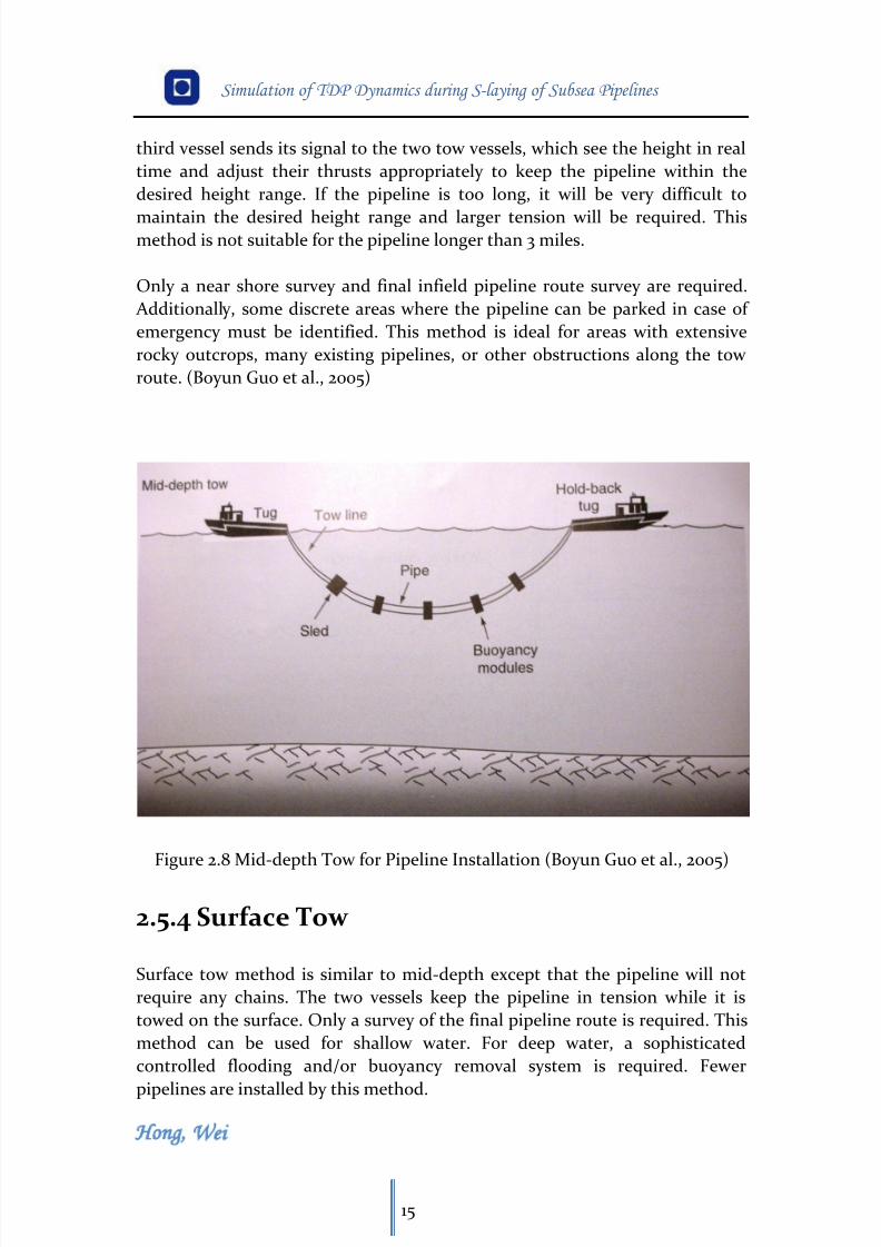
2.5.3 Mid-Depth Tow
In the mid-depth tow method, the entire length of the pipeline is kept at a
considerable height above the seabed during towing as can be seen in Figure
2.8. Besides discrete buoyancy and chains, a large tension is applied to the
pipeline. The tension is applied by the two tow vessels pulling in opposite
directions at each end of the pipeline. Once the pipeline reaches its desired
height, the front tow vessel will apply more thrust while the back tow vessel
cuts back on its reverse thrust. One more vessel is required to monitor the
height of the pipeline in the middle by using a subsea transponder system. The
8/11/2019 Cañerías Offshore Instalación
http://slidepdf.com/reader/full/canerias-offshore-instalacion 26/157
8/11/2019 Cañerías Offshore Instalación
http://slidepdf.com/reader/full/canerias-offshore-instalacion 27/157
Simulation of TDP Dynamics during S-laying of Subsea Pipelines
Hong Wei
16
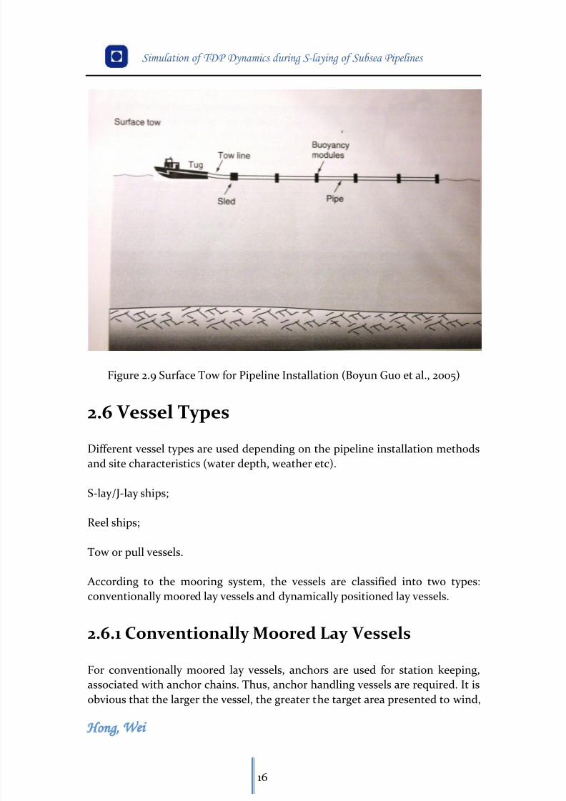
Figure 2.9 Surface Tow for Pipeline Installation (Boyun Guo et al., 2005)
2.6 Vessel TypesDifferent vessel types are used depending on the pipeline installation methods
and site characteristics (water depth, weather etc).
S-lay/J-lay ships;
Reel ships;
Tow or pull vessels.
According to the mooring system, the vessels are classified into two types:
conventionally moored lay vessels and dynamically positioned lay vessels.
2.6.1 Conventionally Moored Lay Vessels
For conventionally moored lay vessels, anchors are used for station keeping,
associated with anchor chains. Thus, anchor handling vessels are required. It is
obvious that the larger the vessel, the greater the target area presented to wind,
8/11/2019 Cañerías Offshore Instalación
http://slidepdf.com/reader/full/canerias-offshore-instalacion 28/157
Simulation of TDP Dynamics during S-laying of Subsea Pipelines
Hong Wei
17
wave, and current forces and the heavier the vessel are. As a result, a higher
holding is required for the mooring system. The rated holding capacity of an
anchor system is a function of the weight and size of the anchor and the tensile
strength of the chain that secures the anchor to the vessel. The pipelayingmethods have little effect on the required number of anchors. The number of
anchors used for a conventionally moored lay vessel is 8-12 anchors, depending
on lay barge size.
The limitation of conventionally moored lay vessel is the anchor handling
vessel. The deeper the operating water depths, the higher the requirements for
the anchor handling vessels. Compared to monohull vessels, semisubmersibles
have better sea keeping abilities. They are more suitable to operate in the tough
weather conditions. But for shallow water, the cost effectiveness of
semisubmersibles is lower than the monohull vessel. (Gilbert Gedeon, 2001)
2.6.2 Dynamically Positioned Lay Vessels
For dynamically positioned lay vessels, the location or position of the vessel is
maintained by the vessels’ special station-keeping system, which, instead of or
in addition to the conventional propeller-rudder system at the stern, employs a
system of hull-mounted thrusters near the bow, at mid-ship, and at the stern.
In the station-keeping mode, these thrusters, which have the capability torotate 360o in a horizontal plane, are controlled by a shipboard computer
system that usually interfaces with a satellite-based geographic positioning
system.
Considering the cost effectiveness, the minimum water depth at which
dynamically positioned lay vessels are used is no less than 600 ft. But for reel
vessels, sometimes it is used in shallow water. (Gilbert Gedeon, 2001)
8/11/2019 Cañerías Offshore Instalación
http://slidepdf.com/reader/full/canerias-offshore-instalacion 29/157
Simulation of TDP Dynamics during S-laying of Subsea Pipelines
Hong Wei
18
Chapter 3 Pipe-Soil Interaction
3.1 Introduction
During the installation and subsequent operation phase, the pipeline is laid to
rest on the seabed. Obviously, the mechanical properties of the seabed will
affect the pipeline stability significantly. Geotechnical investigation is needed
to get the information about the seabed.The pipe-soil soil model consists of
seabed stiffness and equivalent friction definition to represent the soil
resistance o movement of the pipe. It is important to predict the soil contact
pressure, equivalent and soil stiffness accurately. Ole and Torseten (2008)
developed a generalized true 3D elastoplastic spring element based on an
anisotropic hardening/degradation model for sliding for pipe-soil interaction
analysis. The model complies with finite element format allowing it to be
directly implemented in a simple way.
3.2 Geotechnical Survey
Geotechnical investigations are performed to obtain information on the
physical properties of soil and rock in a site. In subsea geotechnical engineering,
seabed materials are considered a two-phase material composed of rock or
mineral particles and water. The mechanical properties of the seabed will affectthe pipeline stability significantly. Thus, geotechnical survey data provide
important information on seabed conditions that can affect both pipeline
mechanical design and operations. Seafloor bathymetry would affect pipeline
routing, alignment, and spanning. Pipeline should be routed away from any
seafloor obstructions and hazards. Spanning analysis should be conducted,
based upon geotechnical survey data, to identify any locations where spans will
be longer than allowable span lengths. Understanding the soil mechanical
properties will help the design of subsea pipelines.
8/11/2019 Cañerías Offshore Instalación
http://slidepdf.com/reader/full/canerias-offshore-instalacion 30/157
Simulation of TDP Dynamics during S-laying of Subsea Pipelines
Hong Wei
19
Soil mechanical properties depend largely upon the soil components and their
fractions. There are coarse-grained components, like boulder, cobble, gravel,
and sand. The fine grained components consist mainly of silt, clay, and organic
matter (Lambe and Whitman, 1969). Boulders and cobbles are very stablecomponents. Foundations with boulders and cobbles present good stability. Silt
is unstable and, with increased water moisture, becomes a "quasi-liquid"
offering little resistance to erosion and piping. Clay is difficult to compact when
it is wet, but compacted clay is resistant to erosion. Organic matters tend to
increase the compressibility of the soil and reduce the soil stability.
Silt and clay are the major components of seabed soil down to a few feet in
depth. Thus, when pipeline is laid on the seabed, it will normally sink into the
soil. How much the pipeline will sink depends largely upon the mechanical
properties of the soil. The following parameters are normally obtained when
performing geotechnical analysis.
Water moisture content is defined as the ratio of the mass of the free water in
the soil to the mass of soil solid material. Water moisture content is normally
expressed as a percentage. Some soils can hold so much water that their water
moisture content can be more than 100%.
Absolute porosity is defined as the ratio, expressed as a percentage, of void
volume of soil to the soil bulk volume.
Absolute permeability is defined as a measure of the soil's ability to transmit
fluid. To determine the permeability of the soil, a sample is put into a pressure
device and water is conducted through the soil. The rate of water flow under a
given pressure drop is proportional to the soil permeability.
Liquid limit is determined by measuring the water moisture content and the
number of blows required to close a specific groove which was cut through a
standard brass cup filled with soil. Liquid limit indicates how much water the
soil can hold without getting into the "liquid" state.
Plastic limit is defined as the water moisture content at which a thread of soil
with 3.2-mm diameter begins to crumble. Plastic limit is the minimum water
content required for the soil to present "plastic" properties.
Plasticity index is defined as the difference between liquid limit and plastic
limit.
Liquidity index, LI, is defined as the ratio of the difference between the
8/11/2019 Cañerías Offshore Instalación
http://slidepdf.com/reader/full/canerias-offshore-instalacion 31/157
Simulation of TDP Dynamics during S-laying of Subsea Pipelines
Hong Wei
20
natural water moisture content and the plastic limit to the plasticity index.
Activity number is defined as the ratio of plasticity index to the weight
percentage of soil particles finer than 2 macros. Activity number indicates howmuch water will be attracted into soil. (Boyun Guo et al., 2005)
3.2 Pipe-Soil Interaction Model
Once in contact, the interaction between the pipeline and the soil can be
described in terms of 3 d.o.f: penetration into the seabed (normal to the
seabed), axial movements along the axis of the pipeline and lateral movement
perpendicular to the pipeline. The penetration of the pipeline into the seabed
has a great influence on the axial and lateral resistance. Many studies about the
pipe-soil interaction had been done, referring to (Lyons, 1973), (Lambrakos,
1985), (Karal, 1977), (Brennodden, et al., 1986), (Wagner et al., 1987), (Morris et
al., 1988) and (Palmer et al., 1988). These studies show that a pipeline moving
cyclically accumulates penetration, which therefore results in an increased
lateral soil resistance. H. Brennodden et al. (1985) developed an energy-based
pipe-soil interaction model to predict soil resistance to lateral motion of
untrenched pipelines based on full- scale pipe-soil interaction tests. The tests
confirm that soil resistance is strongly dependent on pipe penetration and soil
condition (shear strength of clay and relative density of sand). The total soilresistance into two terms: one is the sliding resistance force and the other is
penetration dependent soil resistance force. This method is applied for
PONDUS pipe-soil interaction model in SIMLA. The specific information refers
to Appendix A. In this section, several methods for calculating the seabed
penetration for clay as a function of the static ground pressure exist. Among
them, Verley and Lund Method (Verley and Lund, 1995) and the buoyancy
method (Håland, 1997) are briefly introduced below. Most of the material in
this section is collected from (Bai, Yong et al., 2005).
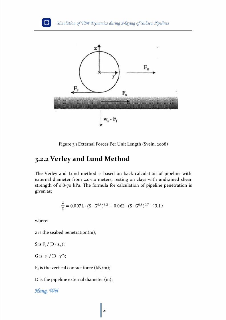
Figure 3.1 shows the positive direction of the dynamic external forces per unit
length acting on the submerged pipe.
8/11/2019 Cañerías Offshore Instalación
http://slidepdf.com/reader/full/canerias-offshore-instalacion 32/157
Simulation of TDP Dynamics during S-laying of Subsea Pipelines
Hong Wei
21
Figure 3.1 External Forces Per Unit Length (Svein, 2008)
3.2.2 Verley and Lund Method
The Verley and Lund method is based on back calculation of pipeline with
external diameter from 2.0-1.0 meters, resting on clays with undrained shear
strength of 0.8-70 kPa. The formula for calculation of pipeline penetration is
given as:
z
D= 0.0071 ⋅ (S ⋅ G0.3)3.2 + 0.062 ⋅ (S ⋅ G0.3)0.7 (3.1)
where:
z is the seabed penetration(m);
S is Fc (D ⋅ su) ;
G is su (D ⋅ γ′) ;
Fc is the vertical contact force (kN/m);
D is the pipeline external diameter (m);
8/11/2019 Cañerías Offshore Instalación
http://slidepdf.com/reader/full/canerias-offshore-instalacion 33/157
Simulation of TDP Dynamics during S-laying of Subsea Pipelines
Hong Wei
22
su is the undrained shear strength (kPa);
γ' is the submerged soil density (kN/m2).
The Verley and Lund formulation is based on curve fitting to data with
S⋅D0.3<2.5. For larger values the method overestimates penetration. An
alternative formulation which is valid for values of S⋅D0.3, is given by:
z
D= 0.09 ⋅ (S ⋅ G0.3)(3.2)
3.2.2 Buoyancy method
The method is only used with pipeline resting on very soft clays. The buoyancy
method assumes that the soil has no strength and behaves like a heavy liquid.
The penetration is estimated by demanding that the soil-induced buoyancy of
the pipeline is equal to the vertical contact forces.
B = 2 ⋅ D ⋅ z − z2 (3.3)
As = (z 6B ) ⋅ (3 ⋅ z2 + 4 ⋅ B2)(3.4)
O = As ⋅ L ⋅ γ′ (3.5)
where:
B is the width of pipeline in contact with soil;
A s is the penetrated cross sectional area of pipe;
O is the buoyancy.
The equivalent friction is mainly based on coulomb friction for sand, cohesion
for clay, or combination of the two, the soil density and the contact pressure
between the pipe and soil. For the friction model, in the case that the pipeline
doesn’t penetrate into the seabed much, a pure Coulomb friction model can be
appropriate. When the pipeline penetrates into the seabed, the forces required
moving the pipeline laterally become larger than the forces needed to move it
8/11/2019 Cañerías Offshore Instalación
http://slidepdf.com/reader/full/canerias-offshore-instalacion 34/157
Simulation of TDP Dynamics during S-laying of Subsea Pipelines
Hong Wei
23
in the longitudinal direction. The reason for this effect is passive lateral soil
resistance is produced when a wedge of soil resists the pipe’s motion. An
anisotropic friction model that defines different friction coefficients in the
lateral and longitudinal directions of the pipeline is suitable. In SIMLA, thefriction is modeled based on the same principles as applied for material
plasticity (Levold, 1990).Two major ingredients are included a friction surface
and a slip rule. More information is referred to Appendix A. (Bai, Yong et al.,
2005)
The breakout force is the maximum force needed to move the pipe from its
stable position on the seabed. This force can be significantly higher than the
force needed to maintain the movement after breakout due to suction and extra
force needed for the pipe to “climb” out of its depression.
(Brennodden, 1991) gives the following equations for the maximum breakout
force in the axial and lateral direction:
Axial soil resistance (kN/m):
Fa,max = 1.05 ⋅ Ac,calc ⋅ su (3.6)
Lateral soil resistance (kN/m):
Fl,max = 0.8 ⋅ (0.2 ⋅ Fc + 1.47 ⋅ su ⋅ Ac,calc D ) (3.7)
where:
Fc is the vertical contact force (kN/m);
A c,calc equals 2 ⋅ R ⋅ Acos1 − zR (m2);
z is the seabed penetration;
su is the undrained shear strength (kPa).
8/11/2019 Cañerías Offshore Instalación
http://slidepdf.com/reader/full/canerias-offshore-instalacion 35/157
8/11/2019 Cañerías Offshore Instalación
http://slidepdf.com/reader/full/canerias-offshore-instalacion 36/157
Simulation of TDP Dynamics during S-laying of Subsea Pipelines
Hong Wei
25
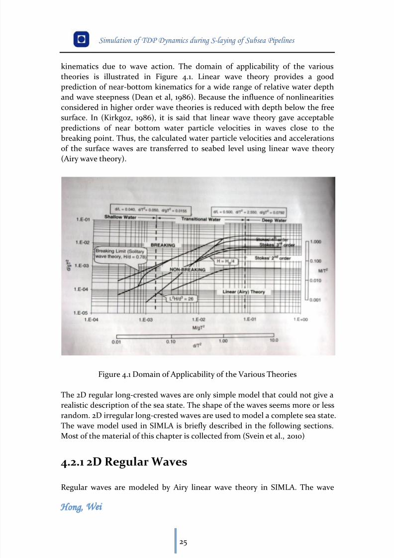
kinematics due to wave action. The domain of applicability of the various
theories is illustrated in Figure 4.1. Linear wave theory provides a good
prediction of near-bottom kinematics for a wide range of relative water depth
and wave steepness (Dean et al, 1986). Because the influence of nonlinearitiesconsidered in higher order wave theories is reduced with depth below the free
surface. In (Kirkgoz, 1986), it is said that linear wave theory gave acceptable
predictions of near bottom water particle velocities in waves close to the
breaking point. Thus, the calculated water particle velocities and accelerations
of the surface waves are transferred to seabed level using linear wave theory
(Airy wave theory).
Figure 4.1 Domain of Applicability of the Various Theories
The 2D regular long-crested waves are only simple model that could not give a
realistic description of the sea state. The shape of the waves seems more or less
random. 2D irregular long-crested waves are used to model a complete sea state.
The wave model used in SIMLA is briefly described in the following sections.
Most of the material of this chapter is collected from (Svein et al., 2010)
4.2.1 2D Regular Waves
Regular waves are modeled by Airy linear wave theory in SIMLA. The wave
8/11/2019 Cañerías Offshore Instalación
http://slidepdf.com/reader/full/canerias-offshore-instalacion 37/157
Simulation of TDP Dynamics during S-laying of Subsea Pipelines
Hong Wei
26
potential φ0 for a regular wave according to Airy’s theory can be expressed as
follows:
φ0 = ζagω C1cos(−ωt + kXcosβ + kYsinβ +ψφ) (4.1)
where ζa is the wave amplitude, g is the acceleration of gravity, k is the wave
number, β is the direction of wave propagation(where β=0 corresponds to wave
propagation along the positive X-axis) and ψφ is a phase angle lag.
C1 is given by:
C1 =coshk(Z + D)
coshkD (4.2)
where D is the water depth.
In deep water, C1 can be approximated by
C1 ≈ ekZ (4.3)
Then, the particle velocities and accelerations in the undisturbed field areobtained:
υx = −ζaωcosβC2sinψ (4.4)
υy = −ζaωcosβC2sinψ (4.5)
υz =
−ζa
ωC3cos
ψ (4.6)
ax = ζaω2cosβC2cosψ (4.7)
ay = ζaω2sinβC2cosψ (4.8)
az = ζaω2C3sinψ (4.9)
where

8/11/2019 Cañerías Offshore Instalación
http://slidepdf.com/reader/full/canerias-offshore-instalacion 38/157
Simulation of TDP Dynamics during S-laying of Subsea Pipelines
Hong Wei
27
ψ = −ωt + kXcosβ + kYsinβ + ψφ (4.10)
According to the approximation we make for the deep water, we can get:
C1 = C2 = C3 = ekZ (4.11)
In the case of finite water depth, we can get:
C1 =coshk(Z + D)
coshkD (4.12)
C2 =coshk(Z + D)
sinhkD (4.13)
C3 =sinhk(Z + D)
sinhkD (4.14)
The surface elevation is expressed as:
ζ = −ζasinψ = ζasin(ωt − kXcosβ − kYsinβ + ϕ) (4.15)
where ϕ=-ψ, phase angle.
The linearized dynamic pressure is given by:
pd = ρgζaC1sinψ (4.16)
4.2.2 2D Irregular Waves
The irregular wave formulation is based on the use of wave spectra. Significant
wave height, peak period etc define the characteristics of the sea state. In
SIMLA, an irregular sea state is described as a sum of two wave spectra: a wind
sea contribution and a swell contribution:
Sζ,TOT β,ω = Sζ,1ωϕ1(β − β1) + Sζ,2ωϕ2(β − β2) (4.17)
where Sζ,1 and Sζ,2 describe the frequency distribution of the wind sea and swell,
respectively. Spectra included in SIMLA are Pierson-Moscowitz and Jonswap.
8/11/2019 Cañerías Offshore Instalación
http://slidepdf.com/reader/full/canerias-offshore-instalacion 39/157
Simulation of TDP Dynamics during S-laying of Subsea Pipelines
Hong Wei
28
ϕ1 and ϕ2 describe the directionality of the waves. So far only unidirectional
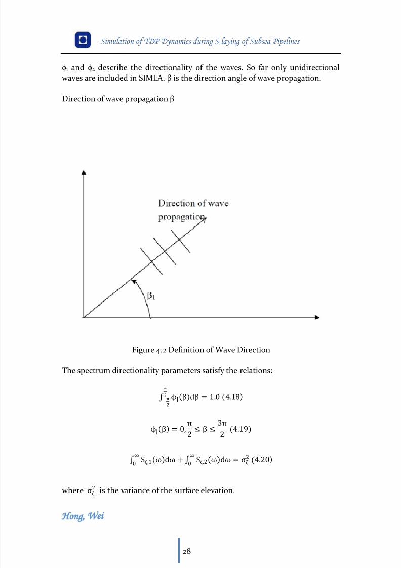
waves are included in SIMLA. β is the direction angle of wave propagation.
Direction of wave propagation β
Figure 4.2 Definition of Wave Direction
The spectrum directionality parameters satisfy the relations:
ϕjβdβπ2
−π2 = 1.0 (4.18)
ϕjβ = 0,π2≤ β ≤ 3π
2 (4.19)
Sζ,1ωdω∞0
+ Sζ,2ωdω∞0
= ςζ2 (4.20)
where
ςζ2 is the variance of the surface elevation.
8/11/2019 Cañerías Offshore Instalación
http://slidepdf.com/reader/full/canerias-offshore-instalacion 40/157
Simulation of TDP Dynamics during S-laying of Subsea Pipelines
Hong Wei
29
In order to generate time series of surface elevation, water particle velocities
and accelerations, the short crested irregular sea is discretized into a set of
harmonic components. In complex notation, the surface elevation is expressed
by:
Zζ = Zjk
Nωk=1
Nβj=1
= Ajk ei(ωk t+ϕjk
p+ϕjk )
Nωk=1
Nβj=1
(4.21)
Ajk = Zjk = 2Sζ(βi ,ωk )ΔβΔω (4.22)
argZjk = ωk t + ϕjk
p
+ϕjk (4.23)
The random phase angles, ϕ jk are sampled from a uniform distributions over–ϕ,ϕ. The position dependent phase angle is:
ϕjk
p= −k k Xcosβj − k k Ysinβj (4.24)
The surface elevation can be expressed as:
ζt Im Zζ = Re Zζe−π
2 = Ajk sin ωk t + ϕjk
p+ ϕjk Nω
k=1
Nβj=1
(4.25)
The velocity and acceleration components are derived from the surface
elevation components.
Z jk = iωk Ζjk , Ζ jk = −ωk 2
Ζjk (4.26)
4.2.3 Steady Currents
When a steady current also exists, the effects of the bottom boundary layer may
be accounted for. And the mean current velocity over the pipe diameter may be
applied in the analysis. According to (DNV, 1998), this has been included in the
finite element model by assuming a logarithmic mean velocity profile.
8/11/2019 Cañerías Offshore Instalación
http://slidepdf.com/reader/full/canerias-offshore-instalacion 41/157
Simulation of TDP Dynamics during S-laying of Subsea Pipelines
Hong Wei
30
UczD =U(zr)
ln(zr z0 )e
D+ 1 lne + D z0 − e
D ln e
z0
− 1 (4.27)
where
U(zr) is the current velocity at reference measurement height;
zr is reference measurement height (usually 3m);
zD is height to mid pipe (from seabed);
z0 is the bottom roughness parameter;
e is the gap between the pipeline and the seabed;
D is the total external diameter of pipe (including any coating).
Then the total velocity is obtained by adding the velocities from waves and
currents together.
4.3 Hydrodynamic Forces
Hydrodynamic forces arise from water particle velocity and acceleration. These
forces can be fluctuating (caused by waves) or constant (caused by steady
currents) and will result in a dynamic load pattern on the pipeline. Drag, inertia,
and lift forces are of interest when analyzing the behavior of a submerged
pipeline subjected to wave and/or current loading. Because of the dynamic
nature of waves, the pipeline response when subjected to this type of loading
may be investigated in a dynamic analysis. 2D regular or random long-crested
waves and the 3D regular or random short-crested waves may be included in
the finite element model to supply the wave kinematics in a dynamic analysis.
Most of the material is collected from (Bai, Yong et al., 2005).
4.3.1 Hydrodynamic Drag Forces
The drag force, FD due to water particle velocities is given by:
FD =1
2
ρCDD(U + V)2 (4.28)
8/11/2019 Cañerías Offshore Instalación
http://slidepdf.com/reader/full/canerias-offshore-instalacion 42/157
Simulation of TDP Dynamics during S-laying of Subsea Pipelines
Hong Wei
31
where:
FD is the drag force per unit length;
ρ is the mass density of seawater;
CD is the drag coefficient;
D is the outside diameter of pipeline (including the coatings);
U is the water particle velocity due to waves;
V is the current velocity.
4.3.2 Hydrodynamic Inertia Force
The inertia force, Fi due to water particle acceleration is given by:
Fi = ρ CM
π4
D2a (4.29)
where:
Fi is the inertia force per length;
ρ is the mass density of seawater;
CM is the inertia coefficient;
D is the outside diameter of pipeline (including the coatings);
a is the water particle acceleration due to waves.
The total force is given by Morison’s equation.
The drag and inertia coefficients are given by:
CD = CDRe , KC,α, e D , k D , AZ D (4.30)
8/11/2019 Cañerías Offshore Instalación
http://slidepdf.com/reader/full/canerias-offshore-instalacion 43/157
8/11/2019 Cañerías Offshore Instalación
http://slidepdf.com/reader/full/canerias-offshore-instalacion 44/157
8/11/2019 Cañerías Offshore Instalación
http://slidepdf.com/reader/full/canerias-offshore-instalacion 45/157
Simulation of TDP Dynamics during S-laying of Subsea Pipelines
Hong Wei
34
FL =1
2ρDCLνn
2 (4.37)
where:
CL is the lift coefficient for pipe on a surface;
νn is the transverse water particle velocity (perpendicular to the direction of the
lift force);
ρ is the density of seawater;
D is the total external diameter of pipe.
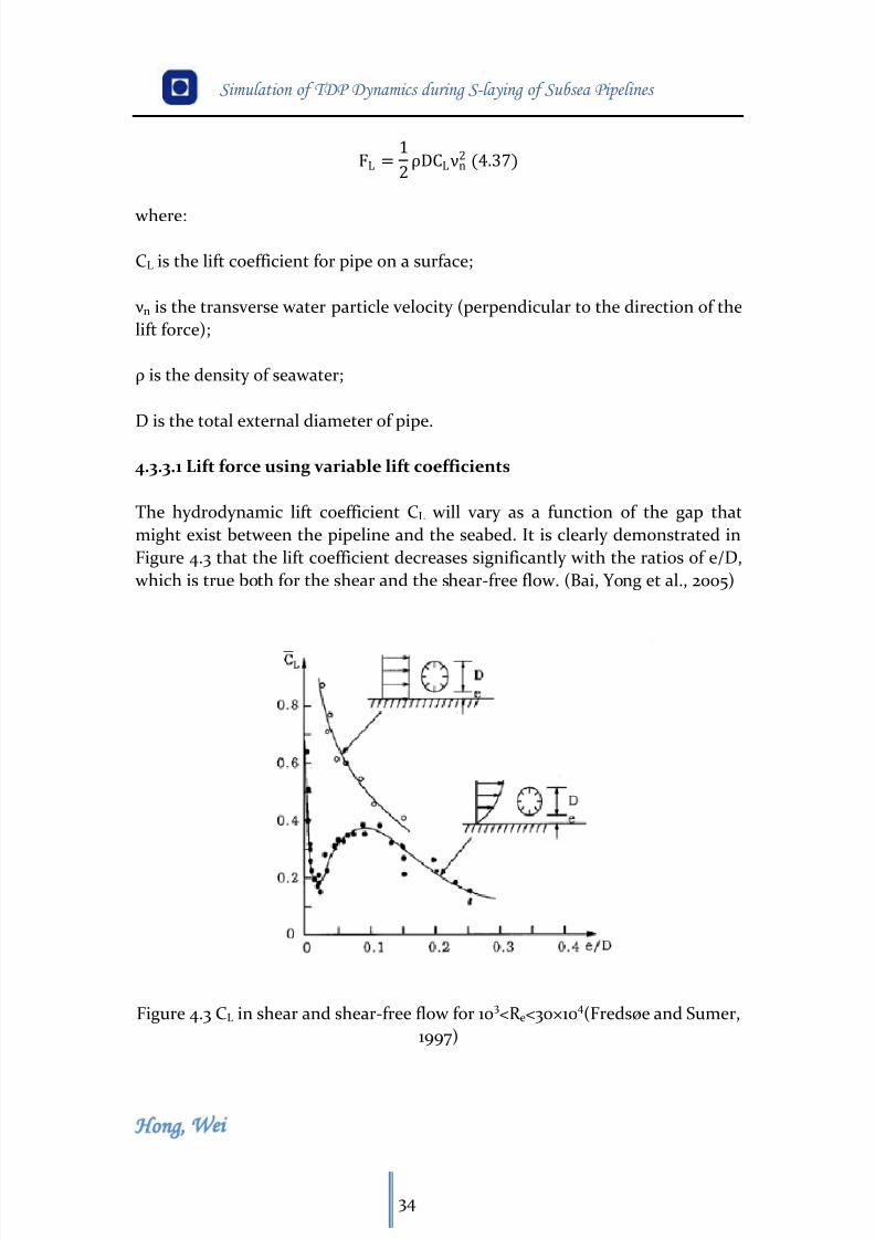
4.3.3.1 Lift force using variable lift coefficients
The hydrodynamic lift coefficient CL will vary as a function of the gap that
might exist between the pipeline and the seabed. It is clearly demonstrated in
Figure 4.3 that the lift coefficient decreases significantly with the ratios of e/D,
which is true both for the shear and the shear-free flow. (Bai, Yong et al., 2005)
Figure 4.3 CL in shear and shear-free flow for 103<R e<30×104(Fredsøe and Sumer,
1997)
8/11/2019 Cañerías Offshore Instalación
http://slidepdf.com/reader/full/canerias-offshore-instalacion 46/157
8/11/2019 Cañerías Offshore Instalación
http://slidepdf.com/reader/full/canerias-offshore-instalacion 47/157
Simulation of TDP Dynamics during S-laying of Subsea Pipelines
Hong Wei
36
5.2 Total Lagrangian and the Updated
Lagrangian (UL) formulationsThe difference between the Total Lagrangian and Updated Lagrangian
formations is the choice of reference configuration. In a TL formulation, all
static and kinematic variables are referred to the initial (C0) configuration,
while in the UL formulation these are referred to the last obtained equilibrium
configuration, i.e. the current (Cn) configuration.
Several variations of the TL and UL formulations have been developed to
improve the computational efficiency. The basic idea is to separate the rigid
body motion from the local or relative deformation of the element. This is done
by attaching a local coordinate system to the element and letting it
continuously translate and rotate with the element during deformation. The
nonlinearities arising from large displacements can be separated from the
nonlinearities within the element. Several terms have been introduced to label
various formulations. Examples of names are Co-rotational Formulation and
Co-rotated Ghost Reference Formulation.
In SIMLA, the present work has been based on the Co-Rotational Formulation
referring all quantities to the C0 configuration. In the Co-rotationalformulation, the last obtained reference configuration is adequately described
by the current strains and the equation of incremental stiffness is obtained by
making use of principle of virtual work and study the virtual work in an
infinitesimal increment. (Svein, 2008)
5.3 Solution Techniques
Various techniques for directly solving the nonlinear problems are available.
The following methods are briefly described.
Methods for static analysis
a) Incremental or stepwise procedures (e.g. Euler-Cauchy method)
b) Iterative procedures (e.g. Newton-Raphson)
c) Combined methods (Incremental and iterative methods are combined)
8/11/2019 Cañerías Offshore Instalación
http://slidepdf.com/reader/full/canerias-offshore-instalacion 48/157
Simulation of TDP Dynamics during S-laying of Subsea Pipelines
Hong Wei
37
d) Methods based on dynamic analysis (Explicit methods)
5.3.1 Incremental MethodsIncremental methods provide a solution of the nonlinear problem by a stepwise
application of the external loading. For each step, the displacement increment
is solved. The total displacement is obtained by adding all the displacement
increments. The incremental stiffness matrix is calculated based on the known
displacement and stress condition before a new load increment is applied. The
method is also called Euler-Cauchy method.
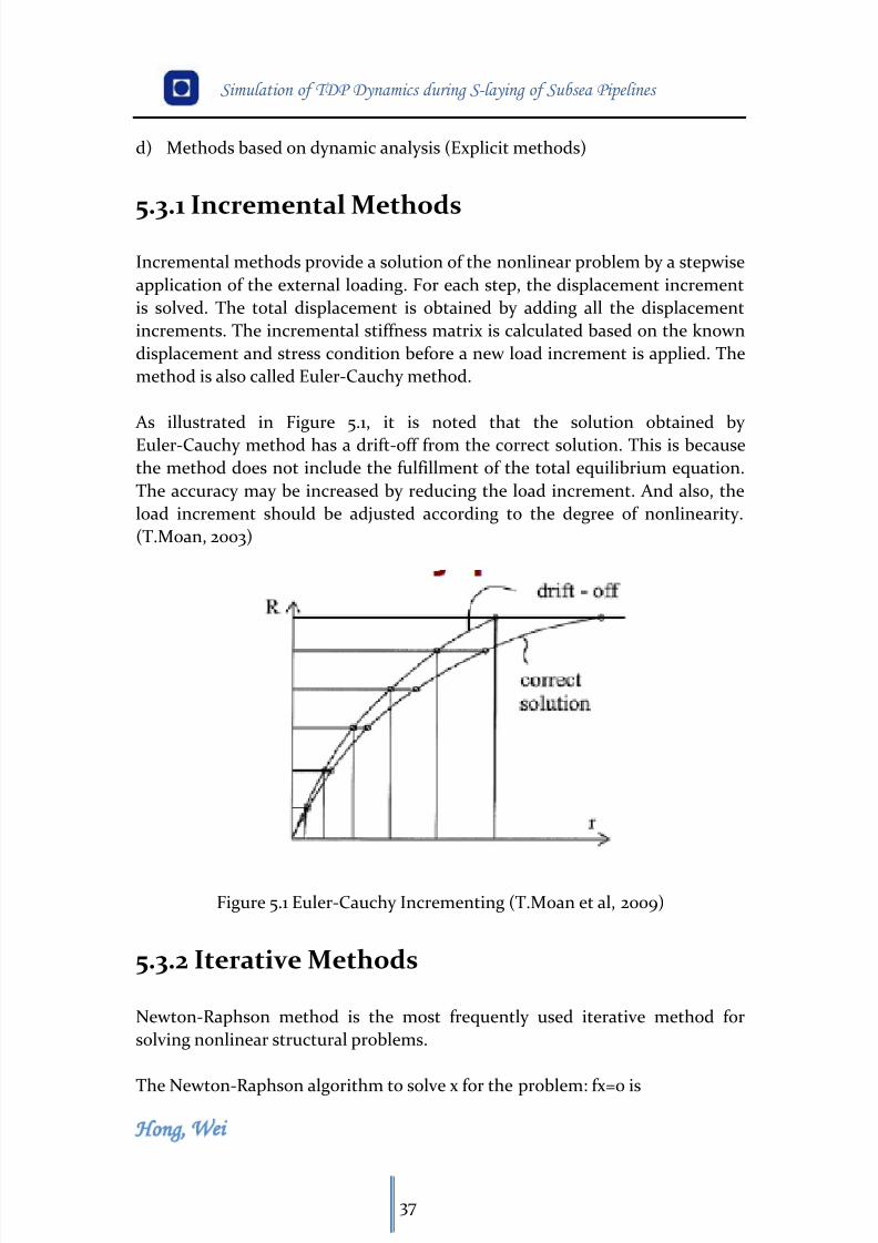
As illustrated in Figure 5.1, it is noted that the solution obtained by
Euler-Cauchy method has a drift-off from the correct solution. This is because
the method does not include the fulfillment of the total equilibrium equation.
The accuracy may be increased by reducing the load increment. And also, the
load increment should be adjusted according to the degree of nonlinearity.
(T.Moan, 2003)
Figure 5.1 Euler-Cauchy Incrementing (T.Moan et al, 2009)
5.3.2 Iterative Methods
Newton-Raphson method is the most frequently used iterative method for
solving nonlinear structural problems.
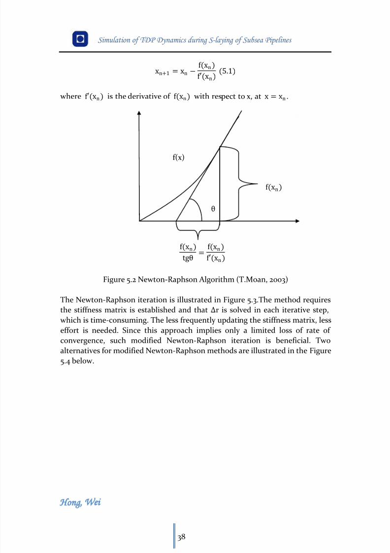
The Newton-Raphson algorithm to solve x for the problem: fx=0 is
8/11/2019 Cañerías Offshore Instalación
http://slidepdf.com/reader/full/canerias-offshore-instalacion 49/157
Simulation of TDP Dynamics during S-laying of Subsea Pipelines
Hong Wei
38
xn+1 = xn − f(xn )f′(xn) (5.1)
where f′(xn ) is the derivative of f(xn) with respect to x, at x = xn .
Figure 5.2 Newton-Raphson Algorithm (T.Moan, 2003)
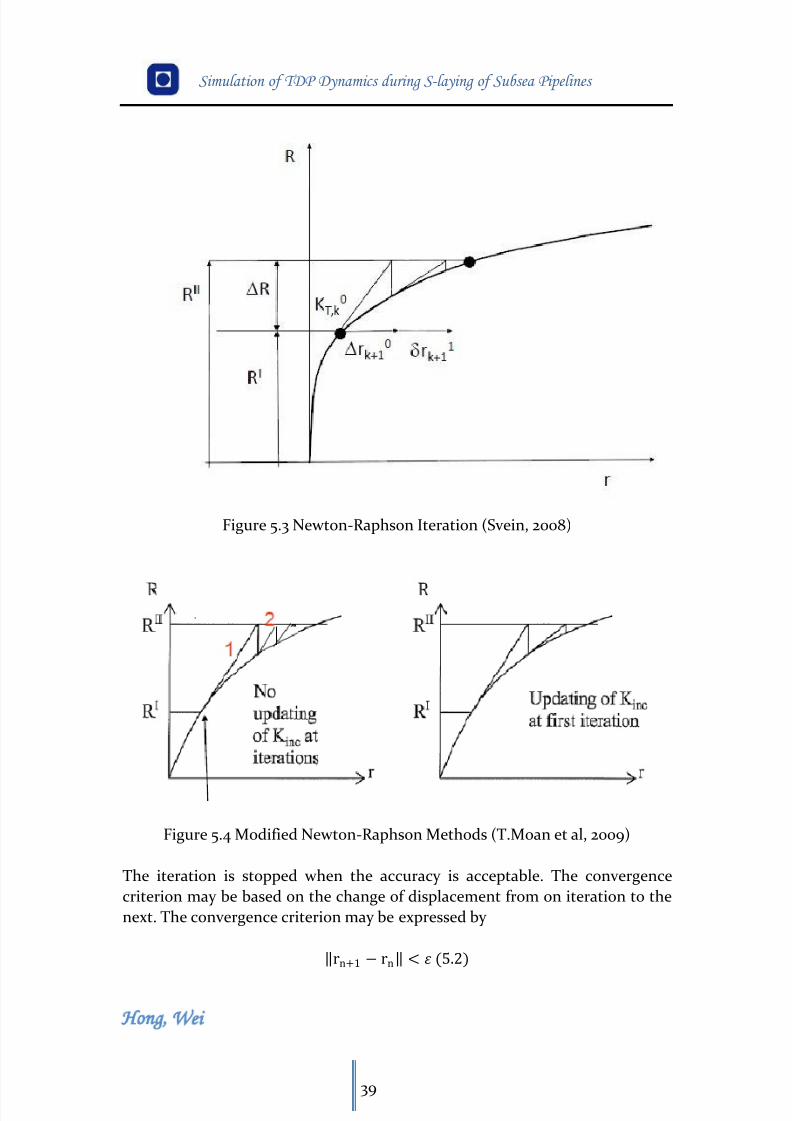
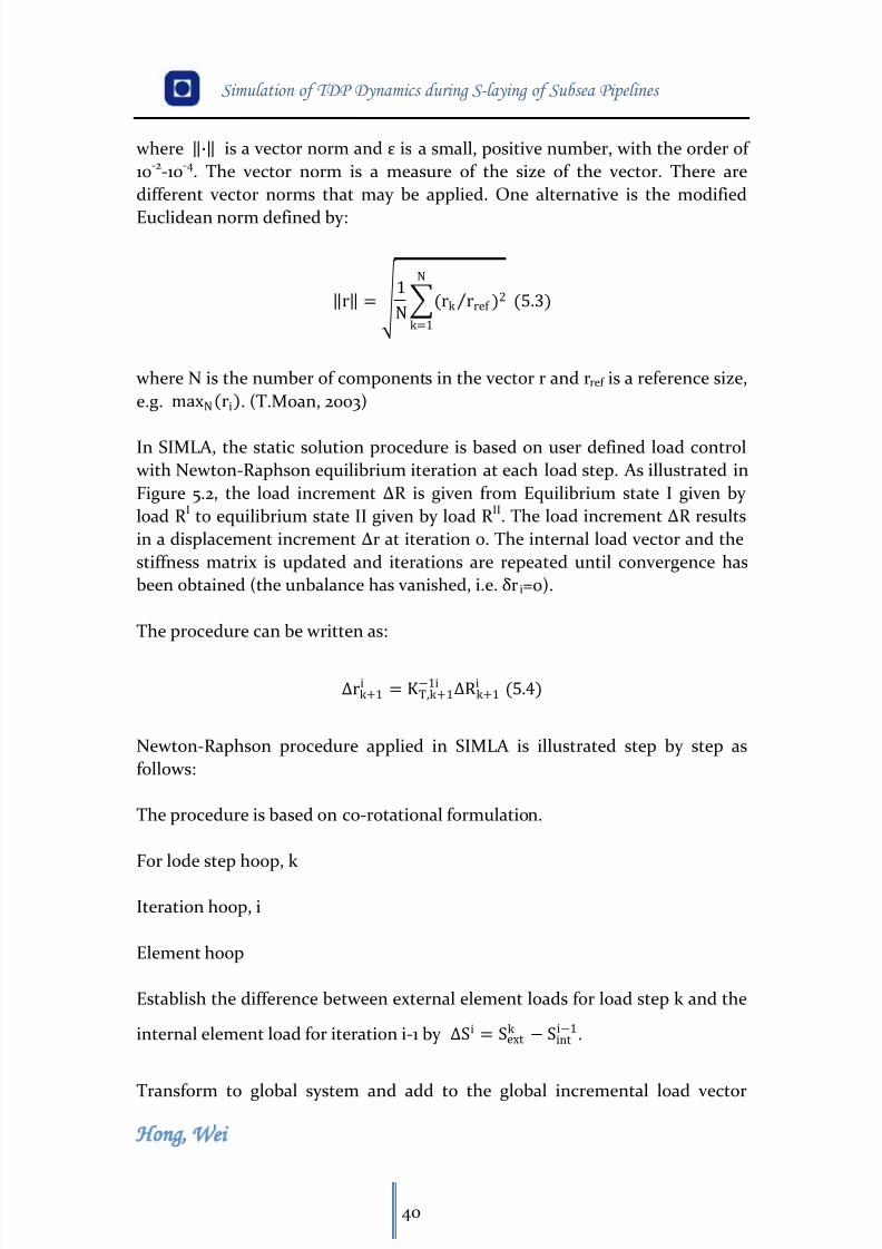
The Newton-Raphson iteration is illustrated in Figure 5.3.The method requires
the stiffness matrix is established and that ∆r is solved in each iterative step,
which is time-consuming. The less frequently updating the stiffness matrix, less
effort is needed. Since this approach implies only a limited loss of rate of
convergence, such modified Newton-Raphson iteration is beneficial. Two
alternatives for modified Newton-Raphson methods are illustrated in the Figure
5.4 below.
θ
f(xn)
tgθ =f(xn )f′(xn )
f(x)
f(xn)
8/11/2019 Cañerías Offshore Instalación
http://slidepdf.com/reader/full/canerias-offshore-instalacion 50/157
8/11/2019 Cañerías Offshore Instalación
http://slidepdf.com/reader/full/canerias-offshore-instalacion 51/157
Simulation of TDP Dynamics during S-laying of Subsea Pipelines
Hong Wei
40
where ∙ is a vector norm and ε is a small, positive number, with the order of
10-2-10-4. The vector norm is a measure of the size of the vector. There are
different vector norms that may be applied. One alternative is the modified
Euclidean norm defined by:
r = 1N(rk rref )2
N
k=1
(5.3)
where N is the number of components in the vector r and rref is a reference size,
e.g. maxN
ri
. (T.Moan, 2003)
In SIMLA, the static solution procedure is based on user defined load control
with Newton-Raphson equilibrium iteration at each load step. As illustrated in
Figure 5.2, the load increment ∆R is given from Equilibrium state I given by
load R I to equilibrium state II given by load R II. The load increment ∆R results
in a displacement increment ∆r at iteration 0. The internal load vector and the
stiffness matrix is updated and iterations are repeated until convergence has
been obtained (the unbalance has vanished, i.e. δri=0).
The procedure can be written as:
∆rk+1i = KT,k+1
−1i ∆Rk+1i (5.4)
Newton-Raphson procedure applied in SIMLA is illustrated step by step as
follows:
The procedure is based on co-rotational formulation.
For lode step hoop, k
Iteration hoop, i
Element hoop
Establish the difference between external element loads for load step k and the
internal element load for iteration i-1 by ∆Si = Sext k − Sint
i−1.
Transform to global system and add to the global incremental load vector
8/11/2019 Cañerías Offshore Instalación
http://slidepdf.com/reader/full/canerias-offshore-instalacion 52/157
Simulation of TDP Dynamics during S-laying of Subsea Pipelines
Hong Wei
41
∆Ri = ∆Ri + TT∆Si.
Establish the tangential element material stiffness matrix by numerical
integration k TMi .
Establish the element initial stress stiffness matrix (based on the current axial
force) k TSi .
Transform to global system and add to global tangential stiffness matrix
KTi = KT
i + TTk TMi + k TS
i T.
End element loop
Adjust global incremental load vector for nodal loads and prescribed
displacements, and adjust stiffness matrix for boundary conditions constrains.
Solve equation system ∆Ri = Rext k − Rint
i−1 = KTi ∆ri.
Update coordinates and nodal transformations matrices.
Element hoop
Update the element deformations vi = vi−1 + T∆ri.
Update the element stresses by evaluating each integration point.
Determine the element forces Sivi.End element loop
Calculate convergence parameters such as:
Displacement norm=∆ri2 / ri2
Force norm=∆Ri2 /Ri2
Energy norm=
∆Ri
∆ri /
Riri
8/11/2019 Cañerías Offshore Instalación
http://slidepdf.com/reader/full/canerias-offshore-instalacion 53/157
Simulation of TDP Dynamics during S-laying of Subsea Pipelines
Hong Wei
42
If the convergence criteria are satisfied, go to next load step.
If the convergence criteria are not satisfied, perform new iteration.
End iteration loop, i
End load loop step, k (T.Moan et al, 2009)
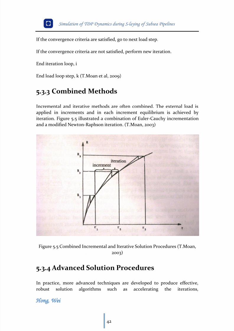
5.3.3 Combined Methods
Incremental and iterative methods are often combined. The external load is
applied in increments and in each increment equilibrium is achieved by
iteration. Figure 5.5 illustrated a combination of Euler-Cauchy incrementation
and a modified Newton-Raphson iteration. (T.Moan, 2003)
Figure 5.5 Combined Incremental and Iterative Solution Procedures (T.Moan,
2003)
5.3.4 Advanced Solution Procedures
In practice, more advanced techniques are developed to produce effective,
robust solution algorithms such as accelerating the iterations,
8/11/2019 Cañerías Offshore Instalación
http://slidepdf.com/reader/full/canerias-offshore-instalacion 54/157
Simulation of TDP Dynamics during S-laying of Subsea Pipelines
Hong Wei
43
load/displacement incrementation strategies to allow passing limit, tangent
and bifurcation points based on incremental (predictor) and iterative (corrector)
techniques and so on.
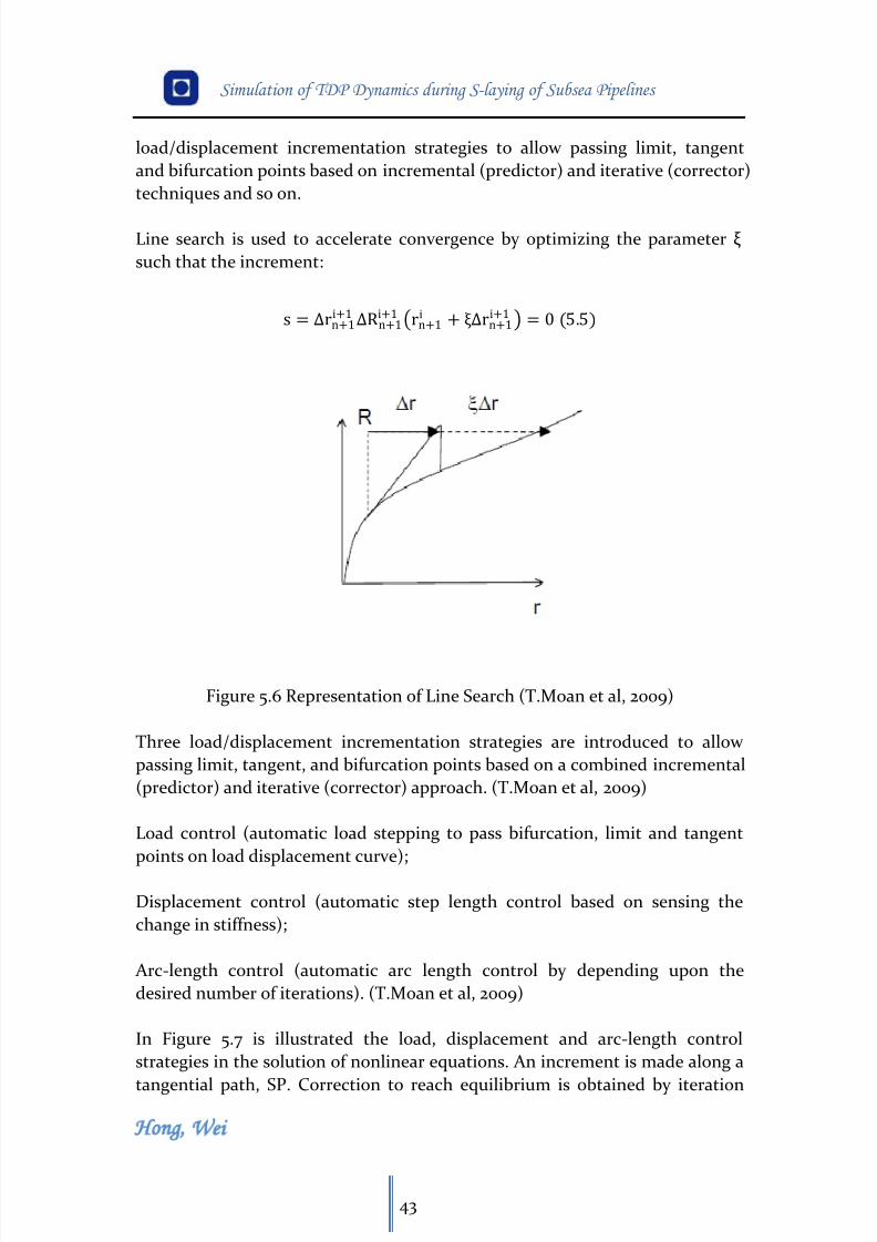
Line search is used to accelerate convergence by optimizing the parameter ξ
such that the increment:
s = Δrn+1i+1 ΔRn+1
i+1 rn+1i + ξΔrn+1
i+1 = 0 (5.5)
Figure 5.6 Representation of Line Search (T.Moan et al, 2009)
Three load/displacement incrementation strategies are introduced to allow
passing limit, tangent, and bifurcation points based on a combined incremental
(predictor) and iterative (corrector) approach. (T.Moan et al, 2009)
Load control (automatic load stepping to pass bifurcation, limit and tangent
points on load displacement curve);
Displacement control (automatic step length control based on sensing the
change in stiffness);
Arc-length control (automatic arc length control by depending upon the
desired number of iterations). (T.Moan et al, 2009)
In Figure 5.7 is illustrated the load, displacement and arc-length control
strategies in the solution of nonlinear equations. An increment is made along a
tangential path, SP. Correction to reach equilibrium is obtained by iteration
8/11/2019 Cañerías Offshore Instalación
http://slidepdf.com/reader/full/canerias-offshore-instalacion 55/157
Simulation of TDP Dynamics during S-laying of Subsea Pipelines
Hong Wei
44
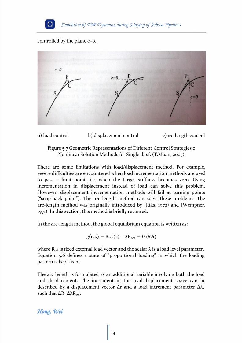
controlled by the plane c=0.
a) load control b) displacement control c)arc-length control
Figure 5.7 Geometric Representations of Different Control Strategies o
Nonlinear Solution Methods for Single d.o.f. (T.Moan, 2003)
There are some limitations with load/displacement method. For example,
severe difficulties are encountered when load incrementation methods are used
to pass a limit point, i.e. when the target stiffness becomes zero. Usingincrementation in displacement instead of load can solve this problem.
However, displacement incrementation methods will fail at turning points
(“snap-back point”). The arc-length method can solve these problems. The
arc-length method was originally introduced by (Riks, 1972) and (Wempner,
1971). In this section, this method is briefly reviewed.
In the arc-length method, the global equilibrium equation is written as:
g
r,
λ= Rint
r
− λRref = 0 (5.6)
where R ref is fixed external load vector and the scalar λ is a load level parameter.
Equation 5.6 defines a state of “proportional loading” in which the loading
pattern is kept fixed.
The arc length is formulated as an additional variable involving both the load
and displacement. The increment in the load-displacement space can be
described by a displacement vector Δr and a load increment parameter Δλ,
such that ΔR=ΔλR ref .
8/11/2019 Cañerías Offshore Instalación
http://slidepdf.com/reader/full/canerias-offshore-instalacion 56/157
Simulation of TDP Dynamics during S-laying of Subsea Pipelines
Hong Wei
45
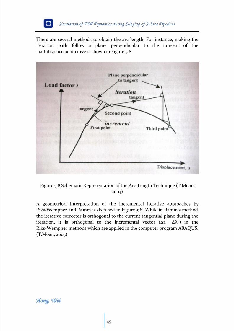
There are several methods to obtain the arc length. For instance, making the
iteration path follow a plane perpendicular to the tangent of the
load-displacement curve is shown in Figure 5.8.
Figure 5.8 Schematic Representation of the Arc-Length Technique (T.Moan,
2003)
A geometrical interpretation of the incremental iterative approaches by
Riks- Wempner and Ramm is sketched in Figure 5.8. While in Ramm’s method
the iterative corrector is orthogonal to the current tangential plane during the
iteration, it is orthogonal to the incremental vector (Δr0, Δλ 0) in the
Riks-Wempner methods which are applied in the computer program ABAQUS.
(T.Moan, 2003)
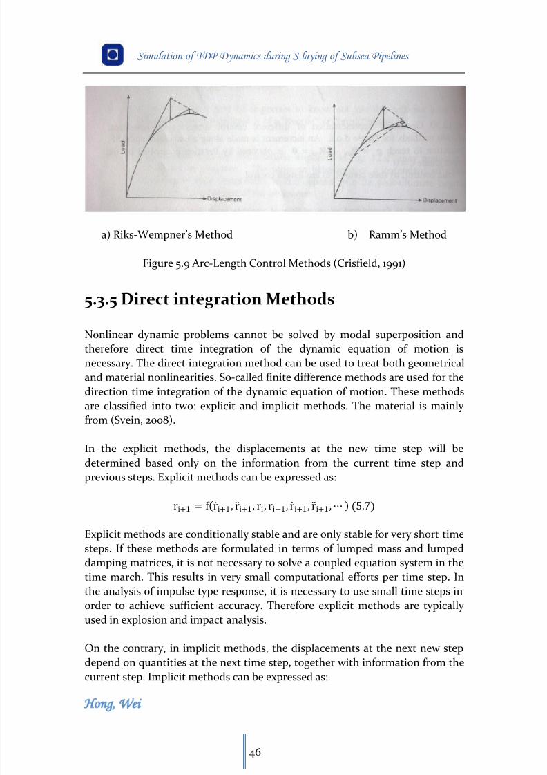
8/11/2019 Cañerías Offshore Instalación
http://slidepdf.com/reader/full/canerias-offshore-instalacion 57/157
Simulation of TDP Dynamics during S-laying of Subsea Pipelines
Hong Wei
46
a) Riks- Wempner’s Method b) Ramm’s Method
Figure 5.9 Arc-Length Control Methods (Crisfield, 1991)
5.3.5 Direct integration Methods
Nonlinear dynamic problems cannot be solved by modal superposition and
therefore direct time integration of the dynamic equation of motion is
necessary. The direct integration method can be used to treat both geometrical
and material nonlinearities. So-called finite difference methods are used for the
direction time integration of the dynamic equation of motion. These methods
are classified into two: explicit and implicit methods. The material is mainlyfrom (Svein, 2008).
In the explicit methods, the displacements at the new time step will be
determined based only on the information from the current time step and
previous steps. Explicit methods can be expressed as:
ri+1 = f r i+1 , r i+1 , ri , ri−1, r i+1 , r i+1 ,⋯ (5.7)
Explicit methods are conditionally stable and are only stable for very short time
steps. If these methods are formulated in terms of lumped mass and lumped
damping matrices, it is not necessary to solve a coupled equation system in the
time march. This results in very small computational efforts per time step. In
the analysis of impulse type response, it is necessary to use small time steps in
order to achieve sufficient accuracy. Therefore explicit methods are typically
used in explosion and impact analysis.
On the contrary, in implicit methods, the displacements at the next new step
depend on quantities at the next time step, together with information from the
current step. Implicit methods can be expressed as:
8/11/2019 Cañerías Offshore Instalación
http://slidepdf.com/reader/full/canerias-offshore-instalacion 58/157
Simulation of TDP Dynamics during S-laying of Subsea Pipelines
Hong Wei
47
rk+1 = f r k+1 , r k , r k+1 , r k , rk ,⋯ (5.8)
It is noted that the implicit methods use information at the next time step. As a
result, they will have better numerical stability than explicit methods. The various implicit methods differ in connection with how the acceleration is
assumed to vary between the time steps and at which time the equilibrium
equation is fulfilled. For instance, by assuming constant average acceleration
between the time steps, the result will be unconditionally stable, which means
that numerical stability is obtained regardless of the time step size. It is
beneficial to use such methods in case of long analysis durations. When
implicit methods are used, it is necessary to solve a coupled equation system at
every time step which will be very time-consuming. It will be uneconomical if
short time steps are unavoidable due to accuracy. In case of nonlinear systems
the guarantee of unconditional stability does not hold, but in practical cases
this is not considered to be an issue. (Langen and Sigbjørnsson, 1979)
5.3.5.1 Incremental Time Integration Scheme
In SIMLA, the HHT-α method is used in the time integration scheme. It is a
method proposed by Hilbert, Hughes and Taylor. Compared to the well known
Newmark-β method, the implicit HHT-α method will damp out high frequency
modes and at the same time retain 2nd order accuracy (Mathisen, 1990). In the
following, the formulation of the incremental time integration scheme ispresented. And the material in this section is collected from (Mathisen, 1990).
In the HHT-α method, the modified equilibrium equation for the system is
given as:
Mr k+1 + 1 + αC r k+1 − αC r k + 1 + αRk+1I − αRk
I = 1 + αRk+1E − αRk
E (5.9)
where M is the mass matrix, C is the damping matrix, R I is the internal force
vector and R E is the external force vector. Subscript k+1 refers to the next time
step and subscript k to the current time step. The total damping matrix
includes both Rayleigh-damping and a diagonal damping matrix:
C = C0 + α1M + α2K (5.10)
where KT is the global tangent stiffness matrix. The acceleration and velocity at
time step k+1 is found by using the same formulas as in the Newmark-β
method:
8/11/2019 Cañerías Offshore Instalación
http://slidepdf.com/reader/full/canerias-offshore-instalacion 59/157
Simulation of TDP Dynamics during S-laying of Subsea Pipelines
Hong Wei
48
Δ r k+1 = Δr k+1 − Δr k =1Δt 2βΔrk+1 − 1Δt β r k − 1
2β r k (5.11)
Δ r k+1 = Δr k+1 − Δr k = γΔt βΔrk+1 − γβ r k − Δt γ2β − 1 r k (5.12)
By subtracting the equilibrium equation at time step k from Equation 5.9 the
following relation can be found:
Kk Δrk+1 = ΔRk+1 (5.13)
The effective stiffness matrix K
k is:
Kk = a0M + b0C + c0KT,k (5.14)
a0 =1Δt 2β + 1 + α α1 γΔt β (5.15)
c0 = 1 + α γΔt β (5.16)
b0 = 1 + α α2 γΔt β (5.17)
The effective load vectorΔRk+1 is given as:
ΔRk+1 = 1 + αRk+1E − Rk
E + Cbk E + Mak + Rk
E − Rk I − Ck r k (5.18)
ak =1
Δt
β+ (
1
2
β −1)r
k (5.19)
By solving Equation 5.13, the displacements at time step k+1 is obtained. And
then the acceleration and velocity is obtained from Equation 5.11 and 5.12.
Equation 5.14 accounts for unbalanced forces at time step k such that
unbalance in Equation 5.9 will not be accumulated. If α=0, the HHT-α method
will coincide with the Newmark-β method. When the HHT-α method is
formulated for a linear undamped system in free oscillations, it will be
unconditionally stable for the following values of α, β, and γ:
−13 < < 0 (5.20)
8/11/2019 Cañerías Offshore Instalación
http://slidepdf.com/reader/full/canerias-offshore-instalacion 60/157
Simulation of TDP Dynamics during S-laying of Subsea Pipelines
Hong Wei
49
γ = 121 − α (5.21)
β=
1
4(1
− α)2 (5.22)
5.3.5.2 Equilibrium Iteration
Equilibrium iterations are performed to regain the dynamic equilibrium before
the time step is increased. In SIMLA, the equilibrium iterations are formulated
as a Newton-Raphson iteration method. The governing iteration equation is
given as:
Kk i δrk+1i+1 = 1 + αRk+1E − Rk+1I,i
,−Cr k+1i − Mr k+1i − α(Rk E − Rk I − Cr k i ) (5.23)
K is the effective stiffness matrix given in Equation 5.14. The right-hand side of
Equation 5.23 accounts for unbalance in inertia, damping and internal forces.
The increment in the acceleration and velocity vectors is found through the
contributing terms in Equation 5.11 and Equation 5.12. The updating process can
be summarized as:
Δ rk+1
i+1 =
Δrk+1
i +
δrk+1
i+1 (5.24)
Δ r k+1i+1 = Δr k+1
i + γΔt βδrk+1i+1 (5.25)
Δ r k+1i+1 = Δr k+1
i + γΔt 2βδ rk+1
i+1 (5.26)
In SIMLA, the convergence criteria are the same with what described in section
5.3.2. One thing that needs to note is that a predefined number of iterations
will be performed and if the equilibrium is not achieved, the time step will be
divided before a new trial is initiated. And it is also possible to use norms in
terms of energy or forces in SIMLA. (Svein, 2008)
8/11/2019 Cañerías Offshore Instalación
http://slidepdf.com/reader/full/canerias-offshore-instalacion 61/157
Simulation of TDP Dynamics during S-laying of Subsea Pipelines
Hong Wei
50
Chapter 6 Modeling in SIMLA
6.1 Introduction
SIMLA is MARINTEK’s newly developed computer tool for analysis of offshore
pipelines in deep waters and rough environments. Currently available
functionality includes pipelaying and inspection of free spans. The SIMLA
system architecture is shown in Figure 6.1. In this thesis, the static and dynamic
analysis model for a 32inch pipeline at 200-300 water depth is established with
the computer code SIMLA. The length of the pipeline is 2190 m. The centre of
gravity (COG) is 5 m above the water plane. Free board of the vessel is 10 m. The
departure angle is 0.6727 deg. The model is schematically shown in Figure 6.2. In
this chapter the information of the model will be described together with SIMLA
input code. The material about the input code is collected from (Svein, 2010).
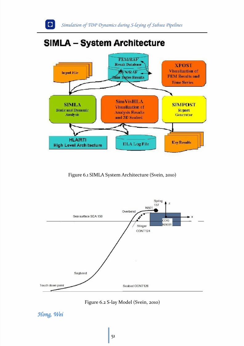
8/11/2019 Cañerías Offshore Instalación
http://slidepdf.com/reader/full/canerias-offshore-instalacion 62/157
Simulation of TDP Dynamics during S-laying of Subsea Pipelines
Hong Wei
51
Figure 6.1 SIMLA System Architecture (Svein, 2010)
Figure 6.2 S-lay Model (Svein, 2010)
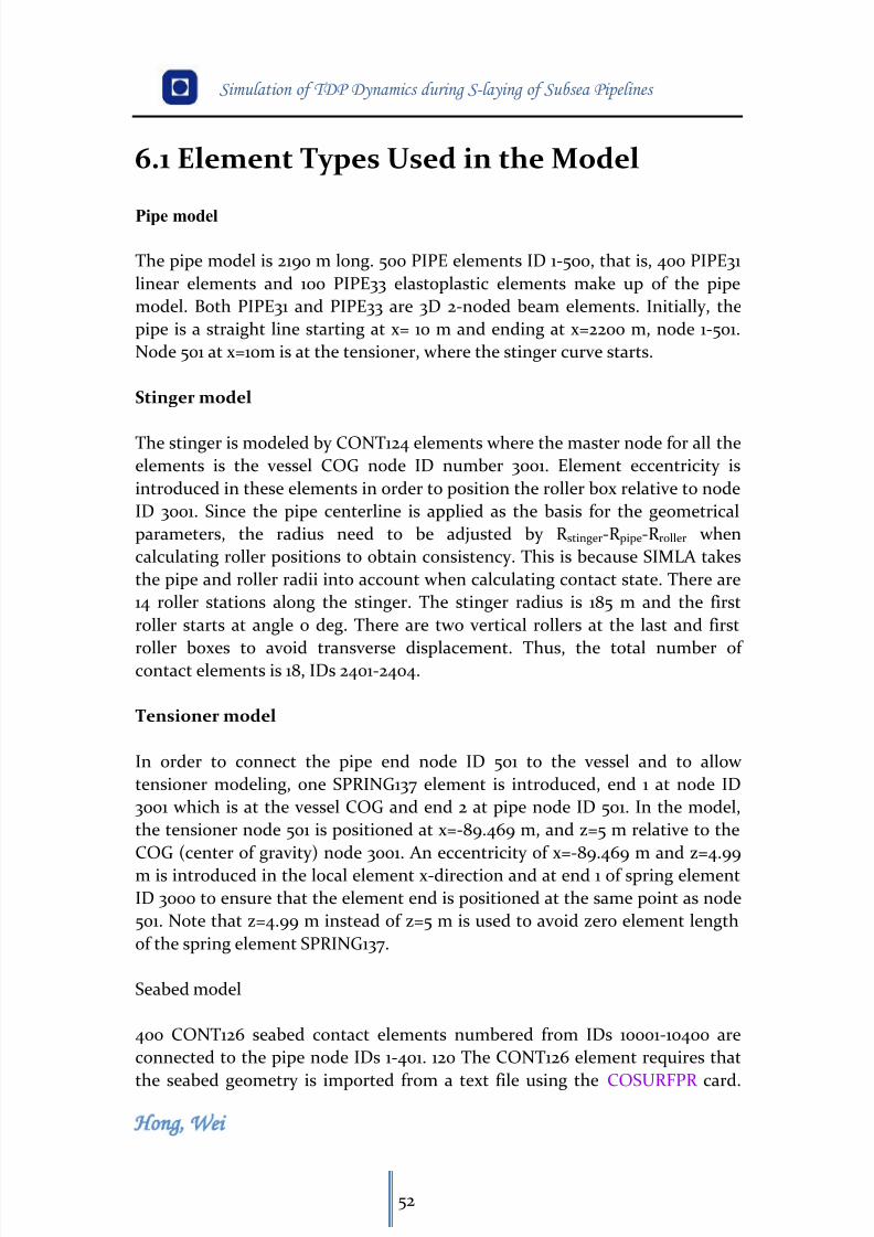
8/11/2019 Cañerías Offshore Instalación
http://slidepdf.com/reader/full/canerias-offshore-instalacion 63/157
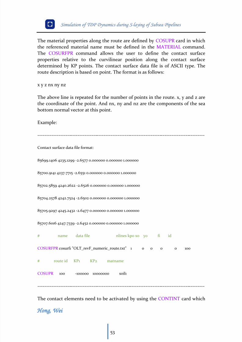
8/11/2019 Cañerías Offshore Instalación
http://slidepdf.com/reader/full/canerias-offshore-instalacion 64/157
Simulation of TDP Dynamics during S-laying of Subsea Pipelines
Hong Wei
53
The material properties along the route are defined by COSUPR card in which
the referenced material name must be defined in the MATERIAL command.
The COSURFPR command allows the user to define the contact surface
properties relative to the curvilinear position along the contact surfacedetermined by KP points. The contact surface data file is of ASCII type. The
route description is based on point. The format is as follows:
x y z nx ny nz
The above line is repeated for the number of points in the route. x, y and z are
the coordinate of the point. And nx, ny and nz are the components of the sea
bottom normal vector at this point.
Example:
------------------------------------------------------------------------------------------------
Contact surface data file format:
85699.1406 4235.1299 -2.6577 0.000000 0.000000 1.000000
85700.9141 4237.7715 -2.6551 0.000000 0.000000 1.000000
85702.5859 4240.2622 -2.6526 0.000000 0.000000 1.000000
85704.2578 4242.7524 -2.6502 0.000000 0.000000 1.000000
85705.9297 4245.2432 -2.6477 0.000000 0.000000 1.000000
85707.6016 4247.7339 -2.6452 0.000000 0.000000 1.000000
# name data file nlines kp0 x0 y0 fi id
COSURFPR cosurf1 "OLT_revF_numeric_route.txt" 1 0 0 0 0 100
# route id KP1 KP2 matname
COSUPR 100 -100000 10000000 soil1
------------------------------------------------------------------------------------------------
The contact elements need to be activated by using the CONTINT card which
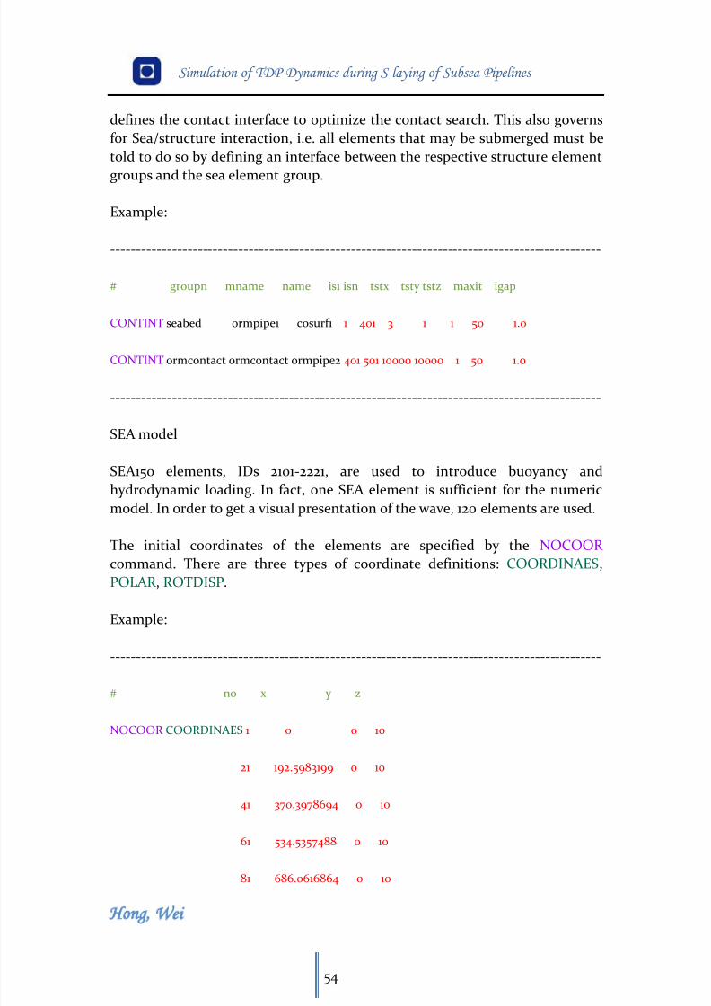
8/11/2019 Cañerías Offshore Instalación
http://slidepdf.com/reader/full/canerias-offshore-instalacion 65/157
Simulation of TDP Dynamics during S-laying of Subsea Pipelines
Hong Wei
54
defines the contact interface to optimize the contact search. This also governs
for Sea/structure interaction, i.e. all elements that may be submerged must be
told to do so by defining an interface between the respective structure element
groups and the sea element group.
Example:
------------------------------------------------------------------------------------------------
# groupn mname name is1 isn tstx tsty tstz maxit igap
CONTINT seabed ormpipe1 cosurf1 1 401 3 1 1 50 1.0
CONTINT ormcontact ormcontact ormpipe2 401 501 10000 10000 1 50 1.0
------------------------------------------------------------------------------------------------
SEA model
SEA150 elements, IDs 2101-2221, are used to introduce buoyancy and
hydrodynamic loading. In fact, one SEA element is sufficient for the numeric
model. In order to get a visual presentation of the wave, 120 elements are used.
The initial coordinates of the elements are specified by the NOCOOR
command. There are three types of coordinate definitions: COORDINAES,
POLAR , ROTDISP.
Example:
------------------------------------------------------------------------------------------------
# no x y z
NOCOOR COORDINAES 1 0 0 10
21 192.5983199 0 10
41 370.3978694 0 10
61 534.5357488 0 10
81 686.0616864 0 10

8/11/2019 Cañerías Offshore Instalación
http://slidepdf.com/reader/full/canerias-offshore-instalacion 66/157
Simulation of TDP Dynamics during S-laying of Subsea Pipelines
Hong Wei
55
101 825.9447521 0 10
------------------------------------------------------------------------------------------------
The initial orientation of the element coordinate systems is defined by
ELORIENT command. For the PIPE and HSHEAR (coating) elements, the
orientations are defined by specifying the position of the xy-plane of the local
element system relative to the global coordinate system. For the SPRING and
CONTACT elements, the orientation of end 1 of the node is defined by
specifying a set of three consecutive Euler angles that rotates the local
coordinate system to the global coordinate system.
Example:
------------------------------------------------------------------------------------------------
# PIPE element
# no x y z
ELORIENT COORDINATES 1 0 10000 10
500 2200 10000 10
#SPRING element
ELORIENT EULERANGLE 3000 0 0 0
------------------------------------------------------------------------------------------------
The element properties are defined by the ELPROP command. In SIMLA, there
are 9 types of element properties available: PIPE, BELLMOUTH, COMPIPE,
CABLE, ROLLER , USERCONTACT, GENSPRING, COATING, BODY . In this
model, PIPE, ROLLER and GENSPRING are used.
------------------------------------------------------------------------------------------------
# name type rad th CDr Cdt CMr CMt wd ws
ELPROP ormpipe1 pipe 0.525 0.0341 0.8 0.1 2.0 0.2 1.291 0.161
ODp ODw rks
8/11/2019 Cañerías Offshore Instalación
http://slidepdf.com/reader/full/canerias-offshore-instalacion 67/157
8/11/2019 Cañerías Offshore Instalación
http://slidepdf.com/reader/full/canerias-offshore-instalacion 68/157
Simulation of TDP Dynamics during S-laying of Subsea Pipelines
Hong Wei
57
them, LINEAR , ELASTOPLASTIC, EPCURVE, HYCURVE, SEA , CONTACT,
GENSPRING are applied in this model.
LINEAR represents linear material properties for the elastic pipe element. Inthe option, the poisson’s ratio, axial stiffness, bending stiffness, torsion stiffness,
young’s modulus, shear modulus and so on are specified.
------------------------------------------------------------------------------------------------
# name type poiss talfa tecond heatc beta ea
MATERIAL pipemat1 linear 0.3 1.17e-5 50 800 0 2.249e7
eiy eiz git em gm
3.10e6 3.10e6 2.39e6 2e8 8e7
------------------------------------------------------------------------------------------------
ELASTOPLASTIC represents elastic strain-stress behavior with
kinematic/isotropic hardening for the elastoplastic pipe elements. Any number
of pairs of strain and stress can be given and linear interpolation is applied
between the supplied data. Either kinematic hardening or isotropic hardeningis applied.
------------------------------------------------------------------------------------------------
# name type ih poiss ro talfa tec hc eps sigma
MATERIAL pipemat2 elastoplastic 1 0.3 7.850 1.17e-5 50 800 0 0
1.691E-03 3.50E+05
0.005 4.50E+05
9.980E-02 8.35E+05
------------------------------------------------------------------------------------------------
EPCURVE represents elastoplastic material behavior with kinematic/isotropic
hardening. And HYCURVE represents hyperelastic (nonlinear elastic) material
behavior.
8/11/2019 Cañerías Offshore Instalación
http://slidepdf.com/reader/full/canerias-offshore-instalacion 69/157
Simulation of TDP Dynamics during S-laying of Subsea Pipelines
Hong Wei
58
In the model, the seabed is considered made up of 3D elastoplastic spring
elements. In the x,y direction, EPCURVE model is used and HYCURVE model is
applied in z direction.
------------------------------------------------------------------------------------------------
# seabed soil
# name type rmyx rmyy xname yname zname
MATERIAL soil1 contact 0.5 1.0 soilx soily soilz
MATERIAL soil2 contact 0.5 1.0 soilx soily soilz2
# name type alfa eps sig
MATERIAL soilx epcurve 1 0 0
0.005 1
100.00 10
# name type eps sig
MATERIAL soilz hycurve -10000 -10000000
10000 10000000
# Tensioner
# name type apr1 spr2 spr3 spr4 spr5 spr6
MATERIAL vessel1 genspring surgesp1 yawsp heavesp rollsp pitchsp swaysp
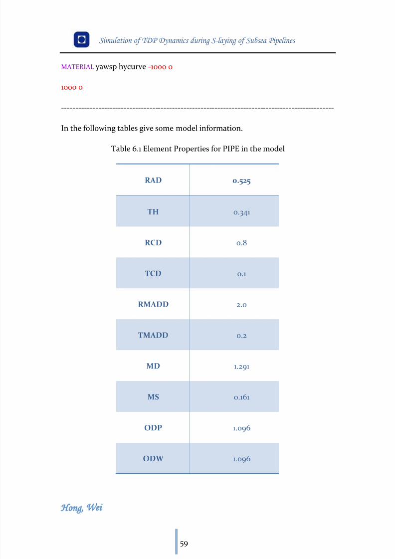
8/11/2019 Cañerías Offshore Instalación
http://slidepdf.com/reader/full/canerias-offshore-instalacion 70/157
Simulation of TDP Dynamics during S-laying of Subsea Pipelines
Hong Wei
59
MATERIAL yawsp hycurve -1000 0
1000 0
------------------------------------------------------------------------------------------------
In the following tables give some model information.
Table 6.1 Element Properties for PIPE in the model
RAD 0.525
TH 0.341
RCD 0.8
TCD 0.1
RMADD 2.0
TMADD 0.2
MD 1.291
MS 0.161
ODP 1.096
ODW 1.096
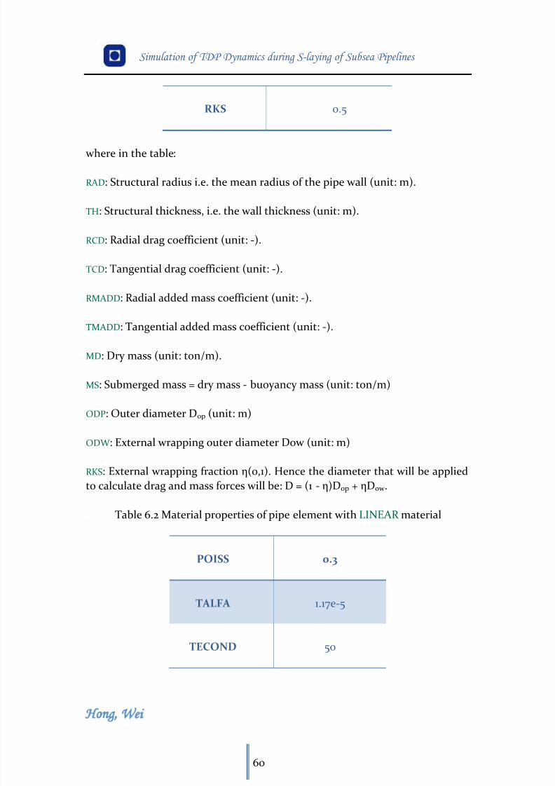
8/11/2019 Cañerías Offshore Instalación
http://slidepdf.com/reader/full/canerias-offshore-instalacion 71/157
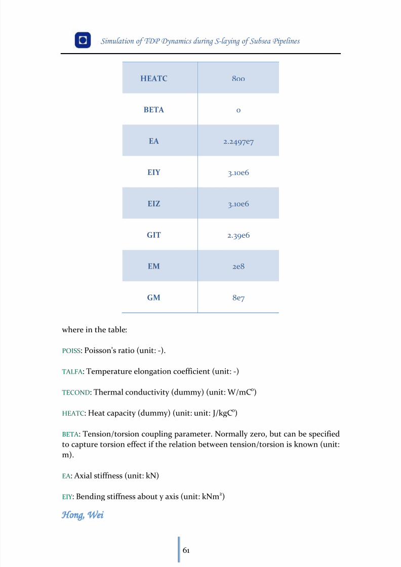
8/11/2019 Cañerías Offshore Instalación
http://slidepdf.com/reader/full/canerias-offshore-instalacion 72/157
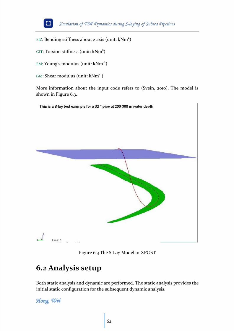
8/11/2019 Cañerías Offshore Instalación
http://slidepdf.com/reader/full/canerias-offshore-instalacion 73/157
Simulation of TDP Dynamics during S-laying of Subsea Pipelines
Hong Wei
62
EIZ: Bending stiffness about z axis (unit: kNm2)
GIT: Torsion stiffness (unit: kNm2)
EM: Young's modulus (unit: kNm-2)
GM: Shear modulus (unit: kNm-2)
More information about the input code refers to (Svein, 2010). The model is
shown in Figure 6.3.
Figure 6.3 The S-Lay Model in XPOST
6.2 Analysis setup
Both static analysis and dynamic are performed. The static analysis provides the
initial static configuration for the subsequent dynamic analysis.
8/11/2019 Cañerías Offshore Instalación
http://slidepdf.com/reader/full/canerias-offshore-instalacion 74/157
Simulation of TDP Dynamics during S-laying of Subsea Pipelines
Hong Wei
63
The static analysis is done in one load step using the AUTOSTART feature that
enables initiation of S-lay. The static and dynamic analysis is defined in two
sequences using the TIMECO card, steps 0-1 with step length 1 s for static
analysis and then steps 1.1 s-3600 s with 0.1 s step length for dynamic analysis.In order to get enough results to observe the dynamic behaviors of the
touchdown point (TDP), the simulation time is set to 3600 s. For each case, the
total running time is more or less 6 hours. In our case, two TIMECO cards are
used for dynamic analysis to avoid too large .raf file. The first card for dynamic
analysis sets the time increment between each restart and visual storage to
the .raf file is 1 sec. And for the second one, it is set to be 10 sec.
------------------------------------------------------------------------------------------------
# t dt dtvi dtdy dt0 type hla? Steptype iter itcrit
TIMECO 1.0 1.0 1.0 1.0 201.0 STATIC NOHLA
TIMECO 360.0 0.10 1.0 1.0 201.0 DYNAMIC NOHLA auto none all 20 5 1.0e-4
TIMECO 3600.0 0.10 10.0 1.0 201.0 DYNAMIC NOHLA auto none all 20 5 1.0e-4
------------------------------------------------------------------------------------------------
For the static analysis gravity loading is applied in one step to the full value.
Note that in this case, the material properties for the SPRING137 vessel element
have set to zero as the displacement of node 501 is kinematically fully described
by using the CONSTR PDISP SPECIAL option for node 501 using the
eccentricities between node ID 3001 and node ID 501and the CONSTR PDISP
RAO for node 3001 which is the vessel. For the dynamic analysis, the full value
of tension is applied in element ID 500 as a concentrated load in node 501 by
the CLOAD command. The concentrated nodal loads are defined in the global
coordinate system.
------------------------------------------------------------------------------------------------# sn dof mn fi1 fi2 fi3 ex ey ez
CONSTR PDISP SPECIAL 501 1 3001 0 0.0 0 -89.469 0 5.000
CONSTR PDISP SPECIAL 501 2 3001 0 0.0 0 -89.469 0 5.000
CONSTR PDISP SPECIAL 501 3 3001 0 0.0 0 -89.469 0 5.000
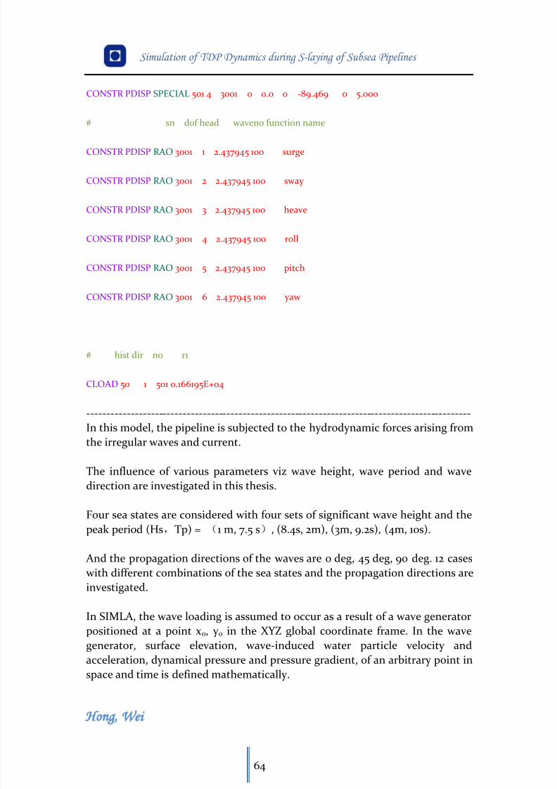
8/11/2019 Cañerías Offshore Instalación
http://slidepdf.com/reader/full/canerias-offshore-instalacion 75/157
Simulation of TDP Dynamics during S-laying of Subsea Pipelines
Hong Wei
64
CONSTR PDISP SPECIAL 501 4 3001 0 0.0 0 -89.469 0 5.000
# sn d0f head waveno function name
CONSTR PDISP RAO 3001 1 2.437945 100 surge
CONSTR PDISP RAO 3001 2 2.437945 100 sway
CONSTR PDISP RAO 3001 3 2.437945 100 heave
CONSTR PDISP RAO 3001 4 2.437945 100 roll
CONSTR PDISP RAO 3001 5 2.437945 100 pitch
CONSTR PDISP RAO 3001 6 2.437945 100 yaw
# hist dir no r1
CLOAD 50 1 501 0.166195E+04
------------------------------------------------------------------------------------------------In this model, the pipeline is subjected to the hydrodynamic forces arising from
the irregular waves and current.
The influence of various parameters viz wave height, wave period and wave
direction are investigated in this thesis.
Four sea states are considered with four sets of significant wave height and the
peak period (Hs,Tp) = (1 m, 7.5 s), (8.4s, 2m), (3m, 9.2s), (4m, 10s).
And the propagation directions of the waves are 0 deg, 45 deg, 90 deg. 12 cases
with different combinations of the sea states and the propagation directions are
investigated.
In SIMLA, the wave loading is assumed to occur as a result of a wave generator
positioned at a point x0, y 0 in the XYZ global coordinate frame. In the wave
generator, surface elevation, wave-induced water particle velocity and
acceleration, dynamical pressure and pressure gradient, of an arbitrary point in
space and time is defined mathematically.
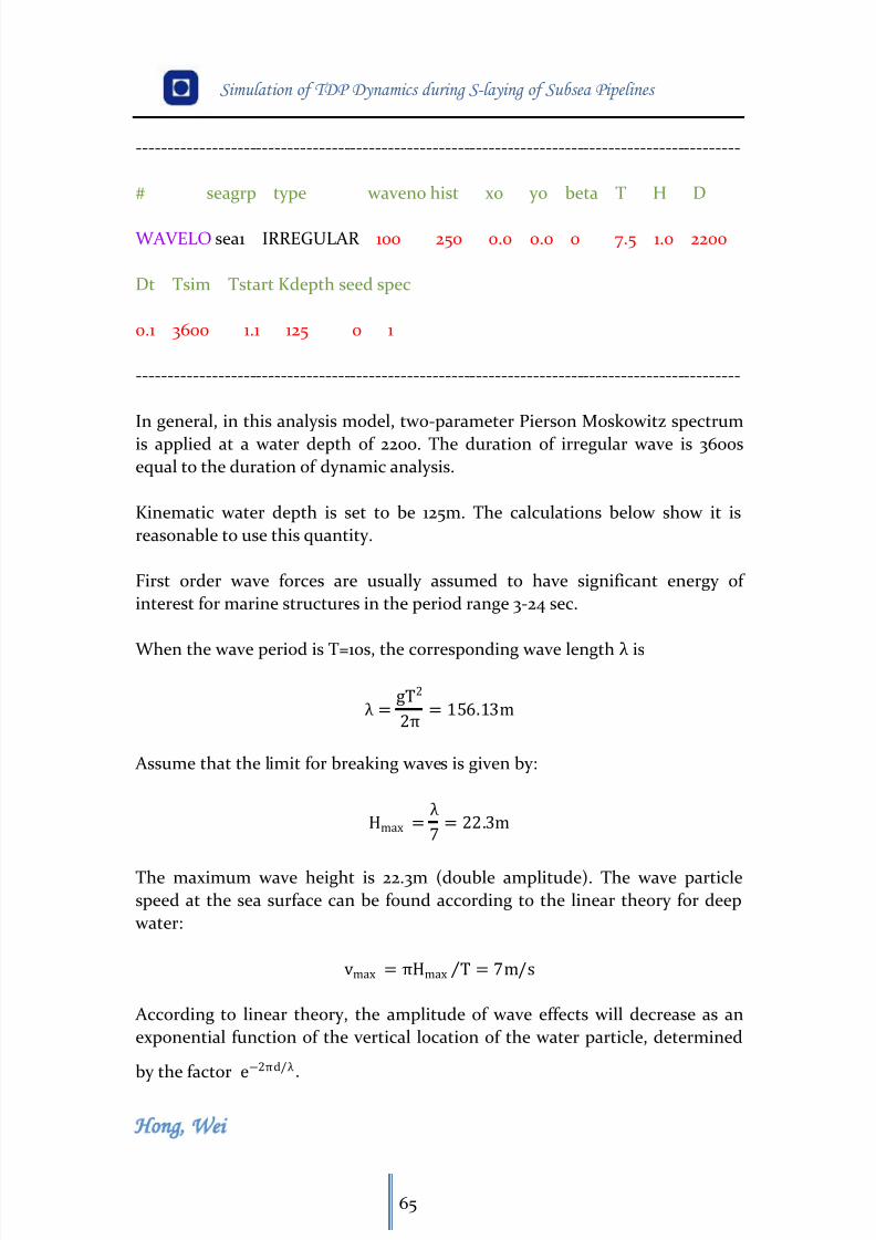
8/11/2019 Cañerías Offshore Instalación
http://slidepdf.com/reader/full/canerias-offshore-instalacion 76/157
Simulation of TDP Dynamics during S-laying of Subsea Pipelines
Hong Wei
65
------------------------------------------------------------------------------------------------
# seagrp type waveno hist x0 y0 beta T H D
WAVELO sea1 IRREGULAR 100 250 0.0 0.0 0 7.5 1.0 2200
Dt Tsim Tstart Kdepth seed spec
0.1 3600 1.1 125 0 1
------------------------------------------------------------------------------------------------
In general, in this analysis model, two-parameter Pierson Moskowitz spectrum
is applied at a water depth of 2200. The duration of irregular wave is 3600s
equal to the duration of dynamic analysis.
Kinematic water depth is set to be 125m. The calculations below show it is
reasonable to use this quantity.
First order wave forces are usually assumed to have significant energy of
interest for marine structures in the period range 3-24 sec.
When the wave period is T=10s, the corresponding wave length λ is
λ =gT2
2π = 156.13m
Assume that the limit for breaking waves is given by:
Hmax =λ7
= 22.3m
The maximum wave height is 22.3m (double amplitude). The wave particle
speed at the sea surface can be found according to the linear theory for deep
water:
vmax = πHmax T = 7m/s
According to linear theory, the amplitude of wave effects will decrease as an
exponential function of the vertical location of the water particle, determined
by the factor e
−2
πd/
λ.
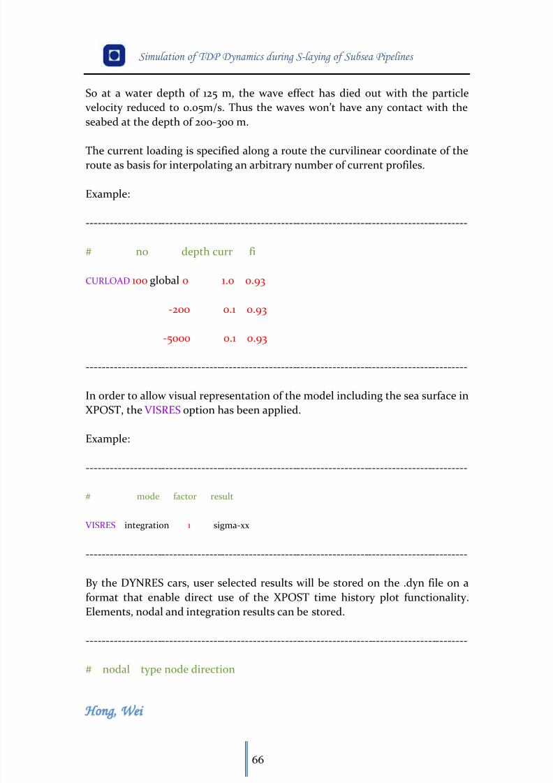
8/11/2019 Cañerías Offshore Instalación
http://slidepdf.com/reader/full/canerias-offshore-instalacion 77/157
Simulation of TDP Dynamics during S-laying of Subsea Pipelines
Hong Wei
66
So at a water depth of 125 m, the wave effect has died out with the particle
velocity reduced to 0.05m/s. Thus the waves won’t have any contact with the
seabed at the depth of 200-300 m.
The current loading is specified along a route the curvilinear coordinate of the
route as basis for interpolating an arbitrary number of current profiles.
Example:
------------------------------------------------------------------------------------------------
# no depth curr fi
CURLOAD 100 global 0 1.0 0.93
-200 0.1 0.93
-5000 0.1 0.93
------------------------------------------------------------------------------------------------
In order to allow visual representation of the model including the sea surface in
XPOST, the VISRES option has been applied.
Example:
------------------------------------------------------------------------------------------------
# mode factor result
VISRES integration 1 sigma-xx
------------------------------------------------------------------------------------------------
By the DYNRES cars, user selected results will be stored on the .dyn file on a
format that enable direct use of the XPOST time history plot functionality.
Elements, nodal and integration results can be stored.
------------------------------------------------------------------------------------------------
# nodal type node direction
8/11/2019 Cañerías Offshore Instalación
http://slidepdf.com/reader/full/canerias-offshore-instalacion 78/157
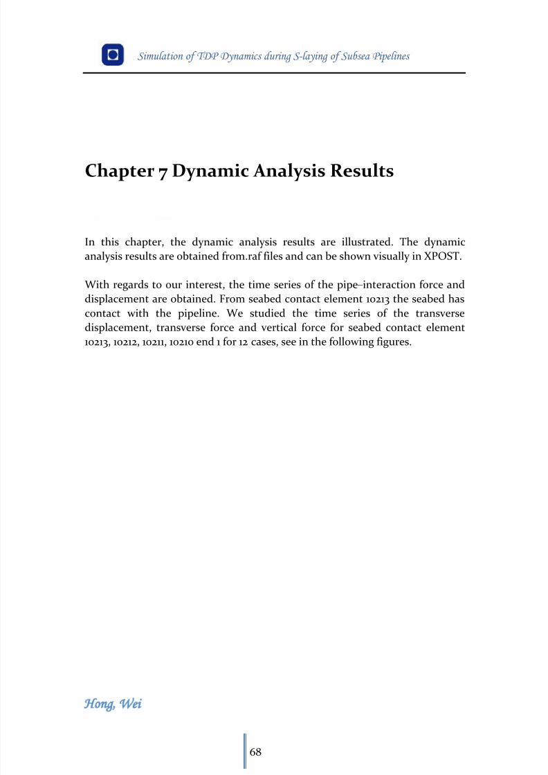
8/11/2019 Cañerías Offshore Instalación
http://slidepdf.com/reader/full/canerias-offshore-instalacion 79/157
Simulation of TDP Dynamics during S-laying of Subsea Pipelines
Hong Wei
68
Chapter 7 Dynamic Analysis Results
In this chapter, the dynamic analysis results are illustrated. The dynamic
analysis results are obtained from.raf files and can be shown visually in XPOST.
With regards to our interest, the time series of the pipe–interaction force and
displacement are obtained. From seabed contact element 10213 the seabed has
contact with the pipeline. We studied the time series of the transverse
displacement, transverse force and vertical force for seabed contact element
10213, 10212, 10211, 10210 end 1 for 12 cases, see in the following figures.
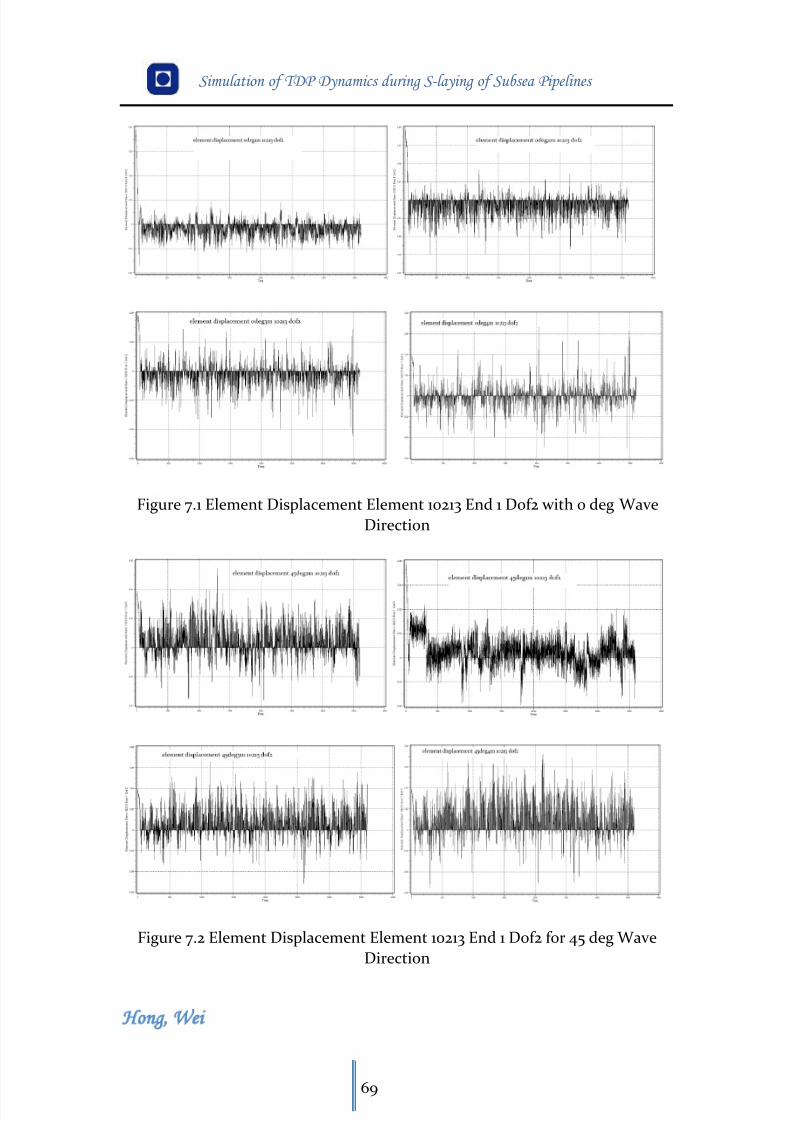
8/11/2019 Cañerías Offshore Instalación
http://slidepdf.com/reader/full/canerias-offshore-instalacion 80/157
Simulation of TDP Dynamics during S-laying of Subsea Pipelines
Hong Wei
69
Figure 7.1 Element Displacement Element 10213 End 1 Dof2 with 0 deg Wave
Direction
Figure 7.2 Element Displacement Element 10213 End 1 Dof2 for 45 deg Wave
Direction
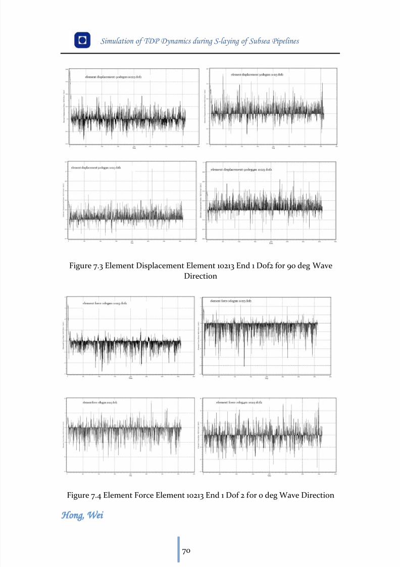
8/11/2019 Cañerías Offshore Instalación
http://slidepdf.com/reader/full/canerias-offshore-instalacion 81/157
Simulation of TDP Dynamics during S-laying of Subsea Pipelines
Hong Wei
70
Figure 7.3 Element Displacement Element 10213 End 1 Dof2 for 90 deg Wave
Direction
Figure 7.4 Element Force Element 10213 End 1 Dof 2 for 0 deg Wave Direction
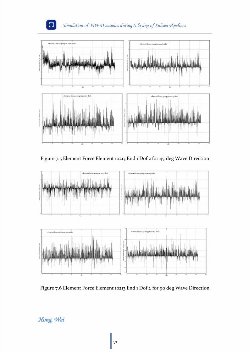
8/11/2019 Cañerías Offshore Instalación
http://slidepdf.com/reader/full/canerias-offshore-instalacion 82/157
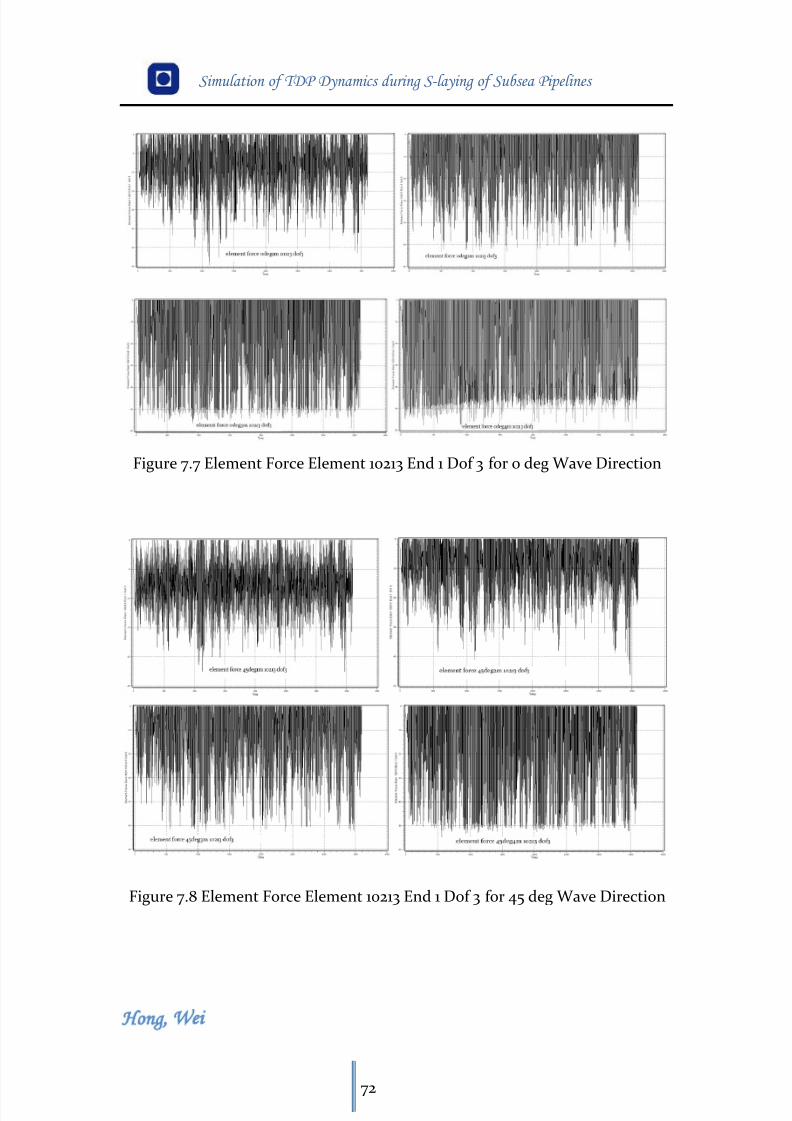
8/11/2019 Cañerías Offshore Instalación
http://slidepdf.com/reader/full/canerias-offshore-instalacion 83/157
Simulation of TDP Dynamics during S-laying of Subsea Pipelines
Hong Wei
72
Figure 7.7 Element Force Element 10213 End 1 Dof 3 for 0 deg Wave Direction
Figure 7.8 Element Force Element 10213 End 1 Dof 3 for 45 deg Wave Direction
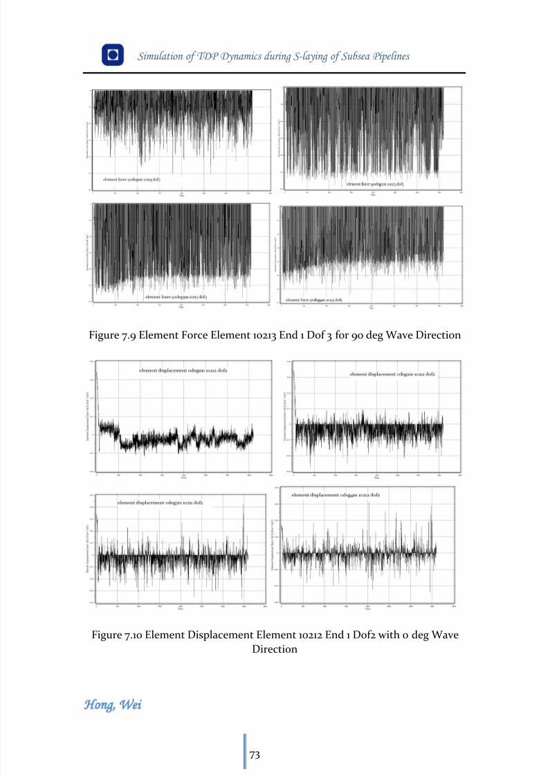
8/11/2019 Cañerías Offshore Instalación
http://slidepdf.com/reader/full/canerias-offshore-instalacion 84/157
Simulation of TDP Dynamics during S-laying of Subsea Pipelines
Hong Wei
73
Figure 7.9 Element Force Element 10213 End 1 Dof 3 for 90 deg Wave Direction
Figure 7.10 Element Displacement Element 10212 End 1 Dof2 with 0 deg Wave
Direction
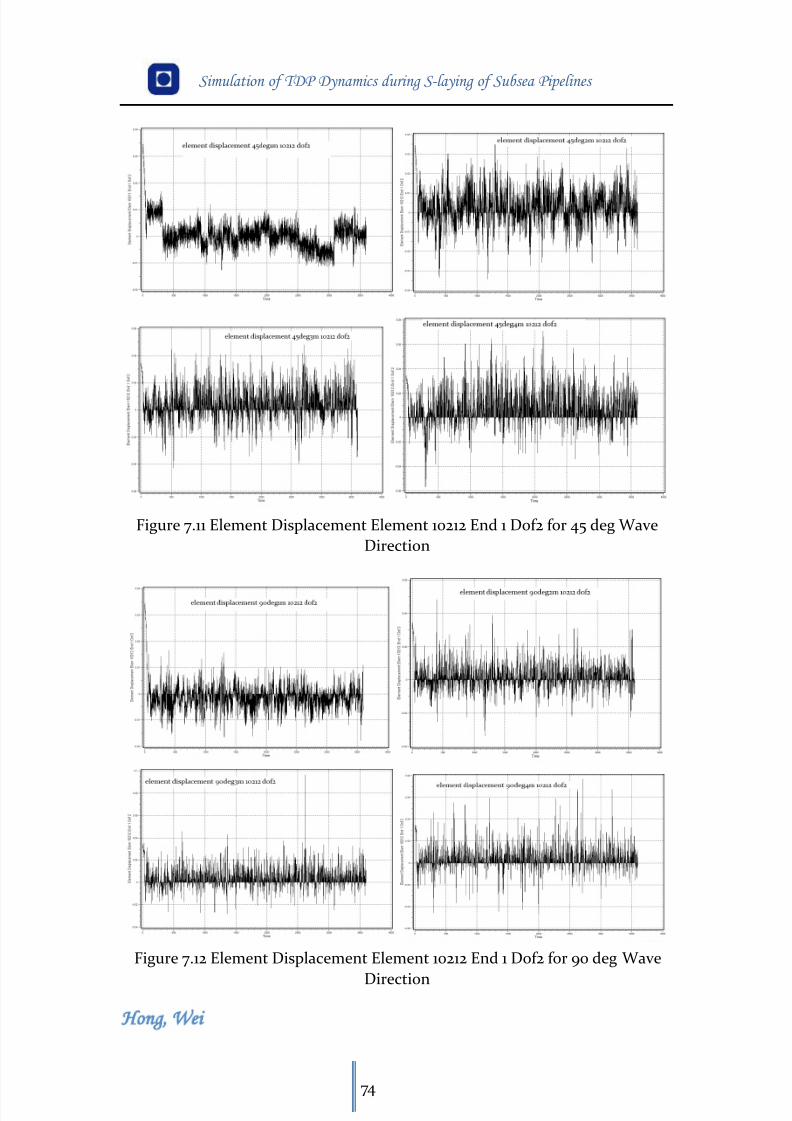
8/11/2019 Cañerías Offshore Instalación
http://slidepdf.com/reader/full/canerias-offshore-instalacion 85/157
Simulation of TDP Dynamics during S-laying of Subsea Pipelines
Hong Wei
74
Figure 7.11 Element Displacement Element 10212 End 1 Dof2 for 45 deg Wave
Direction
Figure 7.12 Element Displacement Element 10212 End 1 Dof2 for 90 deg Wave
Direction
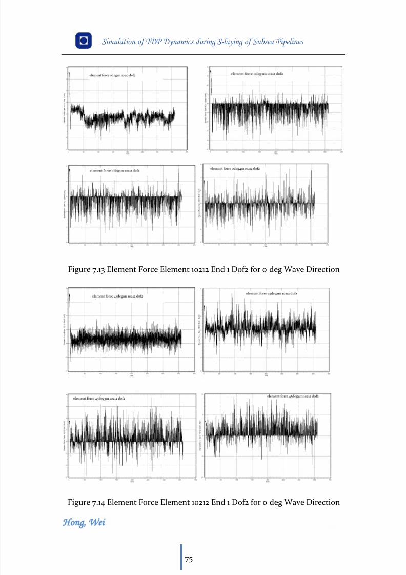
8/11/2019 Cañerías Offshore Instalación
http://slidepdf.com/reader/full/canerias-offshore-instalacion 86/157
Simulation of TDP Dynamics during S-laying of Subsea Pipelines
Hong Wei
75
Figure 7.13 Element Force Element 10212 End 1 Dof2 for 0 deg Wave Direction
Figure 7.14 Element Force Element 10212 End 1 Dof2 for 0 deg Wave Direction
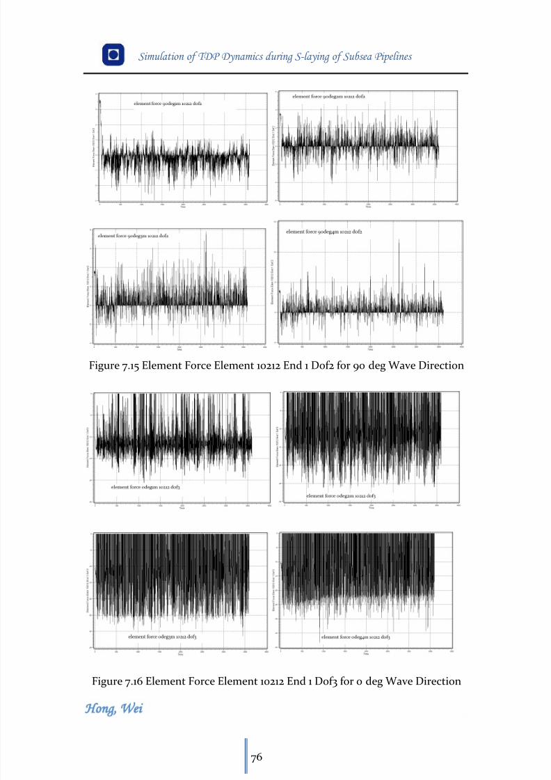
8/11/2019 Cañerías Offshore Instalación
http://slidepdf.com/reader/full/canerias-offshore-instalacion 87/157
Simulation of TDP Dynamics during S-laying of Subsea Pipelines
Hong Wei
76
Figure 7.15 Element Force Element 10212 End 1 Dof2 for 90 deg Wave Direction
Figure 7.16 Element Force Element 10212 End 1 Dof3 for 0 deg Wave Direction
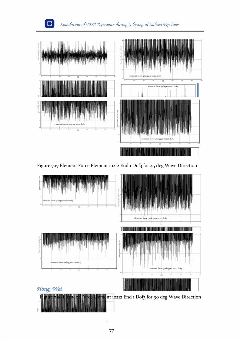
8/11/2019 Cañerías Offshore Instalación
http://slidepdf.com/reader/full/canerias-offshore-instalacion 88/157
Simulation of TDP Dynamics during S-laying of Subsea Pipelines
Hong Wei
77
Figure 7.17 Element Force Element 10212 End 1 Dof3 for 45 deg Wave Direction
Figure 7.18 Element Force Element 10212 End 1 Dof3 for 90 deg Wave Direction
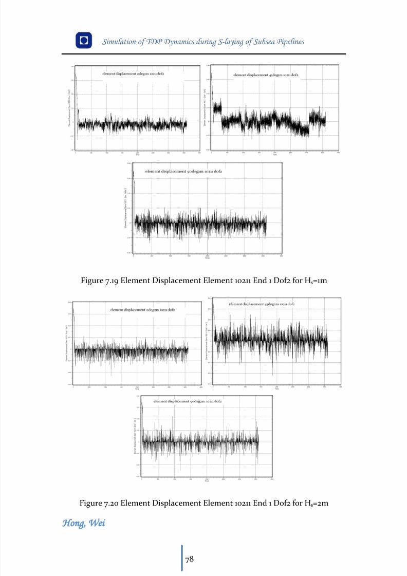
8/11/2019 Cañerías Offshore Instalación
http://slidepdf.com/reader/full/canerias-offshore-instalacion 89/157
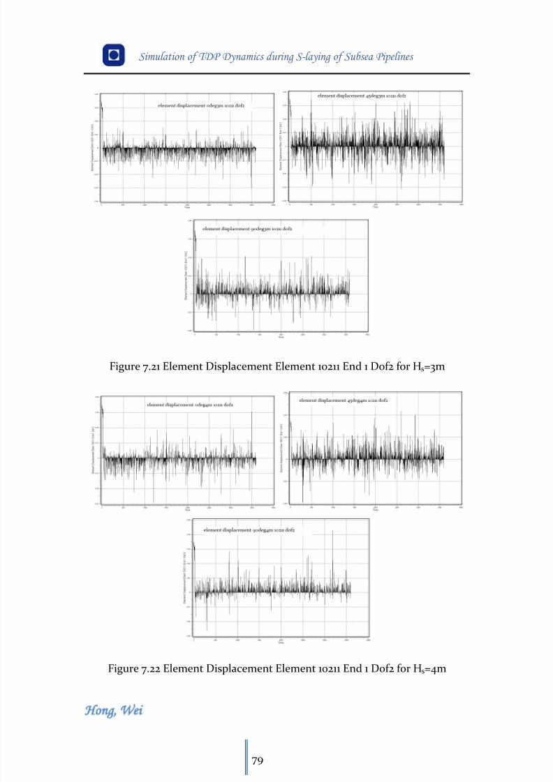
8/11/2019 Cañerías Offshore Instalación
http://slidepdf.com/reader/full/canerias-offshore-instalacion 90/157
Simulation of TDP Dynamics during S-laying of Subsea Pipelines
Hong Wei
79
Figure 7.21 Element Displacement Element 10211 End 1 Dof2 for Hs=3m
Figure 7.22 Element Displacement Element 10211 End 1 Dof2 for Hs=4m
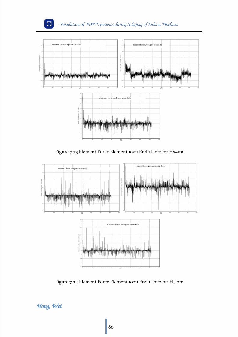
8/11/2019 Cañerías Offshore Instalación
http://slidepdf.com/reader/full/canerias-offshore-instalacion 91/157
Simulation of TDP Dynamics during S-laying of Subsea Pipelines
Hong Wei
80
Figure 7.23 Element Force Element 10211 End 1 Dof2 for Hs=1m
Figure 7.24 Element Force Element 10211 End 1 Dof2 for Hs=2m
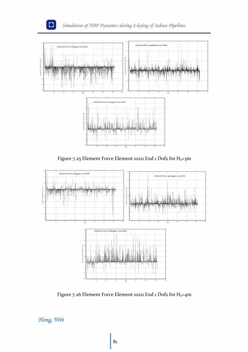
8/11/2019 Cañerías Offshore Instalación
http://slidepdf.com/reader/full/canerias-offshore-instalacion 92/157
Simulation of TDP Dynamics during S-laying of Subsea Pipelines
Hong Wei
81
Figure 7.25 Element Force Element 10211 End 1 Dof2 for Hs=3m
Figure 7.26 Element Force Element 10211 End 1 Dof2 for Hs=4m
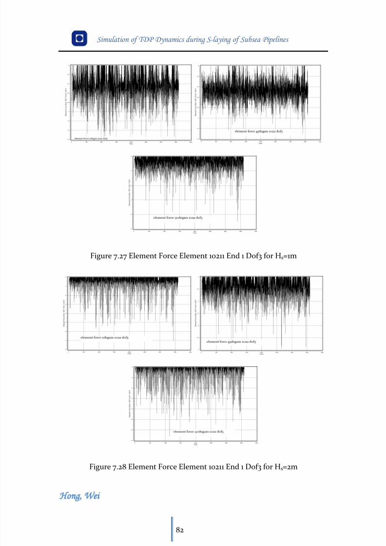
8/11/2019 Cañerías Offshore Instalación
http://slidepdf.com/reader/full/canerias-offshore-instalacion 93/157
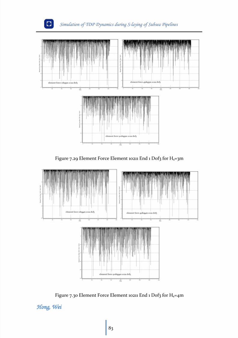
8/11/2019 Cañerías Offshore Instalación
http://slidepdf.com/reader/full/canerias-offshore-instalacion 94/157
Simulation of TDP Dynamics during S-laying of Subsea Pipelines
Hong Wei
83
Figure 7.29 Element Force Element 10211 End 1 Dof3 for Hs=3m
Figure 7.30 Element Force Element 10211 End 1 Dof3 for Hs=4m
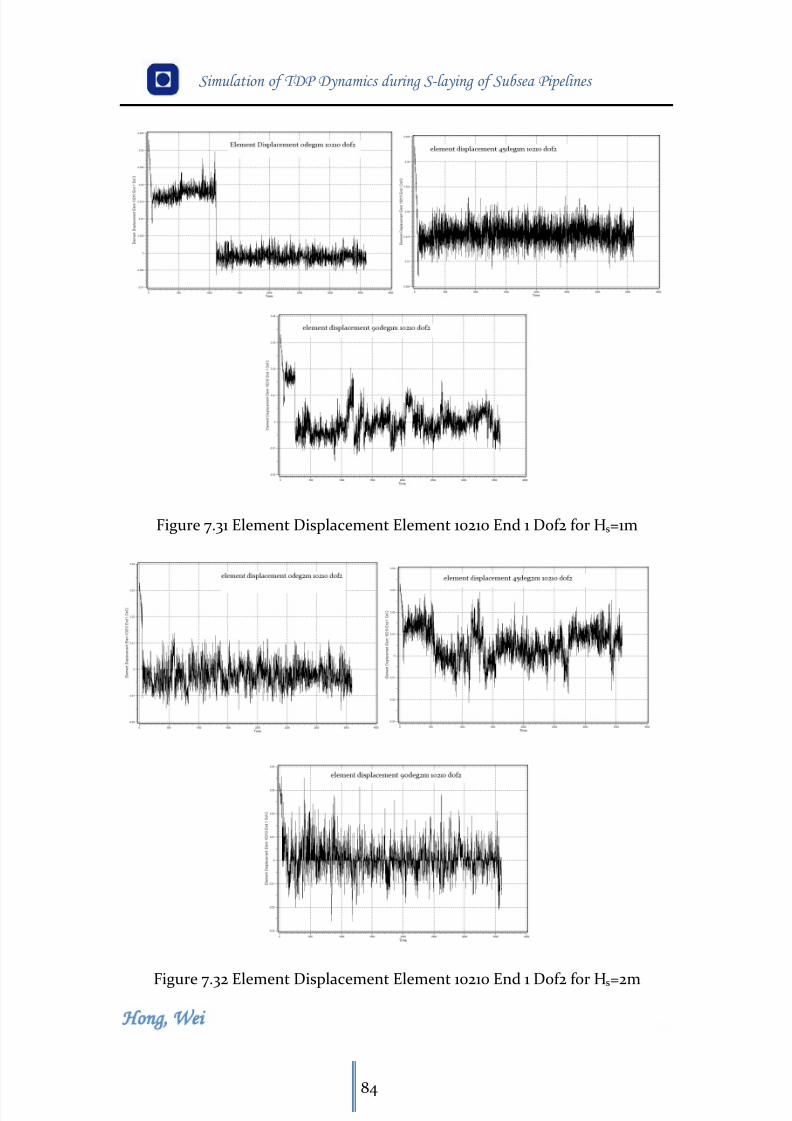
8/11/2019 Cañerías Offshore Instalación
http://slidepdf.com/reader/full/canerias-offshore-instalacion 95/157
Simulation of TDP Dynamics during S-laying of Subsea Pipelines
Hong Wei
84
Figure 7.31 Element Displacement Element 10210 End 1 Dof2 for Hs=1m
Figure 7.32 Element Displacement Element 10210 End 1 Dof2 for Hs=2m
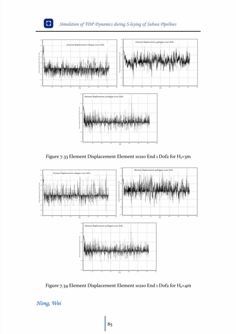
8/11/2019 Cañerías Offshore Instalación
http://slidepdf.com/reader/full/canerias-offshore-instalacion 96/157
Simulation of TDP Dynamics during S-laying of Subsea Pipelines
Hong Wei
85
Figure 7.33 Element Displacement Element 10210 End 1 Dof2 for Hs=3m
Figure 7.34 Element Displacement Element 10210 End 1 Dof2 for Hs=4m
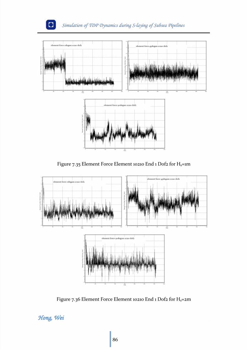
8/11/2019 Cañerías Offshore Instalación
http://slidepdf.com/reader/full/canerias-offshore-instalacion 97/157
Simulation of TDP Dynamics during S-laying of Subsea Pipelines
Hong Wei
86
Figure 7.35 Element Force Element 10210 End 1 Dof2 for Hs=1m
Figure 7.36 Element Force Element 10210 End 1 Dof2 for Hs=2m
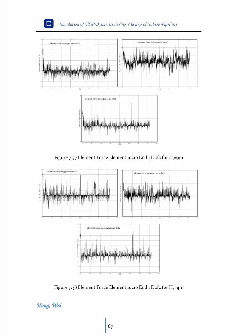
8/11/2019 Cañerías Offshore Instalación
http://slidepdf.com/reader/full/canerias-offshore-instalacion 98/157
Simulation of TDP Dynamics during S-laying of Subsea Pipelines
Hong Wei
87
Figure 7.37 Element Force Element 10210 End 1 Dof2 for Hs=3m
Figure 7.38 Element Force Element 10210 End 1 Dof2 for Hs=4m
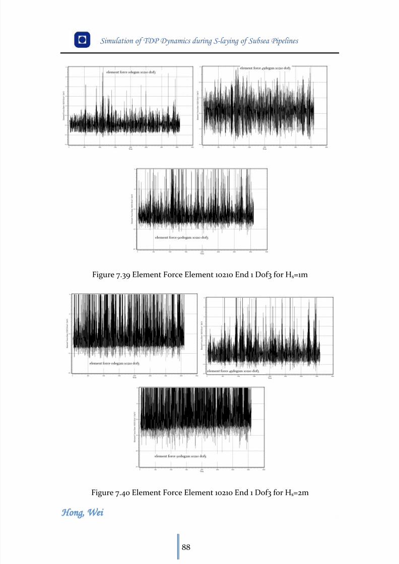
8/11/2019 Cañerías Offshore Instalación
http://slidepdf.com/reader/full/canerias-offshore-instalacion 99/157
Simulation of TDP Dynamics during S-laying of Subsea Pipelines
Hong Wei
88
Figure 7.39 Element Force Element 10210 End 1 Dof3 for Hs=1m
Figure 7.40 Element Force Element 10210 End 1 Dof3 for Hs=2m
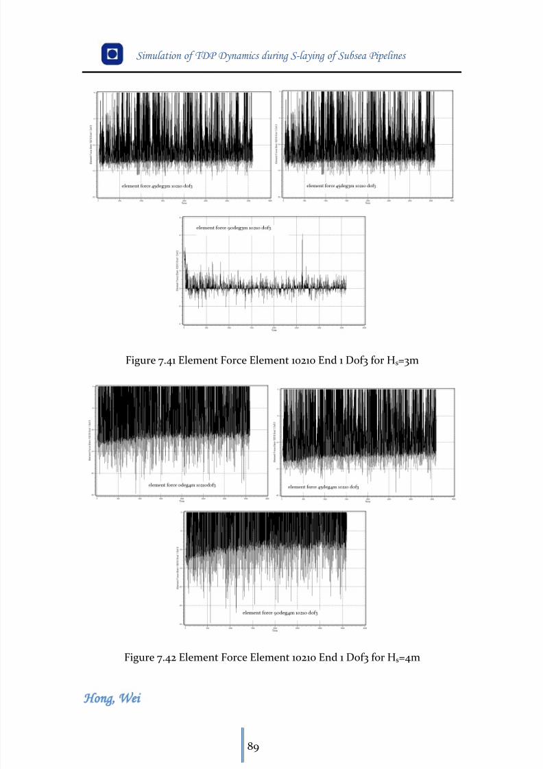
8/11/2019 Cañerías Offshore Instalación
http://slidepdf.com/reader/full/canerias-offshore-instalacion 100/157
Simulation of TDP Dynamics during S-laying of Subsea Pipelines
Hong Wei
89
Figure 7.41 Element Force Element 10210 End 1 Dof3 for Hs=3m
Figure 7.42 Element Force Element 10210 End 1 Dof3 for Hs=4m
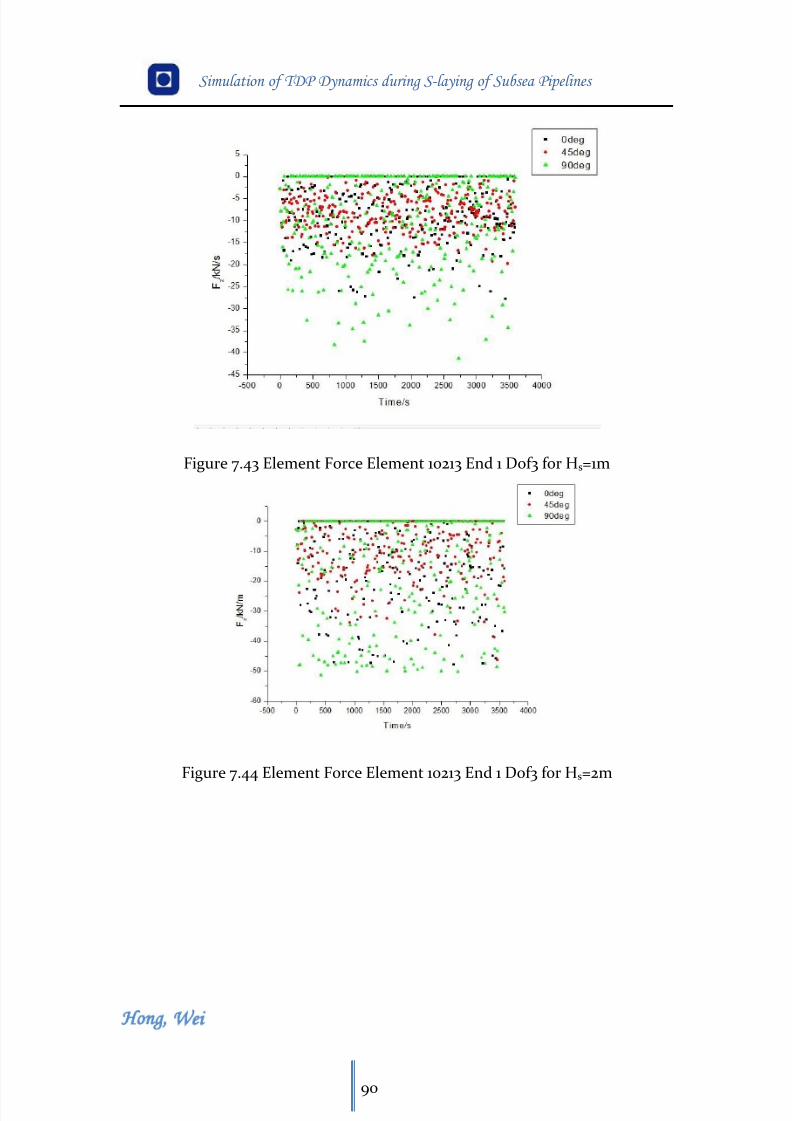
8/11/2019 Cañerías Offshore Instalación
http://slidepdf.com/reader/full/canerias-offshore-instalacion 101/157
Simulation of TDP Dynamics during S-laying of Subsea Pipelines
Hong Wei
90
Figure 7.43 Element Force Element 10213 End 1 Dof3 for Hs=1m
Figure 7.44 Element Force Element 10213 End 1 Dof3 for Hs=2m
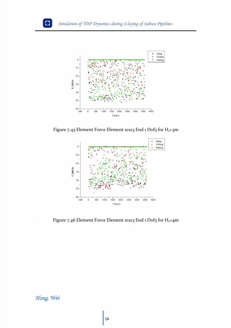
8/11/2019 Cañerías Offshore Instalación
http://slidepdf.com/reader/full/canerias-offshore-instalacion 102/157
Simulation of TDP Dynamics during S-laying of Subsea Pipelines
Hong Wei
91
Figure 7.45 Element Force Element 10213 End 1 Dof3 for Hs=3m
Figure 7.46 Element Force Element 10213 End 1 Dof3 for Hs=4m
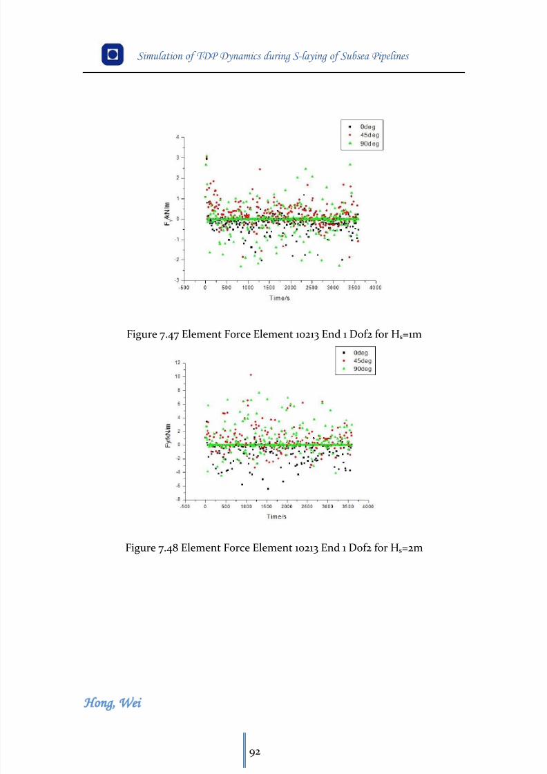
8/11/2019 Cañerías Offshore Instalación
http://slidepdf.com/reader/full/canerias-offshore-instalacion 103/157
Simulation of TDP Dynamics during S-laying of Subsea Pipelines
Hong Wei
92
Figure 7.47 Element Force Element 10213 End 1 Dof2 for Hs=1m
Figure 7.48 Element Force Element 10213 End 1 Dof2 for Hs=2m
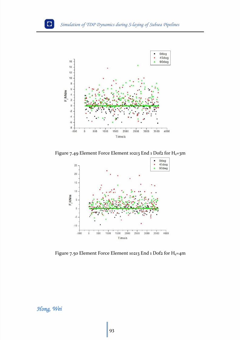
8/11/2019 Cañerías Offshore Instalación
http://slidepdf.com/reader/full/canerias-offshore-instalacion 104/157
Simulation of TDP Dynamics during S-laying of Subsea Pipelines
Hong Wei
93
Figure 7.49 Element Force Element 10213 End 1 Dof2 for Hs=3m
Figure 7.50 Element Force Element 10213 End 1 Dof2 for Hs=4m
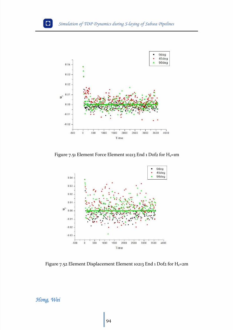
8/11/2019 Cañerías Offshore Instalación
http://slidepdf.com/reader/full/canerias-offshore-instalacion 105/157
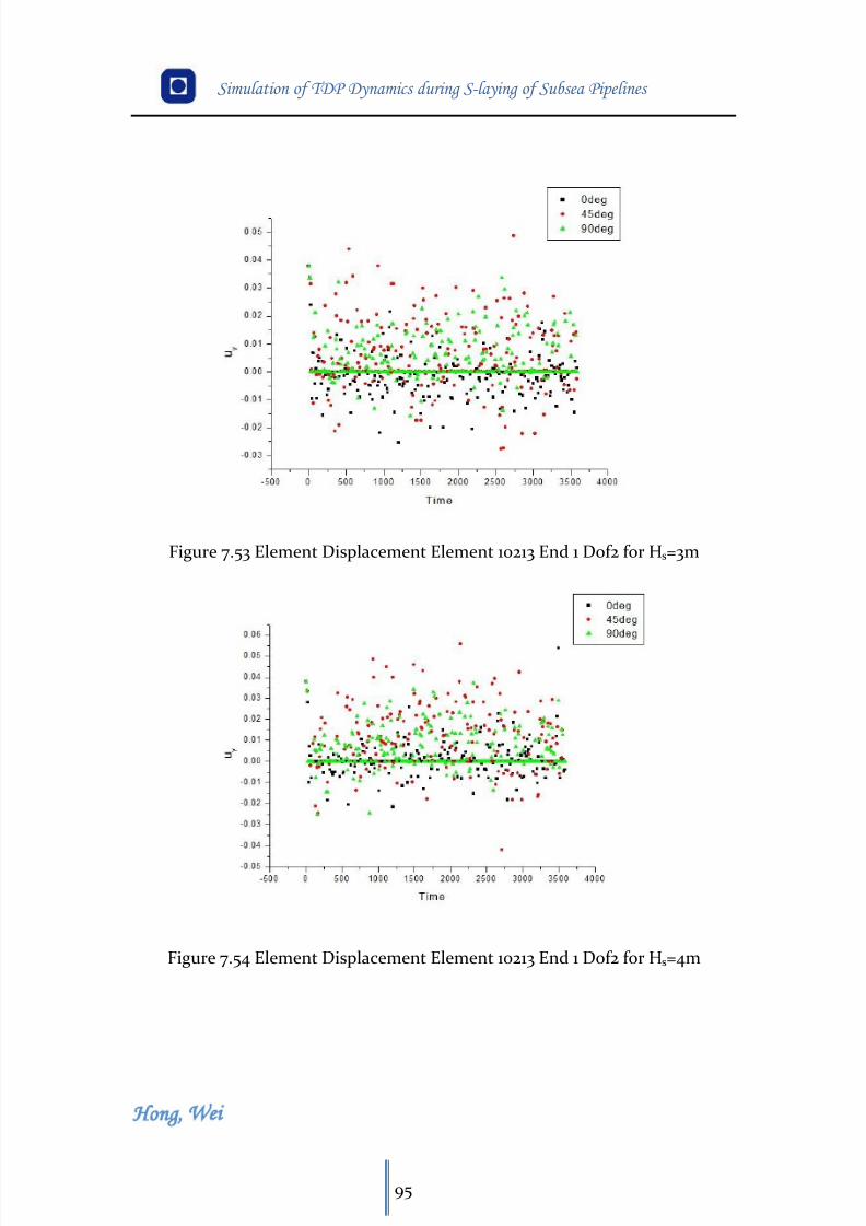
8/11/2019 Cañerías Offshore Instalación
http://slidepdf.com/reader/full/canerias-offshore-instalacion 106/157
Simulation of TDP Dynamics during S-laying of Subsea Pipelines
Hong Wei
95
Figure 7.53 Element Displacement Element 10213 End 1 Dof2 for Hs=3m
Figure 7.54 Element Displacement Element 10213 End 1 Dof2 for Hs=4m
8/11/2019 Cañerías Offshore Instalación
http://slidepdf.com/reader/full/canerias-offshore-instalacion 107/157
Simulation of TDP Dynamics during S-laying of Subsea Pipelines
Hong Wei
96
Chapter 8 Conclusion
The purpose of the thesis is to try to give some information about the
penetration of the pipeline during installation which may have large effect on
the intervention work and cost impact. Thus, the dynamics at the touch down
point (TDP) induced by 1st order motions from wave is of interest. It can
perhaps explain the larger penetration than predicted behavior.
The thesis work focus on dynamic simulation of pipelines using the computer
code. In order to get a comprehensive understanding of the problem, 4 sea
states combined with 3 wave direction angles which in total, 12 different
scenarios are studied in the thesis.
The wave direction angles have large effect on the vertical forces. It is veryobvious that the vertical force is the largest for wave direction 90 deg, second
for the 45 deg. As for 90 deg wave, the water particle velocity perpendicular to
the pipeline is the largest compared to the other two cases. Then the lift force
to the pipeline will be the largest. Thus the vertical force acts on the seabed will
smallest as it equals the submerged weight of the pipeline minus the lift force.
The wave direction angles have small effect on the transverse force and
displacement.
During the pipeline installation process, the pipeline keeps hitting and lifting
off the seabed, which gives the seabed cyclic loading to the seabed resulting in
larger penetration in the soil.
It is easy to understand that the more severe sea state, the more large response
of the pipelines which therefore larger response on the seabed.
8/11/2019 Cañerías Offshore Instalación
http://slidepdf.com/reader/full/canerias-offshore-instalacion 108/157
Simulation of TDP Dynamics during S-laying of Subsea Pipelines
Hong Wei
97
Recommendation for future work
This study is meant as an introduction investigation of the dynamics at the
touch down point induced by 1st order motions from waves. A lot of
simplifications have been made to easy the problem.
First, only the case for the installation using S-laying is studied here. It is also of
interest to studying more cases using different pipeline installation methods to
get a more overall understanding of the dynamics at the touch down point.
Second, a simple pipe-soil interaction model is used in this thesis. A pipeline
moving cyclically accumulates penetration, which therefore results in an
increased lateral soil resistance. So using the PONDUS pipe-soil interaction
model will give a more robust result.
8/11/2019 Cañerías Offshore Instalación
http://slidepdf.com/reader/full/canerias-offshore-instalacion 109/157
8/11/2019 Cañerías Offshore Instalación
http://slidepdf.com/reader/full/canerias-offshore-instalacion 110/157
Simulation of TDP Dynamics during S-laying of Subsea Pipelines
Hong Wei
99
Lambrakos, K. F. (1985): Marine Pipeline-Soil Friction Coefficients from In-Situ
Testing.
Langen, I. and Sigbjørnsson, R. (1979): Dynamisk Analyse av Konstruksjoner.Lennon, G.P. (1985): Wave-induced Forces on Pipelines buried in permeable
seabed.
Levold, E. (1990): Solid Mechanics and Material Models including Large
Deformations, PhD thesis, NTH.
Lyons, C.G., (1973): Soil Resistance to Lateral Sliding of Marine Pipeline.
Magda, W. (1999): Wave-induced Cyclic Pore-pressure Perturbation Effects in
Hydrodynamic Uplift Force Acting on Submarine Pipeline Buried on Seabed
Sediments.
Mattiason,K. (1983): On the Co-rotational Finite Element Formulation for Large
Deformation Problems. Technical Report Publication 83:1, Department of
Structural Mechanics, Chalmers University of Technology.
McMeeking, R.M., Marcal, P.V., and Rice, J.R. (1975): Finite Element
Formulations for Problems of Large Elastic-plastic deformation.
Morris, D.V., Webb, R.E., Dunlap, W.A. (1988): Self-Burial of Laterally Loaded
Offshore Pipelines in Weak Sediments.
Ole, H. and Torsten, S. (2008): A 3D Elasto-Plastic Spring Element for Pipe-Soil
Interaction Analysis.
Palmer, A.C., Steenfelt, J.S., Steensen Bach, J.O., and Jacobsen, V., (1988):
Lateral Resistance of Marine Pipelines on Sand.
Spierenburg, S.E.J. (1986): Wave-induced Pore Pressures around Submarine
Pipeline.
Svein Sævik (2008): SIMLA-Theory Manual. Marintek Report.
Svein Sævik, Ole David Økland, Gro Sagli Baarholm and Janne K.Ø. Gjøsteen
(2010): SIMLA Version 3.13.0 User manual.
Søreide, T.H (1989): Lecture Notes on Analysis of Non-Linear Structures.
Technical report, Norwegian Institute of Technology.
8/11/2019 Cañerías Offshore Instalación
http://slidepdf.com/reader/full/canerias-offshore-instalacion 111/157

8/11/2019 Cañerías Offshore Instalación
http://slidepdf.com/reader/full/canerias-offshore-instalacion 112/157
Simulation of TDP Dynamics during S-laying of Subsea Pipelines
Hong Wei
i
Appendix A
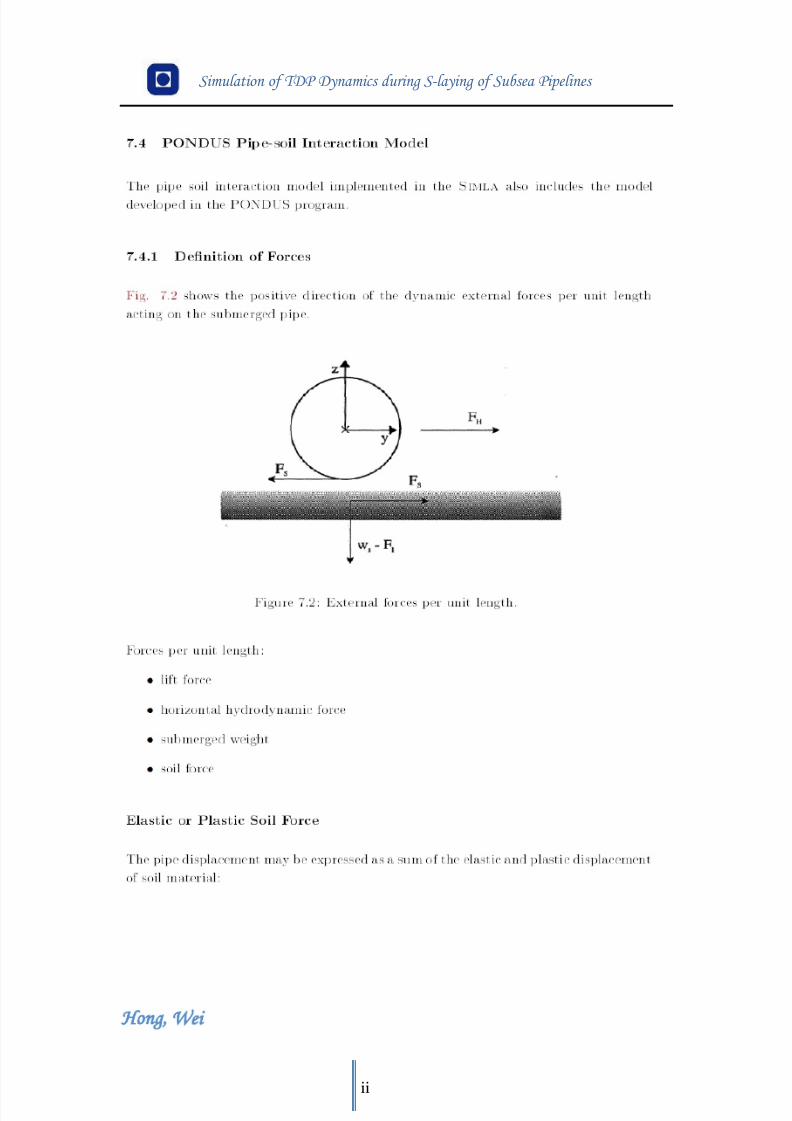
8/11/2019 Cañerías Offshore Instalación
http://slidepdf.com/reader/full/canerias-offshore-instalacion 113/157
Simulation of TDP Dynamics during S-laying of Subsea Pipelines
Hong Wei
ii
8/11/2019 Cañerías Offshore Instalación
http://slidepdf.com/reader/full/canerias-offshore-instalacion 114/157
Simulation of TDP Dynamics during S-laying of Subsea Pipelines
Hong Wei
iii
8/11/2019 Cañerías Offshore Instalación
http://slidepdf.com/reader/full/canerias-offshore-instalacion 115/157
Simulation of TDP Dynamics during S-laying of Subsea Pipelines
Hong Wei
iv
8/11/2019 Cañerías Offshore Instalación
http://slidepdf.com/reader/full/canerias-offshore-instalacion 116/157
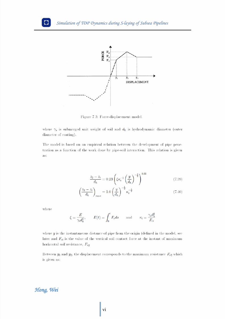
8/11/2019 Cañerías Offshore Instalación
http://slidepdf.com/reader/full/canerias-offshore-instalacion 117/157
Simulation of TDP Dynamics during S-laying of Subsea Pipelines
Hong Wei
vi
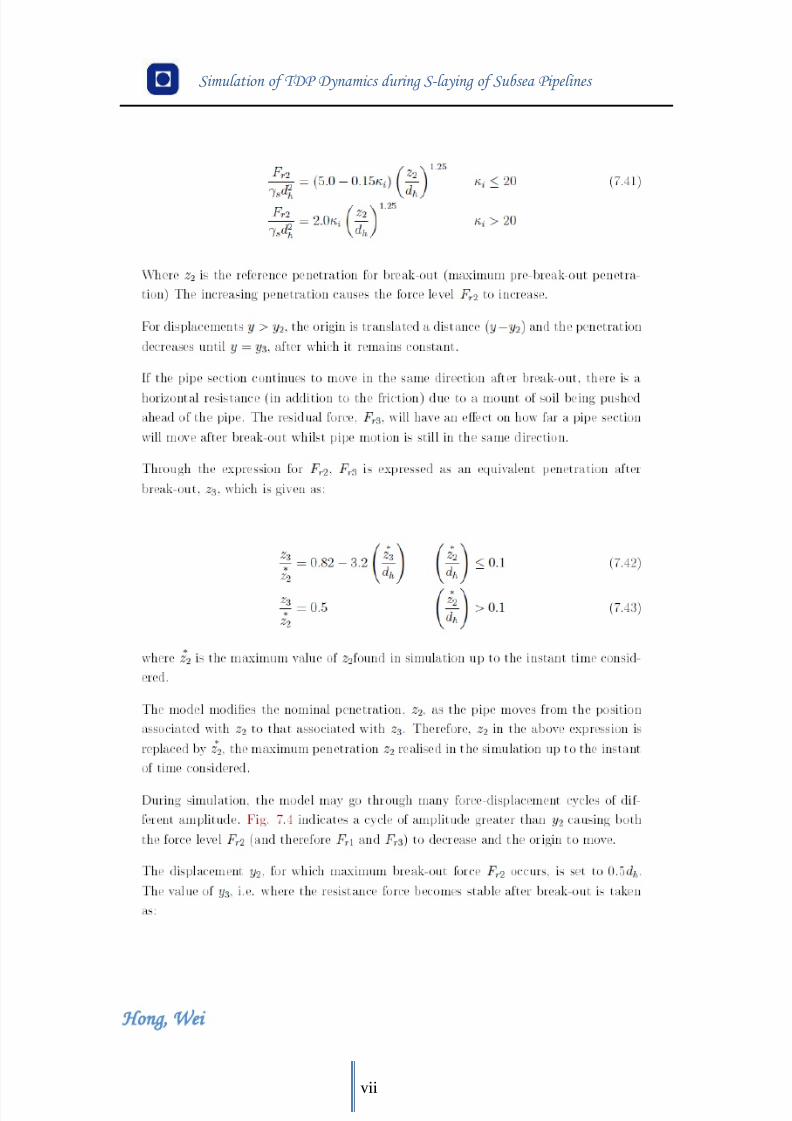
8/11/2019 Cañerías Offshore Instalación
http://slidepdf.com/reader/full/canerias-offshore-instalacion 118/157
Simulation of TDP Dynamics during S-laying of Subsea Pipelines
Hong Wei
vii
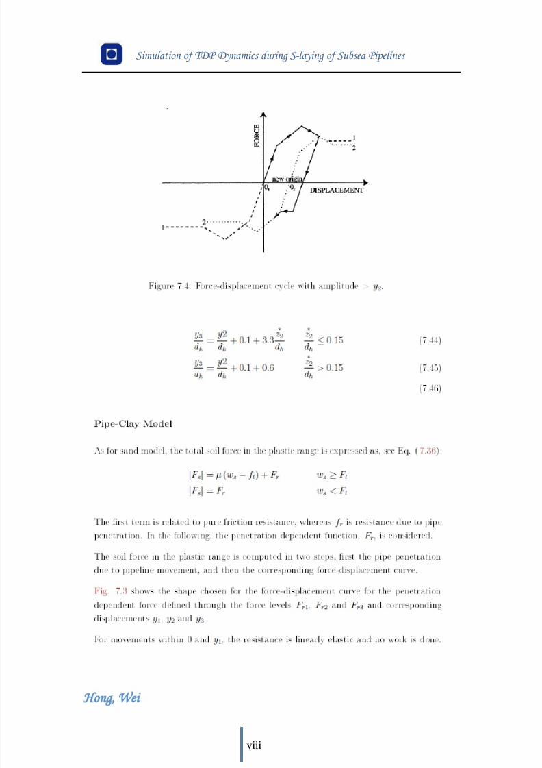
8/11/2019 Cañerías Offshore Instalación
http://slidepdf.com/reader/full/canerias-offshore-instalacion 119/157
Simulation of TDP Dynamics during S-laying of Subsea Pipelines
Hong Wei
viii
8/11/2019 Cañerías Offshore Instalación
http://slidepdf.com/reader/full/canerias-offshore-instalacion 120/157
Simulation of TDP Dynamics during S-laying of Subsea Pipelines
Hong Wei
ix
8/11/2019 Cañerías Offshore Instalación
http://slidepdf.com/reader/full/canerias-offshore-instalacion 121/157
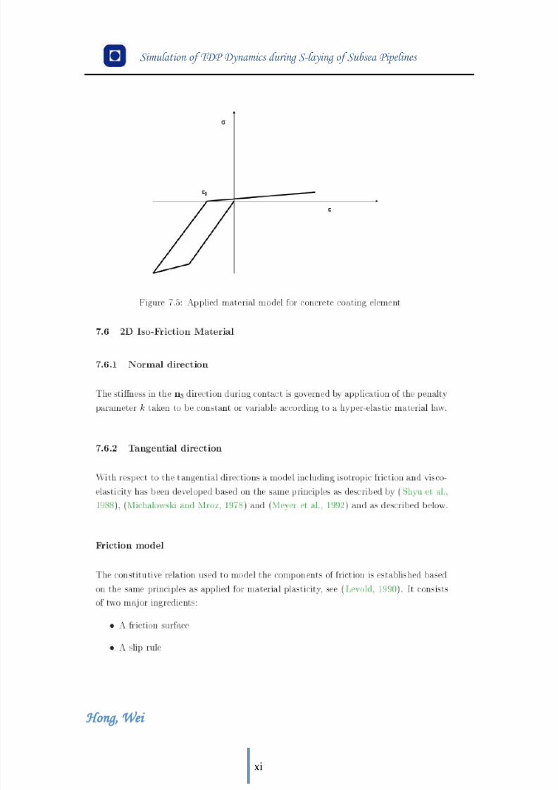
8/11/2019 Cañerías Offshore Instalación
http://slidepdf.com/reader/full/canerias-offshore-instalacion 122/157
Simulation of TDP Dynamics during S-laying of Subsea Pipelines
Hong Wei
xi
8/11/2019 Cañerías Offshore Instalación
http://slidepdf.com/reader/full/canerias-offshore-instalacion 123/157
Simulation of TDP Dynamics during S-laying of Subsea Pipelines
Hong Wei
xii
8/11/2019 Cañerías Offshore Instalación
http://slidepdf.com/reader/full/canerias-offshore-instalacion 124/157
Simulation of TDP Dynamics during S-laying of Subsea Pipelines
Hong Wei
xiii
8/11/2019 Cañerías Offshore Instalación
http://slidepdf.com/reader/full/canerias-offshore-instalacion 125/157
Simulation of TDP Dynamics during S-laying of Subsea Pipelines
Hong Wei
xiv
Appendix B
# Dynamical Analysis Model
HEAD This is a S-lay test example for a 32 " pipe at 200-300 m water depth
HEAD Irregular wave H=4m T = 10s - Elastic & elastoplastic material model - 500 pipe element
#
#-------------------------------------------------------------------
--------
# Control data:
#-------------------------------------------------------------------
--------
# maxit ndim isolvr npoint ipri conr gacc iproc
CONTROL 50 3 1 16 1 1e-5 9.81 restart 1
# imass alpha1 alpha2 alfa
DYNCONT 1 0.0 0.095 -0.05#
# visual results
#
VISRES integration 1 sigma-xx
# Dynamic Plots
DYNRES_N 1 3001 1
DYNRES_N 1 3001 2
DYNRES_N 1 3001 3
DYNRES_N 1 3001 4
DYNRES_N 1 3001 5
DYNRES_N 1 3001 6
DYNRES_N 1 224 1
DYNRES_N 1 224 2
DYNRES_E 2 2303 1 3
DYNRES_E 2 2304 1 3
DYNRES_E 2 2305 1 3
DYNRES_E 2 2306 1 3
DYNRES_E 2 2307 1 3
DYNRES_E 2 2308 1 3
8/11/2019 Cañerías Offshore Instalación
http://slidepdf.com/reader/full/canerias-offshore-instalacion 126/157
8/11/2019 Cañerías Offshore Instalación
http://slidepdf.com/reader/full/canerias-offshore-instalacion 127/157
Simulation of TDP Dynamics during S-laying of Subsea Pipelines
Hong Wei
xvi
DYNRES_E 2 10206 1 2
DYNRES_E 2 10207 1 2
DYNRES_E 2 10208 1 2
DYNRES_E 2 10209 1 2DYNRES_E 2 10210 1 2
DYNRES_E 2 10211 1 2
DYNRES_E 2 10212 1 2
DYNRES_E 2 10213 1 2
DYNRES_E 2 10214 1 2
DYNRES_E 2 10215 1 2
DYNRES_E 2 10216 1 2
DYNRES_E 2 10217 1 2
DYNRES_E 2 10218 1 2
DYNRES_E 2 10219 1 2
DYNRES_E 2 10220 1 2
DYNRES_E 2 10221 1 2
DYNRES_E 2 10222 1 2
DYNRES_E 2 10223 1 2
DYNRES_E 2 10224 1 2
##
DYNRES_E 2 10201 1 3
DYNRES_E 2 10202 1 3
DYNRES_E 2 10203 1 3DYNRES_E 2 10204 1 3
DYNRES_E 2 10205 1 3
DYNRES_E 2 10206 1 3
DYNRES_E 2 10207 1 3
DYNRES_E 2 10208 1 3
DYNRES_E 2 10209 1 3
DYNRES_E 2 10210 1 3
DYNRES_E 2 10211 1 3
DYNRES_E 2 10212 1 3
DYNRES_E 2 10213 1 3
DYNRES_E 2 10214 1 3
DYNRES_E 2 10215 1 3
DYNRES_E 2 10216 1 3
DYNRES_E 2 10217 1 3
DYNRES_E 2 10218 1 3
DYNRES_E 2 10219 1 3
DYNRES_E 2 10220 1 3
DYNRES_E 2 10221 1 3
DYNRES_E 2 10222 1 3
8/11/2019 Cañerías Offshore Instalación
http://slidepdf.com/reader/full/canerias-offshore-instalacion 128/157
Simulation of TDP Dynamics during S-laying of Subsea Pipelines
Hong Wei
xvii
DYNRES_E 2 10223 1 3
DYNRES_E 2 10224 1 3
##
ENVRES_N 1 1 501 1 1ENVRES_N 1 1 501 2 1
ENVRES_N 1 1 501 3 1
ENVRES_E 2 2301 2314 1 3 1
ENVRES_E 2 10001 10400 1 3 1
ENVRES_E 2 10001 10400 1 2 1
ENVRES_E 2 10001 10400 1 1 1
ENVRES_E 2 1 500 2 1 1
ENVRES_E 2 1 500 2 5 1
ENVRES_E 3 1 500 1 2 1
#
#-------------------------------------------------------------------
--------
# Units used (for correct display in plots)
#
# mass length time
UNITS 1.0e-3 1.0 1.0
#-----------------------------------------------------------
# Analysis time control:
#-----------------------------------------------------------# t dt dtvi dtdy dt0 type hla?
TIMECO 1.0 1.0 1.0 1.0 201.0 STATIC NOHLA
TIMECO 360.0 0.10 1.0 1.0 201.0 DYNAMIC NOHLA auto none all 20 5
1.0e-4
TIMECO 3600.0 0.10 10.0 1.0 201.0 DYNAMIC NOHLA auto none all 20
5 1.0e-4
#
#-------------------------------------------------------------------
--------
# Nocoor input
#-------------------------------------------------------------------
--------
#
# no x y z
NOCOOR coordinates 1 0 0 10
21 192.5983199 0 10
41 370.3978694 0 10
61 534.5357488 0 10
81 686.0616864 0 10
8/11/2019 Cañerías Offshore Instalación
http://slidepdf.com/reader/full/canerias-offshore-instalacion 129/157
Simulation of TDP Dynamics during S-laying of Subsea Pipelines
Hong Wei
xviii
101 825.9447521 0 10
121 955.0795549 0 10
141 1074.291964 0 10
161 1184.344392 0 10181 1285.940668 0 10
201 1379.730542 0 10
202 1384.226079 0 10
203 1388.703682 0 10
204 1393.163421 0 10
205 1397.605367 0 10
206 1402.029593 0 10
207 1406.436168 0 10
208 1410.825163 0 10
209 1415.196647 0 10
210 1419.550692 0 10
211 1423.887366 0 10
212 1428.206739 0 10
213 1432.50888 0 10
214 1436.793857 0 10
215 1441.061739 0 10
216 1445.312595 0 10
217 1449.546491 0 10
218 1453.763497 0 10219 1457.963678 0 10
220 1462.147103 0 10
221 1466.313838 0 10
222 1470.463949 0 10
223 1474.597504 0 10
224 1478.714568 0 10
225 1482.815207 0 10
226 1486.899486 0 10
227 1490.96747 0 10
228 1495.019226 0 10
229 1499.054817 0 10
230 1503.074308 0 10
231 1507.077763 0 10
232 1511.065246 0 10
233 1515.036821 0 10
234 1518.992551 0 10
235 1522.9325 0 10
236 1526.85673 0 10
237 1530.765305 0 10
8/11/2019 Cañerías Offshore Instalación
http://slidepdf.com/reader/full/canerias-offshore-instalacion 130/157
Simulation of TDP Dynamics during S-laying of Subsea Pipelines
Hong Wei
xix
238 1534.658286 0 10
239 1538.535736 0 10
240 1542.397717 0 10
241 1546.244291 0 10242 1550.075518 0 10
243 1553.891461 0 10
244 1557.69218 0 10
245 1561.477736 0 10
246 1565.248189 0 10
247 1569.0036 0 10
248 1572.744029 0 10
249 1576.469536 0 10
250 1580.180179 0 10
251 1583.876018 0 10
252 1587.557113 0 10
253 1591.223523 0 10
254 1594.875305 0 10
255 1598.512518 0 10
256 1602.13522 0 10
257 1605.74347 0 10
258 1609.337324 0 10
259 1612.916841 0 10
260 1616.482077 0 10261 1620.033089 0 10
262 1623.569935 0 10
263 1627.09267 0 10
264 1630.601351 0 10
265 1634.096035 0 10
266 1637.576776 0 10
267 1641.043631 0 10
268 1644.496654 0 10
269 1647.935902 0 10
270 1651.361429 0 10
271 1654.773289 0 10
272 1658.171538 0 10
273 1661.55623 0 10
274 1664.927418 0 10
275 1668.285157 0 10
276 1671.6295 0 10
277 1674.960501 0 10
278 1678.278212 0 10
279 1681.582688 0 10
8/11/2019 Cañerías Offshore Instalación
http://slidepdf.com/reader/full/canerias-offshore-instalacion 131/157
Simulation of TDP Dynamics during S-laying of Subsea Pipelines
Hong Wei
xx
280 1684.87398 0 10
281 1688.152142 0 10
282 1691.417225 0 10
283 1694.669282 0 10284 1697.908365 0 10
285 1701.134526 0 10
286 1704.347816 0 10
287 1707.548286 0 10
288 1710.735988 0 10
289 1713.910973 0 10
290 1717.07329 0 10
291 1720.222992 0 10
292 1723.360128 0 10
293 1726.484749 0 10
294 1729.596903 0 10
295 1732.696642 0 10
296 1735.784014 0 10
297 1738.859069 0 10
298 1741.921856 0 10
299 1744.972424 0 10
300 1748.010822 0 10
301 1751.037097 0 10
302 1754.0513 0 10303 1757.053477 0 10
304 1760.043677 0 10
305 1763.021948 0 10
306 1765.988337 0 10
307 1768.942891 0 10
308 1771.885658 0 10
309 1774.816685 0 10
310 1777.736018 0 10
311 1780.643705 0 10
312 1783.539791 0 10
313 1786.424323 0 10
314 1789.297348 0 10
315 1792.15891 0 10
316 1795.009057 0 10
317 1797.847832 0 10
318 1800.675282 0 10
319 1803.491452 0 10
320 1806.296387 0 10
321 1809.090132 0 10

8/11/2019 Cañerías Offshore Instalación
http://slidepdf.com/reader/full/canerias-offshore-instalacion 132/157
Simulation of TDP Dynamics during S-laying of Subsea Pipelines
Hong Wei
xxi
322 1811.87273 0 10
323 1814.644228 0 10
324 1817.404668 0 10
325 1820.154096 0 10326 1822.892555 0 10
327 1825.620089 0 10
328 1828.336741 0 10
329 1831.042555 0 10
330 1833.737574 0 10
331 1836.421842 0 10
332 1839.0954 0 10
333 1841.758292 0 10
334 1844.410561 0 10
335 1847.052248 0 10
336 1849.683396 0 10
337 1852.304047 0 10
338 1854.914243 0 10
339 1857.514026 0 10
340 1860.103436 0 10
341 1862.682517 0 10
342 1865.251307 0 10
343 1867.80985 0 10
344 1870.358185 0 10345 1872.896354 0 10
346 1875.424397 0 10
347 1877.942353 0 10
348 1880.450265 0 10
349 1882.948171 0 10
350 1885.436112 0 10
351 1887.914127 0 10
352 1890.382256 0 10
353 1892.840538 0 10
354 1895.289013 0 10
355 1897.727719 0 10
356 1900.156697 0 10
357 1902.575984 0 10
358 1904.985619 0 10
359 1907.38564 0 10
360 1909.776087 0 10
361 1912.156997 0 10
362 1914.528409 0 10
363 1916.89036 0 10
8/11/2019 Cañerías Offshore Instalación
http://slidepdf.com/reader/full/canerias-offshore-instalacion 133/157
Simulation of TDP Dynamics during S-laying of Subsea Pipelines
Hong Wei
xxii
364 1919.242887 0 10
365 1921.586029 0 10
366 1923.919824 0 10
367 1926.244307 0 10368 1928.559517 0 10
369 1930.86549 0 10
370 1933.162264 0 10
371 1935.449874 0 10
372 1937.728358 0 10
373 1939.997752 0 10
374 1942.258092 0 10
375 1944.509415 0 10
376 1946.751756 0 10
377 1948.985151 0 10
378 1951.209636 0 10
379 1953.425246 0 10
380 1955.632017 0 10
381 1957.829984 0 10
382 1960.019182 0 10
383 1962.199646 0 10
384 1964.371412 0 10
385 1966.534513 0 10
386 1968.688984 0 10387 1970.83486 0 10
388 1972.972175 0 10
389 1975.100963 0 10
390 1977.221258 0 10
391 1979.333094 0 10
392 1981.436505 0 10
393 1983.531525 0 10
394 1985.618186 0 10
395 1987.696523 0 10
396 1989.766568 0 10
397 1991.828354 0 10
398 1993.881915 0 10
399 1995.927284 0 10
400 1997.964492 0 10
401 1999.993573 0 10
501 2200.000000 0 10.0000
#
NOCOOR coordinates 3001 2289.469 0 5.0
NOCOOR coordinates 2101 16357 10385 0
8/11/2019 Cañerías Offshore Instalación
http://slidepdf.com/reader/full/canerias-offshore-instalacion 134/157
8/11/2019 Cañerías Offshore Instalación
http://slidepdf.com/reader/full/canerias-offshore-instalacion 135/157
Simulation of TDP Dynamics during S-laying of Subsea Pipelines
Hong Wei
xxiv
REPEAT 400 1 1
#
# group elty material ID n1 n2 n3 n4
ELCON ormpipe2 pipe33 pipemat2 401 401 402# n j k
REPEAT 100 1 1
# Lay-vessel
# group elty material ID n1 n2
ELCON vessel1 spring137 vessel1 3000 3001 501
#
# name of surface ID n1
ELCON seabed cont126 cosurf1 10001 1
# n j k
REPEAT 400 1 1
#
#
# The stinger section
ELCON ormcontact cont164 roller1 2301 3001
ELCON ormcontact1 cont164 roller2 2302 3001
ELCON ormcontact2 cont164 roller3 2303 3001
ELCON ormcontact3 cont164 roller4 2304 3001
ELCON ormcontact4 cont164 roller5 2305 3001
ELCON ormcontact5 cont164 roller6 2306 3001ELCON ormcontact6 cont164 roller7 2307 3001
ELCON ormcontact7 cont164 roller8 2308 3001
ELCON ormcontact8 cont164 roller9 2309 3001
ELCON ormcontact9 cont164 roller10 2310 3001
ELCON ormcontact10 cont164 roller11 2311 3001
ELCON ormcontact11 cont164 roller12 2312 3001
# n j
REPEAT 3 1 0
#
ELCON ormcontact12 cont164 roller13 2401 3001
# n j
REPEAT 4 1 0
#
ELCON sea1 sea150 seamat 2101 2101 2102 2113 2112
REPEAT 10 1 1
repeat 10 10 11
#
# Elecc data:
#------------------------------------------------------------------
8/11/2019 Cañerías Offshore Instalación
http://slidepdf.com/reader/full/canerias-offshore-instalacion 136/157
Simulation of TDP Dynamics during S-laying of Subsea Pipelines
Hong Wei
xxv
#
# type elno end ex ey ez fi dx1 dy1
dz1 dx2 dy2 dz2
ELECC stinger 2301 1 -89.469 0 4.252 0 0 -1 0 0 1 0
ELECC stinger 2302 1 -110.410041 0 3.058111827 -0.113900467 0 -1
0 0 1 0
ELECC stinger 2303 1 -130.4379832 0 -0.360522377 -0.224227216 0
-1 0 0 1 0
ELECC stinger 2304 1 -139.2163505 0 -2.590866573 -0.273389145 0
-1 0 0 1 0
ELECC stinger 2305 1 -149.7034056 0 -5.871840641 -0.333035425 0
-1 0 0 1 0
ELECC stinger 2306 1 -159.634299 0 -9.630899746 -0.390673873 0
-1 0 0 1 0
ELECC stinger 2307 1 -168.4635771 0 -13.54082696 -0.443087862 0
-1 0 0 1 0
ELECC stinger 2308 1 -177.329431 0 -18.04524037 -0.497066699 0
-1 0 0 1 0
ELECC stinger 2309 1 -187.1788443 0 -23.78993046 -0.558960837 0
-1 0 0 1 0
ELECC stinger 2310 1 -195.3690509 0 -29.22208808 -0.612306666 0
-1 0 0 1 0ELECC stinger 2311 1 -202.1900777 0 -34.25104409 -0.658304683 0
-1 0 0 1 0
ELECC stinger 2312 1 -208.0500466 0 -38.97753767 -0.699167567 0
-1 0 0 1 0
ELECC stinger 2313 1 -213.7204751 0 -43.94717772 -0.740092451 0
-1 0 0 1 0
ELECC stinger 2314 1 -219.2000795 0 -49.16175439 -0.781149162 0 -1
0 0 1 0
ELECC stinger 2401 1 -110.410041 0 3.058111827 -0.113900467 0
-0.75048 0 0 -0.75048 1.5
ELECC stinger 2402 1 -110.410041 0 3.058111827 -0.113900467 0
0.75048 0 0 0.75048 1.5
ELECC stinger 2403 1 -187.1788443 0 -23.78993046 -0.558960837 0
-0.75048 0 0 -0.75048 1.5
ELECC stinger 2404 1 -187.1788443 0 -23.78993046 -0.558960837 0
0.75048 0 0 0.75048 1.5
ELECC beam 3000 1 -89.469 0 4.999
#------------------------------------------------------------------
#
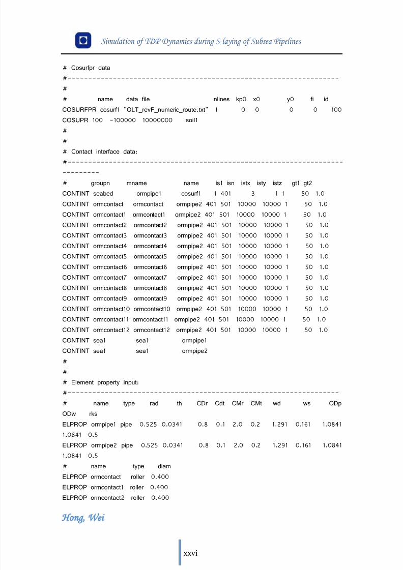
8/11/2019 Cañerías Offshore Instalación
http://slidepdf.com/reader/full/canerias-offshore-instalacion 137/157
Simulation of TDP Dynamics during S-laying of Subsea Pipelines
Hong Wei
xxvi
# Cosurfpr data
#------------------------------------------------------------------
#
# name data file nlines kp0 x0 y0 fi idCOSURFPR cosurf1 "OLT_revF_numeric_route.txt" 1 0 0 0 0 100
COSUPR 100 -100000 10000000 soil1
#
#
# Contact interface data:
#-------------------------------------------------------------------
---------
# groupn mname name is1 isn istx isty istz gt1 gt2
CONTINT seabed ormpipe1 cosurf1 1 401 3 1 1 50 1.0
CONTINT ormcontact ormcontact ormpipe2 401 501 10000 10000 1 50 1.0
CONTINT ormcontact1 ormcontact1 ormpipe2 401 501 10000 10000 1 50 1.0
CONTINT ormcontact2 ormcontact2 ormpipe2 401 501 10000 10000 1 50 1.0
CONTINT ormcontact3 ormcontact3 ormpipe2 401 501 10000 10000 1 50 1.0
CONTINT ormcontact4 ormcontact4 ormpipe2 401 501 10000 10000 1 50 1.0
CONTINT ormcontact5 ormcontact5 ormpipe2 401 501 10000 10000 1 50 1.0
CONTINT ormcontact6 ormcontact6 ormpipe2 401 501 10000 10000 1 50 1.0
CONTINT ormcontact7 ormcontact7 ormpipe2 401 501 10000 10000 1 50 1.0
CONTINT ormcontact8 ormcontact8 ormpipe2 401 501 10000 10000 1 50 1.0
CONTINT ormcontact9 ormcontact9 ormpipe2 401 501 10000 10000 1 50 1.0CONTINT ormcontact10 ormcontact10 ormpipe2 401 501 10000 10000 1 50 1.0
CONTINT ormcontact11 ormcontact11 ormpipe2 401 501 10000 10000 1 50 1.0
CONTINT ormcontact12 ormcontact12 ormpipe2 401 501 10000 10000 1 50 1.0
CONTINT sea1 sea1 ormpipe1
CONTINT sea1 sea1 ormpipe2
#
#
# Element property input:
#------------------------------------------------------------------
# name type rad th CDr Cdt CMr CMt wd ws ODp
ODw rks
ELPROP ormpipe1 pipe 0.525 0.0341 0.8 0.1 2.0 0.2 1.291 0.161 1.0841
1.0841 0.5
ELPROP ormpipe2 pipe 0.525 0.0341 0.8 0.1 2.0 0.2 1.291 0.161 1.0841
1.0841 0.5
# name type diam
ELPROP ormcontact roller 0.400
ELPROP ormcontact1 roller 0.400
ELPROP ormcontact2 roller 0.400
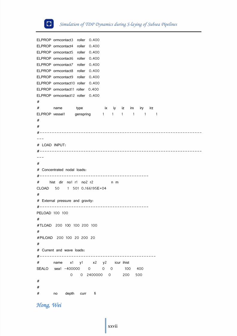
8/11/2019 Cañerías Offshore Instalación
http://slidepdf.com/reader/full/canerias-offshore-instalacion 138/157
Simulation of TDP Dynamics during S-laying of Subsea Pipelines
Hong Wei
xxvii
ELPROP ormcontact3 roller 0.400
ELPROP ormcontact4 roller 0.400
ELPROP ormcontact5 roller 0.400
ELPROP ormcontact6 roller 0.400ELPROP ormcontact7 roller 0.400
ELPROP ormcontact8 roller 0.400
ELPROP ormcontact9 roller 0.400
ELPROP ormcontact10 roller 0.400
ELPROP ormcontact11 roller 0.400
ELPROP ormcontact12 roller 0.400
#
# name type ix iy iz irx iry irz
ELPROP vessel1 genspring 1 1 1 1 1 1
#
#
#-------------------------------------------------------------------
---
# LOAD INPUT:
#-------------------------------------------------------------------
---
#
# Concentrated nodal loads:
#---------------------------------------------# hist dir no1 r1 no2 r2 n m
CLOAD 50 1 501 0.166195E+04
#
# External pressure and gravity:
#---------------------------------------------
PELOAD 100 100
#
#TLOAD 200 100 100 200 100
#
#PILOAD 200 100 20 200 20
#
# Current and wave loads:
#------------------------------------------------
# name x1 y1 x2 y2 icur ihist
SEALO sea1 -400000 0 0 0 100 400
0 0 2400000 0 200 500
#
#
# no depth curr fi
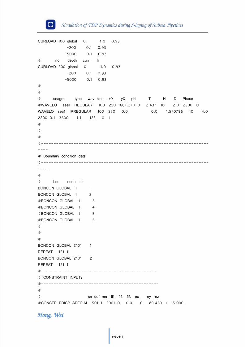
8/11/2019 Cañerías Offshore Instalación
http://slidepdf.com/reader/full/canerias-offshore-instalacion 139/157
Simulation of TDP Dynamics during S-laying of Subsea Pipelines
Hong Wei
xxviii
CURLOAD 100 global 0 1.0 0.93
-200 0.1 0.93
-5000 0.1 0.93
# no depth curr fiCURLOAD 200 global 0 1.0 0.93
-200 0.1 0.93
-5000 0.1 0.93
#
#
# seagrp type wav hist x0 y0 phi T H D Phase
#WAVELO sea1 REGULAR 100 250 1667.270 0 2.437 10 2.0 2200 0
WAVELO sea1 IRREGULAR 100 250 0.0 0.0 1.570796 10 4.0
2200 0.1 3600 1.1 125 0 1
#
#
#
#-------------------------------------------------------------------
----
# Boundary condition data
#-------------------------------------------------------------------
----
#
# Loc node dirBONCON GLOBAL 1 1
BONCON GLOBAL 1 2
#BONCON GLOBAL 1 3
#BONCON GLOBAL 1 4
#BONCON GLOBAL 1 5
#BONCON GLOBAL 1 6
#
#
#
BONCON GLOBAL 2101 1
REPEAT 121 1
BONCON GLOBAL 2101 2
REPEAT 121 1
#-----------------------------------------------
# CONSTRAINT INPUT:
#-----------------------------------------------
#
# sn dof mn fi1 fi2 fi3 ex ey ez
#CONSTR PDISP SPECIAL 501 1 3001 0 0.0 0 -89.469 0 5.000
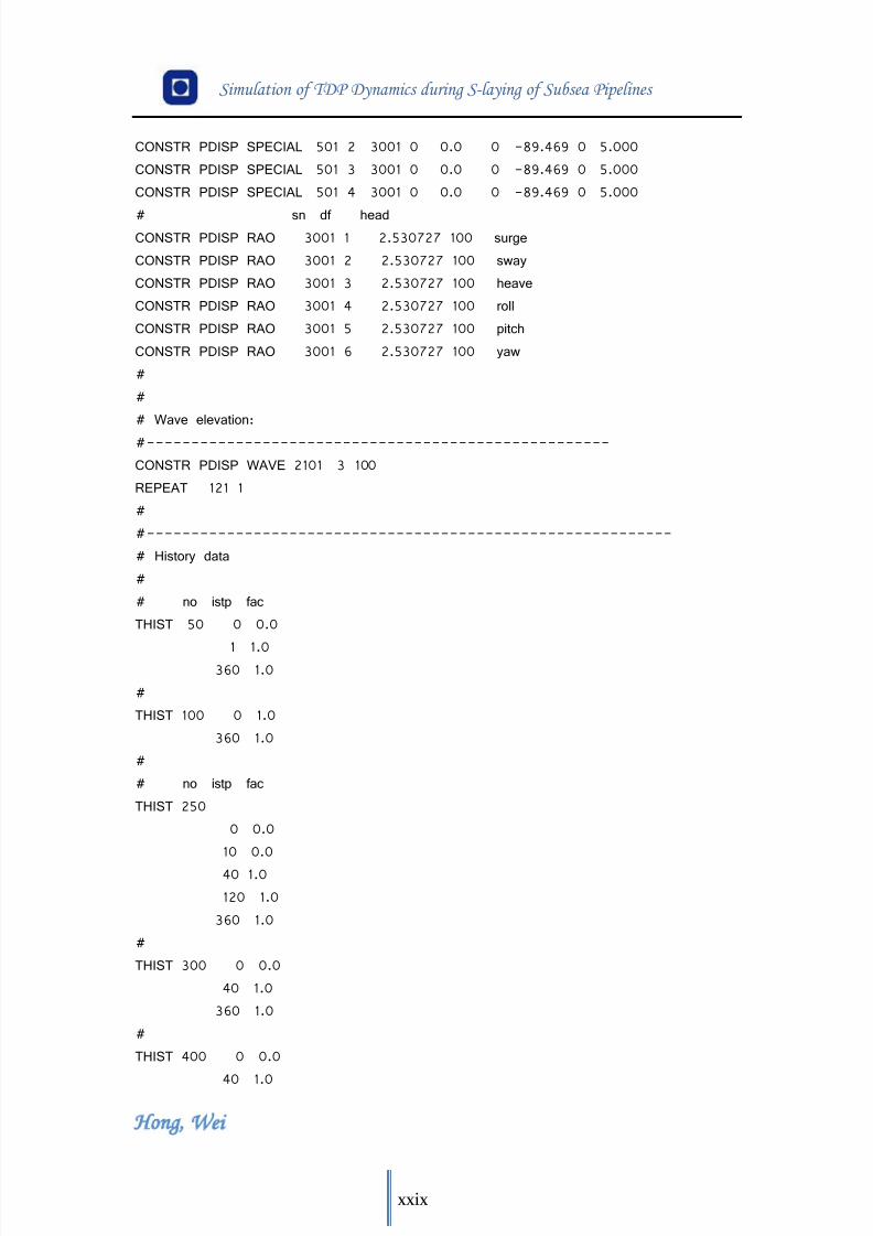
8/11/2019 Cañerías Offshore Instalación
http://slidepdf.com/reader/full/canerias-offshore-instalacion 140/157
Simulation of TDP Dynamics during S-laying of Subsea Pipelines
Hong Wei
xxix
CONSTR PDISP SPECIAL 501 2 3001 0 0.0 0 -89.469 0 5.000
CONSTR PDISP SPECIAL 501 3 3001 0 0.0 0 -89.469 0 5.000
CONSTR PDISP SPECIAL 501 4 3001 0 0.0 0 -89.469 0 5.000
# sn df headCONSTR PDISP RAO 3001 1 2.530727 100 surge
CONSTR PDISP RAO 3001 2 2.530727 100 sway
CONSTR PDISP RAO 3001 3 2.530727 100 heave
CONSTR PDISP RAO 3001 4 2.530727 100 roll
CONSTR PDISP RAO 3001 5 2.530727 100 pitch
CONSTR PDISP RAO 3001 6 2.530727 100 yaw
#
#
# Wave elevation:
#----------------------------------------------------
CONSTR PDISP WAVE 2101 3 100
REPEAT 121 1
#
#-----------------------------------------------------------
# History data
#
# no istp fac
THIST 50 0 0.0
1 1.0360 1.0
#
THIST 100 0 1.0
360 1.0
#
# no istp fac
THIST 250
0 0.0
10 0.0
40 1.0
120 1.0
360 1.0
#
THIST 300 0 0.0
40 1.0
360 1.0
#
THIST 400 0 0.0
40 1.0
8/11/2019 Cañerías Offshore Instalación
http://slidepdf.com/reader/full/canerias-offshore-instalacion 141/157
Simulation of TDP Dynamics during S-laying of Subsea Pipelines
Hong Wei
xxx
360 1.0
THIST 500 0 0.0
40 1.0
360 1.0THIST 999 0 0.0
360 0.0
#
#
#-------------------------------------------------------------------
-----------
# Material data:
#-------------------------------------------------------------------
-----------
#
# name type poiss talfa tecond heatc beta ea
MATERIAL pipemat1 linear 0.3 1.17e-5 50 800 0 2.249e7
eiy eiz git em gm
3.10e6 3.10e6 2.39e6 2e8 8e7
# name type alfa poiss ro talfa tecondheatc eps sigma
#
MATERIAL pipemat2 elastoplastic 1 0.3 7.850 1.17e-5 50 800 0 0
1.691E-03
3.50E+050.005 4.50E+05
9.980E-02
8.35E+05
# name type density
MATERIAL seamat sea 1000e-3
# name type rmyx rmyy xname yname zname
MATERIAL soil1 contact 0.5 1.0 soilx soily soilz
MATERIAL soil2 contact 0.5 1.0 soilx soily soilz2
MATERIAL roller1 contact 0.3 0.3 soilx soily soilz3
MATERIAL roller2 contact 0.3 0.3 soilx soily soilz4
MATERIAL roller3 contact 0.3 0.3 soilx soily soilz5
MATERIAL roller4 contact 0.3 0.3 soilx soily soilz6
MATERIAL roller5 contact 0.3 0.3 soilx soily soilz7
MATERIAL roller6 contact 0.3 0.3 soilx soily soilz8
MATERIAL roller7 contact 0.3 0.3 soilx soily soilz9
MATERIAL roller8 contact 0.3 0.3 soilx soily soilz10
MATERIAL roller9 contact 0.3 0.3 soilx soily soilz11
MATERIAL roller10 contact 0.3 0.3 soilx soily soilz12
MATERIAL roller11 contact 0.3 0.3 soilx soily soilz13
8/11/2019 Cañerías Offshore Instalación
http://slidepdf.com/reader/full/canerias-offshore-instalacion 142/157
Simulation of TDP Dynamics during S-laying of Subsea Pipelines
Hong Wei
xxxi
MATERIAL roller12 contact 0.3 0.3 soilx soily soilz14
MATERIAL roller13 contact 0.3 0.3 soilx soily soilz15
# name type alfa eps sig
MATERIAL soilx epcurve 1 0 00.005 1
100.00 10
# name type eps sig
MATERIAL soily epcurve 1 0 0
0.10 1
100.00 2
# name type eps sig
MATERIAL soilz hycurve -10000 -10000000
10000 10000000
#
# name type eps sig
MATERIAL soilz2 hycurve -10000 -10000000
10000 10000000
#
# name type eps sig
MATERIAL soilz3 hycurve -10000 -240000000
10000 240000000
MATERIAL soilz4 hycurve -10000 -220000000
10000 220000000MATERIAL soilz5 hycurve -10000 -200000000
10000 200000000
MATERIAL soilz6 hycurve -10000 -170000000
10000 170000000
MATERIAL soilz7 hycurve -10000 -142000000
10000 142000000
MATERIAL soilz8 hycurve -10000 -116000000
10000 116000000
MATERIAL soilz9 hycurve -10000 -82000000
10000 82000000
MATERIAL soilz10 hycurve -10000 -58000000
10000 58000000
MATERIAL soilz11 hycurve -10000 -48000000
10000 48000000
MATERIAL soilz12 hycurve -10000 -40000000
10000 40000000
MATERIAL soilz13 hycurve -10000 -30000000
10000 30000000
MATERIAL soilz14 hycurve -10000 -20000000
8/11/2019 Cañerías Offshore Instalación
http://slidepdf.com/reader/full/canerias-offshore-instalacion 143/157
Simulation of TDP Dynamics during S-laying of Subsea Pipelines
Hong Wei
xxxii
10000 20000000
MATERIAL soilz15 hycurve -10000 -200000000
10000 200000000
## name type apr1 spr2 spr3 spr4 spr5 spr6
MATERIAL vessel1 genspring surgesp1 yawsp heavesp rollsp pitchsp swaysp
# Tensioner
MATERIAL surgesp epcurve 1
0.00 0.0
1.00 50.0
23.00 200.0
MATERIAL surgesp1 hycurve -10000 -50000
-24.00 -40000
-23.00 -200
-1.00 -50
1.00 50
23.00 200
24.00 40000
10000 50000
MATERIAL surgesp2 hycurve -1000 0
1000 0
MATERIAL yawsp hycurve -1000 0
1000 0MATERIAL heavesp hycurve -1000 0
1000 0
MATERIAL rollsp hycurve -1000 0
1000 0
MATERIAL pitchsp hycurve -1000 0
1000 0
MATERIAL swaysp hycurve -1000 0
1000 0
#--------------------------------------------------
# RAO definitions:
#--------------------------------------------------
#--------------------------------------------------
# RAO definitions:
#--------------------------------------------------
RAOPROP surge DEF 0 1.57 3.14 4.71 6.28 surge1 surge2 surge3 surge4 surge5
RAOPROP sway DEF 0 1.57 3.14 4.71 6.28 sway1 sway2 sway3 sway4 sway5
RAOPROP heave DEF 0 1.57 3.14 4.71 6.28 heave1 heave2 heave3 heave4 heave5
RAOPROP roll DEF 0 1.57 3.14 4.71 6.28 roll1 roll2 roll3 roll4 roll5
RAOPROP pitch DEF 0 1.57 3.14 4.71 6.28 pitch1 pitch2 pitch3 pitch4 pitch5
8/11/2019 Cañerías Offshore Instalación
http://slidepdf.com/reader/full/canerias-offshore-instalacion 144/157
Simulation of TDP Dynamics during S-laying of Subsea Pipelines
Hong Wei
xxxiii
RAOPROP yaw DEF 0 1.57 3.14 4.71 6.28 yaw1 yaw2 yaw3 yaw4 yaw5
#
RAOPROP surge1 CURVE 0 0 0.000000000
0.314159265 1.1908 3.1293753490.34906585 1.0798 3.127630020
0.369599136 1.0253 3.127630020
0.392699082 0.9693 3.124139361
0.41887902 0.909 3.122394032
0.448798951 0.8391 3.125884690
0.483321947 0.7541 3.127630020
0.502654825 0.7029 3.132866007
0.523598776 0.6435 -3.136356666
0.54636394 0.5734 -3.111922056
0.571198664 0.4888 -3.061307508
0.598398601 0.3833 -2.954842424
0.628318531 0.2414 -2.696533694
0.661387927 0.0802 -1.642354826
0.698131701 0.1581 0.322885912
0.785398163 0.1889 0.895353906
0.897597901 0.1167 -1.162389282
1.047197551 0.0337 -1.956514091
1.256637061 0.0581 0.497418837
1.570796327 0.0143 -2.651155134
RAOPROP surge2 CURVE 0 0 0.000000000
0.314159265 0 0.000000000
0.34906585 0 0.000000000
0.369599136 0 0.000000000
0.392699082 0 0.000000000
0.41887902 0 0.000000000
0.448798951 0 0.000000000
0.483321947 0 0.000000000
0.502654825 0 0.000000000
0.523598776 0 0.000000000
0.54636394 0 0.000000000
0.571198664 0 0.000000000
0.598398601 0 0.000000000
0.628318531 0 0.000000000
0.661387927 0 0.000000000
0.698131701 0 0.000000000
0.785398163 0 0.000000000
0.897597901 0 0.000000000
8/11/2019 Cañerías Offshore Instalación
http://slidepdf.com/reader/full/canerias-offshore-instalacion 145/157
Simulation of TDP Dynamics during S-laying of Subsea Pipelines
Hong Wei
xxxiv
1.047197551 0 0.000000000
1.256637061 0 0.000000000
1.570796327 0 0.000000000
RAOPROP surge3 CURVE 0 0 0.000000000
0.314159265 -1.1908 3.129375349
0.34906585 -1.0798 3.12763002
0.369599136 -1.0253 3.12763002
0.392699082 -0.9693 3.124139361
0.41887902 -0.909 3.122394032
0.448798951 -0.8391 3.12588469
0.483321947 -0.7541 3.12763002
0.502654825 -0.7029 3.132866007
0.523598776 -0.6435 -3.136356666
0.54636394 -0.5734 -3.111922056
0.571198664 -0.4888 -3.061307508
0.598398601 -0.3833 -2.954842424
0.628318531 -0.2414 -2.696533694
0.661387927 -0.0802 -1.642354826
0.698131701 -0.1581 0.322885912
0.785398163 -0.1889 0.895353906
0.897597901 -0.1167 -1.162389282
1.047197551 -0.0337 -1.9565140911.256637061 -0.0581 0.497418837
1.570796327 -0.0143 -2.651155134
RAOPROP surge4 CURVE 0 0 0.000000000
0.314159265 0 0.000000000
0.34906585 0 0.000000000
0.369599136 0 0.000000000
0.392699082 0 0.000000000
0.41887902 0 0.000000000
0.448798951 0 0.000000000
0.483321947 0 0.000000000
0.502654825 0 0.000000000
0.523598776 0 0.000000000
0.54636394 0 0.000000000
0.571198664 0 0.000000000
0.598398601 0 0.000000000
0.628318531 0 0.000000000
0.661387927 0 0.000000000
0.698131701 0 0.000000000
8/11/2019 Cañerías Offshore Instalación
http://slidepdf.com/reader/full/canerias-offshore-instalacion 146/157
Simulation of TDP Dynamics during S-laying of Subsea Pipelines
Hong Wei
xxxv
0.785398163 0 0.000000000
0.897597901 0 0.000000000
1.047197551 0 0.000000000
1.256637061 0 0.0000000001.570796327 0 0.000000000
RAOPROP surge5 CURVE 0 0 0.000000000
0.314159265 1.1908 3.129375349
0.34906585 1.0798 3.127630020
0.369599136 1.0253 3.127630020
0.392699082 0.9693 3.124139361
0.41887902 0.909 3.122394032
0.448798951 0.8391 3.125884690
0.483321947 0.7541 3.127630020
0.502654825 0.7029 3.132866007
0.523598776 0.6435 -3.136356666
0.54636394 0.5734 -3.111922056
0.571198664 0.4888 -3.061307508
0.598398601 0.3833 -2.954842424
0.628318531 0.2414 -2.696533694
0.661387927 0.0802 -1.642354826
0.698131701 0.1581 0.322885912
0.785398163 0.1889 0.8953539060.897597901 0.1167 -1.162389282
1.047197551 0.0337 -1.956514091
1.256637061 0.0581 0.497418837
1.570796327 0.0143 -2.651155134
RAOPROP sway1 CURVE 0 0 0.000000000
0.314159265 0 0.000000000
0.34906585 0 0.000000000
0.369599136 0 0.000000000
0.392699082 0 0.000000000
0.41887902 0 0.000000000
0.448798951 0 0.000000000
0.483321947 0 0.000000000
0.502654825 0 0.000000000
0.523598776 0 0.000000000
0.54636394 0 0.000000000
0.571198664 0 0.000000000
0.598398601 0 0.000000000
8/11/2019 Cañerías Offshore Instalación
http://slidepdf.com/reader/full/canerias-offshore-instalacion 147/157
Simulation of TDP Dynamics during S-laying of Subsea Pipelines
Hong Wei
xxxvi
0.628318531 0 0.000000000
0.661387927 0 0.000000000
0.698131701 0 0.000000000
0.785398163 0 0.0000000000.897597901 0 0.000000000
1.047197551 0 0.000000000
1.256637061 0 0.000000000
1.570796327 0 0
RAOPROP sway2 CURVE 0 0 0.000000000
0.314159265 1.1908 3.129375349
0.34906585 1.0798 3.127630020
0.369599136 1.0253 3.127630020
0.392699082 0.9693 3.124139361
0.41887902 0.909 3.122394032
0.448798951 0.8391 3.125884690
0.483321947 0.7541 3.127630020
0.502654825 0.7029 3.132866007
0.523598776 0.6435 -3.136356666
0.54636394 0.5734 -3.111922056
0.571198664 0.4888 -3.061307508
0.598398601 0.3833 -2.954842424
0.628318531 0.2414 -2.6965336940.661387927 0.0802 -1.642354826
0.698131701 0.1581 0.322885912
0.785398163 0.1889 0.895353906
0.897597901 0.1167 -1.162389282
1.047197551 0.0337 -1.956514091
1.256637061 0.0581 0.497418837
1.570796327 0.0143 -2.651155134
RAOPROP sway3 CURVE 0 0 0.000000000
0.314159265 0 0.000000000
0.34906585 0 0.000000000
0.369599136 0 0.000000000
0.392699082 0 0.000000000
0.41887902 0 0.000000000
0.448798951 0 0.000000000
0.483321947 0 0.000000000
0.502654825 0 0.000000000
0.523598776 0 0.000000000
0.54636394 0 0.000000000
8/11/2019 Cañerías Offshore Instalación
http://slidepdf.com/reader/full/canerias-offshore-instalacion 148/157
Simulation of TDP Dynamics during S-laying of Subsea Pipelines
Hong Wei
xxxvii
0.571198664 0 0.000000000
0.598398601 0 0.000000000
0.628318531 0 0.000000000
0.661387927 0 0.0000000000.698131701 0 0.000000000
0.785398163 0 0.000000000
0.897597901 0 0.000000000
1.047197551 0 0.000000000
1.256637061 0 0.000000000
1.570796327 0 0
RAOPROP sway4 CURVE 0 0 0.000000000
0.314159265 -1.1908 3.129375349
0.34906585 -1.0798 3.12763002
0.369599136 -1.0253 3.12763002
0.392699082 -0.9693 3.124139361
0.41887902 -0.909 3.122394032
0.448798951 -0.8391 3.12588469
0.483321947 -0.7541 3.12763002
0.502654825 -0.7029 3.132866007
0.523598776 -0.6435 -3.136356666
0.54636394 -0.5734 -3.111922056
0.571198664 -0.4888 -3.0613075080.598398601 -0.3833 -2.954842424
0.628318531 -0.2414 -2.696533694
0.661387927 -0.0802 -1.642354826
0.698131701 -0.1581 0.322885912
0.785398163 -0.1889 0.895353906
0.897597901 -0.1167 -1.162389282
1.047197551 -0.0337 -1.956514091
1.256637061 -0.0581 0.497418837
1.570796327 -0.0143 -2.651155134
RAOPROP sway5 CURVE 0 0 0.000000000
0.314159265 0 0.000000000
0.34906585 0 0.000000000
0.369599136 0 0.000000000
0.392699082 0 0.000000000
0.41887902 0 0.000000000
0.448798951 0 0.000000000
0.483321947 0 0.000000000
0.502654825 0 0.000000000
8/11/2019 Cañerías Offshore Instalación
http://slidepdf.com/reader/full/canerias-offshore-instalacion 149/157
Simulation of TDP Dynamics during S-laying of Subsea Pipelines
Hong Wei
xxxviii
0.523598776 0 0.000000000
0.54636394 0 0.000000000
0.571198664 0 0.000000000
0.598398601 0 0.0000000000.628318531 0 0.000000000
0.661387927 0 0.000000000
0.698131701 0 0.000000000
0.785398163 0 0.000000000
0.897597901 0 0.000000000
1.047197551 0 0.000000000
1.256637061 0 0.000000000
1.570796327 0 0
RAOPROP heave1 CURVE 0 0 0
0.314159265 1.0639 0.829031395
0.34906585 1.0692 0.753982237
0.369599136 1.0767 0.706858347
0.392699082 1.0844 0.654498469
0.41887902 1.0906 0.596902604
0.448798951 1.0907 0.53581608
0.483321947 1.0688 0.464257581
0.502654825 1.0455 0.4241150080.523598776 1.01 0.380481777
0.54636394 0.963 0.333357887
0.571198664 0.9081 0.277507351
0.598398601 0.8551 0.240855437
0.628318531 0.7643 0.298451302
0.661387927 0.5216 0.521853446
0.698131701 0.1095 0.773180859
0.785398163 0.2618 -1.987930018
0.897597901 0.0802 1.628392192
1.047197551 0.1258 1.256637061
1.256637061 0.1161 -2.605776573
1.570796327 0.0291 -1.436405974
RAOPROP heave2 CURVE 0 0 0
0.314159265 1.0639 0.829031395
0.34906585 1.0692 0.753982237
0.369599136 1.0767 0.706858347
0.392699082 1.0844 0.654498469
0.41887902 1.0906 0.596902604
8/11/2019 Cañerías Offshore Instalación
http://slidepdf.com/reader/full/canerias-offshore-instalacion 150/157
Simulation of TDP Dynamics during S-laying of Subsea Pipelines
Hong Wei
xxxix
0.448798951 1.0907 0.53581608
0.483321947 1.0688 0.464257581
0.502654825 1.0455 0.424115008
0.523598776 1.01 0.3804817770.54636394 0.963 0.333357887
0.571198664 0.9081 0.277507351
0.598398601 0.8551 0.240855437
0.628318531 0.7643 0.298451302
0.661387927 0.5216 0.521853446
0.698131701 0.1095 0.773180859
0.785398163 0.2618 -1.987930018
0.897597901 0.0802 1.628392192
1.047197551 0.1258 1.256637061
1.256637061 0.1161 -2.605776573
1.570796327 0.0291 -1.436405974
RAOPROP heave3 CURVE 0 0 0
0.314159265 1.0639 0.829031395
0.34906585 1.0692 0.753982237
0.369599136 1.0767 0.706858347
0.392699082 1.0844 0.654498469
0.41887902 1.0906 0.596902604
0.448798951 1.0907 0.535816080.483321947 1.0688 0.464257581
0.502654825 1.0455 0.424115008
0.523598776 1.01 0.380481777
0.54636394 0.963 0.333357887
0.571198664 0.9081 0.277507351
0.598398601 0.8551 0.240855437
0.628318531 0.7643 0.298451302
0.661387927 0.5216 0.521853446
0.698131701 0.1095 0.773180859
0.785398163 0.2618 -1.987930018
0.897597901 0.0802 1.628392192
1.047197551 0.1258 1.256637061
1.256637061 0.1161 -2.605776573
1.570796327 0.0291 -1.436405974
RAOPROP heave4 CURVE 0 0 0
0.314159265 1.0639 0.829031395
0.34906585 1.0692 0.753982237
0.369599136 1.0767 0.706858347
8/11/2019 Cañerías Offshore Instalación
http://slidepdf.com/reader/full/canerias-offshore-instalacion 151/157
Simulation of TDP Dynamics during S-laying of Subsea Pipelines
Hong Wei
xl
0.392699082 1.0844 0.654498469
0.41887902 1.0906 0.596902604
0.448798951 1.0907 0.53581608
0.483321947 1.0688 0.4642575810.502654825 1.0455 0.424115008
0.523598776 1.01 0.380481777
0.54636394 0.963 0.333357887
0.571198664 0.9081 0.277507351
0.598398601 0.8551 0.240855437
0.628318531 0.7643 0.298451302
0.661387927 0.5216 0.521853446
0.698131701 0.1095 0.773180859
0.785398163 0.2618 -1.987930018
0.897597901 0.0802 1.628392192
1.047197551 0.1258 1.256637061
1.256637061 0.1161 -2.605776573
1.570796327 0.0291 -1.436405974
RAOPROP heave5 CURVE 0 0 0
0.314159265 1.0639 0.829031395
0.34906585 1.0692 0.753982237
0.369599136 1.0767 0.706858347
0.392699082 1.0844 0.6544984690.41887902 1.0906 0.596902604
0.448798951 1.0907 0.53581608
0.483321947 1.0688 0.464257581
0.502654825 1.0455 0.424115008
0.523598776 1.01 0.380481777
0.54636394 0.963 0.333357887
0.571198664 0.9081 0.277507351
0.598398601 0.8551 0.240855437
0.628318531 0.7643 0.298451302
0.661387927 0.5216 0.521853446
0.698131701 0.1095 0.773180859
0.785398163 0.2618 -1.987930018
0.897597901 0.0802 1.628392192
1.047197551 0.1258 1.256637061
1.256637061 0.1161 -2.605776573
1.570796327 0.0291 -1.436405974
RAOPROP roll1 CURVE 0 0 0.000000000
8/11/2019 Cañerías Offshore Instalación
http://slidepdf.com/reader/full/canerias-offshore-instalacion 152/157
Simulation of TDP Dynamics during S-laying of Subsea Pipelines
Hong Wei
xli
0.314159265 0 0.000000000
0.34906585 0 0.000000000
0.369599136 0 0.000000000
0.392699082 0 0.0000000000.41887902 0 0.000000000
0.448798951 0 0.000000000
0.483321947 0 0.000000000
0.502654825 0 0.000000000
0.523598776 0 0.000000000
0.54636394 0 0.000000000
0.571198664 0 0.000000000
0.598398601 0 0.000000000
0.628318531 0 0.000000000
0.661387927 0 0.000000000
0.698131701 0 0.000000000
0.785398163 0 0.000000000
0.897597901 0 0.000000000
1.047197551 0 0.000000000
1.256637061 0 0.000000000
1.570796327 0 0
RAOPROP roll2 CURVE 0 0 0.000000000
0.314159265 0.00996583 -0.0279252680.34906585 0.0108926 -0.027925268
0.369599136 0.011477285 -0.026179939
0.392699082 0.012126548 -0.02443461
0.41887902 0.012821189 -0.02443461
0.448798951 0.013494886 -0.013962634
0.483321947 0.014060372 -0.005235988
0.502654825 0.014254104 0.003490659
0.523598776 0.014327408 0.019198622
0.54636394 0.014241887 0.04712389
0.571198664 0.013894566 0.097738438
0.598398601 0.013158037 0.193731547
0.628318531 0.011445869 0.39618974
0.661387927 0.007897615 0.799360797
0.698131701 0.003136357 1.736602606
0.785398163 0.004256858 -2.331759881
0.897597901 0.000949459 1.123992038
1.047197551 0.001469567 1.052433539
1.256637061 0.001350885 -2.686061719
1.570796327 0.000439823 -1.466076572
8/11/2019 Cañerías Offshore Instalación
http://slidepdf.com/reader/full/canerias-offshore-instalacion 153/157
8/11/2019 Cañerías Offshore Instalación
http://slidepdf.com/reader/full/canerias-offshore-instalacion 154/157
Simulation of TDP Dynamics during S-laying of Subsea Pipelines
Hong Wei
xliii
1.256637061 -0.001350885 -2.686061719
1.570796327 -0.000439823 -1.466076572
RAOPROP roll5 CURVE 0 0 0.0000000000.314159265 0 0.000000000
0.34906585 0 0.000000000
0.369599136 0 0.000000000
0.392699082 0 0.000000000
0.41887902 0 0.000000000
0.448798951 0 0.000000000
0.483321947 0 0.000000000
0.502654825 0 0.000000000
0.523598776 0 0.000000000
0.54636394 0 0.000000000
0.571198664 0 0.000000000
0.598398601 0 0.000000000
0.628318531 0 0.000000000
0.661387927 0 0.000000000
0.698131701 0 0.000000000
0.785398163 0 0.000000000
0.897597901 0 0.000000000
1.047197551 0 0.000000000
1.256637061 0 0.0000000001.570796327 0 0
RAOPROP pitch1 CURVE 0 0 0.000000000
0.314159265 0.00996583 -0.027925268
0.34906585 0.0108926 -0.027925268
0.369599136 0.011477285 -0.026179939
0.392699082 0.012126548 -0.02443461
0.41887902 0.012821189 -0.02443461
0.448798951 0.013494886 -0.013962634
0.483321947 0.014060372 -0.005235988
0.502654825 0.014254104 0.003490659
0.523598776 0.014327408 0.019198622
0.54636394 0.014241887 0.04712389
0.571198664 0.013894566 0.097738438
0.598398601 0.013158037 0.193731547
0.628318531 0.011445869 0.39618974
0.661387927 0.007897615 0.799360797
0.698131701 0.003136357 1.736602606
8/11/2019 Cañerías Offshore Instalación
http://slidepdf.com/reader/full/canerias-offshore-instalacion 155/157
8/11/2019 Cañerías Offshore Instalación
http://slidepdf.com/reader/full/canerias-offshore-instalacion 156/157
Simulation of TDP Dynamics during S-laying of Subsea Pipelines
Hong Wei
xlv
0.661387927 -0.007897615 0.799360797
0.698131701 -0.003136357 1.736602606
0.785398163 -0.004256858 -2.331759881
0.897597901 -0.000949459 1.1239920381.047197551 -0.001469567 1.052433539
1.256637061 -0.001350885 -2.686061719
1.570796327 -0.000439823 -1.466076572
RAOPROP pitch4 CURVE 0 0 0.000000000
0.314159265 0 0.000000000
0.34906585 0 0.000000000
0.369599136 0 0.000000000
0.392699082 0 0.000000000
0.41887902 0 0.000000000
0.448798951 0 0.000000000
0.483321947 0 0.000000000
0.502654825 0 0.000000000
0.523598776 0 0.000000000
0.54636394 0 0.000000000
0.571198664 0 0.000000000
0.598398601 0 0.000000000
0.628318531 0 0.000000000
0.661387927 0 0.0000000000.698131701 0 0.000000000
0.785398163 0 0.000000000
0.897597901 0 0.000000000
1.047197551 0 0.000000000
1.256637061 0 0.000000000
1.570796327 0 0
RAOPROP pitch5 CURVE 0 0 0.000000000
0.314159265 0.00996583 -0.027925268
0.34906585 0.0108926 -0.027925268
0.369599136 0.011477285 -0.026179939
0.392699082 0.012126548 -0.02443461
0.41887902 0.012821189 -0.02443461
0.448798951 0.013494886 -0.013962634
0.483321947 0.014060372 -0.005235988
0.502654825 0.014254104 0.003490659
0.523598776 0.014327408 0.019198622
0.54636394 0.014241887 0.04712389
0.571198664 0.013894566 0.097738438
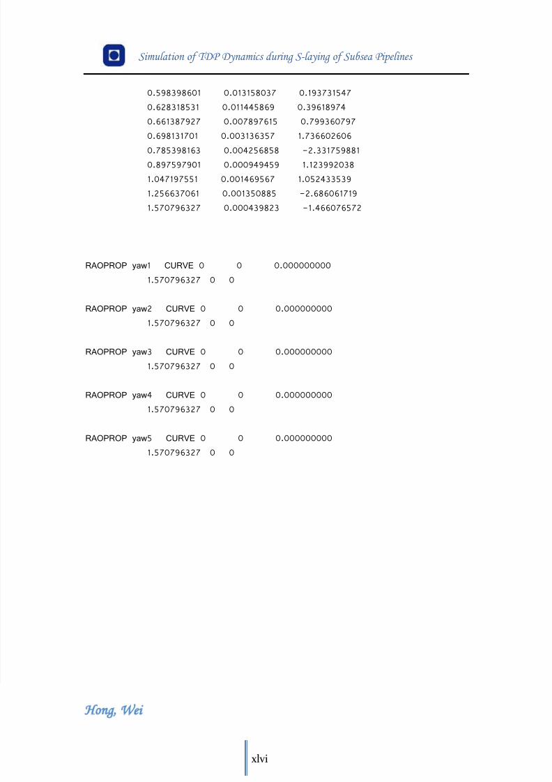
8/11/2019 Cañerías Offshore Instalación
http://slidepdf.com/reader/full/canerias-offshore-instalacion 157/157
Simulation of TDP Dynamics during S-laying of Subsea Pipelines
0.598398601 0.013158037 0.193731547
0.628318531 0.011445869 0.39618974
0.661387927 0.007897615 0.799360797
0.698131701 0.003136357 1.7366026060.785398163 0.004256858 -2.331759881
0.897597901 0.000949459 1.123992038
1.047197551 0.001469567 1.052433539
1.256637061 0.001350885 -2.686061719
1.570796327 0.000439823 -1.466076572
RAOPROP yaw1 CURVE 0 0 0.000000000
1.570796327 0 0
RAOPROP yaw2 CURVE 0 0 0.000000000
1.570796327 0 0
RAOPROP yaw3 CURVE 0 0 0.000000000
1.570796327 0 0
RAOPROP yaw4 CURVE 0 0 0.000000000

![Informe Offshore[1]](https://static.fdocuments.es/doc/165x107/5695d4911a28ab9b02a1eddf/informe-offshore1.jpg)