Concepción y Diseño de un Sistema de Medición del Perfil...
124
Concepción y Diseño de un Sistema de Medición del Perfil de Velocidades y del Nivel del Agua en un Canal de Pruebas NOVIEMBRE 2017 Álvaro Quiles García DIRECTOR DEL TRABAJO FIN DE GRADO: Emilio Migoya Valor Álvaro Quiles García TRABAJO FIN DE GRADO PARA LA OBTENCIÓN DEL TÍTULO DE GRADUADO EN INGENIERÍA EN TECNOLOGÍAS INDUSTRIALES
Transcript of Concepción y Diseño de un Sistema de Medición del Perfil...

Concepción y Diseño de un Sistema de Medición del Perfil de Velocidades y del Nivel del Agua en un Canal de Pruebas
NOVIEMBRE 2017
Álvaro Quiles García
DIRECTOR DEL TRABAJO FIN DE GRADO:
Emilio Migoya Valor
Álv
aro
Qu
ile
s G
arc
ía
TRABAJO FIN DE GRADO PARA
LA OBTENCIÓN DEL TÍTULO DE
GRADUADO EN INGENIERÍA EN
TECNOLOGÍAS INDUSTRIALES

Universidad Politécnica de Madrid
Escuela Técnica Superior de Ingenieros Industriales
TRABAJO DE FIN DE GRADO
GRADO EN INGENIERÍA EN TECNOLOGÍAS INDUSTRIALES
Concepción y Diseño de un Sistema de Medición del Perfil de
Velocidades y Nivel de Agua para una Plataforma de Prueba de Canal
Álvaro Quiles García
Número de matrícula: 13370
Tutor: Emilio Migoya Valor
Noviembre 2017
Madrid

II

III
Tabla de Contenido Del Resumen en Español
1 INTRODUCCIÓN Y MOTIVACIÓN ............................................................................. V
2 ESTADO DEL ARTE .................................................................................................. IX
3 DISEÑO DEL SISTEMA DE MEDICIÓN................................................................. XI
4 DISEÑO DE LA ESTRUCTURA DE LA TURBINA .............................................. XVII
5 ELECCIÓN DE RESISTENCIAS DE LA TURBINA SOBRE EL FLUJO ........... XIX
6 CONCLUSIONES Y TRABAJOS FUTUROS ............................................................ XXI

IV

V
1 Introducción y Motivación
El presente Trabajo de Fin de Grado forma parte de un proyecto de mayores dimensiones
realizado en la universidad TU Darmstadt, dicho proyecto se basa en la modelización y
simulación de una turbina mareomotriz mediante un canal de agua diseñado por
(Hernandez, 2013) y mejorado por (Lehr, 2014), el objetivo del proyecto es calcular la
eficiencia energética de la aplicación de una turbina mareomotriz real.
Más concretamente, el presente TFG se va a centrar en la concepción y diseño de un
sistema de medición que sea capaz de medir parámetros que a posteriori serán necesarios
para futuros trabajos dentro del proyecto anteriormente mencionado.
Dentro del departamento de fluidos (FST) de la universidad TU Darmstadt se ha diseñado
un modelo para calcular el coeficiente de operatividad 𝐶𝑝 para canales rectangulares
hidráulicos con obstrucción completa tanto de altura como de anchura (Pelz, 2011).
A diferencia de las plantas hidráulicas convencionales, las turbinas mareomotrices se
caracterizan por no tener una obstrucción completa. El presente trabajo estudiará turbinas
con obstrucción completa de anchura, pero no de altura de manera que se consiga un flujo
de derivación vertical.
El mayor problema a la hora de diseñar un sistema de medición para una turbina
mareomotriz es la influencia de la superficie libre alrededor de la turbina, debido a la
presencia de una cascada, salto de altura, la cual genera una diferencia de energía estática.
El modelo analítico en el cual está basado el presente TFG se realizó mediante la
conservación de la energía, la ecuación de continuidad y el principio de impulso lineal.
El sistema de medición diseñado debe ser capaz de medir la velocidad del flujo, la línea
media y la anchura del tubo de corriente producido por la turbina y la altimetría del nivel del
agua del canal.
Otra parte importante de este trabajo consiste en el diseño de un sistema que pueda mejorar
el manejo de la turbina. Esto significa encontrar un sistema más automático que el actual, el
cual a la hora de modificar el tipo de turbina o cambiar la posición de la turbina, está basado
en un sistema de tornillos, siendo este muy incómodo a la hora de trabajar. En definitiva, se
busca una estructura más manejable.
El experimento va a consistir en la modelización de una turbina real, donde se va a usar un
plato perforado en vez de una turbina normal, debido al tamaño del canal de agua. Este
plato perforado tendrá una anchura igual a la del canal de agua, lo que implica una
obstrucción horizontal completa mientras que su altura será variable.
VI
La elección de los platos perforados como “turbina” se debe principalmente a dos razones:
En primer lugar, debido a que representa un flujo de derivación vertical, el cual es
característico de las turbinas mareomotrices. La segunda razón es la no importancia del tipo
de energía que se disipa ya que el resultado final a nivel de cálculo va a ser el mismo. En el
presente caso, los platos perforados van a disipar calor en ved de energía mecánica.
La Figura 1 representa el modelo con el que se va a trabajar:
Figura 1: Simulación Experimental del Flujo
Como se puede observar, existen cinco puntos de interés a lo largo del canal, (1), (+), (-), (2)
y (3). Este trabajo se centrará en la zona comprendida entre los puntos (+) y (2), ya que es
el área de conflicto por la presencia de la cascada. Aun siendo cierto que este trabajo se
centra en la zona entre los puntos (+) y (2), también se estudiará la zona entre (1) y (+).
Otra consecuencia relevante del uso de un flujo de derivación vertical reside en la diferencia
de velocidades entre el agua que pasa por el plato perforado y el que pasa por el flujo de
derivación (𝑢20 > 𝑢2𝑖). Esto es interesante ya que el caudal volumétrico que pasa por el
plato perforado se conserva hasta la zona de mezcla, como se puede apreciar en la Figura
1.
El canal de pruebas usado para la experimentación es el mostrado en las Figuras 2 y 3, se
puede definir como un circuito cerrado debido a que el agua es la misma todo el rato, dicha
agua viene de un tanque situado justo abajo del canal.
VII
Figura 2: Canal de Pruebas 3D
Figura 3: Canal de Pruebas 2D
La entrada del canal está fabricada de acero inoxidable y posee un filtro de agujeros
redondeados, mediante el cual se consigue un desarrollo progresivo de la capa límite y un
mejor perfil de velocidades en el canal. El canal de pruebas también posee un
homogeneizador y un control del caudal volumétrico en la entrada.
Otro aspecto que considerar es el material del cristal del canal, vidrio acrílico, el cual fue
escogido por (Hernandez, 2013) debido a su transparencia. Este material puede ser muy útil
a la hora de usar técnicas de medición de carácter óptimo como lo son PIV o PTV, estas
técnicas serán importantes a la hora de la elección final del sistema de medición
Antes de empezar con el estudio del diseño del sistema de medición es necesario estudiar
la variación de ciertos parámetros.

VIII
El caudal volumétrico máximo con el que la bomba puede trabajar es de 82 m3 /h. El número
de Froude, 𝐹𝑟 =𝑄
𝑏√𝑔·ℎ3 considerado va a depender de la zona del canal de pruebas, donde
Q es el caudal, b es la anchura y h es la altura de agua en el punto estudiado.
En la entrada se buscará un número de Froude comprendido entre los valores 0 y 0.3,
mientras que en la salida estará comprendido entre 0 y 0.5. El número máximo de Froude al
que se podrá enfrentar el canal de pruebas es de 1.4 en la zona de la cascada. Con lo que
se puede afirmar que el flujo de agua es subcrítico en todo el canal menos en la cascada
donde es supercrítico.
Sabiendo el caudal y el número de Froude, se calcula el rango de velocidades en el que se
puede trabajar, mediante la siguiente expresión:
𝑢 = ( 𝐹𝑟√𝑔𝑄
𝑏 )2/3
Donde se obtienen velocidades en el canal entre 0.2 y 1.3 m/s. Es conveniente tener en
cuenta que los perfiles de velocidad justo después de la turbina no son homogéneos. Por
tanto, como se estudió previamente en (Nieschlag, 2016), ver sección 2.2, es necesario
multiplicar por un factor de 1.3. Resultando en que la velocidad máxima del canal
previamente explicado será de 1.7 m/s.
El número de Reynolds también es necesario calcularlo, y se puede calcular mediante la
siguiente expresión para canales abiertos con forma rectangular (Pelz, 2011).
𝑅𝑒 =4 · 𝑢𝑜 · ℎ0
(1 + 2ℎ0𝑏
)𝜈
Se obtiene un número de Reynolds a lo largo del canal de 𝑅𝑒 (𝐹𝑟 = [0.1, 1.4]) = [7.3 ·
104, 2.4 · 105]. Con lo que se obtiene un flujo de carácter turbulento en el canal de pruebas.
Otros cálculos de menor relevancia han sido calculados en la sección 2.2.

IX
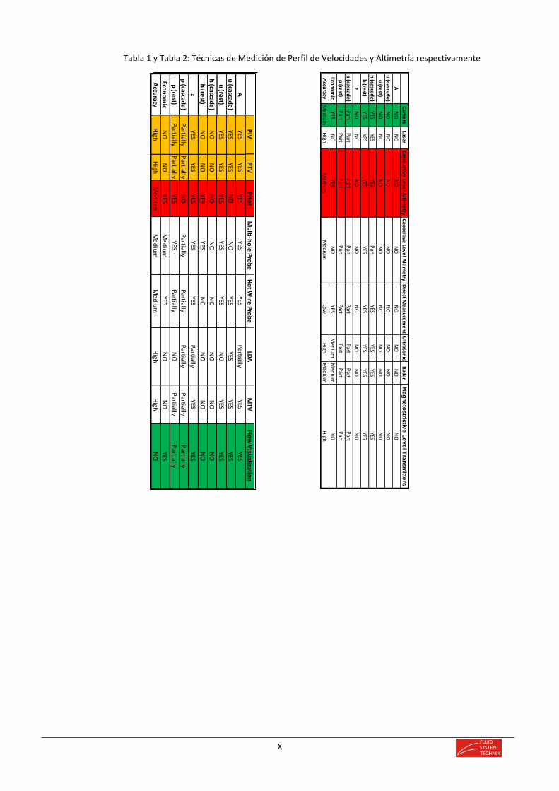
2 Estado del Arte
La primera parte del trabajo se centra en el estudio completo de las diferentes técnicas de
medición existentes a día de hoy en el mercado. Más concretamente en las principales
técnicas de medición para velocidades de flujo y para la altimetría de este. Este apartado
esta detallado en la sección 4.
Para la medición de la velocidad se han encontrado ocho posibles técnicas: PIV, PTV, Tubo
de Pitot, Sondas de Múltiples Agujeros, Sondas de Alambre Caliente, Laser Doppler
Anemometry, Molecular Tagging Velocimetry y Visualización del Flujo. Estas técnicas están
ampliamente explicadas en la sección 4.1. En la tabla 2 se puede observar una comparativa
entre ellas.
Para la medición del nivel del fluido en el canal de pruebas se han encontrado también ocho
posibles técnicas: Cámara de Alta resolución, Láser, Conductive Level Altimetry, Capacitive
Level Altimetry, Medida Directa, Ultrasonido, Radar y Magnetostrictive Level Transmitters.
Estas técnicas están ampliamente explicadas en la sección 4.2. En la tabla 3 se puede
observar una comparativa entre ellas.
Tras realizar el estudio de los posibles métodos se tendrá que buscar combinaciones entre
las diferentes técnicas para satisfacer todos los objetivos que tiene el diseño del sistema de
medición. Estos son los comentados en la sección 3., medición de la velocidad del flujo, la
línea media, la anchura del tubo de corriente producido por la turbina y la altura del flujo en
el canal de pruebas.
X
Tabla 1 y Tabla 2: Técnicas de Medición de Perfil de Velocidades y Altimetría respectivamente
PIV
P
TVP
itot
Mu
lti-ho
le P
rob
eH
ot W
ire P
rob
eLD
AM
TVFlo
w V
isualizatio
n
AYES
YESYES
YESYES
Partially
YESYES
u (cascad
e)
YESYES
NO
NO
YESYES
YESYES
u (re
st)YES
YESYES
YESYES
NO
YESYES
h (cascad
e)
NO
NO
NO
NO
NO
NO
NO
NO
h (re
st) N
ON
OYES
YESN
ON
ON
ON
O
zYES
YESYES
YESYES
Partially
YESYES
p (cascad
e)
Partially
Partially
NO
Partially
Partially
Partially
Partially
Partially
p (re
st)P
artiallyP
artiallyYES
YESP
artiallyN
OP
artiallyP
artially
Econ
om
icN
ON
OYES
Me
diu
mYES
NO
NO
YES
Accu
racyH
ighH
ighM
ed
ium
Me
diu
mM
ed
ium
High
High
NO
Cam
era
Laser
Co
nd
uctive
Leve
l Altim
etry
Cap
acitive Le
vel A
ltime
tryD
irect M
easu
rem
en
tU
ltrason
icR
adar
Mag
ne
tostric
tive
Le
ve
l Tra
nsm
itters
AN
ON
ON
ON
ON
ON
ON
ON
O
u (cascad
e)
NO
NO
NO
NO
NO
NO
NO
NO
u (re
st)N
ON
ON
ON
ON
ON
ON
ON
O
h (cascad
e)
YESYES
YESP
artYES
YESYES
YES
h (re
st) YES
YESYES
YESYES
YESYES
YES
zN
ON
ON
ON
ON
ON
ON
ON
O
p (cascad
e)
Part
Part
Part
Part
Part
Part
Part
Part
p (re
st)P
artP
artP
artP
artP
artP
artP
artP
art
Econ
om
icYES
NO
YESN
OYES
Me
diu
mM
ed
ium
NO
Accu
racyM
ed
ium
High
Me
diu
mM
ed
ium
Low
High
Me
diu
mH
igh

XI
3 Diseño del Sistema de Medición
Las combinaciones seleccionadas son las coloreadas en las Tablas 1 y 2, las cuales
describimos a continuación:
1. Tubo de Pitot + Conductive Level Altimetry
2. Visualización del Flujo + Cámara + Tubo de Pitot
3. PIV/PTV + Cámara
Es conveniente leer detenidamente las técnicas de PIV, PTV y Visualización de flujo para
entender las posibles combinaciones, las cuales se encuentran respectivamente en las
secciones 4.1.1, 4.1.2, y 4.1.8., ya que son las técnicas en las que se va a basar este
trabajo.
3.1 Combinación 1: Tubo de Pitot + Conductive Level Altimetry
La primera combinación es el sistema de medición implementado anteriormente en este
canal. Este se basa en la utilización del Tubo de Pitot para la medición del perfil de
velocidades y la técnica Conductive Level Altimetry para la medición del nivel de agua del
canal.
Antes de empezar cualquier proyecto es necesario analizar los problemas del anterior
sistema de medición utilizado en el canal y de la anterior estructura de la turbina empleada.
El problema principal en el sistema de medición actual es la falta de precisión en el área de
interés (cascada). El tubo de Pitot debe de estar posicionado perpendicularmente a la
superficie del fluido. En este proyecto es prácticamente imposible posicionarlo
perpendicularmente a la superficie debido a la existencia de una cascada. La primera
consecuencia de no posicionar perpendicularmente el tubo de Pitot es la producción de una
superposición entre la presión dinámica y estática, esto conduce a un error de precisión
bastante considerable.
En el caso de la medida del nivel del agua se utiliza como se ha comentado la técnica
Conductive Level Altimetry, la cual está detallada en la sección 4.2.3. Este método también
presenta problemas de precisión en la cascada como se estudió en el departamento
previamente.
Debido a la poca precisión de ambos métodos, el cálculo del perfil de velocidades, de la
línea media y anchura del tubo de corriente producido por la turbina, se propone mejorar el
ya comentado sistema de medición. Por tanto esta combinación no será considerada.

XII
3.2 Combinación 2: Visualización del Flujo + Cámara + Tubo de Pitot
En la segunda combinación se usará la técnica de Visualización del Flujo y el Tubo de Pitot
para medir el perfil de velocidades del flujo, mientras que la cámara de alta resolución será
la encargada de medir la altitud del nivel del fluido.
En cuanto a la técnica de visualización, como se explica en la sección 5.1.2.1., primero se
optó por un concepto basado en el uso de láminas de baja densidad de polietileno con el
objetivo de ser capaces de observar la forma del tubo de corriente producido por la turbina.
Esta idea fue desechada tras debatirla con Prof. Pelz debido a que la presencia de las
láminas puede producir fuerzas sobre ella incontrolables y no despreciables.
Figura 4: Visualización del Flujo mediante Láminas
Tras desestimar este primer prototipo, se decidió usar una técnica que consiste en la generación de burbujas de hidrógeno para observar el comportamiento del flujo. La idea es generar burbujas por electrólisis y tomar fotos desde la cámara de alta resolución, por tanto, la cámara tendrá dos funciones: tomar fotos de las burbujas de hidrógeno y medir el nivel del fluido en el canal de pruebas.
En este sistema de medición el tubo de Pitot se usará para medir el perfil de velocidades de la zona previa a la turbina, (1) hasta (+).
La generación de burbujas se realizará con el esquema electrónico mostrado en la Figura 5:

XIII
Figura 5: Circuito Electrónico para la Generación de Burbujas de Hidrógeno
Dicho circuito está compuesto por un transformador aislado, un rectificador, de manera que
se trabaja en corriente continua, un “Opto-isolator”, un multivibrador monoestable un
transistor MOSFET el cual se encargará de generar un pulso para crear líneas de burbujas
en distintos tiempos, una señal de entrada TTL y una sonda que hace de cátodo.
El funcionamiento y la lista de materiales necesarios para construir la consola eléctrica están
detallados en la sección 5.1.2.2. Una de las ventajas de la posibilidad de crear un pulso de
voltaje es la determinación de la velocidad media directamente de la frecuencia del pulso.
Debido a que la seguridad es primordial, se necesita un elemento que cortocircuite a 2 A con
el objetivo de evitar daños producidos por la corriente que circula. Todos estos elementos,
además de las resistencias necesarias, los aislantes necesarios y el transformador
pertinente están detallados con sus proveedores y precios en la sección 9.3 (Presupuesto).
Para mejorar la calidad de la visualización de las burbujas, es altamente recomendable
añadir una cantidad de 0.12 gramos de sulfato de sodio por litro de agua. Este componente
crea una concentración electrolítica, la cual mejora la visualización de las burbujas. Otras
posibilidades, si no se dispone de sulfato de sodio, podrían ser el uso de sal común o de una
cantidad muy pequeña de ácido clorhídrico.
Nótese la importancia de la calibración de los aditivos por prueba y error, pues una baja
concentración llevaría a la necesidad de un mayor voltaje, mientras que una alta
concentración puede llevar a tamaños de burbujas muy grandes, lo cual no es deseable ya
que el flujo utilizado en este proyecto es de carácter turbulento.
Otro punto que requiere su estudio es la elección del alambre generador de burbujas, la cual
está detallada en la sección 5.1.2.2., se termina eligiendo como material el platino, de
diámetro 50 𝜇m y longitud 250 mm. El diámetro es de 50 𝜇m debido a que se requieren

XIV
burbujas de pequeño tamaño ya que el fluido tiene un carácter turbulento. Un alambre de
diámetro 25 𝜇m sería excesivamente pequeño y podría romperse con facilidad.
Dicho alambre generador de burbujas será vertical debido a que de este modo es posible no
solo medir la velocidad, sino también la línea media y la anchura del tubo de corriente
producido por la turbina. Además que se evitan las turbulencias que crea un alambre
generador de burbujas horizontal.
Figura 6: Visualización del Flujo
El soporte del generador de burbujas es de latón y su estructura es mostrada en la Figura 7:
Figura 7: Soporte para Sonda Vertical
Es importante mencionar la necesidad de calibrar la tensión mecánica con la que el alambre
generador de burbujas es ajustado al soporte, además de la necesidad de utilizar un
aislamiento de manera que se pueda evitar que las burbujas de hidrógeno se produzcan en
sitios indeseados.

XV
Otro aspecto de alta relevancia es la iluminación, en este experimento usaremos LED’s de
alta potencia ya que requieren poca potencia y proporcionan una iluminación de calidad. Los
cálculos realizados están detallados en la sección 5.1.2.2. Se decide posicionar 2 LEDs de
400 lúmenes de manera oblicua y otro LED posicionado en la parte baja del canal de 1.120
lúmenes. Otra opción de iluminación podría ser mediante láminas de láser, en este trabajo
no ha sido posible su estudio, pero se plantea como posible mejora para siguientes trabajos.
El tubo de Pitot será implementado de la forma mostrada en la Figura 8:
Figura 8: Estructura del Tubo de Pitot
Como se puede observar en la Figura 8, el tubo de Pitot se puede desplazadar verticalmente
mediante el uso de un motor paso a paso y de un husillo de bolas. Este mecanismo será
explicado detalladamente más adelante. Los planos de las piezas de todos los conjuntos de
este trabajo se pueden encontrar en la sección 10. Anexos.
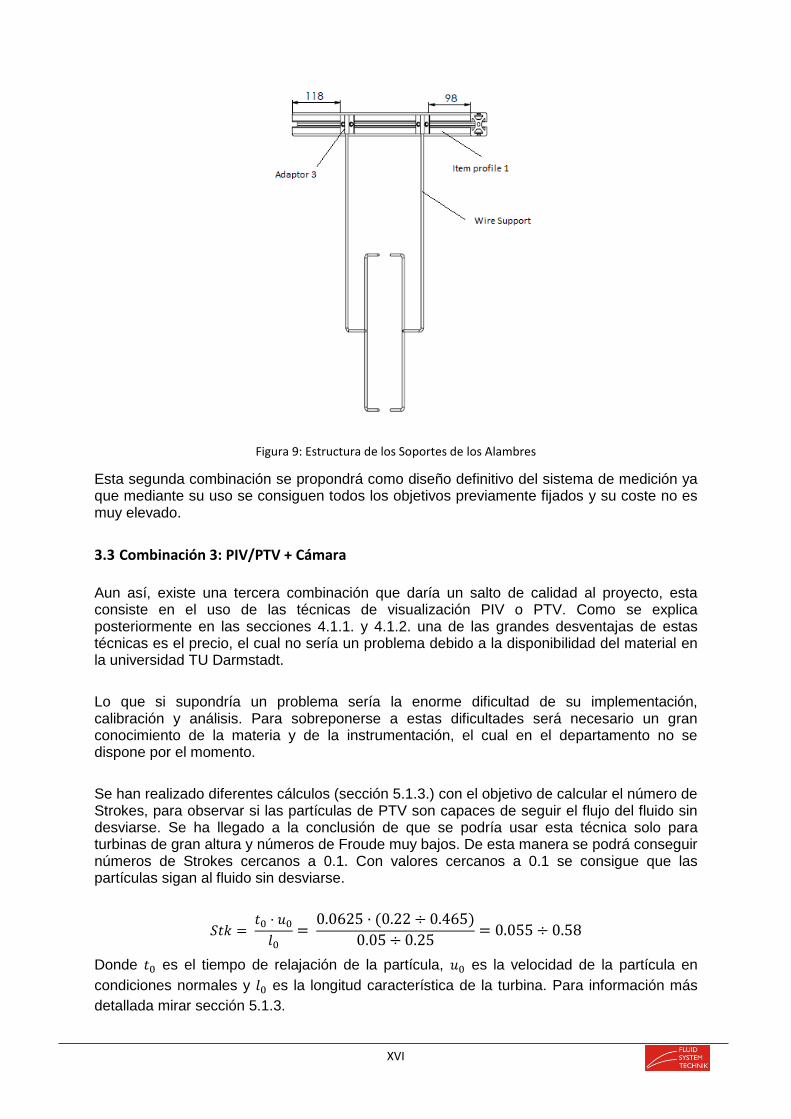
En la Figura 9 se puede observar el conjunto de los alambres de platino usados para la
generación de burbujas de hidrógeno. Este conjunto está detalladamente explicado en la
sección 5.2.
XVI
Figura 9: Estructura de los Soportes de los Alambres
Esta segunda combinación se propondrá como diseño definitivo del sistema de medición ya que mediante su uso se consiguen todos los objetivos previamente fijados y su coste no es muy elevado.
3.3 Combinación 3: PIV/PTV + Cámara
Aun así, existe una tercera combinación que daría un salto de calidad al proyecto, esta consiste en el uso de las técnicas de visualización PIV o PTV. Como se explica posteriormente en las secciones 4.1.1. y 4.1.2. una de las grandes desventajas de estas técnicas es el precio, el cual no sería un problema debido a la disponibilidad del material en la universidad TU Darmstadt.
Lo que si supondría un problema sería la enorme dificultad de su implementación, calibración y análisis. Para sobreponerse a estas dificultades será necesario un gran conocimiento de la materia y de la instrumentación, el cual en el departamento no se dispone por el momento.
Se han realizado diferentes cálculos (sección 5.1.3.) con el objetivo de calcular el número de Strokes, para observar si las partículas de PTV son capaces de seguir el flujo del fluido sin desviarse. Se ha llegado a la conclusión de que se podría usar esta técnica solo para turbinas de gran altura y números de Froude muy bajos. De esta manera se podrá conseguir números de Strokes cercanos a 0.1. Con valores cercanos a 0.1 se consigue que las partículas sigan al fluido sin desviarse.
𝑆𝑡𝑘 = 𝑡0 · 𝑢0
𝑙0=
0.0625 · (0.22 ÷ 0.465)
0.05 ÷ 0.25= 0.055 ÷ 0.58
Donde 𝑡0 es el tiempo de relajación de la partícula, 𝑢0 es la velocidad de la partícula en
condiciones normales y 𝑙0 es la longitud característica de la turbina. Para información más
detallada mirar sección 5.1.3.

XVII
4 Diseño de la Estructura de la Turbina
El principal problema de la estructura de la turbina anterior a este trabajo era el arduo
trabajo que se necesita para operar con el plato perforado, esto significa que, a la hora de
cambiar la posición de la turbina, cambiar su resistencia o su tamaño es necesario la
utilización de tornillos, implicando unos mayores tiempos de preparación de los
experimentos al cambiar alguna característica de la turbina.
Por tanto, el objetivo será encontrar un sistema que sea más automático con el objetivo de
acelerar el proceso de recolección de datos cuando la turbina esté posicionada en diferentes
posiciones y con diferentes características.
Se propone una estructura compuesta por un husillo de bolas, un motor de paso a paso y una caja de cambios. Mediante el uso de este sistema se consigue fácilmente controlar el cambio de posición del plato perforado mediante código en Labview y usando un controlador que estará posicionado fuera del canal de pruebas. Programar en Labview está más allá de este trabajo y será responsabilidad de la persona encargada de llevar a cabo el experimento.
Este mecanismo permite recolectar datos no solo en una posición, sino en diferentes posiciones del plato perforado en menor tiempo que la estructura actual la cual a diferencia de un sistema automático se basa en atornillar y desatornillas el plato perforado al soporte de la turbina. (Sección 2.3.)
Con este sistema propuesto solo es necesario atornillar a la hora de cambiar el tamaño del plato perforado, por lo que el procedimiento de la recolecta de datos debería consistir en tomar todos los datos acordes a un tamaño de plato perforado determinado en diferentes posiciones y con diferentes resistencias y después cambiar el tamaño del plato, y así sucesivamente. Con la anterior estructura, era necesario atornillar siempre que se quiera cambiar la posición, la resistencia o el tamaño del plato perforado.
Otra ventaja de este mecanismo es el hecho de poder posicionar el plato perforado por encima del canal de pruebas de manera que al cambiar el tamaño de los platos perforados sea más cómodo y no haga falta atornillar dentro del canal de pruebas como era necesario anteriormente. Para ello es necesario que el soporte de la turbina (ver sección 5.1.2.1. y sección 10) sea más largo que el actual.
Los planos de las piezas del adaptador L y el adaptador 1 se pueden encontrar en la sección
10. El resto de piezas deben de ser compradas a los proveedores indicados en la sección
6.1. Además, en dicha sección están indicadas las funcionalidades de cada pieza.
Posicionando el husillo de bolas lateralmente al flujo, se evita que la estructura balancee, ya
que la superficie normal al flujo es menor que la superficie transversal, lo cual da más rigidez
a la estructura. Aunque está opción es eficiente, posee una desventaja y esta es la aparición
de un momento indeseado. Este momento no es muy grande ya que se ha diseñado de
manera que la distancia entre el soporte de la turbina y el husillo de bolas sea menor de 5
cm.

XVIII
Figura 10: Estructura de la Turbina Lateral
Existe otra opción, la cual consiste en que el husillo de bolas sea frontal al flujo, esta
finalmente no ha sido considerada ya que la estructura podría balancear modificando la
posición de la turbina constantemente, véase la sección 6.1. Figura 50.
Aunque el mecanismo seleccionado ha sido la opción lateral al flujo, ambos mecanismos,
lateral y frontal, poseen prácticamente las mismas piezas, por lo que podría ser una buena
idea experimentar con ambos mecanismos.

XIX
5 Elección de Resistencias de la Turbina sobre el Flujo
Para la elección de resistencias el objetivo es intentar disipar la mínima energía posible, esto
significa buscar un coeficiente de resistencia lo más bajo posible. En la siguiente ecuación
se relaciona el coeficiente de resistencia con el coeficiente de sección transversal. (Idel’chik.
Handbook of Hydraulic Resistance [Coefficients of Local Resistance and of Friction]. , 1966.)
𝜉 = (0.707√1 − Φ + 1 − Φ)2 ·1
Φ2
Φ = 𝐴𝑜𝑝𝑒𝑛
𝐴𝑐𝑙𝑜𝑠𝑒
Esto significa que, a mayor coeficiente de sección transversal, menor será el coeficiente de
resistencia. Por lo tanto, será más conveniente usar platos perforados con agujeros
cuadrados que con agujeros redondos, ya que un plato perforado con agujeros redondos
posee una mayor área cerrada y consecuentemente un menor coeficiente de sección
transversal.
Por ello finalmente, se fabricarán tres resistencias con agujeros cuadrados de lado 5, 8 y 10
mm y con una distancia entre centros de 8, 12 y 15 mm respectivamente.
Se fabricarán cinco diferentes tamaños de platos perforados, la anchura será la misma que
la del canal de pruebas para conseguir una obstrucción completa (200 mm) pero la altura
tomará los valores de 50 mm, 100 mm, 200 mm, 250mm y 400mm.
Los materiales y su coste están detalladamente explicados en la sección 6.2., la siguiente
figura refleja la forma de las resistencias con agujeros cuadrados.
Figura 11: Resistencia de la Turbina

XX

XXI
6 Conclusiones y Trabajos Futuros
En vista de todo lo mencionado anteriormente, es conveniente realizar varias conclusiones acerca del
presente TFG. El sistema de medición se puede dividir en la medición de la velocidad y la medición
del nivel de altimetría del fluido en el canal.
La velocidad será medida mediante una técnica de Visualización del Flujo, más concretamente con el
método de generación de burbujas de hidrógeno, la consola eléctrica usada para generar las
burbujas por electrólisis es la mostrada en la Figura 5, el alambre generador de burbujas será de
platino y su soporte de latón, la longitud del alambre será de 250 mm con el objetivo de cubrir toda
la altura del canal y la iluminación del área de interés se realizará mediante un sistema de LEDs. Con
este sistema será posible medir la distribución de velocidades, la línea media y la anchura del tubo de
corriente generado por la turbina entre los puntos (-) y (2). Se usará un tubo de Pitot para medir el
perfil de velocidades en la zona entre los puntos (1) y (+).
La medición del nivel del agua se realizará mediante la misma cámara de alta resolución usada en el
método de las burbujas de hidrógeno. En la TU Darmstadt se dispone de la cámara Sensicam.qe.
Realizando un número considerable de fotos e interpolando no será de gran dificultad medir la
altimetría del nivel del fluido. Se considera innecesario usar otras técnicas de mayor dificultad como
láseres o métodos ultrasónicos.
La estructura de la turbina diseñada en este trabajo consiste en un husillo de bolas, un motor paso a
paso, una caja de cambios y un controlador. El movimiento vertical de este sistema será codificado
mediante Labview. Este mecanismo permite medir los parámetros requeridos en diferentes alturas y
con diferentes resistencias sin el uso de tornillos. El único momento donde será necesario el uso de
tornillos será a la hora de cambiar el tamaño del plato perforado.
Con este mecanismo se gana rapidez a la hora de recolectar datos y comodidad a la hora de manejar
la estructura de la turbina.
Dicha estructura tendrá el husillo de bolas posicionado lateralmente al flujo, de manera que se
pueda evitar el balanceo de la estructura. La distancia entre el husillo de bolas y el soporte de la
turbina será mínima con objeto de evitar un momento indeseable. Todas las piezas de estos
conjuntos están detalladas en la sección 10.
Aunque la técnica de la generación de burbujas de hidrógeno es eficiente, si se quiere dar un salto de
calidad en el proyecto, es recomendable usar técnicas como PIV o PTV, las cuales son mucho más
precisas. Por tanto, el siguiente paso podría ser la implementación de una de estas técnicas. Si este
no es el camino a seguir y se decide usar la técnica de la generación de burbujas de hidrógeno, sería
conveniente iluminar el área de interés con láminas de láser en vez de con LEDs.

XXII
La persona responsable en la realización del experimento deberá calibrar los aditivos y la señal de
entrada al multivibrador TTL mediante los parámetros 𝑅1 y 𝐶1 explicados en la sección 5.1.2.2.
Además es recomendable probar las dos estructuras propuestas en el presente trabajo: la opción
lateral y frontal, ya que poseen piezas bastante similares.

XXIII
Tabla de Figuras Del Resumen en Español
Figura 1: Simulación Experimental del Flujo ......................................................... VI
Figura 2: Canal de Pruebas 3D ......................................................................................... VII
Figura 3:Canal de Pruebas 2D ............................................................................................ VII
Figura 4: Visualización del Flujo mediante Láminas ....................................... XII
Figura 5: Circuito Electrónico para la Generación de Burbujas de
Hidrógeno .................................................................................................................... XIII
Figura 6: Visualización del Flujo ............................................................................... XIV
Figura 7: Soporte para Sonda Vertical ..................................................................... XIV
Figura 8: Estructura del Tubo de Pitot .................................................................... XV
Figura 9: Estructura de los Soportes de los Alambres ................................. XVI
Figura 10: Estructura de la Turbina Lateral ..................................................... XVIII
Figura 11: Resistencia de la Turbina ........................................................................ XIX


S286
Conception and Design of a
Velocity and Water Level
Profile Measurement
System for a Channel Test
Rig Konzeption und Auslegung einer Messeinrichtung zur Messung von
Geschwindigkeits- und Pegelprofilen an einem Gerinnenprüfstand
Álvaro Quiles García, Supervisor: Christian Schmitz, M.Sc.
Bachelor Thesis, Darmstadt, 12.07.2017
Prof. Dr.-Ing. Peter Pez.


Erklärungen
Hiermit versichere ich, die vorliegende Diplomarbeit ohne Hilfe Dritter nur mit den
angegebenen Quellen und Hilfsmitteln angefertigt zu haben. Alle Stellen, die den Quellen
entnommen wurden, sind als solche kenntlich gemacht worden. Diese Arbeit hat in
gleicher oder ähnlicher Form noch keiner Prüfungsbehörde vorgelegen.
(Ort,Datum) (Unterschrift)


Acknowledgments
I would like to express my sincere thanks to Prof. Dr.-Ing. Peter Pelz, Principal of the Department, for
providing me with all the necessary facilities for the research.
I place on record, my sincere thanks to Christian Schmitz, who has been the supervisor of this
bachelor thesis. I am extremely thankful and indebted to him for sharing expertise and valuable
guidance, also for his continuous encouragement.
I take this opportunity to express gratitude to all of the FST Department members for their help and
support. I also thank my family for the unceasing encouragement, support and attention, they made
possible that I had the opportunity to do my bachelor thesis in TU Darmstadt.
Finally I want to thank the support of my Erasmus family from Darmstadt, which have support me in
the good and the bad times throughout this year.


I
Table of Contents
1 INTRODUCTION .............................................................................................................. 7
2 MOTIVATION ................................................................................................................. 9
2.1 Experiment Technical Fundamentals ....................................................................................... 9
2.1.1 Basic Explanation of the Flow Simulation ................................................................................... 9
2.1.2 Conservation of Mass ............................................................................................................... 10
2.1.3 Conservation of Momentum and Energy. ................................................................................ 11
2.1.4 Dimensionless Numbers ........................................................................................................... 13
2.1.4.1 Number of Reynolds .......................................................................................................... 13
2.1.4.2 Froude Number .................................................................................................................. 14
2.1.4.3 Stokes Number ................................................................................................................... 16
2.1.5 Specific Energy and Critical Flow .............................................................................................. 18
2.2 Test rig ................................................................................................................................. 19
2.3 Current Problems.................................................................................................................. 23
2.3.1 Measurement system ............................................................................................................... 23
2.3.2 Turbine System ......................................................................................................................... 24
3 OBJECTIVES .................................................................................................................. 27
4 RESEARCH .................................................................................................................... 31
4.1 Velocity Measurements ........................................................................................................ 31
4.1.1 Particle Image Velocimetry (PIV) .............................................................................................. 32
4.1.2 Particle Tracking Velocimetry (PTV) ......................................................................................... 33
4.1.3 Pitot Tube ................................................................................................................................. 34
4.1.4 Multi-hole Probe ....................................................................................................................... 35
4.1.5 Hot Wire Probe ......................................................................................................................... 36
4.1.6 Laser Doppler Anemometry...................................................................................................... 38
4.1.7 Molecular Tagging Velocimetry ................................................................................................ 40
4.1.8 Flow Visualization ..................................................................................................................... 40
4.2 Water Level Measurements .................................................................................................. 46
4.2.1 Camera ...................................................................................................................................... 46
4.2.2 Laser Distance Sensor ............................................................................................................... 47
4.2.3 Conductive Level Altimetry ....................................................................................................... 48
4.2.4 Capacitive Level Altimetry ........................................................................................................ 49
4.2.5 Direct Measurement ................................................................................................................. 50
4.2.6 Ultrasonic Level Transmitter ..................................................................................................... 50

II
4.2.7 Radar Level Altimetry ............................................................................................................... 51
4.2.8 Magnetostrictive Level Transmitter ......................................................................................... 52
5 MEASUREMENT CONCEPT ............................................................................................ 53
5.1 Election of the Concept ......................................................................................................... 53
5.1.1 Pitot Tube + Conductive Level Altimetry .................................................................................. 53
5.1.2 Flow Visualization + Pitot tube + Camera ................................................................................. 53
5.1.2.1 Polyethylene Foils Concept ................................................................................................ 53
5.1.2.2 Hydrogen Bubbles Generation Concept ............................................................................ 55
5.1.3 PIV/PTV + Camera Concept....................................................................................................... 62
5.2 Design of the Construction of the Measurement System. ....................................................... 63
6 TURBINE CONCEPT ....................................................................................................... 65
6.1 Election of the Turbine Concept ............................................................................................ 65
6.2 Election Turbine Resistances ................................................................................................. 69
7 SUMMARY AND OUTLOOKS ......................................................................................... 73
7.1 Summary .............................................................................................................................. 73
7.2 Outlooks ............................................................................................................................... 74
8 REFERENCES ................................................................................................................. 75
9 APPENDIX A ................................................................................................................ 77
9.1 List of Figures ....................................................................................................................... 77
9.2 List of Tables ......................................................................................................................... 78
9.3 Economic Budget .................................................................................................................. 79
9.4 Planning – Diagram of Gantt ................................................................................................. 81
10 APPENDIX B – TECHNICAL DRAWINGS ........................................................................ 83

III
List of Symbols
Base System
The first column in the following list shows the symbols used in the text for the occurring physical
and mathematical quantities. The meaning of the symbol is described in the second column. The
dimension formula of each physical quantity is given in the third column as the power product of the
basis variables length (L), mass (M), time (T), temperature (ϴ), quantity of substance (N), current (I)
and light intensity (J)
Symbol Description Dimension
𝑢 Velocity of the flow 𝐿 𝑇−1
ℎ Water level 𝐿
𝐴𝑡 Streamtube wide 𝐿
𝑍𝑡 Streamtube medium line 𝐿
�̇� Mass flow 𝑀 𝑇−1
𝜌 Density 𝑀 𝐿−3
𝑉 Volume 𝐿3
𝐴 Area 𝐿2
𝑡 Time 𝑇
𝑒 Internal energy 𝐿2 𝑇−2
𝑘 Kinetic energy 𝐿2 𝑇−2
𝑞 Heat flux 𝑇−3
𝑅ℎ Hydraulic raidus 𝐿
𝑝𝑤 Perimeter wetted 𝐿
𝑅𝑒 Reynolds number 1
𝜈 Kinetic viscosity 𝐿2 𝑇−2
𝜇 Dinamic viscosity 𝑀 𝑇−1 𝐿−1
𝑏 Width of the channel 𝐿
𝑎 Height of the channel 𝐿
𝑔 Gravity 𝐿 𝑇−2
𝐷ℎ Hydraulic Diameter 𝐿

IV
𝐹𝑟 Froude number 1
𝛿 Distance between turbine and
channel
𝐿
𝑆𝑡𝑘 Stokes number 1
𝑙 Characteristic dimension of
turbine
𝐿
𝑑 Diameter 𝐿
𝐻 Hydraulic head 𝐿
𝑄 Volume Flow 𝐿3 𝑇−1
𝑝𝑠 Static pressure 𝑀 𝐿 𝑇−2
𝜎 Dimensionless turbine width
position
1
휁 Dimensionless turbine height
position
1
𝛼 Dimensionless streamtube
width
1
𝜉 Dimensionless streamtube
height
1
𝑅 Gas constant 𝐿2 𝑀 𝑇−2 𝛩−1 𝑁−1
𝑠 Wall depth 𝐿
𝑈 Voltage 𝑀 𝐿2 𝐼−1 𝑇−3
𝑅 Resistance 𝑀 𝐿2 𝑇−2 𝐼−2
휀 Permittivity 𝑀−1 𝐿−3 𝑇4 𝐼2
𝐶 Capacitance 𝑀−1 𝐿−2 𝑇4 𝐼2
𝑓 ̅ Cross-section coefficient 1
𝜉 Resistance coefficient 1

V
Subscripts Definition
1 Entrance of the channel
+ Just before the perforated plate
- Just after the perforated plate
2 Beginning of the Mixture Zone
3 Homogeneous fluid
2o Outside the streamtube
2i Inside the streamtube
CV Control Volume
0 Far from the perforated plate
P Tracer particle
C Critic
Abbreviation Definition
TU Technische Universität
HDP High Density Polyethylene
LDP Low Density Polyethylene
DC Direct Current
TTL Transistor-Transistor Logic

VI

7
1 Introduction
After decades using fossil fuels to generate electricity, the principal organisations, which defend the
environment, are starting to encourage governments to use green energy from renewable energies.
In the following picture it can be observed the final consumption of the Renewable Energies in the
world at the year of 2015.
Figure 1: Final Energy Consumption 2015 [1]
The present thesis is going to be focused on the hydropower energy, which is only the 3.6% of the
total energy consumption of the world. More concretely it will be focused on Tidal turbines. Talking
about Tidal energy, it is worthy to mention that experts assure that the future of this energy looks
really consistent due to the more efficient underwater turbines which will appear in the following
years. [2]
The main problem nowadays is the high cost involved in the whole process, because of that during
these days it is difficult to compete against the traditional electric companies, which offer a really
competitive price. The main objective in the following years should be to come down the high
construction costs due to a better efficiency of the materials. [3]
In [4], it is designed a model to calculate the performance factor 𝐶𝑝 for a hydroelectric power station
in a rectangular channel with complete obstruction in width and height. There have been several
studies about it, for instance [5], where the developed method is extensively extended in such a way
that the turbine has a complete obstruction in height but at the same time is bypassed horizontally
by a bypass.

8
In contrast to conventional power plants, tidal turbines are placed freely in the flow and do not have
a complete obstruction. The present thesis studies a complete obstruction in width but not in height,
leading to a vertical by-pass flow.
The influence of the free surface on the turbine is the main problem at the time of designing the
measurement system, due to the cascade produced by the presence of the turbine, which generates
a difference of static energy. The analytical model, which is the basis of this thesis, was done by using
energy conservation, continuity equation and the principle of linear momentum [6].
The construction of the test rig was designed in [7] and improved in [8]. The main objective of the
present thesis is to improve the measurement system designed by [9] and [8]. The concept should be
able to measure the velocity of the flow, the medium line and the width of the streamtube and
finally the water level altimetry.
Another important part of the thesis will consist in designing a system which can improve the
management of the turbine changes, that means a more automatic system instead of a manual
system that is principally based in screwing when is necessary to change any position or
characteristic of the turbine.
The present thesis will therefore focus on the research, design and implementation of a
measurement system which fulfils the requirements and the design of a more manageable turbine
structure.

9
2 Motivation
2.1 Experiment Technical Fundamentals
2.1.1 Basic Explanation of the Flow Simulation
This experiment consists in the modulation of the flow from a real Tidal Turbine, where a perforated
plate will be use instead of a normal turbine. The perforated plate will have a complete width but a
variable height, which will produce a vertical by-pass flow.[6]
It has been chosen this kind of “turbine” due to different reasons:
Although the perforated plate dissipates heat instead of mechanic energy, which will be later
convert in electricity, this prototype is used due to the fact that it does not matter which kind
of energy it dissipates, the final results will be exactly the same.
It represents a By-pass flow, which is characteristic of a tidal turbine in comparison to
conventional hydro-power stations where there is not by-pass flow.
Figure 2 represents the flow model of the experiment, with a vertical by-pass flow generated due to
the perforated plate previously commented.
Figure 2 Flow Simulation of the Experiment [10].
10
As it can be observed in the Figure 2, there are 5 important points along the channel test rig. (1),(+),(-
),(2) and (3). The area of interest of this thesis consists of the interval between points (+) and (2). This
area is what it is called: “Area of interest” only in this thesis.
The Area of interest includes a cascade produced by the presence of the perforated plate, this
cascade will lead to a difference of static energy due to the difference of heights between the points
(+) and (-). This difference of static energy is going to be a relevantt part of the dissipated energy,
which the perforated plate produces, so it is of great importance.
Another relevant consequence of using a by-pass flow turbine is the difference of velocity between
the water which passes through the turbine and the one from the by-pass flow ( 𝑢20 > 𝑢2𝑖 ).
This fact is interesting because there will be a conservation of the volume flow until the mixing zone
as it can be seen in Figure 2.
2.1.2 Conservation of Mass
The principle of mass conservation assures that for a closed system, the mass of the entire system
should remain constant without any variation along the time. There is a popular statement which
says that “mass can neither be created nor destroyed”. This statement means that if the mass added
is the same as the mass removed in a control volume the variation of mass flow in the control
volume is cero. [11] 𝑑𝑚𝑐𝑣
𝑑𝑡= 0 (Steady-flow process).
�̇�𝑖𝑛 − �̇�𝑜𝑢𝑡 = 𝑑�̇�𝑐𝑣
𝑑𝑡= 0 (Eq. 1)
If a mass balance is done to a steady-flow process like the one it is used in this thesis the mass that
flows in or out of the channel must be the same.
Usually this principle is represented as in the Eq.2 but in this case we only have one possible entrance
and one possible exit so it is possible to eliminate the summations. [11]
∑ �̇�𝑖𝑛 = ∑�̇�𝑜𝑢𝑡 (Eq. 2)
As it is known from the Reynold’s transport theorem [11] the mass flow in the control volume is
constant.
𝑑𝑚
𝑑𝑡|𝐶𝑀
=𝑑
𝑑𝑡∫ 𝜌𝑑𝑉
𝐶𝑉+ ∫ 𝜌(�⃗� 𝑟𝑒𝑙 · �̂�)𝑑𝐴
𝐶𝑆 (Eq. 3)
It is possible to simplify this equation: [11]
As it was said before: 𝑑𝑚
𝑑𝑡|𝐶𝑀
= 0

11
It is considered that the fluid is incompressible, in the case of this experiment the fluid will be
water, and hence the density of the water between different sections is constant. 𝑑
𝑑𝑡∫ 𝜌𝑑𝑉
𝐶𝑉= 0
So finally the principle of mass conservation leads to the following formula with the conditions of the
experiment 𝜌 is constant due to the incompressibility of the liquid. [11]
0 = ∫ 𝜌(�⃗� 𝑟𝑒𝑙 · �̂�𝑑𝐴)
𝐶𝑆= 𝜌 · 𝑢𝑜𝑢𝑡 · 𝐴𝑜𝑢𝑡 − 𝜌 · 𝑢𝑖𝑛 · 𝐴𝑖𝑛 = ∑𝑄𝑖𝑛 − ∑𝑄𝑜𝑢𝑡 (Eq. 4)
In the Figure 3 it can be observed a Control Volume in a steady-flow with a variant cross section. Eq.
5 and Eq. 6 are the formulas applied from Eq.4 to this case, which is the same as our experiment.
Figure 3: Control Volume with variant cross-section [7]
∑𝑄1 = ∑𝑄2 (Eq. 5)
𝑢1 · 𝐴1 = 𝑢2 · 𝐴2 (Eq. 6)
It is important to notice that there is continuity in the equations and that the velocities are
proportional to each other by a relationship between the cross sections of the entrance and exit of
the control volume.
This mass conservation principle will lead to a volume flow conservation and it will be important in
the Measurement Concept election as it will be explain in the following sections.
2.1.3 Conservation of Momentum and Energy.
These two principles are not that relevant, as the principle of mass conservation, for this thesis, even
so they should be mentioned because they were very important for the modelling process. By using
these principles it is possible to get some equations of interest for the modelling.

12
Figure 4: Volume and Surfaces Forces. [7]
The Figure 4 shows the depiction of the two kinds of forces that appear in the formula of the
momentum conservation, surface forces and volumetric ones.
The principle of energy conservation states that within some domain, the energy is neither created
nor destroyed but it remains constant. That means that energy can be transformed in other kind of
energies but the energy of the whole system must be constant. [12]
𝐷
𝐷𝑡∭ [
𝑢𝑖𝑢𝑖
2+ 𝑒] 𝜌𝑑𝑉 = ∭ 𝑢𝑖𝑘𝑖𝜌𝑑𝑉 + ∬ 𝑢𝑖𝑡𝑖𝑑𝑆 − ∬ 𝑞𝑖𝑛𝑖𝑑𝑆
𝑆
𝑆
𝑉
𝑉(𝑡) (Eq. 7)
The momentum can be defined as the mass of an object multiplied by its velocity. The principle of
momentum conservation states that the momentum is neither created nor destroyed. It remains
constant within a domain. It can only be changed by the action of some forces. The main complexity
of this principle in comparison with the mass and energy conservation resides in the fact that the
momentum is a vector quantity. This means that the conservation must be in the three directions at
the same time. [12]
After using the Reynold’s transport theorem it is obtained: [13]
∭𝜕(𝜌·�⃗⃗� )
𝜕𝑡𝑑𝑉 + ∬ 𝜌 · �⃗� (�⃗� · �⃗� )𝑑𝑆 = ∭ 𝜌�⃗� 𝑑𝑉 + ∬ 𝑡 𝑑𝑆
𝑆
𝑉
𝑆
𝑉 (Eq. 8)

13
2.1.4 Dimensionless Numbers
2.1.4.1 Number of Reynolds
Before defining the Reynolds number it is necessary to take into account that the experiment is done
in an open channel test rig. Consequently, there is a characteristic value called the hydraulic radius:
[13]
𝑅ℎ =𝐴
𝑝𝑤 (Eq. 9)
𝐴 means the Area and 𝑝𝑤 means the wetted perimeter.
In our channel the perimeter is 1.000 mm and the cross-section is 80.000 mm2. Resulting:
𝑅ℎ = 80 mm
The number of Reynolds can be defined as a relationship between the inertial forces and the viscous
forces. This dimensionless number is defined in the following equation [13]
𝑅𝑒 =𝜌·𝑈·𝑅ℎ
𝜇=
𝑈·𝑅ℎ
𝜈 (Eq. 10)
An important issue about this number is that it can define the behaviour of the flow as laminar flow
or turbulent flow. [13]
A laminar flow appears in an open channel when the Reynolds number is low ( 𝑅𝑒 < 500 ), this
means that the viscous forces are dominant in comparison with the inertial forces. This kind of flow is
characterized by a constant and smooth fluid motion. Normally this behaviour happens when the
velocities are really low.
Talking about the turbulent flow, which appears in a typical open channel test rig, it is necessary to
have a Reynolds number higher than in the laminar flow (𝑅𝑒 > 2000). A turbulent flow is
characterised by the domination of inertial forces in comparison with viscous forces in addition to
the many vortices and flow instabilities in the fluid.
It is important bearing in mind that there is a transition state when the Reynolds number is between
the laminar flow and the turbulent flow.
A more accurate formula for open channel test rigs is the following equation: [10]
𝑅𝑒 =4·𝑢𝑜·ℎ0
(1+2ℎ0𝑏
)𝜈 (Eq. 11)
By using this formula depending on the volume flow which is introduced to the channel, it is obtained
a range of the Reynolds number between 7 · 104 ÷ 3 · 105. In section 2.2 is detailed this calculation
This means that the flow of the experiment is going to have always a turbulent behaviour.

14
2.1.4.2 Froude Number
The Froude number can be defined as the relationship between the inertial forces and the gravity
forces. It is a dimensionless number which defines whether the flow is critical or uncritical. [13]
In open channels there is a characteristic value:
𝐷𝐻 =4·𝑎·𝑏
2𝑎+𝑏 (Eq. 12)
The Froude number is defined as the following equation: [13]
𝐹𝑟 =𝑢
𝑔√𝐷ℎ (Eq. 13)
As it has been mentioned before, the Froude number can delimitate when the flow state is critical:
[13]
𝐹𝑟 < 1: The flow is subcritical, which means a tranquil and slow fluid, where the gravity
forces dominate over the inertial forces.
𝐹𝑟 = 1: The flow is critical, it will be more detailed in section 2.1.5
𝐹𝑟 > 1: The flow is supercritical, which means a fast rapid fluid, inertial forces dominate in
comparison with gravity forces.
In our experiment the Froude number at the entrance of the channel is between 0-0.3 m/s, at the
end of the channel is between 0-0.5 m/s, but just after the perforated plate, in the cascade the flow
is supercritical with a maximal Froude number around 1.4.
So the flow has a subcritical behaviour in the whole channel except for the area close to the
perforated plate where is produced the hydraulic jump.
Figure 5 shows a graphic implicating the Reynolds number and the Froude number and the different
possible states of the flow in an open channel test rig.
15
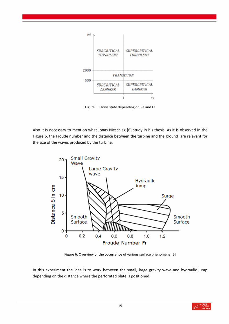
Figure 5: Flows state depending on Re and Fr
Also it is necessary to mention what Jonas Nieschlag [6] study in his thesis. As it is observed in the
Figure 6, the Froude number and the distance between the turbine and the ground are relevant for
the size of the waves produced by the turbine.
Figure 6: Overview of the occurrence of various surface phenomena [6]
In this experiment the idea is to work between the small, large gravity wave and hydraulic jump
depending on the distance where the perforated plate is positioned.

16
The main aspect of Figure 6 is that the picture can show the relevance of the turbine’s position in the
test rig, because the results differ a lot in different positions.
Figure 7, Figure 8 and Figure 9 show three different types of waves explained in Figure 6: Small
gravity waves, large gravity waves and hydraulic jump.
Figure 7: Small Gravity Wave [6]
Figure 8: Large Gravity Wave [6]
Figure 9: Hydraulic Jump [6]
2.1.4.3 Stokes Number
The Stokes dimensionless number (Stk) is defined as the ratio between the characteristic time of a
particle and the characteristic time of the flow through an obstacle. [14]

17
𝑆𝑡𝑘 =𝑡0·𝑢0
𝑙0 (Eq. 14)
The parameter 𝑡0 is called as the relaxation time or stopping time of the particle, conventionally it is
computed applying the Stokes (linear) drag law to a particle initially moving with the free stream
velocity. The parameter 𝑢0 is the fluid velocity of the flow in normal conditions and the parameter 𝑙0
is the characteristic dimension of the obstacle, in our case it would be the height of the perforated
plate. [14]
If the particles Reynolds is lower than 1, it means that the particles follow a stokes flow, and the
relaxation time parameter can be defined as follows: [14]
𝑡0 =𝜌𝑝·𝑑𝑝
2
𝜇𝐻20 (Eq. 15)
In case of using optical methods as PIV or PTV with particle tracers it is necessary to have a low
stokes number, a low stokes number 𝑆𝑡𝑘 ≪ 1 means that the particles will follow the fluid
streamlines, whereas if the stokes number of a particle is too large, it continues along its initial
trajectory. [14]
The idea is to get stokes number lower than 1 and if it is possible, lower than 0.1, which leads to an
error between the streamlines of the flow and the particles lower than 1%.
In the following picture, it is observed three cases depending on the strokes number between a solid
particle and a liquid flow like water. In the first case the particle and the flow have the same stream
line, whereas in the third case they have completely different streamlines as it was explained before.
Figure 10: Stokes Number Behaviour of the Flow

18
2.1.5 Specific Energy and Critical Flow
The specific energy of the flow in the open channel is composed by a part of kinetic energy (velocity)
in addition to a part of potential energy (depth). Usually in an open channel it is necessary to
determinate the energy of the fluid in a particular section of the test rig. [11]
𝐻 = ℎ +𝑢2
2𝑔 (Eq. 16)
In our case the energy of the fluid at the entrance of the channel is 𝐻1 = 250 mm [15].
Where ℎ means depth and �̅� the average velocity [13], note that the velocity depends on the volume
flow and the cross-section.
𝑢 =𝑄
𝑏·ℎ (Eq. 17)
This dependence is important because the specific energy will depend on the depth in both addends.
Figure 11 shows a graph between the specific energy and the depth of the fluid. [13].
This specific energy will be of interest when designing the dimensions of some pieces which are in
touch with the water.
Figure 11: Specific energy with Fluid depth
There should be done some comments about Figure 11: [9]

19
The line of 45º defines 𝐻 = ℎ
For any point on the curve (H,h) the horizontal distance between the h-axis and 45º-line is
the potential energy, whereas the horizontal distance between the 45º-line and the
mentioned point of the curve is the kinetic energy
It is important to talk about the point in the curve, where the specific energy is minim, this
occurs in the moment of critical flow 𝐹𝑟 = 1.
At the critical state it can be found the critical depth ℎ𝑐
The critical depth defines if the fluids flow is supercritical or subcritical. In the case that ℎ < ℎ𝑐 the
flow behaves supercritical, whereas if ℎ > ℎ𝑐 the flow behaves subcritical.
As it is observed in Figure11, in the curve (H-h) there are two points with the same specific energy
but the difference between them relies on the fact that the one above the critical depth produces a
subcritical flow, while the point below the critical depth produces a supercritical flow. [13].
2.2 Test rig
The test rig used in this experiment is the one shown in the Figure 12 and Figure 13, it can be defined
as a closed loop because the channel is provided by the same water all the time. An important
element of the test rig is the electric water pump, which provides water to the channel. This water
comes from a water tank, which is below the outlet of the channel.
Figure 12: Test rig 3D [10].

20
Figure 13: Test rig 2D [10]
There are some relevant aspects which are important to comment briefly:
The inlet part of the channel is made of stainless steel and it has a round-shaped bottom so that
there can be a progressively develop of the boundary layer and also a better velocity profile which is
going to arrive later to the turbine. [7]
Also in the inlet part, as it can be observed in Figure 13 there is a baffle plate and a homogenizer
which provides the channel a balance flow, moreover it affects in a good way to the velocity profile
by which will be more realistic due to the importance of having a homogenized flow. [7]
The volume flow rate through the channel is controlled by changing the position a movable wall in
the outlet section. The volume flow (𝑄) in addition to the Froude number (section 2.1.4.2.) and some
other parameters, such as the position (𝑧𝑡 = 휁 · 𝐻1) (Figure 6) and width (𝐴𝑡 = ℎ1 · 𝑏 · 𝜎) of the
turbine are relevant when controlling the flow of the experiment.
Another relevant aspect of the test rig is the material of the channel. This material is acrylic-glass,
this material has been chosen due to its transparency. The usage of this material is interesting
because it allows working with optical techniques of measurement such as PIV, PTV or even Flow
Visualization; this information will be relevant for the election of the measurement system.
It is also important to talk about the measurement section of the channel; D. Hernández worked on
the construction of the test rig in his Bachelor Thesis [7], the maximum height was calculated in this
work by relating the height with the Froude number in order to decide which channels height would
be sufficient.
By using Eq.13 and Eq.17 we arrive to Eq.18 and Eq. 19.

21
ℎ = (�̇�2
𝐹𝑟2𝑔𝑏2)1
3⁄ (Eq. 18)
𝑢 = ( 𝐹𝑟√𝑔𝑄
𝑏 )2/3 (Eq. 19)
By considering a Froude number of 0.5 and the volume flow 82 m3 /h. The result of the maximal
height is h= 0.174 m, but as one of the most important aspects of construction is the flexibility it was
decided to make it over dimensional with a maximum height of 40 cm. [7]
Now it is possible to calculate the velocity for a Froude number of 0.1 by using Eq. 17 𝑢 =�̇�
𝑏·ℎ=
0.22 m/𝑠
A more interesting value is the velocity in the point of supercritical flow (Fr=1.4) just after the
cascade. In this case the velocity will be the maximum one 𝑢𝑚𝑎𝑥 = 1.29 m/𝑠 with ℎ(𝐹𝑟 =
1.4) = 0.087 m.
By using this data and Eq.11 the maximal Reynolds in the area of interest just after the turbine is
𝑅𝑒𝑚𝑎𝑥 = 2,4 · 105, which is clearly a turbulent behaviour of the flow. (See section 2.1.4.) 𝑅𝑒(𝐹𝑟 =
0.1 ÷ 1.4) = 7.3 · 104 ÷ 2.4 · 105
One of the improvements that the department is involved is in buying a more powerful water pump,
which could provide the channel a volume flow of 132 m3/s.
This new Volume flow will lead to a maximal velocity of 𝑢𝑚𝑎𝑥 = 1.52.
It is also worth bearing in mind that the velocity profile is not homogenous after the perforated
plate, normally in the centre of the channel there is a factor that raises the velocity of 1.3. So if the
turbine has a volume flow of 82 m3/s, the max. velocity using the factor of 1.3 will be 𝑢𝑚𝑎𝑥′ =
1.677 m/𝑠. And if the volume flow is 132 m3/s,, the max. velocity will be 𝑢𝑚𝑎𝑥′ = 2 m/𝑠

22
Figure 14: Velocity Map in the channel for Fr=1.4 [6]
The length of the channel is 2 m and it was implemented by using a modular concept, which is shown
in the Figure 15. This figure shows five different modules of 40 cm each one, which are fixed in order
to get the whole channel. This concept enables in a future to modify the length of the channel. In
fact, nowadays Oliver Starke [15] is amplifying the length of the measurement section in order to get
a more stable velocity profile.
Figure 15: Modular Concept in an Open Channel
Finally, it is also important to mention that it is installed a bending beam load sensor above the
turbine in order to know to forces and possible deflection produced by the flow. This sensor is really
accurate with a measurement uncertainty of 0.1%. [16]

23
Figure 16: Bending Beam Load Sensor [8]
2.3 Current Problems
The first thing that it should be done at the beginning of each project resides in analysing the
possible current problems of the experiment, and consequently, after this task, settled the
objectives.
The Current problems have been divided in two parts: Measurement system and Turbine system.
2.3.1 Measurement system
The main problem of the actual measurement system is the lack of accuracy in the area of interest,
which is the cascade; this is the area where the measurement system will be implemented.
To measure the velocity, a Pitot tube is used. The Pitot tube is already implemented in the test rig.
This is not the best option to measure the velocity in a cascade because a Pitot tube should be
positioned perpendicular to the surface of the fluid, which in this case is not possible due to the fact
that a cascade is not a smooth surface.
The first consequence of using a Pitot tube in such cases is the superposition of the dynamic and
static pressure, this statement will provide a wrong result of the velocity in the area of interest. In
the thesis done by Mathias Lehrer [8] it is done some calibration to reduce the error, even this
technique could work with some errors, one of the main objectives of this thesis is to improve the
velocity measurement system.

24
In the water lever measurement, it is currently used the Conductive lever altimetry method, which
also has some problems of accuracy at the time of measuring it in the cascade. This measurement
was proposed also by Mathias Lehrer [8]. As it can be observed in the Figure 17, there is a lot of
scattering. [10]
Figure 17: Test results of the Conductive Level Altimetry technique
As the velocity and the water level measurements are not accurate, it is complicated to assure
accurate results in the calculation of the pressure. By using this measurement system it is also too
complicated to calculate the medium line and the width of the streamtube, which are some
objectives that are commented in section 3.
In light of the above mentioned, the idea is to change both measurement systems in order to
improve the accuracy of the final results. These errors are important in some aspects of the
test rig experiment. Both measurements will be explained in more detail in the sections 4.1.3
and 4.2.3.
2.3.2 Turbine System
The main problem of the Turbine system is the hard-work needed when operating with the
perforated plate. That means changing the position of the turbine, changing its resistances or
removing the turbine for another with different size.
In all these cases it is necessary to use screws and also it is really uncomfortable due to the fact that
the turbine is fixed inside the test rig. As it can be observed in the Figure 18 there are some holes in
the turbine support, which are used in order to change the position of the turbine.
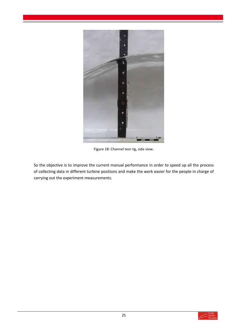
25
Figure 18: Channel test rig, side view.
So the objective is to improve the current manual performance in order to speed up all the process
of collecting data in different turbine positions and make the work easier for the people in charge of
carrying out the experiment measurements.

26

27
3 Objectives
After considering the main problems of the current Measurement and Turbine Concepts, it is
necessary to make a Functional Specific Document.
A Functional Specific Document is a document which reflects the different objectives, which
will be necessary to achieve at the end of the Thesis, this document reflects not only the
objectives but also some extra information which is important for understanding all the
requirements that the chosen concepts should have.
Table 1 is divided in two parts: On the one hand the Measurement Concept in order to
improve the current measurement system due to its lack of accuracy and on the other hand a
Turbine Concept where it is important to make the turbine operating and removing systems
automatically instead of manually.
Note that in the part of the Measurement concept that the pressure calculated, is the static
one, so if the water level is known with the following formula we can easily get the pressure.
𝑝𝑠 = 𝜌𝑔ℎ (Eq. 20)
Some other formulas used at the time of filling Table 1 were:
𝜎 =𝐴
𝑏·𝐻1 (Eq. 21)
휁 =𝑍
𝐻1 (Eq. 22)
𝛼(𝑥) =𝐴𝑡(𝑥)
𝑏·𝐻1 (Eq. 23)
𝑍𝑡(𝑥) =𝑍𝑡(𝑥)
𝐻1 (Eq. 24)
Eq. 21 and Eq.22 represents the ratio of the turbine width and height, whereas Eq.23 and Eq.24
represents the ratio of the width and the medium line of the streamtube generated by the turbine.
By knowing that b = 0.2 m and 𝐻1= 0.25 m, the ranges shown at Table 1 were calculated.
The velocity range written in the table has been done with Froude Numbers between 0.2-1.4 which is
the range that we are working with along the channel. (See Eq. 19)
The Factor 1.3 previously explained is added when calculating velocities closely to the turbine.

28
Table 1: Functional Specific Document
Concepts
Require
ments
Sym
bol
Poin
ts o
f Measure
ment
Range
Typ
e o
f Info
rmatio
nE
xtra In
form
atio
n
Concept M
easure
ment
Measure
velo
city
u0.3
5-1
.68 m
/sB
F
u(x,y)
0.3
5-1
.68 m
/sB
FD
istrib
utio
n b
etw
een 1
and 2
u(x,y)
0.3
5-1
.68 m
/sW
Dis
tributio
n b
etw
een 2
and 3
Measure
Pre
ssure
p980-3
920 P
aB
F
p(x)
980-3
920 P
aB
FD
istrib
utio
n b
etw
een 1
and 2
p(x)
980-3
920 P
aW
Dis
tributio
n b
etw
een 2
and 3
Mesure
wate
r leve
lh
0.1
-0.4
mB
F
h(x,z
)0.1
-0.4
mB
FD
istrib
utio
n b
etw
een 1
and 2
h(x,z
)0.1
-0.4
mW
Dis
tributio
n b
etw
een 2
and 3
Measure
of th
e w
idth
of th
e S
tream
tube
α(x)
Turb
ine to
20.2
-1B
FD
istrib
utio
n b
etw
een 1
and 2
Measure
Mediu
m lin
e o
f the S
tream
tube
ƺ(x)
Turb
ine to
20.1
-1B
FD
istrib
utio
n b
etw
een 1
and 2
Measure
of th
e w
idth
of th
e S
tream
tube
Turb
ine to
20.0
1-0
.05
BF
Dis
tributio
n b
etw
een 1
and 2
Measure
Mediu
m L
ine o
f the S
tream
tube
Turb
ine to
20.0
25-0
.25m
BF
Dis
tributio
n b
etw
een 1
and 2
Econom
ical L
imita
tions
WM
ate
rial a
vaila
ble
in T
U D
arm
sta
dt
Concept T
urb
ine
Turb
ine w
idth
σ
Turb
ine
0.2
-1B
F
Turb
ine h
eig
ht
ƺT
urb
ine
0.1
-1B
F
Turb
ine w
idth
A
Turb
ine
0.0
1-0
.05
BF
Turb
ine h
eig
ht
ZT
urb
ine
0.0
25-0
.25 m
BF
Num
ber o
f Turb
ine w
idth
# σ
Turb
ine
4+
BF
Num
ber o
f Turb
ine h
eig
ht
# ƺ
Turb
ine
4+
BF
Diffe
rent R
esis
tances
RT
urb
ine
3+
BF
Econom
ical L
imita
tions
WM
ate
rial a
vaila
ble
in T
U D
arm
sta
dt
𝑢1
𝑢+
𝑢−
𝑢2
𝑢3
ℎ1
ℎ+
ℎ−
ℎ2
ℎ3
𝐴𝑡 (𝑥
)
𝑍𝑡 (𝑥
)𝑚
2
𝑚2
𝑝1
𝑝+
𝑝−
𝑝2
𝑝3

29
BF: Fixed Requirement for a determined range
W: Wish
The points of measurement (1), (+), (-), (2) and (3) are referred to the Figure 2.
To sum up, the main objectives are:
Measurement concept:
Measure velocity
Measure water level altimetry and static pressure
Measure the medium line and the width of the streamtube
Turbine Concept
Automatic change of turbine height position
Easier change and election of the turbine resistances
Easier change of turbines size

30

31
4 Research
The research of the measurement concept is divided in two parts: Velocity Measurements (4.1.) and
the Water Level Measurements (4.2.).
4.1 Velocity Measurements
The first step, in the measurement concept, has been a research of possible techniques for the
velocity measurement. They have been placed in Table 2 in order to compare them and analyse if
they achieve the objectives of the Measurement Concept.
Table 2: Evaluation of Velocity Measurement Techniques
PIV
P
TV
Pito
tM
ulti-h
ole
Pro
be
Ho
t Wire
Pro
be
LD
AM
TV
Flo
w V
isu
aliz
atio
n
AY
ES
YE
SY
ES
YE
SY
ES
Partia
llyY
ES
YE
S
u (c
ascad
e)
YE
SY
ES
NO
NO
YE
SY
ES
YE
SY
ES
u (re
st)
YE
SY
ES
YE
SY
ES
YE
SN
OY
ES
YE
S
h (c
ascad
e)
NO
NO
NO
NO
NO
NO
NO
NO
h (re
st)
NO
NO
YE
SY
ES
NO
NO
NO
NO
zY
ES
YE
SY
ES
YE
SY
ES
Partia
llyY
ES
YE
S
p (c
ascad
e)
Partia
llyP
artia
llyN
OP
artia
llyP
artia
llyP
artia
llyP
artia
llyP
artia
lly
p (re
st)
Partia
llyP
artia
llyY
ES
YE
SP
artia
llyN
OP
artia
llyP
artia
lly
Eco
no
mic
NO
NO
YE
SM
ediu
mY
ES
NO
NO
YE
S
Accu
racy
Hig
hH
igh
Mediu
mM
ediu
mM
ediu
mH
igh
Hig
hN
O
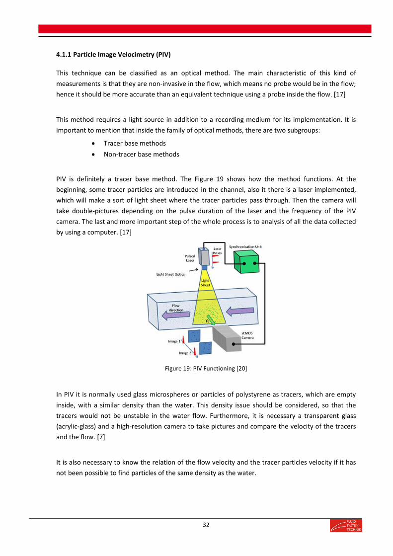
32
4.1.1 Particle Image Velocimetry (PIV)
This technique can be classified as an optical method. The main characteristic of this kind of
measurements is that they are non-invasive in the flow, which means no probe would be in the flow;
hence it should be more accurate than an equivalent technique using a probe inside the flow. [17]
This method requires a light source in addition to a recording medium for its implementation. It is
important to mention that inside the family of optical methods, there are two subgroups:
Tracer base methods
Non-tracer base methods
PIV is definitely a tracer base method. The Figure 19 shows how the method functions. At the
beginning, some tracer particles are introduced in the channel, also it there is a laser implemented,
which will make a sort of light sheet where the tracer particles pass through. Then the camera will
take double-pictures depending on the pulse duration of the laser and the frequency of the PIV
camera. The last and more important step of the whole process is to analysis of all the data collected
by using a computer. [17]
Figure 19: PIV Functioning [20]
In PIV it is normally used glass microspheres or particles of polystyrene as tracers, which are empty
inside, with a similar density than the water. This density issue should be considered, so that the
tracers would not be unstable in the water flow. Furthermore, it is necessary a transparent glass
(acrylic-glass) and a high-resolution camera to take pictures and compare the velocity of the tracers
and the flow. [7]
It is also necessary to know the relation of the flow velocity and the tracer particles velocity if it has
not been possible to find particles of the same density as the water.
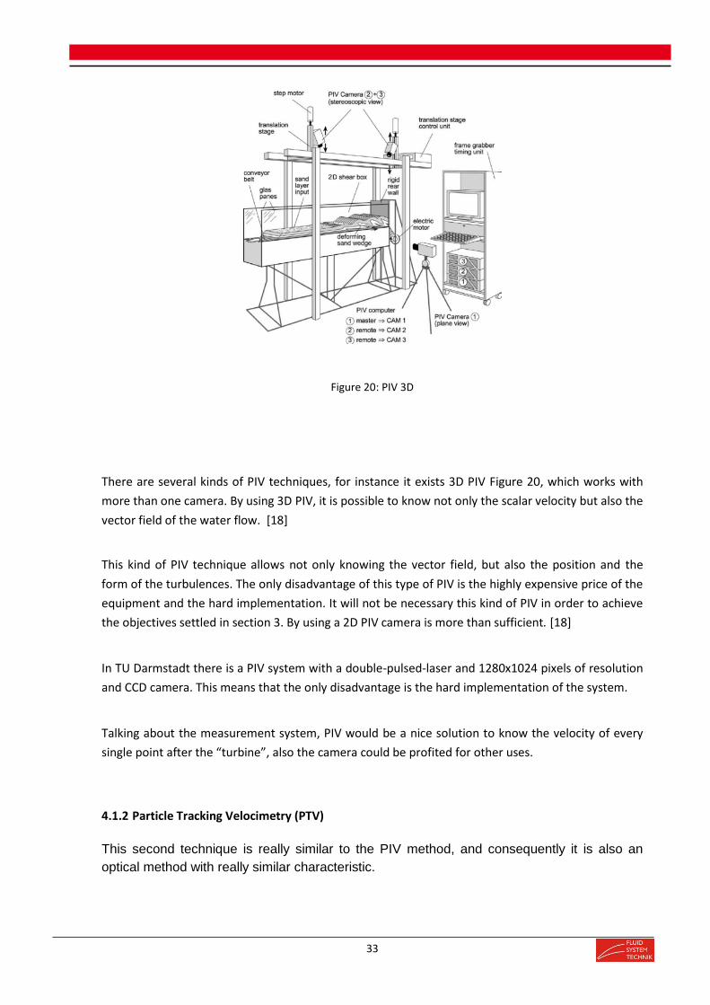
33
Figure 20: PIV 3D
There are several kinds of PIV techniques, for instance it exists 3D PIV Figure 20, which works with
more than one camera. By using 3D PIV, it is possible to know not only the scalar velocity but also the
vector field of the water flow. [18]
This kind of PIV technique allows not only knowing the vector field, but also the position and the
form of the turbulences. The only disadvantage of this type of PIV is the highly expensive price of the
equipment and the hard implementation. It will not be necessary this kind of PIV in order to achieve
the objectives settled in section 3. By using a 2D PIV camera is more than sufficient. [18]
In TU Darmstadt there is a PIV system with a double-pulsed-laser and 1280x1024 pixels of resolution
and CCD camera. This means that the only disadvantage is the hard implementation of the system.
Talking about the measurement system, PIV would be a nice solution to know the velocity of every
single point after the “turbine”, also the camera could be profited for other uses.
4.1.2 Particle Tracking Velocimetry (PTV)
This second technique is really similar to the PIV method, and consequently it is also an
optical method with really similar characteristic.
34
This method is normally used in order to measure the velocity of particles that are inside a flow,
tracer base method, usually it is used a CCD Camera in order to make the pictures in order to analyse
the behaviour of the tracer particles in the flow. [18]
There are some differences between PTV and PIV. In PTV individual particles are tracked, that means
that it follows a Lagrangian approach, whereas in PIV the approach is Eulerian and consequently the
density of tracer particles in PTV is so much lower than in PIV. If there are less tracer particles, there
are also lower vector fields. [21]
One advantage of PTV is that apart from the vector field of the velocity we can know the streamtube
shape, which would be great information for the thesis because two of the objectives are measuring
the width and the medium line of the streamtube.
As well as in PIV, there are two methods of measuring in PTV:
2D-PTV where we measure the flow field in two dimensions by illuminating with a laser sheet
and with lower quantity the particles than in PIV we can track each particle individually for
some frames.
3D-PTV is based on several cameras, 3-dimensional illumination and tracking of flow tracers,
which can be also different from solid particles, this technique is based on photogrammetric
principles.
A common 3D-PTV consists of several digital cameras, usually three or four, with an angular
installation. These cameras should be synchronous recording the light from the tracers particles in
the water flow. As in PIV the flow is illuminated by a laser, the light has not restriction, which means
that it can be coherent, monochromatic, etc. It is worth bearing in mind that the more consecutive
frames that the particles are tracked, the better for the experiment. [21]
In the current case, it is not necessary the accuracy of 3D-PTV, so 2D-PTV would be quite enough.
PTV is a great solution for the improvement of the measurement system. It would help not only to
know the velocity in each point but also the shape of the streamtube, which is also an important
requirement. The implementation and the costs will be discussed in the section 4.2.
4.1.3 Pitot Tube
This type of technique focuses in a pressure measurement; thanks to this instrument it is possible to
know the dynamic pressure 𝑝𝑡. [8]

35
𝑝𝑡 =1
2𝜌𝑢2 (Eq. 25)
It is a really common method of measuring in aerodynamic and hydraulic applications, however it
carries with some problems of accuracy when the flow is unstable. In this particular case, it is worked
with waves produced by the turbine, and consequently there will be a superposition between the
static pressure and the dynamic pressure, if the probe is not placed perpendicular to the surface.
In this technique there is influence of some parameters such as the measured difference of pressure,
the pipe geometry, surface tension, trapped air mass and the temperature as it can be seen in the
calculations made by M.Lehr. [8]
𝑝𝑡 =𝑚𝑎𝑖𝑟·𝑅𝑠·𝑇
𝑉−
2𝑠
𝑅− 𝜌𝑔𝑥 (Eq. 26)
Figure 21: Pitot Tube
Although it has some problems of accuracy, one of the requirements is to know the velocity
before the turbine, in this part of the test rig would be a good idea to use a Pitot tube due to
the fact that it is already implemented in the laboratory.
4.1.4 Multi-hole Probe
This technique is a concept really similar to the Pitot tube, but extended to a more than one
dimension. The holes could be between three and seven depending on the type of the probe. The
more holes the probe has, the better measurements would be done in the other directions. [22]
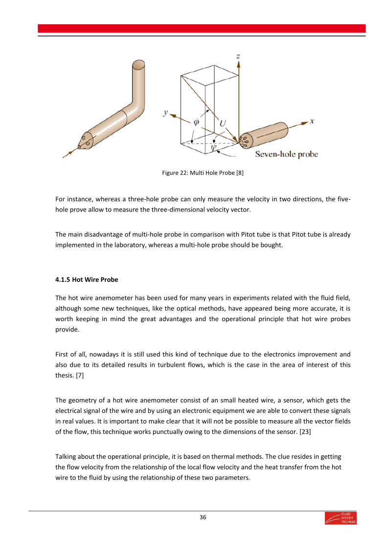
36
Figure 22: Multi Hole Probe [8]
For instance, whereas a three-hole probe can only measure the velocity in two directions, the five-
hole prove allow to measure the three-dimensional velocity vector.
The main disadvantage of multi-hole probe in comparison with Pitot tube is that Pitot tube is already
implemented in the laboratory, whereas a multi-hole probe should be bought.
4.1.5 Hot Wire Probe
The hot wire anemometer has been used for many years in experiments related with the fluid field,
although some new techniques, like the optical methods, have appeared being more accurate, it is
worth keeping in mind the great advantages and the operational principle that hot wire probes
provide.
First of all, nowadays it is still used this kind of technique due to the electronics improvement and
also due to its detailed results in turbulent flows, which is the case in the area of interest of this
thesis. [7]
The geometry of a hot wire anemometer consist of an small heated wire, a sensor, which gets the
electrical signal of the wire and by using an electronic equipment we are able to convert these signals
in real values. It is important to make clear that it will not be possible to measure all the vector fields
of the flow, this technique works punctually owing to the dimensions of the sensor. [23]
Talking about the operational principle, it is based on thermal methods. The clue resides in getting
the flow velocity from the relationship of the local flow velocity and the heat transfer from the hot
wire to the fluid by using the relationship of these two parameters.

37
Figure 23: Measurement principles of CTA [23]
In the hot wire anemometer, two different systems can be used: CCA (Constant Current) and CTA
(Constant Temperature).
In the current case it is preferable to use the Constant Temperature Anemometer for our test rig
than the CCA, the circuit would be like the following one:
Figure 24: Circuit of a hot wire probe [24]
Using the CTA system implies providing a controlled amount of electrical current, whereas
maintaining the wire temperature constant, implies a variation of the heat transfer.

38
Figure 25: Operation principle of a hot wire probe [22]
It is also important to talk about the sensor that it is used in this method, it is said that a proper
sensor for a hot wire anemometer need the following characteristics: [23]
High value of the temperature coefficient resistance.
An electrical resistance, which can be heated with a common voltage and current levels.
Small size of the wire.
High resistance in order to resist the stresses of the hydraulic flow.
The most common hot wire sensor is the tungsten coated with a thin platinum layer. It provides a
much more resistance to oxidation. [24]
There are plenty of different types of probes. In Figure 26 are shown the three types of probe more
relevant, which are the most popular in our field of measurement. [23]
Figure 26: Different Types of Hot Wire Probes [23]
In the left picture it can be observed a Fiber-film probe, in the central picture a X-wire probe and in
the right side a tri-axial probe for 3D-flows.
This method can be used either in air or in water, in this thesis it is worked in water so in order to
perverse the quartz coating, it is necessary to make sure that grounding water takes place. In this
case we protect the hot wire from damage due to voltage differences. [23]
The last important point about this technique is the calibration, it is possible to do a calibration in-
situ in the test rig, but it would be really complicated, so usually it is done in another canal.
4.1.6 Laser Doppler Anemometry
LDA is a tool used in many fluid dynamic investigations in gases or liquids in order to know the flow
velocity. As well as PIV or PTV is an optical method with a non-intrusive principle, it is also necessary
some tracer particles. [27]
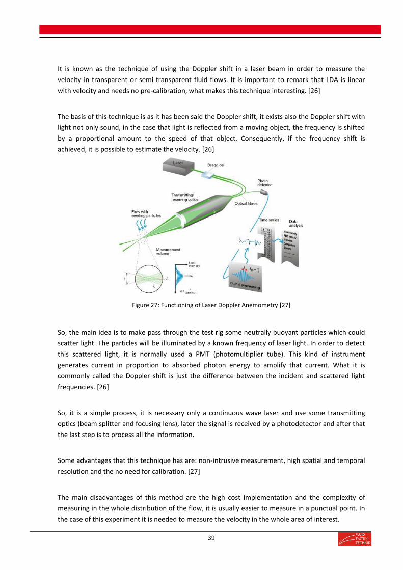
39
It is known as the technique of using the Doppler shift in a laser beam in order to measure the
velocity in transparent or semi-transparent fluid flows. It is important to remark that LDA is linear
with velocity and needs no pre-calibration, what makes this technique interesting. [26]
The basis of this technique is as it has been said the Doppler shift, it exists also the Doppler shift with
light not only sound, in the case that light is reflected from a moving object, the frequency is shifted
by a proportional amount to the speed of that object. Consequently, if the frequency shift is
achieved, it is possible to estimate the velocity. [26]
Figure 27: Functioning of Laser Doppler Anemometry [27]
So, the main idea is to make pass through the test rig some neutrally buoyant particles which could
scatter light. The particles will be illuminated by a known frequency of laser light. In order to detect
this scattered light, it is normally used a PMT (photomultiplier tube). This kind of instrument
generates current in proportion to absorbed photon energy to amplify that current. What it is
commonly called the Doppler shift is just the difference between the incident and scattered light
frequencies. [26]
So, it is a simple process, it is necessary only a continuous wave laser and use some transmitting
optics (beam splitter and focusing lens), later the signal is received by a photodetector and after that
the last step is to process all the information.
Some advantages that this technique has are: non-intrusive measurement, high spatial and temporal
resolution and the no need for calibration. [27]
The main disadvantages of this method are the high cost implementation and the complexity of
measuring in the whole distribution of the flow, it is usually easier to measure in a punctual point. In
the case of this experiment it is needed to measure the velocity in the whole area of interest.
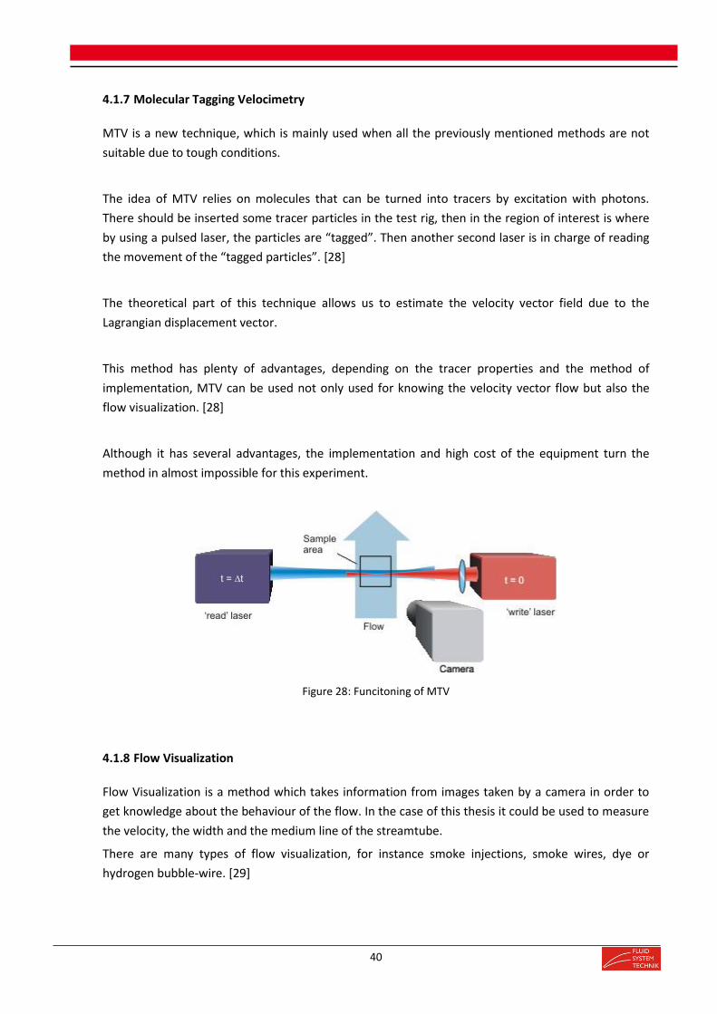
40
4.1.7 Molecular Tagging Velocimetry
MTV is a new technique, which is mainly used when all the previously mentioned methods are not
suitable due to tough conditions.
The idea of MTV relies on molecules that can be turned into tracers by excitation with photons.
There should be inserted some tracer particles in the test rig, then in the region of interest is where
by using a pulsed laser, the particles are “tagged”. Then another second laser is in charge of reading
the movement of the “tagged particles”. [28]
The theoretical part of this technique allows us to estimate the velocity vector field due to the
Lagrangian displacement vector.
This method has plenty of advantages, depending on the tracer properties and the method of
implementation, MTV can be used not only used for knowing the velocity vector flow but also the
flow visualization. [28]
Although it has several advantages, the implementation and high cost of the equipment turn the
method in almost impossible for this experiment.
Figure 28: Funcitoning of MTV
4.1.8 Flow Visualization
Flow Visualization is a method which takes information from images taken by a camera in order to
get knowledge about the behaviour of the flow. In the case of this thesis it could be used to measure
the velocity, the width and the medium line of the streamtube.
There are many types of flow visualization, for instance smoke injections, smoke wires, dye or
hydrogen bubble-wire. [29]

41
Another option could be to position some foils at the upper and bottom part of the perforated plate
as it is shown in Figure 29. The idea of this concept resides in measuring the distance of the foils
which consists in the width of the streamtube.
As the volume flow which is passing through the perforated plate is constant, by knowing the
distribution of the distance between the foils. It is trivial to calculate the velocity of the flow which
has passes through the turbine by using Eq. 27.
Also it would be necessary to measure the velocity in the entrance of the perforated plate, this
velocity could be measured by using a Pitot tube or a hot wire anemometry, which have been
explained before.
𝑄𝑡𝑢𝑟𝑏𝑖𝑛𝑒 = 𝑢 · 𝐴𝑠𝑡𝑟𝑒𝑎𝑚𝑡𝑢𝑏𝑒 (Eq. 27)
It is worth bearing in mind that the velocities of the water flow from the by-pass flow and the water
flow which passes through the turbine are different; this means that the volume flow, which passes
through the turbine, is going to remain constant until the mixing zone see Figure 2. Just by knowing
the area of the stream tube in each point it is easy to know the velocity between the points (-) and
(2).
One of the very first ideas was to use foils of polyethylene with bands of polystyrene, which will fit
together with the “turbines” in order to visualize the streamtube of the flow like in Figure 29. It was
decided to use this material because it has a density similar to water, it is totally necessary to work
with materials with the same density as water in order to have a stable prototype. The main
problems of using this kind of foils will be commented in section 4.2.
Figure 29: Flow visualization with foils.

42
The other type of Flow Visualization, which has been studied in this thesis, has been Hydrogen
Bubble generation. The technique relies on the generation of hydrogen bubbles by electrolysis, the
hydrogen bubbles are produces in a thin wire (25-50 μm), which acts as the cathode of the DC circuit.
The anode terminal of the circuit is commonly a metal located in the bottom part of the channel. [30]
Note that the wire should be the cathode in order to generate small hydrogen bubbles. If the anode
is the one chosen, oxygen bubbles would be generated instead of hydrogen bubbles. Generally
oxygen bubbles are not desirable because they normally nucleate easily, and have larger size than
the hydrogen bubbles, which are around half size the wire diameter. [31]
Although the hydrogen bubbles have not the same density as water, as the wires are really small in
size, the buoyancy forces are negligible in comparison with the drag forces, this fact means that the
bubbles will not produce a disturbance of the flow conditions.
Figure 30: Hydrogen Bubble
One of the most important advantages of this technique is its versatility; they can be located almost
anywhere. Other good points of this method are simplicity, quick experimentation and cost
effectiveness. [32]
On the other hand, this method has some limitations, the principal one relies on its effectiveness for
low Reynold numbers. In our case maximum Reynolds number, which occurs in the cascade with
𝐹𝑟 = 1.4 and 𝑄 = 82m3/𝑠 (worst case) is approximately 𝑅𝑒 = 2.6 · 105. This means turbulent flow
and leads to some necessary calibrations and dimensions of the wire, which will be commented in
section 4.2.

43
If the flow is turbulent, it is normally used wires probes of 25-50 μm because the diameter of the
bubbles is directly proportional to the diameter of the wire. In turbulent flow it is necessary to use
low bubble diameter in order to have a nice visualization. Wire probes larger than 50 μm will lead to
poor quality visualization. However, the smaller the wire is, the more possibilities of breakage of the
wire. [33]
Another important limitation is the high degree of trial and error involved, the calibration is really
tough. In fact after calibration it is possible to visualize complex flows successfully.
The system of hydrogen bubble generation consists of a DC-power supply, with a voltage range of
minimum 70 V, this voltage depends on other parameters which will be discuss later, a current
capacity of at least 1 A. In order to create DC voltage can be used a transformer and rectifier.
Another possibility is an off-the-shelf switching power supply. [34]
It is also necessary to have a pulse generator which enables to measure the local velocity by creating
series of time lines of hydrogen bubbles. It will be detailed in section 5.2.
It should be noticed that a safety system is necessary when working with this method, contact with
the wire probe, the anode or the water flow can result extremely dangerous. Typically is used a
circuit breaker to limit the electrical current. [33]
It is important to notice that the bubbles which are generated in the wake of a bubble wire move a
little bit slower than the local velocity due to the wake effect of the wire, which can be quantitatively
account as did Lu & Smith (1991) [35]
Normally salts are added to tap water, which contains dissolved electrolytes to facilitate a good
electrolytic process, for instance common salt, sodium sulphate or hydrochloric acid. It is important
that there is not a big concentration of electrolytes in order to avoid nucleation of the bubbles at
lower voltage levels and corrosion of metals. [32]
Talking about the wires, it is necessary to comment that wires often fail (wire breaks), one has to be
skilled when constructing this kind of structures. There are different types of wires: horizontal and
vertical as it can be observed in Figure 31.
As it has been previously mentioned conductive wires consists of 25-50 μm welded between two
metal and conductive supports as it can be observed in Figure 31. It is necessary that the wire is
under tension to provide a clean sheet of bubbles, however too much tension will result on the
breakage of the wire. The material, geometry and insulation of the wire probe and the supporting
parts will be discussed in section 5.2.

44
Figure 31: Types of wire probes [32]
Another common problem is the contamination of electrolytes produced on the wire, which can be
cleaned by momentary reversal of the electrical polarity by the incorporation of a switch in the
power supply circuit. It is necessary to “clean” the wire for approximately 8 seconds with an
operating voltage lower than 50 V. [33]
Illumination is necessary in hydrogen bubbles generation to create a clear visualization of the flow
and consequently nice pictures which can be analysed. A high-power light emitting diode (LED) is
effective. It is available and provides light output like common lamps with small power requirements
and infrared emissions. In section 5.2 will be commented the positioning of the LEDs in the test
channel. It is also used a contrast background in order to improve the image quality. A simple
solution is the usage of a black poster board behind the area photographed. [32]
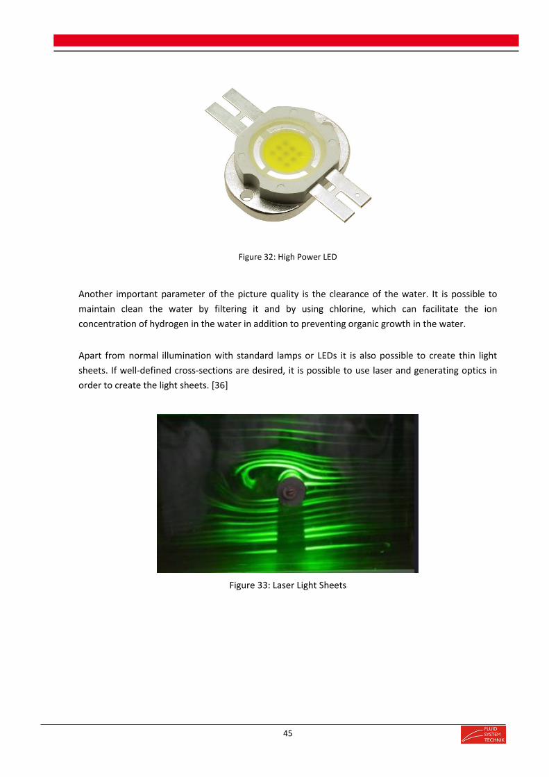
45
Figure 32: High Power LED
Another important parameter of the picture quality is the clearance of the water. It is possible to
maintain clean the water by filtering it and by using chlorine, which can facilitate the ion
concentration of hydrogen in the water in addition to preventing organic growth in the water.
Apart from normal illumination with standard lamps or LEDs it is also possible to create thin light
sheets. If well-defined cross-sections are desired, it is possible to use laser and generating optics in
order to create the light sheets. [36]
Figure 33: Laser Light Sheets

46
4.2 Water Level Measurements
In this part of the project, it has been found eight possible techniques in order to measure the
water level altimetry of the flow. As it has been done in section 4.1., all the possible
techniques have been placed in a table with the parameters which need to be measured.
Table 3: Evaluation of the Water level Measurement techniques
4.2.1 Camera
This might be one of the simplest methods of the level water measurement, it consists just in
taking a lot of pictures of the area of interest with a high resolution camera, or even with a
Cam
era
Laser
Co
nd
uctive
Leve
l Altim
etry
Cap
acitive Le
vel A
ltime
tryD
irect M
easu
rem
en
tU
ltrason
icR
adar
Mag
ne
tostric
tive
Le
ve
l Tra
nsm
itters
AN
ON
ON
ON
ON
ON
ON
ON
O
u (cascad
e)
NO
NO
NO
NO
NO
NO
NO
NO
u (re
st)N
ON
ON
ON
ON
ON
ON
ON
O
h (cascad
e)
YESYES
YESP
artYES
YESYES
YES
h (re
st) YES
YESYES
YESYES
YESYES
YES
zN
ON
ON
ON
ON
ON
ON
ON
O
p (cascad
e)
Part
Part
Part
Part
Part
Part
Part
Part
p (re
st)P
artP
artP
artP
artP
artP
artP
artP
art
Econ
om
icYES
NO
YESN
OYES
Me
diu
mM
ed
ium
NO
Accu
racyM
ed
ium
High
Me
diu
mM
ed
ium
Low
High
Me
diu
mH
igh
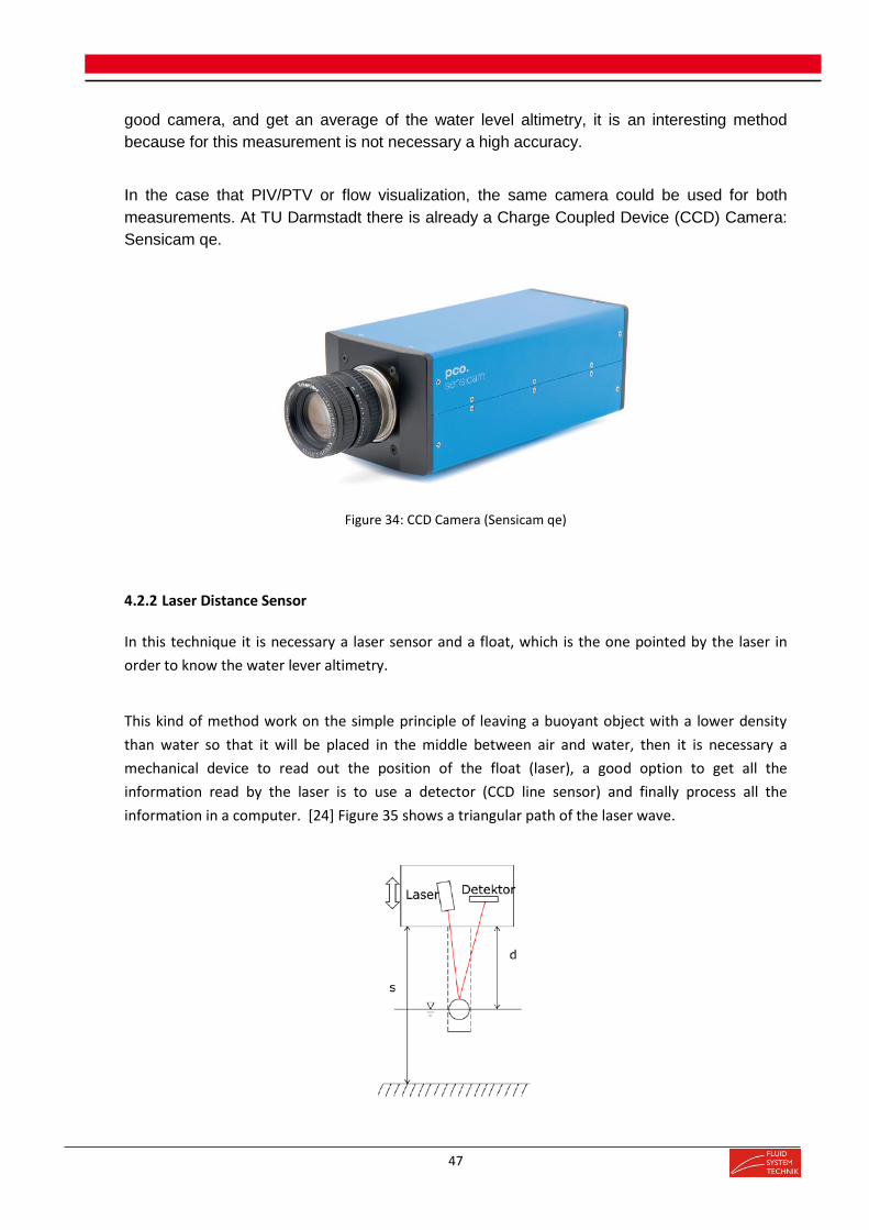
47
good camera, and get an average of the water level altimetry, it is an interesting method
because for this measurement is not necessary a high accuracy.
In the case that PIV/PTV or flow visualization, the same camera could be used for both
measurements. At TU Darmstadt there is already a Charge Coupled Device (CCD) Camera:
Sensicam qe.
Figure 34: CCD Camera (Sensicam qe)
4.2.2 Laser Distance Sensor
In this technique it is necessary a laser sensor and a float, which is the one pointed by the laser in
order to know the water lever altimetry.
This kind of method work on the simple principle of leaving a buoyant object with a lower density
than water so that it will be placed in the middle between air and water, then it is necessary a
mechanical device to read out the position of the float (laser), a good option to get all the
information read by the laser is to use a detector (CCD line sensor) and finally process all the
information in a computer. [24] Figure 35 shows a triangular path of the laser wave.

48
Figure 35: Functioning of the Laser Distance Sensor [29]
By knowing the position of the laser and detector (s) and the distance between the detector and the
surface (d) it is possible to get the water level height (h). This is a basic explanation; a further
explanation of this method can be found in reference [8]
ℎ = 𝑠 − 𝑑 (Eq. 28)
If we get in detail, the laser diode produces a dot in the float, this light is scattered, and it passes
through some lens to finally arrive to the sensor (detector). The measurement error in this kind of
triangular sensor methods is less than 0.1 mm. [37]
Some advantages of this technique are the high accuracy, the low invasiveness, acceptable price and
easy implementation. [37]
The main disadvantages are the difficult functioning of this method in the cascade, which generates
much turbulence and the difficulty of passing over the turbine. This fact lead to the rejection of this
concept.
4.2.3 Conductive Level Altimetry
As it was previously explained in section 2.3 this method is currently used to measure the conductive
level altimetry. The operational system depends on the electrical conductivity between two
electrodes, which is function the filling height of the test rig.
So in this method it is used a needle electrode in order to scan the surface and achieve the level
height. The theoretical property that is used is that the electrical conductivity of the water is much
higher than the one from the air. [37]

49
Figure 36: Scheme of the Conductive Level Altimetry method [8]
The geometry of the measurement system can be observed in Figure 36. It consists of a fixed
electrode already immersed in water. The sensing electrode is moved perpendicular to the water
surface with a stepper motor and a ball screw. At the moment that the needle electrode touches the
water the electric flow is detected and consequently the water level altimetry of the test rig, if the
needle electrode does not touch the water there would not be an electrical continuity. [37]
This measurement has an important disadvantage, the large invasiveness of the method; this fact
provides a lower accuracy than other methods. Other students did some tests about this technique
and there were large scattering at the cascade point, which is the area of interest, see section 2.3. [8]
4.2.4 Capacitive Level Altimetry
The operational principle of this technique resides in the fact that the capacitance of a capacitor is a
function of the relative permittivity, which is quite different in the water than in the air. By using this
property it is possible to calculate the water level by using the following formula: [9]
𝐶𝑡𝑜𝑡𝑎𝑙(ℎ) = 𝜖0𝑏
𝑑(휀𝑟,𝑎𝑖𝑟 · 𝐿 + (휀𝑟,𝐻2𝑂 − 휀𝑟,𝑎𝑖𝑟) · ℎ) (Eq. 29)
Figure 37: Description of Capacitive Level Altimetry method [29]
After some calculations done in [9], it is achieved the asset that this technique is not that accurate for
commercial capacitor up to 1 𝑝𝐹, hence it would be necessary to buy special capacitor, so much
more expensive.
In this measurement systems there are a few aspects that should be considered, for instance there is
a problem with the fluctuations of the temperature, it is important to consider this fact because the

50
relative permeability changes a lot with the temperature. This is not a problem due to the constant
temperature of the laboratory were the test rig is placed.
Another important aspect to comment is the capillary, if we use a big invasive sensor, it will make the
water level rise in the gap between the electrodes of the capacitor. Here there are two options:
Use a smaller sensor with the disadvantage of requiring a capacitor with lower capacitance,
which means more expensive.
Use a big sensor assuming that there could appear the capillary phenomena.
To sum up, it will not be one of the most suitable techniques for the experiment due to the large
invasiveness and the high cost of the special capacitors. Also the measurement will not be really
accurate in the area of interest.
4.2.5 Direct Measurement
This method is the simplest one and also the least accurate. It consists just in measuring with a
normal ruler in a transparent glass the water level of the test rig. It is not a measurement that we
should consider seriously. The lack of accuracy is too high so this technique should be rejected
because there are so many options better than this one.
4.2.6 Ultrasonic Level Transmitter
This technique measures the water level altimetry by using ultrasonic waves. The idea is to measure
the distance between the transducer and the water surface by using the ultrasonic pulse, which
travels from the transducer to the surface and comes back, (TOF). [38]
Figure 38: Ultrasonic Measurement [38]

51
Figure 38 explains graphically how the system works. These systems works perfectly for flat surfaces
like a tank, but in a cascade the accuracy is not that high. Another disadvantage is the possible false
echoes of the walls or the structures that could appear. As the area of interest is not flat, this method
should be rejected. [38]
4.2.7 Radar Level Altimetry
This technique requires an air radar system beam microwaves downward from an antenna, which
will be placed at the top of the test rig.
The idea is that the signal provided form the transmitter is reflected off the liquid surface back to the
antenna, by knowing the timing circuit it is possible to calculate the distance to the fluid surface by
measuring the round-trip time (TOF).[38]
Figure 39: Radar Level Altimetry measurement
This method could have measurement problems if the dielectric constant of the fluid is low, the
reason of this fact is that the amount of reflected energy frequencies depends on the dielectric
constant. If it is low, it means that the radar’s energy enters or passes through. In our case, water
(휀𝑟 = 80) there are no continuity problems. [38]
Some other problems related to this system are the divergence of the beam that could provide
erroneous readings. In order to overcome this problem, it can be incorporated complex algorithms
using fuzzy logic to the transmitter, although this is not a simple solution, another simplest solution
could be to use Guided Waver Radar (GWR) systems, it consists of a flexible cable antenna system,
which guides the microwave down from the top of the test rig to the surface water and back to the
transmitter, this system is 20 times more efficient that normal radar systems [38]
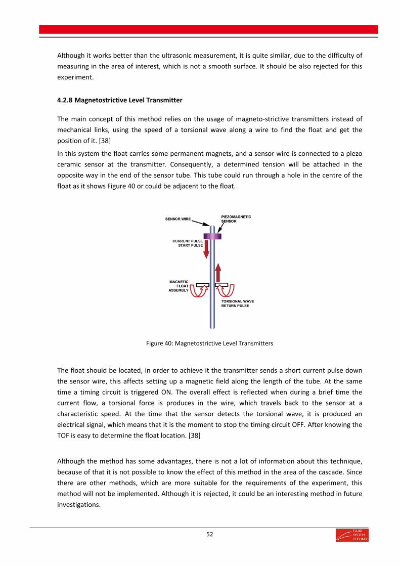
52
Although it works better than the ultrasonic measurement, it is quite similar, due to the difficulty of
measuring in the area of interest, which is not a smooth surface. It should be also rejected for this
experiment.
4.2.8 Magnetostrictive Level Transmitter
The main concept of this method relies on the usage of magneto-strictive transmitters instead of
mechanical links, using the speed of a torsional wave along a wire to find the float and get the
position of it. [38]
In this system the float carries some permanent magnets, and a sensor wire is connected to a piezo
ceramic sensor at the transmitter. Consequently, a determined tension will be attached in the
opposite way in the end of the sensor tube. This tube could run through a hole in the centre of the
float as it shows Figure 40 or could be adjacent to the float.
Figure 40: Magnetostrictive Level Transmitters
The float should be located, in order to achieve it the transmitter sends a short current pulse down
the sensor wire, this affects setting up a magnetic field along the length of the tube. At the same
time a timing circuit is triggered ON. The overall effect is reflected when during a brief time the
current flow, a torsional force is produces in the wire, which travels back to the sensor at a
characteristic speed. At the time that the sensor detects the torsional wave, it is produced an
electrical signal, which means that it is the moment to stop the timing circuit OFF. After knowing the
TOF is easy to determine the float location. [38]
Although the method has some advantages, there is not a lot of information about this technique,
because of that it is not possible to know the effect of this method in the area of the cascade. Since
there are other methods, which are more suitable for the requirements of the experiment, this
method will not be implemented. Although it is rejected, it could be an interesting method in future
investigations.

53
5 Measurement Concept
5.1 Election of the Concept
After explaining all the possible techniques that have been researched, the election of the concept
for the measurement system will be explained in this section of the project. The following three
combinations have been chosen due to the fact that they achieve the requirements of the concept
settled in section 3.
1. Pitot Tube + Conductive Level Altimetry
2. Flow Visualization + Camera + Pitot Tube
3. PIV/PTV + Camera
5.1.1 Pitot Tube + Conductive Level Altimetry
This combination is the current state of the project, the velocity is measured by a Pitot tube, which it
is already implemented in the laboratory, and the water lever measurement is measured with the
Conductive level altimetry.
The main reasons because of that this current combination is rejected have been already explained
in sections 2.3., 4.1.3 and 4.2.3.
In light of the above mentioned, it is necessary to say that this option is the worst one of the three
proposed due to its lack of accuracy.
5.1.2 Flow Visualization + Pitot tube + Camera
In the second combination, the velocity would be measured with the previous mentioned technique:
flow visualization + Pitot tube and the water level measurement would be measured by a high
resolution camera.
The high resolution camera used for the water level measurement will be the same one which is
going to be used for the flow visualization technique, which as it has been before commented, it is
available in TU Darmstadt.
5.1.2.1 Polyethylene Foils Concept
This concept was commented in section 4.1.8., it was the very first idea for the flow visualization.
After researching different materials which were solid, flexible and had a similar water density (1 𝑔/

54
𝑐𝑚3), there were found two options: Low Density Polyethylene (LDP), which has a density
between (0.92 − 0.94 𝑔/𝑐𝑚3) and High Density Polyethylene (HDP), which has a density
between (0.93 − 0.97 𝑔/𝑐𝑚3) .
Although HDP has a more similar density to the water, the elected material was LDP due to its
flexibility. After validating LDP, it can be said that LDP is enough stable in the water, which means
that the foils were not sinking nor floating.
Some bands of polystyrene (0.96 − 1.04 𝑔/𝑐𝑚3) were added to the polyethylene foils in order to
make them more consistent and heavier.
The foils will be coupled in the following assembly:
Figure 41: Turbine Structure
The assembly is formed by two pieces called foils support, the turbine support and four pieces (3).
Each foil support is coupled to the turbine support by two pieces (3), through the holes there will be
a screw fixing the elements.

55
The foils will be fixed to the foils support, as it can be observed in Figure 29, and it won’t be
necessary to remove then when changing the size of the turbine. So, the good point of this concept
structure resides in the fact that when using perforated plates with different width, it will be only
necessary to screw the foils support to a different hole of the turbine support.
It will only be necessary to screw when changing the size of the turbine, but not when changing the
type of resistance of the perforated plate, which is quite interesting in order to speed up the process
of collecting data from the measurement.
The main reason of using pieces (3) is to give rigidity to the structure. The first idea was to weld the
foils support positioned below to the turbine support, (this foil support will be fixed) in contrast with
the upper one, which is movable. At the end, this idea was rejected. By using two pieces (3) the
structure is way more stable and rigid than before.
Technical Drawings of all the components of Figure 41 are attached in section 10: Appendix B
After discussing this concept with Prof. Dr.-Ing. Peter Pelz and Dr.-Ing. Gerhard Ludwig, it has been
decided to reject the idea of using foils, because the presence of the foil will produce uncontrollable
forces which are not negligible. That means that when measuring, the error produce will be too high.
Although it is an inaccurate concept and it cannot be used to measure the velocity, the medium line
and the width of the streamtube, it can be used in order to visualize the flow’s behaviour.
Because of that it has been decided to carry through this concept and just use it when it is necessary
to show the flow’s behaviour to other people or institutions.
5.1.2.2 Hydrogen Bubbles Generation Concept
Although the Foils concept has been refused, it was decided to keep working in a concept related to
flow visualization.
The other main measurement system commented in section 4.1.8. is the generation of hydrogen
bubbles in order to measure the velocity, the medium line and the width of the streamtube. The idea
is to generate bubbles from a wire by electrolysis and take pictures in order to visualize the
behaviour of the flow.
The high resolution camera, previously commented (see Figure 34), will be used for two tasks: to
take pictures of the hydrogen bubbles and to measure the water level altimetry. The water level
measurement has been explained in section 4.2.1. The idea of the measurement resides in doing a
lot of pictures to the flow and then interpolating these values to get an average value of the
altimetry, which should be accurate and cost-effective.

56
Hydrogen bubbles will be generated with the following electronic system:
Figure 42: Electric Circuit for Hydrogen Bubble Generation. [34]
As it has been studied in [32] and [34] for a wire length of 250 mm it is necessary a range of 0-300 V
at a maximum current of 2 A. As two wires are used in this experiment, it will be necessary to
construct an electric circuit for each wire probe.
So de basic requirements will be the variable voltage DC power supply, a rectifier, an Opto-isolator
and the transistor MOSFET, which allow generating a pulse in order to create “time lines” of
hydrogen bubbles, which are necessary to measure the velocity behaviour.
One of the advantages of pulse voltage is the possibility to determine the average velocity directly
from the pulse frequency if there is a pulsed voltage of two wires separated by a known streamtube
distance. [32]
Usually the pulsing process is achieved by the usage of square wave generator transistor-transistor
logic (TTL) signal, which enables to gate the voltage signal from DC power supply via a power
MOSFET. This TTL signal can be controlled with the frequency of the time line generation and the
duty cycle of the generating bubbles. [34]

57
The incoming TTL signal triggers the Multivibrator to generate a second TTL pulse, which can be
controlled by its width 𝜏.
𝜏 = 0.7 · 𝑅1 · 𝐶1 (Eq. 30)
The resistor 𝑅1 and the capacitor 𝐶1 cannot be bought yet because their values will depend on the
pulse width, which would be decision of the responsible person of doing the measurements.
The Opto-isolator will oversee isolating the TTL signal from the rest of the circuit, which is referenced
to 𝐵− = − 325 𝑉. The output will be configured as a switch, which means that for each input pulse,
there will be a pulse generated in output 5 of 𝐵+ = 12 𝑉. Finally, this pulse goes through the
MOSFET transistor, which is also used as a switch to supply -325 V pulses to the bubble wire. [34]
The safety system is really important in this kind of circuits, working with electrolysis. It will be placed
a circuit breaker of maximum current (2A) after the isolated transformer.
In order to implement one of the electric circuits is necessary to buy the following components:
Isolated Transformer: N73A (Triad Magnetics) - 36.51 euros (Digikey)
Rectifier: MDA206G-B - 0.562 euros (Mouser)
Opto-isolator. 859-4N26 - 0.417 euros (Mouser)
Multivibrator monostable: SN74121D - 3.38 euros (Digikey)
Transistor MOSFET: MTP4N50 – 10.21 euros (Octopart)
Capacitor of 500 μF and 450 V: E36D451LPN500TA54M - 9.38 euros (Mouser)
Resistor of 0.3 kΩ: RC04022JR-07300RL - 0.08 euros (Digikey)
Resistor of 20 kΩ: RC0201FR-0720KL - 0.08 euros (Digikey)
Resistor of 0.1 kΩ and 10 W: RC0603FR-07100RL – 0.08 euros (Digikey)
Resistor of 20 kΩ and 2W: 352120KFT - 0.57 euros (Digikey)
Circuit Breaker of 2 A: 9926251902 – 19.37euros (Digikey)
All these components represent one electric circuit. As in our experiment we are using two bubble
wires, it is necessary to buy each component twice.
All the components with its prices are set in section 9.3 (Economic Budget).
As it was commented in section 4.1.8., it is necessary to clean the wires. A possible solution is
reversing the polarity of the power supply during 6-10 seconds with a voltage lower than 50 V. In
order to reverse the polarity the following circuit should be used. [33]

58
Figure 43: Polarity switch for cleaning
In terms of improving the visualization quality of the hydrogen bubbles, it is highly recommended to
add 0.12 grams of sodium sulphate per litre of water. By adding this component it is created an
electrolyte concentration, which improves the visualization. Another possibility in case this additive is
not available could be sodium chloride (table salt), although it will have worse results than sodium
sulphate. The last possibility could be to add a really small quantity of hydrochloric acid (0.3 ppm),
which will also control algae growth and maintain the water clear and clean. [32]
Note that the concentration of the additives must be calibrated by trial and error. A low
concentration means that it is need a higher voltage, whereas a high concentration could lead to big
size bubbles.
As it was before mentioned in section 4.1.8., the flow has a turbulent behaviour because of the high
Reynolds number, due to this fact we need very little bubbles. The diameter of the bubbles is directly
proportional to the diameter of the wire probes. Even though, it has been decided to use 50 𝜇𝑚
diameter so that the structure will be more rigidity and the wire probe will be more resistant to
failure. It is necessary to take into account that bubbles size will be bigger than with 25 𝜇𝑚 diameter
wire probes.
The length of the wire probe is going to be the same as the total energy in the entrance 𝐻1
(250 𝑚𝑚) .See Eq. 16.
When choosing the material of the wire probe, there are some possibilities: platinum, steel, stainless
steel, aluminium and tungsten.
As some electrolyte additives have been added there could be problems of oxidation with steel and
aluminium, which will lead to a wire failure. Stainless steel and tungsten are defined as strong
materials, but the quality of the bubbles generated is not so good. So, the best option in terms of
quality, price and strength is the platinum wire, which is the one selected in this concept. Some other

59
advantages of platinum are the lack of corrosion, the effectiveness when welding components and
the appropriate conductivity necessary to generate hydrogen bubbles. [32]
As the calibration is really tough and usually there are some wire failures. It is necessary to buy at
least 3 m of platinum wire 50 𝜇𝑚 diameter. In buyplatinumwire.com there is offered a platinum wire
of 50 𝜇𝑚 diameter per 3,048 metres, which cost 99.52 euros.
Both wire probes will be vertical (Figure 31) in order to measure the width, the medium line of the
streamtube and the local velocity. As it is detailed in section 5.2, each wire probe will be placed 30
mm away from the turbine support one to the right and the other one to the left. The supporting
tubes will be made of Brass.
The interesting point of vertical wire probe is that some of the bubbles will collide with the
perforated plate and explode, but the ones which follow the streamtube will not collide and by doing
pictures with a high-resolution camera, we are able to measure the velocity, medium line and width
of the streamtube, which are the objectives.
Figure 44: Flow Visualization
The supporting wire probe, which will be used, is the one in Figure 45.
It is not necessary that the whole supporting wire is made of brass, the part inside the water should
be brass, but the rest could be without any problem a common cable.
The technical drawings of this piece are set in section 10 (Appendix B).
The platinum wire must be tensed in order to create a clean sheet of bubbles, determining the right
tension must be calibrated with the trial and error method. Sometimes too much tension can

60
occasion failure of the wire. In [33], there are some methods proposed in order to weld with a
correct tension the wire and the wire support.
The wire probe will be vertical in the first attempt, but it is important to mention that when using
horizontal probes, it is necessary to calibrate the angle of attack. If the angle is too large the cross
tubbing of the probe will interfere with the line of vision of the bubble sheet from above, but this is
not a big deal because the camera will be placed in the lateral side. If the angle is too small, the cross
tubing can produce shedding forces which is undesirable. This angle should be also calibrated when
testing the wire. Note that bigger angles of attack are preferable. [32]
Figure 45: Vertical Wire
It will be necessary 3 metres of brass round bar 4 mm diameter in order to make the support of the
wires. This diameter has been chosen in order to avoid shedding forces. The relation between the
length of the wire and the radio of the round bar should be between 40 and 50.
In the company Metalandplastic.co is possible to buy a brass round bar rod 4mm x 3M for 7.99
pounds. It is important that the round bars of brass are completely insulated, so that the hydrogen
bubbles are only generated on the platinum wire. Normally the insulation process includes shrink-fit
tubing and a commercial liquid tape.

61
The shrink-fit should be positioned around the brass and must be applied before welding the wire to
the supporting wire. The liquid tape should be sprayed at the final part of the wire supports, because
when welding, high temperatures can produce the melt of the shrink tubing.
The department of FST of FB 16 (TU Darmstadt) should have these two insulating components. In the
case of the Shrink tubing, Mouser offers RT-770-1/4-0-SP (1.51 euros) the issue is that the minimum
quantity to buy it is 1.000 items.
Another important aspect is the illumination. In this experiment high power LEDs projectors are the
one chosen owing to the fact that they have less power requirements and infrared emissions than a
standard source of light. See Figure 32. [32]
In order to select the proper LED, it is necessary to calculate the quantity of lumens appropriated for
this task. In the area of interest the area illuminated is 0.2m x 0.4 m = 0.16𝑚2.
1 𝑙𝑢𝑥 = 1 𝑙𝑢𝑚𝑒𝑛/m2 (Eq. 31)
In the reference [39], it is recommended a quantity of lux between 10.000 and 15.000 for indoor
places with performance of very special visual tasks of extremely low contrast and small size, this
leads to a quantity of lumens between 1.600 and 2.400 for our area of interest.
The position of the LEDs should also be taken into account when calibrating by trial and error. Usually
the LEDs are placed in an oblique angle or at the bottom of the channel. Here two options are
provided with its prices.
Here there are several possibilities that could be done:
Single LED of 1.600 lumens placed at the bottom of the channel: CXM-14-30-95-36-AA00-F2-
3 - 6.74 euros (Mouser).
Single LED of 1.120 lumens placed at the bottom of the channel XHP50B-00-0000-
0D0BJ450E – 5.75 euros (Mouser) and 2 x LEDS of 400 lumens placed in an oblique position
to the wire probes: XPLAWT-00-0000-000BV20E3 – 2.69 euros (Mouser)
The second possibility seems to be more efficient in terms of illumination and it is the one
recommended, but it won’t be too expensive to test both illumination systems.
It is also important to make a contrast of the background, in our case the camera is going to be
placed at the side of the channel. An interesting decision could be to position a black poster in the
other side of the channel in order to make contrast.
It is also common to illuminate the hydrogen bubbles with laser sheets, in this experiment this will
not be a possibility but maybe in future works it would be a possible improvement of the
measurement system. [36]
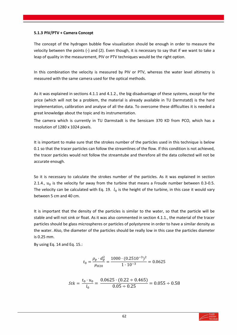
62
5.1.3 PIV/PTV + Camera Concept
The concept of the hydrogen bubble flow visualization should be enough in order to measure the
velocity between the points (-) and (2). Even though, it is necessary to say that if we want to take a
leap of quality in the measurement, PIV or PTV techniques would be the right option.
In this combination the velocity is measured by PIV or PTV, whereas the water level altimetry is
measured with the same camera used for the optical methods.
As it was explained in sections 4.1.1 and 4.1.2., the big disadvantage of these systems, except for the
price (which will not be a problem, the material is already available in TU Darmstatd) is the hard
implementation, calibration and analyse of all the data. To overcome these difficulties it is needed a
great knowledge about the topic and its instrumentation.
The camera which is currently in TU Darmstadt is the Sensicam 370 KD from PCO, which has a
resolution of 1280 x 1024 pixels.
It is important to make sure that the strokes number of the particles used in this technique is below
0.1 so that the tracer particles can follow the streamlines of the flow. If this condition is not achieved,
the tracer particles would not follow the streamtube and therefore all the data collected will not be
accurate enough.
So it is necessary to calculate the strokes number of the particles. As it was explained in section
2.1.4., 𝑢0 is the velocity far away from the turbine that means a Froude number between 0.3-0.5.
The velocity can be calculated with Eq. 19. 𝑙0 is the height of the turbine, in this case it would vary
between 5 cm and 40 cm.
It is important that the density of the particles is similar to the water, so that the particle will be
stable and will not sink or float. As it was also commented in section 4.1.1., the material of the tracer
particles should be glass microspheres or particles of polystyrene in order to have a similar density as
the water. Also, the diameter of the particles should be really low in this case the particles diameter
is 0.25 mm.
By using Eq. 14 and Eq. 15.:
𝑡0 =𝜌𝑝 · 𝑑𝑝
2
𝜇𝐻20=
1000 · (0.2510−3)2
1 · 10−3= 0.0625
𝑆𝑡𝑘 = 𝑡0 · 𝑢0
𝑙0=
0.0625 · (0.22 ÷ 0.465)
0.05 ÷ 0.25= 0.055 ÷ 0.58
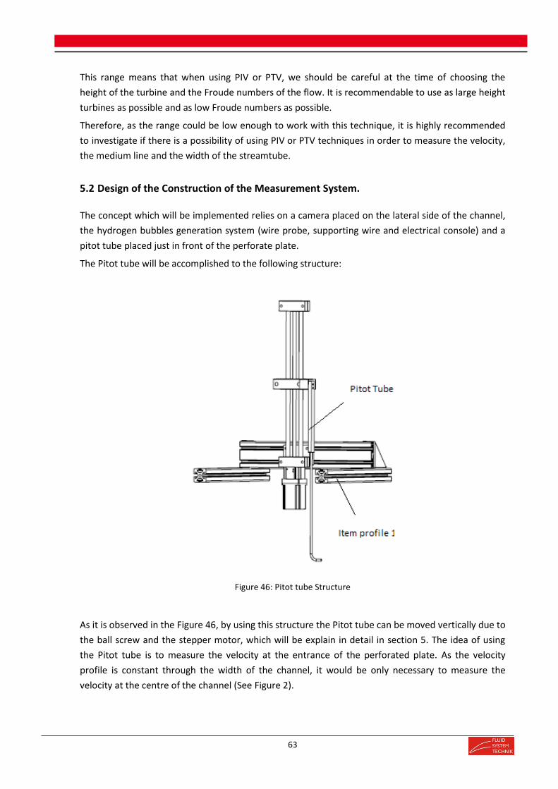
63
This range means that when using PIV or PTV, we should be careful at the time of choosing the
height of the turbine and the Froude numbers of the flow. It is recommendable to use as large height
turbines as possible and as low Froude numbers as possible.
Therefore, as the range could be low enough to work with this technique, it is highly recommended
to investigate if there is a possibility of using PIV or PTV techniques in order to measure the velocity,
the medium line and the width of the streamtube.
5.2 Design of the Construction of the Measurement System.
The concept which will be implemented relies on a camera placed on the lateral side of the channel,
the hydrogen bubbles generation system (wire probe, supporting wire and electrical console) and a
pitot tube placed just in front of the perforate plate.
The Pitot tube will be accomplished to the following structure:
Figure 46: Pitot tube Structure
As it is observed in the Figure 46, by using this structure the Pitot tube can be moved vertically due to
the ball screw and the stepper motor, which will be explain in detail in section 5. The idea of using
the Pitot tube is to measure the velocity at the entrance of the perforated plate. As the velocity
profile is constant through the width of the channel, it would be only necessary to measure the
velocity at the centre of the channel (See Figure 2).

64
It is also important to notice that the Pitot tube could also measure the velocity between the points
(1) and (+) by changing the position of the items profiles 1, by doing these changes it is possible to
get the whole distribution of the velocity between (1) and (+).
There are components which are not marked because they will be explained in detail in section 5.
The main function of these pieces resides in the Turbine Concept although they are also used in the
construction of the Pitot tube structure in order to profit the design of the pieces.
Note that the Pitot tube shown in Figure 46, is already set in the laboratory, the original technical
drawings were not available in the database of TU Darmstadt, so piece 12 is just an imitation of it.
As it has been previously commented the two vertical supporting wire probes will be fixed in the
profile item 1 as it is shown in the following assembly: Both wire probes will be installed at a distance
of 15 mm, each in one side of the Turbine support. The supporting wire probe will be then screwed
to the item profile 1, shown in Figure 46. It is important to note that the distances between the end
of the item profile 1 and the adaptor 1 must be kept, if not the wire probe will touch the wall of the
channel test rig. By using this structure, the supporting wire probe will be fixed always.
The technical drawings of the wire support and the adaptor 3 are attached in section 10. (Appendix
B).
Figure 47: Wire Probes Support
65
6 Turbine Concept
The requirements of the Turbine concept were settled in section 3. The turbine concept should
change automatically the perforated plate height position and should make easier the removable of
the turbine resistances and the perforated plate size (height) as it is explained in section 2.3.
There should be at least three different perforated plate resistances and each perforated plate
should have at least four different heights.
Also, the system should combine the Turbine structure with the Pitot tube structure in order to have
the technical drawings of the complete measurement system.
6.1 Election of the Turbine Concept
The Turbine Concept that is proposed in this thesis is composed of a Ball Screw from Igus, which
enables the turbine to move vertically in combination with the Stepper motor and the gear box
By using this concept it is quite easy to control the height position of the perforated plate by codding
in Labview and using a controller, which will be placed in out of the test rig. Programming the
Labview code is beyond this thesis but should be done by the person in charge of running the
measurement.
The combination of these components allows measuring the required parameters many different
points. Furthermore it allows collecting more data in less time in comparison with the current state
of the Turbine concept. Currently, the perforated plate’s height position can only be changed by
screwing the perforated plate in a different hole of the turbine support (see Figure 41.
With this concept, it will only be necessary to screw at the time of changing the perforated plate to
another one with different size. So the correct process of our measurement will be to collect all the
data of a single perforated plate size in different height positions and different turbine resistances
and then change the perforated plate size.
Currently it is necessary to screw every time that is necessary to change the height position, the
resistances and the perforated plate size.
Another advantage of this structure is that when changing the perforated plate size, it is possible to
position the turbine in the maximum height and screw in a more comfortable way. Nowadays it is
really uncomfortable because as it is shown in Figure 18, the turbine is fixed inside the test rig.
The turbine support will be longer than before, so that if it is necessary to change the size of the
perforated plate, it would be possible to screw outside of the test rig on the condition that the
turbine is positioned in the maximum height.

66
Figure 48: Lateral Turbine Concept
The technical drawing of the Adaptor L, Adaptor 1 and the colour version of Figure 48 are attached in
section 10 (Appendix B).
All the pieces which are attached in the Appendix B are pieces that do not exist currently and should
be fabricated in TU Darmstadt. The rest of pieces do not have technical drawings because they
already exist and are placed in the channel test rig. The majority of them were bought from Igus and
Rose&Krieger.
The item profiles shown in Figure 48 are from Rose&Krieger, the main function of them is to position
the structure in the centre of the test rig, they are not relevant to the functioning of the system.

67
It is important to talk about the force sensor (See section 2.2.).
In Figure 51, there are two red lines, which cannot be exceeded by any piece. This fact is really
important because if any piece touches the zone between both red lines the force sensor does not
work properly. Therefore, the turbine support and the Adaptor L must be design in a way that never
touch this area. This sensor will be the component in charge of measuring the force, which the flow is
producing in the perforated plate. As it has been previously commented, the sensor works greatly
with a measurement uncertainty of 0.1%
Figure 49: Force Sensor
Adaptor L is used to fix the turbine system to the ball screw, it must be deep enough so that the
turbine support does not touch the stepper motor, its shape places the turbine structure frontally,
but the ball screw is fixed laterally. Adaptor 1 is used to fix the ball screw to the item profiles, which
are fixed to the rest of the test rig, it must also be deep enough in order to avoid collision between
item profile 3 and the stepper motor.
One of the advantages of this concept is that by placing the ball screw laterally, we avoid the
structure bending when high velocities are used in the test rig. This fact is produced because the
surface which is normal to the flow is smaller than the transversal surface. This gives more rigidity to
the structure.

68
Although the lateral option is efficient, as it is placed in the lateral side of the test rig, it appears a
momentum, which is not desirable. To confront this con, it was decided to design the structure with
the minimum distance between the turbine structure and the ball screw: 5 cm. That means that the
momentum will not be that powerful to interfere in the measurement accuracy. The velocities that
we are working with are not going to be higher than 1.3 m/s.
There is another option which could also be test, a frontal structure with almost the same
components. It will move also vertically by using a ball screw a stepper motor, gearbox and a
controller which will be placed outside the test rig. The vertical movement will be programmed by
Labview.
The following picture shows the frontal concept
Figure 50: Frontal Turbine Concept
The only two differences with the lateral structure are the use of Adaptor 2 instead of Adaptor L and
the fact that the ball screw will be fixed to item profile 2 without using item profile 3 (See Figure 50).

69
The coloured version of Figure 50 is attached in section 10 (Appendix B).
In this option it does not appear a momentum because the turbine is fixed to an item profile
positioned normal to the flow. The main problem of this concept is that if the flow has high
velocities, the force produced may be too high and therefore the whole frontal structure could bend,
producing undesirable errors in the measurement parameters, because the turbine will change the
position and then the hydrogen bubbles will also change the path of the streamtube.
Although the Lateral option is the concept chosen, both, frontal and lateral structures have almost
the same pieces, this have been done so that both can be tested and therefore observe in the
experimentation which one works better.
6.2 Election Turbine Resistances
Turbine Resistances are defined as the shape of the perforated plate. It is directly related with the
dissipated energy of the turbine. There are plenty of different possibilities when choosing the shape
of the perforated plate, for instance square holes, round holes, vertical lines, etc.
The dissipated energy is of high importance in this experiment. As it was commented in section 2.1.,
it does not matter what kind of energy is dissipated, but what really matters is the amount of the
dissipated energy. For this experiment is necessary to achieve a wide range of dissipated energy.
In this case a high upper limit of the range is easy to achieve, so we should focus on the lower limit,
and try to make it as low as possible. In order to achieve this purpose, ξ is defined as the resistance
coefficient, which is the force caused by an obstacle placed against a water flow. It is usually
expressed in kg/m2. [40]
The lower the resistance coefficient is, the lower the perforated plate dissipates energy.
In Eq. 32 is defined the resistance coefficient. [40]
With the conditions that 𝑅𝑒 > 105 just after the turbine and that the coefficient 𝑙
𝐷ℎ= 0 ÷ 0.015
In our case 𝑅𝑒𝑚𝑎𝑥 = 2.4 · 105 and 𝑙
𝐷ℎ=
2
320= 0.00625

70
Figure 51: Sketch of turbine resistance [40]
𝜉 = (0.707√1 − 𝜑 + 1 − 𝜑)2 ·1
𝜑2 (Eq. 32)
This coefficient depends on the cross-section coefficient 𝑓,̅ the Reynolds number and the shape of its
orifices.
The cross-section coefficient is defined in the following equation.
φ = 𝐴𝑜𝑝𝑒𝑛
𝐴𝑐𝑙𝑜𝑠𝑒
(Eq. 33)
Figure 52: Values of the resistance coefficient in function of the cross-section coefficient [40]

71
As it has been explained, the objective is to analyse the measurement with low energy dissipation,
this is achieved with a low resistance coefficient. By increasing the cross-section coefficient, it is
achieved a diminution of the resistance coefficient.
The only solution then is to make bigger the open area, it is recommend to use square holes instead
of round holes in the perforated plate, with this orifices shape, the perforated plate dissipates lower
energy which was the objective.
There will be six different perforated plate sizes, the width will be always 200 mm but the height will
be of 50 mm, 100 mm, 150mm, 200mm, 250 mm (which is 𝐻1) and one perforated plate size, which
blocks the whole channel of 400 mm.
The holes sizes that are proposed are:
5 mm square hole with a separation between the centres of 8 mm (1000x2000)
8 mm square hole with a separation between the centres of 12 mm (1000x2000)
10 mm square hole with a separation between the centres of 15 mm (1000x2000)
The material will be steel due to its low price. The perforated plates can be bought in Shopmetal.de.
Figure 53: Square perforated plates (Turbine resistances)

72

73
7 Summary and Outlooks
7.1 Summary
In light of the above mentioned, it is important to make some conclusions of the present bachelor
thesis.
The elected Measurement system can be divided in velocity measurement and water level altimetry
measurement.
The velocity will be measured with a Flow visualization technique, more concretely with the
hydrogen bubble method, the electric circuit used in order to generate the bubbles by electrolysis is
the one shown in Figure 42, the wire will be of platinum and the wires support od brass with an
insulation of shrink-fit, the illumination will consist of one LED in the bottom of the channel and
other two oblique to the area of interest. By using this technique, it will be possible to measure the
distribution of the velocity between points (-) and (2) as well as the medium line and the width of the
streamtube.
A Pitot tube will be used to measure the velocity before the perforated plate. Also, the foils concept
explained previously will be used just to show the flow’s behaviour to other people or institutions.
The water level altimetry will be measured with the same high-resolution camera used in the velocity
measurement. At TU Darmstadt there is already a Charge Coupled Device (CCD) Camera: Sensicam
qe. By making a lot of pictures and interpolating it will not be difficult to measure the shape of the
water flow altimetry. By using this technique, it would be possible to measure the water level
altimetry as well as the static pressure, which depends directly on the height.
The turbine system, which has been designed in the present thesis consist of a ball screw, a stepper
motor, a gearbox and a controller. The vertical movement of this system will be coded in Labview.
This concept allows measuring the required parameters in different height positions without
screwing in the turbine support. Also, it will not be necessary to screw when changing the perforated
plate resistances. The only moment that will be necessary to screw is when changing the size of the
perforated plate.
By implementing the proposed turbine system, it is gained velocity at the time of collecting data and
comfortability when changing the resistances or sizes of the perforated plates.
The turbine system will have a lateral structure (Figure 48) in order to avoid a bending force
produced by the water flow, the distance between the ball screw and the turbine support will be
minimal in order to avoid an undesirable momentum.

74
As the pieces used in the construction of the lateral structure are almost the same as the ones that
could be used to construct a frontal structure (Figure 50) it could be interesting to test both
experimentally and then choose the most efficient structure. Even though, the frontal structure
could present bending forces and could change the position of the turbine, resulting in inaccurate
measurements.
7.2 Outlooks
Although the hydrogen bubble technique should work efficiently, if it is wanted a leap of quality in
the project it would be recommendable to use PIV or PTV techniques, which are way more accurate
than the hydrogen bubble method. The material is available in TU Darmstadt. The main disadvantage
of these techniques is the hard implementation.
In this case the water level altimetry measurement will consist of the same camera used for the
optical method. It is the same concept that the one present in this thesis.
If the future path does not follow immediately the PIV or PTV techniques, it would be a good idea to
invest in a laser sheet in order to illuminate the area of interest where the camera will focus on the
hydrogen bubbles. This laser sheet will be also necessary in the PIV or PTV techniques, so it would be
nice to start with this step.
The person responsible of running the measurement should consider that is necessary the calibration
of the signal TTL by calibrating the components 𝑅1 and 𝐶1 as well as the angle of LEDs position.
In the turbine system, it is also necessary to program the code of Labview to move vertically the Pitot
tube and the perforated plate.

75
8 References
[1] Renewables 2017 Global Status Report - Ren21, 2017.
[2] Lombardo, Crystal. The Advantages and Disadvantages of Tidal Energy Power - The Next
Galaxy, 2015.
[3] Hermes, Jennifer. The present and Future of Tidal Power - Environmental leader, 2013.
[4] Pelz, P.F. Upper Limit for Hydropower in an Open-Chanel Flow. J. Hydraul. Eng., 137(11),
1536-1542. American Society of Civil Engineers. 2011.
[5] Pelz, P.F; Metzler M. An Analytic Approach to Optimization of Tidal Turbine Fields. ICEPE
2013 - 3rd International Conference on Energy Process Engineering. Frankfurt, Deutschland.
2013.
[6] J. Nieschlag. Experimentelle Untersuchung der Strömung um eine vertikal umströmte
hydrokinetische Turbine, Darmstadt 2016
[7] D. Hernández Días. Design and Construction of an Open Channel Test Rig. Bachelor-Thesis.
Darmstadt. 2013.
[8] Lehr, M. Aufbau eines Messsystems zur Strömungsvermessung am offenen
Gerinneprüfstand. Master-Thesis. Darmstadt. 2014.
[9] M. Euler, A. Krah, M. Lehr, X. Li. Design eines Messsystems für einen Gerinneprüfstand.
Advanced Design Project. Darmstadt. 2013.
[10] Deparment FST ( Fluid System Technik) - TU Darmstadt.
[11] Çengel, Yunus A; Cimbala, John M. Fluid Mechanics [Fundamentals and Applications] 1st
Edition in SI Units. New York Mc.Graw-Hills 2006.
[12] Shames, I.H. Mechanics of Fluids. New York McGraw-Hill Higher Education, 2004.
[13] Mott, Robert L.. Applied Fluid Mechanics. 6th Edition. New Jersey: Pearson Prentice Hall.
2006.
[14] Cameron Tropea; Alexander Yarin; John Foss (eds.). Springer Handbook of Experimental Fluid
Mechanics. Springer.
[15] Starke, Oliver. Konstruktion eines Prüfstandes zur experimentellen Validierung von
Gezeitenturbinenmodellen. Darmstadt 2017
[16] Froehlich, T. Performance survey of an open channel test rig. Master-Thesis. Darmstadt.
2015.
[17] Dr. R.B. Green. An introductory course for advanced experimental techniques used in fluid
dynamics and aerodynamics. United Kingdom: University of Glasgow. 2009.
[18] Ronald J, Adrian. Particle-Imaging Techniques for Experimental Fluid Mechanics. University of
Illinois. 1991.
[19] W. Nitsche, A. Brunn. Strömungsmesstechnik. Springer-Verlag. Berlin, Heidelberg. 2006.

76
[20] http://www.andor.com/learning-academy/piv-mode-for-istar-scmos-technical-article
[21] TH. Dracos. Three-Dimensional Velocity and Vorticity Measuring and Image Analysis
Techniques, Zürich 1996.
[22] K. Rubner, D. Bohn. Verfahren für die Auswertung der Messergebnisse von Strömungs
sonden durch mehrdimensionale Approximation der Eichkurven und Eichflächen. Zeit-schrift
für Flugwissenschaften 20. 1972.
[23] http://ocw.metu.edu.tr/pluginfile.php/1871/mod_resource/content/0/AE547/AE47_9_Hotw
ire-son.pdf (20/08/2013)
[24] Dantec Dynamics. Probes for Hot-wire anemometry. Product Catalog.
[25] R. Markert. Strukturdynamik. Vorlesungsskript. Fachgebiet Strukturdynamik. Darmstadt.
2010.
[26] Durst, F.A. Melling; J.Whitelaw. Principles and Practices of Laser Doppler Anemometry.
Academic Press. 1981.
[27] Dantec Dynamics. Measurement Principles of Laser Dopler Anemometry.
[28] Manoochehr M. Koochesfahani and Daniel G. Nocera. Molecular Tagging Velocimetry.
Handbook of Experimental Fluid Dynamics, Chapter 5.4, editors: J. Foss, C. Tropea and A.
Yarin, Springer-Verlag . 2007).
[29] C. R. Smith and R. D. Paxson. A Technique for Evaluation of Three-dimensional Behavior in
Turbulent Boundary Layers Using Computer Augmented Hydrogen Bubble-wire Flow
Visualization. Bethlehem. 1983.
[30] W. Merzkirch. Techniques of Flow Visualization, AGARD, editor: K.Gersten. Essen 1987.
[31] Taif M. Mansoor, Prof. Dr. Akram W. Ezzat. Water Flow Visualization And Velocity
Measurement Using Hydrogen Bubble Generation Technique In Low Speed Open Channel.
Baghdad 2012.
[32] Flow Visualization: Techniques and Examples, Edition: Second, Publisher: Imperial College
Press, London, Editors: A. J. Smits, T.T. Lim, pp.19
[33] Mattingly, George E. The Hydrogen-Bubble, Flow Visualization Technique. Washington, D.C.
:Dept. of the Navy, David Taylor Model Basin,1966.
[34] R. Budwig, R. Peattie. Two new Circuits for Hydrogen Bubble Flow Visualization. Moscow
1988.
[35] L.J.Lu, C.R.Smith Image processing of Hydrogen Bubble Flow Visualization for Determination
of Turbulence Statistics and Bursting Characteristics. Bethlehem 1985.
[36] C.Magness, T. Utsch, D.Rockwell. Flow Visualization via Laser-Induced Reflection from Bubble
Sheets. Bethlehem 1990.
[37] M. Löffler-Mang. Optische Sensorik. Springer-Verlag. Berlin, Heidelberg. 2012.
[38] Hopper, Henry. A Dozen Ways to Measure Fluid Level and How they work. Sensors|Online.
2004.
[39] Recommended Light Levels (Illuminance) for Outdoor and Indoor Venues

77
[40] Idel’chik. Handbook of Hydraulic Resistance [Coefficients of Local Resistance and of Friction].
Jerusalem: Israel Program for Scientific Translations. 1966.
9 Appendix A
9.1 List of Figures
Figure 1: Final Energy Consumption 2015 [1] .......................................................... 7
Figure 2 Flow Simulation of the Experiment [10]. .............................................. 9
Figure 3: Control Volume with variant cross-section [7] ........................... 11
Figure 4: Volume and Surfaces Forces. [7] ............................................................. 12
Figure 5: Flows state depending on Re and Fr ..................................................... 15
Figure 6: Overview of the occurrence of various surface phenomena
[6] ................................................................................................................................... 15
Figure 7: Small Gravity Wave [6] .................................................................................. 16
Figure 8: Large Gravity Wave [6] .................................................................................. 16
Figure 9: Hydraulic Jump [6] ............................................................................................ 16
Figure 10: Stokes Number Behaviour of the Flow ................................................. 17
Figure 11: Specific energy with Fluid depth ........................................................ 18
Figure 12: Test rig 3D [10]. ............................................................................................ 19
Figure 13: Test rig 2D [10] .............................................................................................. 20
Figure 14: Velocity Map in the channel for Fr=1.4 [6] ................................ 22
Figure 15: Modular Concept in an Open Channel ................................................... 22
Figure 16: Bending Beam Load Sensor [8] ................................................................. 23
Figure 17: Test results of the Conductive Level Altimetry technique24
Figure 18: Channel test rig, side view. ................................................................. 25
Figure 19: PIV Functioning [20] ..................................................................................... 32
Figure 20: PIV 3D ...................................................................................................................... 33
Figure 21: Pitot Tube ............................................................................................................ 35
Figure 22: Multi Hole Probe [8] ..................................................................................... 36
Figure 23: Measurement principles of CTA [23] ................................................... 37
Figure 24: Circuit of a hot wire probe [24] ........................................................ 37
Figure 25: Operation principle of a hot wire probe [22] ........................... 38
Figure 26: Different Types of Hot Wire Probes [23] ....................................... 38
Figure 27: Functioning of Laser Doppler Anemometry [27] ........................... 39

78
Figure 28: Funcitoning of MTV ......................................................................................... 40
Figure 29: Flow visualization with foils. ............................................................. 41
Figure 30: Hydrogen Bubble................................................................................................. 42
Figure 31: Types of wire probes [32] ......................................................................... 44
Figure 32: High Power LED ................................................................................................... 45
Figure 33: Laser Light Sheets ......................................................................................... 45
Figure 34: CCD Camera (Sensicam qe) ........................................................................... 47
Figure 35: Functioning of the Laser Distance Sensor [29] ......................... 48
Figure 36: Scheme of the Conductive Level Altimetry method [8] .......... 49
Figure 37: Description of Capacitive Level Altimetry method [29] ...... 49
Figure 38: Ultrasonic Measurement [38] .................................................................... 50
Figure 39: Radar Level Altimetry measurement ..................................................... 51
Figure 40: Magnetostrictive Level Transmitters ................................................. 52
Figure 41: Turbine Structure ................................................................................................. 54
Figure 42: Electric Circuit for Hydrogen Bubble Generation. [34] ...... 56
Figure 43: Polarity switch for cleaning ................................................................. 58
Figure 44: Flow Visualization ......................................................................................... 59
Figure 45: Vertical Wire ..................................................................................................... 60
Figure 46: Pitot tube Structure ..................................................................................... 63
Figure 47: Wire Probes Support ....................................................................................... 64
Figure 48: Lateral Turbine Concept ............................................................................. 66
Figure 49: Force Sensor ........................................................................................................ 67
Figure 50: Frontal Turbine Concept ............................................................................. 68
Figure 51: Sketch of turbine resistance [40] ..................................................... 70
Figure 52: Values of the resistance coefficient in function of the
cross-section coefficient [40] .................................................................. 70
Figure 53: Square perforated plates (Turbine resistances) ...................... 71
9.2 List of Tables
Table 1: Functional Specific Document ................................................................................ 28
Table 2: Evaluation of Velocity Measurement Techniques ................................................... 31
Table 3: Evaluation of the Water level Measurement techniques ......................................... 46

79
9.3 Economic Budget
In this Section, it will be explained all the costs which have been surrounded in this thesis. It is
considered that the student would have a salary of 12 €/ hour. It is also considered that the student
has work in the thesis around 375 hours.
So, the human cost of the present bachelor thesis would be of 4.500 €
In the following table, it is shown all the required components which must be bought by TU
Darmstadt in order to make possible the realization of this thesis. As it can be observed the material
cost is 539.79 €
Component Company Nº of Reference Price
Isolated Transformer x2 Digikey N-73A (Triad Magnets) 73.02 euros
Rectifier x2 Mouser MDA206G 1.12 euros
Opto-isolator x2 Mouser 859-4N26 0.84 euros
Multivibrator Monostable x2 Digikey SN74121D 6.76 euros
Transistor MOSFET x2 Octopart MTP4N50 20.42 euros
Capacitor 500 μF and 450 V x2
Mouser E36D451LPN500TA54M 18.76 euros
Resistor 0.3 kΩ x2 Digikey RC04022JR-07300RL 0.16 euros
Resistor 20 kΩ x2 Digikey RC0201FR-0720KL 0.16 euros
Resistor 0.1 kΩ (10W) x2 Digikey RC0603FR-07100RL 0.16 euros
Resistor 20 kΩ (2W) x2 Digikey 352120KFT 1.14 euros
Circuit breaker 2 A x2 Digikey 9926251902 38.74 euros
Wire Platinum Buyplatinumwire.com 50 μm x 3,048 m 99.52 euros
Brass round bar Metalandplastic 4mm x 3 m 8.83 euros
LED of 1120 lumens Mouser XHPTOB-00-0000-000BJ450E 5.75 euros
LED of 400 lumens x 2 Mouser XPLAWT-00-0000-000BV20E3 5.38 euros
Perforated Sheet 5mm Shopmetal Lochblech aus Stahl roh DC/DD/S235 - QG 5-8 2x1000x2000
98.28 euros
Perforated Sheet 8mm Shopmetal Lochblech aus Stahl roh DC/DD/S235 - QG 8-12 2x1000x2000
78.47 euros
Perforated Sheet 10mm Shopmetal Lochblech aus Stahl roh DC/DD/S235 - QG 10-15 2x1000x2000
82.28 euros
Total 539.79 euros

80
In the following table, it is shown all the costs which have been involved in the realization of this project:
Resource Cost (€)
Human Cost 4.500
Material Cost 539,79
General Cost 503,98
Industry Surcharge 453,58
IVA (21%) 1259,4435
Total 7.257
Consequently, the Total Costs of the project are estimated in 7.257 €
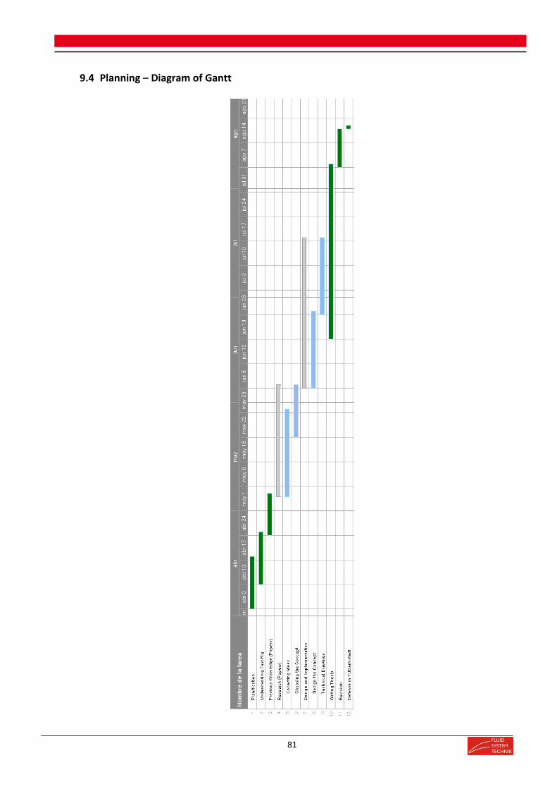
81
9.4 Planning – Diagram of Gantt

82

83
10 Appendix B – Technical Drawings

84

85
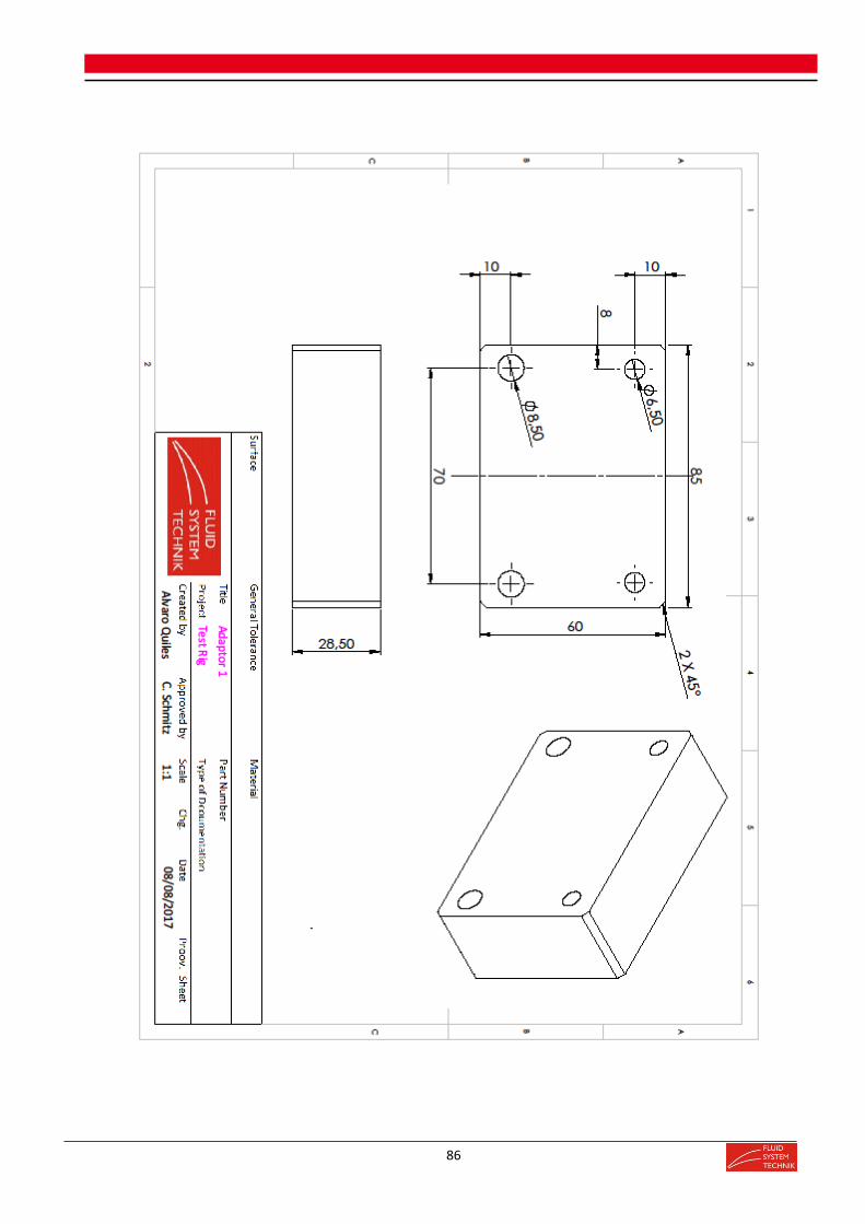
86

87
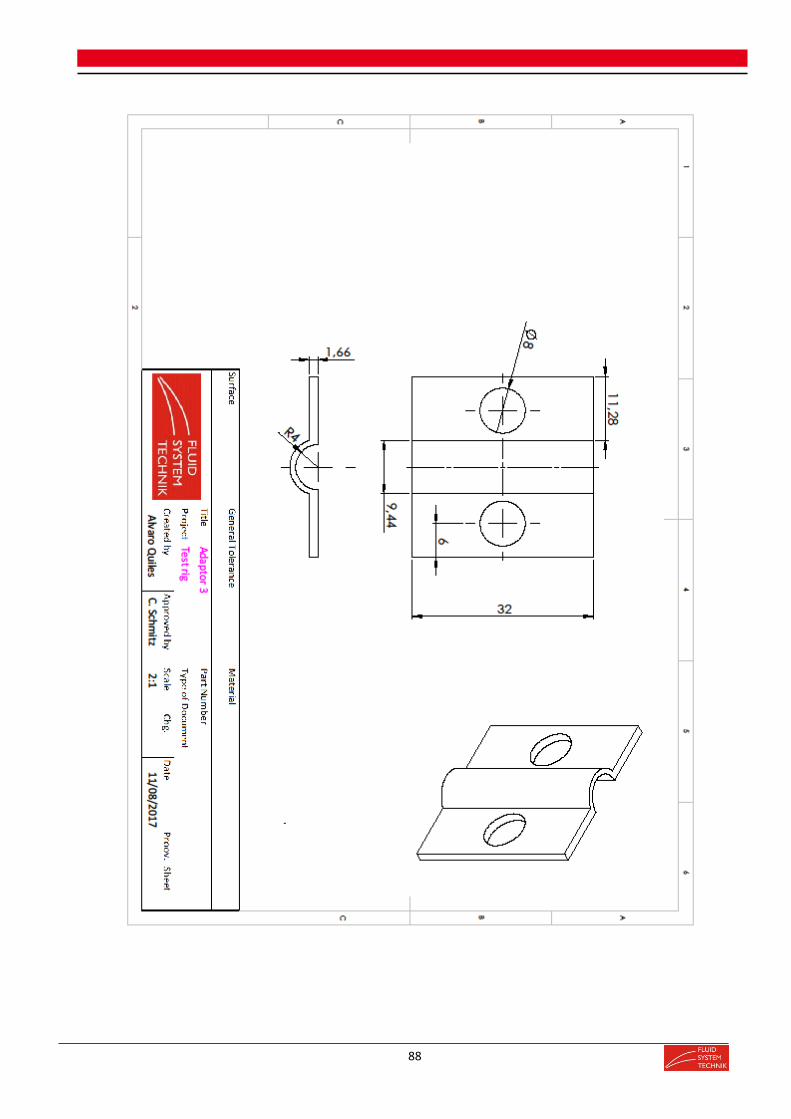
88

89

90

91
Figure: Frontal Turbine Concept

92
Figure: Lateral Turbine Concept.