Hiperciclicidad en espacios de funciones holomorfas y...

UNIVERSIDAD DE BUENOS AIRES

Facultad de Ciencias Exactas y Naturales

Departamento de Matematica

Hiperciclicidad en espacios de funciones holomorfas y pseudo orbitas deoperadores lineales.

Tesis presentada para optar al tıtulo de Doctor de la Universidad de Buenos Aires en el area

Ciencias Matematicas

Martın Savransky

Director de tesis: Dr. Damian Pinasco.

Director Asistente: Dr. Santiago Muro.

Consejero de estudios: Dr. Daniel Carando.

Buenos Aires, 5 de octubre de 2015

Fecha de defensa: 14 de diciembre de 2015

Hiperciclicidad en espacios de funciones holomorfas y pseudoorbitas de operadores lineales

Resumen

En esta tesis estudiamos distintos problemas sobre densidad de orbitas de operadores lineales.

Un operador lineal se dice hipercıclico si admite una orbita densa. Podemos decir que el centro

de atencion es el comportamiento de las sucesivas iteraciones de un operador lineal. En otras

palabras, se estudian sistemas dinamicos discretos asociados a operadores lineales. En el contexto

finito dimensional este problema se puede resolver a traves del estudio de la forma de Jordan

asociada a una matriz, y los comportamientos son relativamente simples (de ahı que el caos se

asocia naturalmente a sistemas no lineales). Sin embargo, en espacios de dimension infinita los

sistemas lineales pueden ser caoticos, ya que aparecen fenomenos nuevos, como por ejemplo la

existencia de orbitas densas en todo el espacio.

Los primeros ejemplos de operadores hipercıclicos surgieron en el contexto de la teorıa de

funciones analıticas. Ası, en 1929, G. D. Birkhoff [Bir29] probo que para todo a ∈ C, a 6= 0,

el operador traslacion en el espacio de funciones enteras de variable compleja (H(C), τ) con la

topologıa compacto-abierta, Ta : H(C)→ H(C) definido por Taf(z) = f(z+a) es hipercıclico, y

en 1952, G. R. MacLane [Mac52], demostro que lo mismo ocurre con el operador de diferenciacion

en H(C). Estos resultados fueron generalizados por G. Godefroy y J. H. Shapiro en 1991 [GS91]

quienes probaron que todo operador lineal y continuo T : H(C) → H(C) que conmute con las

traslaciones y no sea un multiplo de la identidad es hipercıclico. Esta familia de operadores

se conoce por el nombre de operadores de convolucion. En esta tesis estudiamos operadores

de convolucion definidos en espacios de funciones holomorfas sobre espacios de Banach. Ası

como tambien damos ejemplos de operadores fuera de la clase de la familia de los operadores de

convolucion que resultan hipercıclicos. Estos ejemplos se presentan tanto en espacios de funciones

holomorfas de finitas variables complejas y tambien en espacios de funciones holomorfas definidas

en espacios de Banach de dimension infinita.

Por otro lado, estudiamos pseudo orbitas de opeadores lineales. Decimos que {xn}n∈N es

una (εn)−pseudo orbita para T si d(xn+1, T (xn)) ≤ εn para todo n ∈ N. Esta definicion cobra

sentido cuando se permite cometer un error en cada paso de la iteracion del sistema. Notemos

que si εn = 0 para todo n ∈ N, una (εn)-pseudo orbita es una orbita. Decimos que el operador T

es (εn)-hipercıclico si existe una pseudo orbita densa para la sucesion de errores (εn). Estudiamos

este concepto enmarcado dentro de la teorıa de sistemas dinamicos lineales.

Palabras clave: Operadores Hipercıclicos, Pseudo Orbitas, Operadores de Convolucion, Funciones Holo-

morfas.

3

Hypercyclicity in spaces of holomorphic functions and pseudoorbits of linear operators

Abstract

In this thesis we study several problems on the density of orbits of linear operators. A linear

operator is said hypercyclic if admits a dense orbit. We can say that the spotlight is the behavior

of successive iterations of a linear operator. In other words, dynamical systems associated to

linear operators are studied. In the finite dimensional context the problem is relatively simple

and it can be solved through the canonical Jordan form of a matrix. Hence, chaos is usually

associated to non linear systems. However, in infinite dimensional spaces linear operators can

be chaotic since new phenomena appears, such as the existence of dense orbits.

The first examples of hypercyclic operators came out in the context of analytic functions.

Birkhoff in [Bir29] proved that for every a ∈ C, a 6= 0, the translation operator on the space

of one complex variable functions (H(C), τ) with the compact-open topology, τa : H(C) →H(C) defined by τaf(z) = f(z + a) is hypercyclic. MacLane in [Mac52], proved that the same

occurs with the derivative operator on the space H(C). Both results were generalized by a

remarkable theorem due to Godefroy and Shapiro [GS91], who proved that every linear operator

that commutes with the translation on H(CN ) and is not a scalar multiple of the identity

is hypercyclic. This family of operators is known as the class of (non trivial) “convolution

operators”. In this thesis we study convolution operators defined on spaces of holomorphic

functions on Banach spaces. In addition, we show examples of non convolution hypercyclic

operators defined on spaces of holomorphic functions of finite complex variables and also for

spaces of holomorphic functions defined on infinite dimensional Banach spaces.

On other side, we deal with pseudo orbits of linear operators. We say that {xn}n∈N is

a (εn)−pseudo orbit of T if d(xn+1, T (xn)) ≤ εn for any n ∈ N. This definition becomes

meaningful when a small measurement error is committed in each step of the iteration. We

say that an operator T is (εn)-hypercyclic if admits a dense pseudo orbit for the error sequence

(εn)n∈N. We study this new concept framed on the theory of linear dynamical systems.

Keywords: Hypercyclic operators, Pseudo orbits, Convolution Operators, Holomorphic Functions.

5

Contents

Introduccion 1

Introduction 5

1 Linear Dynamics 9

1.1 Hypercyclic operators . . . . . . . . . . . . . . . . . . . . . . . . . . . . . . . . . 9

1.2 Spectral properties . . . . . . . . . . . . . . . . . . . . . . . . . . . . . . . . . . . 12

1.3 Other notions in linear dynamics . . . . . . . . . . . . . . . . . . . . . . . . . . . 13

2 Chain Transitive Operators 17

2.1 (εn)-hypercyclic operators . . . . . . . . . . . . . . . . . . . . . . . . . . . . . . . 18

2.2 Some non trivial examples . . . . . . . . . . . . . . . . . . . . . . . . . . . . . . . 24

2.3 The spectrum of a (εn)-hypercyclic operator . . . . . . . . . . . . . . . . . . . . . 33

2.4 Criteria for (εn)-hypercyclicity . . . . . . . . . . . . . . . . . . . . . . . . . . . . 35

2.5 Weighted shifts . . . . . . . . . . . . . . . . . . . . . . . . . . . . . . . . . . . . . 39

2.5.1 Unilateral weighted shifts . . . . . . . . . . . . . . . . . . . . . . . . . . . 39

2.5.2 Bilateral weighted shifts . . . . . . . . . . . . . . . . . . . . . . . . . . . . 42

3 Hypercyclic behavior of some non-convolution operators 45

3.1 Non-convolution operators on H(C) . . . . . . . . . . . . . . . . . . . . . . . . . 46

3.2 Non-convolution operators on H(CN ) . . . . . . . . . . . . . . . . . . . . . . . . 48

3.2.1 The diagonal case . . . . . . . . . . . . . . . . . . . . . . . . . . . . . . . 48

3.2.2 The non-diagonal case . . . . . . . . . . . . . . . . . . . . . . . . . . . . . 56

4 Holomorphic functions on Banach spaces 63

4.1 Holomorphic functions of A-bounded type . . . . . . . . . . . . . . . . . . . . . . 63

5 Strongly mixing convolution operators on Frechet spaces 67

5.1 Strongly mixing convolution operators . . . . . . . . . . . . . . . . . . . . . . . . 68

5.2 Exponential growth conditions for frequently hypercyclic entire functions . . . . 70

5.3 Frequently hypercyclic subspaces and examples . . . . . . . . . . . . . . . . . . . 73

5.3.1 Frequently hypercyclic subspaces . . . . . . . . . . . . . . . . . . . . . . . 73

5.3.2 Translation operators. . . . . . . . . . . . . . . . . . . . . . . . . . . . . . 75

5.3.3 Differentiation operators. . . . . . . . . . . . . . . . . . . . . . . . . . . . 77

6 Non-convolution hypercyclic operators 79

6.1 Non-convolution operators in HbA(E) . . . . . . . . . . . . . . . . . . . . . . . . . 79

6.2 Hypercyclic behavior of the operator . . . . . . . . . . . . . . . . . . . . . . . . . 84

6.2.1 Holomorphic functions of compact bounded type . . . . . . . . . . . . . . 94

Bibliography 97

Contents

2

Introduccion

El estudio de la dinamica de operadores lineales definidos en espacios de Banach o de Frechet es

una rama moderna del analisis funcional que ha surgido a partir del trabajo de muchos autores.

Probablemente, el inicio de su estudio de manera sistematica es la tesis doctoral de C. Kitai en

1982 [Kit82]. En particular, gran parte de la difusion de este tema de estudio debe ser atribuida

a los trabajos de G. Godefroy y J. H. Shapiro [GS91] y K.-G. Grosse-Erdmann [GE99].

Para dar una idea sumamente simplificada del tema, podemos decir que el centro de atencion

es el comportamiento de las sucesivas iteraciones de un operador lineal. En otras palabras, se

estudian sistemas dinamicos discretos asociados a operadores lineales. En el contexto finito

dimensional este problema se puede resolver a traves del estudio de la forma de Jordan asociada

a una matriz, y los comportamientos son relativamente simples (de ahı que el caos se asocia

naturalmente a sistemas no lineales). Sin embargo, en espacios de dimension infinita los sistemas

lineales pueden ser caoticos, ya que aparecen fenomenos nuevos, como por ejemplo la existencia

de orbitas densas en todo el espacio. La palabra “hipercıclico” tiene su origen en la nocion de

“operador cıclico”, ligado al problema del subespacio invariante. En este caso, los operadores

hipercıclicos estan ligados al problema de existencia de subconjuntos invariantes: ¿dado un

operador lineal T : X → X, es posible encontrar un subconjunto cerrado no trivial F tal que

T (F ) ⊂ F?

Sea X un espacio de Frechet separable de dimension infinita y T : X → X un operador lineal

y continuo. Dado x ∈ X, la orbita de x por T es el conjunto definido por

Orb(x, T ) = {Tnx : n ≥ 0}.

El operador T se dice hipercıclico si existe x ∈ X (vector hipercıclico) tal que Orb(x, T ) es densa

en X.

Es importante notar que la existencia de operadores con esta propiedad es solo posible en

espacios de dimension infinita ya que por ejemplo, si T : X → X es un operador lineal en un

espacio de Frechet y T ′ : X ′ → X ′ es su operador adjunto, la existencia de algun autovalor para

T ′ garantiza que T no es hipercıclico. En los ultimos anos el estudio de la hiperciclicidad de

operadores ha tenido un desarrollo importante, como referencia puede consultarse la bibliografıa

[BM09] y [GEPM11].

Los primeros ejemplos de operadores hipercıclicos surgieron en el contexto de la teorıa de

funciones analıticas. Ası, en 1929, G. D. Birkhoff [Bir29] probo que para todo a ∈ C no nulo,

el operador traslacion en el espacio de funciones enteras de variable compleja (H(C), τ) con la

topologıa compacto-abierta, Ta : H(C)→ H(C) definido por Taf(z) = f(z+a) es hipercıclico, y

en 1952, G. R. MacLane [Mac52], demostro que lo mismo ocurre con el operador de diferenciacion

1

Introduccion

en H(C). Por supuesto, no existıa aun la nocion de hiperciclicidad, y el interes de estos trabajos

no se centraba en la dinamica de los operadores sino en propiedades de las funciones analıticas.

Estos resultados fueron generalizados por G. Godefroy y J. H. Shapiro en 1991 [GS91] quienes

probaron que todo operador lineal y continuo T : H(C)→ H(C) que conmute con las traslaciones

y no sea un multiplo de la identidad es hipercıclico. Estos operadores se denominan operadores

de convolucion no triviales. Versiones similares de este resultado para espacios de Frechet de

funciones analıticas definidas en un espacio de Banach fueron obtenidas en [CDM07, Pet01,

Pet06, AB99, BBFJ13].

El primer ejemplo de existencia de esta clase de operadores en espacios de Banach fue

exhibido por S. Rolewicz en 1969 [Rol69]. En su trabajo prueba que para 1 ≤ p < ∞, si

S : `p → `p es el operador shift a izquierda, S(x1, x2, x3, . . .) = (x2, x3, . . .), entonces T = λS

es hipercıclico para todo λ ∈ C, |λ| > 1. Tambien se plantea el problema de determinar si en

todo espacio de Banach separable de dimension infinita existen operadores hipercıclicos. Una

respuesta positiva a esta pregunta fue dada independientemente por S. I. Ansari [Ans97] y

L. Bernal [BG99] en 1997 y 1999 respectivamente. En el contexto de espacios de Frechet, la

existencia de operadores hipercıclicos fue probada por J. Bonet y A. Peris [BP98].

Un operador es hipercıclico en X si y solo si es topologicamente transitivo sobre abiertos,

es decir, para cada par de abiertos no vacıos U, V ⊂ X existe n ∈ N tal que Tn(U) ∩ V 6= ∅.En 2004, F. Bayart y S. Grivaux [BG04] generalizan esta definicion imponiendo condiciones a la

frecuencia con que la orbita visita el abierto e introducen el concepto de operador frecuentemente

hipercıclico. El operador T : X → X es frecuentemente hipercıclico si existe x ∈ X tal que para

todo abierto U ⊂ X resulta

lim infN→∞

card {n ≤ N : Tnx ∈ U}N

> 0.

Un resultado similar al obtenido por G. Godefroy y J. H. Shapiro fue probado por Bonilla

y Grosse-Erdmann [BGE06] donde muestran que todo operador T : H(CN ) → H(CN ) de

convolucion no trivial es frecuentemente hipercıclico.

El concepto de hiperciclicidad frecuente esta fuertemente relacionado al de ergodicidad dentro

de la teorıa de sistemas dinamicos medibles. Dada T : (X,B, µ)→ (X,B, µ) una transformacion

que preserva medida en un espacio de probabilidad (X,B, µ), decimos que T es ergodica respecto

a µ si para todo par de conjuntos medibles A,B ∈ B de medida positiva, existe n ≥ 0 tal que

Tn(A) ∩ B 6= ∅. De esta forma, si µ es estrictamente positiva sobre todos los abiertos de X

y T es ergodico respecto a µ, se concluye que T es topologicamente transitivo y por lo tanto

hipercıclico. Tambien se definen otros conceptos mas restrictivos que la ergodicidad. Decimos

que T es strongly mixing respecto a µ si para todo par de conjuntos medibles A,B ∈ B de

medida positiva, se satisface que

limn→∞

µ(A ∩ T−n(B)) = µ(A)µ(B).

Mediante una aplicacion del teorema ergodico de Birkhoff se concluye que la existencia de una

medida de probabilidad µ boreliana, T -invariante, estrictamente positiva sobre todos los abier-

tos de X tal que el sistema (X,Borel, µ, T ) resulte ergodico implica que T es frecuentemente

hipercıclico y el conjunto de vectores frecuentemente hipercıclicos de T tiene µ-medida 1. Sigu-

iendo esta linea de estudio se han obtenido diversos criterios [BM14, MAP13] que dan condi-

2

Introduccion

ciones suficientes para asegurar que el operador T es strongly mixing respecto a una medida de

probabilidad µ.

Podemos dividir el trabajo de investigacion en dos partes. A continuacion describimos los

avances correspondientes.

Operadores (εn)-hipercıclicos

Como primera parte del trabajo definimos y estudiamos otro concepto relacionado a la ciclicidad

de un operador lineal. Sea T : X → X un operador continuo definido en un espacio metrico

(X, d). Sea (εn)n∈N una sucesion acotada de numeros reales positivos. Decimos que {xn}n∈N es

una (εn)-pseudo orbita para T si d(xn+1, T (xn)) ≤ εn para todo n ∈ N. Esta definicion cobra

sentido cuando se permite cometer un error en cada paso de la iteracion del sistema. Notar

que si εn = 0 para todo n ∈ N, una (εn)-pseudo orbita es una orbita. Decimos que el operador

T es (εn)-hipercıclico si existe una pseudo orbita densa para la sucesion de errores (εn). Es

claro que un operador hipercıclico es (εn)-hipercıclico para cualquier sucesion de errores (εn).

A continuacion enumeramos algunos resultados obtenidos:

• Probamos que el shift a derecha definido en c0 o `p con 1 ≤ p <∞ es (n−1/2)-hipercıclico.

Luego, existen operadores (εn)-hipercıclicos que no son hipercıclicos.

• Probamos que si (εn) ∈ `1, entonces el espectro puntual del adjunto de un operador (εn)-

hipercıclico es vacıo. De esta forma, probamos que si (εn) ∈ `1, entonces no hay operadores

(εn)-hipercıclicos en Cn. Cabe recordar que no existen operadores hipercıclicos en espacios

de dimension finita.

• Probamos que dentro de la clase de operadores shift con pesos definidos en c0 o `p con

1 ≤ p <∞, ser (εn)-hipercıclico con (εn) ∈ `1 es equivalente a ser hipercıclico.

• Estudiamos distintos criterios que brindan condiciones suficientes para que un operador

sea (εn)-hipercıclico, en los casos en los que (εn) /∈ `p con 1 ≤ p <∞.

Los resultados obtenidos forman parte del trabajo [MPSa].

Operadores hipercıclicos en espacios de funciones holomorfas

Estudiamos operadores definidos en espacios de funciones holomorfas de tipo acotado sobre

un espacio de Banach E, asociadas a distintos tipos de holomorfıa U . Notamos a este espacio

HbU (E). Mas especificamente, dado un espacio de Banach E y un ideal de Banach de operadores

U , que ademas sea un tipo de holomorfıa, definimos el espacio HbU (E) como el conjunto de

funciones enteras cuyo U -radio de convergencia en cero es infinito. Es decir, el conjunto de

funciones holomorfas f ∈ H(E) tales que f =∑

kdkf(0)k! en donde dkf(0) ∈ Uk(E) es un

polinomio k-homogeneo para todo k y limk→∞

∥∥∥dkf(0)k!

∥∥∥1/k

Uk= 0.

Decimos que el operador T definido en HbU (E) es de convolucion si conmuta con las trasla-

ciones. Probamos que todo operador de convolucion que no es un multiplo escalar de la identidad

es strongly mixing con respecto a una medida gaussiana. Como consecuencia, estos operadores

resultan frecuentemente hipercıclicos. Ademas, determinamos la existencia de funciones fre-

cuentemente hipercıclicas con crecimiento exponencial, ası como tambien la existencia de sube-

spacios cerrados cuyos elementos no nulos son funciones frecuentemente hipercıclicas. Estos

resultados forman parte del trabajo [MPS14].

3

Introduccion

El siguiente paso en la investigacion fue estudiar la ciclicidad de operadores fuera de la clase

de los operadores de convolucion. R. Aron y D. Markose en el artıculo [AM04] trabajan con

operadores de la forma

f(z) ∈ H(C) 7→ f ′(λz + b) ∈ H(C); con λ, b ∈ C.

En el mismo se prueba que si |λ| ≥ 1 el operador es hipercıclico y que no lo es en el caso en que

|λ| < 1 y b = 0. Si λ 6= 1, entonces el operador no es de convolucion. Consideramos operadores

analogos en H(CN ) y en HbU (E).

En el caso de operadores definidos en H(CN ) consideramos para α ∈ NN0 , λ1, . . . , λN ∈ C y

b1, . . . , bN ∈ C,

Tf(z1, . . . , zN ) = Dαf(λ1z1 + b1, . . . , λNzN + bN ),

en donde Dα denota el operador de diferenciacion ∂∂zα11

◦ · · · ◦ ∂∂zαNN

. Analogamente al caso en

H(C), si λi 6= 1 para algun valor de i, este operador no pertenece a la clase de operadores de

convolucion.

Probamos que si∏i |λi|αi ≥ 1, entonces T resulta frecuentemente hipercıclico; si existe j ∈

{1, . . . , N} tal que λj = 1 y bj 6= 0, entonces T resulta hipercıclico; y que T no es hipercıclico en

otro caso. Con estos resultados completamos y generalizamos el trabajo [AM04] a espacios de

funciones holomorfas de varias variables y ademas completamos todo el rango de posibilidades

en el caso de una variable. Los resultados obtenidos forman parte del trabajo [MPSc].

En el caso de operadores definidos en espacios de funciones holomorfas de tipo acotado sobre

un espacio de Banach asociadas a distintos tipos de holomorfıa, HbU (E), aparecen nuevas di-

ficultades provenientes de la complejidad propia del espacio en donde se define el operador.

Sea E un espacio de Banach con base incondicional (en)n∈N. Definimos de forma similar para

un multi-ındice finito α = (αn)n∈N, una sucesion acotada λ = (λn)n∈N ∈ `∞ y un vector

b =∑

n∈N bnen ∈ E,

Tf(z) = Dαf(λz + b).

Bajo hipotesis adecuadas se tiene el siguiente teorema, sobre la ciclicidad del operador T ∈HbU (E):

• Si |λα| ≥ 1 entonces T es strongly mixing en sentido gaussiano.

• Si ‖λ‖∞ = 1 y existe i ∈ N tal que bi 6= 0 y λi = 1, entonces T es mixing.

• Si ‖λ‖∞ = 1 y ζ := (b1/(1− λ1), b2/(1− λ2), b3/(1− λ3), . . . ) /∈ E′′, entonces T es mixing.

• Si U es AB-cerrado y ζ ∈ E′′, entonces T no es hipercıclico.

Estos resultados forman parte del trabajo [MPSb].

4

Introduction

The study of the dynamics of linear operators on Banach or Frechet spaces is a modern branch on

functional analysis that has emerged from the work of many authors. Probably, the systematic

study of linear dynamics begins with the Ph.D. thesis of Kitai [Kit82]. In particular, part of the

diffusion of this subject of study can be attributed to [GS91] and the survey paper [GE99].

We can say that the spotlight is the behavior of successive iterations of a linear operator.

In other words, dynamical systems associated to linear operators are studied. In the finite

dimensional context the problem is relatively simple and it can be solved through the canonical

Jordan form of a matrix. Hence, chaos is usually associated to non linear systems. However,

in infinite dimensional spaces linear operators can be chaotic since new phenomenon appears,

such as the existence of dense orbits. The word “hypercyclic” has its origin in the notion of

“cyclic operator”, linked to the invariant subspace problem. In this case, hypercyclic operators

are linked to the problem of invariant subset. ¿Given a linear operator T : X → X, is it possible

to find a closed non trivial invariant subset?

Let X be an infinite dimensional separable Frechet space and T : X → X a linear operator.

Given x ∈ X, the orbit of x under T is the set defined by

Orb(x, T ) = {Tnx : n ≥ 0}.

The operator T is hypercyclic if there exists some x ∈ X (hypercyclic vector) such that Orb(x, T )

is dense in X. It is important to notice that the existence of operators with this property is only

possible on infinite dimensional spaces since, for example, if T : X → X is a linear operator on

a Frechet space and T ∗ : X∗ → X∗ is the adjoint of T , then the existence of some eigenvalue for

T ∗ guarantees that T is not hypercyclic. In the past years, hypercyclicity has had an important

development, as principal references we give the following recent books [BM09] and [GEPM11].

The first examples of hypercyclic operators came out in the context of analytic functions.

Birkhoff in [Bir29] proved that for every a ∈ C not zero, τa : H(C)→ H(C) the translation oper-

ator on the space of one complex variable functions (H(C), τ) with the compact-open topology,

defined by τaf(z) = f(z + a) is hypercyclic. MacLane in [Mac52] proved that the same occurs

with the derivative operator on the space H(C). Both results were generalized by a remarkable

theorem due to Godefroy and Shapiro [GS91], who proved that every linear operator that com-

mutes with the translation on H(CN ) and is not a scalar multiple of the identity is hypercyclic.

This family of operators is known as the class of (non trivial) “convolution operators”. Exten-

sions of the Godefroy Shapiro theorem were proved for Frechet spaces of holomorphic functions

defined on Banach spaces [CDM07, Pet01, Pet06, AB99, BBFJ13].

The first example of hypercyclic operator on Banach spaces was given by Rolewicz in [Rol69].

In the article it is proved that for 1 ≤ p < ∞, if B : `p(N) → `p(N) is the unilateral backward

5

Introduction

shift B(x1, x2, x3, . . .) = (x2, x3, . . .), then T = λB is hypercyclic for any λ ∈ C, |λ| > 1.

Moreover, the problem of determining if every Banach space supports a hypercyclic operator

is raised. A positive answer to this question was given independently by Ansari and Bernal in

[Ans97] and [BG99] respectively. In the context of Frechet spaces, the existence of hypercyclic

operators was proved by Bonet and Peris in [BP98].

An operator is hypercyclic if and only if is topologically transitive, i.e. for every pair of open

sets U, V ⊂ X exist n ∈ N such that Tn(U) ∩ V 6= ∅. It is immediate to see that a dense orbit

visits any open set infinitely many times. In 2004, Bayart and Grivaux [BG04] defined a new

class of operators imposing conditions on the number of returning times of an orbit to each open

set. They introduce the concept of “frequently hypercyclic operators”. An operator is said to

be frequently hypercyclic if there exists an orbit such that for any open set U ⊂ X the set of

returning times of the orbit to U has positive lower density in N.

In [BGE06], Bonilla and Grosse-Erdmann extended the Godefroy and Shapiro theorem by

showing that every non trivial convolution operator is frequently hypercyclic. In addition, they

proved the existence of frequently hypercyclic functions of exponential growth.

The concept of frequently hypercyclicity is strongly related to the one of ergodicity. Given a

probability space (X,B, µ) and a measure preserving map T : (X,B, µ)→ (X,B, µ), we say that

T is ergodic with respect to µ if for every pair of measurable sets A,B ∈ B with positive measure,

there exists n ≥ 0 such that Tn(A) ∩B 6= ∅. If µ is strictly positive on any nonempty open set,

from the ergodicity of T we can conclude its hypercyclicity. Moreover, by a simple application

of Birkhoff’s ergodic theorem, we can also conclude the frequently hypercyclicity of T . Other

notions of measurable dynamical systems will be important for us. A measure preserving map

is strongly mixing with respect to µ if for every pair of measurable sets A,B ∈ B with positive

measure, the following limit holds:

limn→∞

µ(A ∩ T−n(B)) = µ(A)µ(B).

Several criteria that give sufficient conditions for a linear operator to assure that the map is

strongly mixing with respect to a probability measure has been developed [BM14, MAP13].

We can split the thesis in two different parts. In the first part we deal with pseudo orbits

of linear operators, i.e. orbits of the operator with small error measurement at each step. We

relate this new concept to the one of hypercyclicity and give some examples. In the second

part we work with hypercyclic operators defined on spaces of holomorphic functions. We study

convolution and non-convolution operators on different Frechet spaces. Below we describe the

principal results of each part.

Chain Transitive operators

We study a concept from topological dynamics and relate it to the hypercyclicity of a linear

operator. Suppose that (X, d) is a metric space, T : X → X is a map on X and (εn)n∈Nis bounded sequence of positive real numbers. We say that {xn}n∈N is a (εn)-pseudo orbit of

T if d(xn+1, T (xn)) ≤ εn for any n ∈ N. This definition becomes meaningful when a small

measurement error is committed in each step of the iteration. We say that an operator T

is (εn)-hypercyclic if admits a dense pseudo orbit for the error sequence (εn)n∈N. It is clear

that every hypercyclic operator is (εn)-hypercyclic for any error sequence. We investigate this

class of operators and give partial answers to the question whether the converse of the previous

observation is true. We state some of the results we obtain:

6

Introduction

• We give some examples of (εn)-hypercyclic operators in the finite dimensional setting.

• We prove that if (εn) ∈ `1, then the point spectrum of the adjoint if an (εn)-hypercyclic

operator is empty. Therefore, if (εn) ∈ `1, there are not (εn)-hypercyclic operators on Cn.

• We prove that the unilateral backward shift B defined on c0(N) o `p(N) is (εn)-hypercyclic

if and only if (εn) /∈ `1. Recall that B is not hypercyclic. We prove that for the class

of unilateral weighted shift operators defined on c0(N) o `p(N), (εn)-hypercyclic operators

with sumable error sequence are hypercyclic. We give an example of a bilateral weighted

shift operator which is (n−2)-hypercyclic but not hypercyclic.

• We study several criteria that ensure that an operator is (εn)-hypercyclic for different

classes of error sequences.

This results appear in [MPSa].

Hypercyclic operators on spaces of holomorphic functions

This part of the thesis is devoted to the study of operators on spaces of holomorphic func-

tions. We consider holomorphic functions defined on several spaces as C, CN or even in a Banach

space. A holomorphic function on a Banach space E is, locally, an infinite sum of homogeneous

polynomials on E, its Taylor series expansion. In order to define the spaces of holomorphic func-

tions on Banach spaces we need to deal with holomorphy types. Given a Banach space E, an

holomorphy type A = {Ak(E)}k≥0 is a sequence of Banach spaces of homogeneous polynomials

on E. Holomorphy types determine spaces of holomorphic functions whose derivatives belong to

a certain class of polynomials A (where A could make reference, for example, to the compact, nu-

clear or continuous polynomials) and satisfy certain growth conditions relative to the underlying

spaces of homogeneous polynomials Ak. To wit, we define the space of holomorphic functions of

bounded type associated to the holomorphy type A, HbA(E) as the set of holomorphic functions

f , f =∑

kdkf(0)k! such that dkf(0) ∈ Ak(E) is a k-homogeneous polynomial and the series has

infinite radius of convergence, i.e. limk→∞

∥∥∥dkf(0)k!

∥∥∥1/k

Ak= 0.

Like in the finite dimensional case, we say that an operator onHbA(E) is a convolution opera-

tor if commutes with every translation. In chapter 4 we prove that every non-trivial convolution

operator is strongly mixing with respect a gaussian measure. Immediately, convolution operators

are frequently hypercyclic. Besides we prove the existence of frequently hypercyclic functions of

exponential growth and prove the existence of closed subspaces in which every non-zero vector

is frequently hypercyclic. This results are in [MPS14].

Next, we focus on operators outside the class of convolution operators. Since, Birkhoff and

MacLane examples are convolution operators, the question of whether there are hypercyclic

operators which are not convolution operators is natural. Aron and Markose [AM04] give a

positive answer to this question. Specifically, they consider the family of operators defined as

f(z) ∈ H(C) 7→ f ′(λz + b) ∈ H(C); with λ, b ∈ C.

They prove that if |λ| ≥ 1 then the operator is hypercyclic, and that the operator is not

hypercyclic if |λ| < 1 and b = 0. Note that if λ 6= 1, then the operator lives outside the class of

convolution operators.

7

Introduction

In chapters 3 and 5 we work with analogous operators to the one studied by Aron and

Markose defined on spaces of holomorphic functions such us H(CN ) and HbA(E) respectively.

In the case of holomorphic functions on CN we fix α ∈ NN0 , λ1, . . . , λN ∈ C and b1, . . . , bN ∈ C,

and first we consider the operators

Tf(z1, . . . , zN ) = Dαf(λ1z1 + b1, . . . , λNzN + bN ),

which are a composition of affine diagonal composition operators with the differentiation oper-

ator Dα = ∂∂zα11

◦ · · · ◦ ∂∂zαNN

. Like in the case of H(C), if λi 6= 1 for some i, 1 ≤ i ≤ N , the

operator lives outside the class of convolution operators.

We prove that if∏i |λi|αi ≥ 1, then the operator T is strongly mixing with respect to a

gaussian measure; if there exist j ∈ {1, . . . , N} such that λj = 1 and bj 6= 0, then the operator

T is hypercyclic; otherwise, T is not hypercyclic. This result completes the study of the one

dimensional case started in [AM04] and also characterizes completely the N -dimensional case.

Also, we deal with operators in which the symbol of the composition part is not diagonal. We

prove some partial results on the hypercyclicity of this operators in these cases. The results we

obtain are part of the work [MPSc].

When dealing with holomorphic functions of bounded type on Banach spaces associated to

a holomorphy type HbA(E), new difficulties coming from the complexity of the space appear.

Suppose that E is a Banach space with unconditional basis (en)n∈N. In a similar way, for a finite

multi index α = (αn)n∈N, a bounded sequence λ = (λn)n∈N ∈ `∞ and a vector b =∑

n∈N bnen ∈E, it is possible to define

Tf(z) = Dαf(λz + b).

Under suitable hypothesis on the holomorphy type A, we have the following result on the cyclicity

of the operator T ∈ HbA(E):

• If |λα| ≥ 1 then T is strongly mixing with respect to a gaussian measure.

• If ‖λ‖∞ = 1 and there exist i ∈ N such that bi 6= 0 and λi = 1, then T is mixing.

• If ‖λ‖∞ = 1 and ζ := (b1/(1− λ1), b2/(1− λ2), b3/(1− λ3), . . . ) /∈ E′′, then T is mixing.

• If ζ ∈ E′′, then T is not hypercyclic.

Also, in the case of holomorphic functions of compact bounded type, we can avoid the

additional hypothesis on the norm of the sequence λ. This results are included in [MPSb].

8

Chapter 1

Linear Dynamics

The aim of this first chapter is twofold: to give a reasonably short, yet significant and hopefully

appetizing, sample of the type of questions with which we will be concerned and also to introduce

some definitions and prove some basic facts that will be used throughout the whole thesis. For

more on linear dynamics see [BM09, GEPM11].

1.1 Hypercyclic operators

The general frame will be a topological vector space (X, τ), over R or C. The object of study

will be continuous linear operators on (X, τ). We denote L(X) the space of continuous linear

operators on X.

Definition 1.1.1. We say that a metric space (X, d) is a F-space, if (X, d) is a complete vector

space over R or C. In addition, if X is locally convex, we say that X is a Frechet space.

An attractive feature of F-spaces is that one can make use of the Baire category theorem.

This will be very important for us.

Theorem 1.1.2. [Baire’s category Theorem] Let X be a complete metric space, then every

countable intersection of dense open sets is dense.

Definition 1.1.3. We say that (X,T ) is a linear dynamical system, if X is an F-space and

T ∈ L(X).

We will study orbits defined by an operator when iterated on the space X.

Definition 1.1.4. Let (X,T ) be a linear dynamical system. For x ∈ X, we define the orbit of

x under T as the set

Orb(x, T ) = {Tn(x) : n ∈ N0} .

Particularly, we are interested in determining the existence of dense orbits.

Definition 1.1.5. Let (X,T ) be a linear dynamical system. We say that T is hypercyclic if

there exists some x ∈ X such that Orb(x, T ) is dense in X. In that case, we say that x is a

hypercyclic vector of T . We denote HC(T ) the set of all hypercyclic vectors of T .

9

1. Linear Dynamics

In a similar way, an operator is cyclic if there exists some x ∈ X such that spanOrb(x, T ) =

K[T ]x = {P (T )x : P ∈ K[t]} is dense in X.

Remark 1.1.6. It is clear, that X must be separable in order to support a hypercyclic operator.

Moreover, our first theorem which is due to Rolewicz, claims that hypercyclicity is a purely

infinite-dimensional phenomenon [Rol69].

Theorem 1.1.7. There are no hypercyclic operators on finite dimensional spaces.

Our first characterization of hypercyclicity is a direct application of the Baire category

theorem. This result was proved by Birkhoff in [Bir22], and it is often referred to as Birkhoff’s

transitivity theorem.

Definition 1.1.8. Let (X,T ) be a linear dynamical system. We say that T is topologically

transitive if for every pair of non-empty open sets U and V there exists n ∈ N such that

TnU ∩ V 6= ∅.

Theorem 1.1.9 (Birkhoff’s transitivity theorem). Let (X,T ) be a linear dynamical system and

suppose that X is separable. Then, T is hypercyclic if and only if T is topologically transitive.

In that case, HC(T ) is a dense Gδ subset.

When the operator T is invertible, it is clear that T is topologically transitive if and only if

T−1 is. Thus, we can state

Corollary 1.1.10. Let (X,T ) be a linear dynamical system. Suppose that X is separable and

that T is invertible. Then T is hypercyclic if and only if T−1 is hypercyclic.

It is worth noting that T and T−1 do not necessarily share the same hypercyclic vectors.

We continue with the first historic example, which is also due to Birkhoff in 1929 [Bir29]. Of

course, this result was not framed in the theory of hypercyclic operators, but on the theory of

holomorphic function.

Example 1.1.11 (Birkhoff 1929). Let H(C) be the space of all entire functions on C endowed

with the topology of uniform convergence on compact sets. For any non-zero complex number

a, let τa : H(C)→ H(C) be the translation operator defined by τa(f)(z) = f(z + a). Then τa is

hypercyclic on H(C).

For the proof we will need a useful approximation theorem, that we will use at several times

in this thesis.

Theorem 1.1.12. [Runge’s approximation theorem] Let K be a compact subset of C with

connected complement. Then, any function f that is holomorphic in a neighbourhood of K can

be uniformly approximated on K by polynomial functions.

Now we can prove that translations τa are hypercyclic on H(C).

Proof. Since the space H(C) is a separable Frechet space, it is enough to show that τa is topo-

logically transitive. Let U and V be two non-empty open subset of H(C). There exist ε > 0,

two complex closed disks L and K and two functions f , g in H(C) such that

U ⊃ {h ∈ H(C) : supz∈K|h(z)− f(z)| < ε},

10

1.1 Hypercyclic operators

V ⊃ {h ∈ H(C) : supz∈L|h(z)− g(z)| < ε}.

We have that τna U ∩ V 6= ∅ if and only if there exist h ∈ U such that τna h ∈ V . Observe that

τna h ∈ V ⇔ supz∈L|τna h(z)− g(z)| < ε,

supz∈L|τna h(z)− g(z)| = sup

z∈L+an|h(z)− g(z − an)|.

So, let n be any natural number such that K ∩ (L + an) = ∅. Since K ∪ (L + an) is compact

in C, with connected complement, from Runge’s approximation theorem one can find h ∈ H(C)

such that

supz∈K|h(z)− f(z)| < ε and sup

z∈L+an|h(z)− g(z − an)| < ε.

Thus h ∈ U and τna h ∈ V , which shows that τa is topologically transitive.

A useful tool for hypercyclicity is the following criterion. It gives sufficient conditions for a

linear operator to be hypercyclic. It was first discovered by Kitai, and several variations of this

criterion were proved. The following version is due to Bes [Bes98].

Theorem 1.1.13. [Hypercyclicity Criterion] Let (X,T ) be a linear dynamical system where X

is a separable F-space. Suppose that there exist an increasing sequence of integers {nk}k∈N, two

dense subsets D1 and D2 of X and a sequence of maps Snk : D2 → X, such that

1. Tnkx→ 0, for any x ∈ D1

2. Snky → 0, for any y ∈ D2

3. TnkSnky → y, for any y ∈ D2

Then, T is hypercyclic.

Remark 1.1.14. In fact, an operator that satisfies the Hypercyclicity Criterion is weakly mixing.

It was proved by Bes and Peris that an operator T satisfies the Hypercyclicity Criterion if and

only if T ⊕ T is transitive. This condition is known as weakly mixing. The question of whether

the conditions of the Hypercyclic Criterion are necessary for an operator to be hypercyclic was

posed by Herrero [Her91]. Equivalently, is every hypercyclic operator necessarily weakly mixing?

A negative answer was first given by De La Rosa and Read [dR09]. Then Bayart and Matheron

were able to produce hypercyclic non-weakly-mixing operators on many classical spaces.

Remark 1.1.15. We point out that in the previous theorem the sets D1 and D2 need not to be

subspaces. Also, the maps Snk are not assumed to be linear or continuous. In fact, we can

replace the maps Snk and conditions 2) and 3) by the following conditions: for any y ∈ D2 there

is a sequence (un)n≥0 in X with u0 = y such that un → 0 and Tnuk = un−k if n ≤ k.

With this powerful tool it can be shown the following examples of hypercyclic operators.

Example 1.1.16 (MacLane 1951). The derivative operator defined by D(f) = f ′ is hypercyclic

on H(C).

11

1. Linear Dynamics

Example 1.1.17 (Rolewicz 1969). Let B : `p(N)→ `p(N), 1 ≤ p <∞ be the unilateral backward

shift operator defined by B(x1, x2, . . . ) = (x2, x3, . . . ). Then λB is hypercyclic for any scalar λ

such that |λ| > 1.

From the Hypercyclicity Criterion the following result may be deduced. It is a criterion for

hypercyclicity, due to Godefroy and Shapiro [GS91], based on the existence of sufficient amount

of eigenvectors and eigenvalues.

Theorem 1.1.18. [Godefroy - Shapiro Criterion] Let (X,T ) be a linear dynamical system where

X is a separable F-space. Suppose that⋃|λ|<1Ker(T − λ) and

⋃|λ|>1Ker(T − λ) both span

dense subspaces of X. Then, T is hypercyclic.

To illustrate the Godefroy - Shapiro Criterion, we give the following example which gener-

alizes Birkhoff and MacLane examples to a larger class of hypercyclic operators. Namely, the

class of convolution operators. This class will be very important for us in the present thesis.

Definition 1.1.19. Let T ∈ L(H(CN )). We say that T is a convolution operator if T ◦τa = τa◦Tfor any a ∈ C. We say that T is a trivial convolution operator if T is a scalar multiple of the

identity.

Observe that translation operators τa, with a 6= 0 and the derivative operator D are non

trivial convolution operators.

In [GS91], the authors proved the following theorem on the hypercyclicity of non trivial

convolution operators

Theorem 1.1.20. [Convolution Operators] Suppose that T is a non trivial convolution operator

on L(H(CN )), then T is hypercyclic.

Another important property of hypercyclicity is that it is preserved by linear conjugate. It

is usually referred in the literature as the hypercyclic comparison principle.

Proposition 1.1.21. [Hypercyclic comparison principle] Let X and Y be separable F-spaces

and T ∈ L(X), S ∈ L(Y ). Suppose that SJ = JT for some continuous mapping J : X → Y of

dense range. If S is hypercyclic then T is hypercyclic. Moreover, the map J sends hypercyclic

vectors to hypercyclic vectors.

1.2 Spectral properties

In this section we show that hypercyclic operators have notorious spectral properties. We start

with simple observations concerning the norm of a hypercyclic operator. We show that there

are not hypercyclic operators in some classes of operators such as power bounded operators

and compact operators. Also, we analyze the spectrum of a hypercyclic operator. We denote

the spectrum and the point spectrum, i.e. the set of all eigenvalues of T , as σ(T ) and σp(T ),

respectively.

It is clear that if T is contractive, i.e. ‖T‖ ≤ 1, then every orbit is bounded. Thus, a

hypercyclic operator cannot be contractive. Note also that a hypercyclic operator cannot be

power bounded, i.e. sup ‖Tn‖ < ∞, because again every orbit will be bounded. It is also not

12

1.3 Other notions in linear dynamics

possible for a hypercyclic operator to be expansive, i.e. ‖Tx‖ ≥ ‖x‖ for every x ∈ X, because

the orbit of any non-zero vector will stay far away from 0.

This remarks on the norm of the operator are related to properties on the spectrum of

hypercyclic operators. We denote the (Banach) adjoint of T as T ∗.

Proposition 1.2.1. Suppose that T ∈ L(X) is hypercyclic. Then, the point spectrum of the

adjoint T ∗ is empty, i.e. σp(T∗) = ∅.

Remark 1.2.2. When X is a Banach space, the fact σp(T∗) = ∅ implies that T − α has dense

range for all α ∈ K. Indeed,

R(T − α)⊥ = Ker(T − α)∗ = Ker(T ∗ − α) = {0}.

The last property is true for hypercyclic operators, even though the space X is not a Banach

space. In fact if T is a hypercyclic operator, for every non-zero polynomial P , P (T ) has dense

range. Thus, if x ∈ HC(T ), by Proposition 1.1.21, since P (T ) commutes with T and has dense

range, it follows that P (T )x ∈ HC(T ). We have proved the following: if T is hypercyclic and

x is a hypercyclic vector, then Orb(x, T ) ⊂ K[T ]x \ {0} ⊂ HC(T ). We say that K[T ]x is a

hypercyclic manifold for T .

The following theorem, implies that a hypercyclic operator cannot be “partly” contractive

nor expansive.

Theorem 1.2.3. Let X be a complex Banach space, and let T ∈ L(X) is hypercyclic. Then

every connected component of the spectrum of T intersects the unit circle.

Finally, we state the following proposition on compact hypercyclic operators.

Proposition 1.2.4. Let X be a complex Banach space and T ∈ L(X) a compact operator.

Then, T is not hypercyclic.

Proof. Assume that T is a compact hypercyclic operator. Thus, X must be infinite dimensional

and then the spectrum of T is countable and contains {0}. But, {0} is a connected component

of σ(T ) that does not intersect the unit circle.

The same proposition holds for the real case using the complexification of the space and the

previous proposition.


In this section we recall other concepts of the theory of linear dynamics that will be needed in

the thesis. Also, we discuss some of the connections between ergodic theory and linear dynamics.

First we give a brief summary of other forms of hypercyclicity.

Definition 1.3.1. A linear operator T on X is called mixing if for every pair of non void open

sets U and V , there exists N ∈ N such that TnU ∩ V 6= ∅ for every n ≥ N .

A relatively new definition was given by Bayart and Grivaux in [BG06], an operator T is

frequently hypercyclic if there exists a vector x ∈ X, called frequently hypercyclic vector, whose

T -orbit visits each non-empty open set along a set of integers having positive lower density.

13

1. Linear Dynamics

Definition 1.3.2. Let (X,T ) be a linear dynamical system. We say that T is frequently hyper-

cyclic if there exists a vector x ∈ X such that for any non-empty open set U ⊂ X the following

holds

lim infN→∞

card {n ≤ N : Tnx ∈ U}N

> 0.

Now we show how ergodic theory can be related to linear dynamics. First we give some basic

definitions.

Definition 1.3.3. Given a probability space (X,B, µ) and a map T : X → X we say that T is

a measure preserving transformation if µ(T−1A) = µ(A) for all A ∈ B.

The measure theoretic analogue to the notion of transitivity is ergodicity.

Definition 1.3.4. Given a probability space (X,B, µ) and a measure preserving map T : X → X

we say that T is ergodic with respect to µ is for every pair of measurable sets A,B ∈ B with

positive measure, there exists n ≥ 0 such that Tn(A) ∩B 6= ∅.

Remark 1.3.5. Equivalently, T is ergodic with respect to µ if for any A ∈ B such that T (A) ⊂ A,

then µ(A) = 0 or 1. Thus, the only measurable invariant sets are of null measure or of full

measure.

If µ is strictly positive on any non-empty open set, i.e. µ is of full support, from ergodicity

we can directly conclude hypercyclicity. But, from a simple application of Birkhoff’s ergodic

theorem [BM09, Theorem 5.3], we can also conclude frequent hypercyclicity. Other notions of

measurable dynamical systems will be important for us.

Definition 1.3.6. A measure preserving map T is strongly mixing with respect to µ if for every

pair of measurable set A,B ∈ B with positive measure, the following limit holds:

limn→∞

µ(A ∩ T−n(B)) = µ(A)µ(B).

Several criteria that give sufficient conditions for a linear operator to assure that the map is

strongly mixing with respect to a probability measure has been developed [BM14, MAP13].

Definition 1.3.7. A Borel probability measure on X is gaussian if and only if it is the distri-

bution of an almost surely convergent random series of the form ξ =∑∞

0 gnxn, where (xn) ⊂ Xand (gn) is a sequence of independent, standard complex gaussian variables.

Definition 1.3.8. We say that an operator T ∈ L(X) is strongly mixing in the gaussian sense

if there exists some gaussian T -invariant probability measure µ on X with full support such that

T is strongly mixing with respect to µ.

We will use the following result, which is a corollary of a theorem due to Bayart and Matheron

(see [BM14]). Essentially this theorem says that a large supply of eigenvectors associated to

unimodular eigenvalues that are well distributed along the unit circle implies that the operator

is strongly mixing in the gaussian sense.

Theorem 1.3.9. [Bayart, Matheron] Let X be a complex separable Frechet space, and let

T ∈ L(X). Assume that for any set D ⊂ T such that T \ D is dense in T, the linear span of⋃λ∈T\D ker(T − λ) is dense in X. Then T is strongly mixing in the gaussian sense.

14


The following result, proved by Murillo-Arcila and Peris in [MAP13, Theorem 1], shows

that operators defined on Frechet spaces which satisfy the Frequent Hypercyclicity Criterion are

strongly mixing with respect to an invariant Borel measure with full support.

Theorem 1.3.10. [Murillo-Arcila, Peris] Let X be a separable Frechet space and T ∈ L(X).

Suppose that there exists a dense subspace X0 ⊂ X such that∑

n∈N Tnx is unconditionally

convergent for all x ∈ X0. Suppose further that there exist a sequence of maps Sk : X0 → X,

k ∈ N such that T ◦ S1 = Id, T ◦ Sk = Sk−1 and∑

k Sk(x) is unconditionally convergent for

all x ∈ X0. Then there exist a Borel probability measure µ in X, such that the operator T is

strongly mixing respect to µ.

The hypothesis of the Theorem 1.3.10 implies the corresponding ones of the Theorem 1.3.9.

So both Theorems allow us to conclude the existence of an invariant gaussian probability measure

for linear operators of full support which are strongly mixing. Finally, the next proposition states

that the existence of such measures is preserved by linear conjugation, just as in Proposition

1.1.21.

Proposition 1.3.11. Let X and Y be separable Frechet spaces and T ∈ L(X), S ∈ L(Y ).

Suppose that SJ = JT for some linear mapping J : X → Y of dense range then, if T has an

invariant Borel measure then so does S. Moreover, if T has an invariant Borel measure that is

gaussian, strongly mixing, ergodic or of full support, then so does S.

15

1. Linear Dynamics

16

Chapter 2

Chain Transitive Operators

Hypercyclicity is a phenomenon that deals with orbits of linear operators. This definition can

be weakened if for example we consider pseudo orbits instead of orbits. Roughly speaking a

pseudo orbit is an orbit in which a small error is committed in each iteration. Pseudo orbits

have been studied in the context of dynamical systems on compact manifolds. Much of attention

is focused in the pseudo orbit tracing property (abb. POTP) or shadowing, which is defined

as follows: every δ-pseudo orbit with sufficiently small δ > 0 can be arbitrarily close uniformly

approximated by a true orbit (see [Pal00, Pil99]). The famous Shadowing Lemma essentially says

that hyperbolicity implies the POTP. Other notions similar to shadowing have also been studied.

For example, in [ENP97] the authors study the concepts of limit-shadowing and `p-shadowing

in which instead of considering ”uniform” pseudo orbits, c0-pseudo orbits or `p-pseudo orbit are

defined. Here the errors committed form a sequence that tends to zero or that is p-summable.

For linear operators on a Banach space shadowing is also related to hyperbolicity, moreover,

in some cases both are equivalent (see for example [Omb93]). On the other hand, in the context

of linear dynamics hyperbolicity is disjoint of hypercyclicity. In fact, a linear map is known to be

hyperbolic if and only if its spectrum is disjoint with the unit circle, contrary to hypercyclicity

in which any connected component of the spectrum of a hypercyclic operator must intersect

the unit circle. In this chapter we define and study a concept related to pseudo orbits and

hypercyclicity, namely the concept of (εn)-hypercyclicity. We say that an operator is (εn)-

hypercyclic if it admits a dense pseudo orbit associated to the error sequence (εn). It is clear

that a hypercyclic operator is (εn)-hypercyclic for any error sequence, since any true orbit is

also a pseudo orbit.

When the error sequence (εn) ∈ `1, we show that the point spectrum of the adjoint of an (εn)-

hypercyclic operator is empty. Therefore, if (εn) ∈ `1, there are not (εn)-hypercyclic operators

on Cn. However, we give some examples of (εn)-hypercyclic operators in the finite dimensional

setting. We prove that the unilateral backward shift B defined on c0(N) or `p(N) is (εn)-

hypercyclic if and only if (εn) /∈ `1. Recall that B is not hypercyclic. We also prove that for the

class of unilateral weighted shift operators defined on c0(N) or `p(N), (εn)-hypercyclic operators

with summable error sequence are necessarily hypercyclic. However, (εn)-hypercyclicity with

error sequence in `1 is not equivalent to hypercyclicity, we give an example of a bilateral weighted

shift operator which is (1/n2)-hypercyclic but not hypercyclic.

Finally, we study several criteria that ensure that an operator is (εn)-hypercyclic for different

17

2. Chain Transitive Operators

classes of error sequences.

The results of this chapter are included in [MPSa].

2.1 (εn)-hypercyclic operators

Definition 2.1.1. Let T : X → X be a continuous map defined on a metric space (X, d). Let

(εn)n∈N be a bounded sequence of positive real numbers. We say that {xn}n∈N is a (εn)-pseudo

orbit of T if d(xn+1, T (xn)) ≤ εn for all n ∈ N. We will also say that {xn} is a pseudo orbit of

T for the error sequence (εn).

Note that every orbit of T is a pseudo orbit. The concept of pseudo-orbit makes sense

if in each step of the iteration we allow to have a small measurement error. We will always

assume that the error sequence (εn)n∈N is a bounded sequence of positive real numbers. We are

interested in this new definition framed inside the theory of linear dynamics, in particular the

relationship between this concept and the one of hypercyclicity.

Definition 2.1.2. Let T : X → X be a continuous map defined on a topological space X. Let

(εn)n∈N be a bounded sequence of positive real numbers. We say that T is (εn)-hypercyclic,

if there exist a dense (εn)-pseudo orbit. We will also say that T is hypercyclic for the error

sequence (εn).

It is clear that every hypercyclic operator is (εn)-hypercyclic for every error sequence (εn).

Remark 2.1.3. Generally we will assume that X is a separable normed space and that T is a

continuous linear map on X. Notice that we do not require any hypothesis on the dimension of

the space, even though there are not hypercyclic operators on finite dimensional spaces.

We start with the first examples and remarks. Our first example may seem trivial but

illustrates a phenomenon that we will see repeatedly in the exposition.

Example 2.1.4. Let X be a separable normed space and consider I the identity map on X. Then

I is (εn)-hypercyclic if and only if (εn) /∈ `1.

Proof. First suppose that (εn) ∈ `1. Then, every (εn)-pseudo orbit {xn}n≥0, will satisfy that

‖xn‖ ≤n−1∑i=0

‖xi+1 − xi‖+ ‖x0‖ ≤n−1∑i=0

εi + ‖x0‖ ≤ ‖(εi)‖1 + ‖x0‖.

Thus, every (εn)-pseudo orbit starting at x0 remains bounded and it can not be dense.

Reciprocally, suppose that (εn) /∈ `1 and take {ym}m∈N a dense sequence in X with ym 6= 0

for every m ∈ N. We will prove that there is (εn)-pseudo orbit of I that contains {ym}m∈N. Fix

x0 = 0. Consider the segment from x0 to y1. If ‖y1‖ < ε1, then we can directly take x1 = y1. If

not, since (εn) /∈ `1, there exist some N1 ∈ N such that

N1∑i=1

εi < ‖y1‖ ≤N1+1∑i=1

εi.

18


Now, define for 1 ≤ j ≤ N1, xj = (∑j

i=1 εi)y1‖y1‖ and xN1+1 = y1. Note that

‖xj − xj−1‖ =

∥∥∥∥ εj‖y1‖

y1

∥∥∥∥ = εj ,

and

‖y1 − xN1‖ =

∥∥∥∥∥y1 −

(N1∑i=1

εi‖y1‖

)y1

∥∥∥∥∥ = ‖y1‖ −N1∑i=1

εi ≤ εN1+1.

Next, we consider the segment from y1 to y2. Let N2 > N1 + 1 such that

N2∑i=N1+1

εi < ‖y2 − y1‖ ≤N2+1∑i=N1+1

εi.

Define for N1 + 2 ≤ j ≤ N2, xj = y1 + (∑j

i=N1+1εi

‖y2−y1‖)(y2 − y1) and xN2+1 = y2. Note

that

‖xj − xj−1‖ =

∥∥∥∥ εj‖y2 − y1‖

(y2 − y1)

∥∥∥∥ = εj ,

and

‖y2 − xN2‖ =

∥∥∥∥∥∥(y2 − y1)−

N2∑i=N1+1

εi‖y2 − y1‖

(y2 − y1)

∥∥∥∥∥∥ = ‖y2 − y1‖ −N2∑

i=N1+1

εi ≤ εN2+1.

Following inductively we get a (εn)-pseudo orbit for I that contains the dense set {ym}m∈N,

as we wanted to prove.

Recall that neither a contractive nor expansive operators can be hypercyclic. Observe that

there are contractive and expansive (εn)-hypercyclic operators. As we have seen, the identity

map is (εn)-hypercyclic if the error sequence (εn) is not summable. However, if we discard the

extreme cases (‖T‖ = 1 for contractive operators and below bounded by 1 for expansive ones),

we can prove that there are not (εn)-hypercyclic operators for the classes of “strictly” contractive

and “strictly” expansive operators.

Proposition 2.1.5. Let X be a separable normed space and (εn) be an error sequence. Suppose

that T ∈ L(X) is a continuous linear operator on X. Suppose that one of the following situations

holds,

1. if ‖T‖ < 1, or

2. if T is bounded below by a positive constant α > 1,

then T is not (εn)-hypercyclic.

Proof. Denote ε = ‖(εn)‖∞ and let {xn}n∈N be a (εn)-pseudo orbit for T .

For (1), suppose that ‖xn‖ ≤ ε1−‖T‖ , then

‖xn+1‖ ≤ ‖xn+1 − Txn‖+ ‖Txn‖ ≤ εn + ‖T‖‖xn‖ ≤ ε+ ‖T‖ ε

1− ‖T‖=

ε

1− ‖T‖.

19


Thus, once any pseudo orbit enters the ball B(

0, ε1−‖T‖

)does not come out from it. This proves

that no pseudo orbit can be dense.

For (2), if ‖xn‖ ≥ εα−1 , then ‖xn+1‖ ≥ ε

α−1 , because

‖xn+1‖ ≥ ‖Txn‖ − ε ≥ α‖xn‖ − ε ≥ αε

α− 1− ε =

ε

α− 1.

Then, once the pseudo orbit leaves the ball B(0, εα−1) it does not return, which again proves

that no pseudo orbit can be dense.

In the next proposition we show that there are not (εn)-hypercyclic operators if ‖T‖ = 1

and (εn) ∈ `1. Thus, for the class of contractive operators in the extreme case of ‖T‖ = 1 we

can prove a similar result if the error sequence is summable.

Proposition 2.1.6. Let X be a separable normed space. Suppose that T is a continuous linear

operator on X such that ‖T‖ = 1 and that (εn) ∈ `1. Then T is not (εn)-hypercyclic.

Proof. Suppose that T is (εn)-hypercyclic and that {xn} is a (εn)-pseudo orbit. Inductively,

‖xn+1‖ ≤ ‖x0‖+n+1∑k=1

εk.

Indeed,

‖xn+1‖ ≤ ‖Txn‖+ εn+1 ≤ ‖xn‖+ εn+1 ≤ ‖x0‖+

n+1∑k=1

εk ≤ ‖x0‖+ ‖(εn)‖1.

Then every pseudo orbit is bounded and can not be dense.

Now we give a characterization of (εn)-hypercyclic operators which is analogue to topological

transitivity for hypercyclic operators. First we need some definitions and then we prove our main

result of this section, which will provide a criterion to prove that an operator is (εn)-hypercyclic.

Definition 2.1.7. Let X be a separable normed space and T ∈ L(X). Suppose that (εn) ∈ `∞is a bounded error sequence of positive real numbers. Given an open set U ⊂ X and k,m ∈ Nwe define

T−m(εn)kU := T−1

[. . .[T−1

[T−1 [U +B(0, εk+m−1)] +B(0, εk+m−2)

]. . .]

+B(0, εk)]

and

Tm(εn)kU := T [. . . [T [T (U) +B(0, εk)] +B(0, εk+1)] . . . ] +B(0, εk+m)

This sets are appropriate to study finite pseudo orbits.

Proposition 2.1.8. Let X be a separable normed space and T ∈ L(X). Then,

1. x ∈ T−m(εn)kU if and only if there exists a finite pseudo orbit x0 = x, x1, . . . , xm−1, xm such

that xm ∈ U and ‖xj − Txj−1‖ < εj+k−1 for every j = 1, . . . ,m.

2. x ∈ Tm(εn)kU if and only if there exists a finite pseudo orbit x0, x1, . . . , xm−1, xm = x such

that x0 ∈ U and ‖xj − Txj−1‖ < εj+k−1 for every j = 1, . . . ,m.

20


Proof. We will prove (1). The proof of (2) is analogous. If m = 1 and x0 ∈ T−1(εn)k

U =

T−1[U +B(0, εk)]. We get that there exist x1 ∈ U such that x1 − Tx0 ∈ B(0, εk). If m ≥ 2 and

x0 ∈ T−m(εn)kU = T−1[T

−(m−1)(εn)k+1

U + B(0, εk)]. We get that there exist x1 ∈ T−(m−1)(εn)k+1

U such that

x1 − Tx0 ∈ B(0, εk). Since x1 ∈ T−(m−1)(εn)k+1

U by inductive hypothesis we get that there exist x1,

. . . , xm ∈ U such that ‖xj − Txj−1‖ < εj+k−1 for every j = 1, . . . ,m.

The proper approach to the concept of transitivity differs from the original one because of

the errors that may be committed in each iteration. The correct definition reads as follows.

Definition 2.1.9. Let X be a separable normed space and T ∈ L(X). Suppose that (εn) is

an error sequence. We say that T is (εn)-chain transitive if for every pair of non void open

sets U and V and every integer k0 ∈ N, there exist two integer m ∈ N and k ≥ k0 such that

T−m(εn)kU ∩ V 6= ∅.

Theorem 2.1.10. Let X be a separable normed space and T ∈ L(X). Suppose that (εn) is a

error sequence. Consider the following statements:

1. for every pair of non void open sets U and V and every integer k0 ∈ N, exists m ∈ N such

that T−m(εn)k0U ∩ V 6= ∅.

2. there exist a countable dense set D such that for every y ∈ D, k ∈ N, and r1, r2 > 0, there

exist positive integers m and l such that T−m(εn)kB(0, r1)∩B(y, r2) 6= ∅ and T−l(εn)k

B(y, r2)∩B(0, r1) 6= ∅,

3. T is (εn)-hypercyclic,

4. T is (εn)-chain transitive,

5. for every pair of non void open sets U and V and every integer k0 ∈ N, exist two positive

integer m ∈ N and k ≥ k0 such that Tm(εn)kU ∩ V 6= ∅.

Then the following implications hold: (1) ⇔ (2) ⇒ (3) ⇒ (4) ⇔ (5). In addition, if the error

sequence is non increasing, then all statements are equivalent.

Proof. It is clear that (1)⇒ (2). For the implication (2)⇒ (1), take two non void open sets U

and V and consider yU ,yV ∈ D and rU , rV > 0, such that B(yU , rU ) ⊂ U , and B(yV , rV ) ⊂ V .

In order to obtain a pseudo orbit from V to U with errors bounded by the sequence (εn)k0 we

just need to join two pseudo orbits one from V to a neighbour of 0 with a pseudo orbit from this

neighbour that ends in U . In fact, by (2), there exists l ∈ N such that T−l(εn)k0B(yV , rV )∩B(0, 1) 6=

∅. Suppose that the last element of this pseudo orbit is x ∈ B(0, 1). Then, by (2) again, there

exists m ∈ N such that T−m(εn)kB(x, εm+k0) ∩B(yU , rU ) 6= ∅, where we have used the fact that D

is a dense set and B(x, εm+k0) is a non void open set.

To prove (2) ⇒ (3), we will construct a dense pseudo orbit for T associated to the error

sequence (εn), by sticking finite pseudo orbits that gets close enough to the point on the dense

set D. Note that condition (1) implies that there exist finite pseudo orbits that goes from the

ball B(0, r2) to the ball B(y, r2) with errors bounded by the sequence (εn)n≥k for every k ∈ N,

and the same happens if we change B(0, r2) by B(y, r2).

21


Fixed an enumeration of D, D = {yn}n∈N. First take a finite pseudo orbit that starts in

B(0, 1) and ends in B(y1, 1) with errors bounded by the sequence (εn)n∈N. Suppose that this

finite pseudo orbit has l1 elements and denote it’s last element xl1 . Now, we consider open

balls such that B(yk1 , r1) ⊂ B(xl1 , εl1) for some yk1 ∈ D and r1 > 0. By hypothesis, we can

take a finite pseudo orbit that starts in B(yk1 , r1) and ends in B(0, 1) with errors bounded by

the sequence (εn)n≥l1 . Suppose that the finite pseudo orbit we have constructed so far has l2elements and denote it’s last element xl2 . Again we consider open balls such that B(yk2 , r2) ⊂B(xl2 , εl2) for some yk2 ∈ D and r2 > 0. Now, we can take a finite pseudo orbit that starts in

B(yk2 , r2) and ends in B(y2, 1/2) with errors bounded by the sequence (εn)n≥l2 . Following in

this way, we prove the existence of an (εn)-pseudo orbit for T , that we denote {xn}n∈N such

that {xn}n∈N ∩B(yk, 1/k) 6= ∅ for every k ∈ N.

It is clear that the pseudo orbit {xn}n∈N is dense in X. In fact, let U be an open subset

of X. There exists y ∈ D and δ > 0 such that B(y, δ) ⊂ U . Since D is dense, we have that

D ∩ B(y, δ) is infinite. Thus, there exist m ∈ N, m > 2δ such that ym ∈ B(y, δ2). This means

that B(ym, 1/m) ⊂ B(y, δ): if z ∈ B(ym, 1/m)

‖z − y‖ ≤ ‖z − ym‖+ ‖ym − y‖ <1

m+δ

2< δ.

Then, since {xn}n∈N ∩B(ym, 1/m) 6= ∅, we get that {xn}n∈N ∩ U 6= ∅.For the implication (3) ⇒ (4), we proceed directly. Suppose that (xn)n is a dense pseudo

orbit associated to the error sequence (εn)n. Let U and V be two non void open sets and k0 ∈ N.

By density, there exist mu > mv > k0 such that xmu ∈ U and xmv ∈ V . Thus, we get that

there exists a finite pseudo orbit that starts at V , ends in U in mu −mv iterations with errors

bounded by (εn)n≤mv . Therefore, T−(mu−mv)(εn)mv

U ∩ V 6= ∅.The equivalence between (4)⇔ (5) is Proposition 2.1.8.

Finally, is the error sequence is non increasing is clear that (5)⇒ (1) because if k ≥ k0 then

a pseudo orbit from V to U with errors bounded by the sequence (εn)n≥k will also be bounded

by the sequence (εn)n≥k0 .

Definition 2.1.11. We say that an operator T is power bounded if supn ‖Tn‖ <∞.

Lemma 2.1.12. Let X be a separable normed space and T ∈ L(X). Suppose that (εn) is a

error sequence. Suppose also that T is power bounded, (εn) /∈ `1 and there exist a countable

dense set D such that for every k ∈ N, y ∈ D and r1, r2 > 0, there exists an integers m such

that T−m(εn)kB(y, r2) ∩B(0, r1) 6= ∅, then T is (εn)-hypercyclic.

Proof. By condition (1) of Theorem 2.1.10, it is enough to prove that there exists l ∈ N such

that T−l(εn)kB(0, r1)∩B(y, r2) 6= ∅, for every k ∈ N, y ∈ X and r1, r2 > 0. In order to prove that

there exist a finite pseudo orbit that goes from B(y, r2) to B(0, r1), we will shrink the norm

of the element of the pseudo orbit in each iteration by a factor given by the error. Fix y ∈ Xand k ∈ N. Suppose that M := supn ‖Tn‖ < ∞. Let us denote xk = y and n ∈ N such that

M‖y‖ =∑n

i=1 εk+i−1. Consider the pseudo orbit of the form

xn+k−1 = Tn(y) + Tn−1(εkvk) + · · ·+ εn+k−1vn+k−1,

22


where the vectors vl = T l−k+1y‖T l−k+1y‖ are the directions of the errors committed at each iteration for

l = k, . . . , n+ k − 1. We have that

‖xn+k−1‖ = ‖Tny‖

(1−

n∑i=1

εk+i−1

‖T iy‖

)≤M‖y‖

(1− 1

M‖y‖

n∑i=1

εk+i−1

)= 0.

As we wanted to see, y = xk, . . . , xn+k−1 = 0 is an (εj)-pseudo orbit with errors starting at

εk.

Remark 2.1.13. Since every operator T with ‖T‖ ≤ 1 is power bounded, the previous Lemma

holds if ‖T‖ ≤ 1, (εn) /∈ `1 and there exist a countable dense set D such that for every k ∈ N,

y ∈ D and r1, r2 > 0, there exists an integers m such that T−m(εn)kB(y, r2) ∩B(0, r1) 6= ∅.

Also, we can give a similar lemma relating the spectral radius of the operator with the radius

of convergence of the power series induced by the error sequence.

Lemma 2.1.14. Let X be a separable normed space and T ∈ L(X). Suppose that (εn) is a

error sequence. Suppose also that r(T ) < limi→∞(εk+i−1)1/i for every k ∈ N, and there exist a

countable dense set D such that for every k ∈ N, y ∈ D and r1, r2 > 0, there exists an integers

m such that T−m(εn)kB(y, r2) ∩B(0, r1) 6= ∅, then T is (εn)-hypercyclic.

Proof. The proof follows the same lines of the last proof. By condition (1) of Theorem 2.1.10,

it is enough to prove that there exists l ∈ N such that T−l(εn)kB(0, r1) ∩ B(y, r2) 6= ∅, for every

k ∈ N, y ∈ X and r1, r2 > 0. In order to prove that there exist a finite pseudo orbit that goes

from B(y, r2) to B(0, r1), we will shrink the norm of the element of the pseudo orbit in each

iteration by a factor given by the error. Fix y ∈ X and k ∈ N. Since r(T ) = limn→∞ ‖Tn‖1/n,

there exists positive constants C > 0 and δ > 0, such that ‖Tn‖ ≤ C(r(T ) + δ)n for all n ∈ N.

Let us denote xk = y. Since r(T ) < limi→∞(εk+i−1)1/i there exist n ∈ N such that

C‖y‖ =n∑i=1

εk+i−1

(1

r(T ) + δ

)i.

As before, consider the pseudo orbit of the form

xn+k−1 = Tn(y) + Tn−1(εkvk) + · · ·+ εn+k−1vn+k−1,

where the vectors vl = T l−k+1y‖T l−k+1y‖ are the directions of the errors committed at each iteration for

l = k, . . . , n+ k − 1. We have that

‖xn+k−1‖ = ‖Tny‖

(1−

n∑i=1

εk+i−1

‖T iy‖

)≤ C(r(T )+δ)n

(1− 1

C‖y‖

n∑i=1

εk+i−1

(1

r(T ) + δ

)i)= 0.

As we wanted to see, y = xk, . . . , xn+k−1 = 0 is an (εj)-pseudo orbit with errors starting at

εk.

23


2.2 Some non trivial examples

In this section we give our first non trivial examples of (εn)-hypercyclic operators. We start by

analyzing linear maps acting in finite dimensional spaces over R or C. Even though the ideas are

relatively simple, the behavior of the operators is rather complicated and unexpected. We will

start with diagonal matrices and Jordan blocks. The third example is the unilateral backward

shift acting on c0(N) or `p(N), 1 ≤ p <∞. In all three examples, we will see that the operators

are (εn)-hypercyclic for some error sequence, but if we consider smaller error sequences, then no

pseudo orbit can be dense.

Diagonal matrices Our first example deals with diagonal matrices in CN . Given λj ∈ C,

j = 1, . . . , N , consider the linear map given by the following matrix

T =

λ1 0 · · · 0

0 λ2 · · · 0...

.... . .

...

0 0 · · · λN

Proposition 2.2.1. Suppose that (εn)n∈N is an error sequence. Given λj ∈ C, j = 1, . . . , N ,

consider the diagonal linear map T with diagonal entries λi acting on CN . Then, T is (εn)-

hypercyclic if and only if (εn) /∈ `1 and |λj | = 1 for every j = 1, . . . , N .

Proof. Suppose first that T is (εn)-hypercyclic. We will see later in Proposition 2.3.1 that

the eigenvalues of the adjoint of T have modulus 1. Thus |λj | = 1 for every j = 1, . . . , N .

Observe that we may suppose that CN is endowed with the euclidean norm. Since ‖T‖ = 1, by

Proposition 2.1.6, we have that (εn) /∈ `1.

Now suppose that (εn) /∈ `1 and |λj | = 1 for every j = 1, . . . , N . Again we may suppose that

CN is endowed with the euclidean norm. Since ‖Tx‖ = ‖x‖ for every x ∈ CN and (εn) /∈ `1, by

Remark 2.1.13, it is enough to show that for every k ∈ N, y ∈ CN and r1, r2 > 0, there exists an

integers m such that T−m(εn)kB(y, r2) ∩ B(0, r1) 6= ∅. That is to say, we need to prove that there

exist a finite pseudo orbit that starts at 0, ends in B(y, r2) with errors bounded by the sequence

(εn)n≥k. We will prove that there exist a finite pseudo orbit that ends exactly at y. In fact, fix

k ∈ N, y ∈ CN . Since, (εn) /∈ `1, there exists m ∈ N such that

m+k−1∑j=k

εj < ‖y‖ ≤m+k∑j=k

εj .

We can suppose that ‖y‖ =∑m+k

j=k εj . If ‖y‖ <∑m+k

j=k εj , then we can change εm+k by

εm+k := ‖y‖ −m+k−1∑j=k

εj < εm+k.

We will take at each step j, k ≤ j ≤ k+m, an error εjvj with ‖vj‖ = 1. Then, the finite pseudo

orbit starting at 0 at step k arrives to the following vector at step k +m:

εkTm(vk) + εk+1T

m−1(vk+1) + . . . εm+k−1T (vm+k−1) + εm+kvm+k.

24


Consider for j = k, . . . ,m+ k, the following unitary vector that is the direction of the error

committed at each step

vj :=1

‖y‖

(sg(λm+k−j

1 )y1, . . . , sg(λm+k−jN )yN )

).

Then this pseudo orbit after m iterations ends exactly at y:

m+k∑j=k

εjTm+k−j(vj) =

m+k∑j=k

εj1

‖y‖

(λm+k−j

1 sg(λm+k−j1 )y1, . . . , λ

m+k−jN sg(λm+k−j

N )yN

)

=

m+k∑j=k

εj1

‖y‖y = y

A non diagonal matrix in K2 Consider the linear map T in K2, where K stands for R or

C, defined by

T =

(1 0

1 1

)

We will study the (εn)-hypercyclicity of T for several error sequences. We are particularly

interested on error sequences εn = 1/np, with 0 ≤ p ≤ ∞.

Figure 2.1: 20 finite random pseudo orbits with errors 1/n

In Figure 2.1, we observe 20 random pseudo orbit of T starting at (0, 0) with error sequence

1/n. It can be seen, that the red points (ending points after 104 iterations) are close to the line

with equation y = 104x. This motivates the next proposition.

Proposition 2.2.2. The map T is not (1/n)-hypercyclic.

25


Proof. Suppose that {xn}n∈N0 is a pseudo orbit for T with errors 1/n. Then there exist αn ∈ R,

αn ≤ 1/n and unitary vectors vn, such that

xn+1 = Tn+1x0 +

n∑k=0

αk+1Tn−k(vk+1).

Since the powers of T are

Tn =

(1 0

n 1

)we get that

xn+1(1) = x0(1) +n∑k=0

αk+1vk+1(1),

xn+1(2) = (n+ 1)x0(1) + x0(2) +

n∑k=0

αk+1((n− k)vk+1(1) + vk+1(2)).

Thus,

|xn+1(2)− nxn+1(1)| = |x0(1) + x0(2) +

n∑k=0

αk+1(−kvk+1(1) + vk+1(2))|

≤ |x0(1) + x0(2)|+n∑k=0

1

k + 1

√k2 + 1 ≤ n+ C(x0).

Where we considered, without lost of generality, the euclidean norm on K2. Let x be any complex

number, ε > 0. Suppose that xn ∈ B((x,−x), ε), then

(n+ 1)|x| = | − x− nx| ≤ | − x− xn(2)|+ |xn(2)− nxn(1)|+ |nxn(1)− nx|≤ (n+ 1)ε+ n+ C(x0).

Therefore, |x| ≤ ε + 1 + C(x0). Which proves that no pseudo orbit with error sequence (1/n)

can be dense.

Figure 2.2 represents the end points of 20 finite random pseudo orbits of T , considering a

constant error sequence. As we can appreciate, the pseudo orbits seem to be more dispersive.

This is confirmed by the following proposition.

Proposition 2.2.3. If the error sequence is constant, i.e. εn = ε for all n ∈ N, then T is

(εn)-hypercyclic.

Proof. By Theorem 2.1.10 and Proposition 2.1.8 it suffices to show that for any k ∈ N there is

a pseudo orbit starting at time k, from (0, 0) to (x, y) and from (x, y) to (0, 0), where (x, y) is

an arbitrary vector. Note that since the error sequence is constant, it is sufficient to consider

k = 1. Note that every point of C2 of the form (0, y) is a fixed point of T . Having this in mind,

in order to construct a pseudo orbit from (x, y) ∈ C2 to (0, 0), we can first use the errors to

shrink the modulus of the first coordinate of the vectors with the goal of reaching the vertical

26


Figure 2.2: end points of 20 finite pseudo orbits with constant error sequence

axis. Once we arrive to the vertical axis, since every point in the vertical axis is a fixed point,

we can shrink the modulus of the second coordinate until reaching (0, 0).

To make the reverse path, we need to construct a finite pseudo orbit starting at (0, 0) that

ends in the point (x, y). This pseudo orbit will first leave the origin through the vertical axis to

a vector of the form (0, z) with errors that move the pseudo orbit in the second coordinate, and

then will move from (0, z) to (x, y) with errors that move the pseudo orbit in the first coordinate.

More precisely, suppose (x, y) = (|x|eiθ, |y|eiϕ). Define the following variables:

M :=

⌈|x|ε

⌉, z :=

−1

2εeiθM(M − 1), N :=

⌈|y + z|ε

⌉.

Suppose that z+y = |z+y|eiη. Take the directions for the first N iterations of the pseudo orbit as

vn = (0, eiη). In the N -th step we arrive to (0, z+ y). For the next iterations take the directions

of the errors as vn = (eiθ, 0). Choose errors of the form ε(eiθ, 0) at steps N + 1, . . . , N +M − 1,

and an error of the form b(eiθ, 0) at step N +M , with b = |x| − (M − 1)ε (note that 0 < b < ε).

Then, after M iterations, we arrive to a point

TM

(0

z + y

)+

M+N−1∑j=N+1

TM+N−j

(εeiθ

0

)+

(teiθ

0

)=

(0

z + y

)+ εeiθ

M+N−1∑j=N+1

(1 0

M +N − j 1

)(1

0

)+

(teiθ

0

)=

(0

z + y

)+ εeiθ

M+N−1∑j=N+1

(1

M +N − j

)+

(teiθ

0

)=(

((M − 1)ε+ b)eiθ

z + y + εeiθ M(M−1)2

)=(

x

y

).

27


We get that the distance between TM (0, z + y) and (x, y) is less than ε. Note that in the

final step we may need to commit a smaller error to get exactly to (x, y).

So far we have that T is (1/n0)-hypercyclic but not (1/n)-hypercyclic.

Proposition 2.2.4. If T : R2 → R2, then T is (1/np)-hypercyclic for every p < 1/2.

Proof. As before, by Theorem 2.1.10 and Proposition 2.1.8 it suffices to show that for any k ∈ Nthere is a pseudo orbit starting at time k, from (0, 0) to (x, y) and from (x, y) to (0, 0), where

(x, y) is an arbitrary vector. In order to construct a pseudo orbit from (x, y) ∈ R2 to (0, 0), we

can first use the errors to shrink the modulus of the first coordinate of the vectors with the goal

of reaching the vertical axis. Once we arrive to the vertical axis, since every point in the vertical

axis is a fixed point, we can shrink the modulus of the second coordinate until reaching (0, 0).

We want to get to (x, y) ∈ R2 starting at (0, 0) at the step k0. Suppose that x > 0, y < 0

and y = γx with γ < 0. We repeat the same form of the pseudo orbit as before, but with errors

εn = 1/np. This pseudo orbit will first leave the origin through the vertical axis to a vector of

the form (0,−z) with errors that perturb the pseudo orbit in the second coordinate during the

first N − 2 steps after k0. Then, only for convenience of the proof, at the step N + k0 − 1 we

remain in the fixed point (0,−z). Then the pseudo orbit will go from (0, z) to (x, y) with errors

that perturb the pseudo orbit in the first coordinate during M steps. Our objective is to get a

pair of points in the pseudo orbit that satisfy the following condition:

xj <x < xj+1 (2.2.1)

yj <y (2.2.2)

The accumulation of the errors allow us to move some amount which is determined by the

sum of the errors. For the sake of the proof, when this series has a decreasing general term, we

can bound this series by the corresponding integrals. We obtain the following inequalities:

M+N+k0−1∑N+k0

1

jp≥ (M +N + k0)1−p

1− p− (N + k0)1−p

1− p≥ x, (2.2.3)

z +

M+N+k0−1∑N+k0

M +N + k0 − j − 1

jp≤ z

+M +N + k0 − 1

1− p[(M +N + k0 − 1)1−p − (N + k0 − 1)1−p]

− 1

2− p[(M +N + k0 − 1)2−p − (N + k0 − 1)2−p] = y,

N+k0−2∑k0

1

jp≥ (N + k0 − 1)1−p

1− p− k1−p

0

1− p= −z.

Suppose that M = (β − 1)(N + k0 − 1) for some β > 1. In order to have inequality (2.2.3)

in terms of the expression M +N + k0− 1, we observe that for M and t big enough, there exist

a constant 0 < α < 1 such that

(M + t)1−p − t1−p ≥ α(M + t− 1)1−p − (t− 1)1−p.

28


Thus, we can change (2.2.3) for

α

[(M +N + k0 − 1)1−p

1− p− (N + k0 − 1)1−p

1− p

]≥ x (2.2.4)

We get the following equation system

x = α(N + k0 − 1)1−p

1− p(β1−p − 1) (2.2.5)

y = z +(N + k0 − 1)2−p

(1− p)(2− p)(β2−p − β(2− p) + 1− p) (2.2.6)

z = −(N + k0 − 1)1−p

1− p+k1−p

0

1− p(2.2.7)

Write for some δ > 0,k1−p01−p = δx. Denote q(β) = β2−p − β(2 − p) + 1 − p. Replacing in

(2.2.6), we get

(γ − δ)x =(N + k0 − 1)1−p

1− p

(N + k0 − 1

2− pq(β)− 1

). (2.2.8)

Now, divide the equations (2.2.5) and (2.2.8). We get that

1

γ − δ=

α(β1−p − 1)N+k0−1

2−p q(β)− 1.

We solve for N + k0 − 1 in the last equation and then replace it in (2.2.5). We have that

x = α(2− p)1−p[α(γ − δ)(β1−p − 1) + 1]1−p(β1−p − 1)

(1− p)q(β)1−p := fα,γ−δ(β).

We analyze for which values of p, x belongs to the image of the function fα,γ−δ. The following

limit hold for p < 12

limβ→1+

fα,γ−δ(β) = +∞.

Since, α(γ − δ) < 0, we have that ( −1α(γ−δ) + 1)

11−p > 1 and

fα,γ−δ

((−1

α(γ − δ)+ 1

) 11−p)

= 0.

Thus, we have prove the existence of N(β) ∈ R, M(β) ∈ R that solves the equations (2.2.5),

(2.2.6), (2.2.7). Finally, observe that if follow the path described before with the pseudo orbit,

in the step j = bM(β)c+ dN(β)e+ k0, we get to a point that is down and to the left of (x, y).

But, in the next iteration, in the step j + 1 = dM(β)e + dN(β)e + k0, the pseudo orbit moves

to the right. Meaning that the pseudo orbit in this step satisfies the condition (2.2.1). In order

to finish the proof, we need to get exactly to the point (x, y). For this matter, we can redo the

argument but instead of allowing errors εn = 1/np, we consider εn/2. Thus, in each step of the

pseudo orbit we save an extra error to correct the ending point. We get that

|x− xj | < |xj+1 − xj | <1

2(j + 1)p,

29


and using the half error available, we can end the pseudo orbit at (x, yj). Now, to correct the

second coordinate, instead of going down to (0,−z), we wait until the step N + k0, at the fixed

point (0,−z + (y − yj)). Then, in the step j we would have get exactly to (x, y).

The unilateral shift Now we will see the first example of a (εn)-hypercyclic operator in a

infinite dimensional space. Consider B the backward shift acting on c0(N) or `p(N), 1 ≤ p <∞.

It is clear that B is not hypercyclic, since ‖B‖ = 1. Also, by Proposition 2.1.5, B is not (εn)-

hypercyclic for any error sequence (εn)n ∈ `1. It was shown by Rolewicz, that λB is hypercyclic

for every λ with |λ| > 1. We will prove that the backward shift acting on c0 or `p, 1 ≤ p < ∞is (εn)-hypercyclic for the error sequence εn = 1√

n. For the proof we will need some previous

results on hypercyclic families of operators.

Definition 2.2.5. Let X be a separable normed space. We say that the family of bounded

operators {Tn}n∈N ⊂ L(X) is hypercyclic if there exist some x0 ∈ X such that {Tnx0}n∈N is

dense in X.

The following proposition gives sufficient conditions on a sequence of bounded operators for

the existence of a hypercyclic vector. It is a generalization of the Hypercyclicity Criterion for a

family of operators which not necessarily are the iterates of one operator [BM09, Theorem 1.6].

Proposition 2.2.6. Let X be a separable F-space, and let Tn be a sequence of linear bounded

operators acting on X. Suppose that there exist a dense subset D ⊂ X and a family Sn : D → X

of maps such that

1. Tnx→ 0, for every x ∈ D

2. Snx→ 0, for every x ∈ D

3. TnSnx→ x, for every x ∈ D

Then, the set of hypercyclic vectors of the family {Tn} is a Gδ dense set in X.

The previous proposition will be helpful to prove that the backward shift is (εn)-hypercyclic

for several error sequences.

Proposition 2.2.7. Let B be the backward shift acting on any of the spaces c0(N) or `p(N),

1 ≤ p <∞. Consider (αn)n a sequence of positive real numbers such that (αn) ∈ c0 \ `1. Define

the error sequence εn = αn∏n−1i=1 (1 + αi). Then, B is (εn)-hypercyclic.

Proof. Consider the sequence λn :=∏ni=1(1 + αi). Since (αn) ∈ c0 \ `1, it is easy to see that

limn→∞ λn = +∞. We will apply the Hypercyclicity Criterion 2.2.6 to the family {λnBn}.Denote D = c00 the set of finite sequences and Sn = 1

λnSn, where S is the standard forward

shift. It is clear that D is dense in X and that λnBnx → 0, for every x ∈ D, since Bnx = 0

if n > N and xj = 0 for every j > N . Fix x ∈ c00 and ε > 0. Suppose that xj = 0 for every

j > N . Take n0 ∈ N such that ‖x‖∞ < ελn for all n ≥ n0. Then, if n ≥ n0, we get that

‖Snx‖p =1

λn

N∑j=1

|xj |p1/p

=‖x‖pλn

< ε.

30


By Proposition 2.2.6, the family {λnBn} is hypercyclic. Thus, there exists a vector x0 such that

the set {λnBnx0}n∈N is dense in X. We can now think of this set as a dense εn-pseudo orbit for

the operator B. Define xn := λnBnx0, we have that

xn =n∏i=1

(1 + αi)Bnx0 = (1 + αn)Bxn−1 = Bxn−1 + αnλn−1B

nx0,

hence, if εn = αnλn−1, we get that

‖xn −Bxn−1‖ = αnλn−1‖Bnx0‖ ≤ εn‖x0‖.

Now we will study the decay of the sequence εn = αn∏n−1i=1 (1 + αi) for different sequences

(αn) ∈ c0 \ `1.

Example 2.2.8. • As our first example, suppose that αn = 1/n. We get that

αn

n−1∏i=1

(1 + αi) =1

n

n−1∏i=1

(1 +

1

i

)=

1

n

n−1∏i=1

(1 + i

i

)=n!

n!= 1,

thus there exists a dense pseudo orbit of the backward shift associated to a constant error

sequence.

• If, however, we consider αn = 1/2n, we get

αn

n−1∏i=1

(1 + αi) =1

2n

n−1∏i=1

(1 + 2i

2i

)=

3.5.7 . . . (2n− 1)

2.4.6 . . . (2n)=

(2n− 1)!!

(2n)!!=

(2n)!

4n(n!)2.

In order to estimate the asymptotic behaviour of this sequence we quote Stirling’s inequal-

ity.

√2πn

(ne

)n≤ n! ≤ e

√n(ne

)n.

Finally, we obtain that

1

2n

n−1∏i=1

(1 + 2i

2i

)=

(2n)!

4n(n!)2≤ e

π√

2n=

C√n.

Thus, B is ( C√n

)n-hypercyclic. Moreover, it is worth noting, that if (xn)n is a dense

( C√n

)n-pseudo orbit, then (xnC )n is a dense (εn)-pseudo orbit for B, with εn = 1√n

.

• Fix k ∈ N and consider the sequence αn = 1/kn. We estimate the growth of εn =

αn+1∏ni=1(1 + αi):

log εn = log

(1

k(n+ 1)

)+

n∑i=1

log

(1 +

1

ki

)≤ log

(1

k(n+ 1)

)+

n∑i=1

1

ki

≤ log

(1

k(n+ 1)

)+

1

k(1 + log n).

31


We get that

εn ≤1

k(n+ 1)n1/ke1/k.

Hence, we get a dense (εn)-pseudo orbit for B, with error sequence εn = n1−kk /∈ `k/(k−1).

In particular, εn /∈ `1. Notably k/(k − 1) is a decreasing sequence that converges to 1, so

when k →∞ we get a smaller error sequence.

• Suppose we take αn = 1/(n log n), for n ≥ 2. It is easy to see that (αn)n≥2 /∈ `1. We have

that

log

(αn+1

n∏i=2

(αi + 1)

)= log

(1

(n+ 1) log(n+ 1)

)+

n∑i=2

log

(1

i log i+ 1

)

≤ log

(1

(n+ 1) log(n+ 1)

)+

n∑i=2

1

i log i

≤ log

(1

(n+ 1) log(n+ 1)

)+ log(log n) + 2

= log

(log(n)

(n+ 1) log(n+ 1)

)+ 2

≤ log

(1

(n+ 1)

)+ 2.

Therefore, we obtain that the error sequence associated to this sequence satisfies,

εn = αn+1

n∏i=2

(αi + 1) ≤ C 1

n+ 1.

This implies that B is ( 1n)n-hypercyclic.

Remark 2.2.9. It should be noted that we only needed the following assumptions on the pair

(B,X):

1. there exists a dense set D such that for every x ∈ D, there exist n ∈ N such that Bmx = 0

if m > n,

2. there exists a right inverse B ◦ S = Id, with ‖S‖ ≤ 1.

For example, for every generalized backward shift we can repeat the argument in Proposition

2.2.7.

Definition 2.2.10. Recall that a generalized forward shift T , in a Hilbert space H, is an

isometry such that⋂n≥1Ran(Tn) = {0}.

If T is a generalized forward shift and {λn}n∈N is sequence of numbers such that λn → ∞,

then {λnT ∗n} satisfies the Hypercyclicity Criterion 2.2.6. Hence, we can proceed in the same

way as we did for the standard backward shift.

32

2.3 The spectrum of a (εn)-hypercyclic operator

2.3 The spectrum of a (εn)-hypercyclic operator

Let X be a separable normed space. In this section we analyze the spectrum of a (εn)-hypercyclic

operator T ∈ L(X). We denote by σp(T ) the point spectrum, σ(T ) the spectrum and r(T ) the

spectrum radius of T respecively.

Suppose that {xn}n∈N0 is a (εn)-pseudo orbit of T . For every n ∈ N0 there exist unitary

vectors vn and positive real numbers αn such that αn ≤ εn and

xn+1 = Tn+1(x0) + Tn(α1v1) + Tn−1(α2v2) + · · ·+ T (αnvn) + αn+1vn+1

= Tn+1(x0) +n∑k=0

Tn−k(αk+1vk+1).

Proposition 2.3.1. Let X be a separable normed space. Suppose that T ∈ L(X) is (εn)-

hypercyclic. Then,

• T has dense range and σp(T∗) ⊂ S1

• if (εn) ∈ `1, then σp(T∗) = ∅.

Proof. Suppose that there exist ϕ ∈ Ker(T ∗ − λ), ϕ 6= 0 with |λ| < 1 . Then,

|ϕ(xn+1)| =

∣∣∣∣∣ϕ(Tn+1(x0) +

n∑k=0

Tn−k(αk+1vk+1)

)∣∣∣∣∣ =

∣∣∣∣∣λn+1ϕ(x0) +n∑k=0

αk+1ϕTn−k(vk+1)

∣∣∣∣∣=

∣∣∣∣∣λn+1ϕ(x0) +n∑k=0

αk+1λn−kϕ(vk+1)

∣∣∣∣∣ ≤ |λ|n+1‖ϕ(x0)‖+ ‖(εk)‖∞‖ϕ‖n∑k=0

|λ|n−k

≤ ‖ϕ(x0)‖+ C‖(εk)‖∞‖ϕ‖1

1− |λ|.

Which means that no pseudo-orbit can be dense in X.

On other hand, suppose that there exist ϕ ∈ Ker(T ∗ − λ), ϕ 6= 0 with |λ| > 1 . Then,

|ϕ(xn+1)| ≥ |ϕ(Tn+1(x0))| −n∑k=0

|ϕ(Tn−k(αk+1vk+1))|

≥ |λ|n+1|ϕ(x0)| − ‖(εk)‖∞‖ϕ‖n∑k=0

|λ|n−k

= |λ|n+1

[|ϕ(x0)| − ‖(εk)‖∞‖ϕ‖

|λ|n+1 − 1

|λ|n+1(|λ| − 1)

].

Suppose that {xn}n∈N0 is a dense pseudo orbit and that x0 is such that

|ϕ(x0)| > ‖(εk)‖∞‖ϕ‖ supn∈N0

|λ|n+1 − 1

|λ|n+1(|λ| − 1).

This can be done because ‖(εk)‖∞‖ϕ‖ |λ|n−1|λ|n(|λ|−1) is upper bounded, and if x0 does not satisfy the

previous inequality then we can shift forward the pseudo orbit and obtain a new starting point

that satisfies this condition (the density of the new pseudo orbit will remain the same since only

33


finite vectors are removed). Then, we get that |ϕ(xn+1)| ↗ +∞, which contradicts the fact that

(xn)n is dense. This means that no pseudo orbit can be dense.

Thus, if T is (εn)-hypercyclic then σp(T∗) ⊂ {λ ∈ C : |λ| = 1}. Also, since {0} = Ker(T ∗) =

R(T )⊥, we get that the operator T has dense range.

Moreover, if (εn)n ∈ `1, suppose that there exist ϕ ∈ Ker(T ∗ − λ), ϕ 6= 0 with |λ| ≤ 1,

|ϕ(xn+1)| =

∣∣∣∣∣ϕ(Tn+1(x0) +

n∑k=0

Tn−k(αk+1vk+1)

)∣∣∣∣∣≤ ‖ϕ‖‖x0‖+

∣∣∣∣∣n∑k=0

αk+1λn−kϕ(vk+1)

∣∣∣∣∣≤ ‖ϕ‖‖x0‖+ ‖(εk)‖1‖ϕ‖.

Therefore we get that σp(T∗) = ∅.

We now focus our attention in (εn)-hypercyclic operators with summable error sequence.

We can deduce several properties which are analogous to properties of hypercyclic operators.

Recall that finite dimensional spaces do not support hypercyclic operators and that no compact

operator can be hypercyclic. Also, every connected component of the spectrum of an hypercyclic

operator intersects the unit disk.

Corollary 2.3.2. There are no (εn)-hypercyclic operators on CN for any error sequence, if

(εn) ∈ `1.

The following gives further evidence of the similarities between the class of hypercyclic op-

erators and the class of (εn)-hypercyclic operators with sumable error sequence.

Proposition 2.3.3. Let (εn) be a sumable error sequence and suppose that X is a complex

F-space. Then no compact operator can be (εn)-hypercyclic.

Proof. Suppose that T is compact and (εn)-hypercyclic, with (εn) ∈ `1. Then, the transpose of

T , T ∗ is compact and by Proposition 2.3.1, the space X is infinite-dimensional and σp(T∗) = ∅.

Thus, we get that r(T ) = 0, since σ(T ) = σ(T ∗) = {0}. Which is a contradiction.

We have proved that if the error sequence is summable then σp(T∗) = ∅. This property

implies that T−µ has dense range for every µ ∈ C, and this fact implies the following proposition,

which is a more general fact.

Proposition 2.3.4. Let X be a complex Banach space and T be a (εn)-hypercyclic with

summable error sequence. If P is a non zero complex polynomial, then P (T ) has dense range.

Proof. We can factorize P (T ) as P (T ) = ad(T −µ1) . . . (T −µd). Since, σp(T∗) = ∅, we get that

(T − µj) has dense range for every µj . Thus, P (T ) has dense range.

Next we state a Comparison Principle for (εn)-hypercyclicity.

34

2.4 Criteria for (εn)-hypercyclicity

Proposition 2.3.5. Let X and Y be two normed vector spaces, T ∈ L(X), S ∈ L(Y ) and (εn)nbe an error sequence. Suppose there exist an operator J : X → Y with dense range such that

JT = SJ . If T is (εn)-hypercyclic, then so is S.

Proof. Suppose that (xn)n ⊂ X is a dense (εn)n-pseudo orbit for T . Consider yn = Jxn, which

is dense in Y since J is continuous. Also,

‖yn − Syn−1‖ = ‖Jxn − SJxn−1‖ ≤ ‖J‖‖xn − Txn−1‖ ≤ ‖J‖εn.

Thus, (yn/‖J‖)n is dense (εn)-pseudo orbit for S.

We can summarize some facts about (εn)-hypercyclic operators with norm 1 on finite dimen-

sional spaces in the following theorem.

Theorem 2.3.6. Let T be an operator defined on the Euclidean space CN , with ‖T‖ = 1 and

let (εn)n∈N be an error sequence. The following are equivalent.

i) T is (εn)-hypercyclic.

ii) (εn) /∈ `1 and σ(T ∗) ⊂ S1.

Proof. i) ⇒ ii) We have seen in Proposition 2.1.5 that if T is (εn)-hypercyclic and ‖T‖ = 1,

then (εn) /∈ `1. Also by Proposition 2.3.1, we get that σ(T ∗) = σp(T∗) ⊂ S1.

ii)⇒ i) Let us first prove that T is diagonalizable. Suppose on the contrary that there exist

λ ∈ S1 and nonzero vectors v and u such that Tv = λv and Tu = λu+ v. Let w be a vector on

the linear span of {u, v}, orthogonal to v. Then, if w = αu+ βv

‖w‖2 ≥ ‖Tw‖2 = ‖λw + αv‖2 = ‖w‖2 + |α|2‖v‖2.

Thus α = 0, which is a contradiction. Therefore, by Proposition 2.3.5, we can assume that T is

a diagonal map on CN , with eigenvalues λ1, . . . , λN in S1. By Proposition 2.2.1, since (εn) /∈ `1,

we get that T is (εn)-hypercyclic.


In this section we provide some criteria to determine if an operator is (εn)-hypercyclic for a

given error sequence. We will provide criteria in the spirit of Kitai’s criterion as well as some

eigenvalues criteria. The Hypercyclicity Criterion first appeared on the Ph.D. thesis of Kitai.

The original idea was to build an orbit which, in turns, visit neighborhoods of 0 and balls with

centers at a dense set, with rational radius. Simpler proofs were then given applying Baire’s

category theorem. Our main criterion is based on this idea of building a pseudo orbit that goes

to zero, visits an open set, returns to zero, visits another open set and so on. This proposition

provides us a helpful tool to check if an operator is (εn)-hypercyclic, when the error sequence

is not p-summable, for some p ≥ 1. An application of this proposition gives us an eigenvalue

criterion for (εn)-hypercyclicity. Finally, we relate this concept with chaos.

Our first proposition gives sufficient conditions for (εn)-hypercyclicity when (εn)n /∈ `1.

35


Proposition 2.4.1. Let T be an operator on a normed vector space X and let (εn)n /∈ `1 be

an error sequence. Suppose that there exist two dense sets D1 and D2 and a map S : D2 → D2

such that D2 is closed under product by scalars and S(λy) = λS(y) for every y ∈ D2, satisfying

1. {T jx}j∈N is bounded for every x ∈ D1,

2. {Sjy}j∈N is bounded for every y ∈ D2,

3. TSy = y for every y ∈ D2.

Then T is (εn)-hypercyclic.

Proof. We will show that T satisfies condition (1) of Theorem 2.1.10. We will first see that given

x ∈ D1 and m ∈ N, there exist a finite pseudo orbit for T which starts at x and ends at 0, with

errors from iteration m. By hypothesis there exists n ∈ N such that b−1 :=∑n

j=0εj+m‖T j+1x‖ > 1.

Define x0 = x and for j = 0, . . . , n,

xj+1 = Txj − bεm+jTxj‖Txj‖

= Txj

(1− bεm+j

‖Txj‖

).

Note that

xj+1 = T j+1x

(1− b

j∑l=0

εl+m‖T l+1x‖

),

indeed proceeding by induction,

xj+1 = Txj

(1− b εm+j

‖Txj‖

)

= T j+1x

(1− b

j−1∑l=0

εl+m‖T l+1x‖

)1− b εm+j

‖T j+1x‖(

1− b∑j−1

l=0εl+m‖T l+1x‖

)

= T j+1x

(1− b

j∑l=0

εl+m‖T l+1x‖

).

Note that ‖xj+1 − Txj‖ ≤ bεm+j < εm+j . We also have,

xn+1 = Tn+1x

1− bn∑j=0

εj+m‖T j+1x‖

= 0.

In order to be able to have pseudo orbits starting at 0 we proceed similarly but this time

using the map S. Let us see that given y ∈ D2 and m ∈ N, there exists a finite pseudo orbit for

T which starts at 0, ends at y, with errors from iteration m.

Take αj =εj‖T‖ , and fix k > m such that c−1 :=

∑k−mj=0

αj+m‖Sk−m−j+1y‖ > 1. Define yk = y and

for j = m, . . . , k,

yj−1 = Syj − cαjSyj‖Syj‖

= Syj

(1− c αj

‖Syj‖

).

Then we have that

yj−1 = Sk+1−jy

(1− c

k−j∑l=0

αj+l‖Sk−l−j+1y‖

).

36


Indeed,

yj−1 = Sk+1−jy

(1− c

k−j−1∑l=0

αj+1+l

‖Sk−l−jy‖

)1− c αj

‖Sk+1−jy‖(

1− c∑k−j−1

l=0αj+1+l

‖Sk−l−jy‖

)

= Sk+1−jy

(1− c

k−j∑l=0

αj+l‖Sk−l−j+1y‖

).

Then we have,

ym−1 = Sk+1−my

1− tk−m∑j=1

αj+m‖Sk−m−j+1y‖

= 0.

Therefore we obtained vectors ym−1, ym, . . . , yk ∈ X, which belong to D2 because they are scalar

multiples of vectors in the image of S, and such that ym−1 = 0, yk = y. Moreover,

‖Tyj−1 − yj‖ = ‖T (yj−1 − Syj)‖ ≤ ‖T‖‖yj−1 − Syj‖ ≤ ‖T‖cαj < εj .

In the previous proposition we proved that an operator is (εn)-hypercyclic when the error

sequence is not summable and the operator has bounded orbits on a dense set. We can improve

this result by letting the orbits of the operator go to infinity if we require also that the error

sequence is not p-summable.

Proposition 2.4.2. Let T be an operator on a normed vector space X and let (εn)n be a

decreasing error sequence, (εn)n /∈ `p for some p > 1. Suppose that there exist two dense sets

D1 and D2 and a map S : D2 → D2 such that D2 is closed under product by scalars and

S(λy) = λS(y) for every y ∈ D2, satisfying

1. given x ∈ D1, there exists Cx > 0 such that ‖T jx‖ ≤ Cxεp−1j

for every j ∈ N,

2. given y ∈ D2, there exists Dy > 0 and δ > 0 such that ‖Sjy‖ ≤ Dy

εp−1−δj

for every j ∈ N,

3. TSy = y for every y ∈ D2.

Then T is (εn)-hypercyclic.

Proof. The proof is analogous to the previous one, in fact it follows the same lines. The main

difference is found when studying the series

n∑j=0

εj+m‖T j+1x‖

and

k−m∑j=1


.

We will show that under the new hypotheses these series are also divergent. For the first

one, suppose that x ∈ D1 and Cx > 0 are such that ‖T jx‖ ≤ Cxεp−1j

for every j ∈ N. Since, the

error sequence is decreasing we get that

n∑j=0

εj+m‖T j+1x‖

≥n∑j=0

εj+mεp−1j+1

Cx≥ 1

Cx

n∑j=0

εpj+m.

37


Thus, there exist some n ∈ N such that the sum is bigger than 1, because (εn)n /∈ `p.For the second series, suppose that y ∈ D2 and Dy > 0 are such that ‖Sjy‖ ≤ Dy

εp−1j

for every

j ∈ N. We have that

k−m∑j=1


≥ 1

Dy‖T‖

k−m∑j=1

εj+mεp−1−δk−m−j+1.

Suppose that∑k−m

j=1 εj+mεp−1−δk−m−j+1 < K for every k > m. Then, since the error sequence is

decreasing we get that

K

k −m>

1

k −m

k−m∑j=1

εj+mεp−1−δk−m−j+1 ≥ min

1≤j≤k−mεj+mε

p−1−δk−m−j+1 ≥ εkε

p−1−δk−m

≥ εp−δk .

Therefore, we get that (k −m)εp−δk < K for every k > m and so

εpk <K

(k −m)pp−δ

,

which is a contradiction since (εk) /∈ `p. Thus, both series are divergent which allow us to

prove the existence of finite pseudo orbits to use Theorem 2.1.10, just as we did in the previous

proposition.

We continue our investigation relating (εn)-hypercyclic operators with chaotic operators.

First we recall some definitions and suitable properties. There exists a connection between the

hypercyclicity of an operator and its spectrum. Recall the Godefroy - Shapiro Criterion 1.1.18

which states that the existence of many eigenvectors ensure hypercyclicity. This theorem can

be extended in the following direction.

Definition 2.4.3. Let (X, d) be a metric space and let f : X → X be a continuous function.

We say that f is chaotic if f is topologically transitive and the periodic points of f are dense.

From now on, we assume that X is a separable infinite dimensional complex Banach space.

In this setting, an operator T ∈ L(X) is chaotic if and only if T is hypercyclic and the periodic

points of T are dense.

Proposition 2.4.4. If T admits periodic points, then there exist eigenvectors associated to

eigenvalues which are a root of unity. Even more,

Per(T ) = span{x ∈ X : exist n ∈ N and λ ∈ C with λn = 1 and Tx = λx}.

As an immediate consequence we obtain the following generalization of Theorem ??.

Corollary 2.4.5. Let T ∈ L(X). If⋃|λ|>1

Ker(T − λ),⋃|λ|<1

Ker(T − λ) and⋃|λ|=1

Ker(T − λ),

span dense subspaces, then T is chaotic.

38

2.5 Weighted shifts

Thus, if T has sufficiently many eigenvectors associated to eigenvalues of modulus less than

one, and of modulus greater than one, must be hypercyclic. Moreover, if T also has many

eigenvectors associated to eigenvalues of modulus equal than one then T is chaotic. We now

show that this last condition alone implies that T is (εn)-hypercyclic for any (εn) /∈ `1.

Proposition 2.4.6. Let T ∈ L(X) and (εn)n be an error sequence, (εn)n /∈ `1. If⋃|λ|=1Ker(T−

λ) spans a dense subspace, then T is (εn)-hypercyclic.

Proof. We apply Proposition 2.4.1, with dense sets D := D1 = D2 = span⋃|λ|=1Ker(T − λ).

If x ∈ D, then we can write x =∑k

i=1 xi for xi ∈ Ker(T − λi) and |λi| = 1, i = 1, . . . k. Then,

for j ∈ N

‖T jx‖ =

∥∥∥∥∥k∑i=1

λjixi

∥∥∥∥∥ ≤k∑i=1

‖xi‖ := Cx.

Note that D is a subspace. If y ∈ D and Ty = λy for some λ with |λ| = 1, define Sy = 1λy

and then extend by linearity. It is clear that S is well defined because the spaces Ker(T − λ)

are linearly independent for different values of λ. Moreover, S(D) ⊂ D and S(αy) = αS(y).

Suppose that y =∑k

i=1 yi ∈ D, with yi ∈ Ker(T −λi) and |λi| = 1, i = 1, . . . k. Then, for j ∈ N

‖Sjy‖ =

∥∥∥∥∥k∑i=1

1

λjiyi

∥∥∥∥∥ ≤k∑i=1

‖yi‖ := Dy,

and

TSy = TS

(k∑i=1

yi

)=

k∑i=1

TSyi =

k∑i=1

yi = y.

Hence, T is (εn)-hypercyclic as we wanted to prove.

2.5 Weighted shifts

2.5.1 Unilateral weighted shifts

In this section we study (εn)-hypercyclicity for the class of unilateral weighted backward shifts

defined on c0(N) or `q(N), 1 ≤ q <∞. Let {wn}n∈N be a bounded sequence of positive numbers.

Let Bw be a unilateral weighted backward shift on c0(N) or `q(N), 1 ≤ q <∞. Recall that Bw is

the operator defined by Bw(e1) = 0 and Bw(en) = wnen−1 for n ≥ 2. Let us denote X the space

c0(N) or `q(N), 1 ≤ q <∞. The following theorem is a characterization of the hypercyclicity of

Bw [BM09, Proposition 1.40].

Proposition 2.5.1. Let Bw be a weighted backward shift acting on X. Then Bw is hypercyclic

if and only if the sequence (∏ni=1wi)n∈N is not upper bounded.

Our next result shows that for the class of unilateral weighted backward shifts, if (εn) ∈ `1then (εn)-hypercyclicity and hypercyclicity are equivalent.

Theorem 2.5.2. Let Bw be a weighted backward shift acting on X. Suppose that (εn) is a

summable error sequence. Then, Bw is hypercyclic if and only if Bw is (εn)-hypercyclic.

39


Proof. It is clear that if Bw is hypercyclic then it is (εn)-hypercyclic for any error sequence.

Suppose that (xn)n>0 is a (εn)-pseudo orbit for Bw. Suppose also that (∏ni=1wi)n∈N is upper

bounded by a positive constant M . There exist unitary vectors vn ∈ X and positive numbers

αn ≤ εn, such that for n ≥ 1,

xn+1 = Bn+1w x0 +

n∑k=0

αn+1−kBkw(vn+1−k).

Denote by πn the projection on the n-th coordinate of X. Then,

|π1(xn+1)| =

∣∣∣∣∣(n+1∏i=1

wi

)πn+2(x0) +

n∑k=0

αn+1−k

(k∏i=1

wi

)πk+1(vn+1−k)

∣∣∣∣∣≤M(‖x0‖+ ‖(εn)‖`1) <∞.

Thus, the pseudo orbit cannot be dense and the operator Bw cannot be (εn)-hypercyclic.

Remark 2.5.3. Analogously, if (∏ni=1wi)n∈N ∈ `r and (εn)n ∈ `r′ with r−1 + r′−1 = 1, then the

operator Bw cannot be (εn)-hypercyclic. Just apply Holder’s inequality in the previous proof.

Proposition 2.5.4. Let Bw be a unilateral weighted backward shift acting on X and let (εn)

be an error sequence with (εn)n /∈ `1. Suppose that there exists D > 0 such that for every j ∈ N

D ≤ infn>j

∣∣∣∣∣∣n∏

i=n−j+1

wi

∣∣∣∣∣∣ .Then, Bw is (εn)-hypercyclic.

Proof. We apply Proposition 2.4.1. Take as dense set D := D1 = D2 = c00, the space of finite

sequences, which is closed under scalar product. Define S as the unilateral weighted forward

shift

Sx =

(0,x1

w2,x2

w3, . . .

).

It is clear that S is linear, S(D) ⊂ D and BwSx = x for every x ∈ X. Condition (1) of

Proposition 2.4.1 is satisfied because for every x ∈ D the orbit of x under Bw is finite, meaning

that we can take Cx = maxj εp−1j ‖Bj

wx‖. For condition (2) we can make the following estimate,

‖Sjx‖q =

∑n>j

∣∣∣∣∣ xn−j∏nn−j+1wi

∣∣∣∣∣q1/q

≤ 1

infn>j

∣∣∣∏nn−j+1wi

∣∣∣∑n>j

xqn−j

1/q

≤ 1

D‖x‖q.

Hence, the hypothesis of the criterium are satisfied and therefore the operator Bw is (εn)-

hypercyclic as we wanted to prove.

40

2.5 Weighted shifts

Remark 2.5.5. The unilateral backward shift B is a weighted shift with weights wn = 1 for all

n ∈ N. Since, infn>j

∣∣∣∏ni=n−j+1wi

∣∣∣ = 1 for every j ∈ N, we get that if (εn)n /∈ `1, then B is

(εn)-hypercyclic. Therefore, we get the following theorem.

Corollary 2.5.6. The unilateral backward shift B acting on X is (εn)-hypercyclic if and only

if (εn)n /∈ `1.

Proposition 2.5.7. Let Bw be a unilateral weighted backward shift acting on X and let (εn)

be a decreasing error sequence with (εn)n /∈ `p for some p > 1. Suppose that there exists δ > 0

such that for every j ∈ N

εp−1−δj ≤ inf

n>j

∣∣∣∣∣∣n∏

i=n−j+1

wi

∣∣∣∣∣∣ .Then, Bw is (εn)-hypercyclic.

Proof. The proof follows the same lines except that for condition (2) we can make the following

estimate,

‖Sjx‖q =

∑n>j

∣∣∣∣∣ xn−j∏nn−j+1wi

∣∣∣∣∣q1/q

≤ 1

infn>j

∣∣∣∏nn−j+1wi

∣∣∣∑n>j

xqn−j

1/q

≤ 1

εp−1−δj

‖x‖q.

Hence, the hypothesis of the Proposition 2.4.2 are satisfied and therefore the operator Bw is

(εn)-hypercyclic as we wanted to prove.

Corollary 2.5.8. Let wn be a bounded sequence of positive numbers such that 0 < wi ↑ 1.

Suppose that there exist p > 1 and δ > 0 such that for all n ∈ N

w1 . . . wn >

(1

n

) 1p′−δ

.

Then, Bw is (n−1/p)-hypercyclic.

Proof. Just note that if n ≥ j + 1 then,

wn−j+1wn−j+2 . . . wn ≥ w1w2 . . . wj >

(1

j

) 1p′−δ

= εp−1−δpj .

Since, (n−1/p)n is decreasing and not p-summable, we can apply the previous proposition.

Remark 2.5.9. Note that under this hypothesis the weighted backward shift is (n−1/p)-hypercyclic

and is not hypercyclic. Thus, we can distinguish between different classes of chain transitivity

in terms of the summability of the error sequence.

41


2.5.2 Bilateral weighted shifts

Contrary to the case of unilateral weighted shifts, for bilateral weighted shifts the equivalence

between hypercyclicity and (εn)-hypercyclicity with summable error sequence does not hold.

A weight sequence will be a bounded sequence of positive numbers, {wn}n∈Z. A bilateral

weighted backward shifts defined on c0(Z) or `q(Z), 1 ≤ q < ∞, Bw, is the operator defined

by Bw(en) = wnen−1 for n ∈ Z. Let us denote X the space c0(Z) or `q(Z), 1 ≤ q < ∞.

The following theorem is a characterization of the hypercyclicity of Bw in terms of the weight

sequence [BM09, Proposition 1.39].

Theorem 2.5.10. Let Bw be a bilateral weighted backward shift acting on X. Then Bw is

hypercyclic if and only if, for any l ∈ N,

lim infn→+∞

max{(w1 · · ·wn+l)−1, (w0 · · ·w−n+l+1)} = 0.

When the shift Bw is invertible this condition can be replaced by the following equivalent

statement. The operator Bw is hypercyclic if and only if,

lim infn→+∞

max{(w1 · · ·wn)−1, (w−1 · · ·w−n)} = 0.

Since, the weights wn are bounded above and below, the corresponding products are equivalent,

up to constants depending only on l.

Surprisingly the behavior of bilateral weighted shifts is rather different from unilateral

weighted shifts. Our next example shows that (εn)-hypercyclicity with (εn) ∈ `1 is not equivalent

to hypercyclicity.

Example 2.5.11. Let us consider the bilateral weighted shift acting on X defined by the following

weight sequence

(wn) =

(. . . , 2, 2, 2, 2,

1

2,1

2,1

2, 2, 2,

1

2, 1︸︷︷︸n=0

,1

2, 2, 2,

1

2,1

2,1

2, 2, 2, 2, 2, . . .

)

It is clear that Bw is invertible. Also it is easy to see that Bw is not hypercyclic. Since

wj = w−j for every j ∈ N, we get that w1 · · ·wn = w−1 · · ·w−n. Thus,

max{(w1 · · ·wn)−1, (w−1 · · ·w−n)} ≥ 1.

The next observations will be usefull. For m ∈ N and j ∈ Z, simple calculation shows that,

Bmw (x)(j) =

(m∏i=1

wj+i

)x(j +m) and B−mw (x)(j) =

(m∏i=1

wj−i+1

)−1

x(j −m).

Note thatk(k+1)

2∏i=1

wi =

{2k2 if k is even(

12

) k−12 if k is odd

42

2.5 Weighted shifts

We will prove that Bw is (1/n2)-hypercyclic. For that by Theorem 2.1.10, it is sufficient to

prove the following two facts: i) given x ∈ c00(Z) and j ∈ N there exists a finite pseudo orbit

starting at x and ending at 0 with errors from iteration j,

ii) given x ∈ c00(Z) and j ∈ N there exists yj ∈ B(0, εj) and a finite pseudo orbit starting at yjand ending at x with errors from iteration j.

For i), fix x ∈ c00(Z) and j ∈ N. Let N ∈ N be such that xn = 0 for all n with |n| > N and

let k ∈ N even. We get that∥∥∥∥B (k+1)(k+2)2

w x

∥∥∥∥X

≤N∑

l=−N

∣∣∣∣B (k+1)(k+2)2

w x

(−(k + 1)(k + 2)

2+ l

)∣∣∣∣=

N∑l=−N

|x(l)|

∣∣∣∣∣∣∣l∏

i=− (k+1)(k+2)2

+l+1

wi

∣∣∣∣∣∣∣≤

N∑l=−N

|x(l)|22|l|+1

∣∣∣∣∣∣∣−1∏

i=− (k+1)(k+2)2

wi

∣∣∣∣∣∣∣≤ (2N + 1)22N+1

(1

2

) k2

‖x‖∞

Now, we let k be even such that

(2N + 1)22N+1

(1

2

) k2

‖x‖∞ <

(1

(k+1)(k+2)2 + j

)2

= ε (k+1)(k+2)2

+j.

Thus, {x,Bwx, . . . , B(k+1)(k+2)

2−1

w x, 0} is a pseudo orbit from x to 0 with errors starting at εj .

For ii), fix x ∈ c00(Z) and j ∈ N. Let N ∈ N be such that xn = 0 for all n with |n| > N .

We get that, for k even,∥∥∥∥B− k(k+1)2

w x

∥∥∥∥X

≤N∑

l=−N

∣∣∣∣B− k(k+1)2

w x

(k(k + 1)

2+ l

)∣∣∣∣=

N∑l=−N

|x(l)|

∣∣∣∣∣∣∣k(k+1)

2+l∏

i=l+1

wi

∣∣∣∣∣∣∣−1

≤N∑

l=−N|x(l)|22|l|+1

∣∣∣∣∣∣∣k(k+1)

2∏i=1

wi

∣∣∣∣∣∣∣−1

≤ (2N + 1)22N+1

(1

2

) k2

‖x‖∞

Now, we let k be even such that

(2N + 1)22N+1

(1

2

) k2

‖x‖∞ <

(1

j

)2

= εj .

43


Thus, the orbit starting at B− k(k+1)

2w x ∈ B(0, εj) ends at x in k(k+1)

2 iterations of Bw. Therefore,

by Theorem 2.1.10, Bw is (1/n2)-hypercyclic.

44

Chapter 3

Hypercyclic behavior of some

non-convolution operators on H(CN )

We study hypercyclicity properties of a family of non-convolution operators defined on spaces of

holomorphic functions on CN . These operators are a composition of a differentiation operator

and an affine composition operator, and are analogues of operators studied by Aron and Markose

on H(C). The hypercyclic behavior is more involved than in the one dimensional case, and

depends on several parameters involved.

Introduction

The first examples of hypercyclic operators were found by Birkhoff [Bir29] and MacLane [Mac52],

whose research was focused in holomorphic functions of one complex variable and not in proper-

ties of operators. Birkhoff’s result implies that the translation operator τ : H(C) → H(C)

defined by τ(h)(z) = h(1 + z) is hypercyclic. Likewise, MacLane’s result states that the

differentiation operator on H(C) is hypercyclic. In a seminal paper, Godefroy and Shapiro

[GS91] unified and generalized both results, by showing that every continuous linear operator

T : H(CN ) → H(CN ) which commutes with translations and which is not a multiple of the

identity is hypercyclic. This operators are called non-trivial convolution operators.

Another important class of operators on H(CN ) are the composition operators Cφ, induced

by symbols φ which are automorphisms of CN . The hypercyclicity of composition operators

induced by affine automorphisms was completely characterized in terms of properties of the

symbol by Bernal-Gonzalez [BG05].

Besides operators belonging to some of these two classes, there are not many examples of

hypercyclic operators on H(CN ). Motivated by this fact, Aron and Markose [AM04] studied

the hypercyclicity of the following operator on H(C), Tf(z) = f ′(λz + b), with λ, b ∈ C. The

operator T is not a convolution operator unless λ = 1. They showed that T is hypercyclic for any

|λ| ≥ 1 (a gap in the proof was corrected in [FH05]) and that it is not hypercyclic if |λ| < 1 and

b = 0. Thus, they gave explicit examples of hypercyclic operators which are neither convolution

operators nor composition operators. Recently, this operators were studied in [GMar], where

the authors showed that the operator is frequently hypercyclic when b = 0, |λ| ≥ 1 and asked

whether it is frequently hypercyclic for any b. In section 3.1, we give a different proof of the result

45

3. Hypercyclic behavior of some non-convolution operators

of [AM04, FH05], but for any λ, b ∈ C. We conclude in Proposition 3.1.3 that T is hypercyclic if

and only if |λ| ≥ 1, and that in this case, T is even strongly mixing with respect to some Borel

probability measure of full support on H(C), and in particular frequently hypercyclic.

In Section 3.2 we define N -dimensional analogues of the operators considered by Aron and

Markose and study the dynamics they induce in H(CN ). These operators are a composition

between a partial differentiation operator and a composition operator induced by some auto-

morphism of CN . It turns out that its behavior is more complicated than its one variable

analogue. One possible reason is that, while the automorphisms of C have a very simple struc-

ture and hypercyclicity properties, the automorphisms of CN are much more involved. Even,

the characterization of hypercyclic affine automorphisms is nontrivial (see [BG05]).

First, we consider the case in which the composition operators are induced by a diagonal

operator plus a translation, that is, for f ∈ H(CN ) and z = (z1, . . . , zN ) ∈ CN , we study

operators of the form Tf(z) = Dαf((λ1z1, . . . , λNzN ) + b), where α is a multi-index and b and

λ = (λ1, . . . , λN ) are vectors in CN . In this case we completely characterize the hypercyclicity of

these non-convolution operators in terms of the parameters involved, which contrary to the one

dimensional case studied in [AM04], does not only depend on the size of λ. Finally, we study

the operators which are a composition of a directional differentiation operator with a general

affine automorphism of CN and determine its hypercyclicity in some cases.

3.1 Non-convolution operators on H(C)

Let us denote by D and τa the derivation and translation operators on H(C), respectively.

Namely, for an entire function f , we have

D(f)(z) = f ′(z) and τa(f)(z) = f(z + a).

MacLane’s theorem [Mac52] says thatD is a hypercyclic operator, and Birkhoff’s theorem [Bir29]

states that τa is hypercyclic provided that a 6= 0. The translation operators is a special class

of composition operators on H(C). By a composition operator we mean an operator Cφ such

that Cφ(f) = f ◦φ, where φ is some automorphism of C. The hypercyclicity of the composition

operators on H(C) has been completely characterized in terms of properties of the symbol

function φ. Precisely, the relevant property of φ is the following.

Definition 3.1.1. A sequence {φn}n∈N of holomorphic maps on C, is called runaway if, for each

compact set K ⊂ C, there is an integer n ∈ N such that φn(K) ∩ K = ∅. In the case where

φn = φn for every n ∈ N, we will just say that φ is runaway.

This definition was first given by Bernal Gonzalez and Montes-Rodrıguez in [BGMR95],

where they also proved the following (see also [GEPM11, Therorem 4.32]).

Theorem 3.1.2. Let φ be an automorphism of C. Then Cφ is hypercyclic if and only if φ is

runaway.

It is known that the automorphisms of C are given by φ(z) = λz + b, with λ 6= 0 and b ∈ C.

In addition, φ is runaway if and only if λ = 1 and b 6= 0 (see [GEPM11, Example 4.28]). This

means that the hypercyclic composition operators on H(C) are exactly Birkhoff’s translation

operators.

46

3.1 Non-convolution operators on H(C)

Aron and Markose in [AM04] studied the hypercyclicity of the following operator on H(C),

Tf(z) = f ′(λz + b),

with λ, b ∈ C, which is a composition of MacLane’s derivation operator and a composition

operator, i.e., T = Cφ ◦ D with φ(z) = λz + b. The main motivation for the study of this

operator was the wish to understand the behavior of a concrete operator belonging neither to

the class of convolution operators nor to the class of composition operators. As mentioned

before, in [AM04] (see also [FH05]) the authors proved that T is hypercyclic if |λ| ≥ 1, and that

it is not hypercyclic if |λ| < 1 and b = 0.

In this section we give a simple proof of the result by Aron and Markose, for the full range

on λ, b. This will allow us to illustrate some of the main ideas used in the next section to prove

the more involved N -variables case.

Suppose that λ 6= 1. The key observation is that T is conjugate to an operator of the same

type, but with b = 0. Indeed, define T0f(z) = f ′(λz), then we have that the following diagram

commutes.

H(C)T //

τ[ b1−λ ]

��

H(C)

H(C)T0// H(C)

τ[ bλ−1

]

OO

Note that b1−λ is the fixed point of φ. This observation will be important later.

Proposition 3.1.3. Let T be the operator defined on H(C) by Tf(z) = f ′(λz + b). Then T is

hypercyclic if and only if |λ| ≥ 1. In this case, T is also strongly mixing with respect to some

Borel probability measure of full support on H(C).

Proof. If λ = 1, then T is a non-trivial convolution operator, thus it is hypercyclic. Moreover,

by the Godefroy and Shapiro’s theorem and its extensions (see [GS91, BGE06, MPS14]), T is

strongly mixing in the gaussian sense. Hence, by Proposition 1.3.11, it suffices to prove the case

b = 0 and λ 6= 1, i.e. for the operator T0.

Suppose first that |λ| < 1 and let f ∈ H(C). Note that Tn0 f(z) = λn(n−1)

2 f (n)(λnz). By the

Cauchy’s estimates we obtain that

|Tn0 f(0)| ≤ |λ|n(n−1)

2 n! sup‖z‖≤1

|f(z)| −→n→∞

0.

Since the evaluation at 0 is continuous, the orbit of f under T0 can not be dense.

Suppose now that |λ| > 1. Let us see that we can apply the Murillo-Arcila and Peris

criterion, Theorem 1.3.10. Let X0 be the set of all polynomials, which is dense in H(C). Then,

for each polynomial f ∈ X0, the series∑

n Tn0 f is actually a finite sum, thus it is unconditionally

convergent.

For n ∈ N we define a sequence of linear maps Sn : X0 → X as

Sn(zk) =k!

(k + n)!

zk+n

λnk+n(n−1)

2

.

It is easy to see that Sn satisfy the hypothesis of Theorem 1.3.10.

47


• T0 ◦ S1 = I :

T0 ◦ S1(zk) = T0

(1

k + 1

zk+1

λk

)= zk.

• T0 ◦ Sn = Sn−1 :

T0 ◦ Sn(zk) = T0

(k!

(k + n)!

zk+n

λnk+n(n−1)

2

)=

k!

(k + n− 1)!

λk+n−1zk+n−1

λnk+n(n−1)

2

=k!

(k + n− 1)!

zk+n−1

λ(n−1)k+(n−1)(n−2)

2

= Sn−1(zk).

• The series∑

n Sn(f) is unconditionally convergent for each f ∈ X0. If |z| ≤ R, we get

that, ∑n

|Sn(zk)| ≤∑n

k!

(k + n)!Rk+n ≤ k!eR.

Thus, the operator T0 is strongly mixing in the gaussian sense.

We can summarize the results of this section in the following table. It is worth noticing that

nor the hypercyclicity of Cφ nor the hypercyclicity of D imply the hypercyclicity of Cφ ◦D.

λ < 1 λ = 1 λ > 1

Cφ Not Hypercyclic Hypercyclic ⇔ b 6= 0 Not Hypercyclic

D Hypercyclic Hypercyclic Hypercyclic

Cφ ◦D Not Hypercyclic Hypercyclic Hypercyclic

3.2 Non-convolution operators on H(CN)

3.2.1 The diagonal case

The operators considered in the previous section were differentiation operators followed by a

composition operator. In this section we consider N -dimensional analogues of those operators.

First, we will be concerned with symbols φ : CN → CN , which are diagonal affine automorphisms

of the form

φ(z) = λz + b = (λ1z1 + b1, . . . , λNzN + bN ),

where λ, b ∈ CN ; and the differentiation operator is a partial derivative operator given by a

multi-index α = (α1 . . . , αN ) ∈ NN0 ,

Dαf =∂|α|f

∂zα11 ∂zα2

2 . . . ∂zαNN.

Thus, in this section T will denote the operator on H(CN ) defined by

Tf(z) = Cφ ◦Dα(f)(z) = Dαf(λ1z1 + b1, . . . , λNzN + bN ).

48

3.2 Non-convolution operators on H(CN )

Note that, in the definition of T , we allow α to be zero. In this case, the operator is just

a composition operator and its hypercyclicity is determined by the symbol φ. These symbol

functions are special cases of affine automorphisms of CN . The existence of universal functions

for composition operators with affine symbol on CN has been completely characterized by Bernal-

Gonzalez in [BG05], where he proved that the hypercyclicity of the composition operator depends

on whether or not the symbol is runaway. Recall that an automorphism ϕ of CN is said to be

runaway if for any compact subset K there is some n ≥ 1 such that ϕn(K) ∩K = ∅.

Theorem 3.2.1 (Bernal-Gonzalez). Assume that ϕ : CN → CN is an affine automorphism of

CN , say ϕ(z) = Az + b. Then, the composition operator Cϕ is hypercyclic if and only if ϕ is a

runaway automorphism, if and only if the vector b is not in ran(A− I) and det(A) 6= 0.

The proof of this result is based on the following N -variables generalization of Runge’s

approximation theorem, which will be useful for us later.

Theorem 3.2.2. If K and L are disjoint convex compact sets in CN and f is a holomor-

phic function in a neighborhood of K ∪ L, then there is a sequence of polynomials on CN that

approximate f uniformly on K ∪ L.

Remark 3.2.3. It is easy to prove that the mapping φ(z) = (λ1z1 + b1, . . . , λNzN + bN ) is

runaway if and only if some coordinate is a translation, that is, for some i = 1, . . . , N we have,

simultaneously, that λi = 1 and bi 6= 0.

If λj = 0 for some j, then we have that the differential d(Tnf)(ej) = 1, for every n ∈ N.

Since, the application d(·)(ej) is continuous, we conclude that the orbit of f under T can not

be dense.

The next result completely characterizes the hypercyclicity of the operator Tf = Cφ ◦Dαf ,

with λ 6= 0 and α 6= 0 (the case α = 0 is covered in [BG05], and as mentioned above T is not

hypercyclic if λj = 0 for some j). Write λα =∏i≤N λ

αii .

Theorem 3.2.4. Let T be the operator on H(CN ), defined by Tf(z) = Cφ ◦ Dαf(z), where

α 6= 0, φ(z) = (λ1z1 + b1, . . . , λNzN + bN ) and λi 6= 0 for all i, 1 ≤ i ≤ N . Then,

a) If |λα| ≥ 1 then T is strongly mixing in the gaussian sense.

b) If for some i = 1, . . . , N we have that bi 6= 0 and λi = 1, then T is mixing.

c) In any other case, T is not hypercyclic.

Remark 3.2.5. The item c) above includes the following cases:

c− i) |λα| < 1 and b = 0.

c− ii) |λα| < 1 and λi 6= 1 for every i, 1 ≤ i ≤ N .

c− iii) |λα| < 1 and bi = 0 for every i such that λi = 1.

In all three cases we have that the application φ(z) = λz + b has a fixed point and thus φ is

not runaway. Also in case b) the application φ has one coordinate which is a translation, thus

it is runaway. So, in particular, Theorem 3.2.4 implies that T = Cφ ◦Dα is hypercyclic if and

only if either |λα| ≥ 1 or φ is runaway.

We can summarize our main theorem in the following table.

49


|λα| < 1 and |λα| < 1 and |λα| ≥ 1

no coord. of φ is a translation a coord. of φ is a translation

Cφ Not Hypercyclic Hypercyclic depends on φ

Dα Hypercyclic Hypercyclic Hypercyclic

Cφ ◦Dα Not Hypercyclic Hypercyclic Hypercyclic

We will divide the proof of part (a) of Theorem 3.2.4 in two lemmas. Through a change in

the order of the variables, we may suppose that the first j variables, 0 ≤ j ≤ N , correspond to

the coordinates in which λi = 1. The operator T is then of the form

Tf(z) = Dαf(z1 + b1, . . . , zj + bj , λj+1zj+1 + bj+1, . . . , λNzN + bN ). (3.2.1)

Moreover, we can assume that bi = 0 for all i > j, because T is topologically conjugate to

T0f(z) = Dαf(z1 + b1, . . . , zj + bj , λj+1zj+1, . . . , λNzN ). (3.2.2)

through a translation. Indeed, defining c ∈ CN by cl = 0 if l ≤ j, and cl = bl1−λl if l > j, we get

that T0 ◦ τc = τc ◦ T .

We first study the case in which for some i, we have λi 6= 1 and αi 6= 0 (note that if all

λi = 1, then T is a convolution operator and it is thus strongly mixing in the gaussian sense

[BGE06, MPS14]).

Lemma 3.2.6. Let T be as in (3.2.1). Suppose that |λα| ≥ 1 and αi 6= 0 for some i > j. Then

T is strongly mixing in the gaussian sense.

Proof. By the above comments, we may suppose that bi = 0 for i > j, so the operator T is as

in (3.2.2). We apply Theorem 1.3.10 with

X0 = span{eγz

β := eγ1z1+···+γjzjzβ with βi = 0 for i ≤ j and γ ∈ Cj}.

The set X0 ⊂ H(CN ) is dense. Indeed, since the set {eγ : γ ∈ Cj} generates a dense subspace

in H(Cj) (see for example [BGE06, Proposition 2.4]), given a monomial zθ11 . . . zθjj , ε > 0 and

R > 0, there is f ∈ span{eγ : γ ∈ Cj} with

sup‖z‖≤R

∣∣∣f(z1, . . . , zj)− zθ11 . . . zθjj

∣∣∣ < ε.

We obtain

sup‖z‖≤R

∣∣∣∣∣∣∣f(z1, . . . , zj)zβj+1

j+1 . . . zβNN︸︷︷︸∈X0

−zθ11 . . . zθjj z

βj+1

j+1 . . . zβNN

∣∣∣∣∣∣∣ < εR|β|.

Therefore we can approximate any monomial in H(CN ) by functions of X0 uniformly on com-

pacts sets.

The series∑

n Tn(eγz

β) is unconditionally convergent because the operator T differentiates

in some variable zi with i > j, and so it is a finite sum. On the other hand, if we denote by

α(1) := (α1, . . . , αj) and α(2) := (αj+1, . . . , αN ) 6= 0, we obtain

Tn(eγzβ) = γnα(1)en〈γ,b〉λnβ−

n(n+1)2

α(2)β!

(β − nα(2))!eγz

β−nα(2) .

50


Now, we define a sequence of maps Sn : X0 → X0. First, we do that on the set {eγzβ} and

then extending them by linearity

Sn(eγzβ) =

β!

γnα(1)en〈γ,b〉λnβ+n(n−1)

2α(2)(β + nα(2))!

eγzβ+nα(2) .

The following assertions hold:

• T ◦ S1 = I :

T ◦ S1(eγzβ) =

1

γα(1)e〈γ,b〉λββ!

(β + α(2))!T (eγz

β+α(2))

=1

γα(1)e〈γ,b〉λββ!

(β + α(2))!γα(1)e〈γ,b〉eγ

(β + α(2))!

β!zβλβ

= eγzβ.

• T ◦ Sn = Sn−1 :

T ◦ Sn(eγzβ) =

1


2α(2)

β!

(β + nα(2))!T (eγz

β+nα(2))

=β!γα(1)e〈γ,b〉λβ+(n−1)α(2)(β + nα(2))!


2α(2)(β + nα(2))!(β + (n− 1)α(2))!

eγzβ+(n−1)α(2)

=β!

γ(n−1)α(1)e(n−1)〈γ,b〉λ(n−1)β+(n−1)(n−2)

2α(2)(β + (n− 1)α(2))!

eγzβ+(n−1)α(2)

= Sn−1(eγzβ).

• Given R > 0, let |z| ≤ R and denote C = | Rα(2)

λβγα(1)e〈γ,b〉

|. We have |Sn(eγzβ)| ≤M Cn

(β+nα(2))!

for some constant M > 0 not depending on n. Since, α(2) 6= 0, we get that for each γ ∈ Cj

and β ∈ CN with βi = 0 for i ≤ j,∑

n |Sn(eγzβ)| is uniformly convergent on compacts

sets.

We have thus shown that the hypothesis of Theorem 1.3.10 are fulfilled. Hence T is strongly

mixing in the gaussian sense, as we wanted to prove.

The other case we need to prove is when T does not differentiate in the variables zi with

i > j. This means that αi = 0 for all i > j. To prove this case we will use Theorem 1.3.9.

Lemma 3.2.7. Let T be as in (3.2.1). Suppose that |λα| ≥ 1 and αi = 0 for every i > j. Then

T is strongly mixing in the gaussian sense.

Proof. We may suppose that bi = 0 for i > j, so the operator T is as in (3.2.2). The functions

eγzβ, with γi = 0 for all i > j and βi = 0 for every i ≤ j, are eigenfunctions of T . Indeed,

T (eγzβ) = γα(1)e

∑γi(zi+bi)(λz)β = γα(1)λβe〈γ,b〉eγz

β,

where, as in the proof of the last lemma, α(1) = (α1, . . . , αj) 6= 0 (note that in this case

α(2) = (αj+1, . . . , αN ) = 0).

51


By Theorem 1.3.9 it is enough to show that for every set D ⊂ T such that T \D is dense in

T, the set{eγz

β; β ∈ CN with βi = 0 for i ≤ j and γi = 0 for i > j, such that γαλβe〈γ,b〉 ∈ T \D}

(3.2.3)

spans a dense subspace on H(CN ).

Fix β ∈ CN with βi = 0 for every i ≤ j and consider the map

fβ : Cj → C

γ 7→ γαλβe〈γ,b〉.

The application fβ is holomorphic and non constant. So there exists γ0 ∈ Cj such that|γ0

αλβe〈γ0,b〉| = 1. Since, T \ D is a dense set in T, the vector γ0 is an accumulation point of

T \D. Thus, by [BGE06, Proposition 2.4], we get that the set{eγ ; with γ such that γαλβe〈γ,b〉 ∈ T \D

}spans a dense subspace in H(Cj). It is then easy to see that the set defined in (3.2.3) spans

a dense subspace in H(CN ). In particular, we have shown that the set of eigenvectors of T

associated to eigenvalues belonging to T\D span a dense subspace in H(CN ). So, the hypothesis

of Theorem 1.3.9 are satisfied and hence T is strongly mixing in the gaussian sense.

The following remark will be useful for the next proof and in the rest of the thesis.

Remark 3.2.8. Recall the Cauchy’s formula for holomorphic functions in CN ,

Dαf(z1, . . . , zN ) =α!

(2πi)N

∫|w1−z1|=r1

. . .

∫|wN−zN |=rN

f(w1, . . . , wN )∏Ni=1(wi − zi)αi+1

dw1 . . . dwN .

Therefore, we can estimate the supremum of Dαf over a set of the form B(z1, r1) × · · · ×B(zN , rN ), where B(zj , rj) denotes the closed disk of center zj ∈ C and radius rj . Fix positive

real numbers ε1, . . . , εN , then

‖Dαf‖∞,B(z1,r1)×···×B(zN ,rN ) ≤α!

(2π)N‖f‖∞,B(z1,r1+ε1)×···×B(zN ,rN+εN )

εα1+11 . . . εαN+1

N

. (3.2.4)

Proof. (of Theorem 3.2.4) Part a) is proved by Lemmas 3.2.6 and 3.2.7.

b) Suppose that bl 6= 0 for some l such that λl = 1. We will prove that T is a mixing

operator, i.e., that for every pair U and V of non empty open sets for the local uniform topology

of H(CN ), there exists n0 ∈ N such that Tn(U) ∩ V 6= ∅ for all n ≥ n0. Let f and g be two

holomorphic functions on H(CN ), L be a compact set of CN and θ a positive real number. We

can assume that

U = {h ∈ H(CN ) : ‖f − h‖∞,L < θ} and V = {h ∈ H(CN ) : ‖g − h‖∞,L < θ},

and that g is a polynomial and that L is a closed ball of (CN , ‖ · ‖∞). We do so because we can

define a right inverse map over the set of polynomials. Since T = Cφ ◦Dα, we can define

Iα(zβ) =β!

(α+ β)!zα+β.

52


Thus, S = Iα ◦ Cφ−1 is a right inverse for T when restricted to polynomials. Hence, we assume

that L = B(0, r)×B(0, r)× · · ·×B(0, r), for some r > 0 and denote φi(z) = λiz+ bi, for z ∈ C.

We get that φ(z1, . . . , zN ) = (φ1(z1) . . . , φN (zN )) and φi(B(zi, ri)) = B(φi(zi), |λi|ri).Now, suppose that P is a polynomial in CN . Applying the inequality (3.2.4) several times,

in which each time we use it we divide each εi by 2, we get that

‖g − TnP‖∞,L =∥∥Cφ ◦Dα(Sg − Tn−1P )

∥∥∞,L =

∥∥Dα(Sg − Tn−1P )∥∥∞,φ(L)

=∥∥Dα(Sg − Tn−1P )

∥∥∞,∏B(bi,|λi|r)

≤ α!

(2π)Nεα1+11 . . . εαN+1

N

∥∥Sg − Tn−1P∥∥∞,∏B(bi,|λi|r+εi)

≤ α!

(2π)Nεα1+11 . . . εαN+1

N

∥∥Cφ ◦Dα(S2g − Tn−2P )∥∥∞,∏B(bi,|λi|r+εi)

≤ α!

(2π)Nεα1+11 . . . εαN+1

N

∥∥Dα(S2g − Tn−2P )∥∥∞,∏B((λi+1)bi,|λi|(|λi|r+εi))

≤ 2|α|+Nα!2

(2π)2Nε2(α1+1)1 . . . ε

2(αN+1)N

∥∥S2g − Tn−2P∥∥∞,∏B((λi+1)bi,|λi|(|λi|r+εi)+

εi2

).

Thus following, we get that

‖g − TnP‖∞,L ≤2(n(n+1)/2)(|α|+N)α!n

(2π)nNεn(α1+1)1 . . . ε

n(αN+1)N

‖Sng − P‖∞,∏B

(φni (0),|λi|nr+εi

∑n−1k=0

|λi|k

2n−k−1

) .Let us denote by l, the coordinate of φ that is a translation in C. Thus, we have that λl = 1

and bl 6= 0. This implies that

B

(φnl (0), |λl|nr + εl

n−1∑k=0

|λl|k

2n−k−1

)= B

(nbl, r + εl

n−1∑k=0

1

2k

)⊂ B (nbl, r + 2εl) .

Fix n0 ∈ N, such that B(0, r) ∩ B (nbl, r + 2εl) = ∅ for all n ≥ n0. Now, take δn > 0 and Λn a

ball of (CN , ‖ · ‖∞), such that [L+ δn] ∩ [Λn + δn] = ∅ for all n ≥ n0 and

N∏i=1

B

(φnl (0), |λl|nr + εl

n−1∑k=0

|λl|k

2n−k−1

)⊂ Λn.

Also, denote by

Kn =2(n(n+1)/2)(|α|+N)α!n

(2π)nNεn(α1+1)1 . . . ε

n(αN+1)N

.

Then, use Theorem 3.2.2 with hn = χL+δnf + χΛn+δnSng. We get a polynomial Pn such

that

‖f − Pn‖L < θ and ‖Sng − Pn‖Λn <θ

Kn.

Hence,

‖f − Pn‖L < θ and ‖g − TnPn‖L < θ.

Thus, Pn ∈ U ∩ T−nV for all n ≥ n0 and T is a mixing operator as we wanted to prove.

53


c) Let b1−λ = ( b1

1−λ1 , . . . ,bN

1−λN ) where, if bj = 0 and λj = 0 for some j = 1, . . . , N , we will

understand thatbj

1−λj = 0. Then b1−λ is a fixed point of φ, and thus

Tnf

(b

1− λ

)= λ

n(n−1)2

αDnαf

(b

1− λ

).

Applying the Cauchy estimates we obtain∣∣∣∣Tnf ( b

1− λ

)∣∣∣∣ ≤ |λα|n(n−1)2

∣∣∣∣Dnαf

(b

1− λ

)∣∣∣∣ ≤ |λα|n(n−1)2 (nα)!

rn|α|sup‖z‖≤r

|f(z)| −→n→∞

0.

Since the evaluation at the vector b1−λ is a continuous functional, this implies that the orbit of

f under T is not dense.

Notice that in case b) of Theorem 3.2.4 we do not know if the operator Cφ ◦Dα is strongly

mixing in the gaussian sense or even frequently hypercyclic. If |λi| ≤ 1 for 1 ≤ i ≤ N , we are

able to show that the operator is frequently hypercyclic. To achieve this we prove that Cφ ◦Dα

is Runge transitive.

Definition 3.2.9. An operator T on a Frechet space X is called Runge transitive if there is

an increasing sequence (pn) of seminorms defining the topology of X and numbers Nm ∈ N,

Cm,n > 0 for m,n ∈ N such that:

1. for all m,n ∈ N and x ∈ X,

pm(Tnx) ≤ Cm,npn+Nm(x)

2. for all m,n ∈ N, x, y ∈ X and ε > 0 there is some z ∈ X such that

pn(z − x) < ε and pm(Tn+Nmz − y) < ε.

The concept of Runge transitivity was introduced by Bonilla and Grosse-Erdmann. They

proved in [BGE07, Theorem 3.3], that every Runge transitive operator on a Frechet space

is frequently hypercyclic. They also show that every translation operator on H(C) is Runge

transitive. However, the differentiation operator on H(C) is not Runge transitive, even though

we know that it is strongly mixing in the gaussian sense. Now, we prove that some of the

operators which are included in the case b) are frequently hypercyclic.

Proposition 3.2.10. Let T be the operator on H(CN ), defined by Tf(z) = Cφ ◦Dαf(z), with

α 6= 0, φ(z) = (λ1z1 + b1, . . . , λNzN + bN ) and λi 6= 0 for all i, 1 ≤ i ≤ N . Then, if |λi| ≤ 1 for

every i, 1 ≤ i ≤ N and we have that bj 6= 0 and λj = 1 for some j, 1 ≤ j ≤ N , then T is Runge

transitive.

Proof. Define the increasing sequence of seminorms

pm(f) = sup∏Ni=1B(0,ri(m))

|f(z)|,

54


where the radius ri(m) are defined as follows:

ri(m) =

{|bi|m if bi 6= 0

m if bi = 0

We will prove that both conditions of the Definition 3.2.9 are satisfied with Nm = m + 1. For

the first condition, we proceed as in the proof of part c) of Theorem 3.2.4. We will apply several

times the Cauchy inequalities (3.2.4) with εi defined as

εi =

{|bi|2 if bi 6= 012 if bi = 0

and in each step we divide it by 2. So, we get that

pm(Tnf) ≤ 2(n(n+1)/2)(|α|+N)α!n

(2π)nNεn(α1+1)1 . . . ε

n(αN+1)N

supΛ|f(z)|,

where Λ =∏B(φni (0), |λi|nri(m) + εi

∑n−1k=0

|λi|k2n−k−1

).

Since |λi| ≤ 1 for every i, 1 ≤ i ≤ N , we obtain that

|φni (0)| =

∣∣∣∣∣bin−1∑k=0

λki

∣∣∣∣∣ ≤ |bi|n,and that

|λi|nri(m) + εi

n−1∑k=0

|λi|k

2n−k−1≤ ri(m) + 2εi.

From here it is easy to prove that Λ ⊆∏B(0, ri(n+m+ 1)). Thus, if we denote

Cm,n =2(n(n+1)/2)(|α|+N)α!n

(2π)nNεn(α1+1)1 . . . ε

n(αN+1)N

,

we get that

pm(Tnf) ≤ Cm,npn+m+1(f).

Suppose that ε is a positive number, n and m are two integer numbers and that f , g are two

holomorphic functions on H(CN ), we want to prove that there exists some function h ∈ H(CN )

such that

pn(f − h) < ε and pm(Tn+m+1h− g) < ε.

Similarly, for the second condition we can estimate pm(Tn+m+1h − g) in the same way we did

previously by making use of the right inverse for T . We get that

pm(Tn+m+1h− g) ≤ C supΓ|Sn+m+1g − h|

where C is some positive constant and

Γ =∏

B

(φn+mi (0), |λi|n+m+1ri(m) + εi

n+m∑k=0

|λi|k

2n−k−1

).

55


To assure the existence of such function h, by Runge’s Theorem 3.2.2, it is enough to prove

that Γ ∩∏B(0, ri(n)) = ∅. We study this sets in the j-th coordinate. We get that

Γj = B(bj(n+m), rj(m) + 2εj) = B(bj(n+m), |bj |(m+ 1)),

which is disjoint from B(0, |bj |n). Then, we have proved that the operator T is Runge transitive,

hence it is frequently hypercyclic.

3.2.2 The non-diagonal case

We are now interested in the case in which the automorphism φ(z) = Az + b, is given by any

invertible matrix A ∈ CN×N . Let v 6= 0 be any vector in CN and let T be the operator on

H(CN ) defined by

Tf(z) = Cφ ◦Dvf(z) = Dvf(Az + b),

where Dvf is the differential operator in the direction of v,

Dvf(z0) = lims→0

f(z0 + sv)− f(z0)

s= ∇f(z0) · v = df(φ(z0))(v).

The next two remarks show that we may consider a simplified version of the operator T .

Remark 3.2.11. We can assume that the matrix A is given in its Jordan form. Indeed, let Q be

an invertible matrix in CN×N such that A = QJQ−1, where J is the Jordan form of A. Also let

c = Q−1b and denote Q∗(f)(z) = f(Qz) for f ∈ H(CN ). Thus, we have that

Q∗(Cφ ◦Dvf)(z) = ∇f(AQz + b) · v.

If we denote ψ(z) = Jz + c and w = Q−1v then,

(Cψ ◦Dw)Q∗(f)(z) = ∇f(Q(Jz + c)) ·Qw = ∇f(AQz + b) · v.

We have proved that the following diagram commutes

H(CN )Cφ◦Dv//

Q∗

��

H(CN )

Q∗

��H(CN )

Cψ◦Dw// H(CN )

This shows that Cφ ◦Dv is linearly conjugate to Cψ ◦Dw.

Remark 3.2.12. We can assume that b = 0 if the affine linear map φ has a fixed point z0 = φ(z0).

Indeed, if we denote ϕ(z) = Az then,

τz0(Cφ ◦Dv)(f)(z) = Dv(f)(A(z + z0) + b) = τz0Dv(f)(Az) = (Cϕ ◦Dv)τz0(f)(z).

We have that the following diagram commutes

H(CN )Cφ◦Dv//

τz0��

H(CN )

τz0��

H(CN )Cϕ◦Dv

// H(CN )

We conclude that Cφ ◦Dv is linearly conjugate to Cϕ ◦Dv.

56


The first two results of this section deal with affine transformations that have fixed points.

Proposition 3.2.13. Let A ∈ CN×N be an invertible matrix and let v be a nonzero vector in

CN . Suppose that the affine linear map φ(z) = Az + b has a fixed point and that

limk→∞

k!k−1∏i=0

‖Aiv‖ < +∞.

Then the operator Cφ ◦Dv acting on H(CN ) is not hypercyclic.

Consequently, Cφ ◦Dv is not hypercyclic if v belongs to an invariant subspace M of A such

that the spectral radius of the restriction, r(A|M ), is less than 1. This happens in particular if

r(A) < 1 or if v is an eigenvector of A associated to an eigenvalue of modulus strictly less than

1.

Proof. We denote by dkf(z) to the k-th differential of a function f at z, which is a k-homogenous

polynomial, and we denote by(dkf

)∨(z) to the associated symmetric k-linear form.

It is not difficult to see that the orbits of the operator Cφ ◦Dv are determined by

(Cφ ◦Dv)kf(z) =

(dkf

)∨(φkz)(v,Av, . . . , Ak−1v).

Assume that z0 is a fixed point of φ, then applying the Cauchy’s inequalities we get

|(Cφ ◦Dv)kf(z0)| = |

(dkf

)∨(φkz0)(v,Av, . . . , Ak−1v)| = |

(dkf

)∨(z0)(v,Av, . . . , Ak−1v)|

≤ k!k−1∏i=0

‖Aiv‖ sup|z−z0|<1

|f(z)|.

Therefore {(Cφ ◦Dv)kf(z0)} is a bounded set of C. Since the evaluation at z0 is continuous,

Cφ ◦Dv cannot have dense orbits.

For the last assertion, first note that if J = Q−1AQ is the Jordan form of A, we have that

w = Q−1v belongs to the invariant subspace Q−1M of J and that r := r(J |Q−1M ) < 1. By

Remarks 3.2.11 and 3.2.12 it suffices to prove that CJ ◦Dw is not hypercyclic.

It is not difficult to show that for every i ≥ N ,

‖J iw‖ ≤ cri−N iN‖w‖,

where c is a constant that depends only on r and N . Therefore,

k!k−1∏i=0

‖J iw‖ ≤ k!N−1∏i=0

‖J iw‖k−1∏i=N

cri−N iN‖w‖

≤ (k!)N+1‖J‖(N+1)N/2ck−N‖w‖kr(k−N)(k−N−1)/2 → 0,

which implies that CJ ◦Dw is not hypercyclic by the first part of the proposition.

In opposition to the previous result, if the matrix A is expansive when restricted to an

invariant subspace then the operator is strongly mixing in the gaussian sense. This assumption

is similar to the hypothesis of the results in the previous sections. Indeed, in the one dimensional

case we have that φ(z) = λz+b and if |λ| ≥ 1, then the operator Cφ ◦D is strongly mixing in the

57


gaussian sense. Here, the linear part of the composition operator is expansive. This situation

still holds in the diagonal case in H(CN ). In this last case, we have that φ(z1, . . . , zN ) =

(λ1z1 + b1, . . . , λNzN + bN ). Suppose that α is a multi-index of modulus one, i.e. that Dα is a

partial derivative, then the hypothesis |λα| ≥ 1 turns out to be exactly the same as imposing

that the linear part of φ is expansive on the subspace spanned by α. The proper result reads as

follows.

Proposition 3.2.14. Let A ∈ CN×N be an invertible matrix and let v 6= 0 be a vector in CN .

Suppose that the affine linear map φ(z) = Az + b has a fixed point and that v belongs to a

subspace M that reduces A and such that ‖(A|M )−1‖ < 1. Then the operator Cφ ◦Dv acting on

H(CN ) is strongly mixing in the gaussian sense.

Proof. We will show that the hypothesis of the Theorem 1.3.10 are fulfilled, taking as dense

sets the polynomials in N complex variables. It is clear that∑

n Tnf converges unconditionally

for every polynomial f . Now we will define a right inverse for Cφ ◦ Dv, but first we set some

notation. Let us denote the fixed point of φ by z0. Let us denote by π1 to the orthogonal

projection over M , π2 = I − π1 the orthogonal projection over M⊥. Set µ(z) = 〈z,v〉‖v‖2 . We

have that z 7→ µ(z)v is the orthogonal projection over span{v}, and we denote π = π1 − µ(z)v.

Finally, set φi(z) = Az + πi(b), for i = 1, 2. Since, M reduces A, we have that φi is invertible

and that πi(z0) is a fixed point of φi, for i = 1, 2.

We define now for each g ∈ H(CN ),

Rg(z) =

∫ µ(z)

µ(z0)g(φ−1

1 (tv + π(z)) + π2(z))dt,

and C(g)(z) = g(π1(z) +φ−12 (π2(z))). Note that R ◦C = C ◦R. Finally, let S = C ◦R. Observe

that,

Sg(z) =

∫ µ(z)

µ(z0)g(φ−1(tv + π(z) + π2(z)))dt.

We have that

DvSg(z) = lims→0

Sg(z + sv)− Sg(z)

s

= lims→0

1

s

[∫ µ(z+sv)

µ(z0)g(φ−1(tv + π(z) + π2(z)))dt−

∫ µ(z)

µ(z0)g(φ−1(tv + π(z) + π2(z)))dt

]

= lims→0

1

s

∫ µ(z)+s

µ(z)g(φ−1(tv + π(z) + π2(z)))dt

= g(φ−1(µ(z)v + π(z) + π2(z)))

= g(φ−1z).

Thus, [Cφ ◦ Dv] ◦ Sg = g for every g ∈ H(CN ). To conclude the proof we need to show that∑n S

ng converges unconditionally for every polynomial g.

First we will bound the supremum of |Rg| on B(π1z0, r)×B(π2z0, s), for a fixed polynomial

g. Suppose that z ∈ B(π1z0, r)×B(π2z0, s) and that t ∈ [µ(z0), µ(z)] i.e. t lives in the complex

58


segment from µ(z0) to µ(z). Then we have that

‖tv + π(z)− π1z0‖2 = ‖(t− µ(z0))v + π(z − z0)‖2

= |t− µ(z0)|2‖v‖2 + ‖π(z − z0)‖2

≤ |µ(z)− µ(z0)|2‖v‖2 + ‖π(z − z0)‖2+

= ‖π1(z − z0)‖2 < r2.

Also, suppose that σ := ‖(A|M )−1‖ < 1. We get that

‖φ−11 (π1(z))− π1(z0)‖ = ‖φ−1

1 (π1(z))− φ−11 (π1(z0))‖

= ‖A−1(π1(z)− π1(b))−A−1(π1(z0)− π1(b))‖≤∥∥(A|M )−1

∥∥ ‖π1(z)− π1(z0)‖ = σr.

Gathering the previous statements we get that

|Rg(z)| ≤ |µ(z)− µ(z0)| supt∈[µ(z0),µ(z)]

|g(φ−11 (tv + π(z)) + π2(z))|

≤ r

‖v‖2sup

w∈B(π1z0,r)×B(π2z0,s)|g(φ−1

1 (π1(w)) + π2(w))| ≤ r

‖v‖2sup

w∈B(π1z0,σr)×B(π2z0,s)|g(w)|.

Thus, we have proved that

supB(π1z0,r)×B(π2z0,s)

|Rg| ≤ r

‖v‖2sup

B(π1z0,σr)×B(π2z0,s)|g|.

Following by induction we obtain that


|Rng| ≤ r

‖v‖2sup

B(π1z0,σr)×B(π2z0,s)|Rn−1g|

≤ rn

‖v‖2nσn(n−1)

2 supB(π1z0,σnr)×B(π2z0,s)

|g|.

Finally, to conclude the proof we compute supB(π1z0,r)×B(π2z0,s) |Sng(z)|:


|Sng(z)| = supB(π1z0,r)×B(π2z0,s)

|RnCng(z)|

≤ rn

‖v‖2nσn(n−1)

2 supB(π1z0,σnr)×B(π2z0,s)

|Cng(z)|

≤ rn

‖v‖2nσn(n−1)

2 supB(π1z0,σnr)×φ−n2 (B(π2z0,s))

|g(z)|

Since σ < 1, we have proved that∑

n Sng converges unconditionally for every polynomial g.

Hence the operator Cφ ◦Dv is strongly mixing in the gaussian sense, as we wanted to prove.

We turn now our discussion to the cases in which the affine linear map φ(z) = Az + b does

not have a fixed point. This is equivalent to say that b /∈ Ran(I − A). Thus, 1 belongs to the

spectrum of A. Then the Jordan form of A, which we denote by J , has a sub-block with ones

in the principal diagonal and the first sub-diagonal and zeros elsewhere. It is easy to see that

59


there exists some k ∈ N, k ≤ N such that the canonical vector ek does not belong to Ran(I−J)

and such that bk 6= 0. This argument will be the key to show that φ is a runaway map, hence

the operator Cφ ◦Dv is topologically transitive. The proof of this result is in the spirit of part

(b) of Theorem 3.2.4.

Proposition 3.2.15. Let A ∈ CN×N be an invertible matrix and let v 6= 0 be a vector in CN .

Suppose that the affine linear map φ(z) = Az+ b does not have a fixed point. Then the operator

Cφ ◦Dv acting on H(CN ) is mixing.

Proof. Due to the previous observations it is enough to prove that Cψ ◦ Dw is topologically

transitive if ψ(z) = Jz + b with b /∈ Ran(I − J) and w ∈ CN , w 6= 0. We will denote

T = Cψ ◦Dw.

Given KU , KV two compact sets of CN , hU , hV two holomorphic functions in H(CN ) and θ

a positive real number, we want to prove that there exists k ∈ N and g ∈ H(CN ) such that

‖g − hU‖KU < θ and ‖(Cψ ◦Dw)kg − hV ‖KV < θ. (3.2.5)

We will use Runge’s theorem to show the existence of such function g. As before, we denote

by S the right inverse of Dw. We have that

supKV

|Cψ ◦Dwg(z)− hV (z)| = supKV

∣∣Cψ (Dwg(z)− Cψ−1hV (z))∣∣

= supCψ(KV )

∣∣Dwg(z)− Cψ−1hV (z))∣∣

= supJ(KV )+b

∣∣Dw

(g(z)− S ◦ Cψ−1hV (z)

)∣∣≤ ‖w‖N

εN1sup

J(KV )+Bε1 (b)

∣∣g(z)− S ◦ Cψ−1hV (z)∣∣ .

Following in this way inductively, we will get an estimate of ‖(Cψ ◦Dw)kg − hV ‖KV ,

supKV

∣∣∣(Cψ ◦Dw)lg(z)− hV (z)∣∣∣ ≤ α(l) sup

Al

∣∣∣g(z)− (S ◦ Cψ−1)lhV (z)∣∣∣ ,

with α(l) > 0 and Al = J l(KV ) +∑l

i=1 Ji(B(0, εi)) +

∑li=1 J

i(b).

It is enough to find some l ∈ N such that KU ∩ Al = ∅. Without loss of generality we can

assume that e1 /∈ Ran(J−I) and b1 6= 0 (see the comments before the proposition). This means

that J acts like the identity in the first coordinate.

Suppose that KV ⊂∏Ni=1B(0, ri), then if we project in the first coordinate and choose

proper εi > 0 we obtain

[Al]1 = [J l(KV )]1 +l∑

i=1

[J i(B(0, εi))]1 +l∑

i=1

[J i(b)]1

⊂ B(0, r1) +B(0,l∑

i=1

εi) + lb1

⊂ B(0, R) + lb1.

60


Thus, we will able to find l0 ∈ N such that [KU ]1 ∩ [Al]1 = ∅ for all l ≥ l0. Therefore, by

Runge’s Theorem, there exists some gl ∈ H(CN ) such that (3.2.5) is satisfied for all l ≥ l0. We

have proved that the operator Cψ ◦Dw is mixing, as we wanted to prove.

61


62

Chapter 4

Holomorphic functions on Banach

spaces

4.1 Holomorphic functions of A-bounded type

In this chapter we recall the basic properties of holomorphic functions on Banach spaces, the

best general reference here is [Din99]. We also introduce the spaces of entire functions HbA(E)

and convolution operators therein. We will work with hypercyclic operators on these spaces in

the next chapters.

From now on E will be a complex Banach space. A mapping P : E → C is a continuous

k-homogeneous polynomial if there exists a (necessarily unique) continuous and symmetric k-

linear form L : Ek → C such that P (z) = L(z, . . . , z) for all z ∈ E. For example, given γ ∈ E′,the function P (z) = γ(z)k is a k−homogeneous polynomial. The space of all continuous k-

homogeneous polynomials from E to C, endowed with the norm ‖P‖P(kE) = sup‖z‖E=1 |P (z)|is a Banach space and it will be denoted by P(kE). The space P(0E) is just C. The space of

finite type polynomials, denoted by Pf (kE), is the subspace of P(kE) spanned by {γ(·)k}γ∈E′ .A function f : E → C is holomorphic if there exist k-homogeneous polynomials dkf(a) such

that f(x) =∑

k≥0dkf(a)k! (x − a), where the series converges uniformly in some neighborhood

around the point of expansion. We say that this series is the Taylor series of f around the

point a. The space of holomorphic functions from E to C is denoted by H(E). The space of

holomorphic functions whose Taylor series have infinite radius of uniform convergence is denoted

Hb(E). Such functions are bounded on bounded sets, and are said to be of bounded type. The

space Hb(E) is a Frechet space when considered with the topology of uniform convergence on

bounded sets of E.

Given P ∈ P(kE), a ∈ E and 0 ≤ j ≤ k, let Paj ∈ Pk−j(E) be the polynomial defined by

Paj (x) =∨P (aj , xk−j) =

∨P (a, ..., a︸︷︷︸

j

, x, ..., x︸︷︷︸k−j

),

where∨P is the unique symmetric k-linear form associated to P . The following equation describes

63

4. Holomorphic functions on Banach spaces

the relation between the map Paj and the polynomials of the Taylor series of P around a,

dk−jP

(k − j)!(a) =

(k

j

)Paj .

We write Pa instead of Pa1 . Let us recall the definition of a polynomial ideal [Flo01, Flo02].

Definition 4.1.1. A Banach ideal of scalar-valued continuous k-homogeneous polynomials,

k ≥ 0, is a pair (Ak, ‖ · ‖Ak) such that:

(i) For every Banach space E, Ak(E) = Ak∩P(kE) is a linear subspace of P(kE) and ‖·‖Ak(E)

is a norm on it. Moreover, (Ak(E), ‖ · ‖Ak(E)) is a Banach space.

(ii) If T ∈ L(E1, E) and P ∈ Ak(E), then P ◦ T ∈ Ak(E1) with

‖P ◦ T‖Ak(E1) ≤ ‖P‖Ak(E)‖T‖k.

(iii) z 7→ zk belongs to Ak(C) and has norm 1.

The concept of holomorphy type was introduced by Nachbin [Nac69]. We will use it in the

following slightly modified version (see [Mur12]).

Definition 4.1.2. Consider the sequence A = {Ak}∞k=0, where for each k, Ak is a Banach ideal

of k-homogeneous polynomials. We say that {Ak}k is a holomorphy type if there exist constants

c, ck,l such that ck,l ≤ ck for every 0 ≤ l ≤ k and such that for every Banach space E, P ∈ Ak(E)

and a ∈ E,

Pal belongs to Ak−l(E) and ‖Pal‖Ak−l(E) ≤ ck,l‖P‖Ak(E)‖a‖l. (4.1.1)

Remark 4.1.3. Sometimes we will require that the constants satisfy, for every k, l,

ck,l ≤(k + l)k+l

(k + l)!

k!

kkl!

ll. (4.1.2)

These constants are more restrictive than Nachbin’s constants (the constants considered by

Nachbin were of the form ck,l =(kl

)Ck for some fixed constant C), but, the constants ck,l of

every usual example of holomorphy type satisfy (4.1.2).

Remark 4.1.4. Stirling’s Formula states that e−1nn+1/2 ≤ en−1n! ≤ nn+1/2 for every n ≥ 1, so

given ε > 0, there exists a positive constant cε, such that

ck,l ≤ e2( kl

k + l

)1/2≤ cε(1 + ε)k,

for every 0 ≤ l ≤ k.

There is a natural way to associate to a holomorphy type A a class of entire functions of

bounded type on a Banach space E, as the set of entire functions with infinite A-radius of

convergence at zero, and hence at every point (see [CDM07, FJ09]).

Definition 4.1.5. Let A = {Ak}k be a holomorphy type and E be a Banach space. The space

of entire functions of A-bounded type on E, HbA(E) is the set of all entire functions f ∈ H(E)

such that dkf(0) ∈ Ak(E) for every k and limk→∞

∥∥∥dkf(0)k!

∥∥∥1/k

Ak= 0.

64

4.1 Holomorphic functions of A-bounded type

We consider in HbA(E) the family of seminorms {ps}s>0, given by

ps(f) =∞∑k=0

sk∥∥∥∥dkf(0)

k!

∥∥∥∥Ak

,

for all f ∈ HbA(E). It is easy to check that (HbA(E), {ps}s>0) is a Frechet space.

Example 4.1.6. This example collects some of the spaces of entire functions of bounded type

that may be constructed in this way. See the references given in each case for the definition and

details.

(i) If we let Ak = Pk, the ideal of all k-homogeneous continuous polynomials, then the

topology induced on HbA(E) by {ps}s>0 is equivalent to the usual topology of uniform

convergence on bounded sets. Therefore HbA(E) = Hb(E).

(ii) If A is the sequence of ideals of nuclear polynomials then HbA(E) is the space of holo-

morphic functions of nuclear bounded type HNb(E) defined by Gupta and Nachbin (see

[Gup70]).

(iii) If E is a Hilbert space and A is the sequence of ideals of Hilbert-Schmidt polynomials,

then HbA(E) is the space Hhs(E) of entire functions of Hilbert-Schmidt type (see [Dwy71,

Pet01]).

(iv) If A is the sequence of ideals of approximable polynomials, then HbA(E) is the space

Hbc(E) of entire functions of compact bounded type (see for example [Aro79, AB99]).

(v) If A is the sequence of ideals of weakly continuous on bounded sets polynomials, then

HbA(E) is the space Hwu(E) of weakly uniformly continuous holomorphic functions on

bounded sets defined by Aron in [Aro79].

(vi) If A is the sequence of ideals of extendible polynomials, then HbA(E) is the space of

extendible functions of bounded type defined in [Car01].

(vii) If A is the sequence of ideals of integral polynomials, then HbA(E) is the space of integral

holomorphic functions of bounded type HbI(E) defined in [DGMZ04].

Finite type polynomials are dense in Ak(E) in many cases. For example, finite type polyno-

mials are dense in the spaces of nuclear, Hilbert-Schmidt and approximable polynomials. They

are also dense in P(kE) if E is c0 or the Tsirelson space and in the spaces of integral and

extendible polynomials if E is Asplund [CG11]. On the other hand, separability is a necessary

condition to deal with hypercyclicity issues on HbA(E) and, up to our knowledge, on every

example of separable space of polynomials, finite type polynomials are dense.

We also note that a holomorphy type such that finite type polynomials are dense is essentially

what is called an α-β-holomorphy type in [Din71] and a π1-holomorphy type in [FJ09, BBFJ13].

65

4. Holomorphic functions on Banach spaces

66

Chapter 5

Strongly mixing convolution

operators on Frechet spaces of

holomorphic functions

A theorem of Godefroy and Shapiro states that non-trivial convolution operators on the space

of entire functions on Cn are hypercyclic. Moreover, it was shown by Bonilla and Grosse-

Erdmann that they have frequently hypercyclic functions of exponential growth. On the other

hand, in the infinite dimensional setting, the Godefroy-Shapiro theorem has been extended to

several spaces of entire functions defined on Banach spaces. We prove that on all these spaces,

non-trivial convolution operators are strongly mixing with respect to a gaussian probability

measure of full support. For the proof we combine the results previously mentioned and we

use techniques recently developed by Bayart and Matheron. We also obtain the existence of

frequently hypercyclic entire functions of exponential growth.

Several criteria to determine if an operator is hypercyclic have been studied. It is known that

a large supply of eigenvectors implies hypercyclicity. In particular, if the eigenvectors associated

to eigenvalues of modulus less than 1 and the eigenvectors associated to eigenvalues of modulus

greater than 1 span dense subspaces, then the operator is hypercyclic. This result is due to

Godefroy and Shapiro [GS91]. They also prove there that non-trivial convolution operators, i.e.

operators that commute with translations and which are not multiples of the identity, on the

space of entire functions on Cn are hypercyclic. This result has also been extended to some

spaces of entire functions on infinite dimensional Banach spaces (see [AB99, BBFJ13, CDM07,

Pet01, Pet06]). The Godefroy - Shapiro theorem has been improved by Bonilla and Grosse-

Erdmann. They showed that non-trivial convolution operators are even frequently hypercyclic,

and have frequently hypercyclic entire functions satisfying some exponential growth condition

(see [BGE06]).

Recent work developed by Bayart and Matheron [BM14] provides some other eigenvector

criteria to determine whether a given continuous map T : X → X acting on a topological space

X admits an ergodic probability measure, or a strong mixing one. When the measure is strictly

positive on any non void open set of X, ergodic properties on T imply topological counterparts.

In particular, if a continuous map T : X → X happens to be ergodic with respect to some Borel

probability measure µ with full support, then almost every x ∈ X (relative to µ) has a dense

67

5. Strongly mixing convolution operators on Frechet spaces

T -orbit. Moreover, from Birkhoff’s ergodic theorem, we can obtain frequent hypercyclicity.

In this chapter we study convolution operators on spaces of entire functions defined on Ba-

nach spaces. We show that under suitable conditions, non-trivial convolution operators are

strongly mixing, and in particular, frequently hypercyclic. In the same spirit as Bonilla and

Grosse-Erdmann, we also obtain the existence of frequently hypercyclic entire functions of ex-

ponential growth associated to these operators. We also prove the existence of frequently hy-

percyclic subspaces for a given non-trivial convolution operator, that is, the existence of closed

infinite-dimensional subspaces in which every non-zero vector is a frequently hypercyclic func-

tion. Finally, we study particular cases of non-trivial convolution operators such as translations

and partial differentiation operators. In this cases we obtain bounds of the exponential growth

of the frequently hypercyclic entire functions.

5.1 Strongly mixing convolution operators

In this section we prove our first main theorem, which states that under some fairly general

conditions on the space E and the holomorphy type A, non-trivial convolution operators on

HbA(E) are strongly mixing in the gaussian sense. First we recall the following definitions.

Given A = {Ak}k a holomorphy type, the Borel transform is the operator β : HbA(E)′ →H(E′) which assigns to each element ϕ ∈ HbA(E)′ the holomorphic function β(ϕ) ∈ H(E′), given

by β(ϕ)(γ) = ϕ(eγ). The following proposition is well-known (see for example [Din71, p.264] or

[FJ09, p.915]).

Proposition 5.1.1. Let A = {Ak}k be a holomorphy type and E be a Banach space such that

finite type polynomials are dense in Ak(E) for every k. Then the Borel transform is an injective

linear transformation.

We denote by τx(f) := f(x + ·) the translation operator by x, which is a continuous linear

operator on HbA(E) (see [CDM07, FJ09]). The following is the usual definition of convolution

operator.

Definition 5.1.2. Let A = {Ak}k be a holomorphy type and E be a Banach space. A linear

continuous operator T defined on HbA(E) is a convolution operator, if for every x ∈ E we have

T ◦ τx = τx ◦ T . We say that T is trivial if it is a multiple of the identity.

The following proposition provides a description of convolution operators on HbA(E). Its

proof follows as [CDM07, Proposition 4.7].

Proposition 5.1.3. Let A = {Ak}k be a holomorphy type and E be a Banach space. Then for

each convolution operator T : HbA(E) → HbA(E) there exists a linear functional ϕ ∈ HbA(E)′

such that

T (f) = ϕ ∗ f,

for every f ∈ HbA(E), where ϕ ∗ f(x) := ϕ(τxf) = ϕ(f(x+ ·)).

Proof. Let ϕ = δ0 ◦ T , i.e. ϕ(f) = T (f)(0) for f ∈ HbA(E). Then ϕ ∈ HbA(E)′ and

T (f)(x) = [τxT (f)] (0) = T (τxf)(0) = ϕ(τxf) = ϕ ∗ f(x),

for every f ∈ HbA(E) and x ∈ E.

68

5.1 Strongly mixing convolution operators

The next lemma is the key to prove that convolution operators are strongly mixing and it

we will be used throughout the thesis.

Lemma 5.1.4. Let E be a Banach space with separable dual and let A be a holomorphy type

such that finite type polynomials are dense in Ak(E) for every k. Let φ ∈ H(E′) not constant

and B ⊂ C. Suppose that there exist γ0 ∈ E′ such that φ(γ0) is an accumulation point of B.

Then span{eγ : φ(γ) ∈ B} is dense in HbA(E).

Proof. Let Φ ∈ HbA(E)′ be a functional vanishing on {eγ : φ(γ) ∈ B}. Note that this means

that β(Φ) vanishes on φ−1(B). By Proposition 5.1.1, it suffices to show that β(Φ) = 0.

Fix γ0 ∈ E′ such that φ(γ0) is an accumulation point of B. We claim that there exist a

sequence of complex lines Lk, k ∈ N, through γ0 such that φ is not constant on each Lk and⋃k Lk is dense in E′. Indeed, let {Uk}k∈N, be open sets that form a basis of the topology of E′.

Since φ is not constant, there exists, for each k, a complex line Lk through γ0 that meets Ukand on which φ is not constant.

Now let k ∈ N. Since φ is not constant on Lk, φ|Lk is an open mapping, and hence γ0 is an

accumulation point of φ−1(B) ∩ Lk. But, β(Φ) vanishes on φ−1(B). Thus, β(Φ) also vanishes

on Lk. Since⋃k Lk is dense in E′, β(Φ) = 0.

We are now able to prove that convolution operators on HbA(E) are strongly mixing in the

gaussian sense.

Theorem 5.1.5. Let A = {Ak}k be a holomorphy type and E a Banach space with separable dual

such that the finite type polynomials are dense in Ak(E) for every k. If T : HbA(E) → HbA(E)

is a non-trivial convolution operator, then T is strongly mixing in the gaussian sense.

Proof. Let ϕ ∈ HbA(E)′ be the linear functional defined in the proof of Proposition 5.1.3. Since

T is not a multiple of the identity it follows that ϕ is not a multiple of δ0. Also, the fact that

ϕ is not a multiple of δ0 implies that β(ϕ) is not a constant function. Indeed, if β(ϕ) were

constant then λ := ϕ(1) = β(ϕ)(0) = β(ϕ)(γ) = ϕ(eγ) for all γ ∈ E′. But, on the other hand,

λ = λδ0(eγ) for all γ ∈ E′ and we would have that ϕ = λδ0.

It is rather easy to find eigenvalues and eigenvectors for T . Given γ ∈ E′,

T (eγ) = ϕ ∗ eγ = [x 7→ ϕ(τxeγ)] = ϕ(eγ)

[x 7→ eγ(x)

]= β(ϕ)(γ)eγ .

By Theorem 1.3.9, it suffices to prove that the set of unimodular eigenvectors {eγ ∈ HbA(E) :

|β(ϕ)(γ)| = 1} is big enough. Let us first prove that it is not empty. Define

V = {γ ∈ E′ : |β(ϕ)(γ)| < 1} and W = {γ ∈ E′ : |β(ϕ)(γ)| > 1}.

Let us check that V,W ⊂ E′ are non void open sets. Indeed, if V = ∅, or W = ∅, then 1β(ϕ) ,

or β(ϕ), would be a nonconstant bounded entire function. Since β(ϕ)(E′) is arcwise connected,

we can deduce the existence of γ0 ∈ E′ such that |β(ϕ)(γ0)| = 1.

Let D ⊂ T such that T \ D is dense in T. Then, β(ϕ)(γ0) is an accumulation point of

T \D and by Lemma 5.1.4 we get that the linear span of⋃λ∈T\D ker(T −λ) is dense in HbA(E).

By Theorem 1.3.9, it follows that T is strongly mixing in the gaussian sense, as we wanted to

prove.

69


5.2 Exponential growth conditions for frequently hypercyclic

entire functions

In this section we show that for every convolution operator there exists a frequently hypercyclic

entire function satisfying a certain exponential growth condition. First, we define and study a

family of Frechet subspaces of HbA(E) consisting of functions of exponential type; and then we

show that every convolution operator on HbA(E) defines a frequently hypercyclic operator on

these spaces.

Definition 5.2.1. A function f ∈ HbA(E) is said to be of M -exponential type if there exist

some constant C > 0 such that |f(x)| ≤ CeM‖x‖, for all x ∈ E. We say that f is of exponential

type if it is of M -exponential type for some M > 0.

Now we define the subspaces of HbA(E) consisting of functions of exponential type.

Definition 5.2.2. For p > 0, let us define the space

ExppA(E) =

{f ∈ HbA(E) : lim sup

k→∞‖dkf(0)‖1/kAk

≤ p},

endowed with the family of seminorms defined by

qr(f) =∞∑k=0

rk‖dkf(0)‖Ak for 0 < r < 1/p.

Below we collect some basic properties of the spaces ExppA(E). Their proof is standard.

Proposition 5.2.3. Let p be a positive number and A = {Ak}k a holomorphy type.

(a) A function f ∈ H(E) belongs to ExppA(E) if and only if dkf(0) ∈ Ak for all k ∈ N and

qr(f) <∞, for all 0 < r < 1/p.

(b) The space (ExppA(E), {qr}r<1/p) is a Frechet space that is continuously and densely em-

bedded in HbA(E).

(c) If E′ is separable and finite type polynomials are dense in Ak(E) for every k, then ExppA(E)

is separable.

(d) Every function f ∈ ExppA(E) satisfies the following growth condition: for each ε > 0, there

exists Cε > 0 such that

|f(x)| ≤ Cεe(p+ε)‖x‖, x ∈ E,

that is, f is of exponential type p.

In order to prove frequent hypercyclicity of convolution operators on ExppA(E), we need to

introduce some structure on the sequence of polynomial ideals.

Definition 5.2.4. Let A = {Ak}k a holomorphy type and let E be a Banach space. We say

that A is weakly differentiable at E if there exist constants ck,l > 0 such that, for 0 ≤ l ≤ k,

P ∈ Ak(E) and ϕ ∈ Ak−l(E)′, the mapping x 7→ ϕ(Pxl) belongs to Al(E) and∥∥∥x 7→ ϕ(Pxl)∥∥∥

Al(E)≤ ck,l‖ϕ‖Ak−l(E)′‖P‖Ak(E).

70

5.2 Exponential growth conditions for frequently hypercyclic entire functions

Remark 5.2.5. In the following, we will assume that ck,l satisfy 4.1.2. So given ε > 0, there

exists a positive constant cε, such that

ck,l ≤ e2( kl

k + l

)1/2≤ cε(1 + ε)k,

for every 0 ≤ l ≤ k.

Remark 5.2.6. Weak differentiability is a stonger condition than being a holomorphy type and

was defined in [CDM12]. All the spaces of entire functions appearing in Example 4.1.6 are

constructed with weakly differentiable holomorphy types satisfying (4.1.2), see [CDM12, Mur12].

The concept of weak differentiability is closely related to that of α-β-γ-holomorphy types in

[Din71] and that of π1-π2-holomorphy types in [FJ09, BBFJ13].

Proposition 5.2.7. Let p be a positive number, A = {Ak}k a holomorphy type and let E be

a Banach. Suppose that A is weakly differentiable with constants ck,l satisfying (4.1.2). Then

every convolution operator on HbA(E), restricts to a convolution operator on ExppA(E).

Proof. Let T : HbA(E) → HbA(E) be a convolution operator and ϕ ∈ HbA(E)′ such that

Tf = ϕ ∗ f . Suppose that f =∑

k∈N0Pk is in ExppA(E). We need to prove that for r < 1/p

qr(ϕ ∗ f) =∞∑l=0

rl‖dl(ϕ ∗ f)(0)‖Al <∞.

Note that

ϕ ∗ f(x) = ϕ(τxf) = ϕ

( ∞∑k=0

k∑l=0

(k

l

)(Pk)xl

)=

∞∑l=0

∞∑k=l

(k

l

)ϕ ((Pk)xl) .

This implies that

dl(ϕ ∗ f)(0)(x) = l!

∞∑k=l

(k

l

)ϕ((Pk)xl).

Since ϕ is a continuous linear functional, there are positive constants c and M such that

‖ϕ‖A′k−l ≤ cMk−l. Thus, given ε > 0 such that r(1 + ε) < 1/p, by the above remark,

71


qr(ϕ ∗ f) =∞∑l=0

rl‖dl(ϕ ∗ f)(0)‖Al

≤∞∑l=0

rll!∞∑k=l

(k

l

)‖x 7→ ϕ((Pk)xl)‖Ak

≤∞∑l=0

rll!

∞∑k=l

(k

l

)ck, l‖ϕ‖A′k−l‖Pk‖Ak

≤ c∞∑k=0

‖dkf(0)‖Akk!

k∑l=0

(k

l

)ck, l r

l l!Mk−l

≤ c∞∑k=0

‖dkf(0)‖Akrkcε(1 + ε)k

k∑l=0

(Mr

)k−l(k − l)!

≤ c cε e(M/r)∞∑k=0

‖dkf(0)‖Ak(r(1 + ε))k

= c cε e(M/r) qr(1+ε)(f) <∞.

Remark 5.2.8. For γ ∈ E′, we have dk(eγ)(0) = γk, and then, since ‖γk‖Ak = ‖γ‖k,

lim supk→∞

‖dkeγ(0)‖1/kAk= ‖γ‖E′ .

This implies that eγ ∈ ExppA(E) if and only if ‖γ‖ ≤ p. Thus, for ϕ ∈ ExppA(E)′, we can define

the Borel transform β(ϕ)(γ) = ϕ(eγ), for all γ ∈ E′ with ‖γ‖ ≤ p. Moreover, the function β(ϕ)

is holomorphic on the set pBE ′ .

The next proposition is the analogue of Proposition 5.1.1 for the Borel transform restricted

to ExppA(E).

Proposition 5.2.9. Let A = {Ak}k be a holomorphy type and E a Banach space such that finite

type polynomials are dense in Ak(E) for every k. Then the Borel transform β : ExppA(E)′ →H(pBE′) is an injective linear transformation.

Now, we can restate Lemma 5.1.4, for the space ExppA(E). Its proof is similar.

Lemma 5.2.10. Let p be a positive number, let E be a Banach space with separable dual and

let A be a holomorphy type such that finite type polynomials are dense in Ak(E) for every k. Let

φ ∈ H(pBE′) not constant and B ⊂ C. Suppose that there exist γ0 ∈ pBE′ such that φ(γ0) is

an accumulation point of B. Then span{eγ : ‖γ‖ < p, φ(γ) ∈ B} is dense in ExppA(E).

Now we are able to prove that for non-trivial convolution operators on HbA(E) there exist

frequently hypercyclic entire function satisfying certain exponential growth conditions.

Given a non-trivial convolution operator T defined on HbA(E), let us define

αT = inf{‖γ‖, γ ∈ E′ such that |T (eγ)(0)| = 1}.

72

5.3 Frequently hypercyclic subspaces and examples

Theorem 5.2.11. Let A = {Ak}k be a holomorphy type and let E be a Banach space with

separable dual such that finite type polynomials are dense in Ak(E) for every k. Suppose that

A is weakly differentiable with constants ck,l satisfying (4.1.2). Let T : HbA(E) → HbA(E) be a

non-trivial convolution operator. Then, for any ε > 0, T admits a frequent hypercyclic function

f ∈ ExpαT+εA (E).

Proof. Fix γ0 ∈ E′ such that αT ≤ ‖γ0‖ < αT + ε and |T (eγ0)(0)| = 1. Consider p = αT + ε. It

is enough to prove that T is frequently hypercyclic on ExppA(E).

The Proposition 5.2.7 allows us to restrict the operator T to the space ExppA(E). Since eγ is

an eigenvector of T with eigenvalue T (eγ)(0), it is enough to show, by Theorem 1.3.9, that for

every Borel set D ⊂ T, such that T\D is dense in T, the linear span of {eγ : ‖γ‖ < p, T (eγ)(0) ∈T \D} is dense in ExppA(E).

We see, as in Proposition 5.1.3, that there exists ϕ ∈ ExppA(E)′ such that Tf = ϕ ∗ ffor every f ∈ ExppA(E). Then β(ϕ) ∈ H(pBE′) is not constant. Since T \ D is dense in T,

T (eγ0)(0) = β(ϕ)(γ0) is an accumulation point of T \D. Thus, an application of Lemma 5.2.10

proves that the linear span of {eγ : ‖γ‖ < p, β(ϕ)(γ) ∈ T \D} is dense in ExppA(E).


Finally, we study the existence of frequently hypercyclic subspaces for a given non-trivial con-

volution operator, that is, the existence of closed infinite-dimensional subspaces in which every

non-zero vector is frequently hypercyclic. We prove that there exists a frequently hypercyclic

subspace for each non-trivial convolution operator on HbA(E), if the dimension of E is bigger

than 1.

Lastly, we study exponential growth conditions for special cases of convolution operators

such as translation and partially differentiation ones.

5.3.1 Frequently hypercyclic subspaces

Given a frequently hypercyclic operator T on a Frechet space X with frequently hypercyclic

vector x ∈ X, we can consider the linear subspace K[T ]x, whose elements are the evaluations

at x of every polynomial on T . It turns out that K[T ]x \ {0} is contained on FHC(T ), the set

of all frequently hypercyclic vectors of T , but in general K[T ]x is not closed in X. Then, it is

natural to ask if there exists a closed subspace M ⊂ X such that M \ {0} ⊂ FHC(T ). Bonilla

and Grosse-Erdmann, in [BGE12], gave sufficient conditions for this situation to hold. First we

state the Frequent Hypercyclicity Criterion.

Theorem 5.3.1 (Frequent Hypercyclicity Criterion). Let T be an operator on a separable F-

space X. Suppose that there exists a dense subset X0 of X and a map S : X0 → X0 such that,

for all x ∈ X0,

1.∑∞

n=1 Tnx converges unconditionally,

2.∑∞

n=1 Snx converges unconditionally,

3. TSx = x.

73


Then T is frequently hypercyclic.

The Bonilla and Grosse-Erdmann theorem for the existence of a frequently hypercyclic sub-

space states that if an operator T satisfies the Frequent Hypercyclicity Criterion and admits an

infinite number of linearly independent eigenvectors, associated to an eigenvalue of modulus less

than one then there exists a frequently hypercyclic subspace for T . Since we cannot assure that

non-trivial convolution operators satisfy the Frequent Hypercyclicity Criterion, Theorem 5.3.1,

we need the following modified version which may be found in [GEPM11, Remark 9.10].

Proposition 5.3.2. Let T be an operator on a separable F-space X. Suppose that there exists

a dense subset X0 of X and for any x ∈ X0 there is a sequence (un(x))n≥0 ⊂ X such that,

1.∑∞

n=1 Tnx converges unconditionally,

2.∑∞

n=1 un(x) converges unconditionally,

3. u0(x) = x and T jun(x) = un−j(x), for j ≤ n.

Then T is frequently hypercyclic.

Now, we can state the modified version of the Bonilla and Grosse-Erdmann theorem which

will be used for the proof of Theorem 5.3.4.

Theorem 5.3.3. Let X be a separable F-space with a continuous norm and T an operator on

X that satisfies the hypotheses of Proposition 5.3.2. If dim ker(T − λ) = ∞ for some scalar λ

with |λ| < 1 then T has a frequently hypercyclic subspace.

The proof of the previous theorem follows the same lines as the proof of [BGE12, Theorem

3], but replacing Snyj by un(yj), for each yj ∈ X0, in their key Lemma 1. Next, we prove

the existence of frequent hypercyclic subspaces for every non-trivial convolution operator, if

dim(E) > 1. The corresponding problem for dim(E) = 1 is open, up to our knowledge.

Theorem 5.3.4. Let A = {Ak}k be a holomorphy type and E a Banach space with dim(E) > 1

and separable dual such that the finite type polynomials are dense in Ak(E) for every k. If

T : HbA(E)→ HbA(E) is a non-trivial convolution operator, then T has a frequently hypercyclic

subspace.

Proof. Let us see that both hypotheses of Theorem 5.3.3 are fulfilled by every non-trivial con-

volution operator on HbA(E). Recall that if T : HbA(E) → HbA(E) is a non-trivial convo-

lution operator then β(ϕ)(γ) = T (eγ)(0) is holomorphic as a function of γ ∈ E′, and that

T (eγ) = [T (eγ)(0)]eγ . We have that {eγ : γ ∈ E′} is a linearly independent set in HbA(E),

see [AB99, Lemma 2.3]. We will prove that there exists some scalar λ with |λ| < 1 such that

dim ker(T − λ) =∞. We follow the ideas of the proof of [Pet06, Theorem 5]. If the set of zeros

of β(ϕ), denoted by Z(β(ϕ)) = {γ ∈ E′ : β(ϕ)(γ) = 0}, is infinite then we take λ = 0, because

ker(T ) ⊃ {eγ : γ ∈ Z(β(ϕ))}. If Z(β(ϕ)) is not infinite, then it is empty since dim(E) > 1.

Now, fix γ ∈ E′ and consider fγ(w) = β(ϕ)(wγ) for w ∈ C. From the continuity of T and of δ0,

74


we get that there exist positive constants M and s such that

|fγ(w)| = |T (ewγ)(0)| ≤Mps(ewγ) = M

∑k≥0

sk

k!‖dk(ewγ)(0)‖Ak

= M∑k≥0

sk

k!‖wγ‖k = Mes‖γ‖|w|.

Thus, fγ : C→ C is a holomorphic function of exponential type without zeros. Then there exist

complex constants C(γ) and p(γ) such that fγ(w) = C(γ)ep(γ)w.

Note that C = C(γ) is independent of γ because

C(γ) = fγ(0) = β(ϕ)(0) = T (1)(0).

We also have that f ′γ(0) = Cp(γ) = T (γ)(0). Thus we get that p(γ) = 1CT (γ)(0) is a linear

continuous functional. Finally, we get that β(ϕ)(γ) = Cep(γ) with p ∈ E′′ and C 6= 0. This

implies that Z(β(ϕ)− λ) is infinite for every λ 6= 0, as we wanted to prove.

To prove that T satisfies the hypotheses of Proposition 5.3.2 we follow the ideas of the second

proof of [BGE06, Theorem 1.3]. Parametrizing the eigenvectors eγ it is possible to construct a

family of C2-functions Ck : T→ HbA(E) such that T (Ck(λ)) = λCk(λ) and such that, for every

Borel set of full Lebesgue measure, B ⊂ T, the linear span of {Ck(λ) : λ ∈ B, k ∈ N} is dense

in HbA(E). For j ∈ Z and k ∈ N set

xk,j =

∫TλjCk(λ)dλ,

where the integral is in the sense of Riemann and X0 = span{xk,j ; j ∈ Z, k ∈ N}. It follows

from the proof of [BG04, Theoreme 2.2.] that X0 is dense in HbA(E) and that for n ≥ 0, j ∈ Z,

k ∈ N we get

Tnxk,j =

∫Tλj+nCk(λ)dλ.

For every y ∈ X0, there exists a linear combination y =∑my

l=1 alxkl,jl . So, we define

un(y) =

my∑l=1

alxkl,jl−n.

Finally, we have that u0(y) = y and that T iun(y) = un−i(y) if i ≤ n, for every y ∈ X0. Since

each Ck is a C2-function, by [GEPM11, Lemma 9.23 (b)], we obtain that the series∑∞

n=1 Tnxk,j ,∑∞

n=1 un(xk,j) converge unconditionally for all j ∈ Z, k ∈ N. As we claimed, T satisfies the

hypotheses of Proposition 5.3.2, and so there exists a frequently hypercyclic subspace.

5.3.2 Translation operators.

Suppose that τz0 : HbA(E)→ HbA(E) is the translation operator defined by τz0(f)(z) = f(z+z0).

The next proposition is similar to [GEPM11, Theorem 9.26], but in this case for translation

operators in HbA(E), which gives sharp exponential growth conditions for frequently hypercyclic

functions.

75


Proposition 5.3.5. Let A = {Ak}k be a holomorphy type and let E be a Banach space with

separable dual such that finite type polynomials are dense in Ak(E) for every k. Suppose that A

is weakly differentiable with constants ck,l satisfying (4.1.2). Let τz0 : HbA(E)→ HbA(E) be the

translation operator by a non-zero vector z0 ∈ E. Then,

(a) Given ε > 0, then there exists C > 0 and an entire function f ∈ HbA(E) which is frequently

hypercyclic for τz0 and satisfies

|f(z)| ≤ Ceε‖z‖.

(b) Let ε : R+ → R+ be a function such that lim infr→∞

ε(r) = 0 and C any positive number. Then

there is no frequently hypercyclic entire function f ∈ HbA(E) for τz0, satisfying

|f(z)| ≤ Ceε(‖z‖)‖z‖, for all z.

Proof. (a) Note that τz0(eγ) = eγ(z0)eγ , thus

inf{‖γ‖, γ ∈ E′ such that |τz0(eγ)(0)| = 1} = 0.

It follows from Theorem 5.2.11 that for any ε > 0, there exist a frequently hypercyclic function

f ∈ HbA(E) such that

|f(z)| ≤ Ceε‖z‖,

for some positive constant C.

(b) Suppose that there exist a frequently hypercyclic function f for τz0 such that |f(z)| ≤Ceε(‖z‖)‖z‖. Consider the complex line L = {λz0, λ ∈ C} and the restriction map given by

HbA(E) −→ H(C)

g 7→ g|L(λ) = g(λz0).

Consider the following diagram

HbA(E)τz0 //

��

HbA(E)

��H(C) τ1

// H(C)

Note that is a commutative diagram, for g ∈ HbA(E)

(τz0g)|L(λ) = τz0g(λz0) = g((λ+ 1)z0) = (g|L)(λ+ 1) = τ1(g|L)(λ).

Also the restriction map has dense range: take γ ∈ E′ such that γ(z0) = 1, then γk|L(λ) =

γk(λz0) = λk. Thus, all polynomials belong to the range of the restriction map.

Applying the hypercyclic comparison principle we get that τ1 is frequent hypercyclic and

that f |L ∈ H(C) is a frequently hypercyclic function that satisfies

|f |L(z)| = |f(λz0)| ≤ Ceε(‖λz0‖)‖λz0‖.

But this bound contradicts [GEPM11, Theorem 9.26], which states that there is no such a

function in H(C).

76


Remark 5.3.6. As we mentioned in the proof of the last proposition, in [BBGE10, GEPM11] it

is proved that, given ε such that lim infλ→∞

ε(|λ|) = 0, there are no frequently hypercyclic functions

for the translation operator in H(C) satisfying that |f(λ)| ≤ Ceε(|λ|)|λ|. In contrast, there are

hypercyclic functions of arbitrary slow growth (see [DR83]). The corresponding result in the

Banach space setting has not been studied, up to our knowledge.

5.3.3 Differentiation operators.

For the differentiation operator on HbA(E), Da : HbA(E) → HbA(E), Da(f) = d1f(·)(a), we

can estimate the exponential type for the frequent hypercyclic functions. Since Da(eγ)(0) =

d1(eγ)(0)(a) = γ(a), we get that

inf{‖γ‖, γ ∈ E′ such that |Da(eγ)(0)| = 1} = ‖a‖.

Thus given ε > 0 there exist a frequently hypercyclic function f such that

|f(x)| ≤ Ce(‖a‖+ε)‖x‖,

for some C > 0. It is not difficult to see that the best exponential type of a hypercyclic function

for Da is ‖a‖. To prove this fact it suffices to conjugate Da by the one dimensional differentiation

operator (as we did in the proof of Proposition 5.3.5) and apply [GEPM11, Theorem 4.22] (see

also [GE90] and [Shk93]).

77


78

Chapter 6

Non-convolution hypercyclic

operators on spaces of holomorphic

functions on Banach spaces

In this chapter we study the hypercyclic behavior of non-convolution operators defined on spaces

of holomorphic functions over Banach spaces. The operators in the family we analyze are a

composition of differentiation and composition operators and are analogues to the operators

that we studied in Chapter 3. The hypercyclic behavior varies in terms of several parameters

involved. We also prove a Runge type theorem for holomorphic functions on Banach spaces.

The results of this chapter are included in [MPSb].

First we define the family of operators that we will study. We prove that they are well defined

and bounded. Also we prove that under suitable hypothesis the linear span of the monomials

maps is dense in the space of holomorphic functions, which we will need in order to apply the

Hypercyclic Criterion.

Then we prove our main result about the hypercyclic behavior of the operators in the fam-

ily that concerns us. We need an auxiliary result similar to Runge’s approximation theorem

for holomorphic functions on Banach spaces. Also we study the hypercyclic behavior in the

particular space Hbc(E), of entire functions of compact type.

6.1 Non-convolution operators in HbA(E)

In Chapter 4, we defined the spaces of holomorphic functions on a Banach space. We may also

define a space of entire functions on B(x, r) of bounded A-type [CDM07, FJ09] as the set of

entire functions with A-radius of convergence at x greater that r.

Definition 6.1.1. Let A = {Ak}k be a holomorphy type, E be a Banach space, x ∈ E, and

r > 0. We define the space of holomorphic functions of A-bounded type on B(x, r) by

HbA(B(x, r)) =

{f ∈ H(B(x, r)) : dkf(x) ∈ Ak(E) and lim sup

k→∞

∥∥∥dkf(x)

k!

∥∥∥1/k

Ak≤ 1

r

}.

79

6. Non-convolution hypercyclic operators

We consider in HbA(B(x, r)) the seminorms pxt , for 0 < t < r, given by

pxt (f) =∞∑k=0

∥∥∥dkf(x)

k!

∥∥∥Aktk,

for all f ∈ HbA(B(x, r)). It is easy to show that(HbA(B(x, r)), {pxt }0<t<r

)is a Frechet space.

Our objective is to define analogues of the operators we studied for holomorphic functions of

finite variables in [MPS14] and to determine the dynamics they induce. It is clear that HbA(E)

must be separable in order to support an hypercyclic operator. Since E′ is a subspace of HbA(E),

we need to restrict ourselves to the class of Banach spaces with separable dual space. On the

other hand, if E′ is separable and if we assume that the finite type polynomials are dense in

each Ak(E), it is a simple exercise to prove that HbA(E) is separable. Also, in order to be able

to define directional derivatives we will assume that the space E has an unconditional basis.

Recall the following definition from [GM93, Theorem 1].

Definition 6.1.2. A basis (es)s∈N is C-unconditional if there exist a positive constant C such

that for every sequence of scalars (an)n∈N and every sequence of scalars (εn)n∈N of modulus at

most 1, we have the inequality

‖∞∑n=1

εnanen‖ ≤ C‖∞∑n=1

anen‖.

Definition 6.1.3. Let E be a Banach space with basis (es)s∈N. We say that the basis is

shrinking if for every e′ ∈ E′ the norm of the restriction of e′ to the span of (es)s≥n, e′|[es]s≥n ,

goes to 0 as n→∞.

Let E be a Banach space with a unconditional basis (es)s∈N. The dual system of linear

functionals associated to the basis (es)s∈N is defined by the relation e′m(en) = δm,n. Let {Ps}s∈Nbe the natural projections associated to the basis (es)s∈N. For every choice of scalars (as)s∈Nand for all integers n < m we have P ∗n(

∑s≤m ase

′s) =

∑s≤n ase

′s. Since, ‖P ∗n‖ = ‖Pn‖, we get

that (e′s)s∈N is a basic sequence in E′, whose basis constant is identical to that of (es)s∈N. Recall

that (e′s)s∈N form a basis of E′ if and only if (es)s∈N is shrinking [JL79, Proposition 1.b.1].

Definition 6.1.4. If β = (βi)i∈N is a finite multi-index, we define the monomial zβ ∈ HbA(E)

as

zβ =∏i

(e′i)βi .

In order to apply the hypercyclicity criterion, we will need a convenient dense subset. In

general, we will use the span of the monomials. If E has a unconditional basis and E′ is

separable, then the basis is shrinking, because `1 * E. The next lemma tell us that under

suitable assumptions on the holomorphy type, the monomials span a dense set in HbA(E).

Definition 6.1.5. We say that the holomorphy type A = {Ak}∞k=0 is coherent if for each k ≥ 0

there exist a positive constant dk such that for every Banach space E, the following hold:

if P ∈ Ak(E), γ ∈ E′ then γP belongs to Ak+1(E) and ‖γP‖Ak+1(E) ≤ dk‖P‖Ak(E)‖γ‖E′ .(6.1.1)

80


Lemma 6.1.6. Let E be a Banach space with unconditional shrinking basis (es)s∈N and let A

be a coherent holomorphy type such that finite type polynomials are dense in Ak(E) for each k.

Then, the linear span of the monomials is dense in HbA(E).

Proof. Since A is coherent, if ϕ1, . . . , ϕn ∈ E′, we get that

‖ϕ1 . . . ϕn‖An(E) ≤ dn−1‖ϕ1‖A1(E)‖ϕ2 . . . ϕn‖An−1(E)

≤

n−1∏j=1

dj

n∏j=1

‖ϕj‖E′ .

Since the basis of E is shrinking and (e′s)s∈N form a basis of E′, we get that each ϕj ∈ E′

can be written as

ϕj =∞∑s=1

a(j)s e′s.

Now, given ε > 0 and N > 0 , we fix εi <ε

nKi−1∏n−1j=1 dj

∏j 6=i ‖ϕj‖E′

and ξj :=∑N

s=1 a(j)s e′s ∈ E′

such that ‖ϕj − ξj‖E′ < εj .

Note that∏nj=1 ξ

j is a linear combination of monomials because,

n∏j=1

ξj =n∏j=1

N∑s=1

a(j)s e′s =

N∑s1,...,sn=0

a(1)s1 . . . a

(n)sn

n∏j=1

e′sj .

Also, since (e′s)s∈N is a basis, there exist a constant K such that

‖ξj‖E′ =

∥∥∥∥∥N∑s=1

a(j)s e′s

∥∥∥∥∥E′

≤ K‖ϕj‖E′ .

Thus, we have

‖ϕ1 . . . ϕn − ξ1 . . . ξn‖An(E) ≤n∑i=1

∥∥∥∥∥∥i−1∏j=1

ξj

n∏j=i

ϕj

− i∏j=1

ξj

n∏j=i+1

ϕj

∥∥∥∥∥∥An(E)

=

n∑i=1

∥∥∥∥∥∥i−1∏j=1

ξj

(ϕi − ξi)

n∏j=i+1

ϕj

∥∥∥∥∥∥An(E)

≤n∑i=1

n−1∏j=1

dj

i−1∏j=1

‖ξj‖E′

‖ϕi − ξi‖E′ n∏j=i+1

‖ϕj‖E′

≤

n∑i=1

n−1∏j=1

dj

Ki−1

∏j 6=i‖ϕj‖E′

‖ϕi − ξi‖E′So, we get that ‖ϕ1 . . . ϕn − ξ1 . . . ξn‖An(E) < ε.

Remark 6.1.7. Reciprocally, suppose that the linear span of the monomials of degree k is dense

in Ak(E), for all k ∈ N. Since the norm of A1(E) coincides with the norm in E′, the linear span

of the monomials of degree 1 is dense in E′. But, this means that (e′s)s∈N is a basis of E′.

81


There are other examples of spaces of holomorphic functions in which the span of the mono-

mials is dense. For example, in Hb(c0) or Hb(T∗) where T ∗ is the Tsirelson space. Also, is E is

asplund and A is the sequence of ideals of extendible polynomials, then the monomials span a

dense subset in HbA(E), see [CG11, Corollary 2.5].

Now we define the family of operators we will study and prove that they are bounded on

HbA(E). Let E be a Banach space with a C-unconditional shrinking basis, (es)s∈N. Let A be a

multiplicative holomorphy type such that the finite type polynomials are dense in each Ak(E).

Fix a finite multi-index α = (αi)i∈N, |α| = m, which counts how many times the operator T

partially differentiates in each variable, where the partial derivative in the s−th variable is

Desf(z) = limh→0

f(z + hes)− f(z)

h.

Also fix two sequences, λ = (λj)j∈N ∈ `∞ and b =∑

j∈N bjej ∈ E. The operator T : HbA(E)→HbA(E) is defined by

Tf(z) = Dαf(λz + b). (6.1.2)

Proposition 6.1.8. Let A is a holomorphy type with constants as in (4.1.2), and T defined as

in (6.1.2), then T is a continuous linear operator on HbA(E). Moreover, for each f ∈ HbA(E),

x ∈ E, and r, ε > 0,

pxr (Tf) ≤ C(α)

ε|α|pλ·x+brC‖λ‖∞+ε(f), (6.1.3)

where C(α) is a positive constant depending only on α, which can be taken equal to e|α|+1(∏αi 6=0 αi)

1/2.

Observe that we can think T as a composition of three operators. Indeed, let Λ : x 7→ λ · xbe the coordinate-wise multiplication operator on E, which satisfies ‖Λ‖ ≤ C‖λ‖∞. Then Λ

induces a composition operator Mλ : HbA(E)→ HbA(E), defined by Mλ(f) = f ◦ Λ. Then,

Tf = Mλ ◦ τb ◦Dα(f),

where τb : HbA(E)→ HbA(E) is the translation operator defined by τb(f)(z) = f(z + b).

To prove the above proposition we will show that the three operators are continuous on

HbA(E). For the partial differentiation operator Dα we will need two lemmas. The first one,

which should be well known, shows that it coincides with the differentials forms and the second

is a generalization of the Cauchy inequalities to holomorphy types.

Lemma 6.1.9. Let E be a Banach space with basis (en)n and let f ∈ H(E) be a holomorphic

function on E. Then

(i) Desf(z) = df(z)(es),

(ii) d[dkf(·)∨(es1 , . . . , esk)](z)(el) = [dk+1f(z)]∨(el, es1 , . . . , esk).

(iii) Dαf(z) = [d|α|f(z)]∨(eα11 , . . . , eαll ), if αj = 0 for every j > l.

82


Proof. To prove (i), we write f(w) =∑

k≥0dkf(z)k! (w − z). Thus we have that

f(z + hes)− f(z)

h=

1

h

∑k≥1

dkf(z)

k!(hes) =

∑k≥1

hk−1dkf(z)

k!(es)

= df(z)(es) + h

∑k≥2

hk−2dkf(z)

k!(es)

−→h→0

df(z)(es).

The last assertion is true because since f ∈ H(E), it satisfies that lim sup∥∥∥dkf(z)

k!

∥∥∥1/k<∞, and

thus∑

k≥2 hk−2 d

kf(z)k! (es) is a power series with positive radius of convergence.

For (ii), observe that if z ∈ E,

∞∑k=0

dkf(a)

k!(x) = f(x+ a) =

∞∑j=0

djf(z)

j!(x+ a− z)

=∞∑j=0

j∑k=0

(j

k

)[djf(z)

j!

]∨((a− z)j−k, xk)

=

∞∑k=0

∞∑j=k

(j

k

)[djf(z)

j!

]∨((a− z)j−k, xk).

Thus we get that

dkf(a)(x) = k!

∞∑j=1

(j

k

)[djf(z)

j!

]∨((a− z)j−k, xk),

from which we conclude that if g(z) = dkf(z)∨(es1 , . . . , esk), then

g(z + hel)− g(z)

h=

1

h

k!∞∑j=k

(j

k

)[djf(z)

j!

]∨((hel)

j−k, es1 , . . . , esk)− dkf(z)∨(es1 , . . . , esk)

=

1

h

k!

∞∑j=k+1

(j

k

)hj−k

[dkf(z)

k!

]∨(ej−kl , es1 , . . . , esk)

−→h→0

[dk+1f(z)]∨(el, es1 , . . . , esk),

because f has positive radius of convergence at z.

(iii) follows from (i) and (ii).

Using the previous lemma it is immediate to translate a result in [Mur12, Lemma 4.5] to

conclude that Dα is a bounded operator on HbA(E).

Lemma 6.1.10 (Cauchy estimates for holomorphy types). Let A be a holomorphy type with

constants as in (4.1.2), E be a Banach space with basis (en)n. Then for f ∈ HbA(E), x ∈ E and

r, ε > 0, we have

pxr (Dαf) ≤ C(α)

ε|α|pxr+ε(f),

83


where C(α) is a positive constant depending only on α, we can take C(α) to be equal to

e|α|+1(∏αi 6=0 αi)

1/2.

Proof of Proposition 6.1.8. Let us first show estimates for Mλ in terms of the seminorms pxr . If

f =∑

k Pk then

‖Mλ(Pk)‖Ak(E) = ‖Pk ◦ Λ‖Ak(E) ≤ ‖Pk‖Ak(E)(C‖λ‖∞)k,

anddj(Mλf)(x)

j!=∑k≥j

(k

j

)(MλPk)xk−j .

Thus, using that Aj is an ideal, we have

pxr (Mλf) =∑j≥0

rj∥∥∥∥dj(Mλf)(x)

j!

∥∥∥∥Aj(E)

=∑j≥0

rj

∥∥∥∥∥∥∑k≥j

(k

j

)(MλPk)xk−j

∥∥∥∥∥∥Aj(E)

=∑j≥0

rj

∥∥∥∥∥∥Mλ

∑k≥j

(k

j

)(Pk)Λ(x)k−j

∥∥∥∥∥∥Aj(E)

≤∑j≥0

(rC‖λ‖∞)j

∥∥∥∥∥∥∑k≥j

(k

j

)(Pk)(Λ(x))k−j

∥∥∥∥∥∥Aj(E)

= pΛ(x)rC‖λ‖∞(f).

For the translation operator we have,

pxr (τbf) =∑j≥0

∥∥∥∥dj(τbf)(x)

j!

∥∥∥∥Aj(E)

rj

=∑j≥0

rj∥∥∥∥djf(x+ b)

j!

∥∥∥∥Aj(E)

= px+br (f).

To finish the proof just apply the Cauchy inequalities (Lemma 6.1.10) together with the

estimates for Mλ and τb.

6.2 Hypercyclic behavior of the operator

In this section we take care of the hypercyclic behavior of the operators in this family. If λj = 0

for some j, then we have that d(Tnf)(·)(ej) = 0, for every n ∈ N. Since, the application dg(·)(ej)is continuous, we conclude that the orbit of f under T can not be dense.

The next result describes the hypercyclicity of the operator Tf = Mλ◦τb◦Dα(f), with λi 6= 0

for all i ∈ N and α 6= 0, in terms of the parameters involved. Let us denote λα =∏i λ

αii . When no

coordinate of the map φ is a translation, we denote ζ := (b1/(1−λ1), b2/(1−λ2), b3/(1−λ3), . . . )

the sequence in CN formed by the fixed points of every coordinate of the map φ. It is worth

to notice that if bi = 0 and λi = 1, then the fixed point of the i-coordinate of φ is 0, thus we

suppose that 0/0 = 0. Our main theorem reads as follows.

84


Theorem 6.2.1. Let E be a Banach space with a 1-unconditional shrinking basis, (es)s∈N.

Let A be a multiplicative holomorphy type such that the finite type polynomials are dense

in each Ak(E), with constants as in (4.1.2). Let T be the operator on HbA(E), defined by

Tf(z) = Mλ ◦ τb ◦Dαf(z), with α 6= 0 and λi 6= 0 for all i ∈ N.

a) If |λα| ≥ 1, then T is strongly mixing in the gaussian sense.

b) If ‖λ‖∞ = 1 and bi 6= 0 and λi = 1 for some i ∈ N, then T is mixing.

c) If ‖λ‖∞ = 1, no coordinate of φ is a translation and ζ /∈ E′′, then T is mixing.

d) If |λα| < 1 and ζ ∈ E′′, then T is not hypercyclic.

We will divide the proof in several cases. The first cases we will prove are those in which

|λα| ≥ 1. Let A := {n ∈ N : λn = 1} and B := {n ∈ N : λn 6= 1}. If w ∈ CN, we

write wA = (wi)i∈A and wB = (wi)i∈B. We have that N = A∪B. We can also decompose

E = E(A) + E(B). We will show that the conditions of the hypercyclicity criteria are satisfied

with dense subspaces of the form span{eγzβ : γ ∈ E′, γB = 0, βA = 0}. Since the basis (es)s∈Nis shrinking, we can think of the elements of E′ as sequences in (e′s)s∈N, the dual system of the

basis of E. The vectors γ and β only have finite non-zero coordinates.

Lemma 6.2.2. Let E be a Banach space with a unconditional shrinking basis, (es)s∈N. Let A

be a coherent holomorphy type such that the finite type polynomials are dense in each Ak(E).

Suppose that |λα| ≥ 1 and αB = 0. Then T is strongly mixing in the gaussian sense.

Proof. We show that T satisfies the conditions of Theorem 1.3.9. Take a function of the form

eγzβ, with γB = 0 and βA = 0. Define cβ ∈ E as, cβ(n) = 0 if βn = 0, and cβ(n) = bn

λn−1

if βn 6= 0 and define τβ as the translation operator by cβ (note that cβ has finite non zero

coordinates). Then τ−1β ◦ T ◦ τβ(eγz

β) = γαe〈γA,bA〉λβeγzβ. Therefore,

T (τβeγzβ) = γαe〈γA,bA〉λβ τβeγz

β,

that is, the functions τβeγzβ are eigenvectors of T .

Let D ⊂ S1 a dense subset. It is enough to prove that

span{τβeγzβ : with γB = 0, βA = 0, γαe〈γA,bA〉λβ ∈ D}

is dense inHbA(E). Define fβ(γ) = γαe〈γA,bA〉λβ. For each β finite with βA = 0, the function fβ is

holomorphic on E(A)′ and not constant. By [MPS14, Lemma 2.4], we get that {eγ : fβ(γ) ∈ D}span a dense subspace in HbA(E(A)), for each β finite with βA = 0. Also, note that for k ∈ N0

span{τβ(zβ) : |β| ≤ k} = span{zβ : |β| ≤ k}.

This is clear for k = 0, because both sets are C, and if |β| = k

(z − cβ)β =∏i

βi∑j=0

ziβi−jcβi

βi

(βij

)= zβ + g(z),

where g has monomials of degree < k. Also, note that τβB (zβAzβB ) = zβAτβB (zβB ), and so

span{τβB (zβAzβB )} is dense in HbA(E), because by Lemma 6.1.6, the monomials span a dense

subspace of HbA(E). Gathering the previous observations we get that the eigenvectors of T with

eigenvalues in D span a dense subspace in HbA(E). Thus, we have seen that the conditions of

Theorem 1.3.9 are satisfied, and so the operator T is strongly mixing in the gaussian sense.

85


It remains to prove the case when |λα| ≥ 1 and T differentiates in some coordinate with

λn 6= 1.

Lemma 6.2.3. Let E be a Banach space with a unconditional shrinking basis, (es)s∈N. Let A

be a coherent holomorphy type such that the finite type polynomials are dense in each Ak(E).

Suppose that |λα| ≥ 1 and αB 6= 0. Then T is strongly mixing in the gaussian sense.

Proof. We will show that T satisfies the conditions of Theorem 1.3.10. Let D := {n ∈ N : λn 6=1, αn 6= 0}, note that D is a finite set. Then T is topologically conjugate to

T0f(z) = Dαf(λz + b)

through a translation, where bn = bn for all n /∈ D and bn = 0 for all n ∈ D. Indeed, defining

c ∈ E as cn = 0 for n /∈ D and cn = −bnλn−1 for n ∈ D, we get that T0 ◦ τc = τc ◦ T . We may

thus assume that bn = 0 for every n such that λn 6= 1 and αn 6= 0. So we can split N into three

disjoint sets,

A := {n ∈ N : λn = 1},

C := {n ∈ N : λn 6= 1, αn = 0},

D := {n ∈ N : λn 6= 1, αn 6= 0}.

Note that |λα| = |λαDD | ≥ 1. Define the subspace

X0 = span{eγzβ : γ ∈ E′, γD = γC = 0, βA = 0}.

Similarly to the above we can see that X0 is dense in HbA(E). We have that

T (eγAzβDzβC ) = γA

αAe〈γA,bA〉eγAβD!

(βD − αD)!zβD−αDλβD−αDD (λz + b)βC .

Denote L(z) = λz+b, then we can write (λz+b)βC = CL(zβC ) with CL the composition operator

associated to L. We also have

Tn(eγAzβDzβC ) = γA

nαAen〈γA,bA〉eγAβD!

(βD − nαD)!zβD−nαDλ

nβD−n(n−1)2

αDD CL

n(zβC ).

Then∑

n Tn(eγAz

βDzβC ) is unconditionally convergent because it is a finite sum.

Define a sequence of operators Sn on X0 by

Sn(eγAzβDzβC ) =

βD!

γAnαAen〈γA,bA〉(βD + nαD)!λnβD+

n(n+1)2

αDD

eγAzβD+nαD(CL−1)n(zβC ),

where L−1(z) = z−bλ . The operators Sn are defined so that they satisfy T ◦ S1 = Id and

T ◦ Sn = Sn−1 on X0.

Observe that, if ‖z‖E ≤ R

|CL−1n(zβC )| ≤

(1

|λCβC |

)n(‖z‖E + ‖bC‖E

|λC |n + 1

|λC − 1|

)βC≤Mn|β| R

|β|

|λβCC |n,

86


where M is a positive constant depending only on λC and bC . Thus, since |λDαD |n(n+1)/2 ≥ 1,

we have

|Sn(eγAzβDzβC )| ≤ Kn

(βD + nαD)!

1

|λβCC |n.

Since Sn(eγAzβDzβC ) depends only on finite variables, this implies unconditionally conver-

gence in HbA(E). In fact, suppose that Q ∈ Ak(E) depends only on N variables and consider

the following diagram

EQ //

π��

C

CNQ

>>

Since A is a Banach ideal, we get that

‖Q‖Ak(E) ≤ ‖Q‖Ak(CN )‖π‖k ≤ Nk‖π‖k‖Q‖∞ = Nk‖π‖k‖Q‖∞.

Then∑

n Sn(eγAzβDzβC ) is unconditionally convergent in HbA(E). Thus, we have proved that

T satisfies the conditions of Theorem 1.3.10.

The two previous lemmas prove that T is strongly mixing in the gaussian sense, in the case

|λα| ≥ 1. In order to study the hypercyclicity of the operator when |λα| < 1, we need a version

of Runge’s Theorem for the space HbA(E). Recall the classical Runge’s approximation theorem

[BM09, Appendix A].

Theorem 6.2.4. [Runge’s approximation theorem] Let K be a compact subset of C, and assume

that C \K is connected. Then, any function that is holomorphic in a neighbourhood of K can

be uniformly approximated on K by polynomial functions.

In [Hal07], A. Hallack proves that the translations are hypercyclic in the space Hbc(E) of

entire functions of compact bounded type. For that, the following version of Runge’s approxi-

mation theorem is proved.

Theorem 6.2.5. Let B1 and B2 be two disjoint closed balls in a complex Banach space E. If

f is a holomorphic and bounded function in a uniform neighborhood of B1 ∪B2, then f can be

uniformly approximated by polynomials on B1 ∪B2.

In order to obtain a result in this direction for the space HbA(E), we need to work with

multiplicative holomorphy types, which is a slightly more restrictive definition than a coherent

sequence.

Definition 6.2.6. Let {Ak}k be a sequence of polynomial ideals. We say that {Ak}k is multi-

plicative at E if there exist constants ck,l > 0 such that for each P ∈ Ak(E) and Q ∈ Al(E), we

have that PQ ∈ Ak+l(E) and

‖PQ‖Ak+l(E) ≤ ck,l‖P‖Ak(E)‖Q‖Al(E).

87


All the examples mentioned in Example 4.1.6 are multiplicative with constants as in (4.1.2)

and the finite type polynomials are dense in each one.

Next we show that multiplicativity passes to the seminorms pxs in a similar way.

Remark 6.2.7. Suppose that A is multiplicative with constants ck,l as in (4.1.2), and E is a

Banach space. Then, each seminorm pxs is “almost” multiplicative in the following sense. Given

ε > 0 there exists a constant c = c(ε, s) > 1 such that

pxs (fg) ≤ cpxs (g)pxs+ε(f). (6.2.1)

We will prove it for x = 0. The general case follows by translation and dilatation. Let f =∑

k Pkand g =

∑kQk be functions in HbA(BE). Since dnfg(0)

n! =∑n

k=0 PkQn−k and A is multiplicative,dnfg(0)n! belongs to An(E). Applying (4.1.4), we get

∞∑n=0

sn∥∥∥∥dnfg(0)

n!

∥∥∥∥An(E)

≤ e2∞∑n=0

snn∑k=0

(k(n− k)

n

)1/2‖Pk‖Ak(E)‖Qn−k‖An−k(E)

= e2∞∑k=0

√ksk‖Pk‖Ak(E)

∞∑n=k

sn−k(n− k

n

)1/2‖Qn−k‖An−k(E)

≤ e2p0s(g)

∞∑k=0

√ksk‖Pk‖Ak(E).

Therefore, for each ε > 0 there exists a constant c = c(ε, s) > 1 such that

p0s(fg) =

∑sn∥∥dnfg(0)

n!

∥∥An(E)

≤ cp0s(g)p0

s+ε(f).

Finally we state Bohr’s inequality for analytic functions defined on C.

Theorem 6.2.8. [Bohr’s inequality] For every analytic function in H(C), f(z) =∑

n≥0 anzn,

the following inequality holds

sup|z|≤1/3

∑n≥0

|anzn| ≤ sup|z|≤1

∣∣∣∣∣∣∑n≥0

anzn

∣∣∣∣∣∣ .Now we can state and prove Runge’s approximation theorem for HbA(E).

Theorem 6.2.9. Let A = {Ak}k be a holomorphy type, E be a Banach space, x ∈ E, and

r, s and δ be positive real numbers. Suppose that finite type polynomials are dense in each

Ak and that A is multiplicative with constants as in (4.1.2). If f is a holomorphic function of

A-bounded type on the disjoint balls B(0, r + δ) and B(a, s+ δ), then there are polynomials in

HbA(E) which approximate f in HbA(B(0, r/3)) and HbA(B(a, s/3)).

Proof. Let ε > 0. First, since f is holomorphic of A-bounded type in B(0, r) and B(a, s), there

exist polynomials P1 and P2 in HbA(E) such that p0r/3(P1−f) < ε/3 and that pas/3(P2−f) < ε/3.

Let M = c(p0r/3+1(P1) +p0

r/3+1(P2) +pas/3+1(P1) +pas/3+1(P2)), where c is a positive constant

such that p0r/3(gh) ≤ cp0

r/3+1(g)p0r/3(h) and pas/3(gh) ≤ cpas/3+1(g)pas/3(h) for any polynomials

g, h in HbA(E) (see Remark 6.2.7).

88


By the Hahn-Banach separation theorem, there exists ϕ ∈ E′ such that K1 = ϕ(B(0, r))

and K2 = ϕ(B(a, s)) are disjoint convex compact sets in C. In fact, since K1 and K2 are closed,

convex, balanced sets in C, we get that K1 = D(0, r‖ϕ‖) and K2 = D(ϕ(a), s‖ϕ‖). Now we can

apply Runge’s Theorem to the compact set K = K1 ∪K2 ⊂ C, since C ∩K is path-connected,

and find a polynomial q ∈ C[z] such that |q(z)− 1| < ε3M for every z ∈ K1 and |q(z)| < ε

3M for

every z ∈ K2.

Consider h = q ◦ ϕ ∈ HbA(E). Suppose that q(z) =∑m

j=0 ajzj , then applying Bohr’s

inequality in C, we get that

p0r/3(h− 1) = |a0 − 1|+

m∑j=1

(r3

)j|aj |‖ϕ‖j ≤ sup

z∈D(0,r‖ϕ‖)|q(z)− 1| ≤ ε

3M.

Suppose also that q(z) =∑m

j=0 bj(z − ϕ(a))j . Applying Bohr’s inequality again we get that

pas/3(h) =

m∑j=0

(s3

)j|bj |‖ϕ‖j ≤ sup

z∈D(ϕ(a),s‖ϕ‖)|q(z)| ≤ ε

3M.

Finally, define P = P1h+ P2(1− h) ∈ HbA(E), thus

p0r/3(P − f) ≤ p0

r/3(P1(h− 1)) + p0r/3(P1 − f) + p0

r/3(P2(1− h))

< cp0r/3+1(P1)p0

r/3(h− 1) +ε

3+ cp0

r/3+1(P2)p0r/3(1− h)

≤ ε,

pas/3(P − f) ≤ pas/3(P1h) + pas/3(P2 − f) + pas/3(P2h))

< cpas/3+1(P1)pas/3(h) +ε

3+ cpas/3+1(P2)pas/3(h)

≤ ε.

Denote by φ(z) = λz + b for z ∈ E and φi(z) = λiz + bi for z ∈ C. In the next Lemma we

will prove case (b) of Theorem 6.2.1, which is the case that one coordinate of the map φ is a

translation.

Lemma 6.2.10. Let E be a Banach space with a 1-unconditional shrinking basis, (es)s∈N.

Let A be a multiplicative holomorphy type with constants as in (4.1.2), such that the finite

type polynomials are dense in each Ak(E). Let T : HbA(E) → HbA(E) be defined by Tf =

Mλ ◦ τb ◦ Dα(f), and suppose that |λα| < 1, ‖λ‖∞ = 1 and there exist some coordinate with

λk = 1 and bk 6= 0. Then T is a mixing operator.

Proof. We want to show that T is a mixing operator, i.e, for every pair of open sets U and V in

HbA(E), there exist a positive integer n0 for which TnU ∩ V 6= ∅, for all n ≥ n0. Without loss

of generality we can suppose that

U = {h ∈ HbA(E) such that p0r(h− f) < δ} and V = {h ∈ HbA(E) such that p0

r(h− g) < δ},

89


for f, g ∈ HbA(E) and r, δ positive numbers. Since, E has a shrinking basis, by Lemma 6.1.6,

we can assume that f is a finite linear combination of monomials. Define an inverse for T over

the span of the monomials by integrating each monomial and denote by S.

Applying (6.1.3) several times, each time dividing ε = 1 by 2 we get that for all x ∈ E

pxr (Tnf) ≤ C(n, α)pφn(x)r+1 (f).

Thus,

p0r(T

nq − f) = p0r(T

n(q − Snf)) ≤ C(n, α)pφn(0)r+1 (q − Snf).

The fact that λk = 1 and bk 6= 0, implies that (φn(0))k = nbk. Since E has a 1-unconditional

basis we get that,

‖x− φn(0)‖E ≥ n|bk|.

If ‖x−φn(0)‖ ≥ 6r+ 5, we get that B(0, 3r+ 1)∩B(φn(0), 3(r+ 1) + 1) = ∅. Then, by Theorem

6.2.9, there exist a polynomial q ∈ HbA(E), such that

p0r(q − g) < δ and p

φn(0)r+1 (q − Snf) <

δ

C(n, α).

Then, we get that for all n ∈ N such that n|bk| > 6r + 5, there exist a polynomial q ∈ HbA(E),

such that

p0r(q − g) < δ and p0

r(Tnq − f) < δ.

So, we have prove that there is a positive integer n0 for which TnU ∩ V 6= ∅, for all n ≥ n0.

Now will we take care of the cases (c) and (d) of our main theorem, in which no coordinate

of the function φ is a translation. Note that the fact that φi(z) = λiz + bi is not a translation

implies that φi has a fixed point on bi/(1− λi) (here we suppose that 0/0=0).

Since the basis of E, (es)s∈N, is shrinking, Proposition 1.b.2 of [JL79] implies that the bidual

of E can be identified with those sequence of complex numbers (z1, z2, z3, . . . ) such that

supn

∥∥∥∥∥n∑i=1

ziei

∥∥∥∥∥ <∞.This correspondence is given by

z′′ ↔ (z′′(e′1), z′′(e′2), z′′(e′3), . . . ),

and the norm of z′′ is equivalent to supn ‖∑n

i=1 z′′(e′i)ei‖.

Let us denote by ζ = (b1/(1 − λ1), b2/(1 − λ2), b3/(1 − λ3), . . . ) ∈ CN the sequence of the

fixed points of each φi. We are going to consider the cases in which ζ ∈ E′′ and ζ /∈ E′′. We

start with the case ζ ∈ E′′.

Lemma 6.2.11. Let E be a Banach space with a shrinking basis, (es)s∈N. Let X ⊂ Hb(E) be

a Frechet space of holomorphic functions of bounded type. Suppose that T : X → X is defined

by Tf = Mλ ◦ τb ◦Dα(f), with |λα| < 1 and ζ ∈ E′′. Then T is not hypercyclic.

90


Proof. Let us denote the Aron-Berner extension defined over Hb(E) by AB : Hb(E)→ Hb(E′′),

AB(∑

k Pk) =∑

k AB(Pk). Also denote by qr the seminorms on Hb(E),

qr(∑k

Pk) =∑k≥0

rk‖Pk‖Pk(E).

Recall that AB is a continuous map

qr

(AB

(∑k

(Pk)

))=∑k≥0

rk‖AB(Pk)‖Pk(E′′) ≤∑k≥0

rk‖Pk‖Pk(E) = qr

(∑k

Pk

).

Finally, denote the evaluation at ζ by δζ : Hb(E′′)→ C, δζ(g) = g(ζ).

If g =∑

k Pk ∈ Hb(E′′), we get that

|g(ζ)| = |∑k≥0

Pk(ζ)| ≤∑k≥0

‖ζ‖kE′′‖Pk‖Pk(E′′) = q‖ζ‖(g).

Under this assumptions, we can prove that no orbit of T can be dense. First recall that

every orbit of T has the following form:

Tnf(z) = λn(n−1)

2αDnαf (φn(z)) = λ

n(n−1)2

αDnαf

(λnz + b

1− λn

1− λ

).

Thus, since φn is an affine map, we get that

δζ(AB(λnz + b1− λn

1− λ)) = ζ.

Now, we are able to show that T is not hypercyclic,

|δζAB(Tnf)| = |λα|n(n−1)

2 |δζAB(Dnαf ◦ φn)| = |λα|n(n−1)

2 |δζ [AB(Dnαf) ◦AB(φn)]|

= |λα|n(n−1)

2 |AB(Dnαf)(AB(φn)(ζ))| = |λα|n(n−1)

2 |AB(Dnαf)(ζ)|

≤ |λα|n(n−1)

2 q‖ζ‖(Dnαf)

≤ |λα|n(n−1)

2 en|α|+1n|α|/2

∏αi 6=0

αi

1/2

q‖ζ‖+1(f) →n→∞

0.

Since, δζ ◦AB is a surjective continuous map, then no orbit of T can be dense in Hb(E). Thus,

T is not hypercyclic.

The last case it remains to be shown is when |λα| < 1 and ζ /∈ E′′. We will restrict ourselves

to the case ‖λ‖∞ = 1. Note that if ‖λ‖∞ < 1, then ζ ∈ E, thus T is not hypercyclic. If

‖λ‖∞ > 1, then the inequality (6.1.3) for the operator in HbA(E) is not useful for us, because

we are not able to prove that φ is runaway. If we restrict to ‖λ‖∞ = 1, we can prove that

the operator is mixing in HbA(E). Furthermore, if A is the sequence of ideals of approximable

polynomials, then we can dispense the condition on ‖λ‖∞ in the space Hbc(E) of entire functions

of compact bounded type, as we will see at the end of this section.

91


Lemma 6.2.12. Let E be a Banach space with a 1-unconditional shrinking basis, (es)s∈N.

Let A be a multiplicative holomorphy type with constants as in (4.1.2), such that the finite

type polynomials are dense in each Ak(E). Let T : HbA(E) → HbA(E) be defined by Tf =

Mλ ◦ τb ◦ Dα(f), and suppose that |λα| < 1, ‖λ‖∞ = 1 and that ζ /∈ E′′. Then T is a mixing

operator.

Proof. We want to prove that T is a mixing operator. Just like in the proof of Lemma 6.2.10,

we fix a pair of open sets U and V in HbA(E). We will show the existence of a positive integer

k0 for which T kU ∩ V 6= ∅, for all k ≥ k0. Without loss of generality we can suppose that

U = {h ∈ HbA(E) such that p0r(h− f) < δ} and V = {h ∈ HbA(E) such that p0

r(h− g) < δ},

for f, g ∈ HbA(E) and r, δ positive numbers. Since, E has a shrinking basis, by Lemma 6.1.6,

we can assume that f is a finite linear combination of monomials. Define an inverse for T over

the span of the monomials by integrating each monomial and denote it by S.

Applying (6.1.3) several times, each time dividing ε = 1 by 2 we get that for all x ∈ E

pxr (T kf) ≤ C(k, α)pφk(x)r+1 (f).

Thus,

p0r(T

kq − f) = p0r(T

k(q − Skf)) ≤ C(k, α)pφk(0)r+1 (q − Skf).

It is enough to show that the sequence φk(0) is not bounded, because in that case, there

exists some k0 ∈ N such that the balls B(0, r) and B(φk(0), r+ 1) are disjoint for all k ≥ k0. By

an application of Theorem 6.2.9, it follows that T kU ∩ V 6= ∅ for all k ≥ k0.

A simple calculation shows that

φk(0) =∑j∈N

bjλkj − 1

λj − 1ej .

Note that we can decompose N = N1 ∪N2, in two disjoint subsets with

N1 = {n ∈ N : |λn| = 1} and N2 = {n ∈ N : |λn| < 1}.

Define then for i, i = 1, 2 the vector ζi with ζin = ζn for n ∈ Ni and ζin = 0 for n /∈ Ni. Note

that ζ = ζ1 + ζ2.

We will divide the proof in two cases. First we will prove that the sequence φk(0) is not

bounded if ζ1 /∈ E′′, and then we will do so if ζ2 /∈ E′′.Suppose first that ζ1 /∈ E′′. Denote by |||z||| = supk

∥∥∥∑ki=1 ziei

∥∥∥, which is an equivalent norm

in E. Suppose that there exist some positive constant C such that∣∣∣∣∣∣φk(0)

∣∣∣∣∣∣ ≤ C for all k ∈ N.

Then we get that

1

N

N∑j=1

∣∣∣∣∣∣φj(0)∣∣∣∣∣∣ ≤ C.

We will show that this leads to a contradiction. Since ζ1 /∈ E′′, let A ∈ N be a finite subset on

N1 such that λn 6= 1 if n ∈ A and such that∥∥∥∥∥∑l∈A

blλl − 1

el

∥∥∥∥∥ ≥ 2C.

92


Since E has a 1-unconditional basis, we get that

1

N

N∑j=1

∣∣∣∣∣∣φj(0)∣∣∣∣∣∣ ≥ 1

N

N∑j=1

∥∥∥∥∥∑l∈A

(λjl − 1)bl

λl − 1el

∥∥∥∥∥ ≥ 1

N

N∑j=1

∥∥∥∥∥∑l∈A

(λjl − 1)bl

λl − 1el

∥∥∥∥∥≥

∥∥∥∥∥∥ 1

N

N∑j=1

∑l∈A

(λjl − 1)bl

λl − 1el

∥∥∥∥∥∥=

∥∥∥∥∥∥∑l∈A

blλl − 1

el

1

N

N∑j=1

(λjl − 1)

∥∥∥∥∥∥Since |λl| = 1 and λl 6= 1 for all l ∈ N1, we can write λl = eiρl . Thus, if l ∈ A, we get that

1

N

∣∣∣∣∣∣N∑j=1

(λjl − 1)

∣∣∣∣∣∣ =

∣∣∣∣∣∣ 1

N

N∑j=1

λjl

− 1

∣∣∣∣∣∣ =

∣∣∣∣∣ 1

N

ei(N+1)ρl − e2iρl

eiρl − 1− 1

∣∣∣∣∣≥ 1− 1

N

∣∣∣∣∣ei(N+1)ρl − e2iρl

eiρl − 1

∣∣∣∣∣Now, given η > 0, we can fix K ∈ N such that

1

K

∣∣∣∣∣ei(K+1)ρl − e2iρl

eiρl − 1

∣∣∣∣∣ ≤ 2

K minl∈A |eiρl − 1|≤ η.

Finally, we get that for l ∈ A

1

K

∣∣∣∣∣∣K∑j=1

(λjl − 1)

∣∣∣∣∣∣ ≥ 1− η,

which means that

1

K

K∑j=1

∣∣∣∣∣∣φj(0)∣∣∣∣∣∣ ≥

∥∥∥∥∥∥∑l∈A

blλl − 1

el

1

K

K∑j=1

(λjl − 1)

∥∥∥∥∥∥≥

∥∥∥∥∥∑l∈A

(1− η)bl

λl − 1el

∥∥∥∥∥> (1− η)2C.

It follows that the sequence φk(0) is not bounded.

Now we assume that ζ2 /∈ E′′. If j ∈ N2, we have that |λj | < 1, which implies that

limk→∞

φk(0)j = limk→∞

bjλkj − 1

λj − 1=

bj1− λj

= ζ2j .

Suppose that φk(0) is bounded. It follows that φk(0) has a w∗-accumulation point z ∈ E′′ and

that

limk→∞

φk(0)j = zj .

Thus, zj = ζ2j for all j ∈ N2. It follows that ζ2 ∈ E′′, which is a contradiction. This proves that

the sequence φk(0) is not bounded, hence the operator T is mixing as we wanted to prove.

93


6.2.1 Holomorphic functions of compact bounded type

In this section we deal with the case in which A = A, is the sequence of ideals of approximable

polynomials. Then HbA(E) is the space Hbc(E) of complex valued, entire functions on E of

compact type that are bounded on bounded subsets of E. We take special interest in this case

for it’s similarities whit the case of holomorphic functions on finite variables, which we already

study in [MPS14]. The space Hbc(E) is endowed with the topology of uniform convergence on

balls of E. Hence, we consider the following family of seminorms that generates the topology of

this space. Given a bounded set A ⊂ E and f ∈ Hbc(E), we define

pA(f) = supz∈A|f(z)|.

Since this topology is the same as the one for holomorphic functions on finite complex variables,

we will show that we can dispense the assumption on ‖λ‖∞ just as in the finite variables setting.

It is clear that statements (a) and (d) of Theorem 6.2.1, remain the same. Our objective is to

prove the following more general versions of the statements (b) and (c) of our main theorem.

As we mentioned previously A is a multiplicative holomorphy type in which the finite type

polynomials are dense in each Ak(E) and AB-closed. In this particular context our result reads

as follows.

Theorem 6.2.13. Let E be a Banach space with a 1-unconditional shrinking basis, (es)s∈N.

Let T be the operator on Hbc(E), defined by Tf(z) = Mλ ◦ τb ◦Dαf(z), with α 6= 0 and λi 6= 0

for all i ∈ N. Then,

a) If |λα| ≥ 1 then T is strongly mixing in the gaussian sense.

b) If for some i ∈ N we have that bi 6= 0 and λi = 1, then T is mixing.

c) If ζ := (b1/(1− λ1), b2/(1− λ2), b3/(1− λ3), . . . ) /∈ E′′, then T is mixing.

d) If ζ ∈ E′′, then T is not hypercyclic.

The key point to prove this new statements is that under this assumptions the affine symbol

φ will result to be runaway. Then, applying Theorem 6.2.9 we will be able to prove that the

operator is mixing. During this section E will denote a Banach space with separable dual and

suppose that (es)s∈N is a 1-unconditional shrinking basis. In order to prove that the operator

T is mixing on Hbc(E) we need to give bounds for pA(Dαf) in terms of pA(f), eventually by

enlarging if necessary the set A. For this we will assume that the space E is of the form CN ×F ,

and that α only have nonzero coordinates in corresponding to the coordinates of CN .

Remark 6.2.14. Let A = A1 ×A′ be a bounded subset of E = CN × F and suppose that αi = 0

for every i > N . If f ∈ Hbc(E) and z = (z1, . . . , zN , z′) ∈ E, then

Dαf(z1, . . . , zN , z′) =

α!

(2πi)N

∫|w1−z1|=r1

. . .

∫|wN−zN |=rN

f(w1, . . . , wN , z′)∏N

i=1(wi − zi)αi+1dw1 . . . dwN .

Therefore, we can estimate the seminorm of Dαf over A = B(z1, r1) × · · · × B(zN , rN ) × A′,where B(zj , rj) denotes the closed disk of center zj ∈ C and radius rj . Fix positive real numbers

ε1, . . . , εN , then

pA(Dαf) ≤ α!

(2π)Np(A1+ε,A′)(f)

εα1+11 . . . εαN+1

N

. (6.2.2)

94


The case b) follows the lines of the case b) of [MPSc, Theorem 3.4]. Actually the same

proof remains valid adapting the bounded sets to this case. To prove the case c) we proceed

in a similar way to the proof of it counterpart on Theorem 6.2.1. We can decompose the hole

space E in two subspaces corresponding to the different sizes of the modulus of λi. Decompose

N = N1 ∪N2, into two disjoint subsets with

N1 = {n ∈ N : |λn| ≤ 1} and N2 = {n ∈ N : |λn| > 1}.

We have that E = E(N1) + E(N2). Define for i, i = 1, 2 the vector ζi with ζin = ζn for n ∈ Ni

and ζin = 0 for n /∈ Ni. Note that ζ = ζ1 + ζ2. If ζ1 /∈ E′′, then following the lines of the

proof of part c) in Theorem 6.2.1, we can conclude that φ is runaway, so that the operator

Cφ ◦Dα is mixing. Otherwise, if ζ2 /∈ E′′ and since |λi| > 1 for every i ∈ N2, we can consider

φ−12 : E(N2)→ E(N2). It is easy to see that ζ2 is the fixed point of φ2 and that φ2(z) = 1

λ(z−b).Since, |λi| > 1 for every i ∈ N2, we get again by following the proof of part c) Theorem 6.2.1

that φ2 is runaway. Now, since the topology on Hbc(E) is the topology of uniform convergence

on bounded sets, we get that φ is runaway and thus Cφ ◦Dα is mixing by Theorem 6.2.9.

95


96


98

Bibliography

[AB99] Richard M. Aron and Juan Bes. Hypercyclic differentiation operators. In Function

spaces (Edwardsville, IL, 1998), volume 232 of Contemp. Math., pages 39–46. Amer.

Math. Soc., Providence, RI, 1999.

[AM04] Richard M. Aron and Dinesh Markose. On universal functions. J. Korean Math. Soc.,

41(1):65–76, 2004. Satellite Conference on Infinite Dimensional Function Theory.

[Ans97] Shamim I. Ansari. Existence of hypercyclic operators on topological vector spaces.

J. Funct. Anal., 148(2):384–390, 1997.

[Aro79] Richard M. Aron. Weakly uniformly continuous and weakly sequentially continu-

ous entire functions. In Advances in holomorphy (Proc. Sem. Univ. Fed. Rio de

Janeiro, Rio de Janeiro, 1977), pages 47–66. North–Holland Math. Studies, 34.

North-Holland, Amsterdam, 1979.

[BBFJ13] Fabio Bertoloto, Geraldo Botelho, Vinıcius V. Favaro, and Ariosvaldo Jatoba. Hy-

percyclicity of convolution operators on spaces of entire functions. Ann. Inst.

Fourier, 63(4):1263–1283, 2013.

[BBGE10] Oscar Blasco, Antonio Bonilla, and Karl-G. Grosse-Erdmann. Rate of growth of

frequently hypercyclic functions. Proc. Edinb. Math. Soc. (2), 53(1):39–59, 2010.

[Bes98] J. P. Bes. Three problem’s on hypercyclic operators. Ph.D. thesis, Bowling Green

State University, Bowling Green, Ohio, 1998.

[BG99] Luis Bernal-Gonzalez. On hypercyclic operators on Banach spaces. Proc. Amer.

Math. Soc., 127(4):1003–1010, 1999.

[BG04] Frederic Bayart and Sophie Grivaux. Hypercyclicity: the role of the unimodular

point spectrum. (Hypercyclicite : Le role du spectre ponctuel unimodulaire.). C.

R., Math., Acad. Sci. Paris, 338(9):703–708, 2004.

[BG05] Luis Bernal-Gonzalez. Universal entire functions for affine endomorphisms of cn.

Journal of mathematical analysis and applications, 305(2):690–697, 2005.

[BG06] Frederic Bayart and Sophie Grivaux. Frequently hypercyclic operators. Trans. Amer.

Math. Soc., 358(11):5083–5117 (electronic), 2006.

[BGE06] Antonio Bonilla and Karl-G. Grosse-Erdmann. On a theorem of Godefroy and

Shapiro. Integral Equations Operator Theory, 56(2):151–162, 2006.

99

Bibliography

[BGE07] Antonio Bonilla and Karl-G. Grosse-Erdmann. Frequently hypercyclic operators

and vectors. Ergodic Theory Dynam. Systems, 27(2):383–404, 2007.

[BGE12] Antonio Bonilla and Karl-G. Grosse-Erdmann. Frequently hypercyclic subspaces.

Monatsh. Math., 168(3-4):305–320, 2012.

[BGMR95] Luis Bernal Gonzalez and Alfonso Montes-Rodrıguez. Universal functions for com-

position operators. Complex Variables Theory Appl., 27(1):47–56, 1995.

[Bir22] G. D. Birkhoff. Surface transformations and their dynamical applications. Acta

Math., 43:1–119, 1922.

[Bir29] G. D. Birkhoff. Demonstration d’un theoreme elementaire sur les fonctions entieres.

C. R., 189:473–475, 1929.

[BM09] Frederic Bayart and Etienne Matheron. Dynamics of linear operators. Cambridge

Tracts in Mathematics 179. Cambridge: Cambridge University Press. xiv, 337 p.,

2009.

[BM14] Frederic Bayart and Etienne Matheron. Mixing operators and small subsets of the

circle. J. Reine Angew. Math., 2014.

[BP98] Jose Bonet and Alfredo Peris. Hypercyclic operators on non-normable frechet spaces.

Journal of Functional Analysis, 159(2):587 – 595, 1998.

[Car01] Daniel Carando. Extendibility of polynomials and analytic functions on lp. Studia

Math., 145(1):63–73, 2001.

[CDM07] Daniel Carando, Veronica Dimant, and Santiago Muro. Hypercyclic convolution

operators on Frechet spaces of analytic functions. J. Math. Anal. Appl., 336(2):1324–

1340, 2007.

[CDM12] Daniel Carando, Veronica Dimant, and Santiago Muro. Holomorphic Functions and

polynomial ideals on Banach spaces. Collect. Math., 63(1):71–91, 2012.

[CG11] Daniel Carando and Daniel Galicer. The symmetric Radon-Nikodym property for

tensor norms. J. Math. Anal. Appl., 375(2):553–565, 2011.

[DGMZ04] Veronica Dimant, Pablo Galindo, Manuel Maestre, and Ignacio Zalduendo. Integral

holomorphic functions. Studia Math., 160(1):83–99, 2004.

[Din71] Sean Dineen. Holomorphy types on a Banach space. Studia Math., 39:241–288, 1971.

[Din99] Sean Dineen. Complex analysis on infinite dimensional spaces. Springer Monographs

in Mathematics. London: Springer, 1999.

[DR83] Sarah M. Duyos-Ruiz. On the existence of universal functions. Dokl. Akad. Nauk

SSSR, 268(1):18–22, 1983.

[dR09] Manuel de la Rosa and Charles Read. A hypercyclic operator whose direct sum

T ⊕ T is not hypercyclic. J. Operator Theory, 61(2):369–380, 2009.

100

Bibliography

[Dwy71] Thomas A.W.III Dwyer. Partial differential equations in Fischer-Fock spaces for the

Hilbert- Schmidt holomorphy type. Bull. Am. Math. Soc., 77:725–730, 1971.

[ENP97] Timeo Eirola, Olvai Nevanlinna, and Sergei Yu Pilyugin. Limit shadowing property.

Numerical Functional Analysis and Optimization, 18(1-2):75–92, 1997.

[FH05] Gustavo Fernandez and Andre Arbex Hallack. Remarks on a result about hypercyclic

non-convolution operators. J. Math. Anal. Appl., 309(1):52–55, 2005.

[FJ09] Vinıcius V. Favaro and Ariosvaldo M. Jatoba. Holomorphy types and spaces of

entire functions of bounded type on Banach spaces. Czech. Math. J., 59(4):909–927,

2009.

[Flo01] Klaus Floret. Minimal ideals of n-homogeneous polynomials on Banach spaces.

Result. Math., 39(3-4):201–217, 2001.

[Flo02] Klaus Floret. On ideals of n-homogeneous polynomials on Banach spaces. In Topo-

logical algebras with applications to differential geometry and mathematical physics

(Athens, 1999), pages 19–38. Univ. Athens, Athens, 2002.

[GE90] Karl-G. Grosse-Erdmann. On the universal functions of G. R. MacLane. Complex

Variables Theory Appl., 15(3):193–196, 1990.

[GE99] Karl-G. Grosse-Erdmann. Universal families and hypercyclic operators. Bull. Amer.

Math. Soc. (N.S.), 36(3):345–381, 1999.

[GEPM11] Karl-G. Grosse-Erdmann and Alfred Peris Manguillot. Linear chaos. Universitext.

Berlin: Springer. xii, 386 p., 2011.

[GM93] W. T. Gowers and B. Maurey. The unconditional basic sequence problem. J. Amer.

Math. Soc., 6(4):851–874, 1993.

[GMar] Manjul Gupta and Aneesh Mundayadan. q-frequently hypercyclic operators. Banach

J. Math. Anal., to appear.

[GS91] Gilles Godefroy and Joel H. Shapiro. Operators with dense, invariant, cyclic vector

manifolds. J. Funct. Anal., 98(2):229–269, 1991.

[Gup70] Chaitan P. Gupta. On the Malgrange theorem for nuclearly entire functions of

bounded type on a Banach space. Nederl. Akad. Wetensch. Proc. Ser. A73 = Indag.

Math., 32:356–358, 1970.

[Hal07] Andre Arbex Hallack. Hypercyclicity for translations through Runge’s theorem.

Bull. Korean Math. Soc., 44(1):117–123, 2007.

[Her91] Domingo A. Herrero. Limits of hypercyclic and supercyclic operators. J. Funct.

Anal., 99(1):179–190, 1991.

[JL79] Lindenstrauss Joram and Tzafriri Lior. Classical banach spaces i. Springer- Verlag,

1979.

101

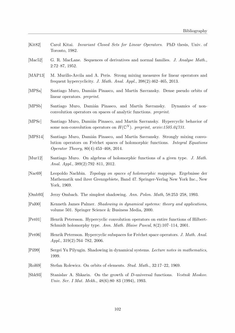
Bibliography

[Kit82] Carol Kitai. Invariant Closed Sets for Linear Operators. PhD thesis, Univ. of

Toronto, 1982.

[Mac52] G. R. MacLane. Sequences of derivatives and normal families. J. Analyse Math.,

2:72–87, 1952.

[MAP13] M. Murillo-Arcila and A. Peris. Strong mixing measures for linear operators and

frequent hypercyclicity. J. Math. Anal. Appl., 398(2):462–465, 2013.

[MPSa] Santiago Muro, Damian Pinasco, and Martın Savransky. Dense pseudo orbits of

linear operators. preprint.

[MPSb] Santiago Muro, Damian Pinasco, and Martın Savransky. Dynamics of non-

convolution operators on spaces of analytic functions. preprint.

[MPSc] Santiago Muro, Damian Pinasco, and Martın Savransky. Hypercyclic behavior of

some non-convolution operators on H(CN ). preprint, arxiv:1505.04731.

[MPS14] Santiago Muro, Damian Pinasco, and Martın Savransky. Strongly mixing convo-

lution operators on Frechet spaces of holomorphic functions. Integral Equations

Operator Theory, 80(4):453–468, 2014.

[Mur12] Santiago Muro. On algebras of holomorphic functions of a given type. J. Math.

Anal. Appl., 389(2):792–811, 2012.

[Nac69] Leopoldo Nachbin. Topology on spaces of holomorphic mappings. Ergebnisse der

Mathematik und ihrer Grenzgebiete, Band 47. Springer-Verlag New York Inc., New

York, 1969.

[Omb93] Jerzy Ombach. The simplest shadowing. Ann. Polon. Math, 58:253–258, 1993.

[Pal00] Kenneth James Palmer. Shadowing in dynamical systems: theory and applications,

volume 501. Springer Science & Business Media, 2000.

[Pet01] Henrik Petersson. Hypercyclic convolution operators on entire functions of Hilbert-

Schmidt holomorphy type. Ann. Math. Blaise Pascal, 8(2):107–114, 2001.

[Pet06] Henrik Petersson. Hypercyclic subspaces for Frechet space operators. J. Math. Anal.

Appl., 319(2):764–782, 2006.

[Pil99] Sergei Yu Pilyugin. Shadowing in dynamical systems. Lecture notes in mathematics,

1999.

[Rol69] Stefan Rolewicz. On orbits of elements. Stud. Math., 32:17–22, 1969.

[Shk93] Stanislav A. Shkarin. On the growth of D-universal functions. Vestnik Moskov.

Univ. Ser. I Mat. Mekh., 48(6):80–83 (1994), 1993.

102

Hiperciclicidad en espacios de funciones holomorfas y...

Documents

Transcript of Hiperciclicidad en espacios de funciones holomorfas y...