Localizability in κ-Minkowski Spacetime∗

Fedele Lizzi†1,2,3, Mattia Manfredonia‡1,2, and Flavio Mercati§1,2

1Dipartimento di Fisica “Ettore Pancini”, Universita di Napoli

Federico II, Napoli, Italy2INFN, Sezione di Napoli, Italy

3Departament de Fısica Quantica i Astrofısica and Institut de Cıencies

del Cosmos (ICCUB), Universitat de Barcelona, Barcelona, Spain

Abstract

Using the methods of ordinary quantum mechanics we study κ-Minkowski space as

a quantum space described by noncommuting self-adjoint operators, following and

enlarging [1]. We see how the role of Fourier transforms is played in this case by

Mellin transforms. We briefly discuss the role of transformations and observers.

∗Based on a talk given by FL at the XXVth edition of the conference in Vietri PAFT 2019, Current

problems in theoretical physics, to appear in the special issue dedicated to it.†fedele.lizzi@na.infn.it‡mattia.manfredonia@na.infn.it§flavio.mercati@gmail.com

1

arX

iv:1

912.

0709

8v1

[he

p-th

] 1

5 D

ec 2

019

The first quantum space has been the phase space of a point particle under quantiza-

tion. To study it, the tool which usually employed is due to Dirac, and is based on the

correspondence of position and momenta with noncommuting operator on the Hilbert

space of pure states. The commutation relation is given by

[qi, pj] = i~δij , (1)

where the dimensionful quantity ~ acts as deformation parameter. This quantum space is

extremely well known, and in the following we will recall some of its features as needed.

In this note we want to use similar methods, but apply them to a different space [2–12]:

κ-Minkowski spacetime. These methods have been useful for the study of the quantum

properties of various models of κ-Poincare invariant scalar field theories [10, 11]. Besides,

the geometric (spectral) properties, a la Connes, of the κ-Minkowski spacetime have

been investigated in [15–18]. defined by the following commutation relations in a four

dimensional spacetime:

[x0, xi] = iλxi, [xi, xj] = 0, (2)

where i, j = 1, 2, 3, x0 = c t with c speed of light, the deformation parameter λ has the

dimension of a length1 and time has a scale of λc. There exist many versions of ?-products

which reproduce the commutation relation (2), see e.g. [10,13,14]. Some of the results

collected here have been first present in [1], where further details can be found. The

κ-Minkowski space is the homogeneous space of the κ-Poincare Hopf algebra (quantum

group) [19–23]. κ-Minkowski is again a quantum space, but this time the deformation is

not of a phase space, and accordingly the deformation parameter is not the quantum of

action, but a length, which is natural to think of the order of Planck length, although

this is not strictly necessary.

Both non trivial commutation relations (1) and (2) give rise to uncertainty relations,

which are however quite different. In phase space we have

∆p∆q ≥ ~2

(3)

while in κ-Minkowski involves only a relation between the time coordinate and any of

the space ones,

∆x0∆xi ≥ λ

2|〈xi〉| , (4)

There is no uncertainty for measurement of space coordinates among themeselves.

1Often the deformation parameter λ is indicated by 1κ , hence the name.

2

We follow this analogy and apply Dirac’s correspondence principle to study the

kinematics of a spacetime “quantized” by λ (as phase space was quantized by ~). In the

end of the paper are going to briefly discuss how measurements of position and time are

concerned in such a framework, and which are the states. One might wonder whether

localizability of a state depend on the reference frame or not. As an example, for the

quantum phase space of one particle the algebra of positions and momenta is invariant

under classical translations and rotations. However, the algebra (2) is clearly not invariant

under the classical action of the Poincare group (in particular under translations and

boosts) but it is under a deformation of the Poincare group. This makes the group

manifold itself into a noncommutative space, as a consequence, different observers will

not agree in general on the localizability properties of the same state. We stress that in

the present we will strictly discuss the kinematics of systems in κ-Minkowski but not their

dynamics. We are interested in the relation between the noncommutativity of spacetime

and the localizability of events, independently of the dynamical laws they are subject

to. The limits to localizability then could be understood as the effective description of

gravitational excitations that intervene when enough energy is concentrated into a small

region in order to localize an event [24, 25], and this would indeed be a dynamical effect.

This connection with a fundamental quantum field theory of gravity is only crude. At

the moment it can be made precise in 2+1 dimensions where relations like (2) emerge

once one integrate away the gravitational degrees of freedom in a model of quantum

gravity coupled with matter [26,27].

Example: Quantum Phase Space for a particle in 3D

We shortly discuss the archetypical noncommutative geometry of the phase space of a

single quantum particle in three dimension. The material is known from elementary

courses in quantum mechanics, but we wish to stress a few features which will be used

analogously for κ-Minkowski spacetime. The quantization turns the coordinates (qi, pi)

of the six-dimensional phase space into noncommuting operators: qi and pi. These

are commonly represented as operators on the Hilbert spaceL2(R3q) of square integrable

functions of space as2:

qiψ(q) = qiψ(q) ; piψ(q) = −i~∂

∂qiψ(q) . (5)

2To simplify the notation we indicate by q and p the corresponding three-vectors, avoiding the use of

a notation like ~q.

3

They are unbounded selfadjoint operators with a dense domain. The spectrum is the

real line (for each i). The eigenvalue equation

∂qψ(q) = αψ(q) , α ∈ C3 (6)

admits only improper eigenfunctions eα·q with α = ik a pure imaginary number. We all

know that those are physically interpreted as infinite plane waves of given a frequency.

As usual |ψ(q)|2 for normalized functions gives the probability density to find the particle

at position q. The wave function, being a complex quantity, contains also the information

about the density probability of the momentum operator.

If we choose the pi as the complete set of observable, we have

qiφ(p) = i~∂

∂piφ(p) ; piφ(p) = piφ(p) . (7)

Of course, ψ(q) and φ(p) carry exactly the same information and are connected by a

Fourier transform3:

ψ(q) =1

(2π)32

∫d3p φ(p)e

i~p·q (8)

This is of course well known. Let us now consider the case of κ-Minkowski in the same

spirit.

Time and position of events in κ-Minkowski space

Let us begin by considering the xi’s as a complete set of observables on the Hilbert space

L2(R3x). We will represent4 the xµ as operators on this space as5

xiψ(x) = xiψ(x),

x0ψ(x) = iλ

(∑i

xi∂xi +3

2

)ψ(x) = iλ

(r∂r +

3

2

)ψ(x). (9)

The 32

factor is necessary to have symmetric operators. Here, x0 plays the role that p

played in quantum phase space. The x0 operator is a dilation operator, and this suggests

the use of a polar basis. The polar coordinates θ, ϕ do not correspond to well defined

self-adjoint operators, but if one defines r cos θ = x3 and r eiϕ = (x1 + ix2), then gets

[x0, cos θ] = [x0, eiϕ] = 0 , [x0, r] = iλr . (10)

3It is important that the Fourier transform is an isometry, i.e. it maps normalized functions of

positions into normalized functions of momenta.4 The representations of the algebra generated by (2) are discussed in detail in [28,29]5The most general class of operator compatible with the algebra can be found in [30](see also [31,32])

4

In fact x0 commutes with all spherical harmonics, or in general functions of θ and ϕ

independent on r. In the following we will consider the vectors of L2(R3x) to be functions

of the kind ψ =∑

lm ψlm(r)Ylm(θ, ϕ). Moreover, since the angular variables commute

with everything, we will focus on the radial part only. The uncertainty relation (4) can

be expressed in its polar version

∆x0∆r ≥ λ

2|〈r〉|. (11)

The operator x0 is symmetric, but we should verify its self-adjointness domain.

Integrating by parts, one finds:∫drr2 ψ∗1iλ

(r∂r +

3

2

)ψ2 = iλ

∫drr2 ψ∗1

3

2ψ2−

∫dr iλ∂r

(r3ψ∗1

)ψ2 +ψ∗1r

3ψ2

∣∣∣∣∞0

. (12)

One can see that the boundary term vanishes if ψ1 and ψ2 vanish at infinity faster than

r−32 , which is true for all square-integrable (according to the measure

∫drr2) functions. In

the origin the condition imposed is weaker than the one imposed by square-integrability.

Let us now look for the spectrum and the (improper) eigenvectors. Monomial in r are

formal solutions of the eigenvalue problem:

iλ

(r∂r +

3

2

)rα = iλ(α +

3

2)rα = λαr

α, (13)

therefore eigenvalues are

λα = iλ(α +3

2). (14)

Monomials are never acceptable physical states, vector of L2(R3x). They are never square

integrable becasue they will always diverge either at the origin or at infinity (remember

the correct measure!). When the real part of α = −32

the function diverges both at zero

and at infinity. Compare this with plane waves. An exponential, which is the formal

solution of the eigenvalue equation for momentum, also diverges either at plus or minus

infinity. When the exponential is pure imaginary it diverges at both ends, but only

marginally, i.e. in a way that it is a good distribution with a large dens domain. In this

case also the eigenvalues are real, as it befits to a self-adjoint operator. This behaviour is

mirrored in the κ-Minkowski case. Eigenfunctions (13) are acceptable distributions if

and only if

α = −3

2+ iτ, τ ∈ R (15)

The spectrum of the time operator is real and goes from minus infinity to plus infinity.

What plane waves were for momentum in quantum phase space, now are the distribution

5

Tτ =r−

32−iτ

λ−iτ= r−

32 e−iτ log( rλ), (16)

They have a well defined inner product with every vector in the domain of x0. The

distribution has the correct dimension of a length to the 3/2, the factor of λ is there to

avoid taking the logarithm of a dimensional quantity.

The operator x0 is selfadjoint, therefore the Tτ are a complete base. Both r, θ, ϕ and

τ, θ, ϕ are complete sets of observables. Completeness implies that any function of r can

be isometrically expanded in terms of the Tτ .

ψ(r, θ, ϕ) =1√2π

∫ ∞−∞

dτ r−32 e−iτ log( rλ)ψ(τ, θ, ϕ) =M−1

[ψ(τ, θ, ϕ), r

], (17)

ψ(τ, θ, ϕ) =1√2π

∫ ∞0

dr r12 eiτ log( rλ)ψ(r, θ, ϕ) =M

[ψ(r, θ, ϕ),

3

2+ iτ

]. (18)

The above integrals define a Mellin transform together with its inverse. Both are

isometries between square integrable functions of r with measure drr2 and functions of τ .

We see that Mellin transform are for k-Minkowski what Fourier are for quantum phase

space. Hereafter we will often omit the explicit dependence on θ and ϕ when there is no

confusion.

We are now going to make an important assumption: that the usual theory of

measurement holds. Namely, observables are self-adjoint operator, bounded or unbounded.

The possible results of a measurement are the points of the spectrum, and when a pure

state is expressed in the spectral decomposition given by the complete set of (proper or

improper) eigenfunctions of the observables, the modulus square of the function gives the

probability density. With these assumptions, the average time measured by a particle in

the state described by ψ with spherical symmetry gives:

〈x0〉ψ = 4π

∫r2drψ(r)iλ

(r∂r +

3

2

)ψ(r) (19)

If ψ is real it results 〈x0〉ψ = 0. Hence only complex valued functions will have non

vanishing mean value of time (in analogy with quantum phase space, where real functions

have a vanishing mean value of the momentum). The probability of measuring a given

value of τ is given by |ψ(τ)|2 for normalised functions.

To have a feeling for the dimensional quantities consider λ to be Planck length.

Reinserting dimensionful quantities τ = t cλ

with t = x0

c. If t = 1 s, then τ = 2 · 1043, an

extremely large number. If t is of the order of Planck time, then τ ∼ 1.

6

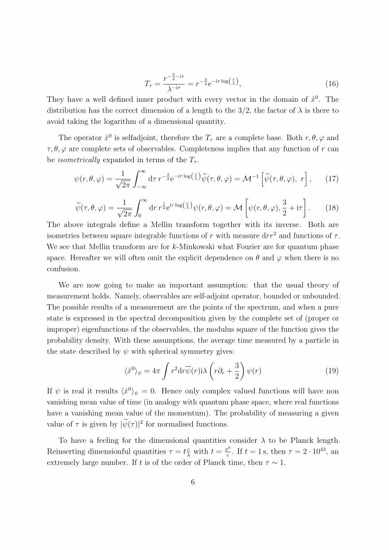
Various examples of functions can be found in [1], here we present some further

examples of localization of states in space and time. In the following we will consider

only the radial coordinate, since, as we said, the angular part does not play any role.

We first note that according to (11) it is possible to localize a particle both in space

and time, as long as the position is the origin. Such a state, being akin to a Dirac’s δ,

will again be a distribution, but we can present it as limit of ordinary states. To do so we

use functions that saturate the uncertainty bounds provided by (11) (i.e. the analogue

of what Gaussian coherent states were for quantum phase space). It turns out that this

role is played by normalized log-Gaussians, plotted in Fig. 1,

L(r, r0) = Ne−(log r−log r0)

2

σ2 =e−(

log( rr0 )σ

)2

e−916σ2

√σ(2π)3/4

√r3

0

. (20)

These functions have a maximum in r = r0, and they localize at r = r0 as σ → 0, and at

r = 0 as r0 → 0, for any value of σ ≥ 0 and are plotted in Fig. 1.

σ=2.5

σ=2

σ=1.5

σ=1

σ=0.5

0.0 0.5 1.0 1.5 2.0r

2

4

6

8

10

L(r,r0) r0=exp -σ 2.01

Figure 1: The σ →∞ limit of L(r, r0) when ξ = e−σ(2+ε)

, for ε = 0.01.

The Mellin transform (18) of these states is a Gaussian:

L(τ, r0) =σ

12 e−

14σ2τ(τ−3i)

2 4√

2π3/4

(r0

λ

)iτ

, (21)

With square norm: ∣∣∣L(τ, r0)∣∣∣2 =

σe−σ2τ2

2

4√

2π3/2, (22)

7

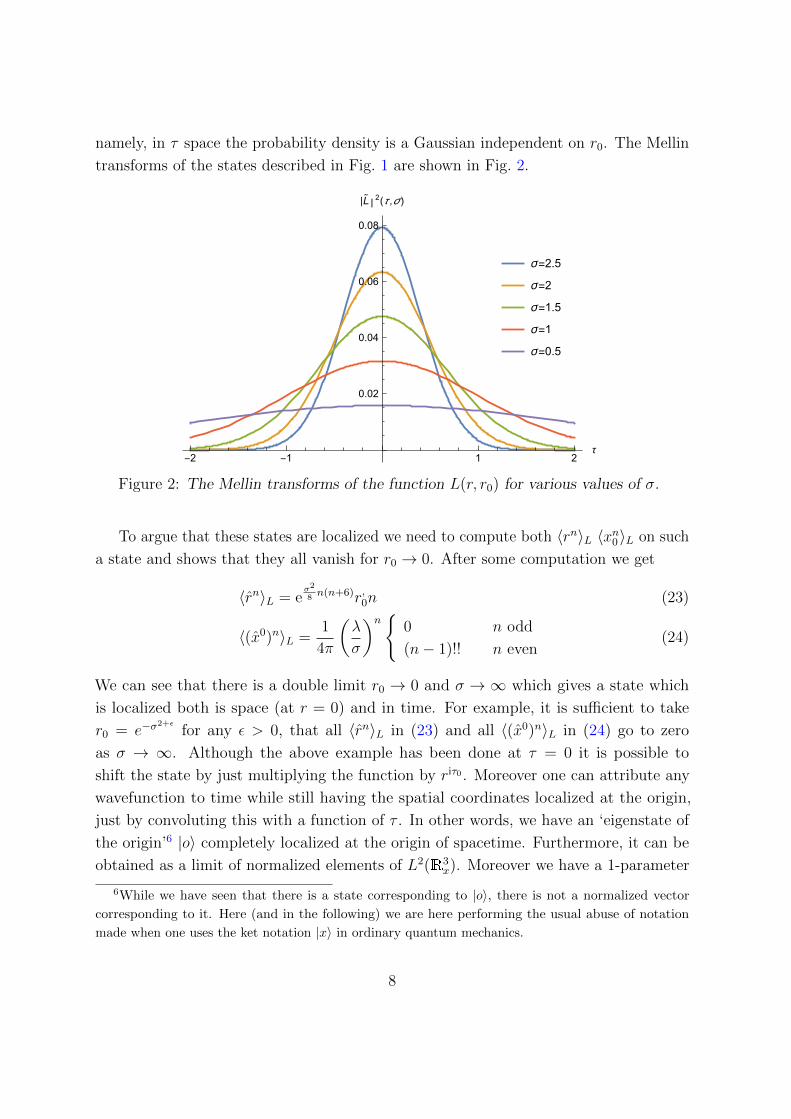
namely, in τ space the probability density is a Gaussian independent on r0. The Mellin

transforms of the states described in Fig. 1 are shown in Fig. 2.

σ=2.5

σ=2

σ=1.5

σ=1

σ=0.5

-2 -1 1 2τ

0.02

0.04

0.06

0.08

|L˜ 2(τ ,σ )

Figure 2: The Mellin transforms of the function L(r, r0) for various values of σ.

To argue that these states are localized we need to compute both 〈rn〉L 〈xn0 〉L on such

a state and shows that they all vanish for r0 → 0. After some computation we get

〈rn〉L = eσ2

8n(n+6)r,0n (23)

〈(x0)n〉L =1

4π

(λ

σ

)n{0 n odd

(n− 1)!! n even(24)

We can see that there is a double limit r0 → 0 and σ → ∞ which gives a state which

is localized both is space (at r = 0) and in time. For example, it is sufficient to take

r0 = e−σ2+ε

for any ε > 0, that all 〈rn〉L in (23) and all 〈(x0)n〉L in (24) go to zero

as σ → ∞. Although the above example has been done at τ = 0 it is possible to

shift the state by just multiplying the function by riτ0 . Moreover one can attribute any

wavefunction to time while still having the spatial coordinates localized at the origin,

just by convoluting this with a function of τ . In other words, we have an ‘eigenstate of

the origin’6 |o〉 completely localized at the origin of spacetime. Furthermore, it can be

obtained as a limit of normalized elements of L2(R3x). Moreover we have a 1-parameter

6While we have seen that there is a state corresponding to |o〉, there is not a normalized vector

corresponding to it. Here (and in the following) we are here performing the usual abuse of notation

made when one uses the ket notation |x〉 in ordinary quantum mechanics.

8

family of states, |oτ 〉 localized at the origin of space at a nonzero time. These states as

well can be obtained as limits of normalized elements of L2(R3x).

Alternatively one can consider states which are Gaussian in position (not log-Gaussian).

The presence of a cusp in the origin does not pose problems since we are not requiring

differentiability, at any rate it can be smoothened if necessary. States of the kind

G(r, r0, σ) = Ne(r−r0)

2σ (25)

with the normalization

N−2 =1

2

√πσ(

erf(r0

σ

)+ 1)

(26)

have tranform

G(r, r0, σ) =

N(λσ )

−iτ(σΓ( iτ

2+ 3

4) 1F1

(− iτ

2− 1

4; 12

;− r20σ2

)+2r0Γ( it2 + 5

4) 1F1

(14− iτ

2; 32

;− r20σ2

))√

2π√σ(erf( r0σ )+1)

(27)

where 1F1 are hypergeometric functions of the first kind.

The analogues of Figs. 1 and 2 are in Figs. 3 and 4 respectively.

σ=2.5

σ=2

σ=1.5

σ=1

σ=0.5

2 4 6 8 10r

0.2

0.4

0.6

0.8

G(r,r0,σ )

r0

Figure 3: The function G(r, r0) for various values of σ.

Note that in both cases the constant λ appears only as a phase, and will not appear

in the modulus square of the function. It is nevertheless impossible to set λ = 0 from the

onset, as it would give singular functions without a definite limit.

9

σ=2.5

σ=2

σ=1.5

σ=1

σ=0.5

-10 -5 5 10τ

0.5

1.0

1.5

2.0

2.5

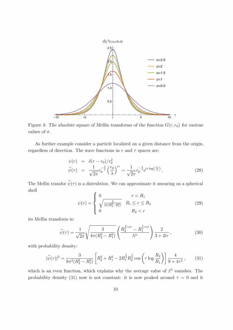
|G˜ 2(τ,r0=3,σ )

Figure 4: The absolute square of Mellin transforms of the function G(r, r0) for various

values of σ.

As further example consider a particle localized on a given distance from the origin,

regardless of direction. The wave functions in r and τ spaces are:

ψ(r) = δ(r − r0)/r20

ψ(τ) =1√2πr− 3

20

(r0

λ

)iτ

=1√2πr− 3

20 eiτ log( r0λ ) , (28)

The Mellin transfor ψ(τ) is a distrubtion. We can approximate it smearing on a spherical

shell

ψ(r) =

0 r < R1√

34π(R3

2−R31)

R1 ≤ r ≤ R2

0 R2 < r

(29)

its Mellin transform is:

ψ(τ) =1√2π

√3

4π(R32 −R3

1)

(R

32

+iτ

2 −R32

+iτ

1

λiτ

)2

3 + 2iτ, (30)

with probability density:

|ψ(τ)|2 =3

8π2(R32 −R3

1)

[R3

2 +R31 − 2R

321R

322 cos

(τ log

R2

R1

)]4

9 + 4τ 2, (31)

which is an even function, which explains why the average value of x0 vanishes. The

probability density (31) now is not constant: it is now peaked around τ = 0 and it

10

decreases like τ−2 away from the origin. In the limit R1 → R2 the Mellin transform (30)

is (up to a constant) the Mellin transform of the delta function, (28).

Note that in all these examples, when the particle is localised, even if on a spherical

shell, the square of the wave function |ψ(τ)|2 is independent on τ . Localization in space

means complete delocalization in time. This is a consequence of the uncertainty, just as

phase space the Fourier transform of localised states (Dirac’s δ) are plane wave, whose

suare modulus does not depend on the momentum.

Is the origin special?

We have argued that the origin is a special point. Does this mean that somewhere in

the universe there is “the origin”. A special position in space singled out by the κ-God?

Needless to say, there is no special point, and the space is “translationally invariant”.

The invariance is however not under the usual Poincare group, but under the quantum

symmetry called κ-Poincare. This issue is described in detail in [1]. Here we will give a

shortened version.

Implicitly in our discussion, when we were referring to states we were assuming the

existence of an observer measuring the localisation of states. This observer is located

at the origin, and he can measure with absolute precision where he is. For him “here”

and “now” make sense. He cannot localize with precision states away from him, as a

consequence of the noncommutativity of κ-Minkowski. What about other observers? A

different observer will be in general Poincare transformed, i.e. translated, rotated and

boosted. These operations are usually performed with an element of the Poincare group.

One motivation to introduce κ-Minkowski is its relations to the quantum group

κ-Poincare. We should therefore use deformed transformations. We require invariance

under the transformation xµ → x′µ = Λµν ⊗ xν + aµ ⊗ 1. The commutations relations in

a particular basis [9, 21] are:

[aµ, aν ] = iλ (δµ0 aν − δν0 a

µ) , [Λµν ,Λ

ρσ] = 0

[Λµν , a

ρ] = iλ [(Λµσδ

σ0 − δµ0) Λρ

ν + (Λσνδ

0σ − δ0

ν) ηµρ] (32)

With coproduct, antipode and counit

∆(aµ) = aν ⊗ Λµν + 1⊗ aµ , ∆(Λµ

ν) = Λµρ ⊗ Λρ

ν ,

S(aµ) = −aν(Λ−1)µν , S(Λµν) = (Λ−1)µν , ε(a

µ) = 0 , ε(Λµν) = δµν (33)

11

We represented the κ-Minkowski algebra as operators. But in doing so we had

implicitly chosen an observer. In order to take into account the fact that there are

different observers we enlarge the the algebra (and consequently the space) to include

the parameters of the new observers. We call then new set of states as Pκ. Observers

in this space cannot prescind from quantization, there are not “classical” observers in

κ-Minkowski. Our (generalized) Hilbert space will now comprise not only function on

spacetime (either functions of r or τ), but also functions of the a’s and Λ’s.

We can represent the κ-Poincare group translations faithfully as

aρ = −iλ

2

[(Λµ

σδσ

0 − δµ0) Λρν +

(Λσ

νδ0σ − δ0

ν

)ηµρ]

Λνα

∂

∂ωµα

+iλ

2

(δρ0 q

i ∂

∂qi+ δµi q

i

)+

1

2h.c. (34)

while the Λ’s are simply represented as multiplicative operators.

Therefore that, like spacetime, the space of observers is also noncommutative, but

the noncommutativity is only present in the translation sector. This the observers

counterpart of the fact that the angular variables commute with everything. Observers

which differ only for a rotation will agree on everything. Boosted observes will not, since

a boost involves time, which is a quantized variable. Let us further explore the space

of observers, seen as states. First consider the observer located at the origin, which is

reached via the identity transformation. Define |o〉P of with the property:

P〈o| f(a,Λ)|o〉P = ε(f) , (35)

with f(a,Λ) a generic noncommutative function of translations and Lorentz transforma-

tion matrices, and ε the counit. This state describes the Poincare transformation between

two coincident observers. The state is such that all combined uncertainties vanish.

Coincident observers are therefore a well-defined concept in κ-Minkowski spacetime. A

change of observer will transform xµ → x′µ = Λµν ⊗ xν + aµ ⊗ 1, primed and unprimed

coordinates correspond to different observers. Identifying x with 1⊗ x we generate an

extended algebra P ⊗M which extends κ-Minkowski by the κ-Poincare group algebra.

This algebra takes into account position states and observables. It is a noncommutative

algebra, as it befits to noncommutative observers. Just as we cannot sharply localize

position states, neither we can sharply localize where the observer is.

We can build the action of the position, translation and Lorentz transformations

operator on generic functions of all those variables. Let us just state a result, as an

12

example, sending to [1] for further details. Poincare transforming the origin state |o〉 by

wavefunction |g〉 in the representation of aµ,Λµν we obtain for all polynomials in the

transformed coordinates

x′µ = aµ ⊗ 1 + Λµν ⊗ xν (36)

the same expectation value as the one assigned by |g〉 to the corresponding polynomials

in aµ. In other words, the state of x′µ is identical to the state of aµ. Uncertainty ∆x′µ

is introduced by the uncertainty of the aµ close a noncommutative algebra, we cannot

know, with absolute precision where the new observer is.

Challenges

Here we discussed purely the kinematics of κ-Minkowski. To discuss dynamics, at a

quantum level, we would have to introduce phase space, and momentum. The latter is a

most interesting object in this case, the space of momenta is curved [33–35]. Although

the noncommutativity of translations, and the nontrivial curvature of momenta are both

aspect of the quantum nature of κ-Minkowski and κ-Poincare, it is not immediate to see

momenta as generator of translations in an operatorial way. The connection is subtle

and some aspects are being investigate in [36]. Since the observers are indetermined, as

well as the states, there is the issue of the possibility of defining in a meaningful way

the cluster decomposition principle, or at least meaningful Pauli-Jordsn functions in this

context [37]. A noncommutative geometry has, by nature, some degree of nonlocality,

but is necessary to understand in which way the scale and the details of this nonlocality

can be made compatible with quantum field theory.

Acknowledgements

FL and MM acknowledge the support of the INFN Iniziativa Specifica GeoSymQFT; FL

the Spanish MINECO under project MDM-2014-0369 of ICCUB (Unidad de Excelencia

‘Maria de Maeztu’): FM the Action CA18108 QG-MM from the European Cooperation

in Science and Technology (COST) and partial support from the Foundational Questions

Institute (FQXi).

13

References

[1] F. Lizzi, M. Manfredonia, F. Mercati and T. Poulain, “Localization and Refer-

ence Frames in κ-Minkowski Spacetime,” Phys. Rev. D 99 (2019) no.8, 085003

doi:10.1103/PhysRevD.99.085003 [arXiv:1811.08409 [hep-th]].

[2] S. Majid, and H. Ruegg, “Bicrossproduct structure of κ-Poincare group and non-

commutative geometry” Phys. Lett. B334 (1994) 348, hep-th/9405107v2.

[3] S. Majid, “Algebraic approach to quantum gravity II: noncommutative spacetime,”

in D. Oriti (ed.): Approaches to quantum gravity, Toward a New Understand-

ing of Space, Time and Matter, pp. 466–492, Cambridge University Press (2009),

arXiv:hep-th/0604130.

[4] P. Kosinski, P. Maslanka, J. Lukierski, and A. Sitarz, “Generalized κ deformations

and deformed relativistic scalar fields on noncommutative Minkowski space,” in

Mexico City 2002, Topics in mathematical physics, general relativity and cosmology,

pp. 255–277 (2003), arXiv:hep-th/0307038.

[5] P. Kosinski, J. Lukierski, and P. Maslanka, “Local D= 4 field theory on κ-deformed

Minkowski space,” Phys. Rev. D62 no. 2, (2000) 025004, arXiv:hep-th/9902037.

[6] M. Dimitrijevic, L. Jonke, L. Moller, E. Tsouchnika, J. Wess, and M. Wohlgenannt,

“Deformed field theory on kappa space-time,” Eur. Phys. J. C31 (2003) 129–138,

arXiv:hep-th/0307149 [hep-th].

[7] M. Arzano, J. Kowalski-Glikman, and A. Walkus, “Lorentz invariant field theory

on κ–Minkowski space,” Class. Quant. Grav. 27 (2010) 025012, arXiv:0908.1974

[hep-th].

[8] F. Mercati, “Quantum κ-deformed differential geometry and field theory,” Int. J.

Mod. Phys. D25, (2016) 1650053, arXiv:1112.2426 [math.QA].

[9] F. Mercati, and M. Sergola, “Light Cone in a Quantum Spacetime,” Phys. Lett.

B787, (2018) 105–110, arXiv:1810.08134 [hep-th].

[10] T. Poulain, and J.-C. Wallet, “κ-Poincare invariant quantum field theories with

Kubo-Martin-Schwinger weight,” Phys. Rev. D98, (2018) 025002, arXiv:1801.02715

[hep-th].

14

[11] T. Poulain, and J.-C. Wallet, “κ-Poincare invariant orientable field theories at 1-loop:

scale-invariant couplings,” arXiv:1808.00350 [hep-th].

[12] F. Lizzi, P. Vitale and A. Zampini, “The fuzzy disc: A review,” J. Phys. Conf. Ser.

53 (2006) 830.

[13] B. Durhuus and A. Sitarz, “Star product realizations of kappa-Minkowski space,” J.

Noncommut. Geom. 7 (2013) 605, arXiv:1104.0206 [math-ph].

[14] S. Meljanac and S. Kresic-Juric, “Generalized kappa-deformed spaces, star-products,

and their realizations,” J. Phys. A 41 (2008) 235203, arXiv:0804.3072 [hep-th].

[15] F. D’Andrea, “Spectral geometry of κ-Minkowski space,” J. Math. Phys. 47 (2006)

062105, arXiv:hep-th/0503012.

[16] B. Iochum, T. Masson, T. Schucker, and A. Sitarz, “Compact κ-Deformation and

Spectral Triples,” Rept. Math. Phys. 68 (2011) 37-64, arXiv:1004.4190 [hep-th].

[17] B. Iochum, T. Masson, and A. Sitarz, “κ-deformation, affine group and spectral

triples,” Banach Center Publ. 98 (2012) 261–291, arXiv:1208.1140 [math-ph].

[18] M. Matassa, “A modular spectral triple for κ-Minkowski space,” J. Geom. Phys. 76

(2014) 136, arXiv:1212.3462 [math-ph].

[19] J. Lukierski, H. Ruegg, A. Nowicki, and V. N. Tolstoy, “q-deformation of Poincare

algebra,” Phys. Lett. B264, (1991) 331–338.

[20] J. Lukierski, A. Nowicki, and H. Ruegg, “New quantum poincare algebra and

κ-deformed field theory,” Phys. Lett. B293, (1992) 344–352.

[21] S. Zakrzewski. “Quantum poincare group related to the kappa-poincare algebra,” J.

Phys. A27, (1994) 2075.

[22] J. Lukierski and H. Ruegg, “Quantum κ-Poincare in any dimension,” Phys. Lett.

B329, (1994) 189–194, arXiv:hep-th/9310117.

[23] F. Mercati and M. Sergola, “Physical Constraints on Quantum Deformations of

Spacetime Symmetries,” Nucl. Phys. B933, (2018) 320–339, arXiv:1802.09483

[hep-th].

15

[24] S. Doplicher, K. Fredenhagen, and J. Roberts “The quantum structure of spacetime

at the Planck scale and quantum fields,” Comm. Math. Phys. Volume 172, Number

1 (1995), 187-220, arXiv:0303037v1 [hep-th].

[25] C. Alden Mead “Possible Connection Between Gravitation and Fundamental Length,”

Phys. Rev. 135, B849(1969).

[26] L. Freidel and E. R. Livine “3d Quantum Gravity and Effective Non-Commutative

Quantum Field Theory ,” Phys. Rev. Lett. 96, 221301 (2006), arXiv:0512113v2

[hep-th].

[27] H.-J. Matschull and M. Welling “Quantum Mechanics of a Point Particle in 2+1

Dimensional Gravity,” Class.Quant.Grav. 15 (1998) 2981-3030, arXiv:9708054v2

[gr-qc].

[28] A. Agostini, “kappa-Minkowski representations on Hilbert spaces,” J. Math. Phys.

48 (2007) 052305, arXiv:hep-th/0512114.

[29] L. Dabrowski and G. Piacitelli, “Canonical k-Minkowski Spacetime,”

arXiv:1004.5091 [math-ph].

[30] S. Meljanac and M. Stojic, “New realizations of Lie algebra kappa-deformed Eu-

clidean space,” Eur. Phys. J. C 47 (2006) 531, arXiv:hep-th/0605133.

[31] S. Meljanac, D. Meljanac, F. Mercati and D. Pikutic, “Noncommutative spaces and

Poincare symmetry,” Phys. Lett. B766 (2017) 181, arXiv:1610.06716 [hep-th].

[32] N. Loret, S. Meljanac, F. Mercati and D. Pikutic, “Vectorlike deformations of

relativistic quantum phase-space and relativistic kinematics,” Int. J. Mod. Phys.

D26 (2017) 1750123, arXiv:1610.08310 [hep-th].

[33] J. Kowalski-Glikman and S. Nowak, “Doubly special relativity and de Sitter space,”

Class. Quant. Grav. 20 no. 22, (2003) 4799, arXiv:hep-th/0304101.

[34] M. Arzano, “Anatomy of a deformed symmetry: Field quantization on curved

momentum space,” Phys. Rev. D83 (2011) 025025, arXiv:1009.1097 [hep-th].

[35] G. Gubitosi and F. Mercati, “Relative locality in κ-Poincare,” Class. Quant. Grav.

30 no. 14, (2013) 145002, arXiv:1106.5710 [gr-qc].

[36] F. Lizzi, M. Manfredonia, F. Mercati, “Momentum Space for κ-Minkowski space-

time”, in preparation.

16

[37] F. Mercati and M. Sergola, “Pauli-Jordan Function and Scalar Field Quantiza-

tion in κ-Minkowski Noncommutative Spacetime,” Phys. Rev. D98 (2018) 045017,

arXiv:1801.01765 [hep-th].

17