Presentation Finalfinal

A Model of Unconventional Monetary Policyby M. Gertler and P. Karadi

Donat Bunger Melika Liporace

HEC Lausanne

May 20, 2014

Business Cycles Unconventional monetary policy May 20, 2014 1 / 32

Outline

1 Introduction

2 Model SetupBasic FrameworkAgents’ Characteristics

3 Model AnalysisCrisis ExperimentCredit PolicyCredit Policy with Zero Lower BondWelfare

4 ConclusionResultsCritics


Introduction

Introduction

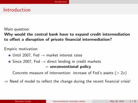
Main question:Why would the central bank have to expand credit intermediationto offset a disruption of private financial intermediation?

Empiric motivation:

Until 2007, Fed → market interest rates

Since 2007, Fed → direct lending in credit markets= unconventional policy

Concrete measure of intervention: increase of Fed’s assets (> 2x)

⇒ Need of model to reflect the change during the recent financial crisis!


Introduction

Introduction

Previous litterature:

Model of conventional monetary policy:→ Frictionless financial market ⇒ no financial market disruption→ No motivation for unconventional policy

Model with frictions in financial market:→ Unconventional monetary policy not allowed in model

Model with unconventional monetary policy:→ No quantitative model (qualitative analysis)

Aim:

Develop quantitative macro-model allowing unconventional policies

Analyze unconventional policy effects in a ”regular” macro-framework

NOT to model sub-prime crisis


Introduction

Introduction

Key elements of the sub-prime crisis:

7−→ Sharply reduced asset values

⇒ Weakend balance sheets of financial intermediaries

⇒ Disruptions in the flow between lenders and borrowers by sharprises in various credit spreads

⇒ Significantly tightened lending standards

⇒ Increased borrowing costs

⇒ Enhanced downturn

⇒ Contraction in the real economy

⇒ Reduced asset values of intermediaries

⇒ ... and so on


Introduction

Introduction

Particularities of the model:

Agency problem: the banker can steal

⇒ Endogenous constraints on ratio between bank’s equity and deposits⇒ Tying of credit flows to the equity capital⇒ Disruption of lending and borrowing⇒ Credit costs are raised

Central bank subsitutes to private financial sector:

⇒ Central bank borrows/lends, but cannot steal⇒ No constraints on leverage ratio⇒ Optimal (less suboptimal) investments


Model Setup Basic Framework

Model SetupBasic Framework

DSGE model with nominal rigidities

Explicit modelisation of financial intermediaries

→ Agency problem ⇒ additional constraint

Shocks on capital quality (vs. usually technological shocks)

6 agents:I Housholds

F WorkersF Bankers

I Financial intermediariesI Intermediates goods firmsI RetailersI Capital producing firmsI Government


Model Setup Agents’ Characteristics

Model SetupAgents’ Characteristic: Households

Labor dynamics:

Fixed fraction of bankers and workersPossible switching between occupationsProbability θ to stay banker

Money dynamics:

One period bondsRiskless return Rt

(In equilibrium) intermediary deposit ⇔ government debtNeither MIU nor CIA (here, agency problem limits money exchanged)

Then: usual optimization problem

Utility function U(Ct ,Ct−1, Lt)Budget constraint Ct = WtLt + Πt + Tt + RtBt − Bt+1

⇒ ET and FOC



Model SetupAgents’ Characteristic: Banks

Claims’ (from producing firms) composition (balance sheet of agent j):

claims’ total value = deposits + equityQtSj ,t = Bj ,t+1 + Nj ,t

Financial parameters:

Stochastic discount (in t for t + i): βi · marginal utility of Ct

marginal utility of Ct+1+i

Net returns on assets: (Rkt+1+i − Rt+1+i )

⇒ (1) banker enters if: expectation of the discounted premium ≥ 0

Stealing process:

Household recovers a share 1− λ of banks’ assetsBanker gets a share λ and goes bankruptcy⇒ (2) houshold enters if: no incentive for the banker to steal:

Vj,t ≥ λQtSj,t




Now, from maximisation of expected final wealth, we can express:

Vj ,t = νtQtSj ,t + ηtNj ,t

where:I νt : expected discounted marginal gain to expand assetsI ηt : expected discounted marginal gain to expand equity

Effect of constraint (2) Vj ,t ≥ λQtSj ,t :

Not binding ⇒ νt = 0 (no financial friction, usual model)

Binding ⇒ QtSj ,t = ηtλ−νt Nj ,t = φtNj ,t (φt : leverage ratio)

We then find:QtSt = φtNt

→ assets constraint by bank’s equity




Law of motion of equity:

Individually:equity = gross profits - debtsNj,t+1 = Rk

t+1QtSj,t - Rt+1Bj,t+1

We then find:

Nj ,t+1 =[(Rk

t+1 − Rt+1)φt + Rt+1

]Nj ,t

On the whole sector:I Surviving bankers: fraction θ of survivng bankers’ wealth Nj,t+1

I Entering bankers: fraction ω1−θ of exiting bankers’ wealth (1− θ)QtSt−1

We then find:

Nt+1 = θ[(Rk

t+1 − Rt+1)φt + Rt+1

]Nt + ωQt+1St



Model SetupAgents’ Characteristic: Intermediate Goods Firms

Production function: Yt = At(UtξtKt)αL1−αt

ξt : quality of capital ⇒ ξtKt : effective capital

→ Aim: provide exogenous variation of capital value

Ut utilization rate of capital, choice variable

Kt financed by claims, priced at capital price ⇒ QtKt+1 = QtSt

→limited by friction from agency problemThen, usual FOC

Profits:No profits state by state ⇒ returns paid to bank, Rk

t = returns on capital

Note: no friction here, no cheating between banks and firms



Model SetupAgents’ Characteristic: Government

Problem:Shock in capital quality

==⇒ shock in capital returns==⇒ shock in banks’ returnsloss

==⇒ shock in equityconstraint

======⇒ underoptimal investments

⇒ Unconventional monetary policy: government acts as banks

Borrow from household, Rt

Lend to producing firms, Rkt

BUT no possibility of diverting money ⇒ no agency problem constraint

BUT efficiency costs: τ/unit supplied




Concretely:

Central bank funds a fraction ψ of intermediated assets, which describesthe intensity of central bank’s fight again financial crisis

⇒ QtSt = φtNt + ψtQtSt = 11−ψt

φtNt

Government budget:

(Additional) expenditures: τψtQtKt+1

(Additional) revenues: (Rkt − Rt)Bg ,t−1




Central bank rules:

In normal times: simple Taylor rule, with interest-rate smoothing

In crisis: no interest-rate smoothing and credit injection:

ψt = ψ + vEt

[(logRk

t+1 − logRt+1)− (logRkSS − logRSS)

]I Feedback parameter, v , positiveI Credit expansion when spread increase w.r.t its steady-state value



Model SetupAgents’ Characteristic: Other Agents

Capital producing firms:

Allow real differentiation: consumption good vs. capital→ very expensive to transform one into the other

Maximizing profits sets the price of capital

Any profit goes as lump-sum to households

No real essential feature for our analysis here

Retail firms:

Introduce nominal rigidities and inflation

Very similar to NKBC model features


Model Analysis

Model Analysis

We show three different simulations of crisis:

1 Basic experiment without government intervention

2 Central bank intervention by credit policy

3 Central bank intervention by credit policy, with zero lower bound

Note: Conventional values are used for the calibrated parameters

(β, θ, λ, ω, Taylor rule parameters, etc.)


Model Analysis Crisis Experiment

Model AnalysisCrisis Experiment

Simple example: asset price shock during sub-prime

Introduction Systemic Risk Contagion

Contagion through Asset Prices: Example

• Capital requirement:

Equity

Total Assets

!≥ 10%

• Two banks of equal size, A and B,holding the same type of assets

• Bank A’s equity exceeds the capitalrequirement by 50%

• Bank B’s equity just meets thecapital requirement

32 / 43

→


Contagion through Asset Prices: Illustration

• Now, asset prices drop by 5%

• Bank A loses 1/3 of its equity butstill meets the capital requirement

• Bank B loses 1/2 of its equity andfalls below the capital requirement

33 / 43

→


Contagion through Asset Prices: Illustration

• Bank B needs to fire sale almosthalf of its assets to maintain thecapital requirement

• Note that Bank A lacks the equityto take more deposits for buyingadditional assets

34 / 43




Sub-prime crisis intuition

1 ExogeneouslyShock on assets quality:isssued mortage value decrease

⇒ asset price decreases⇒ balance sheets → loss

2 EndogeneouslySecond round effect:

⇒ leverage ratio→ fire sales of assets

⇒ further shrink of assets⇒ further shrink of investments

Model crisis intuition

1 ExogeneouslyShock on capital quality:less effective capital

⇒ decrease in capital returns⇒ asset price decreases⇒ balance sheets → loss

2 EndogeneouslySecond round effect:

⇒ constraint (2) not binding→ bankruptcies

⇒ suboptimal investment level



As Fig. 2 illustrates, in the model without financial frictions, the shock produces only a modest decline in output. Outputfalls a bit initially due to the reduced effective capital stock. Because capital is below its steady state, however, investmentpicks up. Individuals consume less and eventually work more.

By contrast, in the model with frictions in the intermediation process, there is a sharp recession. The deterioration inintermediary asset quality induces a firesale of assets to meet balance sheet constraints. The market price of capitaldeclines as result. Overall, on impact intermediary capital drops more than 50 percent, which is more than 10 times theinitial drop in capital quality. As we noted earlier, the enhanced decline is due to the combination of the endogenousdecline in Qt and the high degree of intermediary leverage. Associated with the drop in intermediary capital, is a sharpincrease in the spread between the expected return on capital and the riskless rate. Both investment and output drop as aresult. Output initially falls about three percent relative to trend and then decreases to about six percent relative to trend.Though the model does not capture the details of the recession, it does produce an output decline of similar magnitude.Recovery of output to trend does not occur until roughly five years after the shock. This slow recovery is also in line withcurrent projections. Contributing to the slow recovery is the delayed movement of intermediary capital back to trend. It ismirrored in persistently above trend movement in the spread. Note that over this period the intermediary sector iseffectively deleveraging: it is building up equity relative to assets. Thus the model captures formally the informal notion ofhow the need for financial institutions to deleverage can slow the recovery of the economy.

3.2.2. Credit policy responseWe now consider credit interventions by the central bank. Fig. 3 considers several different intervention intensities. In

the first case, the feedback parameter n in the policy rule given by Eq. (39) equals 10. At this value, the credit intervention isroughly of similar magnitude to what has occurred in proactive (based on assets absorbed by the Federal Reserve on itsbalance sheet, as a fraction of total assets in the economy). The solid line portrays this case. In the second, the feedbackparameter is raised to 100, which increases the intensity of the response, bringing it closer to the optimum (as we show inthe next section). The dashed line portrays this case. Finally, for comparison, the dashed and dotted line portrays the casewith no credit market intervention.

In each instance, the credit policy significantly moderates the contraction. The prime reason is that centralintermediation dampens the rise in the spread, which in turn dampens the investment decline. The moderate intervention(n! 10) produces an increase in the central bank balance sheet equal to approximately seven percent of the value of thecapital stock. This is roughly in accord with the degree of intervention that has occurred in practice. The aggressive

0 20 40

!4

!2

0!

%"

from

ss

Financial Accelerator DSGE

0 20 40

!5

0

5

R

0 20 40

!5

0

5

E[Rk]!R

0 20 40!5

0

5Y

%"

from

ss

0 20 40!6!4!2

0

C

%"

from

ss

0 20 40!20

0

20I

%"

from

ss

0 20 40!20

!10

0K

%"

from

ss

0 20 40!4!2

024

L%

" fro

m s

s

0 20 40!10

0

10Q

%"

from

ss

0 20 40!100

!50

0N

%"

from

ss

Quarters0 20 40

!5

0

5#

Quarters0 20 40

!5

0

5i

Quarters

Annu

aliz

ed

%"

from

ss

Annu

aliz

ed

%"

from

ss

Annu

aliz

ed

%"

from

ss

Annu

aliz

ed

%"

from

ss

Fig. 2. Responses to a Capital Quality Shock.

M. Gertler, P. Karadi / Journal of Monetary Economics 58 (2011) 17–3428









0 20 40

!4

!2

0!

%"

from

ss


0 20 40

!5

0

5

R

0 20 40

!5

0

5

E[Rk]!R

0 20 40!5

0

5Y

%"

from

ss

0 20 40!6!4!2

0

C%

" fro

m s

s

0 20 40!20

0

20I

%"

from

ss

0 20 40!20

!10

0K

%"

from

ss

0 20 40!4!2

024

L

%"

from

ss

0 20 40!10

0

10Q

%"

from

ss

0 20 40!100

!50

0N

%"

from

ss

Quarters0 20 40

!5

0

5#

Quarters0 20 40

!5

0

5i

Quarters

Annu

aliz

ed

%"

from

ss

Annu

aliz

ed

%"

from

ss

Annu

aliz

ed

%"

from

ss

Annu

aliz

ed

%"

from

ss



ξt ∼ AR(1), with quarterly autocorrelation of 0.66

Intial shock: 5% depreciation






0 20 40

!4

!2

0!

%"

from

ss


0 20 40

!5

0

5

R

0 20 40

!5

0

5

E[Rk]!R

0 20 40!5

0

5Y

%"

from

ss

0 20 40!6!4!2

0

C

%"

from

ss

0 20 40!20

0

20I

%"

from

ss

0 20 40!20

!10

0K

%"

from

ss

0 20 40!4!2

024

L%

" fro

m s

s

0 20 40!10

0

10Q

%"

from

ss

0 20 40!100

!50

0N

%"

from

ss

Quarters0 20 40

!5

0

5#

Quarters0 20 40

!5

0

5i

Quarters

Annu

aliz

ed

%"

from

ss

Annu

aliz

ed

%"

from

ss

Annu

aliz

ed

%"

from

ss

Annu

aliz

ed

%"

from

ss



With financial friction:I Capital stock → -50% fall

(10x more than without financial friction)






0 20 40

!4

!2

0!

%"

from

ss


0 20 40

!5

0

5

R

0 20 40

!5

0

5

E[Rk]!R

0 20 40!5

0

5Y

%"

from

ss

0 20 40!6!4!2

0

C

%"

from

ss

0 20 40!20

0

20I

%"

from

ss

0 20 40!20

!10

0K

%"

from

ss

0 20 40!4!2

024

L

%"

from

ss

0 20 40!10

0

10Q

%"

from

ss

0 20 40!100

!50

0N

%"

from

ss

Quarters0 20 40

!5

0

5#

Quarters0 20 40

!5

0

5i

Quarters

Annu

aliz

ed

%"

from

ss

Annu

aliz

ed

%"

from

ss

Annu

aliz

ed

%"

from

ss

Annu

aliz

ed

%"

from

ss



With financial friction:I Initial shock → -3%I Further effect → -6%I Recovery of output takes about 5 years

⇒ No detailed mecanisms, but magnitudes ' real observations!Business Cycles Unconventional monetary policy May 20, 2014 24 / 32

Model Analysis Credit Policy

intervention further moderates the decline. It does so by substantially moderating the rise in the spread. Doing so,however, requires that central bank lending increase to approximately 15 percent of the capital stock.

Several other points are worth noting. First, in each instance the central bank exits from its balance sheet slowly overtime. In the case of the moderate intervention the process takes roughly five years. It takes roughly three times longer inthe case of the aggressive intervention. Exit is associated with private financial intermediaries re-capitalizing. As privateintermediaries build up their balance sheets, they are able to absorb assets off the central bank’s balance sheet.

Second, despite the large increase in the central bank’s balance sheet in response to the crisis, inflation remains largelybenign. The reduction in credit spreads induced by the policy provides sufficient stimulus to prevent a deflation, but notenough to ignite high inflation. Here it is important to keep in mind that the liabilities the central bank issues aregovernment debt (financed by private assets), as opposed to unbacked high-powered money.

3.2.3. Impact of the zero lower boundNext we turn to the issue of the zero lower bound on nominal interest rates. The steady state short term nominal

interest rate is four hundred basis points. As Fig. 2 shows, in the baseline crisis experiment, the nominal rate drops morethan 500 basis points, which clearly violates the zero lower bound on the nominal rate.12

In Fig. 4 we re-create the crisis experiment, this time imposing the constraint that the net nominal rate cannot fallbelow zero. As the figure illustrates, with this restriction, the output decline is roughly 25 percent larger than in the casewithout. The limit on the ability to reduce the nominal rate to offset the contraction leads to an enhanced output decline.Associated with the magnified contraction is greater financial distress, mirrored by a larger movement in the spread.

0 20 40

!4

!2

0!

%"

from

ss

Baseline Credit Policy (#=10) Aggressive Credit Policy (#=100) DSGE

0 20 40

!505

R

0 20 40

!505

E[Rk]!R

0 20 40!5

0

5Y

%"

from

ss

0 20 40!6!4!2

0

C

%"

from

ss

0 20 40!20

0

20I

%"

from

ss

0 20 40!20

!10

0K

%"

from

ss

0 20 40!4!2

024

L

%"

from

ss

0 20 40!10

0

10Q

%"

from

ss

0 20 40!100

!50

0N

%"

from

ss

Quarters0 20 40

!5

0

5$

0 20 40!5

0

5i

Quarters

0 20 400

10

20%

Perc

ent

Quarters

Annu

aliz

ed

%"

from

ss

Annu

aliz

ed

%"

from

ss

Annu

aliz

ed

%"

from

ss

Annu

aliz

ed

%"

from

ss

Fig. 3. Responses to a Capital Quality Shock with Credit Policy.

12 For an early analysis of the implications of the zero lower bound for monetary policy, see Eggertsson and Woodford (2003).

M. Gertler, P. Karadi / Journal of Monetary Economics 58 (2011) 17–34 29


Model Analysis Credit Policy

Model AnalysisCredit Policy







0 20 40

!4

!2

0!

%"

from

ss


0 20 40

!505

R

0 20 40

!505

E[Rk]!R

0 20 40!5

0

5Y

%"

from

ss

0 20 40!6!4!2

0

C

%"

from

ss

0 20 40!20

0

20I

%"

from

ss

0 20 40!20

!10

0K

%"

from

ss

0 20 40!4!2

024

L%

" fro

m s

s

0 20 40!10

0

10Q

%"

from

ss

0 20 40!100

!50

0N

%"

from

ss

Quarters0 20 40

!5

0

5$

0 20 40!5

0

5i

Quarters

0 20 400

10

20%

Perc

ent

Quarters

Annu

aliz

ed

%"

from

ss

Annu

aliz

ed

%"

from

ss

Annu

aliz

ed

%"

from

ss

Annu

aliz

ed

%"

from

ss




In each case, credit policy significantlymoderates the contraction

BUT time|moderate ≈ 3 · time|aggressive(exit of interventions ↔ re-capitalization offinancial intermediaries)







0 20 40

!4

!2

0!

%"

from

ss


0 20 40

!505

R

0 20 40

!505

E[Rk]!R

0 20 40!5

0

5Y

%"

from

ss

0 20 40!6!4!2

0

C

%"

from

ss

0 20 40!20

0

20I

%"

from

ss

0 20 40!20

!10

0K

%"

from

ss

0 20 40!4!2

024

L

%"

from

ss

0 20 40!10

0

10Q

%"

from

ss

0 20 40!100

!50

0N

%"

from

ss

Quarters0 20 40

!5

0

5$

0 20 40!5

0

5i

Quarters

0 20 400

10

20%

Perc

ent

Quarters

Annu

aliz

ed

%"

from

ss

Annu

aliz

ed

%"

from

ss

Annu

aliz

ed

%"

from

ss

Annu

aliz

ed

%"

from

ss




Inflation remains largely benign

Deflation is prevented


Model Analysis Credit Policy with Zero Lower Bond

Model AnalysisCredit Policy with Zero Lower Bond

Remember:

7−→ Capital quality shock

⇒ Asset prices ↓ → Returns on assets ↓ → i ↓⇒ Second round effect: i ↓⇒ Feedback effect: i gets very low → demand I ↑⇒ Until, capital stock = steady state

Now: Nominal interest ≥ 0 ⇒ Time recession ↑



It is interesting to note that the employment drop is of the same magnitude as the output drop. As in the current crisis,labor productivity does not fall. At the same time, once it is realized that the shock will likely not happen, there is a fairlyrapid bounce back of output and employment. In reality expectations were likely slower to adjust. We save a richer modelof belief formation for subsequent research.

4. Optimal policy and welfare

We now consider the welfare gains from central bank credit policy and also compute the optimal degree ofintervention. We take as the objective the household’s utility function.

We start with the crisis scenario of the previous section. We take as given the Taylor rule (without interest ratesmoothing) for setting interest rates. This rule may be thought of as describing monetary policy in normal times. Wesuppose that it is credit policy that adjusts to the crisis. We then ask what is the optimal choice of the feedback parameter nin the wake of the capital quality shock. In doing the experiment, we take into account the efficiency costs of central bankintermediation, as measured by the parameter t. We consider a range of values for t.

Following Faia and Monacelli (2007), we begin by writing the household utility function in recursive form:

Ot !U"Ct ,Lt#$bEtOt$1 "40#

We then take a second order approximation of this function about the steady state. We next take a second orderapproximation of the whole model about the steady state and then use this approximation to express the objective as asecond order function of the predetermined variables and shocks to the system. In doing this approximation, we take asgiven the policy-parameters, including the feedback credit policy parameter n. We then search numerically for the value ofn that optimizes Ot as a response to the capital quality shock.

To compute the welfare gain from the optimal credit policy we also compute the value of Ot under no credit policy. Wethen take the difference in Ot in the two cases to find out how much welfare increases under the optimal credit policy. Toconvert to consumption equivalents, we ask howmuch the individuals consumption would have to increase each period in

0 20 40

!4

!2

0!

%"

from

ss

Financial Accelerator with ZLBBaseline Credit Policy with ZLB, #=10Aggressive Credit Policy with ZLB, #=100

0 20 40!5

0

5R

0 20 400

5

10E[Rk]!R

0 20 40!10

!5

0Y

%"

from

ss

0 20 40!10

!5

0C

%"

from

ss

0 20 40!50

0

50I

%"

from

ss

0 20 40!20

!10

0K

%"

from

ss

0 20 40!5

0

5L

%"

from

ss

0 20 40!20

0

20Q

%"

from

ss

0 20 40!100

!50

0N

%"

from

ss

0 20 40!5

0

5$

Quarters0 20 40

!5

0

5i

Quarters

0 20 400

10

20%

Perc

ent

Quarters

Annu

aliz

ed

%"

from

ss

Annu

aliz

ed

%"

from

ss

Annu

aliz

ed

%"

from

ss

Annu

aliz

ed

%"

from

ss

Fig. 5. Impulse responses to the capital quality shock with the zero lower bound (ZLB) with and without credit policy.




Model AnalysisCredit Policy with Zero Lower Bond

It is interesting to note that the employment drop is of the same magnitude as the output drop. As in the current crisis,labor productivity does not fall. At the same time, once it is realized that the shock will likely not happen, there is a fairlyrapid bounce back of output and employment. In reality expectations were likely slower to adjust. We save a richer modelof belief formation for subsequent research.

4. Optimal policy and welfare

We now consider the welfare gains from central bank credit policy and also compute the optimal degree ofintervention. We take as the objective the household’s utility function.

We start with the crisis scenario of the previous section. We take as given the Taylor rule (without interest ratesmoothing) for setting interest rates. This rule may be thought of as describing monetary policy in normal times. Wesuppose that it is credit policy that adjusts to the crisis. We then ask what is the optimal choice of the feedback parameter nin the wake of the capital quality shock. In doing the experiment, we take into account the efficiency costs of central bankintermediation, as measured by the parameter t. We consider a range of values for t.

Following Faia and Monacelli (2007), we begin by writing the household utility function in recursive form:

Ot !U"Ct ,Lt#$bEtOt$1 "40#

We then take a second order approximation of this function about the steady state. We next take a second orderapproximation of the whole model about the steady state and then use this approximation to express the objective as asecond order function of the predetermined variables and shocks to the system. In doing this approximation, we take asgiven the policy-parameters, including the feedback credit policy parameter n. We then search numerically for the value ofn that optimizes Ot as a response to the capital quality shock.

To compute the welfare gain from the optimal credit policy we also compute the value of Ot under no credit policy. Wethen take the difference in Ot in the two cases to find out how much welfare increases under the optimal credit policy. Toconvert to consumption equivalents, we ask howmuch the individuals consumption would have to increase each period in

0 20 40

!4

!2

0!

%"

from

ss

Financial Accelerator with ZLBBaseline Credit Policy with ZLB, #=10Aggressive Credit Policy with ZLB, #=100

0 20 40!5

0

5R

0 20 400

5

10E[Rk]!R

0 20 40!10

!5

0Y

%"

from

ss

0 20 40!10

!5

0C

%"

from

ss

0 20 40!50

0

50I

%"

from

ss

0 20 40!20

!10

0K

%"

from

ss

0 20 40!5

0

5L

%"

from

ss

0 20 40!20

0

20Q

%"

from

ss

0 20 40!100

!50

0N

%"

from

ss

0 20 40!5

0

5$

Quarters0 20 40

!5

0

5i

Quarters

0 20 400

10

20%

Perc

ent

Quarters

Annu

aliz

ed

%"

from

ss

Annu

aliz

ed

%"

from

ss

Annu

aliz

ed

%"

from

ss

Annu

aliz

ed

%"

from

ss

Fig. 5. Impulse responses to the capital quality shock with the zero lower bound (ZLB) with and without credit policy.


Output decline is roughly 25% larger

Enhanced relative gains from credit policy

Mechanism:

7−→ Credit policy

→ output contraction ↓, drop of inflation rate ↓⇒ time conventional interest rate policy constrained with zero

lower bound ↓


Model Analysis Welfare

Model AnalysisWelfare

What are the welfare gains of central bank credit policy?

Calculation approach:

1 Solve for optimal credit policy

2 Calculate difference of household’s utility value between applyingcredit policy and no central bank intervention

3 Simulate by levels of efficiency costs

⇒ With modest efficiency costs: significant gains

⇒ Efficiency costs dependent on types of lending(e.g. mortgage backed securities vs. C&I loans)


Conclusion Results

ConclusionResults

Model insights:I Use of well-known agency problem → financial frictionsI Capital/assets constraint by equityI Microfoundation of balancesheet constraint (vs. imposed by regulation)

Empiric comparison:I Exogeneous shock on capital quality rather than quantityI Vicious circle of sub-prime crisis well modeledI Main mecanisms of sub-prime crisis capturedI Effect of similar magnitude w.r.t Fed’s unconventional policy since crisis

Policy implication:I Credit policy can significantly moderate the crisisI Credit policy even more efficient when zero lower bound reachedI Credit policy → (social) costs AND (social) benefits ⇒ tradeoff


Conclusion Critics

ConclusionCritics

Overall, strong model:

General specifications (utility or production function, ...)

Microfounded endogeneization of leverage ratio

Complete economic framework

Good explanatory power of sub-prime crisis

But...

No predicting power (exogeneous shock)

No normalized analysis of credit policy (optimality vs. perfect world)

No proper empirical study:I Comparison between their model and simulations with real life dataI Estimation of the inefficiency costs of central bankI Empirical test on the effect of unconventional monetary policy


Presentation Finalfinal

Documents

Transcript of Presentation Finalfinal