Simulation and Modeling of Packet Loss on VoIP …€¦ · Simulation and Modeling of Packet Loss...

Simulation and Modeling of Packet Loss on VoIP Traffic: A Power-Law Model

HOMERO TORAL1, 2, DENI TORRES1, LEOPOLDO ESTRADA1

Department of Electrical Engineering

1Centro de Investigación y Estudios Avanzados del I.P.N - CINVESTAV GUADALAJARA, JALISCO, MÉXICO

Department of Postgraduate

2Instituto Tecnológico Superior de Las Choapas - ITSCH LAS CHOAPAS, VERACRUZ, MÉXICO

[email protected] http://www.gdl.cinvestav.mx

Abstract: - In this paper, through an extensive analysis it is shown that VoIP traffic jitter exhibits self-similar and heavy-tail characteristics. From this analysis, we observed that α-stable distribution particularly gives the best goodness of fit; this fact has implications on the design of de-jitter buffer size. On the other hand, we investigate the packet loss effects on the VoIP jitter, and present a methodology for simulating packet loss on VoIP jitter traces. In order to represent the packet loss process, the two state Markov model or Gilbert model is used. We proposed two new models for VoIP traffic; these models are based on voice traffic measurements, and allow relating the Hurst parameter and α parameter with the packet loss rate. We found that the relationship between these parameters and packet loss rate obeys a power-law function with three fitted parameters. Key-Words: - VoIP, QoS, Packet Loss Rate, Jitter, Heavy-Tail Distributions, Self-Similar, α Parameter, Hurst Parameter, De-Jitter Buffer, Two-State Markov Model 1 Introduction Voice over IP (VoIP) is now available on many IP networks carriers in the world with lower cost compared to Public Switched Telephone Network (PSTN). However, current IP networks only offers best-effort services and were designed to support non-real-time applications. VoIP demands strict quality of services (QoS) levels and real-time voice packet delivery. The QoS level of VoIP applications depends on many parameters [1]; in particular, one-way-delay (OWD), jitter and packet loss have an important impact.

These parameters are complicatedly related to each other and affect voice quality. It is difficult to design and configure every parameter to optimum value and meet voice quality objectives, while maintaining efficient usage of network resources. Therefore it is necessary to implement adequate traffic models to evaluate the voice quality.

Packet losses are commonplace over the IP networks, and can severely affect the quality of VoIP applications. Basically, three reasons may account for voice packet losses: transmission errors, packet discarded at the network routers and at the

de-jitter buffer. Packet loss is bursty in nature and exhibits a finite temporal dependency [2-3], i.e, the probability that the current packet is lost is dependent of whether the past packets have been received or lost. Specifically, if a lost packet is represented by the symbol one and a received packet by the symbol zero, then the packet loss process can be modeled as a finite memory binary random process, i.e., a binary Markov process [4]. The objective of packet loss modeling is to characterize its probabilistic behavior, because is relevant for the design and analysis of VoIP applications.

On the other hand, we find that VoIP Jitter exhibit self-similar characteristics. The degree of self-similarity is expressed by H parameter, called Hurst parameter. The fact that network traffic exhibits self-similarity characteristics means that it is bursty [5] at a wide range of time scales and this behavior has negative impact on network performance. Therefore, it is important to consider models that capture this behavior for the design and performance analysis of computer networks.

Many real-time applications are very sensitive to delay variations. In order to compensate jitter

WSEAS TRANSACTIONS on COMMUNICATIONS Homero Toral, Deni Torres, Leopoldo Estrada

ISSN: 1109-2742 1053 Issue 10, Volume 8, October 2009

introduced by IP networks, a de-jitter buffer are used at the receiver side. An important design parameter, is the de-jitter buffer size, since it influences the packet loss probability and OWD. The de-jitter buffer size is function of the maximum amount of time a packet spends in the buffer before being played out.

In this work, we find that VoIP traffic jitter exhibits heavy-tail characteristics. This fact has implications on the design of de-jitter buffer size. If it is too small, as the probability of extremely large values occurrence is non-negligible, then many packets would miss the play out deadline, and thereby increasing the packet loss probability. On the other hand, if it is too large, then the OWD would increase. Therefore, is important to consider the heavy-tailed behavior when designing the de-jitter buffer size. The main contributions of this paper are threefold: • VoIP traffic jitter can be good modeled by self-

similar processes and α-stable distributions. • A methodology for simulating packet loss on

VoIP jitter traces. • Two new models for VoIP traffic.

The paper is organized as follows. In section 2, we provide the related background of the QoS parameters for VoIP applications and the relationship between jitter and packet loss. VoIP traffic measurements are presented in section 3. Section 4 presents the theory of self-similar processes, α-stable distribution and an analysis of VoIP jitter traces that exhibits these behaviors. Two new models for VoIP traffic is proposed in section 5. In section 6 simulation results are discussed. Section 7 concludes the paper. 2 QoS Parameters and their Relationships Several parameters influencing voice quality on IP networks may be expressed in terms of delays and packet loss rate (PLR). OWD and jitter are the most critical parameters influencing voice quality; though, excessive PLR can dramatically decrease the voice quality perceived by users of VoIP applications. 2.1 Jitter When packets are transmitted from source to destination over IP networks, they may experience

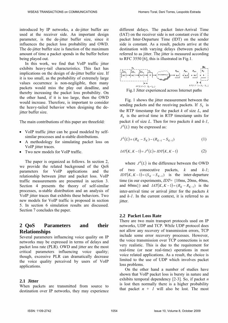
different delays. The packet Inter-Arrival Time (IAT) on the receiver side is not constant even if the packet Inter-Departure Time (IDT) on the sender side is constant. As a result, packets arrive at the destination with varying delays (between packets) referred to as jitter. The jitter is measured according to RFC 3550 [6], this is illustrated in Fig.1.

Fig.1 Jitter experienced across Internet paths

Fig. 1 shows the jitter measurement between the

sending packets and the receiving packets. If kS is the RTP timestamp for the packet k of size L, and

kR is the arrival time in RTP timestamp units for packet k of size L. Then for two packets k and k-1,

( )LJ k may be expressed as: ( ) )()( 11 −− −−−= KKKK

k SRSRLJ (1)

( ) ( ) ( )1,1, −+=− KKIDTLJKKIAT k (2)

where ( )LJ k is the difference between the OWD of two consecutive packets, k and k-1;

( ) )(1, 1−−=− KK SSKKIDT is the inter-departure time (in our experiments, IDT= {10ms, 20ms, 40ms, and 60ms}) and ( ) )(1, 1−−=− KK RRKKIAT is the inter-arrival time or arrival jitter for the packets k and k-1. In the current context, it is referred to as jitter. 2.2 Packet Loss Rate There are two main transport protocols used on IP networks, UDP and TCP. While UDP protocol does not allow any recovery of transmission errors, TCP include some error recovery processes. However, the voice transmission over TCP connections is not very realistic. This is due to the requirement for real-time (or near real-time) operations in most voice related applications. As a result, the choice is limited to the use of UDP which involves packet loss problems.

On the other hand a number of studies have shown that VoIP packet loss is bursty in nature and exhibits temporal dependency [2-3]. So, if packet n is lost then normally there is a higher probability that packet n + 1 will also be lost. The most



generalized model to capture temporal dependency, is a finite Markov chain [4]. Because of its simplicity and effectiveness, a two state Markov model or Gilbert model is often used to simulate packet loss patterns. Fig. 2 shows the state diagram of this 2-state Markov model.

Fig. 2 Two-state Markov model

In this model, one of the states (state 1)

represents a packet loss and the other state (state 0) represents the case where packets are correctly transmitted or found. The transition probabilities in this model, as shown in Fig. 2, are represented by p and q. In other words, p is the probability of going from state 0 to state 1, and q is the probability of going from state 1 to state 0.

The probability that n consecutive packets are lost is given by ( ) 11 −− nqp . If ( ) pq >−1 , then the probability of losing a packet is greater after having already a lost packet than after having successfully a received one. This is generally the case in data transmission on the Internet where packet losses occur as bursts.

Different values of p and q representing different packet loss and network conditions that can occur on the Internet.

In equation (3), b corresponds to the average burst length.

qb

qppPLR 1

=+

= (3)

2.3 Packet Loss Effects on the VoIP Jitter The successive voice packets are transmitted at a constant rate, where the voice data rate is equal to the packetization interval or voice data length (i.e.

10ms, 20ms, 40ms and 60ms). However, when voice packets are transported over IP networks, they may experience delay variations and packet loss. On the other hand, in the measurements it is observed that packet loss has serious implications on the VoIP jitter.

0

60

120

180

240

300

24000 25000 26000 27000 28000 29000 30000 31000 32000

Time

Jitte

r (m

s)If there is no packet lost If one packet is lostIf two consecutive packets are lost If three consecutive packets are lost

Fig. 3 Packet loss effects on VoIP jitter

The equation (2) describes the VoIP jitter for the packets k and k-1. From this equation can be found a relationship between jitter and packet loss. If the packet k-1 is lost,

( ) ( ) ( )IDTLJKKIAT k 22, +=− , therefore, if n consecutive packets are lost, then:

( ) ( ) ( )( )IDTnLJnKKIAT k 11, ++=−− (4) were ( )LJ k is the difference between the OWD

of two consecutive packets that arrive in the receiver side. This behavior is illustrated in Fig. 3, where a voice data length equal to 60ms is used.

Therefore, the equation (4) describes the packet loss effects on the VoIP jitter. 3 Measurements Voice over IP demands strict quality of service levels. However, the current Internet only offers best-effort services due to its shared nature and cannot guarantee the required QoS. VoIP is susceptible to suffer impairments, which result in voice quality degradation. Therefore, it is necessary, to monitor voice quality constantly, and to cope with possible voice quality degradation. To do this, active measurement and passive measurement can be considered. In the active measurements, VoIP traffic was generated by establishing test calls with the Alliance FXS VoIP application [7]. Alliance FXS is a system



developed at CTS CINVESTAV GDL composed by a PCI board and application software that allows connecting regular telephone sets to the IP network. Each board allows having four extensions. Multiple Alliance FXS boards can be installed in a single PC, as shown in Figure 4.

Fig. 4 Alliance FXS

The main characteristics of Alliance FXS are the following: • PCI board (26.2cm x 12.0cm) • 4 RJ-11 ports for analog telephone sets • Each port supports lines up to 4 kilometers long • H.323 architecture [8] • G.711-A Law [9] and G.729 [10] hardware

compression • ITU-T G.165 and G.168 echo canceller on the

four ports • DTMF detection compliant with ITU-T Q.24,

Bellcore GR-30 CORE and BAPT 223 ZV5 • Adjustable gain in reception from -10 dB to +2

dB • Adjustable gain in transmission from +10 dB to -

5 dB • Ring signal compatible with ANSI/EIA/TIA-

464-A-1989 • ITU-T V.23 and Bell 202 Caller Id generation In the passive measurements, we realized the capture of VoIP traffic using Wireshark [11] to obtain a set of data traces. The subject of these measurements is to gather traffic patterns of RTP packets such as: Jitter, sequence number of the packets and post-processing analysis. Table 1 Relationship between the voice data length

and samples size Data Traces

Length (samples) Voice Data Length (ms)

Voice Data Length (Bytes)

G.711 G.729 360,000 10 80 10

180,000 20 160 20

90,000 40 320 40

60,000 60 480 60

For the collected data sets (Table 2), we used the parameters showed in Table 1. In this table it is

observed the relationship between the voice data lengths and the samples size for one hour of measurement. The voice codec G.711 and G.729 with voice data length of 10, 20, 40 and 60 ms are used. The test scenario where the VoIP traffic was measured consists of two different LANs (different ISPs), interconnected by the Internet backbone [12]: • LAN “A” - Local Cable ISP network (Link

Speed-3MB)

• LAN “B” - CINVESTAV GDL network (Link Speed-2MB)

Figure 5 shows a typical H.323 architecture [8], composed of two zones interconnected via Internet. Each zone consists of a single H.323 gatekeeper (GK) [13] which acts as the administrator of the zone [14], and a number of H.323 terminal endpoints (TEs), interconnected via a LAN. The zone “A” is composed of the endpoints A1, A2, A3, and A4, this zone is administrated for the gatekeeper “A”. In this zone, the network protocol analyzer Wireshark was installed for collecting the data traces. On the other hand the zone “B” is composed of the endpoints B1, B2, B3 and B4, the gatekeeper “B” and a workstation where is monitoring the routes that follows the test calls. In order to make calls between any endpoints, each endpoint has installed an Alliance FXS PCI card and a conventional cord phone.

Set A1/B1 A2/B2 A3/B3 A4/B4

Set 1 G.711-10ms G.711-20ms G.711-40ms G.711-60ms Set 2 G.729-10ms G.729-20ms G.729-40ms G.729-60ms Set 3 G.711-10ms G.711-20ms G.729-10ms G.729-20ms Set 4 G.711-40ms G.711-60ms G.729-40ms G.729-60ms

Fig. 5 Alliance FXS The measurements corresponding to the data traces used in this work are shown in Table 2. In this table, can be seen that VoIP jitter traces were collected in the following way:



• Four simultaneous test calls were established between A1/B1, A2/B2, A3/B3 and A4/B4 endpoints, see Figure 5.

• The measurement periods were 60 minutes for each test call (call duration time)

• Four different configuration sets for the endpoints were used, see Figure 5.

• For each measurement period (an hour), four jitter and sequence number data traces were obtained

Table 2 Description of used VoIP jitter traces

Data Set

Measurement Periods

Total Number of Traces

CODEC-Voice Data Length(ms)

Set 1 Sep/07/2007, 10:00am-04:00pm

24 Jitter Traces

G.711-10ms G.711-20ms G.711-40ms G.711-60ms

Set 2 Sep/10/2007, 10:00am-04:00pm

24 Jitter Traces

G.729-10ms G.729-20ms G.729-40ms G.729-60ms

Set 3 Sep/11/2007, 10:00am-04:00pm

24 Jitter Traces

G.711-10ms G.711-20ms G.729-10ms G.729-20ms

Set 4 Sep/12/2007, 10:00am-04:00pm

24 Jitter Traces

G.711-40ms G.711-60ms G.729-40ms G.729-60ms

4 Self-Similar and Heavy-Tail Analysis 4.1 Mathematical Background Self-Similar Processes: Traffic processes are said to be self-similar if certain property of the processes is preserved with respect to scaling in space and/or time [15-18]. Considering a discrete time stochastic process or time series ( )Ν∈= tXX tt ; with mean Xμ , variance

2Xσ , autocorrelation function ( )kr and

autocovariance function (ACV) ( )kγ , 0≥k ; where tX can be interpreted as the traffic volume at time

instance t , or Jitter. To formulate the phenomenon of scale invariance, the aggregated process is defined as

( )Ν∈= kXX mk

mk ;)()( (5)

where )(mkX is obtained by averaging the original

series tX over non-overlapping blocks of size m , and each term )(m

kX is given by

( )

( ),...3,2,1;1

11

== ∑+−=

kXm

Xkm

mkii

mk (6)

Here, tX is self-similar ( )ssH − with self-similarity parameter H , i.e. Hurst Parameter ( )10 << H if:

tH

dm

k XmX 1)( −= (7)

where d= denotes equality in distribution.

Let ( )kmγ denote the autocovariance function of )(m

kX . The process tX is called exactly second order self-similar with Hurst parameter H if

( ) ( ) ( )( )HHHX kkkk 2222

1212

−+−+= σγ (8)

for all 1≥k . tX is called asymptotically second-order self-similar if

( ) ( ) ( )( )HHHXm

mkkkk 222

2121

2lim −+−+=

∞→

σγ (9)

Equations (8) and (9), express the fact than tX and

)(1 mk

H Xm − are required to have exactly or asymptotically the same second-order structure. From equation (7) it follows that

( ) 222)(var −⋅= HX

mk mX σ (10)

Let ( ) ( ) 2

Xkkr σγ= denote the autocorrelation function. For 10 << H

( ) ( ) 2212~ −− HkHHkr ∞→k . (11)

In particular, if 121

<< H , ( )kr asymptotically

behaves as η−ck for 10 <<η , where 0>c is a

constant, H22 −=η and ( ) ∞=∑∞

−∞=k

kr . That is, the

autocorrelation function decays slowly, which is the essential property that causes it to diverge. When ( )kr obeys a power-law, the corresponding

stationary process tX is called long range



dependent (LRD). tX is short range dependent

(SRD) if the sum ( ) ∞<∑∞

−∞=k

kr does not diverge.

Following are some simple facts regarding the value of H and its impact on ( )kγ .

• ( )⎩⎨⎧

≠=

=0,00,1

kk

kγ for 5.0=H . This is the well-

known property of white Gaussian noise. • • ( ) 01 <γ for 5.00 << H . • • ( ) 01 >γ for 15.0 << H . Properties 2 and 3 are often termed antipersistent and persistent correlations, respectively. Distribution with ‘Heavy-Tail’ (DHT): A random variable (r.v.) X has a ‘heavy-tail’ distribution if:

[ ] 20;;1~ <<∞→> αα

xx

xXP (12)

where α is called the ‘tail’ index. Note that, heavy-tail distribution decays slower than exponential function. It is known that a heavy-tail r. v. has infinite variance, also when 10 ≤< α its mean is infinite [15]. α-stable Distribution: A r. v. X is said to have an α-stable distribution if there are parameters 20 ≤< α ,

2≥a , 11 ≤≤− β , and ℜ∈b , such that its characteristic function has the following form [19]:

( ) [ ] ( ) ( )[ ]{ }αωθωβωωω αω ,sgn1exp jajbeE Xj −−==Φ (13) where:

( )⎪⎪⎩

⎪⎪⎨

⎧

=−

≠⎟⎠⎞

⎜⎝⎛

=1;ln2

1;2

tan,

αωπ

ααπ

αωθ (14)

In equation (6), α is the stability index; β , the skewness parameter; a , the scaling parameter and b , the shift parameter. 4.2 Self-Similar Analysis For the H parameter estimation at seven aggregation levels, ( }128,64,32,16,8,4,2{=m ) six methods,

implemented in SelQos [20-22], were used. They are: R/S statistic (R/S), Absolute Moment (AM), Variance Method (VAR), Modified Allan Variance (MAVAR), Periodogram (PER), y Local Whittle (WHI). Figure 6 shows the Hurst Parameter of the Jitter traces as a function of the aggregation level. We observe the phenomenon of scale invariance at different time scales. These results indicate that the analyzed VoIP Jitter traces have self-similar characteristics.

0

0.1

0.2

0.3

0.4

0.5

0.6

0.7

0.8

1 2 4 8 16 32 64 128Agg Lvl

Hur

st P

aram

eter

(H)

G.711_10ms G.711_20ms G.711_40ms G.711_60ms G.729_10msG.729_20ms G.729_40ms G.729_60ms

Fig. 6 Hurst parameter for different aggregation levels

The autocovariance function of representative VoIP Jitter traces is illustrates in Figure 7.

Fig. 7 Autocovariance function for VoIP Jitter traces ¡Error! No se encuentra el origen de la referencia. shows a comparison between the autocovariance function of a measured data trace with 4223.0=H and the theoretical autocovariance function defined by equation (8). It can be observed that the autocovariance function of the measured data trace behaves similarly to the ideal model. This indicates that the VoIP Jitter traces exhibit memoryless property or SRD.



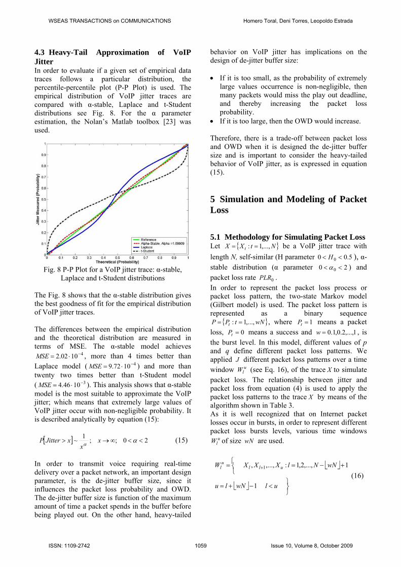
4.3 Heavy-Tail Approximation of VoIP Jitter In order to evaluate if a given set of empirical data traces follows a particular distribution, the percentile-percentile plot (P-P Plot) is used. The empirical distribution of VoIP jitter traces are compared with α-stable, Laplace and t-Student distributions see Fig. 8. For the α parameter estimation, the Nolan’s Matlab toolbox [23] was used.

Fig. 8 P-P Plot for a VoIP jitter trace: α-stable,

Laplace and t-Student distributions The Fig. 8 shows that the α-stable distribution gives the best goodness of fit for the empirical distribution of VoIP jitter traces. The differences between the empirical distribution and the theoretical distribution are measured in terms of MSE. The α-stable model achieves

41002.2 −⋅=MSE , more than 4 times better than Laplace model ( 41072.9 −⋅=MSE ) and more than twenty two times better than t-Student model ( 31046.4 −⋅=MSE ). This analysis shows that α-stable model is the most suitable to approximate the VoIP jitter; which means that extremely large values of VoIP jitter occur with non-negligible probability. It is described analytically by equation (15):

[ ] 20;;1~ <<∞→> αα

xx

xJitterP (15)

In order to transmit voice requiring real-time delivery over a packet network, an important design parameter, is the de-jitter buffer size, since it influences the packet loss probability and OWD. The de-jitter buffer size is function of the maximum amount of time a packet spends in the buffer before being played out. On the other hand, heavy-tailed

behavior on VoIP jitter has implications on the design of de-jitter buffer size: • If it is too small, as the probability of extremely

large values occurrence is non-negligible, then many packets would miss the play out deadline, and thereby increasing the packet loss probability.

• If it is too large, then the OWD would increase. Therefore, there is a trade-off between packet loss and OWD when it is designed the de-jitter buffer size and is important to consider the heavy-tailed behavior of VoIP jitter, as is expressed in equation (15). 5 Simulation and Modeling of Packet Loss 5.1 Methodology for Simulating Packet Loss Let { }NtXX t ,...,1: == be a VoIP jitter trace with length N, self-similar (H parameter 5.00 0 << H ), α-stable distribution (α parameter 20 0 << α ) and packet loss rate 0PLR . In order to represent the packet loss process or packet loss pattern, the two-state Markov model (Gilbert model) is used. The packet loss pattern is represented as a binary sequence

{ }wNtPP t ,...,1: == , where 1=tP means a packet loss, 0=tP means a success and 1,...,2.0,1.0=w , is the burst level. In this model, different values of p and q define different packet loss patterns. We applied J different packet loss patterns over a time window u

lW (see Eq. 16), of the trace X to simulate packet loss. The relationship between jitter and packet loss from equation (4) is used to apply the packet loss patterns to the trace X by means of the algorithm shown in Table 3. As it is well recognized that on Internet packet losses occur in bursts, in order to represent different packet loss bursts levels, various time windows

ulW of size wN are used.

⎣ ⎦

⎣ ⎦⎭⎬⎫<−+=

⎩⎨⎧ +−== +

ulwNlu

wNNlXXXW ullu

l

1

1,...,2,1:,...,, 1

(16)



where lX and uX are the l-th and u-th element of time series X and represent the window beginning and ending, respectively.

Table 3 Algorithm for simulating packet loss: A) Generating packet loss pattern B) Applying packet loss pattern

A) B)

FOR 11 −= lton

0][ =nP

END FOR

FOR utoln =

IF (packet was lost)

1][ =nP

ELSE

0][ =nP

END IF

END FOR

FOR Ntoun 1+=

0][ =nP

END FOR

FOR Nton 2=

IF ( 1][ =nP )

]1[][][ −+= nXnXnX

END IF

END FOR

1=i

FOR Nton 2=

IF ( 1][ ≠nP )

]1[][ˆ −= nXiX

1+= ii

END IF

END FOR

By means of the above algorithm the new time series jX are obtained, where 1,...2,1,0 −= Jj . For each jX the PLR, H parameter and the α parameter were calculated, and the functions ( )jjw HPLRf , and

( )jjw PLRf α, was generated. 5.2 Proposed Models From our simulations, we found that the relationship between H parameter and α parameter with the PLR can be modeled by a power-law function, characterized by three fitted parameters, as following: • Relationship between H and PLR:

( ) 110ˆ b

M PLRaHH += (17)

5.0ˆ0 0 << H , 01 >a and 01 >b • Relationship between α and PLR:

( ) 220ˆ b

M PLRa+=αα (18)

2ˆ0 0 <<α , 02 <a and 02 >b Where MH and Mα are the H parameter and α parameter of the found models, respectively, 0H and 0α are the H parameter and α parameter when

0=PLR , respectively. 6 Simulation Results In this section, applying the methodology proposed in section 5, simulation results are presented. The simulations are accomplished over VoIP jitter traces corresponding to Table 2. 6.1 Relationship between H and PLR Figure 9 illustrates the relationships between packet loss rate and Hurst parameter. The functions family

( )jjw HPLRf , , is result to apply " J " packet loss patterns to time series tX over a time window “w”. The time series tX represents a VoIP Jitter trace of the data sets described in Table 2. In this figure, each point of the function ( )jjw HPLRf , represents a

new time series jX . The function ( )Mjw HPLRf , is the function of the found model.

0.3

0.4

0.5

0.6

0.7

0.8

0.9

1

0 0.5 1 1.5 2 2.5 3 3.5 4

Packet Loss Rate (%)

Hur

st P

aram

eter

(H-V

AR

)

w=0.1 w=0.2 w=0.3 w=0.4 w=0.5 w=0.6

w=0.7 w=0.8 w=0.9 w=1.0 REAL Fig. 9 Relationship between PLR and H parameter:

( )jjw HPLRf , vs. ( )Mj HPLRfw ,

The difference between the function corresponding to measurements results ( )jjw HPLRf , and the function corresponding to the found model

( )Mjw HPLRf , , was quantified in terms of mean square error:



( ) ( )[ ]2,,1jjwMjw

PLR

PLRMinMaxHPLRfHPLRf

PLRPLRMSE

Max

Min

−−

= ∫

Ii ,...2,1= Table 4 shows the fitted parameters and MSE

between ( )Mjw HPLRf , and ( )jjw HPLRf , corresponding for each time window.

Table 4 Fitted parameters for Figure 9

( )jjw HPLRf , 0H a b MSE

w=0.1 0.0428 0.6457 0.2623 0.0144

w=0.2 0.0428 0.5963 0.2548 0.0032

w=0.3 0.0428 0.5673 0.2453 0.0004

w=0.4 0.0428 0.5431 0.2390 0.0003

w=0.5 0.0428 0.5213 0.2328 0.0019

w=0.6 0.0428 0.5069 0.2160 0.0047

w=0.7 0.0428 0.4901 0.2001 0.0091

w=0.8 0.0428 0.4724 0.1789 0.0155

w=0.9 0.1738 0.3194 0.2010 0.0261

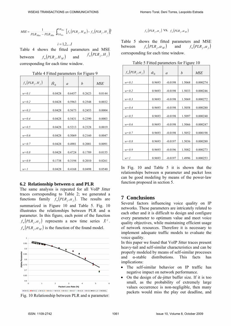
w=1 0.0428 0.4168 0.0498 0.0540 6.2 Relationship between α and PLR The same analysis is repeated for all VoIP Jitter traces corresponding to Table 2; we generated a functions family ( )jjw PLRf α, . The results are summarized in Figure 10 and Table 5. Fig. 10 illustrates the relationships between PLR and α parameter. In this figure, each point of the function

( )jjw PLRf α, represents a new time series jX . ( )Mjw PLRf α, is the function of the found model.

0.6

0.65

0.7

0.75

0.8

0.85

0.9

0.95

1

0 1 2 3 4 5 6

Packet Loss Rate (%)

Alp

ha P

aram

eter

W=0.1 W=0.2 W=0.3 W=0.4 W=0.5 W=0.6 W=0.7 W=0.8 W=0.9 W=1.0 MODEL Fig. 10 Relationship between PLR and α parameter:

( )jjw PLRf α, vs. ( )Mjw PLRf α, Table 5 shows the fitted parameters and MSE between ( )Mjw PLRf α, and ( )jjw PLRf α, corresponding for each time window.

Table 5 Fitted parameters for Figure 10

( )jjw PLRf α, 0α a b MSE

w=0.1 0.9693 -0.0198 1.5068 0.000274

w=0.2 0.9693 -0.0198 1.5033 0.000246

w=0.3 0.9693 -0.0198 1.5069 0.000272

w=0.4 0.9693 -0.0198 1.5058 0.000280

w=0.5 0.9693 -0.0198 1.5097 0.000240

w=0.6 0.9693 -0.0198 1.5066 0.000247

w=0.7 0.9693 -0.0198 1.5052 0.000198

w=0.8 0.9693 -0.0197 1.5036 0.000280

w=0.9 0.9693 -0.0196 1.5082 0.000273

w=1 0.9693 -0.0197 1.4996 0.000253 In Fig. 10 and Table 5 it is shown that the relationships between α parameter and packet loss can be good modeling by means of the power-law function proposed in section 5. 7 Conclusions Several factors influencing voice quality on IP networks. These parameters are intricately related to each other and it is difficult to design and configure every parameter to optimum value and meet voice quality objectives, while maintaining efficient usage of network resources. Therefore it is necessary to implement adequate traffic models to evaluate the voice quality. In this paper we found that VoIP Jitter traces present heavy-tail and self-similar characteristics and can be properly modeled by means of self-similar processes and α-stable distributions. This facts has implications: • The self-similar behavior on IP traffic has

negative impact on network performance. • On the design of de-jitter buffer size. If it is too

small, as the probability of extremely large values occurrence is non-negligible, then many packets would miss the play out deadline, and



thereby increasing the packet loss probability. On the other hand, if it is too large, then the OWD would increase.

Therefore, it is important to consider models that capture these behaviors for the design and performance analysis of computer networks and when designing the de-jitter buffer size. On the other hand, we have presented a methodology for simulating packet loss on VoIP jitter traces. In this methodology the packet loss effects on VoIP jitter and the two state Markov model are used. Based on the above methodology, we have proposed a new model for VoIP traffic. The new models are based on voice traffic measurement and allowed to relate three important parameters, the H parameter, the α parameter and PLR. We found that H parameter and α parameter is related with the PLR by a power-law with three fitted parameters. Simulation results show the effectiveness of our model in terms of MSE. ACKNOWLEDGMENTS The authors gratefully acknowledge the support of CONACYT by means of the scholarship number 44459. References: [1] T. Palade, and E. Puschita, Requirements for a

New Resource Reservation Model in Hybrid Access Wireless Network, WSEAS Transactions on Communications, Volume 7, Issue 3, (2008) 144-151.

[2] M. Yajnik, S. Moon, J. Kursoe and D. Towsley, Measurement and Modelling of the Temporal Dependence in Packet Loss, Proc. IEEE INFOCOM’99, New York, NY, pp. 345–352, March 1999.

[3] R. Singh and A. Ortega, Modeling of Temporal Dependence in Packet Loss Using Universal Modeling Concepts, Proc. 12th Packet Video Workshop, Pittsburgh, PA, Apr. 2002.

[4] ITU-T Recommendation G.1050, Network Model for Evaluating Multimedia Transmission Performance over Internet Protocol, International Telecommunications Union, Geneva, Switzerland, 2005.

[5] R. Dobrescu, D. Hossu, S. Mocanu and M. Nicolae, New algorithms for QoS performance improvement in high speed networks, WSEAS Transactions on Communications, Volume 7, Issue 12, (2008) 1192-1201.

[6] RFC 3550, RTP: A Transport Protocol for Real-Time Applications, Internet Engineering Task Force, 2003.

[7] Advanced Information CTS (Centro de Tecnología de Semiconductores) Property, Alliance FXO/FXS/E1 VoIP System, www.cts-design.com.

[8] ITU-T Recommendation H.323, Packet-Based Multimedia Communications Systems, International Telecommunications Union, Geneva, Switzerland, 2007.

[9] ITU-T Recommendation G.711, Pulse Code Modulation (PCM) of Voice Frequencies, International Telecommunications Union, Geneva, Switzerland, 1993.

[10] ITU-T Recommendation G.729, Coding of speech at 8 kbit/s using Conjugate-Structure Algebraic-Code-Excited Linear-Prediction (CS-ACELP), International Telecommunications Union, Geneva, Switzerland, 2008.

[11] Wireshark: A Network Protocol Analyzer, http://www.wireshark.org/.

[12] H. Toral, D. Torres, C. Hernandez and L. Estrada, Self-Similarity, Packet Loss, Jitter, and Packet Size: Empirical Relationships for VoIP, Proceedings IEEE CONIELECOMP, Puebla, Mexico, pp. 11-16, 2008.

[13] Gatekeeper: OpenH323 Gatekeeper - The GNU Gatekeeper, http://www.gnugk.org/.

[14] A. Maraj, and I. Imeri, WiMAX integration in NGN network, architecture, protocols and Services, WSEAS Transactions on Communications, Volume 8, Issue 7, (2009) 708-717.

[15] O. I. Sheluhin, S. M. Smolskiy, and A. V. Osin, Self-Similar Processes in Telecommunications, JohnWiley & Sons, Ltd, chapters 1 and 3, 2007.

[16] T. Janevski, Traffic Analysis and Design of Wireless IP Networks, Artech House Mobile Communications Series, 2003, chapter 2, 3, 4, 5.

[17] W.E. Leland, M.S. Taqqu, W. Willinger, and D.V. Wilson, On the Self-Similar Nature of Ethernet Traffic (Extended Version), IEEE/ACM Transactions on Networking, Volume 2, issue 1, (1994) 1-15.

[18] K. Park and W. Willinger, Self-Similar Network Traffic and Performance Evaluation, John Wiley & Sons, Inc., 2000, chapter 1.

[19] A. Karasaridis, and D. Hatzinakos, Network Heavy Traffic Modeling Using α-Stable Self-Similar Processes, IEEE Transactions on Communications, Vol. 49, No. 7, pp. 1203-1214, 2001.



[20] J. Ramírez and D. Torres, A Tool for Analysis of Internet Metrics, Mexico, D.F., Proceedings CIE, (2005) 60-63.

[21] J. Ramírez and D. Torres, Development of a tool for basic analysis of Internet self-similar traffic, Master’s Thesis (Thesis in Spanish), CINVESTAV del IPN Unidad Guadalajara, (2005).

[22] O. Rincon, y D. Torres, Advance software for Internet metrics analysis with applications to time series, Master’s Thesis (Thesis in Spanish), CINVESTAV del IPN Unidad Guadalajara, (2006).

[23] J. P. Nolan, Stable MathLink Package, www.robustanalysis.com.



Simulation and Modeling of Packet Loss on VoIP …€¦ · Simulation and Modeling of Packet Loss...

Documents

Transcript of Simulation and Modeling of Packet Loss on VoIP …€¦ · Simulation and Modeling of Packet Loss...