Thèse de doctorat - Centro de Matemáticalessa/resource/these.pdfcrecimiento de volumen de dichas...

UniversitéPierre et MarieCurie

Universidad dela República

École Doctorale Paris Centre et PEDECIBA

Thèse de doctoratDiscipline : Mathématiques

présentée par

Pablo Lessa

Brownian motion on stationary random manifolds

dirigée par François Ledrappier et Matilde Martínez

Soutenue le 18 mars 2014 devant le jury composé de :

M. Jesús Álvarez U. de Santiago de Compostela rapporteurM. Yves Coudene Université de Bretagne Occidentale examinateurM. Gilles Courtois Université Paris 6 examinateurM. Vadim Kaimanovich Université d’Ottawa rapporteurM. Raphaël Krikorian Université Paris 6 examinateurM. François Ledrappier Université Paris 6 directeurMme. Matilde Martínez Universidad de la República directeur

3

Institut de Mathématiques de Jussieu175, rue du chevaleret75 013 Paris

École doctorale Paris centre Case 1884 place Jussieu75 252 Paris cedex 05

Centro de MatemáticaFacultad de CienciasIguá 422511400 Montevideo

Dedicada a Marcela por los mejores años de mi vida.

Serendipity: The occurrence anddevelopment of events by chance in ahappy or beneficial way.

Acknowledgements

François Ledrappier and Matilde Martinez have been the perfect advisors, simultaneouslychallenging and enabling me to do better mathematics, I thank them deeply.

I also owe a lot to Martín Sambarino who among other things introduced me to Françoisand arranged for me to be coadvised by Matilde.

Fernando Alcalde invited me to give my first ever talk and also handed me a copyof Benjamini and Curien’s work on stationary random graphs. It turned out to be a keypiece for this work and I would like to thank him especially for bringing it to my attention.

I learned many interesting things thanks to conversations with Bertrand Deroin, Chris-tian Bonatti, Sébastien Álvarez, Liviu Nicolaescu, Renato Bettiol, Karsten Grove, MiguelPaternain and Rafael Potrie.

I would like to thank Jairo Bochi and Samuel Senti for inviting me to speak at Semi-nario Edaí, Barbara Shapira for inviting me to the workshop on non-positive curvature atLuminy, and Alberto Verjovski for several interesting conversations.

I have been lucky to have had ideal rapporteurs in Jesús Álvarez Lopez and VadimKaimanovich, I thank them for their comments and corrections.

Funding for my travels was provided by IFUM and CSIC, I also benefited from a CSICscholarship, and have been partially supported by ANII as an SNI candidate researcher.I’m also grateful to the University of Notre Dame for having me as a visitor on severaloccasions.

Special thanks go to my friends in Rio: Guarino, Vivis, Luciano and Yuri. To theUruguayans in Paris especially Andrés Sambarino and Matías Carrasco. To Safia andPatrice for their hospitality. To the fellow students at LPMA especially Cyril, Guil-laume, Bastien, Nelo, Xan, Alexandre, and Nikos. To the fluid dynamics and lunch-coffee-chocolate group at Notre Dame, Liviu, Misha, François, Roxana, Nero, and Richard. Tothe young guys (and gal) at Notre Dame, Quinn, James, Ryan, Renato, and Amy. To thegroup back in Montevideo especially Gordo, Diego, Leva, Juliana, Rata and Frodo. Tomy parents Enrique and María Paz, my sister Carolina, and my fiancée Marcela.

Abstract

Brownian motion on stationary random manifolds

Abstract

We introduce the concept of a stationary random manifold with the objective of treatingin a unified way results about manifolds with transitive isometry group, manifolds with acompact quotient, and generic leaves of compact foliations. We prove inequalities relatinglinear drift and entropy of Brownian motion with the volume growth of such manifolds,generalizing previous work by Avez, Kaimanovich, and Ledrappier among others. In thesecond part we prove that the leaf function of a compact foliation is semicontinuous,obtaining as corollaries Reeb’s local stability theorem, part of Epstein’s local structuretheorem for foliations by compact leaves, and a continuity theorem of Álvarez and Candel.

Keywords

Ergodic theory, Random manifolds, Brownian motion, Entropy, Liouville property.

Mouvement brownien sur les variétés aléatoiresstationnaires

Résumé

On introduit le concept d’une variété aléatoire stationnaire avec l’objectif de traiter defaçon unifiée les résultats sur les variétés avec un group d’isométries transitif, les variétésavec quotient compact, et les feuilles génériques d’un feuilletage compact. On démontredes inégalités entre la vitesse de fuite, l’entropie du mouvement brownien et la croissancede volume de la variété aléatoire, en généralisant des résultats d’Avez, Kaimanovich, etLedrappier. Dans la deuxième partie on démontre que la fonction feuille d’un feuilletagecompact est semicontinue, en obtenant comme conséquences le théorème de stabilité localde Reeb, une partie du théorème de structure local pour les feuilletages à feuilles compactesd’Epstein, et un théorème de continuité d’Álvarez et Candel.

8

Mots-clefs

Théorie ergodique, Variétés aléatoires, Mouvement brownien, Entropie, Propriétés de Liou-ville.

Movimiento Browniano en variedades aleatoriasestacionarias

ResumenIntroducimos el concepto de variedad aleatoria estacionaria con el fin de probar en for-ma unificada resultados sobre variedades con grupo de isometría transitivo, variedadescon cociente compacto, y hojas genéricas de foliaciones compactas. Probamos desigualda-des relacionando la velocidad de escape del movimiento Browniano con la entropía y elcrecimiento de volumen de dichas variedades generalizando trabajos anteriores de Avez,Kaimanovich, y Ledrappier entre otros. En la segunda parte mostramos que la funciónhoja de una foliación compacta es semicontinua, obteniendo como corolarios el teorema deestabilidad local de Reeb, parte del teorema de estructura local de Epstein para foliacionespor hojas compactas, y el teorema de continuidad de Álvarez y Candel.

Palabras claves

Teoría ergódica, Variedades aleatorias, Movimiento Browniano, Entropía, Propiedad deLiouville.

Contents

Introduction 11

I Ergodic theory of stationary random manifolds 13

1 Liouville properties and Zero-one laws on Riemannian manifolds 151.1 Brownian motion and the backward heat equation . . . . . . . . . . . . . . 161.2 A bounded backward heat solution . . . . . . . . . . . . . . . . . . . . . . . 231.3 Steadyness of Brownian motion . . . . . . . . . . . . . . . . . . . . . . . . . 251.4 Mutual information . . . . . . . . . . . . . . . . . . . . . . . . . . . . . . . . 28

2 Entropy of stationary random manifolds 332.1 The Gromov space and harmonic measures . . . . . . . . . . . . . . . . . . 352.2 Asymptotics of random manifolds . . . . . . . . . . . . . . . . . . . . . . . . 44

3 Brownian motion on stationary random manifolds. 553.1 Brownian motion on stationary random manifolds . . . . . . . . . . . . . . 563.2 Busemann functions and linear drift . . . . . . . . . . . . . . . . . . . . . . 643.3 Entropy of reversed Brownian motion . . . . . . . . . . . . . . . . . . . . . 67

II Gromov-Hausdorff convergence of leaves of compact foliations 75

4 The leaf function of compact foliations 774.1 Introduction . . . . . . . . . . . . . . . . . . . . . . . . . . . . . . . . . . . . 774.2 Examples of leaf functions . . . . . . . . . . . . . . . . . . . . . . . . . . . . 784.3 Regularity of leaf functions . . . . . . . . . . . . . . . . . . . . . . . . . . . 824.4 Uniformly bounded geometry . . . . . . . . . . . . . . . . . . . . . . . . . . 864.5 Smooth precompactness . . . . . . . . . . . . . . . . . . . . . . . . . . . . . 894.6 Curvature and injectivity radius . . . . . . . . . . . . . . . . . . . . . . . . 944.7 Smooth convergence and tensor norms . . . . . . . . . . . . . . . . . . . . . 964.8 Bounded geometry of leaves . . . . . . . . . . . . . . . . . . . . . . . . . . . 994.9 Covering spaces and holonomy . . . . . . . . . . . . . . . . . . . . . . . . . 1004.10 Convergence of leafwise functions . . . . . . . . . . . . . . . . . . . . . . . . 103

Bibliography 107

Introduction

This thesis has two parts. In the first we are concerned with harmonic measures offoliations, the entropy theory of Riemannian manifolds, Liouville properties, and howthey relate to the behavior of Brownian motion. The main influence for this part of ourwork are the two very rich papers of Kaimanovich, [Kaı86] and [Kaı88]. By analogy withthe, by then, well established theory of entropy for random walks on discrete groups (see[KV83]), Kaimanovich defined an entropy for Riemannian manifolds and outlined how thisentropy would relate to the Liouville properties, algebraic properties of the fundamentalgroup of the manifold, and volume growth among other things. The main idea is thatthe Riemannian metric on the manifold must have some sort of recurrence in order forthis statistical approach to work. The three main cases where one suspects that thisrecurrence condition is satisfied are: manifolds with transitive isometry group, manifoldswith a compact quotient, and generic leaves of compact foliations.

The entropy theory of discrete groups has seen its results successively generalized tomore general types of graphs then just Cayley graphs. So for example in [KW02] thetheory is worked out for graphs whose isometry group is transitive. Benjamini and Curien[BC12] have introduced the concept of a stationary random graph which simultaneouslygeneralizes and includes the case of Cayley graphs and graphs with transitive isometry.Following their lead we introduce the concept of a stationary random manifold, which isa rooted random manifold whose distribution is invariant under re-rooting by Brownianmotion, and develop the basic theory of entropy for them. This concept allows for unifiedproofs of results about manifolds with transitive isometry group, compact quotient, orgeneric leaves of compact foliations.

The first part of the thesis is divided into three chapters. In the first we deal withresults about a single manifold, roughly the relationship between the Liouville property andthe behavior of Brownian motion on the manifold. In the second we introduce stationaryrandom manifolds and three invariants for them: Kaimanovich entropy, linear drift (themean rate of displacement of Brownian motion from the basepoint), and volume growth(which measures the exponential growth rate of the volume of balls as a function of theirradii). The main results are that entropy exists, is non-negative, and is zero if and onlyif the manifold is almost surely Liouville; and the basic inequalities relating the threeasymptotic quantities which are

12`(M)2 ≤ h(M) ≤ `(M)v(M)

where `(M), h(M) and v(M) are the drift, entropy and volume growth respectively. Theseinequalities have several interesting consequences which had been established indepen-dently before. The third chapter deals with Brownian motion on stationary randommanifolds and can be seen as a more detailed look at the results in the second chap-ter (in particular we improve the lower bound for entropy above, following the results of

12 Introduction

Kaimanovich and Ledrappier for manifolds with compact quotient [Kaı86, Theorem 10],[Led10, Theorem A]).

In the second part of the thesis we prove geometric results about how the leaves ofa compact foliation vary from point to point. The only thing we had needed to knowabout compact foliations in the first part of the thesis was that the leaf of a randompoint whose distribution is harmonic in the sense of Garnett [Gar83] is an example of astationary random manifold. In this part of the thesis we look at the continuity propertiesof the leaf function, i.e. the function associating to each point its leaf considered as aRiemannian manifold with basepoint. The main influence here is the work of Álvarez andCandel [ÁC03] where they introduced the leaf function and outlined how it could be usedto study the quasi-isometry invariants of topologically generic leaves of foliations (we donot work on their theory explicitly but the concept of the leaf function and their statementthat it is continuous on the set of leaves without holonomy have been the main seeds forour research). We establish that the leaf function is semicontinuous in the sense that anylimit of leaves of a converging sequence of points is a covering space of the leaf of thelimit point. Furthermore we provide an upper bound for the largest covering space whichcan be obtained in this way, the holonomy cover. As a consequence we obtain, Álvarezand Candel’s theorem that the leaf function is continuous on the set of leaves withoutholonomy, Reeb’s local stability theorem, and part of Epstein’s local structure theoremfor foliations by compact leaves. The main tools for this part of the work come fromthe convergence theory of Riemannian manifolds of Cheeger, Gromov, Anderson, etc; inparticular we use the Ck-compactness theorem of [Pet06, Theorem 72].

Part I

Ergodic theory of stationaryrandom manifolds

Chapter 1

Liouville properties and Zero-onelaws on Riemannian manifolds

Introduction

In this chapter we establish some results which can be considered folklore of the boundarytheory of Markov chains. Our motivation here has been to clarify and provide proofs aswell as to introduce the concept of mutual information which will be important in ourstudy of entropy in the next chapter (see Theorem 2.11).

We begin by recalling the definition and basic properties of the heat kernel and Brow-nian motion on a complete and stochastically complete Riemannian manifold. We thenestablish the correspondance between bounded tail measurable functions on the spaceof Brownian paths and bounded solutions to the backward heat equation on a Rieman-nian manifold (see Lemma 1.5). In particular this shows that there are no non-constantbounded solutions to the backward heat equation if and only if Brownian motion satisfiesthe zero-one law and, similarly, a manifold will satisfy the Liouville property (i.e. thereare no non-constant bounded harmonic functions) if and only if its Brownian motion isergodic (see Theorem 1.4). A treatment of these results in the case of discrete time Markovchains can be found in [Kai92].

We continue by providing an example (due to Kaimanovich, see [Kai92] and also [AT11,Lemma 1.1, Remark 4.9]) of a manifold where not every bounded solution to the backwardheat equation is a harmonic functions (i.e. there is a tail event which does not coincidewith any invariant event even after modification on a set of zero probability). We thenshow that such examples do not occur among manifolds with bounded geometry (this isa particular case of Derrienic’s zero-two law, see [Der85]).

Finally, we introduce the concept of mutual information and show that it can beused to characterize when Brownian motion satisfies the zero-one law. This idea wasused by Varopoulos to show that any Riemannian manifold with a compact quotient andsubexponential volume growth satisfies the Liouville property (see [Var86]). We also usemutual information to provide proofs of some results on Kaimanovich entropy announcedin [Kaı86] and [Kaı88] (notably existence of entropy and equivalence of the Liouville prop-erty to it being zero on stationary random manifolds, see Theorem 2.11). For example, itfollows from the properties of mutual information established in this chapter that that ona bounded geometry manifold M the limit

ε(x) = limt→+∞

∫log

(q(t− 1, y, z)q(t, x, z)

)q(1, x, y)q(t− 1, y, z)dydz

16Chapter 1. Liouville properties and Zero-one laws on Riemannian

manifolds

exists and is non-negative for all x ∈M where q(t, x, y) is the transition probability densityof Brownian motion, and that the Liouville property is equivalent to ε(x) being 0 for somex (see [Kaı88, Lemma 1] and [Kai92, Section 3]).

1.1 Brownian motion and the backward heat equation

1.1.1 Laplacian, heat semigroup, and heat kernel

Consider a connected complete d-dimensional Riemannian manifold M . We will begin byrecalling the basic properties of the Laplacian, the heat semigroup, and the heat kernel onM . Detailed treatment can be found in [Gri09].

The Laplacian ∆f(x) of a smooth function f : M → R at a point x ∈ M is definedas the sum of second derivatives of f along d perpendicular geodesics through the pointx. This coincides with the Euclidean Laplacian at 0 ∈ Rd of the pullback of f under anormal parametrization around the point x (in particular, since the Euclidean Laplacian isinvariant under rotations, our definition is independent of the choice of geodesics throughp).

It can be shown (see [Gri09, Chapter 3]) that the manifold Laplacian satisfies integralformulas analogous to those satisfied by the Euclidean Laplacian on Rd. Integration byparts takes the form ∫

f(x)∆g(x)dx = −∫〈∇f(x),∇g(x)〉dx

for all smooth f, g : M → R with compact support where integration is with respect tothe Riemannian volume (proofs involve local calculations plus partitions of the unity).

The above integral formula implies that the Laplacian ∆ is non-positive definite andcoincides with its adjoint ∆∗ when restricted to the subspace of L2(M) consisting of smoothfunctions with compact support. The domain of ∆∗ is strictly larger than the subspace ofsmooth functions with compact support. However , it is possible (using the notion of weakderivatives) to find a subspace of L2(M) containing the smooth functions with compactsupport such that ∆∗ is self adjoint when restricted to this subspace (see [Gri09, Chapter4]). Abusing notation we denote the self-adjoint extension of the Laplacian by ∆.

The spectral theorem now implies that ∆ is conjugate via an isometry to multiplicationby a non-positive function φ : X → R on the space L2(X,µ) of square integrable functionson some measure space (X,µ). In particular one can define for each t ≥ 0 the operatorP t = exp(t∆) so as to be conjugate to multiplication by exp(tφ). This defines a semigroupof bounded operators (i.e. P t+s = P tP s and P 0 is the identity) with norm less thanor equal to 1 (because exp(tφ) ≤ 1) which can therefore be extended to all of L2(M)(instead of only the dense subspace on which ∆ was self-adjoint). This is the so-calledheat semigroup.

The heat semigroup is continuous in the sense that t 7→ P tf is continuous on t ≥ 0with respect to the L2 norm for any f ∈ L2(M). Furthermore one has

∂tPtf = ∆f

for all t > 0 and all f ∈ L2(M) (in particular it is implied that P tf belongs to the domainof definition of the self-adjoint extension of ∆) where the limit on the left hand side andthe equality are interpreted in L2(M) (see [Gri09, Theorem 4.9]).

Using a local argument involving Sobolev’s embedding theorem one obtains that P tfis a smooth function on M for any t > 0 and f ∈ L2(M). Furthermore the function

1.1. Brownian motion and the backward heat equation 17

u(t, x) = P tf(x) is smooth at all t > 0 and x ∈M and satisfies the heat equation

∂tu(t, x) = ∆xu(t, x).

The Riesz representation theorem yields the existence for each t > 0 and x ∈ M of afunction p(t, x, ·) ∈ L2(M) such that

P tf(x) =∫p(t, x, y)f(y)dy

for all f ∈ L2(M).The semigroup property yields

p(t+ s, x, z) =∫p(t, x, y)p(s, y, z)dy

so that u(t, y) = p(t, x, y) satisfies the heat equation and (by the regularity propertiesabove) is smooth. At this point one may replace p(t, x, y) by the symmetric integral∫p(t/2, x, z)p(t/2, y, z)dz so that p(t, x, y) is smooth with respect to all three variables.The function p(t, x, y) is called the heat kernel of M . The maximum principle for

parabolic equations implies that one always has p(t, x, y) > 0 and one can show that∫p(t, x, y)dy ≤ 1 for all t > 0. If the last integral is always equal to 1 then one says that

M is stochastically complete.The Euclidean plane minus one point R2\0 is an example of a stochastically complete

manifold which is not complete. An example of a complete but not stochastically completemanifold can be obtained by endowing the plane R2 with the Riemannian metric given inpolar coordinates by

ds2 = dr2 + p(r)2dθ2,

for some function p satisfying p(r) = er3 for all r large enough.

1.1.2 Brownian motion

On R one has p(t, x, y) = (4πt)−1/2 exp(− (x−y)2

4t

). We notice that the density of the

time t of a standard Brownian motion starting at x ∈ R can be written as p(t/2, x, y).When passing to a Riemannian manifold we have decided to keep this factor of 1

2 whichdistinguishes the heat kernel from the transition density function of Brownian motion.With this choice Brownian motion on a Riemannian motion solves the simplest possiblestochastic differential equation driven by a standard Brownian motion on Rd. To avoidconfusion we keep the notation q(t, x, y) = p(t/2, x, y).

Given a stochastically complete manifold M and x ∈ M as above we define Weinermeasure Px starting at x on the space Ω = C([0,+∞),M) of continuous paths from[0,+∞) toM as the unique Borel measure (the topology being that of uniform convergenceon closed intervals) such that for all Borel sets A1, . . . , An ⊂ M and all positive timest1 < · · · < tn the probability

Px(ωt1 ∈ A1, · · · , ωtn ∈ An)

of the set of paths ω ∈ Ω which visit each Ai at the corresponding time ti is given by theintegral ∫

A1×···×An

q(t1, x, x1)q(t2 − t1, x1, x2) · · · q(tn − tn−1, xn−1, xn)dx1 · · · dxn.


manifolds

A Brownian motion with initial distribution µ (a Borel probability on M) is definedto be an M valued stochastic process whose distribution is given by∫

Pxdµ(x).

With the above definition one can prove the existence of manifold valued Brownianmotion via Kolmogorov’s continuity theorem using further properties of the heat kernel(i.e. upper bounds in terms of distance).

Perhaps the most elegant construction of manifold Brownian motion (usually at-tributed to Eells, Elsworthy, and Malliavin, e.g. see [Hsu02, pg. 75]) is as a diffusionon the orthogonal frame bundle O(M).

Consider the smooth vector fields Vi, i = 1, . . . , d on O(M) such that the flow ofVi applied to a frame X = (x, v1, . . . , vd) ∈ O(M) (here x ∈ M and the vi form anorthonormal basis of the tangent space at x) moves the basepoint along the geodesicwith initial condition vi and transports the frame horizontally. Then any solution to theStratonovich stochastic differential equation

dXt =d∑i=1

Vi(Xt) dW it

driven by a standard Brownian motion (W 1t , . . . ,W

dt ) in Rd, projects to a Brownian motion

on M .The equivalence of these two approaches is established in [Hsu02, Propositions 3.2.2

and 4.1.6].

1.1.3 Zero-one laws

For each t ≥ 0 define the σ-algebra Ft of events occurring before time t as the Borel subsetsof Ω = C([0,+∞),M) generated by the open sets of the topology of uniform convergenceon the interval [0, t]. Similarly we let F t be the σ-algebra of events occurring after timet which is generated by the open sets of the topology of uniform convergence on compactsubsets of the interval [t,+∞). Events belonging to all F t are called tail events and formthe tail σ-algebra defined by

F∞ =⋂t≥0F t.

We notice that since Ω is separable and completely metrizable any probability on Ω istight meaning we can find a compact subset having probability 1 − ε for each ε > 0 (see[Bil99, Theorem 1.3]). Compact subsets of Ω are characterized by the Arsela-Ascoli the-orem as consisting of families of curves which are uniformly bounded and equicontinuouson each interval [a, b], in particular on such subsets pointwise convergence coincides withlocal uniform convergence. Combining these two facts one sees that any Borel subset in Ωcan be approximated (meaning the probability of the symmetric difference can be madearbitrarily small) by a finite disjoint unions of events of the form

ω ∈ Ω : ωt1 ∈ A1, . . . , ωtn ∈ An

where t1 < . . . < tn and the sets Ai are Borel subsets of M . Similarly each set in Ft canbe approximated by finite disjoint unions of events of the above form with tn ≤ t and eachset in F t by events of the above form with the restriction t1 ≥ t.


The Markov property allows one to express the probability of a tail event with respectto the measure Px as averages over y of the probabilities with respect to Py of a ‘shifted’event. More concretely let shiftt : Ω→ Ω be defined for t ≥ 0 by

(shifttω)s = ωt+s,

one has the following property.

Lemma 1.1. Let M be a complete connected and stochastically complete Riemannianmanifold. For each tail event A the function

u(t, x) = Px(shiftt(A))

solves the backward heat equation

∂tu(t, x) = −12∆u(t, x).

Proof. Fix T > 0 and set v(t, x) = u(T − t, x) for each t ∈ (0, T ) and x ∈M . By applyingthe Markov property one obtains

v(t, x) =∫q(t, x, y)Py

(shiftT shiftT−tA

)dy =

∫p(t/2, x, y)v(0, y)dy

which implies that ∂tv(t, x) = 12∆v(t, x) from which the desired result follows.

We say that an event A ⊂ Ω is trivial if it has probability 0 or 1 with respect to allmeasures Px. Brownian motion onM is said to satisfy the zero-one law if all tail events aretrivial. Lemma 1.1 allows one to show that triviality of a tail event for Px is independentof the choice of x ∈M (in particular the zero-one law can be verified at a single x ∈M).

Corollary 1.2. Let M be a complete connected and stochastically complete Riemannianmanifold and A ⊂ Ω be a tail event. Then A is trivial if and only if shiftt(A) has probability0 or 1 with respect to some Px for some t ≥ 0.

Proof. Apply the maximimum principle to u(t, x) defined in Lemma 1.1.

An event A is said to be invariant if (shiftt)−1(A) = A for all t ≥ 0 (this impliesshiftt(A) = A since the shift maps are surjective). The σ-algebra of all invariant events isdenoted by F inv. Since invariant events are also tail events one may apply Lemma 1.1 toobtain the following.

Corollary 1.3. Let M be a complete connected and stochastically complete Riemannianmanifold. For each invariant event A the function

v(x) = Px(A)

is harmonic (i.e. ∆v(x) = 0 for all x).

We say Brownian motion is ergodic onM if all invariant events are trivial. By Corollary1.2 ergodicity is equivalent to triviality of all invariant events with respect to a singleprobability Px.


manifolds

1.1.4 Liouville properties

A manifold M is said to satisfy the Liouville property (some times we just say M isLiouville) if it admits no non-constant bounded harmonic functions. Similarly we say Mis backward-heat Liouville if it admits no non-constant bounded solutions to the backwardheat equation (defined for all t ≥ 0).

Theorem 1.4. Let M be a complete connected and stochastically complete Riemannianmanifold. Then M is backward-heat Liouville if and only if its Brownian motion satisfiesthe zero-one law. Similarly, M is Liouville if and only if its Brownian motion is ergodic.

Proof. Suppose M is backward-heat Liouville and A is a tail event. Then by Lemma 1.1the function

u(t, x) = Px(shifttA)

solves the backward equation and by hypothesis must be constant.Given times t1 < · · · < tn and Borel sets A1, . . . An ⊂M we calculate using the Markov

property (which is possible because A ∈ F tn) to obtain that the probability

Px (ωti ∈ Ai for i = 1, . . . , n and ω ∈ A)

of the trajectory belonging to A while hitting each Ai at the corresponding time ti is givenby ∫

A1×···×An

q(t1, x, x1) · · · q(tn − tn−1, xn−1, xn)Pxn(shifttnA)dx1 · · · dxn

which since u(t, x) is constant yields

Px (ωti ∈ Ai for i = 1, . . . , n)Px (ω ∈ A) .

This implies that A is independent from Ft for all t so that A is independent fromitself and must have probability 0 or 1. We conclude that if M is backward-heat Liouvillethen its Brownian motion satisfies the zero-one law (notice that the proof mimics that ofthe classical zero-one law).

The same argument shows that if M is Liouville then its Brownian motion is ergodic.On the other hand if there is a bounded backward solution u(t, x) defined for all t ≥ 0

thenu(t, ωt)

is a bounded martingale with respect to any Px. Since u(t, ·) is not constant (otherwise uwould be constant) the random variable u(t, ωt) is not almost-surely constant with respectto Px. On the other hand the martingale convergence theorem implies that the limit

f(ω) = limt→+∞

u(t, ωt)

exists almost surely with respect to Px and that its conditional expectation to Ft is u(t, ωt).This shows that f is not almost-surely constant with respect to Px and, since L is tailmeasurable, there are non-trivial tail events.

In the case where one assumes that there is a non-constant bounded harmonic functionv(x) one has that u(t, x) = v(x) is a bounded backward solution independent of t. Thesame argument above works with the additional fact that the limit f is shift invariant andhence yields non-trivial invariant events.


We conclude this subsection reexamining the last part of the previous proof (i.e. theconstruction of bounded tail measurable function f : Ω → R starting from a boundedbackward solution u(t, x)). In view of Corollary 1.2 all the measures Px are mutuallyabsolutely continuous when restricted to the tail σ-algebra F∞. We call the measure classof any and all Px the harmonic measure class on F∞. We say a tail measurable functionf : Ω→ R is invariant if f shiftt = f for all t ≥ 0.

Lemma 1.5. Let M be a complete connected and stochastically complete Riemannianmanifold. There is a one to one correspondence associating to each bounded solution u(t, x)to the backward equation ∂tu(t, x) = −1

2∆u(t, x) the bounded tail measurable function

fu(ω) = limt→+∞

u(t, ωt)

considered up to modifications on zero-measure sets with respect to the harmonic measureclass. Furthermore fu can be modified on a null set with respect to the harmonic measureclass so that it is shift invariant if and only if u(t, x) = v(x) for some bounded harmonicfunction v : M → R.

Proof. First of all we fix x ∈ M and notice that u(t, ωt) is a bounded martingale withrespect to Px so that the limit fu(ω) exists Px-almost surely. Since the existence of thelimit fu is a tail event this implies that fu is well defined almost surely with respect tothe harmonic measure class on F∞.

We will now show that u 7→ fu is injective.For this purpose suppose fu = fv almost surely with respect to Px. By the martingale

convergence theorem the conditional expectation of fu to Ft with respect to Px is givenby

Ex (fu|Ft) = u(t, ωt)

and similarly for fv so that one has for each t ≥ 0 that

u(t, ωt) = v(t, ωt)

for Px almost every ω ∈ Ω. Since ωt has a strictly positive density q(t, x, ·) under Px andthe functions u(t, ·) and v(t, ·) are continuous this implies that u(t, ·) = v(t, ·) for each tso that u = v as claimed.

If u(t, x) = v(x) for some harmonic function v then

fu(ω) = limt→+∞

v(ωt) = limt→+∞

v(ωt+s) = fu(shiftsω)

almost surely with respect to the harmonic measure class so fu can be modified on a zeromeasure set to be invariant.

Reciprocally assume that fu is shift invariant. One has

limt→+∞

u(t, ωt) = fu(ω) = fu(shiftsω) = limt→+∞

u(t, ωt+s) = limt→+∞

u(t− s, ωt).

Setting us(t, x) = u(t− s, x) 1 one obtains that fu = fus so that by the previously estab-lished injectivity u = us. Since this works for all s we obtain that u(t, x) = v(x) for someharmonic function v.

It remains only to show that the map u 7→ fu is surjective.

1. One can extend us to t ≤ s uniquely using the heat equation.


manifolds

By Lemma 1.6 below for each t and x there is a probability P(t,x) on F t which satisfies

P(t,x) (A) = Px(shiftt(A)

).

Denoting by E(t,x) the expectation with respect to P(t,x) and setting

u(t, x) = E(t,x) (f(ω))

one has by the martingale convergence theorem and Lemma 1.6 that f = fu. Henceu 7→ fu is surjective as claimed.

Lemma 1.6. Let M be a complete connected and stochastically complete Riemannianmanifold. For each t ≥ 0 the map shiftt is a bijection between the σ-algebras FT andFT−t on Ω for all T ≥ t. In particular each shiftt is a bijection on F∞.

Furthermore, denoting by P(t,x) the unique probability on F t which satisfies

P(t,x) (A) = Px(shiftt(A)

)for all A ∈ F t one has that the conditional expectation of any bounded and tail measurablefunction f : Ω→ R to the σ-algebra Ft relative to the probability Px0 (x0 being any chosenpoint in M) is given by

Ex0 (f(ω)|Ft) = u(t, ωt)

where u(t, x) = E(t,x)(f(ω)) is the expectation of f relative to P(t,x) for all t ≥ 0 andx ∈M .

Proof. We had glossed over this point earlier (e.g. in Lemma 1.1) but the continuity ofshiftt does not imply that if A ∈ F t then shiftt(A) is Borel.

However, if ω ∈ A for some A ∈ F t then all continuous paths which coincide with ωafter time t also belong to A. This property implies (valid for all t ≥ 0) that shiftt is abijection between FT and FT−t (even though shiftt certainly is not injective as a functionon Ω) for all T ≥ t.

The second claim amounts to establishing the fact that

Ex0 (f(ω)1A(ω)) = Ex0 (u(t, ωt)1A(ω)) (1.1)

for all A ∈ Ft.Suppose first that f = 1B for some B ∈ F∞ and

A = ω ∈ Ω : ωsi ∈ Ai, i = 1, . . . ,m

where the Ai are Borel subsets of M and t1 < · · · < tn ≤ t.Then one has

Ex0 (f(ω)1A(ω)) = Px0 (A ∩B)

=∫

A1×···×Am

q(s1, x0, x1) · · · q(t− sm, xm, y)Py(shifttB

)dx0 · · · dxmdy

= Ex0 (u(t, ωt)1A(ω)) .

Since any A ∈ Ft can be approximated (with respect to Px0) by finite disjoint unionsof events of the above form we have established the claim for bounded tail measurablefunctions that are indicators of a tail set.

1.2. A bounded backward heat solution 23

For the general case notice that given two functions for which Equation 1.1 holds onehas that the equation holds for any linear combination of them. Furthermore, if f is themonotone limit of a sequence of non-negative functions for which Equation 1.1 is knownto hold then by the monotone convergence theorem the equation holds for f as well. Thisproves that the claim holds for all bounded tail measurable functions.

1.2 A bounded backward heat solutionSince the heat equation regularizes functions one expects that most solutions to the back-ward heat equation should explode in finite time. In particular it seems plausible thatthe existence of bounded solutions u(t, x), defined for all t ∈ R, to the backward equationshould be rather rare.

One way in which one can obtain a bounded solution to the backward heat equationis to set u(t, x) = v(x) where v is a bounded harmonic function. In particular on thehyperbolic plane there exist many such bounded solutions.

With the above comments in mind one might conjecture that all bounded solutions tothe backward heat equation come from bounded harmonic functions. Our purpose in thissection is to show that this is not always the case.

We will construct a metric on the plane which is rotationally symmetric around theorigin and show that there are non-trivial tail events with respect to the radial part of itsBrownian motion which are not shift invariant.

This idea was suggested to us by Vadim Kaimanovich (see also [Kai92, pg. 23]).

Theorem 1.7. Consider the smooth Riemannian metric g on the plane R2 which in polarcoordinates has the form

ds2 = dr2 + p(r)2dθ2

with p(r) = re12 r

2. There exists a smooth bounded function u(t, x) which solves the back-ward heat equation with respect to this metric and such that u(t, ·) is not harmonic for anyt ∈ R.

Proof. To see that such an expression in polar coordinates yields a smooth metric at theorigin of R2 we calculate explicitly the coefficients of the metric (letting e1, e2 be thecanonical basis of R2 and (x, y) = (r cos(θ), r sin(θ))) and obtain

g11 = g(e1, e1) = 1 + y2(p(r)2/r2 − 1)/r2

g12 = g(e1, e2) = −xy(p(r)2/r2 − 1)/r2

g22 = g(e2, e2) = 1 + x2(p(r)2/r2 − 1)/r2,

so the claim follows because (p(r)2/r2 − 1)/r2 can be extended analytically to r = 0 (justconsider the power series of p(r)).

Consider a solution rt to the Ito differential equationr0 = 1drt = dXt + f(rt)dt

where f(r) = 12p′(r)/p(r) = (r + 1/r)/2 and Xt is a standard Brownian motion on R. If

one setsτT =

∫ T

0

1f(rt)2 dt


manifolds

andθt = Yτt

where Yt is an Euclidean Brownian motion independent fromXt, then (rt cos(θt), rt sin(θt))is a Brownian motion for the metric g (see [Hsu02, Example 3.3.3]).

We will show that there is a non-trivial tail event for the process rt which is not shiftinvariant.

For this purpose notice that the fact that f(r) ≥ 1 implies that

rT = 1 +XT +∫ T

0f(rt)dt ≥ (1 +XT + T )+

for all T where x+ = x if x > 0 and 0 otherwise.Next set H(r) = log(1 + r2) and notice that H ′(r) = h(r) = 1/f(r) if r > 0. By the

Ito formula one hasdH(rt) = h(rt)dXt + (1 + 1

2h′(rt))dt.

We will show that the limit

L = limt→+∞

H(rt)− t

exists almost surely. Clearly L is tail measurable with respect to the filtration associatedto rt and is not shift invariant (replacing rt by rt+s changes the value of L by s as well).If we show that L is not almost surely constant then there are non-trivial tail events (ofthe form L > a) which are not shift invariant.

Notice thatH(rT )− T =

∫ T

0h(rt)dXt + 1

2

∫ T

0h′(rt)dt.

Using the inequality rt ≥ (1 +Xt + t)+ one obtains that for almost all trajectories oneeventually has rt > t/2. Combined with the fact that |h′(r)| = O(1/r2) when r → +∞one obtains that ∫ +∞

0|h′(rt)|dt < +∞

almost surely.To show that the martingale part of H(rT ) − T converges it suffices to show that its

variance is bounded. By the Ito isometry one has

E

(∫ T

0h(rt)dXt

)2 =

∫ T

0E[h(rt)2

]dt.

To bound the integrand we separate into two cases according to whether |Xt| > t/2 ornot and obtain (for t > 2 using that h ≤ 1 and that h is decreasing on r > 1)

E[h(rt)2

]≤ P [|Xt| > t/2] + h(t/2)2 = P

[|X1| >

√t/2]

+ h(t/2)2.

The right hand side is integrable because the first term decreases exponentially while thesecond is of order O(1/t2).

Hence we have established that the limit L of H(rt) − t exists almost surely whent → +∞. To complete the proof it remains to show that the random variable L is notalmost surely constant (see Figure 1.1 below for evidence supporting this claim).

1.3. Steadyness of Brownian motion 25

Suppose that L were almost surely equal to a constant C. Let the stopping time σfor rt be minimal among those with the property that rσ = 1 and rt = 2 for some t < σ.One always has σ > 0 and, by the Varadhan-Stroock support theorem, there is a positiveprobability that σ is finite. The Markov property implies that on the set with σ <∞ onehas

C = limt→+∞

H(rt)− t = limt→+∞

H(rσ+t)− t = C + σ

contradicting the fact that σ is positive.

0 5 10 15

t

0

0.5

1

1.5

H(r

t)−t

Figure 1.1: Ten trajectories of the process H(rt)− t.

In the above example the radial process rt grows super-linearly so that τt convergesalmost surely as t → +∞ and hence so does θt. Events of the form θ∞ = limt→+∞ θt ∈[a, b] are invariant and therefore may be used to define non-constant bounded harmonicfunctions.

The existence of a manifold which satisfies the Liouville property but none the lessadmits non-constant bounded solutions to the backward heat equation was announced in[Kai92, pg. 23].

1.3 Steadyness of Brownian motionIn the previous section we gave an example of a radially symmetric Riemannian metricon R2 such that the corresponding Brownian motion had a non-trivial tail event whichwas not invariant. The curvature at distance r from the origin in this example can becalculated to be −(3+r2), in particular it is unbounded. We will show in this section thatexamples of this kind with bounded curvature and positive injectivity radius do not exist.

Following Kaimanovich we say Brownian motion on M is steady if every tail eventcan be modified on a null set with respect to the harmonic measure class on F∞ to be


manifolds

invariant. This is equivalent (via Lemma 1.5) to the property that every bounded solutionto the backward heat equation is of the form u(t, x) = v(x) for some bounded harmonicfunction v.

Recall that a Riemannian manifold is said to have bounded geometry if its injectivityradius is positive and its sectional curvature is bounded in absolute value. In particularsuch a manifold is complete since unit speed geodesics starting at any point are alwaysdefined up to a time at least equal to the injectivity radius, and hence are defined for alltime.

The following result was proved in the caseM has a compact quotient under isometriesby Varopoulos (see [Var86, pg. 359]). A more general result with no assumption on theinjectivity radius of M was announced by Kaimanovich with a proof sketch (see [Kaı86,Theorem 1]).

Theorem 1.8. Let M be connected Riemannian manifold with bounded geometry. ThenM is stochastically complete and Brownian motion on M is steady. In particular everybounded solution u(t, x) to the backward heat equation defined for all t ≥ 0 is of the formu(t, x) = v(x) for some harmonic function v.

The so-called zero-two law is a sharp criteria for equivalence of the tail and invariantσ-algebras of Markov chains (see [Der76]). In our situation it amounts to the statementthat

supx∈M

lim

t→+∞

∫|p(t+ τ, x, y)− p(t, x, y)|dy

is either equal to 0 or to 2 for all x ∈ M and all τ > 0 and furthermore the limit is 0 ifand only if Brownian motion is steady.

We will verify that the above limit cannot be 2 in Lemma 1.9 below. From this,steadiness of Brownian motion follows from the zero-two law. A proof which does not relyon the zero-two law will be given at the end of this subsection.

Lemma 1.9. Let M be a connected Riemannian manifold with bounded geometry. Foreach τ > 0 there exists ετ > 0 such that∫

|q(t+ τ, x, y)− q(t, x, y)|dy ≤ 2− ετ

for all x ∈ M and t ≥ τ . In particular, if u(t, x) is a solution to the backward equation∂tu = −1

2∆xu bounded by 1 in absolute value then

|u(t+ τ, x)− u(t, x)| ≤ 2− ετ

for all t ≥ 0 and all x ∈M .

Proof. Let K > 0 be a finite bound for the absolute value of all the sectional curvaturesof M and ρ > 0 be strictly less than the injectivity radius at all points of M and thediameter of the d-dimensional sphere of constant curvature K.

Fix x ∈ M and let ψ : Rd → M be a normal parametrization at x, i.e. ψ(v) =expx L(v) where expx : TxM → M is the Riemannian exponential map at x and L :Rd → TxM is a linear isometry between Rd (endowed with the usual inner product) andthe tangent space TxM (with the inner product given by the Riemannian metric on M).

Consider the metric of constant curvature −K ball Bρ(0) of radius ρ centered at 0 inRd of the form ds2 = dr2 + p(r)dθ2 where dθ2 is the standard Riemannian metric on theunit sphere Sd−1 ⊂ Rd and one sets

p(r) = sinh(√Kr).

1.3. Steadyness of Brownian motion 27

We denote by ϕ(t, ·) the probability density of the time t of Brownian motion startedat 0 and killed upon first exit from Bρ with respect to the constant curvature metric above.The only fact about ϕ we need is that it is everywhere positive on Bρ for all t.

Let qKρ (t, x, y) be defined for y in the open ball Bρ(x) of radius ρ centered at x by

qKρ (t, x, y) = ϕ(t, ψ−1(y))

where ψ−1(y) is the unique preimage of y in Bρ(0).Theorem 1 of [DGM77] states that for all y ∈ Bρ(x) one has

qKρ (t, x, y) ≤ qρ(t, x, y)

where qρ(t, x, ·) is the probability density of the time t of Brownian motion on M startedat x and killed upon first exit from the ball of radius ρ centered at x.

Also one has qρ(t, x, y) ≤ q(t, x, y) since the probability of Brownian motion on Mgoing from x to a small neighborhood of y in time t diminishes if one demands that itnever exit the ball of radius ρ centered at x before that. Therefore one has

qKρ (t, x, y) ≤ q(t, x, y)

for all y ∈ Bρ(x).Define ετ (x) by the equation

ετ (x) =∫

Bρ(x)

min(qKρ (τ, x, y), qKρ (2τ, x, y))dy.

Let ω be the Euclidean volume form on Bρ and λ(p)ω be the pullback of the volumeform of M under ψ. Since the sectional curvature of M is bounded from above by K by[Pet06, Theorem 27] one has λ(p) ≥ sin(

√Kr)d−1 for all p at distance r from 0 in Bρ.

Since ετ (x) can be calculated by integrating a fixed positive function on Bρ with respectto the form λ(p)ω one obtains that ετ = infετ (x), x ∈M is positive.

Since q(τ, x, ·) ≥ qKρ (τ, x, ·) and q(2τ, x, ·) ≥ qKρ (2τ, x, ·) one obtains the following∫|q(τ, x, y)−q(2τ, x, y)|dy ≤

∫q(τ, x, y)+q(2τ, x, y)−min(q(τ, x, y), q(2τ, x, y))dy ≤ 2−ετ .

From this it follows for all t ≥ 0 that∫|q(t+ 2τ, x, y)− q(t+ τ, x, y)|dy ≤

∫|q(2τ, x, z)− q(τ, x, z)|q(t, z, y)dzdy ≤ 2− ετ

as claimed.To conclude we observe that if u satisfies the backward equation and is bounded in

absolute value by 1 then one has

|u(t+ ε, x)− u(t, x)| = |∫

(q(τ, x, y)− q(2τ, x, y))u(t+ 2τ, y)dy| ≤ 2− ετ

which concludes the proof.

As mentioned above one can prove Theorem 1.8 from the previous lemma using thezero-two law. The proof below relies instead on the bijection between bounded tail mea-surable functions and solutions to the backward equation (see Lemma 1.5).


manifolds

Proof of Theorem 1.8. Let vr(x) denote the volume of the ball of radius r centered at apoint x ∈ M . The lower curvature bound implies that vr is less than or equal to thevolume of a ball of radius r in hyperbolic space of constant curvature −K (see [Pet06,Lemma 35]). In particular one has∫ +∞

1

r

log(vr)dr = +∞

so that M is stochastically complete by [Gri09, Theorem 11.8].Suppose that Brownian motion on M is not steady. Then one can find a non-trivial

non-invariant (even up to modifications on null-sets with respect to the harmonic measureclass) tail set A and τ > 0 such that B = shiftτ (A) is disjoint from A. It follows fromLemma 1.2 that B is also non-trivial.

Consider the tail function defined by f(ω) = 1A(ω) − 1B(ω). By Lemma 1.5 thereexists a bounded solution u to the backward equation such that f = fu. By Lemma 1.6one knows that u is bounded by 1 in absolute value almost eveywhere and by continuityof u this holds everywhere.

Notice that for almost every ω with respect to the harmonic measure class one has:

limt→+∞

u(t, ωt) = f(ω)

andlim

t→+∞u(t− τ, ωt) = lim

t→+∞u(t, ωt+τ ) = f(shiftτ (ω)).

In particular by choosing such a generic path in B one obtains that there exists ω ∈ Ωsuch that

limt→+∞

u(t, ωt) = −1

andlim

t→+∞u(t− τ, ωt) = 1.

This implies that there exist values of t and x such that u(t−τ, x)−u(t, x) is arbitrarilyclose to 2, contradicting Lemma 1.9.

1.4 Mutual information

SupposeM is a stochastically complete manifold whose Brownian motion satisfies the zero-one law. Then given x ∈M , A ∈ Ft and B ∈ F∞ one has that A and B are independentunder Px i.e. Px(A ∩ B) = Px(A)Px(B). The converse is also true, i.e. if each tail eventB is independent from the events in Ft for all t then the Brownian motion on M satisfiesthe zero-one law (Proof: As in the proof of the classical zero-one law, one approximatesB by events in Ft to show that it is independent from itself and hence trivial).

A, perhaps convoluted, but useful way of rephrasing this is the following: Considerthe function ω 7→ (ω, ω) from Ω to Ω× Ω. Since this function is continuous one can pushforward Px to obtain a probability Px on Ω × Ω. The measure Px describes the jointdistribution of two copies of the same Brownian motion on M . On the other hand theprobability Px×Px on Ω×Ω describes the joint distribution of two independent Brownianmotions on M starting at x. The two probabilities Px and Px × Px are very different(e.g. they are mutually singular). However, assuming the zero-one law is satisfied, if onerestricts them both to the σ-algebra σ (Ft ×F∞) generated by sets of the form A × B

1.4. Mutual information 29

with A ∈ Ft and B ∈ F∞ then they coincide. In fact, Brownian motion on M satisfiesthe zero-one law if and only if Px and Px × Px coincide when restricted to σ (Ft ×F∞)for all t ≥ 0.

The mutual information between two random variables is a non-negative number whichis zero if and only if they are independent. Given a σ-algebra F of Borel sets in Ω one mayconsider the identity map ω 7→ ω as a random variable from Ω endowed with the Borelσ-algebra to Ω endowed with F , and hence one may define mutual information betweenσ-algebras.

Concretely, given x ∈M we define the mutual information between Ft and FT (where0 ≤ t ≤ T and possibly T =∞) under Px as

Ix(Ft,FT

)= sup

n∑i=1

log(

Px(Ai)Px × Px(Ai)

)Px(Ai)

where the supremum is taken over all finite partitions A1, . . . , An of Ω × Ω with each Aibelonging to σ

(Ft ×FT

). One may interpret the result as a measure of how much the

behavior of Brownian motion after time T (or the tail behavior if T = ∞) depends onwhat happened before time t.

The fact that Ix(Ft,FT

)is always non-negative and is zero if and only if Px and

Px × Px coincide on σ(Ft ×FT

)follows from Jensen’s inequality applied to the strictly

convex function − log (see [Gra11, Lemma 3.1] for details).Mutual information was used to unify results about random walks on discrete and

continuous groups by Derriennic, in particular he established several results analogous tothe Theorem below in that context (e.g. see [Der85, Section III]). In the case of a manifoldwith a compact quotient under isometries similar results to those below where establishedby Varopoulos (see [Var86, Part I.5]). Results of this type where also announced byKaimanovich both in the case when M has a compact quotient and when M is a genericleaf of a compact foliation (e.g. [Kaı86, Theorem 2] and [Kaı88, Lemma 1]). In the contextof discrete time Markov chain similar results are discussed in detail in [Kai92, Section 3].

Theorem 1.10. Let M be a complete connected and stochastically complete Rieman-nian manifold. Then Brownian motion on M satisfies the zero-one law if and only ifIx (Ft,F∞) = 0 for some t > 0 and x ∈ M . Furthermore, the following properties holdfor all x ∈M and 0 < t ≤ T <∞:

1. Ix(Ft,FT ) =∫

log(q(T−t,x1,x2)q(T,x,x2)

)q(t, x, x1)q(T − t, x1, x2)dx1dx2.

2. The function T 7→ Ix(Ft,FT

)is non-increasing and satisfies the inequality Ix (Ft,F∞) ≤

limT→+∞

Ix(Ft,FT

)with equality if some Ix

(Ft,FT

)is finite.

Proof. If Brownian motion on M satisfies the zero-one law then Ft is independent fromF∞ under Px for all x and therefore Ix (Ft,F∞) = 0.

Assume now that there is some x ∈ M with Ix (Ft,F∞) = 0 and fix B ∈ F∞. Wemust show that Px(B) is either 0 or 1.

For this purpose fix s < t and and an open subset U of M and notice that

Px(ωs ∈ U, ω ∈ B) =∫U

q(s, x, y)P(s,y)(B)dy.


manifolds

On the other hand by hypothesis the above is also equal to

Px(ωs ∈ U)Px(B) =∫U

q(s, x, y)Px(B)dy

from which one obtains thatP(s,y)(B) = Px(B)

for almost all y ∈ M . Since u(s, y) = P(s,y)(B) is a solution to the backward equation itmust be constant and equal to Px(B) for all s and y.

Consider now the set of paths where with ωti ∈ Ai for all i = 1, . . . , n where t1 < · · · <tn and the Ai are Borel subsets of M . One may calculate using the above to obtain

Px (A ∩B) =∫

A1×···×An

q(t1, x, x1) · · · q(tn − tn−1, xn−1, xn)P(tn,xn)(B)dy

= Px(A)Px(B)

so that B is independent from all events A of this form. Since B may be approximatedwith respect to Px by finite disjoint unions of events of the form A above this shows thatB is independent from itself and hence has probability equal to 0 or 1 as claimed.

We will now establish the integral formula for Ix(Ft,FT

)(property 1 above).

The so-called Gelfand-Yaglom-Perez Theorem (see [Pin64, Theorem 2.1.2] and thetranslator’s notes on page 23 or [Gra11, Lemma 7.4] for further detail) implies that

Ix(Ft,FT

)=∫fT (ω1, ω2) log(fT (ω1, ω2))d(Px × Px)(ω1, ω2)

where fT is the Radon-Nikodym derivative of Px restricted to σ(Ft,FT

)with respect to

Px × Px restricted to the same σ-algebra. The formula then follows by substituting theexplicit formula for fT that we will establish below in Lemma 1.11. Notice that, becausex 7→ x log(x) is bounded from below, the integral formula always makes sense regardlessof convergence considerations, but may assume the value +∞.

We will now prove property 2 of the statement.To begin notice that when T increases the set of partitions used to define Ix

(Ft,FT

)decreases, hence the supremum taken over all such partitions decreases as well. Thisimplies that T 7→ Ix

(Ft,FT

)is decreasing and also that

Ix (Ft,F∞) ≤ limT→+∞

Ix(Ft,FT

).

Now assume that Ix(Ft,FT0) is finite and set f = fT0 . Notice that by definition of theRadon-Nikodym derivative one has

Px(A) =∫A

f(ω1, ω2)d(Px × Px)(ω1, ω2)

for all A ∈ σ(Ft,FT0). In particular the same equation is valid for all A in σ(Ft,FT ) ifT > T0. This implies that whenever T > T0 the function fT coincides with the conditionalexpectation of f to the σ-algebra σ(Ft,FT ) with respect to Px×Px. Hence fT is a reversemartingale (all statements of this type are relative to the measure Px × Px from now on)

1.4. Mutual information 31

when T → +∞ and converges almost surely to f∞ which is the Radon-Nikodym derivativeof Px with respect to Px × Px on σ(Ft,F∞) (see [Doo01, pg. 483]).

It follows that fT log(fT ) converges almost surely to f∞ log(f∞) when T goes to +∞and it remains to show only that these functions are uniformly integrable in order to obtainthat

limT→+∞

∫fT log(fT )d(Px × Px) =

∫f∞ log(f∞)d(Px × Px)

and conclude (by the Gelfand-Yaglom-Perez Theorem as above) that

limT→+∞

Ix(Ft,FT ) = Ix(Ft,F∞)

as claimed.To simplify notation set ϕ(x) = x log(x) and GT = σ(Ft × FT ) (including the case

T = ∞), and denote integration and conditional expectation with respect to Px × Px byE. We notice that x 7→ ϕ(x) is convex and always larger than or equal to −e−1 on x ≥ 0.

Setting g = ϕ(f) and gT = ϕ(fT ) one has by Jensen’s inequality

−e−1 ≤ gT = ϕ(fT ) = ϕ (E (f |GT )) ≤ E (ϕ(f)|GT ) .

By the reverse martingale convergence theorem (see [Doo01, pg. 483]) the right handside converges in L1 to E (ϕ(f)|G∞). From this it follows that the functions gT are uni-formly integrable which concludes the proof of claim 2.

We now establish the result on the Radon-Nikodym derivative of Px with respect toPx × Px which was used in the previous proof (see also [Var86, pg. 354]).

Lemma 1.11. Let M be a complete connected and stochastically complete Riemannianmanifold. Then for all x and 0 < t < T < +∞ the measure Px restricted to σ

(Ft ×FT

)is absolutely continuous with respect to Px × Px restricted to the same σ-algebra and thecorresponding Radon-Nikodym derivative is given by

fT (ω1, ω2) = q(T − t, ω1t , ω

2T )

q(T, ω10, ω

2T )

.

Proof. Consider two subsets of Ω defined by

A = ω ∈ Ω : ωs1 ∈ A1, . . . , ωsm ∈ Am

B = ω ∈ Ω : ωt1 ∈ B1, . . . , ωtn ∈ Bn

where s1 < · · · < sm = t, T = t1 < · · · tn, and the sets Ai and Bj are Borel subsets of M .By direct calculation using the definition of fT we obtain that∫

A×B

fT (ω1, ω2)dPx × Px(ω1, ω2) =∫

A×B

q(T − t, ω1t , ω

2T )

q(T, ω10, ω

2T )

dPx(ω1)dPx(ω2).

The right hand side coincides (via the definition of Px) with the integral over A1 ×· · ·Am ×B1 × · · · ×Bn of

q(T − t, xm, y1)q(T, x, y1) q(s1, x, x1) · · · q(sm − sm−1, xm−1, xm)q(t1, x, y1) · · · q(tn − tn−1, xn−1, xn)


manifolds

which after cancellation yields

Px(ωs1 ∈ A1, . . . , ωsm ∈ Am, ωt1 ∈ B1, . . . , ωtn ∈ Bn).

This last probability is seen to be equal to Px(A×B) by definition of Px.Hence we have established that the integral of fT with respect to Px × Px over any

set of the form A × B as above is Px(A × B). Since any set in G = σ(Ft × FT ) canbe approximated by finite disjoint unions of such sets we have that the integral of fTon any set of this σ-algebra with respect to Px × Px is equal to the probability of theset with respect to Px. As fT is G-measurable this implies that fT is (a version of) theRadon-Nikodym derivative of Px with respect to Px × Px on G as claimed.

Chapter 2

Entropy of stationary randommanifolds

Introduction

In this chapter we introduce the notion of a stationary random manifold, which is a randomRiemannian manifold with basepoint whose distribution is invariant under re-rooting bymoving the basepoint a fixed time along a Brownian motion. The typical examples ofstationary random manifolds are the following:

1. A single manifold with basepoint whose isometry group is transitive (e.g. a Lie groupwith a left invariant Riemannian metric).

2. A manifold M admitting a compact quotient with a random basepoint whose distri-bution is uniform on a fundamental domain.

3. The leaf of a random point in a foliation whose distribution is a harmonic measurein the sense of Lucy Garnett (see [Gar83]).

The point of the definition is that theorems for the above three special cases of man-ifolds can be dealt with in a uniform way. Our definition is analogous to the concept ofa ‘stationary random graph’ of Benjamini and Curien (see [BC12]), which simultaneouslygeneralizes and includes known results about random walks on discrete groups (see [Ave74]and [KV83]) and graphs with transitive isomorphism groups (see [KW02]).

We study three asymptotic quantities associated to stationary random manifolds: lin-ear drift, which measures the mean displacement of Brownian motion from the origin perunit of time; entropy which measures the growth of differential entropy of the distributionof Brownian motion relative to the Riemannian volume measure; and volume growth whichmeasures the exponential growth rate of the volume of balls in terms of their radii. Allthese quantities have been previously studied in different contexts, for example the lineardrift of group random walks was studied by Guivarc’h (see [Gui80]), entropy of grouprandom walks appears in the work of Avez (see [Ave74]), and the entropy of Riemannianmanifolds was first defined by Kaimanovich (see [Kaı86]).

We show (see Theorem 2.11) that the entropy of a stationary random manifold iszero if and only if this manifold is almost surely Liouville, this result was announced byKaimanovich in the case of manifolds with a compact quotient (see [Kaı86]) and genericleaves with respect to a harmonic measure in a foliation (see [Kaı88]).

34 Chapter 2. Entropy of stationary random manifolds

Our main result (see Theorem 2.15) is that the following inequalities hold for ergodicstationary random manifolds

12`(M)2 ≤ h(M) ≤ `(M)v(M)

where `(M), h(M) and v(M) are the drift, entropy, and volume growth respectively.As a toy case is obtained by settingM constant equal to the Euclidean plane (with any

fixed basepoint) one has that volume growth is subexponential (i.e. v(M) = 0) and henceentropy is zero. This implies that there are no non-constant bounded harmonic functionson the Euclidean plane, i.e. Liouville’s theorem.

The same proof works for manifolds with a transitive isometry group. We obtain Avez’stheorem which states that if such a manifold has subexponential volume growth then itsatisfies the Liouville property (see [Ave74]).

For manifolds admitting a compact quotient one obtains the same result, i.e. subexpo-nential volume growth implies the Liouville property. This was proved by Varopoulos (see[Var86]) and announced by Kaimanovich among a wealth of other results (see [Kaı86]). Inparticular Kaimanovich announced that the upper inequality h(M) ≤ `(M)v(M) held inthis context (for group random walks this is essentially contained in the work of Guivarc’h,[Gui80]).

One might conjecture that all Riemannian manifolds with subexponential volumegrowth are Liouville. The counterexample given by R2 with the metric ds2 = dx2 +(1 +x2)2dy2 (which admits the harmonic function arctan(x)) was attributed to O. Chung(possibly Lung Ock Chung?) by Avez.

Even though they do not necessarily admit a compact quotient, generic leaves of acompact foliation are recurrent and therefore their Riemannian metric has a loosely re-peating pattern (we might say that the metric is quasi-periodic and that if a compactquotient exists it is exactly periodic). It was announced by Kaimanovich in [Kaı88] thatthis recurrence is enough to show that if almost every leaf has subexpontial volume growththen almost every leaf is Liouville. Our result also implies this as a corollary.

The sharper lower bound for entropy 2`(M)2 ≤ h(M) was proved by Kaimanovich inthe case of negatively curved manifolds admitting a compact quotient, and this was latergeneralized to any manifold admitting a compact quotient by Ledrappier (see [Kaı86,Theorem 10] and [Led10, Theorem A]). We will prove this inequality for a special type ofstationary manifold in the next chapter (see 3.23).

The consequence that linear drift is positive if and only if entropy is, was established byLedrappier and Karlsson in the case of a manifold with a compact quotient (see [KL07]).

To conclude we point out some of the main technical difficulties which distinguish thetheory of stationary random manifolds from that of stationary random graphs.

An initial problem is that, while a Polish space of isometry classes of graphs is relativelyeasy to define, an analogous definition for a space of manifolds does not come so easily.For this purpose we use the idea of the Gromov space, a space whose points correspondto isometry classes of proper pointed metric spaces, which was introduced to the study offoliations in the work of Álvarez and Candel (see [ÁC03]). In order to show the the leafof a random point in a foliation yields an example of a stationary random manifold weare lead to study the regularity properties of the leaf function establishing measurabilityin Lemma 2.8 and semicontinuity in the second part of the thesis (see Theorem 4.3).

Once this approach is adopted one must overcome the fact that convergence on theGromov space is essentially a C0 notion but one is interested in quantities such as theheat kernel which depend on derivatives of the Riemannian metric. We bridge this gap

2.1. The Gromov space and harmonic measures 35

by restricting ourselves to subspaces of the Gromov space consisting of manifolds with‘uniformly bounded geometry’ (see Theorem 2.4). On these subspaces one may use com-pactness theorems (in particular we use [Pet06, Theorem 72]) to show that convergenceon the Gromov space is equivalent to higher order ‘smooth convergence’. We can then usethe continuous dependence of the heat kernel under smooth convergence (see [Lu12]) toestablish the existence of harmonic measures and the necessary regularity of the quantitiesused to define linear drift and entropy.

2.1 The Gromov space and harmonic measures

2.1.1 The Gromov space

In this subsection we construct a model of ‘the Gromov space’ which is a complete separablemetric space whose points represent the isometry classes of all proper (i.e. closed balls arecompact) pointed metric spaces. The topology on the Gromov space is that of pointedGromov-Hausdorff convergence (see [BBI01, Chapter 8]).

Our main point is that one can construct the Gromov space using well defined sets(i.e. avoiding use of ‘the set of all metric spaces’) and without using the axiom of choice(see [BBI01, Remark 7.2.5] and the paragraph preceding it). We will later be interestedin certain probability measures on the Gromov space.

A sequence of pointed metric spaces (Xn, on) (here on is the basepoint of the spacewhich we will sometimes abuse notation by omitting; also, we use d to denote the distanceon different metric spaces simultaneously) is said to converge in the pointed Gromov-Hausdorff sense to a pointed metric space (X, o) if for each r > 0 and ε > 0 there exists n0and for all n > n0 a function fn : Br(on)→ X (we use Br(x) to denote the ball of radiusr centered at x in a metric space) satisfying the following three properties:

1. fn(on) = o

2. sup |d(fn(x), fn(y))− d(x, y)| : x, y ∈ Br(on) < ε

3. Br−ε(o) ⊂⋃

x∈Br(on)Bε(fn(x)).

Given two metric spaces X and Y we say a distance on the disjoint union X t Y isadmissible if it coincides with the given distance on X when restricted to X × X andsimilarly for Y .

Following Gromov (see [Gro81, Section 6]) we metricize pointed Gromov-Hausdorffconvergence by defining the distance dGS(X1, X2) between two pointed metric spaces(X1, o1) and (X2, o2) as the infimum of all ε ∈ (0, 1

2) such that there exists an ad-missible distance d on the disjoint union X1 t X2 which satisfies the three inequalitiesd(o1, o2) < ε, d(B1/ε(o1), X2) < ε, and d(X1, B1/ε(o2)) < ε; or 1

2 if no such admissible dis-tance exists (this truncation is necessary in order for dGS to satisfy the triangle inequalityas noted by Gromov in the above-mentioned reference). The author is grateful to JanCristina for the following proof (see [Cri08]).

Lemma 2.1. The distance dGS metricizes pointed Gromov-Hausdorff convergence.

Proof. If a sequence (Xn, on) converges to (X, o) then given δ > 0 and setting ε = δ/2and r = 2/δ there exists for each sufficiently large n a function fn satisfying the threeproperties in the definition above for r and ε.


Using this one can define d : (Xn tX)2 → [0,+∞) so that it coincides with the givendistance on each Xi and satisfies

d(x, y) = d(y, x) = infd(x, x′) + δ + d(f(x′), y)

for all x ∈ Xn and y ∈ X (where the infimum is over x′ ∈ Br(on)).One verifies that d is a distance on Xn tX which shows that dGS(Xn, X) < δ.For the converse statement suppose that dGS(Xn, X) < δ. Then setting ε = 2δ and

r = 1/δ there exists an admissible distance d on the disjoint union Xn t X satisfyingd(on, o) < δ, d(Br(on), X) < δ, and d(Xn, Br(o)) < δ.

Using this we define fn : Br(on) → X so that fn(on) = o and d(x, fn(x)) < δ for allx ∈ Br(on). By the triangle inequality we obtain

|d(fn(x), fn(y))− d(x, y)| ≤ d(fn(x), x) + d(y, fn(y)) < ε.

Given y ∈ Br−ε(o) there exists x ∈ Xn with d(x, y) < δ. In particular d(on, x) <d(on, o) + d(o, y) < r. Hence fn is defined at x and one has d(y, fn(x)) ≤ d(y, x) +d(x, fn(x)) < ε. So we have established that

Br−ε(o) ⊂⋃

x∈Br(on)Bε(f(x))

which concludes the proof.

We now consider the set of finite pointed metric spaces of the form (X, o) whereX = 0, . . . , n for some non-negative integer n and o = 0. Consider two such pointedmetric spaces to be equivalent if they are isometric via a basepoint preserving isometry(each equivalence class has finitely many elements) and let FGS (read ‘finite Gromovspace’) be the set of all equivalence classes. One verifies that (FGS,dGS) is a separablemetric space.

Definition 2.2. We define the Gromov space (GS, dGS) as the metric completion of(FGS,dGS).

With the above definition it follows immediately that the Gromov space is a completeseparable metric space with FGS as a dense subset. It remains to show that each of itspoints ‘represents’ an isometry class of proper pointed metric spaces and that all suchclasses are represented by some point.

Theorem 2.3. For each point p in GS there exists a unique (up to pointed isometry) properpointed metric space (X, o) with the property that all sequences (Xn, on) of representativesof Cauchy sequences in FGS converging to p converge in the pointed Gromov-Hausdorffsense to (X, o).

Furthermore, the thus defined correspondence between isometry classes of pointed propermetric spaces and points in the Gromov space is bijective.

Proof. Consider a sequence (Xn, on) of finite metric spaces representing some Cauchysequence in FGS. By taking a subsequence we assume that the distance between Xn andXn+1 is less than 2−n for all n.

By definition there exists an adapted metric dn on Xn tXn+1 with the property thatdn(on, on+1) < 2−n and the ball of radius 2n centered at the basepoint of either half is atdistance less than 2−n from the other half.


Let Y be the countable disjoint union of all Xn. We define a distance on Y by lettingd(x, y) in the case x ∈ Xn and y ∈ Xn+k be the infimum of

dn(x0, x1) + · · ·+ dn+k−1(xk−1, xk)

over all sequences of k elements with x = x0, . . . , xk = y and xi ∈ Xn+i for all i. Theother case is determined by symmetry.

Set X = Y \Y and o = limn→+∞ on where Y is the metric completion of Y . We claim(X, o) is proper and is the limit of (Xn, on) in the pointed Gromov-Hausdorff sense. Oncethis claim is established uniqueness of (X, o) up to pointed isometry is given by [BBI01,Theorem 8.1.7]. And, since pointed Gromov-Hausdorff convergence is characterized bydGS (see Lemma 2.1), the triangle inequality implies that (X, o) is also the limit of anyCauchy sequence equivalent to the one determined by (Xn, on).

We will now establish the claim.Fix r > 0 and let B be the closed ball of radius r centered at o in X. We must show

that B is compact.For this purpose notice that for all n and all k ≥ 0 one has that ball of radius 2n−1

centered at on+k is at distance less than 2−(n−1) from Xn. If 2n−1 > r then one canapproximate any x by a sequence xk in Y with the property that eventually d(xk, onk) <2n−1 (where one chooses nk so that xk ∈ Xnk). It follows that nk → +∞ (otherwiseinfinitely many xk would belong to the same XN which is finite, and ultimately oneobtains that x ∈ XN ) and one obtains that the distance between B and Xn is less thanor equal to 2−(n−1) as well. In particular since Xn is finite this shows that B can becovered by a finite number of balls of radius 2−(n−2). This establishes that B is compactas claimed.

We have shown that each equivalence class of Cauchy sequences in Y determines aunique isometry class of pointed proper metric spaces. Now let (X, o) be a pointed propermetric space and for each n letXn = on = xn,0, xn,1, . . . , xn,kn be a finite subset of B2n(o)which is 2−n-dense. There is a unique point pn ∈ FGS such that all of its representativesare isometric to the pointed metric space (Xn, on). Since (Xn, on) converges in the pointedGromov-Hausdorff sense to (X, o) it follows that any sequence of such representativesconverges to (X, o) as well. From this one obtains that pn converges to some point p in GSwhich represents the isometry class of (X, o). Hence the correspondence between pointsin GS and isometry classes of pointed proper metric spaces is bijective, which concludesthe proof.

In view of the above theorem we will no longer distinguish between a point in GS anda pointed proper metric spaces (X, o) in the isometry class represented by it.

2.1.2 Spaces of manifolds with uniformly bounded geometry

We say a complete connected Riemannian manifoldM has geometry bounded by (r, Ck)(where r is a positive radius and Ck is a sequence of positive constants indexed on k =0, 1, . . .) if its injectivity radius is larger than or equal to r and one has

|∇kR| ≤ Ckat all points, where R is the curvature tensor, ∇kR is its k-th covariant derivate, and thetensor norm induced by the Riemannian metric is used on the left hand side.

We denote by M (d, r, ck) the subset of the Gromov space representing isome-try classes of d-dimensional pointed Riemannian manifolds with geometry bounded by(r, ck).


Following [Pet06, 10.3.2] we say a sequence (Mn, on, gn) of pointed connected completeRiemannian manifolds (here gn is the Riemannian metric an on the basepoint) convergessmoothly to a pointed connected complete Riemannian manifold (M,o, g) if for each r > 0there exists an open set Ω ⊃ Br(o) and for n large enough a smooth pointed (i.e. fn(o) =on) embedding fn : Ω → M such that the pullback metric f∗ngn converges smoothly to gon compact subsets of Ω.

We will prove the following geometric result in the second part of the thesis (seeTheorem 4.11).

Theorem 2.4. LetM =M (d, r, Ck) for some choice of dimension d, radius r, and se-quence Ck. ThenM is a compact subset of the Gromov space on which smooth convergenceis equivalent to convergence in the pointed Gromov-Hausdorff sense.

We will say a subset of the Gromov space ‘consists of manifolds with uniformly boundedgeometry’ if it is contained in some set of the formM (d, r, Ck). Elements of such subsetsare represented by triplets (M, oM , gM ) (oM being the basepoint and gM the Riemannianmetric). We usually write just M leaving the other two elements implicit and will refer tothem as oM and gM when needed.

Recall that a complete Riemannian manifoldM is said to be stochastically complete ifthe integral of its heat kernel p(t, x, y) with respect to y equals 1 for all t > 0 and x ∈M .We denote by q(t, x, y) = p(t/2, x, y) the transition probability density of Brownian motionon such a manifold M . With this convention one has that q(t, x, y) is (2πt)−1/2e−(x−y)2/2t

on R and (2πt)−3/2e−t/2−d(x,y)2/2td(x, y)/ sinh(d(x, y)) on three dimensional hyperbolicspace (see [DM88, pg. 185]).

We will need the following uniform upper bound on the transition density q for mani-folds with uniformly bounded geometry.

Theorem 2.5. LetM be a subset of the Gromov space consisting of n-dimensional man-ifolds with uniformly bounded geometry. Then for each t0 > 0 and D > 2 there exist apositive constant C such that the inequality

q(t, x, y) ≤ C exp(−d(x, y)2

Dt

)

hold for all t ≥ t0 and all pairs of points x, y belonging to any manifold M ofM.

Proof. The on diagonal bound given by Theorem 8 of [Cha84, pg. 198] (setting r =√t)

yields a constant c1 depending only on n such that any complete manifold of dimension nsatisfies

q(t, x, x) ≤ c1vol(B√

t/2(x)) t−n2 .

Because of the uniform bounds on curvature and injectivity radius one may bound thevolume of the ball of radius

√t/2 from below uniformly on M by some multiple of tn/2

for small t and by a constant for large t.Using this one obtains that

q(t, x, x) ≤ 1γ(t)

for all t > 0 and all x in a manifold ofM where γ(t) is of the form

γ(t) = max(c2tn, c3).


One verifies that there exists c4 such that γ(t) ≤ γ(2t) ≤ c4γ(t) for all t > 0 afterwhich by Corollary 16.4 of [Gri09] one obtains that for each D > 2 there exist c5, c6 > 0(depending onM) such that

q(t, x, y) ≤ c5γ(c6t)

exp(−d(x, y)2

Dt

)

for all x, y ∈M , t > 0 and M ∈M.Restricting to t ≥ t0 on obtains for each D > 2 a constant C such that

q(t, x, y) ≤ C exp(−d(x, y)2

Dt

)

for all x, y ∈M , t ≥ t0 and M ∈M, as claimed.

2.1.3 Harmonic measures

We say a probability measure µ on the Gromov space is harmonic if gives full measureto some set M of manifolds with uniformly bounded geometry and is invariant underre-rooting by Brownian motion, i.e. one has∫

f(M,o, g)dµ(M,o, g) =∫f(M,x, g)q(t, o, x)dxdµ(M,o, g)

for all t > 0 and all bounded measurable functions f :M→ R.In order for the above equation to make sense one needs to know that the inner

integral on the right hand side is Borel measurable on the Gromov space. We prove thisin the following lemma together with further regularity properties which will be useful toconstruct harmonic measures. The key point is that the heat kernel depends continuouslyon the manifold in the smooth topology. This intuitive fact was used (for time-dependentmetrics) by Perelman in his proof of the geometrization conjecture after which it hasreceived careful treatment by several authors (see [Lu12] and the references therein). Ithad also been previously used by Lucy Garnett to prove the existence of harmonic measureson foliated spaces which we will consider in the next subsection (see [Gar83, Fact 1] and[Can03]).

Lemma 2.6. LetM be a compact subset of the Gromov space consisting of manifolds ofuniformly bounded geometry and for each t > 0,r > 0 and each function f :M→ R defineP tf and P trf onM by

P trf(M,o, g) =∫

Br(o)

f(M,x, g)q(t, o, x)dx

P tf(M,o, g) =∫M

f(M,x, g)q(t, o, x)dx.

Then the following properties hold:

1. If f is continuous then P trf is continuous.

2. If f is continuous then P trf converges uniformly to P tf when r → +∞. In particular,P tf is continuous.


3. If f is bounded and Borel measurable then P tf is also Borel measurable and satisfiessup |P tf | ≤ sup |f |.

Proof. We begin by showing that if f is continuous then P trf is as well.Consider a manifold (M, o, g) ∈ M and a sequence (Mn, on, gn) ∈ M converging to

it. By Theorem 2.4 the convergence is smooth so there exists an exhaustion Un of M byprecompact open sets and a sequence of diffeomorphisms ϕn : Un → Vn ⊂ Mn such thatϕn(o) = on and the pullback metric ϕ∗ngn converges smoothly on compact subsets to g.

In this situation Theorem 2.1 of [Lu12] (applied in the case where the fields Xn andthe potentials Qn are equal to 0 and the metrics gn(τ) are constant with respect to τ)guarantees that the sequence of pullbacks qn(t, o, x) = qMn(t, on, ϕ(x)) of the transitionprobability densities of Brownian motion on each Mn converges uniformly on compactsubsets of [0,+∞)×M to a fundamental solution q(t, o, ·) of the heat equation (that factthat we use ∆/2 instead of ∆ is clearly inessential) which satisfies∫

M

q(t, o, x)dx ≤ sup∫

Mn

qMn(t, on, x)dx

= 1.

By Theorem 4.1.5 [Hsu02] the transition density q(t, o, x) is the minimal fundamentalsolution so one has q(t, o, x) ≤ q(t, o, x). Combined with the fact that the integral of bothkernels with respect to x is at most 1 and the

∫q(t, o, x)dx = 1 one obtains q(t, o, x) =

q(t, o, x) so that qn(t, o, ·) converges uniformly on compact sets to q(t, o, ·).Setting F (x) = f(M,x, g) and Fn(x) = f(Mn, ϕn(x), gn) and using the fact that f

is uniformly continuous (because M is compact) one obtains that Fn → F uniformly oncompact subsets of M .

Finally because the pullback metrics ϕ∗ngn converge smoothly to g, the Jacobian Jn ofϕn converges uniformly to 1 on compact subsets and also the open sets Ωn = ϕ−1

n (Br(on))converge in the Hausdorff distance to Br(o).

Combining these four facts (local uniform convergence of qn(t, o, ·) to q(t, o, ·), Fn toF , Jn to 1, and Hausdorff convergence of Ωn to Br(o)) with the fact that f is boundedone obtains

limn→+∞

P trf(Mn, on, gn) = limn→+∞

∫Br(on)

q(t, on, x)f(Mn, x, gn)dx

= limn→+∞

∫Ωn

qn(t, o, x)Fn(x)Jn(x)dx

= limn→+∞

∫Br(o)

qn(t, o, x)Fn(x)Jn(x)dx

= limn→+∞

∫Br(o)

q(t, o, x)F (x)dx

= limn→+∞

∫Br(o)

q(t, o, x)f(M,x, g)dx

= P trf(M,o, g)

which implies that P trf is continuous as claimed.We will now show that P trf converges uniformly to P tf when r → +∞ if f is contin-

uous.


By Theorem 2.5 for each fixed t > 0 there exists a constant C such that

q(t, o, x) ≤ C exp(−d(o, x)2/C

)for all manifolds (M,o, g) ∈ M and all x ∈ M . Furthermore by the Bishop comparisontheorem one may increase C above so that the volume of the ball of radius r is boundedfrom above by exp(Cr).

Combining these two facts one obtains that

|(P tr − P t)f(M,o, g)| ≤∫

d(o,x)>r

|f(M,x, g)|q(t, o, x)dx

≤ C sup |f |∫

d(o,x)>r

exp(−d(o, x)2/C

)dx

≤ C sup |f |+∞∑n=1

exp(−(nr)2/C + C(n+ 1)r)

≤ C sup |f |+∞∑n=1

exp(−(nr)2/C + C(n+ 1)r)

= C sup |f |ϕ(r)

where the last inequality is obtained by bounding the integral by the sum over anulii ofthe form B(n+1)r(o)\Bnr(o) and the integral over each anulus by the maximum value timethe volume of the ball of radius (n+ 1)r.

As soon as r > 2C2 one has that C(n+1)r−n2r2/C is decreasing with respect to r forall n ≥ 1. Hence ϕ(r)→ 0 when r → +∞ and one obtains that P trf converges uniformlyto P tf as claimed.

To conclude we will prove that P tf is Borel for all bounded Borel f and that it isbounded in absolute value by sup |f |.

For this purpose consider for some C > 0 the family of functions F on M boundedin absolute value by C and such that P tf is Borel measurable. We have shown that Fcontains the continuous functions bounded in absolute value by C. By the dominatedconvergence theorem it is closed by pointwise limits (this is because Borel functions arethe smallest class containing continuous functions and closed under pointwise limits, seefor example [Kec95, Theorem 11.6]). Therefore it contains all Borel measurable functionsbounded by C in absolute value. Since this works for all C one has that P tf is Borelmeasurable for all bounded Borel measurable f . The claim sup |P tf | ≤ sup |f | followsdirectly from the definition of P tf because one has

∫q(t, x, y)dy = 1 on all manifolds in

M.

Here are three simple examples of harmonic measure:

1. The measure giving full mass to a single Riemannian manifold whose isometry groupacts transitively (e.g. a Lie group with a left invariant Riemannian metric) is har-monic.

2. If (M, g) is a compact Riemannian manifold and x is a random point in M whosedistribution is given by normalized volume measure, then the distribution of (M,x, g)is harmonic.


3. Let (M, g) be a Riemannian manifold admitting a discrete group of isometries Gacting with a finite volume fundamental domain M0. If x is a random point in M0whose distribution is given by normalized volume measure, then the distribution of(M,x, g) is harmonic.

The following theorem implies that one can associate at least one harmonic measure toeach manifold of bounded geometry. By this we mean that if (M, g) has bounded geometrythen the closure in the Gromov space of the set of pointed manifolds of the form (M,x, g)supports at least one harmonic measure. We will see other examples of harmonic measuresin the next subsection.

Theorem 2.7. IfM is a compact subset of the Gromov space consisting of manifolds withuniformly bounded geometry then there exists at least one harmonic measure supported onM.

Proof. For each probability µ onM and t > 0 define the measure P tµ onM using the Rieszrepresentation theorem and Lemma 2.6 in such way that for all continuous f : M → Rone has ∫

MfdP tµ =

∫M

P tfdµ.

The maps P t : t ≥ 0 form a commuting family of linear maps which leave the convexand weakly compact set of probability measures onM invariant. By the Markov-Kakutanifixed point theorem there is a common fixed point for all the P t which must be a harmonicmeasure.

2.1.4 Foliations and leaf functions

Harmonic measures on foliations were introduced by Lucy Garnett in [Gar81] (see also[Gar83] and [Can03]). In this subsection we will explore how they relate to harmonicmeasures on the Gromov space in the sense of our definition.

To begin we must fix a definition of foliation. There are several definitions in theliterature, the crucial feature for our purposes is that each leaf should be a Riemannianmanifold. An important example is given by the foliation defined by an integrable distri-bution of tangent subspaces on a Riemannian manifold, in this case each leaf inherits aRiemannian metric from the ambient space.

A d-dimensional foliation is a metric space X partitioned into disjoint subsets calledleaves. Each leaf is a continuously and injectively immersed d-dimensional connected com-plete Riemannian manifold. Furthermore, for each x ∈ X there is an open neighborhoodU , a Polish space T , and a homeomorphism h : Rd×T → U with the following properties:

1. For each t ∈ T the map x 7→ h(x, t) is a smooth injective immersion of Rd into asingle leaf.

2. For each t ∈ T let gt be the metric on Rd obtained by pullback under x 7→ h(x, t)of the corresponding leaf’s metric. If a sequence tn converges to t ∈ T then theRiemannian metrics gtn converge smoothly on compact sets to gt.

As part of a program to study the geometry of topologically generic leaves Álvarez andCandel introduced the ‘leaf function’ which is a natural function into the Gromov spaceassociated to each foliation X (see [ÁC03]). It is defined as the function mapping each


point x in the foliation to the leaf L(x) containing it considered as a pointed Riemannianmanifold with basepoint x.

We will now establish that the leaf function is Borel measurable. We do this by usinga result of Solovay for which we must assume the existence of an inaccessible cardinal.The author believes a more direct proof without this assumption is attainable in the samevein as Theorem 4.3 of the second section where semicontinuity of the leaf function isestablished and related to Reeb type stability results.

Lemma 2.8. Let X be a compact foliation and L its leaf function. Then the followingholds:

1. L takes values in a compact subset of the Gromov space consisting of manifolds withuniformly bounded geometry.

2. L is measurable with respect to the completion of the Borel σ-algebra with respect toany probability measure on X.

Proof. We will prove the the first claim in the second section of this thesis, see Theorem4.1.

To establish the second claim suppose X is a compact foliation, µ is a probability onX and there exists an open set U in the Gromov space such that L−1 is not µ-measurable(where L is the leaf function of X).

By [dlR93, Théorème 4-3] (see also [Roh52]) there exists a full measure set X ′ ⊂ Xand a bi-measurable bijection f : X ′ → R such that f(X ′) = [0,m0] t C where m0 ≥ 0and C is a countable subset of R disjoint form [0,m0], such that f∗µ equals the sum ofLebesgue measure on [0,m0] with a probability measure on C.

If follows that f(L−1(U)) is not Lebesgue measurable. And we have therefore con-structed a non-Lebesgue measurable subset of R without using the axiom of choice.

Assuming the existence of an inaccessible cardinal this is not possible due to [Sol70,Theorem 1].

A probability measure m on a foliation X is said to be harmonic (see [Gar83, Fact 4])if it satisfies ∫

f(x)dm(x) =∫q(t, x, y)f(y)dydm(x)

for all bounded measurable functions f : X → R.Every compact foliation admits at least one harmonic measure (see [Gar83] and [Can03]).

The following theorem implies that any result which establishes properties of generic man-ifolds for harmonic measures on the Gromov space immediately implies a similar resultfor generic leaves of compact foliations.

Theorem 2.9. Let X be a compact foliation with leaf function L and m a harmonicmeasure on X. Then the push-forward measure L∗m is harmonic measure on the Gromovspace.

Proof. Let M be a compact set of the Gromov space containing the image of L andconsisting of manifolds with uniformly bounded geometry. If f :M→ R is bounded and


measurable then by definition of L∗m and harmonicity of m one has∫M

∫L(x)

q(t, x, y)f(M,y, g)dydL∗m(M,x, g)

=∫X

∫L(x)

q(t, x, y)f L(y)dydm(x)

=∫X

f L(x)dm(x) =∫M

f(M,x, g)dL∗m(M,x, g)

so L∗m is harmonic as claimed.

2.2 Asymptotics of random manifolds

2.2.1 Stationary random manifolds

We define a stationary random manifold to be a random element of the Gromov spacewhose distribution is a harmonic measure. A typical example is obtained as follows: let Xbe a compact foliation and m a harmonic measure on X, the leaf function L : X → GS is astationary random manifold defined on (X,m) (see 2.9). As noted in the previous section ifa bounded geometry manifold (M, g) admits a finite volume quotient under isometries andone takes a random point o in a fundamental domain of this action distributed accordingto the normalized volume measure then (M,o, g) is a stationary random manifold. Thisposes the following question:

Question 2.1 (Andrés Sambarino). Let (M, g) be a bounded geometry manifold andsuppose there exists a random point o of M such that (M, o, g) is stationary. Does itfollow that M admits a finite volume quotient by isometries?

We will next introduce and study several asymptotic quantities associated to eachstationary random manifold M .

2.2.2 Entropy

We introduce an asymptotic quantity ‘Kaimanovich entropy’ associated to each station-ary random manifold which measures the asymptotic behavior of the differential entropybetween the time t distribution of Brownian motion and the Riemannian volume measure.Several alternate definitions for this quantity in different contexts as well as theoremsand applications where announced in the interesting papers [Kaı86] and [Kaı88]. For thecase of manifolds with a compact quotient some of these properties (e.g. the so-calledShannon-McMillan-Breiman type theorem) were later proved in [Led96].

The main point is that Kaimanovich entropy relates directly to the mutual informa-tion between σ-algebras Ft and FT for Brownian motion. This allows one to show thatKaimanovich entropy is zero if and only if the random manifold satisfies the Liouvilleproperty almost surely. Later on we will will relate entropy to other asymptotic quanti-ties.

The following technical lemma sets the basis for our study.

Lemma 2.10. Let M be a compact subset of the Gromov space consisting of manifoldswith uniformly bounded geometry. The following function is finite and continuous with

2.2. Asymptotics of random manifolds 45

respect to t > 0 and M ∈M:

ht(M) = −∫M

q(t, oM , x) log(q(t, oM , x))dx,

ITt (M) =∫

M×M

log(q(T − t, x, y)q(T, oM , y)

)q(t, oM , x)q(T − t, x, y)dxdy.

Also, the following formula holds (where P t is defined by Lemma 2.6):

ITt (M) = hT (M)− (P thT−t)(M).

Proof. The proof is similar to that of Lemma 2.6. We define

hrt (M) = −∫Br(oM )

q(t, oM , x) log(q(t, oM , x))dx

with the purpose of showing that hrt is continuous and converges uniformly to ht on Mwhen r → +∞.

AssumeM consists of n-dimensional manifolds with curvature greater than−k2 and letK(t, r) be the heat kernel at time t between two points at distance r in the n dimensionalhyperbolic plane with constant curvature −k2. Then by Theorem 2.2 of [Ich88] one hasq(t, oM , x) ≥ K(t, d(oM , x)) for all M ∈ M. From [DM88, Theorem 3.1] one obtains thatlog(K(t, r)) is bounded from below by a polynomial f in r on any compact interval ofpositive times.

On the other hand by Theorem 2.5 for each compact interval of times there existsC > 0 such that one has q(t, oM , x) ≤ Ce−d(oM ,x)2/3t on all M ofM.

Combining these facts yields

− log(C) ≤ − log(q(t, oM , x)) ≤ f(d(oM , x))

for all M ∈M.By Bishop’s volume comparison theorem the volume of the ball of radius r in any

manifold ofM is bounded by that in n-dimensional hyperbolic space with curvature −k2.Hence one has an upper bound for volume of the form vol(Br(oM )) ≤ exp(Cr) (noticethat the previous inequality remains valid if one increases C so there is no problem inusing the same constant for both bounds).

Similarly to the proof of Lemma 2.6 one obtains for each r a positive constant ε(r)which decreases to 0 as r → +∞ such that

|ht(M)− hrt (M)| ≤∫

M\Br(oM )

q(t, oN , x)| log(q(t, oM , x))|dy ≤ ε(r)

for all manifolds inM.Hence ht(M) is the uniform limit on M of hrt (M) when r → +∞ and it suffices to

establish continuity of the later.Before doing that we establish continuity with respect to t of ht. Given M ∈ M,

ε > 0 and t > 0, one can find r > 0 such that |hs − hrs| < ε/3 for all s in a compactneighborhood of t (notice that our bounds were obtained uniformly on such intervals).Since q(t, oM , x) is continuous with respect to t and x one has that q(s, oM , ·) convergesuniformly to q(t, oM , ·) on Br(oM ) when s → t. Hence hrs(M) → hrt (M). Combining thetwo facts one obtains that there exists a neighborhood of t on which

|hs(M)− ht(M)| ≤ |hs(M)− hrs(M)|+ |hrs(M)− hrt (M)|+ |hrt (M)− ht(M)| < ε


which yields continuity of ht with respect to t as claimed.We now establish continuity of hrt (M) with respect to M . Assume the sequence

(Mn, on, g) in M converges to (M,o, g). By Theorem 2.4 convergence is smooth so thatthere exists an exhaustion Un of M by precompact open sets and a sequence of diffeomor-phisms ϕn : Un → Vn ⊂Mn such that ϕn(o) = on and the pullback metric ϕ∗ngn convergessmoothly on compact subsets to g.

From this it follows that the Jacobian J(x) of ϕn at x converges to 1 uniformly oncompact sets. And by the results of [Lu12] the functions qn(t, o, x) = qMn(t, on, ϕn(x))(qMn being the transition density of Brownian motion on Mn) converge uniformly oncompact sets to the transition density q(t, o, x) of Brownian motion on M . Using this thecontinuity of hrt (M) follows as claimed.

We will establish the formula ITt = hT −P thT−t, from this the continuity of ITt followsfrom that of hT and hT−t by Lemma 2.6. The proof is the following computation usingthe property

∫q(t, x, y)q(s, y, z)dy = q(t+ s, x, z) of the heat kernel:

ITt (M) =∫

log(q(T − t, x, y)q(T, o, y)

)q(t, o, x)q(T − t, x, y)dxdy

=∫

log (q(T − t, x, y)) q(t, o, x)q(T − t, x, y)dxdy

−∫

log (q(T, o, y)) q(t, o, x)q(T − t, x, y)dxdy

= −∫q(t, o, x)hT−t(M,x, g)dx−

∫log (q(T, o, y)) q(T, o, y)dy

= −P thT−t(M) + hT (M).

Recall that we say a Riemannian manifold is Liouville if it admits no non-constantbounded harmonic functions.

Theorem 2.11. The following limit (Kaimanovich entropy) exists and is non-negativefor any stationary random manifold M :

h(M) = limt→+∞

E(1tht(M)

).

Furthermore, h(M) = 0 if and only if M is almost surely Liouville.

Proof. Let Ht = E(ht(M)) and notice that by dominated convergence it is continuouswith respect to t > 0, bounded by the maximum of ht onM, and by Lemma 2.10 one has

HT −HT−t = E(hT (M)− hT−t(M)) = E(hT (M)− P thT−t(M)) = E(ITt (M)).

The mutual information ITt is non-negative and decreases to I∞t (M) when T → +∞(see Theorem 1.10 and preceding paragraphs). By the monotone convergence theorem itfollows that T 7→ HT −HT−t decreases to E(I∞t (M)) ≥ 0 when T → +∞. From this oneobtains that

h(M) = limT→+∞

E( 1ThT (M)) = E(1

tI∞t (M))

for all t > 0.If N is a manifold with bounded geometry then by Lemma 2.10 one has that ITt (N)

is finite. It follows from Theorem 1.10 that I∞t (N) = 0 for some t > 0 if and only if N isLiouville. Hence h(M) = 0 if and only if M is almost surely Liouville as claimed.


2.2.3 Linear Drift

Given a pointed bounded geometry manifold (M,o, g) we define by

`t(M) =∫d(o, x)q(t, o, x)dx

the mean displacement of Brownian motion starting at o from its starting point. We areinterested in the asymptotics of `t(M) when t → +∞ and M is a stationary randommanifold. In particular we introduce the linear drift of a random manifold M via thefollowing theorem.

Theorem 2.12. Let M be a stationary random manifold. Then the linear drift

`(M) = limt→+∞

E(1t`t(M)

)exists and is finite.

Proof. Suppose that M takes values in a set of manifolds M with uniformly boundedgeometry. We begin by establishing that `t(M) is continuous with respect to both M andt.

If (Mn, on, gn) is a sequence inM converging to (M,o, g) then by Theorem 2.4 thereexists an exhaustion Un of M by relatively compact open sets and smooth embeddingsϕn : Un →Mn with ϕn(o) = on such that ϕ∗ngn converges smoothly g on compact subsetsof M .

It follows that the Jacobian Jn of ϕn converges uniformly to 1 on compact sets anddn(x) = d(on, ϕn(x)) converges uniformly on compact sets to d(o, x). Also, by Theorem2.1 of [Lu12], one has that qn(t, x) = q(t, on, ϕn(x)) converges uniformly on compact setsto q(t, o, x).

Combining these facts one obtains that for each r > 0

`rt (M) =∫

Br(o)

q(t, o, x)d(o, x)dx

depends continuously on (M, o, g) ∈M.Let A,B > 0 be given by Lemma 2.14 below. By Jensen’s inequality one has for all

M ∈M that

(`(M)− `Att (M)

)2=

∫M\BAt(o)

q(t, o, x)d(o, x)dx

2

≤∫

M\BAt(o)

q(t, o, x)d(o, x)2dx ≤ Be−Att2

which establishes that `rt converges uniformly to `t onM when r → +∞ for all t ≥ 1. Inparticular `t is continuous with respect to M onM for t ≥ 1 (in fact this is true for all tbut we will not need it).

To establish continuity with respect to t assume t, s > 1 and notice that using Lemma2.14 as above one obtains that for all T > max(s, t) the integrals of both d(o, x)q(t, o, x)and d(o, x)q(s, o, x) on BAT (o) are bounded by Be−Att2. Combining this with the fact


that if s → t then q(s, o, ·) converges uniformly on BAT (o) to q(t, o, ·) yields the desiredresult.

It follows that if s→ t > 1 then `s(M) converges uniformly onM to `t(M) and hence

Lt = E(`t(M))

is continuous with respect to t ≥ 1.We will now establish that Lt is subadditive, i.e. satisfies Lt+s ≤ Lt + Ls, from which

the existence of the finite limit limLt/t follows 1.For this purpose we calculate using the triangle inequality

`t+s(M) =∫q(t+ s, o, x)d(o, x)dx

=∫q(t, o, y)q(s, y, x)d(o, x)dxdy

≤∫q(t, o, y)q(s, y, x)(d(o, y) + d(y, x))dxdy = `t(M) + P t`s(M)

which taking expectation yields the desired result.

Define `+(M) for a stationary random manifold M as the infimum of all L > 0 suchthat

limt→+∞

E

∫BLt(o)

q(t, o, x)dx

= 1

we wish to guarantee that `(M) = `+(M).However, a counterexample is given by a random manifold M which is equal to the

hyperbolic plane with constant curvature −1 or −2 each with probability 1/2. In thisexample `(M) equals 1.5 but `+(M) equals 2. The problem arises because the distributionof M is a convex combination of other harmonic measures (in this case Dirac deltas).We say a harmonic measure on a compact set M of manifolds with uniformly boundedgeometry is ergodic if it is extremal among all harmonic measures on this set. A randommanifold is said to be ergodic if its distribution is.

Lemma 2.13. Let M be a stationary random manifold. Then `(M) ≤ `+(M). Further-more, if M is ergodic then `(M) = `+(M).

Proof. Let A and B be given by Lemma 2.14. For any L > 0 one has

1t`t(M) ≤ L+A

∫M\BLt(o)

q(t, o, x)dx+∫

M\BAt(o)

d(o, x)t

q(t, o, x)dx.

Using Jensen’s inequality and Lemma 2.14 one obtains that the third term is boundedfrom above by

√Be−At/2. This implies in particular that `+(M) ≤ A. If L > `+(M)

then the expectation of the second term goes to zero from which one obtains that `(M) ≤`+(M).

Proof of the converse inequality will be postponed until the next chapter (see Corollary3.7).

1. Notice that there exist subadditive functions St for which St/t has no limit. One such example canbe obtained by considering a Q-linear extension of the function defined for all rational a, b by Sa+b

√2 =

a+ 2b√

2. This shows that continuity of Lt is essential to the proof.


The main result of [Ich88] is that one can compare the radial process of Brownianmotion on a Riemannian manifold with that of a model space with constant curvature.Combining this result with upper bounds for the heat kernel yields the following technicallemma which we have used in the proofs above.

Lemma 2.14. LetM be a compact subset of the Gromov space consisting manifolds withuniformly bounded geometry. Then there exist constants A,B > 0 such that for eachBrownian motions Xt starting at the origin o of a manifold (M,o, g) inM one has

E(d(o,Xt)2

t21d(o,Xt)>At

)≤ Be−At

for all t ≥ 1.

Proof. Let n denote the dimension of the manifolds inM and let −k2 be a lower boundfor their curvature.

Letting Yt be a Brownian motion starting at the origin of Rn endowed with a com-plete metric of constant curvature −k2 one has by [Ich88, Theorem 2.1] that if Xt is anyBrownian motion starting at the origin of a manifold inM then

P(d(Y0, Yt) > x) ≥ P(d(X0, Xt) > x)

for all x.Notice that if V,W are non-negative random variables with P(V > x) ≥ P(W > x)

for all x then E(V ) ≥ E(W ). In particular for any non-decreasing non-negative functionf one has E(f(V )) ≥ E(f(W )).

Applying this observation one obtains

E(d(Y0, Yt)2

t21d(Y0,Yt)>At

)≥ E

(d(X0, Xt)2

t21d(X0,Xt)>At

)for all A > 0 and all t ≥ 0. So that it suffices to bound the expectation on the left handside.

Letting K(t, r) denote the probability transition density Brownian motion on the hy-perbolic plane with constant curvature −k2. One has explicitly

E(d(Y0, Yt)1d(Y0,Yt)>At

)=

+∞∫At

r2

t2vol(Sn−1) 1

ksinh(kr)n−1K(t, r)dr,

where Sn−1 is the standard n− 1-dimensional sphereBy Theorem 2.5 there exists a constant C such that one has K(t, r) ≤ Ce−r2/3t for all

t ≥ 1. Applying this, and bounding sinh(r) by er, one obtains

E(d(Y0, Yt)1d(Y0,Yt)>At

)≤ Cvol(Sn−1)

k

+∞∫At

r2

t2e(n−1)kr−r2/3tdr

which bounding e−r2/3t by e−Ar/3 and choosing A = 3nk yields

· · · ≤ Cvol(Sn−1)kt2

+∞∫At

r2e−rdr = Cvol(Sn−1)kt2

(A2t2 + 2At+ 2)e−At

which, choosing B appropriately, yields the desired bound for t ≥ 1.


2.2.4 Inequalities

For a manifold M with a compact quotient it can be shown that the limit

limr→+∞

1r

log(vol(Br(x)))

exists and has the same value for all x ∈ M . If, for some Riemannian manifold possiblywithout a compact quotient, this limit above is zero then we say M has subexponentialgrowth.

We define the volume growth of a stationary random manifold M as

v(M) = lim infr→+∞

E(1r

log(vol(Br(oM )))).

By Bishop’s inequality one has a uniform exponential upper bound on the volumeof the ball of radius r on any set of manifolds with uniformly bounded geometry. Thisimplies by dominated convergence that M has subexponential growth almost surely thenv(M) = 0. On the other hand a uniform lower bound on volume is given by the factthat M takes values in a space of manifolds with uniformly bounded geometry. Hence, byFatou’s Lemma one has that if v(M) = 0 then M satisfies

lim infr→+∞

1r

log(vol(Br(oM ))) = 0

almost surely.We will bound entropy of a stationary random manifold from above and below in terms

of its linear drift and volume growth. The upper bound was announced by Kaimanovichin the case of manifolds with a compact quotient (see [Kaı86, Theorem 6]). A sharperversion of the lower bound, also for a manifolds with a compact quotient, was establishedby Ledrappier (see [Led10]). Analogous results for random walks on discrete groups alsoexist and have been sucessively improved by several authors, some of the first of thesecan be attributed to Varopoulos, Carne, and Guivarc’h (see [GMM12] and the referencestherein). An analogous theorem for stationary random graphs is due to Benjamini andCurien (see [BC12, Proposition 3.6]).

Theorem 2.15. For all ergodic stationary random manifolds M the following holds:

12`(M)2 ≤ h(M) ≤ `(M)v(M).

Proof. We begin with the lower bound.For this purpose fix D > 2 and let C be given by Theorem 2.5 so that

q(t, x, y) ≤ C exp(−d(x, y)2

Dt

)

holds on all manifolds in the range of M for all t ≥ 1.


Using this upper bound and Jensen’s inequality we obtain1tht(M) = −1

t

∫q(t, o, x) log(q(t, o, x))dx

≥ 1t

∫q(t, o, x)(d(o, x)2

Dt− log(C))dx

=∫q(t, o, x)(d(o, x)√

Dt)2dx− log(C)

t

≥(∫

q(t, o, x)d(o, x)√Dt

dx)2− log(C)

t

= 1D

(1t`t(M))2 − log(C)

t.

Taking expectation and using Jensen’s inequality once more one obtains

E(1tht(M)) ≥ 1

DE(

(1t`t(M))2

)− log(C)

t≥ 1DE(1t`t(M))2 − log(C)

t

which by taking limit with t→ +∞ yields

h(M) ≥ 1D`(M)2.

Letting D decrease to 2 one obtains h(M) ≥ 12`(M)2 as claimed.

For the lower bound let K(t, r) be the transition density of Brownian motion on n-dimensional hyperbolic space of constant curvature −k2 where we assume all manifolds inthe range of M have curvature greater than or equal to −k2 and dimension n. By [Ich88,Theorem 2.2] one has

q(t, oM , x) ≥ K(t, d(oM , x))which combined with the upper bound given by Theorem 2.5 yields

| log(q(t, oM , x))| ≤ max(log(C), log(K(t, d(oM , x)))

for some constant C > 0 depending only onM, and all t ≥ 1.The density K(t, r) is obtained by evaluating the heat kernel of hyperbolic space (cur-

vature −1) at t/2 and r/k. Hence from the lower bounds for the hyperbolic heat kernelgiven by [DM88, Theorem 3.1] one obtains constants a, b, c > 0 depending only onM suchthat

| log(q(t, oM , x))| ≤ a+ b log(t) + c(t+ r + t/r)for all t ≥ 1.

Let A,B be given by Lemma 2.14. We obtain uniformly over the range of M (settingr(x) = d(oM , x)) that

1t

∫M\BAt

q(t, oM , x)| log(q(t, oM , x))|dx

≤ a

t+ b log(t)

t+ c

∫M\BAt

q(t, oM , x)(1 + r(x)t

+ r(x)2

t2)dx

≤ a

t+ b log(t)

t+ c

∫M\BAt

q(t, oM , x)(r(x)2

A2t2+ r(x)2

At2+ r(x)2

t2)dx

≤ a

t+ b log(t)

t+ c(A−2 +A−1 +A)Be−At


for all t ≥ 1.This immediately implies (taking expectation and limit) that

h(M) = limt→+∞

E

−1t

∫BAt(oM )


.The same upper bound on | log(q(t, oM , x)| can now be applied in the ball of radius At

(where r(x)/t can be bounded by A before integrating). One obtains that for any L ≤ Aletting Ut be the annulus between radii Lt and At centered at oM one has

1t

∫Ut

q(t, oM , x)| log(q(t, oM , x))|dx ≤ a

t+ b log(t)

t+ c(1 +A+A2)

∫M\BLt(oM )

q(t, oM , x)dx

for all t ≥ 1.Assuming L > `(M) this last inequality implies

h(M) = limt→+∞

E

−1t

∫BLt(oM )


.To conclude notice that ϕ(z) = −z log(z) is convex on z > 0. Setting vt = vol(BLt(oM ))

and letting pt be the integral of q(t, oM , x) over x in BLt(oM ) one obtains using Jensen’sinequality applied to normalized volume on the ball that

vt1vt

∫BLt(oM )

ϕ(q(t, oM , x))dx ≤ vtϕ(pt/vt) = pt log(vt)− pt log(pt) ≤ log(vt).

Taking expectation now yields

h(M) ≤ lim inft→+∞

E(1t

log(vol(BLt(oM ))))

= Lv(M)

for all L > `(M). Which letting L decrease to `(M) proves the claimed upper bound.

Recall that R2 endowed with the metric ds2 = dx2 + (1 + x2)2dy2 has subexponentialvolume growth but admits the bounded harmonic function arctan(x) (this example wasattributed to O. Chung by Avez). Avez proved in 1976 that for manifolds with a transitiveisometry group such an example is impossible (see [Ave76]).

Corollary 2.16 (Avez). If (M, g) is a connected Riemannian manifold with subexponen-tial volume growth whose isometry group acts transitively then M satisfies the Liouvilleproperty.

A generalization of Avez’s result to manifolds admitting a compact quotient underisometries was obtained by Varopolous (see [Var86, Theorem 3]).

Corollary 2.17 (Varopoulos). If (M, g) is a Riemannian manifold with subexponentialvolume growth which admits a compact quotient under isometries then M satisfies theLiouville property.


An analogous result to the previous two for generic leaves of compact foliations (withrespect to any harmonic measure) was announced by Kaimanovich and also follows fromour theorem above (see Theorem 2 of [Kaı88] and the comments on page 307). A particularinteresting case is the horospheric foliation on the unit tangent bundle of a compactnegatively curved manifold.

Corollary 2.18 (Kaimanovich). If M is a negatively curved compact Riemannian mani-fold then almost every horosphere with respect to any harmonic measure for the horosphericfoliation on the unit tangent bundle T 1M satisfies the Liouville property.

Another interesting consequence of Theorem 2.15 is that h(M) = 0 if and only if`(M) = 0. The following case was established by Karlsson and Ledrappier using a dis-cretization procedure to reduce the proof to an analysis of a random walk on a discretegroup (see [KL07]).

Corollary 2.19 (Karlsson-Ledrappier). Let (M, g) be a manifold with bounded geometrythat admits a compact quotient under isometries. Then the M satisfies the Liouvilleproperty if and only if its Brownian motion is non-ballistic (i.e. linear drift is zero).

One might be tempted to conjecture that a stationary random manifold of exponentialgrowth must have non-constant bounded harmonic functions. A counterexample is pro-vided by Thurston’s Sol-geometry (see [LS84, pg. 304] or consider the case with p = q = 1and drift parameter a = 0 in the central limit theorem of [BSW12]).

Example 2.20 (Lyons-Sullivan). Let M = R3 endowed with the Riemannian metricds2 = e2zdx2 + e−2zdy2 + dz2. Then M has a transitive isometry group, exponentialvolume growth, and satisfies the Liouville property.

Chapter 3

Brownian motion on stationaryrandom manifolds.

Introduction

In this chapter we construct Brownian motion on a stationary random manifold. Thetechnical steps consist of defining the corresponding path space (where both the manifoldand path can vary) and proving that the Weiner measures one has on the paths over eachmanifold vary with sufficient regularity to define a global measure in path space over anyharmonic measure on the set of manifolds under consideration.

Once this object (Brownian motion on a stationary random manifold) is shown to existseveral interesting consequences follow almost immediately.

First, applying Kingman’s subadditive ergodic theorem (see [Kin68]), one obtains thatlinear drift can be defined pathwise, i.e. almost every path has a well defined rate ofescape. This implies for example that linear drift of Brownian motion is well defined foralmost every Brownian path on almost every leaf of a compact foliation (with respect toany harmonic measure). Also, it allows us to complete the proof of the fact, needed inthe previous chapter, that the linear drift `(M) of an ergodic stationary random mani-fold coincides with the growth rate of a ball containing almost all mass of the transitionprobability density q(t, o, x) (see Lemma 2.13 and Corollary 3.7).

Second, using Birkhoff’s ergodic theorem, one obtains that a non-compact ergodic sta-tionary random manifold must almost surely contain infinitely many disjoint diffeomorphiccopies of any finite radius ball. This is in the spirit of the much more detailed result ofGhys which reduces the possible topologies of non-compact generic leaves of a foliation bysurfaces to six possible types (see [Ghy95]).

The original proof of Kingman’s subadditive ergodic theorem (see [Kin68]) consistedin showing that for any stationary subadditive process xs,t : s < t with finite timeconstant there exists and additive process ys,t : s < t with the same time constantand satisfying ys,t ≤ xs,t almost surely. This reduces the subadditive ergodic theorem toBirkhoff’s ergodic theorem. This ‘subadditive decomposition’ has been mostly forgotten(evidence for this is that, although the subadditive ergodic theorem has been reproved agreat number of times, see for example [Ste89] and the references therein; the subadditivedecomposition theorem has received only two additional proofs beside the original, seecommentary by Burkholder in [Kin73] and the alternative proof by del Junco in [dJ77]).

A more or less independent sequence of works also relying on the idea of ‘subaddi-tive decomposition’ exists beginning with Furstenberg’s formula for the largest Lyapunov

56 Chapter 3. Brownian motion on stationary random manifolds.

exponent of a sequence of random matrices (see [Fur63, Theorem 8.5] and [Led84, pg.358]). Karlsson and Ledrappier have unified such results in a general framework by givinga formula expressing the rate of escape of random sequences in metric spaces using theexpected increment of a Busemann function along the sequence (see [KL11, Theorem 18]).Notice that since Busemann functions are 1-Lipschitz their increments along a randomsequence form an additive process which is dominated by the subadditive distance processof the sequence, hence these type of results amount to a more explicit version of the de-composition theorem for subadditive processes (where the additive processes has a naturalgeometric interpretation). In our context we obtain (see Theorem 3.14) a Furstenberg-type formula for the linear drift of Brownian motion on a stationary random manifold interms of increments of a random Busemann function similar to [Led10, Proposition 1.1].

In the last subsection we improve the lower bound 12`(M)2 ≤ h(M) for entropy ob-

tained in Theorem 2.15 to 2`(M)2 ≤ h(M) in the case of certain stationary randomHadamard manifold. In the case of a manifold with compact quotient this result wasproved by Kaimanovich and Ledrappier, see [Kaı86, Theorem 10] and [Led10, TheoremA]. Equality implies that the gradient of almost every Busemann function at the originmust be collinear with that of a positive harmonic function, a condition which has strongrigidity consequences in the case of a single negatively curved manifold with compact quo-tient (see [Led10] and [LS12]). It is unknown to the author whether similar rigidity resultscan be obtained for stationary random manifolds.

3.1 Brownian motion on stationary random manifolds

3.1.1 Path space

We will construct a ‘path space’ over a given set M = M (d, r, Ck) of manifolds withuniformly bounded geometry. Since later on we will be interested in time-reversal ofBrownian motion we chose to consider paths whose domain is the entire real line insteadof [0,+∞) as it was in previous chapters.

For this purpose let M′ be the set of pairs (M,ω) where M is a manifold in M(denote by oM its basepoint and by gM its Riemannian metric) and ω : R → M is acontinuous curve with ω0 = oM . And by M denote the equivalence classes of elements ofM′ where (M,ω) and (M ′, ω′) are equivalent if there is a pointed isometry f : M → M ′

such that ω′ = f ω. We will not be careful in distinguishing elements of M with theirrepresentatives (M,ω) in M′ since all our definitions will be invariant under the definedequivalence relationship.

Recall that a metric on a disjoint union of two metric spaces is admissible if it coincideswith the given metrics when restricted to each half. We mimick the definition of thedistance on the Gromov space to turn M into a metric space.

Definition 3.1. Define the distance between two elements (M,ω) and (M ′, ω′) in M aseither 1/2 or, if such an ε exists, the infimum among all ε ∈ (0, 1/2) such that that thereexist an admissible metric on the disjoint union M tM ′ with the following properties:

1. d(o, o′) < ε.

2. d(B1/ε(o),M ′) < ε and d(M,B1/ε(o′)) < ε.

3. d(ωt, ω′t) < ε for all t ∈ [−1/ε, 1/ε].

3.1. Brownian motion on stationary random manifolds 57

Define for each t ∈ R the shift map shiftt : M → M by

shiftt(M,ω) = (M, shifttω)

where (shifttω)s = ωt+s for all s and the basepoint of M on the right hand has beenchanged to ωt (previously it was ω0).

Also, one has a projection π : M → M which associates to each (M,ω) the uniquepointed manifold inM isometric (with basepoint) to (M,ω0).

M shiftt

M

π

Figure 3.1: The main objects of this section.

Recall that a sequence (Mn, on, gn) of pointed manifolds is said to converge smoothlyto (M,o, g) if there exists an exaustion Un of M be increasing relatively compact opensets and a sequence of smooth embeddings ϕn : Un → Mn with ϕn(o) = on such that thepullback metrics ϕ∗ngn converge smoothly on compact sets to g. We record the regularityproperties of the spaces and arrows in the above diagram for future use.

Lemma 3.2. Let M and M be as above. Then M is compact and metrizable whenendowed with the topology of smooth convergence, M is a complete metric space with thedistance defined above, and the projection π : M → M is continuous and surjective.Furthermore, for each t ∈ R the shift map shiftt is a self homeomorphism of M.

Proof. By Theorem 2.4 one has that M is compact with respect to pointed Gromov-Hausdorff convergence and that this convergence is equivalent to smooth convergence onM. Since Gromov-Hausdorff convergence is metric this establishes the claim onM.

The continuity of the projection follows because we have defined M to be larger thanthe pointed Gromov-Hausdorff distance between the projected manifolds. Continuity ofthe shift map can be verified directly from the definition. Hence it remains to establishthat M is separable and complete.

We begin by establishing completeness. For this purpose take a sequence (Mn, ωn) in

M such that d((Mn, ωn), (Mn+1, ω

n+1)) < 2−n for all n. For each n let dn be an admissiblemetric on the disjoint union Mn t Mn+1 satisfying the conditions of Definition 3.1 forε = 2−n. Using these distances define a distance on the infinite disjoint union X =

⊔Mn

such that if x ∈Mn and y ∈Mn+p the distance between them is the infimum over sequencesx = x0, x1, x2, . . . , xp = y with xi ∈Mn+i of dn(x0, x1) + · · ·+ dn+p−1(xn+p−1, xn+p). LetX be the completion of X, M = X \X, and let ω be the local uniform limit of the curvesωn in X.

One can verify that ωt belongs to M for all t. Furthermore we have shown in Theorem2.3 that the sequence Mn converges in the pointed Gromov-Hausdorff sense to M . Itfollows that M is isometric to a pointed manifold in M. Since the distance between(Mn, ω

n) and (M,ω) is less than 2−(n−1) this establishes that M is complete as claimed.


Take a countable dense subset D of M and consider a countable set D consisting ofpairs (M,ω) where M ranges over D and ω over a countable dense (with respect to localuniform convergence) subset of curves in each M . We claim that D is dense in M.

To establish this fact fix (M,ω) in M and ε > 0. Since ω is continuous we maypartition the interval [−1/ε, 1/ε] into a finite number of disjoint intervals Ii = [ti, ti+1]such that the diameter of ωt : t ∈ Ii is less than ε/3 for all i. Take δ ∈ (0, ε/3) sothat 1/δ is larger than the diameter of ωt : t ∈ [−1/ε, 1/ε] and notice that there exists(M ′, o′, g′) in D at distance less than than δ from (M,ω0, g) (g being the metric on M).It follows that there exists an admissible distance on the disjoint union M tM ′ such eachpoint ωti is at distance less than ε/3 from some point pi ∈ M ′. Interpolating betweenthe pi with geodesic segments one obtains a curve ω′t in M ′ at distance less than ε fromωt for all t ∈ [−1/ε, 1/ε]. Arbitrarily close to omega′ in the topology of local uniformconvergence there are curves ω′′ such that (M ′, ω′′) belongs to D. This proves that D isdense as claimed.

3.1.2 Brownian motion

By the topology of local uniform convergence on an interval I ⊂ R on M we meanthe topology generated by replacing t ∈ [−1/ε, 1/ε] in condition 3 of Definition 3.1 byt ∈ [−1/ε, 1/ε] ∩ I . We denote by F∞0 the σ-algebra generated by the topology of localuniform convergence on [0,+∞) on M.

Recall that C(R,M) denotes the space of continuous curves on a manifold M anddenote by F∞0 (M) the σ-algebra on C(R,M) generated by the topology of local uniformconvergence on [0,+∞). Each element ω of C(R,M) is naturally associated to the element(M,ω) of M though this association is not necessarily injective (e.g. applying any isometryto a curve yields the same element of M).

Lemma 3.3. The natural projection ω 7→ (M,ω) from the space of continuous curvesC(R,M) on a manifold M ∈ M into M is continuous when both are endowed with thetopology of local uniform convergence on the same interval I ⊂ R. In particular eachprobability measure on F∞0 (M) yields a probability on

(M,F∞0

).

Proof. The uniform distance between two curves ω, ω′ in M on a compact interval [a, b]is larger than or equal to the corresponding distance on M endowed with the topology ofuniform convergence on [a, b] (this follows directly from Definition 3.1).

Given (M, o, g) ∈ M we denote by P(M,o,g) the pushforward of Wiener measure cor-responding to Brownian motion starting at o to the σ-algebra F∞0 on M. The Markovproperty of Brownian motion on M takes the following form:

Corollary 3.4. Let (M,o, g) ∈M, then for any t > 0 and A ∈ F∞t one has

P(M,o,g)(A) =∫q(t, o, x)P(M,x,g)(A)dx.

By a Brownian motion on a stationary random manifold we mean a random element(M,ω) of M with distribution µ given by the following theorem for some harmonic measureµ onM.

Theorem 3.5. For each probability measure µ on M there is a unique probability µ on(M,F∞0

)defined by

µ =∫

P(M,o,g)dµ(M,o, g).


Furthermore the following two properties hold

1. If a probability µ onM is harmonic then its lift µ can be extended uniquely to a shiftinvariant Borel probability on M.

2. If a probability µ on M is harmonic and ergodic then the unique shift invariantextension of µ is ergodic.

Proof. We have shown in Lemma 3.3 that the Weiner measures on each (M,o, g) in Mlifts to a probability P(M,o,g) on M. If we show that

(M,o, g) 7→∫f(M,ω)dP(M,o,g)(N,ω) (3.1)

is continuous for all continuous bounded f : M → R then µ =∫P(M,o,g)dµ is well defined

as an element of the dual of the space of bounded continuous functions. By the Rieszrepresentation theorem this means that µ is well defined as a probability on the Stone-Cech compactification of M. After this it suffices to show that for each ε > 0 there is acompact subset K of M with P(M,o,g)(K) ≥ 1− ε for all (M,o, g) inM to obtain that infact µ is a probability on M.

To begin we define the space of orthonormal frames O(M) as the set of tuples

(M, o, g, v1, . . . , vd)

where (M, o, g) is inM and v1, . . . , vd is an orthonormal basis of the tangent space ToM .This space is considered up to equivalence by isometries which respect the basepoints andorthonormal frames. A sequence (Mn, on, gn, vn1 , . . . , v

nd ) converges to (M,o, g, v1, . . . , vd)

if there exists an exhaustion Un ofM and smooth embeddings ϕn : Un →Mn satisfying theusual properties for smooth convergence plus that |Dϕnvi − vni | → 0 for i = 1, . . . , d. Weomit the verification that O(M) is separable, compact and the projection is continuous.Similarly we define the space of frames F (M) by dropping the condition that v1, . . . , vdbe orthonormal (this space is no longer compact).

On the frame bundle F (M) of any manifold (M, o, g) ∈M there are d unique smoothvector fields H1, . . . ,Hd with the property that the flow defined by Hi corresponds toparallel transport of each orthonormal frame along the geodesic whose initial condition isthe i-th vector of the frame. Any solution to the Stratonovich differential equation

dXt =d∑i=1

Hi(Xt) dW it (3.2)

driven by a standard Brownian motion (W 1t , . . . ,W

dt ) on Rd and starting at an orthonormal

frame, projects to a Brownian motion on M . In particular the distribution of the solutionstarting at any orthonormal frame v1, . . . , vd over the basepoint o is the Weiner measure Poand lifts to P(M,o,g) on M. We will show that P(M,o,g) depends continuously on (M,o, g) inM by showing that it depends continuously on the points in O(M). Since points projectingto the same element ofM have the same associated measure in M this approach may seemunnecessarily complicated, however it allows us to use standard theorems on continuity ofsolutions to rough differential equations and simultaneously solve the problem of findingcompact sets with large probability for all P(M,o,g).

Choose p ∈ (2, 3) and consider for each T > 0 the Polish space Ω of geometric roughpaths with locally finite p-variation (by which we mean that restricted to each interval


I = [0, T ] the path belongs to Cp−var(I,G2(Rd)) as defined in [FV10, Definition 9.15]). Letν be the probability measure on ΩGp(Rd) which is the distribution of ‘Stranovich enhancedBrownian motion’ (see [FV10, Section 13.2]). Given (M,o, g, v1, . . . , vd) and a path α inΩ there is a unique curve ω : [0,+∞) → M which is the projection to M of the solutionto Equation 3.2 driven by the rough path α (this is the existence and uniqueness theoremfor rough differential equations of Terry Lyons, we will use the version given by [FV10,Theorem 10.26]). We will show that (M,ω) is continuous as a function from Ω × O(M)to M (where the later is endowed with the topology of local uniform convergence).

Assuming the continuity claim has been established we notice that, because the push-forward of ν under the map α 7→ ω is the Weiner measure corresponding to o, it wouldfollow by dominated convergence that the function defined by Equation 3.1 is continu-ous for all bounded f . Furthermore, by letting α vary in a compact subset of Ω withν-probability greater than 1 − ε one would obtain that there is a compact subset of Mwith probability greater than 1− ε for all P(M,o,g).

We now establish the continuity claim. Consider a sequence in O(M) such that

(Mn, on, gn, vn1 , . . . , vnd )→ (M,o, g, v1, . . . , vd)

when n→ +∞, and let ϕn : Un →Mn be the corresponding embeddings of an exaustionof M . Given α ∈ Ω and a compact interval [0, T ] we may take a compact d-dimensionalsubmanifold with boundary N ⊂ F (M) such that the solution to Equation 3.2 drivenby α starting at v1, . . . , vd remains in N on [0, T ]. We embed N into some RN andconsider smooth compactly supported extensions of the horizontal vector fields Hi toRN . The pullbacks of the horizontal vector fields Hn

i on F (Mn) under ϕn restricted toN can be extended to all of RN in such a way that they share a compact support andconverge smoothly to the corresponding Hi and the pullbacks of the orthonormal framesvni eventually belong to N and converge to v1, . . . , vd. Hence by [FV10, Theorem 10.26] thesolutions to Equation 3.2 driven by α and the vector fields Hn

i starting at the pullbacks ofvn1 , . . . , v

nd converge to the corresponding solution driven by the vector fields Hi uniformly

on [0, T ]. This implies continuity of the solution with respect to (M,o, g, v1, . . . , vd) inO(M) 1. Continuity with respect to α for a fixed manifold with frame in O(M) alsofollows from [FV10, Theorem 10.26].

We have thus far established the existence of µ for each probability µ onM. It remainsto interpret harmonicity and ergodicity of µ with properties of µ relative to the shift maps.

If µ is harmonic then by Corollary 3.4 one has for all A ∈ F∞t that µ(A) = shiftt∗µ(A)from this it follows that the pushforward measure shiftt∗µ (defined on F∞−t coincides withµ on F∞0 . Hence we may extend µ uniquely to a shift invariant probability F∞t for allt ∈ R. Since all these extensions are compatible Tulcea’s extension theorem implies thatthere is a unique shift invariant Borel extension.

Suppose that µ is ergodic, harmonic, and that the unique shift invariant extension ofµ to the Borel σ-algebra is not ergodic. Then by definition one can obtain two distinctshift invariant probabilities such that

µ = αµ1 + (1− α)µ2

for some α ∈ (0, 1). Since µ projects to µ this allows one to express µ as a non-trivialconvex combination of the projection µ1 and µ2 of µ1 and µ2 respectively. Using Corollary

1. Here we use the fact that if there is an exhaustion Un of M and embeddings ϕn : Un →Mn definingthe conditions for smooth convergence, and furthermore there are curves ω on M and ωn on Mn such thatϕ−1n ωn converges to ω uniformly on compact sets, then (Mn, ωn) converges to (M,ω) as elements of M.

The proof amounts to repeating the arguments in Lemma 2.1.


3.4 one sees that because the µi are shift invariant µ1 and µ2 are harmonic. But becauseµ is ergodic one must have µ1 = µ2 = µ contradicting the fact that µ1 6= µ2. Henceeach ergodic harmonic measure µ on M lifts to (after taking the unique shift invariantextension) an ergodic shift invariant probability µ as claimed.

3.1.3 Pathwise linear drift

Suppose Xt is a Brownian motion on a manifold with bounded geometry. By the resultsof Ichihara (see [Ich88, Example 2.1]) one has that lim sup

t→+∞d(X0, Xt)/t is finite. However,

the limit

limt→+∞

d(X0, Xt)t

need not exists almost surely. Furthermore even if the above limit exists it might berandom (i.e. take different values with positive probability). For a concrete exampleconsider a metric on R2 which contains isometrically embedded copies of a half spacewith constant curvature −1 and a half space of constant curvature −2. For any Brownianmotion with respect to such a metric the above limit will take two distinct values withpositive probability.

The construction of the Brownian motion process on M implies that manifolds such asthe previously discussed cannot be generic with respect to any ergodic harmonic measure.

Theorem 3.6. Let (M,ω) be a Brownian motion an an ergodic stationary random man-ifold. Then there one has

limt→+∞

E(d(ω0, ωt)

t

)= `(M)

and

limt→+∞

d(X0, Xt)t

= `(M)

almost surely, where `(M) is the linear drift of the stationary random manifold M .

Proof. Let µ be the distribution of M and consider the shift invariant lift µ of µ to Mgiven by Theorem 3.5. We define the function ds,t on M for s < t by

ds,t(M,ω) = d(ωs, ωt).

The triangle inequality implies that ds,u ≤ ds,t + ds,u, added to the fact that µ is shiftinvariant one obtains that the family ds,t is a stationary subadditive process with respectto the probability µ. Therefore by Kingman’s subadditive ergodic theorem (see Theorems1 and 5 of [Kin68]) the limits

limt→+∞

ds,tt

exists µ almost surely and in L1. Since the limit is almost surely shift invariant it mustbe constant if µ is ergodic.

As a consequence of the previous theorem we can complete the proof that `+(M) =`(M) for all ergodic stationary random manifoldsM , a fact which was used in the previouschapter.


Corollary 3.7. Let M be an ergodic stationary random manifold then one has

limt→+∞

E

∫BLt(oM )

q(t, oM , x)dx

= 1

for all L > `(M).

Proof. Let µ be the distribution of M ,M the support of µ, and µ the lift of µ to M. Thequantity inside the limit is equal to

µ ((M,ω) ∈ µ : d(ω0, ωt) < Lt)

which converges to 1 by Theorem 3.6.

3.1.4 Recurrence and the correspondence principle

Szemeredi’s theorem states that if a set of integers A has positive upper density thenit contains arbitrarily long arithmetic progressions. Furstenberg’s proof of this resultbegins by associating to A a shift invariant probability measure µ on the space of infinitestrings of zeros and ones with the property that if the measure of the set of stringsbeginning with a particular finite pattern is positive then this pattern appears in A. Inparticular the set U of strings beginning with 1 has positive probability and Szermeridi’stheorem is shown to be equivalent to the property that for each k there exist n such thatµ(U ∩T−nU ∩· · ·∩T−nkU) > 0 where T is the shift transformation (see [EW11, pg. 178]).

The above idea of Furstenberg has been abstracted to a general albeit informal ‘corre-spondence principle’ which might be roughly stated as follows: The combinatorial proper-ties of a concrete mathematical object can sometimes be codified by a measure preservingdynamical system. Hence ergodic theorems can yield proofs of combinatorial statementsand vice-versa.

In this subsection we try to apply the above principle to a fixed bounded geometrymanifold (M, g). The idea is that the closure of the set of manifolds (M,x, g) wherex varies over all of M , supports at least one harmonic measure ‘diffused from M ’. Iffor some o ∈ M the pointed manifold (M, o, g) belongs to the support of this measurethen this imposes strong ‘recurrence’ properties on the Riemannian metric and topologyof M forcing a certain finite radius ‘pattern’ in the manifold to appear infinitely manytimes. Perhaps the strongest result which has been obtained by this type of reasoningis the theorem of Ghys which states that a non-compact leaf of a compact foliation bysurfaces which is generic with respect to a harmonic measure can only have one out of sixpossible topologies (see [Ghy95]). We will prove a weaker result which illustrates the sameprinciple. We begin with a definition.

Definition 3.8. Let (M, o, g) be a pointed bounded geometry manifold in some set ofmanifolds with uniformly bounded geometry M. A diffusion measure (M, o, g) is anyweak limit when t→ +∞ of a subsequence of the measures

1t

∫ t

0(π shifts)∗P(M,o,g)ds

where π is the projection from M toM and the shift maps on M are denoted by shiftt.


We might say a manifold is ‘recurrent’ if it belongs to the support of at least one of itsdiffusion measures. We begin by showing that, with this definition, all manifolds whichare generic with respect to an ergodic harmonic measure are recurrent and in fact have aunique diffusion measure.

Lemma 3.9. Let µ be an ergodic harmonic measure on a space of manifolds with uni-formly bounded geometry M. Then µ is the unique diffusion measure for µ-almost every(M, o, g) ∈M.

Proof. Consider the ergodic shift invariant lift µ of µ to M given by Theorem 3.5 and letUn be a countable basis of the topology onM by open sets whose boundaries have zeroµ measure. By Birkhoff’s ergodic theorem one has for µ almost every (M,ω) in M that

µ(Un) = µ(π−1(Un)

)= lim

t→+∞

1t

∫ t

01Un (π shifts(M,ω)) ds

for all n.This implies that

µ = limt→+∞

1t

∫ t

0(π shifts)∗P(M,ω0,g)ds

so µ is a diffusion measure for µ almost every (M,ω0, g). This implies the claim since µprojects to µ.

The following theorem shows, for example, that the plane with one handle cannot bethe generic leaf of a compact foliation no matter what bounded geometry Riemannianmetric we put on it.

Theorem 3.10. Suppose that (M,o, g) is a non-compact bounded geometry manifold whichbelongs to the support of its only diffusion measure µ. Then for each r > 0 there areinfinitely many disjoint diffeomorphic copies of Br(o) embedded in M .

Proof. Given r we can choose a neighborhood U of (M, o, g) sufficiently small so that forall (M ′, o′, g′) in U there is a diffeomorphism ϕ : Br(o) → M ′ with ϕ(o) = o′ and suchthat ϕ(Br(o)) is contained in B2r(o′).

Consider the set A = x ∈M : (M,x, g) ∈ U and notice that one has

limt→+∞

1t

∫ t

01A(ωs)ds = µ(U) > 0

for Po almost every Brownian path ω.On the other hand, since M is non-compact and has bounded geometry it has infinite

volume. This implies that the fraction of time spent by Brownian motion in any compactsubset of M converges to 0 as t → +∞. It follows that A is unbounded and hence Mcontains infinitely many disjoint copies of Br(o).

The main result of [Ghy95] can be stated by saying that the non-compact genericleaves with respect to any ergodic harmonic measure on a compact foliation by surfaceshas either zero or infinite genus and either one, two, or infinitely many ends. The firstpart of this result follows from the theorem above.

Corollary 3.11 (Ghys). Any non-compact generic leaf with respect to an ergodic harmonicmeasure on a compact foliation by surfaces must have either zero or infinite genus.


3.2 Busemann functions and linear drift

3.2.1 Busemann functions

The Busemann function ξx : X → R associated to a point x in a pointed proper metricspace (X, o) is defined by

ξx(y) = d(x, y)− d(x, o)

and the Busemann compactification ofX is the closure of all such functions in the topologyof local uniform convergence (this is equivalent to pointwise convergence since all Buse-mann functions are 1-Lipschitz). Given a set of pointed manifolds with uniformly boundedgeometryM we will show in this section that the linear drift of a harmonic measure onMcan be expressed in terms of the increment of a ‘random Busemann function’ on a fixedtime interval of Brownian motion.

As a first step we must construct a space containing the Brownian paths M andBusemann functions. For this purpose we define M1 as the set of triplets (M,ω, ξ) where(M,ω) is in M and ξ : M → R is 1-Lipschitz and satisfies ξ(ω0) = 0. Elements of M1 areconsidered up to the usual equivalence by isometries preserving ω and ξ.

The distance on M1 is defined similarly to that of M adding only one condition.

Definition 3.12. Define the distance between two elements (M,ω, ξ) and (M ′, ω′, ξ′) inM as either 1/2 or, if such an ε exists, the infimum among all ε ∈ (0, 1/2) such thatthat there exist an admissible metric on the disjoint union M tM ′ with the followingproperties:

1. d(o, o′) < ε.

2. d(B1/ε(o),M ′) < ε and d(M,B1/ε(o′)) < ε.

3. d(ωt, ω′t) < ε for all t ∈ [−1/ε, 1/ε].

4. |ξ(x)− ξ′(x′)| < ε whenever d(x, x′) < ε and either x ∈ B1/ε(o) or x′ ∈ B1/ε(o′).

Usually the Busemann functions of a manifold M are defined as the locally uniformlimits of the functions ξx (where x ∈M). We define the generalized Busemann space Mb

as the closure of the Busemann functions (M,ω, ξx) (where x ∈ M) in the above metricspace. The elements of this space will be called generalized Busemann functions.

Lemma 3.13. The metric space Mb is complete and separable, and the projection π :Mb → M is continuous surjective and proper (i.e. preimage of any compact set is com-pact).

Proof. Completeness of Mb follows from an argument similar to that of Lemma 3.2. Weconsider a sequence (Mn, ωn, ξn) with distance between consecutive elements less than 2−n.We take an admissible metric dn onMntMn+1 satisfying the conditions of Definition 3.12and use it to define a metric on the countable disjoint union

⊔Mn by setting d(x, y) with

x ∈ Mn and y ∈ Mn+p to be the infimum of dn(x, x1) + · · · + dn+p−1(xp−1, y) over allchains x1, . . . , xp−1 with xi ∈ Mn+i for i = 1, . . . , p− 1. We take X to be the completionof this disjoint union and M = X \

⊔Mn. As in Lemma 3.2 one has that ωn converge

locally uniformly to a curve ω in M .Take a point x ∈M and assume that x = lim xn where xn ∈Mn and d(xn, xn+1) < 2−n

for each n. Then because d(on, xn) → d(o, x) we will have for all n large enough that|ξn(xn) − ξn+1(xn+1)| < 2−n. This implies that lim ξn(xn) exists. Furthermore, if yn is

3.2. Busemann functions and linear drift 65

another sequence with the same properties converging to x then d(yn, xn) → 0 and sinceeach ξn is 1-Lipschitz one has that lim ξn(yn) = lim ξn(xn). We define ξ(x) = lim ξn(xn).One verifies that ξ is 1-Lipschitz and defined on a dense subset of M , therefore it extendsuniquely to a continuous function on M .

By definition the function F on X which coincides with ξn on each Mn and with ξon M is continuous. Therefore it is uniformly continuous on compact sets. Hence, givenε > 0 we may find δ > 0 such that if x ∈ Bε+1/ε(o) and d(x, y) < δ then |F (x)−F (y)| < ε.The admissible distance on Mn tM which equals d(x, y) + ε − δ whenever x ∈ Mn andy ∈M and coincides with d otherwise, shows that the distance between (Mn, ω

n, ξn) and(M,ω, ξ) is less than ε for all n large enough. Hence Mb is complete.

Surjectivity of π is immediate. Separability of Mb follows from that of M once weshow that π is proper (the preimage of each point in a dense countable subset of M iscompact, hence has a countable dense set, the union of these sets is dense in Mb).

To establish that π is proper it suffices to show that if (Mn, ωn, ξxn) is a sequenceof Busemann functions in Mb such that (Mn, ωn) converges to (M,ω) in M, then thereis a 1-Lipschitz function ξ on M such that a subsequence of (Mn, ωn, ξxn) converges to(M,ω, ξ).

Repeating the construction above we may assume without loss of generality that thereis an admissible metric on

⊔MntM such that the curves ωn converge locally uniformly to

ω and the metric restricted to Mn tMn+1 satisfies properties 1,2, and 3 of Definition 3.12for ε = 2−n. The same conditions are verified by the metric when restricted to Mn tMfor ε = 2−n+1.

Notice that each ξxn is defined in terms of the distance on Mn. Hence it extends,using the admissible distance, to a 1-Lipschitz function Fn on all of M t

⊔Mn. Since

the sequence Fn is equicontinuous there is a locally uniformly convergent subsequence Fnkwhich converges to a limit F . We define ξ as the restriction of F to M . An argumentsimilar to the one above shows that (Mnk , ωnk , ξxnk ) converges to (M,ω, ξ).

3.2.2 A Furstenberg type formula for linear drift

We recall the idea of Furstenberg that the largest Lyapunov exponent

χ = lim 1n

log(|A0 · · ·An|)

of a sequence . . . , A−1, A0, A1, . . . of independent identically distributed random 2 × 2matrices with determinant equal to 1 can be expressed as

χ = E(log(|A0v|))

where v is a random vector on the unit circle which is independent from A0 (it belongs tothe unstable direction of the sequence of matrices and depends only on A−1, A−2, . . .).

The distribution of v above is, a priori, unknown but must satisfy a stationarity prop-erty, and even without full knowledge of v the formula can be used to establish that theexponent is positive under certain assumptions on the sequence of matrices. This ideahas been generalized considerably and there are now several ‘Furstenberg type formulas’which express asymptotic quantities of a random trajectory as integrals over a finite timesegment of the trajectory involving some random element of a ‘boundary space’ whosedistribution is unknown (see for example [KL11, Theorem 18]).

The purpose of this subsection is to establish a Furstenberg type formula for the lineardrift of a harmonic measure (compare with [Led10, Proposition 1.1]). The Busemann


function space Mb will play the role of the boundary (the circle in the above example)and our trajectory is the path of Brownian motion. We extend the shift maps shiftt toMb so that (M,ω, ξ) goes to (M,ωt+·, ξ − ξ(ωt)) and notice that they are continuous.

By a Brownian motion on a stationary random manifoldM we mean a random element(M,ω) of M whose distribution is the shift invariant lift µ of the harmonic distributionµ of M (see Theorem 3.5). In the following theorem the existence of the random element(M,ω, ξ) extending (M,ω) may depend on modifying the domain probability space of(M,ω) somewhat (without changing the distribution of (M,ω)).

Theorem 3.14 (Furstenberg type formula for linear drift). Let (M,ω) be a Brownianmotion on an ergodic stationary random manifold M . Then (possibly modifying the do-main of (M,ω)) there exists a random generalized Busemann function ξ such that thedistribution of (M,ω, ξ) is shift invariant and one has

E (ξ(ωt)) = t`(M)

for all t ∈ R \ 0. Furthermore ξ can be chosen so that its distribution is ergodic for theshift maps and so that the conditional distribution of ωt : t ≥ 0 given M,o = ω0 and ξis Po.

Proof. Let (M,ω) be a Brownian motion on an ergodic stationary random manifold Mand let u be a uniform random variable in [0, 1]. Because the projection π from Mb toM is proper the distributions of the random variables (M,ω, ξω−uT ) (where T ranges overR) are tight (i.e. for each ε > 0 there is a compact subset of Mb with probability greaterthan 1 − ε for all the distributions). Hence there exists a sequence Tn → +∞ such that(M,ω, ξω−uTn ) converges in distribution to some random element (M,ω, ξ) in Mb (see[Bil99, Theorem 5.1], notice that this element projects to our original Brownian motion(M,ω)).

Since all functions in Mb are 1-Lipschitz we have that |ξ(ωt)| ≤ d(ω0, ωt). Notice alsothat, as shown in the previous chapter, the expectation of d(ω0, ωt) is finite for any Brow-nian motion (M,ω) on a stationary random manifold. Also, by Skorohod’s representationtheorem (see [Bil99, Theorem 6.7]) there exist random elements with the distribution of(M,ω, ξω−uTn ) which converge pointwise to a random element with the distribution of(M,ω, ξ). Hence we may use dominated convergence to establish the first in the followingchain of equalities (we assume for simplicity that t > 0)

E (ξ(ωt)) = limn→+∞

E(ξω−uTn (ωt)

)= lim

n→+∞E (d(ω−uTn , ωt)− d(ω−uTn , ω0))

= limn→+∞

E (d(ω0, ωuTn+t)− d(ω0, ωuTn)) .

Notice that u + t/Tn is uniformly distributed on [t/Tn, t/Tn + 1]. Therefore, settingv = u if u > t/Tn and v = 1 +u otherwise one obtains that v has the same distribution asu+ t/Tn from which it follows that

E (ξ(ωt)) = limn→+∞

E (d(ω0, ωvTn)− d(ω0, ωuTn))

where the inner terms cancel except on a set of probability t/Tn where u < t/Tn.Hence we have obtained

E (ξ(ωt)) = t limn→+∞

E(d(ω0, ωs+Tn)

Tn

)− t lim

n→+∞E(d(ω0, ωs)

Tn

)

3.3. Entropy of reversed Brownian motion 67

where s is independent from (M,ω) and uniformly distributed on [0, t].In second term we may bound the expected value of d(ω0, ωs), using Ichihara’s com-

parison result (see [Ich88]), by the expected diameter of a segment of length t of Brownianmotion on a space of constant curvature lower than that of all possible values of M . SinceTn → +∞ it follows that the second limit is 0. For the first term we can bound theexpected value of |d(ω0, ωs+Tn)− d(ω0, ωTn)| by the same. This implies that one has

E (ξ(ωt)) = t limn→+∞

E(d(ω0, ωTn)

Tn

)= t`(M)

where `(M) is the linear drift of the stationary random manifold M . We omit the prooffor negative t which is very similar.

To see that the distribution of (M,ω, ξ) is shift invariant take any s > 0 and noticethat

shift−s(M,ω, ξωuTn ) = (M,ω·−s, ξωuTn − ξωuTn (ω−s))

has the same distribution as (M,ω, ξωuTn+s). We may define v so that uTn + s has thesame distribution as the vTn by setting v = u if uTn < s and v = u + 1 otherwise.Hence the shift−s(M,ω, ξωuTn ) has the same distribution as (M,ω, ξvTn) which coincideswith (M,ω, ξtTn) outside of a set of probability s/Tn. Taking limits when n → +∞ oneobtains that shift−s(M,ω, ξ) has the same distribution as (M,ω, ξ) for all s > 0, so thedistribution of (M,ω, ξ) is shift invariant.

Since u is independent from (M,ω) and the conditional distribution of ωt : t ≥ 0relative to M,o = ω0 is Po one obtains the same property for conditioning relative toξω−uTn and by taking limits also for ξ.

The possible shift invariant distributions of (M,ω, ξ) satisfying E(ξ(ωt)) = t`(M) forall t 6= 0 and such that the conditional distribution of ωt : t ≥ 0 relative to M,o = ω0, ξare Po, form a convex and weakly compact set. Any extremal element of this set (andsuch an element exists by the Krein-Milman theorem) is ergodic with respect to the shiftmaps. This shows that the distribution of ξ can be chosen to be ergodic.

3.3 Entropy of reversed Brownian motion

3.3.1 Reversibility

The purpose of this section is to improve the inequality 12`(M)2 ≤ h(M) obtained in The-

orem 2.15 in the case of Brownian motions on a stationary random Hadamard manifold to2`(M)2 ≤ h(M) (recall that a Hadamard manifold is a manifold isometric to Rd endowedwith a complete Riemannian metric of non-positive sectional curvature). This improve-ment was established by Kaimanovich and Ledrappier in the case of a single manifold witha compact quotient (no curvature assumption) and has strong rigidity consequences if formanifolds with negative curvature in this case (see [Led10] and the references therein 2).We are able to prove the inequality under the assumption that Brownian motion is re-versible; a technical hypothesis which is automatically satisfied in the case of a singlemanifold with compact quotient. We will discuss this assumption briefly in this subsec-tion.

2. Since we use q(t, x, y) = p(t/2, x, y) our definitions of ` and h differ from Ledrappier’s by a factor oftwo. Hence then inequality h ≤ `v remains the same with both conventions but our claim that 2`2 ≤ hcorresponds to `2 ≤ h in Ledrappier’s notation.


Consider a Brownian motion (M,ω) on a stationary random manifold M . The reverseprocess is defined by (M,ω′) where ω′t = ω−t. We say the Brownian motion is reversibleif (M,ω) and (M,ω′) have the same distribution.

As an example consider a compact manifold M . The unique stationary measure forBrownian motion is the normalized volume measure hence the unique shift invariant mea-sure on C([0,+∞),M) is

∫Pxdx/vol(M). We use this to define a unique shift invariant

measure on the continuous paths C(R,M) defined on all of R. Giving rise to a Brownianmotion on a stationary random manifold (M,ω) where M is fixed and the basepoint ω0 isuniformly distributed.

We claim that (M,ω) thus defined is reversible. For this purpose notice that givenBorel sets A0, A1 in M and t > 0 one has

P (ω0 ∈ A0, ωt ∈ A1) =∫

A0×A1

q(t, x, y)dxdy/vol(M) = P (ω0 ∈ A1, ωt ∈ A0)

because q(t, x, y) = q(t, y, x). The claim follows from repeating this calculation for anarbitrary finite number of sets and times.

Given a compact foliation X and a harmonic measure µ one can define a measure onthe space of paths C([0,+∞), X) corresponding to ‘leafwise Brownian motion’ with initialdistribution µ. Similarly to the case discussed above where X = M was a single compactleaf, the fact that µ is harmonic allows one to uniquely extend this probability in a shiftinvariant way to all of C(R, X). The results of Deroin and Klepsyn (see [DK07, TheoremB]) imply that for a minimal codimension one foliation without any transverse invariantmeasure the corresponding Brownian motion indexed on R is not reversible.

In the above example non-reversibility follows because holonomy is contracting inthe forward time direction and hence expanding in the backward time direction. Buttransverse information such as holonomy is lost when one applies the leaf function to pushforward the harmonic measure on X to a harmonic measure on the Gromov space. Thisposes the following question:

Question 3.1. Does there exist a non-reversible Brownian motion on a stationary randommanifold?

3.3.2 Furstenberg type formula for Hadamard manifolds with pinchednegative curvature

Recall that the Busemann functions of a manifold (M,o, g) are defined as local uniformlimits of the function of the form ξx(y) = d(x, y)−d(x, o). The Busemann functions whichare not of the form ξx form the so-called Busemann boundary of M .

Lemma 3.15. Let (M, o, g) be a Hadamard manifold with curvature bounded between twonegative constants. Then for Po almost every Brownian path ω the following limit existsand is an element of the Busemann boundary

ξ = limt→+∞

ξωt .

Proof. Convergence of ξωt to a boundary Busemann function follows if one shows thatd(ω0, ωt) → +∞ and that the geodesic segment joining o to ωt converges to a geodesicray (see [Wan11, Proposition 2] and the references therein). Both of these propertiesof Brownian motion were established by Prat in the mid 70s (see [AT11, Theorem 3.2],[Pra71] and [Pra75]).


The Martin boundary of a manifold M consists of the limits of functions of the formy 7→ G(x, y)/G(x, o) where G is a minimal Green’s function (see [Wan11]). The elementsof the Martin boundary are positive harmonic functions which we choose to considerup to multiplication by positive constants. In the context of Hadamard manifolds withpinched negative curvature the equivalence between Martin and Busemann boundarieswas established by Anderson and Schoen.

Lemma 3.16. Let (M,o, g) be a Hadamard manifold with curvature bounded between twonegative constants. Then there is a natural homeomorphism ξ 7→ kξ between the Busemannand Martin boundaries. Furthermore the probability transition density of Brownian motionconditioned on the value of ξ = limt→+∞ ξωt is given by

kξ(y)kξ(x)q(t, x, y).

Proof. For the homeomorphism between the two boundaries see [AS85, Theorem 6.3]. Theconditional distribution for Brownian motion is verified on page 36 of [Anc90] (this is aspecial case of the so-called h-transform due to Doob, see [Doo01]).

We can now established a refined version of Theorem 3.14 for random Hadamardmanifolds with pinched negative curvature.

Lemma 3.17. Let (M,ω) be a reversible Brownian motion on a stationary randomHadamard manifold with sectional curvatures bounded between two negative constants.Then letting ξ = limt→+∞ ξω−t one has

E(ξ(ωt)) = t`(M)

for all t 6= 0.

Proof. By Lemma 3.15 the distribution of (M,ω, ξω−uT ) where u is uniformly distributedin [0, 1] and independent from (M,ω), converges to that of (M,ω, ξ). Hence the resultfollows exactly as in the proof of Theorem 3.14.

Boundary Busemann functions are at least two times continuously differentiable onany Hadamard manifold (see [HIH77]) this allows us to pass to the limit when t → 0 inthe formulas above (this idea for obtaining infinitesimal formulas for the linear drift goesback to [Kaı86]). Doing so along positive and negative t yields different formulas, in orderto use Lemma 3.16 to obtain the distribution of reversed Brownian motion conditioned toξ we must impose the hypothesis that our Brownian motion is reversible.

Lemma 3.18. Let (M,ω) be a reversible Brownian motion on a stationary randomHadamard manifold with sectional curvatures bounded between two negative constants andlet ξ = limt→+∞ ξω−t. Then one has

`(M) = E(1

2∆ξ(oM ))

= −E(1

2〈∇ log kξ(oM ),∇ξ(oM )〉).

Proof. By Lemma 3.17 on has

`(M) = E(1t

∫q(t, oM , x)ξ(x)dx

)


for all t > 0. Since the Busemann functions ξ are 1-Lipschitz and∫q(t, oM , x)d(oM , x)dx

can be uniformly bounded on the support of the distribution of M , one can take limitwhen t→ 0+ from which one obtains that

`(M) = E(1

2∆ξ(oM )).

Similarly, by our assumption of reversibility, ω−t has distribution q(t, oM , x) on M .The conditional distribution with respect to ξ is given by Lemma 3.16 and one has

`(M) = −E(

1t

∫kξ(x)kξ(oM )q(t, oM , x)ξ(x)dx

)

for all t > 0. Passing to the limit with t→ 0− one obtains 3

`(M) = −E(1

2∆ξ(oM ) + 〈∇ log kξ(oM ),∇ξ(oM )〉)

from which the second claimed formula for `(M) follows using the first.

As a toy example of the previous formulas for drift consider the hyperbolic half planeM = (x, y) ∈ R2 : y > 0 with the metric ds2 = y−2(dx2 + dy2) and base pointoM = (0, 1). Notice that (M,oM ) is a stationary random manifold so one may indeed applyLemma 3.18. All Busemann functions are obtained by applying isometries to ξ(x, y) =− log(y). Calculating the Laplacian of ξ at oM one obtains 1 so `(M) = 1/2. On theother hand the positive harmonic function associated to ξ (the Poisson kernel functionassociated to the boundary point at infinity) is kξ(x, y) = y so that in the second formula∇ log kξ = −∇ξ and one obtains again `(M) = 1/2.

As stated before our objective in this section is to obtain the inequality 2`(M)2 ≤ h(M)for stationary random Hadamard manifolds with curvature bounded between two negativeconstants and reversible Brownian motion. So far we have the following.

Corollary 3.19. Let (M,ω) be a reversible Brownian motion on a stationary randomHadamard manifold with sectional curvatures bounded between two negative constants andlet ξ = limt→+∞ ξω−t. Then one has

2`(M)2 ≤ E(1

2 |∇ log kξ(oM )|2)

Proof. Using Lemma 3.18 followed by Jensen’s inequality and the Cauchy-Schwarz in-equality one obtains

2`(M)2 ≤ E(1

2 |〈∇ log kξ(oM ),∇ξ(oM )〉|2)≤ E

(12 |∇ log kξ(oM )|2

)where we have also used the fact that ξ is 1-Lipschitz.

3. Notice that kξ(x)/kξ(oM ) is bounded by C exp(Cd(oM , x)) for some C (see [ADT07, Corollary 4.5])and ξ is Lipschitz so one has a uniform bound for the inner integral on all manifolds in the support of thedistribution of M by virtue of the uniform upper heat kernel bounds.


3.3.3 Reverse entropy and entropy difference

The purpose of this section is to understand the right-hand side of the inequality inCorollary 3.19. We want to show that it is smaller than h(M) in order to obtain theinequality 2`(M)2 ≤ h(M). In short the proof consists in establishing that the righthand side k(M) is the difference between the entropy h(M) and an entropy associatedto the reversed process (conditioned on ξ = lim

t→+∞ξω−t), since this ‘reversed entropy’ is

non-negative one obtains k(M) ≤ h(M). As a first step we obtain an alternate formulafor k(M) as the expected increment of log kξ along a Brownian path.

Lemma 3.20. Let (M,ω) be a reversible Brownian motion on a stationary randomHadamard manifold with curvature bounded between two negative constants, and let ξ =lim

t→+∞ξω−t. Then setting

k(M) = E(1

2 |∇ log kξ(oM )|2)

one hask(M) = −E

(1t

log(kξ(ωt)kξ(oM )

))= E

(1t

log(kξ(ω−t)kξ(oM )

))for all t > 0.

Proof. Using that kξ is shift invariant one obtains for

Kt = −E(


))

that Kt+s = Kt +Ks.Furthermore since there is a uniform bound for |∇ log kξ| over the entire support of

(M,ω, ξ) (see [ADT07, Corollary 4.4]) one obtains that Kt is continuous with respect tot by dominated convergence. This implies Kt = tK1 for all t > 0.

In particular one has for all t > 0 that

K1 = −E(

1t

∫q(t, oM , x) log

(kξ(x)kξ(oM )

)dx)

and taking limit when t→ 0+ (which is justified by dominated convergence, again by theuniform bounds of [ADT07, Corollary 4.4]) one obtains

K1 = E(1

2∆ log kξ(oM ))

= E(1

2 |∇ log kξ(oM )|2)

as claimed.The equality

−E(

1t


))= E

(1t

log(kξ(ω−t)kξ(oM )

))

follows by shift invariance of kξ.

Given a Hadamard manifold (M, o, g) with curvature bounded by two negative con-stants and a boundary Busemann function ξ let Px,ξ be the probability measure onC([0,+∞),M) which is the distribution of Brownian motion conditioned to exit at ξ


(the transition probability densities are given by Lemma 3.16). As in Chapter 1 we denoteby Ft and FT the σ-algebras generated by ωs with s ≤ t and s ≥ T respectively and byF∞ the tail σ-algebra on C([0,∞),M).

In this context let ITt (M, ξ) (where 0 < t < T ≤ ∞) be the mutual information betweenFt and FT with respect to the probability Po,ξ.

Lemma 3.21. Let (M, oM , g) be a Hadamard manifold with curvature strictly bounded be-tween two negative constants and ξ be a boundary Busemann function. Then the followingproperties hold for all 0 < t < T <∞:

1. ITt (M, ξ) =∫

log(kξ(oM )kξ(x)

q(T−t,x,y)q(T,oM ,y)

)kξ(y)kξ(oM )q(t, o, x)q(T − T, x, y)dxdy.

2. The function T 7→ ITt (M, ξ) is non-negative and non-increasing.

Proof. The formula for ITt (M, ξ) follows from Lemma 3.16 and the Gelfand-Yaglom-Perestheorem (see the proof of Theorem 1.10). Non-negativity and monotonicity follow directlyform the definition of mutual information.

The following result identifies k(M) as the difference between h(M) and an entropyfor the reverse process of (M,ω) conditioned to its limit Busemann function ξ.

Lemma 3.22. Let (M,ω) be a reversible Brownian motion on a stationary randomHadamard manifold with curvature bounded between two negative constants, and let ξ =lim

t→+∞ξω−t. Then for all t > 0 one has

0 ≤ limT→+∞

E(ITt (M, ξ)

)= t(h(M)− k(M)).

In particular k(M) ≤ h(M).

Proof. We calculate using Lemma 3.21, Lemma 3.16, and the fact that (M,ω, ξ) is shiftinvariant to obtain

0 ≤ E(ITt (M, ξ)

)= E

(log

(kξ(ω0)kξ(ω−t)

)+ log(q(T − t, ω−t, ω−T )− log(q(T, ω0, ω−T )

)

= E(

log(kξ(ωt)kξ(ω0)

)+ log(q(T − t, ω0, ωT−t))− log(q(T, ω0, ωT ))

)= tk(M)−HT−t +HT

where Ht = E(∫

log(q(t, oM , x))q(t, oM , x)dx).When T → +∞ one has that HT −HT−t converges to th(M) (see the proof of Theorem

2.11) and therefore one has

0 ≤ E(ITt (M, ξ)

)= t(h(M)− k(M))

as claimed.

To conclude we combine the previous results to obtain a sharp lower bound for theentropy h(M) of a stationary random Hadamard manifold in terms of its linear drift `(M).


Theorem 3.23. Let (M,ω) be a reversible Brownian motion on a stationary randomHadamard manifold with curvature bounded between two negative constants, and let ξ =lim

t→+∞ξω−t. Then one has 2`(M)2 ≤ h(M) with equality if and only if

∇ log kξ(oM ) = −2`(M)∇ξ(oM )

almost surely.

Proof. By Lemma 3.18 one has

`(M) = −E(1

2〈∇ log kξ(oM ),∇ξ(oM )〉).

Squaring and applying Jensen’s inequality one obtains

2`(M)2 ≤ E(1

2 |〈∇ log kξ(oM ),∇ξ(oM )〉|2).

Notice at this point that if the equality E(X)2 = E(X2) holds for some random variableX then X is almost surely constant. Hence if equality holds in the last inequality aboveone obtains that `(M) = −1

2〈∇ log kξ(oM ),∇ξ(oM )〉 almost surely.Next we apply the Cauchy-Schwartz inequality and the fact that ξ is 1-Lipschitz to

obtainE(1

2 |〈∇ log kξ(oM ),∇ξ(oM )〉|2)≤ k(M)

and by Lemma 3.22 conclude that 2`(M)2 ≤ k(M) ≤ h(M).At this step we notice that equality would imply that ∇ log kξ(oM ) and ∇ξ(oM ) are

collinear almost surely. Combining this with the previous observation about equality inthe Jensen’s inequality one sees that if 2`(M)2 = h(M) then one would have

∇ log kξ(oM ) = −2`(M)∇ξ(oM )

almost surely as claimed.

Part II

Gromov-Hausdorff convergence ofleaves of compact foliations

Chapter 4

The leaf function of compactfoliations

4.1 Introduction

In this chapter we study the regularity of the leaf function of a compact foliation X, i.e.the function associating to each x ∈ X the leaf Lx of x considered as an element of theGromov space.

The proof of measurability of the leaf function (which we needed in order to push-forward harmonic measures of any foliation to the Gromov space, see Lemma 2.8) dependson the results of this chapter. However, we are more interested in continuity propertiesand how they relate to Reeb type stability results.

Recall that the Reeb local stability theorem [Ree47, Theorem 2] states that if thefundamental group of a compact leaf in a foliation is finite then all nearby leaves are finitecovers of it. In the special case when a leaf is compact and has trivial holonomy one canstrengthen the conclusion to yield that all nearby leaves are diffeomorphic to the givenleaf (this is the case for example for simply connected leaves such as spheres).

In [ÁC03] Álvarez and Candel introduced the leaf function as part of a program forstudying the geometry (e.g. quasi-isometry invariants) of generic leaves in foliations. Oneresult in this program is that the leaf function of any compact foliation is continuous onthe set of leaves (compact or otherwise) without holonomy (see [ÁC03, Theorem 2]).

In general a sequence of manifolds can converge in the Gromov-Hausdorff sense to acompact manifold without any element of the sequence being homeomorphic to the limit(for example one can shrink the handle on a sphere with one handle to obtain a sequenceconverging to a sphere, see [BBI01, Figure 7.4]).

Our first result, Theorem 4.1, shows that this type of sequences do not exist within acompact foliation. As a consequence one can conclude that on compact foliations Álvarezand Candel’s continuity theorem implies Reeb stability of compact leaves with trivialholonomy as a special case.

Our second and main result, Theorem 4.3, is that the leaf function of a compact folia-tion is semicontinuos in the sense that the limit of any sequence of leaves is a Riemanniancovering of the limiting leaf. An upper bound (the so-called holonomy covering) is pro-vided for the coverings obtainable this way and allows us to obtain Reeb’s local stabilitytheorem and Ávarez and Candel’s continuity theorem as special cases.

78 Chapter 4. The leaf function of compact foliations

4.2 Examples of leaf functions

Recall that by a d-dimensional foliation we mean a metric space X partitioned into disjointsubsets called leaves. Each leaf is assumed to be a continuously and injectively immersedd-dimensional connected complete Riemannian manifold. We further assume that each x ∈X belongs to an open set U such that there exists a Polish space T and a homeomorphismh : Rd × T → U with the following properties:

1. For each t ∈ T the map x 7→ h(x, t) is a smooth injective immersion of Rd into asingle leaf.

2. For each t ∈ T let gt be the metric on Rd obtained by pullback under x 7→ h(x, t)of the corresponding leaf’s metric. If a sequence tn converges to t ∈ T then theRiemannian metrics gtn converge smoothly on compact sets to gt.

Given a point x in a foliation X we denote by (Lx, x, gLx) the leaf of x considered asa pointed Riemannian manifold with basepoint x. We sometimes write only Lx and leavethe basepoint x and metric gLx implicit. Homeomorphisms satisfying the conditions of habove are called foliated parametrizations and their inverses are foliated charts.

We recall that in any metric space (X, d) there is a natural distance between subsets,Hausdorff distance, which is defined by

dH(A,B) = inf ε > 0 : d(a,B) < ε and d(A, b) < ε for all a ∈ A and b ∈ B .

In what follows we use Br(x) to denote the open ball centered at a point x in a metricspace and Br(x) to denote its closure. A metric space is said to be proper if all closedballs are compact.

It will be convenient for this chapter to work with the distance on Gromov-spacedefined between two pointed proper metric spaces (Xi, xi, di) where i = 1, 2 as

dGS (X1, X2) =+∞∑n=1

2−n min (1, dn) (X1, X2)

wheredn (X1, X2) = inf

d(x1, x2) + dH(Bn(x1), Bn(x2))

the infimum being taken over all distances d on the disjoint union Bn(x1)tBn(x2) whichcoincide with di when restricted to Bn(xi) for i = 1, 2.

The notion of convergence induced by dGS is that of Hausdorff convergence of all integerradius balls. This coincides with Gromov-Hausdorff convergence only on the closed subsetformed by length spaces (see [BBI01, Exercise 8.1.3, Theorem 8.1.9]). Since we will beworking exclusively with Riemannian manifolds we will use the above distance instead ofthe one defined in Section 2.1.1 without further comment.

The leaf function of a foliation X is the function from X to GS is defined by

x 7→ Lx

where the leaf Lx is considered up to pointed isometry.We begin our study of the regularity of this function with a series of examples.

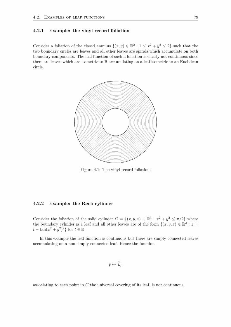
4.2. Examples of leaf functions 79

4.2.1 Example: the vinyl record foliation

Consider a foliation of the closed annulus (x, y) ∈ R2 : 1 ≤ x2 + y2 ≤ 2 such that thetwo boundary circles are leaves and all other leaves are spirals which accumulate on bothboundary components. The leaf function of such a foliation is clearly not continuous sincethere are leaves which are isometric to R accumulating on a leaf isometric to an Euclideancircle.

Figure 4.1: The vinyl record foliation.

4.2.2 Example: the Reeb cylinder

Consider the foliation of the solid cylinder C = (x, y, z) ∈ R3 : x2 + y2 ≤ π/2 wherethe boundary cylinder is a leaf and all other leaves are of the form (x, y, z) ∈ Rd : z =t− tan(x2 + y2)2 for t ∈ R.

In this example the leaf function is continuous but there are simply connected leavesaccumulating on a non-simply connected leaf. Hence the function

p 7→ Lp

associating to each point in C the universal covering of its leaf, is not continuous.


Figure 4.2: A section of the Reeb cylinder.

4.2.3 Example: the Reeb component

One may take the quotient space of a Reeb cylinder by a translation along the axis toobtain a foliation of the solid torus normally called a Reeb component.

The leaf function of a Reeb component is not continuous since for any sequence xn ofinterior points converging to a boundary point x one has that the sequence of leaves Lxnconverges to a cylinder M while the leaf Lx is a torus.

We notice that the cylinderM is a covering space of the torus leaf Lx. Furthermore onecan choose a covering map fromM to Lx in such a way that the image of the fundamentalgroup of M is exactly the set of curves in Lx without holonomy.

Hence one sees that in this example the function

x 7→ Lxhol

associating to each point the holonomy covering of its leaf (see Section 4.9), is continuous.

Figure 4.3: Half a Reeb component.

4.2. Examples of leaf functions 81

4.2.4 Example: the broken record foliation

Consider a foliation of the closed annulus which is obtained by pasting a copy of the vinylrecord foliation with a trivially foliated annulus (i.e. foliated by parallel circles).

The holonomy of leaves in the trivially foliated annulus is trivial and hence they co-incide with their holonomy covers. However a sequence of such leaves can be chosen toconverge to the single circular leaf separating the two components. This leaf has non-trivial holonomy and hence its holonomy cover is isometric to R. Hence in this exampleon sees that the function

x 7→ Lxhol

is not continuous.

Figure 4.4: A broken record foliation. Circu-lar leaves with trivial holonomy accumulateon a circular leaf with non-trivial holonomy.

4.2.5 Example: the Reeb transition

The following example was introduced by Reeb in [Ree48].Consider the product Riemannian manifold S2 × S1 × S1 where S2 = (x, y, z) ∈ R2 :

x2 + y2 + z2 = 1 is the standard two-dimensional sphere, and S1 = z ∈ C : |z| = 1 thestandard circle. We consider the coordinates ((x, y, z), eis, eit) and the one forms

ω1 = dtω2 =

((1− sin(t))2 + x2) ds+ sin(t)dx

The conditions of Frobenius’ integrability theorem (see [CLN85, Theorem 2, pg. 185])are satisfied and hence there is a unique two-dimensional foliation such that the tangentspace of each leaf is contained in the kernel of ω1 and ω2. The equation ω1 = 0 forvectors tangent to the foliation implies that each leaf is contained in a set of the formS2 × S1 × constant and hence we may consider the foliation as a family of foliations onS2 × S1 parametrized by t.


When sin(t) = 0 it is easy to verify that one obtains the foliation of S2 × S1 by leavesof the form S2 × constant. However, when sin(t) = 1 one has

ω2 = x2ds+ dx

so that the torus in S2 × S1 defined by x = 0 is a leaf, while the other leaves are planesparametrized by functions of the form

(x, y, z) 7→ ((x, y, z), ei(c+1/x))

on the hemispheres x < 0 and x > 0, for different values of the constant c.Whenever sin(t) 6= 0 one obtains a foliation of S2 × S1 by spheres such that all leaves

are obtained by applying a rotation to the S1 components of a single leaf (i.e. they areall graphs of functions from S2 to S1 which in fact can be written explicitly).

Hence the set of spherical leaves is given by sin(t) 6= 1, and the set of non-compactleaves is defined by sin(t) = 1, x 6= 0.

One can explain this example geometrically. By pasting two copies of the partition ofthe solid torus D×S1 into closed disks D×constant one can obtain the trivial foliationof S2 × S1 by leaves of the form S2 × constant. Pushing each disk at its center in thedirection of the central circle of the solid torus one deforms the foliation but all leaves arestill copies of S2. This is done in such a way that the number of turns each disk doesaround the solid torus diverges, at which point the boundary torus becomes a leaf andwe obtain a foliation of S2 × S1 by two Reeb components. We call this process a Reebtransition.

Reeb noticed that in any such example there must be spherical leaves with arbitrarilylarge volume. We will show that this is a consequence of the regularity properties of theleaf function.

Figure 4.5: A Reeb transition: the trivial partition of a solid torus into disks is deformedinto a Reeb component.

4.3 Regularity of leaf functionsIn this section we state and prove our two main results after which we discuss applicationsto Reeb-type stability results and the Reeb transition example of the previous section.

4.3.1 Regularity theorems

A sequence of pointed complete connected Riemannian manifolds of the same dimension(Mn, on, gn) is said to smoothly converge to a pointed complete Riemannian manifold(M, o, g) if there exists for each r > 0 a sequence of pointed smooth embeddings fn :Br(o)→Mn of the open ball of radius r centered at o into Mn defined for n large enoughwith the property that the pullback Riemannian metrics f∗ngn converge smoothly to g onall compact subsets of Br(o) (see [Pet06, Chapter 10.3.2] and Section 4.7).

4.3. Regularity of leaf functions 83

In principle smooth convergence of a sequence of manifolds is much stronger thanGS-convergence of the same sequence. However we can use compactness results fromRiemannian geometry to obtain the following results.

Theorem 4.1 (Precompactness of the leaf function). Let X be a compact d-dimensionalfoliation. Then the leaf function of X takes values in a compact subset M of GS whichcontains only complete Riemannian manifolds of dimension d. Furthermore smooth andGS-convergence are equivalent onM.

Proof. We establish in Section 4.8 that there exists r > 0 and a sequence Ck such thatthe injectivity radius of all leaves is at least r and the tensor norm of k-th derivative ofthe curvature tensor of any leaf is at most Ck.

Hence all leaves belong to the set M of (isometry classes of) pointed complete d-dimensional Riemannian manifolds with geometry bounded by (r, Ck) (see Section 4.4).

We establish in Theorem 4.11 that M is GS-compact and that a sequence in Mconverges smoothly if and only if it GS-converges.

Corollary 4.2. If xn is a sequence converging to a point x in a compact foliation X andthe sequence of leaves Lxn GS-converges to a pointed metric space M then, in fact, M isa smooth complete Riemannian manifold and Lxn converges smoothly to M . In particularif M is compact then Lxn is diffeomorphic to M for all n large enough.

By a Riemannian covering we mean a pointed local isometry f : M → N betweencomplete pointed Riemannian manifolds. If such a covering exists we say that M is aRiemannian covering (or just a covering) of N and that N is covered by M . See Section4.9 for the definition of the holonomy covering of a leaf.

Theorem 4.3 (Semicontinuity of the leaf function). Let X be a compact foliation and xnbe a sequence converging to a point x ∈ X. If the sequence of leaves Lxn GS-converges toa pointed Riemannian manifold M then M is a Riemannian covering space of Lx and iscovered by Lx

hol.

Proof. By Theorem 4.1 the leaf function takes values in a compact subspace of GS whereGromov-Hausdorff and smooth convergence are equivalent. Hence M is a complete Rie-mannian manifold and the sequence converges smoothly to M .

By smooth convergence (see Section 4.7), for each r > 0 there is a sequence of pointedembedding fn,r : Br(oM )→ Lxn (defined for n large enough) such that |f∗n,rgLxn − gM |gMconverges uniformly to 0 on Br(oM ). We show in Lemma 4.34 that this implies thatthe maps fn,r have a subsequence which converges locally uniformly to a local isometryfr : Br(oM )→ Lx.

Now consider the family of functions fr : Br(oM )→ Lx when r → +∞. Since all thesefunctions are local isometries one obtains a local isometry f : M → Lx as a the uniformlimit on compact subsets frk for some subsequence rk → +∞. Hence M is a Riemanniancovering of Lx via the covering map f .

Suppose that for some pair of distinct points x, y ∈ M one has f(x) = f(y) and letα : [0, 1] → M be a curve joining x and y. Take r > 0 large enough so that Br(oM )contains α([0, 1]) and let fn,r : Br(oM ) → Lxn be a sequence of embeddings as abovewhich converges locally uniformly to f on Br(oM ).

Since each fn,r is injective and the pullback metrics converge to gM the leafwise distancebetween fn,r(x) and fn,r(y) is bounded below by a positive constant for n large enough.


However since fn,r α converges uniformly to f α we obtain that the holonomy alongthe closed curve f α is non-trivial (see Corollary 4.31).

We have established that any closed curve in Lx having a lift under f which is notclosed has non-trivial holonomy. In particular the lift of any curve with trivial holonomyin Lx is closed inM and hence the image of the fundamental group ofM under f containsthe subgroup of curves with trivial holonomy. By the classification of covering spaces (seeLemma 4.27) Lx

hol is a Riemannian cover of M .

4.3.2 Applications to continuity and Reeb stability

The main result of [EMT77] is that in any foliation the set of leaves without holonomy isresidual. Combined with Theorem 4.3 we obtain that the leaf function is continuous on aresidual set. Potential applications of this result to the study of quasi-isometry invariantsof leaves are discussed by Álvarez and Candel in [ÁC03, Section 2].

Corollary 4.4 (Álvarez-Candel continuity theorem). The leaf function of any compactfoliation is continuous on the set of leaves without holonomy. In particular the set ofcontinuity points contains a residual set.

Smooth convergence of a sequence to a compact manifold implies that the sequenceelements are eventually diffeomorphic to the limit. Combined with Theorem 4.3 oneobtains Reeb’s local stability theorem (see [Ree47, Theorem 2]).

Corollary 4.5 (Reeb’s local stability theorem). Let X be a compact foliation and x ∈ Xbe such that Lx is compact. Then there exists a neighborhood U of x such that Ly isdiffeomorphic to Lx for all y ∈ U .

The same argument gives the usual generalization of Reeb’s stability theorem to com-pact leaves with trivial or finite holonomy (see for example [CLN85, pg. 70]).

Corollary 4.6 (Stability of compact leaves with finite holonomy). Let X be a compactfoliation and x ∈ X be such that Lx

hol is compact. Then there is a neighborhood U of xsuch that for each y ∈ U the leaf Ly is compact and diffeomorphic to a covering space ofLx.

We say X is a foliation by compact leaves if all leaves are compact. The volumefunction of such a foliation is the function

x 7→ vol (Lx)

associating to each leaf its volume (which is finite). Since a Riemannian covering haslarger volume then the space it covers one obtains the following.

Corollary 4.7 (Volume function semicontinuity). Let X be a compact foliation by compactleaves. Then the volume function of X is lower semicontinuous.

Notice that since any sequence of leaves has a smoothly convergent subsequence weobtain the following part of Epstein’s structure theorem (see [Eps76, Theorem 4.3]).

Corollary 4.8 (Epstein). Let X be a compact foliation by compact leaves whose volumefunction is bounded. Then every point x ∈ X has a neighborhood U such that for all y ∈ Uthe leaf Ly is diffeomorphic to a finite covering of Lx.

4.3. Regularity of leaf functions 85

We say a foliation X has codimension k if it admits an atlas by foliated charts hi :Ui → Rd × Ti, i ∈ I with Ti = Rk for all i. Under this hypothesis X is automatically atopological manifold.

Notice that any holonomy transformations of a codimension one foliation will be ahomeomorphism between two open subsets of R. We say a codimension one foliation istransversally orientable if every holonomy transformation associated to a closed chain ofcompatible charts is increasing.

The following elementary lemma implies that in a transversally oriented codimensionone foliation by compact leaves all leaves have trivial holonomy (here we denote by fn(x) =f(f(· · · f(x) · · · )) the n-th iterate of the point x under the function f and notice that inorder for it to be well defined fk(x) must belong to the domain of f for all k = 0, . . . , n−1):

Lemma 4.9. Let h : U → V ⊂ R be an increasing homeomorphisms between two neigh-borhoods of 0 ∈ R such that h(0) = 0. Then either h is the identity map or there existsx ∈ U and f = h±1 such that the set fn(x) : n ≥ 0 is well defined and infinite.

Epstein established in [Eps72] that a flow on a 3-manifold for which all orbits areperiodic has the property that the periods are bounded. This was later generalized tostate that compact codimension two foliations by compact leaves have bounded volumefunctions (see [EMS77]). Notice that these results are very subtle since they are falsefor foliations of codimension 3 or more (see [EV78]). The codimension one case followsdirectly from our results and the above elementary lemma.

Corollary 4.10. Let X be a connected compact transversally oriented codimension onefoliation. Then the leaf function of X is continuous. In particular all leaves are diffeo-morphic and the volume function is continuous.

For tranversally oriented codimension one foliations of connected manifolds Reeb’slocal stability combines with properties of one dimensional dynamics in the spirit of thelemma above to yield Reeb’s global stability theorem (see [Ree47, Theorem 3] and [CLN85,pg. 72]) which states that if a leaf has a compact universal cover than all leaves arediffeomorphic.

In view of these results one might conjecture that the set of leaves with compactuniversal cover, besides being open, is always closed. However this is false as shown bythe Reeb transition example given in Section 4.2.5. We will now discuss some aspects ofthis example.

The fact that in the Reeb transition there must be spheres with arbitrarily large volumefollows from Corollary 4.4 and the smooth convergence given by Theorem 4.1. To see thisconsider a sequence of points xn belonging to compact leaves which converge to a pointx whose leaf is non-compact and notice that the sequence of manifolds Lxn smoothlyconverge to Lx.

Consider now in the same example a sequence xn on spherical leaves which converges toa point x on the single torus leaf. By Theorem 4.3 any smooth limit point of the sequenceLxn must either be a finite covering of the torus Lx or the cylinder Lx

hol. The first caseis impossible because convergence to a compact limit would imply that the manifolds inthe sequence Lxn are eventually diffeomorphic to the limit manifold which would have tobe a torus. Hence the sequence of spheres Lxn converges smoothly to the cylinder Lx

hol.


4.4 Uniformly bounded geometry

In this section we prove that certain subsets of GS consisting of manifolds with ‘uniformlybounded geometry’ are compact and that furthermore smooth and GS-convergence coin-cide on them. This result was used in the proof of Theorem 4.1.

4.4.1 Spaces of manifolds with uniformly bounded geometry

We say a complete d-dimensional Riemannian manifold has geometry bounded by r > 0and a sequence Ck if the injectivity radius ofM is at least r at all points and the curvaturetensor of M satisfies

|∇kR| ≤ Ck

for all k, where ∇ denotes the covariant derivative and we are using the tensor normsinduced by the Riemannian metric.

We useM (d, r, Ck) to denote the subset of GS consisting of all isometry classes ofd-dimensional complete pointed Riemannian manifolds with geometry bounded by r andthe sequence Ck.

An element ofM (d, r, Ck) is represented by a triplet (M, oM , gM ) and two tripletsrepresent the same element if there is a pointed isometry between them. We will sometimeswrite M ∈ M (d, r, Ck) in which case it is implied that the basepoint will be denotedby oM and the Riemannian metric by gM .

4.4.2 A smooth compactness theorem

Usually GS-convergence of a sequence of manifolds is much weaker than smooth con-vergence. However we will show they are equivalent on sets of manifolds with uniformbounded geometry.

To understand this it might be helpful to consider the following fact: Let F be a C1

compact family of functions from the interval [0, 1] to R. Then if a sequence fn in Fconverges uniformly to a limit f , in fact f ∈ F and the derivatives f ′n converge uniformlyto f ′.

The proof can also be thought of as an application of the fact that a continuous bijectivefunction whose domain is compact has a continuous inverse (in the setting of the previousparagraph the domain would be F with the C1-topology the codomain would be the sameset with the C0-topology and function would be the identity). The difficulty in our case isin establishing compactness of the domain plus a subtle technical point which is discussedimmediately after the proof.

We will now state the main result of this section.

Theorem 4.11. Let M = M (d, r, Ck) for some choice of dimension d, radius r, andsequence Ck. Then M is a compact subset of GS on which GS-convergence and smoothconvergence are equivalent.

Proof with gap. The proof rests on the following facts

1. The setM is precompact with respect to smooth convergence.

2. The setM is closed under smooth convergence.

3. Smooth convergence implies pointed Gromov-Hausdorff convergence.

4.4. Uniformly bounded geometry 87

We will establish facts 1 and 2 in sections 4.5 and 4.6 respectively.

Fact 3 is generally accepted (e.g. see [Pet06, Section 10.3.2] and [BBI01, Section 7.4.1])but we include a proof in the next subsection for completeness.

Using these facts the proof proceeds as follows.

Given a sequenceMn inM we may, using smooth precompactness, extract a smoothlyconvergent subsequence Mnk with limit M . SinceM is closed under smooth convergencewe have M ∈ M. Finally, since smooth convergence implies pointed Gromov-Hausdorffconvergence one has

limn→+∞

dGS(Mnk ,M) = 0.

This establishes thatM is a compact subset of GS.

Suppose now that some sequenceMn inM converges in the pointed Gromov-Hausdorffsense to M ∈ M. Since any subsequence of Mn will have a further subsequence whichconverges smoothly and any smooth limit must in fact coincide with M we obtain thatthe original sequence Mn converges smoothly to M .

There is a gap in the above proof which is illustrated by the following example (seeFigure 4.6).

Consider the sequence of functions indexed on finite strings of zeros and ones definedby

fa1...ar : [0, 1]→ R

fa1...ar(x) =

1 ifr∑

k=1ak2−k < x < 2−r +

r∑k=1

ak2−k.

0 otherwise.

The sequence does not converge Lebesgue almost surely to any function. However anysubsequence has a further subsequence which converges almost surely to 0. In particularthe arguments in our proof above would imply that L2 convergence and almost sureconvergence coincide on the set of functions 0 ∪ fa1...ar but this conclusion is false.

To exclude this type of behavior it suffices to show that smooth convergence comesfrom a topology. We do this in Section 4.7.


f0

x0 112

0

1

f1

x0 112

0

1f00

x0 112

14

34

0

1

f01

x0 112

14

34

0

1

f10

x0 112

14

34

0

1

f11

x0 112

14

34

0

1

Figure 4.6: Six elements of a sequence of functions which does not converge almost surelyto 0 but has no other limit points.

4.4.3 Smooth vs Gromov-Hausdorff convergence

For the readers convenience we present a proof of the fact that smooth convergence isstronger than GS-convergence. The key ideas are contained in the proof of part 2 of[BBI01, Theorem 7.3.25] and the indications given in Section 7.4.1 of the same reference.

Lemma 4.12. If a sequence (Mn, on, gMn) converges smoothly to (M, o, g) then it alsoGS-converges to the same limit.

Proof. We must show that for each r > 0 the sequence of pointed compact metric spacesBr(on) (where the metric is inherited from Mn) converges in the Gromov-Hausdorff senseto Br(o).

By smooth convergence (see Section 4.7) given r > 0 there exists a sequence of smoothpointed embeddings fn : B3r(o) → Mn with the property that the pullback metrics gn =f∗ngMn satisfy

an = sup|gn(x)− g(x)|g : x ∈ B3r(o) → 0

when n→ +∞.Notice that whenever an = 0 one has that Br(o) is isometric to Br(on) via fn so that

there is nothing to prove. Hence we may assume without loss of generality in what followsthat an 6= 0. Also, since we are only interested in behavior when n→ +∞ we may assumethat an < 1.

Let d be the Riemannian distance of M and dn be the pullback under fn of theRiemannian distance on Mn. Since the shortest curve between fn(x) and fn(y) might inprinciple exit fn(B3r(o)) it is not necessarily true that dn equals the distance on B3r(o)induced by the metric gn.

4.5. Smooth precompactness 89

However notice that if v is a tangent vector in B3r(o) of unit norm for g then

|gn(v, v)− 1| ≤ an

so that the gn norm of v is between (1 − an)1/2 and (1 + an)1/2. This implies that thegn-length of any curve in B3r(o) is within a multiplicative factor b±1

n of its g-length wherebn = max

((1− an)−1/2, (1 + an)1/2

). In particular, for n large enough, the Riemannian

distance induced by gn on B3r(o) coincides with dn when restricted to Br(o).The previous comparison of lengths of curves also implies for n large that

|dn(x, y)− d(x, y)| ≤ (bn − 1)d(x, y) ≤ 2r(bn − 1)

for all x, y ∈ Br(o) (the first inequality relies on the fact that 1 − b−1n ≤ bn − 1 which is

true since bn ≥ 1).Following the proof of part 2 of [BBI01, Theorem 7.3.25] we consider for each n the

distance dn on the disjoint union Br(o) t Br(o) which coincides with d on the left-handcopy, with dn on the right-hand copy and for x, z in different copies is defined by

dn(x, z) = infd(x, y) + 2r(bn − 1) + dn(y, z) : y ∈ Br(o)

.

The Hausdorff distance between the two copies of Br(o) with the above defined distanceis less than 3r(bn−1) and therefore goes to 0 when n→ +∞. This shows that the Gromov-Hausdorff distance between Br(o) and fn(Br(o)) (the later inheriting its metric from Mn)converges to 0 when n→ +∞.

To conclude it suffices to establish that the Hausdorff distance (with respect to theRiemannian distance on Mn) between fn(Br(o)) and Br(on) goes to 0 when n → +∞.This follows from our comparison of d and dn since fn(Br(o)) contains the ball of radiusb−1n r and is contained in the ball of radius bnr centered at on.

4.5 Smooth precompactnessIn this section we prove that sets of manifolds with uniformly bounded geometry areprecompact with respect to smooth convergence. This was used in the proof of Theorem4.11.

We recall (see [Pet06, Chapter 10] and Section 4.7) that, in similar fashion to the def-inition of smooth convergence, a sequence of complete Riemannian manifolds (Mn, on, gn)is said to converge Ck to (M,o, g) if for each r > 0 there exists a sequence of smoothpointed embeddings fn : Br(o)→Mn (defined for large enough n) such that the pullbackmetrics f∗ngn converge Ck to g on compact subsets of Br(o).

Lemma 4.13. All subsets of GS of the form M = M (d, r, Ck) are sequentially pre-compact with respect to smooth convergence.

Proof. For each M ∈ M we consider the atlas A by normal coordinates on the balls ofradius r′ given by Lemma 4.16 below.

A theorem of Eichhorn (see Lemma 4.15 below) shows that there exists a sequence Cknorsuch that all the metrics on Br′ obtained from such coordinates have coefficients whichsatisfy

|∂i1 · · · ∂ikgij | ≤ Cknor

for all choices of indices i1, . . . , ik.


Furthermore we establish in Lemma 4.16 that there is a sequence Cktran bounding thek-th order partial derivatives of the transition maps of any such atlas A and that theEuclidean and Riemannian norms on Br′ differ at most by a multiplicative factor of 2±1/2.

This shows that for each k there exists Q such that all manifold inM have Ck normless than or equal to Q on a scale of r in the sense of Petersen (see the definition insubsection 4.5.1 below).

Applying Petersen’s compactness theorem (see Theorem 4.14 below) one obtains thatM is Ck precompact for all k, and hence smoothly precompact as claimed.

4.5.1 Norms and sequential compactness

Following [Pet06, Chapter 10.3.1] (taking, for simplicity, α = 1 in his notation) we saythat a manifold M has Ck-norm less than or equal to Q on a scale of r if there exists anatlas A of M which satisfies the following properties:

1. Every ball of radius e−Qr/10 is contained in the domain of some chart in A.

2. For each chart ϕ ∈ A one has |Dϕ| ≤ eQ and |Dϕ−1| ≤ eQ, where Dϕ is the tangentmap to the chart and one uses the operator norm between the tangent space of Mwith the Riemannian metric and Euclidean space with the usual Euclidean metric.

3. For each chart ϕ ∈ A and each 0 ≤ i ≤ k the partial derivatives of order i of thecoefficients of ϕ∗gM are Q/(ri+1)-Lipschitz.

4. For each ϕ1, ϕ2 ∈ A the Ck+2-norm (i.e. sum of suprema of absolute values of allpartial derivatives up to order k + 2) of the transition map ϕ2 ϕ−1

1 is less than orequal to (10 + r)eQ.

We now restate Petersen’s [Pet06, Theorem 72] as we will use it.

Theorem 4.14 (Petersen). For any positive constants r and Q the class of pointed, com-plete, d-dimensional Riemannian manifolds with Ck-norm less than or equal to Q on ascale of r is sequentially compact with respect to Ck convergence.

4.5.2 Normal coordinates

We recall that a normal parametrization of a manifold M ∈M (d, r, Ck) at a point p isa function ψ : Rd →M satisfying

ψ(x) = expψ(0) f(x)

where exp : Tψ(0)M → M is the Riemannian exponential map and f : Rd → Tψ(0)M is alinear isometry between Rd and the tangent space Tψ(0)M at ψ(0).

If M ∈ M (d, r, Ck) then any normal parametrization ψ is a diffeomorphism whenrestricted to the ball Br of radius r centered at 0 ∈ Rd. Hence the pullback g = ψ∗gM ofthe Riemannian metric of M to Br is also a Riemannian metric (i.e. non-degenerate).

We recall that the coefficients of a metric g defined on some open subset of Rd are thefunctions

x 7→ g(x)(ei, ej) = gij(x)

where e1, . . . , ed is the canonical basis of Rd.The coefficients obtained in this manner from manifolds inM (d, r, Ck) are uniformly

Ck bounded as is shown by the following lemma (see [Eic91, Corollary 2.6]).


Lemma 4.15 (Eichhorn). Given M = M (d, r, Ck) for each k ≥ 0 there exists aconstant Cknor such that if g = ψ∗gM is a metric on Br obtained by pulling back the metricof some manifold M ∈M via a normal parametrization ψ then one has:

|∂i1 · · · ∂ikgij | ≤ Cknor

for all indices i, j, i1, . . . , ik.

4.5.3 Transition maps

This subsection is devoted to establishing the following uniform estimate for the derivativesof transition maps between normal coordinates.

Lemma 4.16. Given M = M (d, r, Ck) there exists r′ < r and for each k ≥ 0 aconstant Cktran such that the k-th order partial derivatives of any transition map betweennormal coordinates on balls of radius r′ in any manifold M ∈M are bounded in absolutevalue by Cktran.

For partial derivatives of order one and two the above result can be compared toLemma 3.4 and Lemma 4.3 of [Che70].

The first derivative of the change of coordinates between maximal normal coordinatesbased at the north and south pole on the standard two dimensional sphere is not bounded.This shows that it’s indeed necessary to take r′ < r in the above lemma.

Our proof proceeds in three steps. First we bound the k-th order covariant derivativeof any curve of the form t 7→ x + tv for any metric on the Euclidean ball of radius r′in Rd obtained by pullback from a normal parametrization of a manifold inM. Second,we bound the the actual (Euclidean) k-th order derivative of any curve whose covariantderivatives satisfy the previously obtained bounds (the point here being that covariantderivatives are invariant under the transition maps). Finally, combining the precedingresult one obtains a bound for the k-th derivative of any transition map along any straightline which implies the same bound is satisfied for the partial derivatives of order k (thisamounts to the statement that a symmetric k-linear function attains its maximum normon the diagonal, see [Wat90] for a proof).

To begin we recall that the Christoffel symbols of a metric on an open subset of Rdwith coefficients gij are given by

Γkij = 12g

kl (∂jgil + ∂iglj − ∂lgij)

where gij are the coefficients of the inverse of the matrix (gij) and summation is impliedover the repeated indices of each term.

In what follows we use Bs for the open Euclidean ball of radius s centered at 0 ∈ Rd.

Lemma 4.17. GivenM =M (d, r, Ck) there exists r′ < r and for each k ≥ 0 a constantC ′k such that for any metric g on Br′ obtained by pullback from a normal parametrizationof a manifold M ∈M one has:

1. The k-th order partial derivatives of the metric coefficients gij, the coefficients of theinverse matrix gij, and the Christoffel symbols Γlij, are bounded in absolute value byC ′k for all k.

2. For all v ∈ Rd and x ∈ Br′ one has 2−1|v| ≤ |v|g(x) ≤ 2|v| where |v| is the Euclideannorm of v and |v|g(x) its norm with respect to the inner product g(x).


Proof. Notice that for any of the coefficients gij under consideration one has (gij(0)) = (δij)where the right-hand side is the d× d identity matrix. Let K be a compact neighborhoodof the identity matrix such that any inner product whose matrix of coefficients (i.e. thematrix whose entry in the i-th row and j-th column is the inner product between the i-thand j-th vectors of the canonical basis of Rd) is in K satisfies property 2 above.

Since one has a uniform bound C1nor (given by Lemma 4.15) for the first order deriva-

tives of gij on Br there exits r′ < r (depending only on this C1nor) such that for all the

metrics under consideration (gij(x)) belongs to K for all x ∈ Br′ .By Lemma 4.15 one has uniform bounds on the partial derivatives of the metric co-

efficients gij on Br (and in particular on Br′). Combining this with the fact that matrixinversion is smooth on K one obtains uniform bounds for the partial derivatives of allorders of the inverse matrix (gij) on Br′ . From this one can bound the partial derivativesof the Christoffel symbols as well.

The covariant derivative of a vector field v(t) over a curve x(t) in Rd with respect toa metric with Christoffel symbols Γkij is given by

∇x′v = v′ + Γkij(xi)′vjek (4.1)

where a superscript i denotes the i-th coordinate and ′ denotes derivative with respect tot. We convene that ∇0

x′v(t) = v(t) and define inductively ∇k+1x′ v(t) = ∇x′∇kx′v(t).

Lemma 4.18. FixM =M (d, r, Ck) and let C ′k and r′ be given by Lemma 4.17. Thereexists a sequence C ′′k such that for any metric g on Br′ obtained by pullback from a normalparametrization of a manifold M ∈M and any curve of the form

x(t) = x0 + tv

where x0 ∈ Br′ and |v| = 1 one has

|∇kx′x′|g ≤ C ′′k

for all k ≥ 0.

Proof. From Lemma 4.17 the Riemannian norm of v is bounded by 2 at all points in Br′ .This shows that one can take C ′′0 = 2.

In order to bound the higher order covariant derivatives define inductively

v2(t) = ∇x′v = vivjΓkijek

andvn+1(t) = ∇x′vn(t) = v′n + vivjnΓkijek.

Since the coordinates vi of v are constants of absolute value less than or equal to 1 theEuclidean norm of vn+1 can be bounded in terms of that of vn and the derivatives of theChristofell symbols. This is possible and is equivalent to bounding the Riemannian normdue to Lemma 4.17.

We denote by x(k)(t) denote the k-th (Euclidean) derivative of a curve in Rd.


Lemma 4.19. FixM =M (d, r, Ck) and let C ′′k and r′ be given by Lemma 4.17. Thereexists a sequence C ′′′k such that for any metric g on Br′ obtained by pullback from a normalparametrization of a manifold M ∈M and any curve x(t) satisfying

|∇kx′x′|g ≤ C ′′k

for all k ≥ 0 one has|x(k)(t)| ≤ C ′′′k

for all k ≥ 0.

Proof. By Lemma 4.17 the Euclidean and Riemannian norms differ at most by a factor of2±1/2.

In particular one can take C ′′′0 = 2C ′′0 and the Euclidean norm of

∇x′x′ = x′′ + Γkij(xi)′(xj)′ek

is bounded by 2C ′′1 .Since one has |x′| ≤ 2C ′′0 one obtains from the last equation a bound for |x′′|.The higher order case follows by induction since there is a single term in ∇kx′x′ which

is equal to x(k+1) and the rest can be bounded in terms of lower order derivatives of x andthe derivatives of the Christoffel symbols.

We now complete the final step for the proof of Lemma 4.16.

Lemma 4.20. Let f : U ⊂ Rd → Rd be a smooth function satisfying

|g(k)(0)| ≤ C ′′k

for all k ≥ 0 and g of the form g(t) = f(x + tv) with |v| = 1 and x ∈ U . Then for allx ∈ U one has

|∂i1 · · · ∂ikf(x)| ≤ C ′′k

for all k ≥ 0 and i1, . . . , ik ∈ 1, . . . , d.

Proof. Define inductively

Dxf(v) = limh→0

f(x+ hv)− f(x)h

D2xf(v1, v2) = lim

h→0

Dx+hv1f(v2)−Dxf(v2)h

Dk+1x f(v1, . . . , vk+1) = lim

h→0

Dkx+hv1

f(v2, . . . , vk+1)−Dkxf(v2, . . . , vk+1)

h.

Letting P kx f(v) = Dkxf(v, . . . , v) we have by hypothesis and multilinearity that |P kx f(v)| ≤

C′′k |v|k.Since partial derivatives commute the multilinear function Dk

xf : (Rd)k → Rd is sym-metric and P kx f determines Dk

xf by polarization. This implies a bound for the mixedpartial derivatives, and in fact one has |Dk

xf(v1, . . . , vk)| ≤ C′′k |v1| · · · |vk| as shown in

[Wat90].


4.6 Curvature and injectivity radiusIn this section we prove that sets of manifolds with uniform bounded geometry are closedwith respect to smooth convergence. This was used in the proof of Theorem 4.11.

Lemma 4.21. SupposeM =M (d, r, Ck) for some value of the parameters. If (Mn, on, gn)is a sequence inM converging smoothly to (M,o, g) then M ∈M.

Proof. The fact that the injectivity radius ofM is larger than or equal to r follows becausethe injectivity radius is upper semicontinuous with respect to smooth convergence as wewill show in the next subsection (see Lemma 4.22).

We will now establish that M satisfies the curvature bounds

|∇kR|g ≤ Ck.

Let (gij) be the matrix of coefficients of a metric g on an open subset of Rd and (gij)the inverse matrix. The g norm of a (p, q) tensor field 1

T = aiq+1,...,ip+qi1,...,iq

ei1 ⊗ · · · ⊗ eiq ⊗ eiq+1 ⊗ · · · eip+q

(where we denote by ei the canonical basis and ei the dual basis of Rd) is given by

|T |2g = aiq+1,...,ip+qi1,...,iq

ajq+1,...,jp+qj1,...,jq

gi1j1 · · · giqjqgiq+1jq+1 · · · gip+qjp+q .

The curvature tensor of g is the (1, 3)-tensor field R = Rlijkei ⊗ ej ⊗ ek ⊗ el given by

(e.g. see [Bre10, Section 5])

Rlijk = ∂jΓlki − ∂kΓljk + ΓkjmΓmki − ΓlkmΓmji

where the Christoffel symbols Γkij are defined by

Γkij = 12g

kl(∂igil + ∂jgjl − ∂lgij).

Since matrix inversion is smooth the two formulas above prove that if a sequence ofmetrics gn converges uniformly on compact sets to g then the norm of their curvaturetensors converge pointwise to that of g.

Similarly, for each k the covariant derivative ∇kR is a (1, 3 + k)-tensor field whosecoefficients are smooth functions of the partial derivatives of the coefficients gij and gij .This shows that the bound |∇kR| ≤ Ck passes to the limit when a sequence of manifoldsconverges C∞ to another. Hence one has that the limit manifold M of the the sequenceMn also satisfies these bounds.

4.6.1 Semicontinuity of the injectivity radius

Continuity of the injectivity radius with respect to a varying family of metrics on a singlecompact manifold was established in [Ehr74] and [Sak83].

The injectivity radius is not continuous under smooth convergence of pointed manifoldsas can be seen by considering a metric g on R2 which has finite injectivity radius but isflat outside of a compact set. In this setting the sequence of pointed manifolds (R2, xn, g)

1. In all tensor calculations we use the convention that summation is implied over indices which arerepeated in a term

4.6. Curvature and injectivity radius 95

will smoothly converge to R2 endowed with the Euclidean metric if xn → ∞ when n →+∞. Hence we have a sequence of manifolds with finite and constant injectivity radiusconverging to a manifold whose injectivity radius is infinite.

Figure 4.7: An asymptotically flat surface with finite injectivityradius. Changing the basepoint gives an sequence converging to alimit whose injectivity radius is infinite.

However, upper semicontinuity still holds as we will now show.

Lemma 4.22 (Semicontinuity of the injectivity radius). The injectivity radius is uppersemicontinuous with respect to smooth convergence.

Proof. Suppose for the sake of contradiction that there is a sequence (Mn, on, gn) withthe injectivity radius of each term larger than or equal to some r > 0 which convergessmoothly to a manifold (M,o, g) whose injectivity radius is strictly less than r.

By Proposition 19 and Lemma 14 of [Pet06, pg. 139-142], there exists a geodesicα : [0, 1]→M of length L < r and some other smooth curve β : [0, 1]→M with the sameendpoints with length L′ < L.

By the definition of smooth convergence there is an open set Ω containing α([0, 1]) andβ([0, 1]) and a sequence of pointed embeddings fn : Ω → Mn such that f∗ngn convergesC∞ to g on compact subsets of Ω.

Consider αn : [0, 1]→M the geodesic for the metric f∗ngn with initial condition α′(0).We claim that αn(1)→ α(1) and that the f∗ngn length of αn converges to L when n→ +∞.By covering α([0, 1]) with a finite number of charts and noticing that in each chart thecoefficients of f∗ngn converge C∞ on compact sets to those of g, this follows from continuityof solutions to ordinary differential equations with respect to the vector field (see [DK00,Theorem B3, pg. 333]). We omit further details.

Smooth convergence of f∗ngn to g implies that the f∗ngn length of β converges to L′ andthe f∗ngn distance between β(1) and αn(1) converges to 0.

Hence for n large enough the manifold Mn contains a geodesic of length strictly lessthan r which is not the shortest curve between its endpoints. By the Hopf-Rinow theoremwe will find two geodesics of length strictly less than r joining the same endpoints in Mn

contradicting the fact that the injectivity radius of Mn is larger than or equal to r.


4.7 Smooth convergence and tensor normsIn this section we discuss in detail the definition of Ck and smooth convergence of pointedRiemannian manifolds. In particular we provide a coordinate free definition of convergencein terms of tensor norms and prove that it is equivalent to definition given in [Pet06,Chapter 10.3.2].

We also establish that Ck and smooth convergence on certain subsets of GS comesfrom a topology, a fact that was used in the proof of Theorem 4.11.

4.7.1 Coordinate free definition of convergence

Following [Pet06, 10.3.2] a sequence (Mn, on, gn) of pointed connected complete Rieman-nian manifolds is said to converge Ck to (M,o, g) if for every r > 0 there exists a domain Ωcontaining Br(o) and (for n large enough) a sequence of pointed embeddings fn : Ω→Mn

such that fn(Ω) ⊃ Br(on) and f∗ngn converges Ck to g on compact subsets of Ω. Smoothconvergence is by definition Ck convergence for all k.

Recall that the coefficients of a Riemannian metric g defined on an open subset U ofRd are the functions

x 7→ g(x)(ei, ej) = gij(x)

where e1, . . . , ed is the canonical basis of Rd.By Ck convergence of f∗ngn to g on compact subsets of Ω we mean that for any smooth

parametrization h : U → V ⊂ Ω the coefficients of the metrics h∗f∗ngn converge to thoseof h∗g in the Ck topology on every compact subset of U .

To see that the restriction to compact subsets of U is necessary consider the sequenceof Riemannian metrics gn on the open interval (0, 1) defined by

gn(x)(v, w) = ex/nvw.

The sequence of coefficients x 7→ ex/n in this example converges uniformly to thecoefficient of the metric g on (0, 1) given by

g(x)(v, w) = vw

however taking pullback under the diffeomorphism h : (0, 1)→ (0, 1) defined by h(x) = xα

one obtainsh∗gn(x)(v, w) = ex

α/nα2x2(α−1)vw

so that taking for example α = 1/2 one sees that uniform convergence of the sequence ofcoefficients no longer holds.

We now present a coordinate free definition of Ck convergence.For this purpose we recall that a (p, q) tensor on a vector space V is an element of

(V ∗)⊗q⊗V ⊗p. If g is an inner product on V then g induces an inner product and norm onthe space of (p, q) tensors. This inner product can be defined by taking any g-orthonormalbasis v1, . . . , vd of V , considering the dual basis v1, . . . , vd, and declaring that the tensorsof the form vi1 ⊗ · · · viq ⊗ vi1+q ⊗ · · · ⊗ vip+q are orthonormal.

In particular given a Riemannian manifold (M, g) and a (p, q) tensor field T one canconsider the tensor norm |T (x)|g of the tensor T (x) over the tangent space TxM withrespect to the inner product g(x).

Lemma 4.23 (Characterization of convergence). A sequence (Mn, on, gn) of pointed con-nected complete Riemannian manifolds converges Ck to (M,o, g) if and only if for each

4.7. Smooth convergence and tensor norms 97

r > 0 there exists a sequence of pointed embeddings (defined for n large enough) fn :Br(o)→Mn such that

limn→+∞

sup|∇i(f∗ngn − g)(x)|g : x ∈ Br(o), i = 0, . . . , k → 0

where ∇ denotes the covariant derivative corresponding to the Riemannian metric g (inparticular for i 6= 0 one has ∇ig = 0).

Proof. Assume first that a sequence (Mn, on, gn) in M converges Ck to (M,o, g) and fixr > 0.

By definition of Ck convergence there exists a domain Ω ⊃ B2r(o) sequence of pointedembeddings fn : Ω → Mn such that f∗ngn converges Ck on compact sets of Ω to g. Thismeans that in any local chart the coefficients of f∗ngn will converge Ck on compact sets tothose of g. By Lemma 4.25 below this implies |∇i(f∗ngn − g)| → 0 uniformly on compactsubset of B2r(o) for i = 0, . . . , k. In particular since Br(o) is compact one has

limn→+∞

sup|∇ign(x)−∇ig(x)|g : x ∈ Br(o), i = 0, . . . , k → 0

as claimed.We will now prove the converse claim.Given r we must obtain a sequence of embeddings fn of an open set Ω ⊃ Br(o) into

Mn such that fn(Ω) ⊃ Br(on) and f∗ngn converges Ck to g on compact sets. We will showthat one can take Ω = B2r(o).

By hypothesis there exists a sequence of pointed embeddings fn : B2r(o) → Mn suchthat |∇i(f∗ngn − g)| → 0 uniformly for i = 0, . . . , k. By Lemma 4.25 below this impliesthat f∗ngn converges Ck to g on compact subsets of B2r(o).

We must now establish that fn(B2r(o)) ⊃ Br(on) for all n large enough.To see this let v1, . . . , vd be a g-orthonormal basis of the tangent space TxM at a point

x ∈ B2r(o) and v1, . . . , vd the dual basis. One has f∗ngn(x) = aijvi ⊗ vj and

|(f∗ngn − g)(x)|2g =∑i,j

(aij − δij)2

where (δij) is the identity matrix.For all n large enough the left-hand side above will be small enough to guarantee that

a11 = f∗ngn(x)(v1, v1) = |v1|2f∗ngn > 1/4. And, since one can choose any g-orthonormalbasis to calculate the norm above, this implies

12 |v|g < |v|f

∗ngn

for all v ∈ TxM and all x ∈ B2r(o).In particular for n large enough the f∗ngn length of any curve joining o and the boundary

of B2r(o) will be at least r. So that fn(B2r) ⊃ Br(on) as claimed.

The following consequence was used in the proof of Theorem 4.11.

Lemma 4.24. On any subset of GS of the formM =M (d, r, Ck) smooth convergenceis topologizable.


Proof. We define the k-th order (r, ε)-neighborhood of a manifold M ∈ M as the set ofN ∈M such that there exists a pointed embedding f : Br(oM )→ N satisfying

sup|∇i(gM − f∗gN )(x)|g : x ∈ Br(oM ), i = 0, . . . , k

< ε.

By Lemma 4.23 convergence with respect to the topology on M generated by all k-th order (r, ε)-neighborhoods (for all k ∈ N, r > 0 and ε > 0) coincides with smoothconvergence.

4.7.2 Convergence of tensor fields

We will now complete the calculations in local coordinates needed for the proof of Lemma4.23.

Recall that the coefficients of a (p, q) tensor field T on an open set of Rd are thefunctions

x 7→ T (x)(ei1 , . . . , eiq , eiq+1 , . . . , eip+q).

In what follows we use |T | to denote the Euclidean tensor norm and |T |g to denote thetensor norm coming from a metric g.

The following result characterizes Ck convergence of the coefficients of such a tensoron a compact set in a coordinate invariant manner.

Lemma 4.25 (Convergence of tensor fields). Let U be an open subset of Rd, g a Rieman-nian metric on U , K a compact subset of U , and Tn a sequence of (p, q)-tensor fields onU . Then the following two statements are equivalent for all k ≥ 0:

1. The coefficients of Tn and their partial derivatives up to order k converge to 0 uni-formly on K.

2. For each i = 0, 1, . . . , k one has

limn→+∞

max|∇iTn(x)|g : x ∈ K

= 0.

Proof. Since K is compact and the metric coefficients and Christoffel symbols are smooththere exist constants C ≥ 1 and Γ > 0 such that

1. The absolute value of the derivatives of the Christoffel symbols up to order k arebounded by Γ on K.

2. For any tensor field T of type (p, q′) with q ≤ q′ ≤ q + k one has

C−1|T (x)| ≤ |T (x)|g ≤ C|T (x)|

for all x ∈ K.

Notice that, by the existence of the constant C above, if Tn is a sequence of (p, q′)-tensor fields with q ≤ q′ ≤ q+ k then |Tn(x)| converges to 0 uniformly on K if and only if|Tn(x)|g does. On the other hand |Tn(x)| is the square root of the sum of squares of thecoefficients of Tn which implies that both the previous statements are equivalent to theuniform convergence of the coefficients to 0 on K.

In particular, this establishes the case k = 0 of the lemma. We will prove the lemmaby induction on k but first we must establish some basic properties of the coefficients of∇iTn.

4.8. Bounded geometry of leaves 99

For this purpose, assuming that T is a (p, q′)-tensor field, observe that the coefficientsof ∇T are obtained from the equation

∇T (Y,X1, . . . , Xp+q′) = ∇Y T (X1, . . . , Xp+q′)−p+q′∑i=1

T (X1, . . . ,∇YXi, . . . , Xp+q′)

by substituting elements of the canonical basis for Y,X1, . . . , Xq′ and elements of the dualbasis for Xq′+1, . . . , Xp+q′ .

The first term above is simply the derivative in the direction of the basis vector Y of acoefficient of T while the other terms are products of the coefficients of T with Christoffelsymbols.

By induction one can establish that for each i one has

1. Each coefficient of ∇iT is the sum of one i-th order partial derivative of a coefficientof T with products of lower order partial derivatives coefficients of T with partialderivatives of the Christoffel symbols of order less than or equal to i.

2. Every partial derivative of order i of each coefficient of T appears in at least one ofthe aforementioned sums.

Now assume that our lemma is true for k − 1.If |∇iTn|g converges to 0 uniformly onK for each i ≤ k then by the induction hypothesis

the partial derivatives of the coefficients of Tn up to order k − 1 converge uniformly to0 on K. Using the properties of ∇kTn established above and the bound Γ on partialderivatives of the Christoffel symbols it follows that the k-th order partial derivatives ofthe coefficients of Tn converge to 0 uniformly on K as well.

Similarly if the partial derivatives up to order k of the coefficients of Tn converge to0 uniformly on K then by the properties of ∇iTn established above and the bounds onthe Christoffel factors one obtains that the coefficients of ∇iTn converge to 0 uniformlyfor each i ≤ k on K. This implies (using the constant C defined above) the claim on|∇iTn|g.

4.8 Bounded geometry of leavesWe now verify that the leaves of a compact foliation have uniformly bounded geometry.This was used in the proof of Theorem 4.1.

Lemma 4.26. If X is a compact d-dimensional foliation then there exists r > 0 and asequence Ck : k ≥ 0 such that all leaves belong to the spaceM (d, r, Ck).

Proof. We have shown in Section 4.6 that the norm of the k-th covariant derivative of thecurvature tensor is a continuous function of the metric coefficients, the coefficients of theinverse matrix, and a finite number of their partial derivatives. This implies (by lookingat the leaf metrics in a foliated chart) that this norm is continuous on X and hence has aglobal maximum Ck.

Let h : Rd × T → U ⊂ X be a foliated parametrization and for each t ∈ T let gt bethe Riemannian metric on Rd obtained by pullback under x 7→ h(x, t).

Let expx,t denote the exponential map of the metric gt at x (i.e. expx,t : Rd → Rd withexpt(v) = α(1) where α is the gt-geodesic satisfying α(0) = x and α′(0) = v).

By continuity of the solution to an ordinary differential equation with respect to thevector field (see [DK00, Theorem B3, pg. 333]) one has that (x, t) 7→ expx,t is continuous


when the codomain is endowed with the topology of Ck convergence on compact subsetsof Rd.

In particular each (x, t) ∈ Rd × T has a neighborhood U on which there is a radiusr > 0 such that the operator norm of the difference between the differential of expy,s andthe identity is less than 1

2 at all points in B2r(0) for all (y, s) ∈ U . This implies thatexpy,s−z is a contraction mapping B2r(0) into itself for all z ∈ Br(y). In particular theinjectivity radius of gs at y is at least r.

It follows that each point x ∈ X has a neighborhood on which there is a uniformpositive lower bound for the leafwise injectivity radius at each point. Covering X by afinite number of these open sets one obtains that there is a global positive lower boundfor the injectivity radius of all leaves.

4.9 Covering spaces and holonomy

In this section we recall some basic facts on Riemannian coverings and provide the defini-tions and results on holonomy which are relevant for Theorem 4.3.

4.9.1 Riemannian coverings

By a Riemannian covering of a pointed complete connected Riemannian manifold (M, o, g)we mean a pointed local isometry f : N → M from some pointed complete connectedRiemannian manifold (N, oN , gN ) to M . We sometimes omit the function f and simplysay that N is a Riemannian covering of M (meaning there exists at least one suitable f).

Any covering space N in the sense of [Hat02, Chapter 1.3] can be made a Riemanniancovering by constructing local charts which are compositions of the covering map and thelocal charts of the covered manifoldM . Reciprocally any Riemannian covering satisfies the‘pile of disks’ property for the preimage of balls of radius smaller than half the injectivityradius of M .

We recall that the fundamental group π1(M) of (M, o, g) is the group of (endpointfixing) homotopy classes of closed curves starting and ending at the basepoint o. Anycovering f : N →M induces a morphism f∗ from π1(N) to π1(M).

With these observations we restate [Hat02, Theorem 1.38] and the comment immedi-ately after about ordering covering spaces as we shall use them.

Lemma 4.27 (Classification of covering spaces). Let (M,o, g) be a pointed complete Rie-mannian manifold. For each subgroup H of π1(M) there exists a Riemannian coveringf : N → M with f∗(π1(N)) = H and this covering space is unique up to pointed isome-tries. If two Riemannian coverings N and N ′ correspond to subgroups H ⊂ H ′ then N isa Riemannian covering of N ′.

The Riemannian covering associated to the trivial subgroup of π1(M) is the universalcovering which we denote by M .

4.9.2 Holonomy covering

Let X be a foliation and hi : Ui → Rd × Ti (where i = 1, 2) be foliated charts.The charts h1, h2 are said to be compatible if there exists a homeomorphism ψ :

h1(U1 ∩ U2)→ h2(U1 ∩ U2) such that

h2 h−11 (x, t) = (ϕ(x, t), ψ(t))

4.9. Covering spaces and holonomy 101

for a certain (automatically smooth with respect to x) function ϕ and all (x, t) withh1(x, t) ∈ U1 ∩ U2. The map ψ is called the holonomy from h1 to h2.

Notice that the Vinyl record foliation of Section 4.2.1 cannot be covered by only twocompatible charts.

By a chain of compatible foliated charts we mean a finite sequence hi : Ui → Rd × Tiindexed on i = 0, 1, . . . , r of foliated charts such that Ui intersects Ui+1 and hi is compatiblewith hi+1 for all i = 0, . . . , r − 1. The chain is closed if hr = h0. The holonomy of thechain is the map ψr−1,r · · · ψ0,1 where ψi,i+1 is the holonomy from hi to hi+1 and weassume the maximal possible domain for the composition.

A leafwise curve is a continuous function α : [0, 1]→ X whose image is contained in asingle leaf. We say α is covered by a compatible chain of foliated charts hi, i = 0, . . . , rif there exists a finite sequence t0 = 0 < · · · < tr = 1 such that α([ti, ti+1]) ⊂ Ui for alli = 0, . . . , r − 1 where Ui is the domain of hi.

A closed leafwise curve α : [0, 1] → X is said to have trivial holonomy if there existsa closed chain of compatible charts hi : i = 0, . . . , r covering α whose holonomy map isthe identity on a neighborhood of t ∈ T where t is the second coordinate of h0(α(0)).

The holonomy covering Lxhol of a leaf Lx is defined as the Riemannian covering corre-

sponding (via Lemma 4.27) to the subgroup H of homotopy classes of closed curves basedat x in Lx which have trivial holonomy.

To show that this is well defined we must prove that:

1. Each closed leafwise curve admits a covering by a compatible closed chain of foliatedcharts.

2. The property of having trivial holonomy does not depend on the choice of covering.

3. The property of having trivial holonomy is invariant under homotopy.

A leaf Lx is said to have trivial holonomy if Lx is isometric to its holonomy cover(equivalently all leafwise closed curves based at x have trivial holonomy). The fact thatthis property does not depend on the basepoint x follows from Lemma 4.32 below, thislemma also covers item 3 in the above list and shows that the holonomy cover is a normalcovering space (although we will not use this fact).

4.9.3 Trivial holonomy

In this subsection we verify the claims necessary for the definition of the holonomy coveringof a leaf. We also provide a characterization of trivial holonomy which was used in theproof of Theorem 4.3.

Recall that an atlas of a foliation is simply a collection of foliated charts whose domainscover the foliation. We say one atlas refines another if the domain of each chart of theformer is contained in the domain of some chart of the later. We call an atlas consistingof pairwise compatible charts ‘admissible’.

Lemma 4.28. Every atlas of a compact foliation has an admissible refinement.

Proof. Let A be an atlas of a compact foliation X. Since X is compact we may take afinite subatlas B of A.

Let h : U → Rd × T be a chart in B. Given an open ball D ⊂ Rd and an open subsetS ⊂ T we may construct a chart g : h−1(D × S) → Rd × S by letting g(x) = f(h(x))where f acts as the identity on the second coordinate and a fixed diffeomorphism between


D and Rd on the second. We call any such chart a restriction of h and note that any tworestrictions of the same chart are compatible.

Now let hi : Ui → Rd × Ti be charts in B for i = 1, 2. Even if these charts are notcompatible the fact that they are foliated charts implies that each point x in U1 ∩ U2 hasa neighborhood V = h−1

1 (D × S) where D ⊂ Rd is an Euclidean open ball and S is anopen subset of T1, such that

h2 h−11 (y) = (ϕ(y, t), ψ(t))

on h1(V ), where ψ is a homeomorphism between certain open sets in T1 and T2. Thisimplies that restricting h1 to V one obtains a chart which is compatible with any restrictionof h1 or h2.

Since there are only finitely many charts we may choose for each point x a neigh-borhood, and a restriction of a certain chart in B to this neighborhood which will becompatible with (the restrictions of) all charts in B. The collection of such charts gives acompatible refinement C of A.

From the above result it follows that any closed curve has a covering by a compatiblechain of foliated charts.

We now establish the fact that having trivial holonomy does not depend on the choiceof covering. We recall that the plaques of a foliated chart h : U → Rd × T are the sets ofthe form h−1(Rd × t).

Lemma 4.29. If α is a leafwise closed curve in a compact foliation X. Then α has trivialholonomy if and only if for each sequence αn of (possibly non-closed) leafwise curves whichconverge uniformly to α and any foliated chart h : U → Rd × T where α(0) ∈ U one hasthat αn(0) and αn(1) belong to the same plaque for n large enough.

Proof. Observe that if hi : Ui → Rd × Ti (where i = 1, 2) are compatible foliated chartsand β is a leafwise curve whose image is contained in U1 ∪ U2 then there exists ti ∈ Ti(i = 1, 2) such that β is in the plaque h−1

i (Rd × ti) whenever it is in Ui. Furthermoret2 = ψ(t1) where ψ is the holonomy between the charts.

By definition α is covered by a closed chain of compatible charts hi : Ui → Rd × Tiwhere i = 0, . . . , r and there exist t0 = 0 < · · · < tr = 1 such that α([ti, ti+1]) ⊂ Uifor all i = 0, . . . , r − 1. Furthermore the holonomy ψ of the chain is the identity on aneighborhood of the second coordinate of h0(α(0)).

Take ε > 0 such that

1. Any leafwise curve β : [0, 1]→ X at distance less than ε from α one has β([ti, ti+1]) ⊂Ui for all i = 0, . . . , r − 1.

2. Any point p at distance less than ε from α(0) is of the form h−10 (x, t) where ψ(t) = t.

It follows that any leafwise curve at uniform distance less than ε from α will start andend in the same plaque.

The first observation in the above proof yields the following.

Corollary 4.30. If α is a leafwise closed curve with trivial holonomy in a compact foliationX. Then any closed chain of compatible charts hi : Ui → Rd×Ti (where i = 0, . . . , r) whichcovers α has trivial holonomy in a neighborhood of the second coordinate of h0(α(0)).

4.10. Convergence of leafwise functions 103

By the leafwise distance between to points on the same leaf Lx we mean the distancewith respect to the Riemannian metric gLx .

The following corollary amounts to the observation that if xn, yn are two sequencesof points converging to the same limit x which belong to the same sequence of plaqueswith respect to some chart h covering x, then the leafwise distance between xn and ynconverges to 0.

Corollary 4.31. If a sequence of leafwise curves αn : [0, 1] → X converges uniformlyto a closed leafwise curve α and the leafwise distance between αn(0) and αn(1) does notconverge to 0, then α has non-trivial holonomy.

We say two leafwise curves α, β : [0, 1] → X are leafwise freely homotopic if theybelong to the same leaf L and there exists a continuous function h : [0, 1] × [0, 1] → Xsuch that t 7→ h(s, t) = hs(t) is a leafwise closed curve in L for all s, h0 = α and h1 = β.

Lemma 4.32. Let X be a compact foliation and α : [0, 1] → X a closed leafwise curvewith trivial holonomy. Then any closed leafwise curve which is leafwise freely homotopicto α also has trivial holonomy.

Proof. Take an admissible finite atlas A of X and let ε > 0 be the Lebesgue number of theassociated open covering. It follows from Corollary 4.30 that if two closed curves belong tothe same leaf and are at uniform distance less than ε and one of them has trivial holonomythen they both do.

Letting hs be a homotopy between α and β one can find times s0 = 0 < . . . < sr = 1such that hsi is at uniform distance less than ε from hsi+1 for all i = 0, . . . , r − 1 fromwhich the lemma follows.

4.10 Convergence of leafwise functions

In this section we justify the claims on convergence of immersions into foliations whichwere used in the proof of Theorem 4.3.

4.10.1 Adapted distances

Let X be a compact foliation. Denote by dL the leafwise distance in X which is definedby

dL(x, y) =dLx(x, y) if y ∈ Lx.+∞ otherwise.

where dLx is the Riemannian distance on the leaf Lx.We call a distance d on X adapted if it metricizes the topology of X and satisfies

d(x, y) ≤ dL(x, y).Consider a smooth Riemannian manifold X foliated by smoothly immersed leaves each

of which inherits the ambient Riemannian metric (e.g. any example in Section 4.2). TheRiemannian distance between two points x, y ∈ X is the infimum of the lengths of arbitrarycurves connecting them while the leafwise distance is the infimum among leafwise curves.Hence one clearly has that the Riemannian distance is adapted to the foliation. Thismakes the following result plausible.

Lemma 4.33. Every compact foliation has an adapted distance.


Proof. Let X be a compact foliation. We will construct an adapted distance by averagingpseudodistances obtained by a local construction.

Let h : V → Rd×T be a foliated chart and let gt be the family of Riemannian metricson Rd parametrized by t ∈ T obtained by pushforward of the leafwise metrics under h.Fix a complete distance dT on T and metrizice Rd × T by defining

ρ1((x, t), (x′, t′)) = |x− x′|+ dT (t, t′)

for all (x, t), (x′, t′) ∈ Rd × T .We observe that becauseX is compact any point in Rd×T has a compact neighborhood,

and it follows that T is locally compact.Fix (x, t) ∈ Rd × T and consider a precompact open neighborhood S ⊂ T of t. The

family of Riemannian metrics on the Euclidean ball B1(x) of the form gs for s ∈ S issmoothly precompact. Hence there exists a constant C > 0 such that the gs-length of anycurve between points y, y′ ∈ B1(x) is at least C|y − y′| for all s ∈ S.

For this constant C we choose a continuous function ϕ : Rd × T → [0, C] which isstrictly positive exactly on the set B1(x) × S and zero outside of it and define for all(y, s), (y′, s′) ∈ Rd × T

ρ2((y, s), (y′, s′)) = infk−1∑i=0

ϕ(yi, si) + ϕ(yi+1, si+1)2 · ρ1((yi, si), (yi+1, si+1))

where the infimum is among all k ∈ N and all finite chains in Rd× T with (y0, s0) = (y, s)and (yk, sk) = (y′, s′).

Because one can reverse a chain and concatenate two of them one obtains that ρ2 issymmetric and satisfies the triangle inequality. Notice also that ρ2 is zero for any pair ofpoints not in B1(x)× S.

Now consider (y, s) ∈ B1(x) × S and the function f(y′, s′) = ρ2((y, s), (y′, s′)). Bythe triangle inequality f is constant outside of B1(x)× S. Given (y′, s′) 6= (y, s) one maychoose r > 0 such that the ρ1-ball Bρ1,r(y, s) of radius r centered at (y, s) does not contain(y′, s′) and the values of ϕ on this ball are bounded from below by a positive constant ε.For any finite chain (yi, si) joining (y, s) and (y′, s′) one may take the first k such that(yk, sk) /∈ Bρ1,r(y, s) and since ρ1 is a distance one has

k−1∑i=0

ϕ(yi, si) + ϕ(yi+1, si+1)2 · ρ1((yi, si), (yi+1, si+1)) ≥ 1

2εr.

Hence f is zero only at (y, s). Combined with the inequality ρ2 ≤ Cρ1 one obtains thatρ2 is a continuous bounded pseudodistance on Rd × T which is an actual distance whenrestricted to B1(x)× S and which is zero on pairs of points not belonging to B1(x)× S.

Hence the pullback of ρ2 to V via h can be extended to a bounded continuous pseu-dodistance ρ : X ×X → [0,+∞) which is an actual distance when restricted to the openset U = h−1(B1(x)× S) and which is zero on pairs of points not belonging to this set.

We will now establish that ρ(p, p′) ≤ dL(p, p′) whenever p and p′ are on the same leaf.The only interesting case (i.e. ρ 6= 0) is if either p or p′ belong to U . Suppose p ∈ U andlet α : [0, 1] → X be the leafwise geodesic of length dL(p, p′) joining p and p′. There aretwo cases to consider: either α leaves U or it does not.

If α([0, 1]) ⊂ U then taking β = h α and setting (y, s) = β(0) and (y′, s′) = β(1)one obtains that s = s′. Since ρ(p, p′) = ρ2((y, s), (y′, s)) ≤ C|y − y′| which is a lower

4.10. Convergence of leafwise functions 105

bound for the gs length of any curve joining y and y′ one obtains that ρ(p, p′) ≤ dL(p, p′)as claimed.

Now suppose that α leaves U and take T ∈ [0, 1) so that β = h α is well defined on[0, T ] and β(T ) /∈ B1(x) × S. Setting (y, s) = β(0) and (y′, s′) = β(T ) one obtains onceagain that s = s′ and that the gs-length of β is at least C|y − y′| which is larger thanρ(α(0), α(T )) = ρ2((y, s), (y′, s′)). If p′ /∈ U we are done since ρ(α(T ), p′) = 0. Otherwisewe take T < T2 < 1 so that β2 = h α is well defined on [T2, 1] and repeat the preceedingargument to obtain that ρ(p, p′) ≤ ρ(p, α(T )) + ρ(α(T2), p′) is less than the length of α asclaimed.

We have succeeded in constructing for each p ∈ X an open neighborhood U anda continuous bounded pseudodistance ρ which is an actual distance when restricted toU × U and which satisfies ρ(q, q′) ≤ dL(q, q′). Covering X with a finite number of suchneighborhoods U1, . . . , Un with associated pseudodistances ρ1, . . . , ρn and setting d(p, q) =1n

n∑i=1

ρi(p, q) one obtains an adapted distance for the foliation X.

4.10.2 Convergence of leafwise immersions

We conclude the section with the following result which was used to proved Theorem 4.3(recall that a function into a foliation is said to be leafwise if its image is contained in asingle leaf).

Lemma 4.34. Let X be a compact foliation and (M,o, g) be a complete pointed Rie-mannian manifold. If fn : Br(o) → X is a sequence of leafwise functions such that|f∗ngLfn(o) − g|g converges to 0 uniformly then there exists a subsequence converging locallyuniformly to a leafwise local isometry f : Br(o)→ X.

Proof. The hypothesis implies that the fn are locally uniformly Lipschitz with respect toany adapted distance on X. By the Arzelà-Ascoli Theorem there exists a subsequence fnkwhich converges locally uniformly to a limit f .

Given x ∈ Br(o) we may consider a foliated parametrization h : Rd×T → U ⊂ X of aneighborhood of f(x) such that f(x) = h(0, t). For each s ∈ T let gs be the Riemannianmetric on Rd obtained by pullback under z 7→ h(z, s).

Let ε > 0 be such that the gt-ball centered at 0 of radius 2ε is bounded with respectto the Euclidean metric on Rd, the ball of radius 2ε centered at x is contained in Br(o),and f(B2ε(x)) is contained in the open set parametrized by h.

We will show that π1 h−1 f is an isometry from Bε(x) into Rd with the Riemannianmetric gt where π1 : Rd × T → Rd is the projection onto the first coordinate.

For this purpose consider y ∈ Bε(x). The sequences pn = π1 h fn(x) and qn =π1hfn(y) are eventually well defined and converge to p = π1hf(x) and q = π1hf(y)respectively. Furthermore letting tn be the common coordinate in T of h fn(x) andhfn(y) one has that the gtn-distance between pn and qn converges to dM (x, y) (dM beingthe Riemannian distance onM) 2. Since gtn converges smoothly on compact sets to gt onehas that the gt-distance between p and q equals dM (x, y) as claimed.

2. Here we use the fact that, if n is large enough, the gtn -ball of radius ε is bounded in Rd.

Bibliography

[ÁC03] J. A. Álvarez López and A. Candel. Generic aspects of the geometry of leaves of fo-liations. http://www.csun.edu/~ac53971/research/kyoto_GF2003.pdf, 2003.

[ADT07] Marc Arnaudon, Bruce K. Driver, and Anton Thalmaier. Gradient estimatesfor positive harmonic functions by stochastic analysis. Stochastic Process. Appl.,117(2):202–220, 2007.

[Anc90] A. Ancona. Théorie du potentiel sur les graphes et les variétés. In École d’été deProbabilités de Saint-Flour XVIII—1988, volume 1427 of Lecture Notes in Math.,pages 1–112. Springer, Berlin, 1990.

[AS85] Michael T. Anderson and Richard Schoen. Positive harmonic functions on com-plete manifolds of negative curvature. Ann. of Math. (2), 121(3):429–461, 1985.

[AT11] Marc Arnaudon and Anton Thalmaier. Brownian motion and negative curvature.In Random walks, boundaries and spectra, volume 64 of Progr. Probab., pages143–161. Birkhäuser/Springer Basel AG, Basel, 2011.

[Ave74] André Avez. Théorème de Choquet-Deny pour les groupes à croissance non ex-ponentielle. C. R. Acad. Sci. Paris Sér. A, 279:25–28, 1974.

[Ave76] A. Avez. Harmonic functions on groups. In Differential geometry and relativity,pages 27–32. Mathematical Phys. and Appl. Math., Vol. 3. Reidel, Dordrecht,1976.

[BBI01] Dmitri Burago, Yuri Burago, and Sergei Ivanov. A course in metric geometry,volume 33 of Graduate Studies in Mathematics. American Mathematical Society,Providence, RI, 2001.

[BC12] Itai Benjamini and Nicolas Curien. Ergodic theory on stationary random graphs.Electron. J. Probab., 17:no. 93, 1–20, 2012.

[Bil99] Patrick Billingsley. Convergence of probability measures. Wiley Series in Prob-ability and Statistics: Probability and Statistics. John Wiley & Sons Inc., NewYork, second edition, 1999. A Wiley-Interscience Publication.

[Bre10] Leo Brewin. A brief introduction to cadabra: A tool for tensor computations ingeneral relativity. Computer Physics Communications, 181(3):489 – 498, 2010.

[BSW12] Sara Brofferio, Maura Salvatori, and Wolfgang Woess. Brownian motion andharmonic functions on Sol(p, q). Int. Math. Res. Not. IMRN, (22):5182–5218,2012.

http://www.csun.edu/~ac53971/research/kyoto_GF2003.pdf

108 Bibliography

[Can03] Alberto Candel. The harmonic measures of Lucy Garnett. Adv. Math.,176(2):187–247, 2003.

[Cha84] Isaac Chavel. Eigenvalues in Riemannian geometry, volume 115 of Pure and Ap-plied Mathematics. Academic Press Inc., Orlando, FL, 1984. Including a chapterby Burton Randol, With an appendix by Jozef Dodziuk.

[Che70] Jeff Cheeger. Finiteness theorems for Riemannian manifolds. Amer. J. Math.,92:61–74, 1970.

[CLN85] César Camacho and Alcides Lins Neto. Geometric theory of foliations.Birkhäuser Boston Inc., Boston, MA, 1985. Translated from the Portuguese bySue E. Goodman.

[Cri08] Jan Cristina. Gromov-hausdorff convergence of metric spaces. http://www.helsinki.fi/~cristina/pdfs/gromovHausdorff.pdf, 2008.

[Der76] Yves Derriennic. Lois “zéro ou deux” pour les processus de Markov. Applicationsaux marches aléatoires. Ann. Inst. H. Poincaré Sect. B (N.S.), 12(2):111–129,1976.

[Der85] Y. Derriennic. Entropie, théorèmes limite et marches aléatoires. Publicationsde l’Institut de Recherche Mathématique de Rennes. [Publications of the RennesInstitute of Mathematical Research]. Université de Rennes I Institut de RechercheMathématique de Rennes, Rennes, 1985.

[DGM77] A. Debiard, B. Gaveau, and E. Mazet. Théorèmes de comparaison en géométrieriemannienne. Publ. Res. Inst. Math. Sci., 12(2):391–425, 1976/77.

[dJ77] Andrés del Junco. On the decomposition of a subadditive stochastic process. Ann.Probability, 5(2):298–302, 1977.

[DK00] J. J. Duistermaat and J. A. C. Kolk. Lie groups. Universitext. Springer-Verlag,Berlin, 2000.

[DK07] Bertrand Deroin and Victor Kleptsyn. Random conformal dynamical systems.Geom. Funct. Anal., 17(4):1043–1105, 2007.

[dlR93] Thierry de la Rue. Espaces de Lebesgue. In Séminaire de Probabilités, XXVII,volume 1557 of Lecture Notes in Math., pages 15–21. Springer, Berlin, 1993.

[DM88] E. B. Davies and N. Mandouvalos. Heat kernel bounds on hyperbolic space andKleinian groups. Proc. London Math. Soc. (3), 57(1):182–208, 1988.

[Doo01] Joseph L. Doob. Classical potential theory and its probabilistic counterpart. Clas-sics in Mathematics. Springer-Verlag, Berlin, 2001. Reprint of the 1984 edition.

[Ehr74] Paul E. Ehrlich. Continuity properties of the injectivity radius function. Compo-sitio Math., 29:151–178, 1974.

[Eic91] Jürgen Eichhorn. The boundedness of connection coefficients and their deriva-tives. Math. Nachr., 152:145–158, 1991.

[EMS77] Robert Edwards, Kenneth Millett, and Dennis Sullivan. Foliations with all leavescompact. Topology, 16(1):13–32, 1977.

http://www.helsinki.fi/~cristina/pdfs/gromovHausdorff.pdf

http://www.helsinki.fi/~cristina/pdfs/gromovHausdorff.pdf

Bibliography 109

[EMT77] D. B. A. Epstein, K. C. Millett, and D. Tischler. Leaves without holonomy. J.London Math. Soc. (2), 16(3):548–552, 1977.

[Eps72] D. B. A. Epstein. Periodic flows on three-manifolds. Ann. of Math. (2), 95:66–82,1972.

[Eps76] D. B. A. Epstein. Foliations with all leaves compact. Ann. Inst. Fourier (Greno-ble), 26(1):viii, 265–282, 1976.

[EV78] D. B. A. Epstein and E. Vogt. A counterexample to the periodic orbit conjecturein codimension 3. Ann. of Math. (2), 108(3):539–552, 1978.

[EW11] Manfred Einsiedler and Thomas Ward. Ergodic theory with a view towards numbertheory, volume 259 of Graduate Texts in Mathematics. Springer-Verlag LondonLtd., London, 2011.

[Fur63] Harry Furstenberg. Noncommuting random products. Trans. Amer. Math. Soc.,108:377–428, 1963.

[FV10] Peter K. Friz and Nicolas B. Victoir. Multidimensional stochastic processes asrough paths, volume 120 of Cambridge Studies in Advanced Mathematics. Cam-bridge University Press, Cambridge, 2010. Theory and applications.

[Gar81] Lucy Jane Garnett. Functions and measures harmonic along the leaves of a fo-liation and the ergodic theorem. ProQuest LLC, Ann Arbor, MI, 1981. Thesis(Ph.D.)–Dartmouth College.

[Gar83] Lucy Garnett. Foliations, the ergodic theorem and Brownian motion. J. Funct.Anal., 51(3):285–311, 1983.

[Ghy95] Étienne Ghys. Topologie des feuilles génériques. Ann. of Math. (2), 141(2):387–422, 1995.

[GMM12] S. Gouëzel, F. Mathéus, and F. Maucourant. Sharp lower bounds for the asymp-totic entropy of symmetric random walks. ArXiv e-prints, September 2012.

[Gra11] Robert M. Gray. Entropy and information theory. 2nd ed. New York, NY:Springer, 2nd ed. edition, 2011.

[Gri09] Alexander Grigor’yan. Heat kernel and analysis on manifolds, volume 47 ofAMS/IP Studies in Advanced Mathematics. American Mathematical Society,Providence, RI, 2009.

[Gro81] Mikhael Gromov. Groups of polynomial growth and expanding maps. Inst. HautesÉtudes Sci. Publ. Math., (53):53–73, 1981.

[Gui80] Y. Guivarc’h. Sur la loi des grands nombres et le rayon spectral d’une marchealéatoire. In Conference on Random Walks (Kleebach, 1979) (French), volume 74of Astérisque, pages 47–98, 3. Soc. Math. France, Paris, 1980.

[Hat02] Allen Hatcher. Algebraic topology. Cambridge University Press, Cambridge, 2002.

[HIH77] Ernst Heintze and Hans-Christoph Im Hof. Geometry of horospheres. J. Differ-ential Geom., 12(4):481–491 (1978), 1977.

110 Bibliography

[Hsu02] Elton P. Hsu. Stochastic analysis on manifolds, volume 38 of Graduate Studiesin Mathematics. American Mathematical Society, Providence, RI, 2002.

[Ich88] Kanji Ichihara. Comparison theorems for Brownian motions on Riemannian man-ifolds and their applications. J. Multivariate Anal., 24(2):177–188, 1988.

[Kaı86] V. A. Kaımanovich. Brownian motion and harmonic functions on covering man-ifolds. An entropic approach. Dokl. Akad. Nauk SSSR, 288(5):1045–1049, 1986.

[Kaı88] V. A. Kaımanovich. Brownian motion on foliations: entropy, invariant measures,mixing. Funktsional. Anal. i Prilozhen., 22(4):82–83, 1988.

[Kai92] Vadim A. Kaimanovich. Measure-theoretic boundaries of Markov chains, 0-2 lawsand entropy. In Harmonic analysis and discrete potential theory (Frascati, 1991),pages 145–180. Plenum, New York, 1992.

[Kec95] Alexander S. Kechris. Classical descriptive set theory, volume 156 of GraduateTexts in Mathematics. Springer-Verlag, New York, 1995.

[Kin68] J. F. C. Kingman. The ergodic theory of subadditive stochastic processes. J. Roy.Statist. Soc. Ser. B, 30:499–510, 1968.

[Kin73] J. F. C. Kingman. Subadditive ergodic theory. Ann. Probability, 1:883–909, 1973.With discussion by D. L. Burkholder, Daryl Daley, H. Kesten, P. Ney, FrankSpitzer and J. M. Hammersley, and a reply by the author.

[KL07] Anders Karlsson and François Ledrappier. Propriété de Liouville et vitesse defuite du mouvement brownien. C. R. Math. Acad. Sci. Paris, 344(11):685–690,2007.

[KL11] Anders Karlsson and François Ledrappier. Noncommutative ergodic theorems. InGeometry, rigidity, and group actions, Chicago Lectures in Math., pages 396–418.Univ. Chicago Press, Chicago, IL, 2011.

[KV83] V. A. Kaımanovich and A. M. Vershik. Random walks on discrete groups: bound-ary and entropy. Ann. Probab., 11(3):457–490, 1983.

[KW02] Vadim A. Kaimanovich and Wolfgang Woess. Boundary and entropy of spacehomogeneous Markov chains. Ann. Probab., 30(1):323–363, 2002.

[Led84] F. Ledrappier. Quelques propriétés des exposants caractéristiques. In École d’étéde probabilités de Saint-Flour, XII—1982, volume 1097 of Lecture Notes in Math.,pages 305–396. Springer, Berlin, 1984.

[Led96] F. Ledrappier. Profil d’entropie dans le cas continu. Astérisque, (236):189–198,1996. Hommage à P. A. Meyer et J. Neveu.

[Led10] François Ledrappier. Linear drift and entropy for regular covers. Geom. Funct.Anal., 20(3):710–725, 2010.

[LS84] Terry Lyons and Dennis Sullivan. Function theory, random paths and coveringspaces. J. Differential Geom., 19(2):299–323, 1984.

[LS12] F. Ledrappier and L. Shu. Entropy rigidity of symmetric spaces without focalpoints. ArXiv e-prints, May 2012.

Bibliography 111

[Lu12] Peng Lu. Convergence of fundamental solutions of linear parabolic equationsunder Cheeger-Gromov convergence. Math. Ann., 353(1):193–217, 2012.

[Pet06] Peter Petersen. Riemannian geometry, volume 171 of Graduate Texts in Mathe-matics. Springer, New York, second edition, 2006.

[Pin64] M.S. Pinsker. Information and information stability of random variables andprocesses. Holden-Day Series in Time Series Analysis. San Francisco-London-Amsterdam: Holden-Day, Inc. XII. 243 p. , 1964.

[Pra71] Jean-Jacques Prat. Étude asymptotique du mouvement brownien sur une variétériemannienne à courbure négative. C. R. Acad. Sci. Paris Sér. A-B, 272:A1586–A1589, 1971.

[Pra75] Jean-Jacques Prat. Étude asymptotique et convergence angulaire du mouvementbrownien sur une variété à courbure négative. C. R. Acad. Sci. Paris Sér. A-B,280(22):Aiii, A1539–A1542, 1975.

[Ree47] Georges Reeb. Variétés feuilletées, feuilles voisines. C. R. Acad. Sci. Paris,224:1613–1614, 1947.

[Ree48] Georges Reeb. Remarque sur les variétés feuilletées contenant une feuille compacteà groupe de Poincaré fini. C. R. Acad. Sci. Paris, 226:1337–1339, 1948.

[Roh52] V. A. Rohlin. On the fundamental ideas of measure theory. Amer. Math. Soc.Translation, 1952(71):55, 1952.

[Sak83] Takashi Sakai. On continuity of injectivity radius function. Math. J. OkayamaUniv., 25(1):91–97, 1983.

[Sol70] Robert M. Solovay. A model of set-theory in which every set of reals is Lebesguemeasurable. Ann. of Math. (2), 92:1–56, 1970.

[Ste89] J. Michael Steele. Kingman’s subadditive ergodic theorem. Ann. Inst. H. PoincaréProbab. Statist., 25(1):93–98, 1989.

[Var86] Nicholas Th. Varopoulos. Information theory and harmonic functions. Bull. Sci.Math. (2), 110(4):347–389, 1986.

[Wan11] Xiaodong Wang. Compactifications of complete Riemannian manifolds and theirapplications. In Surveys in geometric analysis and relativity, volume 20 of Adv.Lect. Math. (ALM), pages 517–529. Int. Press, Somerville, MA, 2011.

[Wat90] William C. Waterhouse. The absolute-value estimate for symmetric multilinearforms. Linear Algebra Appl., 128:97–105, 1990.

Thèse de doctorat - Centro de Matemáticalessa/resource/these.pdfcrecimiento de volumen de dichas...

Documents

Transcript of Thèse de doctorat - Centro de Matemáticalessa/resource/these.pdfcrecimiento de volumen de dichas...