TOPOLOGIA VECINOS 1-s2.0-S0957417410014223-main

7/27/2019 TOPOLOGIA VECINOS 1-s2.0-S0957417410014223-main

http://slidepdf.com/reader/full/topologia-vecinos-1-s20-s0957417410014223-main 1/10

Particle swarm optimization with justification and designed mechanisms

for resource-constrained project scheduling problem

Ruey-Maw Chen

Department of Computer Science and Information Engineering, National Chin-yi University of Technology, Taichung 411, Taiwan, ROC

a r t i c l e i n f o

Keywords:Scheduling

Particle swarm optimization

Justification

Resource-constrained project scheduling

problem

a b s t r a c t

The studied resource-constrained project scheduling problem (RCPSP) is a classical well-known problemwhich involves resource, precedence, and temporal constraints and has been applied to many applica-

tions. However, the RCPSP is confirmed to be an NP -hard combinatorial problem. Restated, it is hard to

be solved in a reasonable time. Therefore, there are many metaheuristics-based schemes for finding near

optima of RCPSP were proposed. The particle swarm optimization (PSO) is one of the metaheuristics, and

has been verified being an efficient nature-inspired algorithm for many optimization problems. For

enhancing the PSO efficiency in solving RCPSP, an effective scheme is suggested. The justification tech-

nique is combined with PSO as the proposed justification particle swarm optimization (JPSO), which

includes other designed mechanisms. The justification technique adjusts the start time of each activity

of the yielded schedule to further shorten the makespan. Moreover, schedules are generated by both for-

ward scheduling particle swarm and backward scheduling particle swarm in this work. Additionally, a

mapping scheme and a modified communication mechanism among particles with a designed gbest ratio

(GR) are also proposed to further improve the efficiency of the proposed JPSO. Simulation results demon-

strate that the proposed JPSO provides an effective and efficient approach for solving RCPSP.

Ó 2010 Elsevier Ltd. All rights reserved.

1. Introduction

Many applications involve scheduling notion, such as generat-

ing units planning of power plants (Saksornchai, Lee, Methapray-

oon, Liao, & Ross, 2005), grid computing (Hou, Zhou, & Wang,

2006; Liu, Yang, Shi, Lin, & Li, 2005), control system (Park, Kim,

Kim, & Kwon, 2002), food industrial (Simonov & Simonovov’a,

2002), network packet switching (Symington, Waddie, Taghizadeh,

& Snowdon, 2003), classroom arrangement (Vejzovic & Humo,

2007) and manpower scheduling (Ohki, Morimoto, & Miyake,

2008). Generally, these problems commonly accompany the cost

considerations related to certain constraints. A scheduling algo-

rithm determines a schedule for a set of processes, satisfying the

prerequisite constraints and minimizing cost. Scheduling problems

differ markedly from case to case. One of the well studied schedul-

ing problems is the resource-constrained project scheduling prob-

lem (RCPSP) (Hartmann, 2002); a variety of applications are part of

RCPSP. RCPSP is a combinatorial optimization problem to schedule

the activities such that the makespan (total completion time) of

the schedule can be minimized, while satisfying given precedence

constraint between the activities and resource constraint. The

resource requirements of the scheduled activities per time unit

do not exceed the given capacity limit of different types resources.

However, the minimum makespan is hard to obtain since the

inestimable situation of constraints. And RCPSP has been

confirmed to be an NP -hard combinatorial problem (Blazewicz,

Lenstra, & Rinooy Kan, 1983); it is hard to solve RCPSP in a reason-

able time especially for large-scale scheduling problems. Restated,

solving RCPSP requires considerable computation times for large

instances.

Although there are some exactly algorithms such as branch-

and-bound method (Brucker, Knust, Schoo, & Thiele, 1998;

Jalilvand et al., 2005) is able to find optimal solutions of RCPSP.

However, the execution time required is impractical when the

number of activities increases. Comparatively, several priority-

based heuristics (Buddhakulsomsiri & Kim, 2007; Li, Bettati, &

Zhao, 1997) such as the latest finish time (LFT) and minimum slack

(MSLK) (Edward & James, 1975), can solve RCPSP with shorter

time, but they are hard to adapt to the constraints of problems

dynamically. Hence, the sound solution is seldom obtained via

heuristics.

Many studies solve the RCPSP by applying the metaheuristics-

based schemes, such as genetic algorithm (GA) (Hartmann,

2002), simulated annealing algorithm (SA) (Bouleimen & Lecocq,

2003; Rutenbar, 1989), tabu search (TS) (Glover, 1989, 1990;

Thomas & Salhi, 1998), ant colony optimization (ACO) (Lo, Chen,

Huang, & Wu, 2008; Merkle, Middendorf, & Schmeck, 2002) and

0957-4174/$ - see front matterÓ 2010 Elsevier Ltd. All rights reserved.doi:10.1016/j.eswa.2010.12.059

E-mail address: [email protected]

Expert Systems with Applications 38 (2011) 7102–7111

Contents lists available at ScienceDirect

Expert Systems with Applications

j o u r n a l h o m e p a g e : w w w . e l s e v i e r . c o m / l o c a t e / e s w a

http://dx.doi.org/10.1016/j.eswa.2010.12.059

mailto:[email protected]


http://www.sciencedirect.com/science/journal/09574174

http://www.elsevier.com/locate/eswa

http://www.elsevier.com/locate/eswa

http://www.sciencedirect.com/science/journal/09574174


mailto:[email protected]




the particle swarm optimization (PSO) (Zhang, Li, & Tam, 2006),

etc. The GA mimics the mechanism of natural selection as global

evolution (Holland, 1987); then part of more superior solution is

inherited via crossover operation, and increasing the diversity of

solution via mutation process. Originally, simulated annealing

was investigated by Kirkpatrick, Gelatt, and Vecchi (1983) as a sto-

chastic method for combinatorial optimization problem. The opti-

mal solution is a stable state when the thermal energy of thesystem minimized. The thermal energy is decreased by cooling

down temperature parameter. Noteworthy, the SA applies a mech-

anism to avoid trapped on the local optimum by a probability dur-

ing cooling down procedure. Tabu search is an approach proposed

to prevent the search from sinking into the local minimum by

recording the solutions which have been ever obtained. Therefore,

the already obtained solutions in the following search can be

avoided (Glover, 1989, 1990).

The ACO emulates the foraging behavior of ants (Dorigo & Gam-

bardella, 1997). The ant left pheromone on the trail of the searched

path from nest to the food source. The pheromone deposited on the

way is for other ants to identify and communicate with each other.

Additionally, the amount of pheromone is inverse proportional to

the length of path; a large amount of pheromone is accumulated

on the shorter path. The maximum amount of pheromone on the

path can be regarded as an ant notification signal indicating where

the shorter path is located at.

The particles swarm optimization (PSO) is first proposed by

Kennedy and Eberhart (1995). In PSO, a swarm of particles spreads

in the space and the position of a particle represents a solution of a

dedicated problem. Each particle would move to a new position for

the global optimal solution based on the global experience of the

swarm and the individual experience of the particle. The PSO has

been widely applied to solve the scheduling problems. Liu and

Wang (2006) and Zhang, Sun, Zhu, and Yang (2008) solved flow-

shop scheduling problem (FSP) by means of the PSO, and Chen,

Zhang, Hao, and Dai (2006) solved task scheduling in grid based

on PSO. Zhang et al. (2006) used PSO to solve RCPSP; they showed

that the PSO is applicable to various combinatorial problems andscheduling problems.

Besides the algorithm itself, some other schemes are combined

with the algorithm to enhance the effectiveness and efficiency.

There is a scheme named ‘‘justification’’ proposed by Valls, Ballest,

and Quintanilla (2005), which is effective for improving the solu-

tion quality of the scheduling problems. The justification technique

adjusts the start time of each activity in scheduling, and guarantees

that the scheduling after justification is not worse even possible

better than before one. Moreover, the efficiency of justification

technique has been verified, it can apparently improve popula-

tion-based algorithms such as GA while applying for RCPSP. In

Valls et al. (2005), the justification implemented by double justify

(DJ) applied to population-based algorithms, GA and SA have been

tested, respectively, and the DJGA (GA applying DJ) and DJSA (SAapplying DJ) outperform than all the state-of-the-art algorithms

(such as GA, ACO). The performance evaluation comparison was

also listed in Valls et al. (2005). Restated, the justification is able

to promote the performance of population-based algorithms. Nev-

ertheless, relatively few PSO studies with the combination of justi-

fication were devoted to solve RCPSP (no related literature was

found). Hence, this study focuses on improving PSO algorithm

based on the combination of PSO and justification for RCPSP, this

proposed scheme is named justification particle swarm optimiza-

tion (JPSO) herein.

Moreover, the suggested JPSO integrates two other designed

mechanisms to further improve the efficiency, one is the mapping

technique for enhancing the exploitation efficiency of justification,

and the other is the adjusting ratio of communication topology of PSO for trade-off between exploration and exploitation. The simu-

lation results demonstrate that both of these two schemes have

significant improvement for solving RCPSP.

This article is organized as follows. Section 2 introduces the

RCPSP. Section 3 presents the PSO. Section 4 presents the schemes

of JPSO and how to solve RCPSP by JPSO. The simulated cases and

results of experiments are displayed in Section 5. In Section 5, a

complete comparative evaluation of the effectiveness and effi-

ciency of the proposed JPSO algorithm as well as a comparison toother state-of-the-art approaches were presented. Finally, Section

6 presents the conclusions and discussions.

2. Resource-constrained project scheduling problem (RCPSP)

The scheduling problems have been applied in various fields.

Among them, the resource-constrained project scheduling problem

(RCPSP) is a general scheduling problem which involving activities

need to be scheduled. Moreover, the RCPSP is confined to meet var-

ious constraints and achieves a certain objective. The studied

RCPSP in this investigation is defined as follows:

1. The objective is to find the minimal makespan schedule.

2. There’re N + 2 activities, and each activity j has processing dura-

tion d j ( j = 0, . . . , N + 1). Meanwhile, activities are non-preemp-

tive in the schedule. The activity 0 and activity N + 1 are

pseudo activities for indicating the start and end of schedule,

respectively.

3. Activities have precedence constraint, let P j be the set of imme-

diate predecessors of activity j; the activity j cannot start to

work until all of its immediate predecessors finished. Activity

0 is the source (start activity) that has no predecessors.

4. There are various renewable resources, constant amount

renewable resources are provided at each time or period. Let

Table 1

30 activities case (j301_6) with precedence and resource requirement constraints.

Activity# Successors Activity# Duration Required resources

R 1 R 2 R 3 R 4

1 2 3 4 1 0 0 0 0 0

2 5 7 8 2 10 0 0 0 4

3 11 3 1 0 0 0 10

4 6 16 4 9 4 0 0 0

5 15 23 5 3 6 0 0 0

6 10 12 6 1 3 0 0 0

7 9 14 25 7 7 0 4 0 0

8 13 8 1 0 0 0 2

9 24 9 4 10 0 0 0

10 22 10 10 0 0 0 2

11 14 16 24 11 6 0 0 10 0

12 13 21 12 2 0 0 0 6

13 17 24 30 13 3 0 7 0 0

14 18 14 1 0 0 3 0

15 16 29 15 3 0 0 0 616 19 16 1 0 0 10 0

17 18 17 3 0 0 0 7

18 20 31 18 10 0 0 0 9

19 28 19 1 0 6 0 0

20 26 20 3 5 0 0 0

21 28 21 4 0 3 0 0

22 28 22 2 8 0 0 0

23 27 23 4 1 0 0 0

24 26 31 24 2 3 0 0 0

25 30 25 4 0 9 0 0

26 29 26 6 0 0 0 7

27 30 27 9 0 0 0 7

28 31 28 2 0 0 0 5

29 32 29 1 0 0 9 0

30 32 30 1 0 0 9 0

31 32 31 9 0 0 4 0

32 32 0 0 0 0 0

Available resources 12 10 10 12

R.-M. Chen / Expert Systems with Applications 38 (2011) 7102–7111 7103



Q be a set of renewable resources with q types, and Rk

(k = 1, . . . , q) is the available amount of resource type k. Each

activity j requires various resources r j,1, r j,2, . . . r j,q, where r j,k

denotes the required amount of resource type k by activity j

when activity j is processing. And the resource constraint con-

fines the total amount of resources type k required by activities

cannot exceed Rk at any time or period, such thatP

j2S ðt Þr j;k

Rk, where the S (t ) is the set of activities to be processed at timeor period t . The 30 activities example instance j301_6 of RCPSP

in RCPSP is illustrated in Table 1.

3. The particle swarm optimization (PSO)

The particle swarm optimization (PSO) is first proposed by Ken-

nedy and Eberhart (1995). It is a multi-agent general metaheuris-

tic, and can be applied extensively in solving many complex

problems. The PSO consists of a swarm of particles in the space;

the position of a particle is indicated by a vector which presents

a solution. PSO is initialized with a population of randomly posi-

tioned particles and searches for the best position with best fitness

(usually minimum fitness).

In each generation or iteration, every particle moves to a new

position and this new position is guided by a velocity (which is a

vector), then the fitness corresponding to the new position of the

particle would be calculated. Thus, the velocity plays an important

role in searching solution with the better fitness. There are two

experience positions are used in the PSO for updating the velocity;

one is the global experience position of all particles, which memo-

rizes the global best solution obtained through all particles; the

other is each particle’s individual experience, which memorizes

the best position that particle has ever moved to. These two expe-

rience positions are used to determining the velocity.

Let an N dimension space (the number of dimension is typically

concerned with the definition of problem) has M particles. For the

ith particle (i = 1, . . . , M ), its position consists of N components X i= { X i1, . . . , X iN }, where X ij is the jth component of the position. And

the velocity of particle i is V i = {V i1,. . .

, V iN }, particle individualexperience is Li = {Li1, . . . , LiN }. Additionally, G = {G1, . . . , GN } repre-

sents the global best experience shared among all the particles. The

updating of the jth component of the position and velocity of the

ith particle are according to the following equation as shown in

Eq. (1)

V newij ¼ w Â V ij þ c 1 Â r 1 Â ðLij À X ijÞ þ c 2 Â r 2 Â ðG j À X ijÞ

X newij ¼ X ij þ V new

ij

(ð1Þ

where w is an inertia weight used to determine the influence of the

previous velocity to the new velocity. The c 1 and c 2 are learning fac-

tors used to derive how the ith particle approaches either closes to

the individual experience position or the global experience position.

Furthermore, the r 1

and r 2

are the random numbers uniformly dis-

tributed in [0, 1], influencing the tradeoff between the global

exploitation and local exploration abilities during search. There

are many variations of PSO have been proposed, and one of them

is named the ‘‘standard’’ PSO proposed by Bratton and Kennedy

(2007) indicating that PSO can be significantly improved as

required.

In the standard PSO, a constriction version of velocity update

rule is suggested as shown in Eq. (2). Moreover, this velocity up-

date rule is suggested for its stability as indicated in the ‘‘standard’’

PSO. Hence, this constriction velocity update rule is applied in this

study

V newij ¼ v Â ðV ij þ c 1 Â r 1 Â ðLij À X ijÞ þ c 2 Â r 2 Â ðG j À X ijÞÞ

X newij ¼ X ij þ V new

ij

(ð2Þ

where the v is the constriction factor used for adjusting the veloc-

ity, where the values v% 0.72984 (0.73) and c 1 = c 2 = 2.05 are sug-

gested in Bratton and Kennedy (2007).

The typical procedure of the PSO is shown as Table 2.

4. Justification particle swarm optimization (JPSO) for solving

resource-constrained project scheduling problem (RCPSP)

4.1. Communication topology adjusting

There are two swarm communication topologies utilized in PSO(Bratton & Kennedy, 2007). One is the ‘‘gbest’’ topology as dis-

played in Fig. 1a which has been studied in most researches. The

gbest is the global best model where every particle is able to

acquire the information from others quickly because of it’s fully

connection with the others. However, the gbest’s global communi-

cation ability usually leads to the premature convergence. The

other is the ‘‘lbest’’ topology as displayed in Fig. 1b; the lbest has

greatly attracted researcher’s attention recently. The feature of

lbest is the limited communication with others; every particle

can just communicate with a part of swarm. Meanwhile, the lbest

topology can be varied such as ring, star and Von Neumann neigh-

borhood. Obviously, the lbest has slower convergence rate com-

pared to the gbest.

Bratton and Kennedy (2007) observes that the gbest is usually

resulting in better performance on simple unimodal problems than

using lbest, since the situation of falling into local optimal is not

happened frequently in such unimodal problems. However, the

lbest surpasses the gbest in some evaluated functions, especially

in the multimodal problems.

For the trade-off between gbest and lbest, a complement

scheme is proposed to adjust the ratio of applying gbest and lbest

in the process of PSO. In this study, there is a random variable

named gbest ratio (GR) for the ratio of applying gbest in PSO, the

GR denotes the probability of using gbest to update particle’s

velocity. Restated, a certain particle updates its velocity by gbest

is determined by GR. Hence, the probability of lbest is (1-GR).

Meanwhile, for simple implementation, the lbest topology is

designed as the ring topology in this study as represented in

Fig. 1b. Therefore, the velocity update rule can be defined asEq. (3), where rand is a random variable uniformly distributed in

[0, 1], and the better neighbor (i) is the set of the neighbors of

particle i with better performance (since the lbest topology is ring

Table 2

The pseudo-code of PSO algorithm

PSO algorithm

Initialize

While End condition is not reached

For each particle i in the swarm do

Update position X newi using Eq. (2)

Calculate particle’s fitness f X newi

À Á

Update Li & G

End for

End while

(a) The gbest topology (b) The lbest topology

Fig. 1. Two topologies of PSO.

7104 R.-M. Chen / Expert Systems with Applications 38 (2011) 7102–7111



topology in the work, the number of the better neighbors is 2).

Hence, in the velocity update rule, the global best experience G j

in Eq. (2) is replaced by Y j as indicated in Eq. (3)

Y j ¼G j; rand < GR

X kj; k 2 better neighbor ðiÞ; otherwise

&V new

ij ¼ v Â ðV ij þ c 1 Â r 1 Â ðLij À X ijÞ þ c 2 Â r 2 Â ðY j À X ijÞÞ

ð3Þ

4.2. Schedule generation schemes and encoding scheme

4.2.1. Schedule generation schemes (SGS)

Schedule generation schemes (SGS) (Hartmann & Kolisch, 1999)

are usually used for generating the schedule of RCPSP, and there

are two types of SGS, one is the serial schedule generation scheme

(SSGS), and the other is parallel schedule generation scheme

(PSGS). In this study, the SSGS is adopted, since the PSGS has been

verified that it can only generates non-delay schedules, and the

set of non-delay schedules is just a sub set of all schedules, hence

the SSGS is suggested for RCPSP. In SSGS, the activity list

A = {a1, a2, . . . , aN +2} consisting of N + 2 activities is the solution of

RCPSP, it is used for deciding the priorities of N + 2 activities. The

a1 is the activity which is the first start in schedule, i.e., the activitywith the highest priority. Conversely, the aN +2 has the lowest prior-

ity and is the last activity in schedule. Furthermore, the activities

order in the activity list A needs to meet the precedence constraint.

4.2.2. Encoding scheme

In PSO, the position of a particle is indicated by a vector which

presents the solution of the investigated problem. And how to map

the solution to the position vector, X , is significant for PSO process.

Since the RCPSP can be solved by using activity list A, when apply-

ing SSGS to generate schedule, hence the scheme of encoding activ-

ity list into the position vector X is necessary. The components of

position vector are typically real number values. Noteworthy, the

activity list is a permutation of activities, the permutation with

the same value is not allowed. Thus, the key representation (Hart-mann & Kolisch, 1999) is suitable for permutation type solution.

For example, assume there are 5 keys correlated to 5 activities,

and the position vector X with 5 components is given as following:

Key 1 2 3 4 5

X 0.5 0.6 0.15 0.9 0.2

After sorting X by decreasing order, the keys are also rearranged

as following:

Key 4 2 1 5 3 X 0.9 0.6 0.5 0.2 0.15

Then the order of keys can be treated as the activity list, i.e., activity

list A = {4,2,1,5,3}. Restated, the solution of RCPSP is generated by

SSGS based on this activity list, and the activity list is encoded

through the sorting operation on the components of the position

vector.

4.3. Priority rule based heuristics for initial solution

Generally, for solving scheduling problem efficiently, the corre-

sponding heuristics are often studied and integrated into metaheu-ristics in most researches.

In RCPSP, the latest finish time (LFT) heuristic (Edward & James,

1975) is often used for deciding the priority of activities. The LFT

heuristic is applied in this study to give the higher priority to the

activity which has the smaller latest finish time; the definition of

the priority is displayed in Eq. (4). Meanwhile, in this study, the lat-

est finish time (LFT) heuristic, which is also used for PSO to initial-

ize the position vectors X

pð jÞ ¼ ðLF jÞÀ1 ð4Þ

where LF j is the latest finish time of activity j, and the priority of

activity j ( p( j)) in activity list is inverse proportional to the LF j.

For mapping the result of LFT to the initial position vectors X ,

the X ( j) corresponding to the activity j can be assigned by p( j) di-

rectly as listed in Eq. (5). In this way, the activity with higher pri-

ority would with higher value in position vectors X , once the

random key scheme is based on decreasing order, this activity

can start earlier

X ð jÞ ¼ pð jÞ ð5Þ

Moreover, the LFT can be calculated based on the upper bound of

scheduling completion time, T as follows:

T ¼XN þ1

j¼0

d j ð6Þ

Then, a traditional backward recursion computation is performed to

determine LF j for activity j. For example, an initial position vector is

X = {0.5, 0.6, 0.15, 0.9, 0.2}, where the component X(j) is computed

based on Eqs. (4) and (5). However, the drawback of LFT heuristic is

without the consideration of resource constraint.

4.4. Forward–backward improvement

The forward–backward improvement (FBI) is a scheme that

uses SGS to generate schedule by forward scheduling and back-

ward scheduling, it has been proposed by Li and Willis (1992).

The forward scheduling is applying SGS to ordinary precedencenetwork when scheduling, somewhat differently, the backward

scheduling would apply SGS to reversed precedence network.

Hence, in backward scheduling, the start (source) activity is activ-

ity N + 1, and the end (drain) activity is activity 0. When given an

activity list for SGS to generate schedule, it is possible that back-

ward scheduling obtains schedule different from that using for-

ward scheduling. Restated, the forward scheduling and backward

scheduling would search for solutions in different searching area

of the solution space. Some scheduling cases are appropriate by

forward scheduling, and some scheduling cases are suitable using

backward scheduling. Therefore, in some cases, the backward

scheduling outperforms forward scheduling.

In this study, the FBI is involved in the JPSO as two particle

swarms, these two particle swarms are labeled forward and back-ward, respectively. Once a certain particle belongs to the forward

particle swarm, then the particle would generate schedule by for-

ward scheduling at each iteration, and updating velocity via those

particles in forward particle swarm, and vice versa. After all itera-

tion finished, the best solution can be obtained from both particle

swarms.

4.5. Justification and mapping

4.5.1. Justification

There is a simple and efficient scheme named ‘‘justification’’

proposed by Valls et al. (2005). The justification is simply adjusts

the start time of each activity in scheduling for shorting the make-

span. Restated, after justification, the makespan of the justifiedschedule would not larger than that before justification, but even




possible shorter. Moreover, the efficiency of justification technique

has been verified, it has been applied to GA for RCPSP as hybrid ge-

netic algorithm (HGA) and performs well (Valls, Ballest, & Quinta-

nilla, 2008).

Hence, in this study, one type of justification called double jus-

tification (DJ) is combined with the PSO as the proposed JPSO for

solving RCPSP. In JPSO, the DJ is applied to double justify all solu-

tions (schedules) obtained by particles (including forward andbackward particles) in each iteration. The definitions of the justifi-

cation can be shown as follows:

1. Right (Left) justification: for a schedule with more than one

activity, sequencing these activities by finish time (start time)

of activities in decreasing (increasing) order. At each step, the

right (left) justification adjusts the start time S i of the ith activ-

ity in sequence such that the adjusted start time S 0i = S i S 0i 5 S iÀ Á

and make the S 0i as large (small) as possible (still meets con-

straints). When all activities have been justified, the justifica-

tion is finished. Restated, after right (left) justification, the

start time of activities is as late (early) as possible, and once

the start (end) activity is later (earlier) than before justification,

that is, the makespan of schedule is shortened by right (left)

justification.

2. Double justification (DJ): for a schedule S after right justifica-

tion, it can be denoted as S R, and then left justifying the S R,

hence the schedule of double justification DJ(S ) = (S R)L can be

obtained. The makespan of S and DJ(S ) can be denoted as T (S )

and T (DJ(S )), respectively, and the most significant is that the

T (DJ(S ))5 T (S ) can be guaranteed.

Since the double justification (DJ) has double justifying opera-

tions, it can be treated as two extra schedules generated form

source schedule. In Valls et al. (2005), the DJ combined popula-

tion-based algorithms, SA and GA are simulated and evaluated.

The DJ is simple to implement and can greatly improve the quality

of the solution of RCPSP. Furthermore, the DJ is able to yield moreschedules with less execution time.

4.5.2. Mapping

In JPSO, after a particle generates new solution (schedule), the

double justification (DJ) would improve the solution quality. How-

ever, once this particle’s solution is improved by DJ, the related po-

sition vector of this particle still remains unchanged as before DJ.

And then, other particles cannot acquire the information about jus-

tified solutions while updating their velocity. Therefore, it is neces-

sary to synchronize the justified solution with the corresponding

position vector of particle. Restated, consistence between the

new generated solution by particle and the justified solution by

DJ is required.

In this study, this synchronization scheme is called ‘‘mapping’’.This mapping scheme maps the start time of each activities of jus-

tified solution to value of position vector of particle, the mapping

function can be defined as Eq. (7):

X ð jÞ ¼ ðS jÞÀ1 ð7Þ

where the S j is the start time of activity j in justified solution, if the

S j is small, the X ( j) corresponding to the activity j would be large

after mapping. Restated, a certain activity with small start time in

justified solution indicates that this activity needs to start earlier.

Hence, the corresponding component of position vector would be

associated with a lager value, and then this activity has higher pri-

ority. This mapping scheme is used for mapping the double justifiedsolution to the corresponding position of particle. The updated

position information of particle after mapping can then be used to

communicate with others immediately in the next iteration.

The proposed JPSO algorithm for RCPSP is summarized as

shown in Table 3.

5. Experimental results and comparisons

In this section, for comparing the JPSO to the state-of-the-artheuristic metaheuristics, the instances in the well-known PSPLIB

(Project Scheduling Problem Library http://129.187.106.231/psp-

lib/) are used as the benchmark (Kolisch & Sprecher, 1997) and

simulated. In PSPLIB benchmark, the number of RCPSP instances

for 30, 60 activities are 480, respectively, and that for 120 activities

is 600. Hence, there are total 1560 RCPSP instances are simulated

in this study. For reasonable comparison with other studies, the

termination condition for each instance in simulation is the limits

of the number of generated solutions (schedules) such as 1000,

5000 and 50,000. Hence, the comparison among algorithms has

no concern with the performance of the hardware, programming

language and programming technique.

The simulation parameters are set as follows: once the heuris-

tics for initial solution in Section 4.3 is not activated, and thenthe initial position and velocity of particles are random assigned.

And the learning factors c 1 and c 2 are set to 2 due to the suggested

value 2.05 in ‘‘standard’’ PSO (Bratton & Kennedy, 2007). The

remaining parameters such as the number of particles and con-

striction factor v are given either based on suggested value in

‘‘standard’’ PSO or by trial-and-error approach. Moreover, the value

for designed gbest ratio (GR) is tested by trial-and-error approach.

For comparison, the quality of solution can be obtained via the

deviation from the best so far. In Eq. (8), the DEVi is the deviation

between the obtained fitness and the ‘‘best ’’ of instance i. The opti-

mal makespans for all instances in 30 activities are known; hence

the ‘‘best ’’ in Eq. (8) is the optimal solution provided in PSPLIB.

However, optimal makespans for some instances in 60 and 120

activities are unknown; then lower bounds (determined by thecritical path) were used instead as the ‘‘best ’’ in Eq. (8). Moreover,

ADEV is the average deviation which is obtained by averaging the

deviation of simulated instances as defined in Eq. (9)

DEVi ¼fitnessi À best i

best iÂ 100% ð8Þ

ADEV ¼

Pi2instances

fitnessi Àbest ibest i

Â 100% jinstancesj

ð9Þ

In the following paragraphs, the simulation results for instances of

30, 60 and 120 activities would be presented. Since the optimal

solutions of 30 activities are known, the OPT ADEV (average devia-

tions from optimal makespan) is used for comparison. However, theoptimal solutions of 60 and 120 activities are still undetermined,

Table 3

The pseudo-code of JPSO algorithm

JPSO algorithm

Initialize the position vector of particles by LFT

While End condition is not met

For each particle i in the forward or backward particle swarm do

Update position X newi using Eq. (3) (the update rule with gbest ratio (GR))

Generating schedule S using position X newi and SSGS

Double justify S and mapping it to position X newi

Calculate particle’s fitness f (S )

Update Li & G

End for

End while


http://129.187.106.231/psplib/

http://129.187.106.231/psplib/

http://129.187.106.231/psplib/

http://129.187.106.231/psplib/



the CP ADEV (average deviations from critical path) is used for

comparison.

5.1. The 30 activities results

The RCPSP instances for 30 activities are labeled ‘‘J30’’. In J30,

there are 480 instances and the optimal schedules are used for

OPT ADEV (average deviations from optimal makespan) calcula-tion. There are numerous tests with 1000, 5000 and 50,000 sched-

ules limits were experimented, part of simulation results are

displayed in Table 4. And the number of generated schedules, iter-

ations (Iter.), constriction factorv, gbest ratio (GR), number of par-

ticles in forward particle swarm (For.) and backward particle

swarm (Back.) are also listed in Table 4.

Once the LFT heuristic and mapping schemes are adopted in

simulation, they would be marked by ‘‘s’’, otherwise marked by

‘‘Â’’. And the DJ column denotes whether the double justification

is applied for each solution generated by particle in each iteration.

The indication for ‘‘0’’ or ‘‘1’’ denoted that the DJ is ‘‘unused’’ or

‘‘used’’, respectively. Since the DJ would generate extra two sched-

ules, the number of generated schedules can be calculated by Eq.

(10)

Generated schedules ¼ ðFor: þ Back:Þ Â ð1 þ DJ Â 2Þ

Â Iter: 5 schedule limit ð10Þ

In Table 4, the no. 1–14 tests are limited by 1000 schedules. The

LFT heuristic is evaluated by no. 1 and 2 tests. The v is set to the

suggested 0.73 for no. 1 and 2 tests. It can be found that when

the LFT is adopted in no. 2 test, the OPT ADEV decreases appar-

ently. Moreover, DJ was involved to test the effect on the perfor-

mance. Whenever the DJ applied, only one-third iterations are

needed to acquire the same number of schedules. Better perfor-

mance of DJ was produced as indicated by the decreasing of OPT

ADEV for no. 3 through no. 5 tests in Table 4. Furthermore, the pro-

posed scheme including mapping scheme and forward–backward

improvement (FBI) were further tested. In Table 4, the no. 6through 14 tests reveal that the further better quality solution with

decreased OPT ADEV is also obtained as expected. However, to

evaluate the affection of v on the solution, different v values were

simulated; 0.4 and 0.5 seem to be the best v for J30 based on the

tests results, as displayed in Table 4. Restated, according to the

above experiments results, the proposed JPSO with LFT heuristic,

DJ and mapping schemes and FBI mechanism provides good per-

formance for instances of J30.

The performance of most heuristic and schemes of JPSO are ver-ified on the basis of tests with 1000 schedules on J30. Hence,

experiments with 5000 schedules limit were performed based on

the parameter setting in no. 13 test (the best parameter setting

of tests with 1000 schedules) except for the possible best v values

and particles number. The simulation results are presented on no.

15 through 17 tests in Table 4.

In no. 18–27 tests, the number of generated schedules is set to

50,000. Hence, for verifying the effects of the gbest and lbest on

trapping in local optima under numerous iterations, experiments

were tested. The parameter GR is set to 1, 0.75, 0.5, 0.25 and 0,

respectively, associated with the possible bestv values were tested

for assessment. The best simulation result of OPT ADEV 0.04% is

produced when v = 0.4 and the GR = 0, i.e., the lbest seems to con-

tribute better performance than the gbest for J30.

Moreover, for comparing the proposed JPSO with other state-of-

art algorithms demonstrated in (Kolisch & Hartmann 2006), the 30

activities simulation results are also shown in Table 5.

In Table 5, different algorithms for comparisons have been

introduced in Kolisch and Hartmann (2006), and they are ranked

according to the OPT ADEV when schedule limit is 50,000. The JPSO

proposed in this study presently ranks the 7th on the comparison

table. Although the performance of JPSO is not the best apparently,

the rating of JPSO is fairly good.

5.2. 60 activities results

The RCPSP instances for 60 activities are labeled ‘‘J60’’, and J60

also has 480 instances. However, the optimal solutions of J60 areunknown and the provided lower bound in PSPLIB would changes

Table 4

J30 simulation results.

J30:480 instances Heuristic Schemes Particles OPT ADEV (%)

No. Schedules Limit Iter. v LFT DJ Mapping GR For. Back.

1 1000 1000 50 0.73 Â 0 Â 1 20 0 1.69

2 1000 1000 50 0.73 s 0 Â 1 20 0 1.13

3 960 1000 16 0.73 s 1 Â 1 20 0 0.61

4 960 1000 16 0.6 s 1 Â 1 20 0 0.61

5 960 1000 16 0.5 s 1 Â 1 20 0 0.67

6 960 1000 16 0.73 s 1 s 1 20 0 0.50

7 960 1000 16 0.6 s 1 s 1 20 0 0.46

8 960 1000 16 0.5 s 1 s 1 20 0 0.35

9 960 1000 16 0.4s

1s

1 20 0 0.4010 960 1000 16 0.73 s 1 s 1 10 10 0.52

11 960 1000 16 0.6 s 1 s 1 10 10 0.43

12 960 1000 16 0.5 s 1 s 1 10 10 0.34

13 960 1000 16 0.4 s 1 s 1 10 10 0.29

14 960 1000 16 0.3 s 1 s 1 10 10 0.38

15 4920 5000 41 0.6 s 1 s 1 20 20 0.20

16 4920 5000 41 0.5 s 1 s 1 20 20 0.14

17 4920 5000 41 0.4 s 1 s 1 20 20 0.16

18 49,920 50,000 416 0.5 s 1 s 1 20 20 0.07

19 49,920 50,000 416 0.5 s 1 s 0.75 20 20 0.06

20 49,920 50,000 416 0.5 s 1 s 0.5 20 20 0.06

21 49,920 50,000 416 0.5 s 1 s 0.25 20 20 0.06

22 49,920 50,000 416 0.5 s 1 s 0 20 20 0.09

23 49,920 50,000 416 0.4 s 1 s 1 20 20 0.17

24 49,920 50,000 416 0.4 s 1 s 0.75 20 20 0.14

25 49,920 50,000 416 0.4 s 1 s 0.5 20 20 0.13

26 49,920 50,000 416 0.4 s 1 s 0.25 20 20 0.07

27 49,920 50,000 416 0.4 s 1 s 0 20 20 0.04




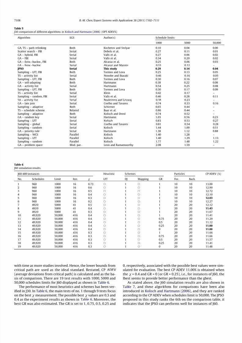
with time as more studies involved. Hence, the lower bounds from

critical path are used as the ideal standard. Restated, CP ADEV

(average deviations from critical path) is calculated and as the ba-

sis of comparison. There are 19 test results with 1000, 5000 and

50,000 schedules limits for J60 displayed as shown in Table 6.

The performance of most heuristics and schemes has been ver-

ified in J30. In Table 6, the main tests of no. 1 through 9 tests focus

on the best v measurement. The possible best v values are 0.3 and

0.4 as the experiment results as shown in Table 6. Moreover, thebest GR was also estimated. The GR is set to 1, 0.75, 0.5, 0.25 and

0, respectively, associated with the possible best values were sim-

ulated for evaluation. The best CP ADEV 11.00% is obtained when

the v = 0.4 and GR = 0 (or GR = 0.25), i.e., for instances of J60, the

lbest seems to provide better performance than the gbest.

As stated above, the J60 simulation results are also shown in

Table 7, and these algorithms for comparisons have been also


according to the CP ADEV when schedules limit is 50,000. The JPSO

proposed in this study ranks the 6th on the comparison table, itindicates that the JPSO can performs well for instances of J60.

Table 5

J30 comparison of different algorithms in Kolisch and Hartmann (2006) (OPT ADEV%)

Algorithm SGS Author(s) Schedule limits

1000 5000 50,000

GA, TS – path relinking Both Kochetov and Stolyar 0.10 0.04 0.00

Scatter search – FBI Serial Debels et al. 0.27 0.11 0.01

GA – hybrid, FBI Serial Valls et al. 0.27 0.06 0.02

GA – FBI Serial Valls et al. 0.34 0.20 0.02

GA – forw.–backw., FBI Both Alcaraz et al. 0.25 0.06 0.03

GA – forw.–backw. Serial Alcaraz and Maroto 0.33 0.12 –

JPSO Serial This study 0.29 0.14 0.04

Sampling – LFT, FBI Both Tormos and Lova 0.25 0.13 0.05

TS – activity list Serial Nonobe and Ibaraki 0.46 0.16 0.05


GA – self-adapting Both Hartmann 0.38 0.22 0.08

GA – activity list Serial Hartmann 0.54 0.25 0.08


TS – activity list Serial Klein 0.42 0.17 –

Sampling – random, FBI Serial Valls et al. 0.46 0.28 0.11

SA – activity list Serial Bouleimen and Lecocq 0.38 0.23 –

GA – late join Serial Coelho and Tavares 0.74 0.33 0.16

Sampling – adaptive Both Schirmer 0.65 0.44 –

TS – schedule scheme Related Baar et al. 0.86 0.44 –

Sampling – adaptive Both Kolisch and Drexl 0.74 0.52 –

GA – random key Serial Hartmann 1.03 0.56 0.23

Sampling – LFT Serial Kolisch 0.83 0.53 0.27Sampling – global Serial Coelho and Tavares 0.81 0.54 0.28

Sampling – random Serial Kolisch 1.44 1.00 0.51

GA – priority rule Serial Hartmann 1.38 1.12 0.88

Sampling – WCS Parallel Kolisch 1.40 1.28 –

Sampling – LFT Parallel Kolisch 1.40 1.29 1.13

Sampling – random Parallel Kolisch 1.77 1.48 1.22

GA – problem space Mod. par. Leon and Ramamoorthy 2.08 1.59 –

Table 6


J60:480 instances Heuristic Schemes Particles CP ADEV (%)

No. Schedules Limit Iter. v LFT DJ Mapping GR For. Back.1 960 1000 16 0.73 s 1 s 1 10 10 13.00

2 960 1000 16 0.6 s 1 s 1 10 10 12.90

3 960 1000 16 0.5 s 1 s 1 10 10 12.72

4 960 1000 16 0.4 s 1 s 1 10 10 12.10

5 960 1000 16 0.3 s 1 s 1 10 10 12.03

6 960 1000 16 0.2 s 1 s 1 10 10 12.27

7 4920 5000 41 0.5 s 1 s 1 20 20 12.12

8 4920 5000 41 0.4 s 1 s 1 20 20 11.43

9 4920 5000 41 0.3 s 1 s 1 20 20 11.67

10 49,920 50,000 416 0.4 s 1 s 1 20 20 11.41

11 49,920 50,000 416 0.4 s 1 s 0.75 20 20 11.29

12 49,920 50,000 416 0.4 s 1 s 0.5 20 20 11.12

13 49,920 50,000 416 0.4 s 1 s 0.25 20 20 11.00

14 49,920 50,000 416 0.4 s 1 s 0 20 20 11.00

15 49,920 50,000 416 0.3 s 1 s 1 20 20 11.66

16 49,920 50,000 416 0.3 s 1 s 0.75 20 20 11.66

17 49,920 50,000 416 0.3 s 1 s 0.5 20 20 11.5718 49,920 50,000 416 0.3 s 1 s 0.25 20 20 11.41

19 49,920 50,000 416 0.3 s 1 s 0 20 20 11.48




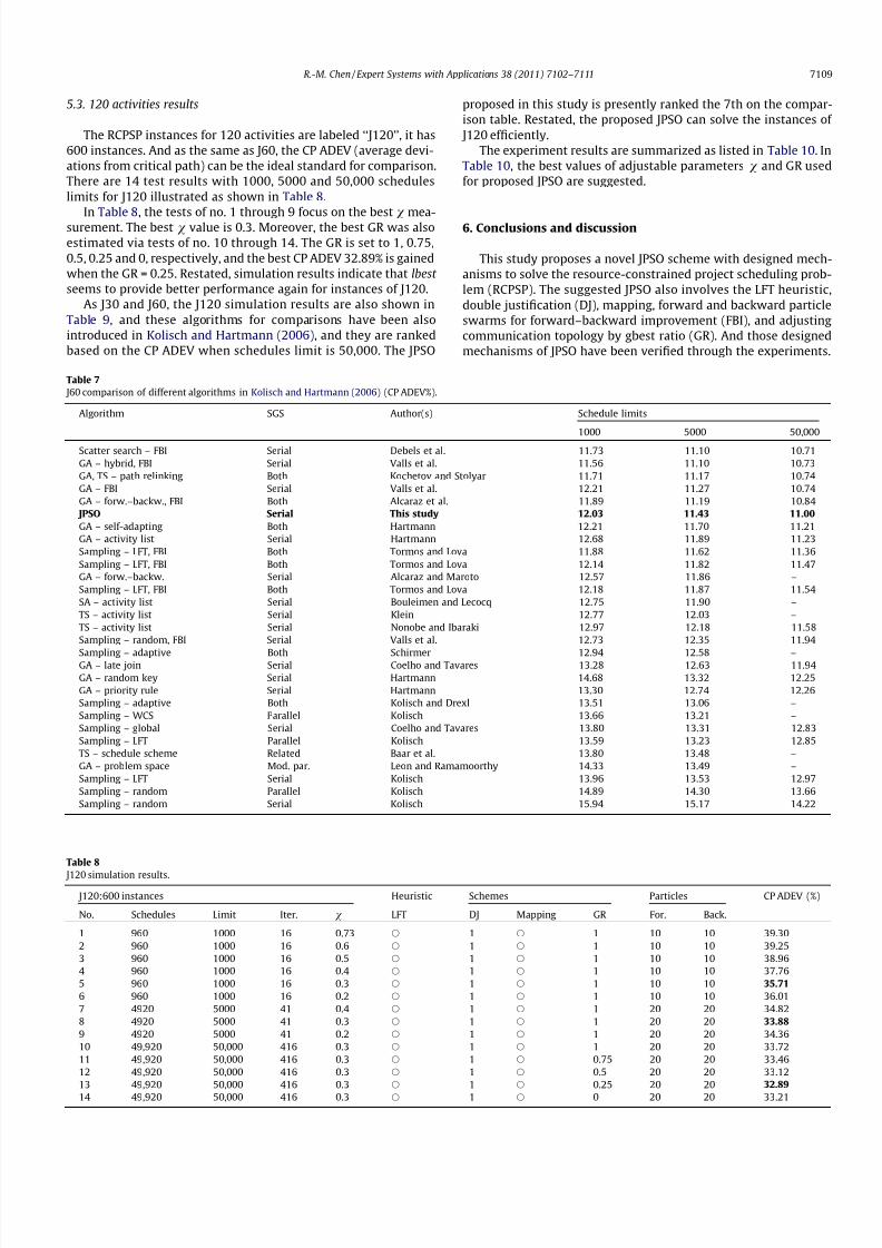
5.3. 120 activities results

The RCPSP instances for 120 activities are labeled ‘‘J120’’, it has

600 instances. And as the same as J60, the CP ADEV (average devi-

ations from critical path) can be the ideal standard for comparison.

There are 14 test results with 1000, 5000 and 50,000 schedules

limits for J120 illustrated as shown in Table 8.

In Table 8, the tests of no. 1 through 9 focus on the bestv mea-surement. The best v value is 0.3. Moreover, the best GR was also

estimated via tests of no. 10 through 14. The GR is set to 1, 0.75,

0.5, 0.25 and 0, respectively, and the best CP ADEV 32.89% is gained

when the GR = 0.25. Restated, simulation results indicate that lbest

seems to provide better performance again for instances of J120.

As J30 and J60, the J120 simulation results are also shown in

Table 9, and these algorithms for comparisons have been also


based on the CP ADEV when schedules limit is 50,000. The JPSO

proposed in this study is presently ranked the 7th on the compar-

ison table. Restated, the proposed JPSO can solve the instances of

J120 efficiently.

The experiment results are summarized as listed in Table 10. In

Table 10, the best values of adjustable parameters v and GR used

for proposed JPSO are suggested.

6. Conclusions and discussion

This study proposes a novel JPSO scheme with designed mech-

anisms to solve the resource-constrained project scheduling prob-

lem (RCPSP). The suggested JPSO also involves the LFT heuristic,

double justification (DJ), mapping, forward and backward particle

swarms for forward–backward improvement (FBI), and adjusting

communication topology by gbest ratio (GR). And those designed

mechanisms of JPSO have been verified through the experiments.

Table 7

J60 comparison of different algorithms in Kolisch and Hartmann (2006) (CP ADEV%).


1000 5000 50,000Scatter search – FBI Serial Debels et al. 11.73 11.10 10.71













TS – activity list Serial Klein 12.77 12.03 –



Sampling – adaptive Both Schirmer 12.94 12.58 –GA – late join Serial Coelho and Tavares 13.28 12.63 11.94

GA – random key Serial Hartmann 14.68 13.32 12.25



Sampling – WCS Parallel Kolisch 13.66 13.21 –

Sampling – global Serial Coelho and Tavares 13.80 13.31 12.83


TS – schedule scheme Related Baar et al. 13.80 13.48 –


Sampling – LFT Serial Kolisch 13.96 13.53 12.97



Table 8


J120:600 instances Heuristic Schemes Particles CP ADEV (%)

No. Schedules Limit Iter. v LFT DJ Mapping GR For. Back.

1 960 1000 16 0.73 s 1 s 1 10 10 39.30

2 960 1000 16 0.6 s 1 s 1 10 10 39.25

3 960 1000 16 0.5 s 1 s 1 10 10 38.96

4 960 1000 16 0.4 s 1 s 1 10 10 37.76

5 960 1000 16 0.3 s 1 s 1 10 10 35.71

6 960 1000 16 0.2 s 1 s 1 10 10 36.01

7 4920 5000 41 0.4 s 1 s 1 20 20 34.82

8 4920 5000 41 0.3 s 1 s 1 20 20 33.88

9 4920 5000 41 0.2 s 1 s 1 20 20 34.36

10 49,920 50,000 416 0.3 s 1 s 1 20 20 33.72

11 49,920 50,000 416 0.3 s 1 s 0.75 20 20 33.46

12 49,920 50,000 416 0.3 s 1 s 0.5 20 20 33.12

13 49,920 50,000 416 0.3 s 1 s 0.25 20 20 32.89

14 49,920 50,000 416 0.3 s 1 s 0 20 20 33.21




The resulting ADEV is decreased after applying those schemes as

indicated in the experiment results. Additionally, the resulting

OPT ADEV and CP ADEV by applying JPSO are also compared with

the top state-of-art algorithms (Kolisch & Hartmann, 2006).

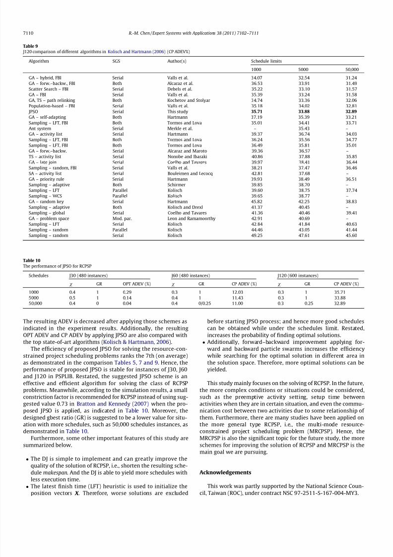
The efficiency of proposed JPSO for solving the resource-con-

strained project scheduling problems ranks the 7th (on average)

as demonstrated in the comparison Tables 5, 7 and 9. Hence, the

performance of proposed JPSO is stable for instances of J30, J60

and J120 in PSPLIB. Restated, the suggested JPSO scheme is an

effective and efficient algorithm for solving the class of RCPSP

problems. Meanwhile, according to the simulation results, a smallconstriction factor is recommended for RCPSP instead of using sug-

gested value 0.73 in Bratton and Kennedy (2007) when the pro-

posed JPSO is applied, as indicated in Table 10. Moreover, the

designed gbest ratio (GR) is suggested to be a lower value for situ-

ation with more schedules, such as 50,000 schedules instances, as

demonstrated in Table 10.

Furthermore, some other important features of this study are

summarized below.

The DJ is simple to implement and can greatly improve the

quality of the solution of RCPSP, i.e., shorten the resulting sche-

dule makespan. And the DJ is able to yield more schedules with

less execution time.

The latest finish time (LFT) heuristic is used to initialize theposition vectors X . Therefore, worse solutions are excluded

before starting JPSO process; and hence more good schedules

can be obtained while under the schedules limit. Restated,

increases the probability of finding optimal solutions.

Additionally, forward–backward improvement applying for-

ward and backward particle swarms increases the efficiency

while searching for the optimal solution in different area in

the solution space. Therefore, more optimal solutions can be

yielded.

This study mainly focuses on the solving of RCPSP. In the future,

the more complex conditions or situations could be considered,such as the preemptive activity setting, setup time between

activities when they are in certain situation, and even the commu-

nication cost between two activities due to some relationship of

them. Furthermore, there are many studies have been applied on

the more general type RCPSP, i.e., the multi-mode resource-

constrained project scheduling problem (MRCPSP). Hence, the

MRCPSP is also the significant topic for the future study, the more

schemes for improving the solution of RCPSP and MRCPSP is the

main goal we are pursuing.

Acknowledgements

This work was partly supported by the National Science Coun-cil, Taiwan (ROC), under contract NSC 97-2511-S-167-004-MY3.

Table 9

J120 comparison of different algorithms in Kolisch and Hartmann (2006) (CP ADEV%)


1000 5000 50,000



Scatter Search – FBI Serial Debels et al. 35.22 33.10 31.57



Population-based – FBI Serial Valls et al. 35.18 34.02 32.81




Ant system Serial Merkle et al. – 35.43 –






GA – late join Serial Coelho and Tavares 39.97 38.41 36.44




Sampling – adaptive Both Schirmer 39.85 38.70 –


Sampling – WCS Parallel Kolisch 39.65 38.77 –GA – random key Serial Hartmann 45.82 42.25 38.83


Sampling – global Serial Coelho and Tavares 41.36 40.46 39.41


Sampling – LFT Serial Kolisch 42.84 41.84 40.63



Table 10

The performance of JPSO for RCPSP

Schedules J30 (480 instances) J60 (480 instances) J120 (600 instances)

v GR OPT ADEV (%) v GR CP ADEV (%) v GR CP ADEV (%)

1000 0.4 1 0.29 0.3 1 12.03 0.3 1 35.715000 0.5 1 0.14 0.4 1 11.43 0.3 1 33.88

50,000 0.4 0 0.04 0.4 0/0.25 11.00 0.3 0.25 32.89




References

Blazewicz, J., Lenstra, J. K., & Rinooy Kan, A. H. G. (1983). Scheduling subject toresource constraints: Classification and complexity. Discrete AppliedMathematics, 5, 11–24.

Bouleimen, K., & Lecocq, H. (2003). A new efficient simulated annealing algorithmfor the resource-constrained project scheduling problem and its multiple modeversions. European Journal of Operational Research, 140(2), 268–281.

Bratton, D., & Kennedy, J. (2007). Defining a standard for particle swarm

optimization. In 2007 IEEE swarm intelligence symposium, SIS 2007 (pp. 120–127).Brucker, P., Knust, S., Schoo, A., & Thiele, O. (1998). A branch and bound algorithm

for the resource-constrained project scheduling problem. European Journal of Operational Research, 107 , 272–288.

Buddhakulsomsiri, J., & Kim, D. S. (2007). Priority rule-based heuristic for multi-mode resource-constrained project scheduling problems with resourcevacations and activity splitting. European Journal of Operational Research, 178,374–390.

Chen, T., Zhang, B., Hao, X., & Dai, Y. (2006). Task scheduling in grid based on particleswarm optimization. In The 5th international symposium on parallel anddistributed computing, 2006 (ISPDC ‘06) (pp. 238–245).

Dorigo, M., & Gambardella, L. M. (1997). Ant colony system: A cooperative learningapproach to the traveling salesman problem. IEEE Transactions on EvolutionaryComputation, 1(1), 53–66.

Edward, W. D., & James, H. P. (1975). A comparison of heuristic and optimumsolutions in resource-constrained project scheduling. Management Science,

21(8), 944–955.Glover, F. (1989). Tabu search – Part I. Orsa Journal on Computing, 1(3),

190–206.Glover, F. (1990). Tabu search – Part II. Informs Journal on Computing, 2, 4–32.Hartmann, S. (2002). A self-adapting genetic algorithm for project scheduling under

resource constraints. Naval Research Logistics, 49, 433–448.Hartmann, S., & Kolisch, R. (1999). Heuristic algorithms for solving the resource-

constrained project scheduling problem: Classification and computationalanalysis. In J. Weglarz (Ed.), Project scheduling. Recent models, algorithms andapplications (pp. 147–178). Boston, MA: Kluwer Academic Publishers.

Holland, John H. (1987). Genetic algorithms and classifier systems: Foundations andfuture directions. In Proceedings of the second international conference on genetic algorithms on genetic algorithms and their application (pp. 82–89).

Hou, Z., Zhou, X., & Wang, Y. (2006). An application-oriented on-demand schedulingapproach in the computational grid environment. In The 5th internationalconference on grid and cooperative computing (GCC 2006), pp. 66–70.

Jalilvand, A., Khanmohammadi, S., & Shabaninia, F. (2005). Scheduling of sequence-dependant jobs on parallel multiprocessor systems using a branch and bound-based Petri net. Emerging technologies. In Proceedings of the IEEE symposium(pp. 334–339).

Kennedy, J., & Eberhart, R. (1995). Particle swarm optimization. In IEEE internationalconference on neural networks, 1995. Proceedings (Vol. 4, pp. 1942–1948).

Kirkpatrick, S., Gelatt, C. D., Jr., & Vecchi, M. P. (1983). Optimization by simulatedannealing. Science, 220(4598), 671–680.

Kolisch, R., & Hartmann, S. (2006). Experimental investigation of heuristics forresource-constrained project scheduling: An update. European Journal of Operational Research, 174, 23–37.

Kolisch, R., & Sprecher, A. (1997). PSPLIB – A project scheduling problem library: OR software – ORSEP operations research software exchange program. European

Journal of Operational Research, 96 , 205–216.Li, C., & Bettati, R., & Zhao, W. (1997). Static priority scheduling for ATM networks.

In 18th IEEE real-time systems symposium (RTSS ‘97 ) (pp. 264–273).Li, K. Y., & Willis, R. J. (1992). An iterative scheduling technique for resource-

constrained project scheduling. European Journal of Operational Research, 56 ,370–379.

Liu, Z., & Wang, S. (2006). Hybrid particle swarm optimization for permutation flowshop scheduling. In The 6th world congress on intelligent control and automation,

2006. WCICA 2006 (pp. 3245–3249).Liu, L., Yang, Y., Shi, W., Lin, W., & Li, L. (2005). A dynamic clustering heuristic for

jobs scheduling on grid computing systems. In First international conference onsemantics, knowledge and grid (SKG ‘05).

Lo, S. T., Chen, R. M., Huang, Y. M., & Wu, C. L. (2008). Multiprocessor systemscheduling with precedence and resource constraints using an enhanced antcolony system. Expert Systems with Applications, 34(3), 2071–2081.

Merkle, D., Middendorf, M., & Schmeck, H. (2002). Ant colony optimization forresource-constrained project scheduling. IEEE Transactions on EvolutionaryComputation, 6 , 333–346.

Ohki, M., Morimoto, A., & Miyake, K. (2008). Simulated annealing algorithm forscheduling problem in daily nursing cares. In 2008 IEEE international conferenceon systems, man and cybernetics (pp. 1681–1687).

Park, H. S., Kim, H. O., Kim, D. S., & Kwon, W. H. (2002). A scheduling method fornetwork-based control systems. IEEE Transactions on Control Systems Technology,10(3), 318–330.

Rutenbar, R. A. (1989). Simulated annealing algorithms: An overview. Circuits andDevices Magazine, IEEE, 5, 19–26.

Saksornchai, T., Lee, W., Methaprayoon, K., Liao, J. R., & Ross, R. J. (2005). Improvethe unit commitment scheduling by using the neural-network-based short-term load forecasting. IIEEE Transactions on Industry Applications, 41(1),169–179.

Simonov, S., & Simonovov’a, J. (2002). Simulation scheduling in food industryapplication. Czech Journal on Food Science, 20(1), 31–37.

Symington, K. J., Waddie, A. J., Taghizadeh, M. R., & Snowdon, J. F. (2003). A neural-network packet switch controller: Scalability, performance, and networkoptimization. IEEE Transactions on Neural Networks, 14(1), 28–34.

Thomas, P. R., & Salhi, S. (1998). A tabu search approach for the resource constrainedproject scheduling problem. Journal of Heuristics, 4(2), 123–139.

Valls, V., Ballest, F., & Quintanilla, S. (2005). Justification and RCPSP: A techniquethat pays. European Journal of Operational Research, 165, 375–386.

Valls, V., Ballest, F., & Quintanilla, S. (2008). A hybrid genetic algorithm for theresource-constrained project scheduling problem. European Journal of Operational Research, 185(2), 495–508.

Vejzovic, Z., & Humo, E. (2007). A software solution for a mathematical model of classroom-period schedule defragmentation. EUROCON: The InternationalConference on Computer as a Tool, 2034–2038.

Zhang, H., Li, H., & Tam, C. M. (2006). Particle swarm optimization for resource-constrained project scheduling. International Journal of Project Management,

24(1), 83–92.Zhang, C., Sun, J., Zhu, X., & Yang, Q. (2008). An improved particle swarm

optimization algorithm for flowshop scheduling problem. InformationProcessing Letters, 108(4), 204–209.


TOPOLOGIA VECINOS 1-s2.0-S0957417410014223-main

Documents

Transcript of TOPOLOGIA VECINOS 1-s2.0-S0957417410014223-main