18

Vol. 11, No.1, 18–35 6 de abril de 2018

REVISTA AIDIS de Ingeniería y Ciencias Ambientales: Investigación, desarrollo y práctica. MOC−BASED SECOND−ORDER EXPLICIT SCHEME FOR WATER HAMMER ANALYSIS

*John Twyman Q1

MÉTODO DE LAS CARACTERÍSTICAS DE 2° ORDEN PARA EL ANÁLISIS DEL GOLPE DE ARIETE Recibido el 30 de junio de 2016; Aceptado el 20 de noviembre de 2017 Abstract Method of Characteristics (MOC) needs to fulfil the Courant condition (Cn = 1.0) in order to guarantee the stability and convergence on the results. Otherwise, whenever Cn < 1.0 is necessary to apply interpolation processes to calculate the state variables Q and H at the discretization nodes. In many cases, the application of MOC with first-order accuracy is more convenient due to its minor complexity, even if its principal disadvantage is the introduction of significant numerical attenuation as Cn value decreases away from 1.0, being necessary to have numerical schemes with higher accuracy in these cases. This paper introduces a MOC-based second-order explicit scheme useful to solve the transient flow when Courant is different from 1.0. It verifies that MOC 2nd-order is more accuracy than MOC 1st-order in a wide range of Courant numbers, even when Cn > 1.0, where with the help of numerical filters or artificial viscosities MOC can continue to function without to affect its accuracy or numerical stability. This feature allows get a greater time step which helps to reduce significantly the computation time. Keywords: interpolation scheme, Method of Characteristics, numerical oscillations, order of interpolation, water hammer. 1 Twyman Ingenieros Consultores, Chile. *Autor corresponsal: Pasaje Dos No. 362, Rancagua Norte, Rancagua, VI Región, Chile. Email: john@twyman.cl

19

Vol. 11, No.1, 18–35 6 de abril de 2018

Resumen El Método de las Características (MC) necesita cumplir la condición de Courant (Cn = 1,0) para garantizar la estabilidad y convergencia en los resultados. De lo contrario, siempre que Cn < 1,0 es necesario aplicar un procedimiento de interpolación para calcular las variables de estado Q y H en los nodos de la discretización. En muchos casos, la aplicación del MC con una precisión de primer orden es más conveniente debido a su menor complejidad, aunque su principal desventaja es la introducción de atenuaciones numéricas significativas a medida que Cn disminuye alejándose de 1,0, siendo necesario en estos casos contar con esquemas numéricos con mayor nivel de precisión. Este trabajo presenta un esquema explícito de 2do orden basado en el MC útil para resolver el golpe de ariete cuando Courant es diferente de 1,0. Se verifica que el MC de 2do orden es más preciso que el MC de 1er orden dentro de un rango amplio de Cn, incluso considerando valores de Cn > 1.0, donde con la ayuda de filtros numéricos o viscosidades artificiales el MC puede seguir funcionando sin perder estabilidad ni precisión numérica. Esta característica permite obtener un intervalo de tiempo mayor que ayuda a reducir significativamente el tiempo de cálculo. Palabras clave: esquema de interpolación, golpe de ariete, método de las características, orden de interpolación, oscilaciones numéricas. Introduction Interpolation is required in many engineering applications that use tabular data as input. The basis of all interpolation is the fit of some type of curve or function into a subset of the tabular data. Generally we know the value of the function f (x) at a set of points, but we do not have an analytic expression for f (x) that enables us calculating its value at any arbitrary point. Always it is better to develop the function f (x) directly from N tabulated values, even though the erroneous selection of interpolation scheme or the inadequate choice of the order of interpolation (i.e., number of points minus one used in the interpolation procedure) can lead to incorrect results of f (x). In many cases the increment of such order does not necessarily means an increment of the accuracy, especially in polynomial interpolation. Unless there is solid evidence that the interpolating function is close to the true function, it is necessary to be cautious about high-order interpolation (Press et al., 1986). In the context of the Method of Characteristics (MOC) with pre-specified time intervals it is necessary to reach a common time step (∆t) for the entire network. This restriction makes difficult to fulfil with the Courant condition (Cn = 1.0) because the system may have a diversity of pipe lengths and wave speeds. In this case, it is preferable to apply a numerical interpolation on the x-t grid instead of attempting to comply with Cn = 1.0 by changing any initial condition such as the pipe length or wave speed, due to may alter the physics of the problem (Ghidaoui et al., 1998, Twyman, 2016b), although the interpolation can introduce significant numerical attenuation that smoothing the sharp pressure front which actually happens (Streeter, 1972). Despite this fact, the incorporation of high-order interpolation schemes makes it possible to get reasonable results in accuracy without increasing greatly the model complexity.

20

Vol. 11, No.1, 18–35 6 de abril de 2018

There exist a large number of numerical techniques aimed to deal with the polynomial interpolation based on finding a polynomial which fits through the given points, highlighting the Newton-Gregory (NG) method (Twyman, 2018). In the next paragraphs, original analytical expressions for the NG method will be described within the MOC context (with first and second-order accuracy). The first (1st) and second (2nd) order polynomial interpolation will be applied in order to learn about their main characteristics and performance whenever is necessary to interpolate on the x-t grid with Cn < 1.0, and when also is necessary to solve the water hammer in x-t grid with Cn > 1.0. In each case the comparison between the results obtained by MOC with NG polynomial interpolation and the exact solution obtained by MOC with Cn = 1.0 will be shown. Method of characteristics (MOC) Well-known MOC is a simple and numerically efficient scheme for solving the unsteady flow equations by converting the non-linear hyperbolic partial differential equations into straight forward ordinary differential equations. The finite difference approach of the ordinary differential equations can be easily implemented in computer programming (Chaudhry, 1979; Watters, 1984, Nerella and Rathnam, 2015; Twyman, 2016a, 2017). MOC combines the momentum and continuity equations to form the following compatibility equation in terms of discharge Q and piezometric head H (Goldberg and Wylie, 1983):

0=∆

±⋅± QQx

RdQBdH f

Equation (1) With H = piezometric head, B = pipe constant, Q = flow rate, R f = frictional term and ∆x = reach length. Equation (1) represents exactly the original system (momentum and continuity equations) along the so-called characteristics lines (i = 2,.…, N): Along positive characteristic line (C+):

[ ] 02 2 =

∆+−+− L

tiL

tiL

ti QQ

gDAxfQQ

gAaHH

Equation (2) Along negative characteristic line (C−):

[ ] 02 2 =

∆−−+− R

tiR

tiR

ti QQ

gDAxfQQ

gAaHH

Equation (3) In which N = number of computational nodes, a = wave speed, g = acceleration due to gravity, t = time, ∆t = computational time step, f = friction factor, D = pipe diameter, and i = node number.

21

Vol. 11, No.1, 18–35 6 de abril de 2018

Solving tiH and

tiQ from (2) and (3) the following is obtained (Watters, 1984):

−

∆−−++= RRLLRLRL

ti QQQQ

gDAtafQQ

gAaHHH (

2)()(

21

2

Equation (4)

+

∆−++−= RRLLRLRL

ti QQQQ

DAtfQQHH

agAQ (

2)()(

21

Equation (5) Where HL, QL, HR and QR are the state variables at nodes L and R, respectively (see figure 1).

Figure 1. Space-time grid (Δx, Δt) with characteristic lines (C+ and C−). LP = pipe length. At the border sections (1 and N+1) an additional boundary condition is required which must be solved jointly with negative or positive characteristic equation accordingly to the first or last subdivision pipe section, respectively. The stability and convergence of the MOC is guaranteed when the Courant-Friedrichs-Lewy condition (CFL) is fulfilled, that is, when Cn = 1.0 or when (a ∙ ∆t) = ∆x (Goldberg and Wylie, 1983). Otherwise, when Cn < 1.0 it is necessary apply an interpolation process in order to calculate H and Q at the grid nodes, with risk of generating numerical attenuations which do not correspond to a physical reality (Chaudhry and Hussaini, 1985; Contin and Cardim, 1994). There are not too many techniques to deal with the task of calculating the state variables at nodes L and R, even though some authors have presented alternative original algorithms which are based upon well-known interpolation methods

C+ C–

P

∆t

∆x

Time t

Distance x

≈

≈ ≈ ≈

i–1 i+1it

t + ∆t ≈

1 N+1≈

≈

LP

L R i+2i–2

22

Vol. 11, No.1, 18–35 6 de abril de 2018

(Goldberg and Wylie, 1983; Watters, 1984; Sibetheros et al., 1991; Karney and McInnis, 1992; Karney and Ghidaoui, 1997). In the MOC context, several analytical expressions for state variables at nodes L and R can be obtained starting by different interpolation schemes and/or interpolation order, usually one (linear) or two (quadratic). In the following paragraphs original analytical expressions for calculation of the state variables at nodes L and R using MOC with Newton-Gregory interpolation method (first and second-order) will be shown. Theory related to this interpolation scheme and deduction of analytical expressions will not be included in this paper due to space restrictions. Polynomial interpolation A polynomial is a mathematical expression comprising a sum of terms, each term including a variable or variables raised to a power and multiplied by a coefficient. When graphical data contains a gap, but data is available on either side of the gap or at a few specific points within the gap, an estimate of values within the gap can be made by interpolation. Thus, the polynomial interpolation is a method of estimating values between known data points. The simplest method of interpolation is to draw straight lines between the known data points and consider the function as the combination of those straight lines. This method, called linear interpolation, usually introduces considerable error. A more accurate approach uses a polynomial function to connect the points. If a set of data contains n known points, then there exists exactly one polynomial of order n−1 or smaller that passes through all of those points. This methodology, known as polynomial interpolation, often (but not always) provides more accurate results than linear interpolation. Newton-Gregory interpolation scheme Rather than defining a set of functions for a given set of points, Newton-Gregory method takes things one point at a time. Because it is an interpolation method based upon the Taylor series, the unique polynomial satisfying any n+1 values of degree n is (Gerald and Wheatley, 1984):

nntUtUtUUU ++++= .....2

210 Equation (6) The n+1 constants Ui being found from the n+1 linear equations obtained by substituting in the data. Suppose the n+1 values are (ti, Ui), i = 0, 1, 2,...., n, and suppose that equal intervals between successive values is h, then tr – ts = (r – s) ‧ h. Forming successive differences and taking into account that (t – t0) = k ‧ h, with 0 ≤ k ≤ n, then:

!)1)...(1(.....

!2)1( 00

2

00 nU

nkkkU

kkUkUUN∆

+−−++∆

−+∆+= Equation (7)

23

Vol. 11, No.1, 18–35 6 de abril de 2018

Equation (7) is known as the forward interpolation formula and it is appropriate when the required value (t, U) lies near the beginning of the tabulated data; otherwise, when the value (t, U) is near the end of the table, it is necessary to apply the backward interpolation formula. Newton-Gregory does not need to solve a set of simultaneous equations and it works very well with equally spaced data points, where the best accuracy is usually achieved when the differences in the spacing of the data points are minimal. In the Newton-Gregory context is possible to derive the following analytical formulas for UL and UR at time t (i = 2,......, N) (Twyman, 2004, 2016a): First−order arrangement (linear):

nti

ti

tiL CUUUU ⋅−+= −−

−− )( 11

11

Equation (8) n

ti

ti

tiR CUUUU ⋅−+= −−

+− )( 11

11

Equation (9) Second−order arrangement (quadratic):

)()2(21)( 211

112

111

1nn

ti

ti

tin

ti

ti

tiL CCUUUCUUUU −⋅+−−⋅−+= −−

−−−

−−−

−

Equation (10)

)()2(21)( 211

112

111

1nn

ti

ti

tin

ti

ti

tiR CCUUUCUUUU −⋅+−−⋅−+= −−

+−+

−−+

−

Equation (11) In which U is used instead H and Q for brevity. In the second-order arrangement the values for

tU 0 and tNU 2+ can be calculated through the application of an extrapolation procedure defined by

the following formulas (Chaudhry and Hussaini, 1985; Twyman, 2004):

ttt UUU 210 2 −= Equation (12) tN

tN

tN UUU −= ++ 12 2 Equation (13)

In which tU 0 and

tNU 2+ are the corresponding values located upstream of the left border node

and downstream of the right border node at time t, respectively. Once known UL and UR, it is

possible to calculate tiH and

tiQ from equations (4) and (5), respectively.

Simple one-node boundary condition According to Karney and McInnis (1992), one the most important boundary condition is the multi-pipe frictionless junction, where the concept “frictionless” is equivalent to saying that the hydraulic grade line (HGL) elevation at the node can be represented by a single number, designed HP (Twyman, 2016a, 2017):

24

Vol. 11, No.1, 18–35 6 de abril de 2018

extcctt

P QBCH ⋅−=∆+

Equation (14) With t = current simulation time, ∆t = time step, Cc and Bc = known constants and Qext = external flow that may be constant or a function of time, and where the sign convention is that positive flows are directed away from the junction being considered. Equation (14) represents the general multi-pipe junction with one external flow which it allows a simple treatment of networks with complex topology (Wylie, 1986), and it also allows to decouple the pipelines of complex networks in each node, restoring the flow continuity and the HGL in the node. This feature simplifies the treatment of the connectivity in simple and complex pipe networks. Valve boundary condition If flow passes into a reservoir through a restriction, a general loss and storage expression may be derived, which it can be used to represent valves or orifices discharging to linear reservoirs or to atmosphere. The external flow is related to the head at the junction by the orifice expression (Karney and McInnis, 1992):

( )cPPsext HHsEsQ −⋅⋅⋅⋅= τ Equation (15)

In which s = sign of the external flow [i.e., s = sign (Qext) = ±1] and

cPH = head at the node side of

the connector. The terms τ and Es in (15) are valve or orifice parameters; by convention, τ = 1.0 implies a fully open valve, while a value of zero requires the valve to be closed. Opening and closing valves can be represented if τ is a function of time. The valve scaling constant Es represents two values: E+ for flow from the network when s = +1.0 and E− for negative flow. The values of these terms are determined by knowing HP,

cPH , τ and Qext for one positive and one negative flow

(further details in Karney and McInnis, 1992). Example of application 1 Water hammer in the simple pipeline system of figure 2 is analyzed, which it comprises one reservoir (upstream), one steel pipe and a valve (downstream). The pipe length is L = 4,800 (m), wave speed a = 1,200 (m/s), pipe cross-sectional area A = 3.14 (m2), initial steady-state flow Q0 = 2.63 (m3/s) and H0 = 100 (m). The computational time step is ∆t = 0.4 (s). The transient flow condition is generated by the valve closure in Tc = 35 s (see relative valve opening in the figure 3), in which τ = Cd ‧Av ‧ (2g ‧ H0)1/2 ‧ Q0−1 is an adimensional parameter where Cd = valve discharge coefficient, Av = opening valve area, H0 = initial piezometric head at the valve, and Q0 = initial flow at the valve. The curve which describes the valve closure will be interpolated using the Newton-Gregory method with order of interpolation equal to 7.

25

Vol. 11, No.1, 18–35 6 de abril de 2018

This condition allows reduce to the maximum the spurious oscillations which can appear when the valve closure curve is being interpolated (Twyman, 2018). According to the traditional criterion, usually a comparison between the valve motion to the wave travel time in pipe system is adopted in order to determinate if the valve motion is rapid or slow (Jung and Karney, 2016; Kodura, 2016). In this case, the transient flow can be considered as “slow” because the relation 2 ‧ (L / a) = 8 (s) is much lower than Tc. For all purposes the exact result is given by MOC (1st or 2nd-order) with Cn = 1.0. Figures 4 and 5 show the extreme pressure heads obtained by MOC (1st and 2nd-order, respectively) when the pipe is discretized so as to obtain different Courant numbers: 0.2 (∆x = 2,400 m), 0.4 (∆x = 1,200 m), 0.6 (∆x = 800 m), 0.8 (∆x = 600 m) and 1.0 (∆x = 480 m).

Figure 2. Pipe network example (adapted from Wylie and Streeter, 1978).

Figure 3. Relative valve opening τ (Tau = τ).

H0 = 100

Reservoir

1 2

Pipe Valve

0.00.10.20.30.40.50.60.70.80.91.0

0 10 20 30 40

Tau

Time (s)

26

Vol. 11, No.1, 18–35 6 de abril de 2018

Figure 4. Envelope of extreme pressure heads for different Courant numbers (MOC 1st-order).

Figure 5. Envelope of extreme pressure heads for different Courant numbers (MOC 2nd-order). With MOC (1st-order) the maximum pressure head shows attenuations which it decreases as the Courant number grows towards the critical value Cn = 1.0 (figure 4). Figure 5 shows that MOC (2nd-order) also it generates attenuations but smaller compared to the MOC 1st-order case. Error of the maximum pressure head according to MOC 1st-order and MOC 2nd-order is shown in table 1, where the error obtained by MOC (2nd-order) when Cn = 0.2 is much lower than the error obtained by MOC (1st-order) when Cn = 0.8, value which is closer to the critical value 1.0. It is verified in this case that MOC (2nd-order) is more accurate than the MOC (1st-order) in a wide range of values Cn (less than 1.0), as it is shown in Table 1. Table 2 shows the execution time for each case analyzed when the software was carried out in a standard PC with CPU @ 1.66 GHz. It can verify that MOC (2nd-order) is slower than the MOC (1st-order), especially when Cn is much less than 1.0, even though the gap in runtime between the two methods is reduced as Cn grows, and it is almost equalized when Cn = 1.0.

60

90

120

150

180

0 1 2 3 4 5Distance (km)

Hea

d (m

)

Cn = 0.2 Cn = 0.4 Cn = 0.6

Cn = 0.8 Cn = 1.0

60

90

120

150

180

0 1 2 3 4 5Distance (km)

Hea

d (m

)

Cn = 0.2 Cn = 0.4 Cn = 0.6

Cn = 0.8 Cn = 1.0

27

Vol. 11, No.1, 18–35 6 de abril de 2018

Table 1. Error in maximum pressure head (MOC 1st and 2nd-order).

MOC 1st order

Cn 0.2 0.4 0.6 0.8 1.0

Error in max. pressure head (m) −7.2 −6.1 −4.7 −3.1 0.0

MOC 2nd order

Cn 0.2 0.4 0.6 0.8 1.0

Error in max. pressure head (m) −2.7 −2.3 −1.8 −1.4 0.0

Table 2. Runtime according to different Courant numbers (MOC 1st and 2nd-order).

MOC 1st order

Cn 0.2 0.4 0.6 0.8 1.0

Runtime (s) 0.88 0.38 0.27 0.16 0.16

MOC 2nd order

Cn 0.2 0.4 0.6 0.8 1.0

Runtime (s) 1.15 0.44 0.33 0.27 0.17

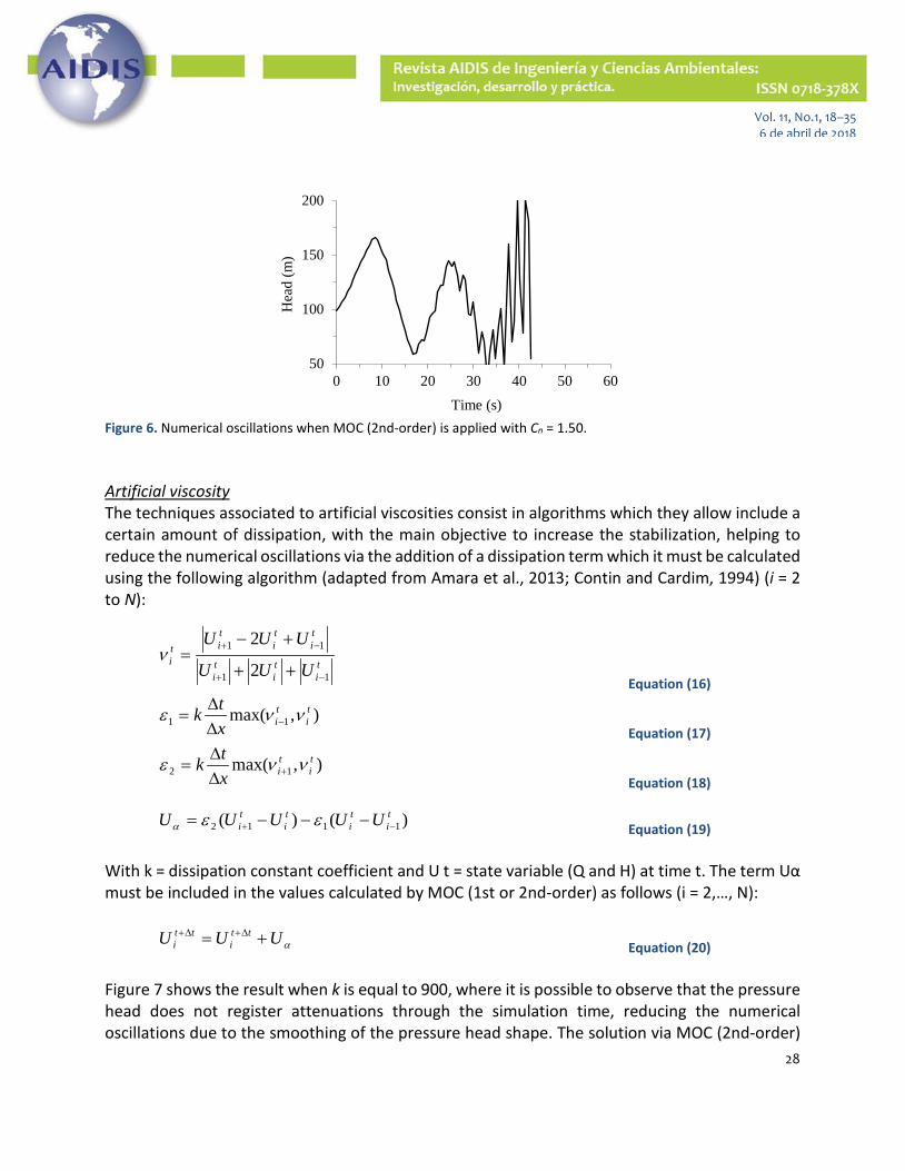
Numerical oscillations It is important to take into account that even though linear stability analysis may confirm the stability of an explicit numerical scheme, instability may still occur in highly nonlinear cases involving shocks. Capturing all features of the discontinuity is practically impossible and there exist some scales of motion that cannot be resolved numerically (Malekpour and Karney, 2015). Different alternatives to reduce the typical non-physical numerical oscillations which appear during the transient flow are shown below. In general, the oscillations appear when Cn > 1.0 regardless of the order (1st or 2nd) chosen for MOC. For example, figure 6 shows the pressure head vs. time plot when the system shown in figure 2 is discretized such that Cn = 1.50 (∆t = 0.6 s, ∆x = 480 m), and MOC 2nd-order is applied. As it is expected, spurious numerical oscillations appear which grow as the simulation time progresses. There are many dissipation techniques to deal with this problem, like the inclusion of an artificial viscosity or the application of the dissipative interface (see details below). Additional options based on modifying the mesh x-t (∆x, ∆t) (Contin and Cardim, 1994) or N (Chaudhry and Hussaini, 1985), wave-speed adjustments (Wylie, 1978, Karney and McInnis, 1992, Twyman 2016b) to get Cn = 1.0, or the application of hybrid methods (Twyman, 2004, 2017) will not be discussed here because these methodologies can modify some of the initial data and the idea of the present analysis is to maintain constant Cn = 1.5.

28

Vol. 11, No.1, 18–35 6 de abril de 2018

Figure 6. Numerical oscillations when MOC (2nd-order) is applied with Cn = 1.50. Artificial viscosity The techniques associated to artificial viscosities consist in algorithms which they allow include a certain amount of dissipation, with the main objective to increase the stabilization, helping to reduce the numerical oscillations via the addition of a dissipation term which it must be calculated using the following algorithm (adapted from Amara et al., 2013; Contin and Cardim, 1994) (i = 2 to N):

ti

ti

ti

ti

ti

tit

i UUU

UUU

11

11

2

2

−+

−+

++

+−=ν

Equation (16)

),max( 11ti

tix

tk ννε −∆∆

= Equation (17)

),max( 12ti

tix

tk ννε +∆∆

= Equation (18)

)()( 1112ti

ti

ti

ti UUUUU −+ −−−= εεα Equation (19)

With k = dissipation constant coefficient and U t = state variable (Q and H) at time t. The term Uα must be included in the values calculated by MOC (1st or 2nd-order) as follows (i = 2,…, N):

αUUU tti

tti += ∆+∆+

Equation (20) Figure 7 shows the result when k is equal to 900, where it is possible to observe that the pressure head does not register attenuations through the simulation time, reducing the numerical oscillations due to the smoothing of the pressure head shape. The solution via MOC (2nd-order)

50

100

150

200

0 10 20 30 40 50 60

Hea

d (m

)

Time (s)

29

Vol. 11, No.1, 18–35 6 de abril de 2018

with artificial viscosity is closer to the exact solution during the period of duration of the simulation, with a slight displacement of the pressure head curve as the simulation time progresses, without losing its shape.

Figure 7. MOC 2nd-order (Cn = 1.50 and artificial viscosity k = 900). Dissipative interface In this case, the state variables are recalculated every two time steps as it follows using a dissipation constant term (γ) as a weighting factor (Abbott and Basco, 1989) (i = 2,….,N):

ti

ti

ti

tti UUUU 11 )21( −+

∆+ ⋅+⋅⋅−+⋅= γγγ Equation (21) Figure 8 shows that numerical oscillations disappear when γ = 0.10. In this particular case the solution is more conservative because the extreme pressure heads are slightly greater than those reached with MOC (1st-order, Cn = 1.0), and the displacement of the pressure head curve is negligible as the simulation time progresses, without losing its shape.

Figure 8. MOC 2nd-order (Cn = 1.50 and dissipative interface γ = 0.10).

50

100

150

200

0 10 20 30 40 50 60

Hea

d (m

)

Time (s)

50

100

150

200

0 10 20 30 40 50 60

Hea

d (m

)

Time (s)

30

Vol. 11, No.1, 18–35 6 de abril de 2018

In general, the application of the dissipative interface or artificial viscosity is recommendable due to their simplicity although its main disadvantage is that dissipative coefficients (k or γ) are difficult to estimate, being necessary a trial and error procedure before getting suitable values. For example, in the case of the artificial viscosity, table 3 shows the iterative values tested to reach a maximum pressure head near the exact value (H max = 165.2 m), where it is observed that in this particular case k has a range of applicability between k > 50 and k < 1,000, with optimum value of k = 900. In table 3 the symbol “*” in the last column indicates that the simulation was stopped because of a false effect of water column separation. In the case of the dissipative interface, table 4 shows the iterative values which have tested with the objective to reach a maximum pressure head nearest the exact value, where the value 0.10 is critical because when γ < 0.10, the dissipative interface generates a maximum which far exceeds the exact value. Otherwise, when γ is increased in values greater than 0.10, significant attenuation is generated in relation with the exact value. In this case the dissipative interface generates a more conservative solution because the pressure head (maximum and minimum) slightly exceed the exact value (MOC 1st-order) as the simulation time progresses. Table 3. Error for different k values.

k Max. Pressure Head (m)

Error (%)

50 184.2 +11.5 *

200 166.1 +0.5

400 165.9 +0.4

900 165.7 +0.3

1,000 165.8 +0.4 *

Table 4. Error for different γ values.

γ Max. Pressure Head (m)

Error (%)

0.04 223.8 +35.5

0.10 164.9 −0.2

0.20 163.8 −0.8

0.30 162.9 −1.4

0.40 162.1 −1.9

31

Vol. 11, No.1, 18–35 6 de abril de 2018

Fast transient flow It is convenient to analyze the numerical performance of the MOC (2nd-order) when it is required to simulate a fast transient flow. The idea is to detect the occurrence (or not) of spurious numerical oscillations that commonly appear in these cases when a 2nd-order scheme is applied, such as it has been reported by some authors (Amara et al., 2013; Chaudhry and Hussaini, 1985; Sibetheros et al., 1991; Contin and Cardim, 1994; Twyman, 2004). For this purpose, it is considered that the valve included in the system of figure 2 closes in 1 (s). The transient flow is considered as “fast” because the relation 2 ‧ L / a = 8 (s) is much greater than Tc. The results between MOC (1st and 2nd-order) and McCormack (2nd-order) are compared. The McCormack method will not be described here due to space restrictions, although more details can be found in Chaudhry and Hussaini (1985), or in a recent paper by Twyman (2017). Figure 9 shows the errors of MOC (2nd-order) and McCormack (2nd-order) in comparison with the exact solution (MOC 1st-order with Cn = 1.0). In each case the error is calculated using the following expression:

E(t) = H comp(t) – H exact(t) Equation (22)

With E(t) = error (m) in time t, with t = 0,….,T max, T max = 60 (s) and H comp(t) = computed piezometric head in time t and H exact(t) = exact piezometric head in time t. It can be seen in figure 9 that at the beginning of the transient flow the errors generated by MOC (2nd-order) and McCormack (2nd-order) are almost minimum. However, the first method is maintained at optimal performance, being its error compared with the exact solution almost zero as the simulation time progresses (see solid line in figure 9). Instead, McCormack’s method begins to show an error (E) from time equal to 8.4 (s) that it tends to grow as the simulation time progresses (see dashed line in figure 9).

Figure 9. MOC (2nd-order) and McCormack (2nd-order) error when the valve closes in 1 (s). Cn = 1.0.

-10

-5

0

5

10

15

0 10 20 30 40 50 60

E (m

)

Time (s)

MOC (2nd-order) McCormack (2nd-order)

32

Vol. 11, No.1, 18–35 6 de abril de 2018

Example of application 2 The single pipe apparatus (Bergant et al., 2008) is used for investigating the water hammer wave forms comprises a metal (copper) pipeline of length 37.2 (m), 22 (mm) internal diameter and 1.6 (mm) wall thickness that is upward sloping (figure 10). The transient event is generated by a rapid closure of the downstream end valve. The apparatus is installed in Robin hydraulic laboratory of the Department of Civil and Environmental Engineering at the University of Adelaide (Bergant et al., 2008). The initial flow velocity is V0 = 0.2 (m/s), static head in the tank 2, HT = 32 (m), valve closure time Tc = 0.009 (s), and water hammer wave speed a = 1,319 (m/s). The number of reaches for the computational run is N = 32, and the time step (∆t) = 0.00088135 (s). In this example, the transient flow can be considered as “fast” because the relation 2 ‧ (L / a) = 0.056 (s) is much greater than Tc.

Figure 10. Single pipe apparatus (adapted from Bergant el al., 2008). In this case, and due to space reasons, only will be analyzed the numerical performance of the MOC (2nd-order) when it is required to simulate a very fast transient flow, applying as numerical filter the dissipative interface in case it is necessary in order to attenuate the spurious oscillations. Figures 11 and 12 show the head vs. pressure plot at the valve according to MOC (1st order) and MOC (2nd order) when they are applied with different Courant numbers (Cn = 1 with ∆x = 1.16 m, Cn = 0.78 with ∆x = 1.49 m, and Cn = 0.50 with ∆x = 2.33 m). It can be seen in figures 11 and 12 that the error generated by MOC (2nd-order) always stays closer to the exact solution, maintaining its optimal numerical performance as the simulation time progresses without to register significant attenuations.

Tank 1

Tank 22.03 m

0.0 m

DATUMValve Pipeline

33

Vol. 11, No.1, 18–35 6 de abril de 2018

Figure 11. Pressure at the valve according to MOC (1st order). Term Cn means Courant number.

Figure 12. Pressure at the valve according to MOC (2nd order). γ = 0.03 for Courant = 0.78 and γ = 0.04 for Courant = 0.50. Conclusions In this article, it verifies that the result of the transient analysis in numerical terms depends on at least three factors: (i) type of transient (fast, slow), (ii) how the network is discretized (taking into account a Courant number less than, equal to or greater than 1.0), and (iii) the solution method chosen (MOC 1st and 2nd order, McCormack, etc.) to calculate Q and H at each system node, considering (or not) an interpolation procedure when Courant is less than 1.0. In this sense, the 2nd-order MOC is more stable and accurate than both the traditional 1st-order MOC and the McCormack scheme regardless the adopted Courant number: less or greater than 1.0.

0

10

20

30

40

50

60

0 0.1 0.2 0.3 0.4 0.5 0.6 0.7 0.8 0.9 1

Hea

d (m

)

Time (s)

Cn = 1.00 Cn = 0.78 Cn = 0.50

0

10

20

30

40

50

60

0 0.1 0.2 0.3 0.4 0.5 0.6 0.7 0.8 0.9 1

Hea

d (m

)

Time (s)

Cn = 1.00 Cn = 0.78 Cn = 0.50

34

Vol. 11, No.1, 18–35 6 de abril de 2018

Another positive feature is that the MOC (second order) maintains its accuracy and stability with the numerical filters help (dissipative interface or artificial viscosity) when Cn is different from 1.0, reducing the spurious oscillations impact that usually appear in the second order explicit schemes and that they contaminate the solution with unrealistic values that often terminate the simulation prematurely.On the other hand, it is possible to solve the transient flow using the MOC (1st or 2nd-order) with a time step greater than the optimum through the application of the artificial viscosity or the dissipative interface for controlling the spurious oscillations, which requires the calculation of an additional term or the recalculation of the state variables, all of which can lead to the application of a time consuming trial/error procedure. Nevertheless, a relevant advantage of these dissipative schemes is that they may significantly help to reduce or even eliminate the numerical instability when MOC (1st or 2nd-order) is applied with Cn > 1.0, without the necessity of modifying some initial data as wave speeds, pipe lengths or the number of the discretization nodes. Besides, this feature may be useful when it is necessary to apply these dissipative techniques for solving the water hammer in pipe networks with hundreds or thousands of pipes, being necessary to count with a greater time step in order to reduce the computation time. Because of, strictly speaking, the second-order MOC with interpolation based on the Newton-Gregory scheme computes the state variables at nodes R and L in the space-time mesh using 5 nodes located on the x-axis (i-2, i-1, i, i+1 and i+2), differs greatly from other 2nd-order schemes such as McCormack, which mainly it works by calculating the state variables using 3 nodes of the x-axis (i-1, i , i+1), applying at each time step prediction and correction phases of Q and H. Besides, the explicit nature of McCormack prevents that it can properly work when the Courant number is greater than 1.0. For this reason, the results obtained by the MOC (2nd-order) presented in this work cannot be extrapolated to other 2nd-order schemes such as mentioned above. However, the interpolation process used by the MOC (2nd-order) can be modified using other interpolation schemes different from Newton-Gregory, such as Lagrange or Cubic-Splines, with similar results (more details in Twyman, 2004). Finally, water hammer caused by unwanted valve operation can it results in equipment damage, pipeline leaks, hydraulic vibration and the risk of contaminant intrusion, being important the election of the most suitable numerical model which it helps to capture the transient flow condition accurately and timely in order to minimize its undesirable effects. References Abbott M.B, Basco D.R. (1989) Computational Fluid Dynamics: An Introduction for Engineers. Longman Scientific &

Technical, CO published by Wiley & Sons, Inc., New York. Amara L., Berreksi A., Achour B. (2013) Adapted McCormack Finite-Differences Scheme for Water Hammer

Simulation, Journal of Civil Engineering and Science, 2(4), 226-233. A. Bergant, A. Tijsseling, J. Vítkovský, D. Covas, A. Simpson and M. Lambert. (2008) Further Investigation of

Parameters Affecting Water Hammer Wave Attenuation, Shape and Timing Part 2: Case Studies. Journal of Hydraulic Research. 46(3), 382-391.

35

Vol. 11, No.1, 18–35 6 de abril de 2018

Chaudhry M.H., Hussaini M.Y. (1985) Second-Order Accurate Explicit Finite-Difference Schemes for Waterhammer Analysis, Journal of Fluids Engineering, 107, 523-529.

Chaudhry M.H. (1979) Applied Hydraulic Transients, Van Nostrand Reinhold Co. New York. USA. Contin D., Cardim M. (1994, 7-11 November) Solução das Equações que Regem o Escoamento Não Permanente em

Dutos Sob Pressão Através do Esquema de McCormack, In XVI Latin American Hydraulics Congress (pp. 61-72). Santiago: IAHR (in Portuguese).

Gerald C.F., Wheatley P.O. (1984) Applied Numerical Analysis, Addison-Wesley Longman, 3rd Edition. Ghidaoui M.S., Karney B.W., McInnis D.A. (1998) Energy Estimates for Discretization Errors in Waterhammer

Problems, Journal Of Hydraulic Engineering, 124(4), 384-393. Goldberg E.D., Wylie E.B. (1983) Characteristics Method Using Time-Line Interpolations, Journal of Hydraulic

Engineering, 109(2), 670-683. Jung B.S., Karney B.W. (2016) A Practical Overview of Unsteady Pipe Flow Modeling: from Physics to Numerical

Solutions. Urban Water Journal, 1-7. ISSN: 1573-062X (Print) 1744-9006 (Online). http://dx.doi.org/10.1080/1573062X.2016.1223323

Karney B.W., McInnis D.A. (1992) Efficient Calculation of Transient Flow in Simple Pipe Networks, Journal of Hydraulic Engineering, 118(7), 1014-1030.

Karney B.W., Ghidaoui M.S. (1997) Flexible Discretization Algorithm for Fixed-Grid MOC in Pipelines. Journal of Hydraulic Engineering, 123(11), 1004-1011.

Kodura A. (2016) An Analysis of the Impact of Valve Closure Time on the Course of Water Hammer. Archives of Hydro-Engineering and Environmental Mechanics, 63(1), 35-45. doi: 10.1515/heem-2016-0003

Malekpour A., Karney B.W. (2015) Spurious Numerical Oscillations in the Preissmann Slot Method: Origin and Suppression. Journal of Hydraulic Engineering, 04015060-1 - 04015060-12. doi: 10.1061/(ASCE)HY.1943-7900.0001106.

Nerella R., Rathnam E.V. (2015) Fluid Transients and Wave Propagation in Pressurized Conduits due to Valve Closure. Procedia Engineering, 127(2015), 1158-1164. doi: 10.1016/j.proeng.2015.11.454.

Press W.H., Flanery B.P., Teukolsky S.A., Vetterling W.T. (1986) Numerical Recipes in Fortran 77. The Art of Scientific Computing, Cambridge University Press, 2nd Edition. New York. USA.

Sibetheros I.A., Holley E.R., Branski J.M. (1991) Spline Interpolations for Waterhammer Analysis, Journal of Hydraulic Engineering, 117(110), 1332-1349.

Twyman J. (2004) Decoupled Hybrid Methods for Unsteady Flow Analysis in Pipe Networks, Ed. La Cáfila, 1st Edition, Valparaíso. Chile. pp. 185.

Twyman J. (2016a, 26-30 September) Water Hammer in a Pipe Network. In XXVII Latin American Hydraulics Congress (pp. 10). Lima: IAHR Spain Water & IWHR (China).

Twyman J. (2016b) Wave Speed Calculation for Water Hammer Analysis. Obras y Proyectos, UCSC, 20, 86-92. ISSN 0718-2813. http://dx.doi.org/10.4067/S0718-28132016000200007

Twyman J. (2017) Análisis del Golpe de Ariete en un Sistema de Distribución de Agua. Ingeniería del agua, 21(2), 87-102. https://doi.org/10.4995/Ia.2017.6389

Twyman J. (2018) Interpolation Schemes for Valve Closure Modelling. Ingeniare, 26(3), 252-263. ISSN: 0718-3305. Online version will be published in April-June 2018 issue.

Streeter V.L. (1972) Numerical Methods for Calculations of Transient Flow, Proceedings First International Conference on Pressure Surges (pp. A1-1 – A1-11). Canterbury: BHRA.

Watters G.Z. (1984) Analysis and Control of Unsteady Flow in Pipelines, Butterworth-Heinemann, 2nd Edition, Boston, USA.

Wylie B.E., Streeter V.L. (1978) Fluid Transients, McGraw-Hill International Book Company, 1st Edition, USA. Wylie B.E. (1986) Unsteady Internal Flows - Dimensionless Numbers & Time Constants, Proceedings of the VII

International Conference on Pressure Surges and Fluid Transients in Pipelines and Open Channels (pp. 283−288). Harrogate: Pressure