Cómputo de Alto Rendimiento - cnx.org2.2... · A nes de la década de 1990 aún quedaba la...
301
Cómputo de Alto Rendimiento Collection Editor: José Enrique Alvarez Estrada
Transcript of Cómputo de Alto Rendimiento - cnx.org2.2... · A nes de la década de 1990 aún quedaba la...
Cómputo de Alto Rendimiento
Collection Editor:José Enrique Alvarez Estrada


Cómputo de Alto Rendimiento
Collection Editor:José Enrique Alvarez Estrada
Authors:José Enrique Alvarez Estrada
Kevin DowdCharles Severance
Translated By:José Enrique Alvarez Estrada
Online:< http://cnx.org/content/col11356/1.2/ >
C O N N E X I O N S
Rice University, Houston, Texas
This selection and arrangement of content as a collection is copyrighted by José Enrique Alvarez Estrada. It is
licensed under the Creative Commons Attribution 3.0 license (http://creativecommons.org/licenses/by/3.0/).
Collection structure revised: September 2, 2011
PDF generated: October 29, 2012
For copyright and attribution information for the modules contained in this collection, see p. 277.
Table of Contents
1.0 Introducción a la Edición de Connexions . . . . . . . . . . . . . . . . . . . . . . . . . . . . . . . . . . . . . . . . . . . . . . . . . . . . . 1
Introducción al Cómputo de Alto Rendimiento . . . . . . . . . . . . . . . . . . . . . . . . . . . . . . . . . . . . . . . . . . . . . . . . . . 3
1 Arquitecturas de Cómputo Modernas
1.1 Memoria . . . . . . . . . . . . . . . . . . . . . . . . . . . . . . . . . . . . . . . . . . . . . . . . . . . . . . . . . . . . . . . . . . . . . . . . . . . . . . . . . . . . 71.2 Números de Punto Flotante . . . . . . . . . . . . . . . . . . . . . . . . . . . . . . . . . . . . . . . . . . . . . . . . . . . . . . . . . . . . . . . . 29
2 Programando y A�nando Software
2.1 Qué Hace un Compilador . . . . . . . . . . . . . . . . . . . . . . . . . . . . . . . . . . . . . . . . . . . . . . . . . . . . . . . . . . . . . . . . . . . 472.2 Cronometraje y Per�lado . . . . . . . . . . . . . . . . . . . . . . . . . . . . . . . . . . . . . . . . . . . . . . . . . . . . . . . . . . . . . . . . . . . 632.3 Eliminando el Desorden . . . . . . . . . . . . . . . . . . . . . . . . . . . . . . . . . . . . . . . . . . . . . . . . . . . . . . . . . . . . . . . . . . . . 882.4 Optimización de Ciclos . . . . . . . . . . . . . . . . . . . . . . . . . . . . . . . . . . . . . . . . . . . . . . . . . . . . . . . . . . . . . . . . . . . . 105
3 Procesadores Paralelos de Memoria Compartida
3.1 Entendiendo el Paralelismo . . . . . . . . . . . . . . . . . . . . . . . . . . . . . . . . . . . . . . . . . . . . . . . . . . . . . . . . . . . . . . . . 1293.2 Shared-Memory Multiprocessors . . . . . . . . . . . . . . . . . . . . . . . . . . . . . . . . . . . . . . . . . . . . . . . . . . . . . . . . . . . 1513.3 Programming Shared-Memory Multiprocessors . . . . . . . . . . . . . . . . . . . . . . . . . . . . . . . . .. . . . . . . . . . . . 176
4 Procesamiento Paralelo Escalable4.1 Soporte del Lenguaje para Mejorar el Rendimiento . . . . . . . . . . . . . . . . . . . . . . . . . . . . . . . . . . . . . . . . 1974.2 Ambientes de Paso de Mensajes . . . . . . . . . . . . . . . . . . . . . . . . . . . . . . . . . . . . . . . . . . . . . . . . . . . . . . . . . . . 220
5 Apéndices
5.1 Appendix C: High Performance Microprocessors . . . . . . . . . . . . . . . . . . . . . . . . . . . . . . . . . . . . . . . . . . . 2455.2 Appendix B: Looking at Assembly Language . . . . . . . . . . . . . . . . . . . . . . . . . . . . . . . . . . . . . . . . . . . . . . 262
Index . . . . . . . . . . . . . . . . . . . . . . . . . . . . . . . . . . . . . . . . . . . . . . . . . . . . . . . . . . . . . . . . . . . . . . . . . . . . . . . . . . . . . . . . . . . . . . . 273Attributions . . . . . . . . . . . . . . . . . . . . . . . . . . . . . . . . . . . . . . . . . . . . . . . . . . . . . . . . . . . . . . . . . . . . . . . . . . . . . . . . . . . . . . . .277

iv
Available for free at Connexions <http://cnx.org/content/col11356/1.2>

1.0 Introducción a la Edición de
Connexions1
Introducción a la Edición de Connexions
El propósito de este libro siempre ha sido enseñar a los nuevos programadores y cientí�cos las bases delCómputo de Alto Rendimiento (HPC, High Performance Computing, por sus siglas en inglés). Hay mu-chos libros sobre paralelismo y cómputo de alto rendimiento que se enfocan en los aspectos de la cienciacomputacional, la teoría y la arquitectura que rodean al HPC. Yo quiero que este libro vaya dirigido alestudiante práctico de química, física o biología que necesita escribir y ejecutar sus programas como partede su trabajo de investigación. Yo usaba la primera edición del libro escrito por Kevin Dowd en 1996, hastaque descubrí que ya no se reimprimía. Inmediatamente envié una carta a O'Reilly quejándome por ello, eimplorándoles que lo mantuviesen en circulación, pues es el único de su tipo en el mercado. Dicha cartadesencadenó varias conversaciones que terminaron por convertirme en el autor de la segunda edición. Enun estilo completamente "open source" -con el que estoy de acuerdo-, encontré y resolví la falla. Durante elotoño de 1997, mientras usaba el libro como texto de mi curso de HPC, lo fui reescribiendo un capítulo a lavez, impulsado por múltiples tazas nocturnas de café latte y el miedo de no tener nada listo para mi clasede esa semana.
La segunda edición apareció en julio de 1998, y tuvo una gran recepción. Obtuve muchos buenos comen-tarios de profesores y cientí�cos, quienes sentían que el libro hacía un buen trabajo al enseñar al practicante,lo cuál me hace muy feliz.
En 1998, este libro se publicó en un punto de in�exión en la historia del Cómputo de Alto Rendimiento.A �nes de la década de 1990 aún quedaba la pregunta de si las grandes supercomputadoras vectoriales, consus sistemas especializados e memoria, podían resistir el ataque de las crecientes velocidades de reloj de losmicroprocesadores. También a �nes de esa década nos preguntábamos si las rápidas, caras y energéticamentevoraces arquitecturas RISC podía ganar a los microprocesadores comerciales de Intel, y a las tecnologías dememoria comercialmente disponibles.
Para el 2003, el mercado había dado la victoria al microprocesador -su rendimiento y el de los subsistemasde memoria seguían incrementándose rápidamente. Para el 2006, la arquitectura Intel ha eliminado a todoslos procesadores de arquitectura RISC, al incrementar grandemente sus velocidades de reloj y ganar otracompetencia muy importante, la de las Operaciones de Punto Flotante por Watt consumido. Una vez quelos usuarios imaginaron cómo usar de forma efectiva los procesadores débilmente acoplados, el costo global yel consumo de energía mejorados de los procesadores comerciales se convirtieron en los factores primordialesdel mercado.
Tales cambios hicieron que el libro se volviera cada vez menos relevante para los casos de uso común enel campo del HPC, y condujeron a su no republicación -para gran disgusto de su pequeña pero �el base defanáticos. Se redujo a comprar en Amazon copias usadas del libro con el objeto de tener unas pocas copiascirculando por la o�cina, para dárselas como regalos a visitantes que no se lo esperaban.
Gracias al enfoque visionario de O'Reilly y Asociados de usar los derechos reservados de los Fundadores,
1This content is available online at <http://cnx.org/content/m38315/1.1/>.
Available for free at Connexions <http://cnx.org/content/col11356/1.2>
1
2
y liberar los libros descontinuados bajo la Atribución Creative Commons, este libro pudo resurgir una vezmás de sus cenizas como el proverbial Fénix. Al dar este libro a Connexions y publicarlo bajo una licenciade Atribución Creative Commons estamos asegurando que el libro jamás quedará nuevamente obsoleto.Podemos tomar los elementos clave del libro que todavía son relevantes, y una nueva comunidad de autorespueden añadir y adaptar el libro conforme se necesite en tiempos venideros.
Publicarlo a través de Connexions también asegura que el costo de los libros impresos sea muy bajo,convirtiéndolo en una buena decisión como libro de texto para cursos universitarios de Cómputo de AltoRendimiento. El Licenciamiento Creative Commons y la habilidad de imprimirlo localmente, hace que ellibro esté disponible en cualquier país y escuela del Mundo. Como Wikipedia, aquellos de nosotros queusan el libro pueden convertirse en los voluntarios que ayudarán a mejorarlo, a la vez que se convierten encoautores del mismo.
Debo dar las gracias a Kevin Dowd, quien escribió la primera edición y amablemente me permitió alterarlade portada a contraportada en la segunda edición. Mike Loukides de O'Reilly fue el editor de ambas ediciones,y hablamos de vez en cuando sobre una posible edición futura del libro. Mike también fue una ayudafundamental para liberar el libro de O'Reilly bajo la Atribución Creative Commons. Ha sido maravillosotrabajar con el equipo en Connexions. Compartimos una pasión por el Cómputo de Alto Rendimiento y lasnuevas formas de publicación, de forma que el conocimiento alcance a tanta gente como sea posible. Quieroagradecer a Jan Odegard y Kathi Fletcher por darme el valor, apoyarme y ayudarme a través de todo elproceso de re-publicación. Daniel Williamson hizo un trabajo sorprendente al convertir el material de losformatos de O'Reilly a los de Connexions.
Realmente espero ver qué tan adelante irá ahora este libro, de forma que podamos tener un númeroilimitado de coautores que inviertan su tiempo y lo utilicen. Espero con interés poder trabajar con todosustedes.
Charles Severance - 12 de noviembre de 2009.
Available for free at Connexions <http://cnx.org/content/col11356/1.2>
Introducción al Cómputo de Alto
Rendimiento2
¾Por qué Preocuparse por el Rendimiento?
Durante la última década, la de�nición de lo que se denomina "cómputo de alto rendimiento" ha cambiadodramáticamente. En 1988 apareció un artículo en el Wall Street Journal titulado "El Ataque de los MicrosAsesinos", que describía la forma en que los sistemas de cómputo compuestos de varios pequeños procesadoreseconómicos pronto haría obsoletas a las grandes supercomputadoras. En ese tiempo, una "computadorapersonal" que costaba US$3,000 podía realizar 0.25 millones de operaciones de punto �otante por segundo,una "estación de trabajo" que costaba US$20,000 podía realizar 3 millones de operaciones de punto �otante,y una supercomputadora que costaba US$3 millones podía realizar 100 millones de operaciones de punto�otante por segundo. Así que, ¾por qué no simplemente conectar 400 computadoras personales juntas paralograr el mismo rendimiento de una supercomputadora, por tan sólo US$1.2 millones?
Esta visión se ha hecho realidad en varias formas, pero no en la que pensaban aquellos que propusieronoriginalmente la idea de los "micros asesinos". En vez de ello, el rendimiento del microprocesador ha ganadoimplacablemente al de la supercomputadora. Esto ha sucedido por dos razones. Primero, se ha dedicadomucha más inteligencia a mejorar el rendimiento en el área de la computadora personal, que la aplicada a lassupercomputadoras de los ochenta para el mismo �n. Además, una vez qu las compañías de supercómputologran romper alguna barrera técnica, las compañías de microprocesadores pueden adoptar rápidamente taleselementos exitosos de los diseños de supercómputo, con pocos años de diferencia. El segundo factor, tal vezel más importante, fue la emergencia de un próspero mercado de la computadora personal y de negocios,con demandas cada vez mayores de rendimiento. Usos computacionales tales como las grá�cas 3D, interfacesgrá�cas de usuario, multimedia y videojuegos fueron los factores impulsores de este mercado. Con un mercadotan grande, �uyero los dólares disponibles para la investigación y el desarrollo de procesadores económicos dealto rendimiento para el mercado casero. El resultado de esta tendencia hacia computadoras más rápidas ypequeñas, se hace evidente conforme los antiguos fabricantes de supercomputadoras están siendo adquiridospor compañías que fabrican estaciones de trabajo (Silicon Graphics compró Cray, y Hewlett-Packard compróConvex en 1996).
Como resultado, casi todo aquel con acceso a una computadora tiene ahora un procesador de "altorendimiento". Conforme crecen las velocidades pico de esas nuevas computadoras personales, estas máquinasencuentra todos los retos de rendimiento típicos de las supercomputadoras.
Aunque no todos los usuarios de estaciones de trabajo personales requieran conocer los detalles íntimosdel cómputo de alto rendimiento, aquellos quienes programan estos sistemas para extraerles el máximorendimiento se bene�ciarán de un entendimiento de las fortalezas y debilidades de estos novedosos sistemasde alto desempeño.
2This content is available online at <http://cnx.org/content/m37223/1.1/>.
Available for free at Connexions <http://cnx.org/content/col11356/1.2>
3
4
Alcances del Cómputo de Alto Rendimiento
El cómputo de alto rendimiento cubre un amplio espectro de sistemas, desde nuestras computadoras deescritorio hasta los grandes sistemas de procesamiento paralelo. Dado que la mayoría de los sistemas dealto rendimiento están basados en procesadores para computadoras con conjunto reducido de instrucciones(RISC por sus siglas en inglés), muchas técnicas aprendidas en cierto tipo particular de sistemas se trans�erenfácilmente a los otros.
Los procesadores RISC de alto rendimiento están diseñados de forma tal que se puedan insertar fácilmenteen un sistema multiprocesador, de entre 2 y 64 CPUs accesando a una memoria única, usando multiproce-samiento simétrico (SMP por sus siglas en inglés). Pero programar múltiples procesadores para resolverun único problema genera su propio conjunto de retos adicionales para el programador, quien debe estarconsciente de cuántos de esos procesadores múltiples operan juntos, y cómo puede dividirse e�cientementeel trabajo entre ellos.
Incluso en aquellos casos done cada procesador es muy poderoso, y puede ponerse un pequeño númerode ellos en un único contenedor, a menudo existirán aplicaciones tan grandes que requieran distribuirse envarios contenedores. Para poder cooperar en la resolución de una aplicación más grande, estos contenedoresse enlazan entre sí mediante una red de alta velocidad, de modo que operen como una red de estacionesde trabajo (NOW por sus siglas en inglés). Puede usarse una NOW individualmente como un sistema deencolamiento por lotes, o como una multicomputadora más grande, empleando una herramienta de pasode mensajes tal como la máquina virtual paralela (PVM por sus siglas en inglés) o la interfaz de paso demensajes (MPI).
Para los problemas más granes, aquellos con más interacción entre datos y cuyos usuarios manejan pre-supuestos del orden de millones de dólares, todavía existe el extremo superior del espectro de computadorasde alto rendimiento, los sistemas de procesamiento paralelo escalable con centenares a millares de proce-sadores. Tales sistemas vienen en dos variedades. Una de ellas es programable usando paso de mensajes. Envez de usar una red de área local estándar, tales sistemas se conectan usando una interconexión propietaria,escalable, de gran ancho de banda y baja latencia (¾a poco no parece charla de mercadólogo?). Gracias aesta interconexión de alto rendimiento, esto istemas pueen escalar hasta miles de procesadores, a la vez queminimizan el tiempo utilizado (gastado) en la sobrecarga debida a las comunicaciones en sí.
El segundo tipo de sistema de procesamiento paralelo es el denominado acceso a memoria no-uniformeescalable (NUMA por sus siglas en inglés). Tales sistemas también usan un mecanismo de interconexiónde alto rendimiento entre los procesadores, pero en vez de usarlo para intercambiar mensajes, lo empleanpara instrumentar una memoria compartida distribuida, accesible para cualquier procesador a través delparadigma carga/almacenamiento. En este sentido es similar a programar sistemas SMP, excepto que elacceso a algunas zonas de memoria es más lento que a otras.
Estudiando Cómputo de Alto Rendimiento
Estudiar cómputo de alto rendimiento es una excelente excusa para repasar lo que sabemos de arquitecturade computadoras. Una vez en pos de extraer hasta el último bit de rendimiento de nuestros sistemas decómputo, estaremos más motivados para comprender plenamente aquellos aspectos de la arquitectura quetienen un impacto directo en el rendiminto del sistema.
A lo largo de toda la historia de la computación, los vendedores nos han dicho que sus compiladoresresolverán todos nuestros problemas, y que los creadores de tales compiadores pueden lograr el mejorrendimiento absoluto del hardware subyacente. Tal reclamo nunca ha sido, y probablemente nunca será,totalmente cierto. La habilidad del compilador para lograr el rendimiento máximo disponible en el hardwaremejora con cada nueva generación de ambos, hardware y software. Sin embargo, conforme ascendemos enla jerarquìa de las arquitecturas de cómputo de alto rendimiento, podemos depender cada vez menos delcompilador, y los programadores deben tomar a su cargo la responsabilidad del rendimiento de su código.
En los sistemas con un solo procesador y en los SMP con pocas CPUs, uno de nuestros objetivos comoprogramadores debe ser quitarnos del camino y no estorbar al compilador. Con frecuencia los constructos
Available for free at Connexions <http://cnx.org/content/col11356/1.2>

5
usados para mejorar el rendimiento en una arquitectura en particular, limitan nuestra habilidad de mejorarel rendimiento en otra aquitectura. Es más, tales "brillantes" (léase obtusas) optimizaciones manuales amenudo confunden al compilador, limitando su habilidad de transformar automáticamente nuestro códigopara que tome ventaja de las fortalezas particulares de la arquitectura subyacente.
Como programadores, es importante que conozcamos cómo trabaja el compilador, de forma que po-damos saber cuándo ayudarlo, y cuándo hacernos a un lado. También debemos estar conscientes que con-forme mejoran los compiladores (aunque nunca sea tanto como dicen los vendedores), es mejor delegar másresponsabilidad en ellos.
Conforme ascendemos en la jerarquía de las computadoras de alto rendimiento, necesitamos aprendernuevas técnicas para mapear nuestros programas hacia esas arquitecturas, incluyendo extensiones de lengua-jes, llamadas a bibliotecas y directivas de compilación. Conforme usamos estas características, nuestros pro-gramas se vuelven menos transportables. También, al utilizar estos constructos de alto nivel, no deberemoshacer modi�caciones que resulten en un rendomiento pobre sobre los microprocesadores RISC individualesque a menudo conforman el sistema de procesamiento paralelo.
Midiendo el Rendimiento
Cuando se adquiere una computadora para aplicaciones computacionalmente intensivas, es importante de-terminar qué tan bien desempeñará esta función el sistema. Una forma de elegir uno de entre un conjuntode sistemas contendientes, es que cada vendedor le preste uno de sus sistemas durante un periodo de tiempo,para probar las aplicaciones. Al �nal de tal periodo de evaluación, puede usted devolver aquellos que nodieron el ancho y pagar por su favorito. Desafortunadamente, muchos vendedores no le prestan sus equiposdurante tal periodo de tiempo a menos que haya alguna seguridad de que eventualmente lo comprará.
Con frecuencia evaluaremos el rendimiento potencial del sistema usando benchmarks. Hay benchmarksindustriales, así como los suyos propios. Ambos tipos requieren de pensamiento y planeación cuidadosos, sise quiere que sean una herramienta efectiva para determinar el mejor sistema para su aplicación.
El Siguiente Paso
Independientemente del aspecto económico, el rendimiento computacional es un tema fascinante y retador.La arquitectura de cómputo es interesante por derecho propio, un tópico con el que todo profesional de lacomputación debe sentirse cómodo. Obtener hasta el último bit de rendimiento de una aplicación importante,puede ser un ejercicio estimulante, además de una necesidad económica. Probablemente hay algunas personasque simplemente disfrutan de unir ingenio con una arquitectura de cómputo inteligente.
¾Qué necesita para entrar al juego?
• Una comprensión básica de las arquitecturas de cómputo modernas. No necesita un grado avanzadoen ingeniería de cómputo, pero sí cuando menos entender la terminología básica.
• Una comprensión básica de cómo realizar un benchmark, o medida de rendimiento, de forma quepueda cuanti�car sus propios éxitos y fracasos, y usar esa información para mejorar el rendimiento desu aplicación.
Este libro pretende ser una introducción fácil de entender, así como una panorámica del cómputo de altorendimiento. Es un campo interesante, y uno que se hará más importante conforme demandemos aún más anuestras computadoras personales comunes. En el campo del cómputo de alto rendimiento, siempre hay unasolución de compromiso entre el rendimiento de una sola CPU y el de un sistema con múltiples procesadores.Estos últimos generalmente son más caros y difíciles de programar (a menos que tenga usted este libro).
Algunas personas aseguran que eventualmente tendremos CPUs individuales tan rápidas, que no nece-sitaremos ningún tipo de arquitectura avanzada que requiera de habilidades especiales para programarla.
Hasta ahora en este campo de la informática, incluso a pesar de que el rendimiento del microprocesadoreconómico ha incrementado en mil veces, no parece disminuir el interés en atar mil de esos procesadores,
Available for free at Connexions <http://cnx.org/content/col11356/1.2>

6
para incrementar la potencia en un millón de veces. Conforme más barato se vuelva el bloque constitutivodel cómputo de alto rendimiento, mayor será el bene�cio de usar muchos procesadores. Si en algún momentoen el futuro tenemos un solo procesador que sea más rápido que cualquiera de los sistemas escalables de512 procesadores de hoy, piense cuánto podremos hacer cuando conectemos 512 de esos nuevos procesadorespara formar un nuevo sistema.
De eso se trata este libro. Si le interesa, continúe leyendo.
Available for free at Connexions <http://cnx.org/content/col11356/1.2>
Chapter 1
Arquitecturas de Cómputo Modernas
1.1 Memoria
1.1.1 Introducción1
1.1.1.1 Memoria
Supongamos que cierta noche se durmió temprano y comenzó a soñar. En su sueño, tiene una máquina deltiempo y unos pocos procesadores superescalares de 4 vías a 500 MHz. Programa su máquina del tiempopara regresar a 1981, y una vez en esa época, sale y compra una IBM PC con un microprocesador Intel 8088corriendo a 4.77 MHz. Durante buena parte del resto de esa noche, da vueltas en la cama mientras trata deadaptar el procesador a 500 MHz al zócalo del Intel 8088, usando un cautín y una navaja suiza. Justo antesde despertar, la nueva computadora �nalmente funciona, y la enciende para ejecutar el benchmark Linpack2
y emite un comunicado de prensa. ¾Cabe esperar que esto convierta el sueño en una pesadilla? Existe unabuena posibilidad de que suceda, tal como si la noche anterior hubiese usted regresado a la Edad Media ypuesto un motor a reacción a un caballo. (debe dejar de comer pizzas con doble pepperoni tan tarde en lanoche).
Incluso aunque pudiera acelerar los aspectos computacionales de un procesador in�nitamente rápido,deberá cargar y almacenar los datos y las instrucciones desde y hacia una memoria, respectivamente. Losprocesadores modernos continúan apegándose muy de cerca a este proceso in�nitamente rápido. Pero elrendimiento de la memoria incrementa a una tasa mucho menor (le tomará más tiempo a la memoriavolverse in�nitamente rápida). Muchos de los problemas interesantes en el cómputo de alto rendimientoutilizan una gran cantidad de memoria. Conforme las computadoras se vuelven más rápidas, el tamaño delos problemas con los que tienden a operar también crece. El problema es que cuando quiere usted resolveresos problemas a altas velocidades, necesita un sistema de memoria que es grande, a la vez que rápido -ungran reto. Algunos enfoques posibles son los siguientes:
• Cada componente del sistema de memoria puede hacerse lo su�cientemente rápido, de manera individ-ual, para responder a cada solicitud de acceso a memoria.
• Puede accederse a la memoria lenta en un estilo round-robin (con suerte), para lograr un efecto similaral de un sistema de memoria más rápido.
• Puede "ensancharse" el diseño del sistema de memoria, de modo que cada transferencia contengamuchos bytes de información.
• El sistema puede dividirse en porciones más rápidas y más lentas, y acomodarlas de forma que lasprimeras se usen más a menudo que las últimas.
1This content is available online at <http://cnx.org/content/m37222/1.1/>.2Véase Capítulo 15, Usando Benchmarks Publicados, para detalles acerca del benchmark Linpack.
Available for free at Connexions <http://cnx.org/content/col11356/1.2>
7
8 CHAPTER 1. ARQUITECTURAS DE CÓMPUTO MODERNAS
De nuevo, la economía es la fuerza dominante en el negocio de las computadoras. Un sistema de memoriabarato, optimizado estadísticamente se venderá mucho mejor que uno brillantemente rápido y prohibitiva-mente caro, de forma que la primera opción no es en realidad tal cosa. Pero estas opciones, usadas encombinación, pueden lograr una buena fracción del rendimiento que obtendría usted si cada componentefuera rápido. Hay muy buenas posibilidades de que su estación de trabajo de alto rendimiento incorporevarias o todas de estas opciones.
Una vez decidido el sistema de memoria, hay cosas que podemos hacer mediante software para ver quese use e�cientemente. Un compilador que posee cierto conocimiento sobre la distribución de la memoria ylos detalles del cache, puede usarlo para optimizar su uso hasta cierto punto. El otro punto propenso aoptimizarse son las aplicaciones de usuario, como veremos más adelante en este libro. Un buen patrón deacceso a memoria trabajará con, y no en contra de, los componentes del sistema.
En este capítulo discutiremos cómo trabajan las piezas de un sistema de memoria. Veremos cómo lospatrones de acceso a datos e instrucciones son relevantes en el tiempo de ejecución global, especialmenteconforme incrementa la velocidad de la CPU. También hablaremos un poco acerca de las implicaciones quetiene para el rendimiento, el ejecutar los programas en un ambiente de memoria virtual.
1.1.2 Tecnologías de Memoria3
Prácticamente todas las memorias rápidas actuales están basadas en semiconductores. 4 Vienen en dosvariedades: memoria dinámica de acceso aleatorio (DRAM) y memoria estática de acceso aleatorio (SRAM).El término aleatorio signi�ca que puede usted acceder a las localidades de memoria en cualquier orden. Seusa para distinguir el acceso aleatorio de las memorias seriales, en las que debe recorrer paso a paso todaslas celdas intermedias hasta llegar a aquella en particular que le interesa. Un ejemplo de un medio dealmacenamiento no aleatorio es la cinta magnética. Los términos dinámico y estático tienen que ver con latecnología usada en el diseño de las celdas de memoria. Los dispositivos DRAM se basan en carga eléctrica,pues cada bit se representa mediante la carga almacenada por un diminuto capacitor. Dicha carga se fugaen un corto periodo de tiempo, asì que el sistema debe refrescarla continuamente para evitar la pérdida dedatos. También el acto de leer un bit de la DRAM la descarga, y debe refrescarse. Y no es posible leer unbit de memoria DRAM mientras se está refrescando.
La SRAM se basa en compuertas, y cada bit se almacena mediante un arreglo de cuatro a seis transistoresconectados. Las memorias SRAM retienen sus datos mientras tengan energía, sin la necesidad de ningúnmecanismo de refresco.
La DRAM ofrece la mejor tasa precio/rendimiento, así como la mayor densidad de celdas de memoria porchip. Ello signi�ca un menor costo, menos espacio en las tarjetas, menos gasto energético y menos calor. Porotra parte, algunas aplicaciones, tales como la cache y la memoria de video, requieren velocidades mayores,para las que la SRAM resulta más adecuada. Actualmente, puede usted elegir entre SRAM y DRAM avelocidades por debajo de los 50 nanosegundos (ns). La SRAM tiene tiempos de acceso de alrededor de 7 nsa costa de mayor costo, calor, energía y espacio en la tarjeta.
El rendimiento de la memoria está limitado, además de por la tecnología básica necesaria para almacenarlos bits de datos, por consideraciones prácticas tales como el acomodo de los alambres en el circuito inte-grado y las patillas externas para comunicar la información sobre direcciones y datos entre la memoria y elprocesador.
1.1.2.1 Tiempos de Acceso
La cantidad de tiempo que toma leer o escribir una posición de memoria se denomina el tiempo de accesoa memoria. Una cantidad relacionada es el tiempo de ciclo de memoria. Mientras que el tiempo de accesonos dice cuan rápidamente puede referenciar una posición de memoria, el tiempo de ciclo describe qué tana menudo puede hacer referencia a ella. Suenan como la misma cosa, pero no lo son. Por ejemplo, si usted
3This content is available online at <http://cnx.org/content/m37229/1.1/>.4todavía se usa la memoria de núcleo magnético en aplicaciones donde la "dureza" de la radiación -resistencia a cambios
causada por radiación ionizante- es importante.
Available for free at Connexions <http://cnx.org/content/col11356/1.2>
9
pide datos de un chip de DRAM con un tiempo de acceso de 50 ns, puede necesitar 100 ns antes de quepueda solicitar datos del mismo chip. Ello se debe a que los chips deben recobrarse internamente del accesoprevio. Sin embargo, algunas tecnologías han mejorado el rendimiento cuando se está recuperando datossecuencialmente de una DRAM. En tales chips, los datos que inmediatamente después de aquellos accesadospreviamente, pueden recuperarse tan rápidamente como 10 ns.
Los tiempos de acceso y ciclo de memorias DRAM comerciales son más cortos que hace tan sólo algunosaños, lo cuál signi�ca que se pueden construir sistemas de memoria más rápidos. Pero también ha incremen-tado la velocidad de reloj de la CPU. El mercado de las computadoras caseras es un buen ejemplo. A iniciosde la década de 1980, el tiempo de acceso de una DRAM comercial (200 ns) era menor que el ciclo de relojde la IBM PC XT (4.77 MHz = 210 ns). Ello signi�ca que la DRAM podía conectarse directamente a laCPU, sin preocuparse por rebasar al sistema de memoria. Pero a mitad de la década de 1980 se introdujeronmodelos XT y AT más rápidos, con CPUs cuyos relojes superaban a los tiempos de acceso de la memoriacomercial disponible. Había memorias más rápidas para quien estuviera dispuesto a pagar por ellas, perolos vendedores apostaron por vender computadoras que agregaban estados de espera al ciclo de acceso a lamemoria. Los estados de espera son retrasos arti�ciales que hacen más lentos las referencias, de forma quela memoria parece empatarse con una CPU más rápida -a cambio de una penalización. Sin embargo, estatécnica de agregar estados de espera comenzó a impactar signi�cativamente el rendimiento alrededor de los25 a 33 MHz. Hoy en día, las velocidades de las CPU están mucho más arriba que las de la DRAM.
La duración de un ciclo de reloj para las computadoras caseras comerciales ha cambiado de los 210 nsde una XT, a alrededor de 3 ns para una Pentium II a 300 MHz. Pero el tiempo de acceso para una DRAMcomercial ha decrecido desproporcionadamente menos -de 200 ns a alrededor de 50 ns. El rendimiento delprocesador se duplica cada 18 meses, mientras que el rendimiento de la memoria se duplica aproximadamentecada siete años.
La brecha de velocidad entre CPU y memoria es todavía mayor en el caso de las estaciones de trabajo.Algunos modelos tienen periodos de reloj tan cortos como 1.6 ns. ¾Cómo concilian los vendedores estadiferencia de velocidad entre CPU y memoria? La memoria en la supercomputadora Cray-1 empleabaSRAM que era capaz de mantenerse a la par de su ciclo de reloj de 12.5 ns. Usar SRAM en su memoriaprincipal era una de las razones por las que la mayoría de las computadoras Cray requerían refrigeraciónlíquida.
Desafortunadamente, no es práctico para un sistema de precio moderado con�ar exclusivamente en laSRAM como almacenamiento. Como tampoco lo es fabricar sistemas económicos con almacenamiento su�-ciente usando sólo SRAM.
La solución es una jerarquía de memorias, formada por los registros del procesador, de uno a tres nivelesde cache SRAM, una memoria principal DRAM y memoria virtual almacenada en medios tales como losdiscos. En cada punto de esta jerarquía de memoria se emplean trucos para lograr un uso óptimo de latecnología disponible. En lo que resta de este capítulo examinaremos la jerarquía de memoria y su impactosobre el rendimiento.
De cierta forma, con los procesadores actuales de alto rendimiento realizando cálculos tan rápidamente,la tarea del programador de alto rendimiento se convierte en administrar cuidadosamente la jerarquía dememoria. En cierto sentido, resulta un ejercicio intelectual útil pesar que los cálculos simples -tales como lasuma y la multiplicación- son "in�nitamente rápidos", con el objeto de dar al programador una perspectivacorrecta acerca del impacto de las operaciones de memoria sobre el rendimiento global del programa.
1.1.3 Registros5
Cuando menos el estrato superior de la jerarquía de memoria, los registros de la CPU, operan tan rápidocomo el resto del procesador. El objetivo es mantener los operandos en los registros tanto como sea posible.Ello resulta especialmente importante para los valores intermedios usados durante cálculos largos, tales como:
X = G * 2.41 + A / W - W * M
5This content is available online at <http://cnx.org/content/m37228/1.1/>.
Available for free at Connexions <http://cnx.org/content/col11356/1.2>

10 CHAPTER 1. ARQUITECTURAS DE CÓMPUTO MODERNAS
Mientras calculamos el cociente de A entre W, debemos mantener almacenado el resultado de multiplicar Gpor 2.41. Sería una lástima tener que almacenar este resultado intermedio en memoria, para luego recargarlounas pocas instrucciones más tarde. En cualquier procesador moderno con una optimización moderada, elresultado inmediato se almacena en un registro. Y como además el valor W se usa en dos cálculos, puedecargarse una vez y usarse dos, para eliminar el "desperdicio" que signi�caría otra operación de carga.
A partir de la década de 1970, los compiladores se han vuelto muy buenos en detectar este tipo deoptimizaciones, y hacer un uso e�ciente de los registros disponibles. Agregar más registros al procesadoracarrea algún bene�cio en el rendimiento, pero no es práctico agregar tantos como para almacenar los datosdel problema completo. Así que debemos recurrir a una tecnología de memoria más lenta.
1.1.4 Caches6
Si, partiendo de los registros, descendemos en la jerarquía de memoria, encontramos las caches. Se trata depequeñas cantidades de SRAM que almacenan un subconjunto de lo contenidos de la memoria. La esperanzaes que la cache tenga el subconjunto adecuado de memoria principal en el momento adecuado.
La arquitectura de la caché tuvo que cambiar conforme la duración del ciclo de los procesadores hamejorado. Los procesadores son tan rápidos que ni siquiera los chips de SRAM son lo su�cientementerápidos. Ello ha conducido a un enfoque de cache multinivel con uno, o incluso dos, niveles de la mismaimplementadas como parte del procesador.Table 1.1 muestra la velocidad aproximada para acceder a lajerarquía de memoria de una DEC Alpha 21164 a 500 MHz.
Registros 2 ns
Nivel 1 en el chip 4 ns
Nivel 2 en el chip 5 ns
Nivel 3 fuera del chip 30 ns
Memoria 220 ns
Table 1.1: Velocidades de acceso a la memoria en una DEC Alpha 21164.
Cuando puede encontrarse en una cache cada uno de los datos referenciados, se dice que se tiene una tasade acierto del 100%. Generalmente, se considera que una tasa de acierto del 90% o superior es buena parauna cache de Nivel 1 (L1). En la cache de Nivel 2 (L2), se considera aceptable una tasa de acierto superioral 50%. De ahí hacia abajo, el rendimiento de la aplicación puede caer de forma vertiginosa.
Se puede caracterizar el rendimiento promedio de lectura de la jerarquía de memoria al examinar laprobabilidad de que una carga particular se satisfaga en un nivel particular de la jerarquía. Por ejemplo,asumamos una arquitectura de memoria con una velocidad de cache L1 de 10 ns, una velocidad en L2 de30 ns y una velocidad de memoria de 300 ns. Si una referencia a memoria dada se satisface mediante lacache L1 el 75% de las veces, 20% de ellas en la L2, y 5% del tiempo en la memoria principal, el rendimientopromedio de la memoria será:
(0.75 * 10 ) + ( 0.20 * 30 ) + ( 0.05 * 300 ) = 28.5 ns
Puede usted notar fácilmente por qué es tan importante tener una tasa de éxito de 90% o más en la cacheL1.
Dado que una memoria cache almacena sólo un subconjunto de la memoria principal en un momento dado,es importante mantener un índice de cuáles áreas de la memoria principal están almacenadas actualmente enla cache. Para reducir la cantidad de espacio que debe dedicarse a seguir la pista de las áreas de memoria encache, ésta se divide en un número de ranuras de igual tamaño, conocidas como líneas. Cada línea contiene
6This content is available online at <http://cnx.org/content/m37220/1.2/>.
Available for free at Connexions <http://cnx.org/content/col11356/1.2>
11
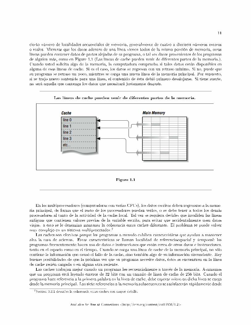
cierto número de localidades secuenciales de memoria, generalmente de cuatro a dieciseis números enteroso reales. Mientras que los datos adentro de una línea vienen todos de la misma porción de memoria, otraslíneas pueden contener datos de partes alejadas de su programa, o tal vez datos provenientes de los programasde alguien más, como en Figure 1.1 (Las líneas de cache pueden venir de diferentes partes de la memoria.).Cuando usted solicita algo de la memoria, la computadora comprueba si tales datos están disponibles enalguna de esas líneas de cache. Si es el caso, los datos se regresan con un retraso mínimo. Si no, puede quesu programa se retrase un poco, mientras se carga una nueva línea de la memoria principal. Por supuesto,si se trajo nuevo contenido para una línea, el contenido de ésta debió primero desalojarse. Si tiene suerte,no será aquella que contenga los datos que necesitará justamente después.
Las líneas de cache pueden venir de diferentes partes de la memoria.
Figure 1.1
En los multiprocesadores (computadoras con varias CPUs), los datos escritos deben regresarse a la memo-ria principal, de forma que el resto de los procesadores puedan verlos, o se debe tener a todos los demásprocesadores al tanto de la actividad de la cache local. Tal vez se requiera decirles que invaliden las líneasantiguas que contienen valores previos de la variable escrita, para evitar que accidentalmente usen datosviejos. a esto se le denomina mantener la coherencia entre caches diferentes. El problema se puede volvermuy complejo en un sistema multiprocesador.7
Las caches son efectivas porque los programas a menudo exhiben características que ayudan a manteneralta la tasa de aciertos. Estas características se llaman localidad de referenciaespacial y temporal; losprogramas frecuentemente hacen uso de datos e instrucciones que están cerca de otros datos e instrucciones,tanto en el espacio como en el tiempo. Cuando se carga una línea de cache de la memoria principal, no sólocontiene la información que causó el fallo de la cache, sino también algo de su información circundante. Haybuenas posibilidades de que la próxima vez que su programa necesite datos, éstos se encuentren en la líneade cache recién cargada o en alguna otra reciente.
Las caches trabajan mejor cuando un programa lee secuencialmente a través de la memoria. Asumamosque un programa está leyendo enteros de 32 bits con un tamaño de línea de cache de 256 bits. Cuando elprograma hace referencia a la primera palabra en la línea de cache, debe esperar mientras dicha línea se cargadesde la memoria principal. Las siete referencias a la memoria subsecuentes se satisfacerán rápidamente desde
7Section 3.2.1 describe la coherencia entre caches con mayor detalle.
Available for free at Connexions <http://cnx.org/content/col11356/1.2>
12 CHAPTER 1. ARQUITECTURAS DE CÓMPUTO MODERNAS
la cache. Esto se llama paso unitario porque la dirección de cada elemento de datos sucesivo se incrementaen uno, y se usan todos la datos cargados en la cache. El siguiente ciclo funciona con un paso unitario:
DO I=1,1000000
SUM = SUM + A(I)
END DO
Cuando un programa accede a una estructura de datos grande usando "pasos no unitarios", el rendimientosufre porque se cargan datos en cache que no se usan. Por ejemplo:
DO I=1,1000000, 8
SUM = SUM + A(I)
END DO
Este código carga la misma cantidad de datos y experimenta el mismo número de fallas en cache que el cicloprevio. Sin embargo, el programa necesita sólo una de las ocho palabras de 32 bits cargadas en la cache.Incluso aunque este programa realiza 1/8 de las sumas que el ciclo anterior, el tiempo que dilata en ejecutarsees aproximadamente el mismo que el otro, porque las operaciones de memoria dominan el rendimiento.
Aunque este ejemplo puede parecer un poco arti�cial, hay muchas situaciones en las cuales ocurrenfrecuentemente pasos no unitarios. Primero, cuando se carga en FORTRAN un arreglo bidimensional enmemoria, los elementos sucesivos en la primera columna se almacenan secuencialmente, seguidos por loselementos de la segunda columna. Si el arreglo se procesa colocando la iteración de los renglones en el ciclomás interno, produce un patrón de referencias de pasos unitarios como el siguiente:
REAL*4 A(200,200)
DO J = 1,200
DO I = 1,200
SUM = SUM + A(I,J)
END DO
END DO
Resulta interesante señalar que muy probablemente un programador en FORTRAN escribirá el ciclo (enorden alfabético) como sigue, produciendo un incremento no unitario de 800 bytes entre operaciones decarga sucesiva:
REAL*4 A(200,200)
DO I = 1,200
DO J = 1,200
SUM = SUM + A(I,J)
Available for free at Connexions <http://cnx.org/content/col11356/1.2>
13
END DO
END DO
Por esta razón, algunos compiladores pueden detectar este orden de ciclos subóptimo e invertirán el ordende los ciclos para lograr un mejor uso del sistema de memoria. Sin embargo, como veremos en Section 1.2.1,esta transformación de código puede producir resultados diferentes, y así usted deberá darle "permiso" alcompilador para intercambiar esos ciclos en este ejemplo particular (o, tras haber leído este libro, simplementehaberlo codi�cado apropiadamente desde el comienzo).
while ( ptr != NULL ) ptr = ptr->next;
El siguiente elemento que se recuerda se basa en el contenido del elemento actual. Este tipo de ciclo saltapor toda la memoria sin un patrón particular. Se le conoce como caza de apuntadores, y no existe una formaacertada de mejorar el rendimiento de este código.
Un tercer patrón que se encuentra a menudo en cierto tipo de códigos se conoce como acopio (o dispersión),y ocurre en ciclos como:
SUM = SUM + ARR ( IND(I) )
donde el arreglo IND contiene desplazamientos dentro del arreglo ARR. De nuevo, tal como sucedió en lalista ligada, el patrón exacto de referencias a memoria sólo se conoce a tiempo de ejecución, cuando tambiénse conocen los valores almacenados en el arreglo IND. Algunos sistemas de propósito especial tienen soportede hardware especializado para acelerar esta operación en particular.
1.1.5 Organización de la Cache8
El proceso de aparear las localidades de memoria con las líneas de cache se llama mapeo. Por supuesto,dado que la cache es menor que la memoria principal, tendrá usted que compartir las mismas líneas de cacheentre distintas localidades de memoria. En las caches, cada línea mantiene un registro de las direcciones dememoria (conocido como la etiqueta) a las que representa, y tal vez de cuándo se usaron por última vez. Laetiqueta se usa para seguir la pista a cuál área de memoria está almacenada en una línea particular de cache.
La forma en que las localidades de memoria (etiquetas) se mapean a líneas de cache puede tener unefecto bené�co en la forma en que se ejecuta su programa, porque si dos localidades de memoria utilizadasintensamente se mapean a la misma línea de cache, la tasa de fallos será mayor de lo que usted quisiera.Las caches pueden organizarse de varias maneras: mapeadas directamente, completamente asociativas yasociativas en conjunto.
1.1.5.1 Caches Mapeadas Directamente
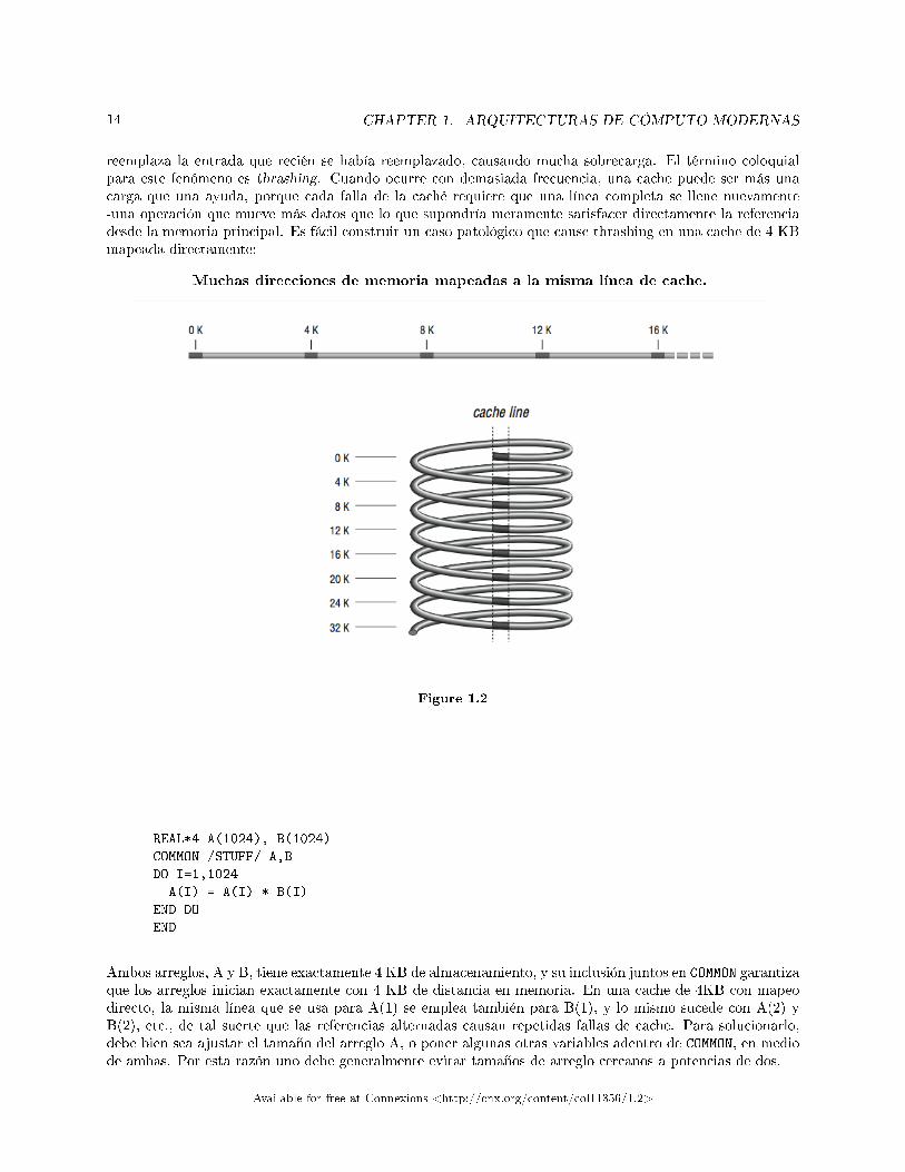
El mapeo directo, tal como se muestra en Figure 1.2 (Muchas direcciones de memoria mapeadas a la mismalínea de cache.), es el algoritmo más sencillo para decidir cómo mapear la memoria en la cache. Digamos,por ejemplo, que su computadora tiene 4 KB de cache. En un esquema de mapeo directo, la localidadde memoria 0 se mapea en la localidad 0 de cache, así como las localidades 4K, 8K, 12K, etc. En otraspalabras,la memoria se mapea en bloques del mismo tamaño que la cache. Otra forma de verlo es imaginarun resorte de metal con una línea de gis marcada a toda su longitud. Cada vuelta alrededor del resorte, seencuentra la línea de gis en el mismo lugar, módulo la longitud de circunferencia del resorte. Si éste es muylargo, la línea de gis cruza muchas vueltas de la bobina, análogo a como sucede con una memoria grandecon muchas localidades mapeándose a la misma línea de cache.
Los problemas devienen cuando a tiempo de ejecución se alternan referencias a memoria en un puntode la cache mapeada directamente, a la misma línea de cache. Cada referencia causa un fallo de caché y
8This content is available online at <http://cnx.org/content/m37227/1.2/>.
Available for free at Connexions <http://cnx.org/content/col11356/1.2>
14 CHAPTER 1. ARQUITECTURAS DE CÓMPUTO MODERNAS
reemplaza la entrada que recién se había reemplazado, causando mucha sobrecarga. El término coloquialpara este fenómeno es thrashing. Cuando ocurre con demasiada frecuencia, una cache puede ser más unacarga que una ayuda, porque cada falla de la caché requiere que una línea completa se llene nuevamente-una operación que mueve más datos que lo que supondría meramente satisfacer directamente la referenciadesde la memoria principal. Es fácil construir un caso patológico que cause thrashing en una cache de 4 KBmapeada directamente:
Muchas direcciones de memoria mapeadas a la misma línea de cache.
Figure 1.2
REAL*4 A(1024), B(1024)
COMMON /STUFF/ A,B
DO I=1,1024
A(I) = A(I) * B(I)
END DO
END
Ambos arreglos, A y B, tiene exactamente 4 KB de almacenamiento, y su inclusión juntos en COMMON garantizaque los arreglos inician exactamente con 4 KB de distancia en memoria. En una cache de 4KB con mapeodirecto, la misma línea que se usa para A(1) se emplea también para B(1), y lo mismo sucede con A(2) yB(2), etc., de tal suerte que las referencias alternadas causan repetidas fallas de cache. Para solucionarlo,debe bien sea ajustar el tamaño del arreglo A, o poner algunas otras variables adentro de COMMON, en mediode ambas. Por esta razón uno debe generalmente evitar tamaños de arreglo cercanos a potencias de dos.
Available for free at Connexions <http://cnx.org/content/col11356/1.2>
15
1.1.5.2 Cache Completamente Asociativa
En el extremo opuesto de una cache directamente mapeada se encuentra una cache completamente asociativa,donde cualquier localidad de memoria puede mapearse en cualquier línea de cache, independientemente dela dirección de memoria. Las caches completamente asociativas obtienen su nombre del tipo de memoriausada para construirlas -memoria asociativa- que es como la memoria regular, excepto por el hecho de quecada celda sabe algo acerca de los datos que contiene.
Cuando el procesador busca un dato, pregunta simultáeamente a todas las líneas de cache si alguna deellas lo tiene. La línea que contiene dicho dato alza su mano y dice "Lo tengo"; si ninguna contesta, ocurreuna falla de caché. Entonces viene la cuestión de cuál línea de cache debe reemplazarse con los nuevos datos.En vez de mapear las localidades de memoria a las líneas de cache mediante un algoritmo, como sucedeen el cache directamente mapeado, el sistema de memoria puede pedir a las líneas de cache completamenteasociativo que elijan entre ellas cuáles localidades de memoria representarán. Usualmente la línea que menosse ha usado recientemente es la que se sobreescribe con los nuevos datos. La presunción es que si los datosno han sido empleados durante un tiempo, es menos posible que se requieran en el futuro.
Las caches completamente asociativas presentan una utilización superior, cuando se comparan con cachesdirectamente mapeadas. Es difícil encontrar ejemplos de programas del mundo real que causen thrashingen un cache completamente asociativo. El precio de las caches completamente asociativas es muy alto, entérminos de tamaño, precio y velocidad. Las caches asociativas que realmente existen tienden a ser pequeñas.
1.1.5.3 Cache Asociativa en Conjunto
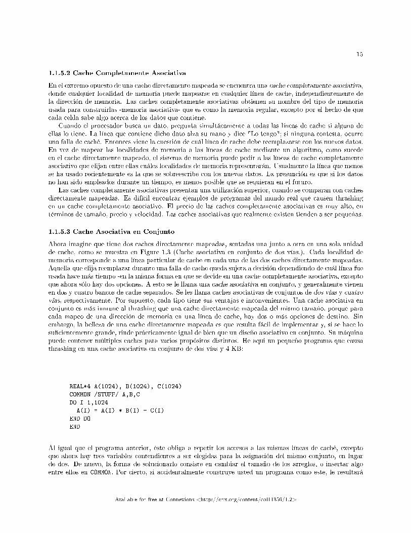
Ahora imagine que tiene dos caches directamente mapeadas, sentadas una junto a otra en una sola unidadde cache, como se muestra en Figure 1.3 (Cache asociativa en conjunto de dos vías.). Cada localidad dememoria corresponde a una línea particular de cache en cada una de las dos caches directamente mapeadas.Aquella que elija reemplazar durante una falla de cache queda sujeta a decisión dependiendo de cuál línea fueusada hace más tiempo -en la misma forma en que se decide en una cache completamente asociativa, exceptoque ahora sólo hay dos opciones. A esto se le llama una cache asociativa en conjunto, y generalmente vienenen dos y cuatro bancos de cache separados. Se les llama caches asociativas de conjuntos de dos vías y cuatrovías, respectivamente. Por supuesto, cada tipo tiene sus ventajas e inconvenientes. Una cache asociativa enconjunto es más inmune al thrashing que una cache directamente mapeada del mismo tamaño, porque paracada mapeo de una dirección de memoria en una línea de cache, hay dos o más opciones de destino. Sinembargo, la belleza de una cache directamente mapeada es que resulta fácil de implementar y, si se hace losu�cientemente grande, rinde prácticamente igual de bien que un diseño asociativo en conjunto. Su máquinapuede contener múltiples caches para varios propósitos distintos. He aqui un pequeño programa que causathrashing en una cache asociativa en conjunto de dos vías y 4 KB:
REAL*4 A(1024), B(1024), C(1024)
COMMON /STUFF/ A,B,C
DO I=1,1024
A(I) = A(I) * B(I) + C(I)
END DO
END
Al igual que el programa anterior, éste obliga a repetir los accesos a las mismas líneas de caché, exceptoque ahora hay tres variables contendientes a ser elegidas para la asignación del mismo conjunto, en lugarde dos. De nuevo, la forma de solucionarlo consiste en cambiar el tamaño de los arreglos, o insertar algoentre ellos en COMMON. Por cierto, si accidentalmente construye usted un programa como este, le resultará
Available for free at Connexions <http://cnx.org/content/col11356/1.2>

16 CHAPTER 1. ARQUITECTURAS DE CÓMPUTO MODERNAS
difícil detectarlo -más allá de sentir que el programa se ejecuta algo lento. Pocos proveedores proporcionanherramientas para medir las fallas de cache.
Cache asociativa en conjunto de dos vías.
Figure 1.3
1.1.5.4 Cache de Instrucciones
Hasta el momento hemos pasado por alto los dos tipos de información que se espera encontrar en una cacheubicada entre la memoria y la CPU: instrucciones y datos. Pero si piensa en ello, la demanda de datosse encuentra separada de la de instrucciones. En los procesadores superescalares, por ejemplo, es posibleejecutar una instrucción que causa una falla en la cache de datos junto con otras instrucciones que norequieren datos de la cache en absoluto, es decir, que operan sobre los registros. No parece justo que unafalla de cache en una referencia a datos en una instrucción deba evitarle recuperar otras instrucciones por quela cache está atada. Además, una cache depende localmente de la referencia entre bits de datos y otros bitsde datos o instrucciones y otras instrucciones, pero ¾qué clase de interdependencia existe entre instruccionesy datos? Parece imposible que las instrucciones extraigan datos perfectamente útiles de la cache, o viceversa,con completa independencia de la localidad de la referencia.
Muchos diseños desde la década de 1980 usan una sola cache tanto para instrucciones como para datos.Pero los diseños más nuevos están empleando lo que se conoce como la Arquitectura de Memoria Harvard,donde la demanda de datos se separa de la demanda de instrucciones.
La memoria todavía sigue siendo un único repositorio grande, pero estos procesadores tienen cachesseparadas de datos e instrucciones, posiblemente con diseños diferentes. Al proporcionar dos fuentes in-dependientes para datos e instrucciones, la tasa de información agregada proveniente de la memoria se
Available for free at Connexions <http://cnx.org/content/col11356/1.2>
17
incrementa, y la interferencia entre los dos tipos de referencias a memoria se minimiza. Además, las instruc-ciones generalmente tienen un nivel de localidad de referencia extremadamente alto, debido a la naturalezasecuencial de la mayoría de los programas. Como las caches de instrucciones no tienen que ser particular-mente grandes para ser efectivas, una arquitectura típica consiste en tener dos caches L1 separadas paradatos e instrucciones, y tener una cache L2 combinada. Por ejemplo, el PowerPC 604e de IBM/Motorolatiene caches L1 separadas de 32K de cuatro vías para instrucciones y datos, y una cache L2 combinada.
1.1.6 Memoria Virtual9
La memoria virtual desacopla las direcciones usadas por el programa (direcciones virtuales) de las direccionesdonde realmente está almacenado el dato en memoria (direcciones físicas). Su programa ve sus direccionescomenzando desde 0 y avanzando hasta algún número grande, pero las direcciones físicas a las que realmenteestán asignadas pueden ser muy diferentes. Esto proporciona cierto grado de �exibilidad, pues permite atodos los procesos creer que tienen el sistema de memoria completo para ellos. Otro rasgo de los sistemasde memoria virtual es que dividen la memoria de sus programas en páginas � fragmentos. Los tamaños depágina varían entre 512 bytes y 1 MB o más grande, dependiendo de la máquina. Las páginas no tienen porqué estar físicamente contiguas, aunque su programa las vea de esta forma. Al estar separados en páginas,los programas son más fáciles de acomodar en memoria, o mover porciones de los mismos hacia el disco.
1.1.6.1 Tablas de Páginas
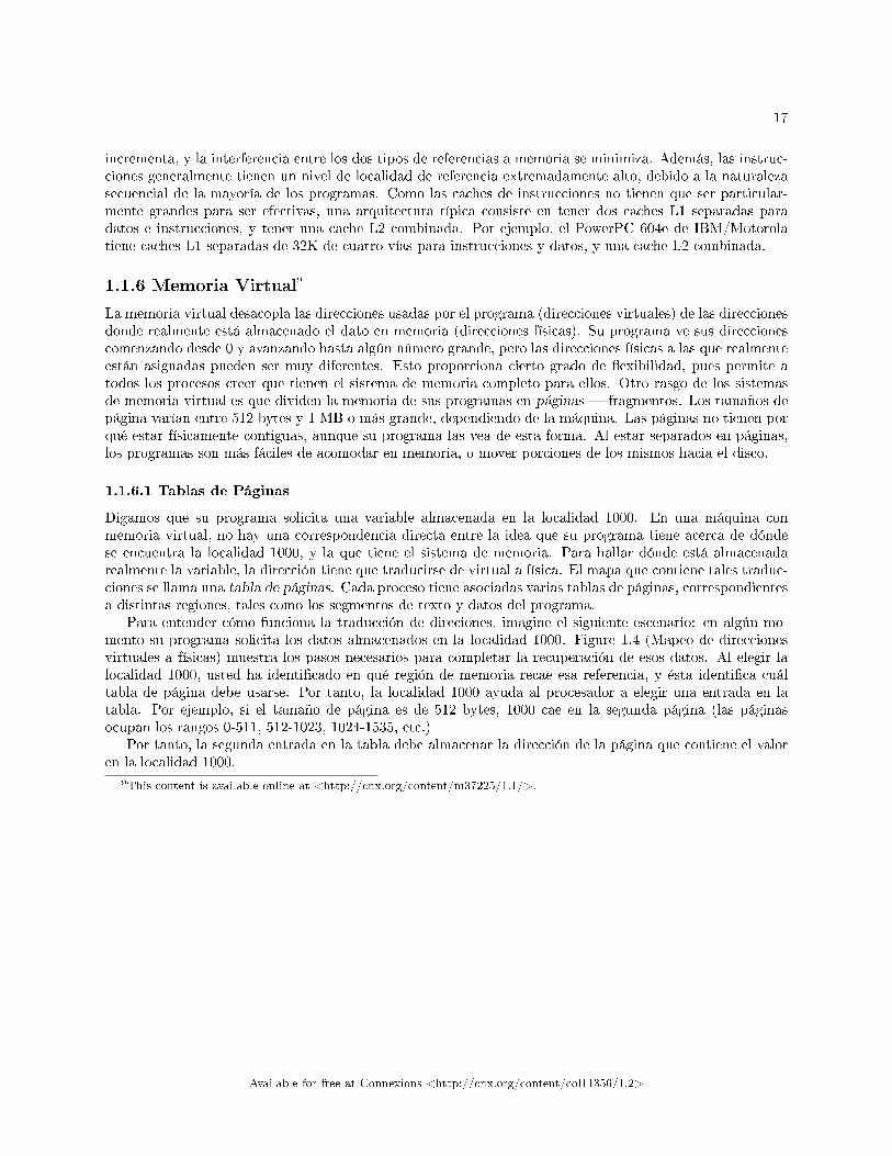
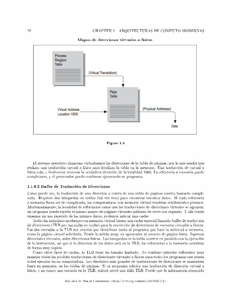
Digamos que su programa solicita una variable almacenada en la localidad 1000. En una máquina conmemoria virtual, no hay una correspondencia directa entre la idea que su programa tiene acerca de dóndese encuentra la localidad 1000, y la que tiene el sistema de memoria. Para hallar dónde está almacenadarealmente la variable, la dirección tiene que traducirse de virtual a física. El mapa que contiene tales traduc-ciones se llama una tabla de páginas. Cada proceso tiene asociadas varias tablas de páginas, correspondientesa distintas regiones, tales como los segmentos de texto y datos del programa.
Para entender cómo funciona la traducción de direciones, imagine el siguiente escenario: en algún mo-mento su programa solicita los datos almacenados en la localidad 1000. Figure 1.4 (Mapeo de direccionesvirtuales a físicas) muestra los pasos necesarios para completar la recuperación de esos datos. Al elegir lalocalidad 1000, usted ha identi�cado en qué región de memoria recae esa referencia, y ésta identi�ca cuáltabla de página debe usarse. Por tanto, la localidad 1000 ayuda al procesador a elegir una entrada en latabla. Por ejemplo, si el tamaño de página es de 512 bytes, 1000 cae en la segunda página (las páginasocupan los rangos 0-511, 512-1023, 1024-1535, etc.)
Por tanto, la segunda entrada en la tabla debe almacenar la dirección de la página que contiene el valoren la localidad 1000.
9This content is available online at <http://cnx.org/content/m37225/1.1/>.
Available for free at Connexions <http://cnx.org/content/col11356/1.2>
18 CHAPTER 1. ARQUITECTURAS DE CÓMPUTO MODERNAS
Mapeo de direcciones virtuales a físicas
Figure 1.4
El sistema operativo almacena virtualmente las direcciones de la tabla de páginas, por lo que tendrá querealizar una traducción virtual a física para localizar la tabla en la memoria. Una traducción de virtual afísica más, y �nalmente tenemos la verdadera dirección de la localidad 1000. La referencia a memoria puedecompletarse, y el procesador puede continuar ejecutando su programa.
1.1.6.2 Bu�er de Traducción de Direcciones
Como puede ver, la traducción de una dirección a través de una tabla de páginas resulta bastante compli-cada. Requiere dos búsquedas en tablas (tal vez tres) para encontrar nuestros datos. Si cada referenciaa memoria fuera así de complicada, las computadoras con memoria virtual tendrían rendimientos pésimos.Afortunadamente, la localidad de referencias causa que las traducciones de direcciones virtuales se agrupen;un programa puede repetir el mismo mapeo de páginas virtuales millones de veces por segundo. Y allí dondetenemos un uso repetido de los mismos datos, podemos aplicar una cache.
Todas las máquinas modernas con memoria virtual tienen una cache especial llamada bu�er de traducciónde direcciones (TLB por sus siglas en inglés) para la conversión de direcciones de memoria virtuales a físicas.Las dos entradas a la TLB son enteros que identi�can tanto al programa que hace la solicitud a memoria,como la página virtual solicitada. Desde la salida surge un apuntador al número de página física. Ingresandirecciones virtuales, salen direcciones físicas. Las búsquedas en la tabla ocurren en paralelo con la ejecuciónde la instrucción, así que si la dirección de los datos está en la TLB, las referencias a la memoria ocurriránde forma muy rápida.
Como otros tipos de caches, la TLB tiene un tamaño limitado. No contiene entradas su�cientes paramanejar todas las posibles traducciones de direcciones virtuales a físicas para todos los programas que puedausted ejecutar en su computadora. Los depósitos más grandes de traducciones de direcciones se mantienenfuera en memoria, en las tablas de páginas. Si su programa solicita una traducción de dirección virtual afísica, y no existe una entrada en la TLB, sufrirá usted una falla TLB. Puede que la información requerida
Available for free at Connexions <http://cnx.org/content/col11356/1.2>
19
deba generarse (es decir, crearse una nueva página), o puede que deba recuperarse de la tabla de páginas.La TLB es buena por la misma razón que lo son otros tipos de cahes: reducen el costo de hacer referencias
a memoria. Pero como las otras caches, existen casos patológicos en los cuales la TLB puede fallar en laentrega de un valor. El caso más sencillo de construir es uno donde cada referencia a memoria que haga suprograma cause una falla TLB:
REAL X(10000000)
COMMON X
DO I=0,9999
DO J=1,10000000,10000
SUM = SUM + X(J+I)
END DO
END DO
Asumamos que el tamaño de página de la TLB de su computadora es menor a 40 KB. Cada vez que serecorre el ciclo interno en el código de ejemplo anterior, el programa solicita datos que están alejadas 4bytes*10,000 = 40,000 bytes respecto a la última referencia. Esto es, cada referencia cae en una página dememoria diferente. Ello causa 1000 fallas TBL en el ciclo interior, repetido 1001 veces, para un total decuando menos un millón de fallas TLB. Para hacer todavía más grave el problema, está garantizado quecada referencia cause también una falla del cache de datos. Es claro que nada debe comenzar con un ciclocomo el de arriba. Pero suponiendo que el ciclo era del todo bueno para usted, la versión reestructurada delcódigo siguiente atraviesa la memoria como un cuchillo caliente la mantequilla:
REAL X(10000000)
COMMON X
DO I=1,10000000
SUM = SUM + X(I)
END DO
El ciclo revisado tiene saltos unitarios, y las fallas TLB ocurren sólo de modo muy ocasional. Usualmenteno es necesario a�nar explícitamente los programas para que hagan un buen uso de la TLB. Una vez que elprograma se modi�ca para ser "amigable con la cache", muy probablemente se haya a�nado también paraser amigable con la TLB.
Dado que hay bene�cios de rendimiento derivados de mantener muy pequeña la TLB, a menudo cadauna de sus entradas contiene un campo de longitud. Una sola entrada en la TLB puede tener cerca deun megabyte de longitud, y puede usarse para traducir direcciones almacenados en múltiples páginas dememoria virtual.
1.1.6.3 Fallos de Página
Cada elemento en la tabla de páginas también contiene otra información acerca de la página que representa,incluyendo banderas que indican si la traducción es válida, si la página asociada puede modi�carse, y algunainformación que describe cómo deben iniciarse las páginas nuevas. Aquellas referencias a páginas que noestán marcadas como válidas se denominan fallos de página.
Partiendo del peor escenario posible, digamos que su programa solicita una variable en una localidadde memoria particular. El procesador lo busca en la cache y encuentra que no está ahí (falla de cache), lo
Available for free at Connexions <http://cnx.org/content/col11356/1.2>
20 CHAPTER 1. ARQUITECTURAS DE CÓMPUTO MODERNAS
cual signi�ca que debe cargarse desde la memoria. Lo siguiente que hace es ir a la TLB para encontrar lalocalidad física del dato en memoria, y descubre que o hay una entrada en la TLB (una falla TLB). Entoncestrata de consultar la tabla de páginas (y rellenar nuevamente la TLB), pero encuentra que o bien no hayuna entrada para esta página en particular, o que dicha página se envió a disco (ambos casos son fallos depágina). Cada paso en la jerarquía de memoria ha complicado su solicitud. Debe crearse una nueva páginay posiblemente, dependiendo de las circunstancias, recargarla a partir del disco.
Pero independientemente de que tomen mucho tiempo, los fallos de página no son errores. Incluso bajocondiciones óptimas, cada programa sufre cierto número de fallos de página. Escribir una variable porprimera vez o llamar a una subrutina que no se había invocado previamente, causarán un fallo de página.Si no lo había pensado anteriormente puede parecerle sorpresivo. Existe la ilusión de que su programacompleto está presente en memoria desde el inicio, pero puede que ciertas porciones jamás se carguen. Nohay razón para hacerle espacio a una página a cuyos datos nunca se hace referencia, o cuyas instruccionesno se ejecutan. Sólo se crean o se traen del disco aquellas páginas que se necesitan para ejecutar el trabajo.10
El repositorio de páginas de memoria física está limitado, porque la memoria física también lo está, demodo que en una máquina en la que muchos programas cabildean por el espacio, ocurrirán una gran cantidadde fallos de página. Ello se debe a que las páginas de memoria física están reciclándose continuamente paraotros propósitos. Sin embargo, cuando tiene la máquina sólo para usted, y hay menos demanda de memoria,las páginas asignadas tienden a mantenerse por algún tiempo. En resumen, puede usted esperar menos fallosde página en una máquina tranquila. Un truco que debe recordar, si siempre termina usted trabajandopara un proveedor de computadoras: ejecute siempre benchmarks cortos dos veces. En algunos sistemas, elnúmero de fallos de página decaerá. Ello se debe a que la segunda ejecución encuentra páginas dejadas enmemoria por la primera, y usted no tiene que pagar el precio de los fallos de página nuevamente.11
El espacio de paginación (espacio de intercambio) en el disco es la última y más lenta de las piezas dela jerarquía de memoria en la mayoría de las máquinas. En el peor escenario vimos cómo puede enviarseuna referencia a memoria hacia un medio más lento y con un rendimiento inferior, antes de que �nalmentese satisfaga la solicitud. Si se regresa sobre sus pasos, podrá ver que el espacio de paginación en disco tienela misma relación con la memoria principal, que ésta respecto a la cache. También se aplican las mismasclases de optimización, y la localidad de las referencias es importante. Puede ejecutar programas mayoresque la memoria principal de su máquina, pero a veces a costa de una gran caída del rendimiento. Cuandorevisemos las optimizaciones de memoria en here12, nos concentraremos en mantener en actividad las partesmás rápidas del sistema de memoria, y evitar las más lentas.
1.1.7 Mejorando el Rendimiento de la Memoria13
Dada la importancia, en el área del cómputo de alto rendimiento, del desempeño del subsistema de memoriade una computadora, se han usado muchas técnicas para tratar de mejorarlo. Sus dos atributos más impor-tantes son el ancho de banda y la latencia. Ciertos diseños de sistemas de memoria mejoran uno a expensasdel otro, mientras que otros impactan positivamente tanto en el ancho de banda como en la latencia. Elancho de banda generalmente se enfoca en la mejor tasa de transferencia del sistema de memoria en estadoestacionario, lo que usualmente se mide durante la ejecución de un ciclo largo de avance unitario, que lee olee y escribe la memoria. 14 La latencia es una medida del rendimiento de un sistema de memoria, en el peorcaso conforme mueve una pequeña cantidad de datos (como por ejemplo una palabra de 32 o 64 bits) entreel procesador y la memoria. Ambos son importantes porque son parte sustancial de muchas aplicaciones dealto rendimiento.
Como los sistemas de memoria se dividen en componentes, hay valores de ancho de banda y latencia de
10El término adecuado para referirse a esto es demanda de páginas.11El dispositivo de disco identi�ca las páginas de texto y los números de bloque de los que procede.12"Loop Optimizations - Introduction" <http://cnx.org/content/m33728/latest/>13This content is available online at <http://cnx.org/content/m37224/1.1/>.14Véase la sección FLUJO del documento=""/>Capítulo 15 para una revisión de las medidas del ancho de banda de la
memoria.
Available for free at Connexions <http://cnx.org/content/col11356/1.2>
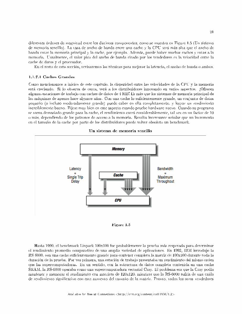
21
diferentes órdenes de magnitud entre los distintos componentes, como se muestra en Figure 1.5 (Un sistemade memoria sencillo). La tasa de ancho de banda entre una cache y la CPU será más alta que el ancho debanda entre la memoria principal y la cache, por ejemplo. Además, puede haber muchas caches y rutas a lamemoria. Usualmente, el valor pico del ancho de banda citado por los vendedores es la velocidad entre lacache de datos y el procesador.
En el resto de esta sección, revisaremos las técnicas para mejorar la latencia, el ancho de banda o ambos.
1.1.7.1 Caches Grandes
Como mencionamos a inicios de este capítulo, la disparidad entre las velocidades de la CPU y la memoriaestá creciendo. Si lo observa de cerca, verá a los distribuidores innovando en varios aspectos. ½Ofrecenalgunas estaciones de trabajo con caches de datos de 4 MB! Es más que los sistemas de memoria principal delas máquinas de apenas hace algunos años. Con una cache lo su�cientemente grande, un conjunto de datospequeño (o incluso moderadamente grande) puede caber en ella completamente, y lograr un rendimientoincreíblemente bueno. Fíjese muy bien en este aspecto cuando pruebe hardware nuevo. Cuando su programase torna demasiado grande para la cache, el rendimiento caerá considerablemente, tal vez en un factor de 10o más, dependiendo de los patrones de acceso a la memoria. Resulta interesante señalar que un incrementoen el tamaño de la cache por parte de los distribuidores puede volver obsoleto un benchmark.
Un sistema de memoria sencillo
Figure 1.5
Hasta 1999, el benchmark Linpack 100x100 fue probablemente la prueba más respetada para determinarel rendimiento promedio comparativo de una amplia variedad de aplicaciones. En 1992, IBM introdujo laRS-6000, con una cache su�cientemente grande para contener completa la matriz de 100x100 durante toda laduración de la prueba. Por vez primera, una estación de trabajo presentaba un rendimiento del mismo ordenque las supercomputadoras. En un sentido, con la estructura de datos completa contenida en una cacheSRAM, la RS-6000 operaba como una supercomputadora vectorial Cray. El problema era que la Cray podíamantener y memorar el rendimiento con matrices de 120x120, mientras que la RS-6000 sufría de una caídade rendimiento signi�cativo con este aumento del tamaño de la matriz. Pronto, todos los otros vendedores
Available for free at Connexions <http://cnx.org/content/col11356/1.2>
22 CHAPTER 1. ARQUITECTURAS DE CÓMPUTO MODERNAS
de estaciones de trabajo introdujeron caches de tamaño similar, y la prueba Linpack 100x100 dejó de ser útilcomo un indicador del rendimiento promedio de una aplicación.
1.1.7.2 Sistemas de Memoria más Anchos
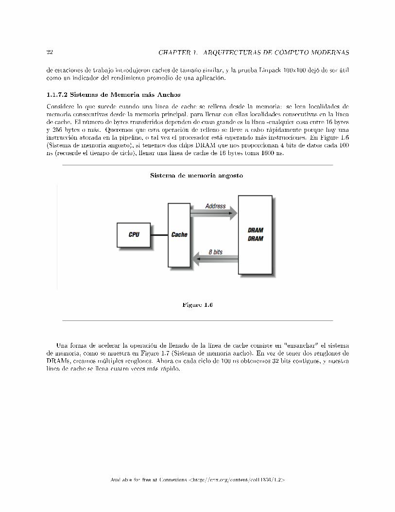
Considere lo que sucede cuando una línea de cache se rellena desde la memoria: se leen localidades dememoria consecutivas desde la memoria principal, para llenar con ellas localidades consecutivas en la líneade cache. El número de bytes transferidos dependen de cuan grande es la línea -cualquier cosa entre 16 bytesy 256 bytes o más. Queremos que esta operación de relleno se lleve a cabo rápidamente porque hay unainstrucción atorada en la pipeline, o tal vez el procesador está esperando más instrucciones. En Figure 1.6(Sistema de memoria angosto), si tenemos dos chips DRAM que nos proporcionan 4 bits de datos cada 100ns (recuerde el tiempo de ciclo), llenar una línea de cache de 16 bytes toma 1600 ns.
Sistema de memoria angosto
Figure 1.6
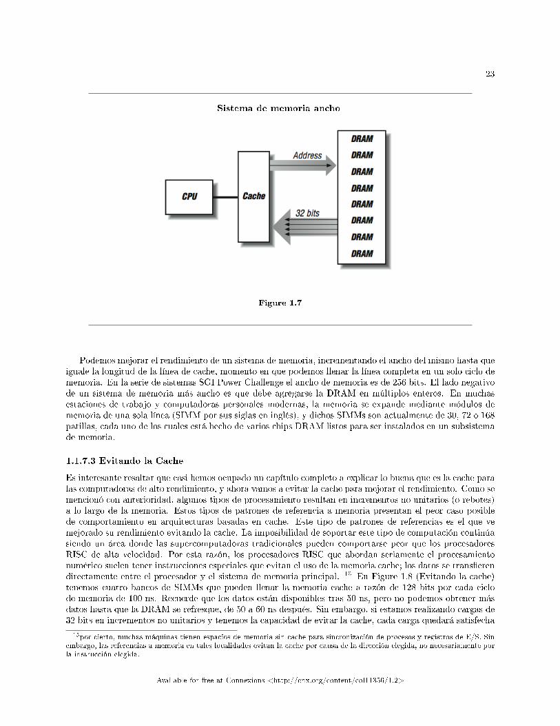
Una forma de acelerar la operación de llenado de la línea de cache consiste en "ensanchar" el sistemade memoria, como se muestra en Figure 1.7 (Sistema de memoria ancho). En vez de tener dos renglones deDRAMs, creamos múltiples renglones. Ahora en cada ciclo de 100 ns obtenemos 32 bits contiguos, y nuestralínea de cache se llena cuatro veces más rápido.
Available for free at Connexions <http://cnx.org/content/col11356/1.2>
23
Sistema de memoria ancho
Figure 1.7
Podemos mejorar el rendimiento de un sistema de memoria, incrementando el ancho del mismo hasta queiguale la longitud de la línea de cache, momento en que podemos llenar la línea completa en un solo ciclo dememoria. En la serie de sistemas SGI Power Challenge el ancho de memoria es de 256 bits. El lado negativode un sistema de memoria más ancho es que debe agregarse la DRAM en múltiplos enteros. En muchasestaciones de trabajo y computadoras personales modernas, la memoria se expande mediante módulos dememoria de una sola línea (SIMM por sus siglas en inglés), y dichos SIMMs son actualmente de 30, 72 o 168patillas, cada uno de los cuales está hecho de varios chips DRAM listos para ser instalados en un subsistemade memoria.
1.1.7.3 Evitando la Cache
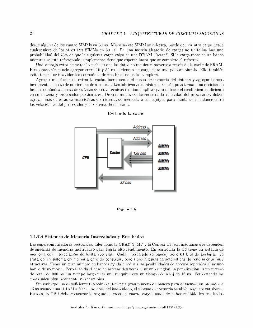
Es interesante resaltar que casi hemos ocupado un capítulo completo a explicar lo buena que es la cache paralas computadoras de alto rendimiento, y ahora vamos a evitar la cache para mejorar el rendimiento. Como semencionó con anterioridad, algunos tipos de procesamiento resultan en incrementos no unitarios (o rebotes)a lo largo de la memoria. Estos tipos de patrones de referencia a memoria presentan el peor caso posiblede comportamiento en arquitecturas basadas en cache. Este tipo de patrones de referencias es el que vemejorado su rendimiento evitando la cache. La imposibilidad de soportar este tipo de computación continúasiendo un área donde las supercomputadoras tradicionales pueden comportarse peor que los procesadoresRISC de alta velocidad. Por esta razón, los procesadores RISC que abordan seriamente el procesamientonumérico suelen tener instrucciones especiales que evitan el uso de la memoria cache; los datos se trans�erendirectamente entre el procesador y el sistema de memoria principal. 15 En Figure 1.8 (Evitando la cache)tenemos cuatro bancos de SIMMs que pueden llenar la memoria cache a razón de 128 bits por cada ciclode memoria de 100 ns. Recuerde que los datos están disponibles tras 50 ns, pero no podemos obtener másdatos hasta que la DRAM se refresque, de 50 a 60 ns después. Sin embargo, si estamos realizando cargas de32 bits en incrementos no unitarios y tenemos la capacidad de evitar la cache, cada carga quedará satisfecha
15por cierto, muchas máquinas tienen espacios de memoria sin cache para sincronización de procesos y registros de E/S. Sinembargo, las referencias a memoria en tales localidades evitan la cache por causa de la dirección elegida, no necesariamente porla instrucción elegida.
Available for free at Connexions <http://cnx.org/content/col11356/1.2>
24 CHAPTER 1. ARQUITECTURAS DE CÓMPUTO MODERNAS
desde alguno de los cuatro SIMMs en 50 ns. Mientras ese SIMM se refresca, puede ocurrir otra carga desdecualesquiera de los otros tres SIMMs en 50 ns. En una mezcla aleatoria de cargas no unitarias hay unaprobabilidad del 75% de que la siguiente carga caiga en una DRAM "fresca". Si la carga recae en un bancomientras se está refrescando, simplemente tiene que esperar hasta que se complete el refresco.
Una ventaja extra de evitar la cache es que los datos no requieren moverse a través de la cache de SRAM.Esta operación puede agregar entre 10 y 50 ns al tiempo de carga para una palabra simple. Ello tambiénevita tener que invalidar los contenidos de una línea de cache completa.
Agregar una forma de evitar la cache, incrementar el ancho de memoria del sistema y agregar bancosincrementa el costo de un sistema de memoria. Los fabricantes de sistemas de cómputo toman una decisión deíndole económica acerca de cuántas de estas técnicas requieren aplicar para obtener el rendimiento su�cienteen su sistema y procesador particulares. De este modo, conforme crece la velocidad del procesador, debenagregar más de estas características del sistema de memoria a sus equipos para mantener el balance entrelas velocidades del procesador y el sistema de memoria.
Evitando la cache
Figure 1.8
1.1.7.4 Sistemas de Memoria Intercalados y Entubados
Las supercomputadoras vectoriales, tales como la CRAY Y/MP y la Convex C3, son máquinas que dependende sistemas de memoria multibanco para lograr alto rendimiento. En particular la C3 tiene un sistema dememoria con intercalación de hasta 256 vías. Cada intercalado (o banco) tiene 64 bits de anchura. Setrata de un sistema de memoria caro de construir, pero tiene algunas características de rendimiento muyatractivas. Tener un gran número de bancos ayuda a reducir las posibilidades de accesos repetidos al mismobanco de memoria. Pero si se da el caso de acertar dos veces al mismo renglón, la penalización es un retrasode cerca de 300 ns -un tiempo largo para una máquina con un tiempo de reloj de 16 ns. Pero cuando lascosas salen bien, realmente van muy bien.
Sin embargo, no es su�ciente tan sólo con tener un gran número de bancos para alimentar un prosador a16 ns usando una DRAM a 50 ns. Además del intercalado, el sistema de memoria también requiere entubarse.Esto es, la CPU debe comenzar la segunda, tercera y cuarta cargas antes de haber recibido los resultados
Available for free at Connexions <http://cnx.org/content/col11356/1.2>
25
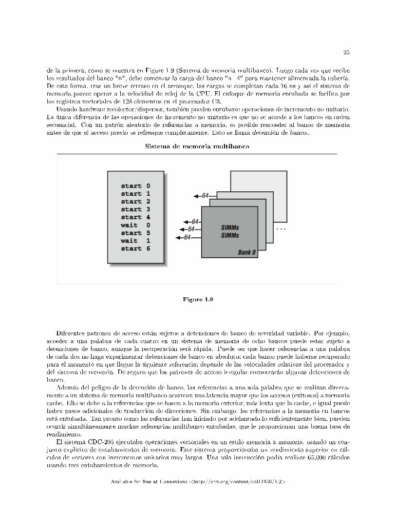
de la primera, como se muestra en Figure 1.9 (Sistema de memoria multibanco). Luego cada vez que recibelos resultados del banco "n", debe comenzar la carga del banco "n+4" para mantener alimentada la tubería.De esta forma, tras un breve retraso en el arranque, las cargas se completan cada 16 ns y así el sistema dememoria parece operar a la velocidad de reloj de la CPU. El enfoque de memoria entubada se facilita porlos registros vectoriales de 128 elementos en el procesador C3.
Usando hardware recolector/dispersor, también pueden entubarse operaciones de incremento no unitario.La única diferencia de las operaciones de incremento no unitario es que no se accede a los bancos en ordensecuencial. Con un patrón aleatorio de referencias a memoria, es posible reacceder al banco de memoriaantes de que el acceso previo se refresque completamente. Esto se llama detención de banco..
Sistema de memoria multibanco
Figure 1.9
Diferentes patrones de acceso están sujetos a detenciones de banco de severidad variable. Por ejemplo,acceder a una palabra de cada cuatro en un sistema de memoria de ocho bancos puede estar sujeto adetenciones de banco, aunque la recuperación será rápida. Puede ser que hacer referencias a una palabrade cada dos no haga experimentar detenciones de banco en absoluto; cada banco puede haberse recuperadopara el momento en que llegue la siguiente referencia; depende de las velocidades relativas del procesador ydel sistema de memoria. De seguro que los patrones de acceso irregular encontrarán algunas detenciones debanco.
Además del peligro de la detención de banco, las referencias a una sola palabra que se realizan directa-mente a un sistema de memoria multibanco acarrean una latencia mayor que los accesos (exitosos) a memoriacache. Ello se debe a la referencias que se hacen a la memoria exterior, más lenta que la cache, e igual puedehaber pasos adicionales de traducción de direcciones. Sin embargo, las referencias a la memoria en bancosestá entubada. Tan pronto como las referencias han iniciado por adelantado lo su�cientemente bien, puedenocurrir simultáneamente muchas referencias multibanco entubadas, que le proporcionan una buena tasa derendimiento.
El sistema CDC-205 ejecutaba operaciones vectoriales en un estilo memoria a memoria, usando un con-junto explícito de entubamientos de memoria. Este sistema proporcionaba un rendimiento superior en cál-culos de vectores con incrementos unitarios muy largos. Una sola instrucción podía realizar 65,000 cálculosusando tres entubamientos de memoria.
Available for free at Connexions <http://cnx.org/content/col11356/1.2>
26 CHAPTER 1. ARQUITECTURAS DE CÓMPUTO MODERNAS
1.1.7.5 Caches Administradas por Software
He aquí una idea interesante: si un procesador vectorial puede plani�car el arranque de un entubamientode memoria con su�ciente antelación, ¾por qué no puede un procesador RISC comenzar un llenado de cacheantes de que requiera los datos en esa misma situación? De esta forma, está aprestando la cache para ocultarla latencia del llenado de la misma. Si puede realizarse con su�ciente antelación, dará la impresión que todaslas referencias a memoria operan a la velocidad de la cache.
Este concepto se llama precarga (prefetch) y está soportado mediante el uso de una instrucción especialde precarga disponible en muchos procesadores RISC. Tal instrucción opera exactamente igual que unaoperación de carga común, excepto que el procesador no espera que la cache se llene antes de completar lainstrucción. La idea es precargar lo su�ciente como para tener los datos listos en cache al momento en quese realiza el cálculo. El siguiente ejemplo ilustra cómo se usa:
DO I=1,1000000,8
PREFETCH(ARR(I+8))
DO J=0,7
SUM=SUM+ARR(I+J)
END DO
END DO
Esto no es realmente FORTRAN. La precarga usualmente se realiza en el código ensamblador generado porel compilador cuando detecta que usted está saltando a lo largo del arreglo usando un salto de tamaño �jo.El compilador típicamente estima cuán adelante debe precargar. En el ejemplo anterior, si el llenado de lacache fuera particularmente lento, el valor 8 en I+8 puede cambiarse a 16 o 32 mientras los demás valoresse cambien en consonancia.
En un procesador que sólo puede ejecutar una instrucción por ciclo, podría no valer la pena precargaruna instrucción; el intercambio tomaría tiempo valioso en el �ujo de instrucciones de entrada, con bene�ciosdudosos. En un procesador superescalar, sin embargo, puede mezclarse un aviso de cache con el resto del�ujo de instrucciones, y emitirlo entre otras instrucciones reales. Si ello salva a su programa de sufrir fallosde cache extra, valdrá la pena.
1.1.7.6 Efectos Post-RISC sobre las Referencias a Memoria
En un procesador RISC, las operaciones de memoria típicamente acceden a ésta durante la fase de ejecucióndel entubamiento. En el procesador post-RISC, las cosas no son diferentes que en un procesador RISC,excepto que en un momento dado muchas cargas pueden estar a medio terminar. En algunos procesadoresactuales pueden estar activas hasta 28 operaciones de memoria, con 10 en espera de salir de la memoria.Esta es una forma excelente de compensar la latencia de una memoria lenta comparada con la velocidad dela CPU. Considere el siguiente ciclo:
LOADI R6,10000 El número de iteraciones
LOADI R5,0 La variable índice
CICLO: LOAD R1,R2(R5) Carga un valor de la memoria
INCR R1 Suma 1 a R1
STORE R1,R3(R5) Almacena el valor incrementado de vuelta en la memoria
INCR R5 Suma 1 a R5
Available for free at Connexions <http://cnx.org/content/col11356/1.2>
27
COMPARE R5,R6 Comprueba la terminación del ciclo
BLT CICLO si R5 = R6, salta a CICLO
Asumamos en este ejemplo que toma 50 ciclos acceder a la memoria. Cuando la búsqueda/decodi�caciónpone la primera carga en el bu�er de reordenamiento de instrucciones (IRB), la carga comienza en el siguienteciclo y luego se suspende en la fase de ejecución. Sin embargo, el resto de las instrucciones están en el IRB. Lainstrucción INCR R1 debe esperar a la carga, y la instrucción STORE también debe esperar. Sin embargo,al usar un registro renombrado, las instrucciones INCR R5, COMPARE y BLT pueden todas ejecutarse, yla búsqueda/decodi�cación avanza a la parte superior del ciclo y envía otra carga al IRB para la siguientelocalidad de memoria que tiene que esperar. Esta secuencia continúa hasta que se hayan cargado unas 10iteraciones del ciclo en la TLB. Es entonces cuando se entrega la primera carga desde la memoria, y comienzana ejecutarse las instrucciones INCR 1 y STORE de la primera iteración. Por supuesto el almacenamientotoma algo de tiempo, pero alrededor de ese momento termina la segunda carga, de modo que hay más trabajopor hacer, y así sucesivamente...
Como muchos otros aspectos de la computación, la arquitectura post-RISC, con su ejecución especulativafuera de orden, optimiza las referencias a memoria. El procesador post-RISC desenrolla los ciclos dinámi-camente, a tiempo de ejecución, para compensar los retrasos del subsistema de memoria. Asumiendo unsistema de memoria multibanco con entubamiento, que puede tener iniciadas múltiples operaciones de memo-ria antes de que alguna se complete (la HP PA-8000 tiene simultáneamente 10 operaciones de memoria fueradel chip al vuelo), el procesador continúa despachando operaciones a memoria hasta que tales operacionescomiencen a completarse.
A diferencia de un procesador vectorial o una instrucción de precarga, el procesador post-RISC nonecesita anticipar el patrón preciso de referencias a memoria, de forma que puede controlar cuidadosamenteel subsistema de memoria. Como resultado, el procesador post-RISC puede lograr su rendimiento máximoen un rango mucho más amplio de secuencias de código que los procesadores vectoriales y los procesadoresRISC de ejecución en orden con capacidad de precarga.
La tolerancia implícita a la latencia de memoria hace a los procesadores post-RISC ideales para usarseen los procesadores escalables de memoria compartida del futuro, donde la jerarquía de memoria se harátodavía más compleja que en los procesadores actuales con tres niveles de cache y una memoria principal.
Desafortunadamente, el único segmento de código que no se bene�cia signi�cativamente de la arquitecturadel post-RISC es el recorrido de listas ligadas. Ello se debe a que nunca se conoce la siguiente direcciónhasta que se completa la carga previa, de forma que todas las cargas están fundamentalmente seriadas.
1.1.7.7 Tendencias en Tecnologías de RAM Dinámica
Muchas de las técnicas en esta sección se han enfocado en cómo lidiar con las imperfecciones de los chipsde RAM dinámica (aunque cuando su tasa de velocidad de reloj alcanza los 300-600 MHz o 3-2 ns, inclusola SRAM comienza a parecer muy lenta). Es claro que la demanda por cada vez más RAM continuaráincrementándose, y que digabits y más DRAM cupirán en un solo chip. Por ello, se está trabajando muchopara crear nuevas súper DRAMs más rápidas y mejor preparadas para los procesadores extremadamenterápidos del presente y del futuro. Algunas de las tecnologías son relativamente sencillas, mientras que otrasrequieren importantes rediseños en la forma en que procesadores y memorias se fabrican.
Entre las mejoras de la DRAM se incluyen:
• DRAM de modo de página rápida• RAM de salida de datos extendida (EDO RAM)• DRAM síncrona (SDRAM)• RAMBUS• DRAM con cache (CDRAM)
La DRAM de modo de página rápida ahorra tiempo al permitir un modo en el cuál no tiene que re-programarse la dirección completa en el chip para cada operación de memoria. En vez de ello, se asume que
Available for free at Connexions <http://cnx.org/content/col11356/1.2>
28 CHAPTER 1. ARQUITECTURAS DE CÓMPUTO MODERNAS
se accederá a la memoria secuencialmente (como en el llenado de una línea de cache), y sólo los bits de ordenbajo de la dirección se modi�can en las lecturas y escrituras sucesivas.
La EDO RAM es una modi�cación al mecanismo de bu�er de salida en la RAM de modo de página, quele permite operar cerca del doble de rápido en operaciones que no sean de refresco.
La DRAM síncrona se sincroniza usando un reloj externo que permite a la cache y a la DRAM coordinarsus operaciones. Así, la SRAM puede entubar el recuperación de múltiples bits de memoria para mejorar elrendimiento global.
RAMBUS es una tecnología propietaria, capaz de transferir datos a 500 MB/seg. Usa una cantidadsigni�cativa de lógica adentro del chip, y opera a niveles de energía mayores que la DRAM típica.
La DRAM con cache combina una cache SRAM en el mismo chip que la DRAM. Con ello ambas quedanfuertemente acopladas, proporcionando rendimientos similares a dispositivos SRAM con todas las limita-ciones de cualquier arquitectura de cache. Una ventaja del enfoque CDRAM es que incrementa la cantidadde cache y disminuye la cantidad de DRAM. También cuando se trabaja con sistemas de memoria con ungran número de intercalaciones, cada una tiene su propia SRAM para reducir la latencia, asumiendo que losdatos solicitados estuvieran en la SRAM.
Un enfoque todavía más avanzado consiste en integrar procesador, SRAM y DRAM en un un único chipcon un reloj a, digamos, 5 GHz, conteniendo 128 MB de datos. Comprensiblemente, hay una amplia variedadde problemas técnicos que resolver antes de que este tipo de componente esté ampliamente disponible porUS$200 -pero esa no es toda la cuestión. Los procesos de manufactura de la DRAM y los procesadores yaestán comenzando a converger en algunas formas (RAMBUS). El mayor problema de rendimiento cuandotengamos esta clase de sistema será, "¾qué hacer si usted necesita 160 MB?"
1.1.8 Notas de Cierre16
Se dice que la computadora del futuro será un buen sistema de memoria, que simplemente traiga conectadauna CPU. Para que los sistemas de microprocesadores de alto rendimiento tomen el relevo como los motoresde cómputo de alto rendimiento, el problema de un sistema de memoria basado en cache que usa DRAM parasu memoria principal debe solucionarse. Hay muchos esfuerzos en desarrollo de arquitecturas y tecnologías,para transformar las memorias de las estaciones de trabajo y computadoras personales, y darles capacidadescomo las memorias de las supercomputadoras.
Conforme la velocidad de la CPU se incremente más rápido que la de la memoria, usted necesitará delas técnicas de este libro. Además, conforme se mueva hacia los procesadores múltiples, los problemas nomejorarán; usualmente se volverán peores. Con muchos procesadores constantemente hambrientos por másdatos, un subsistema de memoria puede volverse extremadamente tenso.
Con sólo un poco de habilidad, a menudo podemos reestructurar los accesos a memoria, de forma tal queaprovechen las fortalezas de su sistema de memoria, en vez de sus debilidades.
1.1.9 Ejercicios17
Exercise 1.1.9.1El siguiente segmento de código recorre una cadena de apuntadores:
while ((p = (char *) *p) != NULL);
¾Cómo interactuará este código con la cache si todas las referencias caen en una pequeña porciónde memoria? ¾Cómo interactuará con la cache si las referencias se prolongan a través de variosmegabytes?
Exercise 1.1.9.2¾Cómo se comportará el código en Exercise 1.1.9.1 en un sistema de memoria multibanco que notenga cache?
16This content is available online at <http://cnx.org/content/m37226/1.1/>.17This content is available online at <http://cnx.org/content/m37221/1.1/>.
Available for free at Connexions <http://cnx.org/content/col11356/1.2>

29
Exercise 1.1.9.3Hace mucho tiempo, la gente escribía regularmente código automodi�cable -programas que escribenen la memoria de instrucciones y cambian su propio comportamiento. ¾Cuáles son las implicacionesde código automodi�cable en una máquina con una arquitectura de memoria Harvard?
Exercise 1.1.9.4Asuma una arquitectura de memoria con una velocidad de cache L1 de 10 ns, una velocidad L2de 30 ns, y una velocidad de memoria de 200 ns. Compare el rendimiento promedio del sistema dememoria con: 1) L1 80%, L2 10% y memoria 10%; y 2) L1 85% y memoria 15%.
Exercise 1.1.9.5En un sistema de cómputo, ejecute ciclos que procesen arreglos de longitudes variables de 16 a 16millones:
ARRAY(I) = ARRAY(I) + 3
¾Cómo cambia el número de sumas por segundo conforme la longitud del arreglo cambia? Experi-mente con REAL*4, REAL*8, INTEGER*4, e INTEGER*8.
¾Qué tiene un impacto más signi�cativo en el rendimiento, elementos de arreglo más grandes onúmeros enteros versus números de punto �otante? Realice pruebas en una variedad de computa-doras diferentes.
Exercise 1.1.9.6Elabore un arreglo bidimensional de 1024x1024. Recorra el array, con los renglones como ciclointerno y después con las columnas como ciclo interno. Realice alguna operación simple en cadaelemento. ¾Se comportan distinto los ciclos? ¾Por qué? Experimente con diferentes dimensionesde arreglos y vea el impacto en el rendimiento.
Exercise 1.1.9.7Escriba un programa que ejecute repetidamente ciclos temporizados de diferentes tamaños, paradeterminar el tamaño de cache de su sistema.
1.2 Números de Punto Flotante
1.2.1 Introduction18
Often when we want to make a point that nothing is sacred, we say, �one plus one does not equal two.� Thisis designed to shock us and attack our fundamental assumptions about the nature of the universe. Well, inthis chapter on �oating- point numbers, we will learn that �0.1+0.1 does not always equal 0.2� when we use�oating-point numbers for computations.
In this chapter we explore the limitations of �oating-point numbers and how you as a programmer canwrite code to minimize the e�ect of these limitations. This chapter is just a brief introduction to a signi�cant�eld of mathematics called numerical analysis.
1.2.2 Reality19
The real world is full of real numbers. Quantities such as distances, velocities, masses, angles, and otherquantities are all real numbers.20 A wonderful property of real numbers is that they have unlimited accuracy.For example, when considering the ratio of the circumference of a circle to its diameter, we arrive at a valueof 3.141592.... The decimal value for pi does not terminate. Because real numbers have unlimited accuracy,
18This content is available online at <http://cnx.org/content/m32739/1.3/>.19This content is available online at <http://cnx.org/content/m32741/1.3/>.20In high performance computing we often simulate the real world, so it is somewhat ironic that we use simulated real numbers
(�oating-point) in those simulations of the real world.
Available for free at Connexions <http://cnx.org/content/col11356/1.2>
30 CHAPTER 1. ARQUITECTURAS DE CÓMPUTO MODERNAS
even though we can't write it down, pi is still a real number. Some real numbers are rational numbers becausethey can be represented as the ratio of two integers, such as 1/3. Not all real numbers are rational numbers.Not surprisingly, those real numbers that aren't rational numbers are called irrational. You probably wouldnot want to start an argument with an irrational number unless you have a lot of free time on your hands.
Unfortunately, on a piece of paper, or in a computer, we don't have enough space to keep writing thedigits of pi. So what do we do? We decide that we only need so much accuracy and round real numbers toa certain number of digits. For example, if we decide on four digits of accuracy, our approximation of pi is3.142. Some state legislature attempted to pass a law that pi was to be three. While this is often cited asevidence for the IQ of governmental entities, perhaps the legislature was just suggesting that we only needone digit of accuracy for pi. Perhaps they foresaw the need to save precious memory space on computerswhen representing real numbers.
1.2.3 Representation21
Given that we cannot perfectly represent real numbers on digital computers, we must come up with acompromise that allows us to approximate real numbers.22 There are a number of di�erent ways that havebeen used to represent real numbers. The challenge in selecting a representation is the trade-o� betweenspace and accuracy and the tradeo� between speed and accuracy. In the �eld of high performance computingwe generally expect our processors to produce a �oating- point result every 600-MHz clock cycle. It is prettyclear that in most applications we aren't willing to drop this by a factor of 100 just for a little more accuracy.Before we discuss the format used by most high performance computers, we discuss some alternative (albeitslower) techniques for representing real numbers.
1.2.3.1 Binary Coded Decimal
In the earliest computers, one technique was to use binary coded decimal (BCD). In BCD, each base-10 digitwas stored in four bits. Numbers could be arbitrarily long with as much precision as there was memory:
123.45
0001 0010 0011 0100 0101
This format allows the programmer to choose the precision required for each variable. Unfortunately, it isdi�cult to build extremely high-speed hardware to perform arithmetic operations on these numbers. Becauseeach number may be far longer than 32 or 64 bits, they did not �t nicely in a register. Much of the �oating-point operations for BCD were done using loops in microcode. Even with the �exibility of accuracy on BCDrepresentation, there was still a need to round real numbers to �t into a limited amount of space.
Another limitation of the BCD approach is that we store a value from 0�9 in a four-bit �eld. This �eldis capable of storing values from 0�15 so some of the space is wasted.
1.2.3.2 Rational Numbers
One intriguing method of storing real numbers is to store them as rational numbers. To brie�y reviewmathematics, rational numbers are the subset of real numbers that can be expressed as a ratio of integernumbers. For example, 22/7 and 1/2 are rational numbers. Some rational numbers, such as 1/2 and 1/10,
21This content is available online at <http://cnx.org/content/m32772/1.3/>.22Interestingly, analog computers have an easier time representing real numbers. Imagine a �water- adding� analog computer
which consists of two glasses of water and an empty glass. The amount of water in the two glasses are perfectly representedreal numbers. By pouring the two glasses into a third, we are adding the two real numbers perfectly (unless we spill some),and we wind up with a real number amount of water in the third glass. The problem with analog computers is knowing justhow much water is in the glasses when we are all done. It is also problematic to perform 600 million additions per second usingthis technique without getting pretty wet. Try to resist the temptation to start an argument over whether quantum mechanicswould cause the real numbers to be rational numbers. And don't point out the fact that even digital computers are reallyanalog computers at their core. I am trying to keep the focus on �oating-point values, and you keep drifting away!
Available for free at Connexions <http://cnx.org/content/col11356/1.2>
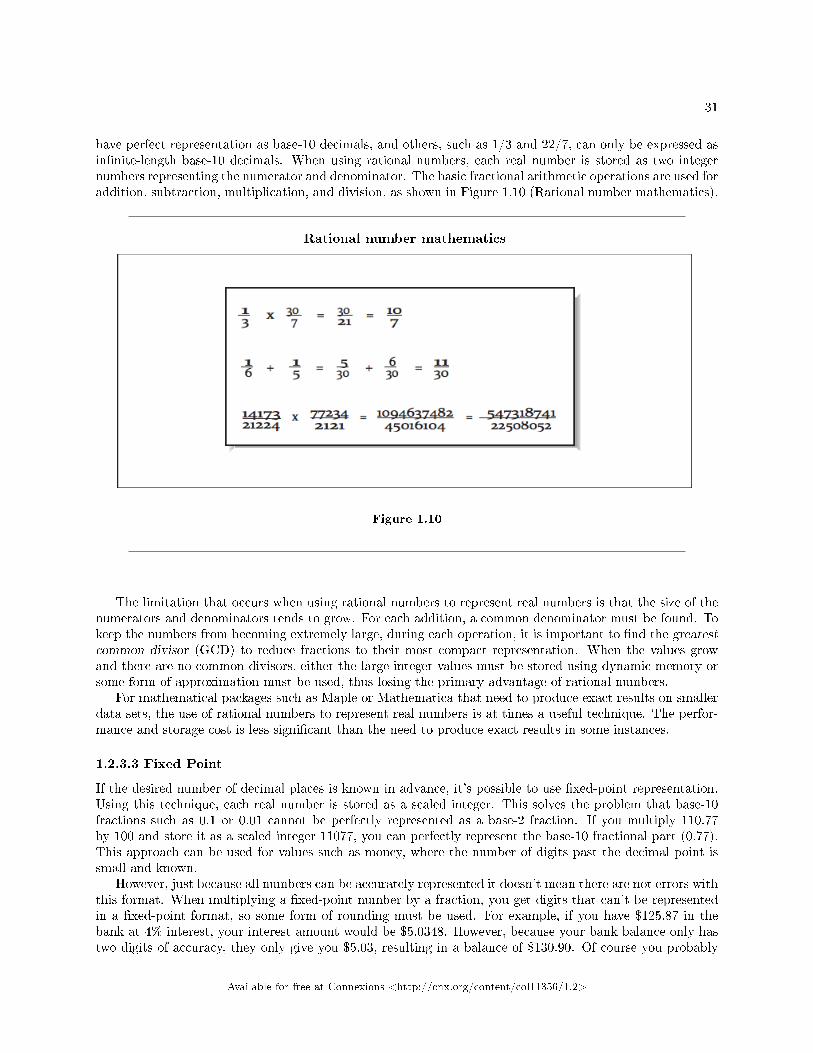
31
have perfect representation as base-10 decimals, and others, such as 1/3 and 22/7, can only be expressed asin�nite-length base-10 decimals. When using rational numbers, each real number is stored as two integernumbers representing the numerator and denominator. The basic fractional arithmetic operations are used foraddition, subtraction, multiplication, and division, as shown in Figure 1.10 (Rational number mathematics).
Rational number mathematics
Figure 1.10
The limitation that occurs when using rational numbers to represent real numbers is that the size of thenumerators and denominators tends to grow. For each addition, a common denominator must be found. Tokeep the numbers from becoming extremely large, during each operation, it is important to �nd the greatestcommon divisor (GCD) to reduce fractions to their most compact representation. When the values growand there are no common divisors, either the large integer values must be stored using dynamic memory orsome form of approximation must be used, thus losing the primary advantage of rational numbers.
For mathematical packages such as Maple or Mathematica that need to produce exact results on smallerdata sets, the use of rational numbers to represent real numbers is at times a useful technique. The perfor-mance and storage cost is less signi�cant than the need to produce exact results in some instances.
1.2.3.3 Fixed Point
If the desired number of decimal places is known in advance, it's possible to use �xed-point representation.Using this technique, each real number is stored as a scaled integer. This solves the problem that base-10fractions such as 0.1 or 0.01 cannot be perfectly represented as a base-2 fraction. If you multiply 110.77by 100 and store it as a scaled integer 11077, you can perfectly represent the base-10 fractional part (0.77).This approach can be used for values such as money, where the number of digits past the decimal point issmall and known.
However, just because all numbers can be accurately represented it doesn't mean there are not errors withthis format. When multiplying a �xed-point number by a fraction, you get digits that can't be representedin a �xed-point format, so some form of rounding must be used. For example, if you have $125.87 in thebank at 4% interest, your interest amount would be $5.0348. However, because your bank balance only hastwo digits of accuracy, they only give you $5.03, resulting in a balance of $130.90. Of course you probably
Available for free at Connexions <http://cnx.org/content/col11356/1.2>
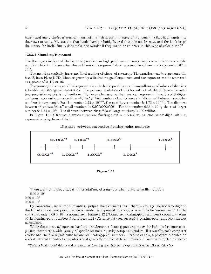
32 CHAPTER 1. ARQUITECTURAS DE CÓMPUTO MODERNAS
have heard many stories of programmers getting rich depositing many of the remaining 0.0048 amounts intotheir own account. My guess is that banks have probably �gured that one out by now, and the bank keepsthe money for itself. But it does make one wonder if they round or truncate in this type of calculation.23
1.2.3.4 Mantissa/Exponent
The �oating-point format that is most prevalent in high performance computing is a variation on scienti�cnotation. In scienti�c notation the real number is represented using a mantissa, base, and exponent: 6.02 ×10²³.
The mantissa typically has some �xed number of places of accuracy. The mantissa can be represented inbase 2, base 16, or BCD. There is generally a limited range of exponents, and the exponent can be expressedas a power of 2, 10, or 16.
The primary advantage of this representation is that it provides a wide overall range of values while usinga �xed-length storage representation. The primary limitation of this format is that the di�erence betweentwo successive values is not uniform. For example, assume that you can represent three base-10 digits,and your exponent can range from �10 to 10. For numbers close to zero, the �distance� between successivenumbers is very small. For the number 1.72× 10⁻¹⁰, the next larger number is 1.73× 10⁻¹⁰. The distancebetween these two �close� small numbers is 0.000000000001. For the number 6.33 × 10¹⁰, the next largernumber is 6.34× 10¹⁰. The distance between these �close� large numbers is 100 million.
In Figure 1.11 (Distance between successive �oating-point numbers), we use two base-2 digits with anexponent ranging from �1 to 1.
Distance between successive �oating-point numbers
Figure 1.11
There are multiple equivalent representations of a number when using scienti�c notation:6.00× 10⁵
0.60× 10⁶
0.06× 10⁷
By convention, we shift the mantissa (adjust the exponent) until there is exactly one nonzero digit tothe left of the decimal point. When a number is expressed this way, it is said to be �normalized.� In theabove list, only 6.00 × 10⁵ is normalized. Figure 1.12 (Normalized �oating-point numbers) shows how someof the �oating-point numbers from Figure 1.11 (Distance between successive �oating-point numbers) are notnormalized.
While the mantissa/exponent has been the dominant �oating-point approach for high performance com-puting, there were a wide variety of speci�c formats in use by computer vendors. Historically, each computervendor had their own particular format for �oating-point numbers. Because of this, a program executed onseveral di�erent brands of computer would generally produce di�erent answers. This invariably led to heated
23Perhaps banks round this instead of truncating, knowing that they will always make it up in teller machine fees.
Available for free at Connexions <http://cnx.org/content/col11356/1.2>
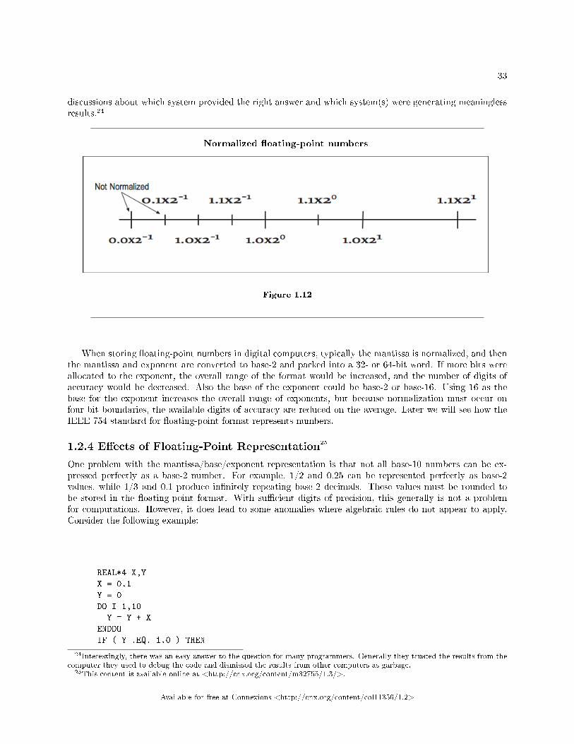
33
discussions about which system provided the right answer and which system(s) were generating meaninglessresults.24
Normalized �oating-point numbers
Figure 1.12
When storing �oating-point numbers in digital computers, typically the mantissa is normalized, and thenthe mantissa and exponent are converted to base-2 and packed into a 32- or 64-bit word. If more bits wereallocated to the exponent, the overall range of the format would be increased, and the number of digits ofaccuracy would be decreased. Also the base of the exponent could be base-2 or base-16. Using 16 as thebase for the exponent increases the overall range of exponents, but because normalization must occur onfour-bit boundaries, the available digits of accuracy are reduced on the average. Later we will see how theIEEE 754 standard for �oating-point format represents numbers.
1.2.4 E�ects of Floating-Point Representation25
One problem with the mantissa/base/exponent representation is that not all base-10 numbers can be ex-pressed perfectly as a base-2 number. For example, 1/2 and 0.25 can be represented perfectly as base-2values, while 1/3 and 0.1 produce in�nitely repeating base-2 decimals. These values must be rounded tobe stored in the �oating-point format. With su�cient digits of precision, this generally is not a problemfor computations. However, it does lead to some anomalies where algebraic rules do not appear to apply.Consider the following example:
REAL*4 X,Y
X = 0.1
Y = 0
DO I=1,10
Y = Y + X
ENDDO
IF ( Y .EQ. 1.0 ) THEN
24Interestingly, there was an easy answer to the question for many programmers. Generally they trusted the results from thecomputer they used to debug the code and dismissed the results from other computers as garbage.
25This content is available online at <http://cnx.org/content/m32755/1.3/>.
Available for free at Connexions <http://cnx.org/content/col11356/1.2>
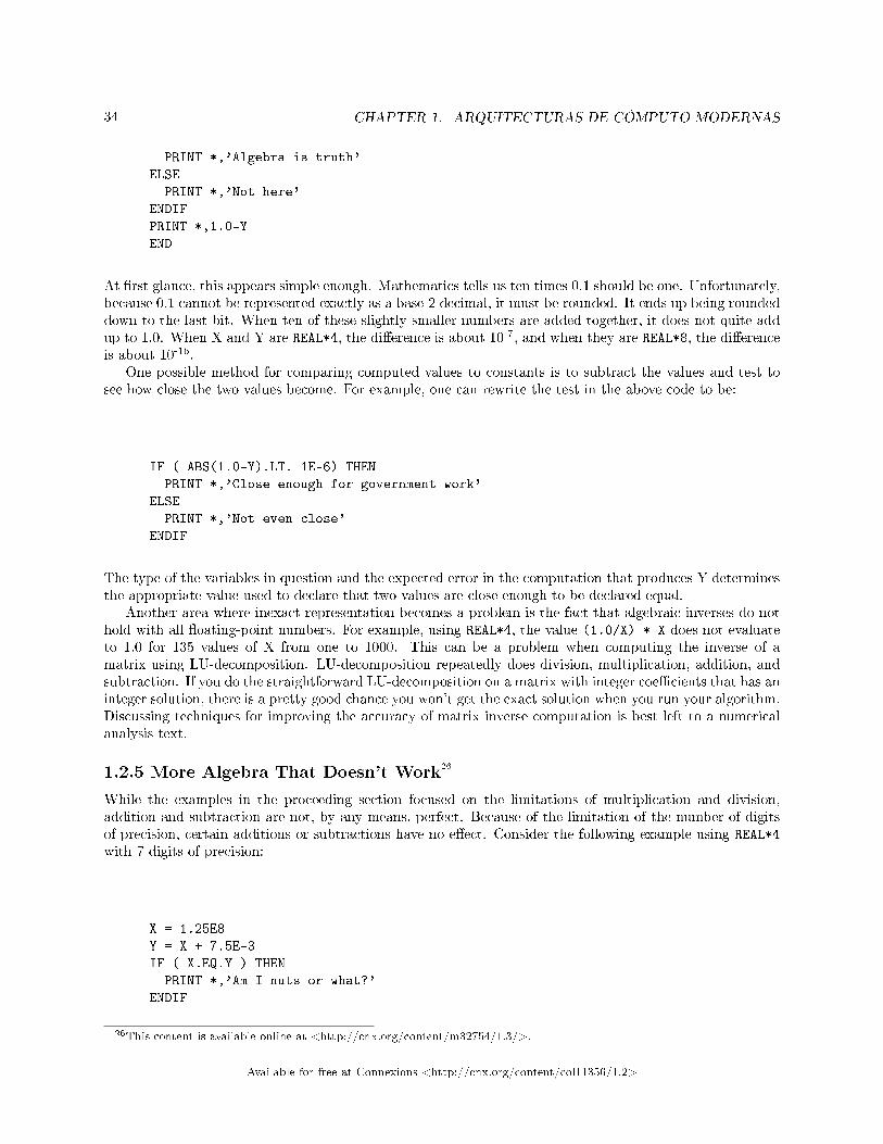
34 CHAPTER 1. ARQUITECTURAS DE CÓMPUTO MODERNAS
PRINT *,'Algebra is truth'
ELSE
PRINT *,'Not here'
ENDIF
PRINT *,1.0-Y
END
At �rst glance, this appears simple enough. Mathematics tells us ten times 0.1 should be one. Unfortunately,because 0.1 cannot be represented exactly as a base-2 decimal, it must be rounded. It ends up being roundeddown to the last bit. When ten of these slightly smaller numbers are added together, it does not quite addup to 1.0. When X and Y are REAL*4, the di�erence is about 10-7, and when they are REAL*8, the di�erenceis about 10-16.
One possible method for comparing computed values to constants is to subtract the values and test tosee how close the two values become. For example, one can rewrite the test in the above code to be:
IF ( ABS(1.0-Y).LT. 1E-6) THEN
PRINT *,'Close enough for government work'
ELSE
PRINT *,'Not even close'
ENDIF
The type of the variables in question and the expected error in the computation that produces Y determinesthe appropriate value used to declare that two values are close enough to be declared equal.
Another area where inexact representation becomes a problem is the fact that algebraic inverses do nothold with all �oating-point numbers. For example, using REAL*4, the value (1.0/X) * X does not evaluateto 1.0 for 135 values of X from one to 1000. This can be a problem when computing the inverse of amatrix using LU-decomposition. LU-decomposition repeatedly does division, multiplication, addition, andsubtraction. If you do the straightforward LU-decomposition on a matrix with integer coe�cients that has aninteger solution, there is a pretty good chance you won't get the exact solution when you run your algorithm.Discussing techniques for improving the accuracy of matrix inverse computation is best left to a numericalanalysis text.
1.2.5 More Algebra That Doesn't Work26
While the examples in the proceeding section focused on the limitations of multiplication and division,addition and subtraction are not, by any means, perfect. Because of the limitation of the number of digitsof precision, certain additions or subtractions have no e�ect. Consider the following example using REAL*4
with 7 digits of precision:
X = 1.25E8
Y = X + 7.5E-3
IF ( X.EQ.Y ) THEN
PRINT *,'Am I nuts or what?'
ENDIF
26This content is available online at <http://cnx.org/content/m32754/1.3/>.
Available for free at Connexions <http://cnx.org/content/col11356/1.2>
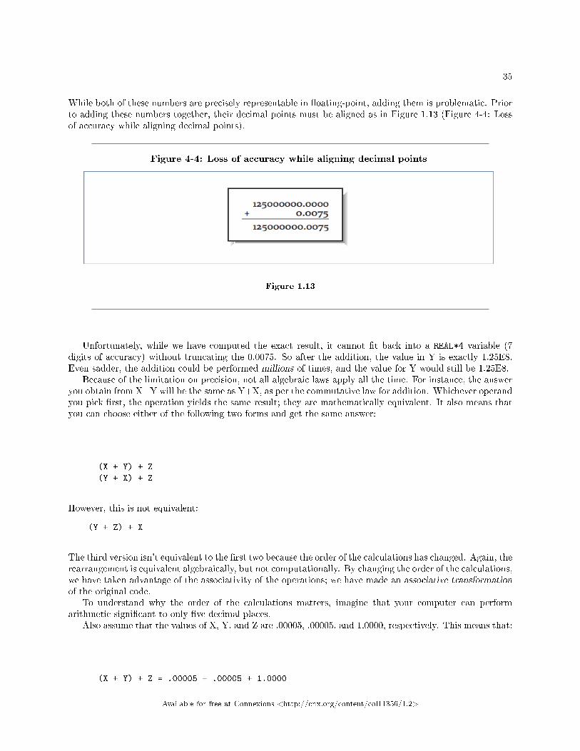
35
While both of these numbers are precisely representable in �oating-point, adding them is problematic. Priorto adding these numbers together, their decimal points must be aligned as in Figure 1.13 (Figure 4-4: Lossof accuracy while aligning decimal points).
Figure 4-4: Loss of accuracy while aligning decimal points
Figure 1.13
Unfortunately, while we have computed the exact result, it cannot �t back into a REAL*4 variable (7digits of accuracy) without truncating the 0.0075. So after the addition, the value in Y is exactly 1.25E8.Even sadder, the addition could be performed millions of times, and the value for Y would still be 1.25E8.
Because of the limitation on precision, not all algebraic laws apply all the time. For instance, the answeryou obtain from X+Y will be the same as Y+X, as per the commutative law for addition. Whichever operandyou pick �rst, the operation yields the same result; they are mathematically equivalent. It also means thatyou can choose either of the following two forms and get the same answer:
(X + Y) + Z
(Y + X) + Z
However, this is not equivalent:
(Y + Z) + X
The third version isn't equivalent to the �rst two because the order of the calculations has changed. Again, therearrangement is equivalent algebraically, but not computationally. By changing the order of the calculations,we have taken advantage of the associativity of the operations; we have made an associative transformationof the original code.
To understand why the order of the calculations matters, imagine that your computer can performarithmetic signi�cant to only �ve decimal places.
Also assume that the values of X, Y, and Z are .00005, .00005, and 1.0000, respectively. This means that:
(X + Y) + Z = .00005 + .00005 + 1.0000
Available for free at Connexions <http://cnx.org/content/col11356/1.2>

36 CHAPTER 1. ARQUITECTURAS DE CÓMPUTO MODERNAS
= .0001 + 1.0000 = 1.0001
but:
(Y + Z) + X = .00005 + 1.0000 + .00005
= 1.0000 + .00005 = 1.0000
The two versions give slightly di�erent answers. When adding Y+Z+X, the sum of the smaller numbers wasinsigni�cant when added to the larger number. But when computing X+Y+Z, we add the two small numbers�rst, and their combined sum is large enough to in�uence the �nal answer. For this reason, compilersthat rearrange operations for the sake of performance generally only do so after the user has requestedoptimizations beyond the defaults.
For these reasons, the FORTRAN language is very strict about the exact order of evaluation of ex-pressions. To be compliant, the compiler must ensure that the operations occur exactly as you expressthem.27
For Kernighan and Ritchie C, the operator precedence rules are di�erent. Although the precedencesbetween operators are honored (i.e., * comes before +, and evaluation generally occurs left to right foroperators of equal precedence), the compiler is allowed to treat a few commutative operations (+, *, &, �and |) as if they were fully associative, even if they are parenthesized. For instance, you might tell the Ccompiler:
a = x + (y + z);
However, the C compiler is free to ignore you, and combine X, Y, and Z in any order it pleases.Now armed with this knowledge, view the following harmless-looking code segment:
REAL*4 SUM,A(1000000)
SUM = 0.0
DO I=1,1000000
SUM = SUM + A(I)
ENDDO
Begins to look like a nightmare waiting to happen. The accuracy of this sum depends of the relativemagnitudes and order of the values in the array A. If we sort the array from smallest to largest and thenperform the additions, we have a more accurate value. There are other algorithms for computing the sumof an array that reduce the error without requiring a full sort of the data. Consult a good textbook onnumerical analysis for the details on these algorithms.
If the range of magnitudes of the values in the array is relatively small, the straight- forward computationof the sum is probably su�cient.
27Often even if you didn't mean it.
Available for free at Connexions <http://cnx.org/content/col11356/1.2>

37
1.2.6 Improving Accuracy Using Guard Digits28
In this section we explore a technique to improve the precision of �oating-point computations without usingadditional storage space for the �oating-point numbers.
Consider the following example of a base-10 system with �ve digits of accuracy performing the followingsubtraction:
10.001 - 9.9993 = 0.0017
All of these values can be perfectly represented using our �oating-point format. However, if we only have�ve digits of precision available while aligning the decimal points during the computation, the results endup with signi�cant error as shown in Figure 1.14 (Need for guard digits ).
Need for guard digits
Figure 1.14
To perform this computation and round it correctly, we do not need to increase the number of signi�cantdigits for stored values. We do, however, need additional digits of precision while performing the computation.
The solution is to add extra guard digits which are maintained during the interim steps of the compu-tation. In our case, if we maintained six digits of accuracy while aligning operands, and rounded beforenormalizing and assigning the �nal value, we would get the proper result. The guard digits only need to bepresent as part of the �oating-point execution unit in the CPU. It is not necessary to add guard digits tothe registers or to the values stored in memory.
It is not necessary to have an extremely large number of guard digits. At some point, the di�erence inthe magnitude between the operands becomes so great that lost digits do not a�ect the addition or roundingresults.
1.2.7 History of IEEE Floating-Point Format29
1.2.7.1 History of IEEE Floating-Point Format
Prior to the RISC microprocessor revolution, each vendor had their own �oating- point formats based ontheir designers' views of the relative importance of range versus accuracy and speed versus accuracy. It wasnot uncommon for one vendor to carefully analyze the limitations of another vendor's �oating-point formatand use this information to convince users that theirs was the only �accurate� �oating- point implementation.In reality none of the formats was perfect. The formats were simply imperfect in di�erent ways.
During the 1980s the Institute for Electrical and Electronics Engineers (IEEE) produced a standard forthe �oating-point format. The title of the standard is �IEEE 754-1985 Standard for Binary Floating-Point
28This content is available online at <http://cnx.org/content/m32744/1.3/>.29This content is available online at <http://cnx.org/content/m32770/1.3/>.
Available for free at Connexions <http://cnx.org/content/col11356/1.2>
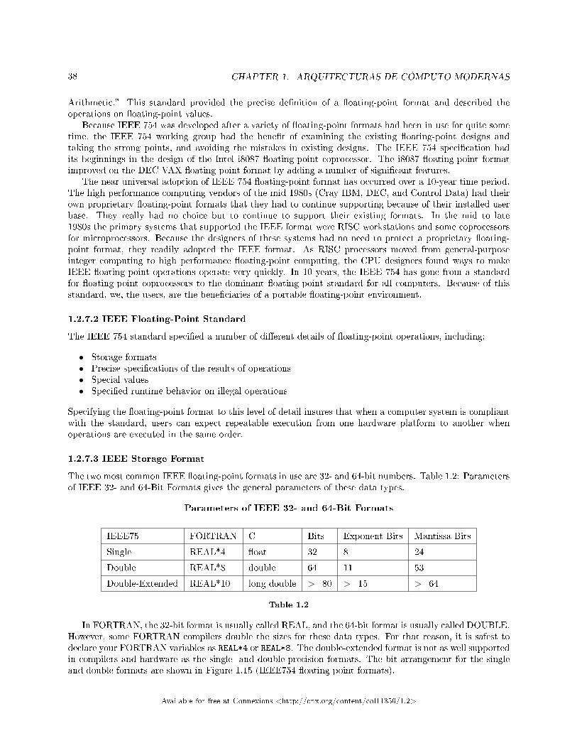
38 CHAPTER 1. ARQUITECTURAS DE CÓMPUTO MODERNAS
Arithmetic.� This standard provided the precise de�nition of a �oating-point format and described theoperations on �oating-point values.
Because IEEE 754 was developed after a variety of �oating-point formats had been in use for quite sometime, the IEEE 754 working group had the bene�t of examining the existing �oating-point designs andtaking the strong points, and avoiding the mistakes in existing designs. The IEEE 754 speci�cation hadits beginnings in the design of the Intel i8087 �oating-point coprocessor. The i8087 �oating-point formatimproved on the DEC VAX �oating-point format by adding a number of signi�cant features.
The near universal adoption of IEEE 754 �oating-point format has occurred over a 10-year time period.The high performance computing vendors of the mid 1980s (Cray IBM, DEC, and Control Data) had theirown proprietary �oating-point formats that they had to continue supporting because of their installed userbase. They really had no choice but to continue to support their existing formats. In the mid to late1980s the primary systems that supported the IEEE format were RISC workstations and some coprocessorsfor microprocessors. Because the designers of these systems had no need to protect a proprietary �oating-point format, they readily adopted the IEEE format. As RISC processors moved from general-purposeinteger computing to high performance �oating-point computing, the CPU designers found ways to makeIEEE �oating-point operations operate very quickly. In 10 years, the IEEE 754 has gone from a standardfor �oating-point coprocessors to the dominant �oating-point standard for all computers. Because of thisstandard, we, the users, are the bene�ciaries of a portable �oating-point environment.
1.2.7.2 IEEE Floating-Point Standard
The IEEE 754 standard speci�ed a number of di�erent details of �oating-point operations, including:
• Storage formats• Precise speci�cations of the results of operations• Special values• Speci�ed runtime behavior on illegal operations
Specifying the �oating-point format to this level of detail insures that when a computer system is compliantwith the standard, users can expect repeatable execution from one hardware platform to another whenoperations are executed in the same order.
1.2.7.3 IEEE Storage Format
The two most common IEEE �oating-point formats in use are 32- and 64-bit numbers. Table 1.2: Parametersof IEEE 32- and 64-Bit Formats gives the general parameters of these data types.
Parameters of IEEE 32- and 64-Bit Formats
IEEE75 FORTRAN C Bits Exponent Bits Mantissa Bits
Single REAL*4 �oat 32 8 24
Double REAL*8 double 64 11 53
Double-Extended REAL*10 long double >=80 >=15 >=64
Table 1.2
In FORTRAN, the 32-bit format is usually called REAL, and the 64-bit format is usually called DOUBLE.However, some FORTRAN compilers double the sizes for these data types. For that reason, it is safest todeclare your FORTRAN variables as REAL*4 or REAL*8. The double-extended format is not as well supportedin compilers and hardware as the single- and double-precision formats. The bit arrangement for the singleand double formats are shown in Figure 1.15 (IEEE754 �oating-point formats).
Available for free at Connexions <http://cnx.org/content/col11356/1.2>
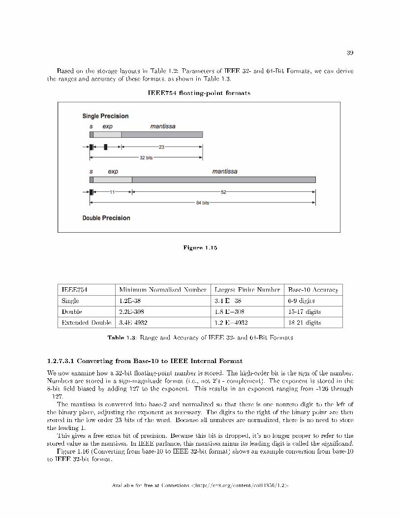
39
Based on the storage layouts in Table 1.2: Parameters of IEEE 32- and 64-Bit Formats, we can derivethe ranges and accuracy of these formats, as shown in Table 1.3.
IEEE754 �oating-point formats
Figure 1.15
IEEE754 Minimum Normalized Number Largest Finite Number Base-10 Accuracy
Single 1.2E-38 3.4 E+38 6-9 digits
Double 2.2E-308 1.8 E+308 15-17 digits
Extended Double 3.4E-4932 1.2 E+4932 18-21 digits
Table 1.3: Range and Accuracy of IEEE 32- and 64-Bit Formats
1.2.7.3.1 Converting from Base-10 to IEEE Internal Format
We now examine how a 32-bit �oating-point number is stored. The high-order bit is the sign of the number.Numbers are stored in a sign-magnitude format (i.e., not 2's - complement). The exponent is stored in the8-bit �eld biased by adding 127 to the exponent. This results in an exponent ranging from -126 through+127.
The mantissa is converted into base-2 and normalized so that there is one nonzero digit to the left ofthe binary place, adjusting the exponent as necessary. The digits to the right of the binary point are thenstored in the low-order 23 bits of the word. Because all numbers are normalized, there is no need to storethe leading 1.
This gives a free extra bit of precision. Because this bit is dropped, it's no longer proper to refer to thestored value as the mantissa. In IEEE parlance, this mantissa minus its leading digit is called the signi�cand.
Figure 1.16 (Converting from base-10 to IEEE 32-bit format) shows an example conversion from base-10to IEEE 32-bit format.
Available for free at Connexions <http://cnx.org/content/col11356/1.2>
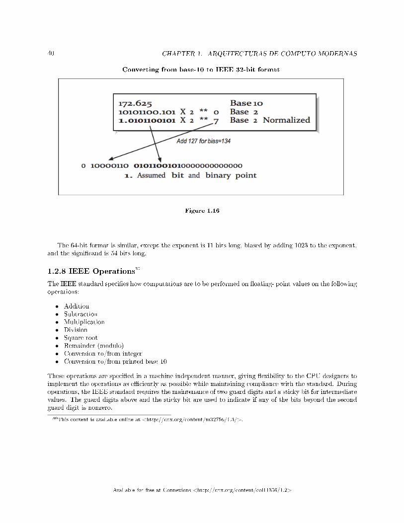
40 CHAPTER 1. ARQUITECTURAS DE CÓMPUTO MODERNAS
Converting from base-10 to IEEE 32-bit format
Figure 1.16
The 64-bit format is similar, except the exponent is 11 bits long, biased by adding 1023 to the exponent,and the signi�cand is 54 bits long.
1.2.8 IEEE Operations30
The IEEE standard speci�es how computations are to be performed on �oating- point values on the followingoperations:
• Addition• Subtraction• Multiplication• Division• Square root• Remainder (modulo)• Conversion to/from integer• Conversion to/from printed base-10
These operations are speci�ed in a machine-independent manner, giving �exibility to the CPU designers toimplement the operations as e�ciently as possible while maintaining compliance with the standard. Duringoperations, the IEEE standard requires the maintenance of two guard digits and a sticky bit for intermediatevalues. The guard digits above and the sticky bit are used to indicate if any of the bits beyond the secondguard digit is nonzero.
30This content is available online at <http://cnx.org/content/m32756/1.3/>.
Available for free at Connexions <http://cnx.org/content/col11356/1.2>

41
Computation using guard and sticky bits
Figure 1.17
In Figure 1.17 (Computation using guard and sticky bits), we have �ve bits of normal precision, twoguard digits, and a sticky bit. Guard bits simply operate as normal bits � as if the signi�cand were 25bits. Guard bits participate in rounding as the extended operands are added. The sticky bit is set to 1 ifany of the bits beyond the guard bits is nonzero in either operand.31 Once the extended sum is computed,it is rounded so that the value stored in memory is the closest possible value to the extended sum includingthe guard digits. Table 1.4 shows all eight possible values of the two guard digits and the sticky bit and theresulting stored value with an explanation as to why.
31If you are somewhat hardware-inclined and you think about it for a moment, you will soon come up with a way to properlymaintain the sticky bit without ever computing the full �in�nite precision sum.� You just have to keep track as things getshifted around.
Available for free at Connexions <http://cnx.org/content/col11356/1.2>
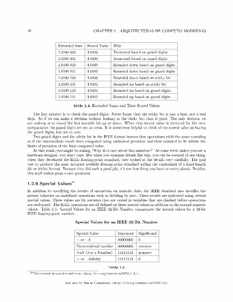
42 CHAPTER 1. ARQUITECTURAS DE CÓMPUTO MODERNAS
Extended Sum Stored Value Why
1.0100 000 1.0100 Truncated based on guard digits
1.0100 001 1.0100 Truncated based on guard digits
1.0100 010 1.0100 Rounded down based on guard digits
1.0100 011 1.0100 Rounded down based on guard digits
1.0100 100 1.0100 Rounded down based on sticky bit
1.0100 101 1.0101 Rounded up based on sticky bit
1.0100 110 1.0101 Rounded up based on guard digits
1.0100 111 1.0101 Rounded up based on guard digits
Table 1.4: Extended Sums and Their Stored Values
The �rst priority is to check the guard digits. Never forget that the sticky bit is just a hint, not a realdigit. So if we can make a decision without looking at the sticky bit, that is good. The only decision weare making is to round the last storable bit up or down. When that stored value is retrieved for the nextcomputation, its guard digits are set to zeros. It is sometimes helpful to think of the stored value as havingthe guard digits, but set to zero.
Two guard digits and the sticky bit in the IEEE format insures that operations yield the same roundingas if the intermediate result were computed using unlimited precision and then rounded to �t within thelimits of precision of the �nal computed value.
At this point, you might be asking, �Why do I care about this minutiae?� At some level, unless you are ahardware designer, you don't care. But when you examine details like this, you can be assured of one thing:when they developed the IEEE �oating-point standard, they looked at the details very carefully. The goalwas to produce the most accurate possible �oating-point standard within the constraints of a �xed-length32- or 64-bit format. Because they did such a good job, it's one less thing you have to worry about. Besides,this stu� makes great exam questions.
1.2.9 Special Values32
In addition to specifying the results of operations on numeric data, the IEEE standard also speci�es theprecise behavior on unde�ned operations such as dividing by zero. These results are indicated using severalspecial values. These values are bit patterns that are stored in variables that are checked before operationsare performed. The IEEE operations are all de�ned on these special values in addition to the normal numericvalues. Table 1.5: Special Values for an IEEE 32-Bit Number summarizes the special values for a 32-bitIEEE �oating-point number.
Special Values for an IEEE 32-Bit Number
Special Value Exponent Signi�cand
+ or � 0 00000000 0
Denormalized number 00000000 nonzero
NaN (Not a Number) 11111111 nonzero
+ or � In�nity 11111111 0
Table 1.5
32This content is available online at <http://cnx.org/content/m32758/1.3/>.
Available for free at Connexions <http://cnx.org/content/col11356/1.2>

43
The value of the exponent and signi�cand determines which type of special value this particular �oating-point number represents. Zero is designed such that integer zero and �oating-point zero are the same bitpattern.
Denormalized numbers can occur at some point as a number continues to get smaller, and the exponenthas reached the minimum value. We could declare that minimum to be the smallest representable value.However, with denormalized values, we can continue by setting the exponent bits to zero and shifting thesigni�cand bits to the right, �rst adding the leading �1� that was dropped, then continuing to add leadingzeros to indicate even smaller values. At some point the last nonzero digit is shifted o� to the right, and thevalue becomes zero. This approach is called gradual under�ow where the value keeps approaching zero andthen eventually becomes zero. Not all implementations support denormalized numbers in hardware; theymight trap to a software routine to handle these numbers at a signi�cant performance cost.
At the top end of the biased exponent value, an exponent of all 1s can represent the Not a Number(NaN) value or in�nity. In�nity occurs in computations roughly according to the principles of mathematics.If you continue to increase the magnitude of a number beyond the range of the �oating-point format, oncethe range has been exceeded, the value becomes in�nity. Once a value is in�nity, further additions won'tincrease it, and subtractions won't decrease it. You can also produce the value in�nity by dividing a nonzerovalue by zero. If you divide a nonzero value by in�nity, you get zero as a result.
The NaN value indicates a number that is not mathematically de�ned. You can generate a NaN bydividing zero by zero, dividing in�nity by in�nity, or taking the square root of -1. The di�erence betweenin�nity and NaN is that the NaN value has a nonzero signi�cand. The NaN value is very sticky. Anyoperation that has a NaN as one of its inputs always produces a NaN result.
1.2.10 Exceptions and Traps33
In addition to de�ning the results of computations that aren't mathematically de�ned, the IEEE standardprovides programmers with the ability to detect when these special values are being produced. This way,programmers can write their code without adding extensive IF tests throughout the code checking for themagnitude of values. Instead they can register a trap handler for an event such as under�ow and handle theevent when it occurs. The exceptions de�ned by the IEEE standard include:
• Over�ow to in�nity• Under�ow to zero• Division by zero• Invalid operation• Inexact operation
According to the standard, these traps are under the control of the user. In most cases, the compiler runtimelibrary manages these traps under the direction from the user through compiler �ags or runtime library calls.Traps generally have signi�cant overhead compared to a single �oating-point instruction, and if a programis continually executing trap code, it can signi�cantly impact performance.
In some cases it's appropriate to ignore traps on certain operations. A commonly ignored trap is theunder�ow trap. In many iterative programs, it's quite natural for a value to keep reducing to the point whereit �disappears.� Depending on the application, this may or may not be an error situation so this exceptioncan be safely ignored.
If you run a program and then it terminates, you see a message such as:
Overflow handler called 10,000,000 times
It probably means that you need to �gure out why your code is exceeding the range of the �oating-pointformat. It probably also means that your code is executing more slowly because it is spending too muchtime in its error handlers.
33This content is available online at <http://cnx.org/content/m32760/1.3/>.
Available for free at Connexions <http://cnx.org/content/col11356/1.2>

44 CHAPTER 1. ARQUITECTURAS DE CÓMPUTO MODERNAS
1.2.11 Compiler Issues34
The IEEE 754 �oating-point standard does a good job describing how �oating- point operations are to beperformed. However, we generally don't write assembly language programs. When we write in a higher-levellanguage such as FORTRAN, it's sometimes di�cult to get the compiler to generate the assembly languageyou need for your application. The problems fall into two categories:
• The compiler is too conservative in trying to generate IEEE-compliant code and produces code thatdoesn't operate at the peak speed of the processor. On some processors, to fully support gradual under-�ow, extra instructions must be generated for certain instructions. If your code will never under�ow,these instructions are unnecessary overhead.
• The optimizer takes liberties rewriting your code to improve its performance, eliminating some neces-sary steps. For example, if you have the following code:
Z = X + 500
Y = Z - 200
The optimizer may replace it with Y = X + 300. However, in the case of a value for X that is close toover�ow, the two sequences may not produce the same result.
Sometimes a user prefers �fast� code that loosely conforms to the IEEE standard, and at other times theuser will be writing a numerical library routine and need total control over each �oating-point operation.Compilers have a challenge supporting the needs of both of these types of users. Because of the nature ofthe high performance computing market and benchmarks, often the �fast and loose� approach prevails inmany compilers.
1.2.12 Closing Notes35
While this is a relatively long chapter with a lot of technical detail, it does not even begin to scratch thesurface of the IEEE �oating-point format or the entire �eld of numerical analysis. We as programmers mustbe careful about the accuracy of our programs, lest the results become meaningless. Here are a few basicrules to get you started:
• Look for compiler options that relax or enforce strict IEEE compliance and choose the appropriateoption for your program. You may even want to change these options for di�erent portions of yourprogram.
• Use REAL*8 for computations unless you are sure REAL*4 has su�cient precision. Given that REAL*4has roughly 7 digits of precision, if the bottom digits become meaningless due to rounding and compu-tations, you are in some danger of seeing the e�ect of the errors in your results. REAL*8 with 13 digitsmakes this much less likely to happen.
• Be aware of the relative magnitude of numbers when you are performing additions.• When summing up numbers, if there is a wide range, sum from smallest to largest.• Perform multiplications before divisions whenever possible.• When performing a comparison with a computed value, check to see if the values are �close� rather
than identical.• Make sure that you are not performing any unnecessary type conversions during the critical portions
of your code.
34This content is available online at <http://cnx.org/content/m32762/1.3/>.35This content is available online at <http://cnx.org/content/m32768/1.3/>.
Available for free at Connexions <http://cnx.org/content/col11356/1.2>
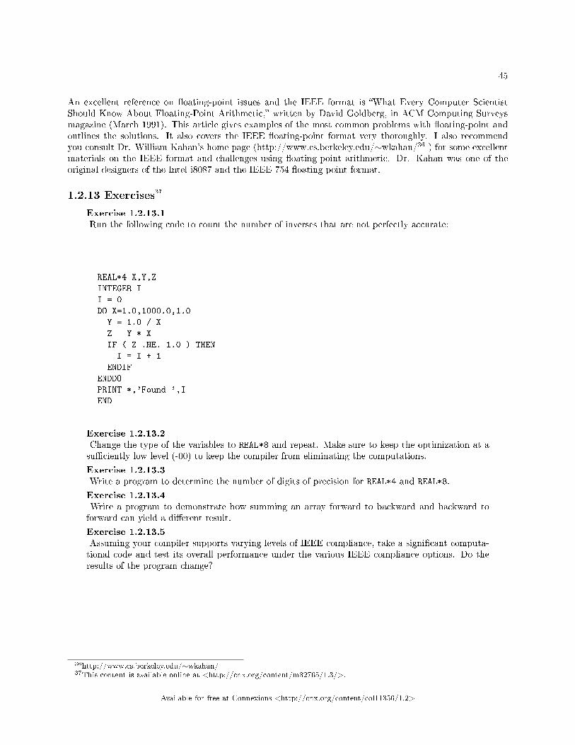
45
An excellent reference on �oating-point issues and the IEEE format is �What Every Computer ScientistShould Know About Floating-Point Arithmetic,� written by David Goldberg, in ACM Computing Surveysmagazine (March 1991). This article gives examples of the most common problems with �oating-point andoutlines the solutions. It also covers the IEEE �oating-point format very thoroughly. I also recommendyou consult Dr. William Kahan's home page (http://www.cs.berkeley.edu/∼wkahan/36 ) for some excellentmaterials on the IEEE format and challenges using �oating-point arithmetic. Dr. Kahan was one of theoriginal designers of the Intel i8087 and the IEEE 754 �oating-point format.
1.2.13 Exercises37
Exercise 1.2.13.1Run the following code to count the number of inverses that are not perfectly accurate:
REAL*4 X,Y,Z
INTEGER I
I = 0
DO X=1.0,1000.0,1.0
Y = 1.0 / X
Z = Y * X
IF ( Z .NE. 1.0 ) THEN
I = I + 1
ENDIF
ENDDO
PRINT *,'Found ',I
END
Exercise 1.2.13.2Change the type of the variables to REAL*8 and repeat. Make sure to keep the optimization at asu�ciently low level (-00) to keep the compiler from eliminating the computations.
Exercise 1.2.13.3Write a program to determine the number of digits of precision for REAL*4 and REAL*8.
Exercise 1.2.13.4Write a program to demonstrate how summing an array forward to backward and backward toforward can yield a di�erent result.
Exercise 1.2.13.5Assuming your compiler supports varying levels of IEEE compliance, take a signi�cant computa-tional code and test its overall performance under the various IEEE compliance options. Do theresults of the program change?
36http://www.cs.berkeley.edu/∼wkahan/37This content is available online at <http://cnx.org/content/m32765/1.3/>.
Available for free at Connexions <http://cnx.org/content/col11356/1.2>

46 CHAPTER 1. ARQUITECTURAS DE CÓMPUTO MODERNAS
Available for free at Connexions <http://cnx.org/content/col11356/1.2>
Chapter 2
Programando y A�nando Software
2.1 Qué Hace un Compilador
2.1.1 Qué Hace un Compilador - Introducción1
2.1.1.1 Lo que Hace un Compilador
El objetivo de un compilador optimizador es la traducción e�ciente de un lenguaje de alto nivel al lenguajemáquina más rápido posible, que represente con precisión al primero. Lo que hace buena a una representaciónes: da las respuestas correctas, y se ejecuta rápidamente.
Naturalmente, no importa cuán rápido se ejecute un programa si no produce las respuestas correctas.2
Pero dada una expresión de un programa que se ejecuta correctamente, un compilador optimizador buscaformas de acelerarla. En primera instancia usualmente signi�ca simpli�car el código, retirando instruccionesextrañas, y compartiendo los resultados intermedios entre sentencias. Algunas optimizaciones más avanzadasbuscan reestructurar el programa, a veces incrementando el tamaño del código, aunque (con algo de fortuna)el número de instrucciones ejecutadas se reduzca.
Cuando llegue �nalmente el momento de generar lenguaje máquina, el compilador debe saber acerca de losregistros y las reglas para emitir instrucciones. Para lograr alto desempeño, requiere entender el costo de talesinstrucciones y las latencias de los recursos de la máquina, tales como las �las de espera. Esto es especialmentecierto para aquellos procesadores que pueden ejecutar más de una instrucción simultáneamente. Se necesitade una mezcla balanceada de instrucciones -la proporción correcta de operaciones de punto �otante, punto�jo, memoria, saltos, etc.- para mantener a la máquina ocupada.
Inicialmente los compiladores eran herramientas que nos permitían escribir en algo más legible que ellenguaje ensamblador. Hoy en día rondan la inteligencia arti�cial, conforme toman nuestro código fuente dealto nivel y lo traducen a una versión altamente optimizada de lenguaje máquina, a través de una ampliavariedad de arquitecturas uniprocesador y multiprocesador. En el área del cómputo de alto rendimiento, amenudo sucede que el compilador tiene un impacto mayor sobre el desempeño de nuestro programa que lasarquitecturas del procesador o de la memoria. A lo largo de la historia del cómputo de alto rendimiento hasucedido que, si no estábamos satisfechos con el desempeño de nuestro programa escrito en un lenguaje dealto nivel, alegremente reescribíamos todo o parte del mismo en lenguaje ensamblador. Afortunadamente,los compiladores actuales usualmente hacen este paso innecesario.
En este capítulo cubriremos la operación básica de los compiladores optimizadores. En un capítuloposterior cubriremos las técnicas usadas para analizar y compilar programas para arquitecturas avanzadas,tales como los sistemas paralelos o de procesamiento vectorial. Iniciaremos nuestra revisión de los compi-ladores, examinando cómo ha ido cambiando a lo largo del tiempo la relación entre los programadores y suscompiladores.
1This content is available online at <http://cnx.org/content/m38387/1.2/>.2Sin embargo, a menudo se troca precisión por velocidad.
Available for free at Connexions <http://cnx.org/content/col11356/1.2>
47
48 CHAPTER 2. PROGRAMANDO Y AFINANDO SOFTWARE
2.1.2 Qué Hace un Compilador - Historia de los Compiladores3
Si usted ha formado parte del mundo del cómputo de alto rendimiento desde sus inicios en la década de 1950,le ha tocado programar en varios lenguajes desde entonces. Durante la década de 1950 e inicios de la de 1960,lo hizo en lenguaje ensamblador. La escasez de memoria y las bajas velocidades de reloj hacían que cadainstrucción fuera preciosa. Con pequeñas memorias, el tamaño de los programas era típicamente pequeño,así que con el lenguaje ensamblador era su�ciente. Para �nales de la década de 1960, los programadorescomenzaron a escribir más código en un lenguaje de alto nivel como FORTRAN. Usar uno de tales lenguajeshace que el trabajo que usted realice sea más transportable, con�able y fácil de mantener. Dado el incrementoen velocidad y capacidad de las computadoras, el costo de usar un lenguaje de alto nivel fue algo que lamayoría de los programadores estaban dispuestos a aceptar. En la década de 1970, si un programa gastabauna cantidad particularmente grande de tiempo en cierta rutina, o la rutina formaba parte del sistemaoperativo, o se trataba de una biblioteca de uso común, muy probablemente estuviera escrita en ensamblador.
Durante la última parte de la década de 1970 e inicios de la de 1980, los compiladores optimizadorescontinuaron mejorando hasta el punto en que el grueso de los programas de propósito general, exceptolas porciones más críticas, se escribían en lenguajes de alto nivel. En promedio, los compiladores generanmejor código que la mayoría de los programadores humanos de ensamblador. A menudo ello se debe aque el compilador puede hacer un mejor uso de algunos recursos de hardware, tales como los registros. Enun procesador con 16 registros, un programador debe adoptar alguna convención respecto a qué registrosusar para cada cosa, con el �n de poder seguirle la pista al valor que cada uno almacena. Un compiladorpuede usar cada registro como le plazca, porque puede darle un seguimiento preciso al momento en que estádisponible para otro uso.
Sin embargo, durante ese periodo, también evolucionó la arquitectura de las computadoras de altorendimiento. Cray Research estaba desarrollando procesadores vectoriales en el extremo superior del es-pectro computacional. Los compiladores todavía no estaban listos para determinar cuándo debían emplearesas nuevas instrucciones vectoriales. Los programadores se vieron forzados a escribir lenguaje ensambladoro crear código FORTRAN muy a�nado que invocaba a las rutinas vectoriales apropiadas en su código. Encierto sentido, los procesadores vectoriales hicieron girar las manecillas del reloj en el sentido inverso, hastaque comenzaron a con�ar en el compilador. Los programadores nunca regresaron completamente al lenguajeensamblador, pero su código FORTRAN comenzaba a lucir más como no-FORTRAN. Conforme maduraronlas computadoras vectoriales, sus compiladores fueron progresivamente capaces de detectar cuándo podíarealizarse la vectorización. Y en algún momento nuevamente se hicieron mejores que los programadoreshumanos en tales arquitecturas. Los nuevos compiladores reducían la necesidad de usar intensivamentedirectivas o extensiones del lenguaje.4
La revolución RISC descansaba en una dependencia creciente respecto al compilador. Programar en losprimeros procesadores RISC, tales como el Intel i860 resultaba doloroso si se comparaba con los procesadoresCISC. Sutiles diferencias en la forma de codi�car un programa en lenguaje máquina podían tener un impactosigni�cativo en el rendimiento global del programa. Por ejemplo, un programador debía contar los ciclostranscurridos entre una instrucción de carga y el uso de los resultados de la carga en una instrucción posteriorde cálculo. Conforme se desarrollaron procesadores superescalares, se hizo necesario volver simultáneasciertos pares de instrucciones, y otras debían acomodarse secuencialmente. Dado que había en el mercadoun gran número de procesadores RISC distintos, los programadores no tenían tiempo de aprender talesparticularidades para lograr hasta la última gota de rendimiento en cada procesador. Era más fácil mantenerunidos al diseñador del procesador y el escritor del compilador (que con suerte trabajaban para la mismacompañía) y hacer que discutieran a fondo la mejor forma de generar el código máquina. Y entoncescualquiera podía usar el compilador y obtener código que hiciera un uso razonablemente bueno del hardware.
El compilador se convirtió en una herramienta importante en el ciclo de diseño del procesador. Losdiseñadores de procesadores tenían mucha mayor �exibilidad respecto a los tipos de cambios que podían
3This content is available online at <http://cnx.org/content/m38391/1.2/>.4Los Ciclos de Livermore eran una prueba comparativa que especí�camente comprobaba la capacidad del compilador para
optimizar e�cientemente un conjunto de ciclos. Además de ser una prueba comparativa de rendimiento, también comparabalos compiladores.
Available for free at Connexions <http://cnx.org/content/col11356/1.2>
49
hacer. Por ejemplo, podía suceder que un buen diseño en la siguiente revisión de un procesador ejecutasecódigo previo 10% más lento que una revisión nueva, pero recompilando el código lo hiciera 65% más rápido.Por supuesto, era importante proporcionar dicho compilador con cada nuevo embarque de procesadores, yque dicho compilador diera ese nivel de rendimiento en una amplia variedad de código, y no sólo en una suitede pruebas de escritorio en particular.
2.1.3 Qué Hace un Compilador - Cuál Lenguaje Optimizar5
Se ha dicho, "No sé qué lenguaje se usará para programar computadoras de alto rendimiento dentro de10 años, pero sí que se llamará FORTRAN". A riesgo de iniciar una guerra de exterminio, necesitamosdiscutir las fortalezas y debilidades de los lenguajes que se usan para cómputo de alto rendimiento. Muchoscientí�cos de computadoras (no cientí�cos de la computación) se han entrenado en una dieta continua de C,C++6 o algún otro lenguaje enfocado en estructuras de datos u objetos. Cuando los estudiantes se topanpor vez primera con el cómputo de alto rendimiento, tienen el deseo instintivo de continuar programandoen su lenguaje favorito. Sin embargo, si se quiere obtener el rendimiento máximo en un extenso rango dearquitecturas, FORTRAN es el único lenguaje práctico.
Cuando los estudiantes preguntan el porqué, usualmente la primera respuesta es "porque siempre hasido así". Y en cierta forma es cierto. Físicos, ingenieros mecánicos, químicos, ingenieros estructurales ymeteorólogos realizan mucha programación en computadoras de alto rendimiento, y FORTRAN es el lenguajeen esos campos. (¾Cuándo fue la última vez que un estudiante de ciencias de la computación escribió unprograma que funcione apropiadamente, y que calcule durante una semana completa?) Así que de formanatural los vendedores de computadoras de alto rendimiento ponen un gran esfuerzo en hacer que FORTRANtrabaje muy bien en la arquitectura que comercializan.
Pero, claro está, ésta no es la única razón por la cual FORTRAN es el mejor lenguaje. Hay algunoselementos fundamentales que hacen que C, C++ o cualesquiera otro lenguaje orientado a las estructurasde datos no resulte adecuado para la programación de alto rendimiento. En una palabra, el problema sonlos apuntadores. Los apuntadores (o direcciones) son la forma mediante la cual los buenos cientí�cos de lacomputación construyen listas ligadas, árboles binarios, colas dobles y toda clase de elegantes estructurasde datos. El problema estriba en que el efecto de una operación con apuntadores sólo se conoce a tiempode ejecución, cuando el valor de dicho apuntador se carga en memoria. Una vez que el optimizador delcompilador ve un apuntador, se vienen abajo todas las apuestas. No puede hacerse ninguna suposición sobreel efecto de una operación de apuntadores a tiempo de compilación. Debe generarse código conservador(menos optimizado) que simplemente hace exactamente la misma operación en lenguaje máquina, que la quedescribe el lenguaje de alto nivel.
Aunque la carencia de apuntadores en FORTRAN es una ventaja para la optimización, limita seriamentela habilidad del programador para crear estructuras de datos. En ciertas aplicaciones, especialmente enaquellas altamente escalables y basadas en redes, el uso de las estructuras de datos adecuadas puede mejorarsigni�cativamente el rendimiento global de la aplicación. Para resolverlo, en la especi�cación de FORTRAN90 se han agregado apuntadores al lenguaje. En cierto modo, se trata de un intento de la comunidadFORTRAN para evitar que los programadores usen C en sus aplicaciones en aquellas áreas donde requierendel uso de estructuras de datos. Si los programadores comienzan a usar apuntadores en sus códigos, susprogramas en FORTRAN sufrirán los mismos problemas que inhiben la optimización de los programas enC. En cierto modo FORTRAN ha renunciado a su principal ventaja respecto a C, por tratar de parecersea C. El debate acerca de los apuntadores es una de las razones que ha frenado la tasa de adopción deFORTRAN 90. Muchos programadores pre�eren crear sus estructuras de datos, comunicaciones y otrotrabajo de contabilidad en C, y hacer sus cálculos en FORTRAN 77.
FORTRAN 90 también tiene fortalezas y debilidades cuando se le compara con FORTRAN 77 en platafor-mas de cómputo de alto rendimiento. FORTRAN 90 tiene una fuerte ventaja sobre FORTRAN 77 en su
5This content is available online at <http://cnx.org/content/m38392/1.2/>.6Que conste que ambos autores de este libro son consumados expertos en C, C++ y FORTRAN, y no tienen nociones
preconcebidas.
Available for free at Connexions <http://cnx.org/content/col11356/1.2>
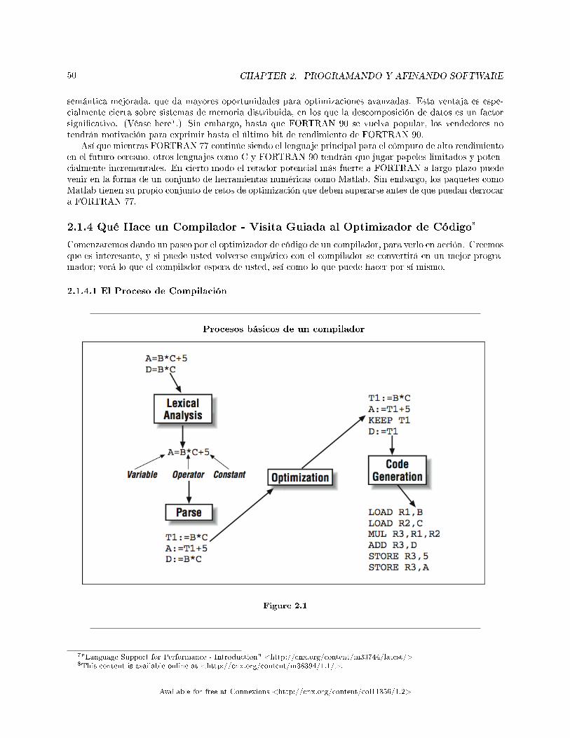
50 CHAPTER 2. PROGRAMANDO Y AFINANDO SOFTWARE
semántica mejorada, que da mayores oportunidades para optimizaciones avanzadas. Esta ventaja es espe-cialmente cierta sobre sistemas de memoria distribuida, en los que la descomposición de datos es un factorsigni�cativo. (Véase here7.) Sin embargo, hasta que FORTRAN 90 se vuelva popular, los vendedores notendrán motivación para exprimir hasta el último bit de rendimiento de FORTRAN 90.
Así que mientras FORTRAN 77 continúe siendo el lenguaje principal para el cómputo de alto rendimientoen el futuro cercano, otros lenguajes como C y FORTRAN 90 tendrán que jugar papeles limitados y poten-cialmente incrementales. En cierto modo el retador potencial más fuerte a FORTRAN a largo plazo puedevenir en la forma de un conjunto de herramientas numéricas como Matlab. Sin embargo, los paquetes comoMatlab tienen su propio conjunto de retos de optimización que deben superarse antes de que puedan derrocara FORTRAN 77.
2.1.4 Qué Hace un Compilador - Visita Guiada al Optimizador de Código8
Comenzaremos dando un paseo por el optimizador de código de un compilador, para verlo en acción. Creemosque es interesante, y si puede usted volverse empático con el compilador se convertirá en un mejor progra-mador; verá lo que el compilador espera de usted, así como lo que puede hacer por sí mismo.
2.1.4.1 El Proceso de Compilación
Procesos básicos de un compilador
Figure 2.1
7"Language Support for Performance - Introduction" <http://cnx.org/content/m33744/latest/>8This content is available online at <http://cnx.org/content/m38394/1.1/>.
Available for free at Connexions <http://cnx.org/content/col11356/1.2>
51
Típicamente, el proceso de compilación se divide en un número de pasos identi�cables, como se muestra enla Figure 2.1 (Procesos básicos de un compilador). Aunque no todos los compiladores estén implementadosexactamente de esta manera, ayuda a comprender las diferentes funciones que éstos deben realizar:
1. Una fase de precompilación o preprocesamiento, donde se realiza cierta manipulación textual sencilladel código fuente. El paso de preprocesamiento puede procesar o incluir archivos, así como realizarsubstituciones sencillas de cadenas de texto a lo largo del código.
2. La fase de análisis lexicográ�co es la que descompone las sentencias de código fuente entrantes entokens tales como variables, constantes, comentarios o elementos del lenguaje.
3. La fase de análisis sintáctico es la encargada de comprobar la sintaxis de la entrada, y el copiladortraduce el programa entrante a un lenguaje intermedio que está listo para su optimización.
4. Se le realizan una o más pasadas de optimización al lenguaje intermedio.5. Un generador de código objeto traduce el lenguaje intermedio a código ensamblador, tomando en
consideración los detalles arquitectónicos particulares del procesador en cuestión.
Conforme los compiladores se vuelven más y más so�sticados para poder dar hasta el último bit derendimiento del procesador, algunos de estos pasos (especialmente los de optimización y generación decódigo) se vuelven más y más confusos. En este capítulo nos enfocaremos en el optimizador de código tradi-cional de un compilador, y en los capítulos subsecuentes revisaremos más de cerca cómo hacen optimizacionesmás so�sticadas los compiladores modernos.
2.1.4.2 Representación en Lenguaje Intermedio
Como estamos más interesados en la optimización de nuestro programa, comenzaremos nuestra discusión apartir de la salida de la fase de análisis sintáctico del compilador. Dicha salida está en la forma de un lenguajeintermedio (LI), algo entre un lenguaje de alto nivel y un lenguaje ensamblador. El lenguaje intermedioexpresa los mismos cálculos que en el programa original, en una forma que el compilador pueda manipularmás fácilmente. Es más, ciertas instrucciones que no están presentes en el fuente, tales como expresiones dedireccionamiento para referencias a arreglos, se hacen visibles junto con el resto del programa, haciéndolotambién de este modo sujeto de optimización.
¾Cómo luce un lenguaje intermedio? En términos de complejidad, es similar a un código ensamblador,pero no tan simple como para que se pierdan las de�niciones9 y usos de las variables. Necesitaremos lainformación acerca de de�nición y uso para analizar el �ujo de datos a través del programa. Típicamentelos cálculos se expresan como u �ujo de cuádruplas � sentencias con exactamente un operador, (hasta) dosoperandos, y un resultado.10 Presuponiendo que cualquier cosa en el programa fuente original pueda cambiarsu representación en términos de cuádruplas, tenemos un lenguaje intermedio utilizable. Para darnos unaidea de cómo trabaja, reescribiremos la sentencia siguiente como una serie de cuatro cuádruplas:
A = -B + C * D / E
Tomando todo como una unidad, la sentencia tiene cuatro operadores y cuatro operandos: /, *, + y -
(negación), y B, C, D, y E. Claramente es demasiado para que quepa en una cuádrupla. Necesitamos unaforma con exactamente un operador y, cuando mucho, dos operandos por sentencia. La versión que sigue lolleva a cabo, empleando variables temporales para almacenar los resultados intermedios:
T1 = D / E
T2 = C * T1
9Por "de�niciones" nos referimos a la asignación de valores, no a las declaraciones.10De manera más general, el código puede representarse como n-tuplas. Depende del nivel del lenguaje intermedio.
Available for free at Connexions <http://cnx.org/content/col11356/1.2>
52 CHAPTER 2. PROGRAMANDO Y AFINANDO SOFTWARE
T3 = -B
A = T3 + T2
Por supuesto, un lenguaje intermedio utilizable requiere de algunas otras características, como apuntadores.Estamos por sugerir la creación de nuestro propio lenguaje intermedio para investigar cómo trabajan lasoptimizaciones. Para comenzar, necesitamos establecer unas pocas reglas:
• Las instrucciones están formadas por un código de operación, dos operandos y un resultado. Dependi-endo de la instrucción, los operandos pueden quedar vacíos.
• Las asignaciones adoptan la forma X := Y op Z, que signi�ca X optiene el resultado de op aplicado aY y Z.
• Todas las referencias a memoria son cargas explícitas desde, o bien almacenamiento a, variables "tem-porales" tn.
• Los valores lógicos usados en las bifurcaciones se calculan separadamente del salto actual.• Los saltos van a direcciones absolutas.
Si estamos construyendo un compilador, deberemos ser un poco más especí�cos. Para nuestros propósitoscon esto basta. Considere el siguiente fragmento de código en C:
while (j < n) {
k = k + j * 2;
m = j * 2;
j++;
}
Este ciclo se traduce en la representación en lenguaje intermedio que se muestra a continuación:
A:: t1 := j
t2 := n
t3 := t1 < t2
jmp (B) t3
jmp (C) TRUE
B:: t4 := k
t5 := j
t6 := t5 * 2
t7 := t4 + t6
k := t7
t8 := j
t9 := t8 * 2
m := t9
t10 := j
t11 := t10 + 1
j := t11
jmp (A) TRUE
C::
Available for free at Connexions <http://cnx.org/content/col11356/1.2>
53
Cada línea de código fuente en C se representa mediante varias sentencias en LI. En muchos procesadoresRISC, nuestro código LI es tan parecido al lenguaje máquina que podemos traducirlo directamente a códigoobjeto.11 A menudo el nivel más bajo de optimización consiste en una traducción literal del lenguajeintermedio a código máquina. Cuando esto sucede, el código generalmente es muy largo y su rendimientoes pobre. Al revisarlo, puede usted encontrar lugares donde ahorrar unas pocas instrucciones. Por ejemplo,j se carga en variables temporales en cuatro lugares; seguramente podemos reducirlo. Tenemos que realizaralgo de análisis y algunas optimizaciones.
2.1.4.3 Bloques Básicos
Tras generar nuestro lenguaje intermedio, queremos cortarlo en bloques básicos. Se trata de secuencias decódigo que comienzan con una instrucción que o bien sigue una bifurcación o es en sí misma el destino deun salto. Dicho de otra forma, cada bloque básico tiene una entrada (en la parte superior) y una salida (enla parte inferior). Figure 2.2 (Lenguaje intermedio dividido en bloques básicos) representa nuestro códigoLI como un grupo de tres bloques básicos. Estos bloques hacen el código más fácil de analizar. Al restringirel �ujo de control al interior de un bloque básico de arriba hacia abajo y eliminar todas las bifurcaciones,podemos asegurarnos que si se ejecuta la primera sentencia, también lo hará la segunda, y así sucesivamente.Por supuesto, las bifurcaciones no han desaparecido, pero las hemos forzado afuera de los bloques en la formade �echas de conexión - el grafo de �ujo.
11Véase Section 5.2.1 para algunos ejemplos de código máquina obtenido directamente a partir de lenguaje intermedio.
Available for free at Connexions <http://cnx.org/content/col11356/1.2>
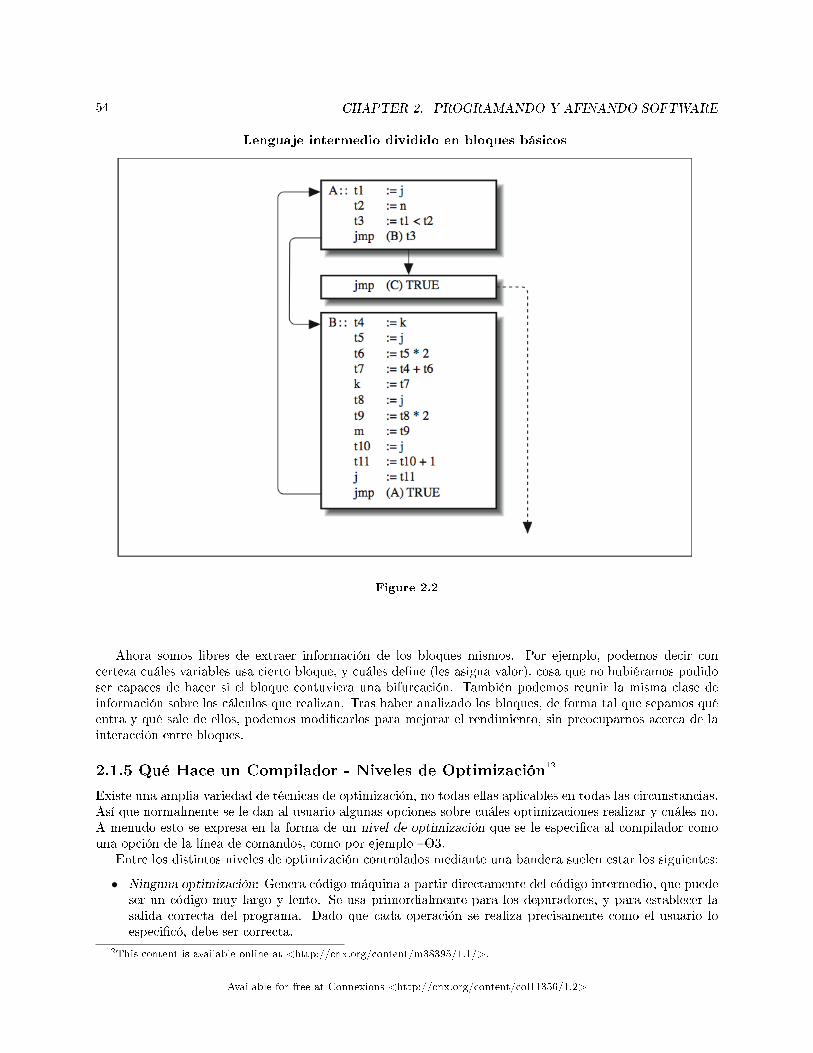
54 CHAPTER 2. PROGRAMANDO Y AFINANDO SOFTWARE
Lenguaje intermedio dividido en bloques básicos
Figure 2.2
Ahora somos libres de extraer información de los bloques mismos. Por ejemplo, podemos decir concerteza cuáles variables usa cierto bloque, y cuáles de�ne (les asigna valor), cosa que no hubiéramos podidoser capaces de hacer si el bloque contuviera una bifurcación. También podemos reunir la misma clase deinformación sobre los cálculos que realizan. Tras haber analizado los bloques, de forma tal que sepamos quéentra y qué sale de ellos, podemos modi�carlos para mejorar el rendimiento, sin preocuparnos acerca de lainteracción entre bloques.
2.1.5 Qué Hace un Compilador - Niveles de Optimización12
Existe una amplia variedad de técnicas de optimización, no todas ellas aplicables en todas las circunstancias.Así que normalmente se le dan al usuario algunas opciones sobre cuáles optimizaciones realizar y cuáles no.A menudo esto se expresa en la forma de un nivel de optimización que se le especi�ca al compilador comouna opción de la línea de comandos, como por ejemplo �O3.
Entre los distintos niveles de optimización controlados mediante una bandera suelen estar los siguientes:
• Ninguna optimización: Genera código máquina a partir directamente del código intermedio, que puedeser un código muy largo y lento. Se usa primordialmente para los depuradores, y para establecer lasalida correcta del programa. Dado que cada operación se realiza precisamente como el usuario loespeci�có, debe ser correcta.
12This content is available online at <http://cnx.org/content/m38395/1.1/>.
Available for free at Connexions <http://cnx.org/content/col11356/1.2>
55
• Optimizaciones básicas:Similares a las descritas en este capítulo. Generalmente trabaja minimizandoel lenguaje intermedio y generando código compacto y rápido.
• Análisis interprocedimental: Observa más allá de las fronteras de una única rutina, en busca de oportu-nidades de optimización. Este nivel de optimización puede incluir extender una optimización bñásica,tal como la propagación de copias, a través de múltiples rutinas. Otro resultado de esta técnica es lainserción de procedimientos en línea (inline) en aquellos lugares donde mejore el rendimiento.
• Análisis de per�l a tiempo de ejecución: Es posible usar el per�lado a tiempo de ejecución para ayudaral compilador a generar código mejorado, basado en su conocimiento de los patrones de ejecución atiempo de ejecución, reunidos a partir de la información del per�l.
• Optimizaciones de punto �otante: El estándar de punto �otante del IEEE (IEEE 754) especi�cacon precisión cómo se llevan a cabo las operaciones de punto �otante. El compilador puede identi�carciertas transformaciones algebraicas que incrementan la velocidad del programa (tales como reemplazaruna división con un recíproco una multiplicación), pero ello pudiera cambiar los resultados de salidarespecto al código no optimizado.
• Análisis de �ujo de datos: Identi�ca el paralelismo potencial entre instrucciones, bloques o inclusoiteraciones sucesivas de bucles.
• Optimización avanzada: Puede incluir vectorización, paralelización o descomposición de datos au-tomáticas en computadoras con arquitecturas avanzadas.
Tales optimizaciones pueden controlarse mediante varias opciones distintas del compilador. A menudo selleva algún tiempo cavilar la mejor combinación de banderas de compilación para un código o conjunto decódigos en particular. En algunos casos, los programadores compilan diferentes rutinas usando diferentescon�guraciones de optimización, para lograr el mejor rendimiento global.
2.1.6 Qué Hace un Compilador - Optimizaciones Clásicas13
Una vez dividido el lenguaje intermedio en bloques básicos, hay diversas optimizaciones que pueden realizarsesobre el código de tales bloques. Algunas son muy simples y afectan a unas pocas tuplas dentro de un bloquebásico. Otras mueven código de un bloque básico a otro, sin alterar los resultados del programa. Por ejemplo,a menudo resulta útil mover una cálculo desde el cuerpo de un ciclo al código que precede de forma inmediataal bucle.
En esta sección, vamos a listar por nombre las optimizaciones clásicas, e indicarle a usted para qué son.No estamos sugiriendo que usted haga los cambios; la mayoría de lso compiladores desde mitad de la décadade 1980 realizan de modo completamente automático tales optimizaciones, excepto en el nivel más bajo deoptimización. Como vimos a inicios del capítulo, si comprende usted aquello que pueden (y que no pueden)hacer los compiladores, se convertirá en un mejor programador porque será capaz de jugar con las fortalezasde ellos.
2.1.6.1 Propagación de Copia
Para iniciar, veamos una técnica para desenredar cálculos. Échele un vistazo al siguiente segmento de código:observe los dos cálculos que involucran a X.
X = Y
Z = 1.0 + X
Tal como está escrito, la segunda sentencia requiere del resultado de la primera antes de que pueda ejecutarse-requiere usted de X para calcular Z. Las dependencias innecesarias a menudo se traducen en retrasos a tiempo
13This content is available online at <http://cnx.org/content/m38400/1.1/>.
Available for free at Connexions <http://cnx.org/content/col11356/1.2>
56 CHAPTER 2. PROGRAMANDO Y AFINANDO SOFTWARE
de ejecución. 14 Realizando algunos reacomodos, podemos hacer que la segunda sentencia sea independientede la primera, al propagar una copia de Y. El nuevo cálculo para Z usa el valor de Y directamente:
X = Y
Z = 1.0 + Y
Observe que dejamos intacta la sentencia X=Y. Puede que usted se pregunte, "¾por qué dejarla así?" Elproblema es que no podemos decir en qué otras partes se requiere el valor de X. Eso es algo que deberádecidir otro análisis. Si resulta que ninguna otra sentencia requiere del valor de X, la asignación se eliminaráposteriormente, por medio de la remoción de código muerto.
2.1.6.2 Plegado de Constantes
Un compilador inteligente puede encontrar constantes a lo largo de su programa. Algunas de ellas son�obvias�, como aquellas de�nidas en las sentencias de parámetros. Otras resultan menos obvias, tales comolas variables locales que nunca se rede�nen. Cuando las combina en un cálculo, obtiene una expresiónconstante. El pequeño programa siguiente tiene dos constantes, I y K:
PROGRAM MAIN
INTEGER I,K
PARAMETER (I = 100)
K = 200
J = I + K
END
Dado que tanto I como K son constantes individualmente, la combinación de I+K es constante, lo cuál signi�caque J también es una constante. El compilador reduce las expresiones constantes como I+K a constantes,mediante una técnica llamada plegado de constantes.
¾Cómo funciona el plegado de constantes? Puede ver que es posible examinar cada camino en el cuálpuede de�nirse una variable en ruta hacia un bloque básico particular. Si descubre usted que todos loscaminos se inician en el mismo valor, éste es constante; puede reemplazar todas las referencias a esa variablecon una constante. Este reemplazo tiene un efecto de rizado a lo largo de la ruta. Si el compilador se percatade que encontró una expresión compuesta solamente por constantes, puede evaluarla a tiempo de compilacióny reemplazarla por una constante. Tras varias iteraciones, el compilador habrá localizado la mayoría de lasexpresiones que son candidatas al plegado de constantes.
A veces un programador puede mejorar el rendimiento, al hacer al compilador consciente de los valoresconstantes en su aplicación. Por ejemplo, en el siguiente segmento de código:
X = X * Y
el compilador generará código muy diferente a tiempo de ejecución si sabe que Y valía 0, 1, 2, or 175.32.Si no conoce el valor para Y, debe generar la secuencia de código más conservadora (no necesariamente lamás rápida). Un programador puede comunicarle esos valores a través del uso de la sentencia PARAMETER en
14Este código es un ejemplo de dependencia de �ujo. Describo las dependencias en detalle en(<http://cnx.org/content/m32775/latest/>).
Available for free at Connexions <http://cnx.org/content/col11356/1.2>
57
FORTRAN. Mediante el empleo de dicha sentencia, el compilador conoce los valores para estas constantesa tiempo de ejecución. Otro ejemplo que hemos visto es:
DO I = 1,10000
DO J=1,IDIM
.....
ENDDO
ENDDO
Tras revisar el código, es claro que IDIM era uno de los valores 1, 2, or 3, dependiendo del conjunto de datosen uso. Claramente si el compilador sabía que IDIM valía 1, puede generar un código mucho más simple yrápido.
2.1.6.3 Remoción de Código Muerto
A menudo los programas contienen secciones de código muerto que no tiene efecto en las respuestas, y quepor tanto puede quitarse. Ocasionalmente, quien escribe el código muerto en el programa es el autor, peroes más común que sea el propio compilador quien lo hace; muchas optimizaciones producen código muertoque hay que barrer después.
Hay dos tipos de código muerto:
• Instrucciones inalcanzables• Instrucciones que producen resultados que jamás se usan
Es fácil que usted escriba código inalcanzable en su programa, al hacer que el �ujo de control pase alrededorde él - permanentemente. Si el compilador puede decir que es inalcanzable, lo eliminará. Por ejemplo, esimposible alcanzar la sentencia I = 4 en este programa:
PROGRAM MAIN
I = 2
WRITE (*,*) I
STOP
I = 4
WRITE (*,*) I
END
El compilador desechará todo hasta la sentencia STOP, y probablemente le envíe un aviso. El código inalcan-zable producido por el compilador durante la optimización se retirará silenciosamente.
Los cálculos con variables locales pueden producir resultados que nunca se usan. Al analizar la de�nicióny usos de una variable, el compilador puede ver qué otras partes de la rutina la referencian. Por supuesto elcompilador no puede decir el destino último de las variables que se pasan entre rutinas, externas o comunes,así que tales cálculos siempre se mantienen (siempre y cuando sean alcanzables).15 En el siguiente programa,los cálculos que involucran a k no contribuyen en absoluto a la respuesta �nal, y son buenos candidatos parala eliminación de código muerto:
15Si un compilador realiza un análisis interprocedimental su�ciente, puede incluso optimizar variables entre fronteras derutinas. El análisis interprocedimental puede ser la perdición para los códigos de bancos de pruebas si trata de medir el tiempode un cálculo sin usar los resultados del mismo.
Available for free at Connexions <http://cnx.org/content/col11356/1.2>
58 CHAPTER 2. PROGRAMANDO Y AFINANDO SOFTWARE
main ()
{
int i,k;
i = k = 1;
i += 1;
k += 2;
printf ("%d\n",i);}
La eliminación de código muerto a menudo produce algunos resultados sorprendentes con bancos de pruebaspobremente escritos. Véase para un ejemplo de este tipo de código.
2.1.6.4 Reducción de Intensidad
Las operaciones o expresiones tienen costos de tiempo asociados. A veces es posible reemplazar un cálculomuy caro por otro más económico. Llamamos a esto reducción de intensidad. El siguiente fragmento decódigo contiene dos operaciones caras:
REAL X,Y
Y = X**2
J = K*2
En operaciones de exponenciación como la de la primera línea, el compilador generalmente incrusta unallamada a una rutina matemática de biblioteca. En dicha rutina, X se convierte a un logaritmo, se multiplicay luego se reconvierte. Sobre todo, elevar X a una potencia resulta caro -quizás tome cientos de ciclos demáquina. La clave es observar que X se está elevando a una potencia entera y pequeña. Una alternativa muchomás económica consiste en expresarlo como X*X, y pagar sólo el costo de una multiplicación. La segundasentencia muestra la multiplicación entera de una variable K por 2. Sumar K+K da el mismo resultado, perotoma menos tiempo.
Hay muchas oportunidades para reducción de intensidad generada por el compilador; éstas son sólodos de ellas. Veremos un caso especialmente importante cuando analicemos la simpli�cación de variablepor inducción. Otro ejemplo de una reducción de intensidad es reemplazar las multiplicaciones de enterospotencia de dos por desplazamientos lógicos.
2.1.6.5 Renombramiento de Variables
En Section 5.1.1, hablamos acerca de renombrar registros. Algunos procesadores pueden tomar decisionesa tiempo de ejecución para reemplazar todas las referencias al registro 1 por referencias al registro 2, porejemplo, para evitar cuellos de botella. El renombramiento de registros evita que las instrucciones que estánreciclando los mismos registros para propósitos diferentes, tengan que esperar hasta que las instruccionesprevias hayan dejado de usarlos.
La misma situación puede ocurrir en los programas - la misma variable (i.e. posición de memoria) puedereciclarse para dos propósitos no relacionados. Por ejemplo, observe la variable x en el siguiente fragmento:
Available for free at Connexions <http://cnx.org/content/col11356/1.2>
59
x = y * z;
q = r + x + x;
x = a + b;
Cuando el compilador reconoce que se está reciclando una variable, esto es que sus usos actual y futuros sonindependientes, puede sustituirla por una nueva variable para mantener los cálculos separados:
x0 = y * z;
q = r + x0 + x0;
x = a + b;
El renombramiento de variables es una técnica importante, porque deja en claro cuáles cálculos son inde-pendientes los unos de los otros, lo cuál mejora el número de cosas que pueden hacerse en paralelo.
2.1.6.6 Eliminación de Subexpresiones Comunes
Las subexpresiones son partes de expresiones más grandes. Por ejemplo, A+B es una subexpresión de C*(A+B).Si A+B aparece en varios lugares, como sucede a continuación, le llamamos una subexpresión común:
D = C * (A + B)
E = (A + B)/2.
En vez de calcular A + B dos veces, el compilador puede generar una variable temporal y usarla dondequieraque se necesite A + B:
temp = A + B
D = C * temp
E = temp/2.
Algunos compiladores se esfuerzan más que otros en encontrar subexpresiones comunes. Se reconocen lamayoría de los pares, tales como A+B. Algunos pueden reconocer la reutilización de intrínsecos, tales comoSIN(X). Pero no espere que el compilador vaya mucho más allá. Subexpresiones como A+B+C no son com-putacionalmente equivalentes a formas reasociadas como B+C+A, aunque sean algebraicamente equivalentes.Con el �n de proporcionar resultados predecibles en los cálculos, FORTRAN debe o bien realizar las opera-ciones en el orden especi�cado por el usuario, o bien reordenarlos en una forma que garantice exactamente elmismo resultado. A veces el usuario no se preocupa de la forma en que se asocia A+B+C, pero el compiladorno puede asumir que al usuario no le preocupa.
El cálculo de direcciones proporciona una oportunidad particularmente rica para la eliminación de subex-presiones comunes. Usted no requiere ver los cálculos en el código fuente, pues los genera el compilador.Por ejemplo, una referencia al elemento de un arreglo A(I,J) puede traducirse a una expresión en lenguajeintermedio tal como:
Available for free at Connexions <http://cnx.org/content/col11356/1.2>
60 CHAPTER 2. PROGRAMANDO Y AFINANDO SOFTWARE
address(A) + (I-1)*sizeof_datatype(A)
+ (J-1)*sizeof_datatype(A) * column_dimension(A)
Si A(I,J) se usa más de una vez, tenemos múltiples copias del mismo cálculo de direcciones. La eliminaciónde subexpresiones comunes descubrirá y agrupará (con un poco de suerte) los cálculos redundantes.
2.1.6.7 Remoción de Código Invariante en Bucles
Es en los bucles donde los programas de cómputo de alto rendimiento gastan la mayoría de su tiempo. Elcompilador busca cada oportunidad que tiene de mover cálculos fuera del cuerpo de un bucle hacia el códigoque lo rodea. Las expresiones que no cambian después de haber ingresado al ciclo (expresiones invariantesen el bucle) son la primera opción. El siguiente ciclo tiene dos expresiones invariantes:
DO I=1,N
A(I) = B(I) + C * D
E = G(K)
ENDDO
A continuación, hemos modi�cado las expresiones para mostrar cómo pueden moverse afuera del ciclo:
temp = C * D
DO I=1,N
A(I) = B(I) + temp
ENDDO
E = G(K)
Es posible mover el código antes o después del cuerpo del bucle. Como sucede con la eliminación de subex-presiones comunes, la aritmética de direcciones resulta un blanco particularmente importante para la técnicade movimiento de invariantes en los bucles. Las porciones que cambian lentamente en el cálculo de los índicespueden enviarse a los suburbios, para ejecutarse sólo cuando se requieran.
2.1.6.8 Simpli�cación de Variables de Inducción
Los ciclos pueden contener lo que se conoce como variables de inducción. Su valor cambia como una funciónlineal del contador de iteraciones del ciclo. Por ejemplo, K es una variable de inducción en el siguiente bucle.Su valor está ligado al índice del ciclo:
DO I=1,N
K = I*4 + M
Available for free at Connexions <http://cnx.org/content/col11356/1.2>
61
...
ENDDO
La simpli�cación de variables de inducción reemplaza los cálculos que involucran variables como K por otrasmás simples. Dado un punto de inicio y la primera derivada de la expresión, puede usted llegar al valor deK para la n-ésima iteración, recorriendo paso a paso las n-1 iteraciones que intervienen:
K = M
DO I=1,N
K = K + 4
...
ENDDO
Ambas formas del bucle no son equivalentes; la segunda no le proporciona a usted el valor de K, dado cualquiervalor de I. Dado que no podemos saltar en la mitad del bucle a la n-ésima iteración, K siempre toma losmismos valores que hubiera tenido si hubiéramos dejado la expresión original.
Las simpli�cación de variables de inducción probablemente no sea una optimización muy importante,excepto que el cálculo de direcciones de los arreglos se parece mucho al cálculo de K en el ejemplo anterior.Por ejemplo, el cálculo de direcciones para A(I) dentro de un bucle iterando sobre la variable I se ve más omenos así:
address = base_address(A) + (I-1) * sizeof_datatype(A)
Realizar toda esta matemática es innecesario. El compilador puede crear una nueva variable de inducciónpara las referencias a A y simpli�car el cálculo de direcciones:
afuera del ciclo...
address = base_address(A) - (1 * sizeof_datatype(A))
dentro del ciclo...
address = address + sizeof_datatype(A)
La simpli�cación de variables de inducción resulta especialmente útil en aquellos procesadores que puedenincrementar automáticamente un registro cada vez que se utiliza un apuntador para una referencia a memoria.Mientras se recorre el ciclo paso a paso, tanto la referencia a memoria como la aritmética de direccionespueden exprimirse en una sola instrucción -un gran ahorro.
2.1.6.9 Generación de Código Objeto
La precompilación, los análisis lexicográ�co y sintáctico y muchas técnicas de optimización son a menudotransportables, pero la generación de código es muy especí�ca del procesador destino. En cierta forma es enesta fase donde los compiladores desquitan su precio, en los sistemas RISC de un solo procesador.
Cualquier cosa que no se haga en hardware debe realizarse en software. Ello signi�ca que si el procesadorno puede resolver con�ictos de recursos, tales como la sobreutilización de un registro o �la de procesamiento, elcompilador deberá hacerse cargo del asunto. Permitir que el compilador se ocupe de ello no es necesariamente
Available for free at Connexions <http://cnx.org/content/col11356/1.2>
62 CHAPTER 2. PROGRAMANDO Y AFINANDO SOFTWARE
malo, más bien es una decisión de diseño. Un compilador complicado y un hardware simple y rápido puedentener una alta relación costo/bene�cio para ciertas aplicaciones. Dos procesadores que se encuentran enlos extremos de este espectro son el MIPS R2000 y el HP PA-8000. El primero depende fuertemente delcompilador para plani�car las instrucciones y distribuir los recursos equitativamente. El segundo administraambas cosas a tiempo de ejecución, aunque ambos dependan del compilador para proporcionar una mezclade instrucciones equitativa.
En todas las computadoras, la selección de registros es un reto porque, dependiendo de su número, losregistros son recursos preciosos. Usted quiere asegurarse que las variables más activas residan permanente-mente en los registros, a expensas de otras. En aquellas máquinas sin renombramiento de registros (véaseSection 5.1.1), usted debe asegurarse que el compilador no trate de reciclar los registros demasiado rápido,o de otra forma el procesador tendrá que retrasar los cálculos, en espera de que alguno de ellos se libere.
Algunas instrucciones del repertorio también hacen que su compilador no tenga que ejecutar otras.Ejemplo de esto son el autoincremento de los registros que se usan como índices de arreglos, o el uso deasignaciones condicionales en vez de bifurcaciones. Ambas ahorran al procesador realizar cálculos extras,produciendo un �ujo de instrucciones más compacto.
Finalmente, están las oportunidades para incrementar el paralelismo. Los programadores generalmentepiensan serialmente, especi�cando pasos en sucesión lógica. Desafortunadamente, el código fuente serialproduce código objeto serial. Un compilador que aspire a usar e�cientemente el paralelismo del procesador,deberá ser capaz de mover instrucciones y encontrar operaciones que puedan realizarse simultáneamente.Este es uno de los mayores retos de los creadores de compiladores actualmente. Conforme los diseñossuperescalares y de tamaño de instrucción muy grande (VLIW, Very Long Instruction Word) se vuelvencapaces de ejecutar más instrucciones por ciclo de reloj, el compilador tendrá que excavar más profundamenteen busca de operaciones que puedan ejecutarse a la vez.
2.1.7 Qué Hace un Compilador - Notas de Cierre16
Este capítulo ha sido una introducción básica a la forma en que funciona el optimizador de código de uncompilador. Sin embargo, no es lo último que diremos acerca de los compiladores. Con el objeto de realizar lavectorización, paralelización y descomposición de datos automáticamente, los compiladores adicionalmentedeben analizar el código fuente. Conforme nos topemos con estos tópicos, iremos discutiendo el impactosobre y del compilador, y cómo los programadores pueden interactuar mejor con éste.
En las arquitecturas RISC modernas de un solo procesador, los compiladores por lo general producenmejor código que la mayoría de los programadores humanos en ensamblador. En vez de tratar de compensarel trabajo de un compilador simplista agregando optimizaciones a mano, nosotros como programadoresdebemos mantener nuestros programas simples, de forma que no confundan a éste. Al entender los patronesque los compiladores son capaces de optimizar, podemos enfocarnos en escribir programas sencillos que seantransportables y comprensibles.
2.1.8 Qué Hace un Compilador - Ejercicios17
Exercise 2.1.8.1¾Su compilador reconoce el código muerto en el siguiente programa? ¾Cómo puede estar seguro?¾Le envía el compilador algún aviso?
main()
{
int k=1;
16This content is available online at <http://cnx.org/content/m38402/1.1/>.17This content is available online at <http://cnx.org/content/m38401/1.1/>.
Available for free at Connexions <http://cnx.org/content/col11356/1.2>

63
if (k == 0)
printf ("Esta sentencia nunca se ejecuta.\n");}
Exercise 2.1.8.2Compile el siguiente código, y ejecútelo bajo distintos niveles de optimización.
Trate de adivinar los distintos tipos de optimizaciones que se están realizando para mejorar elrendimiento, conforme se incrementa el nivel de optimización.
REAL*8 A(1000000)
DO I=1,1000000
A(I) = 3.1415927
ENDDO
DO I=1,1000000
A(I) = A(I) * SIN(A(I)) + COS(A(I)) ENDDO
PRINT *,"Terminado"
Exercise 2.1.8.3Tome el siguiente segmento de código y compílelo a varios niveles de optimización. Observe elcódigo ensamblador generado (en algunos compiladores esto se hace con la opción -S) y encuentrelos efectos de cada nivel de optimización sobre el lenguaje máquina. Mida el tiempo de ejecución delprograma para ver el rendimiento a diferentes niveles de optimización. Si tiene acceso a múltiplesarquitecturas, observe el código generado usando los mismos niveles de optimización sobre diferentesarquitecturas.
REAL*8 A(1000000)
COMMON/BLK/A
.... Llamada para medir el tiempo
DO I=1,1000000
A(I) = A(I) + 1.234
ENDDO
.... Llamada para medir el tiempo
END
¾Por qué es necesario poner el arreglo adentro de un bloque común?
2.2 Cronometraje y Per�lado
2.2.1 Cronometraje y Per�lado - Introducción18
Tal vez con hacer que su código produzca las respuestas correctas sea su�ciente. Después de todo, si sóloplanea usar el programa de vez en cuando, o si sólo toma unos minutos en ejecutarse, el tiempo de ejecución
18This content is available online at <http://cnx.org/content/m38404/1.2/>.
Available for free at Connexions <http://cnx.org/content/col11356/1.2>

64 CHAPTER 2. PROGRAMANDO Y AFINANDO SOFTWARE
no es un asunto que le importe demasiado. Pero puede que no siempre ese sea el caso. Típicamente, la gentese preocupa por el tiempo de ejecución de sus programas por una de dos razones:
• La carga de trabajo ha crecido.• Están considerando una nueva máquina.
Resulta claro por qué debe usted preocuparse acerca del rendimiento de su programa si la carga de trabajocrece. Tratar de atiborrar 25 horas de tiempo de cómputo en un día de 24 horas es una pesadilla adminis-trativa. Pero, ¾por qué debiera preocuparse la gente que está considerando una nueva máquina, acerca deltiempo de ejecución? Después de todo, la nueva máquina presumiblemente será más rápida que la antigua,así que todo debiera tomar menos tiempo. La razón es que cuando la gente está evaluando nuevas máquinas,requieren una base de comparación -un banco de pruebas. La gente a menudo usa programas que le resultanfamiliares como banco de pruebas. Tiene sentido: usted quiere un banco de prueba que sea representativode la clase de trabajos que realiza, y nada es más representativo del trabajo que usted hace... ½que el trabajoque usted hace!
Llevar a cabo bancos de pruebas suena fácil, suponiendo que tenga usted herramientas de cronometraje.19 Usted sólo quiere asegurarse que lo que tales herramientas estén reportando sea lo mismo que usted piensaque está obteniendo; especialmente si nunca las ha utilizado con anterioridad. Para ilustrar el punto, imaginesi alguien tomase su reloj y lo reemplazara con otro que expresa el tiempo en un sistema de unidades exótico, ocon tres conjuntos de manecillas sobrepuestas. Resultaría muy confuso; tendría problemas leyéndolo. Estaríajusti�cablemente nervioso de tener que conducir sus asuntos mediante un reloj que no comprende.
Las herramientas de cronometraje de UNIX son como el reloj de seis agujas, reportando tres tiposdiferentes de medidas. No proporcionan información incongruente, sólo presentan más información de la quepuede usted expresar mediante un único valor numérico. Nuevamente, el truco consiste en aprender a leereste reloj. Y eso es lo que hace la primera parte de este capítulo. Investigaremos los diferentes tipos demedidas que determinan el desempeño de un programa.
Si está usted planeando a�nar un programa, requiere más que sólo información de cronometraje. ¾Endónde se está gastando el tiempo, en un solo bucle, en una sobrecarga de llamado a subrutinas, o conproblemas de memoria? Para los a�nadores, las últimas secciones de este capítulo discutirán cómo per�larel código a nivel procedimental y de sentencia. También discutiremos qué signi�can los per�ladores, y cómopredicen el enfoque que debe usted tomar si decide meterle mano al código en busca de mayor rendimiento,y qué posibilidades tendrá de obtener éxito.
2.2.2 Cronometraje y Per�lado - Cronometraje20
Vamos a asumir que su programa se ejecuta correctamente. Resulta algo ridículo cronometrar un programaque no se está ejecutando bien, lo cual no quiere decir que no suceda. Dependiendo de lo que esté ustedhaciendo, puede estar interesado en saber cuánto tiempo gasta globalmente, o interesado sólo en una porcióndel programa. Le mostraremos cómo cronometrar primero el programa completo, y luego hablaremos acercade cronometrar bucles o subrutinas individuales.
2.2.2.1 Cronometrando un Programa Completo
En UNIX, puede usted cronometrar la ejecución de un programa poniendo el comando time antes quecualquier otro que normalmente teclee en la línea de comandos. Cuando el programa termina, se produceun sumario de cronometraje. Por ejemplo, si su programa se llama foo, puede cronometrar su ejecucióntecleando time foo. Si está usted usando el shell C o el shell Korn, time es uno de los comandos internos delshell. Con el shell Bourne, time es un comando separado, ejecutado desde /bin. En cualquier caso, aparecela siguiente información al �nal de la ejecución:
• Tiempo en modo usuario
19El tiempo es dinero.20This content is available online at <http://cnx.org/content/m38409/1.2/>.
Available for free at Connexions <http://cnx.org/content/col11356/1.2>

65
• Tiempo en modo sistema• Tiempo transcurrido
Estas �guras de cronometraje resultan más fáciles de entender con algo de conocimiento previo. Conformesu programa se ejecuta, conmuta de ida y vuelta entre dos modos fundamentalmente diferentes: el modo deusuario y el modo de kernel. El estado de operación normal es el modo de usuario, en el cual se ejecutan lasinstrucciones que el compilador generó por usted, además de cualquier llamada a una subrutina de bibliotecaenlazada con su programa. 21 Pudiera ser su�ciente con la ejecución en modo de usuario siempre, exceptoque los programas generalmente requieren otros servicios, tales como entrada/salida (I/O), y ello requierela intervención del sistema operativo -el núcleo o kernel. Una solicitud de servicio del kernel hecha por suprograma, o tal vez un evento externo al programa, causa la conmutación del modo de usuario al modo dekernel.
El tiempo empleado en la ejecución de cada uno de los dos modos se contabiliza por separado. Lamétrica del tiempo de usuario describe el tiempo gastado en el modo de usuario. Similarmente, la métricade tiempo de sistema indica el tiempo gastado en modo de kernel. Conforme avanza el tiempo de usuario,cada programa en la máquina se contabiliza por separado. Esto es, no le contabilizarán a usted la actividadrealizada por las aplicaciones de alguien más. El registro del tiempo de sistema funciona casi de la mismaforma; sin embargo, bajo ciertas circunstancias, puede ser que le contabilicen a usted algunos servicios desistema realizados a nombre de otras personas, además del suyo propio. Esta contabilidad incorrecta ocurreporque el programa de usted puede estar en ejecución al momento que alguna actividad externa causa unainterrupción. No parece justo, pero consuélese con el hecho de que esto funciona así en ambos sentidos:puede que a los otros usuarios también les contabilicen la actividad de sistema de usted, por la misma razón.
Juntos, los tiempos de usuario y de sistema se conocen como tiempo de CPU. Generalmente, el tiempode usuario es por mucho mayor que el tiempo de sistema. Esto es algo que cabe esperar, porque la mayoríade las aplicaciones sólo piden los servicios del sistema ocasionalmente. De hecho, un tiempo de sistemadesproporcionadamente grande probablemente indique algún problema. Por ejemplo, aquellos programasque generan condiciones de excepción repetidamente, tales como fallos de página, referencias a memoriadesalineadas, o excepciones de punto �otante, usan una cantidad de tiempo de sistema poco usual. Eltiempo gastado en hacer cosas tales como buscar en disco, rebobinar una cinta, o esperar por caracteresprovenientes de la terminal no se contabilizan en el tiempo de CPU. Ello se debe a que tales actividades norequieren de la CPU, que está disponible para suspenderlo y ejecutar otros programas.
La tercera pieza de información (correspondiente al tercer conjunto de manecillas del reloj) el tiempotranscurrido, es una medida del tiempo actual (tiempo de reloj de pared) que ha pasado desde que el programainició. Para aquellos programas que gastan la mayoría de su tiempo calculando, el tiempo transcurrido debeser muy parecido al tiempo de CPU. Las razones por las cuales el tiempo transcurrido puede ser mayor son:
• Está usted compartiendo el tiempo de máquina con otros programas.22
• Su aplicación lleva a cabo mucha I/O• Su aplicación requiere más ancho de banda de memoria que la que está disponible en la máquina.• Su programa está llevando a cabo paginación o intercambio.
La gente a menudo registra el tiempo de CPU y lo usa como un estimado del tiempo transcurrido. Usarel tiempo de CPU está bien cuando se trata de máquinas de una sola CPU, suponiendo que ha visto ustedejecutarse el programa cuando la máquina estaba tranquila y observó que ambos números eran muy parecidos.Pero para los multiprocesadores, el tiempo total de CPU puede ser muy diferente del tiempo transcurrido.Cada vez que haya dudas, espere hasta que tenga la máquina sólo para usted, y entonces cronometre suprograma, usando el tiempo transcurrido. Es muy importante producir resultados de cronometría quepuedan veri�carse usando otra corrida, cuando se estén usando los resultados para tomar decisiones decompra importantes.
21El tiempo de falla de caché también se consume aquí.22El comando uptime le proporciona una indicación aproximada del resto de la actividad en su máquina. Los últimos tres
campos le indican el número promedio de procesos listos para ejecutarse durante los últimos 1, 5 y 15 minutos respectivamente
Available for free at Connexions <http://cnx.org/content/col11356/1.2>
66 CHAPTER 2. PROGRAMANDO Y AFINANDO SOFTWARE
Si está ejecutando un UNIX derivado de Berkeley, el comando de cronómetro interno del shell C puedereportar otras estadísticas útiles. La forma por defecto de la salida que arroja se muestra en Figure 2.3 (Lafunción interna time de csh). Revise la página del manual de su csh para ver más posibilidades.
Además de los datos de tiempos de CPU y utilizado, el comando time de csh produce información acercadel uso de la CPU, fallos de página, intercambios, operaciones de E/S bloqueadas (usualmente actividad dedisco) y algunas medidas sobre cuánta memoria ocupaba nuestro programa cuando estaba en ejecución. Lasdescribiremos una a la vez.
2.2.2.1.1 Porcentaje de Uso
El porcentaje de uso corresponde a la tasa de tiempo usado respecto al tiempo de CPU. Como mencionamoscon anterioridad, existen varias razones por las que el uso de la CPU no sea del 100% o siquiera cercano. Amenudo puede usted obtener un indicio, a partir de los otros campos, de cuál es el problema con su programao si éste estaba compartiendo la máquina cuando lo ejecutaba.
2.2.2.1.2 Uso Promedio de Memoria Real
Las dos medidas de uso promedio de la memoria mostradas en Figure 2.3 (La función interna time de csh)caracterizan los requerimientos de recursos del programa conforme se ejecuta.
La primera medida, el espacio de memoria compartida, contabiliza la cantidad promedio de memoria realque ocupa el segmento de texto de su programa - la porción que almacena las instrucciones de máquina.Se le lama "compartida" porque pueden compartirlo varias copias del programa que estén actualmente enejecución (para ahorrar memoria). Años atrás, era posible que el segmento de texto consumiera una partesigni�cativa del sistema de memoria, pero en estos días, con tamaños de memoria a partir de los 32 MB,tiene usted que compilar un programa fuente realmente enorme y usar cada bit de él para que la cantidadque �gure en el uso de memoria compartida sea su�cientemente grande como para causar preocupación. Elrequerimiento de espacio de memoria compartida es usualmente muy bajo, en comparación a la cantidad dememoria disponible en su máquina.
Available for free at Connexions <http://cnx.org/content/col11356/1.2>
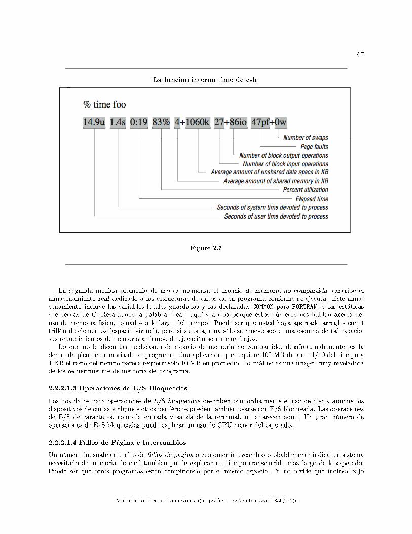
67
La función interna time de csh
Figure 2.3
La segunda medida promedio de uso de memoria, el espacio de memoria no compartida, describe elalmacenamiento real dedicado a las estructuras de datos de su programa conforme se ejecuta. Este alma-cenamiento incluye las variables locales guardadas y las declaradas COMMON para FORTRAN, y las estáticasy externas de C. Resaltamos la palabra "real" aquí y arriba porque estos números nos hablan acerca deluso de memoria física, tomados a lo largo del tiempo. Puede ser que usted haya apartado arreglos con 1trillón de elementos (espacio virtual), pero si su programa sólo se mueve sobre una esquina de tal espacio,sus requerimientos de memoria a tiempo de ejecución serán muy bajos.
Lo que no le dicen las mediciones de espacio de memoria no compartido, desafortunadamente, es lademanda pico de memoria de su programa. Una aplicación que requiere 100 MB durante 1/10 del tiempo y1 KB el resto del tiempo parece requerir sólo 10 MB en promedio - lo cuál no es una imagen muy reveladorade los requerimientos de memoria del programa.
2.2.2.1.3 Operaciones de E/S Bloqueadas
Los dos datos para operaciones de E/S bloqueadas describen primordialmente el uso de disco, aunque losdispositivos de cintas y algunos otros periféricos pueden también usarse con E/S bloqueada. Las operacionesde E/S de caracteres, como la entrada y salida de la terminal, no aparecen aquí. Un gran número deoperaciones de E/S bloqueadas puede explicar un uso de CPU menor del esperado.
2.2.2.1.4 Fallos de Página e Intercambios
Un número inusualmente alto de fallos de página o cualquier intercambio probablemente indica un sistemanecesitado de memoria, lo cuál también puede explicar un tiempo transcurrido más largo de lo esperado.Puede ser que otros programas estén compitiendo por el mismo espacio. Y no olvide que incluso bajo
Available for free at Connexions <http://cnx.org/content/col11356/1.2>
68 CHAPTER 2. PROGRAMANDO Y AFINANDO SOFTWARE
condiciones óptimas, cada programa sufre de cierto número de fallos de página, como se explicó en here23.En here24 se describen algunas técnicas para minimizar el número de fallos de página.
2.2.2.2 Cronometrando una Porción del Programa
Para algunos bancos de pruebas o esfuerzos de a�nación, las medidas tomadas desde "afuera" del programa leindican a usted todo lo que necesita saber. Pero si está tratando de aislar las cifras de rendimiento de bucleso porciones de código individuales, puede que quiera incluir rutinas de cronometraje también al interior. Latécnica básica es su�cientemente sencilla:
1. Registrar el tiempo antes de comenzar a hacer X.2. Hacer X.3. Registrar el tiempo al completar X.4. Restar el tiempo inicial del tiempo �nal.
Si, por ejemplo, el trabajo primario de X es calcular la posición de unas partículas, divida el tiempo total paraobtener un número de posiciones de partículas por segundo. Pero debe ser cuidadoso: si realiza demasiadosllamados a las rutinas de cronometraje, el observador se vuelve parte del experimento. Las rutinas decronometraje también consumen tiempo, y su sola presencia puede incrementar el número de fallos de cachede instrucciones o la paginación. Por otra parte, usted quiere que X tome una cantidad su�ciente de tiempoen ejecutarse, como para que las mediciones sean útiles. Es muy importante poner atención al tiempo entrellamadas al cronómetro, porque el reloj usado por las funciones cronométricas tiene una resolución limitada.Un evento que ocurra dentro de una fracción de segundo es difícil de medir con precisión.
2.2.2.3 Obteniendo Información de Tiempos
En esta sección, discutiremos métodos para obtener varios valores de cronometraje durante la ejecución desu programa.
Para los programas FORTRAN, una biblioteca de funciones de cronometraje disponible en muchasmáquinas se llama etime, que toma como argumento un arreglo de dos elementos REAL*4, y llena las celdascon el tiempo de CPU de usuario y el tiempo de CPU de sistema, respectivamente. El valor retornado porla función es la suma de los dos. He aquí un ejemplo de cómo se usa etime habitualmente:
real*4 tarray(2), etime
real*4 start, finish
start = etime(tarray)
finish = etime(tarray)
write (*,*) 'Tiempo de CPU: ', finish - start
No todos los vendedores proporcionan una función etime; de hecho, algunos no proporcionan rutinas decronometraje para FORTRAN en absoluto. Pruébelo primero. Si obtiene un mensaje de símbolo inde�nidocuando se enlace el programa, puede usar la siguiente rutina en C, que le proporciona la misma funcionalidadque etime:
23"Memory - Introduction" <http://cnx.org/content/m32733/latest/>24"Loop Optimizations - Introduction" <http://cnx.org/content/m33728/latest/>
Available for free at Connexions <http://cnx.org/content/col11356/1.2>
69
#include <sys/times.h>#define TICKS 100.
float etime (parts)
struct {
float user;
float system;
} *parts;
{
struct tms local;
times (&local);
parts->user= (float) local.tms_utime/TICKS;
parts->system = (float) local.tms_stime/TICKS;
return (parts->user + parts->system);
}
Hay un par de cosas que debe usted ajustar para hacerlo funcionar. Lo primero, para poder enlazar rutinasen C con rutinas en FORTRAN en su computadora, puede ser que deba agregar un guión bajo (_) tras elnombre de la función. Esto cambia la entrada a float etime_ (parts). Además, puede que deba ajustar elparámetro TICKS. Asumimos que el reloj del sistema tenía una resolución de 1/100 de segundo (cierto en lasmáquinas Hewlett-Packard para las que se escribió esta versión de etime). 1/60 es muy común. En una RS-6000 el número debiera ser 1000. Puede encontrar el valor en un archivo llamado /usr/include/sys/param.hen su máquina, o bien determinarlo empíricamente.
Abajo se muestra una rutina en C para recuperar la hora real, llamada gettimeofday. Está disponiblepara su uso ya sea en programas C o FORTRAN, y usa paso de parámetros por valor:
#include <stdio.h>#include <stdlib.h>#include <sys/time.h>
void hpcwall(double *retval)
{
static long zsec = 0;
static long zusec = 0;
double esec;
struct timeval tp;
struct timezone tzp;
gettimeofday(&tp, &tzp);
if ( zsec == 0 ) zsec = tp.tv_sec;
if ( zusec == 0 ) zusec = tp.tv_usec;
*retval = (tp.tv_sec - zsec) + (tp.tv_usec - zusec ) * 0.000001 ;
}
Available for free at Connexions <http://cnx.org/content/col11356/1.2>
70 CHAPTER 2. PROGRAMANDO Y AFINANDO SOFTWARE
void hpcwall_(double *retval) { hpcwall(retval); } /* Otra convención */
Dado que a menudo necesitará usted tanto el tiempo de CPU como la hora real, y que continuamente estarácalculando la diferencia entre sucesivas llamadas a tales rutinas, puede que quiera escribir una rutina queretorne el tiempo de reloj real y el tiempo de CPU cada vez que sea llamada, como sigue:
SUBROUTINE HPCTIM(WTIME,CTIME)
IMPLICIT NONE
*
REAL WTIME,CTIME
COMMON/HPCTIMC/CBEGIN,WBEGIN
REAL*8 CBEGIN,CEND,WBEGIN,WEND
REAL ETIME,CSCRATCH(2)
*
CALL HPCWALL(WEND)
CEND=ETIME(CSCRATCH)
*
WTIME = WEND - WBEGIN
CTIME = CEND - CBEGIN
*
WBEGIN = WEND
CBEGIN = CEND
END
2.2.2.4 Utilizando la Información de Cronometraje
Puede usted obtener mucha información de las facilidades de cronometraje que le proporciona una máquinaUNIX. No sólo puede decir cuánto tiempo lleva realizar cierto trabajo, sino también obtener indicios que ledigan si la máquina está operando e�cientemente, o si hay algún problema que requiera ser solucionado, talcomo una memoria inadecuada.
Una vez que el programa está ejecutándose con todas las anomalías antes explicadas, puede usted registrarel tiempo como una línea base. Si está a�nándolo, tal línea base será una referencia con la cuál podrá usteda�rmar si el proceso de a�nación ha mejorado mucho (o poco) las cosas. Si está realizando un banco depruebas, puede usar dicha línea base para juzgar cuánto incremento global de rendimiento le está dando unamáquina nueva. Pero recuerde observar también las otras cifras - paginación, uso de CPU, etc. ya que puedendiferir de máquina en máquina por razones que no están correlacionadas llanamente con el rendimiento dela CPU. Usted quiere asegurarse de obtener la imagen global.
2.2.3 Cronometraje y Per�lado - Per�lado de Subrutinas25
A veces va a desear más detalle que el que proporciona el cronometraje global de la aplicación, pero tal vezno tenga tiempo de modi�car el código para insertar varios cientos de llamadas a etime en su código. Losper�les también son muy útiles cuando le han entregado un extraño programa de 20,000 líneas de código, yle han pedido que averigue cómo funciona y luego mejore su rendimiento.
La mayoría de los compiladores proporcionan la facilidad de insertar llamadas cronométricas automáticasen su código, tanto a la entrada como a la salida de cada rutina, a tiempo de compilación. Cuando se
25This content is available online at <http://cnx.org/content/m38416/1.2/>.
Available for free at Connexions <http://cnx.org/content/col11356/1.2>
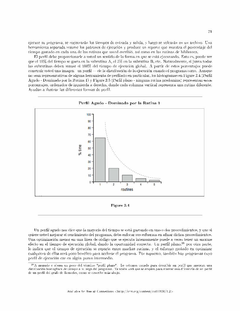
71
ejecute su programa, se registrarán los tiempos de entrada y salida, y luego se volcarán en un archivo. Unaherramienta separada resume los patrones de ejecución y produce un reporte que muestra el porcentaje deltiempo gastado en cada una de las rutinas que usted escribió, así como en las rutinas de biblioteca.
El per�l debe proporcionarle a usted un sentido de la forma en que se está ejecutando. Esto es, puede verque el 10% del tiempo se gasta en la subrutina A, el 5% en la subrutina B, etc. Naturalmente, si junta todaslas subrutinas deben sumar el 100% del tiempo de ejecución global. A partir de estos porcentajes puedeconstruir usted una imagen - un per�l � de la distribución de la ejecución cuando el programa corre. Aunqueno sean representativos de alguna herramienta de per�lado en particular, los histogramas en Figure 2.4 (Per�lAgudo - Dominado por la Rutina 1) y Figure 2.5 (Per�l plano - ninguna rutina predomina) representan estosporcentajes, ordenados de izquierda a derecha, donde cada columna vertical representa una rutina diferente.Ayudan a ilustrar las diferentes formas de per�l.
Per�l Agudo - Dominado por la Rutina 1
Figure 2.4
Un per�l agudo nos dice que la mayoría del tiempo se está gastando en uno o dos procedimientos, y que siquiere usted mejorar el rendimiento del programa, debe enfocar sus esfuerzos en a�nar dichos procedimientos.Una optimización menor en una línea de código que se ejecuta intensamente puede a veces tener un enormeefecto en el tiempo de ejecución global, dando la oportunidad correcta. Un per�l plano,26 por otra parte,le indica que el tiempo de ejecución se reparte entre muchas rutinas, y el esfuerzo gastado en optimizarcualquiera de ellas será poco bené�co para acelerar el programa. Por supuesto, también hay programas cuyoper�l de ejecución cae en algún punto intermedio.
26A menudo e abusa un poco del término "per�l plano". Lo estamos usando para describir un per�l que muestra unadistribución homogénea de tiempo a lo largo del programa. También verá que se emplea para marcar una diferencia de un per�lde un per�l del grafo de llamadas, como se describe más abajo.
Available for free at Connexions <http://cnx.org/content/col11356/1.2>

72 CHAPTER 2. PROGRAMANDO Y AFINANDO SOFTWARE
Per�l plano - ninguna rutina predomina
Figure 2.5
No podemos predecir con absoluta certeza qué será lo que encuentre usted cuando per�le sus programas,pero hay algunas tendencias generales. Por ejemplo, los códigos cientí�cos e ingenieriles construidos alrededorde soluciones matriciales a menudo exhiben per�les muy agudos. El tiempo de ejecución está dominado porel trabajo realizado en un puñado de rutinas. Para a�nar el código, necesita enfocar sus esfuerzos entales rutinas, hasta hacerlas más e�cientes. Puede que ello involucre reestructurar ciclos para exponer elparalelismo, proporcionar indicios al compilador, o reacomodar las referencias a memoria. En cualquier caso,el reto es tangible; puede ver los problemas que debe solucionar.
Por supuesto, existen límites a la mejora en tiempo de ejecución que obtendrá a�nando una o dosrutinas. Una regla de oro citada frecuentemente es la Ley de Amdahl, obtenida a partir de las observacionesrealizadas en 1967 por uno de los diseñadores de la serie 360 de IBM y fundador de Amdahl Computer,Gene Amdahl. Estrictamente hablando, sus observaciones fueron acerca del potencial de rendimiento de lascomputadoras paralelas, pero la gente ha adaptado la Ley de Amdahl para describir otras cosas por igual.Para nuestros propósitos, se puede citar así: digamos que tiene un programa con dos partes, una que puedeoptimizarse hasta hacerla in�nitamente rápida, y otra que no puede optimizarse en absoluto. Incluso si laporción optimizable supone como mucho el 50% del tiempo de ejecución inicial, cuando mucho será ustedcapaz de recortar el tiempo de ejecución total a la mitad. Esto es, su tiempo de ejecución estará dominadoeventualmente por la porción que no puede optimizarse. Esto pone un límite máximo a sus expectativas dea�nación.
Incluso a pesar del limitado retorno de inversión que sugiere la Ley de Amdahl, a�nar un programa con unper�l agudo puede dar sus recompensas. Los programas con per�les planos son mucho más difíciles de a�nar.A menudo se trata de códigos de sistema, aplicaciones no numéricas y variedades de códigos numéricos sinsoluciones matriciales. Se requiere de un enfoque de a�nación global para reducir, a un nivel justi�cable,el tiempo de ejecución de un programa con un per�l plano. Por ejemplo, a veces puede usted optimizar el
Available for free at Connexions <http://cnx.org/content/col11356/1.2>
73
uso de la cache de instrucciones, lo cuál resulta complicado por la distribución equitativa de actividades delprograma entre un gran número de rutinas. También puede ayudar a reducir la sobrecarga del llamado asubrutinas, plegando los invocados dentro de los invocadores. Ocasionalmente, puede encontrar un problemade referencia a memoria que es endémico al programa completo - y uno que puede arreglarse de un sologolpe.
Cuando estudie un per�l, puede que encuentre un porcentaje inusualmente grande de tiempo gastado enrutinas de biblioteca, tales como log, exp o sin. A menudo tales funciones se están realizando en rutinasde software, en vez de en línea. Puede reescribir su código para eliminar algunas de estas operaciones. Otropatrón importante que debe buscarse es aquel en el cual una rutina consume mucho más tiempo del queusted espera. Un tiempo de ejecución inesperado puede indicar que está accediendo a la memoria en unpatrón que resulta malo desde el punto de vista del rendimiento, o que algún aspecto del código no puedeoptimizarse apropiadamente.
En cualquier caso, para obtener un per�l se requiere de una herramienta de per�lado. Uno o dos per-�ladores de subrutinas vienen de forma estándar con los ambientes de desarrollo de software de todas lasmáquinas UNIX. Discutiremos dos de ellos: prof y gprof. Además, mencionaremos unos pocos per�ladoresque actúan línea por línea. Los per�ladores de subrutina pueden proporcionarle a usted una vista globalgeneral acerca de dónde está consumiéndose el tiempo. Probablemente deba comenzar con prof, si lo tiene(lo cuál es común en muchas máquinas). De otra forma, use gprof. Después de eso, puede moverse a unper�lador de línea por línea, si requiere conocer cuáles sentencias requieren de más tiempo.
2.2.3.1 prof
prof es la herramienta de per�lado más común en UNIX. En cierto sentido, es una extensión del compilador,enlazador y de las bibliotecas de código objeto, más unas pocas utilidades extras, de forma que es difícilhallar una sola cosa y decir "esto es lo que per�la su código.� prof trabaja muestreando periódicamente elcontador de programa conforme se ejecuta su aplicación. Para permitir el per�lado, usted debe recompilarlay re-enlazarla usando la bandera �p. Por ejemplo, si su programa tiene dos módulos, stu�.c y junk.c, requierecompilar y enlazar de acuerdo al código siguiente:
% cc stuff.c -p -O -c
% cc junk.c -p -O -c
% cc stuff.o junk.o -p -o stuff
Esto crea un binario stu� que está listo para el per�lado. Usted no requiere hacer nada especial paraejecutarlo. Sólo trátelo normalmente, tecleando stuff. Como se están recolectando las estadísticas a tiempode ejecución, toma un poco más de lo usual en ejecutarse. 27 Una vez completado, habrá un nuevo archivollamado mon.out en el directorio donde lo ejecutó. Este archivo contiene la historia de stu� en forma binaria,así que no puede observarla directamente. Use la utilidad prof para leer mon.out y crear un per�l de stu�.Por defecto, la información se escribe a su pantalla porque es la salida estándar, aunque puede redirigirlafácilmente a un archivo:
% prof stuff > stuff.prof
27Recuerde: el código con el per�lado activo toma más en ejecutarse. Debe recompilar y re-enlazar el programa completo sinla bandera �p cuando haya �nalizado el per�lado.
Available for free at Connexions <http://cnx.org/content/col11356/1.2>
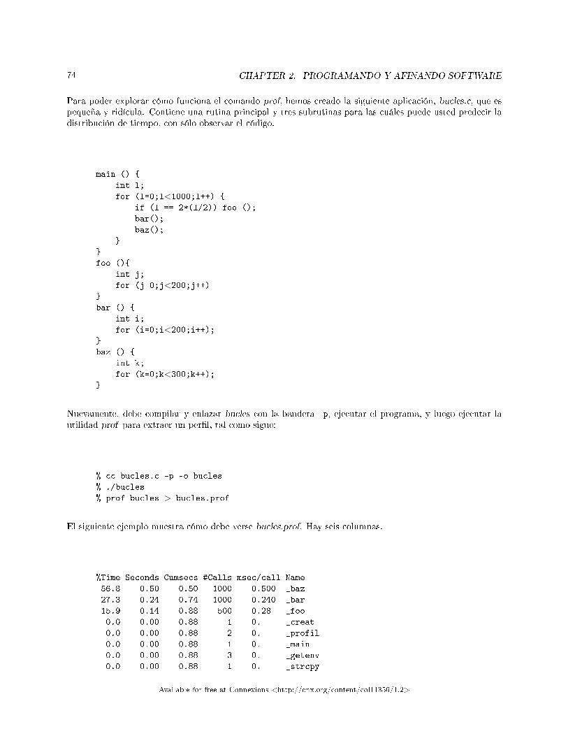
74 CHAPTER 2. PROGRAMANDO Y AFINANDO SOFTWARE
Para poder explorar cómo funciona el comando prof, hemos creado la siguiente aplicación, bucles.c, que espequeña y ridícula. Contiene una rutina principal y tres subrutinas para las cuáles puede usted predecir ladistribución de tiempo, con sólo observar el código.
main () {
int l;
for (l=0;l<1000;l++) {
if (l == 2*(l/2)) foo ();
bar();
baz();
}
}
foo (){
int j;
for (j=0;j<200;j++)
}
bar () {
int i;
for (i=0;i<200;i++);
}
baz () {
int k;
for (k=0;k<300;k++);
}
Nuevamente, debe compilar y enlazar bucles con la bandera �p, ejecutar el programa, y luego ejecutar lautilidad prof para extraer un per�l, tal como sigue:
% cc bucles.c -p -o bucles
% ./bucles
% prof bucles > bucles.prof
El siguiente ejemplo muestra cómo debe verse bucles.prof. Hay seis columnas.
%Time Seconds Cumsecs #Calls msec/call Name
56.8 0.50 0.50 1000 0.500 _baz
27.3 0.24 0.74 1000 0.240 _bar
15.9 0.14 0.88 500 0.28 _foo
0.0 0.00 0.88 1 0. _creat
0.0 0.00 0.88 2 0. _profil
0.0 0.00 0.88 1 0. _main
0.0 0.00 0.88 3 0. _getenv
0.0 0.00 0.88 1 0. _strcpy
Available for free at Connexions <http://cnx.org/content/col11356/1.2>
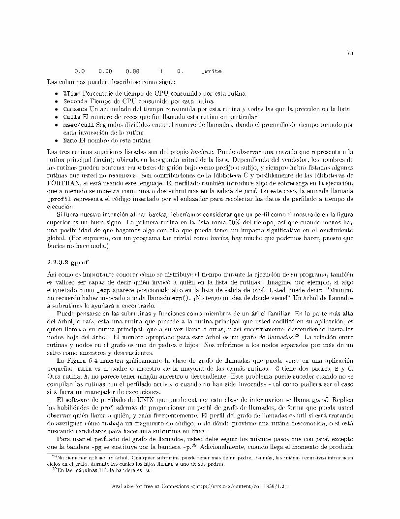
75
0.0 0.00 0.88 1 0. _write
Las columnas pueden describirse como sigue:
• %Time Porcentaje de tiempo de CPU consumido por esta rutina• Seconds Tiempo de CPU consumido por esta rutina• Cumsecs Un acumulado del tiempo consumida por esta rutina y todas las que la preceden en la lista• Calls El número de veces que fue llamada esta rutina en particular• msec/call Segundos divididos entre el número de llamadas, dando el promedio de tiempo tomado por
cada invocación de la rutina• Name El nombre de esta rutina
Las tres rutinas superiores listadas son del propio bucles.c. Puede observar una entrada que representa a larutina principal (main), ubicada en la segunda mitad de la lista. Dependiendo del vendedor, los nombres delas rutinas pueden contener caracteres de guión bajo como pre�jo o su�jo, y siempre habrá listadas algunasrutinas que usted no reconozca. Son contribuciones de la biblioteca C y posiblemente de las bibliotecas deFORTRAN, si está usando este lenguaje. El per�lado también introduce algo de sobrecarga en la ejecución,que a menudo se muestra como una o dos subrutinas en la salida de prof. En este caso, la entrada llamada_profil representa el código insertado por el enlazador para recolectar los datos de per�lado a tiempo deejecución.
Si fuera nuestra intención a�nar bucles, deberíamos considerar que un per�l como el mostrado en la �gurasuperior es un buen signo. La primera rutina en la lista toma 50% del tiempo, así que cuando menos hayuna posibilidad de que hagamos algo con ella que pueda tener un impacto signi�cativo en el rendimientoglobal. (Por supuesto, con un programa tan trivial como bucles, hay mucho que podemos hacer, puesto quebucles no hace nada.)
2.2.3.2 gprof
Así como es importante conocer cómo se distribuye el tiempo durante la ejecución de su programa, tambiénes valioso ser capaz de decir quién invocó a quién en la lista de rutinas. Imagine, por ejemplo, si algoetiquetado como _exp aparece posicionado alto en la lista de salida de prof. Usted puede decir: "Mmmm,no recuerdo haber invocado a nada llamado exp(). ½No tengo ni idea de dónde viene!� Un árbol de llamadosa subrutinas le ayudará a encontrarlo.
Puede pensarse en las subrutinas y funciones como miembros de un árbol familiar. En la parte más altadel árbol, o raíz, está una rutina que precede a la rutina principal que usted codi�có en su aplicación; esquien llama a su rutina principal, que a su vez llama a otras, y así sucesivamente, descendiendo hasta losnodos hoja del árbol. El nombre apropiado para este árbol es un grafo de llamadas.28 La relación entrerutinas y nodos en el grafo es uno de padres e hijos. Nos referimos a los nodos separados por más de unsalto como ancestros y descendientes.
La Figura 6-4 muestra grá�camente la clase de grafo de llamadas que puede verse en una aplicaciónpequeña. main es el padre o ancestro de la mayoría de las demás rutinas. G tiene dos padres, E y C.Otra rutina, A, no parece tener ningún ancestro o descendiente. Este problema puede suceder cuando no secompilan las rutinas con el per�lado activo, o cuando no han sido invocadas - tal como pudiera ser el casosi A fuera un manejador de excepciones.
El software de per�lado de UNIX que puede extraer esta clase de información se llama gprof. Replicalas habilidades de prof, además de proporcionar un per�l de grafo de llamados, de forma que pueda ustedobservar quién llama a quién, y cuán frecuentemente. El per�l del grafo de llamadas es útil si está tratandode averiguar cómo trabaja un fragmento de código, o de dónde proviene una rutina desconocida, o si estábuscando candidatos para hacer una subrutina en línea.
Para usar el per�lado del grafo de llamados, usted debe seguir los mismos pasos que con prof, exceptoque la bandera �pg se sustituye por la bandera �p.29 Adicionalmente, cuando llega el momento de producir
28No tiene por qué ser un árbol. Cualquier subrutina puede tener más de un padre. Es más, las rutinas recursivas introducenciclos en el grafo, durante los cuales los hijos llaman a uno de sus padres.
29En las máquinas HP, la bandera es �G.
Available for free at Connexions <http://cnx.org/content/col11356/1.2>
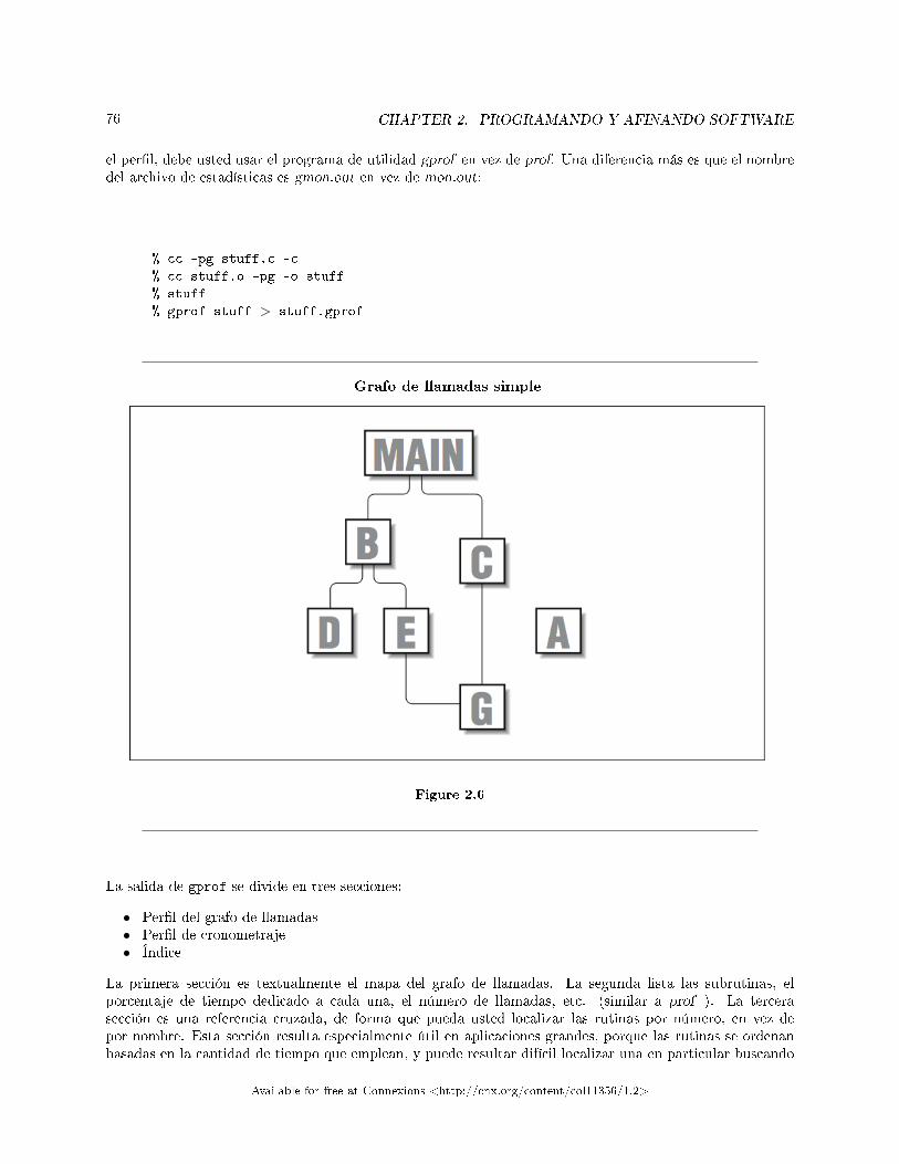
76 CHAPTER 2. PROGRAMANDO Y AFINANDO SOFTWARE
el per�l, debe usted usar el programa de utilidad gprof en vez de prof. Una diferencia más es que el nombredel archivo de estadísticas es gmon.out en vez de mon.out:
% cc -pg stuff.c -c
% cc stuff.o -pg -o stuff
% stuff
% gprof stuff > stuff.gprof
Grafo de llamadas simple
Figure 2.6
La salida de gprof se divide en tres secciones:
• Per�l del grafo de llamadas• Per�l de cronometraje• Índice
La primera sección es textualmente el mapa del grafo de llamadas. La segunda lista las subrutinas, elporcentaje de tiempo dedicado a cada una, el número de llamadas, etc. (similar a prof ). La tercerasección es una referencia cruzada, de forma que pueda usted localizar las rutinas por número, en vez depor nombre. Esta sección resulta especialmente útil en aplicaciones grandes, porque las rutinas se ordenanbasadas en la cantidad de tiempo que emplean, y puede resultar difícil localizar una en particular buscando
Available for free at Connexions <http://cnx.org/content/col11356/1.2>
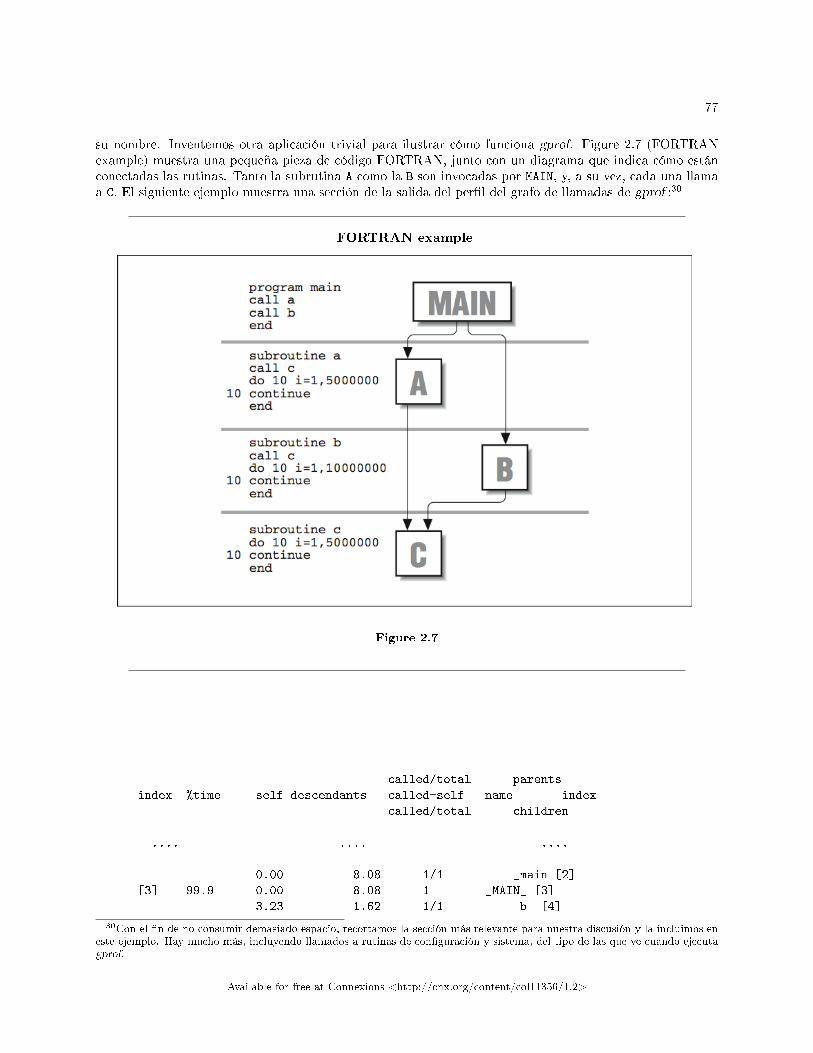
77
su nombre. Inventemos otra aplicación trivial para ilustrar cómo funciona gprof. Figure 2.7 (FORTRANexample) muestra una pequeña pieza de código FORTRAN, junto con un diagrama que indica cómo estánconectadas las rutinas. Tanto la subrutina A como la B son invocadas por MAIN, y, a su vez, cada una llamaa C. El siguiente ejemplo muestra una sección de la salida del per�l del grafo de llamadas de gprof :30
FORTRAN example
Figure 2.7
called/total parents
index %time self descendants called+self name index
called/total children
.... .... ....
0.00 8.08 1/1 _main [2]
[3] 99.9 0.00 8.08 1 _MAIN_ [3]
3.23 1.62 1/1 _b_ [4]
30Con el �n de no consumir demasiado espacio, recortamos la sección más relevante para nuestra discusión y la incluimos eneste ejemplo. Hay mucho más, incluyendo llamados a rutinas de con�guración y sistema, del tipo de las que ve cuando ejecutagprof.
Available for free at Connexions <http://cnx.org/content/col11356/1.2>
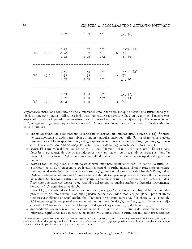
78 CHAPTER 2. PROGRAMANDO Y AFINANDO SOFTWARE
1.62 1.62 1/1 _a_ [5]
-----------------------------------------------
3.23 1.62 1/1 _MAIN_ [3]
[4] 59.9 3.23 1.62 1 _b_ [4]
1.62 0.00 1/2 _c_ [6]
-----------------------------------------------
1.62 1.62 1/1 _MAIN_ [3]
[5] 40.0 1.62 1.62 1 _a_ [5]
1.62 0.00 1/2 _c_ [6]
-----------------------------------------------
1.62 0.00 1/2 _a_ [5]
1.62 0.00 1/2 _b_ [4]
[6] 39.9 3.23 0.00 2 _c_ [6]
Emparedada entre cada conjunto de líneas punteadas está la información que describe una rutina dada y surelación respecto a padres e hijos. Es fácil decir qué rutina representa cada bloque, porque el mismo estádesplazado más a la izquierda que los otros. Los padres se listan arriba, los hijos abajo. Como sucedió conprof, se agregaron guiones bajos a las etiquetas.31 A continuación se muestra una descripción de cada unade las columnas:
• index Observará que cada nombre de rutina tiene asociado un número entre corchetes ([n]). Se tratade una referencia cruzada para ubicar rutina en cualquier parte del per�l. Si, por ejemplo, está ustedbuscando en el bloque que describe _MAIN_ y quiere saber más acerca de sus hijos, digamos _a_, puedeencontrarlo recorriendo hacia abajo la parte izquierda de la página en busca de su índice, [5].
• %time El signi�cado del campo %time es un poco diferente del que tiene para prof. En este casodescribe el porcentaje de tiempo gastado en esta rutina mas el tiempo gastado en todos sus hijos. Leproporciona una forma rápida de determinar dónde encontrar las partes más ocupadas del grafo dellamadas.
• self Listado en segundos, la columna self tiene diferentes signi�cados para los padres, la rutina encuestión y sus hijos. Comenzando con la entrada central -la rutina misma- el valor self muestra cuántotiempo global se dedicó a la rutina. En el caso de _b_, por ejemplo, esta cantidad fue de 3.23 segundos.Cada entrada en la columna self muestra la cantidad de tiempo que puede atribuirse a llamadas desdelos padres. Si observa la rutina _c_, por ejemplo, verá que consumió un tiempo total de 3.23 segundos.Pero note que tuvo dos padres: 1.62 segundos del tiempo se pueden atribuir a llamadas provenientesde _a_, y 1.62 segundos a las de _b_.Para el hijo, la cantidad self muestra cuánto tiempo se gastó ejecutando cada hijo, debido a llamadasprovenientes de esta rutina. Los hijos pueden haber consumido más tiempo global, pero el únicotiempo contabilizado es aquél atribuíble a llamadas desde esta subrutina. Por ejemplo, _c_ acumuló3.23 segundos globales, pero si observa en el bloque describiendo _b_, verá a _c_ listada como un hijocon sólo 1.62 segundos. Este fue el tiempo total gastado ejecutando _c_ del lado de _b_.
• descendants Como ocurren con la columna self, los vaores en la columna de descendientes tienendiferentes signi�cados para la rutina, sus padres y los hijos. Para la rutina misma, muestra el número
31Puede que haya observado que hay dos rutinas principales: _MAIN_ y _main. En un programa FORTRAN, _MAIN_ es laverdadera rutina principal, que es invocada como una subrutina por _main, que proporciona una biblioteca del sistema a tiempode enlace. Cuando per�la usted código en C, no verá _MAIN_.
Available for free at Connexions <http://cnx.org/content/col11356/1.2>
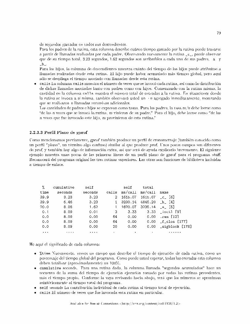
79
de segundos gastados en todos sus descendientes.Para los padres de la rutina, esta columna describe cuánto tiempo gastado por la rutina puede trazarsea partir de llamadas realizadas por cada padre. Observando nuevamente la rutina _c_, puede observarque de su tiempo total, 3.23 segundos, 1.62 segundos son atribuíbles a cada uno de sus padres, _a_ y_b_.Para los hijos, la columna de descendientes muestra cuánto del tiempo de los hijos puede atribuirse allamadas realizadas desde esta rutina. El hijo puede haber acumulado más tiempo global, pero aquísólo se despliega el tiempo asociado con llamadas desde esta rutina.
• calls La columna calls muestra el número de veces que se invocó cada rutina, así como la distribuciónde dichas llamadas asociadas tanto con padres como con hijos. Comenzando con la rutina misma, lacantidad en la columna calls muestra el número total de entradas a la rutina. En situaciones dondela rutina se invoca a sí misma, también observará usted un +n agregado inmediatamente, mostrandoque se realizaron n llamadas recursivas adicionales.Las cantidades de padres e hijos se expresan como tasas. Para los padres, la tasa m/n debe leerse como�de las n veces que se invocó la rutina, m vinieron de su padre.� Para el hijo, debe leerse como "de lasn veces que fue invocado este hijo, m provinieron de esta rutina.�
2.2.3.3 Per�l Plano de gprof
Como mencionamos previamente, gprof también produce un per�l de cronometraje (también conocido comoun per�l "plano", un término algo confuso) similar al que produce prof. Unos pocos campos son diferentesde prof, y también hay algo de información extra, así que será de ayuda explicarlo brevemente. El siguienteejemplo muestra unas pocas de las primeras líneas de un per�l plano de gprof para el programa stu�.Reconocerá del programa original las tres rutinas superiores. Las otras son funciones de biblioteca incluidasa tiempo de enlace.
% cumulative self self total
time seconds seconds calls ms/call ms/call name
39.9 3.23 3.23 2 1615.07 1615.07 _c_ [6]
39.9 6.46 3.23 1 3230.14 4845.20 _b_ [4]
20.0 8.08 1.62 1 1620.07 3235.14 _a_ [5]
0.1 8.09 0.01 3 3.33 3.33 _ioctl [9]
0.0 8.09 0.00 64 0.00 0.00 .rem [12]
0.0 8.09 0.00 64 0.00 0.00 _f_clos [177]
0.0 8.09 0.00 20 0.00 0.00 _sigblock [178]
... .... .... . . . ......
He aquí el signi�cado de cada columna:
• %time Nuevamente, vemos un campo que describe el tiempo de ejecución de cada rutina, como unporcentaje del tiempo global del programa. Como puede usted esperar, todas las entradas esta columnadeben totalizar (aproximadamente) un 100%.
• cumulative seconds. Para una rutina dada, la columna llamada "segundos acumulados" hace unrecuento de la suma del tiempo de ejecución ejecución tomado por todas las rutinas precedentes,más el tiempo propio. Conforme la vaya revisando hacia abajo, verá que los números se aproximanasintóticamente al tiempo total del programa.
• self seconds La contribución individual de cada rutina al tiempo total de ejecución.• calls El número de veces que fue invocada esta rutina en particular.
Available for free at Connexions <http://cnx.org/content/col11356/1.2>
80 CHAPTER 2. PROGRAMANDO Y AFINANDO SOFTWARE
• self ms/call Los segundos gastados adentro de la rutina, dividido entre el número de llamadas. Ellonos da una duración promedio del tiempo tomado por cada invocación a la rutina. La cantidad estámedida en milisegundos.
• total ms/call Los segundos gastados adentro de la rutina más sus descendientes, dividido entre elnúmero de llamados.
• name El nombre de la rutina. Observe que de nuevo aparece aquí el número de referencia cruzada.
2.2.3.4 Acumulando los Resultados de Varias Corridas de gprof
Es posible acumular estadísticas provenientes de múltiples corridas, de forma que obtenga usted una instan-tánea del comportamiento del programa con una variedad de conjuntos de datos. Por ejemplo, digamos quequiere usted per�lar una aplicación - llamémosla bar � con tres conjuntos de datos distintos. Puede realizarlas corridas separadamente, guardando los archivos gmon.out conforme las ejecuta, y luego combinar losresultados en un solo per�l al terminar:
% f77 -pg bar.f -o bar
% bar < data1.input
% mv gmon.out gmon.1
% bar < data2.input
% mv gmon.out gmon.2
% bar < data3.input
% gprof bar -s gmon.1 gmon.2 gmon.out > gprof.summary.out
En el per�l de ejemplo, cada corrida crea un nuevo archivo gmon.out que luego renombramos para que no seaencimado por el siguiente. Al �nal, gprof combina la información de cada uno de los archivos de datos paraproducir un per�l sumario de bar en el archivo gprof.summary.out. Adicionalmente (aunque no se muestraaquí), gprof crea un archivo llamado gmon.sum que contiene los datos mezclados a partir de los tres archivosde datos originales. gmon.sum tiene el mismo formato que gmon.out, de forma que pueda usted usarlo comoentrada para producir otros per�les mezclados si así lo requiere.
Al menos en forma, la salida del per�l mezclado luce exactamente igual que el de una corrida individual.Pero hay un par de cosas interesantes que debemos señalar. Por un lado, la rutina main parece haber sidoinvocada más de una vez - de hecho, una vez por cada corrida. Además, dependiendo de la aplicación, lasmúltiples ejecuciones tienden o bien a suavizar el contorno del per�l, o bien a exagerar sus características.Puede imaginar cómo es que esto sucede. Si se está invocando constantemente una única rutina, mientrasque las otras vienen y van conforme cambian los datos de entrada, ésta toma una importancia creciente ensus esfuerzos de a�nación.
2.2.3.5 Unas Pocas Palabras Acerca de la Exactitud
En aquellos procesadores que se ejecutan a 600 MHz o más, el tiempo que transcurre entre muestras de 60Hz y 100 Hz es una verdadera eternidad. Es más, puede que experimente usted errores de cuanti�cacióncuando la frecuencia de muestreo es �ja, como es el caso en muestras de 1/100 y 1/60 de segundo. Para usarun ejemplo exagerado, asumamos que la línea de tiempo en Figure 2.8 (Errores de cuanti�cación al per�lar)muestra invocaciones alternadas a dos subrutinas, BAR y FOO. Las marcas cronométricas representan lospuntos de muestreo del per�lado.
Available for free at Connexions <http://cnx.org/content/col11356/1.2>
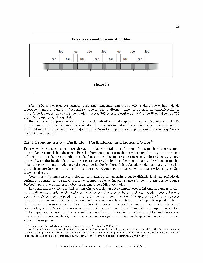
81
Errores de cuanti�cación al per�lar
Figure 2.8
BAR y FOO se ejecutan por turnos. Pero BAR toma más tiempo que FOO. Y dado que el intervalo demuestreo es muy cercano a la frecuencia en que ambas se alternan, tenemos un error de cuanti�cación: lamayoría de las muestras se están tomando mientras FOO se está ejecutando. Así, el per�l nos dice que FOO
usa más tiempo de CPU que BAR.Hemos descrito y probado los per�ladores de subrutinas reales que han estado disponibles en UNIX
durante años. En muchos casos, los vendedores tienen herramientas mucho mejores, ya sea a la venta ogratis. Si usted está haciendo un trabajo de a�nación serio, pregunte a su representante de ventas qué otrasherramientas le ofrece.
2.2.4 Cronometraje y Per�lado - Per�ladores de Bloques Básicos32
Existen varias buenas razones para desear un nivel de detalle más �ne que el que puede obtener usandoun per�lador a nivel de subrutina. Para los humanos que tratan de entender cómo se usa una subrutinao función, un per�lador que indique cuáles líneas de código fuente se están ejecutando realmente, y cuána menudo, resulta invaluable; unas pocas pistas acerca de dónde enfocar sus esfuerzos de a�nación puedenahorrarle mucho tiempo. Además, tal tipo de per�lador le ahora el descubrimiento de que una optimizaciónparticularmente inteligente no resulta en diferencia alguna, porque la colocó en una sección cuyo códigonunca se ejecuta.
Como parte de una estrategia global, un per�lador de subrutinas puede dirigirlo hacia un puñado derutinas que contabilizan la mayor parte del tiempo de ejecución, pero se necesita de un per�lador de bloquesbásicos33 para que pueda usted obtener las líneas de código asociadas.
Los per�ladores de bloques básicos también proporcionan a los compiladores la información que necesitanpara realizar sus propias optimizaciones. Muchos compiladores trabajan a ciegas: pueden reestructurar ydesenrollar ciclos, pero no pueden decir cuándo merece la pena hacerlo. Y lo que es todavía peor, a veceslas optimizaciones mal ubicadas ½tienen el efecto adverso de volver más lento el código! Ello puede deberseal gravamen a que se ve sometida la cache de instrucciones, a las pruebas innecesarias introducidas por elcompilador, o a hipótesis incorrectas acerca de qué camino tomará una bifurcación a tiempo de ejecución.Si el compilador puede interpretar automáticamente los resultados de un per�lador de bloques básicos, o sipuede usted proporcionarle algunos indicios, a menudo signi�ca un tiempo de ejecución reducido con pocoesfuerzo de su parte.
32This content is available online at <http://cnx.org/content/m38419/1.1/>.33Un bloque básico es una sección de código con un único punto de entrada y un único punto de salida. Si sabe cuántas veces
se entró al bloque, sabe cuántas veces se ejecutó cada sentencia en el bloque, lo cuál le está dando un per�l línea por línea. Elconcepto de bloque básico se explica con más detalle en (<http://cnx.org/content/m33690/latest/>)
Available for free at Connexions <http://cnx.org/content/col11356/1.2>
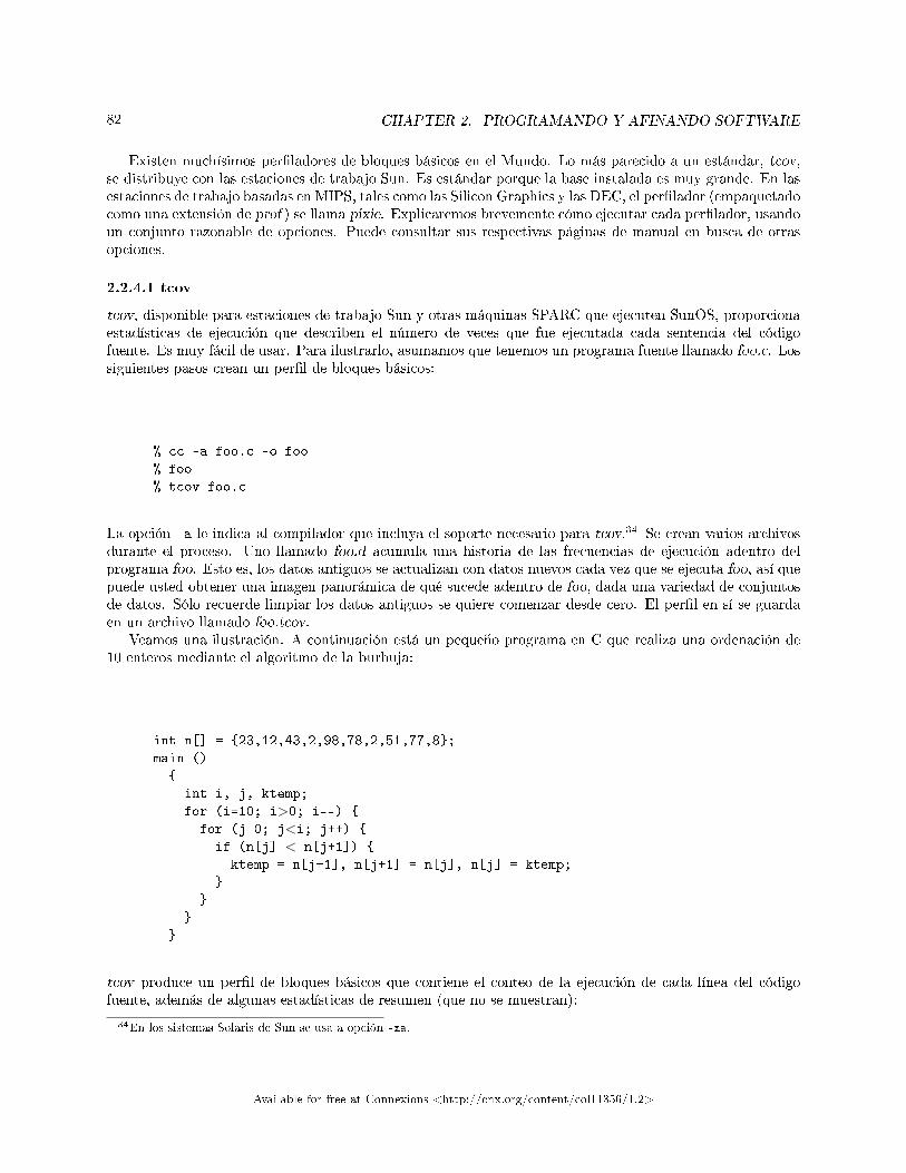
82 CHAPTER 2. PROGRAMANDO Y AFINANDO SOFTWARE
Existen muchísimos per�ladores de bloques básicos en el Mundo. Lo más parecido a un estándar, tcov,se distribuye con las estaciones de trabajo Sun. Es estándar porque la base instalada es muy grande. En lasestaciones de trabajo basadas en MIPS, tales como las Silicon Graphics y las DEC, el per�lador (empaquetadocomo una extensión de prof ) se llama pixie. Explicaremos brevemente cómo ejecutar cada per�lador, usandoun conjunto razonable de opciones. Puede consultar sus respectivas páginas de manual en busca de otrasopciones.
2.2.4.1 tcov
tcov, disponible para estaciones de trabajo Sun y otras máquinas SPARC que ejecuten SunOS, proporcionaestadísticas de ejecución que describen el número de veces que fue ejecutada cada sentencia del códigofuente. Es muy fácil de usar. Para ilustrarlo, asumamos que tenemos un programa fuente llamado foo.c. Lossiguientes pasos crean un per�l de bloques básicos:
% cc -a foo.c -o foo
% foo
% tcov foo.c
La opción -a le indica al compilador que incluya el soporte necesario para tcov.34 Se crean varios archivosdurante el proceso. Uno llamado foo.d acumula una historia de las frecuencias de ejecución adentro delprograma foo. Esto es, los datos antiguos se actualizan con datos nuevos cada vez que se ejecuta foo, así quepuede usted obtener una imagen panorámica de qué sucede adentro de foo, dada una variedad de conjuntosde datos. Sólo recuerde limpiar los datos antiguos se quiere comenzar desde cero. El per�l en sí se guardaen un archivo llamado foo.tcov.
Veamos una ilustración. A continuación está un pequeño programa en C que realiza una ordenación de10 enteros mediante el algoritmo de la burbuja:
int n[] = {23,12,43,2,98,78,2,51,77,8};
main ()
{
int i, j, ktemp;
for (i=10; i>0; i--) {
for (j=0; j<i; j++) {
if (n[j] < n[j+1]) {
ktemp = n[j+1], n[j+1] = n[j], n[j] = ktemp;
}
}
}
}
tcov produce un per�l de bloques básicos que contiene el conteo de la ejecución de cada línea del códigofuente, además de algunas estadísticas de resumen (que no se muestran):
34En los sistemas Solaris de Sun se usa a opción �xa.
Available for free at Connexions <http://cnx.org/content/col11356/1.2>
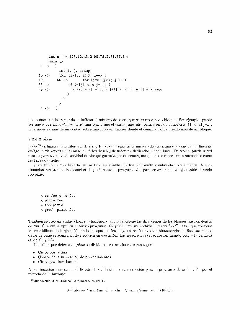
83
int n[] = {23,12,43,2,98,78,2,51,77,8};
main ()
1 -> {
int i, j, ktemp;
10 -> for (i=10; i>0; i--) {
10, 55 -> for (j=0; j<i; j++) {
55 -> if (n[j] < n[j+1]) {
23 -> ktemp = n[j+1], n[j+1] = n[j], n[j] = ktemp;
}
}
}
1 -> }
Los números a la izquierda le indican el número de veces que se entró a cada bloque. Por ejemplo, puedever que a la rutina sólo se entró una vez, y que el conteo más alto ocurre en la condición n[j] < n[j+1].tcov muestra más de un conteo sobre una línea en lugares donde el compilador ha creado más de un bloque.
2.2.4.2 pixie
pixie 35 es ligeramente diferente de tcov. En vez de reportar el número de veces que se ejecuta cada línea decódigo, pixie reporta el número de ciclos de reloj de máquina dedicados a cada línea. En teoría, puede ustedusarlos para calcular la cantidad de tiempo gastada por sentencia, aunque no se representan anomalías comolas fallas de cache.
pixie funciona �pixi�cando� un archivo ejecutable que fue compilado y enlazado normalmente. A con-tinuación mostramos la ejecución de pixie sobre el programa foo para crear un nuevo ejecutable llamadofoo.pixie:
% cc foo.c -o foo
% pixie foo
% foo.pixie
% prof -pixie foo
También se creó un archivo llamado foo.Addrs, el cual contiene las direcciones de los bloques básicos dentrode foo. Cuando se ejecuta el nuevo programa, foo.pixie, crea un archivo llamado foo.Counts , que contienela contabilidad de la ejecución de los bloques básicos cuyas direcciones están almacenadas en foo.Addrs. Losdatos de pixie se acumulan de ejecución en ejecución. Las estadísticas se recuperan usando prof y la banderaespecial �pixie.
La salida por defecto de pixie se divide en tres secciones, como sigue:
• Ciclos por rutina• Conteo de la invocación de procedimientos• Ciclos por línea básica
A continuación mostramos el listado de salida de la tercera sección para el programa de ordenación por elmétodo de la burbuja:
35duendecillo, si se traduce literalmente. N. del T.
Available for free at Connexions <http://cnx.org/content/col11356/1.2>

84 CHAPTER 2. PROGRAMANDO Y AFINANDO SOFTWARE
procedure (file) line bytes cycles % cum %
main (foo.c) 7 44 605 12.11 12.11
_cleanup (flsbuf.c) 59 20 500 10.01 22.13
fclose (flsbuf.c) 81 20 500 10.01 32.14
fclose (flsbuf.c) 94 20 500 10.01 42.15
_cleanup (flsbuf.c) 54 20 500 10.01 52.16
fclose (flsbuf.c) 76 16 400 8.01 60.17
main (foo.c) 10 24 298 5.97 66.14
main (foo.c) 8 36 207 4.14 70.28
.... .. .. .. ... ...
Aquí puede usted ver tres entradas para la rutina principal de foo.c, además de un número de rutinas debibliotecas del sistema. Las entradas muestran el número de línea asociado y el número de ciclos de máquinadedicados a ejecutar dicha línea, conforme se corrió el programa. Por ejemplo, la línea 7 de foo.c tomó 605ciclos (12% del tiempo de ejecución).
2.2.5 Cronometraje y Per�lado - Memoria Virtual36
Además de tener un impacto negativo en el rendimiento debido a las fallas de cache, el sistema de memoriavirtual puede disminuir la velocidad de ejecución de su programa, si es demasiado grande para caber en lamemoria del sistema, o está compitiendo con otros trabajos grandes por usar una memoria escasa.
En la mayoría de las implementaciones de UNIX, el sistema operativo descarga automáticamente al áreade intercambio parte de las páginas de aquellos programas demasiado grandes para caber en la memoriadisponible. No arrojan el programa completo; sólo sucede cuando la memoria está completamente justa, ocuando su programa ha estado inactivo durante un rato. En tal caso, algunas páginas individuales se ponenen el área de intercambio para su recuperación posterior. En primer término, debe usted estar consciente deque esto está sucediendo, si es que todavía no se ha percatado. Y en segundo término, si está pasando, lospatrones de acceso a memoria se tornan críticos. Cuando las referencias sean muy dispersas, su tiempo deejecución quedará dominado completamente por la E/S a disco.
Si lo planea con anticipación, puede hacer que un sistema de memoria virtual trabaje para usted cuandosu programa sea demasiado grande para alojarse en la memoria física de la máquina. Las técnicas sonexactamente las mismas que las empleadas para a�nar una aplicación sin espacio en memoria principaladministrada por software, o bucles anidados. Consiste en "bloquear" las referencias a memoria, de formaque los datos consumidos en los vecinos usen una mayor porción de cada página de memoria virtual antesde regresarla a disco para hacer espacio para otra. 37
2.2.5.1 Calibrando el Tamaño de su Programa y el Tamaño de la Memoria
¾Cómo puede asegurar que se ha quedado sin espacio en memoria principal? Hay varias formas de comprobarla paginación en la máquina, pero tal vez la prueba más sencilla es comparar el tamaño de su programa conla cantidad de memoria disponible. Esto se hace mediante el comando size:
36This content is available online at <http://cnx.org/content/m38424/1.1/>.37Examinamos las técnicas para bloqueos en el Capítulo 8.
Available for free at Connexions <http://cnx.org/content/col11356/1.2>
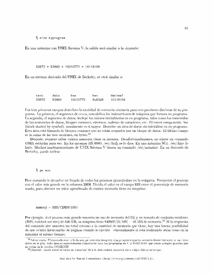
85
% size myprogram
En una máquina con UNIX Sistema V, la salida será similar a la siguiente:
53872 + 53460 + 10010772 = 10118104
En un sistema derivado del UNIX de Berkeley, se verá similar a:
text data bss hex decimal
53872 53460 10010772 9a63d8 10118104
Los tres primeros campos describen la cantidad de memoria necesaria para tres porciones distintas de su pro-grama. La primera, el segmento de texto, contabiliza las instrucciones de máquina que forman su programa.La segunda, el segmento de datos, incluye los valores inicializados en su programa, tales como los contenidosde las sentencias de datos, bloques comunes, externos, cadenas de caracteres, etc. El tercer componente, bss(block started by symbol), usualmente es el mayor. Describe un área de datos sin inicializar en su programa.Esta área está formada de bloques comunes que no están ocupados por un bloque de datos. El último campoes la suma de las tres secciones, en bytes.38
Después, requiere saber cuánta memoria tiene su sistema. Desafortunadamente, no existe un comandoUNIX estándar para eso. En los sistemas RS/6000, /etc/lscfg se lo dice. En una máquina SGI, /etc/hinv lohace. Muchas implementaciones de UNIX Sistema V tienen un comando /etc/memsize. En un derivado deBerkeley, puede teclear:
% ps aux
Este comando le devuelve un listado de todos los procesos ejecutándose en la máquina. Encuentre el procesocon el valor más grande en la columna %MEM. Divida el valor en el campo RSS entre el porcentaje de memoriausado, para obtener un valor aproximado de cuánta memoria tiene su máquina:
memory = RSS/(%MEM/100)
Por ejemplo, si el proceso más grande muestra un uso de memoria del 5% y un tamaño de conjunto residente(RSS, resident set size) de 840 KB, su máquina tiene 840000/(5/100) = 16 MB de memoria.39 Si la respuestadel comando size muestra un total cercano a la cantidad de memoria que tiene, hay una buena posibilidadde que ocurra intercambio de páginas cuando lo ejecute - especialmente si está realizando otras cosas en lamáquina al mismo tiempo.
38Advertencia: El comando size no le da una panorámica completa si su programa aparta memoria dinámicamente, o mantienedatos en la pila. Esta área es especialmente importante para los programas en C y FORTRAN que crean arreglos grandes queno están en la sección COMMON.
39½También puede usted reiniciar su máquina! Ella le dirá cuánta memoria tiene disponible al arranque.
Available for free at Connexions <http://cnx.org/content/col11356/1.2>
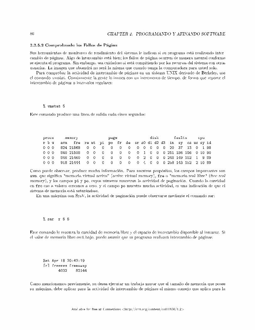
86 CHAPTER 2. PROGRAMANDO Y AFINANDO SOFTWARE
2.2.5.2 Comprobando los Fallos de Página
Sus herramientas de monitoreo de rendimiento del sistema le indican si su programa está realizando inter-cambio de páginas. Algo de intercambio está bien; los fallos de página ocurren de manera natural conformese ejecuta el programa. Sin embargo, sea cuidadoso si está compitiendo por los recursos del sistema con otrosusuarios. La imagen que obtendrá no será la misma que cuando tenga la computadora para usted solo.
Para comprobar la actividad de intercambio de páginas en un sistema UNIX derivado de Berkeley, useel comando vmstat. Comúnmente la gente lo invoca con un incremento de tiempo, de forma que reporte elintercambio de páginas a intervalos regulares:
% vmstat 5
Este comando produce una línea de salida cada cinco segundos:
procs memory page disk faults cpu
r b w avm fre re at pi po fr de sr s0 d1 d2 d3 in sy cs us sy id
0 0 0 824 21568 0 0 0 0 0 0 0 0 0 0 0 20 37 13 0 1 98
0 0 0 840 21508 0 0 0 0 0 0 0 1 0 0 0 251 186 156 0 10 90
0 0 0 846 21460 0 0 0 0 0 0 0 2 0 0 0 248 149 152 1 9 89
0 0 0 918 21444 0 0 0 0 0 0 0 4 0 0 0 258 143 152 2 10 89
Como puede observar, produce mucha información. Para nuestros propósitos, los campos importantes sonavm, que signi�ca "memoria virtual activa" (active virtual memory), fre o "memoria real libre" (free realmemory), y los campos pi y po, cuyos números muestran la actividad de paginación. Cuando la cantidaden fre cae a valores cercanos a cero, y el campo po muestra mucha actividad, es una indicación de que elsistema de memoria está saturándose.
En una máquina con SysV, la actividad de paginación puede observarse mediante el comando sar:
% sar -r 5 5
Este comando le muestra la cantidad de memoria libre y el espacio de intercambio disponible al instante. Siel valor de memoria libre está bajo, puede asumir que su programa realizará intercambio de páginas:
Sat Apr 18 20:42:19
[r] freemem freeswap
4032 82144
Como mencionamos previamente, su desea ejecutar un trabajo mayor que el tamaño de memoria que poseesu máquina, debe aplicar para la actividad de intercambio de páginas el mismo consejo que aplica para la
Available for free at Connexions <http://cnx.org/content/col11356/1.2>
87
actividad de cache.40 Trate de minimizar el tamaño de incremento en los bucles de su código, y cuando nopueda, bloquear las referencias a memoria ayudará muchísimo.
Una nota sobre las herramientas de monitoreo de rendimiento de la memoria: debe comprobar con elvendedor de su estación de trabajo si tienen disponible alguna herramienta además de vmstat o sar. Puedeque exista alguna herramienta mucho más so�sticada (y tal vez grá�ca) que le ayude a comprender cómo esque su programa utiliza la memoria.
2.2.6 Cronometraje y Per�lado - Notas de Cierre41
Hemos visto algunas de las herramientas para cronometraje y per�lado. Incluso aunque parezca que hemoscubierto mucho, hay otras clases de per�ladores que debiéramos cubrir - medidas de fallas de cache, análisisde dependencias a tiempo de ejecución, medición de operaciones de punto �otante por segundo, y variasmás. Estos per�les son buenos cuando está buscando ciertas anomalías en particular, tales como fallas decache o uso de las líneas de espera de punto �otante. En algunas máquinas existen per�ladores para estascantidades, pero no están ampliamente distribuidos.
Algo para tener en mente: cuando per�le código, a veces obtiene una visión muy limitada de la formaen que se usa el programa. Ello es especialmente cierto si puede realizar muchos tipos de análisis paramuchos conjuntos distintos de datos de entrada. Trabajar con sólo uno o dos per�les puede darle una vistadistorsionada de cómo opera el código en su conjunto. Imagine el siguiente escenario: alguien le invita adar su primer paseo en automóvil. Está sentado en el asiento del pasajero con un cuaderno y una pluma, yregistra todo lo que sucede. Sus observaciones incluyen cosas tales como:
• El radio siempre está encendido.• Los limpiaparabrisas nunca se usan.• El automóvil sólo se mueve hacia adelante.
El peligro es que, dado lo limitado de su óptica acerca la forma en que se opera el auto, puede que quieradesconectar la perilla de encendido y apagado del radio, quitar los limpiaparabrisas y eliminar el engranajede reversa. ½Ello se convertirá en una verdadera sorpresa para la siguiente persona que intente estacionaren reversa el auto en un día lluvioso! El punto es que a menos que sea usted cuidadoso al recolectar datosde todos los tipos de usos posibles, puede que no tenga una panorámica real de cómo opera el programa.Un único per�l es bueno para a�nar un banco de pruebas, pero puede olvidar algún detalle importante enuna aplicación multipropósito. Peor todavía, si usted lo optimiza para un caso y lo mutila para otro, puedeproducir más daño que bene�cio.
Per�lar, como hemos visto en este capítulo, es bastante mecánico. A�nar requiere de introspección.Es justo advertirle que no siempre es una actividad provechosa. A veces pone todo su empeño en unamodi�cación inteligente que, contrariamente a lo esperado, incrementa el tiempo de ejecución. ½Ah! ¾Quésalió mal? Dependerá usted de sus herramientas de per�lado para contestarse esta pregunta.
2.2.7 Cronometraje y Per�lado - Ejercicios42
Exercise 2.2.7.1Per�le el siguiente programa usando gprof. ¾Hay alguna forma de decir cuánto del tiempo gastadoen la rutina c se debe a llamadas recursivas?
40Por cierto, ¾está recibiendo el mensaje �Out of memory?� Si está ejecutando csh, pruebe a teclear unlimit para ver si elmensaje desaparece. De otro modo, puede signi�car que no tiene su�ciente espacio de intercambio disponible para ejecutar eltrabajo.
41This content is available online at <http://cnx.org/content/m38425/1.1/>.42This content is available online at <http://cnx.org/content/m38426/1.1/>.
Available for free at Connexions <http://cnx.org/content/col11356/1.2>
88 CHAPTER 2. PROGRAMANDO Y AFINANDO SOFTWARE
main()
{
int i, n=10;
for (i=0; i<1000; i++) {
c(n);
a(n);
}
}
c(n)
int n;
{
if (n > 0) {
a(n-1);
c(n-1);
}
}
a(n)
int n;
{
c(n);
}
Exercise 2.2.7.2Per�le un código ingenieril (que haga uso intensivo de números de punto �otante) con la opti-mización completa activa y no activa. ¾Cómo cambia el per�l? ¾Puede explicar por qué?
Exercise 2.2.7.3Escriba un programa para determinar la sobrecarga que representa invocar a getrusage y etime.Aparte del tiempo de procesador que consumen, ¾cómo altera el rendimiento de la aplicación, elhecho de invocar demasiado a menudo una llamada al sistema para cronometraje?
2.3 Eliminando el Desorden
2.3.1 Eliminando el Desorden - Introducción43
Hemos visto el código desde el punto de vista del compilador, y cómo per�lar código para encontrar las zonasproblemáticas. Esta información es buena, pero si aún no está satisfecho con el rendimiento de cierto código,seguro piensa qué más hacer con él. Una posibilidad es que su código sea demasiado obtuso para que elcompilador pueda optimizarlo apropiadamente: código excesivo, excesiva modularización o incluso "mejoras"debidas a procesos de optimización previos pueden desordenar su código y confundir a los compiladores. Seconsidera desorden a todo aquello que contribuye al tiempo de ejecución sin contribuir a la respuesta. Vieneen dos formas:Cosas que contribuyen a la sobrecargaLlamados a subrutinas, referencias indirectas a memoria, pruebas adentro de bucles, pruebas excesivas,conversiones de tipos, variables preservadas innecesariamenteCosas que restringen la �exibilidad del compiladorLlamados a subrutinas, referencias indirectas a memoria, pruebas adentro de bucles, apuntadores ambiguos
43This content is available online at <http://cnx.org/content/m38428/1.3/>.
Available for free at Connexions <http://cnx.org/content/col11356/1.2>
89
No se trata de un error que algunos elementos aparezcan repetidos en ambas listas. Tanto la invocaciónde subrutinas como el uso de sentencias condicionales adentro de bucles pueden perjudicarlo, al tomar muchotiempo y generar barreras � lugares del programa donde las instrucciones que aparecen antes no puedenentremezclarse de forma segura con las instrucciones que aparecen después, al menos no sin un gran cuidado.El objetivo de este capítulo es mostrarle cómo eliminar el desorden, de forma que pueda reestructurar todoaquello que está mal y lograr la ejecución más rápida posible. Hemos eliminado unos cuantos tópicos quedebieran estar aquí, especialmente aquellos relativos a referencias a memoria, y los colocamos en capítulosposteriores donde se tratan como temas separados.
Antes de comenzar, queremos recordarle: conforme busca usted formas de mejorar lo que tiene, mantengaojos y mente abiertos a la posibilidad de que pueda existir una manera fundamentalmente mejor de hacer algo-una técnica de ordenación más e�ciente, un generador de números aleatorios, etc. Un algoritmo diferentepuede aportarle mayor incremento de velocidad que a�nar el existente. Analizar tales algoritmos está másallá del alcance de este libro, pero lo que estamos discutiendo aquí debe ayudarle a reconocer el "buen"código, o ayudarle a codi�car un nuevo algoritmo que le de el mejor rendimiento.
2.3.2 Eliminando el Desorden - Llamado a Subrutinas44
Una empresa típica está llena de aterrorizantes ejemplos de sobrecarga. Digamos que un departamento hapreparado una pila de papelería, que debe completar otro departamento. ¾Qué debe usted de hacer paratransferir tal trabajo? Primero, debe asegurarse que la parte que le tocó hacer esté completa; no puedepedirles que lo acepten si los materiales que requieren no están listos. Después, necesitará empaquetar losmateriales - datos, formas, números de cuenta, etc. Y �nalmente viene la transferencia o�cial. Una vez querecibió lo que usted les envió, el otro departamento debe desempacarlo, hacer su trabajo, reempaquetarlo yenviarlo de vuelta.
Se malgasta una gran cantidad de tiempo moviendo trabajos entre departamentos. Por supuesto, si lasobrecarga es mínima comparada con la cantidad de trabajo útil que se hace, no hay gran problema. Peropudiera ser más e�ciente llevar a cabo los trabajos pequeños adentro del mismo departamento. Lo mismopuede a�rmarse de la invocación de subrutinas y funciones. Si sólo entra y sale de los módulos muy de vezen cuando, la sobrecarga de guardar los valores en los registros y preparar la lista de argumentos no resultarásigni�cativa. Sin embargo, si está invocando repetidamente unas pocas subrutinas pequeñas, la sobrecargapuede mantenerlas siempre encabezando la lista del per�l. Puede que fuera mejor si el trabajo permanecieradonde está, en la subrutina emisora de la llamada.
Adicionalmente, los llamados a subrutinas inhiben la �exibilidad del compilador. Si se presenta la opor-tunidad, usted quiere que su compilador tenga la �exibilidad su�ciente para entremezclar instrucciones queno son dependientes las unas de las otras. Y tales instrucciones se encuentran en ambas caras de un llamadoa subrutina, en el invocador y en el invocado. Pero la oportunidad se pierde cuando el compilador no puedeemparejarlas dentro de subrutinas y funciones. Y así, instrucciones que perfectamente pudieran solaparse,permanecen en sus respectivos lados de la barrera arti�cial.
Puede ser de ayuda que ilustremos el reto que representan las fronteras de las subrutinas mediante unejemplo exagerado. Los siguientes bucles se ejecutan muy bien en una amplia variedad de procesadores:
DO I=1,N
A(I) = A(I) + B(I) * C
ENDDO
El código de abajo realiza los mismos cálculos, pero observe qué hemos hecho:
44This content is available online at <http://cnx.org/content/m38429/1.2/>.
Available for free at Connexions <http://cnx.org/content/col11356/1.2>
90 CHAPTER 2. PROGRAMANDO Y AFINANDO SOFTWARE
DO I=1,N
CALL MADD (A(I), B(I), C)
ENDDO
SUBROUTINE MADD (A,B,C)
A = A + B * C
RETURN
END
Cada iteración invoca a una subrutina para realizar una pequeña cantidad de trabajo, que antes estabaubicado adentro del ciclo. Este es un ejemplo particularmente doloroso, porque involucra cálculos de punto�otante. La pérdida de paralelismo resultante, junto con la sobrecarga debida al llamado al procedimiento,puede producir código que se ejecuta 100 veces más lento. Recuerde, tales operaciones se colocan en líneas deespera, y toma cierta cantidad de tiempo "de recuperación" antes de que el rendimiento alcance siquiera unaoperación por ciclo de reloj. Si son pocas las operaciones de punto �otante que se realizan entre llamados asubrutinas, el tiempo gastado en llenar y vaciar las líneas de espera se volverá muy importante.
La invocación de subrutinas y funciones complica la habilidad que tiene el compilador de manejar e�cien-temente variables COMMON y external, retrasando su almacenamiento en memoria hasta el último momentoposible. El compilador usa registros para almacenar los valores "vivos" de muchas variables. Cuando re-aliza una llamada, el compilador no puede saber cuáles de las variables cambiarán en la subrutina queestá declarada como external o COMMON, y por ello se ve forzado a almacenar en memoria cualquier vari-able external o COMMON que haya sido modi�cada, de modo que la subrutina invocada pueda encontrarla.De igual modo, tras el retorno de la llamada, las mismas variables tienen que cargarse nuevamente en losregistros, porque el compilador no puede con�ar en las copias antiguas que residen en los registros. Lapenalización de guardar y recuperar variables puede ser substancial, especialmente si son muchas. Tambiénpuede resultar riesgoso si las variables que debieran ser locales fueron especi�cadas como external o COMMON,como sucede en el siguiente código:
COMMON /USELESS/ K
DO K=1,1000
IF (K .EQ. 1) CALL AUX
ENDDO
En este ejemplo, K se ha declarado como una variable COMMON. Sólo se usa como contador del ciclo do-loop,así que realmente no hay razón para que sea otra cosa que local. Sin embargo, dado que está en un bloqueCOMMON, la llamada a AUX obliga al compilador a almacenar y recargar K cada iteración. Ello se debe a quese desconocen los efectos laterales que la llamada puede producir.
Hasta aquí, pareciera como si estuviéramos abonando el camino para ½programas principales enormes, sinsubrutinas o funciones! En absoluto. La modularidad es importante para mantener compacto y comprensibleel código fuente. Y francamente, la necesidad de modularidad y facilidad de mantenimiento siempre es másimportante que la necesidad de pequeñas mejoras de rendimiento. Sin embargo, hay un par de enfoquesque permiten racionalizar los llamados a subrutinas, y que no requieren que usted abandone las técnicas decodi�cación modular: se trata de las macros y los procedimientos en línea.
Recuerde, si la función o subrutina hace una cantidad razonable de trabajo, no importará demasiado lasobrecarga debida a la invocación del procedimiento. Sin embargo, si una rutina pequeña aparece como un
Available for free at Connexions <http://cnx.org/content/col11356/1.2>
91
nodo hijo en una de las secciones más atareadas del grafo de llamados, puede que deba pensar en insertarlaen los lugares apropiados del programa.
2.3.2.1 Macros
Las Macros (o macroinstrucciones) son pequeños procedimientos que se substituyen en línea a tiempo decompilación. Al contrario que las subrutinas o funciones, que se incluyen una vez durante el proceso deenlazado, las macros se replican en cada lugar que se usan. Cuando el compilador lleva a cabo su primerapasada a lo largo de su programa, busca patrones que coincidan con las de�niciones previas de macros, ylas expande en línea. De hecho, en etapas posteriores, el compilador ve una macro expandida como si fueracódigo fuente creado por usted.
Las macros forman parte tanto de C como de FORTRAN (aunque la noción equivalente a una macro enFORTRAN, la función sentencia, ha sido vilipendiada por la comunidad FORTRAN y no sobrevivirá muchotiempo más).45 En los programas en lenguaje C, las macros se crean mediante una directiva #define, comose demuestra aquí:
#define promedio(x,y) ((x+y)/2)
main ()
{
float q = 100, p = 50;
float a;
a = promedio(p,q);
printf ("%f\n",a);}
El primer paso de compilación de un programa en C consiste en pasar por el preprocesador de C, cpp. Elloocurre automáticamente cuando usted invoca al compilador. cpp expande las sentencias #define en línea,reemplazando el patrón coincidente por la de�nición de la macro. En el programa de arriba, la sentencia:
a = promedio(p,q);
es reemplazada por:
a = ((p+q)/2);
Debe usted ser cuidadoso al de�nir la macro, porque literalmente reemplaza al patrón que cpp encuentra.Por ejemplo, si la de�nición de la macro decía:
#define multiplicar(a,b) (a*b)
45La función sentencia se ha eliminado de FORTRAN 90.
Available for free at Connexions <http://cnx.org/content/col11356/1.2>

92 CHAPTER 2. PROGRAMANDO Y AFINANDO SOFTWARE
y usted lo invocó como:
c = multiplicar(x+t,y+v);
la expansión resultante será x+t*y+v � que probablemente no es lo que usted pretendía.Si es usted un programador en C, puede que esté usando macros sin siquiera percatarse. Muchos archivos
de cabecera en C (.h) contienen de�niciones de macros. De hecho, algunas funciones "estándar" de bibliotecaen C en realidad son macros contenidas en tales archivos. Por ejemplo, la función getchar puede enlazarsecuando construye su programa. Si tiene una sentencia:
#include <stdio.h>
en su archivo, getchar se reemplazará con una de�nición de macro a tiempo de compilación, reemplazandola función de biblioteca de C.
También puede usted hacer que las macros de cpp trabajen para los programas en FORTRAN.46 Porejemplo, una versión FORTRAN del programa en C anterior pudiera verse así:
#define PROMEDIO(X,Y) ((X+Y)/2)
C
PROGRAM MAIN
REAL A,P,Q
DATA P,Q /50.,100./
A = PROMEDIO(P,Q)
WRITE (*,*) A
END
Sin algo de preparación, la sentencia #define será rechazada por el compilador de FORTRAN. El programadebe preprocesarse previamente mediante cpp para reemplazar el uso de PROMEDIO con su de�nición demacro. Ello convierte a la compilación en un procedimiento de dos pasos, pero que no debe ser una cargamayor, especialmente si está construyendo sus programas bajo el control del programa de utilidad make.También le sugerimos almacenar los programas en FORTRAN que contienen directivas para cpp mediantela nomenclatura �lename.F para distinguirlos de los programas FORTRAN sin adornos. Sólo asegúrese dehacer los cambios sólo a los archivos .F, y no a la salida de cpp. Así es como debe preprocesar los archivos.F de FORTRAN a mano:
% /lib/cpp -P < promedio.F > promedio.f
% f77 promedio.f -c
46Algunos programadores pre�eren usar para FORTRAN el preprocesador estándar de UNIX, m4 .
Available for free at Connexions <http://cnx.org/content/col11356/1.2>
93
El compilador de FORTRAN nunca ve el código original. En vez de ello, la de�nición de la macro se sustituyeen línea, tal y como si la hubiera tecleado usted mismo:
C
PROGRAM MAIN
REAL A,P,Q
DATA P,Q /50.,100./ A = ((P+Q)/2)
WRITE (*,*) A
END
Por cierto, algunos compiladores de FORTRAN también reconocen la extensión .F, haciendo innecesario elproceso en dos pasos. Si el compilador ve la extensión .F invoca automáticamente a cpp, y desecha el archivo.f intermedio. Trate de compilar un archivo .F en su computadora para ver si funciona.
También, tome conciencia de que la expansión de macros puede provocar que las líneas de código fuenteexcedan la columna 72, lo cuál hará que su compilador de FORTRAN reclame (o peor, que le pase de-sapercibido). Algunos compiladores soportan líneas de entrada más largas de 72 caracteres. En los compi-ladores de Sun la opción �e permite extender las líneas de entrada hasta 132 caracteres de longitud.
2.3.2.2 Procedimientos En Línea
Las de�niciones de macros tienden a ser muy cortas, usualmente de sólo una sentencia de longitud. A vecestiene usted porciones de código ligeramente más largas (pero no demasiado largas), que también puedenobtener bene�cio si se copian en línea, en vez de invocarse como subrutina o función. Nuevamente, la razónde hacerlo es eliminar la sobrecarga debida a la invocación de procedimientos, y exponer el paralelismo. Sisu compilador es capaz de de�nir subrutinas y funciones inline (en línea) al interior de los módulos que lasinvocan, entonces dispone de una forma muy natural y portátil de escribir código modular sin sufrir del costodebido a la invocación de la subrutina.
Dependiendo del vendedor, puede preguntarle al compilador si soporta la declaración de procedimientosen línea mediante:
• Especi�car desde la línea de comandos aquellas rutinas que deben insertarse en línea• Poner directivas para la declaración en línea dentro del código fuente• Permitir que el compilador decida automáticamente qué poner en línea
Las directivas y las opciones de la línea de comandos del compilador no están estandarizadas, así que deberárevisar la documentación de su compilador. Desafortunadamente, puede que nuevamente descubra que nohay tal característica (�nuevamente,� siempre nuevamente), o que es una característica extra que por la quedeberá pagar. La tercera forma de declaración en línea de la lista, la automática, sólo la tienen disponibleunos pocos vendedores. La declaración en línea automática depende de que el compilador sea so�sticado ypueda ver las de�niciones de varios módulos a la vez.
Unas últimas palabras de precaución respecto a la colocación de procedimientos en línea. Es fácil exageraren su uso. Si todo termina enquistado en el cuerpo o en sus padres, el ejecutable resultante puede ser tangrande que repetidamente desborde la cache de instrucciones y se convierta en una pérdida de rendimientoneto. Nuestro consejo es que use la información de invocador/invocado que le proporcionan los per�ladorespara tomar decisiones inteligentes acerca de la ubicación en línea, en vez de tratar de aplicarlo a cadasubrutina que genere. De nuevo, los mejores candidatos generalmente son aquellas rutinas pequeñas que seinvocan muy a menudo.
Available for free at Connexions <http://cnx.org/content/col11356/1.2>
94 CHAPTER 2. PROGRAMANDO Y AFINANDO SOFTWARE
2.3.3 Eliminando el Desorden - Bifurcaciones47
A veces a las personas les lleva una semana tomar una decisión, así que no deberíamos quejarnos si unacomputadora se toma unas pocas decenas de nanosegundos para hacerlo. Sin embargo, si aparece unasentencia selectiva en alguna sección altamente visitada del código, puede que usted acabe cansado de losretrasos que produce. Hay dos enfoques básicos para reducir el impacto de estas bifurcaciones:
• Racionalizarla.• Enviarla a los suburbios computacionales. Particularmente, mandarla afuera de los bucles.
here48 mostramos algunas formas fáciles de reorganizar condicionales, de forma que se ejecuten más rápida-mente.
2.3.4 Eliminando el Desorden - Bifurcaciones con Ciclos49
Los códigos numéricos usualmente gastan la mayoría de su tiempo de ejecución en ciclos, así que usted noquiere nada adentro de tales ciclos que no deba estar ahí, especialmente una sentencia selectiva. Y no sólose trata de que las sentencias selectivas entorpezcan el trabajo con instrucciones extras; también puedenforzar un orden estricto sobre las iteraciones de un ciclo. Por supuesto, no siempre pueden evitarse talescondicionales. A veces, sin embargo, la gente las pone adentro de los ciclos para procesar eventos quepudieran manejarse por separado, o incluso ignorarse.
Para hacerle retroceder unos pocos años, el siguiente código muestra un ciclo con una prueba para unvalor cercano a cero:
PARAMETER (SMALL = 1.E-20)
DO I=1,N
IF (ABS(A(I)) .GE. SMALL) THEN
B(I) = B(I) + A(I) * C
ENDIF
ENDDO
La idea era que si el factor, A(I), era razonablemente pequeño, no se justi�caba realizar la matemática enel centro del ciclo. Dado que las operaciones de punto �otante no se colocaban en �las de espera en muchasmáquinas, una comparación y un salto eran más económicos; la prueba ahorraba tiempo. En un procesadorCISC más antiguo o en los primeros RISC, una comparación y un salto probablemente aún ahorren tiempo.Pero en otras arquitecturas, cuesta mucho menos realizar la matemática y evitar la prueba. Eliminar labifurcación elimina una dependencia de control y permite que el compilador ponga en �la de espera másoperaciones aritméticas. Por supuesto, la respuesta puede cambiar ligeramente si se elimina la prueba. Luegose convierte en una cuestión de cuán signi�cativa es la diferencia. He aquí otro ejemplo donde no se requierede una bifurcación. El bucle encuentra el valor absoluto de cada elemento en un arreglo:
DO I=1,N
IF (A(I) .LT. 0.) A(I) = -A(I)
ENDDO
47This content is available online at <http://cnx.org/content/m38430/1.2/>.48"Eliminating Clutter - Branches With Loops" <http://cnx.org/content/m33723/latest/>49This content is available online at <http://cnx.org/content/m38439/1.2/>.
Available for free at Connexions <http://cnx.org/content/col11356/1.2>

95
Pero, ¾por qué realizar la prueba? En muchas máquinas, es más rápido aplicar la operación abs() a cadaelemento del arreglo.
Debemos, empero, hacerle una advertencia: si está programando en C, el valor absoluto fabs(), es unllamado a subrutina. En este caso particular, le conviene más mantener el condicional adentro del ciclo.50
Aún en aquellos casos en que no pueda deshacerse del condicional, todavía quedan cosas que puede hacerpara minimizar la pérdida de rendimiento. Primero, debemos aprender a reconocer cuáles condicionalesdentro de los bucles pueden reestructurase y cuáles no. Las sentencias selectivas adentro de bucles caen envarias categorías:
• Condicionales invariantes en el ciclo• Condicionales dependientes del índice del ciclo• Condicionales independientes del ciclo• Condicionales dependientes del ciclo• Reducciones• Condicionales que trans�eren el control
Revisémoslas una por una.
2.3.4.1 Condicionales Invariantes en el Ciclo
El siguiente ciclo contiene una prueba invariante:
DO I=1,K
IF (N .EQ. 0) THEN
A(I) = A(I) + B(I) * C
ELSE
A(I) = 0.
ENDIF
ENDDO
�Invariante� signi�ca que el resultado siempre es el mismo. Sin importar lo que suceda con las variables A,B, C, e I, el valor de N no cambia, ni tampoco lo hará el resultado del resto.
Usted puede reestructurar el ciclo, poniendo la prueba fuera y replicando el cuerpo del ciclo dos veces- una para el caso de que la prueba sea verdadera, y la otra para el resultado falso, como en el ejemplosiguiente:
IF (N .EQ. 0) THEN
DO I=1,K
A(I) = A(I) + B(I) * C
ENDDO
ELSE
DO I=1,K
A(I) = 0
50La representación de la máquina de un número de punto �otante comienza con un bit de signo. Si el bit es cero, el númeroes positivo. Si es 1, el número es negativo. La función de valor absoluto más rápida es aquella que simplemente aplique un "Y"al bit de signo. Véanse los macros en /usr/include/macros.h y /usr/include/math.h.
Available for free at Connexions <http://cnx.org/content/col11356/1.2>
96 CHAPTER 2. PROGRAMANDO Y AFINANDO SOFTWARE
ENDDO
ENDIF
El efecto en el tiempo de ejecución es dramático. No sólo hemos eliminado K-1 copias de la prueba, tambiénhemos asegurado que los cálculos en el centro del ciclo no tengan dependencias de control sobre la sentenciaselectiva, y por tanto es mucho más fácil que el compilador lo ponga en una �la de espera.
Recordamos haber ayudado a alguien a optimizar un programa con ciclos que contenían condicionalessimilares. Comprobaban si debía imprimirse la salida del depurador adentro de cada iteración, o bienproducir un ciclo altamente optimizable. No podemos culpar a la persona por no observar cuánto reducíaesto la velocidad del programa. El rendimiento no era importante en ese momento. El programador sólotrataba de lograr que el código produjera respuestas correctas. Pero después, cuando comenzó a importarel rendimiento, limpiando condicionales invariantes fuimos capaces de acelerar el programa en un factor de100.
2.3.4.2 Condicionales Dependientes del Indice del Ciclo
Para los condicionales dependientes del índice del ciclo, la prueba es verdadera sólo para ciertos rangos delas variables usadas como índice del ciclo. Y no siempre es cierto o falso, como en otros condicionales queya revisamos, pero cambia de acuerdo a un patrón apreciable, uno que puede usarse a nuestro favor. Elsiguiente ciclo tiene dos variables índice, I y J.
DO I=1,N
DO J=1,N
IF (J .LT. I)
A(J,I) = A(J,I) + B(J,I) * C
ELSE
A(J,I) = 0.0
ENDIF
ENDDO
ENDDO
Observe cómo la sentencia selectiva divide las iteraciones en dos conjuntos distintos: aquéllas en las cuáleses verdadero y aquéllas en las que es falso. Puede usted tomar ventaja de que tal cosa sea predecible, parareestructurar el bucle en varios bucles - cada uno personalizado para una partición distinta:
DO I=1,N
DO J=1,I-1
A(J,I) = A(J,I) + B(J,I) * C
ENDDO
DO J=I,N
A(J,I) = 0.0
ENDDO
ENDDO
Available for free at Connexions <http://cnx.org/content/col11356/1.2>

97
La nueva versión resultará más rápida casi siempre, con la posible excepción del caso en que N tenga un valorpequeño, como 3, en cuyo caso hemos creado un mayor desorden. Pero aun en tal caso, el ciclo probablementetendrá un impacto pequeño en el tiempo total de ejecución, del que hubiera tenido si se dejaba tal como estácodi�cado.
2.3.4.3 Condicionales Independientes del Ciclo
Sería bueno que pudiera optimizar cada ciclo, particionándolo. Pero muy a menudo, el condicional nodepende directamente del valor de las variables índice. Aunque una variable índice esté involucrada en eldireccionamiento de un arreglo, no crea por adelantado un patrón reconocible - por lo menos no uno quepueda usted observar cuando está escribiendo el programa. He aquí uno de tales ciclos:
DO I=1,N
DO J=1,N
IF (B(J,I) .GT. 1.0) A(J,I) = A(J,I) + B(J,I) * C
ENDDO
ENDDO
NO hay mucho que pueda hacer con este tipo de condicional. Pero dado que cada iteración es independiente,puede desenrollar el ciclo, o bien realizarlo en paralelo.
2.3.4.4 Condicionales Dependientes del Ciclo
Cuando el condicional se basa en un valor que cambia con cada iteración del ciclo, al compilador no le quedamás opción que ejecutar el código exactamente tal y como se escribió. Por ejemplo, el siguiente ciclo tieneuna sentencia selectiva con una recursividad escalar interna:
DO I=1,N
IF (X .LT. A(I)) X = X + B(I)*2.
ENDDO
No puede usted saber en qué forma actuará la bifurcación en la siguiente iteración hasta que no hayaejecutado la actual. Para reconocer la dependencia, trate de desenrollar ligeramente el ciclo manualmente.Si no puede comenzar la segunda prueba hasta haber �nalizado la primera, tiene un condicional dependientedel ciclo. Puede que quiera revisar este tipo de bucles en busca de formas de eliminar el valor que cambiade iteración a iteración.
2.3.4.5 Reducciones
Mantenga la vista atenta en busca de ciclos en los cuales la sentencia selectiva está aplicando una funciónmax o min a un arreglo. Se trata de una reducción, así llamada porque reduce todo un arreglo a un resultadoescalar (por cierto, el ejemplo previo también fue una reducción). De nuevo, estamos un poco por delante denosotros mismos, pero dado que estamos hablando acerca de sentencias selectivas adentro de bucles, quierointroducir un truco para reestructurar las reducciones del tipo max y min para exponer un mayor paralelismo.El siguiente ciclo busca el valor máximo, z, en el arreglo a, recorriendo todos los elementos uno a la vez:
Available for free at Connexions <http://cnx.org/content/col11356/1.2>

98 CHAPTER 2. PROGRAMANDO Y AFINANDO SOFTWARE
for (i=0; i<n; i++)
z = a[i] > z ? a[i] : z;
Tal como está escrito es recursivo, como el bucle de la sección previa. Requiere usted el resultado de unaiteración dada antes de que pueda proceder con la siguiente. Sin embargo, y dado que estamos buscando elmayor elemento en todo el arreglo, y dado que será el mismo elemento (esencialmente) sin importar dóndelo hallemos, podemos reestructurar el ciclo para comprobar varios elementos a la vez (asumiendo que n esdivisible de forma entera entre 2, y que no incluya el ciclo precondicionante):
z0 = 0.;
z1 = 0.;
for (i=0; i< n-1; i+=2) {
z0 = z0 < a[i] ? a[i] : z0;
z1 = z1 < a[i+1] ? a[i+1] : z1;
}
z = z0 < z1 ? z1 : z0;
¾Observa cómo calcula el nuevo ciclo dos valores máximos en cada iteración? Estos máximos se comparanluego uno con otro, y el ganador se convierte en el nuevo valormax o�cial. Es análogo a la ronda de semi�nalesen un torneo de ping-pong. El ciclo anterior consistía en dos jugadores compitiendo a la vez mientras que elresto se sentaba a su alrededor; en cambio, el nuevo ciclo ejecuta varios encuentros simultáneos. En generalesta optimización en particular no es adecuada para codi�carse a mano. En los procesadores paralelos, elcompilador realiza la reducción a su propio modo. Si usted lo codi�có de forma similar a este ejemplo, puedeque esté limitando inadvertidamente la �exibilidad del compilador en un sistema paralelo.
2.3.4.6 Condicionales que Trans�eren el Control
Detengámonos por un segundo. ¾Ha notado cierta similaridad en todos los bucles hasta ahora? Sólo hemosbuscado un tipo de condicional, la asignación condicional, esto es, la reasignación de una variable basados enel resultado de la prueba. Por supuesto, no todo condicional termina en una asignación. Existen sentenciasque trans�eren el control de �ujo, tales como llamados a subrutinas o sentencias goto. En el siguienteejemplo, el programador está comprobando cuidadosamente antes de dividir entre cero:
Pero esta prueba tiene un impacto extremadamente negativo en el rendimiento, porque fuerza la ejecuciónde las iteraciones precisamente en el orden en que se escriben:
DO I=1,N
DO J=1,N
IF (B(J,I) .EQ. 0 ) THEN
PRINT *,I,J
STOP
ENDIF
A(J,I) = A(J,I) / B(J,I)
Available for free at Connexions <http://cnx.org/content/col11356/1.2>

99
ENDDO
ENDDO
Evitar este tipo de pruebas es una de las razones por las cuales los diseñadores del estándar de punto �otantedel IEEE agregaron las trampas (traps) en operaciones tales como dividir entre cero. El uso de trampaspermite al programador dentro de una sección de código de rendimiento crítico, lograr un rendimientomáximo sin necesidad de detectar cuándo ocurre un error.
2.3.5 Eliminando el Desorden - Otras Formas de Desorden51
El desorden puede asumir muchas formas. Considere que en las secciones previas hemos batallado con grandespiezas de basura como las que puede usted encontrar en el armario de su sala: una tabla de planchar, palosde hockey y palos de billar. Ahora nos dedicaremos a cosas más pequeñas: una goma de borrar, una pelotade tenis y el sombrero que nadie usa. Aquí queremos mencionar unos cuantos. De entrada pedimos disculpaspor cambiar los temas tanto, ½pero así es la naturaleza de limpiar un armario!
2.3.5.1 Conversiones de Tipos de Datos
Las sentencias que incluyen conversiones de tipos a tiempo de ejecución producen algo de penalización delrendimiento cada vez que se ejecutan. Si la sentencia se localiza en una porción muy activa del programa,la penalización total puede resultar signi�cativa.
Las personas tienen sus razones para escribir aplicaciones que mezclan tipos. A menudo es cuestión deahorrar espacio de memoria, ancho de banda de memoria, o tiempo. En el pasado, por ejemplo, los cálculosde doble precisión tomaban el doble que sus contrapartes de precisión sencilla, así que si alguno de talescálculos podía arreglarse para hacerse en precisión sencilla, bene�ciaba al rendimiento.52 Pero cualquiertiempo ahorrado realizando parte de los cálculos en precisión sencilla y la otra parte en doble precisión, debemedirse contra la sobrecarga adicional causada por las conversiones de tipos a tiempo de ejecución. En elsiguiente código, la suma de A(I) con B(I) tiene tipos mezclados:
INTEGER NUMEL, I
PARAMETER (NUMEL = 1000)
REAL*8 A(NUMEL)
REAL*4 B(NUMEL)
DO I=1,NUMEL
A(I) = A(I) + B(I)
ENDDO
En cada iteración, B(I) debe convertirse a doble precisión antes de que pueda ocurrir la suma. Usted no vela conversión en el código fuente, pero está ahí, y consume tiempo.
Advertencia para los programadores de C: en el libro de C de Kernighan y Ritchie (K&R) C, todos loscálculos de punto �otante que aparecen en los programas son en doble precisión - incluso si todas las variablesinvolucradas están declaradas como �oat. Es posible que usted escriba una aplicación K&R completa en unaprecisión, si bien sufrirá la penalización derivada de muchas conversiones de tipos.
Otro error relacionado con los tipos de datos, es usar operaciones de caracteres en las pruebas de lassentencias IF. En muchos sistemas, las operaciones sobre caracteres tienen un rendimiento más pobre que
51This content is available online at <http://cnx.org/content/m38441/1.2/>.52Actualmente, los cálculos en precisión sencilla pueden tardar más tiempo que aquellos en doble precisión de registro a
registro.
Available for free at Connexions <http://cnx.org/content/col11356/1.2>
100 CHAPTER 2. PROGRAMANDO Y AFINANDO SOFTWARE
sus equivalentes enteras, dado que se realizan mediante llamados a procedimientos. Por lo mismo, puedeque los optimizadores no revisen el código que usa variables de tipo caracter como buenos candidatos paraoptimización. Por ejemplo, el siguiente código:
DO I=1,10000
IF ( CHVAR(I) .EQ. 'Y' ) THEN
A(I) = A(I) + B(I)*C
ENDIF
ENDDO
puede escribirse mejor usando una variable entera para indicar si debe o no realizarse el cálculo:
DO I=1,10000
IF ( IFLAG(I) .EQ. 1 ) THEN
A(I) = A(I) + B(I)*C
ENDIF
ENDDO
Otra forma de escribir el código, asumiendo que la variable IFLAG fue 0 o 1, sería la siguiente:
DO I=1,10000
A(I) = A(I) + B(I)*C*IFLAG(I)
ENDDO
El último enfoque puede de hecho provocar mayor lentitud en algunos sistemas de cómputo, respecto alprimero, sobre todo si éste usa la variable entera en la sentencia IF.
2.3.5.2 Haciendo su Propia Eliminación de Subexpresiones Comunes
Hasta ahora le hemos dado a su compilador el bene�cio de la duda. La eliminación de subexpresionescomunes � la habilidad del compilador de reconocer patrones repetidos en el código, y reemplazar todosexcepto uno por una variable temporal- probablemente trabaje en su máquina con expresiones simples. En lasiguientes líneas de código, la mayoría de los compiladores reconocerán a+b como una subexpresión común:
c = a + b + d
e = q + a + b
que se transforma en:
Available for free at Connexions <http://cnx.org/content/col11356/1.2>
101
temp = a + b
c = temp + d
e = q + temp
La sustitución de a+b elimina algo de la aritmética. Si la expresión se reutiliza muchas veces, los ahor-ros pueden resultar signi�cativos. Sin embargo, es limitada la habilidad de un compilador para reconocersubexpresiones comunes, especialmente cuando tienen componentes múltiples o éstos aparecen permutados.Un compilador puede no ser capaz de reconocer que a+b+c y c+b+a son equivalentes.53 En las partes másimportantes del programa, debe usted considerar la eliminación a mano de las subexpresiones comunes enlas expresiones más complicadas. Ello garantiza que se realizará. En cierto modo compromete la belleza,pero hay algunas situaciones donde es mejor.
He aquí otro ejemplo en el cuál la función seno se invoca dos veces con el mismo argumento:
x = r*sin(a)*cos(b);
y = r*sin(a)*sin(b);
z = r*cos(a);
y que se convierte en:
temp = r*sin(a);
x = temp*cos(b);
y = temp*sin(b);
z = r*cos(a);
Hemos reemplazado uno de los llamados por una variable temporal. Estamos de acuerdo en que los ahorrosde eliminar la invocación de una función trascendente de entre cinco no nos hará ganar el Premio Nobel, peronos hace prestar atención a un punto importante: los compiladores típicamente no realizan la eliminaciónde subexpresiones comunes en subrutinas o llamados a funciones. El compilador no puede estar seguro queel llamado a la rutina no cambie el estado del argumento o de alguna otra variable que no puede ver.
La única ocasión en que un compilador puede eliminar subexpresiones comunes que contengan llamadosa funciones, es cuando son intrínsecas, como en FORTRAN. Y puede hacerse porque el compilador puedeasumir ciertas cosas acerca de los efectos laterales. Usted, por otra parte, puede ver adentro de las subruti-nas, lo cuál signi�ca que está mejor cali�cado que el compilador para agrupar subexpresiones comunes queinvolucren subrutinas o funciones.
2.3.5.3 Llevando a Cabo sus Propias Reubicaciones de Código
Donde mejor resulta llevar a cabo estas optimizaciones es adentro de los ciclos, porque es donde se concentratoda la actividad de un programa. Una de las mejores formas de recortar el tiempo de ejecución es moverlas instrucciones innecesarias o repetidas (invariantes) fuera del �ujo principal del código, a los suburbios.
53Y por causa del sobre�ujo y los errores de redondeo de punto �otante, en algunas situaciones pueden no ser equivalentes.
Available for free at Connexions <http://cnx.org/content/col11356/1.2>
102 CHAPTER 2. PROGRAMANDO Y AFINANDO SOFTWARE
En el caso de los bucles, se le denomina emerger instrucciones cuando se desplazan hacia la parte superiory sumergir instrucciones cuando se colocan en la parte inferior. He aquí un ejemplo:
DO I=1,N
A(I) = A(I) / SQRT(X*X + Y*Y)
ENDDO
que se convierte en:
TEMP = 1 / SQRT(X*X + Y*Y)
DO I=1,N
A(I) = A(I) * TEMP
ENDDO
Hicimos emerger una operación cara e invariante hacia afuera del ciclo, y asignamos el resultado a unavariable temporal. Observe también que hicimos una simpli�cación algebraica cuando intercambiamos unadivisión por la multiplicación por un inverso. La multiplicación se ejecutará mucho más rápido. Puede serque su compilador sea lo su�cientemente listo para hacer tales transformaciones por sí mismo, asumiendoque usted le haya instruido de que son transformaciones legales; pero sin rastrear el código ensambladorgenerado, no puede usted estar seguro. Por supuesto, si usted reacomoda el código a mano y el tiempo deejecución del ciclo súbitamente disminuye, sabrá que el compilador ha sido un lastre hasta entonces.
En ocasiones querrá usted sumergir una operación tras el ciclo. Usualmente, se trata de algún cálculorealizado cada iteración, pero cuyo resultado sólo se requiere al �nal. Para ilustrarlo, he aquí una clase deciclo distinto de los que hemos visto hasta ahora, uno que busca el caracter �nal en una cadena:
while (*p != ' ')
c = *p++;
se convierte en:
while (*p++ != ' ');
c = *(p-1);
La nueva versión del ciclo mueve la asignación de c más allá de la última iteración. Debemos admitir queesta transformación puede ser un logro para un compilador y que el ahorro no sea muy grande. Pero ilustrala idea de sumergir una operación muy bien.
Nuevamente, emerger y sumergir instrucciones para colocarlas afuera de ciclos es algo que su compiladorpuede que sea capaz de hacer. Pero a menudo usted puede reestructurar ligeramente los cálculos por símismo sólo con moverlos, y obtener un bene�cio todavía mayor.
Available for free at Connexions <http://cnx.org/content/col11356/1.2>
103
2.3.5.4 Manipulando los Elementos de un Arreglo en Bucles
Hay otra área donde debe usted con�ar en que el compilador hará lo correcto. Cuando emplee repetidamenteun elemento de un arreglo adentro de un bucle, querrá que se cargue una sola vez de la memoria. Tome elsiguiente bucle como un ejemplo. Reutiliza X(I) dos veces:
DO I=1,N
XOLD(I) = X(I)
X(I)= X(I) + XINC(I)
ENDDO
En realidad, los pasos encargados de recuperar X(I) sólo son subexpresiones comunes adicionales: un cálculode direcciones (posiblemente) y una operación de carga de memoria. Puede usted ver que la operación serepite al reescribir el ciclo ligeramente:
DO I=1,N
TEMP= X(I)
XOLD(I) = TEMP
X(I)= TEMP + XINC(I)
ENDDO
Los compiladores de FORTRAN deben reconocer que se está usando dos veces el mismo elemento X(I) yque por tanto sólo se requiere cargarlo una vez, pero no siempre un compilador es tan inteligente. A vecestiene usted que crear una variable escalar temporal para almacenar el valor de un elemento del arreglo enel cuerpo de un bucle. Esto es particularmente cierto cuando hay llamados a subrutinas o funciones en elciclo, o cuando alguna de las variables está declarada como external o COMMON. Asegúrese de emparejar lostipos entre las variables temporales y las otras variables, pues no quiere incurrir la sobrecarga derivada de laconversión de tipos sólo por estar "ayudando" al compilador. En el caso de los compiladores de C, el mismotipo de expresiones indexadas son un reto incluso mayor. Considere este código:
doinc(int xold[],int x[],int xinc[],int n)
{
for (i=0; i<n; i++) {
xold[i] = x[i];
x[i]= x[i] + xinc[i];
}
}
A menos que el compilador pueda ver las de�niciones de x, xinc y xold, debe asumir que son apuntadoresseñalando a la misma celda de almacenamiento, y repetir las operaciones de carga y almacenamiento. Eneste caso, introducir variables temporales para almacenar los valores de x, xinc, y xold es una optimizaciónque el compilador no es libre de hacer.
Available for free at Connexions <http://cnx.org/content/col11356/1.2>

104 CHAPTER 2. PROGRAMANDO Y AFINANDO SOFTWARE
Es interesante señalar que si bien usar variables escalares temporales en el ciclo es útil para las máquinasRISC y superescalares, no ayuda al código que se ejecuta sobre hardware paralelo. Un compilador paralelobusca oportunidades de eliminar los escalares o, cuando menos, de reemplazarlos con vectores temporales.Si ejecuta su código sobre una máquina paralela de vez en cuando, debe ser cuidadoso antes de introducirvariables escalares temporales en un ciclo. Una dudosa ganancia de rendimiento en una instancia puedeconvertirse en una pérdida de rendimiento real en otra.
2.3.6 Eliminando el Desorden - Notas de Cierre54
En este capítulo, introdujimos técnicas de a�nación que ayudan a eliminar el desorden de los programas- cualquier cosa que agregue tiempo de ejecución sin contribuir a hallar la respuesta. Hemos visto mu-chos ejemplos de técnicas de a�nación -su�cientes como para que usted se pregunte, "¾qué puede faltar?"Bueno, como veremos en los capítulos siguientes, todavía restan un par de formas en que podemos ayudaral compilador:
• Encontrando más paralelismo• Empleando la memoria tan e�cientemente como sea posible
A veces ello signi�cará realizar cambios que no son bonitos. Sin embargo, a menudo sí resultan rápidos.
2.3.7 Eliminando el Desorden - Ejercicios55
Exercise 2.3.7.1¾Cómo simpli�caría usted el siguiente ciclo condicional?
DO I=1,N
A(I) = A(I) * B
IF (I .EQ. N/2) A(I) = 0.
ENDDO
Exercise 2.3.7.2Cronometre el siguiente ciclo en su computadora, con y sin la condición. Ejecútelo con tresconjuntos de datos: uno con todos los valores A(I) menores que SMALL, uno con todos los valoresA(I) mayores que SMALL, y un tercero dividido en partes iguales. ¾Cuándo es mejor dejar la pruebaen el ciclo, si es el caso?
PARAMETER (SMALL = 1.E-20)
DO I=1,N
IF (ABS(A(I)) .GE. SMALL) THEN
B(I) = B(I) + A(I) * C
ENDIF
ENDDO
54This content is available online at <http://cnx.org/content/m38442/1.2/>.55This content is available online at <http://cnx.org/content/m38443/1.2/>.
Available for free at Connexions <http://cnx.org/content/col11356/1.2>
105
Exercise 2.3.7.3Escriba un programa sencillo que invoque a una subrutina sencilla en su ciclo interno. Cronometrela ejecución del programa. Luego dígale al compilador que compile la rutina en línea, y cronometrenuevamente. Finalmente, modi�que el código para realizar las operaciones en el cuerpo del ciclo,y cronometre el código. ¾Cuál opción se ejecutó más rápido? Puede que deba revisar el códigomáquina generado para imaginar el porqué.
2.4 Optimización de Ciclos
2.4.1 Optimización de Ciclos - Introducción56
En prácticamente todas las aplicaciones de alto rendimiento, es en los bucles donde se gasta la mayoría deltiempo de ejecución. here57 examinamos formas en las que los desarrolladores de la aplicación introdujerondesorden en los bucles, posiblemente haciéndolos ejecutarse más lento de lo necesario. En este capítulonos enfocaremos en técnicas para mejorar el rendimiento de tales ciclos "libres de desorden". A veces elcompilador es lo su�cientemente inteligente para generar las versiones más rápidas de los bucles, y otrasveces nos veremos en la necesidad de reescribirlos manualmente para ayudarle.
Es importante recordar que las modi�caciones que hagamos para mejorar el rendimiento del compilador,provocan otro desorden en el compilador. Cuando hace usted modi�caciones en nombre del rendimiento, debeasegurarse que éstas realmente ayudan, probando el rendimiento con y sin ellas. También, cuando se muevaa otra arquitectura, necesita asegurarse que cualquier modi�cación hecha no perjudique al rendimiento. Poresta razón, debe elegir sabiamente las modi�caciones que haga en pos del rendimiento. También debe dejarintacta la versión original (simple) del código, para probarla en nuevas arquitecturas. Si nota que el bene�cioderivado de las modi�caciones es pequeño, muy probablemente deba mantener el código en su versión mássimple y clara.
Revisaremos varias técnicas de optimización de bucles diferentes, incluyendo:
• Desenrollado de bucles• Optimización de bucles anidados• Intercambio de bucles• Optimización de las referencias a memoria• Bloqueo• Soluciones fuera del núcleo
Tal vez algún día sea posible que un compilador realice todas estas optimizaciones de bucles automáticamente.Es normal que el desenrollado de bucles se realice como parte de las optimizaciones de un compilador normal.Otras puede que deban incluirse mediante opciones explícitas del compilador al invocarlo. Cuando contemplehacer cambios manualmente, observe cuidadosamente cuáles de tales optimizaciones hace el compiladorautomáticamente. Y ejecute algunas pruebas para determinar si las optimizaciones del compilador son tanbuenas como aquellas realizadas a mano.
2.4.2 Optimización de Ciclos - Conteo de Operaciones58
Antes de que comience a reescribir el cuerpo de un bucle, o reorganizar el orden de los bucles, debe teneralguna idea de qué hace dicho cuerpo en cada iteración. Se llama conteo de operaciones al proceso de medirun ciclo para comprender la mezcla de operaciones. Necesitará contar el número de cargas, almacenamiento,operaciones de punto �otante, enteras, y llamados a bibliotecas por cada iteración del bucle. A partir
56This content is available online at <http://cnx.org/content/m38445/1.2/>.57"Eliminating Clutter - Introduction" <http://cnx.org/content/m33720/latest/>58This content is available online at <http://cnx.org/content/m38446/1.1/>.
Available for free at Connexions <http://cnx.org/content/col11356/1.2>
106 CHAPTER 2. PROGRAMANDO Y AFINANDO SOFTWARE
de este conteo, puede ver cuán bien se corresponde la mezcla de operaciones de un ciclo dado con lascapacidades del procesador. Por supuesto, el conteo de operaciones no garantiza que el compilador generaráuna representación e�ciente de un ciclo.59 Pero ello generalmente le proporcionará una percepción su�cientecomo para dirigir sus esfuerzos de a�nación.
Tenga en mente que una mezcla de instrucciones balanceada para una máquina puede no estarlo paraotra. Los procesadores que hay hoy día en el mercado pueden generalmente ejecutar alguna combinación deuna a cuatro instrucciones por ciclo de reloj. La aritmética de direcciones a menudo queda incrustada en lasinstrucciones que hacen referencia a memoria. Como el compilador puede reemplazar complicados cálculosde direcciones de bucles por expresiones simples (suponiendo que el patrón de direcciones es predecible), enocasiones puede usted ignorar la aritmética de direcciones cuando hace el conteo de operaciones.60
Revisemos unos cuantos bucles, y veamos qué podemos aprender acerca de la mezcla de instrucciones:
DO I=1,N
A(I,J,K) = A(I,J,K) + B(J,I,K)
ENDDO
Este bucle contiene una suma de punto �otante y tres referencias a memoria (dos cargas y un almace-namiento). Hay algunas expresiones complejas de indexación de arreglos, pero probablemente el compiladorlas simpli�que y pueda ejecutarlas en el mismo ciclo que aquellas de memoria y punto �otante. Para cadaiteración del ciclo, debemos incrementar la variable índice y probarla para determinar si éste se ha comple-tado.
Una tasa 3:1 de referencias a memoria respecto a operaciones de punto �otante sugiere que podemosaspirar a por lo menos 1/3 del rendimiento pico de punto �otante al ejecutar el bucle, a menos que haya másde un camino a la memoria. Son malas noticias, pero buena información. La tasa nos dice que debiéramosconsiderar primero la optimización de las referencias a memoria.
El bucle de abajo contiene una suma de punto �otante y dos operaciones a memoria - una carga y unalmacenamiento. El operando B(J) es invariante en el bucle, así que su valor sólo requiere de cargarse unavez, antes de la entrada al bucle:
DO I=1,N
A(I) = A(I) + B(J)
ENDDO
Nuevamente, nuestro rendimiento de punto �otante está limitado, pero no tan severamente como en el cicloanterior. La tasa de referencias a memoria respecto a operaciones de punto �otante es ahora de 2:1.
El siguiente ejemplo muestra un bucle con mejores perspectivas. Realiza multiplicaciones, a nivel deelementos, de números complejos y asigna los resultados de vuelta al primero de ellos. Hay seis operacionesa memoria (cuatro cargas y dos almacenamientos) y seis operaciones de punto �otante (dos sumas y cuatromultiplicaciones):
59Revise la salida en lenguaje ensamblador para estar seguro, la cuál puede estar introduciendo algo de desbordamiento.Para obtener un listado en lenguaje ensamblador en muchas máquinas, compile con la bandera �S. En las RS/6000, utilice labandera �qlist.
60El compilador reduce la complejidad de las expresiones de indexación del ciclo con una técnica llamada simpli�cación devariables de inducción. Véase (<http://cnx.org/content/m33690/latest/>).
Available for free at Connexions <http://cnx.org/content/col11356/1.2>
107
for (i=0; i<n; i++) {
xr[i] = xr[i] * yr[i] - xi[i] * yi[i];
xi[i] = xr[i] * yi[i] + xi[i] * yr[i];
}
Pareciera que este bucle está cercanamente balanceado para un procesador que pueda realizar el mismonúmero de operaciones de memoria y de punto �otante por ciclo. Sin embargo, puede que no sea así. Mu-chos procesadores realizan una multiplicación y una suma de punto �otante en una sola instrucción. Si elcompilador es lo su�cientemente bueno para reconocer que la suma-multiplicación es apropiada, este ciclopuede también verse limitado por las referencias a memoria; cada iteración se compilará en dos multiplica-ciones y dos multiplicaciones-sumas.
De nuevo, el conteo de operaciones es una forma simple de estimar cuán bien se mapean los requerimientosde un ciclo en las capacidades de una máquina. En el caso de muchos bucles, a menudo encontrará usted quesu rendimiento está dominado por las referencias a memoria, tal como vimos en los últimos tres ejemplos.Ello sugiere que la a�nación de las referencias a memoria es muy importante.
2.4.3 Optimización de Ciclos - Desenrollado Básico de Ciclos61
La forma más básica de optimización de bucles es desenrollarlos. Es algo tan básico que casi todos los compi-ladores actuales lo hacen automáticamente, si da la impresión de que repercutirá bené�camente. En nombredel desenrollado de bucles, se introdujo gran cantidad de desorden en los antiguos programas FORTRANahora cubiertos de polvo, que sólo sirve para confundir y despistar a los compiladores de hoy.
No estamos sugiriendo que deba usted desenrollar los bucles a mano. El propósito de esta sección esdoble: primero, una vez que esté familiarizado con el desenrollado de bucles, podrá reconocer código quedesenrolló el programador (no usted) tiempo atrás, y simpli�carlo; y segundo, necesita entender los conceptosdel desenrollado de bucles, de modo que cuando vea el código máquina generado, pueda reconocerlos.
El bene�cio primario de desenrollar bucles, es realizar más cálculos por iteración. Al �nal de cada una,el valor índice debe incrementarse, probarse y bifurcar el control de regreso al inicio del ciclo, si todavíafaltan iteraciones por procesar. Al desenrollar el bucle, hay menos "�nales de bucle" en la ejecución de cadaciclo. Desenrollar también reduce signi�cativamente el número total de bifurcaciones, y da al procesadormás instrucciones entre ellas (i.e., incrementa el tamaño de los bloques básicos).
A modo de ilustración, considere el siguiente bucle. Es una sentencia simple envuelta en un ciclo:
DO I=1,N
A(I) = A(I) + B(I) * C
ENDDO
Usted puede desenrollar el bucle, como haremos en el ejemplo siguiente, reescribiendo las mismas operacionesmediante menos iteraciones y con menos sobrecarga en el ciclo. Imagine cómo ayudará esto en cualquiercomputadora. Dado que los cálculos en una iteración no dependen de los cálculos en otras, los primerosy los segundos pueden ejecutarse juntos. En un procesador superescalar, ciertas porciones de estas cuatrosentencias pueden ejecutarse en paralelo:
61This content is available online at <http://cnx.org/content/m38449/1.2/>.
Available for free at Connexions <http://cnx.org/content/col11356/1.2>
108 CHAPTER 2. PROGRAMANDO Y AFINANDO SOFTWARE
DO I=1,N,4
A(I) = A(I) + B(I) * C
A(I+1) = A(I+1) + B(I+1) * C
A(I+2) = A(I+2) + B(I+2) * C
A(I+3) = A(I+3) + B(I+3) * C
ENDDO
Sin embargo, este ciclo no es exactamente el mismo que el anterior, pues se desenrolló cuatro veces, pero¾qué pasa si N no es divisible entre 4? Habrá una, dos o tres iteraciones sobrantes que no se ejecutarán. Paramanejar tales iteraciones extras, agregamos otro pequeño bucle para absorberlas. El ciclo extra se llama unbucle precondicionante:
II = IMOD (N,4)
DO I=1,II
A(I) = A(I) + B(I) * C
ENDDO
DO I=1+II,N,4
A(I) = A(I) + B(I) * C
A(I+1) = A(I+1) + B(I+1) * C
A(I+2) = A(I+2) + B(I+2) * C
A(I+3) = A(I+3) + B(I+3) * C
ENDDO
El número de iteraciones requeridas en el ciclo precondicionante es el residuo de dividir el número total deiteraciones entre la cantidad de veces que se desenrolló. Si, a tiempo de ejecución, N resulta ser divisibleentre 4, no habrá iteraciones sobrantes, y el ciclo precondicionante no se ejecutará.
La ejecución especulativa en las arquitecturas post RISC puede reducir o eliminar la necesidad de de-senrollar un bucle que operará sobre valores que deben recuperarse de la memoria principal. Dado que lasoperaciones de carga pueden tomar mucho tiempo relativo a los cálculos, el ciclo se desenrolla naturalmente.Mientras que el procesador está esperando a que �nalice la primera carga, puede ejecutar especulativamentetres o cuatro iteraciones del ciclo adelante de la primera carga, desenrollando efectivamente el ciclo en elBu�er de Reordenamiento de Instrucciones.
2.4.4 Optimización de Ciclos - Cali�cando a los Candidatos para el Desenrolladode Ciclos62
Asumiendo un valor grande de N, el ciclo previo era un candidato ideal para desenrollarse. Las iteracionespueden ejecutarse en cualquier orden, y las entrañas del ciclo eran pequeñas. Pero como tal vez sospeche,éste no siempre es el caso; ciertas clases de ciclos no pueden desenrollarse tan fácilmente. Adicionalmente, laforma en que se usa un ciclo cuando el programa se ejecuta puede descali�carlo para desenrollado de ciclos,incluso aunque parezca prometedor.
62This content is available online at <http://cnx.org/content/m38486/1.2/>.
Available for free at Connexions <http://cnx.org/content/col11356/1.2>

109
En esta sección vamos a discutir unas pocas categorías de ciclos que no son generalmente buenos can-didatos para el desenrollado, y le daremos algunas ideas de qué puede usted hacer al respecto. Ya hablamosacerca de varias de ellas en el capítulo previo, pero nuevamente resultan relevantes.
2.4.4.1 Ciclos con Bajo Conteo de Repeticiones
Para resultar efectivo, el desenrollado de ciclos requiere que el original tenga un número bastante grande deiteracionesl. Para comprender por qué, visualicemos qué sucede si el conteo total de iteraciones es bajo, talvez menor a 10, o incluso menor que 4. Con un conteo de repeticiones tan bajo, el ciclo precondicionanteestá llevando a cabo una cantidad proporcionalmente alta de trabajo. Y no se supone que deba ser así, pueséste debe hacerse cargo de las pocas iteraciones sobrantes olvidadas por el ciclo principal desenrollado. Sinembargo, cuando el conteo de repeticiones es bajo, puede que esté usted haciendo una o dos pasadas por elciclo desenrollado, mas una o dos pasadas a través del ciclo precondicionante. En otras palabras, tiene ustedentre manos un mayor desorden; simplemente, el ciclo no debió haberse desenrollado.
Probablemente, la única ocasión en que tiene sentido desenrollar un ciclo con un conteo de repeticionesbajo, es cuando el número de iteraciones es constante y se conoce a tiempo de compilación. Por ejemplo,suponga que tiene el siguiente ciclo:
PARAMETER (NITER = 3)
DO I=1,NITER
A(I) = B(I) * C
ENDDO
Dado que NITER vale constantemente 3, puede usted desenrollar de forma segura hasta una profundidad de3 sin preocuparse por el ciclo precondicionante. De hecho, puede desechar completamente la estructura delciclo y quedarse sólo con el ciclo desenrollado en el interior:
PARAMETER (NITER = 3)
A(1) = B(1) * C
A(2) = B(2) * C
A(3) = A(3) * C
Por supuesto, si el contador del número de repeticiones es bajo, probablemente no contribuya signi�cati-vamente al tiempo de ejecución global, a menos que se trate de un ciclo en el centro de otro más grande.Entonces probablemente quiera usted desenrollarlo completamente, o dejarlo solo.
2.4.4.2 Ciclos Gruesos
El desenrollado de ciclos ayuda al rendimiento porque engruesa cada uno con más cálculos por iteración. Porla misma razón, si un ciclo particular ya es grueso, desenrollarlo no será de mucha ayuda, pues su sobrecargaya está distribuida sobre un número grande de instrucciones. De hecho, desenrollar un ciclo grueso puedeincluso volver más lento su programa, porque incrementará el tamaño del segmento de texto, colocando unacarga adicional sobre el sistema de memoria (lo explicaremos con más detalle un poco más adelante). Unabuena regla empírica consiste en ir en busca de rendimiento en cualquier otra parte cuando el ciclo internoexcede tres o cuatro sentencias.
Available for free at Connexions <http://cnx.org/content/col11356/1.2>
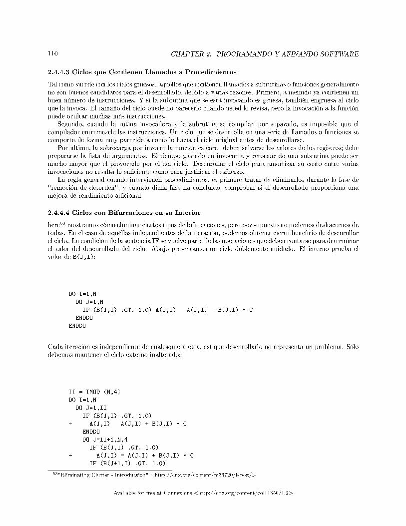
110 CHAPTER 2. PROGRAMANDO Y AFINANDO SOFTWARE
2.4.4.3 Ciclos que Contienen Llamados a Procedimientos
Tal como sucede con los ciclos gruesos, aquellos que contienen llamados a subrutinas o funciones generalmenteno son buenos candidatos para el desenrollado, debido a varias razones. Primero, a menudo ya contienen unbuen número de instrucciones. Y si la subrutina que se está invocando es gruesa, también engruesa al cicloque la invoca. El tamaño del ciclo puede no parecerlo cuando usted lo revisa, pero la invocación a la funciónpuede ocultar muchas más instrucciones.
Segundo, cuando la rutina invocadora y la subrutina se compilan por separado, es imposible que elcompilador entremezcle las instrucciones. Un ciclo que se desenrolla en una serie de llamados a funciones secomporta de forma muy parecida a como lo hacía el ciclo original antes de desenrollarse.
Por último, la sobrecarga por invocar la función es cara: deben salvarse los valores de los registros; debeprepararse la lista de argumentos. El tiempo gastado en invocar a y retornar de una subrutina puede sermucho mayor que el provocado por el del ciclo. Desenrollar el ciclo para amortizar su costo entre variasinvocaciones no resulta lo su�ciente como para justi�car el esfuerzo.
La regla general cuando intervienen procedimientos, es primero tratar de eliminarlos durante la fase de"remoción de desorden", y cuando dicha fase ha concluido, comprobar si el desenrollado proporciona unamejora de rendimiento adicional.
2.4.4.4 Ciclos con Bifurcaciones en su Interior
here63 mostramos cómo eliminar ciertos tipos de bifurcaciones, pero por supuesto no podemos deshacernos detodas. En el caso de aquéllas independientes de la iteración, podemos obtener cierto bene�cio de desenrollarel ciclo. La condición de la sentencia IF se vuelve parte de las operaciones que deben contarse para determinarel valor del desenrollado del ciclo. Abajo presentamos un ciclo doblemente anidado. El interno prueba elvalor de B(J,I):
DO I=1,N
DO J=1,N
IF (B(J,I) .GT. 1.0) A(J,I) = A(J,I) + B(J,I) * C
ENDDO
ENDDO
Cada iteración es independiente de cualesquiera otra, así que desenrollarlo no representa un problema. Sólodebemos mantener el ciclo externo inalterado:
II = IMOD (N,4)
DO I=1,N
DO J=1,II
IF (B(J,I) .GT. 1.0)
+ A(J,I) = A(J,I) + B(J,I) * C
ENDDO
DO J=II+1,N,4
IF (B(J,I) .GT. 1.0)
+ A(J,I) = A(J,I) + B(J,I) * C
IF (B(J+1,I) .GT. 1.0)
63"Eliminating Clutter - Introduction" <http://cnx.org/content/m33720/latest/>
Available for free at Connexions <http://cnx.org/content/col11356/1.2>
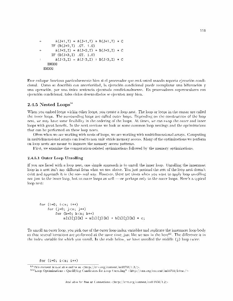
111
+ A(J+1,I) = A(J+1,I) + B(J+1,I) * C
IF (B(J+2,I) .GT. 1.0)
+ A(J+2,I) = A(J+2,I) + B(J+2,I) * C
IF (B(J+3,I) .GT. 1.0)
+ A(J+3,I) = A(J+3,I) + B(J+3,I) * C
ENDDO
ENDDO
Este enfoque funciona particularmente bien si el procesador que está usted usando soporta ejecución condi-cional. Como se describió con anterioridad, la ejecución condicional puede reemplazar una bifurcación yuna operación, por una única sentencia ejecutada condicionalmente. En procesadores superescalares conejecución condicional, tales ciclos desenrollados se ejecutan muy bien.
2.4.5 Nested Loops64
When you embed loops within other loops, you create a loop nest. The loop or loops in the center are calledthe inner loops. The surrounding loops are called outer loops. Depending on the construction of the loopnest, we may have some �exibility in the ordering of the loops. At times, we can swap the outer and innerloops with great bene�t. In the next sections we look at some common loop nestings and the optimizationsthat can be performed on these loop nests.
Often when we are working with nests of loops, we are working with multidimensional arrays. Computingin multidimensional arrays can lead to non-unit-stride memory access. Many of the optimizations we performon loop nests are meant to improve the memory access patterns.
First, we examine the computation-related optimizations followed by the memory optimizations.
2.4.5.1 Outer Loop Unrolling
If you are faced with a loop nest, one simple approach is to unroll the inner loop. Unrolling the innermostloop in a nest isn't any di�erent from what we saw above. You just pretend the rest of the loop nest doesn'texist and approach it in the nor- mal way. However, there are times when you want to apply loop unrollingnot just to the inner loop, but to outer loops as well � or perhaps only to the outer loops. Here's a typicalloop nest:
for (i=0; i<n; i++)
for (j=0; j<n; j++)
for (k=0; k<n; k++)
a[i][j][k] = a[i][j][k] + b[i][j][k] * c;
To unroll an outer loop, you pick one of the outer loop index variables and replicate the innermost loop bodyso that several iterations are performed at the same time, just like we saw in the here65. The di�erence is inthe index variable for which you unroll. In the code below, we have unrolled the middle (j) loop twice:
for (i=0; i<n; i++)
64This content is available online at <http://cnx.org/content/m33734/1.3/>.65"Loop Optimizations - Qualifying Candidates for Loop Unrolling" <http://cnx.org/content/m33733/latest/>
Available for free at Connexions <http://cnx.org/content/col11356/1.2>
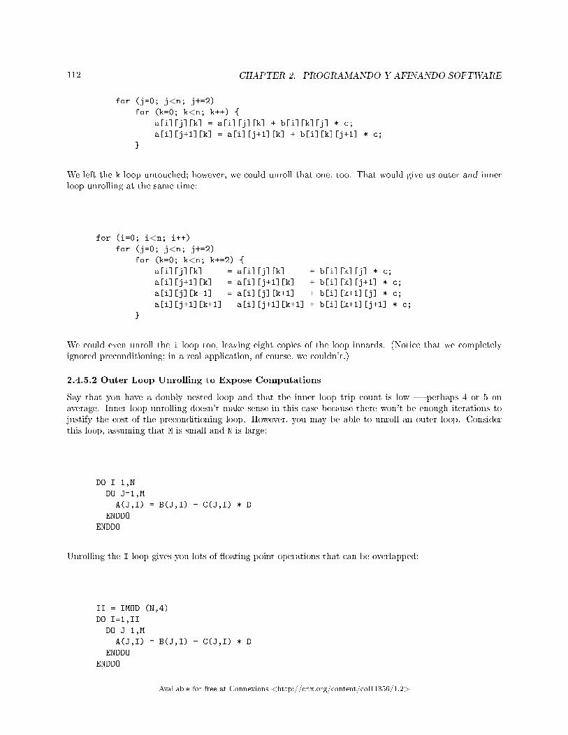
112 CHAPTER 2. PROGRAMANDO Y AFINANDO SOFTWARE
for (j=0; j<n; j+=2)
for (k=0; k<n; k++) {
a[i][j][k] = a[i][j][k] + b[i][k][j] * c;
a[i][j+1][k] = a[i][j+1][k] + b[i][k][j+1] * c;
}
We left the k loop untouched; however, we could unroll that one, too. That would give us outer and innerloop unrolling at the same time:
for (i=0; i<n; i++)
for (j=0; j<n; j+=2)
for (k=0; k<n; k+=2) {
a[i][j][k] = a[i][j][k] + b[i][k][j] * c;
a[i][j+1][k] = a[i][j+1][k] + b[i][k][j+1] * c;
a[i][j][k+1] = a[i][j][k+1] + b[i][k+1][j] * c;
a[i][j+1][k+1] = a[i][j+1][k+1] + b[i][k+1][j+1] * c;
}
We could even unroll the i loop too, leaving eight copies of the loop innards. (Notice that we completelyignored preconditioning; in a real application, of course, we couldn't.)
2.4.5.2 Outer Loop Unrolling to Expose Computations
Say that you have a doubly nested loop and that the inner loop trip count is low � perhaps 4 or 5 onaverage. Inner loop unrolling doesn't make sense in this case because there won't be enough iterations tojustify the cost of the preconditioning loop. However, you may be able to unroll an outer loop. Considerthis loop, assuming that M is small and N is large:
DO I=1,N
DO J=1,M
A(J,I) = B(J,I) + C(J,I) * D
ENDDO
ENDDO
Unrolling the I loop gives you lots of �oating-point operations that can be overlapped:
II = IMOD (N,4)
DO I=1,II
DO J=1,M
A(J,I) = B(J,I) + C(J,I) * D
ENDDO
ENDDO
Available for free at Connexions <http://cnx.org/content/col11356/1.2>
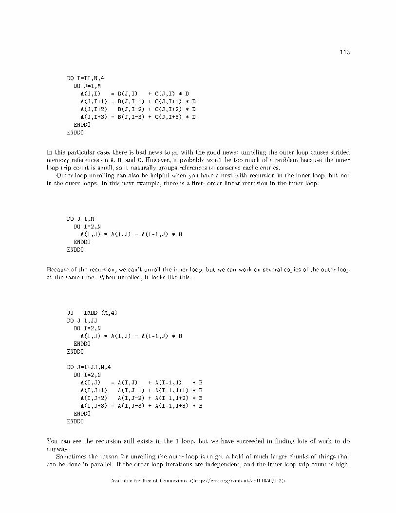
113
DO I=II,N,4
DO J=1,M
A(J,I) = B(J,I) + C(J,I) * D
A(J,I+1) = B(J,I+1) + C(J,I+1) * D
A(J,I+2) = B(J,I+2) + C(J,I+2) * D
A(J,I+3) = B(J,I+3) + C(J,I+3) * D
ENDDO
ENDDO
In this particular case, there is bad news to go with the good news: unrolling the outer loop causes stridedmemory references on A, B, and C. However, it probably won't be too much of a problem because the innerloop trip count is small, so it naturally groups references to conserve cache entries.
Outer loop unrolling can also be helpful when you have a nest with recursion in the inner loop, but notin the outer loops. In this next example, there is a �rst- order linear recursion in the inner loop:
DO J=1,M
DO I=2,N
A(I,J) = A(I,J) + A(I-1,J) * B
ENDDO
ENDDO
Because of the recursion, we can't unroll the inner loop, but we can work on several copies of the outer loopat the same time. When unrolled, it looks like this:
JJ = IMOD (M,4)
DO J=1,JJ
DO I=2,N
A(I,J) = A(I,J) + A(I-1,J) * B
ENDDO
ENDDO
DO J=1+JJ,M,4
DO I=2,N
A(I,J) = A(I,J) + A(I-1,J) * B
A(I,J+1) = A(I,J+1) + A(I-1,J+1) * B
A(I,J+2) = A(I,J+2) + A(I-1,J+2) * B
A(I,J+3) = A(I,J+3) + A(I-1,J+3) * B
ENDDO
ENDDO
You can see the recursion still exists in the I loop, but we have succeeded in �nding lots of work to doanyway.
Sometimes the reason for unrolling the outer loop is to get a hold of much larger chunks of things thatcan be done in parallel. If the outer loop iterations are independent, and the inner loop trip count is high,
Available for free at Connexions <http://cnx.org/content/col11356/1.2>

114 CHAPTER 2. PROGRAMANDO Y AFINANDO SOFTWARE
then each outer loop iteration represents a signi�cant, parallel chunk of work. On a single CPU that doesn'tmatter much, but on a tightly coupled multiprocessor, it can translate into a tremendous increase in speeds.
2.4.6 Loop Interchange66
Loop interchange is a technique for rearranging a loop nest so that the right stu� is at the center. Whatthe right stu� is depends upon what you are trying to accomplish. In many situations, loop interchange alsolets you swap high trip count loops for low trip count loops, so that activity gets pulled into the center ofthe loop nest.67
2.4.6.1 Loop Interchange to Move Computations to the Center
When someone writes a program that represents some kind of real-world model, they often structure thecode in terms of the model. This makes perfect sense. The computer is an analysis tool; you aren't writingthe code on the computer's behalf. However, a model expressed naturally often works on one point in spaceat a time, which tends to give you insigni�cant inner loops � at least in terms of the trip count. Forperformance, you might want to interchange inner and outer loops to pull the activity into the center, whereyou can then do some unrolling. Let's illustrate with an example. Here's a loop where KDIM time-dependentquantities for points in a two-dimensional mesh are being updated:
PARAMETER (IDIM = 1000, JDIM = 1000, KDIM = 3)
...
DO I=1,IDIM
DO J=1,JDIM
DO K=1,KDIM
D(K,J,I) = D(K,J,I) + V(K,J,I) * DT
ENDDO
ENDDO
ENDDO
In practice, KDIM is probably equal to 2 or 3, where J or I, representing the number of points, may be in thethousands. The way it is written, the inner loop has a very low trip count, making it a poor candidate forunrolling.
By interchanging the loops, you update one quantity at a time, across all of the points. For tuningpurposes, this moves larger trip counts into the inner loop and allows you to do some strategic unrolling:
DO K=1,KDIM
DO J=1,JDIM
DO I=1,IDIM
D(K,J,I) = D(K,J,I) + V(K,J,I) * DT
ENDDO
ENDDO
ENDDO
66This content is available online at <http://cnx.org/content/m33736/1.3/>.67It's also good for improving memory access patterns.
Available for free at Connexions <http://cnx.org/content/col11356/1.2>
115
This example is straightforward; it's easy to see that there are no inter-iteration dependencies. But howcan you tell, in general, when two loops can be inter- changed? Interchanging loops might violate somedependency, or worse, only violate it occasionally, meaning you might not catch it when optimizing. Can weinterchange the loops below?
DO I=1,N-1
DO J=2,N
A(I,J) = A(I+1,J-1) * B(I,J)
C(I,J) = B(J,I)
ENDDO
ENDDO
While it is possible to examine the loops by hand and determine the dependencies, it is much better ifthe compiler can make the determination. Very few single-processor compilers automatically perform loopinterchange. However, the compilers for high-end vector and parallel computers generally interchange loopsif there is some bene�t and if interchanging the loops won't alter the program results.68
2.4.7 Memory Access Patterns69
The best pattern is the most straightforward: increasing and unit sequential. For an array with a singledimension, stepping through one element at a time will accomplish this. For multiply-dimensioned arrays,access is fastest if you iterate on the array subscript o�ering the smallest stride or step size. In FORTRANprograms, this is the leftmost subscript; in C, it is the rightmost. The FORTRAN loop below has unit stride,and therefore will run quickly:
DO J=1,N
DO I=1,N
A(I,J) = B(I,J) + C(I,J) * D
ENDDO
ENDDO
In contrast, the next loop is slower because its stride is N (which, we assume, is greater than 1). As Nincreases from one to the length of the cache line (adjusting for the length of each element), the performanceworsens. Once N is longer than the length of the cache line (again adjusted for element size), the performancewon't decrease:
DO J=1,N
DO I=1,N
A(J,I) = B(J,I) + C(J,I) * D
68When the compiler performs automatic parallel optimization, it prefers to run the outermost loop in parallel to minimizeoverhead and unroll the innermost loop to make best use of a superscalar or vector processor. For this reason, the compilerneeds to have some �exibility in ordering the loops in a loop nest.
69This content is available online at <http://cnx.org/content/m33738/1.3/>.
Available for free at Connexions <http://cnx.org/content/col11356/1.2>
116 CHAPTER 2. PROGRAMANDO Y AFINANDO SOFTWARE
ENDDO
ENDDO
Here's a unit-stride loop like the previous one, but written in C:
for (i=0; i<n; i++)
for (j=0; j<n; j++)
a[i][j] = a[i][j] + c[i][j] * d;
Unit stride gives you the best performance because it conserves cache entries. Recall how a data cacheworks.70 Your program makes a memory reference; if the data is in the cache, it gets returned immediately.If not, your program su�ers a cache miss while a new cache line is fetched from main memory, replacingan old one. The line holds the values taken from a handful of neighboring memory locations, including theone that caused the cache miss. If you loaded a cache line, took one piece of data from it, and threw therest away, you would be wasting a lot of time and memory bandwidth. However, if you brought a line intothe cache and consumed everything in it, you would bene�t from a large number of memory references for asmall number of cache misses. This is exactly what you get when your program makes unit-stride memoryreferences.
The worst-case patterns are those that jump through memory, especially a large amount of memory, andparticularly those that do so without apparent rhyme or reason (viewed from the outside). On jobs thatoperate on very large data structures, you pay a penalty not only for cache misses, but for TLB misses too.71
It would be nice to be able to rein these jobs in so that they make better use of memory. Of course, youcan't eliminate memory references; programs have to get to their data one way or another. The question is,then: how can we restructure memory access patterns for the best performance?
In the next few sections, we are going to look at some tricks for restructuring loops with strided, albeitpredictable, access patterns. The tricks will be familiar; they are mostly loop optimizations from here72, usedhere for di�erent reasons. The underlying goal is to minimize cache and TLB misses as much as possible.You will see that we can do quite a lot, although some of this is going to be ugly.
2.4.7.1 Loop Interchange to Ease Memory Access Patterns
Loop interchange is a good technique for lessening the impact of strided memory references. Let's revisitour FORTRAN loop with non-unit stride. The good news is that we can easily interchange the loops; eachiteration is independent of every other:
DO J=1,N
DO I=1,N
A(J,I) = B(J,I) + C(J,I) * D
ENDDO
ENDDO
70See (<http://cnx.org/content/m32733/latest/>).71The Translation Lookaside Bu�er (TLB) is a cache of translations from virtual memory addresses to physical memory
addresses. For more information, refer back to (<http://cnx.org/content/m32733/latest/>).72"Eliminating Clutter - Introduction" <http://cnx.org/content/m33720/latest/>
Available for free at Connexions <http://cnx.org/content/col11356/1.2>
117
After interchange, A, B, and C are referenced with the leftmost subscript varying most quickly. This modi�-cation can make an important di�erence in performance. We traded three N-strided memory references forunit strides:
DO I=1,N
DO J=1,N
A(J,I) = B(J,I) + C(J,I) * D
ENDDO
ENDDO
2.4.7.2 Matrix Multiplication
Matrix multiplication is a common operation we can use to explore the options that are available in optimizinga loop nest. A programmer who has just �nished reading a linear algebra textbook would probably writematrix multiply as it appears in the example below:
DO I=1,N
DO J=1,N
SUM = 0
DO K=1,N
SUM = SUM + A(I,K) * B(K,J)
ENDDO
C(I,J) = SUM
ENDDO
ENDDO
The problem with this loop is that the A(I,K) will be non-unit stride. Each iteration in the inner loopconsists of two loads (one non-unit stride), a multiplication, and an addition.
Given the nature of the matrix multiplication, it might appear that you can't eliminate the non-unitstride. However, with a simple rewrite of the loops all the memory accesses can be made unit stride:
DO J=1,N
DO I=1,N
C(I,J) = 0.0
ENDDO
ENDDO
DO K=1,N
DO J=1,N
SCALE = B(K,J)
DO I=1,N
C(I,J) = C(I,J) + A(I,K) * SCALE
Available for free at Connexions <http://cnx.org/content/col11356/1.2>
118 CHAPTER 2. PROGRAMANDO Y AFINANDO SOFTWARE
ENDDO
ENDDO
ENDDO
Now, the inner loop accesses memory using unit stride. Each iteration performs two loads, one store, amultiplication, and an addition. When comparing this to the previous loop, the non-unit stride loads havebeen eliminated, but there is an additional store operation. Assuming that we are operating on a cache-basedsystem, and the matrix is larger than the cache, this extra store won't add much to the execution time. Thestore is to the location in C(I,J) that was used in the load. In most cases, the store is to a line that isalready in the in the cache. The B(K,J) becomes a constant scaling factor within the inner loop.
2.4.8 When Interchange Won't Work73
In the matrix multiplication code, we encountered a non-unit stride and were able to eliminate it with aquick interchange of the loops. Unfortunately, life is rarely this simple. Often you �nd some mix of variableswith unit and non-unit strides, in which case interchanging the loops moves the damage around, but doesn'tmake it go away.
The loop to perform a matrix transpose represents a simple example of this dilemma:
DO I=1,N DO 20 J=1,M
DO J=1,M DO 10 I=1,N
A(J,I) = B(I,J) A(J,I) = B(I,J)
ENDDO ENDDO
ENDDO ENDDO
Whichever way you interchange them, you will break the memory access pattern for either A or B. Evenmore interesting, you have to make a choice between strided loads vs. strided stores: which will it be?74
We really need a general method for improving the memory access patterns for bothA and B, not one or theother. We'll show you such a method in Section 2.4.9.
2.4.9 Blocking to Ease Memory Access Patterns75
Blocking is another kind of memory reference optimization. As with loop interchange, the challenge is toretrieve as much data as possible with as few cache misses as possible. We'd like to rearrange the loop nestso that it works on data in little neighborhoods, rather than striding through memory like a man on stilts.Given the following vector sum, how can we rearrange the loop?
DO I=1,N
DO J=1,N
A(J,I) = A(J,I) + B(I,J)
ENDDO
73This content is available online at <http://cnx.org/content/m33741/1.3/>.74I can't tell you which is the better way to cast it; it depends on the brand of computer. Some perform better with the
loops left as they are, sometimes by more than a factor of two. Others perform better with them interchanged. The di�erenceis in the way the processor handles updates of main memory from cache.
75This content is available online at <http://cnx.org/content/m33756/1.3/>.
Available for free at Connexions <http://cnx.org/content/col11356/1.2>
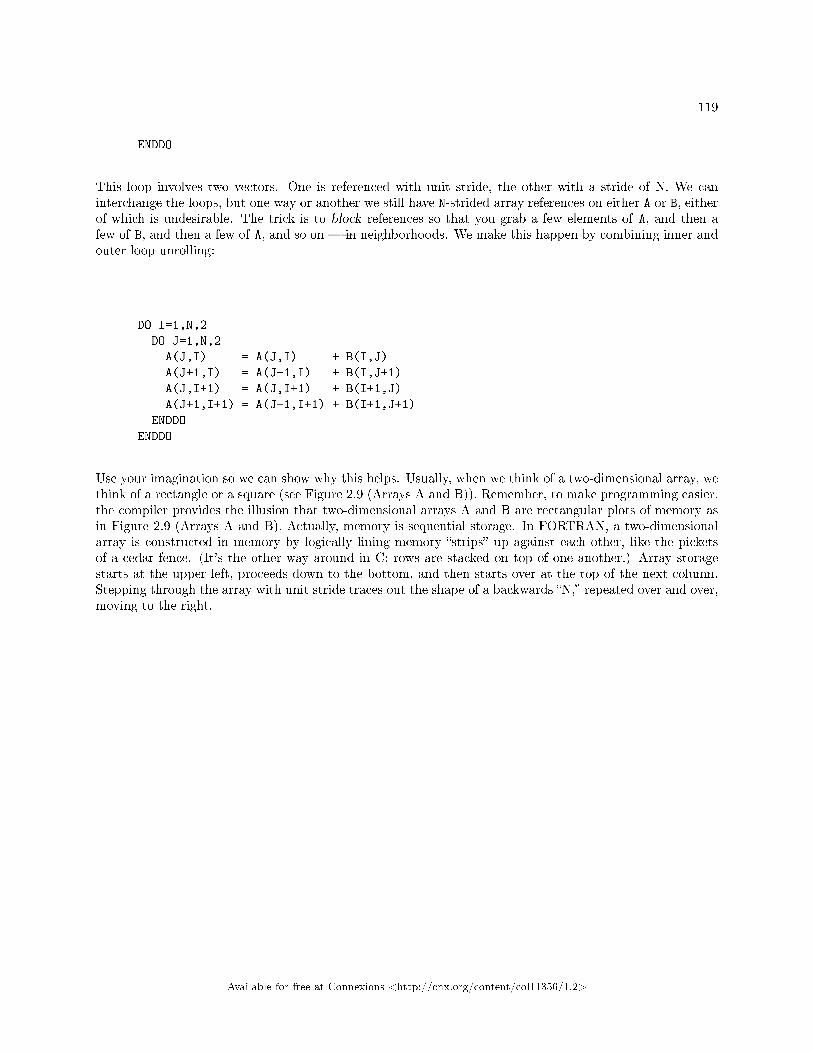
119
ENDDO
This loop involves two vectors. One is referenced with unit stride, the other with a stride of N. We caninterchange the loops, but one way or another we still have N-strided array references on either A or B, eitherof which is undesirable. The trick is to block references so that you grab a few elements of A, and then afew of B, and then a few of A, and so on � in neighborhoods. We make this happen by combining inner andouter loop unrolling:
DO I=1,N,2
DO J=1,N,2
A(J,I) = A(J,I) + B(I,J)
A(J+1,I) = A(J+1,I) + B(I,J+1)
A(J,I+1) = A(J,I+1) + B(I+1,J)
A(J+1,I+1) = A(J+1,I+1) + B(I+1,J+1)
ENDDO
ENDDO
Use your imagination so we can show why this helps. Usually, when we think of a two-dimensional array, wethink of a rectangle or a square (see Figure 2.9 (Arrays A and B)). Remember, to make programming easier,the compiler provides the illusion that two-dimensional arrays A and B are rectangular plots of memory asin Figure 2.9 (Arrays A and B). Actually, memory is sequential storage. In FORTRAN, a two-dimensionalarray is constructed in memory by logically lining memory �strips� up against each other, like the picketsof a cedar fence. (It's the other way around in C: rows are stacked on top of one another.) Array storagestarts at the upper left, proceeds down to the bottom, and then starts over at the top of the next column.Stepping through the array with unit stride traces out the shape of a backwards �N,� repeated over and over,moving to the right.
Available for free at Connexions <http://cnx.org/content/col11356/1.2>
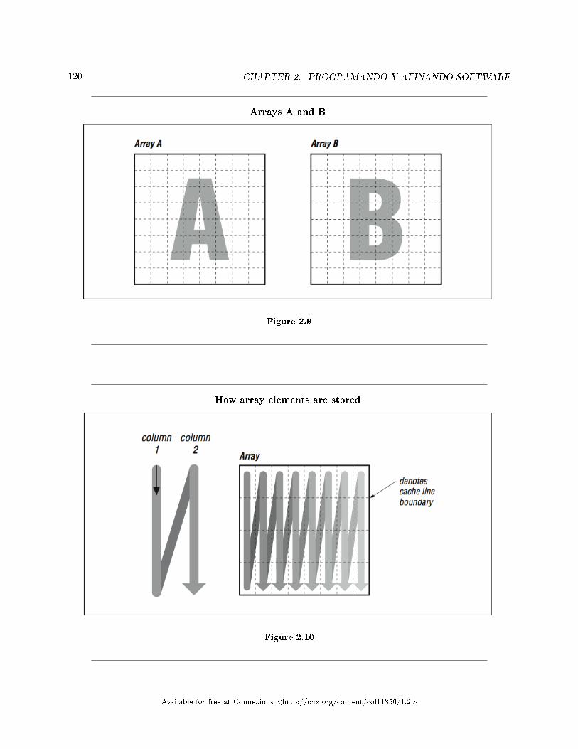
120 CHAPTER 2. PROGRAMANDO Y AFINANDO SOFTWARE
Arrays A and B
Figure 2.9
How array elements are stored
Figure 2.10
Available for free at Connexions <http://cnx.org/content/col11356/1.2>
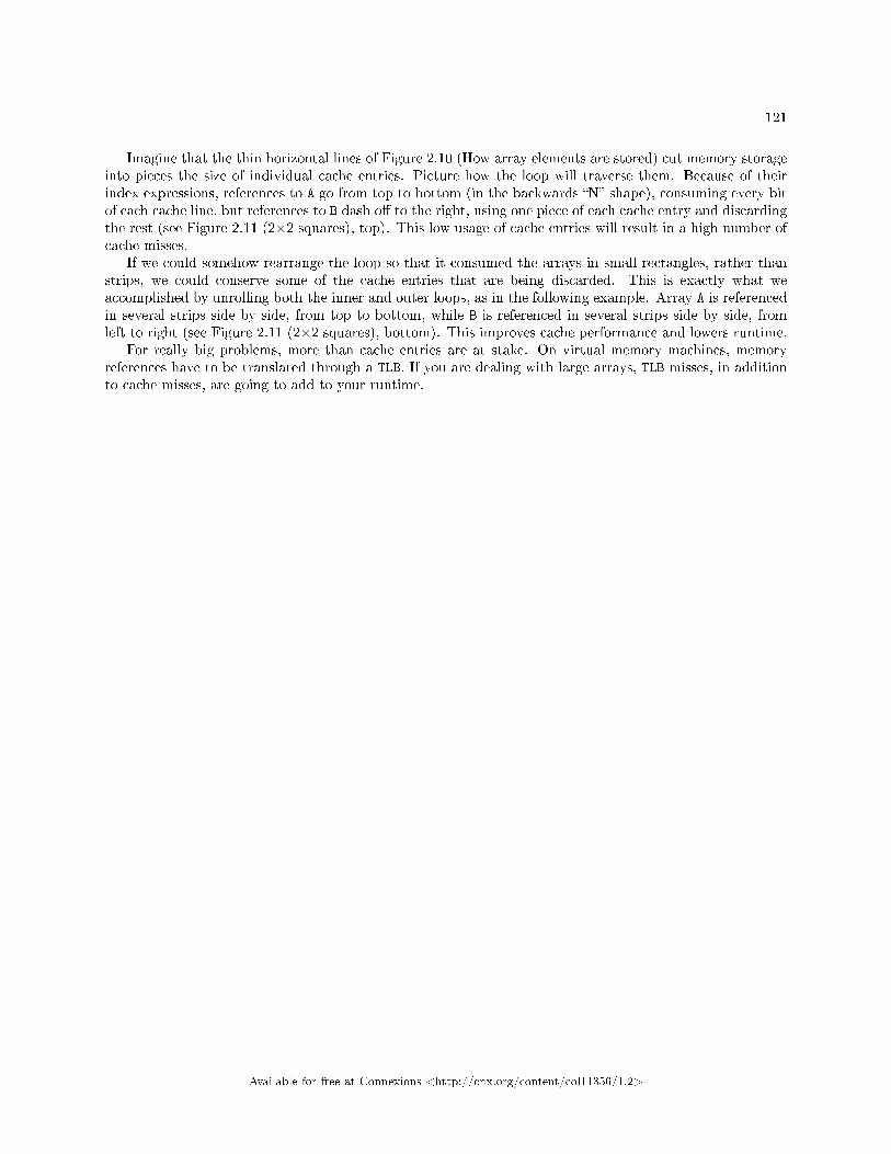
121
Imagine that the thin horizontal lines of Figure 2.10 (How array elements are stored) cut memory storageinto pieces the size of individual cache entries. Picture how the loop will traverse them. Because of theirindex expressions, references to A go from top to bottom (in the backwards �N� shape), consuming every bitof each cache line, but references to B dash o� to the right, using one piece of each cache entry and discardingthe rest (see Figure 2.11 (2×2 squares), top). This low usage of cache entries will result in a high number ofcache misses.
If we could somehow rearrange the loop so that it consumed the arrays in small rectangles, rather thanstrips, we could conserve some of the cache entries that are being discarded. This is exactly what weaccomplished by unrolling both the inner and outer loops, as in the following example. Array A is referencedin several strips side by side, from top to bottom, while B is referenced in several strips side by side, fromleft to right (see Figure 2.11 (2×2 squares), bottom). This improves cache performance and lowers runtime.
For really big problems, more than cache entries are at stake. On virtual memory machines, memoryreferences have to be translated through a TLB. If you are dealing with large arrays, TLB misses, in additionto cache misses, are going to add to your runtime.
Available for free at Connexions <http://cnx.org/content/col11356/1.2>
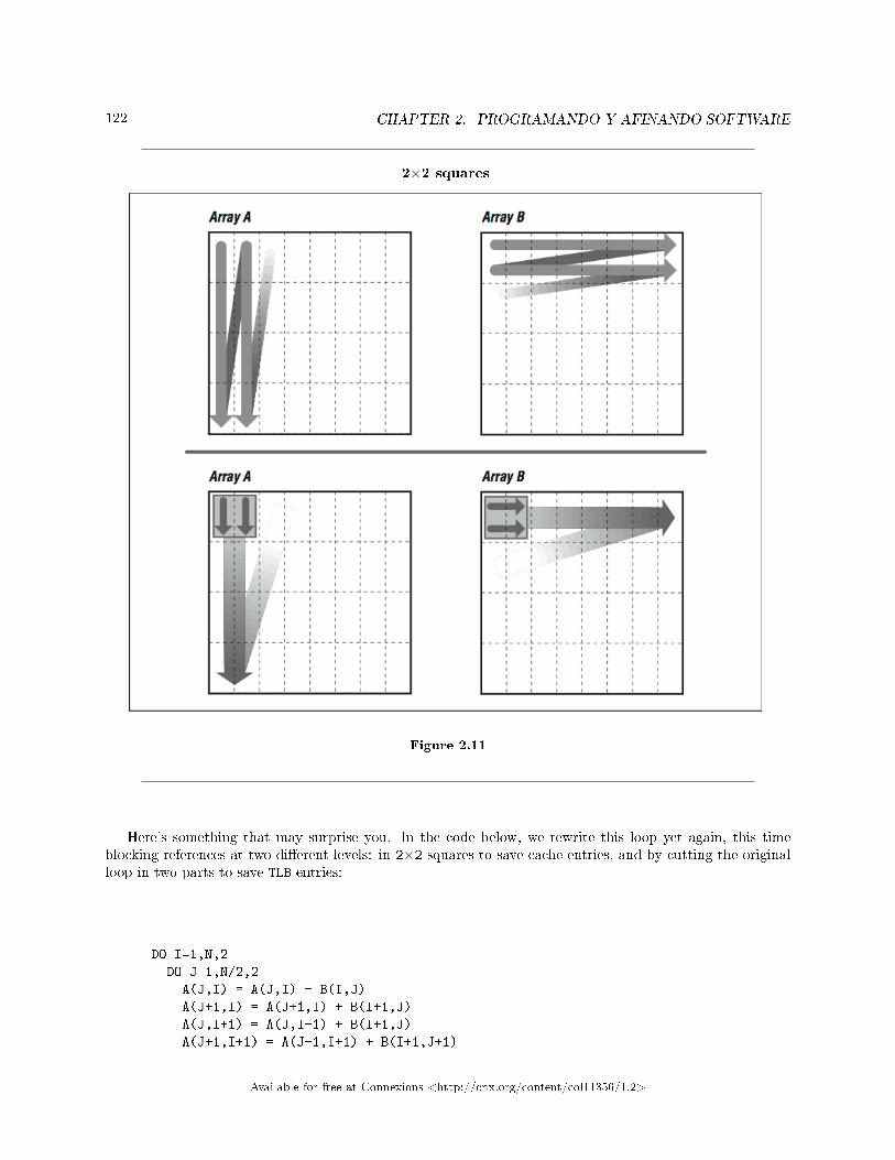
122 CHAPTER 2. PROGRAMANDO Y AFINANDO SOFTWARE
2×2 squares
Figure 2.11
Here's something that may surprise you. In the code below, we rewrite this loop yet again, this timeblocking references at two di�erent levels: in 2×2 squares to save cache entries, and by cutting the originalloop in two parts to save TLB entries:
DO I=1,N,2
DO J=1,N/2,2
A(J,I) = A(J,I) + B(I,J)
A(J+1,I) = A(J+1,I) + B(I+1,J)
A(J,I+1) = A(J,I+1) + B(I+1,J)
A(J+1,I+1) = A(J+1,I+1) + B(I+1,J+1)
Available for free at Connexions <http://cnx.org/content/col11356/1.2>

123
ENDDO
ENDDO
DO I=1,N,2
DO J=N/2+1,N,2
A(J,I) = A(J,I) + B(I,J)
A(J+1,I) = A(J+1,I) + B(I+1,J)
A(J,I+1) = A(J,I+1) + B(I+1,J)
A(J+1,I+1) = A(J+1,I+1) + B(I+1,J+1)
ENDDO
ENDDO
You might guess that adding more loops would be the wrong thing to do. But if you work with a reasonablylarge value of N, say 512, you will see a signi�cant increase in performance. This is because the two arraysA and B are each 256 KB × 8 bytes = 2 MB when N is equal to 512 � larger than can be handled by theTLBs and caches of most processors.
The two boxes in Figure 2.12 (Picture of unblocked versus blocked references) illustrate how the �rst fewreferences to A and B look superimposed upon one another in the blocked and unblocked cases. Unblockedreferences to B zing o� through memory, eating through cache and TLB entries. Blocked references are moresparing with the memory system.
Picture of unblocked versus blocked references
Figure 2.12
You can take blocking even further for larger problems. This code shows another method that limits thesize of the inner loop and visits it repeatedly:
Available for free at Connexions <http://cnx.org/content/col11356/1.2>
124 CHAPTER 2. PROGRAMANDO Y AFINANDO SOFTWARE
II = MOD (N,16)
JJ = MOD (N,4)
DO I=1,N
DO J=1,JJ
A(J,I) = A(J,I) + B(J,I)
ENDDO
ENDDO
DO I=1,II
DO J=JJ+1,N
A(J,I) = A(J,I) + B(J,I)
A(J,I) = A(J,I) + 1.0D0
ENDDO
ENDDO
DO I=II+1,N,16
DO J=JJ+1,N,4
DO K=I,I+15
A(J,K) = A(J,K) + B(K,J)
A(J+1,K) = A(J+1,K) + B(K,J+1)
A(J+2,K) = A(J+2,K) + B(K,J+2)
A(J+3,K) = A(J+3,K) + B(K,J+3)
ENDDO
ENDDO
ENDDO
Where the inner I loop used to execute N iterations at a time, the new K loop executes only 16 iterations.This divides and conquers a large memory address space by cutting it into little pieces.
While these blocking techniques begin to have diminishing returns on single-processor systems, on largemultiprocessor systems with nonuniform memory access (NUMA), there can be signi�cant bene�t in carefullyarranging memory accesses to maximize reuse of both cache lines and main memory pages.
Again, the combined unrolling and blocking techniques we just showed you are for loops with mixedstride expressions. They work very well for loop nests like the one we have been looking at. However, if allarray references are strided the same way, you will want to try loop unrolling or loop interchange �rst.
2.4.10 Programs That Require More Memory Than You Have76
People occasionally have programs whose memory size requirements are so great that the data can't �t inmemory all at once. At any time, some of the data has to reside outside of main memory on secondary(usually disk) storage. These out-of- core solutions fall into two categories:
• Software-managed, out-of-core solutions• Virtual memory�managed, out-of-core solutions
With a software-managed approach, the programmer has recognized that the problem is too big and hasmodi�ed the source code to move sections of the data out to disk for retrieval at a later time. The othermethod depends on the computer's memory system handling the secondary storage requirements on its own,some- times at a great cost in runtime.
76This content is available online at <http://cnx.org/content/m33770/1.3/>.
Available for free at Connexions <http://cnx.org/content/col11356/1.2>
125
2.4.10.1 Software-Managed, Out-of-Core Solutions
Most codes with software-managed, out-of-core solutions have adjustments; you can tell the program howmuch memory it has to work with, and it takes care of the rest. It is important to make sure the adjustmentis set correctly. Code that was tuned for a machine with limited memory could have been ported to anotherwithout taking into account the storage available. Perhaps the whole problem will �t easily.
If we are writing an out-of-core solution, the trick is to group memory references together so that theyare localized. This usually occurs naturally as a side e�ect of partitioning, say, a matrix factorization intogroups of columns. Blocking references the way we did in the previous section also corrals memory referencestogether so you can treat them as memory �pages.� Knowing when to ship them o� to disk entails beingclosely involved with what the program is doing.
2.4.11 Closing Notes77
Loops are the heart of nearly all high performance programs. The �rst goal with loops is to express them assimply and clearly as possible (i.e., eliminates the clutter). Then, use the pro�ling and timing tools to �gureout which routines and loops are taking the time. Once you �nd the loops that are using the most time, tryto determine if the performance of the loops can be improved.
First try simple modi�cations to the loops that don't reduce the clarity of the code. You can alsoexperiment with compiler options that control loop optimizations. Once you've exhausted the options ofkeeping the code looking clean, and if you still need more performance, resort to hand-modifying to thecode. Typically the loops that need a little hand-coaxing are loops that are making bad use of the memoryarchitecture on a cache-based system. Hopefully the loops you end up changing are only a few of the overallloops in the program.
However, before going too far optimizing on a single processor machine, take a look at how the programexecutes on a parallel system. Sometimes the modi�cations that improve performance on a single-processorsystem confuses the parallel-processor compiler. The compilers on parallel and vector systems generally havemore powerful optimization capabilities, as they must identify areas of your code that will execute well ontheir specialized hardware. These compilers have been interchanging and unrolling loops automatically forsome time now.
2.4.12 Exercises78
Exercise 2.4.12.1Why is an unrolling amount of three or four iterations generally su�cient for simple vector loopson a RISC processor? What relationship does the unrolling amount have to �oating-point pipelinedepths?
Exercise 2.4.12.2On a processor that can execute one �oating-point multiply, one �oating-point addi-
tion/subtraction, and one memory reference per cycle, what's the best performance you couldexpect from the following loop?
DO I = 1,10000
A(I) = B(I) * C(I) - D(I) * E(I)
ENDDO
77This content is available online at <http://cnx.org/content/m33773/1.3/>.78This content is available online at <http://cnx.org/content/m33777/1.3/>.
Available for free at Connexions <http://cnx.org/content/col11356/1.2>
126 CHAPTER 2. PROGRAMANDO Y AFINANDO SOFTWARE
Exercise 2.4.12.3Try unrolling, interchanging, or blocking the loop in subroutine BAZFAZ to increase the performance.What method or combination of methods works best? Look at the assembly language created bythe compiler to see what its approach is at the highest level of optimization.
note: Compile the main routine and BAZFAZ separately; adjust NTIMES so that the untuned runtakes about one minute; and use the compiler's default optimization level.
PROGRAM MAIN
IMPLICIT NONE
INTEGER M,N,I,J
PARAMETER (N = 512, M = 640, NTIMES = 500)
DOUBLE PRECISION Q(N,M), R(M,N)
C
DO I=1,M
DO J=1,N
Q(J,I) = 1.0D0
R(I,J) = 1.0D0
ENDDO
ENDDO
C
DO I=1,NTIMES
CALL BAZFAZ (Q,R,N,M)
ENDDO
END
SUBROUTINE BAZFAZ (Q,R,N,M)
IMPLICIT NONE
INTEGER M,N,I,J
DOUBLE PRECISION Q(N,M), R(N,M)
C
DO I=1,N
DO J=1,M
R(I,J) = Q(I,J) * R(J,I)
ENDDO
ENDDO
C
END
Exercise 2.4.12.4Code the matrix multiplication algorithm in the �straightforward� manner and compile it withvarious optimization levels. See if the compiler performs any type of loop interchange.
Try the same experiment with the following code:
DO I=1,N
Available for free at Connexions <http://cnx.org/content/col11356/1.2>
127
DO J=1,N
A(I,J) = A(I,J) + 1.3
ENDDO
ENDDO
Do you see a di�erence in the compiler's ability to optimize these two loops? If you see a di�erence,explain it.
Exercise 2.4.12.5Code the matrix multiplication algorithm both the ways shown in this chapter. Execute theprogram for a range of values for N. Graph the execution time divided by N3 for values of Nranging from 50×50 to 500×500. Explain the performance you see.
Available for free at Connexions <http://cnx.org/content/col11356/1.2>

128 CHAPTER 2. PROGRAMANDO Y AFINANDO SOFTWARE
Available for free at Connexions <http://cnx.org/content/col11356/1.2>
Chapter 3
Procesadores Paralelos de Memoria
Compartida
3.1 Entendiendo el Paralelismo
3.1.1 Entendiendo el Paralelismo - Introducción1
En cierto sentido, hemos estado hablando acerca de paralelismo desde el inicio del libro. Sólo que en vezde llamarlo "paralelismo", hemos usado términos como "entubamiento", "superescalar" y "�exibilidad delcompilador". Conforme nos adentramos en la programación de multiprocesadores, debemos incrementarnuestro entendimiento del paralelismo, para poder comprender cómo programar estos sistemas de formaefectiva. En corto, mientras obtenemos más recursos paralelos, necesitamos encontrar más paralelismo ennuestro código.
Cuando hablamos de paralelismo, necesitamos entender el concepto de granularidad. La granularidad delparalelismo indica el tamaño de los cálculos que se están realizando simultáneamente entre sincronizaciones.Algunos ejemplos de paralelismo, ordenados de acuerdo al tamaño de grano, son:
• Cuando realiza una suma de enteros de 32 bits, usando un sumador con acarreo por desplazamiento,puede usted sumar parcialmente los bits 0 y 1 al mismo tiempo que los bits 2 y 3.
• En un procesador con entubamiento, mientras se decodi�ca una instrucción, puede recuperarse de lamemoria la siguiente.
• En un procesador escalar de dos vías puede ejecutarse, en un solo ciclo, cualquier combinación de unainstrucción entera y de punto �otante.
• En un multiprocesador, puede usted dividir las iteraciones de un ciclo entre los cuatro procesadoresdel sistema.
• Puede usted dividir un arreglo grande entre cuatro estaciones de trabajo conectadas en red. Cadaestación puede operar sobre su propia información local, y luego intercambiar los valores de fronteraal �nal de cada paso de tiempo.
En este capítulo, comenzamos con el paralelismo a nivel de instrucciones (entubamiento y supesescalar) yavanzamos hacia el paralelismo a nivel de hilos de ejecución, que es el que necesitamos para los sistemasmultiprocesador. Es importante señalar que estos niveles distintos de paralelismo generalmente no entranen con�icto. Incrementar el paralelismo a nivel de hilos en problemas de grano grueso, a menudo hace quesalga a �ote el paralelismo de grano más �no.
El siguiente ciclo está lleno de paralelismo:
1This content is available online at <http://cnx.org/content/m37327/1.1/>.
Available for free at Connexions <http://cnx.org/content/col11356/1.2>
129

130 CHAPTER 3. PROCESADORES PARALELOS DE MEMORIA COMPARTIDA
DO I=1,16000
A(I) = B(I) * 3.14159
ENDDO
Hemos expresado el ciclo en una forma que parece implicar que debe calcularse A(1) primero, seguido porA(2), y así sucesivamente. Sin embargo, una vez completado el ciclo, no tiene importancia si A(16000) secalculó antes o después que A(15999). Bien pudiera haberse calculado primero todos los valores pares deI y luego los nones. Tampoco hubiera hecho una diferencia si las 16,000 iteraciones se hubieran calculadosimultáneamente, usando un procesador superescalar de 16,000 vías.2 Si el compilador es �exible en cuanto alorden en que ejecuta las instrucciones que componen el programa, puede realizar todas estas simultáneamentesiempre que haya disponible hardware paralelo.
Una técnica usada por los cientí�cos computacionales para analizar formalmente el paralelismo potencialde un algoritmo, consiste en caracterizar cuan rápidamente se ejecutaría con un procesador superescalar de"in�nito número de vías".
No todos los ciclos contienen tanto paralelismo como este sencillo que analizamos. Necesitamos identi�caraquellas cosas que limitan el paralelismo en nuestro código, y quitarlas siempre que sea posible. En capítulosprevios hemos identi�cado y retirado el desorden y reescrito los ciclos para simpli�carlos.
Este capítulo también proporciona here3, en muchas formas. Revisaremos la mecánica de la compilaciónde código, la cuál se aplica aquí, pero no daremos respuesta a todos los "porqués". Las técnicas básicasde análisis de bloques forman la base del trabajo que realiza el compilador cuando trata de lograr mayorparalelismo. Al observar dos piezas de datos, instrucciones, o datos e instrucciones, un compilador deberesponder la pregunta: "¾dependen las unas de las otras?" Existen tres respuesta posibles: sí, no, y no losabemos. La tercera respuesta es, en la práctica, la misma que sí, porque el compilador debe comportarseconservadoramente cuando no puede garantizar que sea seguro reordenar las instrucciones.
Ayudar al compilador a reconocer el paralelismo es uno de los enfoques básicos que toman los especial-istas para a�nar el código. Una ligera reescritura de un ciclo, o cierta información suplementaria dada alcompilador, pueden convertir una respuesta de "no sabemos" en una oportunidad de lograr paralelismo. Esseguro que hay otras facetas en este proceso de a�nación, tales como optimizar los patrones de acceso amemoria de forma que se adapten mejor al hardware, o reelaborar un algoritmo. Y no existe una sola formacorrecta de hacerlo para todos los problemas; cualquier esfuerzo de mejora debe involucrar una combinaciónde técnicas.
3.1.2 Entendiendo el Paralelismo - Dependencias4
Imagine una orquesta sinfónica donde cada músico toque sin tomar en cuenta al director o a lo otros músicos.Al primer movimiento de la batuta del director, cada músico recorre toda su partitura. Algunos �nalizanmucho antes que otros, dejan el escenario y se van a casa. La cacofonía resultante no parece música (pensán-dolo bien, recuerdo algo al jazz experimental), porque carece por completo de coordinación. Por supuesto,esta no es la forma en que se interpreta la música. Un programa de computadora, como una pieza musical, seteje en un telar que lo despliega conforme avanza el tiempo (aunque tal vez lo teje menos compactamente).Ciertas cosas deben suceder antes que otras, y hay una tasa de ejecución para el proceso en su conjunto.
En los programas de computadora, cuando un evento A debe suceder antes de otro evento B, se dice queB es dependiente de A. Llamamos a esta relación entre ellos una dependencia. En ocasiones las dependencias
2Curiosamente, esta idea no es tan descabellada como pareciera. Sobre una computadora SIMD (una sola instrucción,múltiples datos) como la Connection CM-2 con 16,384 procesadores, tomaría tres ciclos de instrucción procesar este ciclocompleto.
3"What a Compiler Does - Introduction" <http://cnx.org/content/m33690/latest/>4This content is available online at <http://cnx.org/content/m37401/1.1/>.
Available for free at Connexions <http://cnx.org/content/col11356/1.2>
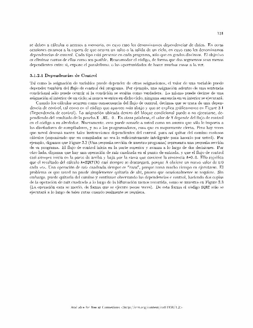
131
se deben a cálculos o accesos a memoria, en cuyo caso les denominamos dependencias de datos. En otrasocasiones estamos a la espera de que ocurra un salto o la salida de un ciclo, en cuyo caso les denominamosdependencias de control. Cada tipo está presente en cada programa, sólo que en grados distintos. El objetivoes eliminar tantas de ellas como sea posible. Reacomodar el código, de forma que dos segmentos sean menosdependientes entre sí, expone el paralelismo, o las oportunidades de hacer muchas cosas a la vez.
3.1.2.1 Dependencias de Control
Tal como la asignación de variables puede depender de otras asignaciones, el valor de una variable puededepender también del �ujo de control del programa. Por ejemplo, una asignación adentro de una sentenciacondicional sólo puede ocurrir si la condición se evalúa como verdadera. Lo mismo puede decirse de unaasignación al interior de un ciclo; si nunca se entra en dicho ciclo, ninguna sentencia en su interior se ejecutará.
Cuando los cálculos ocurren como consecuencia del �ujo de control, decimos que se trata de una depen-dencia de control, tal como en el código que aparece más abajo y que se explica grá�camente en Figure 3.1(Dependencia de control). La asignación ubicada dentro del bloque condicional puede o no ejecutarse, de-pendiendo del resultado de la prueba X .NE. 0. En otras palabras, el valor de Y depende del �ujo de controlen el código a su alrededor. Nuevamente, esto puede sonarle a usted como un asunto que sólo le importa alos diseñadores de compiladores, y no a los programadores, cosa que es mayormente cierta. Pero hay vecesque usted deseará mover tales instrucciones dependientes del control, para así quitar del camino costososcálculos (suponiendo que su compilador no sea lo su�cientemente inteligente para hacerlo por usted). Porejemplo, digamos que Figure 3.2 (Una pequeña sección de nuestro programa) representa una pequeña secciónde su programa. El �ujo de control inicia en la parte superior y avanza a lo largo de dos decisiones. Porotro lado, digamos que hay una operación de raíz cuadrada en el punto de entrada, y que el �ujo de controlcasi siempre inicia en la parte de arriba y baja por la rama que contiene la sentencia A=0.0. Ello signi�caque el resultado del cálculo A=SQRT(B) casi siempre se descargará, porque A obtiene un nuevo valor de 0.0cada vez. Una operación de raíz cuadrada siempre es "cara", porque toma mucho tiempo en ejecutarse. Elproblema es que usted no puede simplemente quitarla de ahí, puesto que ocasionalmente se requiere. Sinembargo, puede quitarla del camino y continuar observando las dependencias e control, haciendo dos copiasde la operación de raíz cuadrada a lo largo de la bifurcación menos recorrida, como se muestra en Figure 3.3(La operación cara se movió, de forma que se ejecute pocas veces). De esta forma el código SQRT sólo seejecutará a lo largo de tales rutas cuando realmente se requiera.
Available for free at Connexions <http://cnx.org/content/col11356/1.2>
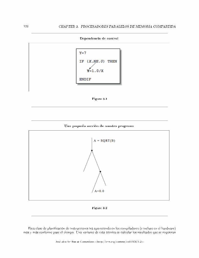
132 CHAPTER 3. PROCESADORES PARALELOS DE MEMORIA COMPARTIDA
Dependencia de control
Figure 3.1
Una pequeña sección de nuestro programa
Figure 3.2
Esta clase de plani�cación de instrucciones irá apareciendo en los compiladores (e incluso en el hardware)más y más conforme pase el tiempo. Una variante de esta técnica es calcular los resultados que se requieran
Available for free at Connexions <http://cnx.org/content/col11356/1.2>
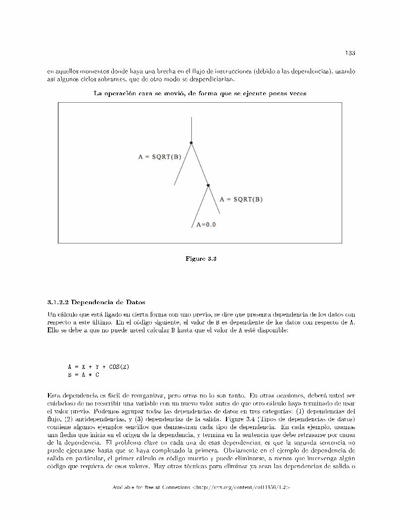
133
en aquellos momentos donde haya una brecha en el �ujo de instrucciones (debido a las dependencias), usandoasí algunos ciclos sobrantes, que de otro modo se desperdiciarían.
La operación cara se movió, de forma que se ejecute pocas veces
Figure 3.3
3.1.2.2 Dependencia de Datos
Un cálculo que está ligado en cierta forma con uno previo, se dice que presenta dependencia de los datos conrespecto a este último. En el código siguiente, el valor de B es dependiente de los datos con respecto de A.Ello se debe a que no puede usted calcular B hasta que el valor de A esté disponible:
A = X + Y + COS(Z)
B = A * C
Esta dependencia es fácil de reorganizar, pero otras no lo son tanto. En otras ocasiones, deberá usted sercuidadoso de no reescribir una variable con un nuevo valor antes de que otro cálculo haya terminado de usarel valor previo. Podemos agrupar todas las dependencias de datos en tres categorías: (1) dependencias del�ujo, (2) antidependencias, y (3) dependencias de la salida. Figure 3.4 (Tipos de dependencias de datos)contiene algunos ejemplos sencillos que demuestran cada tipo de dependencia. En cada ejemplo, usamosuna �echa que inicia en el origen de la dependencia, y termina en la sentencia que debe retrasarse por causade la dependencia. El problema clave en cada una de esas dependencias, es que la segunda sentencia nopuede ejecutarse hasta que se haya completado la primera. Obviamente en el ejemplo de dependencia desalida en particular, el primer cálculo es código muerto y puede eliminarse, a menos que intervenga algúncódigo que requiera de esos valores. Hay otras técnicas para eliminar ya sean las dependencias de salida o
Available for free at Connexions <http://cnx.org/content/col11356/1.2>
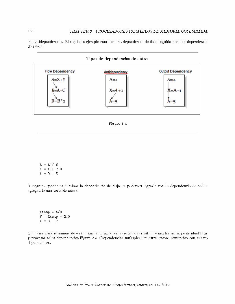
134 CHAPTER 3. PROCESADORES PARALELOS DE MEMORIA COMPARTIDA
las antidependencias. El siguiente ejemplo contiene una dependencia de �ujo seguida por una dependenciade salida:
Tipos de dependencias de datos
Figure 3.4
X = A / B
Y = X + 2.0
X = D - E
Aunque no podamos eliminar la dependencia de �ujo, sí podemos lograrlo con la dependencia de salidaagregando una variable nueva:
Xtemp = A/B
Y = Xtemp + 2.0
X = D - E
Conforme crece el número de sentencias e interacciones entre ellas, necesitamos una forma mejor de identi�cary procesar tales dependencias.Figure 3.5 (Dependencias múltiples) muestra cuatro sentencias con cuatrodependencias.
Available for free at Connexions <http://cnx.org/content/col11356/1.2>
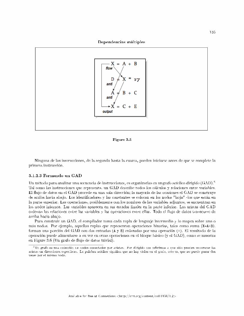
135
Dependencias múltiples
Figure 3.5
Ninguna de las instrucciones, de la segunda hasta la cuarta, pueden iniciarse antes de que se complete laprimera instrucción.
3.1.2.3 Formando un GAD
Un método para analizar una secuencia de instrucciones, es organizarlas en ungrafo acíclico dirigido (GAD).5
Tal como las instrucciones que representa, un GAD describe todos los cálculos y relaciones entre variables.El �ujo de datos en el GAD procede en una sola dirección; la mayoría de las ocasiones el GAD se construyede arriba hacia abajo. Los identi�cadores y las constantes se colocan en los nodos "hoja" -los que están enla parte superior. Las operaciones, posiblemente con los nombres de las variables adjuntos, se encuentran enlos nodos internos. Las variables aparecen en sus estados �nales en la parte inferior. Las aristas del GADordenan las relaciones entre las variables y las operaciones entre ellas. Todo el �ujo de datos transcurre dearriba hacia abajo.
Para construir un GAD, el compilador toma cada tupla de lenguaje intermedio y lo mapea sobre uno omás nodos. Por ejemplo, aquellas tuplas que representan operaciones binarias, tales como suma (X=A+B),forman una porción del GAD con dos entradas (A y B) enlazadas por una operación (+). El resultado de laoperación puede alimentarse a su vez en otras operaciones en el bloque básico (y el GAD), como se muestraen Figure 3.6 (Un grafo de �ujo de datos trivial).
5Un grafo es una colección de nodos conectados por aristas. Por dirigido nos referimos a que sólo pueden recorrerse lasaristas en direcciones especí�cas. La palabra acíclico signi�ca que no hay ciclos en el grafo, esto es, que no puede pasar dosveces por el mismo nodo.
Available for free at Connexions <http://cnx.org/content/col11356/1.2>
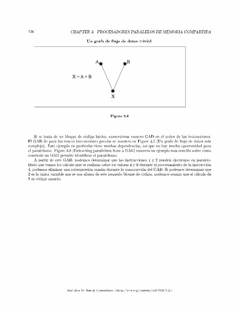
136 CHAPTER 3. PROCESADORES PARALELOS DE MEMORIA COMPARTIDA
Un grafo de �ujo de datos trivial
Figure 3.6
Si se trata de un bloque de código básico, construimos nuestro GAD en el orden de las instrucciones.El GAD de para las cuatro instrucciones previas se muestra en Figure 3.7 (Un grafo de �ujo de datos máscomplejo). Este ejemplo en particular tiene muchas dependencias, así que no hay mucha oportunidad parael paralelismo. Figure 3.8 (Extracting parallelism from a DAG) muestra un ejemplo más sencillo sobre cómoconstruir un GAD permite identi�car el paralelismo.
A partir de este GAD, podemos determinar que las instrucciones 1 y 2 pueden ejecutarse en paralelo.Dado que vemos los cálculo que se realizan sobre los valores A y B durante el procesamiento de la instrucción4, podemos eliminar una subexpresión común durante la construcción del GAD. Si podemos determinar queZ es la única variable que se usa afuera de este pequeño bloque de código, podemos asumir que el cálculo deY es código muerto.
Available for free at Connexions <http://cnx.org/content/col11356/1.2>
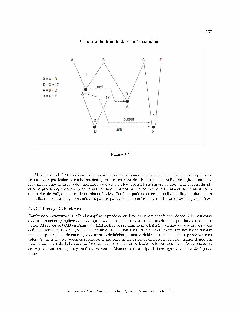
137
Un grafo de �ujo de datos más complejo
Figure 3.7
Al construir el GAD, tomamos una secuencia de instrucciones y determinamos cuáles deben ejecutarseen un orden particular, y cuáles pueden ejecutarse en paralelo. Este tipo de análisis de �ujo de datos esmuy importante en la fase de generación de código en los procesadores superescalares. Hemos introducidoel concepto de dependencias y cómo usar el �ujo de datos para encontrar oportunidades de paralelismo ensecuencias de código adentro de un bloque básico. También podemos usar el análisis de �ujo de datos paraidenti�car dependencias, oportunidades para el paralelismo, y código muerto al interior de bloques básicos.
3.1.2.4 Usos y De�niciones
Conforme se construye el GAD, el compilador puede crear listas de usos y de�niciones de variables, así comootra información, y aplicarlas a las optimizaciones globales a través de muchos bloques básicos tomadosjunto. Al revisar el GAD en Figure 3.8 (Extracting parallelism from a DAG), podemos ver que las variablesde�nidas son Z, Y, X, C, y D, y que las variables usadas son A y B. Al tomar en cuenta muchos bloques comouno solo, podemos decir cuan lejos alcanza la de�nición de una variable particular �dónde puede verse suvalor. A partir de esto podemos reconocer situaciones en las cuales se descartan cálculos, lugares donde dosusos de una variable dada son completamente independientes, o dónde podemos reescribir valores residentesen registros sin tener que regresarlos a memoria. Llamamos a este tipo de investigación análisis de �ujo dedatos.
Available for free at Connexions <http://cnx.org/content/col11356/1.2>
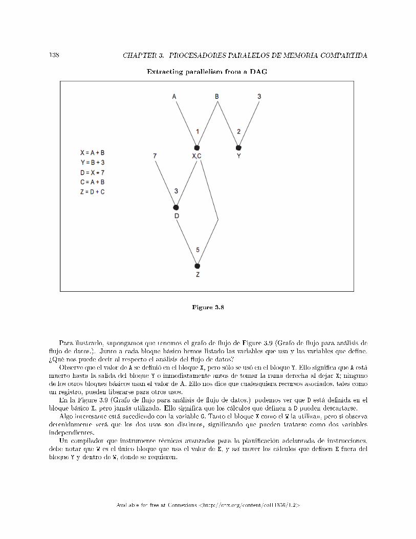
138 CHAPTER 3. PROCESADORES PARALELOS DE MEMORIA COMPARTIDA
Extracting parallelism from a DAG
Figure 3.8
Para ilustrarlo, supongamos que tenemos el grafo de �ujo de Figure 3.9 (Grafo de �ujo para análisis de�ujo de datos.). Junto a cada bloque básico hemos listado las variables que usa y las variables que de�ne.¾Qué nos puede decir al respecto el análisis del �ujo de datos?
Observe que el valor de A se de�nió en el bloque X, pero sólo se usó en el bloque Y. Ello signi�ca que A estámuerto hasta la salida del bloque Y o inmediatamente antes de tomar la rama derecha al dejar X; ningunode los otros bloques básicos usan el valor de A. Ello nos dice que cualesquiera recursos asociados, tales comoun registro, pueden liberarse para otros usos.
En la Figure 3.9 (Grafo de �ujo para análisis de �ujo de datos.) podemos ver que D está de�nida en elbloque básico X, pero jamás utilizada. Ello signi�ca que los cálculos que de�nen a D pueden descartarse.
Algo interesante está sucediendo con la variable G. Tanto el bloque X como el W la utilizan, pero si observadetenidamente verá que los dos usos son distintos, signi�cando que pueden tratarse como dos variablesindependientes.
Un compilador que instrumente técnicas avanzadas para la plani�cación adelantada de instrucciones,debe notar que W es el único bloque que usa el valor de E, y así mover los cálculos que de�nen E fuera delbloque Y y dentro de W, donde se requieren.
Available for free at Connexions <http://cnx.org/content/col11356/1.2>
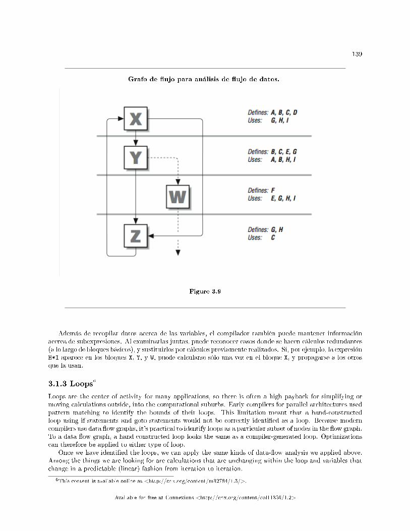
139
Grafo de �ujo para análisis de �ujo de datos.
Figure 3.9
Además de recopilar datos acerca de las variables, el compilador también puede mantener informaciónacerca de subexpresiones. Al examinarlas juntas, puede reconocer casos donde se hacen cálculos redundantes(a lo largo de bloques básicos), y sustituirlos por cálculos previamente realizados. Si, por ejemplo, la expresiónH*I aparece en los bloques X, Y, y W, puede calcularse sólo una vez en el bloque X, y propagarse a los otrosque la usan.
3.1.3 Loops6
Loops are the center of activity for many applications, so there is often a high payback for simplifying ormoving calculations outside, into the computational suburbs. Early compilers for parallel architectures usedpattern matching to identify the bounds of their loops. This limitation meant that a hand-constructedloop using if-statements and goto-statements would not be correctly identi�ed as a loop. Because moderncompilers use data �ow graphs, it's practical to identify loops as a particular subset of nodes in the �ow graph.To a data �ow graph, a hand constructed loop looks the same as a compiler-generated loop. Optimizationscan therefore be applied to either type of loop.
Once we have identi�ed the loops, we can apply the same kinds of data-�ow analysis we applied above.Among the things we are looking for are calculations that are unchanging within the loop and variables thatchange in a predictable (linear) fashion from iteration to iteration.
6This content is available online at <http://cnx.org/content/m32784/1.3/>.
Available for free at Connexions <http://cnx.org/content/col11356/1.2>
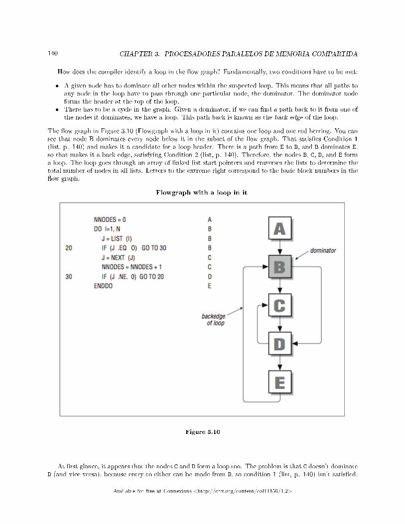
140 CHAPTER 3. PROCESADORES PARALELOS DE MEMORIA COMPARTIDA
How does the compiler identify a loop in the �ow graph? Fundamentally, two conditions have to be met:
• A given node has to dominate all other nodes within the suspected loop. This means that all paths toany node in the loop have to pass through one particular node, the dominator. The dominator nodeforms the header at the top of the loop.
• There has to be a cycle in the graph. Given a dominator, if we can �nd a path back to it from one ofthe nodes it dominates, we have a loop. This path back is known as the back edge of the loop.
The �ow graph in Figure 3.10 (Flowgraph with a loop in it) contains one loop and one red herring. You cansee that node B dominates every node below it in the subset of the �ow graph. That satis�es Condition 1(list, p. 140) and makes it a candidate for a loop header. There is a path from E to B, and B dominates E,so that makes it a back edge, satisfying Condition 2 (list, p. 140). Therefore, the nodes B, C, D, and E forma loop. The loop goes through an array of linked list start pointers and traverses the lists to determine thetotal number of nodes in all lists. Letters to the extreme right correspond to the basic block numbers in the�ow graph.
Flowgraph with a loop in it
Figure 3.10
At �rst glance, it appears that the nodes C and D form a loop too. The problem is that C doesn't dominateD (and vice versa), because entry to either can be made from B, so condition 1 (list, p. 140) isn't satis�ed.
Available for free at Connexions <http://cnx.org/content/col11356/1.2>
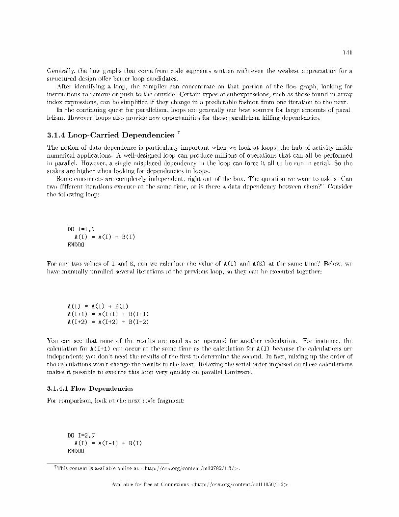
141
Generally, the �ow graphs that come from code segments written with even the weakest appreciation for astructured design o�er better loop candidates.
After identifying a loop, the compiler can concentrate on that portion of the �ow graph, looking forinstructions to remove or push to the outside. Certain types of subexpressions, such as those found in arrayindex expressions, can be simpli�ed if they change in a predictable fashion from one iteration to the next.
In the continuing quest for parallelism, loops are generally our best sources for large amounts of paral-lelism. However, loops also provide new opportunities for those parallelism-killing dependencies.
3.1.4 Loop-Carried Dependencies 7
The notion of data dependence is particularly important when we look at loops, the hub of activity insidenumerical applications. A well-designed loop can produce millions of operations that can all be performedin parallel. However, a single misplaced dependency in the loop can force it all to be run in serial. So thestakes are higher when looking for dependencies in loops.
Some constructs are completely independent, right out of the box. The question we want to ask is �Cantwo di�erent iterations execute at the same time, or is there a data dependency between them?� Considerthe following loop:
DO I=1,N
A(I) = A(I) + B(I)
ENDDO
For any two values of I and K, can we calculate the value of A(I) and A(K) at the same time? Below, wehave manually unrolled several iterations of the previous loop, so they can be executed together:
A(I) = A(I) + B(I)
A(I+1) = A(I+1) + B(I+1)
A(I+2) = A(I+2) + B(I+2)
You can see that none of the results are used as an operand for another calculation. For instance, thecalculation for A(I+1) can occur at the same time as the calculation for A(I) because the calculations areindependent; you don't need the results of the �rst to determine the second. In fact, mixing up the order ofthe calculations won't change the results in the least. Relaxing the serial order imposed on these calculationsmakes it possible to execute this loop very quickly on parallel hardware.
3.1.4.1 Flow Dependencies
For comparison, look at the next code fragment:
DO I=2,N
A(I) = A(I-1) + B(I)
ENDDO
7This content is available online at <http://cnx.org/content/m32782/1.3/>.
Available for free at Connexions <http://cnx.org/content/col11356/1.2>

142 CHAPTER 3. PROCESADORES PARALELOS DE MEMORIA COMPARTIDA
This loop has the regularity of the previous example, but one of the subscripts is changed. Again, it's usefulto manually unroll the loop and look at several iterations together:
A(I) = A(I-1) + B(I)
A(I+1) = A(I) + B(I+1)
A(I+2) = A(I+1) + B(I+2)
In this case, there is a dependency problem. The value of A(I+1) depends on the value of A(I), the value ofA(I+2) depends on A(I+1), and so on; every iteration depends on the result of a previous one. Dependenciesthat extend back to a previous calculation and perhaps a previous iteration (like this one), are loop carried�ow dependencies or backward dependencies. You often see such dependencies in applications that performGaussian elimination on certain types of matrices, or numerical solutions to systems of di�erential equations.However, it is impossible to run such a loop in parallel (as written); the processor must wait for intermediateresults before it can proceed.
In some cases, �ow dependencies are impossible to �x; calculations are so dependent upon one anotherthat we have no choice but to wait for previous ones to complete. Other times, dependencies are a functionof the way the calculations are expressed. For instance, the loop above can be changed to reduce thedependency. By replicating some of the arithmetic, we can make it so that the second and third iterationsdepend on the �rst, but not on one another. The operation count goes up � we have an extra addition thatwe didn't have before � but we have reduced the dependency between iterations:
DO I=2,N,2
A(I) = A(I-1) + B(I)
A(I+1) = A(I-1) + B(I) + B(I+1)
ENDDO
The speed increase on a workstation won't be great (most machines run the recast loop more slowly).However, some parallel computers can trade o� additional calculations for reduced dependency and chalkup a net win.
3.1.4.2 Antidependencies
It's a di�erent story when there is a loop-carried antidependency, as in the code below:
DO I=1,N
A(I) = B(I) * E
B(I) = A(I+2) * C
ENDDO
In this loop, there is an antidependency between the variable A(I) and the variable A(I+2). That is, youmust be sure that the instruction that uses A(I+2) does so before the previous one rede�nes it. Clearly, thisis not a problem if the loop is executed serially, but remember, we are looking for opportunities to overlap
Available for free at Connexions <http://cnx.org/content/col11356/1.2>

143
instructions. Again, it helps to pull the loop apart and look at several iterations together. We have recastthe loop by making many copies of the �rst statement, followed by copies of the second:
A(I) = B(I) * E
A(I+1) = B(I+1) * E
A(I+2) = B(I+2) * E
...
B(I) = A(I+2) * C ← assignment makes use of the new
B(I+1) = A(I+3) * C value of A(I+2) incorrect.
B(I+2) = A(I+4) * C
The reference to A(I+2) needs to access an �old� value, rather than one of the new ones being calculated.If you perform all of the �rst statement followed by all of the second statement, the answers will be wrong.If you perform all of the second statement followed by all of the �rst statement, the answers will also bewrong. In a sense, to run the iterations in parallel, you must either save the A values to use for the secondstatement or store all of the B value in a temporary area until the loop completes.
We can also directly unroll the loop and �nd some parallelism:
1 A(I) = B(I) * E
2 B(I) = A(I+2) * C →3 A(I+1) = B(I+1) * E | Output dependency
4 B(I+1) = A(I+3) * C |
5 A(I+2) = B(I+2) * E ←6 B(I+2) = A(I+4) * C
Statements 1�4 could all be executed simultaneously. Once those statements completed execution, statements5�8 could execute in parallel. Using this approach, there are su�cient intervening statements between thedependent statements that we can see some parallel performance improvement from a superscalar RISCprocessor.
3.1.4.3 Output Dependencies
The third class of data dependencies, output dependencies, is of particular interest to users of parallelcomputers, particularly multiprocessors. Output dependencies involve getting the right values to the rightvariables when all calculations have been completed. Otherwise, an output dependency is violated. The loopbelow assigns new values to two elements of the vector A with each iteration:
DO I=1,N
A(I) = C(I) * 2.
A(I+2) = D(I) + E
ENDDO
Available for free at Connexions <http://cnx.org/content/col11356/1.2>
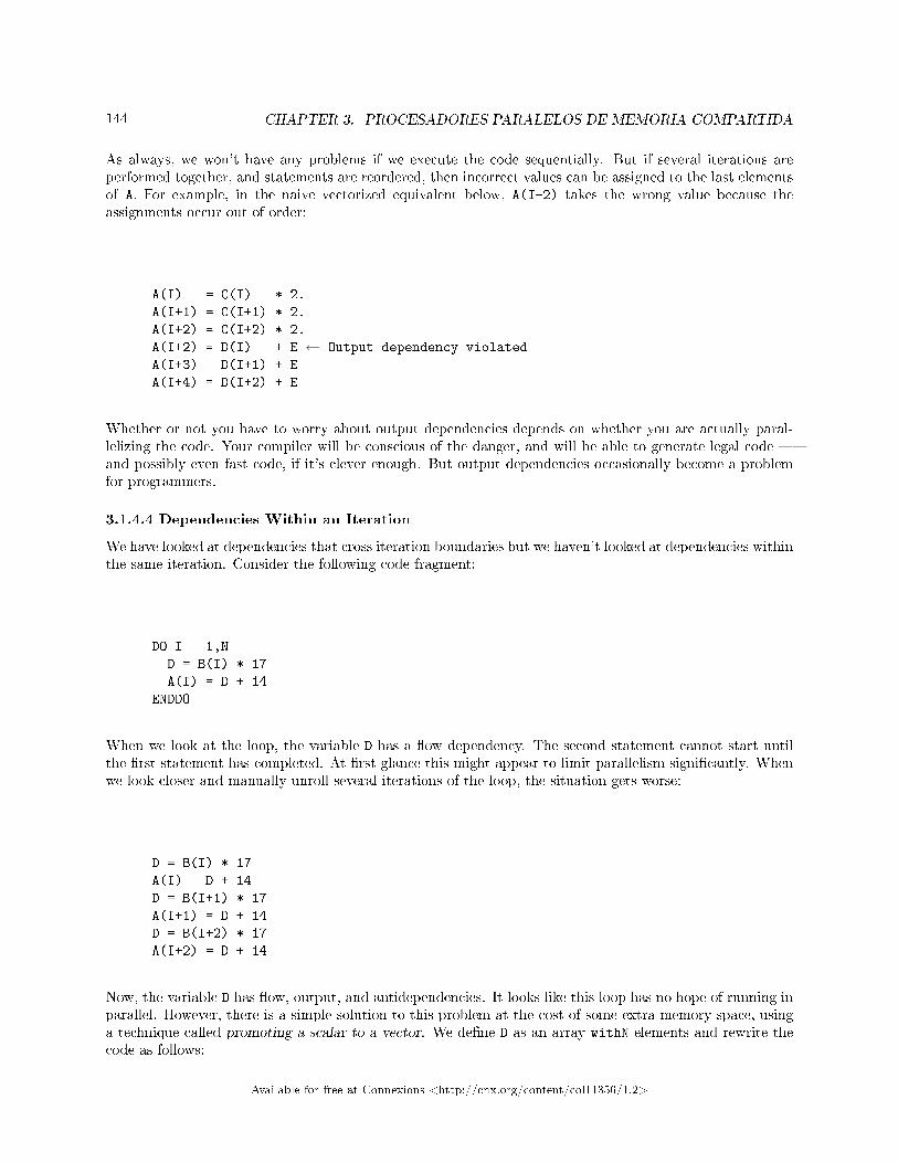
144 CHAPTER 3. PROCESADORES PARALELOS DE MEMORIA COMPARTIDA
As always, we won't have any problems if we execute the code sequentially. But if several iterations areperformed together, and statements are reordered, then incorrect values can be assigned to the last elementsof A. For example, in the naive vectorized equivalent below, A(I+2) takes the wrong value because theassignments occur out of order:
A(I) = C(I) * 2.
A(I+1) = C(I+1) * 2.
A(I+2) = C(I+2) * 2.
A(I+2) = D(I) + E ← Output dependency violated
A(I+3) = D(I+1) + E
A(I+4) = D(I+2) + E
Whether or not you have to worry about output dependencies depends on whether you are actually paral-lelizing the code. Your compiler will be conscious of the danger, and will be able to generate legal code �and possibly even fast code, if it's clever enough. But output dependencies occasionally become a problemfor programmers.
3.1.4.4 Dependencies Within an Iteration
We have looked at dependencies that cross iteration boundaries but we haven't looked at dependencies withinthe same iteration. Consider the following code fragment:
DO I = 1,N
D = B(I) * 17
A(I) = D + 14
ENDDO
When we look at the loop, the variable D has a �ow dependency. The second statement cannot start untilthe �rst statement has completed. At �rst glance this might appear to limit parallelism signi�cantly. Whenwe look closer and manually unroll several iterations of the loop, the situation gets worse:
D = B(I) * 17
A(I) = D + 14
D = B(I+1) * 17
A(I+1) = D + 14
D = B(I+2) * 17
A(I+2) = D + 14
Now, the variable D has �ow, output, and antidependencies. It looks like this loop has no hope of running inparallel. However, there is a simple solution to this problem at the cost of some extra memory space, usinga technique called promoting a scalar to a vector. We de�ne D as an array withN elements and rewrite thecode as follows:
Available for free at Connexions <http://cnx.org/content/col11356/1.2>
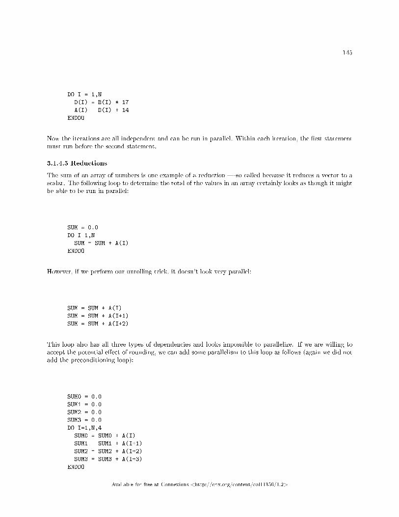
145
DO I = 1,N
D(I) = B(I) * 17
A(I) = D(I) + 14
ENDDO
Now the iterations are all independent and can be run in parallel. Within each iteration, the �rst statementmust run before the second statement.
3.1.4.5 Reductions
The sum of an array of numbers is one example of a reduction � so called because it reduces a vector to ascalar. The following loop to determine the total of the values in an array certainly looks as though it mightbe able to be run in parallel:
SUM = 0.0
DO I=1,N
SUM = SUM + A(I)
ENDDO
However, if we perform our unrolling trick, it doesn't look very parallel:
SUM = SUM + A(I)
SUM = SUM + A(I+1)
SUM = SUM + A(I+2)
This loop also has all three types of dependencies and looks impossible to parallelize. If we are willing toaccept the potential e�ect of rounding, we can add some parallelism to this loop as follows (again we did notadd the preconditioning loop):
SUM0 = 0.0
SUM1 = 0.0
SUM2 = 0.0
SUM3 = 0.0
DO I=1,N,4
SUM0 = SUM0 + A(I)
SUM1 = SUM1 + A(I+1)
SUM2 = SUM2 + A(I+2)
SUM3 = SUM3 + A(I+3)
ENDDO
Available for free at Connexions <http://cnx.org/content/col11356/1.2>
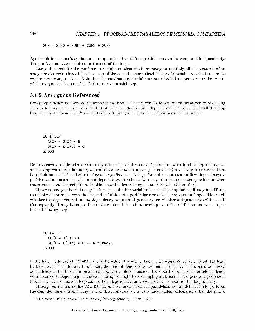
146 CHAPTER 3. PROCESADORES PARALELOS DE MEMORIA COMPARTIDA
SUM = SUM0 + SUM1 + SUM2 + SUM3
Again, this is not precisely the same computation, but all four partial sums can be computed independently.The partial sums are combined at the end of the loop.
Loops that look for the maximum or minimum elements in an array, or multiply all the elements of anarray, are also reductions. Likewise, some of these can be reorganized into partial results, as with the sum, toexpose more computations. Note that the maximum and minimum are associative operators, so the resultsof the reorganized loop are identical to the sequential loop.
3.1.5 Ambiguous References8
Every dependency we have looked at so far has been clear cut; you could see exactly what you were dealingwith by looking at the source code. But other times, describing a dependency isn't so easy. Recall this loopfrom the �Antidependencies� section Section 3.1.4.2 (Antidependencies) earlier in this chapter:
DO I=1,N
A(I) = B(I) * E
B(I) = A(I+2) * C
ENDDO
Because each variable reference is solely a function of the index, I, it's clear what kind of dependency weare dealing with. Furthermore, we can describe how far apart (in iterations) a variable reference is fromits de�nition. This is called the dependency distance. A negative value represents a �ow dependency; apositive value means there is an antidependency. A value of zero says that no dependency exists betweenthe reference and the de�nition. In this loop, the dependency distance for A is +2 iterations.
However, array subscripts may be functions of other variables besides the loop index. It may be di�cultto tell the distance between the use and de�nition of a particular element. It may even be impossible to tellwhether the dependency is a �ow dependency or an antidependency, or whether a dependency exists at all.Consequently, it may be impossible to determine if it's safe to overlap execution of di�erent statements, asin the following loop:
DO I=1,N
A(I) = B(I) * E
B(I) = A(I+K) * C ← K unknown
ENDDO
If the loop made use of A(I+K), where the value of K was unknown, we wouldn't be able to tell (at leastby looking at the code) anything about the kind of dependency we might be facing. If K is zero, we have adependency within the iteration and no loop-carried dependencies. If K is positive we have an antidependencywith distance K. Depending on the value for K, we might have enough parallelism for a superscalar processor.If K is negative, we have a loop-carried �ow dependency, and we may have to execute the loop serially.
Ambiguous references, like A(I+K) above, have an e�ect on the parallelism we can detect in a loop. Fromthe compiler perspective, it may be that this loop does contain two independent calculations that the author
8This content is available online at <http://cnx.org/content/m32788/1.3/>.
Available for free at Connexions <http://cnx.org/content/col11356/1.2>
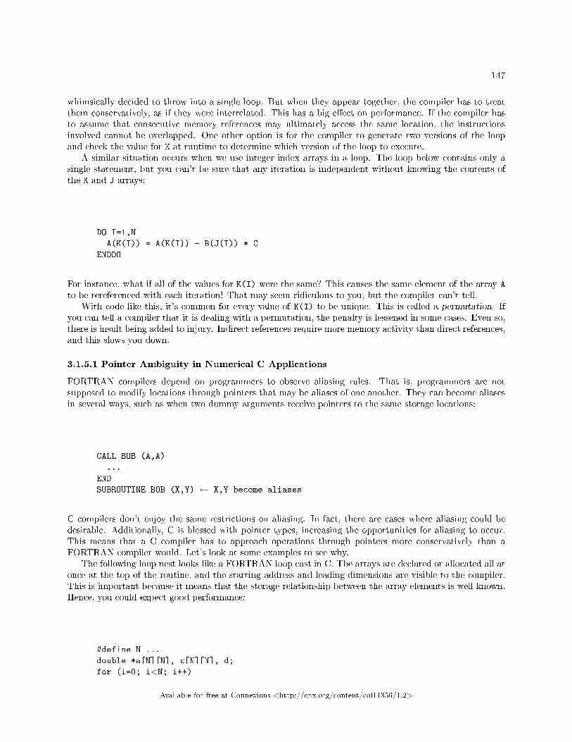
147
whimsically decided to throw into a single loop. But when they appear together, the compiler has to treatthem conservatively, as if they were interrelated. This has a big e�ect on performance. If the compiler hasto assume that consecutive memory references may ultimately access the same location, the instructionsinvolved cannot be overlapped. One other option is for the compiler to generate two versions of the loopand check the value for K at runtime to determine which version of the loop to execute.
A similar situation occurs when we use integer index arrays in a loop. The loop below contains only asingle statement, but you can't be sure that any iteration is independent without knowing the contents ofthe K and J arrays:
DO I=1,N
A(K(I)) = A(K(I)) + B(J(I)) * C
ENDDO
For instance, what if all of the values for K(I) were the same? This causes the same element of the array A
to be rereferenced with each iteration! That may seem ridiculous to you, but the compiler can't tell.With code like this, it's common for every value of K(I) to be unique. This is called a permutation. If
you can tell a compiler that it is dealing with a permutation, the penalty is lessened in some cases. Even so,there is insult being added to injury. Indirect references require more memory activity than direct references,and this slows you down.
3.1.5.1 Pointer Ambiguity in Numerical C Applications
FORTRAN compilers depend on programmers to observe aliasing rules. That is, programmers are notsupposed to modify locations through pointers that may be aliases of one another. They can become aliasesin several ways, such as when two dummy arguments receive pointers to the same storage locations:
CALL BOB (A,A)
...
END
SUBROUTINE BOB (X,Y) ← X,Y become aliases
C compilers don't enjoy the same restrictions on aliasing. In fact, there are cases where aliasing could bedesirable. Additionally, C is blessed with pointer types, increasing the opportunities for aliasing to occur.This means that a C compiler has to approach operations through pointers more conservatively than aFORTRAN compiler would. Let's look at some examples to see why.
The following loop nest looks like a FORTRAN loop cast in C. The arrays are declared or allocated all atonce at the top of the routine, and the starting address and leading dimensions are visible to the compiler.This is important because it means that the storage relationship between the array elements is well known.Hence, you could expect good performance:
#define N ...
double *a[N][N], c[N][N], d;
for (i=0; i<N; i++)
Available for free at Connexions <http://cnx.org/content/col11356/1.2>
148 CHAPTER 3. PROCESADORES PARALELOS DE MEMORIA COMPARTIDA
for (j=0; j<N; j++)
a[i][j] = a[i][j] + c[j][i] * d;
Now imagine what happens if you allocate the rows dynamically. This makes the address calculations morecomplicated. The loop nest hasn't changed; however, there is no guaranteed stride that can get you fromone row to the next. This is because the storage relationship between the rows is unknown:
#define N ...
double *a[N], *c[N], d;
for (i=0; i<N; i++) {
a[i] = (double *) malloc (N*sizeof(double));
c[i] = (double *) malloc (N*sizeof(double));
}
for (i=0; i<N; i++)
for (j=0; j<N; j++)
a[i][j] = a[i][j] + c[j][i] * d;
In fact, your compiler knows even less than you might expect about the storage relationship. For instance,how can it be sure that references to a and c aren't aliases? It may be obvious to you that they're not. Youmight point out that malloc never overlaps storage. But the compiler isn't free to assume that. Who knows?You may be substituting your own version of malloc!
Let's look at a di�erent example, where storage is allocated all at once, though the declarations are notvisible to all routines that are using it. The following subroutine bob performs the same computation asour previous example. However, because the compiler can't see the declarations for a and c (they're in themain routine), it doesn't have enough information to be able to overlap memory references from successiveiterations; the references could be aliases:
#define N...
main()
{
double a[N][N], c[N][N], d;
...
bob (a,c,d,N);
}
bob (double *a,double *c,double d,int n)
{
int i,j;
double *ap, *cp;
for (i=0;i<n;i++) {
ap = a + (i*n);
cp = c + i;
for (j=0; j<n; j++)
*(ap+j) = *(ap+j) + *(cp+(j*n)) * d;
}
}
Available for free at Connexions <http://cnx.org/content/col11356/1.2>
149
To get the best performance, make available to the compiler as many details about the size and shape of yourdata structures as possible. Pointers, whether in the form of formal arguments to a subroutine or explicitlydeclared, can hide important facts about how you are using memory. The more information the compilerhas, the more it can overlap memory references. This information can come from compiler directives or frommaking declarations visible in the routines where performance is most critical.
3.1.6 Closing Notes9
You already knew there was a limit to the amount of parallelism in any given program. Now you knowwhy. Clearly, if a program had no dependencies, you could execute the whole thing at once, given suitablehardware. But programs aren't in�nitely parallel; they are often hardly parallel at all. This is because theycontain dependencies of the types we saw above.
When we are writing and/or tuning our loops, we have a number of (sometimes con�icting) goals to keepin mind:
• Balance memory operations and computations.• Minimize unnecessary operations.• Access memory using unit stride if at all possible.• Allow all of the loop iterations to be computed in parallel.
In the coming chapters, we will begin to learn more about executing our programs on parallel multiprocessors.At some point we will escape the bonds of compiler automatic optimization and begin to explicitly code theparallel portions of our code.
To learn more about compilers and data�ow, read The Art of Compiler Design: Theory and Practice byThomas Pittman and James Peters (Prentice-Hall).
3.1.7 Exercises10
Exercise 3.1.7.1Identify the dependencies (if there are any) in the following loops. Can you think of ways toorganize each loop for more parallelism?
a.
DO I=1,N-2
A(I+2) = A(I) + 1.
ENDDO
b.
DO I=1,N-1,2
A(I+1) = A(I) + 1.
ENDDO
c.9This content is available online at <http://cnx.org/content/m32789/1.3/>.
10This content is available online at <http://cnx.org/content/m32792/1.3/>.
Available for free at Connexions <http://cnx.org/content/col11356/1.2>
150 CHAPTER 3. PROCESADORES PARALELOS DE MEMORIA COMPARTIDA
DO I=2,N
A(I) = A(I-1) * 2.
B = A(I-1)
ENDDO
d.
DO I=1,N
IF(N .GT. M)
A(I) = 1.
ENDDO
e.
DO I=1,N
A(I,J) = A(I,K) + B
ENDDO
f.
DO I=1,N-1
A(I+1,J) = A(I,K) + B
ENDDO
g.
for (i=0; i<n; i++)
a[i] = b[i];
Exercise 3.1.7.2Imagine that you are a parallelizing compiler, trying to generate code for the loop below. Why arereferences to A a challenge? Why would it help to know that K is equal to zero? Explain how youcould partially vectorize the statements involving A if you knew that K had an absolute value ofat least 8.
DO I=1,N
Available for free at Connexions <http://cnx.org/content/col11356/1.2>
151
E(I,M) = E(I-1,M+1) - 1.0
B(I) = A(I+K) * C
A(I) = D(I) * 2.0
ENDDO
Exercise 3.1.7.3The following three statements contain a �ow dependency, an antidependency and an outputdependency. Can you identify each? Given that you are allowed to reorder the statements, can you�nd a permutation that produces the same values for the variables C and B? Show how you canreduce the dependencies by combining or rearranging calculations and using temporary variables.
B = A + C
B = C + D
C = B + D
3.2 Shared-Memory Multiprocessors
3.2.1 Introduction11
In the mid-1980s, shared-memory multiprocessors were pretty expensive and pretty rare. Now, as hardwarecosts are dropping, they are becoming commonplace. Many home computer systems in the under-$3000range have a socket for a second CPU. Home computer operating systems are providing the capability to usemore than one processor to improve system performance. Rather than specialized resources locked away ina central computing facility, these shared-memory processors are often viewed as a logical extension of thedesktop. These systems run the same operating system (UNIX or NT) as the desktop and many of the sameapplications from a workstation will execute on these multiprocessor servers.
Typically a workstation will have from 1 to 4 processors and a server system will have 4 to 64 processors.Shared-memory multiprocessors have a signi�cant advantage over other multiprocessors because all theprocessors share the same view of the memory, as shown in Figure 3.11 (A shared-memory multiprocessor).
These processors are also described as uniform memory access (also known as UMA) systems. Thisdesignation indicates that memory is equally accessible to all processors with the same performance.
The popularity of these systems is not due simply to the demand for high performance computing. Thesesystems are excellent at providing high throughput for a multiprocessing load, and function e�ectively ashigh-performance database servers, network servers, and Internet servers. Within limits, their throughputis increased linearly as more processors are added.
In this book we are not so interested in the performance of database or Internet servers. That is toopassé; buy more processors, get better throughput. We are interested in pure, raw, unadulterated computespeed for our high performance application. Instead of running hundreds of small jobs, we want to utilizeall $750,000 worth of hardware for our single job.
The challenge is to �nd techniques that make a program that takes an hour to complete using oneprocessor, complete in less than a minute using 64 processors. This is not trivial. Throughout this book sofar, we have been on an endless quest for parallelism. In this and the remaining chapters, we will begin tosee the payo� for all of your hard work and dedication!
11This content is available online at <http://cnx.org/content/m32797/1.3/>.
Available for free at Connexions <http://cnx.org/content/col11356/1.2>
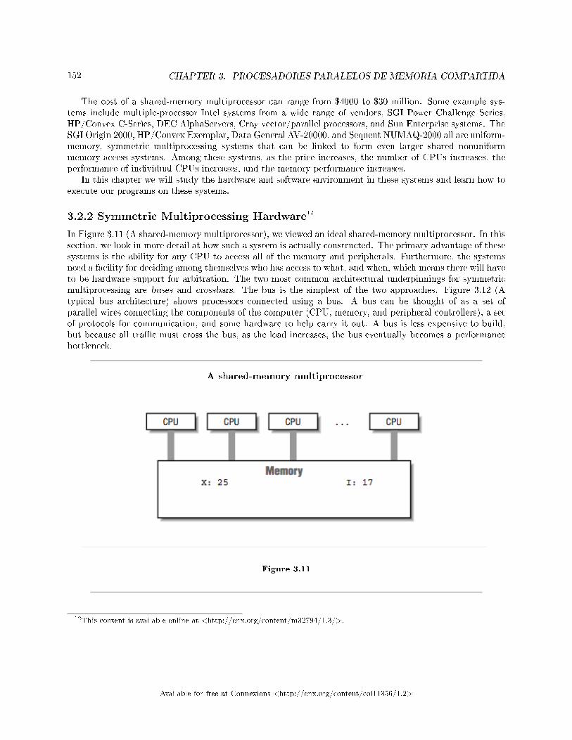
152 CHAPTER 3. PROCESADORES PARALELOS DE MEMORIA COMPARTIDA
The cost of a shared-memory multiprocessor can range from $4000 to $30 million. Some example sys-tems include multiple-processor Intel systems from a wide range of vendors, SGI Power Challenge Series,HP/Convex C-Series, DEC AlphaServers, Cray vector/parallel processors, and Sun Enterprise systems. TheSGI Origin 2000, HP/Convex Exemplar, Data General AV-20000, and Sequent NUMAQ-2000 all are uniform-memory, symmetric multiprocessing systems that can be linked to form even larger shared nonuniformmemory-access systems. Among these systems, as the price increases, the number of CPUs increases, theperformance of individual CPUs increases, and the memory performance increases.
In this chapter we will study the hardware and software environment in these systems and learn how toexecute our programs on these systems.
3.2.2 Symmetric Multiprocessing Hardware12
In Figure 3.11 (A shared-memory multiprocessor), we viewed an ideal shared-memory multiprocessor. In thissection, we look in more detail at how such a system is actually constructed. The primary advantage of thesesystems is the ability for any CPU to access all of the memory and peripherals. Furthermore, the systemsneed a facility for deciding among themselves who has access to what, and when, which means there will haveto be hardware support for arbitration. The two most common architectural underpinnings for symmetricmultiprocessing are buses and crossbars. The bus is the simplest of the two approaches. Figure 3.12 (Atypical bus architecture) shows processors connected using a bus. A bus can be thought of as a set ofparallel wires connecting the components of the computer (CPU, memory, and peripheral controllers), a setof protocols for communication, and some hardware to help carry it out. A bus is less expensive to build,but because all tra�c must cross the bus, as the load increases, the bus eventually becomes a performancebottleneck.
A shared-memory multiprocessor
Figure 3.11
12This content is available online at <http://cnx.org/content/m32794/1.3/>.
Available for free at Connexions <http://cnx.org/content/col11356/1.2>
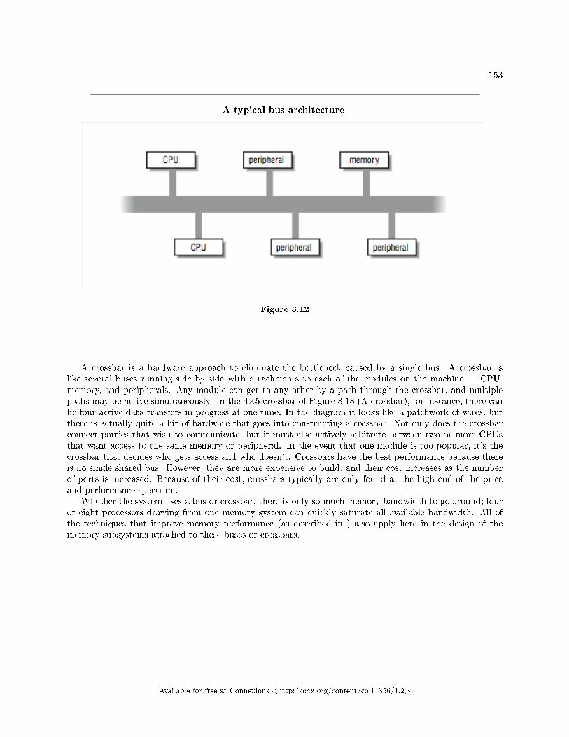
153
A typical bus architecture
Figure 3.12
A crossbar is a hardware approach to eliminate the bottleneck caused by a single bus. A crossbar islike several buses running side by side with attachments to each of the modules on the machine � CPU,memory, and peripherals. Any module can get to any other by a path through the crossbar, and multiplepaths may be active simultaneously. In the 4×5 crossbar of Figure 3.13 (A crossbar), for instance, there canbe four active data transfers in progress at one time. In the diagram it looks like a patchwork of wires, butthere is actually quite a bit of hardware that goes into constructing a crossbar. Not only does the crossbarconnect parties that wish to communicate, but it must also actively arbitrate between two or more CPUsthat want access to the same memory or peripheral. In the event that one module is too popular, it's thecrossbar that decides who gets access and who doesn't. Crossbars have the best performance because thereis no single shared bus. However, they are more expensive to build, and their cost increases as the numberof ports is increased. Because of their cost, crossbars typically are only found at the high end of the priceand performance spectrum.
Whether the system uses a bus or crossbar, there is only so much memory bandwidth to go around; fouror eight processors drawing from one memory system can quickly saturate all available bandwidth. All ofthe techniques that improve memory performance (as described in ) also apply here in the design of thememory subsystems attached to these buses or crossbars.
Available for free at Connexions <http://cnx.org/content/col11356/1.2>
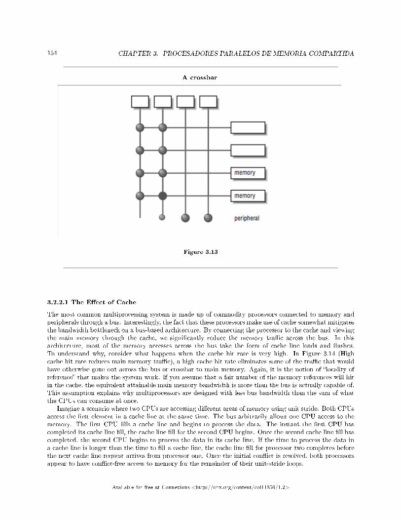
154 CHAPTER 3. PROCESADORES PARALELOS DE MEMORIA COMPARTIDA
A crossbar
Figure 3.13
3.2.2.1 The E�ect of Cache
The most common multiprocessing system is made up of commodity processors connected to memory andperipherals through a bus. Interestingly, the fact that these processors make use of cache somewhat mitigatesthe bandwidth bottleneck on a bus-based architecture. By connecting the processor to the cache and viewingthe main memory through the cache, we signi�cantly reduce the memory tra�c across the bus. In thisarchitecture, most of the memory accesses across the bus take the form of cache line loads and �ushes.To understand why, consider what happens when the cache hit rate is very high. In Figure 3.14 (Highcache hit rate reduces main memory tra�c), a high cache hit rate eliminates some of the tra�c that wouldhave otherwise gone out across the bus or crossbar to main memory. Again, it is the notion of �locality ofreference� that makes the system work. If you assume that a fair number of the memory references will hitin the cache, the equivalent attainable main memory bandwidth is more than the bus is actually capable of.This assumption explains why multiprocessors are designed with less bus bandwidth than the sum of whatthe CPUs can consume at once.
Imagine a scenario where two CPUs are accessing di�erent areas of memory using unit stride. Both CPUsaccess the �rst element in a cache line at the same time. The bus arbitrarily allows one CPU access to thememory. The �rst CPU �lls a cache line and begins to process the data. The instant the �rst CPU hascompleted its cache line �ll, the cache line �ll for the second CPU begins. Once the second cache line �ll hascompleted, the second CPU begins to process the data in its cache line. If the time to process the data ina cache line is longer than the time to �ll a cache line, the cache line �ll for processor two completes beforethe next cache line request arrives from processor one. Once the initial con�ict is resolved, both processorsappear to have con�ict-free access to memory for the remainder of their unit-stride loops.
Available for free at Connexions <http://cnx.org/content/col11356/1.2>
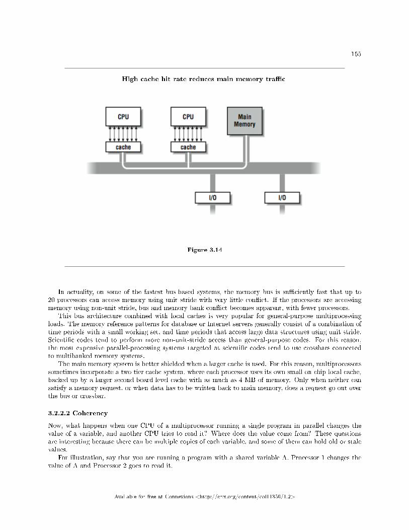
155
High cache hit rate reduces main memory tra�c
Figure 3.14
In actuality, on some of the fastest bus-based systems, the memory bus is su�ciently fast that up to20 processors can access memory using unit stride with very little con�ict. If the processors are accessingmemory using non-unit stride, bus and memory bank con�ict becomes apparent, with fewer processors.
This bus architecture combined with local caches is very popular for general-purpose multiprocessingloads. The memory reference patterns for database or Internet servers generally consist of a combination oftime periods with a small working set, and time periods that access large data structures using unit stride.Scienti�c codes tend to perform more non-unit-stride access than general-purpose codes. For this reason,the most expensive parallel-processing systems targeted at scienti�c codes tend to use crossbars connectedto multibanked memory systems.
The main memory system is better shielded when a larger cache is used. For this reason, multiprocessorssometimes incorporate a two-tier cache system, where each processor uses its own small on-chip local cache,backed up by a larger second board-level cache with as much as 4 MB of memory. Only when neither cansatisfy a memory request, or when data has to be written back to main memory, does a request go out overthe bus or crossbar.
3.2.2.2 Coherency
Now, what happens when one CPU of a multiprocessor running a single program in parallel changes thevalue of a variable, and another CPU tries to read it? Where does the value come from? These questionsare interesting because there can be multiple copies of each variable, and some of them can hold old or stalevalues.
For illustration, say that you are running a program with a shared variable A. Processor 1 changes thevalue of A and Processor 2 goes to read it.
Available for free at Connexions <http://cnx.org/content/col11356/1.2>
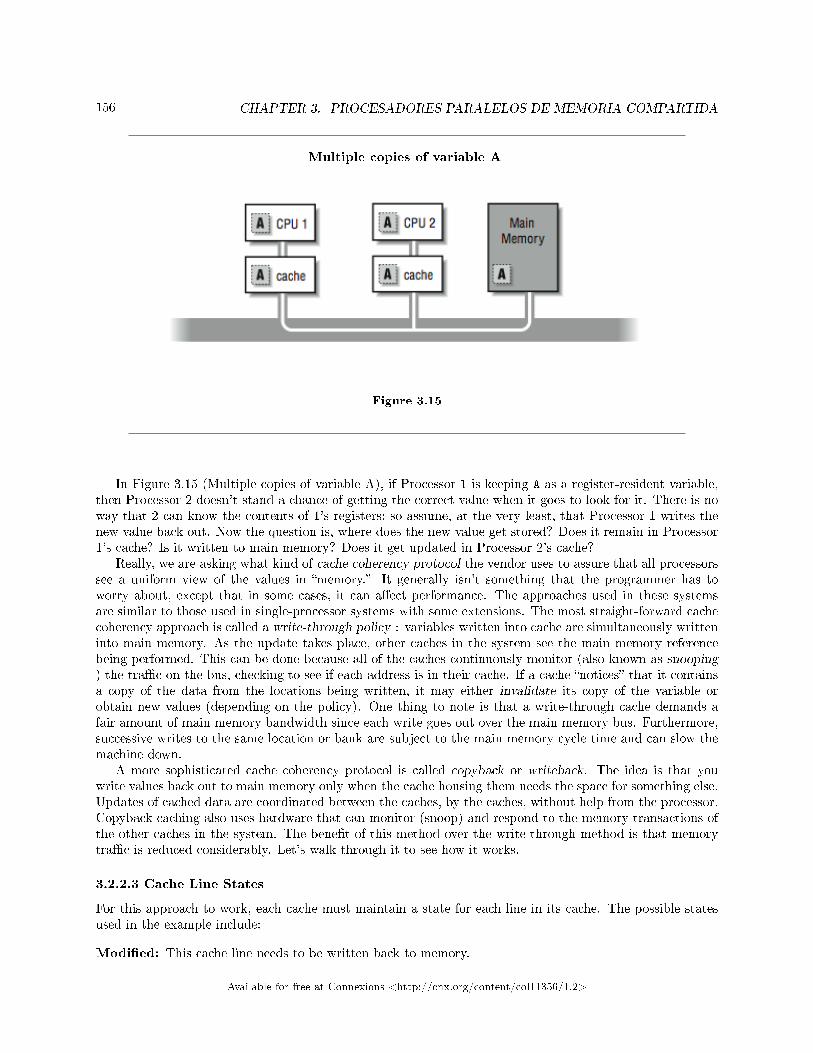
156 CHAPTER 3. PROCESADORES PARALELOS DE MEMORIA COMPARTIDA
Multiple copies of variable A
Figure 3.15
In Figure 3.15 (Multiple copies of variable A), if Processor 1 is keeping A as a register-resident variable,then Processor 2 doesn't stand a chance of getting the correct value when it goes to look for it. There is noway that 2 can know the contents of 1's registers; so assume, at the very least, that Processor 1 writes thenew value back out. Now the question is, where does the new value get stored? Does it remain in Processor1's cache? Is it written to main memory? Does it get updated in Processor 2's cache?
Really, we are asking what kind of cache coherency protocol the vendor uses to assure that all processorssee a uniform view of the values in �memory.� It generally isn't something that the programmer has toworry about, except that in some cases, it can a�ect performance. The approaches used in these systemsare similar to those used in single-processor systems with some extensions. The most straight-forward cachecoherency approach is called a write-through policy : variables written into cache are simultaneously writteninto main memory. As the update takes place, other caches in the system see the main memory referencebeing performed. This can be done because all of the caches continuously monitor (also known as snooping) the tra�c on the bus, checking to see if each address is in their cache. If a cache �notices� that it containsa copy of the data from the locations being written, it may either invalidate its copy of the variable orobtain new values (depending on the policy). One thing to note is that a write-through cache demands afair amount of main memory bandwidth since each write goes out over the main memory bus. Furthermore,successive writes to the same location or bank are subject to the main memory cycle time and can slow themachine down.
A more sophisticated cache coherency protocol is called copyback or writeback. The idea is that youwrite values back out to main memory only when the cache housing them needs the space for something else.Updates of cached data are coordinated between the caches, by the caches, without help from the processor.Copyback caching also uses hardware that can monitor (snoop) and respond to the memory transactions ofthe other caches in the system. The bene�t of this method over the write-through method is that memorytra�c is reduced considerably. Let's walk through it to see how it works.
3.2.2.3 Cache Line States
For this approach to work, each cache must maintain a state for each line in its cache. The possible statesused in the example include:
Modi�ed: This cache line needs to be written back to memory.
Available for free at Connexions <http://cnx.org/content/col11356/1.2>
157
Exclusive: There are no other caches that have this cache line.Shared: There are read-only copies of this line in two or more caches.Empty/Invalid: This cache line doesn't contain any useful data.
This particular coherency protocol is often called MESI. Other cache coherency protocols are more compli-cated, but these states give you an idea how multiprocessor writeback cache coherency works.
We start where a particular cache line is in memory and in none of the writeback caches on the systems.The �rst cache to ask for data from a particular part of memory completes a normal memory access; themain memory system returns data from the requested location in response to a cache miss. The associatedcache line is marked exclusive, meaning that this is the only cache in the system containing a copy of thedata; it is the owner of the data. If another cache goes to main memory looking for the same thing, therequest is intercepted by the �rst cache, and the data is returned from the �rst cache � not main memory.Once an interception has occurred and the data is returned, the data is marked shared in both of the caches.
When a particular line is marked shared, the caches have to treat it di�erently than they would if theywere the exclusive owners of the data � especially if any of them wants to modify it. In particular, a write toa shared cache entry is preceded by a broadcast message to all the other caches in the system. It tells themto invalidate their copies of the data. The one remaining cache line gets marked as modi�ed to signal thatit has been changed, and that it must be returned to main memory when the space is needed for somethingelse. By these mechanisms, you can maintain cache coherence across the multiprocessor without addingtremendously to the memory tra�c.
By the way, even if a variable is not shared, it's possible for copies of it to show up in several caches.On a symmetric multiprocessor, your program can bounce around from CPU to CPU. If you run for a littlewhile on this CPU, and then a little while on that, your program will have operated out of separate caches.That means that there can be several copies of seemingly unshared variables scattered around the machine.Operating systems often try to minimize how often a process is moved between physical CPUs during contextswitches. This is one reason not to overload the available processors in a system.
3.2.2.4 Data Placement
There is one more pitfall regarding shared memory we have so far failed to mention. It involves datamovement. Although it would be convenient to think of the multiprocessor memory as one big pool, we haveseen that it is actually a carefully crafted system of caches, coherency protocols, and main memory. Theproblems come when your application causes lots of data to be traded between the caches. Each referencethat falls out of a given processor's cache (especially those that require an update in another processor'scache) has to go out on the bus.
Often, it's slower to get memory from another processor's cache than from the main memory because ofthe protocol and processing overhead involved. Not only do we need to have programs with high locality ofreference and unit stride, we also need to minimize the data that must be moved from one CPU to another.
3.2.3 Multiprocessor Software Concepts 13
Now that we have examined the way shared-memory multiprocessor hardware operates, we need to examinehow software operates on these types of computers. We still have to wait until the next chapters to beginmaking our FORTRAN programs run in parallel. For now, we use C programs to examine the fundamentalsof multiprocessing and multithreading. There are several techniques used to implement multithreading, sothe topics we will cover include:
• Operating system�supported multiprocessing• User space multithreading• Operating system-supported multithreading
The last of these is what we primarily will use to reduce the walltime of our applications.13This content is available online at <http://cnx.org/content/m32800/1.3/>.
Available for free at Connexions <http://cnx.org/content/col11356/1.2>
158 CHAPTER 3. PROCESADORES PARALELOS DE MEMORIA COMPARTIDA
3.2.3.1 Operating System�Supported Multiprocessing
Most modern general-purpose operating systems support some form of multiprocessing. Multiprocessingdoesn't require more than one physical CPU; it is simply the operating system's ability to run more thanone process on the system. The operating system context-switches between each process at �xed timeintervals, or on interrupts or input-output activity. For example, in UNIX, if you use the ps command, youcan see the processes on the system:
% ps -a
PID TTY TIME CMD
28410 pts/34 0:00 tcsh
28213 pts/38 0:00 xterm
10488 pts/51 0:01 telnet
28411 pts/34 0:00 xbiff
11123 pts/25 0:00 pine
3805 pts/21 0:00 elm
6773 pts/44 5:48 ansys
...
% ps --a | grep ansys
6773 pts/44 6:00 ansys
For each process we see the process identi�er (PID), the terminal that is executing the command, the amountof CPU time the command has used, and the name of the command. The PID is unique across the entiresystem. Most UNIX commands are executed in a separate process. In the above example, most of theprocesses are waiting for some type of event, so they are taking very few resources except for memory.Process 677314 seems to be executing and using resources. Running ps again con�rms that the CPU time isincreasing for the ansys process:
% vmstat 5
procs memory page disk faults cpu
r b w swap free re mf pi po fr de sr f0 s0 -- -- in sy cs us sy id
3 0 0 353624 45432 0 0 1 0 0 0 0 0 0 0 0 461 5626 354 91 9 0
3 0 0 353248 43960 0 22 0 0 0 0 0 0 14 0 0 518 6227 385 89 11 0
Running the vmstat 5 command tells us many things about the activity on the system. First, there arethree runnable processes. If we had one CPU, only one would actually be running at a given instant. Toallow all three jobs to progress, the operating system time-shares between the processes. Assuming equalpriority, each process executes about 1/3 of the time. However, this system is a two-processor system, soeach process executes about 2/3 of the time. Looking across the vmstat output, we can see paging activity(pi, po), context switches (cs), overall user time (us), system time (sy), and idle time (id ).
Each process can execute a completely di�erent program. While most processes are completely inde-pendent, they can cooperate and share information using interprocess communication (pipes, sockets) orvarious operating system-supported shared-memory areas. We generally don't use multiprocessing on theseshared-memory systems as a technique to increase single-application performance.
14ANSYS is a commonly used structural-analysis package.
Available for free at Connexions <http://cnx.org/content/col11356/1.2>
159
3.2.3.2 Multiprocessing software
In this section, we explore how programs access multiprocessing features.15 In this example, the programcreates a new process using the fork( ) function. The new process (child) prints some messages and thenchanges its identity using exec( ) by loading a new program. The original process (parent) prints somemessages and then waits for the child process to complete:
int globvar; /* A global variable */
main () {
int pid,status,retval;
int stackvar; /* A stack variable */
globvar = 1;
stackvar = 1;
printf("Main - calling fork globvar=%d stackvar=%d\n",globvar,stackvar);pid = fork();
printf("Main - fork returned pid=%d\n",pid);if ( pid == 0 ) {
printf("Child - globvar=%d stackvar=%d\n",globvar,stackvar);sleep(1);
printf("Child - woke up globvar=%d stackvar=%d\n",globvar,stackvar);globvar = 100;
stackvar = 100;
printf("Child - modified globvar=%d stackvar=%d\n",globvar,stackvar);retval = execl("/bin/date", (char *) 0 );
printf("Child - WHY ARE WE HERE retval=%d\n",retval);} else {
printf("Parent - globvar=%d stackvar=%d\n",globvar,stackvar);globvar = 5;
stackvar = 5;
printf("Parent - sleeping globvar=%d stackvar=%d\n",globvar,stackvar);sleep(2);
printf("Parent - woke up globvar=%d stackvar=%d\n",globvar,stackvar);printf("Parent - waiting for pid=%d\n",pid);retval = wait(&status);
status = status � 8; /* Return code in bits 15-8 */
printf("Parent - status=%d retval=%d\n",status,retval);}
}
The key to understanding this code is to understand how the fork( ) function operates. The simplesummary is that the fork( ) function is called once in a process and returns twice, once in the originalprocess and once in a newly created process. The newly created process is an identical copy of the originalprocess. All the variables (local and global) have been duplicated. Both processes have access to all of theopen �les of the original process. Figure 3.16 (How a fork operates) shows how the fork operation creates anew process.
15These examples are written in C using the POSIX 1003.1 application programming interface. This example runs on mostUNIX systems and on other POSIX-compliant systems including OpenNT, Open- VMS, and many others.
Available for free at Connexions <http://cnx.org/content/col11356/1.2>
160 CHAPTER 3. PROCESADORES PARALELOS DE MEMORIA COMPARTIDA
The only di�erence between the processes is that the return value from the fork( ) function call is 0in the new (child) process and the process identi�er (shown by the ps command) in the original (parent)process. This is the program output:
recs % cc -o fork fork.c
recs % fork
Main - calling fork globvar=1 stackvar=1
Main - fork returned pid=19336
Main - fork returned pid=0
Parent - globvar=1 stackvar=1
Parent - sleeping globvar=5 stackvar=5
Child - globvar=1 stackvar=1
Child - woke up globvar=1 stackvar=1
Child - modified globvar=100 stackvar=100
Thu Nov 6 22:40:33
Parent - woke up globvar=5 stackvar=5
Parent - waiting for pid=19336
Parent - status=0 retval=19336
recs %
Tracing this through, �rst the program sets the global and stack variable to one and then calls fork( ).During the fork( ) call, the operating system suspends the process, makes an exact duplicate of the process,and then restarts both processes. You can see two messages from the statement immediately after the fork.The �rst line is coming from the original process, and the second line is coming from the new process. If youwere to execute a ps command at this moment in time, you would see two processes running called �fork.�One would have a process identi�er of 19336.
Available for free at Connexions <http://cnx.org/content/col11356/1.2>
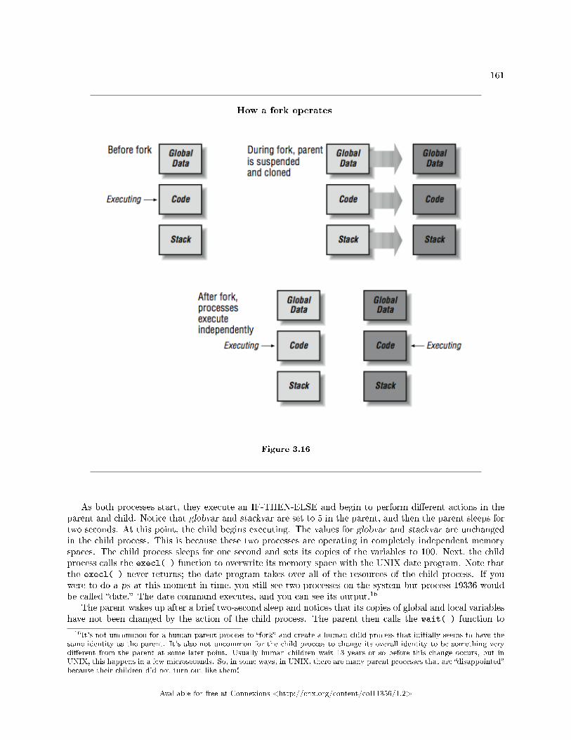
161
How a fork operates
Figure 3.16
As both processes start, they execute an IF-THEN-ELSE and begin to perform di�erent actions in theparent and child. Notice that globvar and stackvar are set to 5 in the parent, and then the parent sleeps fortwo seconds. At this point, the child begins executing. The values for globvar and stackvar are unchangedin the child process. This is because these two processes are operating in completely independent memoryspaces. The child process sleeps for one second and sets its copies of the variables to 100. Next, the childprocess calls the execl( ) function to overwrite its memory space with the UNIX date program. Note thatthe execl( ) never returns; the date program takes over all of the resources of the child process. If youwere to do a ps at this moment in time, you still see two processes on the system but process 19336 wouldbe called �date.� The date command executes, and you can see its output.16
The parent wakes up after a brief two-second sleep and notices that its copies of global and local variableshave not been changed by the action of the child process. The parent then calls the wait( ) function to
16It's not uncommon for a human parent process to �fork� and create a human child process that initially seems to have thesame identity as the parent. It's also not uncommon for the child process to change its overall identity to be something verydi�erent from the parent at some later point. Usually human children wait 13 years or so before this change occurs, but inUNIX, this happens in a few microseconds. So, in some ways, in UNIX, there are many parent processes that are �disappointed�because their children did not turn out like them!
Available for free at Connexions <http://cnx.org/content/col11356/1.2>
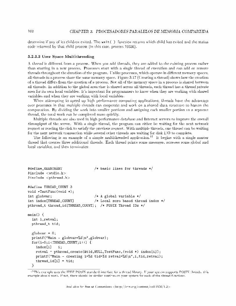
162 CHAPTER 3. PROCESADORES PARALELOS DE MEMORIA COMPARTIDA
determine if any of its children exited. The wait( ) function returns which child has exited and the statuscode returned by that child process (in this case, process 19336).
3.2.3.3 User Space Multithreading
A thread is di�erent from a process. When you add threads, they are added to the existing process ratherthan starting in a new process. Processes start with a single thread of execution and can add or removethreads throughout the duration of the program. Unlike processes, which operate in di�erent memory spaces,all threads in a process share the same memory space. Figure 3.17 (Creating a thread) shows how the creationof a thread di�ers from the creation of a process. Not all of the memory space in a process is shared betweenall threads. In addition to the global area that is shared across all threads, each thread has a thread privatearea for its own local variables. It's important for programmers to know when they are working with sharedvariables and when they are working with local variables.
When attempting to speed up high performance computing applications, threads have the advantageover processes in that multiple threads can cooperate and work on a shared data structure to hasten thecomputation. By dividing the work into smaller portions and assigning each smaller portion to a separatethread, the total work can be completed more quickly.
Multiple threads are also used in high performance database and Internet servers to improve the overallthroughput of the server. With a single thread, the program can either be waiting for the next networkrequest or reading the disk to satisfy the previous request. With multiple threads, one thread can be waitingfor the next network transaction while several other threads are waiting for disk I/O to complete.
The following is an example of a simple multithreaded application.17 It begins with a single masterthread that creates three additional threads. Each thread prints some messages, accesses some global andlocal variables, and then terminates:
#define_REENTRANT /* basic lines for threads */
#include <stdio.h>#include <pthread.h>
#define THREAD_COUNT 3
void *TestFunc(void *);
int globvar; /* A global variable */
int index[THREAD_COUNT] /* Local zero-based thread index */
pthread_t thread_id[THREAD_COUNT]; /* POSIX Thread IDs */
main() {
int i,retval;
pthread_t tid;
globvar = 0;
printf("Main - globvar=%d\n",globvar);for(i=0;i<THREAD_COUNT;i++) {
index[i] = i;
retval = pthread_create(&tid,NULL,TestFunc,(void *) index[i]);
printf("Main - creating i=%d tid=%d retval=%d\n",i,tid,retval);thread_id[i] = tid;
}
17This example uses the IEEE POSIX standard interface for a thread library. If your system supports POSIX threads, thisexample should work. If not, there should be similar routines on your system for each of the thread functions.
Available for free at Connexions <http://cnx.org/content/col11356/1.2>
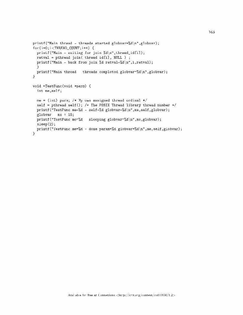
163
printf("Main thread - threads started globvar=%d\n",globvar);for(i=0;i<THREAD_COUNT;i++) {
printf("Main - waiting for join %d\n",thread_id[i]);retval = pthread_join( thread_id[i], NULL ) ;
printf("Main - back from join %d retval=%d\n",i,retval);}
printf("Main thread - threads completed globvar=%d\n",globvar);}
void *TestFunc(void *parm) {
int me,self;
me = (int) parm; /* My own assigned thread ordinal */
self = pthread_self(); /* The POSIX Thread library thread number */
printf("TestFunc me=%d - self=%d globvar=%d\n",me,self,globvar);globvar = me + 15;
printf("TestFunc me=%d - sleeping globvar=%d\n",me,globvar);sleep(2);
printf("TestFunc me=%d - done param=%d globvar=%d\n",me,self,globvar);}
Available for free at Connexions <http://cnx.org/content/col11356/1.2>
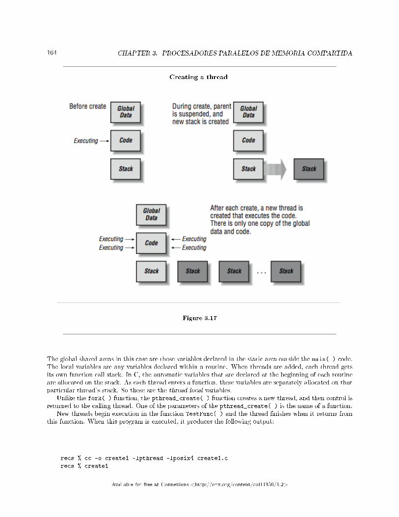
164 CHAPTER 3. PROCESADORES PARALELOS DE MEMORIA COMPARTIDA
Creating a thread
Figure 3.17
The global shared areas in this case are those variables declared in the static area outside the main( ) code.The local variables are any variables declared within a routine. When threads are added, each thread getsits own function call stack. In C, the automatic variables that are declared at the beginning of each routineare allocated on the stack. As each thread enters a function, these variables are separately allocated on thatparticular thread's stack. So these are the thread-local variables.
Unlike the fork( ) function, the pthread_create( ) function creates a new thread, and then control isreturned to the calling thread. One of the parameters of the pthread_create( ) is the name of a function.
New threads begin execution in the function TestFunc( ) and the thread �nishes when it returns fromthis function. When this program is executed, it produces the following output:
recs % cc -o create1 -lpthread -lposix4 create1.c
recs % create1
Available for free at Connexions <http://cnx.org/content/col11356/1.2>
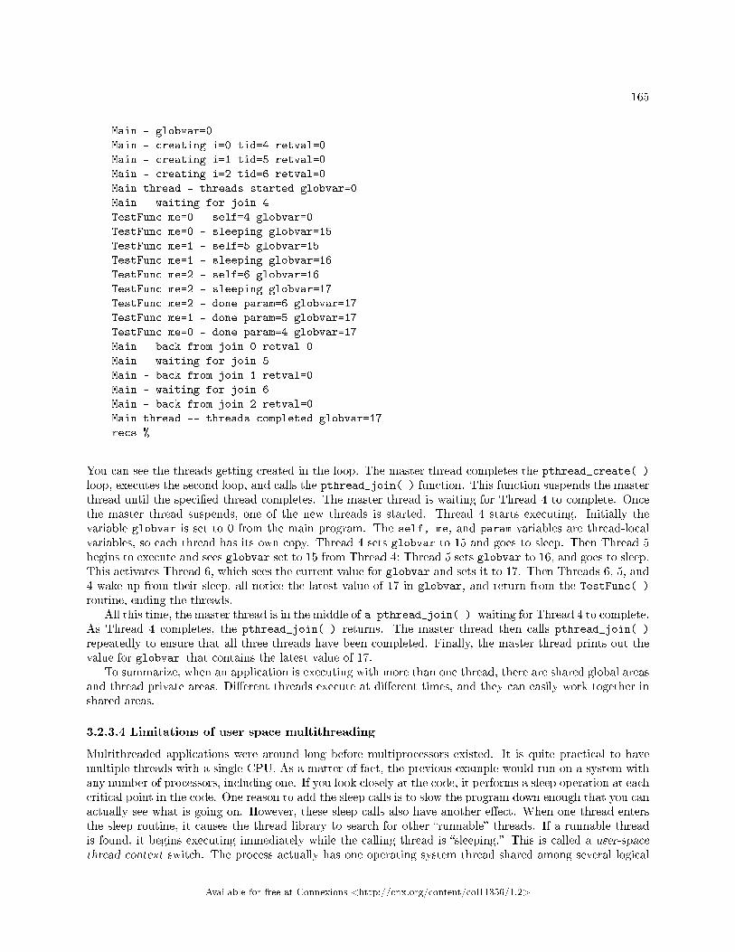
165
Main - globvar=0
Main - creating i=0 tid=4 retval=0
Main - creating i=1 tid=5 retval=0
Main - creating i=2 tid=6 retval=0
Main thread - threads started globvar=0
Main - waiting for join 4
TestFunc me=0 - self=4 globvar=0
TestFunc me=0 - sleeping globvar=15
TestFunc me=1 - self=5 globvar=15
TestFunc me=1 - sleeping globvar=16
TestFunc me=2 - self=6 globvar=16
TestFunc me=2 - sleeping globvar=17
TestFunc me=2 - done param=6 globvar=17
TestFunc me=1 - done param=5 globvar=17
TestFunc me=0 - done param=4 globvar=17
Main - back from join 0 retval=0
Main - waiting for join 5
Main - back from join 1 retval=0
Main - waiting for join 6
Main - back from join 2 retval=0
Main thread -- threads completed globvar=17
recs %
You can see the threads getting created in the loop. The master thread completes the pthread_create( )
loop, executes the second loop, and calls the pthread_join( ) function. This function suspends the masterthread until the speci�ed thread completes. The master thread is waiting for Thread 4 to complete. Oncethe master thread suspends, one of the new threads is started. Thread 4 starts executing. Initially thevariable globvar is set to 0 from the main program. The self, me, and param variables are thread-localvariables, so each thread has its own copy. Thread 4 sets globvar to 15 and goes to sleep. Then Thread 5begins to execute and sees globvar set to 15 from Thread 4; Thread 5 sets globvar to 16, and goes to sleep.This activates Thread 6, which sees the current value for globvar and sets it to 17. Then Threads 6, 5, and4 wake up from their sleep, all notice the latest value of 17 in globvar, and return from the TestFunc( )
routine, ending the threads.All this time, the master thread is in the middle of a pthread_join( ) waiting for Thread 4 to complete.
As Thread 4 completes, the pthread_join( ) returns. The master thread then calls pthread_join( )
repeatedly to ensure that all three threads have been completed. Finally, the master thread prints out thevalue for globvar that contains the latest value of 17.
To summarize, when an application is executing with more than one thread, there are shared global areasand thread private areas. Di�erent threads execute at di�erent times, and they can easily work together inshared areas.
3.2.3.4 Limitations of user space multithreading
Multithreaded applications were around long before multiprocessors existed. It is quite practical to havemultiple threads with a single CPU. As a matter of fact, the previous example would run on a system withany number of processors, including one. If you look closely at the code, it performs a sleep operation at eachcritical point in the code. One reason to add the sleep calls is to slow the program down enough that you canactually see what is going on. However, these sleep calls also have another e�ect. When one thread entersthe sleep routine, it causes the thread library to search for other �runnable� threads. If a runnable threadis found, it begins executing immediately while the calling thread is �sleeping.� This is called a user-spacethread context switch. The process actually has one operating system thread shared among several logical
Available for free at Connexions <http://cnx.org/content/col11356/1.2>
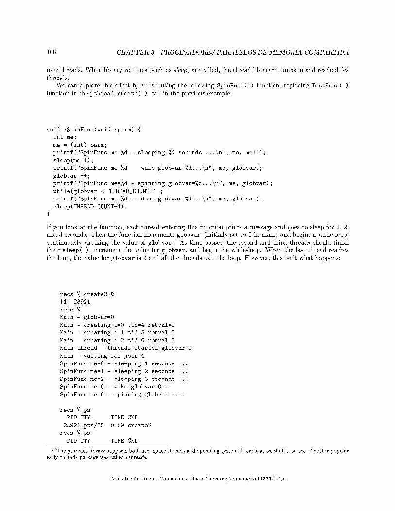
166 CHAPTER 3. PROCESADORES PARALELOS DE MEMORIA COMPARTIDA
user threads. When library routines (such as sleep) are called, the thread library18 jumps in and reschedulesthreads.
We can explore this e�ect by substituting the following SpinFunc( ) function, replacing TestFunc( )
function in the pthread_create( ) call in the previous example:
void *SpinFunc(void *parm) {
int me;
me = (int) parm;
printf("SpinFunc me=%d - sleeping %d seconds ...\n", me, me+1);
sleep(me+1);
printf("SpinFunc me=%d -- wake globvar=%d...\n", me, globvar);
globvar ++;
printf("SpinFunc me=%d - spinning globvar=%d...\n", me, globvar);
while(globvar < THREAD_COUNT ) ;
printf("SpinFunc me=%d -- done globvar=%d...\n", me, globvar);
sleep(THREAD_COUNT+1);
}
If you look at the function, each thread entering this function prints a message and goes to sleep for 1, 2,and 3 seconds. Then the function increments globvar (initially set to 0 in main) and begins a while-loop,continuously checking the value of globvar. As time passes, the second and third threads should �nishtheir sleep( ), increment the value for globvar, and begin the while-loop. When the last thread reachesthe loop, the value for globvar is 3 and all the threads exit the loop. However, this isn't what happens:
recs % create2 &
[1] 23921
recs %
Main - globvar=0
Main - creating i=0 tid=4 retval=0
Main - creating i=1 tid=5 retval=0
Main - creating i=2 tid=6 retval=0
Main thread - threads started globvar=0
Main - waiting for join 4
SpinFunc me=0 - sleeping 1 seconds ...
SpinFunc me=1 - sleeping 2 seconds ...
SpinFunc me=2 - sleeping 3 seconds ...
SpinFunc me=0 - wake globvar=0...
SpinFunc me=0 - spinning globvar=1...
recs % ps
PID TTY TIME CMD
23921 pts/35 0:09 create2
recs % ps
PID TTY TIME CMD
18The pthreads library supports both user-space threads and operating-system threads, as we shall soon see. Another popularearly threads package was called cthreads.
Available for free at Connexions <http://cnx.org/content/col11356/1.2>
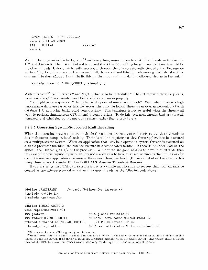
167
23921 pts/35 1:16 create2
recs % kill -9 23921
[1] Killed create2
recs %
We run the program in the background19 and everything seems to run �ne. All the threads go to sleep for1, 2, and 3 seconds. The �rst thread wakes up and starts the loop waiting for globvar to be incremented bythe other threads. Unfortunately, with user space threads, there is no automatic time sharing. Because weare in a CPU loop that never makes a system call, the second and third threads never get scheduled so theycan complete their sleep( ) call. To �x this problem, we need to make the following change to the code:
while(globvar < THREAD_COUNT ) sleep(1) ;
With this sleep20 call, Threads 2 and 3 get a chance to be �scheduled.� They then �nish their sleep calls,increment the globvar variable, and the program terminates properly.
You might ask the question, �Then what is the point of user space threads?� Well, when there is a highperformance database server or Internet server, the multiple logical threads can overlap network I/O withdatabase I/O and other background computations. This technique is not so useful when the threads allwant to perform simultaneous CPU-intensive computations. To do this, you need threads that are created,managed, and scheduled by the operating system rather than a user library.
3.2.3.5 Operating System-Supported Multithreading
When the operating system supports multiple threads per process, you can begin to use these threads todo simultaneous computational activity. There is still no requirement that these applications be executedon a multiprocessor system. When an application that uses four operating system threads is executed ona single processor machine, the threads execute in a time-shared fashion. If there is no other load on thesystem, each thread gets 1/4 of the processor. While there are good reasons to have more threads thanprocessors for noncompute applications, it's not a good idea to have more active threads than processors forcompute-intensive applications because of thread-switching overhead. (For more detail on the e�ect of toomany threads, see Appendix D, How FORTRAN Manages Threads at Runtime.
If you are using the POSIX threads library, it is a simple modi�cation to request that your threads becreated as operating-system rather rather than user threads, as the following code shows:
#define _REENTRANT /* basic 3-lines for threads */
#include <stdio.h>#include <pthread.h>
#define THREAD_COUNT 2
void *SpinFunc(void *);
int globvar; /* A global variable */
int index[THREAD_COUNT]; /* Local zero-based thread index */
pthread_t thread_id[THREAD_COUNT]; /* POSIX Thread IDs */
pthread_attr_t attr; /* Thread attributes NULL=use default */
19Because we know it will hang and ignore interrupts.20Some thread libraries support a call to a routine sched_yield( ) that checks for runnable threads. If it �nds a runnable
thread, it runs the thread. If no thread is runnable, it returns immediately to the calling thread. This routine allows a threadthat has the CPU to ensure that other threads make progress during CPU-intensive periods of its code.
Available for free at Connexions <http://cnx.org/content/col11356/1.2>
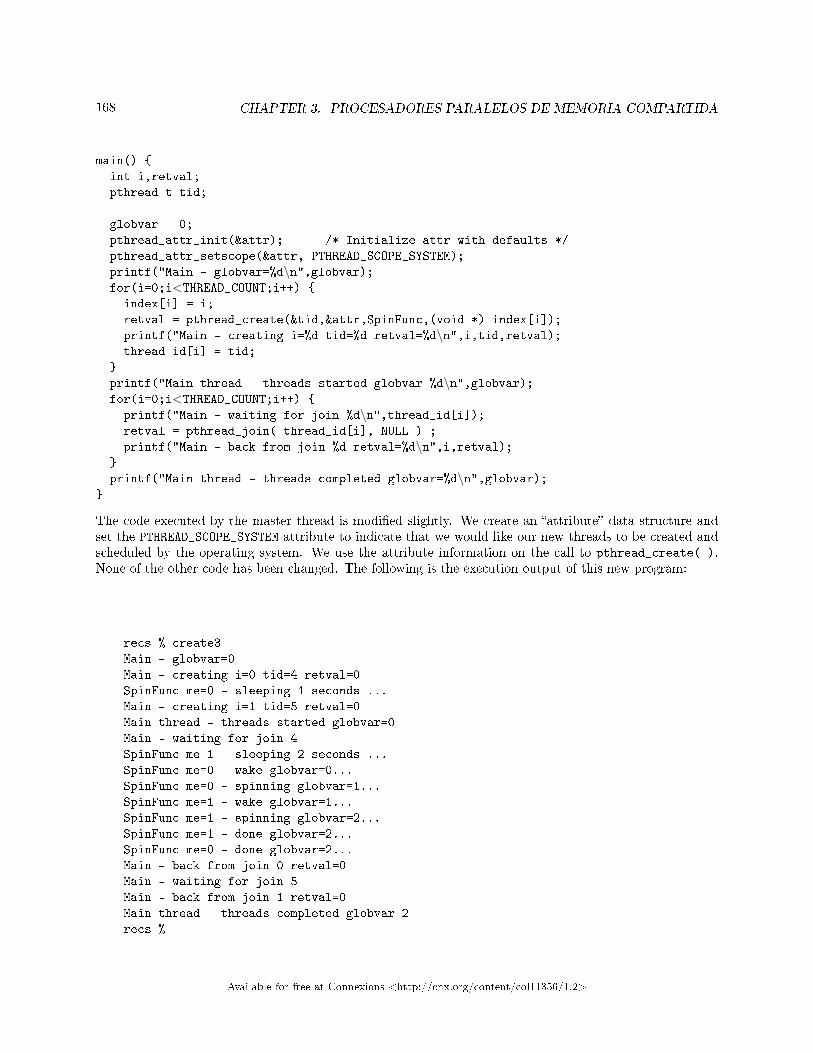
168 CHAPTER 3. PROCESADORES PARALELOS DE MEMORIA COMPARTIDA
main() {
int i,retval;
pthread_t tid;
globvar = 0;
pthread_attr_init(&attr); /* Initialize attr with defaults */
pthread_attr_setscope(&attr, PTHREAD_SCOPE_SYSTEM);
printf("Main - globvar=%d\n",globvar);for(i=0;i<THREAD_COUNT;i++) {
index[i] = i;
retval = pthread_create(&tid,&attr,SpinFunc,(void *) index[i]);
printf("Main - creating i=%d tid=%d retval=%d\n",i,tid,retval);thread_id[i] = tid;
}
printf("Main thread - threads started globvar=%d\n",globvar);for(i=0;i<THREAD_COUNT;i++) {
printf("Main - waiting for join %d\n",thread_id[i]);retval = pthread_join( thread_id[i], NULL ) ;
printf("Main - back from join %d retval=%d\n",i,retval);}
printf("Main thread - threads completed globvar=%d\n",globvar);}
The code executed by the master thread is modi�ed slightly. We create an �attribute� data structure andset the PTHREAD_SCOPE_SYSTEM attribute to indicate that we would like our new threads to be created andscheduled by the operating system. We use the attribute information on the call to pthread_create( ).None of the other code has been changed. The following is the execution output of this new program:
recs % create3
Main - globvar=0
Main - creating i=0 tid=4 retval=0
SpinFunc me=0 - sleeping 1 seconds ...
Main - creating i=1 tid=5 retval=0
Main thread - threads started globvar=0
Main - waiting for join 4
SpinFunc me=1 - sleeping 2 seconds ...
SpinFunc me=0 - wake globvar=0...
SpinFunc me=0 - spinning globvar=1...
SpinFunc me=1 - wake globvar=1...
SpinFunc me=1 - spinning globvar=2...
SpinFunc me=1 - done globvar=2...
SpinFunc me=0 - done globvar=2...
Main - back from join 0 retval=0
Main - waiting for join 5
Main - back from join 1 retval=0
Main thread - threads completed globvar=2
recs %
Available for free at Connexions <http://cnx.org/content/col11356/1.2>
169
Now the program executes properly. When the �rst thread starts spinning, the operating system is contextswitching between all three threads. As the threads come out of their sleep( ), they increment their sharedvariable, and when the �nal thread increments the shared variable, the other two threads instantly noticethe new value (because of the cache coherency protocol) and �nish the loop. If there are fewer than threeCPUs, a thread may have to wait for a time-sharing context switch to occur before it notices the updatedglobal variable.
With operating-system threads and multiple processors, a program can realistically break up a largecomputation between several independent threads and compute the solution more quickly. Of course thispresupposes that the computation could be done in parallel in the �rst place.
3.2.4 Techniques for Multithreaded Programs21
Given that we have multithreaded capabilities and multiprocessors, we must still convince the threads towork together to accomplish some overall goal. Often we need some ways to coordinate and cooperatebetween the threads. There are several important techniques that are used while the program is runningwith multiple threads, including:
• Fork-join (or create-join) programming• Synchronization using a critical section with a lock, semaphore, or mutex• Barriers
Each of these techniques has an overhead associated with it. Because these overheads are necessary to goparallel, we must make sure that we have su�cient work to make the bene�t of parallel operation worth thecost.
3.2.4.1 Fork-Join Programming
This approach is the simplest method of coordinating your threads. As in the earlier examples in this chapter,a master thread sets up some global data structures that describe the tasks each thread is to perform andthen use the pthread_create( ) function to activate the proper number of threads. Each thread checksthe global data structure using its thread-id as an index to �nd its task. The thread then performs the taskand completes. The master thread waits at a pthread_join( ) point, and when a thread has completed,it updates the global data structure and creates a new thread. These steps are repeated for each majoriteration (such as a time-step) for the duration of the program:
for(ts=0;ts<10000;ts++) { /* Time Step Loop */
/* Setup tasks */
for (ith=0;ith<NUM_THREADS;ith++) pthread_create(..,work_routine,..)
for (ith=0;ith<NUM_THREADS;ith++) pthread_join(...)
}
work_routine() {
/* Perform Task */
return;
}
The shortcoming of this approach is the overhead cost associated with creating and destroying an operatingsystem thread for a potentially very short task.
The other approach is to have the threads created at the beginning of the program and to have themcommunicate amongst themselves throughout the duration of the application. To do this, they use suchtechniques as critical sections or barriers.
21This content is available online at <http://cnx.org/content/m32802/1.3/>.
Available for free at Connexions <http://cnx.org/content/col11356/1.2>
170 CHAPTER 3. PROCESADORES PARALELOS DE MEMORIA COMPARTIDA
3.2.4.2 Synchronization
Synchronization is needed when there is a particular operation to a shared variable that can only be performedby one processor at a time. For example, in previous SpinFunc( ) examples, consider the line:
globvar++;
In assembly language, this takes at least three instructions:
LOAD R1,globvar
ADD R1,1
STORE R1,globvar
What if globvar contained 0, Thread 1 was running, and, at the precise moment it completed the LOAD intoRegister R1 and before it had completed the ADD or STORE instructions, the operating system interrupted thethread and switched to Thread 2? Thread 2 catches up and executes all three instructions using its registers:loading 0, adding 1 and storing the 1 back into globvar. Now Thread 2 goes to sleep and Thread 1 isrestarted at the ADD instruction. Register R1 for Thread 1 contains the previously loaded value of 0; Thread1 adds 1 and then stores 1 into globvar. What is wrong with this picture? We meant to use this code tocount the number of threads that have passed this point. Two threads passed the point, but because of abad case of bad timing, our variable indicates only that one thread passed. This is because the increment ofa variable in memory is not atomic. That is, halfway through the increment, something else can happen.
Another way we can have a problem is on a multiprocessor when two processors execute these instructionssimultaneously. They both do the LOAD, getting 0. Then they both add 1 and store 1 back to memory.22
Which processor actually got the honor of storing their 1 back to memory is simply a race.We must have some way of guaranteeing that only one thread can be in these three instructions at the
same time. If one thread has started these instructions, all other threads must wait to enter until the �rstthread has exited. These areas are called critical sections. On single-CPU systems, there was a simplesolution to critical sections: you could turn o� interrupts for a few instructions and then turn them backon. This way you could guarantee that you would get all the way through before a timer or other interruptoccurred:
INTOFF // Turn off Interrupts
LOAD R1,globvar
ADD R1,1
STORE R1,globvar
INTON // Turn on Interrupts
However, this technique does not work for longer critical sections or when there is more than one CPU. Inthese cases, you need a lock, a semaphore, or a mutex. Most thread libraries provide this type of routine.To use a mutex, we have to make some modi�cations to our example code:
22Boy, this is getting pretty picky. How often will either of these events really happen? Well, if it crashes your airlinereservation system every 100,000 transactions or so, that would be way too often.
Available for free at Connexions <http://cnx.org/content/col11356/1.2>
171
...
pthread_mutex_t my_mutex; /* MUTEX data structure */
...
main() {
...
pthread_attr_init(&attr); /* Initialize attr with defaults */
pthread_mutex_init (&my_mutex, NULL);
.... pthread_create( ... )
...
}
void *SpinFunc(void *parm) {
...
pthread_mutex_lock (&my_mutex);
globvar ++;
pthread_mutex_unlock (&my_mutex);
while(globvar < THREAD_COUNT ) ;
printf("SpinFunc me=%d -- done globvar=%d...\n", me, globvar);
...
}
The mutex data structure must be declared in the shared area of the program. Before the threads arecreated, pthread_mutex_init must be called to initialize the mutex. Before globvar is incremented, wemust lock the mutex and after we �nish updating globvar (three instructions later), we unlock the mutex.With the code as shown above, there will never be more than one processor executing the globvar++ lineof code, and the code will never hang because an increment was missed. Semaphores and locks are used ina similar way.
Interestingly, when using user space threads, an attempt to lock an already locked mutex, semaphore, orlock can cause a thread context switch. This allows the thread that �owns� the lock a better chance to makeprogress toward the point where they will unlock the critical section. Also, the act of unlocking a mutex cancause the thread waiting for the mutex to be dispatched by the thread library.
3.2.4.3 Barriers
Barriers are di�erent than critical sections. Sometimes in a multithreaded application, you need to have allthreads arrive at a point before allowing any threads to execute beyond that point. An example of this isa time-based simulation. Each task processes its portion of the simulation but must wait until all of thethreads have completed the current time step before any thread can begin the next time step. Typicallythreads are created, and then each thread executes a loop with one or more barriers in the loop. The roughpseudocode for this type of approach is as follows:
main() {
for (ith=0;ith<NUM_THREADS;ith++) pthread_create(..,work_routine,..)
for (ith=0;ith<NUM_THREADS;ith++) pthread_join(...) /* Wait a long time */
exit()
}
work_routine() {
for(ts=0;ts<10000;ts++) { /* Time Step Loop */
/* Compute total forces on particles */
wait_barrier();
/* Update particle positions based on the forces */
Available for free at Connexions <http://cnx.org/content/col11356/1.2>
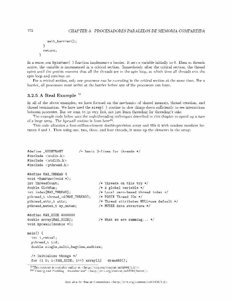
172 CHAPTER 3. PROCESADORES PARALELOS DE MEMORIA COMPARTIDA
wait_barrier();
}
return;
}
In a sense, our SpinFunc( ) function implements a barrier. It sets a variable initially to 0. Then as threadsarrive, the variable is incremented in a critical section. Immediately after the critical section, the threadspins until the precise moment that all the threads are in the spin loop, at which time all threads exit thespin loop and continue on.
For a critical section, only one processor can be executing in the critical section at the same time. For abarrier, all processors must arrive at the barrier before any of the processors can leave.
3.2.5 A Real Example 23
In all of the above examples, we have focused on the mechanics of shared memory, thread creation, andthread termination. We have used the sleep( ) routine to slow things down su�ciently to see interactionsbetween processes. But we want to go very fast, not just learn threading for threading's sake.
The example code below uses the multithreading techniques described in this chapter to speed up a sumof a large array. The hpcwall routine is from here24.
This code allocates a four-million-element double-precision array and �lls it with random numbers be-tween 0 and 1. Then using one, two, three, and four threads, it sums up the elements in the array:
#define _REENTRANT /* basic 3-lines for threads */
#include <stdio.h>#include <stdlib.h>#include <pthread.h>
#define MAX_THREAD 4
void *SumFunc(void *);
int ThreadCount; /* Threads on this try */
double GlobSum; /* A global variable */
int index[MAX_THREAD]; /* Local zero-based thread index */
pthread_t thread_id[MAX_THREAD]; /* POSIX Thread IDs */
pthread_attr_t attr; /* Thread attributes NULL=use default */
pthread_mutex_t my_mutex; /* MUTEX data structure */
#define MAX_SIZE 4000000
double array[MAX_SIZE]; /* What we are summing... */
void hpcwall(double *);
main() {
int i,retval;
pthread_t tid;
double single,multi,begtime,endtime;
/* Initialize things */
for (i=0; i<MAX_SIZE; i++) array[i] = drand48();
23This content is available online at <http://cnx.org/content/m32804/1.3/>.24"Timing and Pro�ling - Introduction" <http://cnx.org/content/m33704/latest/>
Available for free at Connexions <http://cnx.org/content/col11356/1.2>

173
pthread_attr_init(&attr); /* Initialize attr with defaults */
pthread_mutex_init (&my_mutex, NULL);
pthread_attr_setscope(&attr, PTHREAD_SCOPE_SYSTEM);
/* Single threaded sum */
GlobSum = 0;
hpcwall(&begtime);
for(i=0; i<MAX_SIZE;i++) GlobSum = GlobSum + array[i];
hpcwall(&endtime);
single = endtime - begtime;
printf("Single sum=%lf time=%lf\n",GlobSum,single);
/* Use different numbers of threads to accomplish the same thing */
for(ThreadCount=2;ThreadCount<=MAX_THREAD; ThreadCount++) {
printf("Threads=%d\n",ThreadCount);GlobSum = 0;
hpcwall(&begtime);
for(i=0;i<ThreadCount;i++) {
index[i] = i;
retval = pthread_create(&tid,&attr,SumFunc,(void *) index[i]);
thread_id[i] = tid;
}
for(i=0;i<ThreadCount;i++) retval = pthread_join(thread_id[i],NULL);
hpcwall(&endtime);
multi = endtime - begtime;
printf("Sum=%lf time=%lf\n",GlobSum,multi);printf("Efficiency = %lf\n",single/(multi*ThreadCount));
} /* End of the ThreadCount loop */
}
void *SumFunc(void *parm){
int i,me,chunk,start,end;
double LocSum;
/* Decide which iterations belong to me */
me = (int) parm;
chunk = MAX_SIZE / ThreadCount;
start = me * chunk;
end = start + chunk; /* C-Style - actual element + 1 */
if ( me == (ThreadCount-1) ) end = MAX_SIZE;
printf("SumFunc me=%d start=%d end=%d\n",me,start,end);
/* Compute sum of our subset*/
LocSum = 0;
for(i=start;i<end;i++ ) LocSum = LocSum + array[i];
/* Update the global sum and return to the waiting join */
pthread_mutex_lock (&my_mutex);
GlobSum = GlobSum + LocSum;
pthread_mutex_unlock (&my_mutex);
}
Available for free at Connexions <http://cnx.org/content/col11356/1.2>
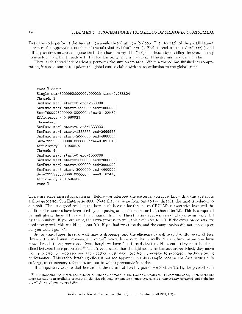
174 CHAPTER 3. PROCESADORES PARALELOS DE MEMORIA COMPARTIDA
First, the code performs the sum using a single thread using a for-loop. Then for each of the parallel sums,it creates the appropriate number of threads that call SumFunc( ). Each thread starts in SumFunc( ) andinitially chooses an area to operation in the shared array. The �strip� is chosen by dividing the overall arrayup evenly among the threads with the last thread getting a few extra if the division has a remainder.
Then, each thread independently performs the sum on its area. When a thread has �nished its compu-tation, it uses a mutex to update the global sum variable with its contribution to the global sum:
recs % addup
Single sum=7999998000000.000000 time=0.256624
Threads=2
SumFunc me=0 start=0 end=2000000
SumFunc me=1 start=2000000 end=4000000
Sum=7999998000000.000000 time=0.133530
Efficiency = 0.960923
Threads=3
SumFunc me=0 start=0 end=1333333
SumFunc me=1 start=1333333 end=2666666
SumFunc me=2 start=2666666 end=4000000
Sum=7999998000000.000000 time=0.091018
Efficiency = 0.939829
Threads=4
SumFunc me=0 start=0 end=1000000
SumFunc me=1 start=1000000 end=2000000
SumFunc me=2 start=2000000 end=3000000
SumFunc me=3 start=3000000 end=4000000
Sum=7999998000000.000000 time=0.107473
Efficiency = 0.596950
recs %
There are some interesting patterns. Before you interpret the patterns, you must know that this system isa three-processor Sun Enterprise 3000. Note that as we go from one to two threads, the time is reduced toone-half. That is a good result given how much it costs for that extra CPU. We characterize how well theadditional resources have been used by computing an e�ciency factor that should be 1.0. This is computedby multiplying the wall time by the number of threads. Then the time it takes on a single processor is dividedby this number. If you are using the extra processors well, this evaluates to 1.0. If the extra processors areused pretty well, this would be about 0.9. If you had two threads, and the computation did not speed up atall, you would get 0.5.
At two and three threads, wall time is dropping, and the e�ciency is well over 0.9. However, at fourthreads, the wall time increases, and our e�ciency drops very dramatically. This is because we now havemore threads than processors. Even though we have four threads that could execute, they must be time-sliced between three processors.25 This is even worse that it might seem. As threads are switched, they movefrom processor to processor and their caches must also move from processor to processor, further slowingperformance. This cache-thrashing e�ect is not too apparent in this example because the data structure isso large, most memory references are not to values previously in cache.
It's important to note that because of the nature of �oating-point (see Section 1.2.1), the parallel sum
25It is important to match the number of runnable threads to the available resources. In compute code, when there aremore threads than available processors, the threads compete among themselves, causing unnecessary overhead and reducingthe e�ciency of your computation.
Available for free at Connexions <http://cnx.org/content/col11356/1.2>
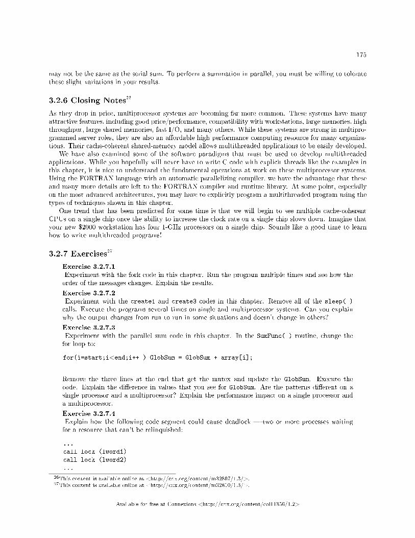
175
may not be the same as the serial sum. To perform a summation in parallel, you must be willing to toleratethese slight variations in your results.
3.2.6 Closing Notes26
As they drop in price, multiprocessor systems are becoming far more common. These systems have manyattractive features, including good price/performance, compatibility with workstations, large memories, highthroughput, large shared memories, fast I/O, and many others. While these systems are strong in multipro-grammed server roles, they are also an a�ordable high performance computing resource for many organiza-tions. Their cache-coherent shared-memory model allows multithreaded applications to be easily developed.
We have also examined some of the software paradigms that must be used to develop multithreadedapplications. While you hopefully will never have to write C code with explicit threads like the examples inthis chapter, it is nice to understand the fundamental operations at work on these multiprocessor systems.Using the FORTRAN language with an automatic parallelizing compiler, we have the advantage that theseand many more details are left to the FORTRAN compiler and runtime library. At some point, especiallyon the most advanced architectures, you may have to explicitly program a multithreaded program using thetypes of techniques shown in this chapter.
One trend that has been predicted for some time is that we will begin to see multiple cache-coherentCPUs on a single chip once the ability to increase the clock rate on a single chip slows down. Imagine thatyour new $2000 workstation has four 1-GHz processors on a single chip. Sounds like a good time to learnhow to write multithreaded programs!
3.2.7 Exercises27
Exercise 3.2.7.1Experiment with the fork code in this chapter. Run the program multiple times and see how theorder of the messages changes. Explain the results.
Exercise 3.2.7.2Experiment with the create1 and create3 codes in this chapter. Remove all of the sleep( )
calls. Execute the programs several times on single and multiprocessor systems. Can you explainwhy the output changes from run to run in some situations and doesn't change in others?
Exercise 3.2.7.3Experiment with the parallel sum code in this chapter. In the SumFunc( ) routine, change thefor-loop to:
for(i=start;i<end;i++ ) GlobSum = GlobSum + array[i];
Remove the three lines at the end that get the mutex and update the GlobSum. Execute thecode. Explain the di�erence in values that you see for GlobSum. Are the patterns di�erent on asingle processor and a multiprocessor? Explain the performance impact on a single processor anda multiprocessor.
Exercise 3.2.7.4Explain how the following code segment could cause deadlock � two or more processes waitingfor a resource that can't be relinquished:
...
call lock (lword1)
call lock (lword2)
...
26This content is available online at <http://cnx.org/content/m32807/1.3/>.27This content is available online at <http://cnx.org/content/m32810/1.3/>.
Available for free at Connexions <http://cnx.org/content/col11356/1.2>
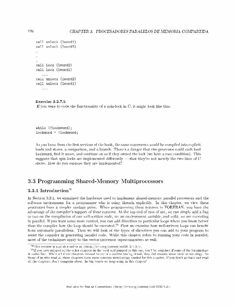
176 CHAPTER 3. PROCESADORES PARALELOS DE MEMORIA COMPARTIDA
call unlock (lword1)
call unlock (lword2)
.
.
.
call lock (lword2)
call lock (lword1)
...
call unlock (lword2)
call unlock (lword1)
...
Exercise 3.2.7.5If you were to code the functionality of a spin-lock in C, it might look like this:
while (!lockword);
lockword = !lockword;
As you know from the �rst sections of the book, the same statements would be compiled into explicitloads and stores, a comparison, and a branch. There's a danger that two processes could each loadlockword, �nd it unset, and continue on as if they owned the lock (we have a race condition). Thissuggests that spin-locks are implemented di�erently � that they're not merely the two lines of Cabove. How do you suppose they are implemented?
3.3 Programming Shared-Memory Multiprocessors
3.3.1 Introduction28
In Section 3.2.1, we examined the hardware used to implement shared-memory parallel processors and thesoftware environment for a programmer who is using threads explicitly. In this chapter, we view theseprocessors from a simpler vantage point. When programming these systems in FORTRAN, you have theadvantage of the compiler's support of these systems. At the top end of ease of use, we can simply add a �agor two on the compilation of our well-written code, set an environment variable, and voilá, we are executingin parallel. If you want some more control, you can add directives to particular loops where you know betterthan the compiler how the loop should be executed.29 First we examine how well-written loops can bene�tfrom automatic parallelism. Then we will look at the types of directives you can add to your program toassist the compiler in generating parallel code. While this chapter refers to running your code in parallel,most of the techniques apply to the vector-processor supercomputers as well.
28This content is available online at <http://cnx.org/content/m32812/1.3/>.29If you have skipped all the other chapters in the book and jumped to this one, don't be surprised if some of the terminology
is unfamiliar. While all those chapters seemed to contain endless boring detail, they did contain some basic terminology. Sothose of us who read all those chapters have some common terminology needed for this chapter. If you don't go back and readall the chapters, don't complain about the big words we keep using in this chapter!
Available for free at Connexions <http://cnx.org/content/col11356/1.2>
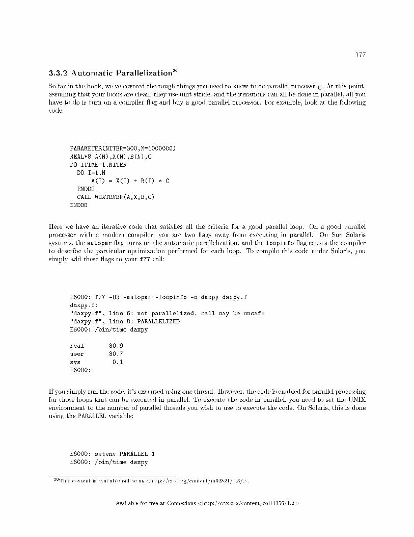
177
3.3.2 Automatic Parallelization30
So far in the book, we've covered the tough things you need to know to do parallel processing. At this point,assuming that your loops are clean, they use unit stride, and the iterations can all be done in parallel, all youhave to do is turn on a compiler �ag and buy a good parallel processor. For example, look at the followingcode:
PARAMETER(NITER=300,N=1000000)
REAL*8 A(N),X(N),B(N),C
DO ITIME=1,NITER
DO I=1,N
A(I) = X(I) + B(I) * C
ENDDO
CALL WHATEVER(A,X,B,C)
ENDDO
Here we have an iterative code that satis�es all the criteria for a good parallel loop. On a good parallelprocessor with a modern compiler, you are two �ags away from executing in parallel. On Sun Solarissystems, the autopar �ag turns on the automatic parallelization, and the loopinfo �ag causes the compilerto describe the particular optimization performed for each loop. To compile this code under Solaris, yousimply add these �ags to your f77 call:
E6000: f77 -O3 -autopar -loopinfo -o daxpy daxpy.f
daxpy.f:
"daxpy.f", line 6: not parallelized, call may be unsafe
"daxpy.f", line 8: PARALLELIZED
E6000: /bin/time daxpy
real 30.9
user 30.7
sys 0.1
E6000:
If you simply run the code, it's executed using one thread. However, the code is enabled for parallel processingfor those loops that can be executed in parallel. To execute the code in parallel, you need to set the UNIXenvironment to the number of parallel threads you wish to use to execute the code. On Solaris, this is doneusing the PARALLEL variable:
E6000: setenv PARALLEL 1
E6000: /bin/time daxpy
30This content is available online at <http://cnx.org/content/m32821/1.3/>.
Available for free at Connexions <http://cnx.org/content/col11356/1.2>
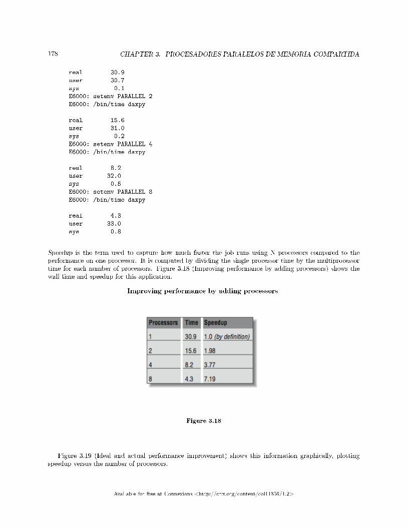
178 CHAPTER 3. PROCESADORES PARALELOS DE MEMORIA COMPARTIDA
real 30.9
user 30.7
sys 0.1
E6000: setenv PARALLEL 2
E6000: /bin/time daxpy
real 15.6
user 31.0
sys 0.2
E6000: setenv PARALLEL 4
E6000: /bin/time daxpy
real 8.2
user 32.0
sys 0.5
E6000: setenv PARALLEL 8
E6000: /bin/time daxpy
real 4.3
user 33.0
sys 0.8
Speedup is the term used to capture how much faster the job runs using N processors compared to theperformance on one processor. It is computed by dividing the single processor time by the multiprocessortime for each number of processors. Figure 3.18 (Improving performance by adding processors) shows thewall time and speedup for this application.
Improving performance by adding processors
Figure 3.18
Figure 3.19 (Ideal and actual performance improvement) shows this information graphically, plottingspeedup versus the number of processors.
Available for free at Connexions <http://cnx.org/content/col11356/1.2>
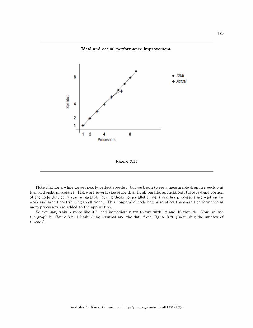
179
Ideal and actual performance improvement
Figure 3.19
Note that for a while we get nearly perfect speedup, but we begin to see a measurable drop in speedup atfour and eight processors. There are several causes for this. In all parallel applications, there is some portionof the code that can't run in parallel. During those nonparallel times, the other processors are waiting forwork and aren't contributing to e�ciency. This nonparallel code begins to a�ect the overall performance asmore processors are added to the application.
So you say, �this is more like it!� and immediately try to run with 12 and 16 threads. Now, we seethe graph in Figure 3.21 (Diminishing returns) and the data from Figure 3.20 (Increasing the number ofthreads).
Available for free at Connexions <http://cnx.org/content/col11356/1.2>
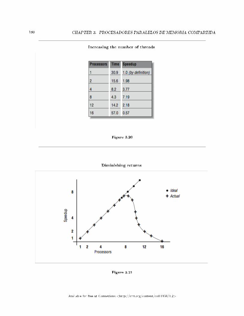
180 CHAPTER 3. PROCESADORES PARALELOS DE MEMORIA COMPARTIDA
Increasing the number of threads
Figure 3.20
Diminishing returns
Figure 3.21
Available for free at Connexions <http://cnx.org/content/col11356/1.2>
181
What has happened here? Things were going so well, and then they slowed down. We are running thisprogram on a 16-processor system, and there are eight other active threads, as indicated below:
E6000:uptime
4:00pm up 19 day(s), 37 min(s), 5 users, load average: 8.00, 8.05, 8.14
E6000:
Once we pass eight threads, there are no available processors for our threads. So the threads must be time-shared between the processors, signi�cantly slowing the overall operation. By the end, we are executing 16threads on eight processors, and our performance is slower than with one thread. So it is important thatyou don't create too many threads in these types of applications.
3.3.2.1 Compiler Considerations
Improving performance by turning on automatic parallelization is an example of the �smarter compiler� wediscussed in earlier chapters. The addition of a single compiler �ag has triggered a great deal of analysis onthe part of the compiler including:
• Which loops can execute in parallel, producing the exact same results as the sequential executions ofthe loops? This is done by checking for dependencies that span iterations. A loop with no interiterationdependencies is called a DOALL loop.
• Which loops are worth executing in parallel? Generally very short loops gain no bene�t and mayexecute more slowly when executing in parallel. As with loop unrolling, parallelism always has a cost.It is best used when the bene�t far outweighs the cost.
• In a loop nest, which loop is the best candidate to be parallelized? Generally the best performanceoccurs when we parallelize the outermost loop of a loop nest. This way the overhead associated withbeginning a parallel loop is amortized over a longer parallel loop duration.
• Can and should the loop nest be interchanged? The compiler may detect that the loops in a nestcan be done in any order. One order may work very well for parallel code while giving poor memoryperformance. Another order may give unit stride but perform poorly with multiple threads. Thecompiler must analyze the cost/bene�t of each approach and make the best choice.
• How do we break up the iterations among the threads executing a parallel loop? Are the iterationsshort with uniform duration, or long with wide variation of execution time? We will see that thereare a number of di�erent ways to accomplish this. When the programmer has given no guidance, thecompiler must make an educated guess.
Even though it seems complicated, the compiler can do a surprisingly good job on a wide variety of codes.It is not magic, however. For example, in the following code we have a loop-carried �ow dependency:
PROGRAM DEP
PARAMETER(NITER=300,N=1000000)
REAL*4 A(N)
DO ITIME=1,NITER
CALL WHATEVER(A)
DO I=2,N
Available for free at Connexions <http://cnx.org/content/col11356/1.2>
182 CHAPTER 3. PROCESADORES PARALELOS DE MEMORIA COMPARTIDA
A(I) = A(I-1) + A(I) * C
ENDDO
ENDDO
END
When we compile the code, the compiler gives us the following message:
E6000: f77 -O3 -autopar -loopinfo -o dep dep.f
dep.f:
"dep.f", line 6: not parallelized, call may be unsafe
"dep.f", line 8: not parallelized, unsafe dependence (a)
E6000:
The compiler throws its hands up in despair, and lets you know that the loop at Line 8 had an unsafedependence, and so it won't automatically parallelize the loop. When the code is executed below, adding athread does not a�ect the execution performance:
E6000:setenv PARALLEL 1
E6000:/bin/time dep
real 18.1
user 18.1
sys 0.0
E6000:setenv PARALLEL 2
E6000:/bin/time dep
real 18.3
user 18.2
sys 0.0
E6000:
A typical application has many loops. Not all the loops are executed in parallel. It's a good idea to run apro�le of your application, and in the routines that use most of the CPU time, check to �nd out which loopsare not being parallelized. Within a loop nest, the compiler generally chooses only one loop to execute inparallel.
3.3.2.2 Other Compiler Flags
In addition to the �ags shown above, you may have other compiler �ags available to you that apply acrossthe entire program:
• You may have a compiler �ag to enable the automatic parallelization of reduction operations. Becausethe order of additions can a�ect the �nal value when computing a sum of �oating-point numbers, thecompiler needs permission to parallelize summation loops.
Available for free at Connexions <http://cnx.org/content/col11356/1.2>

183
• Flags that relax the compliance with IEEE �oating-point rules may also give the compiler more �ex-ibility when trying to parallelize a loop. However, you must be sure that it's not causing accuracyproblems in other areas of your code.
• Often a compiler has a �ag called �unsafe optimization� or �assume no dependencies.� While this �agmay indeed enhance the performance of an application with loops that have dependencies, it almostcertainly produces incorrect results.
There is some value in experimenting with a compiler to see the particular combination that will yield goodperformance across a variety of applications. Then that set of compiler options can be used as a startingpoint when you encounter a new application.
3.3.3 Assisting the Compiler31
If it were all that simple, you wouldn't need this book. While compilers are extremely clever, there is still alot of ways to improve the performance of your code without sacri�cing its portability. Instead of convertingthe whole program to C and using a thread library, you can assist the compiler by adding compiler directivesto our source code.
Compiler directives are typically inserted in the form of stylized FORTRAN comments. This is doneso that a nonparallelizing compiler can ignore them and just look at the FORTRAN code, sans comments.This allows to you tune your code for parallel architectures without letting it run badly on a wide range ofsingle-processor systems.
There are two categories of parallel-processing comments:
• Assertions• Manual parallelization directives
Assertions tell the compiler certain things that you as the programmer know about the code that it mightnot guess by looking at the code. Through the assertions, you are attempting to assuage the compiler'sdoubts about whether or not the loop is eligible for parallelization. When you use directives, you are takingfull responsibility for the correct execution of the program. You are telling the compiler what to parallelizeand how to do it. You take full responsibility for the output of the program. If the program producesmeaningless results, you have no one to blame but yourself.
3.3.3.1 Assertions
In a previous example, we compiled a program and received the following output:
E6000: f77 -O3 -autopar -loopinfo -o dep dep.f
dep.f:
"dep.f", line 6: not parallelized, call may be unsafe
"dep.f", line 8: not parallelized, unsafe dependence (a)
E6000:
An uneducated programmer who has not read this book (or has not looked at the code) might exclaim, �Whatunsafe dependence, I never put one of those in my code!� and quickly add a no dependencies assertion. Thisis the essence of an assertion. Instead of telling the compiler to simply parallelize the loop, the programmeris telling the compiler that its conclusion that there is a dependence is incorrect. Usually the net result isthat the compiler does indeed parallelize the loop.
We will brie�y review the types of assertions that are typically supported by these compilers. An assertionis generally added to the code using a stylized comment.
31This content is available online at <http://cnx.org/content/m32814/1.3/>.
Available for free at Connexions <http://cnx.org/content/col11356/1.2>
184 CHAPTER 3. PROCESADORES PARALELOS DE MEMORIA COMPARTIDA
3.3.3.1.1 No dependencies
A no dependencies or ignore dependencies directive tells the compiler that references don't overlap.That is, it tells the compiler to generate code that may execute incorrectly if there are dependencies. You'resaying, �I know what I'm doing; it's OK to overlap references.� A no dependencies directive might help thefollowing loop:
DO I=1,N
A(I) = A(I+K) * B(I)
ENDDO
If you know that k is greater than -1 or less than -n, you can get the compiler to parallelize the loop:
C$ASSERT NO_DEPENDENCIES
DO I=1,N
A(I) = A(I+K) * B(I)
ENDDO
Of course, blindly telling the compiler that there are no dependencies is a prescription for disaster. If k
equals -1, the example above becomes a recursive loop.
3.3.3.1.2 Relations
You will often see loops that contain some potential dependencies, making them bad candidates for a nodependencies directive. However, you may be able to supply some local facts about certain variables. Thisallows partial parallelization without compromising the results. In the code below, there are two potentialdependencies because of subscripts involving k and j:
for (i=0; i<n; i++) {
a[i] = a[i+k] * b[i];
c[i] = c[i+j] * b[i];
}
Perhaps we know that there are no con�icts with references to a[i] and a[i+k]. But maybe we aren't sosure about c[i] and c[i+j]. Therefore, we can't say in general that there are no dependencies. However, wemay be able to say something explicit about k (like �k is always greater than -1�), leaving j out of it. Thisinformation about the relationship of one expression to another is called a relation assertion. Applying arelation assertion allows the compiler to apply its optimization to the �rst statement in the loop, giving uspartial parallelization.32
Again, if you supply inaccurate testimony that leads the compiler to make unsafe optimizations, youranswer may be wrong.
32Notice that, if you were tuning by hand, you could split this loop into two: one parallelizable and one not.
Available for free at Connexions <http://cnx.org/content/col11356/1.2>
185
3.3.3.1.3 Permutations
As we have seen elsewhere, when elements of an array are indirectly addressed, you have to worry aboutwhether or not some of the subscripts may be repeated. In the code below, are the values of K(I) all unique?Or are there duplicates?
DO I=1,N
A(K(I)) = A(K(I)) + B(I) * C
END DO
If you know there are no duplicates in K (i.e., that A(K(I)) is a permutation), you can inform the compilerso that iterations can execute in parallel. You supply the information using a permutation assertion.
3.3.3.1.4 No equivalences
Equivalenced arrays in FORTRAN programs provide another challenge for the compiler. If any elements oftwo equivalenced arrays appear in the same loop, most compilers assume that references could point to thesame memory storage location and optimize very conservatively. This may be true even if it is abundantlyapparent to you that there is no overlap whatsoever.
You inform the compiler that references to equivalenced arrays are safe with a no equivalences assertion.Of course, if you don't use equivalences, this assertion has no e�ect.
3.3.3.1.5 Trip count
Each loop can be characterized by an average number of iterations. Some loops are never executed or goaround just a few times. Others may go around hundreds of times:
C$ASSERT TRIPCOUNT>100
DO I=L,N
A(I) = B(I) + C(I)
END DO
Your compiler is going to look at every loop as a candidate for unrolling or parallelization. It's working inthe dark, however, because it can't tell which loops are important and tries to optimize them all. This canlead to the surprising experience of seeing your runtime go up after optimization!
A trip count assertion provides a clue to the compiler that helps it decide how much to unroll a loopor when to parallelize a loop.33 Loops that aren't important can be identi�ed with low or zero trip counts.Important loops have high trip counts.
3.3.3.1.6 Inline substitution
If your compiler supports procedure inlining, you can use directives and command-line switches to specifyhow many nested levels of procedures you would like to inline, thresholds for procedure size, etc. The vendorwill have chosen reasonable defaults.
33The assertion is made either by hand or from a pro�ler.
Available for free at Connexions <http://cnx.org/content/col11356/1.2>

186 CHAPTER 3. PROCESADORES PARALELOS DE MEMORIA COMPARTIDA
Assertions also let you choose subroutines that you think are good candidates for inlining. However,subject to its thresholds, the compiler may reject your choices. Inlining could expand the code so muchthat increased memory activity would claim back gains made by eliminating the procedure call. At higheroptimization levels, the compiler is often capable of making its own choices for inlining candidates, providedit can �nd the source code for the routine under consideration.
Some compilers support a feature called interprocedural analysis. When this is done, the compiler looksacross routine boundaries for its data �ow analysis. It can perform signi�cant optimizations across routineboundaries, including automatic inlining, constant propagation, and others.
3.3.3.1.7 No side e�ects
Without interprocedural analysis, when looking at a loop, if there is a subroutine call in the middle of theloop, the compiler has to treat the subroutine as if it will have the worst possible side e�ects. Also, it has toassume that there are dependencies that prevent the routine from executing simultaneously in two di�erentthreads.
Many routines (especially functions) don't have any side e�ects and can execute quite nicely in separatethreads because each thread has its own private call stack and local variables. If the routine is meaty, therewill be a great deal of bene�t in executing it in parallel.
Your computer may allow you to add a directive that tells you if successive sub-routine calls are inde-pendent:
C$ASSERT NO_SIDE_EFFECTS
DO I=1,N
CALL BIGSTUFF (A,B,C,I,J,K)
END DO
Even if the compiler has all the source code, use of common variables or equivalences may mask call inde-pendence.
3.3.3.2 Manual Parallelism
At some point, you get tired of giving the compiler advice and hoping that it will reach the conclusion toparallelize your loop. At that point you move into the realm of manual parallelism. Luckily the programmingmodel provided in FORTRAN insulates you from much of the details of exactly how multiple threads aremanaged at runtime. You generally control explicit parallelism by adding specially formatted comment linesto your source code. There are a wide variety of formats of these directives. In this section, we use thesyntax that is part of the OpenMP (see 34 ) standard. You generally �nd similar capabilities in each of thevendor compilers. The precise syntax varies slightly from vendor to vendor. (That alone is a good reason tohave a standard.)
The basic programming model is that you are executing a section of code with either a single thread ormultiple threads. The programmer adds a directive to summon additional threads at various points in thecode. The most basic construct is called the parallel region.
3.3.3.2.1 Parallel regions
In a parallel region, the threads simply appear between two statements of straight-line code. A very trivialexample might be the following using the OpenMP directive syntax:
34http://cnx.org/content/m32814/latest/www.openmp.org
Available for free at Connexions <http://cnx.org/content/col11356/1.2>
187
PROGRAM ONE
EXTERNAL OMP_GET_THREAD_NUM, OMP_GET_MAX_THREADS
INTEGER OMP_GET_THREAD_NUM, OMP_GET_MAX_THREADS
IGLOB = OMP_GET_MAX_THREADS()
PRINT *,'Hello There'
C$OMP PARALLEL PRIVATE(IAM), SHARED(IGLOB)
IAM = OMP_GET_THREAD_NUM()
PRINT *, 'I am ', IAM, ' of ', IGLOB
C$OMP END PARALLEL
PRINT *,'All Done'
END
The C$OMP is the sentinel that indicates that this is a directive and not just another comment. The outputof the program when run looks as follows:
% setenv OMP_NUM_THREADS 4
% a.out
Hello There
I am 0 of 4
I am 3 of 4
I am 1 of 4
I am 2 of 4
All Done
%
Execution begins with a single thread. As the program encounters the PARALLEL directive, the other threadsare activated to join the computation. So in a sense, as execution passes the �rst directive, one threadbecomes four. Four threads execute the two statements between the directives. As the threads are executingindependently, the order in which the print statements are displayed is somewhat random. The threads waitat the END PARALLEL directive until all threads have arrived. Once all threads have completed the parallelregion, a single thread continues executing the remainder of the program.
In Figure 3.22 (Data interactions during a parallel region), the PRIVATE(IAM) indicates that the IAM
variable is not shared across all the threads but instead, each thread has its own private version of thevariable. The IGLOB variable is shared across all the threads. Any modi�cation of IGLOB appears in all theother threads instantly, within the limitations of the cache coherency.
Available for free at Connexions <http://cnx.org/content/col11356/1.2>

188 CHAPTER 3. PROCESADORES PARALELOS DE MEMORIA COMPARTIDA
Data interactions during a parallel region
Figure 3.22
During the parallel region, the programmer typically divides the work among the threads. This pattern ofgoing from single-threaded to multithreaded execution may be repeated many times throughout the executionof an application.
Because input and output are generally not thread-safe, to be completely correct, we should indicate thatthe print statement in the parallel section is only to be executed on one processor at any one time. We use adirective to indicate that this section of code is a critical section. A lock or other synchronization mechanismensures that no more than one processor is executing the statements in the critical section at any one time:
C$OMP CRITICAL
PRINT *, 'I am ', IAM, ' of ', IGLOB
C$OMP END CRITICAL
3.3.3.2.2 Parallel loops
Quite often the areas of the code that are most valuable to execute in parallel are loops. Consider thefollowing loop:
Available for free at Connexions <http://cnx.org/content/col11356/1.2>
189
DO I=1,1000000
TMP1 = ( A(I) ** 2 ) + ( B(I) ** 2 )
TMP2 = SQRT(TMP1)
B(I) = TMP2
ENDDO
To manually parallelize this loop, we insert a directive at the beginning of the loop:
C$OMP PARALLEL DO
DO I=1,1000000
TMP1 = ( A(I) ** 2 ) + ( B(I) ** 2 )
TMP2 = SQRT(TMP1)
B(I) = TMP2
ENDDO
C$OMP END PARALLEL DO
When this statement is encountered at runtime, the single thread again summons the other threads to jointhe computation. However, before the threads can start working on the loop, there are a few details thatmust be handled. The PARALLEL DO directive accepts the data classi�cation and scoping clauses as in theparallel section directive earlier. We must indicate which variables are shared across all threads and whichvariables have a separate copy in each thread. It would be a disaster to have TMP1 and TMP2 shared acrossthreads. As one thread takes the square root of TMP1, another thread would be resetting the contents ofTMP1. A(I) and B(I) come from outside the loop, so they must be shared. We need to augment the directiveas follows:
C$OMP PARALLEL DO SHARED(A,B) PRIVATE(I,TMP1,TMP2)
DO I=1,1000000
TMP1 = ( A(I) ** 2 ) + ( B(I) ** 2 )
TMP2 = SQRT(TMP1)
B(I) = TMP2
ENDDO
C$OMP END PARALLEL DO
The iteration variable I also must be a thread-private variable. As the di�erent threads increment their waythrough their particular subset of the arrays, they don't want to be modifying a global value for I.
There are a number of other options as to how data will be operated on across the threads. Thissummarizes some of the other data semantics available:
Firstprivate: These are thread-private variables that take an initial value from the global variable of thesame name immediately before the loop begins executing.
Lastprivate: These are thread-private variables except that the thread that executes the last iteration ofthe loop copies its value back into the global variable of the same name.
Available for free at Connexions <http://cnx.org/content/col11356/1.2>
190 CHAPTER 3. PROCESADORES PARALELOS DE MEMORIA COMPARTIDA
Reduction: This indicates that a variable participates in a reduction operation that can be safely done inparallel. This is done by forming a partial reduction using a local variable in each thread and thencombining the partial results at the end of the loop.
Each vendor may have di�erent terms to indicate these data semantics, but most support all of these commonsemantics. Figure 3.23 (Variables during a parallel region) shows how the di�erent types of data semanticsoperate.
Now that we have the data environment set up for the loop, the only remaining problem that must besolved is which threads will perform which iterations. It turns out that this is not a trivial task, and a wrongchoice can have a signi�cant negative impact on our overall performance.
3.3.3.2.3 Iteration scheduling
There are two basic techniques (along with a few variations) for dividing the iterations in a loop betweenthreads. We can look at two extreme examples to get an idea of how this works:
C VECTOR ADD
DO IPROB=1,10000
A(IPROB) = B(IPROB) + C(IPROB)
ENDDO
C PARTICLE TRACKING
DO IPROB=1,10000
RANVAL = RAND(IPROB)
CALL ITERATE_ENERGY(RANVAL) ENDDO
ENDDO
Available for free at Connexions <http://cnx.org/content/col11356/1.2>
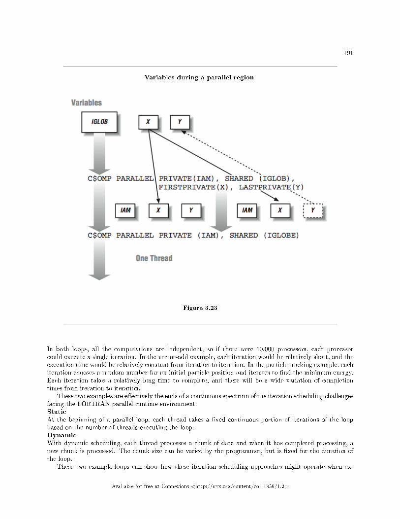
191
Variables during a parallel region
Figure 3.23
In both loops, all the computations are independent, so if there were 10,000 processors, each processorcould execute a single iteration. In the vector-add example, each iteration would be relatively short, and theexecution time would be relatively constant from iteration to iteration. In the particle tracking example, eachiteration chooses a random number for an initial particle position and iterates to �nd the minimum energy.Each iteration takes a relatively long time to complete, and there will be a wide variation of completiontimes from iteration to iteration.
These two examples are e�ectively the ends of a continuous spectrum of the iteration scheduling challengesfacing the FORTRAN parallel runtime environment:StaticAt the beginning of a parallel loop, each thread takes a �xed continuous portion of iterations of the loopbased on the number of threads executing the loop.DynamicWith dynamic scheduling, each thread processes a chunk of data and when it has completed processing, anew chunk is processed. The chunk size can be varied by the programmer, but is �xed for the duration ofthe loop.
These two example loops can show how these iteration scheduling approaches might operate when ex-
Available for free at Connexions <http://cnx.org/content/col11356/1.2>
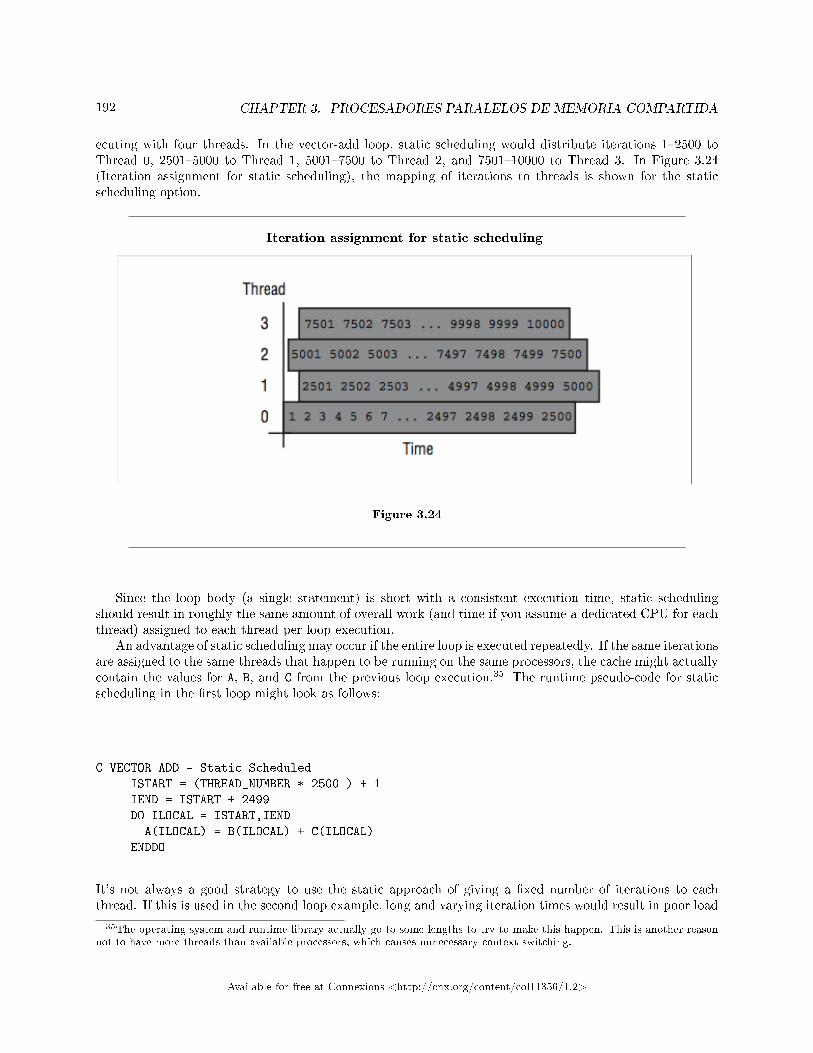
192 CHAPTER 3. PROCESADORES PARALELOS DE MEMORIA COMPARTIDA
ecuting with four threads. In the vector-add loop, static scheduling would distribute iterations 1�2500 toThread 0, 2501�5000 to Thread 1, 5001�7500 to Thread 2, and 7501�10000 to Thread 3. In Figure 3.24(Iteration assignment for static scheduling), the mapping of iterations to threads is shown for the staticscheduling option.
Iteration assignment for static scheduling
Figure 3.24
Since the loop body (a single statement) is short with a consistent execution time, static schedulingshould result in roughly the same amount of overall work (and time if you assume a dedicated CPU for eachthread) assigned to each thread per loop execution.
An advantage of static scheduling may occur if the entire loop is executed repeatedly. If the same iterationsare assigned to the same threads that happen to be running on the same processors, the cache might actuallycontain the values for A, B, and C from the previous loop execution.35 The runtime pseudo-code for staticscheduling in the �rst loop might look as follows:
C VECTOR ADD - Static Scheduled
ISTART = (THREAD_NUMBER * 2500 ) + 1
IEND = ISTART + 2499
DO ILOCAL = ISTART,IEND
A(ILOCAL) = B(ILOCAL) + C(ILOCAL)
ENDDO
It's not always a good strategy to use the static approach of giving a �xed number of iterations to eachthread. If this is used in the second loop example, long and varying iteration times would result in poor load
35The operating system and runtime library actually go to some lengths to try to make this happen. This is another reasonnot to have more threads than available processors, which causes unnecessary context switching.
Available for free at Connexions <http://cnx.org/content/col11356/1.2>
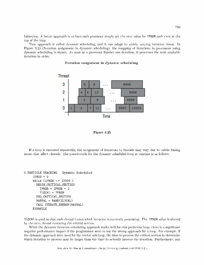
193
balancing. A better approach is to have each processor simply get the next value for IPROB each time at thetop of the loop.
That approach is called dynamic scheduling, and it can adapt to widely varying iteration times. InFigure 3.25 (Iteration assignment in dynamic scheduling), the mapping of iterations to processors usingdynamic scheduling is shown. As soon as a processor �nishes one iteration, it processes the next availableiteration in order.
Iteration assignment in dynamic scheduling
Figure 3.25
If a loop is executed repeatedly, the assignment of iterations to threads may vary due to subtle timingissues that a�ect threads. The pseudo-code for the dynamic scheduled loop at runtime is as follows:
C PARTICLE TRACKING - Dynamic Scheduled
IPROB = 0
WHILE (IPROB <= 10000 )
BEGIN_CRITICAL_SECTION
IPROB = IPROB + 1
ILOCAL = IPROB
END_CRITICAL_SECTION
RANVAL = RAND(ILOCAL)
CALL ITERATE_ENERGY(RANVAL)
ENDWHILE
ILOCAL is used so that each thread knows which iteration is currently processing. The IPROB value is alteredby the next thread executing the critical section.
While the dynamic iteration scheduling approach works well for this particular loop, there is a signi�cantnegative performance impact if the programmer were to use the wrong approach for a loop. For example, ifthe dynamic approach were used for the vector-add loop, the time to process the critical section to determinewhich iteration to process may be larger than the time to actually process the iteration. Furthermore, any
Available for free at Connexions <http://cnx.org/content/col11356/1.2>
194 CHAPTER 3. PROCESADORES PARALELOS DE MEMORIA COMPARTIDA
cache a�nity of the data would be e�ectively lost because of the virtually random assignment of iterationsto processors.
In between these two approaches are a wide variety of techniques that operate on a chunk of iterations.In some techniques the chunk size is �xed, and in others it varies during the execution of the loop. In thisapproach, a chunk of iterations are grabbed each time the critical section is executed. This reduces thescheduling overhead, but can have problems in producing a balanced execution time for each processor. Theruntime is modi�ed as follows to perform the particle tracking loop example using a chunk size of 100:
IPROB = 1
CHUNKSIZE = 100
WHILE (IPROB <= 10000 )
BEGIN_CRITICAL_SECTION
ISTART = IPROB
IPROB = IPROB + CHUNKSIZE
END_CRITICAL_SECTION
DO ILOCAL = ISTART,ISTART+CHUNKSIZE-1
RANVAL = RAND(ILOCAL)
CALL ITERATE_ENERGY(RANVAL)
ENDDO
ENDWHILE
The choice of chunk size is a compromise between overhead and termination imbalance. Typically theprogrammer must get involved through directives in order to control chunk size.
Part of the challenge of iteration distribution is to balance the cost (or existence) of the critical sectionagainst the amount of work done per invocation of the critical section. In the ideal world, the critical sectionwould be free, and all scheduling would be done dynamically. Parallel/vector supercomputers with hardwareassistance for load balancing can nearly achieve the ideal using dynamic approaches with relatively smallchunk size.
Because the choice of loop iteration approach is so important, the compiler relies on directives from theprogrammer to specify which approach to use. The following example shows how we can request the properiteration scheduling for our loops:
C VECTOR ADD
C$OMP PARALLEL DO PRIVATE(IPROB) SHARED(A,B,C) SCHEDULE(STATIC)
DO IPROB=1,10000
A(IPROB) = B(IPROB) + C(IPROB)
ENDDO
C$OMP END PARALLEL DO
C PARTICLE TRACKING
C$OMP PARALLEL DO PRIVATE(IPROB,RANVAL) SCHEDULE(DYNAMIC)
DO IPROB=1,10000
RANVAL = RAND(IPROB)
CALL ITERATE_ENERGY(RANVAL)
ENDDO
C$OMP END PARALLEL DO
Available for free at Connexions <http://cnx.org/content/col11356/1.2>
195
3.3.4 Closing Notes36
Using data �ow analysis and other techniques, modern compilers can peer through the clutter that weprogrammers innocently put into our code and see the patterns of the actual computations. In the �eld ofhigh performance computing, having great parallel hardware and a lousy automatic parallelizing compilergenerally results in no sales. Too many of the benchmark rules allow only a few compiler options to be set.
Physicists and chemists are interested in physics and chemistry, not computer science. If it takes 1 hour toexecute a chemistry code without modi�cations and after six weeks of modi�cations the same code executesin 20 minutes, which is better? Well from a chemist's point of view, one took an hour, and the other took1008 hours and 20 minutes, so the answer is obvious.37 Although if the program were going to be executedthousands of times, the tuning might be a win for the programmer. The answer is even more obvious if itagain takes six weeks to tune the program every time you make a modi�cation to the program.
In some ways, assertions have become less popular than directives. This is due to two factors: (1)compilers are getting better at detecting parallelism even if they have to rewrite some code to do so, and(2) there are two kinds of programmers: those who know exactly how to parallelize their codes and thosewho turn on the �safe� auto-parallelize �ags on their codes. Assertions fall in the middle ground, somewherebetween where the programmer does not want to control all the details but kind of feels that the loop canbe parallelized.
You can get online documentation of the OpenMP syntax used in these examples at www.openmp.org38
.
3.3.5 Exercises39
Exercise 3.3.5.1Take a static, highly parallel program with a relative large inner loop. Compile the application forparallel execution. Execute the application increasing the threads. Examine the behavior when thenumber of threads exceed the available processors. See if di�erent iteration scheduling approachesmake a di�erence.
Exercise 3.3.5.2Take the following loop and execute with several di�erent iteration scheduling choices. For chunk-based scheduling, use a large chunk size, perhaps 100,000. See if any approach performs better thanstatic scheduling:
DO I=1,4000000
A(I) = B(I) * 2.34
ENDDO
Exercise 3.3.5.3Execute the following loop for a range of values for N from 1 to 16 million:
DO I=1,N
36This content is available online at <http://cnx.org/content/m32820/1.3/>.37On the other hand, if the person is a computer scientist, improving the performance might result in anything from a poster
session at a conference to a journal article! This makes for lots of intra-departmental masters degree projects.38http://cnx.org/content/m32820/latest/www.openmp.org39This content is available online at <http://cnx.org/content/m32819/1.3/>.
Available for free at Connexions <http://cnx.org/content/col11356/1.2>
196 CHAPTER 3. PROCESADORES PARALELOS DE MEMORIA COMPARTIDA
A(I) = B(I) * 2.34
ENDDO
Run the loop in a single processor. Then force the loop to run in parallel. At what point do youget better performance on multiple processors? Do the number of threads a�ect your observations?
Exercise 3.3.5.4Use an explicit parallelization directive to execute the following loop in parallel with a chunk sizeof 1:
J = 0
C$OMP PARALLEL DO PRIVATE(I) SHARED(J) SCHEDULE(DYNAMIC)
DO I=1,1000000
J = J + 1
ENDDO
PRINT *, J
C$OMP END PARALLEL DO
Execute the loop with a varying number of threads, including one. Also compile and execute thecode in serial. Compare the output and execution times. What do the results tell you about cachecoherency? About the cost of moving data from one cache to another, and about critical sectioncosts?
Available for free at Connexions <http://cnx.org/content/col11356/1.2>
Chapter 4
Procesamiento Paralelo Escalable
4.1 Soporte del Lenguaje para Mejorar el Rendimiento
4.1.1 Soporte del Lenguaje para Mejorar el Rendimiento - Introducción1
Este capítulo discute los lenguajes de programación que se usan en los sistemas de procesamiento paralelomás grandes. Usualmente, cuando se tope con la necesidad de portar y a�nar su código para una nuevaarquitectura escalable, tendrá que sentarse durante algún tiempo a replantear su aplicación. A veces requeriráde hacer cambios fundamentales a su algoritmo antes de que pueda comenzar a usar la nueva arquitectura. Nose sorprenda si requiere reescribir todo o parte de la aplicación en uno de estos lenguajes. Las modi�cacionessobre un sistema bien pueden no reportar bene�cios de rendimiento sobre otro sistema distinto. Pero si laaplicación es lo su�cientemente importante, no importará el esfuerzo con tal de mejorar el rendimiento.
En este capítulo cubriremos:
• FORTRAN 90• HPF: High Performance FORTRAN
Estos lenguajes fueron diseñados para usarse en sistemas de cómputo de alto rendimiento. Crearemos paso apaso un pequeño programa en cada uno de ellos, usando un sencillo cálculo de diferencias �nitas que modelaaproximadamente un �ujo calórico. Se trata de un problema clásico que contiene una gran cantidad deparalelismo, y que puede resolverse fácilmente en una gran variedad de arquitecturas paralelas.
Introduciremos y discutiremos el concepto de SPMD (Simple Program, Multiple Data, Programa ÚnicoMúltiples Datos), mediante el cual tratamos a las computadoras MIMD como si fueran SIMD. Escribiremosnuestras aplicaciones tal como si estuviéramos usando un gran sistema SIMD para resolver el problema. Peroen vez de usar realmente tal sistema SIMD, la aplicación resultante se compilará para usarse en uno MIMD.La sincronización implícita de los sistemas SIMD será reemplazada en los sistemas MIMD por sincronizaciónexplícita a tiempo de ejecución.
4.1.2 Soporte del Lenguaje para Mejorar el Rendimiento - Problema de Datosen Paralelo: Flujo Calórico2
Un problema clásico que explota el procesamiento paralelo escalable, es la simulación de un �ujo calórico.La física tras este fenómeno descansa en una ecuación diferencial en derivadas parciales.
Comenzaremos con una placa de metal unidimensional (también conocida como una barra), y avanzare-mos hacia una placa bidimensional en los ejemplos posteriores. Al arranque, la barra se encuentra a cerogrados Celsius. Luego metemos uno de sus extremos en vapor a 100 grados, y el otro extremo en hielo a
1This content is available online at <http://cnx.org/content/m38316/1.1/>.2This content is available online at <http://cnx.org/content/m38317/1.1/>.
Available for free at Connexions <http://cnx.org/content/col11356/1.2>
197
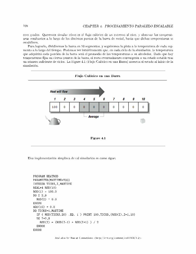
198 CHAPTER 4. PROCESAMIENTO PARALELO ESCALABLE
cero grados. Queremos simular cómo es el �ujo calórico de un extremo al otro, y observar las temperat-uras resultantes a lo largo de los distintos puntos de la barra de metal, hasta que dichas temperaturas seestabilicen.
Para lograrlo, dividiremos la barra en 10 segmentos, y seguiremos la pista a la temperatura de cada seg-mento a lo largo del tiempo. Podemos ver intuitivamente que, en cada ciclo de la simulación, la temperaturaque adquirirá cada porción de la barra será el promedio de las temperaturas a su alrededor. Dado que haytemperaturas �jas en ciertos puntos de la barra, el resto eventualmente convergerán a un estado estable trasun número su�ciente de ciclos. La Figure 4.1 (Flujo Calórico en una Barra) muestra el estado al inicio de lasimulación.
Flujo Calórico en una Barra
Figure 4.1
Una implementación simplista de tal simulación es como sigue:
PROGRAM HEATROD
PARAMETER(MAXTIME=200)
INTEGER TICKS,I,MAXTIME
REAL*4 ROD(10)
ROD(1) = 100.0
DO I=2,9
ROD(I) = 0.0
ENDDO
ROD(10) = 0.0
DO TICKS=1,MAXTIME
IF ( MOD(TICKS,20) .EQ. 1 ) PRINT 100,TICKS,(ROD(I),I=1,10)
DO I=2,9
ROD(I) = (ROD(I-1) + ROD(I+1) ) / 2
ENDDO
ENDDO
Available for free at Connexions <http://cnx.org/content/col11356/1.2>
199
100 FORMAT(I4,10F7.2)
END
La salida de este programa será la siguiente:
% f77 heatrod.f
heatrod.f:
MAIN heatrod:
% a.out
1 100.00 0.00 0.00 0.00 0.00 0.00 0.00 0.00 0.00 0.00
21 100.00 87.04 74.52 62.54 51.15 40.30 29.91 19.83 9.92 0.00
41 100.00 88.74 77.51 66.32 55.19 44.10 33.05 22.02 11.01 0.00
61 100.00 88.88 77.76 66.64 55.53 44.42 33.31 22.21 11.10 0.00
81 100.00 88.89 77.78 66.66 55.55 44.44 33.33 22.22 11.11 0.00
101 100.00 88.89 77.78 66.67 55.56 44.44 33.33 22.22 11.11 0.00
121 100.00 88.89 77.78 66.67 55.56 44.44 33.33 22.22 11.11 0.00
141 100.00 88.89 77.78 66.67 55.56 44.44 33.33 22.22 11.11 0.00
161 100.00 88.89 77.78 66.67 55.56 44.44 33.33 22.22 11.11 0.00
181 100.00 88.89 77.78 66.67 55.56 44.44 33.33 22.22 11.11 0.00
%
Claramente, para el ciclo de ejecución 101, la simulación converge con una precisión de dos decimales, con-forme los números han dejado de cambiar. Debe tratarse de una aproximación a un estado de temperaturasestables al centro de cada segmento de la barra.
Ahora bien, para este momento los lectores más astutos estarán diciéndose: "Ey, por si no te has dadocuenta, este ciclo tiene una dependencia de �ujo." Puede usted alegar que ello impedirá paralelizarlo siquieraun poquito. ½Es tan grave que ni siquiera puede usted deshacer el bucle para lograr algo de paralelismo anivel de instrucciones!
Una persona familiarizada con la teoría del �ujo calórico también pudiera señalar que el ciclo anteriorno implementa exactamente el modelo del �ujo calórico. El problema es que los valores en el lado derechode la asignación en el ciclo ROD, se supone que vienen del ciclo de ejecución anterior, y que el valor en ellado izquierdo es el que tendrá en el siguiente ciclo. Pero debido a la manera en que está escrito, el valorROD(I-1) viene desde el siguiente ciclo, como se muestra en la p. 199.
Este problema puede solucionarse usando una técnica conocida como rojo-negro, en la cual alternamosentre dos arreglos. La Figure 4.3 (Usando dos arreglos para eliminar una dependencia) muestra cómo opera(usando dos arreglos para eliminar una dependencia) la versión rojo-negro del cálculo. ½Mata dos pájarosde una sola pedrada! Ahora las matemáticas son precisamente correctas, y no hay recurrencia. Suena comouna situación realmente de ganar-ganar.
Available for free at Connexions <http://cnx.org/content/col11356/1.2>
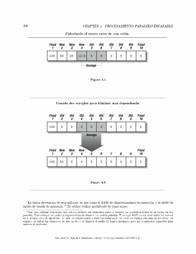
200 CHAPTER 4. PROCESAMIENTO PARALELO ESCALABLE
Calculando el nuevo valor de una celda.
Figure 4.2
Usando dos arreglos para eliminar una dependencia
Figure 4.3
La única desventaja de este enfoque, es que toma el doble de almacenamiento en memoria, y el doble deancho de banda de memoria. 3 El código código modi�cado es como sigue:
3Hay otro enfoque rojo-negro que calcula primero los elementos pares y después los elementos nones de la barra, en dospasadas. Este enfoque no presenta dependencias de datos entre ambas pasadas. El arreglo ROD nunca tiene todos los valoresen el mismo ciclo de ejecución. O bien los valores pares o bien los nones están un ciclo de tiempo adelante de los otros. Serequiere de saltar los elementos de dos en dos y se duplica el ancho de banda necesario, pero no la memoria requerida pararesolver el problema.
Available for free at Connexions <http://cnx.org/content/col11356/1.2>
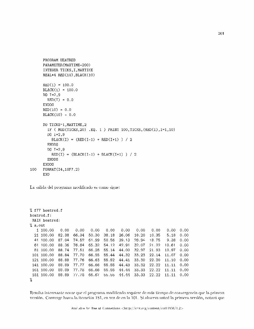
201
PROGRAM HEATRED
PARAMETER(MAXTIME=200)
INTEGER TICKS,I,MAXTIME
REAL*4 RED(10),BLACK(10)
RED(1) = 100.0
BLACK(1) = 100.0
DO I=2,9
RED(I) = 0.0
ENDDO
RED(10) = 0.0
BLACK(10) = 0.0
DO TICKS=1,MAXTIME,2
IF ( MOD(TICKS,20) .EQ. 1 ) PRINT 100,TICKS,(RED(I),I=1,10)
DO I=2,9
BLACK(I) = (RED(I-1) + RED(I+1) ) / 2
ENDDO
DO I=2,9
RED(I) = (BLACK(I-1) + BLACK(I+1) ) / 2
ENDDO
ENDDO
100 FORMAT(I4,10F7.2)
END
La salida del programa modi�cado es como sigue:
% f77 heatred.f
heatred.f:
MAIN heatred:
% a.out
1 100.00 0.00 0.00 0.00 0.00 0.00 0.00 0.00 0.00 0.00
21 100.00 82.38 66.34 50.30 38.18 26.06 18.20 10.35 5.18 0.00
41 100.00 87.04 74.52 61.99 50.56 39.13 28.94 18.75 9.38 0.00
61 100.00 88.36 76.84 65.32 54.12 42.91 32.07 21.22 10.61 0.00
81 100.00 88.74 77.51 66.28 55.14 44.00 32.97 21.93 10.97 0.00
101 100.00 88.84 77.70 66.55 55.44 44.32 33.23 22.14 11.07 0.00
121 100.00 88.88 77.76 66.63 55.52 44.41 33.30 22.20 11.10 0.00
141 100.00 88.89 77.77 66.66 55.55 44.43 33.32 22.22 11.11 0.00
161 100.00 88.89 77.78 66.66 55.55 44.44 33.33 22.22 11.11 0.00
181 100.00 88.89 77.78 66.67 55.55 44.44 33.33 22.22 11.11 0.00
%
Resulta interesante notar que el programa modi�cado requiere de más tiempo de convergencia que la primeraversión. Converge hasta la iteración 181, en vez de en la 101. Si observa usted la primera versión, notará que
Available for free at Connexions <http://cnx.org/content/col11356/1.2>
202 CHAPTER 4. PROCESAMIENTO PARALELO ESCALABLE
debido a la recurrencia, el calor terminaba �uyendo más rápido de izquierda a derecha, dado que el elementoizquierdo de cada promedio era el valor del siguiente ciclo de ejecución. Puede parecer ágil, pero está mal.4 Generalmente, en este problema, cualquier enfoque converge a los mismos valores eventuales dentro de loslímites de la representación de punto �otante.
El problema de �ujo calórico es extremadamente simple, y en su forma rojo-negro, resulta inherentementemuy paralelizable con interacciones muy simples de datos. Resulta un buen modelo para una amplia variedadde problemas en los cuales discretizamos espacios bidimensionales y tridimensionales, y realizamos algunasimulación sencilla en tales espacios.
Este problema usualmente puede escalarse creando una malla más �na. A menudo, el bene�cio de usarprocesadores escalables viene de permitir crear dichas mallas más �nas, y no de obtener soluciones en tiemposmás cortos. Por ejemplo, puede que usted sea capaz de realizar una simulación climática a nivel mundial,usando una malla con una separación de 200 millas, con un solo procesador en cuatro horas. Usando 100procesadores, puede que sea capaz de ejecutar la misma simulación usando un tamaño de malla de 20 millas,también en cuatro horas, pero con resultados mucho más precisos. O, utilizando 400 procesadores, puedehacer una simulación de malla aún más �na en una hora.
4.1.3 Soporte del Lenguaje para Mejorar el Rendimiento - Lenguajes Explícita-mente Paralelos5
Tal como hemos visto a lo largo de este libro, uno de los mayores retos de a�nación consiste en que elcompilador reconozca aquellos segmentos de código particulares que pueden paralelizarse. Esto resultaespecialmente cierto para códigos numéricos, donde el retorno de inversión es potencialmente mayor. Pienseen esto: si usted sabe que algo es paralelo, ¾por qué debiera haber alguna di�cultad en hacer que el compiladorlo reconozca? ¾Por qué no puede usted simplemente escribirlo, y hacer que el compilador diga "Sí, esto sehará en paralelo"?
El problema es que los lenguajes de programación más comúnmente usados no ofrecen ningún constructopara expresar cálculos en paralelo. Usted se ve forzado a expresarse en términos primitivos, como si fueraun cavernícola con grandes ideas, pero sin vocabulario para explicarlas. Esto es particularmente cierto enFORTRAN y en C, que no soportan la noción de cómputos en paralelo, lo cuál signi�ca que los programadoresdeben reducir los cálculos a pasos secuenciales. Suena incómodo, pero la mayoría de los programadores lohacen de forma tan natural que ni siquiera se percatan de cuán buenos son para ello.
Por ejemplo, digamos que queremos sumar dos vectores, A y B. ¾Cómo debemos hacerlo? Probablementeescribamos un pequeño ciclo sin siquiera detenernos un instante a pensarlo:
DO I=1,N
C(I) = A(I) + B(I)
END DO
Parece razonable, pero veamos qué pasa. ½Le hemos impuesto un orden a los cálculos! ¾No hubiera bastadocon decir "C es el resultado de A más B"? Ello permitiría al compilador sumar los vectores usando cua-lesquiera hardware a su disposición, usando el método que mejor le parezca. De eso se tratan los lenguajesparalelos, de proporcionar primitivas capaces de expresar cómputos paralelos.
4Existen otros enfoques algorítmicos para resolver las ecuaciones diferenciales en derivadas parciales, tales como el "métodorápido multipolo" que acelera la convergencia "legalmente". No asuma que el enfoque de fuerza bruta usado aquí es el únicométodo para resolver este problema en particular. Los programadores siempre deben buscar el mejor algoritmo disponible (seao no paralelo) antes de intentar escalar el algoritmo "equivocado". Para aquellos cuates que no son cientí�cos en computación,el tiempo para la solución es más importante que el incremento lineal de velocidad.
5This content is available online at <http://cnx.org/content/m38318/1.1/>.
Available for free at Connexions <http://cnx.org/content/col11356/1.2>
203
No se están proponiendo nuevos lenguajes paralelos tan rápidamente como se hizo a mediados de ladécada de 1980. Los desarrolladores se han dado cuenta que pueden crear un esquema maravilloso, perosi no es compatible con FORTRAN o C, le va a interesar a poca gente. La razón es simple: hay miles demillones de líneas de código C y FORTRAN, pero sólo unas pocas en Fizgibbet o como sea que le llameusted a su nuevo lenguaje paralelo. Por causa de la preminencia de C y FORTRAN, las actividades mássigni�cativas referentes a lenguajes paralelos que se desarrollan actualmente se enfocan a extender estoslenguajes, protegiendo así 20 o 30 años de inversión en programas ya escritos. 6 Resulta muy tentador paralos desarrolladores de un nuevo lenguaje probarlo mediante el problema de las ocho reinas y el juego dela vida, obtener buenos resultados, y luego declarar que está listo para su debut y esperar que hordas deprogramadores lo conviertan en su lenguaje de cabecera.
4.1.4 Soporte del Lenguaje para Mejorar el Rendimiento - FORTRAN 907
La versión previa del estandar de FORTRAN liberada por ANSI (el American National Standard Institute),FORTRAN 77 (X3.9-1978) se escribió para promover la portabilidad de los programas FORTRAN entreplataformas distintas. No se inventaron nuevos componentes del lenguaje, más bien se incorporaron buenascaracterísticas que ya estaban disponibles en compiladores en ambientes de producción. Al contrario queFORTRAN 77, el FORTRAN 90 (ANSI X3.198-1992) añade nuevas extensiones y características al lenguaje.Algunas de ellas sólo ponen al día a FORTRAN respecto a lenguajes como C (asignación dinámica dememoria, reglas de alcance) y C++ (interfaces de funciones con genericidad). Pero algunas de estas nuevascaracterísticas son únicas de FORTRAN (operaciones sobre arreglos). Es interesante notar que mientras sedesarrollaba la especi�cación de FORTRAN 90, las arquitecturas de cómputo de alto rendimiento dominanteseran los sistemas SIMD escalables como la Connection Machine, así como los sistemas de procesadoresvectoriales paralelos de compañías como Cray Research.
FORTRAN 90 hace un trabajo sorprendentemente bueno en cubrir las necesidades de estas arquitecturastan diferentes. Sus características también se adaptan razonablemente bien a los nuevos multiprocesadorescon memoria compartida uniforme. Sin embargo, como veremos después, FORTRAN 90 por sí solo todavíano es su�ciente para cumplir las necesidades de los sistemas distribuidos escalables con acceso a memoria nouniforme, que se están volviendo dominantes en la computación de extremo superior.
Las extensiones de FORTRAN 90 a FORTRAN 77 incluyen:
• Constructos para arreglos• Asignación dinámica de memoria y variables automáticas• Apuntadores• Nuevos tipos de datos, estructuras• Nuevas funciones intrínsecas, incluyendo muchas que operan sobre vectores y matrices• Nuevas estructuras de control, tales como la sentencia WHERE• Interfaces de procedimientos mejoradas
4.1.4.1 Constructos para Arreglos en FORTRAN 90
Con los constructos para arreglos de FORTRAN 90, puede usted especi�car arreglos completos o seccionesde los mismos como participantes en operaciones unarias y binarias. Tales constructos son una característicaclave para "deserializar" las aplicaciones, de forma que puedan adaptarse mejor a computadoras vectorialeso procesadores paralelos. Por ejemplo, digamos que desea usted sumar dos vectores A y B. En FORTRAN90, puede expresarlo como una simple operación de suma, en vez de usando el bucle tradicional. Esto es,puede usted escribir:
6Uno de los esfuerzos más signi�cativos en el campo de los lenguajes completamente nuevos es SISAL (Streams and Iterationin a Single Assignment Language). Es un lenguaje de �ujo de datos que se puede integrar fácilmente en módulos de FORTRANy C. Los aspectos más interesantes de SISAL son la cantidad de código que se ha portado a SISAL, y el hecho de que losdesarrolladores de SISAL generalmente comparan su rendimiento con el de aplicaciones iguales en FORTRAN y C.
7This content is available online at <http://cnx.org/content/m38320/1.1/>.
Available for free at Connexions <http://cnx.org/content/col11356/1.2>
204 CHAPTER 4. PROCESAMIENTO PARALELO ESCALABLE
A = A + B
en vez del tradicional bucle en FORTRAN 77:
DO I=1,N
A(I) = A(I) + B(I)
ENDDO
Puede que el código generado por el compilador en su estación de trabajo no se vea muy diferente, pero enalgunas máquinas de arquitectura paralela o en algunas estaciones de trabajo a la vuelta de la esquina, ladiferencia es signi�cativa. La versión FORTRAN 90 declara explícitamente que los cálculos pueden realizarseen cualquier orden, incluyendo todos en paralelo simultáneamente.
Un efecto importante de ello es que si la versión de FORTRAN 90 experimenta una falla de punto �otantesumando el elemento 17, y revisa usted la memoria en un depurador, encontrará que el elemento 27 ya fuecalculado y tiene un valor perfectamente válido.
Y no está usted limitado tan sólo a arreglos unidimensionales. Por ejemplo, la suma a nivel de elementosde dos arreglos bidimensionales puede realizarse así:8
A = A + B
en vez de:
DO J=1,M
DO I=1,N
A(I,J) = A(I,J) + B(I,J)
END DO
END DO
Naturalmente, si desea combinar dos arreglos en una operación, sus tamaños tienen que ser compatibles.Sumar un vector de siete elementos a uno de ocho no tiene sentido. Tampoco lo tiene multiplicar un arreglode 2*4 a uno de 3*4.. Cuando los dos arreglos tienen tamaños compatibles, relativos a la operación a quequiere usted someterlos, decimos que tienen concordancia de tamaños, como en el siguiente código:
8Sólo en caso de que esté usted sorprendido, A*B regresa el producto de los miembros del arreglo a nivel de elementos, noel producto de dos matrices. Tal operación la cubre FORTRAN 90 mediante una función intrínseca.
Available for free at Connexions <http://cnx.org/content/col11356/1.2>
205
DOUBLE PRECISION A(8), B(8)
...
A = A + B
Siempre se considera que los escalares tienen concordancia de tamaños con los arreglos (y con otros escalares).En una operación binaria con un arreglo, un escalar se trata como un arreglo del mismo tamaño, con el únicoelemento duplicado en el resto de las posiciones.
Aun así, existen limitaciones. Cuando haga referencia a un arreglo particular, por ejemplo A, estáhaciendo referencia a todo él, del primer al último elemento. Seguro puede usted imaginar casos donde leinterese especi�car un subconjunto de un arreglo. Puede tratarse de un grupo de elementos consecutivos oalgo como "cada octavo elemento" (i.e. un recorrido de salto no unitario a través del arreglo). A tales partesde los arreglos, posiblemente no contiguas, se les denomina secciones del arreglo.
Para especi�car secciones de arreglos en FORTRAN 90, se reemplazan los índices tradicionales contripletas de la forma a:b:c, que signi�can "los elementos desde a hasta b, tomados con un incremento de c."Pueden omitirse partes de la tripleta, siempre y cuando el signi�cado permanezca claro. Por ejemplo, a:bsigni�ca "los elementos desde a hasta b;" a: signi�ca "los elementos desde a hasta el extremo superior delarreglo con un incremento de 1." Recuerdo que una tripleta reemplaza a un único índice, así que un arreglon-dimensional puede tener n tripletas.
Puede usted usar tripletas en expresiones, nuevamente asegurándose de que las partes de las expresionesestén en concordancia. Considere estos ejemplos:
REAL X(10,10), Y(100)
...
X(10,1:10) = Y(91:100)
X(10,:) = Y(91:100)
La primera sentencia asigna los últimos 10 elementos de Y al décimo renglón de X. La segunda sentenciaexpresa lo mismo de modo ligeramente diferente. El " : " solitario le indica al compilador que está implícitoel rango completo (del 1 al 10).
4.1.4.2 Intrínsecos en FORTRAN 90
FORTRAN 90 extiende la funcionalidad de los intrínsecos de FORTRAN 77, y además agrega muchosnuevos, incluyendo algunas subrutinas intrínsecas. La mayoría pueden ser valoradas mediante arreglos:pueden regresar secciones de arreglos o escalares, dependiendo de cómo fueron invocadas. Por ejemplo, heaquí un nuevo uso del intrínseco SIN valorado mediante arreglos:
REAL A(100,10,2)
...
A = SIN(A)
Cada elemento del arreglo A es reemplazado por su seno. Los intrínsecos de FORTRAN 90 también trabajancon secciones de arreglos, con tal de que la variable que reciba los resultados esté en concordancia de tamañocon la que se pasó:
Available for free at Connexions <http://cnx.org/content/col11356/1.2>
206 CHAPTER 4. PROCESAMIENTO PARALELO ESCALABLE
REAL A(100,10,2)
REAL B(10,10,100)
...
B(:,:,1) = COS(A(1:100:10,:,1))
También se han extendido otros intrínsecos tales como SQRT, LOG, etc. Entre los nuevos intrínsecos seencuentran:
Reducciones: FORTRAN 90 tiene reducciones de vectores tales como MAXVAL, MINVAL y SUM. Para arreglosde orden superior (cualquier cosa mayor que un vector) tales funciones pueden realizar una reduccióna lo largo de una dimensión en particular. Adicionalmente, existe una función DOT_PRODUCT (productopunto) para los vectores.
Manipulación de matrices: Los intrínsecos MATMUL y TRANSPOSE pueden manipular matrices completas.Construir o redimensionar arreglos: RESHAPE le permite crear un nuevo arreglo a partir de los elementos
de uno antiguo con diferente tamaño. SPREAD replica un arreglo a lo largo de una nueva dimensión.MERGE copia porciones de un arreglo en otro, bajo el control de una máscara. CSHIFT permite desplazarun arreglo en una o más dimensiones.
Funciones de consulta: SHAPE, SIZE, LBOUND, y UBOUND le permiten averiguar cómo está construido unarreglo.
Pruebas en paralelo: Dos intrínsecos nuevos de reducción, ANY y ALL, sirven para probar en paralelo varioselementos de un arreglo.
4.1.4.3 Nuevas Características de Control
FORTRAN 90 incluye algunas nuevas características de control, entre ellas una primitiva de asignacióncondicional llamada WHERE, que pone las asignaciones de un arreglo con concordancia de tamaños bajo elcontrol de una máscara, tal como en el ejemplo siguiente. He aquí un ejemplo de la primitiva WHERE:
REAL A(2,2), B(2,2), C(2,2)
DATA B/1,2,3,4/, C/1,1,5,5/
...
WHERE (B .EQ. C)
A = 1.0
C = B + 1.0
ELSEWHERE
A = -1.0
ENDWHERE
En aquellos casos donde la expresión lógica es TRUE, A obtiene 1.0 y C obtiene B+1.0. En la claúsulaELSEWHERE, A obtiene -1.0. El resultado de la operación anterior serán los arreglos A y C con los elementos:
A = 1.0 -1.0 C = 2.0 5.0
Available for free at Connexions <http://cnx.org/content/col11356/1.2>
207
-1.0 -1.0 1.0 5.0
Nuevamente, no hay ningún orden implícito en estas asignaciones condicionales, lo cual signi�ca que puedenrealizarse en paralelo. La ausencia de orden implícito es crítica para permitir a los sistemas de cómputoSIMD y a los ambientes SPMD tener �exibilidad en la ejecución de tales cálculos.
4.1.4.4 Arreglos Automáticos y Asignables
Cada programa requiere variables temporales o espacio de trabajo. En el pasado, los programadores deFORTRAN a menudo administraban su propio espacio libre, declarando un arreglo lo su�cientemente grandepara manejar cualquier requerimiento temporal. Esta práctica se traga la memoria (aunque la memoriavirtual, por lo general), e incluso puede tener efectos indeseados en el rendimiento. Con la habilidad deasignar la memoria dinámicamente, los programadores pueden esperar más tiempo para decidir cuántoespacio vacío deben obtener. FORTRAN 90 soporta la asignación dinámica de memoria mediante dosnuevas características del lenguaje: arreglos automáticos y arreglos asignables.
Tal como sucede con las variables locales de un programa en C, los arreglos automáticos de FORTRAN90 sólo tienen asignado espacio de almacenamiento durante la vida de la subrutina o función que los contiene.Esto es diferente del almacenamiento local de arreglos tradicional de FORTRAN, donde algo de espacio seapartaba a tiempo de compilación o enlace. El tamaño y forma de los arreglos automáticos puede esculpirsemediante ua combinación de constantes y argumentos. Por ejemplo, he aquí una declaración de un arregloautomático, B, usando la nueva especi�cación de sintaxis de FORTRAN 90:
SUBROUTINE RELAX(N,A)
INTEGER N
REAL, DIMENSION (N) :: A, B
Se declararon dos arreglos: A, el argumento de prueba, y B, un arreglo automático de tamaño explícito.Cuando se regresa de la subrutina, B deja de existir. Observe que el tamaño de B se toma de uno de losargumentos, N.
Los arreglos asignables le dan a usted la �exibilidad de elegir el tamaño de un arreglo después de examinarotras variables en el programa. Por ejemplo, puede que desee determinar la cantidad de datos de entradaantes de asignar los arreglos. Este pequeño programa pregunta al usuario el tamaño de la matriz antes deasignarle espacio de almacenamiento:
INTEGER M,N
REAL, ALLOCATABLE, DIMENSION (:,:) :: X
...
WRITE (*,*) 'INTRODUZCA LAS DIMENSIONES DE X'
READ (*,*) M,N
ALLOCATE (X(M,N))
...
hacer algo con X
...
DEALLOCATE (X)
...
Available for free at Connexions <http://cnx.org/content/col11356/1.2>
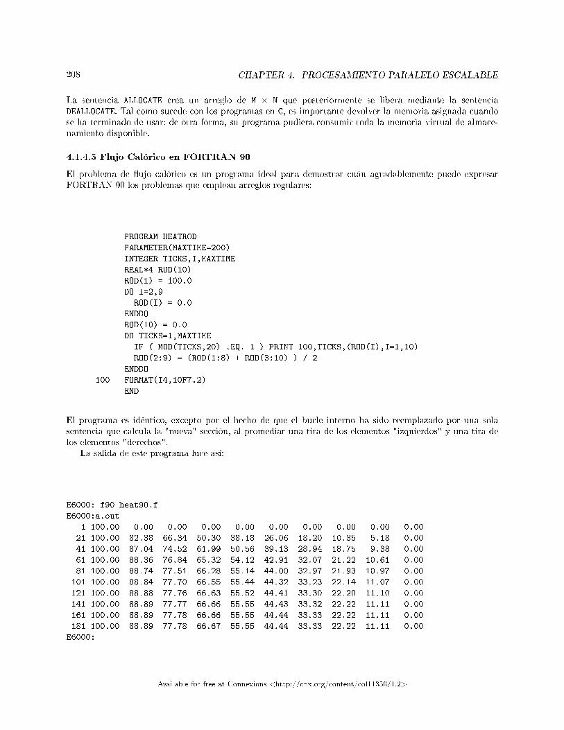
208 CHAPTER 4. PROCESAMIENTO PARALELO ESCALABLE
La sentencia ALLOCATE crea un arreglo de M × N que posteriormente se libera mediante la sentenciaDEALLOCATE. Tal como sucede con los programas en C, es importante devolver la memoria asignada cuandose ha terminado de usar; de otra forma, su programa pudiera consumir toda la memoria virtual de almace-namiento disponible.
4.1.4.5 Flujo Calórico en FORTRAN 90
El problema de �ujo calórico es un programa ideal para demostrar cuán agradablemente puede expresarFORTRAN 90 los problemas que emplean arreglos regulares:
PROGRAM HEATROD
PARAMETER(MAXTIME=200)
INTEGER TICKS,I,MAXTIME
REAL*4 ROD(10)
ROD(1) = 100.0
DO I=2,9
ROD(I) = 0.0
ENDDO
ROD(10) = 0.0
DO TICKS=1,MAXTIME
IF ( MOD(TICKS,20) .EQ. 1 ) PRINT 100,TICKS,(ROD(I),I=1,10)
ROD(2:9) = (ROD(1:8) + ROD(3:10) ) / 2
ENDDO
100 FORMAT(I4,10F7.2)
END
El programa es idéntico, excepto por el hecho de que el bucle interno ha sido reemplazado por una solasentencia que calcula la "nueva" sección, al promediar una tira de los elementos "izquierdos" y una tira delos elementos "derechos".
La salida de este programa luce así:
E6000: f90 heat90.f
E6000:a.out
1 100.00 0.00 0.00 0.00 0.00 0.00 0.00 0.00 0.00 0.00
21 100.00 82.38 66.34 50.30 38.18 26.06 18.20 10.35 5.18 0.00
41 100.00 87.04 74.52 61.99 50.56 39.13 28.94 18.75 9.38 0.00
61 100.00 88.36 76.84 65.32 54.12 42.91 32.07 21.22 10.61 0.00
81 100.00 88.74 77.51 66.28 55.14 44.00 32.97 21.93 10.97 0.00
101 100.00 88.84 77.70 66.55 55.44 44.32 33.23 22.14 11.07 0.00
121 100.00 88.88 77.76 66.63 55.52 44.41 33.30 22.20 11.10 0.00
141 100.00 88.89 77.77 66.66 55.55 44.43 33.32 22.22 11.11 0.00
161 100.00 88.89 77.78 66.66 55.55 44.44 33.33 22.22 11.11 0.00
181 100.00 88.89 77.78 66.67 55.55 44.44 33.33 22.22 11.11 0.00
E6000:
Available for free at Connexions <http://cnx.org/content/col11356/1.2>
209
Si lo observa detenidamente, verá que la salida es la misma que la de la implementación rojo-negro. Ello sedebe a que en FORTRAN 90:
ROD(2:9) = (ROD(1:8) + ROD(3:10) ) / 2
es una única sentencia de asignación. Como se muestra en Figure 4.4 (Alineación de datos y cálculos), laparte derecha se evalúa completamente antes de que la sección del arreglo resultante se le asigne a ROD(2:9).A primera vista puede parecer poco natural, pero considere la siguiente sentencia:
I = I + 1
Sabemos que si I comienza en 5, esta sentencia incrementará su valor a 6. Ello sucede porque el lado derecho(5+1) se evalúa antes de ejecutar la asignación del 6 a I. En FORTRAN 90, una variable puede ser unarreglo completo. Así que ésta is una operación rojo-negro. ½Hay un ROD "antiguo" en la parte derecha, yun ROD "nuevo" en la parte izquierda!
Para realmente "pensar" al estilo FORTRAN 90, es bueno suponer que está usted usando un sistemaSIMD con millones de pequeñas CPUs. Primero alineamos cuidadosamente los datos, deslizándolos alrededor,y entonces... ½zas! en una sola instrucción, sumamos todos los valores alineados en un solo instante. Figure 4.4(Alineación de datos y cálculos) muestra grá�camente este acto de "alinear" los valores y luego sumarlos.El grafo de �ujo de datos es extremadamente simple. Los dos renglones superiores son de sólo lectura, y losdatos �uyen de arriba hacia abajo. Usar el espacio temporal elimina la dependencia aparente. Este enfoquede "pensar SIMD" es una de dos formas posibles de obligarnos a enfocar nuestro pensamiento en los datos,en vez de en el control. Puede que la SIMD no sea una buena arquitectura para nuestro problema, pero sies capaz de expresarlo de forma tal que pueda trabajarse en SIMD, un buen ambiente SPMD puede tomarventaja del paralelismo a nivel de datos que usted ha identi�cado.
El ejemplo siguiente pone de mani�esto uno de los retos que aparecen al producir una implementacióne�ciente de FORTRAN 90. Si estos arreglos contienen 10 millones de elementos, y el compilador usa unenfoque simple, necesitará 30 millones de elementos para los valores "izquierdos" viejos, los valores "derechos"viejos y para los nuevos. Se requiere optimizar el �ujo de datos sólo para determinar para determinar cuántosdatos extras deben mantenerse para obtener los resultados apropiados. Si el compilador es inteligente, lamemoria extra puede ser muy poca:
Available for free at Connexions <http://cnx.org/content/col11356/1.2>
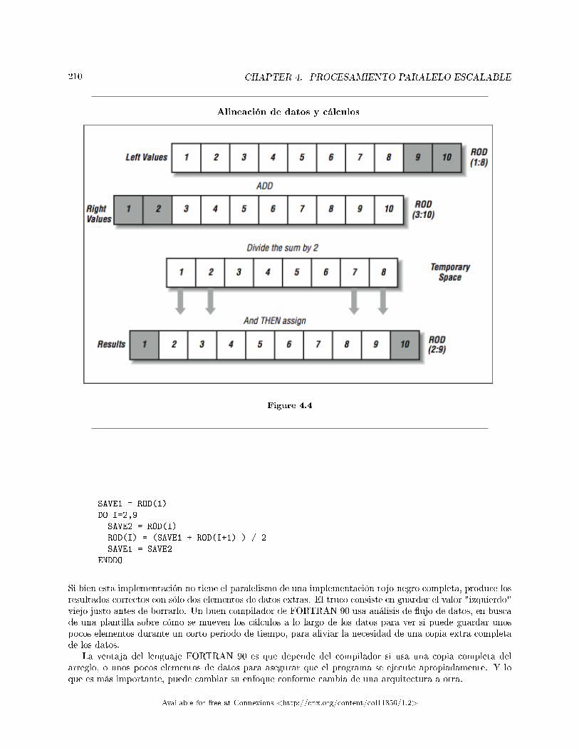
210 CHAPTER 4. PROCESAMIENTO PARALELO ESCALABLE
Alineación de datos y cálculos
Figure 4.4
SAVE1 = ROD(1)
DO I=2,9
SAVE2 = ROD(I)
ROD(I) = (SAVE1 + ROD(I+1) ) / 2
SAVE1 = SAVE2
ENDDO
Si bien esta implementación no tiene el paralelismo de una implementación rojo-negro completa, produce losresultados correctos con sólo dos elementos de datos extras. El truco consiste en guardar el valor "izquierdo"viejo justo antes de borrarlo. Un buen compilador de FORTRAN 90 usa análisis de �ujo de datos, en buscade una plantilla sobre cómo se mueven los cálculos a lo largo de los datos para ver si puede guardar unospocos elementos durante un corto periodo de tiempo, para aliviar la necesidad de una copia extra completade los datos.
La ventaja del lenguaje FORTRAN 90 es que depende del compilador si usa una copia completa delarreglo, o unos pocos elementos de datos para asegurar que el programa se ejecute apropiadamente. Y loque es más importante, puede cambiar su enfoque conforme cambia de una arquitectura a otra.
Available for free at Connexions <http://cnx.org/content/col11356/1.2>
211
4.1.4.6 FORTRAN 90 Versus FORTRAN 77
Es interesante señalar que FORTRAN 90 nunca fue completamente adoptado por la comunidad de cómputode alto rendimiento. Existen algunas razones para ello:
• Existía la preocupación de que el uso de apuntadores y estructuras de datos dinámicas arruinase elrendimiento, y se perdieran las ventajas de optimización de FORTRAN sobre C. Algunos dijeron queFORTRAN 90 estaba tratando de ser un mejor C que C. Otros decían, "¾quién quiere parecerse mása un lenguaje más lento?" Sea cual fuere la razón, hubo algo de controversia cuando se implementóFORTRAN 90, que derivó en algo de reluctancia de los programadores para adoptarlo. Algunosvendedores decían "Puede usted usar FORTRAN 90, pero FORTRAN 77 siempre será más rápido."
• Y como los vendedores a menudo implementaron diferentes subconjuntos de FORTRAN 90, el códigono fue tan transportable como el de FORTRAN 77. Por tal motivo, los usuarios que requerían máximatransportabilidad continuaron con FORTRAN 77.
• A veces los vendedores compraban sus compiladores que cumplían completamente con FORTRAN 90a terceros, quienes cobraban altas tarifas de licenciamiento. Así, podía usted obtener un FORTRAN77 gratuito (y más rápido, de acuerdo con el vendedor) o pagar por el compilador de FORTRAN 90más lento (guiño, guiño).
• Por tales factores, el número de aplicaciones serias desarrolladas en FORTRAN 90 fue pequeño. Así quelos bancos de pruebas usados para comprar nuevos sistemas estaban desarrollados casi exclusivamenteen FORTRAN 77. Ello motivó a los vendedores a mejorar sus compiladores de FORTRAN 77 en vezde sus compiladores de FORTRAN 90.
• Conforme los compiladores de FORTRAN 77 se hacían más so�sticados, usando análisis de �ujo dedatos, fue relativamente fácil escribir código "paralelo" transportable en FORTRAN 77, usando lastécnicas que hemos discutido en este libro.
• Uno de los mayores bene�cios potenciales de FORTRAN 90 era la transportabilidad entre SIMD ylas supercomputadoras paralelas/vectoriales. Conforme ambas arquitecturas fueron reemplazadas conmultiprocesadores con memoria uniforme compartida, FORTRAN 77 se convirtió en el lenguaje queofrecía la máxima transportabilidad entre las computadoras usadas típicamente por los programadoresde cómputo de alto rendimiento.
• Los compiladores de FORTRAN 77 soportaban directivas que permitían a los programadores a�nar�namente el rendimiento de sus aplicaciones, al tomar completo control del paralelismo. Ciertos dialec-tos de FORTRAN 77 esencialmente se convirtieron en un "lenguaje ensamblador" para programaciónparalela. Incluso las versiones altamente a�nadas de tales códigos eran relativamente transportablesentre multiprocesadores de memoria compartida uniforme de diferentes vendedores.
Así que los eventos conspiraron contra FORTRAN 90 en el corto plazo. Sin embargo, FORTRAN 77 noestá bien adaptado a los sistemas de memoria distribuida porque no se presta bien para las directivas dedisposición de datos. Conforme requerimos particionar y distribuir los datos cuidadosamente sobre esosnuevos sistemas, debemos dar al compilador gran cantidad de �exibilidad. FORTRAN 90 es el lenguajemejor adaptado para tal propósito.
4.1.4.7 Resumen de FORTRAN 90
Bueno, este es una visita apresurada a FORTRAN 90. Probablemente no le hayamos hecho justicia allenguaje cubriéndolo tan brevemente, pero queremos que usted se lleve una probada del mismo. Hay muchascaracterísticas que no hemos discutido. Si quiere aprender más, le recomendamos FORTRAN 90 Explained,de Michael Metcalf y John Reid (Oxford University Press).
FORTRAN 90 no es su�ciente por sí mismo para que obtengamos rendimiento escalable en sistema dememoria distribuida. Es más, ningún compilador es todavía capaz de realizar su�ciente análisis de datospara decidir dónde almacenar los datos y cuándo recuperarlos de la memoria. Así, por ahora, nosotros comoprogramadores debemos preocuparnos por la disposición de los datos. Debemos descomponer el problemaen fragmentos paralelos que puedan procesarse individualmente. Tenemos varias opciones. Podemos usar
Available for free at Connexions <http://cnx.org/content/col11356/1.2>

212 CHAPTER 4. PROCESAMIENTO PARALELO ESCALABLE
High Performance FORTRAN y delegar algunos detalles al compilador, o podemos usar paso de mensajesexplícito y ocuparnos nosotros mismos de todos los detalles del paralelismo.
4.1.5 Soporte del Lenguaje para Mejorar el Rendimiento - Descomposición delProblema9
Existen tres enfoques principales sobre cómo dividir o descomponer un trabajo, de modo que pueda dis-tribuirse entre múltiples CPUs:
Descomposición de los cálculos: Ya hemos discutido esta técnica. Cuando la descomposición se hacebasándose en los cálculos, llegamos a algún mecanismo para dividir equitativamente los cómputos (talescomo las iteraciones o un bucle) entre nuestros procesadores. Generalmente se ignora la ubicación delos datos, y las preocupaciones principales son la duración de cada iteración y la uniformidad. Estaes la técnica predilecta para los sistemas de memoria uniformemente compartida, porque cualquierprocesador puede acceder a los datos de modo igualitario.
Decomposición de los datos: Cuando el acceso a la memoria no es uniforme, la tendencia es enfocarseen la distribución de los datos en vez de los cómputos. Se asume que la recuperación de los datos"remotos" es costosa y por tanto debe minimizarse. Los datos se distribuyen entre las memorias. Elprocesador que contiene el dato realiza los cálculos sobre dicho dato tras recuperar cualquier otro datonecesario para realizarlos.
Decomposición de las tareas: Cuando las operaciones que deben realizarse son muy independientes entresí, y toman algún tiempo, puede llevarse a cabo una descomposición de tareas. En este enfoqueun proceso o hilo de ejecución maestro mantiene una cola de las unidades de trabajo. Cuando unprocesador dispone de recursos, recupera la siguiente "tarea" de la cola y comienza a procesarla. Setrata de un enfoque muy atractivo para cálculos embarazosamente paralelos.10
En cierto sentido, el resto del capítulo está dedicado primordialmente a la descomposición de datos. En unsistema de memoria distribuida, el costo de comunicación usualmente es el factor de rendimiento dominante.Si su problema es tan violentamente paralelo que puede distribuirse entre tareas, prácticamente cualquiertécnica funcionará. Los problemas con datos paralelos ocurren en muchas disciplinas. Pueden variar desdeaquellos que son extremadamente paralelos, a aquellos otros que sólo lo son un poco. Por ejemplo, loscálculos fractales son extremadamente paralelos; cada punto se deriva independientemente del resto. Essencillo dividir los cálculos fractales entre los procesadores. Y dado que los cálculos son independientes, losprocesadores no requieren coordinarse o compartir datos.
Nuestro problema de �ujo calórico, cuando se expresa en su forma rojo-negro (o FORTRAN 90) esextremadamente paralelo, pero requiere de cierto grado de compartición de datos. Un modelo gravitatorioo una galaxia es otra clase de programa paralelo. Cada punto ejerce una in�uencia sobre cualesquiera otro.Así, y al contrario que los cálculos fractales, los procesadores deben compartir datos.
Sea cual sea el caso, usted quiere acomodar los cálculos de forma que los procesadores puedan decirselos unos a los otros, "empieza a partir de aquí y trabaja en esto, mientras que yo trabajo en esto otro, y loreuniremos nuevamente cuando hayamos terminado."
Aun los problemas que ofrecen menos independencia entre regiones son todavía muy buenos candidatospara la descomposición del dominio. Los problemas de diferencias �nitas, la simulación de la interacción entrepartículas próximas, y las columnas de matrices pueden tratarse de forma similar. Si puede usted dividirel dominio igualmente entre los procesadores, cada uno realizará aproximadamente la misma cantidad detrabajo en su camino hacia la solución.
Otros sistemas físicos no son tan regulares, o involucran interacciones de rango aomplio. Los nodos deuna rejilla no estructurada pueden no estar acomodados en correspondencia directa con sus ubicaciones
9This content is available online at <http://cnx.org/content/m38329/1.1/>.10El esfuerzo distribuido para romper la clave RC5 fue coordinado de esta forma. Cada procesador recibió un bloque de
claves y comenzó a probar dichas claves. En algún punto, si los procesadores no eran lo su�cientemente rápidos o dejaban defuncionar, el sistema central reasignaba el bloque a otro procesador. Esto permite al sistema recuperarse de problemas en lascomputadoras individuales.
Available for free at Connexions <http://cnx.org/content/col11356/1.2>
213
físicas, por ejemplo. O tal vez el modelo involucre fuerzas de rango amplio, tales como la atracción entrepartículas. Estos problemas también pueden estructurarse para máquinas paralelas, aunque resulte algomás difícil. A veces se requiere de varias simpli�caciones, o de "agrupamiento" de efectos intermedios. Porejemplo, la in�uencia de un grupo de partículas distantes sobre otro puede tratarse como si se tratar departículas compuestas actuando a distancia. Con ello se ahorran las comunicaciones que se requieren quecada procesador haga para hablar con cada uno de los otros, acerca de cada detalle. En otros casos, laarquitectura paralela ofrece oportunidades de expresar un sistema físico en formas distintas e ingeniosas,que tienen sentido en el contexto de la máquina. Por ejemplo, puede asignarse cada partícula a su propioprocesador, de forma que puedan deslizarse unas sobre otras, agregando interacciones y actualizando un ciclode tiempo.
Dependiendo de la arquitectura de la computadora paralela y del problema, elegir entre dividir o replicar(porciones de) el dominio puede agregar una sobrecarga de trabajo o costos inaceptables para todo el proyecto.
En problemas grandes, el costo económico de la memoria principal puede dejar fuera de toda discusiónel mantener copias locales separadas del mismo dato. De hecho, a menudo es la necesidad de más memorialo que conduce a las personas hacia las máquinas paralelas; el problema que requieren resolver no cabe en lamemoria de una computadora convencional.
Invirtiendo algo de esfuerzo, puede usted permitir que el particionamiento del dominio evolucione con-forme el programa se ejecuta, en respuesta a una distribución de carga dispareja. De esta forma, si hubieramuchas solicitudes para A, entonces varios procesadores podrán obtener dinámicamente una copia de la piezaA del dominio. O bien la pieza A puede estar dispersa entre varios procesadores, cada uno manejando unsubconjunto distinto de de�niciones de A. Incluso puede usted migrar copias únicas de datos de un lugar aotro, cambiando su residencia conforme se requiera.
Cuando el dominio de datos es irregular, o cambia a lo largo del tiempo, el programa paralelo encuentraun problema de balance de cargas. Tal problema se vuelve esencialmente aparente cuando toma mucho mástiempo en completarse una porción de los cálculos paralelos que otros. Un ejemplo de la vida real puede serun análisis de ingeniería de una retícula adaptativa. Conforme se ejecuta el problema, la retícula se vuelvemás re�nada en aquellas áreas que muestran mayor actividad. Si el trabajo no se reacomoda de vez encuando, la sección de la computadora responsable de la sección de la retícula con mayor re�namiento sufriráuna caída progresiva del rendimiento respecto al resto de la máquina.
4.1.6 Soporte del Lenguaje para Mejorar el Rendimiento - FORTRAN de AltoRendimiento (HPF)11
En marzo de 1992, el Foro de Fortran de Alto Rendimiento (HPFF por sus siglas en inglés) comenzó areunirse para discutir y de�nir un conjunto de agregados a FORTRAN 90 para hacer más práctico su uso enambientes de cómputo escalable. El plan era desarrollar una especi�cación durante ese año, de forma quelos vendedores rápidamente comenzaran a implementar el estándar. El alcance de este esfuerzo incluía losiguiente:
• Identi�car escalares y arreglos que puedan distribuirse a lo largo de la máquina paralela.• Indicar cómo se distribuirán. ¾Serán tiras, bloques o de alguna otra forma?• Especi�car cómo se alinearán dichas variables las unas con respecto a las otras.• Redistribuir y realinear estructuras de datos a tiempo de ejecución.• Añadir una estructura de control FORALL para las asignaciones paralelas que sean difíciles o imposibles
de construirse usando la sintaxis de arreglos de FORTRAN.• Hacerle mejoras a la estructura de control WHERE de FORTRAN 90.• Añadir funciones intrínsecas para las operaciones en paralelo más comunes.
Existían varias fuentes de inspiración para el esfuerzo HPF. Las directivas de disposición ya eran parte delambiente de programación de FORTRAN 90 en algunas computadoras SIMD (i.e., la CM-2). También se
11This content is available online at <http://cnx.org/content/m38331/1.1/>.
Available for free at Connexions <http://cnx.org/content/col11356/1.2>
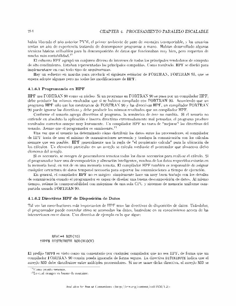
214 CHAPTER 4. PROCESAMIENTO PARALELO ESCALABLE
había liberado el año anterior PVM, el primer ambiente de paso de mensajes transportable, y los usuariostenían un año de experiencia tratando de descomponer programas a mano. Habían desarrollado algunastécnicas básicas utilizables para la descomposición de datos que funcionaban muy bien, pero requerían demucha más contabilidad.12
El esfuerzo HPF agrupó un conjunto diverso de intereses de todos los principales vendedores de cómputode alto rendimiento. Estaban representadas las principales compañías. Como resultado, HPF se diseñó paraimplementarse en casi todo tipo de arquitecturas.
Hay un esfuerzo en marcha para producir el siguiente estándar de FORTRAN, FORTRAN 95, que seespera adopte algunas pero no todas las modi�caciones de HPF.
4.1.6.1 Programando en HPF
HPF usa FORTRAN 90 como su núcleo. Si un programa en FORTRAN 90 se pasa por un compilador HPF,debe producir los mismos resultados que si se hubiera compilado con FORTRAN 90. Asumiendo que unprograma HPF sólo use los constructos de FORTRAN 90 y las directivas HPF, un compilador FORTRAN90 puede ignorar las directivas y debe producir los mismos resultados que un compilador HPF.
Conforme el usuario agrega directivas al programa, la semántica de éste no cambia. Si el usuario noentiende en absoluto la aplicación e inserta directivas extremadamente mal pensadas, el programa produceresultados correctos aunque muy lentamente. Un compilador HPF no trata de "mejorar" las directivas delusuario. Asume que el programador es omniscente.13
Una vez que el usuario ha determinado cómo distribuir los datos entre los procesadores, el compiladorde HPF trata de usar el mínimo de comunicaciones necesario y traslapa la comunicación con los cálculossiempre que sea posible. HPF generalmente usa la regla de "el propietario calcula" para la ubicación delos cálculos. Un elemento particular en un arreglo se calcula mediante el procesador que almacena dichoelemento del arreglo.
Si es necesario, se recogen de procesadores remotos todos los datos necesarios para realizar el cálculo. Siel programador hace una descomposición y alineación inteligentes, muchos de los datos requeridos estarán enla memoria local, en vez de en una memoria remota. El compilador HPF también es responsable de asignarcualquier estructura de datos temporal necesaria para soportar las comunicaciones a tiempo de ejecución.
En general, el compilador HPF no es mágico -simplemente hace un muy buen trabajo con los detallesde comunicación cuando el programador es capaz de diseñar una buena descomposición de datos. Al mismotiempo, retiene la transportabilidad con máquinas de una sola CPU y sistemas de memoria uniforme com-partida usando FORTRAN 90.
4.1.6.2 Directivas HPF de Disposición de Datos
Tal vez las contribuciones más importantes de HPF sean las directivas de disposición de datos. Usándolas,el programador puede controlar cómo se acomodan los datos, basándose en su conocimiento acerca de lasinteracciones entre datos. Una directiva de ejemplo es la que sigue:
REAL*4 ROD(10)
!HPF$ DISTRIBUTE ROD(BLOCK)
El pre�jo !HPF$ es visto como un comentario por cualquier compilador que no sea HPF, de forma que uncompilador FORTRAN 90 común pueda ignorarla de forma segura. La directiva DISTRIBUTE indica que elarreglo ROD debe distribuirse entre múltiples procesadores. Si no se usase dicha directiva, el arreglo ROD se
12Como pronto veremos.13Lo cual siempre es bueno de asumirse.
Available for free at Connexions <http://cnx.org/content/col11356/1.2>
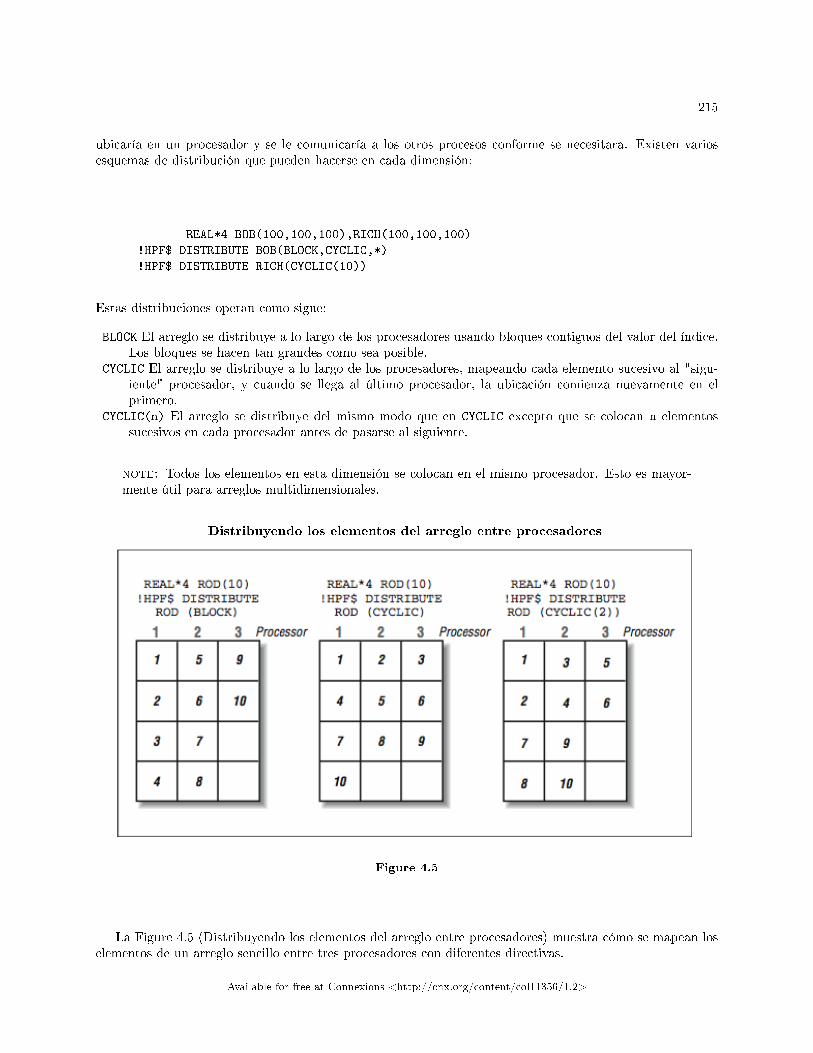
215
ubicaría en un procesador y se le comunicaría a los otros procesos conforme se necesitara. Existen variosesquemas de distribución que pueden hacerse en cada dimensión:
REAL*4 BOB(100,100,100),RICH(100,100,100)
!HPF$ DISTRIBUTE BOB(BLOCK,CYCLIC,*)
!HPF$ DISTRIBUTE RICH(CYCLIC(10))
Estas distribuciones operan como sigue:
BLOCK El arreglo se distribuye a lo largo de los procesadores usando bloques contiguos del valor del índice.Los bloques se hacen tan grandes como sea posible.
CYCLIC El arreglo se distribuye a lo largo de los procesadores, mapeando cada elemento sucesivo al "sigu-iente" procesador, y cuando se llega al último procesador, la ubicación comienza nuevamente en elprimero.
CYCLIC(n) El arreglo se distribuye del mismo modo que en CYCLIC excepto que se colocan n elementossucesivos en cada procesador antes de pasarse al siguiente.
note: Todos los elementos en esta dimensión se colocan en el mismo procesador. Esto es mayor-mente útil para arreglos multidimensionales.
Distribuyendo los elementos del arreglo entre procesadores
Figure 4.5
La Figure 4.5 (Distribuyendo los elementos del arreglo entre procesadores) muestra cómo se mapean loselementos de un arreglo sencillo entre tres procesadores con diferentes directivas.
Available for free at Connexions <http://cnx.org/content/col11356/1.2>
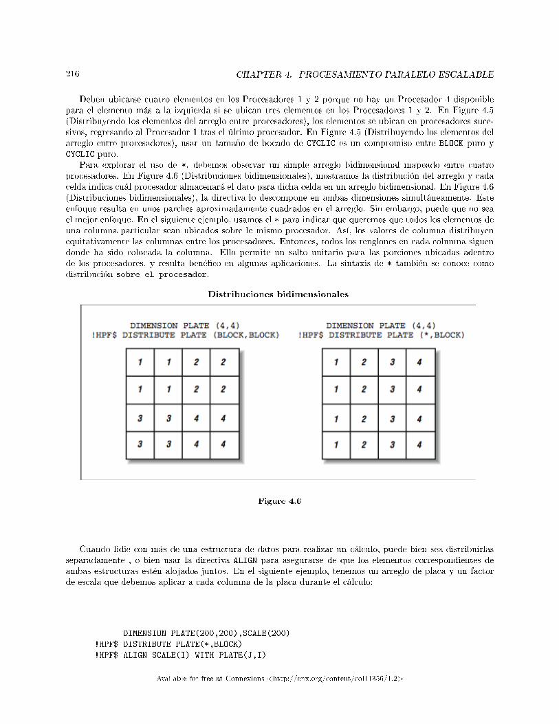
216 CHAPTER 4. PROCESAMIENTO PARALELO ESCALABLE
Deben ubicarse cuatro elementos en los Procesadores 1 y 2 porque no hay un Procesador 4 disponiblepara el elemento más a la izquierda si se ubican tres elementos en los Procesadores 1 y 2. En Figure 4.5(Distribuyendo los elementos del arreglo entre procesadores), los elementos se ubican en procesadores suce-sivos, regresando al Procesador 1 tras el último procesador. En Figure 4.5 (Distribuyendo los elementos delarreglo entre procesadores), usar un tamaño de bocado de CYCLIC es un compromiso entre BLOCK puro yCYCLIC puro.
Para explorar el uso de *, debemos observar un simple arreglo bidimensional mapeado entre cuatroprocesadores. En Figure 4.6 (Distribuciones bidimensionales), mostramos la distribución del arreglo y cadacelda indica cuál procesador almacenará el dato para dicha celda en un arreglo bidimensional. En Figure 4.6(Distribuciones bidimensionales), la directiva lo descompone en ambas dimensiones simultáneamente. Esteenfoque resulta en unos parches aproximadamente cuadrados en el arreglo. Sin embargo, puede que no seael mejor enfoque. En el siguiente ejemplo, usamos el * para indicar que queremos que todos los elementos deuna columna particular sean ubicados sobre le mismo procesador. Así, los valores de columna distribuyenequitativamente las columnas entre los procesadores. Entonces, todos los renglones en cada columna siguendonde ha sido colocada la columna. Ello permite un salto unitario para las porciones ubicadas adentrode los procesadores, y resulta bené�co en algunas aplicaciones. La sintaxis de * también se conoce comodistribución sobre el procesador.
Distribuciones bidimensionales
Figure 4.6
Cuando lidie con más de una estructura de datos para realizar un cálculo, puede bien sea distribuirlasseparadamente , o bien usar la directiva ALIGN para asegurarse de que los elementos correspondientes deambas estructuras estén alojados juntos. En el siguiente ejemplo, tenemos un arreglo de placa y un factorde escala que debemos aplicar a cada columna de la placa durante el cálculo:
DIMENSION PLATE(200,200),SCALE(200)
!HPF$ DISTRIBUTE PLATE(*,BLOCK)
!HPF$ ALIGN SCALE(I) WITH PLATE(J,I)
Available for free at Connexions <http://cnx.org/content/col11356/1.2>
217
O bien:
DIMENSION PLATE(200,200),SCALE(200)
!HPF$ DISTRIBUTE PLATE(*,BLOCK)
!HPF$ ALIGN SCALE(:) WITH PLATE(*,:)
En ambos ejemplos, las variables PLATE y SCALE están ubicadas en los mismos procesadores que las columnascorrespondientes de PLATE. La sintaxis * y : comunican la misma información. Cuando se usa *, esadimensión se colapsa y no participa en la distribución. Cuando se usa :, signi�ca que la esa dimensión siguea la dimensión correspondiente en la variable que ya ha sido distribuida.
También puede usted especi�car el acomodo de la variable SCALE y hacer que la variable PLATE "siga" ladistribución de la variable SCALE:
DIMENSION PLATE(200,200),SCALE(200)
!HPF$ DISTRIBUTE SCALE(BLOCK)
!HPF$ ALIGN PLATE(J,I) WITH SCALE(I)
Puede agregar expresiones aritméticas simples en la directiva ALIGN, sujetas a ciertas limitaciones. Las otrasdirectivas incluyen:
PROCESSORS Le permite crear una forma de con�guración de los procesos que pueda usarse para alinearotras estructuras de datos.
REDISTRIBUTE y REALIGN Le permite cambiar dinámicamente la forma de las estructuras de datos a tiempode ejecución, conforme cambian los patrones de comunicación durante el curso de la misma.
TEMPLATE Le permite crear un arreglo que no usa espacio. En vez de distribuir una estructura de datos yalinear todas las demás, algunos usuarios crearán y distribuirán una plantilla y luego alinearán todaslas estructuras de datos reales de acuerdo a esa plantilla.
El uso de directivas puede �uctuar desde lo muy simple a lo muy complejo. En algunas situaciones, usteddistribuirá la única estructura grande compartida, alineando unas pocas estructuras relacionadas y habráterminado. En otras, los programadores intentan optimizar las comunicaciones basándose en la topología dela red de interconexión (hypercubo, red de interconexión multietapa, malla o toroide) usando directivas muydetalladas. También pueden redistribuir cuidadosamente los datos durante las varias fases del cómputo.
Con suerte, su aplicación logrará un buen rendimiento sin demasiado esfuerzo.
4.1.6.3 Estructuras de control en HPF
Mientras los diseñadores de HPF estaban enmedio de de�nir un nuevo lenguaje, se dieron a la tarea de mejoraraquello que habían visto como una limitación de FORTRAN 90. Es interesante que tales modi�caciones sonlas que se están considerando como parte del nuevo estándar de FORTRAN 95.
La sentencia FORALL permite al usuario expresar operaciones iterativas sencillas que se aplican al arreglocompleto, sin descansar en un ciclo do-loop (recuerde, los ciclos do-loop fuerzan un orden). Por ejemplo:
Available for free at Connexions <http://cnx.org/content/col11356/1.2>
218 CHAPTER 4. PROCESAMIENTO PARALELO ESCALABLE
FORALL (I=1:100, J=1:100) A(I,J) = I + J
Ello puede expresarse en FORTRAN 90 nativo, pero es mucho más feo, contraintuitivo y propenso a errores.Otra estructura de control proporciona la habilidad de declarar una función como "PURE." Una función
PURE no tiene efectos secundarios mas que a través de sus parámetros. El programador garantiza que unafunción PURE puede ejecutarse simultáneamente en muchos procesadores sin efectos indeseables. Esto lepermite a HPF asumir que dicha función sólo operará sobre datos locales y que no requiere de ningunacomunicación de datos durante el tiempo que dure su ejecución completa. El programador también puededeclarar cuáles parámetros de la función son de entrada, cuáles de salida y cuáles de ambos.
4.1.6.4 Intrínsecos de HPF
Las compañías que venden computadoras SIMD requieren entregarlas con herramientas que permitan laejecución de operaciones colectivas e�cientes sobre todos los procesadores. Un ejemplo perfecto de esto es laoperación SUM. Para SUM el valor de un arreglo a lo largo de N procesadores, el enfoque más simplista tomaN pasos. Sin embargo, es posible lograrlo en log(N) pasos usando una técnica denominada suma pre�ja enparalelo. Al momento en que se estaba desarrollando HPF se habían identi�cado e implementado varias detales operaciones. HPF dio la oportunidad de de�nir una sintaxis estandarizada para ellas.
Una muestra de tales operaciones incluye:
SUM_PREFIX Realiza varios tipos de sumas pre�jas en paralelo.ALL_SCATTER Distribuye un único valor a un conjunto de procesadores.GRADE_DOWN Ordena en orden decreciente.IANY Calcula el OR lógico de un conjunto de valores.
Aun cuando existe un gran número de tales funciones intrínsecas, la mayoría de las aplicaciones sólo usaunas pocas de tales operaciones.
4.1.6.5 Extrínsecos de HPF
Con el objeto de permitir a los vendedores de arquitecturas diversas, proporcionar sus ventajas particulares,HPF incluyó la capacidad de enlazarse con funciones "extrínsecas". Tales funciones no requieren de ree-scribirse en FORTRAN 90/HPF, y realizan varias capacidades sólo soportadas por los vendedores. Estacapacidad permite a los usuarios realizar tales tareas, como la creación de aplicaciones híbridas, con algo deHPF y algo de paso de mensajes.
Los programadores de cómputo de alto rendimiento siempre gustan de tener la habilidad de hacer cosasa su propio modo, con el objetivo de exprimir hasta la última gota de rendimiento.
4.1.6.6 Flujo Calórico en HPF
Para transportar nuestra aplicación de �ujo calórico a HPF, realmente sólo requerimos de agregar una líneade código. En el ejemplo siguiente, lo hemos cambiado a un arreglo bidimensional más grande:
INTEGER PLATESIZ,MAXTIME
PARAMETER(PLATESIZ=2000,MAXTIME=200)
!HPF$ DISTRIBUTE PLATE(*,BLOCK)
REAL*4 PLATE(PLATESIZ,PLATESIZ)
Available for free at Connexions <http://cnx.org/content/col11356/1.2>
219
INTEGER TICK
PLATE = 0.0
* Sumar las fronteras
PLATE(1,:) = 100.0
PLATE(PLATESIZ,:) = -40.0
PLATE(:,PLATESIZ) = 35.23
PLATE(:,1) = 4.5
DO TICK = 1,MAXTIME
PLATE(2:PLATESIZ-1,2:PLATESIZ-1) = (
+ PLATE(1:PLATESIZ-2,2:PLATESIZ-1) +
+ PLATE(3:PLATESIZ-0,2:PLATESIZ-1) +
+ PLATE(2:PLATESIZ-1,1:PLATESIZ-2) +
+ PLATE(2:PLATESIZ-1,3:PLATESIZ-0) ) / 4.0
PRINT 1000,TICK, PLATE(2,2)
1000 FORMAT('TICK = ',I5, F13.8)
ENDDO
*
END
Notará que la directiva HPF distribuye las columnas del arreglo usando el enfoque BLOCK, manteniendotodos los elementos de una columna sobre un mismo procesador. A primera vista, pudiera parecer que(BLOCK,BLOCK) es la mejor distribución. Sin embargo, hay dos ventajas de una distribución (*,BLOCK).Primero, recorrer hacia abajo una columna es una operación de paso único, y de este modo puede ustedprocesar una columna completa. El aspecto más signi�cativo de la distribución es que una distribución(BLOCK,BLOCK) fuerza a cada procesador a comunicarse con hasta ocho procesadores más para obtener losvalores de sus vecinos. Usando la distribución (*,BLOCK), cada procesador tendrá que intercambiar datos concuando mucho dos procesadores en cada ciclo.
Cuando veamos PVM, veremos el mismo programa implementado al estilo de paso de mensajes SPMD.En este ejemplo, verá usted algunos de los detalles que HFP debe manejar para ejecutar apropiadamenteeste código. Tras revisarlo ½probablemente usted elija implementar todas sus aplicaciones futuras de �ujocalórico en HPF!
4.1.6.7 Resumen de HPF
En ciertas cosas HPF ha sido mejor que FORTRAN 90. Compañías como IBM con su SP-1 requierende proporcionar algún lenguaje de alto nivel para el que sus usuarios no quieren escribir código de pasode mensajes. Por tal motivo, IBM ha invertido una gran cantidad de esfuerzo en implementar un HPFoptimizado. Resulta interesante que mucho de su esfuerzo bene�ciará directamente la habilidad de desarrollarcompiladores de FORTRAN 90 más so�sticados. El extensivo análisis de �ujo de datos requerido paraminimizar las comunicaciones y administrar las estructuras de datos dinámicos recaerá en los compiladoresde FORTRAN 90 incluso sin usar las directivas de HPF.
El tiempo dirá si ya no serán necesarias las directivas de distribución de datos de HPF, y si los compi-ladores serán capaces de realizar su�ciente análisis sobre el código plano de FORTRAN 90 para optimizarla ubicación y movimiento de los datos.
En su forma actual, HPF es un vehículo excelente para expresar las aplicaciones altamente paralelas anivel de datos, y basadas en retículas. Sus debilidades son las comunicaciones irregulares y el balance decargas dinámicas. Un nuevo esfuerzo para desarrollar la siguiente versión de HPF está en camino, paramanejar algunos de estos temas. Desafortunadamente, es más difícil resolver estos problemas a tiempo deejecución a la vez que se mantiene un buen rendimiento a través de una amplia variedad de arquitecturas.
Available for free at Connexions <http://cnx.org/content/col11356/1.2>

220 CHAPTER 4. PROCESAMIENTO PARALELO ESCALABLE
4.1.7 Soporte del Lenguaje para Mejorar el Rendimiento - Notas Finales14
En este capítulo, hemos cubierto algunos de los esfuerzos que se han desarrollado en el área de los lenguajespara permitir la escritura de programas para cómputo escalable. Existe una pugna entre el FORTRAN-77puro, el FORTRAN 90, el HPF y el paso de mensajes por convertirse en la herramienta de�nitiva para elcómputo escalable de alto rendimiento.
Ciertamente, ha habido ejemplos de grandes éxitos tanto de FORTRAN 90 (Thinking Machines CM-5)y HPF (IBM SP y otros) como lenguajes que pueden hacer un excelente uso de los sistemas de cómputoescalables. Uno de los problemas del enfoque basado en lenguajes de alto nivel es que, en algunas ocasiones,usar un lenguaje de alto nivel abstracto en realidad reduce la transportabilidad efectiva.
Los lenguajes están diseñados para ser transportables, pero si el vendedor de su computadora escalableparticular no suporte la variante de lenguaje en la que usted ha elegido escribir su aplicación, entonces no serátransportable. Incluso si el vendedor tiene disponible su lenguaje, puede que no esté a�nado para generar elmejor código para su arquitectura.
Una solución estriba en comprar sus compiladores de una tercer compañía, tal como Paci�c Sierra o Kucky Asociados. Estos vendedores comercializan un compilador que se ejecuto sobre un amplio rango de sistema.Para aquellos usuarios que puedan costear tales opciones, estos compiladores proporcionan un mayor nivelde transportabilidad.
Una de las preocupaciones fundamentales es el problema del huevo y la gallina. Si los usuarios no empleanun lenguaje, los vendedores no le harán mejoras. Si todos los usuarios in�uyentes (con todo el dinero) usanpaso de mensajes, entonces la existencia de un compilador excelente de HPF no tiene ningún valor real paraesos usuarios.
Las buenas noticias son que tanto FORTRAN 90 como HPF proporcionan un camino hacia el cómputoescalable transportable que no requiere paso de mensajes explícito. La única pregunta es qué camino decidiránusar los usuarios.
4.2 Ambientes de Paso de Mensajes
4.2.1 Ambientes de Paso de Mensajes - Introducción15
Una interfaz de paso de mensajes es un conjunto de funciones y llamados a subrutinas para C o FORTRAN,que le proporcionan una forma de dividir una aplicación para que pueda ejecutarse en paralelo. Los datosse dividen y pasan a otros procesadores en forma de mensajes. Los procesadores receptores los desem-pacan, realizan algún trabajo, y envían los resultados de vuelta, o bien los pasan a otros procesadores en lacomputadora paralela.
En cierta forma, el paso de mensajes es el "lenguaje ensamblador" del procesamiento paralelo. Cargasobre sus hombros la responsabilidad última, y si usted es talentoso (y el problema que trata de resolvercoopera), le permite lograr el máximo rendimiento. Si tiene usted un problema fácilmente escalable y noestá satisfecho con el rendimiento obtenido, muy probablemente sea su culpa, puesto que el compilador nosabe nada de los aspectos paralelos del programa.
Los dos ambientes de paso de mensajes más populares son parallel virtual machine (PVM) y message-passing interface (MPI). Muchas de las características importantes están disponibles en ambos ambientes.Una vez que se haya convertido en un experto en paso de mensajes, migrar de PVM a MPI no le dará prob-lemas. Incluso podrá usted operar sobre un sistema que proporcione sólo una interfaz de paso de mensajespropietaria. Sin embargo, una vez que entienda los conceptos de paso de mensajes y haya descompuestoapropiadamente su aplicación, usualmente no le costará mucho más migrarlo de una biblioteca de paso demensajes a otra.16
14This content is available online at <http://cnx.org/content/m38337/1.1/>.15This content is available online at <http://cnx.org/content/m38292/1.2/>.16Note que dije "no le costará mucho más.�
Available for free at Connexions <http://cnx.org/content/col11356/1.2>
221
4.2.2 Ambientes de Paso de Mensajes - Parallel Virtual Machine17
La idea tras PVM consiste en ensamblar una "máquina virtual" mediante un conjunto diverso de recursosenlazados por una red. Un usuario puede controlar los recursos de 35 estaciones disponibles sobre la Internet,y tener su propio sistema de procesamiento escalable. El trabajo de PVM comenzó a inicios de la década de1990 en Oak Ridge National Labs, y en buena medida se convirtió en un éxito instantáneo en la comunidadcientí�ca. Proporciona un marco de trabajo en bruto que permite experimentar con el uso de redes deestaciones de trabajo como procesadores paralelos.
En PVM versión 3, puede usted crear su máquina virtual usando procesadores individuales, multiproce-sadores de memoria compartida y multiprocesadores escalables. PVM intenta entretejer todos esos recursosen un ambiente de ejecución único y consistente.
Para ejecutar PVM, lo único que requiere usted es una cuenta de acceso en un conjunto de computadorasen red, que tengan instalado el software PVM. Incluso puede usted instalarlo en su propio directorio personal.Para crear su propia máquina virtual personal, debe integrar una lista de tales computadoras en un archivo:
% cat hostfile
frodo.egr.msu.edu
gollum.egr.msu.edu
mordor.egr.msu.edu
%
Tras ciertas manipulaciones no triviales de rutas de acceso y variables de ambiente, puede usted arrancar laconsola PVM:
% pvm hostfile
pvmd already running.
pvm> conf
1 host, 1 data format
HOST DTID ARCH SPEED
frodo 40000 SUN4SOL2 1000
gollum 40001 SUN4SOL2 1000
mordor 40002 SUN4SOL2 1000
pvm> ps
HOST TID FLAG 0x COMMAND
frodo 40042 6/c,f pvmgs
pvm> reset
pvm> ps
HOST TID FLAG 0x COMMAND
pvm>
Muchos usuarios distintos puede ejecutar máquinas virtuales que usan el mismo grupo de recursos. Y cadausuario a ver como una máquina vacía. La única forma de que detecte usted las otras máquinas virtuales queemplean los mismos recursos que la suya, es mediante el porcentaje de tiempo que sus aplicaciones tendránel control de la CPU.
17This content is available online at <http://cnx.org/content/m38291/1.1/>.
Available for free at Connexions <http://cnx.org/content/col11356/1.2>
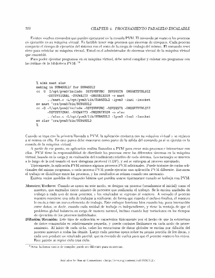
222 CHAPTER 4. PROCESAMIENTO PARALELO ESCALABLE
Existen muchos comandos que pueden ejecutarse en la consola PVM. El comando ps muestra los procesosen ejecución en su máquina virtual. Es factible tener más procesos que sistemas de cómputo. Cada procesocomparte el tiempo de ejecución del sistema con el resto de la carga de trabajo del mismo. El comando resetsirve para reiniciar su máquina virtual. Usted es el administrador de sistemas virtual de la máquina virtualque ensambló.
Para poder ejecutar programas en su máquina virtual, debe usted compilar y enlazar sus programas conlas rutinas de la biblioteca PVM: 18
% aimk mast slav
making in SUN4SOL2/ for SUN4SOL2
cc -O -I/opt/pvm3/include -DSYSVBFUNC -DSYSVSTR -DNOGETDTBLSIZ
-DSYSVSIGNAL -DNOWAIT3 -DNOUNIXDOM -o mast
../mast.c -L/opt/pvm3/lib/SUN4SOL2 -lpvm3 -lnsl -lsocket
mv mast �crs/pvm3/bin/SUN4SOL2
cc -O -I/opt/pvm3/include -DSYSVBFUNC -DSYSVSTR -DNOGETDTBLSIZ
-DSYSVSIGNAL -DNOWAIT3 -DNOUNIXDOM -o slav
../slav.c -L/opt/pvm3/lib/SUN4SOL2 -lpvm3 -lnsl -lsocket
mv slav �crs/pvm3/bin/SUN4SOL2
%
Cuando se topa con la primera llamada a PVM, la aplicación contacta con su máquina virtual y se registraa sí misma en ella. En este punto debe mostrarse como parte de la salida del comando ps si se ejecuta en laconsola de la máquina virtual.
A partir de ese punto, su aplicación realiza llamadas a PVM para crear más procesos e interactuar conellos. PVM tiene la responsabilidad de distribuir los procesos entre los diferentes sistemas en la máquinavirtual, basado en la carga y su evaluación del rendimiento relativo de cada sistema. Los mensajes se muevena lo largo de la red usando el user datagram protocol (UDP), y así se entregan al proceso apropiado.
Típicamente, la aplicación PVM arranca algunos procesos PVM adicionales. Puede tratarse de copias adi-cionales del mismo programa, o cada proceso PVM puede ejecutar una aplicación PVM diferente. Entoncesel trabajo se distribuye entre los procesos, y los resultados se reúnen cuando sea necesario.
Existen varios modelos de cómputo básicos que pueden usarse típicamente cuando se trabaja con PVM:
Maestro/Esclavo: Cuando se opera en este modo, se designa un proceso (usualmente el inicial) como elmaestro, que engendra cierto número de procesos que realizarán el trabajo. Se le envían unidades detrabajo a cada uno de estos procesos, y los resultados se regresan al maestro. A menudo el procesomaestro mantiene una cola de trabajos a realizarse, de forma que cuando el esclavo �naliza, el maestrole envía a éste un nuevo elemento de trabajo. Este enfoque funciona bien cuando hay poca interacciónentre datos, es decir, cuando cada unidad de trabajo es independiente, y tiene la ventaja de que elproblema global balancea su carga de manera natural, incluso cuando hay variaciones en los tiemposde ejecución de los procesos individuales.
Difusión/Reunión: Este tipo de aplicación se caracteriza típicamente por el hecho de que la estructurade datos compartida es relativamente pequeña, y puede copiarse fácilmente en cada nodo de proce-samiento. Al inicio de cada ciclo, todas las estructuras de datos globales se envían por difusión delproceso maestro a todos los demás. Luego cada proceso opera sobre su propia porción de los datos, ycada uno produce un resultado parcial, que es enviado de vuelta para que el proceso maestro los reúna.Este patrón se repite ciclo tras ciclo.
18Nota: la forma exacta de compilar puede ser diferente para su sistema.
Available for free at Connexions <http://cnx.org/content/col11356/1.2>
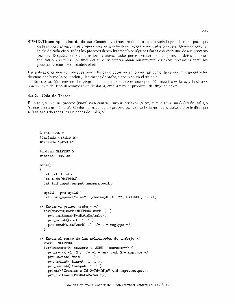
223
SPMD/Descomposición de datos: Cuando la estructura de datos es demasiado grande como para quecada proceso almacena su propia copia, ésta debe dividirse entre múltiples procesos. Generalmente, alinicio de cada ciclo, todos los procesos deben intercambiar algunos datos con cada uno de sus procesosvecinos. Después, con sus datos locales acrecentados por el necesario subconjunto de datos remotos,realizan sus cáculos. Al �nal del ciclo, se intercambian nuevamente los datos necesarios entre losprocesos vecinos, y se reinicia el ciclo.
Las aplicaciones mas complicadas tienen �ujos de datos no uniformes, así como datos que migran entre lossistemas conforme la aplicación y las cargas de trabajo cambian en el sistema.
En esta sección tenemos dos programas de ejemplo: uno es una operación maestro-esclavo, y la otra esuna solución del tipo descomposición de datos, ambos para el problema del �ujo de calor.
4.2.2.1 Cola de Tareas
En este ejemplo, un proceso (mast) crea cuatro procesos esclavos (slav) y reparte 20 unidades de trabajo(sumar uno a un número). Conforme responde un proceso esclavo, se le da un nuevo trabajo o se le dice quese han agotado todas las unidades de trabajo:
% cat mast.c
#include <stdio.h>#include "pvm3.h"
#define MAXPROC 5
#define JOBS 20
main()
{
int mytid,info;
int tids[MAXPROC];
int tid,input,output,answers,work;
mytid = pvm_mytid();
info=pvm_spawn("slav", (char**)0, 0, "", MAXPROC, tids);
/* Envía el primer trabajo */
for(work=0;work<MAXPROC;work++) {
pvm_initsend(PvmDataDefault);
pvm_pkint(&work, 1, 1 ) ;
pvm_send(tids[work],1) ;/* 1 = msgtype */
}
/* Envía el resto de las solicitudes de trabajo */
work = MAXPROC;
for(answers=0; answers < JOBS ; answers++) {
pvm_recv( -1, 2 ); /* -1 = any task 2 = msgtype */
pvm_upkint( &tid, 1, 1 );
pvm_upkint( &input, 1, 1 );
pvm_upkint( &output, 1, 1 );
printf("Gracias a %d 2*%d=%d\n",tid,input,output);pvm_initsend(PvmDataDefault);
Available for free at Connexions <http://cnx.org/content/col11356/1.2>
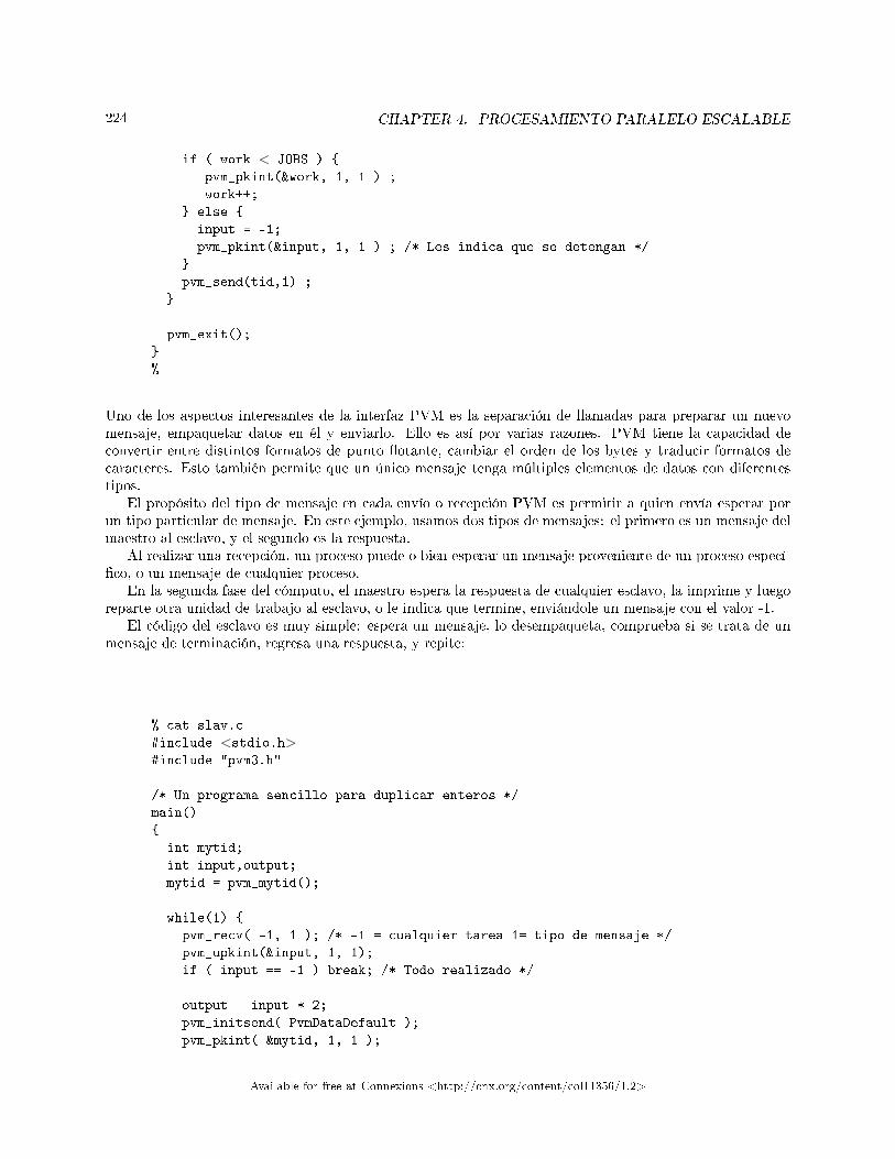
224 CHAPTER 4. PROCESAMIENTO PARALELO ESCALABLE
if ( work < JOBS ) {
pvm_pkint(&work, 1, 1 ) ;
work++;
} else {
input = -1;
pvm_pkint(&input, 1, 1 ) ; /* Les indica que se detengan */
}
pvm_send(tid,1) ;
}
pvm_exit();
}
%
Uno de los aspectos interesantes de la interfaz PVM es la separación de llamadas para preparar un nuevomensaje, empaquetar datos en él y enviarlo. Ello es así por varias razones. PVM tiene la capacidad deconvertir entre distintos formatos de punto �otante, cambiar el orden de los bytes y traducir formatos decaracteres. Esto también permite que un único mensaje tenga múltiples elementos de datos con diferentestipos.
El propósito del tipo de mensaje en cada envío o recepción PVM es permitir a quien envía esperar porun tipo particular de mensaje. En este ejemplo, usamos dos tipos de mensajes: el primero es un mensaje delmaestro al esclavo, y el segundo es la respuesta.
Al realizar una recepción, un proceso puede o bien esperar un mensaje proveniente de un proceso especí-�co, o un mensaje de cualquier proceso.
En la segunda fase del cómputo, el maestro espera la respuesta de cualquier esclavo, la imprime y luegoreparte otra unidad de trabajo al esclavo, o le indica que termine, enviándole un mensaje con el valor -1.
El código del esclavo es muy simple: espera un mensaje, lo desempaqueta, comprueba si se trata de unmensaje de terminación, regresa una respuesta, y repite:
% cat slav.c
#include <stdio.h>#include "pvm3.h"
/* Un programa sencillo para duplicar enteros */
main()
{
int mytid;
int input,output;
mytid = pvm_mytid();
while(1) {
pvm_recv( -1, 1 ); /* -1 = cualquier tarea 1= tipo de mensaje */
pvm_upkint(&input, 1, 1);
if ( input == -1 ) break; /* Todo realizado */
output = input * 2;
pvm_initsend( PvmDataDefault );
pvm_pkint( &mytid, 1, 1 );
Available for free at Connexions <http://cnx.org/content/col11356/1.2>
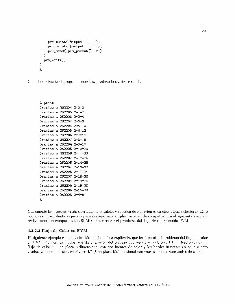
225
pvm_pkint( &input, 1, 1 );
pvm_pkint( &output, 1, 1 );
pvm_send( pvm_parent(), 2 );
}
pvm_exit();
}
%
Cuando se ejecuta el programa maestro, produce la siguiente salida:
% pheat
Gracias a 262204 2*0=0
Gracias a 262205 2*1=2
Gracias a 262206 2*2=4
Gracias a 262207 2*3=6
Gracias a 262204 2*5=10
Gracias a 262205 2*6=12
Gracias a 262206 2*7=14
Gracias a 262207 2*8=16
Gracias a 262204 2*9=18
Gracias a 262205 2*10=20
Gracias a 262206 2*11=22
Gracias a 262207 2*12=24
Gracias a 262205 2*14=28
Gracias a 262207 2*16=32
Gracias a 262205 2*17=34
Gracias a 262207 2*18=36
Gracias a 262204 2*13=26
Gracias a 262205 2*19=38
Gracias a 262206 2*15=30
Gracias a 262208 2*4=8
%
Claramente los procesos están operando en paralelo, y el orden de ejecución es en cierta forma eleatorio. Estecódigo es un excelente esqueleto para manejar una amplia variedad de cómputos. En el siguiente ejemplo,realizaremos un cómputo estilo SPMD para resolver el problema del �ujo de calor usando PVM.
4.2.2.2 Flujo de Calor en PVM
El siguiente ejemplo es una aplicación mucho más complicada, que implementa el problema del �ujo de caloren PVM. De muchos modos, nos da una vsión del trabajo que realiza el ambiente HPF. Resolveremos un�ujo de calor en una placa bidimensional con dos fuentes de calor y los bordes inmersos en agua a cerogrados, como se muestra en Figure 4.7 (Una placa bidimensional con cuatro fuentes constantes de calor).
Available for free at Connexions <http://cnx.org/content/col11356/1.2>
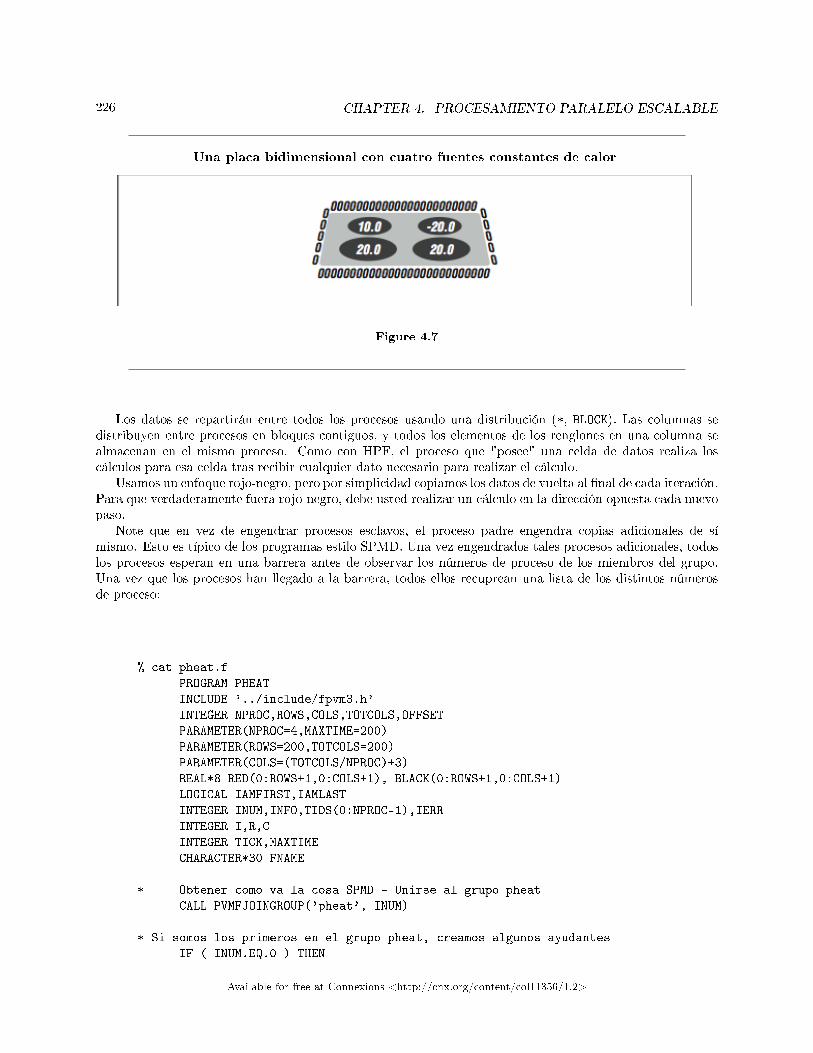
226 CHAPTER 4. PROCESAMIENTO PARALELO ESCALABLE
Una placa bidimensional con cuatro fuentes constantes de calor
Figure 4.7
Los datos se repartirán entre todos los procesos usando una distribución (*, BLOCK). Las columnas sedistribuyen entre procesos en bloques contiguos, y todos los elementos de los renglones en una columna sealmacenan en el mismo proceso. Como con HPF, el proceso que "posee" una celda de datos realiza loscálculos para esa celda tras recibir cualquier dato necesario para realizar el cálculo.
Usamos un enfoque rojo-negro, pero por simplicidad copiamos los datos de vuelta al �nal de cada iteración.Para que verdaderamente fuera rojo-negro, debe usted realizar un cálculo en la dirección opuesta cada nuevopaso.
Note que en vez de engendrar procesos esclavos, el proceso padre engendra copias adicionales de símismo. Esto es típico de los programas estilo SPMD. Una vez engendrados tales procesos adicionales, todoslos procesos esperan en una barrera antes de observar los números de proceso de los miembros del grupo.Una vez que los procesos han llegado a la barrera, todos ellos recuprean una lista de los distintos númerosde proceso:
% cat pheat.f
PROGRAM PHEAT
INCLUDE '../include/fpvm3.h'
INTEGER NPROC,ROWS,COLS,TOTCOLS,OFFSET
PARAMETER(NPROC=4,MAXTIME=200)
PARAMETER(ROWS=200,TOTCOLS=200)
PARAMETER(COLS=(TOTCOLS/NPROC)+3)
REAL*8 RED(0:ROWS+1,0:COLS+1), BLACK(0:ROWS+1,0:COLS+1)
LOGICAL IAMFIRST,IAMLAST
INTEGER INUM,INFO,TIDS(0:NPROC-1),IERR
INTEGER I,R,C
INTEGER TICK,MAXTIME
CHARACTER*30 FNAME
* Obtener como va la cosa SPMD - Unirse al grupo pheat
CALL PVMFJOINGROUP('pheat', INUM)
* Si somos los primeros en el grupo pheat, creamos algunos ayudantes
IF ( INUM.EQ.0 ) THEN
Available for free at Connexions <http://cnx.org/content/col11356/1.2>
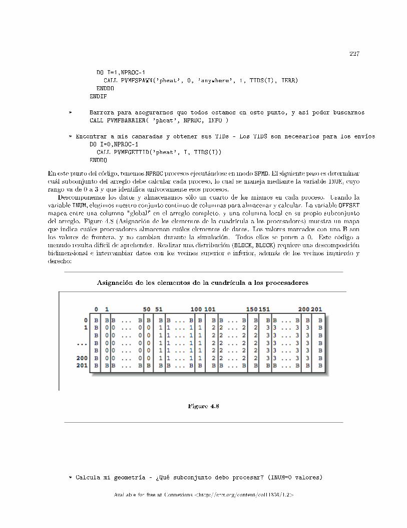
227
DO I=1,NPROC-1
CALL PVMFSPAWN('pheat', 0, 'anywhere', 1, TIDS(I), IERR)
ENDDO
ENDIF
* Barrera para asegurarnos que todos estamos en este punto, y así poder buscarnos
CALL PVMFBARRIER( 'pheat', NPROC, INFO )
* Encontrar a mis camaradas y obtener sus TIDs - Los TIDS son necesarios para los envíos
DO I=0,NPROC-1
CALL PVMFGETTID('pheat', I, TIDS(I))
ENDDO
En este punto del código, tenemos NPROC procesos ejecutándose en modo SPMD. El siguiente paso es determinarcuál subconjunto del arreglo debe calcular cada proceso, lo cual se maneja mediante la variable INUM, cuyorango va de 0 a 3 y que identi�ca unívocamente esos procesos.
Descomponemos los datos y almacenamos sólo un cuarto de los mismos en cada proceso. Usando lavariable INUM, elegimos nuestro conjunto continuo de columnas para almacenar y calcular. La variable OFFSETmapea entre una columna "global" en el arreglo completo, y una columna local en su propio subconjuntodel arreglo. Figure 4.8 (Asignación de los elementos de la cuadrícula a los procesadores) muestra un mapaque indica cuáles procesadores almacenan cuáles elementos de datos. Los valores marcados con una B sonlos valores de frontera, y no cambian durante la simulación. Todos ellos se ponen a 0. Este código amenudo resulta difícil de aprehender. Realizar una distribución (BLOCK, BLOCK) requiere una descomposiciónbidimensional e intercambiar datos con los vecinos superior e inferior, además de los vecinos izquierdo yderecho:
Asignación de los elementos de la cuadrícula a los procesadores
Figure 4.8
* Calcula mi geometría - ¾Qué subconjunto debo procesar? (INUM=0 valores)
Available for free at Connexions <http://cnx.org/content/col11356/1.2>
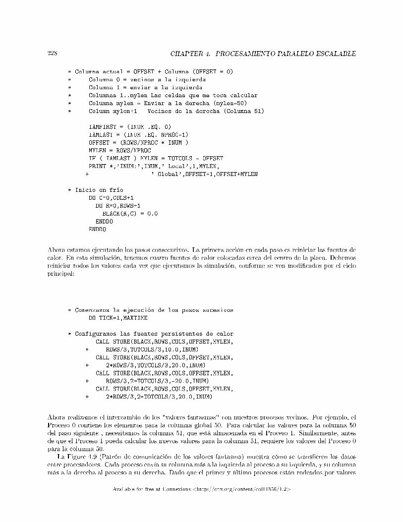
228 CHAPTER 4. PROCESAMIENTO PARALELO ESCALABLE
* Columna actual = OFFSET + Columna (OFFSET = 0)
* Columna 0 = vecinos a la izquierda
* Columna 1 = enviar a la izquierda
* Columnas 1..mylen Las celdas que me toca calcular
* Columna mylen = Enviar a la derecha (mylen=50)
* Column mylen+1 = Vecinos de la derecha (Columna 51)
IAMFIRST = (INUM .EQ. 0)
IAMLAST = (INUM .EQ. NPROC-1)
OFFSET = (ROWS/NPROC * INUM )
MYLEN = ROWS/NPROC
IF ( IAMLAST ) MYLEN = TOTCOLS - OFFSET
PRINT *,'INUM:',INUM,' Local',1,MYLEN,
+ ' Global',OFFSET+1,OFFSET+MYLEN
* Inicio en frío
DO C=0,COLS+1
DO R=0,ROWS+1
BLACK(R,C) = 0.0
ENDDO
ENDDO
Ahora estamos ejecutando los pasos consecutivos. La primera acción en cada paso es reiniciar las fuentes decalor. En esta simulación, tenemos cuatro fuentes de calor colocadas cerca del centro de la placa. Debemosreiniciar todos los valores cada vez que ejecutamos la simulación, conforme se ven modi�cados por el cicloprincipal:
* Comenzamos la ejecución de los pasos sucesivos
DO TICK=1,MAXTIME
* Configuramos las fuentes persistentes de calor
CALL STORE(BLACK,ROWS,COLS,OFFSET,MYLEN,
+ ROWS/3,TOTCOLS/3,10.0,INUM)
CALL STORE(BLACK,ROWS,COLS,OFFSET,MYLEN,
+ 2*ROWS/3,TOTCOLS/3,20.0,INUM)
CALL STORE(BLACK,ROWS,COLS,OFFSET,MYLEN,
+ ROWS/3,2*TOTCOLS/3,-20.0,INUM)
CALL STORE(BLACK,ROWS,COLS,OFFSET,MYLEN,
+ 2*ROWS/3,2*TOTCOLS/3,20.0,INUM)
Ahora realizamos el intercambio de los "valores fantasmas" con nuestros procesos vecinos. Por ejemplo, elProceso 0 contiene los elementos para la columna global 50. Para calcular los valores para la columna 50del paso siguiente , necesitamos la columna 51, que está almacenada en el Proceso 1. Similarmente, antesde que el Proceso 1 pueda calcular los nuevos valores para la columna 51, requiere los valores del Proceso 0para la columna 50.
La Figure 4.9 (Patrón de comunicación de los valores fantasma) muestra cómo se trans�eren los datosentre procesadores. Cada proceso envía su columna más a la izquierda al proceso a su izquierda, y su columnamás a la derecha al proceso a su derecha. Dado que el primer y último procesos están rodeados por valores
Available for free at Connexions <http://cnx.org/content/col11356/1.2>
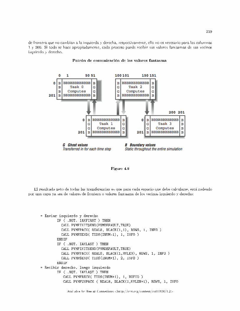
229
de frontera que no cambian a la izquierda y derecha, respectivamente, ello no es necesario para las columnas1 y 200. Si todo se hace apropiadamente, cada proceso puede recibir sus valores fantasmas de sus vecinosizquierdo y derecho.
Patrón de comunicación de los valores fantasma
Figure 4.9
El resultado neto de todas las transferencias es que para cada espacio que debe calcularse, está rodeadopor una capa ya sea de valores de frontera o valores fantasma de los vecinos izquierdo y derecho:
* Enviar izquierdo y derecho
IF ( .NOT. IAMFIRST ) THEN
CALL PVMFINITSEND(PVMDEFAULT,TRUE)
CALL PVMFPACK( REAL8, BLACK(1,1), ROWS, 1, INFO )
CALL PVMFSEND( TIDS(INUM-1), 1, INFO )
ENDIF
IF ( .NOT. IAMLAST ) THEN
CALL PVMFINITSEND(PVMDEFAULT,TRUE)
CALL PVMFPACK( REAL8, BLACK(1,MYLEN), ROWS, 1, INFO )
CALL PVMFSEND( TIDS(INUM+1), 2, INFO )
ENDIF
* Recibir derecho, luego izquierdo
IF ( .NOT. IAMLAST ) THEN
CALL PVMFRECV( TIDS(INUM+1), 1, BUFID )
CALL PVMFUNPACK ( REAL8, BLACK(1,MYLEN+1), ROWS, 1, INFO
Available for free at Connexions <http://cnx.org/content/col11356/1.2>

230 CHAPTER 4. PROCESAMIENTO PARALELO ESCALABLE
ENDIF
IF ( .NOT. IAMFIRST ) THEN
CALL PVMFRECV( TIDS(INUM-1), 2, BUFID )
CALL PVMFUNPACK ( REAL8, BLACK(1,0), ROWS, 1, INFO)
ENDIF
El siguiente segmento es la parte fácil. Todos los valores fantasma apropiados están en su lugar, así quesimplemente debemos realizar el cálculo de nuestro subespacio. Al �nal, copiamos de vuelta desde el arregloROJO al arreglo NEGRO; en una simulación real, podemos realizar dos pasos consecutivos, uno desde NEGRO
hacia ROJO y el otro de ROJO hacia NEGRO, para ahorrar esta copia extra:
* Realiza el flujo
DO C=1,MYLEN
DO R=1,ROWS
RED(R,C) = ( BLACK(R,C) +
+ BLACK(R,C-1) + BLACK(R-1,C) +
+ BLACK(R+1,C) + BLACK(R,C+1) ) / 5.0
ENDDO
ENDDO
* Copia de vuelta - Normalmente haríamos una versión roja y una negra de este ciclo
DO C=1,MYLEN
DO R=1,ROWS
BLACK(R,C) = RED(R,C)
ENDDO
ENDDO
ENDDO
Ahora encontramos la celda central y la enviamos al proceso maestro (si es necesario) de forma que puedaimprimirse. También volcamos los datos en archivos para depuración o visualización posterior de los resul-tados. Cada archivo se hace único agregando a su nombre el número de instancia. Después el programatermina:
CALL SENDCELL(RED,ROWS,COLS,OFFSET,MYLEN,INUM,TIDS(0),
+ ROWS/2,TOTCOLS/2)
* Volcado de los datos para verificación
IF ( ROWS .LE. 20 ) THEN
FNAME = '/tmp/pheatout.' // CHAR(ICHAR('0')+INUM)
OPEN(UNIT=9,NAME=FNAME,FORM='formatted')
DO C=1,MYLEN
WRITE(9,100)(BLACK(R,C),R=1,ROWS)
100 FORMAT(20F12.6)
ENDDO
CLOSE(UNIT=9)
Available for free at Connexions <http://cnx.org/content/col11356/1.2>
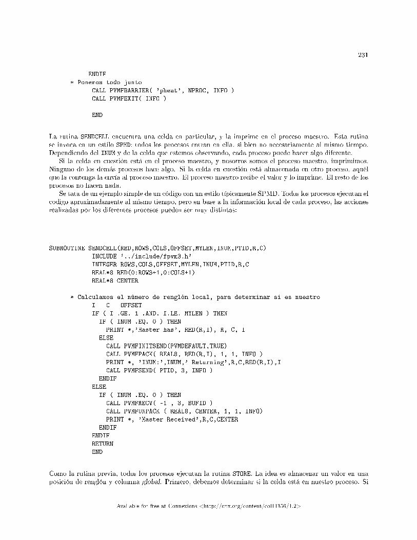
231
ENDIF
* Ponemos todo junto
CALL PVMFBARRIER( 'pheat', NPROC, INFO )
CALL PVMFEXIT( INFO )
END
La rutina SENDCELL encuentra una celda en particular, y la imprime en el proceso maestro. Esta rutinase invoca en un estilo SPMD: todos los procesos entran en ella, si bien no necesariamente al mismo tiempo.Dependiendo del INUM y de la celda que estemos observando, cada proceso puede hacer algo diferente.
Si la celda en cuestión está en el proceso maestro, y nosotros somos el proceso maestro, imprimimos.Ninguno de los demás procesos hace algo. Si la celda en cuestión está almacenada en otro proceso, aquélque la contenga la envía al proceso maestro. El proceso maestro recibe el valor y lo imprime. El resto de losprocesos no hacen nada.
Se tata de un ejemplo simple de un código con un estilo típicamente SPMD. Todos los procesos ejecutan elcodigo aproximadamente al mismo tiempo, pero en base a la información local de cada proceso, las accionesrealizadas por los diferentes procesos pueden ser muy distintas:
SUBROUTINE SENDCELL(RED,ROWS,COLS,OFFSET,MYLEN,INUM,PTID,R,C)
INCLUDE '../include/fpvm3.h'
INTEGER ROWS,COLS,OFFSET,MYLEN,INUM,PTID,R,C
REAL*8 RED(0:ROWS+1,0:COLS+1)
REAL*8 CENTER
* Calculamos el número de renglón local, para determinar si es nuestro
I = C - OFFSET
IF ( I .GE. 1 .AND. I.LE. MYLEN ) THEN
IF ( INUM .EQ. 0 ) THEN
PRINT *,'Master has', RED(R,I), R, C, I
ELSE
CALL PVMFINITSEND(PVMDEFAULT,TRUE)
CALL PVMFPACK( REAL8, RED(R,I), 1, 1, INFO )
PRINT *, 'INUM:',INUM,' Returning',R,C,RED(R,I),I
CALL PVMFSEND( PTID, 3, INFO )
ENDIF
ELSE
IF ( INUM .EQ. 0 ) THEN
CALL PVMFRECV( -1 , 3, BUFID )
CALL PVMFUNPACK ( REAL8, CENTER, 1, 1, INFO)
PRINT *, 'Master Received',R,C,CENTER
ENDIF
ENDIF
RETURN
END
Como la rutina previa, todos los procesos ejecutan la rutina STORE. La idea es almacenar un valor en unaposición de renglón y columna global. Primero, debemos determinar si la celda está en nuestro proceso. Si
Available for free at Connexions <http://cnx.org/content/col11356/1.2>
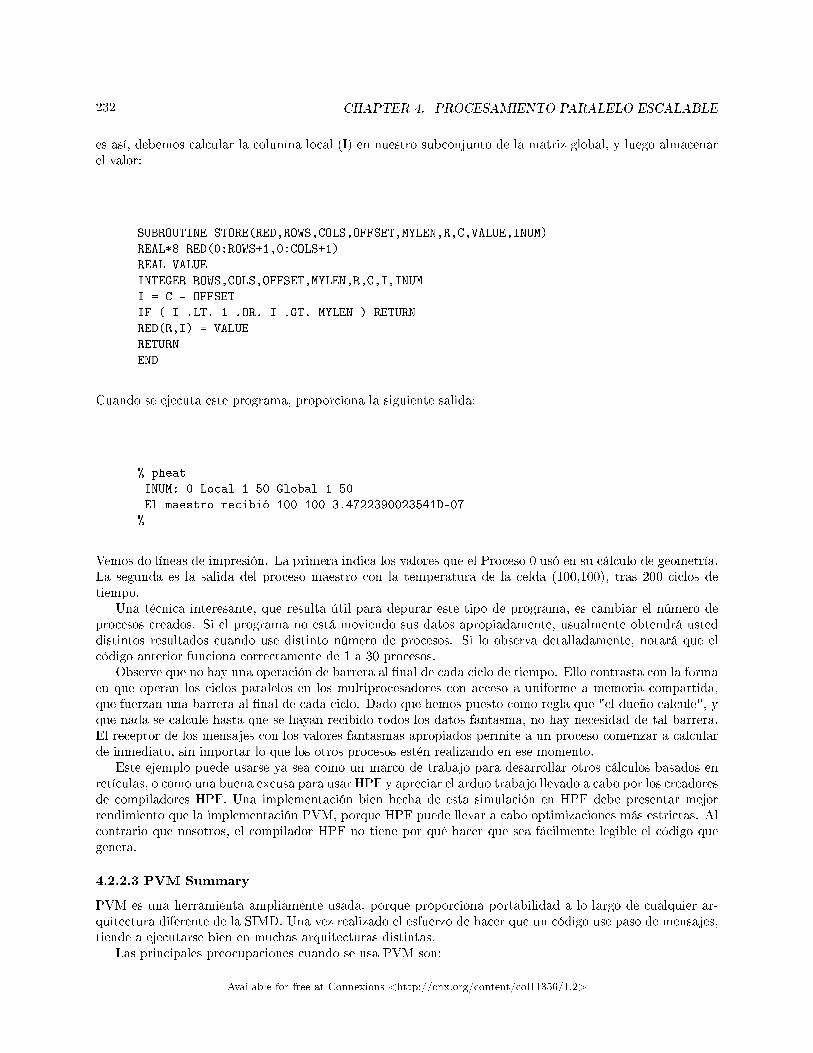
232 CHAPTER 4. PROCESAMIENTO PARALELO ESCALABLE
es así, debemos calcular la columna local (I) en nuestro subconjunto de la matriz global, y luego almacenarel valor:
SUBROUTINE STORE(RED,ROWS,COLS,OFFSET,MYLEN,R,C,VALUE,INUM)
REAL*8 RED(0:ROWS+1,0:COLS+1)
REAL VALUE
INTEGER ROWS,COLS,OFFSET,MYLEN,R,C,I,INUM
I = C - OFFSET
IF ( I .LT. 1 .OR. I .GT. MYLEN ) RETURN
RED(R,I) = VALUE
RETURN
END
Cuando se ejecuta este programa, proporciona la siguiente salida:
% pheat
INUM: 0 Local 1 50 Global 1 50
El maestro recibió 100 100 3.4722390023541D-07
%
Vemos do líneas de impresión. La primera indica los valores que el Proceso 0 usó en su cálculo de geometría.La segunda es la salida del proceso maestro con la temperatura de la celda (100,100), tras 200 ciclos detiempo.
Una técnica interesante, que resulta útil para depurar este tipo de programa, es cambiar el número deprocesos creados. Si el programa no está moviendo sus datos apropiadamente, usualmente obtendrá usteddistintos resultados cuando use distinto número de procesos. Si lo observa detalladamente, notará que elcódigo anterior funciona correctamente de 1 a 30 procesos.
Observe que no hay una operación de barrera al �nal de cada ciclo de tiempo. Ello contrasta con la formaen que operan los ciclos paralelos en los multiprocesadores con acceso a uniforme a memoria compartida,que fuerzan una barrera al �nal de cada ciclo. Dado que hemos puesto como regla que "el dueño calcule", yque nada se calcule hasta que se hayan recibido todos los datos fantasma, no hay necesidad de tal barrera.El receptor de los mensajes con los valores fantasmas apropiados permite a un proceso comenzar a calcularde inmediato, sin importar lo que los otros procesos estén realizando en ese momento.
Este ejemplo puede usarse ya sea como un marco de trabajo para desarrollar otros cálculos basados enretículas, o como una buena excusa para usar HPF y apreciar el arduo trabajo llevado a cabo por los creadoresde compiladores HPF. Una implementación bien hecha de esta simulación en HPF debe presentar mejorrendimiento que la implementación PVM, porque HPF puede llevar a cabo optimizaciones más estrictas. Alcontrario que nosotros, el compilador HPF no tiene por qué hacer que sea fácilmente legible el código quegenera.
4.2.2.3 PVM Summary
PVM es una herramienta ampliamente usada, porque proporciona portabilidad a lo largo de cualquier ar-quitectura diferente de la SIMD. Una vez realizado el esfuerzo de hacer que un código use paso de mensajes,tiende a ejecutarse bien en muchas arquitecturas distintas.
Las principales preocupaciones cuando se usa PVM son:
Available for free at Connexions <http://cnx.org/content/col11356/1.2>
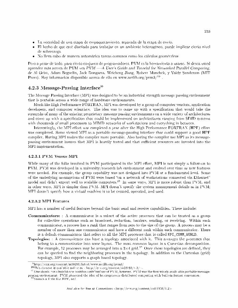
233
• La necesidad de una etapa de empaquetamiento, separada de la etapa de envío.• El hecho de que esté diseñado para trabajar en un ambiente heterogéneo, puede implicar cierto nivel
de sobrecarga• No lleva cabo de manera automática tareas comunes como los cálculos geométricos
Pero a pesar de todo, para cierto conjunto de programadores, PVM es la herramienta a usarse. Si desea ustedaprender más acerca de PVM vea PVM � A User's Guide and Tutorial for Networked Parallel Computing,de Al Geist, Adam Beguelin, Jack Dongarra, Weicheng Jiang, Robert Manchek, y Vaidy Sunderam (MITPress). Hay información disponible acerca de ello en www.netlib.org/pvm3/19 .
4.2.3 Message-Passing Interface20
The Message-Passing Interface (MPI) was designed to be an industrial-strength message-passing environmentthat is portable across a wide range of hardware environments.
Much like High Performance FORTRAN, MPI was developed by a group of computer vendors, applicationdevelopers, and computer scientists. The idea was to come up with a speci�cation that would take thestrengths of many of the existing proprietary message passing environments on a wide variety of architecturesand come up with a speci�cation that could be implemented on architectures ranging from SIMD systemswith thousands of small processors to MIMD networks of workstations and everything in between.
Interestingly, the MPI e�ort was completed a year after the High Performance FORTRAN (HPF) e�ortwas completed. Some viewed MPI as a portable message-passing interface that could support a good HPFcompiler. Having MPI makes the compiler more portable. Also having the compiler use MPI as its message-passing environment insures that MPI is heavily tested and that su�cient resources are invested into theMPI implementation.
4.2.3.1 PVM Versus MPI
While many of the folks involved in PVM participated in the MPI e�ort, MPI is not simply a follow-on toPVM. PVM was developed in a university/research lab environment and evolved over time as new featureswere needed. For example, the group capability was not designed into PVM at a fundamental level. Someof the underlying assumptions of PVM were based �on a network of workstations connected via Ethernet�model and didn't export well to scalable computers.21 In some ways, MPI is more robust than PVM, andin other ways, MPI is simpler than PVM. MPI doesn't specify the system management details as in PVM;MPI doesn't specify how a virtual machine is to be created, operated, and used.
4.2.3.2 MPI Features
MPI has a number of useful features beyond the basic send and receive capabilities. These include:
Communicators: : A communicator is a subset of the active processes that can be treated as a groupfor collective operations such as broadcast, reduction, barriers, sending, or receiving. Within eachcommunicator, a process has a rank that ranges from zero to the size of the group. A process may be amember of more than one communicator and have a di�erent rank within each communicator. Thereis a default communicator that refers to all the MPI processes that is called MPI_COMM_WORLD.
Topologies: : A communicator can have a topology associated with it. This arranges the processes thatbelong to a communicator into some layout. The most common layout is a Cartesian decomposition.For example, 12 processes may be arranged into a 3×4 grid.22 Once these topologies are de�ned, theycan be queried to �nd the neighboring processes in the topology. In addition to the Cartesian (grid)topology, MPI also supports a graph-based topology.
19http://cnx.org/content/m38291/latest/www.netlib.org/pvm3/20This content is available online at <http://cnx.org/content/m33783/1.3/>.21One should not diminish the positive contributions of PVM, however. PVM was the �rst widely avail- able portable message-
passing environment. PVM pioneered the idea of heterogeneous distributed computing with built-in format conversion.22Sounds a little like HPF, no?
Available for free at Connexions <http://cnx.org/content/col11356/1.2>
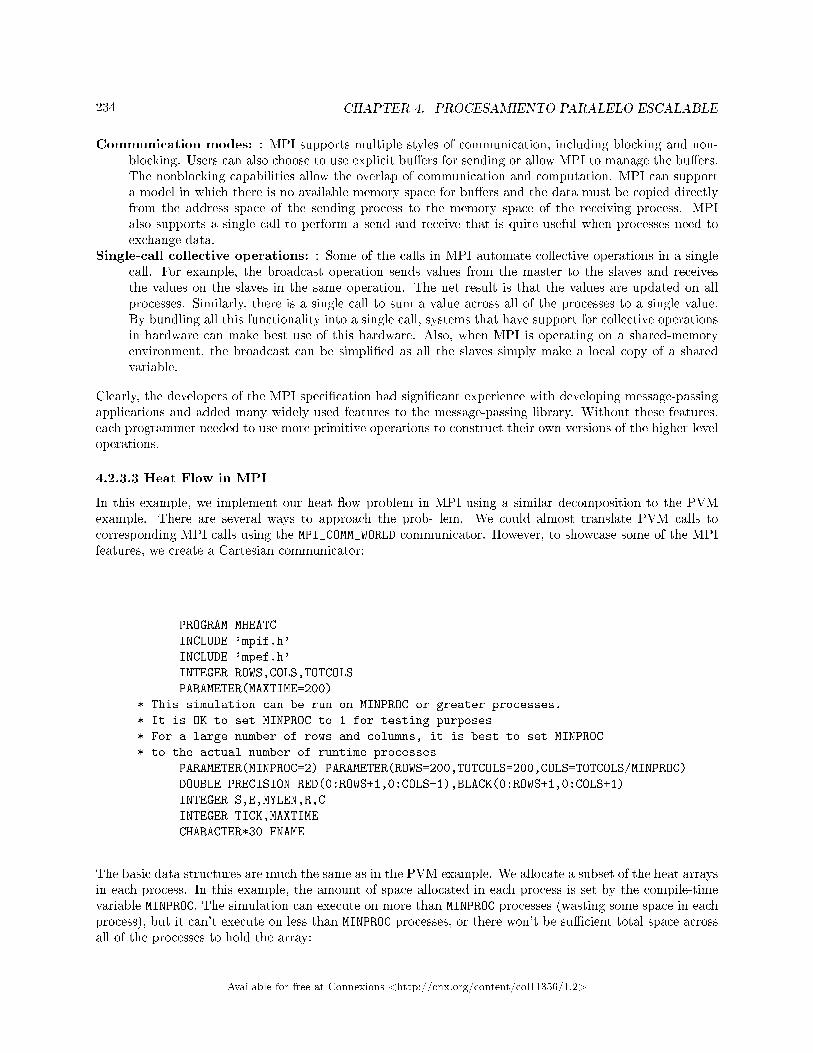
234 CHAPTER 4. PROCESAMIENTO PARALELO ESCALABLE
Communication modes: : MPI supports multiple styles of communication, including blocking and non-blocking. Users can also choose to use explicit bu�ers for sending or allow MPI to manage the bu�ers.The nonblocking capabilities allow the overlap of communication and computation. MPI can supporta model in which there is no available memory space for bu�ers and the data must be copied directlyfrom the address space of the sending process to the memory space of the receiving process. MPIalso supports a single call to perform a send and receive that is quite useful when processes need toexchange data.
Single-call collective operations: : Some of the calls in MPI automate collective operations in a singlecall. For example, the broadcast operation sends values from the master to the slaves and receivesthe values on the slaves in the same operation. The net result is that the values are updated on allprocesses. Similarly, there is a single call to sum a value across all of the processes to a single value.By bundling all this functionality into a single call, systems that have support for collective operationsin hardware can make best use of this hardware. Also, when MPI is operating on a shared-memoryenvironment, the broadcast can be simpli�ed as all the slaves simply make a local copy of a sharedvariable.
Clearly, the developers of the MPI speci�cation had signi�cant experience with developing message-passingapplications and added many widely used features to the message-passing library. Without these features,each programmer needed to use more primitive operations to construct their own versions of the higher-leveloperations.
4.2.3.3 Heat Flow in MPI
In this example, we implement our heat �ow problem in MPI using a similar decomposition to the PVMexample. There are several ways to approach the prob- lem. We could almost translate PVM calls tocorresponding MPI calls using the MPI_COMM_WORLD communicator. However, to showcase some of the MPIfeatures, we create a Cartesian communicator:
PROGRAM MHEATC
INCLUDE 'mpif.h'
INCLUDE 'mpef.h'
INTEGER ROWS,COLS,TOTCOLS
PARAMETER(MAXTIME=200)
* This simulation can be run on MINPROC or greater processes.
* It is OK to set MINPROC to 1 for testing purposes
* For a large number of rows and columns, it is best to set MINPROC
* to the actual number of runtime processes
PARAMETER(MINPROC=2) PARAMETER(ROWS=200,TOTCOLS=200,COLS=TOTCOLS/MINPROC)
DOUBLE PRECISION RED(0:ROWS+1,0:COLS+1),BLACK(0:ROWS+1,0:COLS+1)
INTEGER S,E,MYLEN,R,C
INTEGER TICK,MAXTIME
CHARACTER*30 FNAME
The basic data structures are much the same as in the PVM example. We allocate a subset of the heat arraysin each process. In this example, the amount of space allocated in each process is set by the compile-timevariable MINPROC. The simulation can execute on more than MINPROC processes (wasting some space in eachprocess), but it can't execute on less than MINPROC processes, or there won't be su�cient total space acrossall of the processes to hold the array:
Available for free at Connexions <http://cnx.org/content/col11356/1.2>
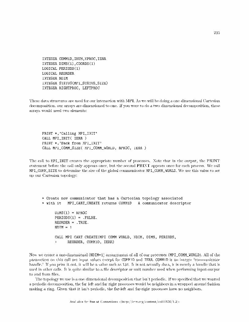
235
INTEGER COMM1D,INUM,NPROC,IERR
INTEGER DIMS(1),COORDS(1)
LOGICAL PERIODS(1)
LOGICAL REORDER
INTEGER NDIM
INTEGER STATUS(MPI_STATUS_SIZE)
INTEGER RIGHTPROC, LEFTPROC
These data structures are used for our interaction with MPI. As we will be doing a one-dimensional Cartesiandecomposition, our arrays are dimensioned to one. If you were to do a two-dimensional decomposition, thesearrays would need two elements:
PRINT *,'Calling MPI_INIT'
CALL MPI_INIT( IERR )
PRINT *,'Back from MPI_INIT'
CALL MPI_COMM_SIZE( MPI_COMM_WORLD, NPROC, IERR )
The call to MPI_INIT creates the appropriate number of processes. Note that in the output, the PRINTstatement before the call only appears once, but the second PRINT appears once for each process. We callMPI_COMM_SIZE to determine the size of the global communicator MPI_COMM_WORLD. We use this value to setup our Cartesian topology:
* Create new communicator that has a Cartesian topology associated
* with it - MPI_CART_CREATE returns COMM1D - A communicator descriptor
DIMS(1) = NPROC
PERIODS(1) = .FALSE.
REORDER = .TRUE.
NDIM = 1
CALL MPI_CART_CREATE(MPI_COMM_WORLD, NDIM, DIMS, PERIODS,
+ REORDER, COMM1D, IERR)
Now we create a one-dimensional (NDIM=1) arrangement of all of our processes (MPI_COMM_WORLD). All of theparameters on this call are input values except for COMM1D and IERR. COMM1D is an integer �communicatorhandle.� If you print it out, it will be a value such as 134. It is not actually data, it is merely a handle that isused in other calls. It is quite similar to a �le descriptor or unit number used when performing input-outputto and from �les.
The topology we use is a one-dimensional decomposition that isn't periodic. If we speci�ed that we wanteda periodic decomposition, the far-left and far-right processes would be neighbors in a wrapped-around fashionmaking a ring. Given that it isn't periodic, the far-left and far-right processes have no neighbors.
Available for free at Connexions <http://cnx.org/content/col11356/1.2>

236 CHAPTER 4. PROCESAMIENTO PARALELO ESCALABLE
In our PVM example above, we declared that Process 0 was the far-right process, Process NPROC-1 wasthe far-left process, and the other processes were arranged linearly between those two. If we set REORDERto .FALSE., MPI also chooses this arrangement. However, if we set REORDER to .TRUE., MPI may choose toarrange the processes in some other fashion to achieve better performance, assuming that you are commu-nicating with close neighbors.
Once the communicator is set up, we use it in all of our communication operations:
* Get my rank in the new communicator
CALL MPI_COMM_RANK( COMM1D, INUM, IERR)
Within each communicator, each process has a rank from zero to the size of the communicator minus 1. TheMPI_COMM_RANK tells each process its rank within the communicator. A process may have a di�erent rank inthe COMM1D communicator than in the MPI_COMM_WORLD communicator because of some reordering.
Given a Cartesian topology communicator,23 we can extract information from the communicator usingthe MPI_CART_GET routine:
* Given a communicator handle COMM1D, get the topology, and my position
* in the topology
CALL MPI_CART_GET(COMM1D, NDIM, DIMS, PERIODS, COORDS, IERR)
In this call, all of the parameters are output values rather than input values as in the MPI_CART_CREATE
call. The COORDS variable tells us our coordinates within the communicator. This is not so useful in ourone-dimensional example, but in a two-dimensional process decomposition, it would tell our current positionin that two-dimensional grid:
* Returns the left and right neighbors 1 unit away in the zeroth dimension
* of our Cartesian map - since we are not periodic, our neighbors may
* not always exist - MPI_CART_SHIFT handles this for us
CALL MPI_CART_SHIFT(COMM1D, 0, 1, LEFTPROC, RIGHTPROC, IERR)
CALL MPE_DECOMP1D(TOTCOLS, NPROC, INUM, S, E)
MYLEN = ( E - S ) + 1
IF ( MYLEN.GT.COLS ) THEN
PRINT *,'Not enough space, need',MYLEN,' have ',COLS
PRINT *,TOTCOLS,NPROC,INUM,S,E
STOP
ENDIF
PRINT *,INUM,NPROC,COORDS(1),LEFTPROC,RIGHTPROC, S, E
23Remember, each communicator may have a topology associated with it. A topology can be grid, graph, or none. Interest-ingly, the MPI_COMM_WORLD communicator has no topology associated with it.
Available for free at Connexions <http://cnx.org/content/col11356/1.2>
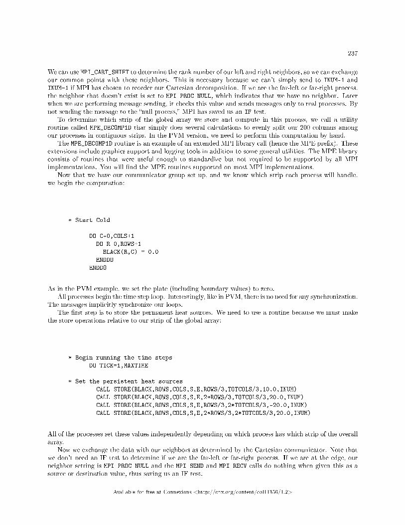
237
We can use MPI_CART_SHIFT to determine the rank number of our left and right neighbors, so we can exchangeour common points with these neighbors. This is necessary because we can't simply send to INUM-1 andINUM+1 if MPI has chosen to reorder our Cartesian decomposition. If we are the far-left or far-right process,the neighbor that doesn't exist is set to MPI_PROC_NULL, which indicates that we have no neighbor. Laterwhen we are performing message sending, it checks this value and sends messages only to real processes. Bynot sending the message to the �null process,� MPI has saved us an IF test.
To determine which strip of the global array we store and compute in this process, we call a utilityroutine called MPE_DECOMP1D that simply does several calculations to evenly split our 200 columns amongour processes in contiguous strips. In the PVM version, we need to perform this computation by hand.
The MPE_DECOMP1D routine is an example of an extended MPI library call (hence the MPE pre�x). Theseextensions include graphics support and logging tools in addition to some general utilities. The MPE libraryconsists of routines that were useful enough to standardize but not required to be supported by all MPIimplementations. You will �nd the MPE routines supported on most MPI implementations.
Now that we have our communicator group set up, and we know which strip each process will handle,we begin the computation:
* Start Cold
DO C=0,COLS+1
DO R=0,ROWS+1
BLACK(R,C) = 0.0
ENDDO
ENDDO
As in the PVM example, we set the plate (including boundary values) to zero.All processes begin the time step loop. Interestingly, like in PVM, there is no need for any synchronization.
The messages implicitly synchronize our loops.The �rst step is to store the permanent heat sources. We need to use a routine because we must make
the store operations relative to our strip of the global array:
* Begin running the time steps
DO TICK=1,MAXTIME
* Set the persistent heat sources
CALL STORE(BLACK,ROWS,COLS,S,E,ROWS/3,TOTCOLS/3,10.0,INUM)
CALL STORE(BLACK,ROWS,COLS,S,E,2*ROWS/3,TOTCOLS/3,20.0,INUM)
CALL STORE(BLACK,ROWS,COLS,S,E,ROWS/3,2*TOTCOLS/3,-20.0,INUM)
CALL STORE(BLACK,ROWS,COLS,S,E,2*ROWS/3,2*TOTCOLS/3,20.0,INUM)
All of the processes set these values independently depending on which process has which strip of the overallarray.
Now we exchange the data with our neighbors as determined by the Cartesian communicator. Note thatwe don't need an IF test to determine if we are the far-left or far-right process. If we are at the edge, ourneighbor setting is MPI_PROC_NULL and the MPI_SEND and MPI_RECV calls do nothing when given this as asource or destination value, thus saving us an IF test.
Available for free at Connexions <http://cnx.org/content/col11356/1.2>
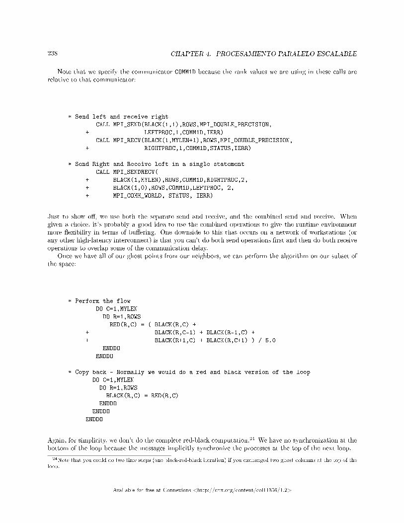
238 CHAPTER 4. PROCESAMIENTO PARALELO ESCALABLE
Note that we specify the communicator COMM1D because the rank values we are using in these calls arerelative to that communicator:
* Send left and receive right
CALL MPI_SEND(BLACK(1,1),ROWS,MPI_DOUBLE_PRECISION,
+ LEFTPROC,1,COMM1D,IERR)
CALL MPI_RECV(BLACK(1,MYLEN+1),ROWS,MPI_DOUBLE_PRECISION,
+ RIGHTPROC,1,COMM1D,STATUS,IERR)
* Send Right and Receive left in a single statement
CALL MPI_SENDRECV(
+ BLACK(1,MYLEN),ROWS,COMM1D,RIGHTPROC,2,
+ BLACK(1,0),ROWS,COMM1D,LEFTPROC, 2,
+ MPI_COMM_WORLD, STATUS, IERR)
Just to show o�, we use both the separate send and receive, and the combined send and receive. Whengiven a choice, it's probably a good idea to use the combined operations to give the runtime environmentmore �exibility in terms of bu�ering. One downside to this that occurs on a network of workstations (orany other high-latency interconnect) is that you can't do both send operations �rst and then do both receiveoperations to overlap some of the communication delay.
Once we have all of our ghost points from our neighbors, we can perform the algorithm on our subset ofthe space:
* Perform the flow
DO C=1,MYLEN
DO R=1,ROWS
RED(R,C) = ( BLACK(R,C) +
+ BLACK(R,C-1) + BLACK(R-1,C) +
+ BLACK(R+1,C) + BLACK(R,C+1) ) / 5.0
ENDDO
ENDDO
* Copy back - Normally we would do a red and black version of the loop
DO C=1,MYLEN
DO R=1,ROWS
BLACK(R,C) = RED(R,C)
ENDDO
ENDDO
ENDDO
Again, for simplicity, we don't do the complete red-black computation.24 We have no synchronization at thebottom of the loop because the messages implicitly synchronize the processes at the top of the next loop.
24Note that you could do two time steps (one black-red-black iteration) if you exchanged two ghost columns at the top of theloop.
Available for free at Connexions <http://cnx.org/content/col11356/1.2>

239
Again, we dump out the data for veri�cation. As in the PVM example, one good test of basic correctnessis to make sure you get exactly the same results for varying numbers of processes:
* Dump out data for verification
IF ( ROWS .LE. 20 ) THEN
FNAME = '/tmp/mheatcout.' // CHAR(ICHAR('0')+INUM)
OPEN(UNIT=9,NAME=FNAME,FORM='formatted')
DO C=1,MYLEN
WRITE(9,100)(BLACK(R,C),R=1,ROWS)
100 FORMAT(20F12.6)
ENDDO
CLOSE(UNIT=9)
ENDIF
To terminate the program, we call MPI_FINALIZE:
* Lets all go together
CALL MPI_FINALIZE(IERR)
END
As in the PVM example, we need a routine to store a value into the proper strip of the global array. Thisroutine simply checks to see if a particular global element is in this process and if so, computes the properlocation within its strip for the value. If the global element is not in this process, this routine simply returnsdoing nothing:
SUBROUTINE STORE(RED,ROWS,COLS,S,E,R,C,VALUE,INUM)
REAL*8 RED(0:ROWS+1,0:COLS+1)
REAL VALUE
INTEGER ROWS,COLS,S,E,R,C,I,INUM
IF ( C .LT. S .OR. C .GT. E ) RETURN
I = ( C - S ) + 1
* PRINT *,'STORE, INUM,R,C,S,E,R,I',INUM,R,C,S,E,R,I,VALUE RED(R,I) = VALUE
RETURN
END
When this program is executed, it has the following output:
% mpif77 -c mheatc.f mheatc.f:
MAIN mheatc:
Available for free at Connexions <http://cnx.org/content/col11356/1.2>
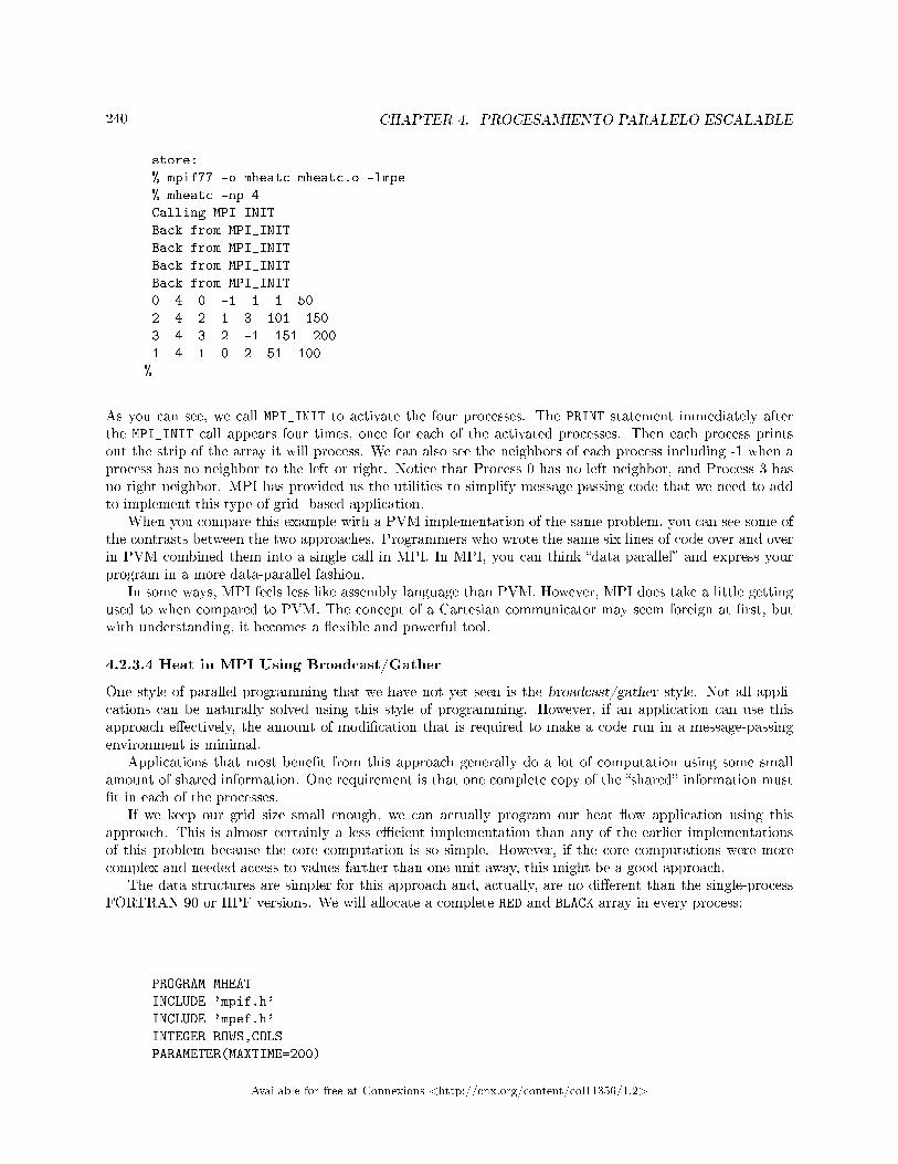
240 CHAPTER 4. PROCESAMIENTO PARALELO ESCALABLE
store:
% mpif77 -o mheatc mheatc.o -lmpe
% mheatc -np 4
Calling MPI_INIT
Back from MPI_INIT
Back from MPI_INIT
Back from MPI_INIT
Back from MPI_INIT
0 4 0 -1 1 1 50
2 4 2 1 3 101 150
3 4 3 2 -1 151 200
1 4 1 0 2 51 100
%
As you can see, we call MPI_INIT to activate the four processes. The PRINT statement immediately afterthe MPI_INIT call appears four times, once for each of the activated processes. Then each process printsout the strip of the array it will process. We can also see the neighbors of each process including -1 when aprocess has no neighbor to the left or right. Notice that Process 0 has no left neighbor, and Process 3 hasno right neighbor. MPI has provided us the utilities to simplify message-passing code that we need to addto implement this type of grid- based application.
When you compare this example with a PVM implementation of the same problem, you can see some ofthe contrasts between the two approaches. Programmers who wrote the same six lines of code over and overin PVM combined them into a single call in MPI. In MPI, you can think �data parallel� and express yourprogram in a more data-parallel fashion.
In some ways, MPI feels less like assembly language than PVM. However, MPI does take a little gettingused to when compared to PVM. The concept of a Cartesian communicator may seem foreign at �rst, butwith understanding, it becomes a �exible and powerful tool.
4.2.3.4 Heat in MPI Using Broadcast/Gather
One style of parallel programming that we have not yet seen is the broadcast/gather style. Not all appli-cations can be naturally solved using this style of programming. However, if an application can use thisapproach e�ectively, the amount of modi�cation that is required to make a code run in a message-passingenvironment is minimal.
Applications that most bene�t from this approach generally do a lot of computation using some smallamount of shared information. One requirement is that one complete copy of the �shared� information must�t in each of the processes.
If we keep our grid size small enough, we can actually program our heat �ow application using thisapproach. This is almost certainly a less e�cient implementation than any of the earlier implementationsof this problem because the core computation is so simple. However, if the core computations were morecomplex and needed access to values farther than one unit away, this might be a good approach.
The data structures are simpler for this approach and, actually, are no di�erent than the single-processFORTRAN 90 or HPF versions. We will allocate a complete RED and BLACK array in every process:
PROGRAM MHEAT
INCLUDE 'mpif.h'
INCLUDE 'mpef.h'
INTEGER ROWS,COLS
PARAMETER(MAXTIME=200)
Available for free at Connexions <http://cnx.org/content/col11356/1.2>
241
PARAMETER(ROWS=200,COLS=200)
DOUBLE PRECISION RED(0:ROWS+1,0:COLS+1),BLACK(0:ROWS+1,0:COLS+1)
We need fewer variables for the MPI calls because we aren't creating a communicator. We simply use thedefault communicator MPI_COMM_WORLD. We start up our processes, and �nd the size and rank of our processgroup:
INTEGER INUM,NPROC,IERR,SRC,DEST,TAG
INTEGER S,E,LS,LE,MYLEN
INTEGER STATUS(MPI_STATUS_SIZE)
INTEGER I,R,C
INTEGER TICK,MAXTIME
CHARACTER*30 FNAME
PRINT *,'Calling MPI_INIT'
CALL MPI_INIT( IERR )
CALL MPI_COMM_SIZE( MPI_COMM_WORLD, NPROC, IERR )
CALL MPI_COMM_RANK( MPI_COMM_WORLD, INUM, IERR)
CALL MPE_DECOMP1D(COLS, NPROC, INUM, S, E, IERR)
PRINT *,'My Share ', INUM, NPROC, S, E
Since we are broadcasting initial values to all of the processes, we only have to set things up on the masterprocess:
* Start Cold
IF ( INUM.EQ.0 ) THEN
DO C=0,COLS+1
DO R=0,ROWS+1
BLACK(R,C) = 0.0
ENDDO
ENDDO
ENDIF
As we run the time steps (again with no synchronization), we set the persistent heat sources directly. Sincethe shape of the data structure is the same in the master and all other processes, we can use the real arraycoordinates rather than mapping them as with the previous examples. We could skip the persistent settingson the nonmaster processes, but it doesn't hurt to do it on all processes:
* Begin running the time steps
DO TICK=1,MAXTIME
Available for free at Connexions <http://cnx.org/content/col11356/1.2>
242 CHAPTER 4. PROCESAMIENTO PARALELO ESCALABLE
* Set the heat sources
BLACK(ROWS/3, COLS/3)= 10.0
BLACK(2*ROWS/3, COLS/3) = 20.0
BLACK(ROWS/3, 2*COLS/3) = -20.0
BLACK(2*ROWS/3, 2*COLS/3) = 20.0
Now we broadcast the entire array from process rank zero to all of the other processes in the MPI_COMM_WORLDcommunicator. Note that this call does the sending on rank zero process and receiving on the other processes.The net result of this call is that all the processes have the values formerly in the master process in a singlecall:
* Broadcast the array
CALL MPI_BCAST(BLACK,(ROWS+2)*(COLS+2),MPI_DOUBLE_PRECISION,
+ 0,MPI_COMM_WORLD,IERR)
Now we perform the subset computation on each process. Note that we are using global coordinates becausethe array has the same shape on each of the processes. All we need to do is make sure we set up our particularstrip of columns according to S and E:
* Perform the flow on our subset
DO C=S,E
DO R=1,ROWS
RED(R,C) = ( BLACK(R,C) +
+ BLACK(R,C-1) + BLACK(R-1,C) +
+ BLACK(R+1,C) + BLACK(R,C+1) ) / 5.0
ENDDO
ENDDO
Now we need to gather the appropriate strips from the processes into the appropriate strip in the masterarray for rebroadcast in the next time step. We could change the loop in the master to receive the messagesin any order and check the STATUS variable to see which strip it received:
* Gather back up into the BLACK array in master (INUM = 0)
IF ( INUM .EQ. 0 ) THEN
DO C=S,E
DO R=1,ROWS
BLACK(R,C) = RED(R,C)
ENDDO
ENDDO
DO I=1,NPROC-1
CALL MPE_DECOMP1D(COLS, NPROC, I, LS, LE, IERR)
Available for free at Connexions <http://cnx.org/content/col11356/1.2>
243
MYLEN = ( LE - LS ) + 1
SRC = I TAG = 0
CALL MPI_RECV(BLACK(0,LS),MYLEN*(ROWS+2),
+ MPI_DOUBLE_PRECISION, SRC, TAG,
+ MPI_COMM_WORLD, STATUS, IERR)
* Print *,'Recv',I,MYLEN
ENDDO
ELSE
MYLEN = ( E - S ) + 1
DEST = 0
TAG = 0
CALL MPI_SEND(RED(0,S),MYLEN*(ROWS+2),MPI_DOUBLE_PRECISION,
+ DEST, TAG, MPI_COMM_WORLD, IERR)
Print *,'Send',INUM,MYLEN
ENDIF
ENDDO
We use MPE_DECOMP1D to determine which strip we're receiving from each process.In some applications, the value that must be gathered is a sum or another single value. To accomplish
this, you can use one of the MPI reduction routines that coalesce a set of distributed values into a singlevalue using a single call.
Again at the end, we dump out the data for testing. However, since it has all been gathered back ontothe master process, we only need to dump it on one process:
* Dump out data for verification
IF ( INUM .EQ.0 .AND. ROWS .LE. 20 ) THEN
FNAME = '/tmp/mheatout'
OPEN(UNIT=9,NAME=FNAME,FORM='formatted')
DO C=1,COLS
WRITE(9,100)(BLACK(R,C),R=1,ROWS)
100 FORMAT(20F12.6)
ENDDO
CLOSE(UNIT=9)
ENDIF
CALL MPI_FINALIZE(IERR)
END
When this program executes with four processes, it produces the following output:
% mpif77 -c mheat.f
mheat.f:
MAIN mheat:
% mpif77 -o mheat mheat.o -lmpe
% mheat -np 4
Available for free at Connexions <http://cnx.org/content/col11356/1.2>

244 CHAPTER 4. PROCESAMIENTO PARALELO ESCALABLE
Calling MPI_INIT
My Share 1 4 51 100
My Share 0 4 1 50
My Share 3 4 151 200
My Share 2 4 101 150
%
The ranks of the processes and the subsets of the computations for each process are shown in the output.So that is a somewhat contrived example of the broadcast/gather approach to parallelizing an applica-
tion. If the data structures are the right size and the amount of computation relative to communication isappropriate, this can be a very e�ective approach that may require the smallest number of code modi�cationscompared to a single-processor version of the code.
4.2.3.5 MPI Summary
Whether you chose PVM or MPI depends on which library the vendor of your system prefers. SometimesMPI is the better choice because it contains the newest features, such as support for hardware-supportedmulticast or broadcast, that can signi�cantly improve the overall performance of a scatter-gather application.
A good text on MPI is Using MPI � Portable Parallel Programmingwith the Message-Passing Interface,by William Gropp, Ewing Lusk, and Anthony Skjellum (MIT Press). You may also want to retrieve andprint the MPI speci�cation from http://www.netlib.org/mpi/25 .
4.2.4 Closing Notes26
In this chapter we have looked at the �assembly language� of parallel programming. While it can seemdaunting to rethink your application, there are often some simple changes you can make to port your codeto message passing. Depending on the application, a master-slave, broadcast-gather, or decomposed dataapproach might be most appropriate.
It's important to realize that some applications just don't decompose into message passing very well.You may be working with just such an application. Once you have some experience with message passing,it becomes easier to identify the critical points where data must be communicated between processes.
While HPF, PVM, and MPI are all mature and popular technologies, it's not clear whether any of thesetechnologies will be the long-term solution that we will use 10 years from now. One possibility is that wewill use FORTRAN 90 (or FORTRAN 95) without any data layout directives or that the directives will beoptional. Another interesting possibility is simply to keep using FORTRAN 77. As scalable, cache-coherent,non-uniform memory systems become more popular, they will evolve their own data allocation primitives.For example, the HP/Exemplar supports the following data storage attributes: shared, node-private, andthread-private. As dynamic data structures are allocated, they can be placed in any one of these classes.Node-private memory is shared across all the threads on a single node but not shared beyond those threads.Perhaps we will only have to declare the storage class of the data but not the data layout for these newmachines.
PVM and MPI still need the capability of supporting a fault-tolerant style of computing that allows anapplication to complete as resources fail or otherwise become available. The amount of compute power thatwill be available to applications that can tolerate some unreliability in the resources will be very large. Therehave been a number of moderately successful attempts in this area such as Condor, but none have reallycaught on in the mainstream.
To run the most powerful computers in the world at their absolute maximum performance levels, theneed to be portable is somewhat reduced. Making your particular application go ever faster and scale toever higher numbers of processors is a fascinating activity. May the FLOPS be with you!
25http://www.netlib.org/mpi/26This content is available online at <http://cnx.org/content/m33784/1.3/>.
Available for free at Connexions <http://cnx.org/content/col11356/1.2>
Chapter 5
Apéndices
5.1 Appendix C: High Performance Microprocessors
5.1.1 Introduction1
5.1.1.1 High Performance Microprocessors
It has been said that history is rewritten by the victors. It is clear that high performance RISC-basedmicroprocessors are de�ning the current history of high performance computing. We begin our study with thebasic building blocks of modern high performance computing: the high performance RISC microprocessors.
A complex instruction set computer (CISC) instruction set is made up of powerful primitives, close infunctionality to the primitives of high-level languages like C or FORTRAN. It captures the sense of �don'tdo in software what you can do in hardware.� RISC, on the other hand, emphasizes low-level primitives, farbelow the complexity of a high-level language. You can compute anything you want using either approach,though it will probably take more machine instructions if you're using RISC. The important di�erence isthat with RISC you can trade instruction-set complexity for speed.
To be fair, RISC isn't really all that new. There were some important early machines that pioneeredRISC philosophies, such as the CDC 6600 (1964) and the IBM 801 project (1975). It was in the mid-1980s,however, that RISC machines �rst posed a direct challenge to the CISC installed base. Heated debate brokeout � RISC versus CISC � and even lingers today, though it is clear that the RISC2 approach is in greatestfavor; late-generation CISC machines are looking more RISC-like, and some very old families of CISC, suchas the DEC VAX, are being retired.
This chapter is about CISC and RISC instruction set architectures and the di�erences between them.We also describe newer processors that can execute more than one instruction at a time and can executeinstructions out of order.
5.1.2 Why CISC?3
You might ask, �If RISC is faster, why did people bother with CISC designs in the �rst place?� The shortanswer is that in the beginning, CISC was the right way to go; RISC wasn't always both feasible anda�ordable. Every kind of design incorporates trade-o�s, and over time, the best systems will make themdi�erently. In the past, the design variables favored CISC.
1This content is available online at <http://cnx.org/content/m33671/1.3/>.2One of the most interesting remaining topics is the de�nition of �RISC.� Don't be fooled into thinking there is one de�nition
of RISC. The best I have heard so far is from John Mashey: �RISC is a label most commonly used for a set of instruction setarchitecture characteristics chosen to ease the use of aggressive implementation techniques found in high performance processors(regardless of RISC, CISC, or irrelevant).�
3This content is available online at <http://cnx.org/content/m33672/1.3/>.
Available for free at Connexions <http://cnx.org/content/col11356/1.2>
245
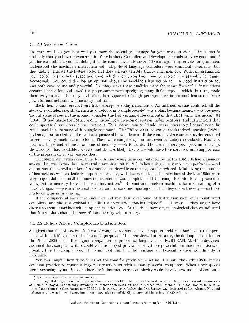
246 CHAPTER 5. APÉNDICES
5.1.2.1 Space and Time
To start, we'll ask you how well you know the assembly language for your work- station. The answer isprobably that you haven't even seen it. Why bother? Compilers and development tools are very good, and ifyou have a problem, you can debug it at the source level. However, 30 years ago, �respectable� programmersunderstood the machine's instruction set. High-level language compilers were commonly available, butthey didn't generate the fastest code, and they weren't terribly thrifty with memory. When programming,you needed to save both space and time, which meant you knew how to program in assembly language.Accordingly, you could develop an opinion about the machine's instruction set. A good instruction setwas both easy to use and powerful. In many ways these qualities were the same: �powerful� instructionsaccomplished a lot, and saved the programmer from specifying many little steps � which, in turn, madethem easy to use. But they had other, less apparent (though perhaps more important) features as well:powerful instructions saved memory and time.
Back then, computers had very little storage by today's standards. An instruction that could roll all thesteps of a complex operation, such as a do-loop, into single opcode4 was a plus, because memory was precious.To put some stakes in the ground, consider the last vacuum-tube computer that IBM built, the model 704(1956). It had hardware �oating-point, including a division operation, index registers, and instructions thatcould operate directly on memory locations. For instance, you could add two numbers together and store theresult back into memory with a single command. The Philco 2000, an early transistorized machine (1959),had an operation that could repeat a sequence of instructions until the contents of a counter was decrementedto zero � very much like a do-loop. These were complex operations, even by today's standards. However,both machines had a limited amount of memory � 32-K words. The less memory your program took up,the more you had available for data, and the less likely that you would have to resort to overlaying portionsof the program on top of one another.
Complex instructions saved time, too. Almost every large computer following the IBM 704 had a memorysystem that was slower than its central processing unit (CPU). When a single instruction can perform severaloperations, the overall number of instructions retrieved from memory can be reduced. Minimizing the numberof instructions was particularly important because, with few exceptions, the machines of the late 1950s werevery sequential; not until the current instruction was completed did the computer initiate the process ofgoing out to memory to get the next instruction.5 By contrast, modern machines form something of abucket brigade � passing instructions in from memory and �guring out what they do on the way � so thereare fewer gaps in processing.
If the designers of early machines had had very fast and abundant instruction memory, sophisticatedcompilers, and the wherewithal to build the instruction �bucket brigade� � cheaply � they might havechosen to create machines with simple instruction sets. At the time, however, technological choices indicatedthat instructions should be powerful and thrifty with memory.
5.1.2.2 Beliefs About Complex Instruction Sets
So, given that the lot was cast in favor of complex instruction sets, computer architects had license to experi-ment with matching them to the intended purposes of the machines. For instance, the do-loop instruction onthe Philco 2000 looked like a good companion for procedural languages like FORTRAN. Machine designersassumed that compiler writers could generate object programs using these powerful machine instructions, orpossibly that the compiler could be eliminated, and that the machine could execute source code directly inhardware.
You can imagine how these ideas set the tone for product marketing. Up until the early 1980s, it wascommon practice to equate a bigger instruction set with a more powerful computer. When clock speedswere increasing by multiples, no increase in instruction set complexity could fetter a new model of computer
4Opcode = operation code = instruction.5In 1955, IBM began constructing a machine known as Stretch. It was the �rst computer to process several instructions
at a time in stages, so that they streamed in, rather than being fetched in a piece- meal fashion. The goal was to make it 25times faster than the then brand-new IBM 704. It was six years before the �rst Stretch was delivered to Los Alamos NationalLaboratory. It was indeed faster, but it was expensive to build. Eight were sold for a loss of $20 million.
Available for free at Connexions <http://cnx.org/content/col11356/1.2>
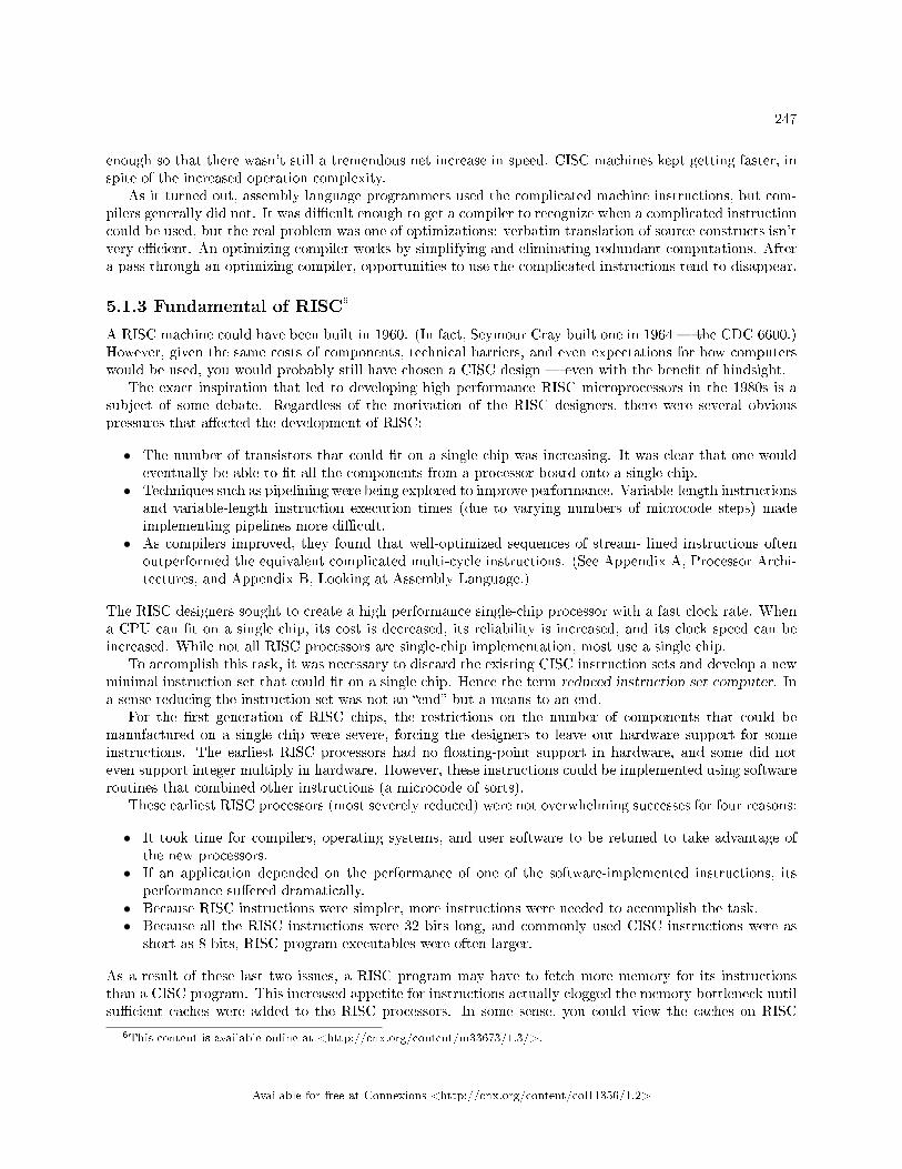
247
enough so that there wasn't still a tremendous net increase in speed. CISC machines kept getting faster, inspite of the increased operation complexity.
As it turned out, assembly language programmers used the complicated machine instructions, but com-pilers generally did not. It was di�cult enough to get a compiler to recognize when a complicated instructioncould be used, but the real problem was one of optimizations: verbatim translation of source constructs isn'tvery e�cient. An optimizing compiler works by simplifying and eliminating redundant computations. Aftera pass through an optimizing compiler, opportunities to use the complicated instructions tend to disappear.
5.1.3 Fundamental of RISC6
A RISC machine could have been built in 1960. (In fact, Seymour Cray built one in 1964 � the CDC 6600.)However, given the same costs of components, technical barriers, and even expectations for how computerswould be used, you would probably still have chosen a CISC design � even with the bene�t of hindsight.
The exact inspiration that led to developing high performance RISC microprocessors in the 1980s is asubject of some debate. Regardless of the motivation of the RISC designers, there were several obviouspressures that a�ected the development of RISC:
• The number of transistors that could �t on a single chip was increasing. It was clear that one wouldeventually be able to �t all the components from a processor board onto a single chip.
• Techniques such as pipelining were being explored to improve performance. Variable-length instructionsand variable-length instruction execution times (due to varying numbers of microcode steps) madeimplementing pipelines more di�cult.
• As compilers improved, they found that well-optimized sequences of stream- lined instructions oftenoutperformed the equivalent complicated multi-cycle instructions. (See Appendix A, Processor Archi-tectures, and Appendix B, Looking at Assembly Language.)
The RISC designers sought to create a high performance single-chip processor with a fast clock rate. Whena CPU can �t on a single chip, its cost is decreased, its reliability is increased, and its clock speed can beincreased. While not all RISC processors are single-chip implementation, most use a single chip.
To accomplish this task, it was necessary to discard the existing CISC instruction sets and develop a newminimal instruction set that could �t on a single chip. Hence the term reduced instruction set computer. Ina sense reducing the instruction set was not an �end� but a means to an end.
For the �rst generation of RISC chips, the restrictions on the number of components that could bemanufactured on a single chip were severe, forcing the designers to leave out hardware support for someinstructions. The earliest RISC processors had no �oating-point support in hardware, and some did noteven support integer multiply in hardware. However, these instructions could be implemented using softwareroutines that combined other instructions (a microcode of sorts).
These earliest RISC processors (most severely reduced) were not overwhelming successes for four reasons:
• It took time for compilers, operating systems, and user software to be retuned to take advantage ofthe new processors.
• If an application depended on the performance of one of the software-implemented instructions, itsperformance su�ered dramatically.
• Because RISC instructions were simpler, more instructions were needed to accomplish the task.• Because all the RISC instructions were 32 bits long, and commonly used CISC instructions were as
short as 8 bits, RISC program executables were often larger.
As a result of these last two issues, a RISC program may have to fetch more memory for its instructionsthan a CISC program. This increased appetite for instructions actually clogged the memory bottleneck untilsu�cient caches were added to the RISC processors. In some sense, you could view the caches on RISC
6This content is available online at <http://cnx.org/content/m33673/1.3/>.
Available for free at Connexions <http://cnx.org/content/col11356/1.2>

248 CHAPTER 5. APÉNDICES
processors as the microcode store in a CISC processor. Both reduced the overall appetite for instructionsthat were loaded from memory.
While the RISC processor designers worked out these issues and the manufacturing capability improved,there was a battle between the existing (now called CISC) processors and the new RISC (not yet successful)processors. The CISC processor designers had mature designs and well-tuned popular software. They alsokept adding performance tricks to their systems. By the time Motorola had evolved from the MC68000 in1982 that was a CISC processor to the MC68040 in 1989, they referred to the MC68040 as a RISC processor.7
However, the RISC processors eventually became successful. As the amount of logic available on a singlechip increased, �oating-point operations were added back onto the chip. Some of the additional logic wasused to add on-chip cache to solve some of the memory bottleneck problems due to the larger appetitefor instruction memory. These and other changes moved the RISC architectures from the defensive to theo�ensive.
RISC processors quickly became known for their a�ordable high-speed �oating- point capability comparedto CISC processors.8 This excellent performance on scienti�c and engineering applications e�ectively createda new type of computer system, the workstation. Workstations were more expensive than personal computersbut their cost was su�ciently low that workstations were heavily used in the CAD, graphics, and designareas. The emerging workstation market e�ectively created three new computer companies in Apollo, SunMicrosystems, and Silicon Graphics.
Some of the existing companies have created competitive RISC processors in addition to their CISCdesigns. IBM developed its RS-6000 (RIOS) processor, which had excellent �oating-point performance. TheAlpha from DEC has excellent performance in a number of computing benchmarks. Hewlett-Packard hasdeveloped the PA-RISC series of processors with excellent performance. Motorola and IBM have teamed todevelop the PowerPC series of RISC processors that are used in IBM and Apple systems.
By the end of the RISC revolution, the performance of RISC processors was so impressive that singleand multiprocessor RISC-based server systems quickly took over the minicomputer market and are currentlyencroaching on the traditional mainframe market.
5.1.3.1 Characterizing RISC
RISC is more of a design philosophy than a set of goals. Of course every RISC processor has its ownpersonality. However, there are a number of features commonly found in machines people consider to beRISC:
• Instruction pipelining• Pipelining �oating-point execution• Uniform instruction length• Delayed branching• Load/store architecture• Simple addressing modes
This list highlights the di�erences between RISC and CISC processors. Naturally, the two types ofinstruction-set architectures have much in common; each uses registers, memory, etc. And many of thesetechniques are used in CISC machines too, such as caches and instruction pipelines. It is the fundamentaldi�erences that give RISC its speed advantage: focusing on a smaller set of less powerful instructions makesit possible to build a faster computer.
However, the notion that RISC machines are generally simpler than CISC machines isn't correct. Otherfeatures, such as functional pipelines, sophisticated memory systems, and the ability to issue two or moreinstructions per clock make the latest RISC processors the most complicated ever built. Furthermore, muchof the complexity that has been lifted from the instruction set has been driven into the compilers, making agood optimizing compiler a prerequisite for machine performance.
7And they did it without ever taking out a single instruction!8The typical CISC microprocessor in the 1980s supported �oating-point operations in a separate coprocessor.
Available for free at Connexions <http://cnx.org/content/col11356/1.2>
249
Let's put ourselves in the role of computer architect again and look at each item in the list above tounderstand why it's important.
5.1.3.2 Pipelines
Everything within a digital computer (RISC or CISC) happens in step with a clock: a signal that paces thecomputer's circuitry. The rate of the clock, or clock speed, determines the overall speed of the processor.There is an upper limit to how fast you can clock a given computer.
A number of parameters place an upper limit on the clock speed, including the semiconductor technology,packaging, the length of wires tying the pieces together, and the longest path in the processor. Althoughit may be possible to reach blazing speed by optimizing all of the parameters, the cost can be prohibitive.Furthermore, exotic computers don't make good o�ce mates; they can require too much power, produce toomuch noise and heat, or be too large. There is incentive for manufacturers to stick with manufacturable andmarketable technologies.
Reducing the number of clock ticks it takes to execute an individual instruction is a good idea, though costand practicality become issues beyond a certain point. A greater bene�t comes from partially overlappinginstructions so that more than one can be in progress simultaneously. For instance, if you have two additionsto perform, it would be nice to execute them both at the same time. How do you do that? The �rst,and perhaps most obvious, approach, would be to start them simultaneously. Two additions would executetogether and complete together in the amount of time it takes to perform one. As a result, the throughputwould be e�ectively doubled. The downside is that you would need hardware for two adders in a situationwhere space is usually at a premium (especially for the early RISC processors).
Other approaches for overlapping execution are more cost-e�ective than side-by-side execution. Imaginewhat it would be like if, a moment after launching one operation, you could launch another without waitingfor the �rst to complete. Perhaps you could start another of the same type right behind the �rst one � likethe two additions. This would give you nearly the performance of side-by-side execution without duplicatedhardware. Such a mechanism does exist to varying degrees in all computers � CISC and RISC. It's calleda pipeline. A pipeline takes advantage of the fact that many operations are divided into identi�able steps,each of which uses di�erent resources on the processor.9
A Pipeline
Figure 5.1
9Here is a simple analogy: imagine a line at a fast-food drive up window. If there is only one window, one customer ordersand pays, and the food is bagged and delivered to the customer before the second customer orders. For busier restaurants,there are three windows. First you order, then move ahead. Then at a second window, you pay and move ahead. At the thirdwindow you pull up, grab the food and roar o� into the distance. While your wait at the three-window (pipelined) drive-upmay have been slightly longer than your wait at the one-window (non-pipelined) restaurant, the pipeline solution is signi�cantlybetter because multiple customers are being processed simultaneously.
Available for free at Connexions <http://cnx.org/content/col11356/1.2>

250 CHAPTER 5. APÉNDICES
Figure 5.1 (A Pipeline) shows a conceptual diagram of a pipeline. An operation entering at the leftproceeds on its own for �ve clock ticks before emerging at the right. Given that the pipeline stages areindependent of one another, up to �ve operations can be in �ight at a time as long as each instruction isdelayed long enough for the previous instruction to clear the pipeline stage. Consider how powerful thismechanism is: where before it would have taken �ve clock ticks to get a single result, a pipeline produces asmuch as one result every clock tick.
Pipelining is useful when a procedure can be divided into stages. Instruction processing �ts into thatcategory. The job of retrieving an instruction from memory, �guring out what it does, and doing it areseparate steps we usually lump together when we talk about executing an instruction. The number of stepsvaries, depending on whose processor you are using, but for illustration, let's say there are �ve:
1. Instruction fetch: The processor fetches an instruction from memory.2. Instruction decode: The instruction is recognized or decoded.3. Operand Fetch: The processor fetches the operands the instruction needs. These operands may be in
registers or in memory.4. Execute: The instruction gets executed.5. Writeback: The processor writes the results back to wherever they are supposed to go �possibly
registers, possibly memory.
Ideally, instruction
1. Will be entering the operand fetch stage as instruction2. enters instruction decode stage and instruction3. starts instruction fetch, and so on.
Our pipeline is �ve stages deep, so it should be possible to get �ve instructions in �ight all at once. Ifwe could keep it up, we would see one instruction complete per clock cycle.
Simple as this illustration seems, instruction pipelining is complicated in real life. Each step must be ableto occur on di�erent instructions simultaneously, and delays in any stage have to be coordinated with allthose that follow. In Figure 5.2 (Three instructions in �ight through one pipeline) we see three instructionsbeing executed simultaneously by the processor, with each instruction in a di�erent stage of execution.
Available for free at Connexions <http://cnx.org/content/col11356/1.2>
251
Three instructions in �ight through one pipeline
Figure 5.2
For instance, if a complicated memory access occurs in stage three, the instruction needs to be delayedbefore going on to stage four because it takes some time to calculate the operand's address and retrieve itfrom memory. All the while, the rest of the pipeline is stalled. A simpler instruction, sitting in one of theearlier stages, can't continue until the tra�c ahead clears up.
Now imagine how a jump to a new program address, perhaps caused by an if statement, could disruptthe pipeline �ow. The processor doesn't know an instruction is a branch until the decode stage. It usuallydoesn't know whether a branch will be taken or not until the execute stage. As shown in Figure 5.3(Detecting a branch), during the four cycles after the branch instruction was fetched, the processor blindlyfetches instructions sequentially and starts these instructions through the pipeline.
Available for free at Connexions <http://cnx.org/content/col11356/1.2>
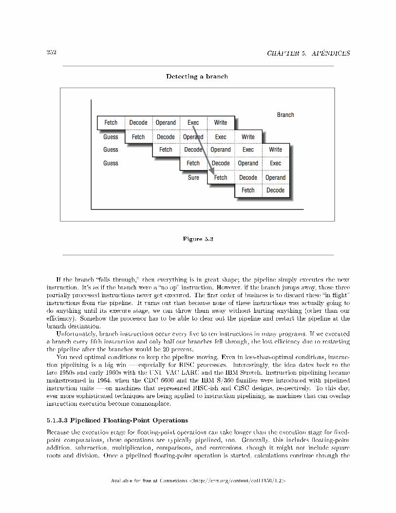
252 CHAPTER 5. APÉNDICES
Detecting a branch
Figure 5.3
If the branch �falls through,� then everything is in great shape; the pipeline simply executes the nextinstruction. It's as if the branch were a �no-op� instruction. However, if the branch jumps away, those threepartially processed instructions never get executed. The �rst order of business is to discard these �in-�ight�instructions from the pipeline. It turns out that because none of these instructions was actually going todo anything until its execute stage, we can throw them away without hurting anything (other than oure�ciency). Somehow the processor has to be able to clear out the pipeline and restart the pipeline at thebranch destination.
Unfortunately, branch instructions occur every �ve to ten instructions in many programs. If we executeda branch every �fth instruction and only half our branches fell through, the lost e�ciency due to restartingthe pipeline after the branches would be 20 percent.
You need optimal conditions to keep the pipeline moving. Even in less-than-optimal conditions, instruc-tion pipelining is a big win � especially for RISC processors. Interestingly, the idea dates back to thelate 1950s and early 1960s with the UNI- VAC LARC and the IBM Stretch. Instruction pipelining becamemainstreamed in 1964, when the CDC 6600 and the IBM S/360 families were introduced with pipelinedinstruction units � on machines that represented RISC-ish and CISC designs, respectively. To this day,ever more sophisticated techniques are being applied to instruction pipelining, as machines that can overlapinstruction execution become commonplace.
5.1.3.3 Pipelined Floating-Point Operations
Because the execution stage for �oating-point operations can take longer than the execution stage for �xed-point computations, these operations are typically pipelined, too. Generally, this includes �oating-pointaddition, subtraction, multiplication, comparisons, and conversions, though it might not include squareroots and division. Once a pipelined �oating-point operation is started, calculations continue through the
Available for free at Connexions <http://cnx.org/content/col11356/1.2>
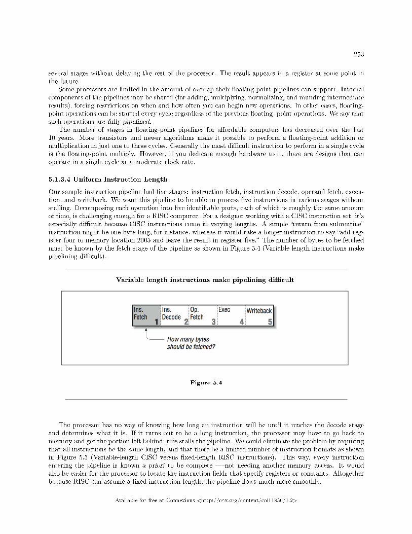
253
several stages without delaying the rest of the processor. The result appears in a register at some point inthe future.
Some processors are limited in the amount of overlap their �oating-point pipelines can support. Internalcomponents of the pipelines may be shared (for adding, multiplying, normalizing, and rounding intermediateresults), forcing restrictions on when and how often you can begin new operations. In other cases, �oating-point operations can be started every cycle regardless of the previous �oating- point operations. We say thatsuch operations are fully pipelined.
The number of stages in �oating-point pipelines for a�ordable computers has decreased over the last10 years. More transistors and newer algorithms make it possible to perform a �oating-point addition ormultiplication in just one to three cycles. Generally the most di�cult instruction to perform in a single cycleis the �oating-point multiply. However, if you dedicate enough hardware to it, there are designs that canoperate in a single cycle at a moderate clock rate.
5.1.3.4 Uniform Instruction Length
Our sample instruction pipeline had �ve stages: instruction fetch, instruction decode, operand fetch, execu-tion, and writeback. We want this pipeline to be able to process �ve instructions in various stages withoutstalling. Decomposing each operation into �ve identi�able parts, each of which is roughly the same amountof time, is challenging enough for a RISC computer. For a designer working with a CISC instruction set, it'sespecially di�cult because CISC instructions come in varying lengths. A simple �return from subroutine�instruction might be one byte long, for instance, whereas it would take a longer instruction to say �add reg-ister four to memory location 2005 and leave the result in register �ve.� The number of bytes to be fetchedmust be known by the fetch stage of the pipeline as shown in Figure 5.4 (Variable length instructions makepipelining di�cult).
Variable length instructions make pipelining di�cult
Figure 5.4
The processor has no way of knowing how long an instruction will be until it reaches the decode stageand determines what it is. If it turns out to be a long instruction, the processor may have to go back tomemory and get the portion left behind; this stalls the pipeline. We could eliminate the problem by requiringthat all instructions be the same length, and that there be a limited number of instruction formats as shownin Figure 5.5 (Variable-length CISC versus �xed-length RISC instructions). This way, every instructionentering the pipeline is known a priori to be complete � not needing another memory access. It wouldalso be easier for the processor to locate the instruction �elds that specify registers or constants. Altogetherbecause RISC can assume a �xed instruction length, the pipeline �ows much more smoothly.
Available for free at Connexions <http://cnx.org/content/col11356/1.2>
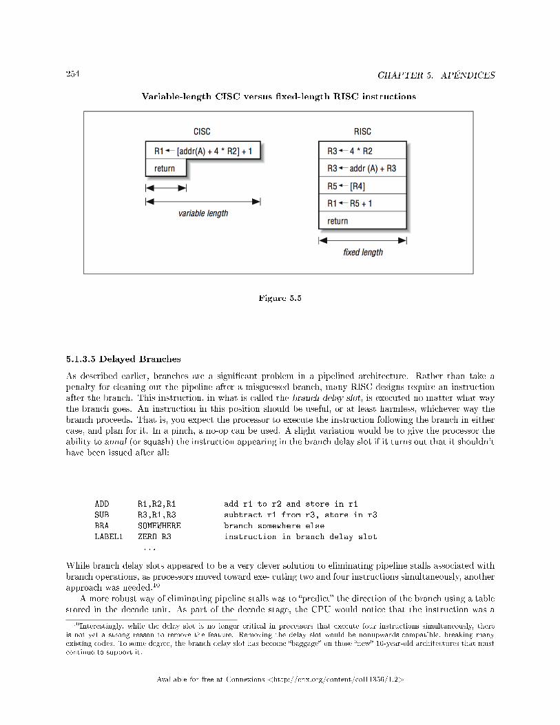
254 CHAPTER 5. APÉNDICES
Variable-length CISC versus �xed-length RISC instructions
Figure 5.5
5.1.3.5 Delayed Branches
As described earlier, branches are a signi�cant problem in a pipelined architecture. Rather than take apenalty for cleaning out the pipeline after a misguessed branch, many RISC designs require an instructionafter the branch. This instruction, in what is called the branch delay slot, is executed no matter what waythe branch goes. An instruction in this position should be useful, or at least harmless, whichever way thebranch proceeds. That is, you expect the processor to execute the instruction following the branch in eithercase, and plan for it. In a pinch, a no-op can be used. A slight variation would be to give the processor theability to annul (or squash) the instruction appearing in the branch delay slot if it turns out that it shouldn'thave been issued after all:
ADD R1,R2,R1 add r1 to r2 and store in r1
SUB R3,R1,R3 subtract r1 from r3, store in r3
BRA SOMEWHERE branch somewhere else
LABEL1 ZERO R3 instruction in branch delay slot
...
While branch delay slots appeared to be a very clever solution to eliminating pipeline stalls associated withbranch operations, as processors moved toward exe- cuting two and four instructions simultaneously, anotherapproach was needed.10
A more robust way of eliminating pipeline stalls was to �predict� the direction of the branch using a tablestored in the decode unit. As part of the decode stage, the CPU would notice that the instruction was a
10Interestingly, while the delay slot is no longer critical in processors that execute four instructions simultaneously, thereis not yet a strong reason to remove the feature. Removing the delay slot would be nonupwards-compatible, breaking manyexisting codes. To some degree, the branch delay slot has become �baggage� on those �new� 10-year-old architectures that mustcontinue to support it.
Available for free at Connexions <http://cnx.org/content/col11356/1.2>

255
branch and consult a table that kept the recent behavior of the branch; it would then make a guess. Basedon the guess, the CPU would immediately begin fetching at the predicted location. As long as the guesseswere correct, branches cost exactly the same as any other instruction.
If the prediction was wrong, the instructions that were in process had to be can- celled, resulting inwasted time and e�ort. A simple branch prediction scheme is typically correct well over 90% of the time,signi�cantly reducing the overall negative performance impact of pipeline stalls due to branches. All recentRISC designs incorporate some type of branch prediction, making branch delay slots e�ectively unnecessary.
Another mechanism for reducing branch penalties is conditional execution. These are instructions thatlook like branches in source code, but turn out to be a special type of instruction in the object code. They arevery useful because they replace test and branch sequences altogether. The following lines of code capturethe sense of a conditional branch:
IF ( B < C ) THEN
A = D
ELSE
A = E
ENDIF
Using branches, this would require at least two branches to ensure that the proper value ended up in A.Using conditional execution, one might generate code that looks as follows:
COMPARE B < C
IF TRUE A = D conditional instruction
IF FALSE A = E conditional instruction
This is a sequence of three instructions with no branches. One of the two assignments executes, and theother acts as a no-op. No branch prediction is needed, and the pipeline operates perfectly. There is a costto taking this approach when there are a large number of instructions in one or the other branch paths thatwould seldom get executed using the traditional branch instruction model.
5.1.3.6 Load/Store Architecture
In a load/store instruction set architecture, memory references are limited to explicit load and store instruc-tions. Each instruction may not make more than one memory reference per instruction. In a CISC processor,arithmetic and logical instructions can include embedded memory references. There are three reasons whylimiting loads and stores to their own instructions is an improvement:
• First, we want all instructions to be the same length, for the reasons given above. However, �xedlengths impose a budget limit when it comes to describing what the operation does and which registersit uses. An instruction that both referenced memory and performed some calculation wouldn't �twithin one instruction word.
• Second, giving every instruction the option to reference memory would com- plicate the pipeline becausethere would be two computations to perform� the address calculation plus whatever the instructionis supposed to do � but there is only one execution stage. We could throw more hardware at it,but by restricting memory references to explicit loads and stores, we can avoid the problem entirely.Any instruction can perform an address calculation or some other operation, but no instruction cando both.
Available for free at Connexions <http://cnx.org/content/col11356/1.2>
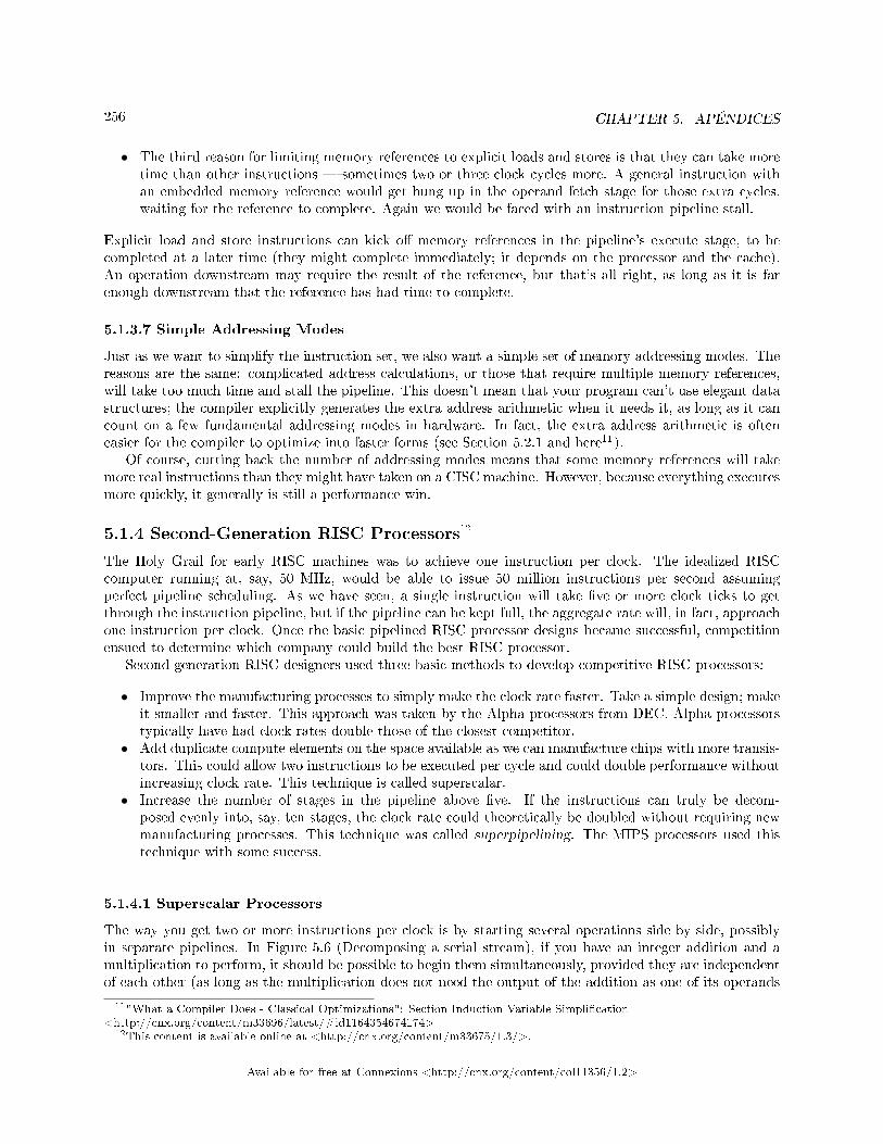
256 CHAPTER 5. APÉNDICES
• The third reason for limiting memory references to explicit loads and stores is that they can take moretime than other instructions � sometimes two or three clock cycles more. A general instruction withan embedded memory reference would get hung up in the operand fetch stage for those extra cycles,waiting for the reference to complete. Again we would be faced with an instruction pipeline stall.
Explicit load and store instructions can kick o� memory references in the pipeline's execute stage, to becompleted at a later time (they might complete immediately; it depends on the processor and the cache).An operation downstream may require the result of the reference, but that's all right, as long as it is farenough downstream that the reference has had time to complete.
5.1.3.7 Simple Addressing Modes
Just as we want to simplify the instruction set, we also want a simple set of memory addressing modes. Thereasons are the same: complicated address calculations, or those that require multiple memory references,will take too much time and stall the pipeline. This doesn't mean that your program can't use elegant datastructures; the compiler explicitly generates the extra address arithmetic when it needs it, as long as it cancount on a few fundamental addressing modes in hardware. In fact, the extra address arithmetic is ofteneasier for the compiler to optimize into faster forms (see Section 5.2.1 and here11).
Of course, cutting back the number of addressing modes means that some memory references will takemore real instructions than they might have taken on a CISC machine. However, because everything executesmore quickly, it generally is still a performance win.
5.1.4 Second-Generation RISC Processors12
The Holy Grail for early RISC machines was to achieve one instruction per clock. The idealized RISCcomputer running at, say, 50 MHz, would be able to issue 50 million instructions per second assumingperfect pipeline scheduling. As we have seen, a single instruction will take �ve or more clock ticks to getthrough the instruction pipeline, but if the pipeline can be kept full, the aggregate rate will, in fact, approachone instruction per clock. Once the basic pipelined RISC processor designs became successful, competitionensued to determine which company could build the best RISC processor.
Second-generation RISC designers used three basic methods to develop competitive RISC processors:
• Improve the manufacturing processes to simply make the clock rate faster. Take a simple design; makeit smaller and faster. This approach was taken by the Alpha processors from DEC. Alpha processorstypically have had clock rates double those of the closest competitor.
• Add duplicate compute elements on the space available as we can manufacture chips with more transis-tors. This could allow two instructions to be executed per cycle and could double performance withoutincreasing clock rate. This technique is called superscalar.
• Increase the number of stages in the pipeline above �ve. If the instructions can truly be decom-posed evenly into, say, ten stages, the clock rate could theoretically be doubled without requiring newmanufacturing processes. This technique was called superpipelining. The MIPS processors used thistechnique with some success.
5.1.4.1 Superscalar Processors
The way you get two or more instructions per clock is by starting several operations side by side, possiblyin separate pipelines. In Figure 5.6 (Decomposing a serial stream), if you have an integer addition and amultiplication to perform, it should be possible to begin them simultaneously, provided they are independentof each other (as long as the multiplication does not need the output of the addition as one of its operands
11"What a Compiler Does - Classical Optimizations": Section Induction Variable Simpli�cation<http://cnx.org/content/m33696/latest/#id1164354674174>
12This content is available online at <http://cnx.org/content/m33675/1.3/>.
Available for free at Connexions <http://cnx.org/content/col11356/1.2>

257
or vice versa). You could also execute multiple �xed-point instructions � compares, integer additions, etc.� at the same time, provided that they, too, are independent. Another term used to describe superscalarprocessors is multiple instruction issue processors.
Decomposing a serial stream
Figure 5.6
The number and variety of operations that can be run in parallel depends on both the program andthe processor. The program has to have enough usable parallelism so that there are multiple things to do,and the processor has to have an appropriate assortment of functional units and the ability to keep thembusy. The idea is conceptually simple, but it can be a challenge for both hardware designers and compilerwriters. Every opportunity to do several things in parallel exposes the danger of violating some precedence(i.e., performing computations in the wrong order).
5.1.4.2 Superpipelined Processors
Roughly stated, simpler circuitry can run at higher clock speeds. Put yourself in the role of a CPU designeragain. Looking at the instruction pipeline of your processor, you might decide that the reason you can't getmore speed out of it is that some of the stages are too complicated or have too much going on, and they areplacing limits on how fast the whole pipeline can go. Because the stages are clocked in unison, the slowestof them forms a weak link in the chain.
If you divide the complicated stages into less complicated portions, you can increase the overall speedof the pipeline. This is called superpipelining. More instruction pipeline stages with less complexity perstage will do the same work as a pipelined processor, but with higher throughput due to increased clockspeed. Figure 5.7 (MIPS R4000 instruction pipeline) shows an eight-stage pipeline used in the MIPS R4000processor.
Available for free at Connexions <http://cnx.org/content/col11356/1.2>
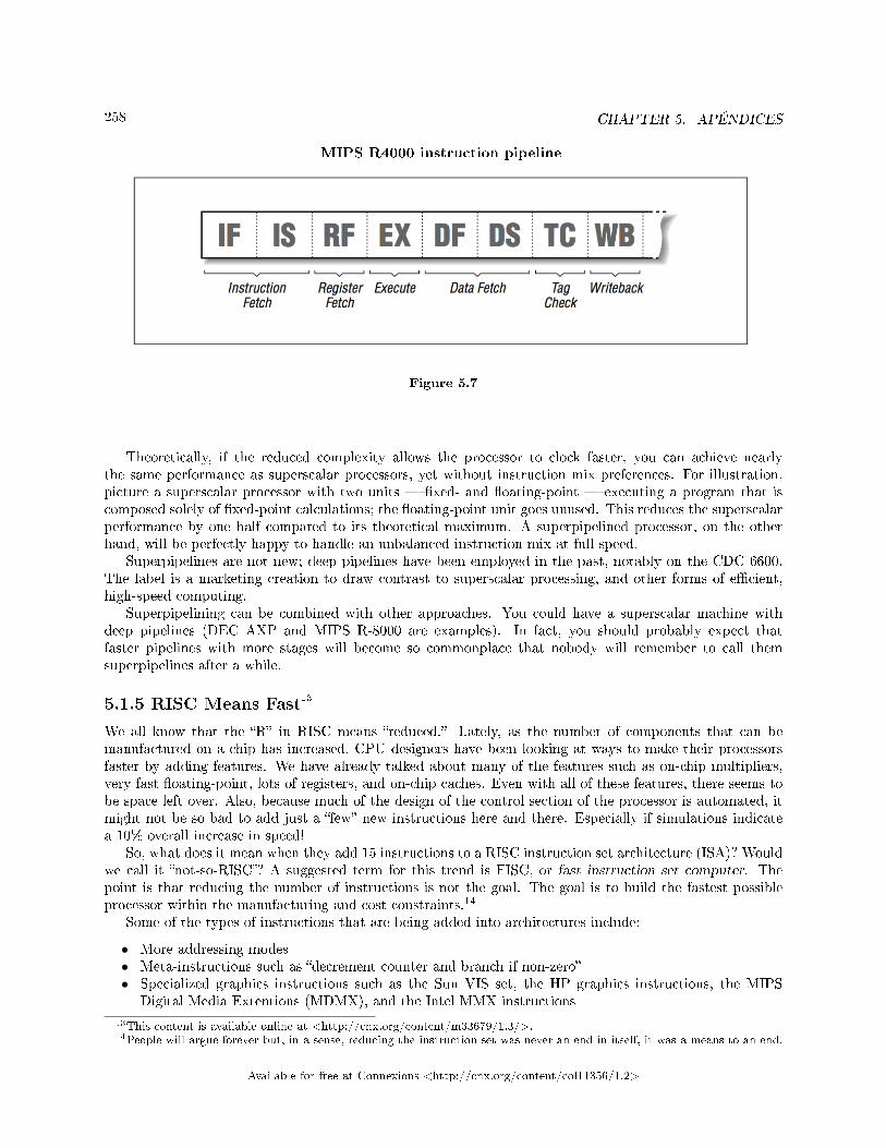
258 CHAPTER 5. APÉNDICES
MIPS R4000 instruction pipeline
Figure 5.7
Theoretically, if the reduced complexity allows the processor to clock faster, you can achieve nearlythe same performance as superscalar processors, yet without instruction mix preferences. For illustration,picture a superscalar processor with two units � �xed- and �oating-point � executing a program that iscomposed solely of �xed-point calculations; the �oating-point unit goes unused. This reduces the superscalarperformance by one half compared to its theoretical maximum. A superpipelined processor, on the otherhand, will be perfectly happy to handle an unbalanced instruction mix at full speed.
Superpipelines are not new; deep pipelines have been employed in the past, notably on the CDC 6600.The label is a marketing creation to draw contrast to superscalar processing, and other forms of e�cient,high-speed computing.
Superpipelining can be combined with other approaches. You could have a superscalar machine withdeep pipelines (DEC AXP and MIPS R-8000 are examples). In fact, you should probably expect thatfaster pipelines with more stages will become so commonplace that nobody will remember to call themsuperpipelines after a while.
5.1.5 RISC Means Fast13
We all know that the �R� in RISC means �reduced.� Lately, as the number of components that can bemanufactured on a chip has increased, CPU designers have been looking at ways to make their processorsfaster by adding features. We have already talked about many of the features such as on-chip multipliers,very fast �oating-point, lots of registers, and on-chip caches. Even with all of these features, there seems tobe space left over. Also, because much of the design of the control section of the processor is automated, itmight not be so bad to add just a �few� new instructions here and there. Especially if simulations indicatea 10% overall increase in speed!
So, what does it mean when they add 15 instructions to a RISC instruction set architecture (ISA)? Wouldwe call it �not-so-RISC�? A suggested term for this trend is FISC, or fast instruction set computer. Thepoint is that reducing the number of instructions is not the goal. The goal is to build the fastest possibleprocessor within the manufacturing and cost constraints.14
Some of the types of instructions that are being added into architectures include:
• More addressing modes• Meta-instructions such as �decrement counter and branch if non-zero�• Specialized graphics instructions such as the Sun VIS set, the HP graphics instructions, the MIPS
Digital Media Extentions (MDMX), and the Intel MMX instructions
13This content is available online at <http://cnx.org/content/m33679/1.3/>.14People will argue forever but, in a sense, reducing the instruction set was never an end in itself, it was a means to an end.
Available for free at Connexions <http://cnx.org/content/col11356/1.2>
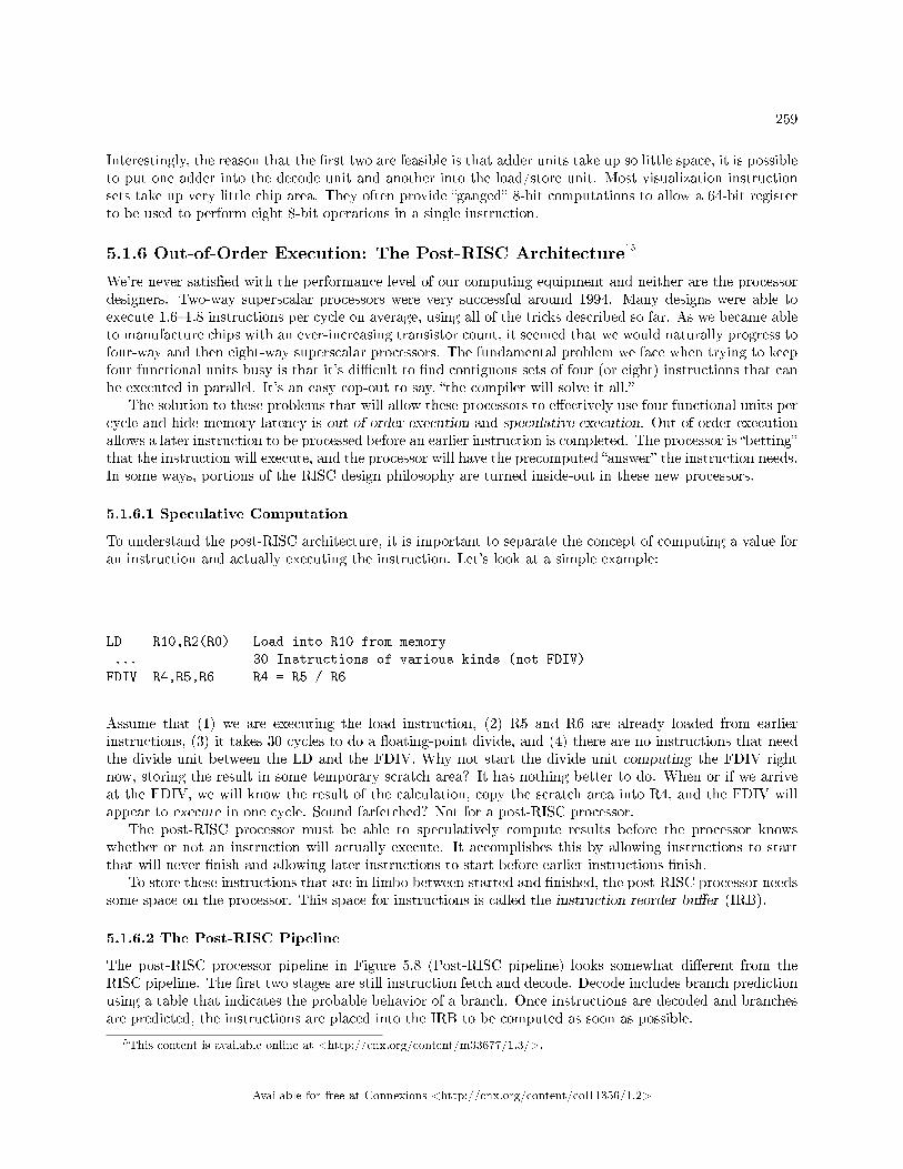
259
Interestingly, the reason that the �rst two are feasible is that adder units take up so little space, it is possibleto put one adder into the decode unit and another into the load/store unit. Most visualization instructionsets take up very little chip area. They often provide �ganged� 8-bit computations to allow a 64-bit registerto be used to perform eight 8-bit operations in a single instruction.
5.1.6 Out-of-Order Execution: The Post-RISC Architecture15
We're never satis�ed with the performance level of our computing equipment and neither are the processordesigners. Two-way superscalar processors were very successful around 1994. Many designs were able toexecute 1.6�1.8 instructions per cycle on average, using all of the tricks described so far. As we became ableto manufacture chips with an ever-increasing transistor count, it seemed that we would naturally progress tofour-way and then eight-way superscalar processors. The fundamental problem we face when trying to keepfour functional units busy is that it's di�cult to �nd contiguous sets of four (or eight) instructions that canbe executed in parallel. It's an easy cop-out to say, �the compiler will solve it all.�
The solution to these problems that will allow these processors to e�ectively use four functional units percycle and hide memory latency is out-of-order execution and speculative execution. Out-of-order executionallows a later instruction to be processed before an earlier instruction is completed. The processor is �betting�that the instruction will execute, and the processor will have the precomputed �answer� the instruction needs.In some ways, portions of the RISC design philosophy are turned inside-out in these new processors.
5.1.6.1 Speculative Computation
To understand the post-RISC architecture, it is important to separate the concept of computing a value foran instruction and actually executing the instruction. Let's look at a simple example:
LD R10,R2(R0) Load into R10 from memory
... 30 Instructions of various kinds (not FDIV)
FDIV R4,R5,R6 R4 = R5 / R6
Assume that (1) we are executing the load instruction, (2) R5 and R6 are already loaded from earlierinstructions, (3) it takes 30 cycles to do a �oating-point divide, and (4) there are no instructions that needthe divide unit between the LD and the FDIV. Why not start the divide unit computing the FDIV rightnow, storing the result in some temporary scratch area? It has nothing better to do. When or if we arriveat the FDIV, we will know the result of the calculation, copy the scratch area into R4, and the FDIV willappear to execute in one cycle. Sound farfetched? Not for a post-RISC processor.
The post-RISC processor must be able to speculatively compute results before the processor knowswhether or not an instruction will actually execute. It accomplishes this by allowing instructions to startthat will never �nish and allowing later instructions to start before earlier instructions �nish.
To store these instructions that are in limbo between started and �nished, the post-RISC processor needssome space on the processor. This space for instructions is called the instruction reorder bu�er (IRB).
5.1.6.2 The Post-RISC Pipeline
The post-RISC processor pipeline in Figure 5.8 (Post-RISC pipeline) looks somewhat di�erent from theRISC pipeline. The �rst two stages are still instruction fetch and decode. Decode includes branch predictionusing a table that indicates the probable behavior of a branch. Once instructions are decoded and branchesare predicted, the instructions are placed into the IRB to be computed as soon as possible.
15This content is available online at <http://cnx.org/content/m33677/1.3/>.
Available for free at Connexions <http://cnx.org/content/col11356/1.2>
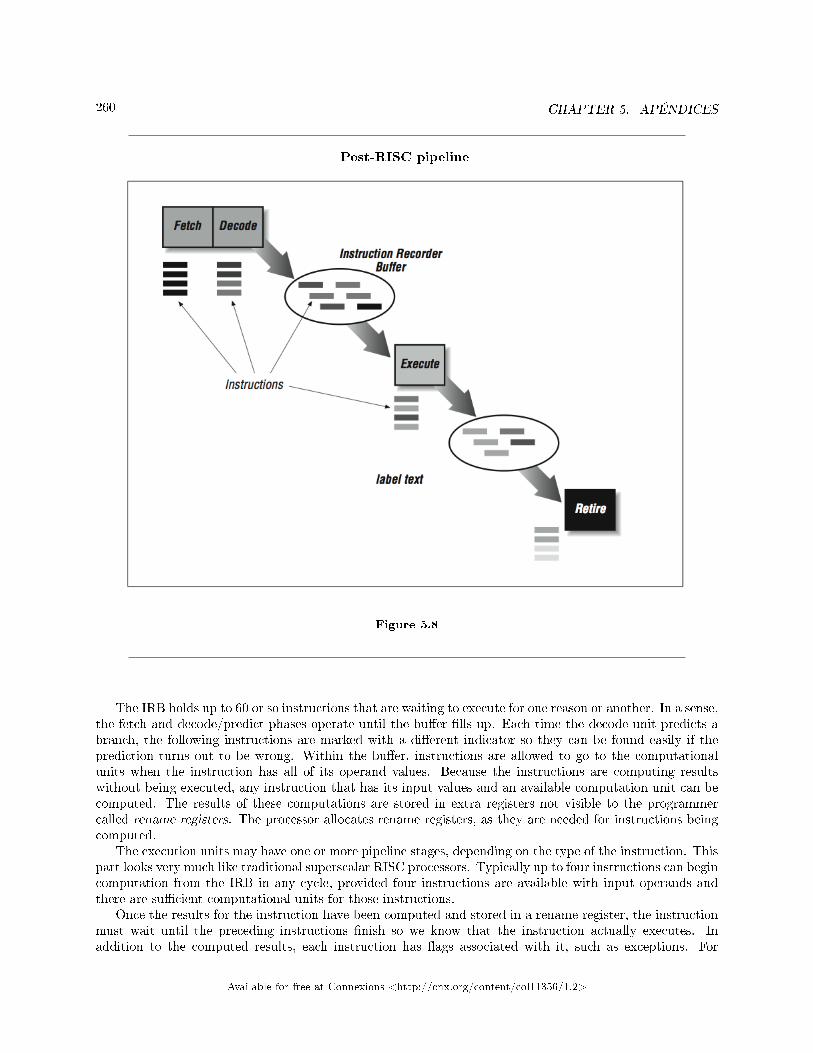
260 CHAPTER 5. APÉNDICES
Post-RISC pipeline
Figure 5.8
The IRB holds up to 60 or so instructions that are waiting to execute for one reason or another. In a sense,the fetch and decode/predict phases operate until the bu�er �lls up. Each time the decode unit predicts abranch, the following instructions are marked with a di�erent indicator so they can be found easily if theprediction turns out to be wrong. Within the bu�er, instructions are allowed to go to the computationalunits when the instruction has all of its operand values. Because the instructions are computing resultswithout being executed, any instruction that has its input values and an available computation unit can becomputed. The results of these computations are stored in extra registers not visible to the programmercalled rename registers. The processor allocates rename registers, as they are needed for instructions beingcomputed.
The execution units may have one or more pipeline stages, depending on the type of the instruction. Thispart looks very much like traditional superscalar RISC processors. Typically up to four instructions can begincomputation from the IRB in any cycle, provided four instructions are available with input operands andthere are su�cient computational units for those instructions.
Once the results for the instruction have been computed and stored in a rename register, the instructionmust wait until the preceding instructions �nish so we know that the instruction actually executes. Inaddition to the computed results, each instruction has �ags associated with it, such as exceptions. For
Available for free at Connexions <http://cnx.org/content/col11356/1.2>
261
example, you would not be happy if your program crashed with the following message: �Error, divide byzero. I was precomputing a divide in case you got to the instruction to save some time, but the branchwas mispredicted and it turned out that you were never going to execute that divide anyway. I still had toblow you up though. No hard feelings? Signed, the post-RISC CPU.� So when a speculatively computedinstruction divides by zero, the CPU must simply store that fact until it knows the instruction will executeand at that moment, the program can be legitimately crashed.
If a branch does get mispredicted, a lot of bookkeeping must occur very quickly. A message is sent to allthe units to discard instructions that are part of all control �ow paths beyond the incorrect branch.
Instead of calling the last phase of the pipeline �writeback,� it's called �retire.� The retire phase is what�executes� the instructions that have already been computed. The retire phase keeps track of the instructionexecution order and retires the instructions in program order, posting results from the rename registers tothe actual registers and raising exceptions as necessary. Typically up to four instructions can be retired percycle.
So the post-RISC pipeline is actually three pipelines connected by two bu�ers that allow instructions tobe processed out of order. However, even with all of this speculative computation going on, the retire unitforces the processor to appear as a simple RISC processor with predictable execution and interrupts.
5.1.7 Closing Notes16
Congratulations for reaching the end of a long chapter! We have talked a little bit about old computers,CISC, RISC, post-RISC, and EPIC, and mentioned supercomputers in passing. I think it's interesting toobserve that RISC processors are a branch o� a long-established tree. Many of the ideas that have gone intoRISC designs are borrowed from other types of computers, but none of them evolved into RISC � RISCstarted at a discontinuity. There were hints of a RISC revolution (the CDC 6600 and the IBM 801 project)but it really was forced on the world (for its own good) by CPU designers at Berkeley and Stanford in the1980s.
As RISC has matured, there have been many improvements. Each time it appears that we have reachedthe limit of the performance of our microprocessors there is a new architectural breakthrough improving oursingle CPU performance. How long can it continue? It is clear that as long as competition continues, thereis signi�cant performance headroom using the out-of-order execution as the clock rates move from a typical200 MHz to 500+ MHz. DEC's Alpha 21264 is planned to have four-way out-of-order execution at 500 MHzby 1998. As of 1998, vendors are beginning to reveal their plans for processors clocked at 1000 MHz or 1GHz.
Unfortunately, developing a new processor is a very expensive task. If enough companies merge andcompetition diminishes, the rate of innovation will slow. Hopefully we will be seeing four processors on achip, each 16-way out-of-order superscalar, clocked at 1 GHz for $200 before we eliminate competition andlet the CPU designers rest on their laurels. At that point, scalable parallel processing will suddenly becomeinteresting again.
How will designers tackle some of the fundamental architectural problems, perhaps the largest beingmemory systems? Even though the post-RISC architecture and the EPIC alleviate the latency problemssomewhat, the memory bottleneck will always be there. The good news is that even though memoryperformance improves more slowly than CPU performance, memory system performance does improve overtime. We'll look next at techniques for building memory systems.
As discussed in here17, the exercises that come at the end of most chapters in this book are not like theexercises in most engineering texts. These exercises are mostly thought experiments, without well-de�nedanswers, designed to get you thinking about the hardware on your desk.
16This content is available online at <http://cnx.org/content/m33683/1.3/>.17"Introduction to High Performance Computing" <http://cnx.org/content/m32676/latest/>
Available for free at Connexions <http://cnx.org/content/col11356/1.2>
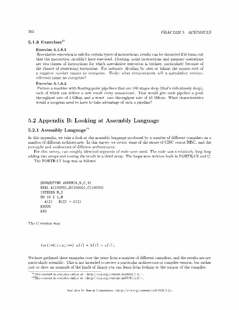
262 CHAPTER 5. APÉNDICES
5.1.8 Exercises18
Exercise 5.1.8.1Speculative execution is safe for certain types of instructions; results can be discarded if it turns outthat the instruction shouldn't have executed. Floating- point instructions and memory operationsare two classes of instructions for which speculative execution is trickier, particularly because ofthe chance of generating exceptions. For instance, dividing by zero or taking the square root ofa negative number causes an exception. Under what circumstances will a speculative memoryreference cause an exception?
Exercise 5.1.8.2Picture a machine with �oating-point pipelines that are 100 stages deep (that's ridiculously deep),each of which can deliver a new result every nanosecond. That would give each pipeline a peakthroughput rate of 1 G�op, and a worst- case throughput rate of 10 M�ops. What characteristicswould a program need to have to take advantage of such a pipeline?
5.2 Appendix B: Looking at Assembly Language
5.2.1 Assembly Language19
In this appendix, we take a look at the assembly language produced by a number of di�erent compilers on anumber of di�erent architectures. In this survey we revisit some of the issues of CISC versus RISC, and thestrengths and weaknesses of di�erent architectures.
For this survey, two roughly identical segments of code were used. The code was a relatively long loopadding two arrays and storing the result in a third array. The loops were written both in FORTRAN and C.
The FORTRAN loop was as follows:
SUBROUTINE ADDEM(A,B,C,N)
REAL A(10000),B(10000),C(10000)
INTEGER N,I
DO 10 I=1,N
A(I) = B(I) + C(I)
ENDDO
END
The C version was:
for(i=0;i<n;i++) a[i] = b[i] + c[i];
We have gathered these examples over the years from a number of di�erent compilers, and the results are notparticularly scienti�c. This is not intended to review a particular architecture or compiler version, but ratherjust to show an example of the kinds of things you can learn from looking at the output of the compiler.
18This content is available online at <http://cnx.org/content/m33682/1.3/>.19This content is available online at <http://cnx.org/content/m33787/1.3/>.
Available for free at Connexions <http://cnx.org/content/col11356/1.2>
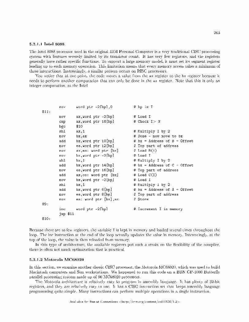
263
5.2.1.1 Intel 8088
The Intel 8088 processor used in the original IBM Personal Computer is a very traditional CISC processingsystem with features severely limited by its transistor count. It has very few registers, and the registersgenerally have rather speci�c functions. To support a large memory model, it must set its segment registerleading up to each memory operation. This limitation means that every memory access takes a minimum ofthree instructions. Interestingly, a similar pattern occurs on RISC processors.
You notice that at one point, the code moves a value from the ax register to the bx register because itneeds to perform another computation that can only be done in the ax register. Note that this is only aninteger computation, as the Intel
mov word ptr -2[bp],0 # bp is I
$11:
mov ax,word ptr -2[bp] # Load I
cmp ax,word ptr 18[bp] # Check I>=N
bge $10
shl ax,1 # Multiply I by 2
mov bx,ax # Done - now move to bx
add bx,word ptr 10[bp] # bx = Address of B + Offset
mov es,word ptr 12[bp] # Top part of address
mov ax,es: word ptr [bx] # Load B(i)
mov bx,word ptr -2[bp] # Load I
shl bx,1 # Multiply I by 2
add bx,word ptr 14[bp] # bx = Address of C + Offset
mov es,word ptr 16[bp] # Top part of address
add ax,es: word ptr [bx] # Load C(I)
mov bx,word ptr -2[bp] # Load I
shl bx,1 # Multiply I by 2
add bx,word ptr 6[bp] # bx = Address of A + Offset
mov es,word ptr 8[bp] # Top part of address
mov es: word ptr [bx],ax # Store
$9:
inc word ptr -2[bp] # Increment I in memory
jmp $11
$10:
Because there are so few registers, the variable I is kept in memory and loaded several times throughout theloop. The inc instruction at the end of the loop actually updates the value in memory. Interestingly, at thetop of the loop, the value is then reloaded from memory.
In this type of architecture, the available registers put such a strain on the �exibility of the compiler,there is often not much optimization that is practical.
5.2.1.2 Motorola MC68020
In this section, we examine another classic CISC processor, the Motorola MC68020, which was used to buildMacintosh computers and Sun workstations. We happened to run this code on a BBN GP-1000 Butter�yparallel processing system made up of 96 MC68020 processors.
The Motorola architecture is relatively easy to program in assembly language. It has plenty of 32-bitregisters, and they are relatively easy to use. It has a CISC instruction set that keeps assembly languageprogramming quite simple. Many instructions can perform multiple operations in a single instruction.
Available for free at Connexions <http://cnx.org/content/col11356/1.2>
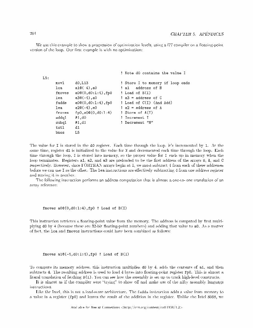
264 CHAPTER 5. APÉNDICES
We use this example to show a progression of optimization levels, using a f77 compiler on a �oating-pointversion of the loop. Our �rst example is with no optimization:
! Note d0 contains the value I
L5:
movl d0,L13 ! Store I to memory if loop ends
lea a1@(-4),a0 ! a1 = address of B
fmoves a0@(0,d0:l:4),fp0 ! Load of B(I)
lea a3@(-4),a0 ! a3 = address of C
fadds a0@(0,d0:l:4),fp0 ! Load of C(I) (And Add)
lea a2@(-4),a0 ! a2 = address of A
fmoves fp0,a0@(0,d0:l:4) ! Store of A(I)
addql #1,d0 ! Increment I
subql #1,d1 ! Decrement "N"
tstl d1
bnes L5
The value for I is stored in the d0 register. Each time through the loop, it's incremented by 1. At thesame time, register d1 is initialized to the value for N and decremented each time through the loop. Eachtime through the loop, I is stored into memory, so the proper value for I ends up in memory when theloop terminates. Registers a1, a2, and a3 are preloaded to be the �rst address of the arrays B, A, and C
respectively. However, since FORTRAN arrays begin at 1, we must subtract 4 from each of these addressesbefore we can use I as the o�set. The lea instructions are e�ectively subtracting 4 from one address registerand storing it in another.
The following instruction performs an address computation that is almost a one-to- one translation of anarray reference:
fmoves a0@(0,d0:l:4),fp0 ! Load of B(I)
This instruction retrieves a �oating-point value from the memory. The address is computed by �rst multi-plying d0 by 4 (because these are 32-bit �oating-point numbers) and adding that value to a0. As a matterof fact, the lea and fmoves instructions could have been combined as follows:
fmoves a1@(-4,d0:l:4),fp0 ! Load of B(I)
To compute its memory address, this instruction multiplies d0 by 4, adds the contents of a1, and thensubtracts 4. The resulting address is used to load 4 bytes into �oating-point register fp0. This is almost aliteral translation of fetching B(I). You can see how the assembly is set up to track high-level constructs.
It is almost as if the compiler were �trying� to show o� and make use of the nifty assembly languageinstructions.
Like the Intel, this is not a load-store architecture. The fadds instruction adds a value from memory toa value in a register (fp0) and leaves the result of the addition in the register. Unlike the Intel 8088, we
Available for free at Connexions <http://cnx.org/content/col11356/1.2>
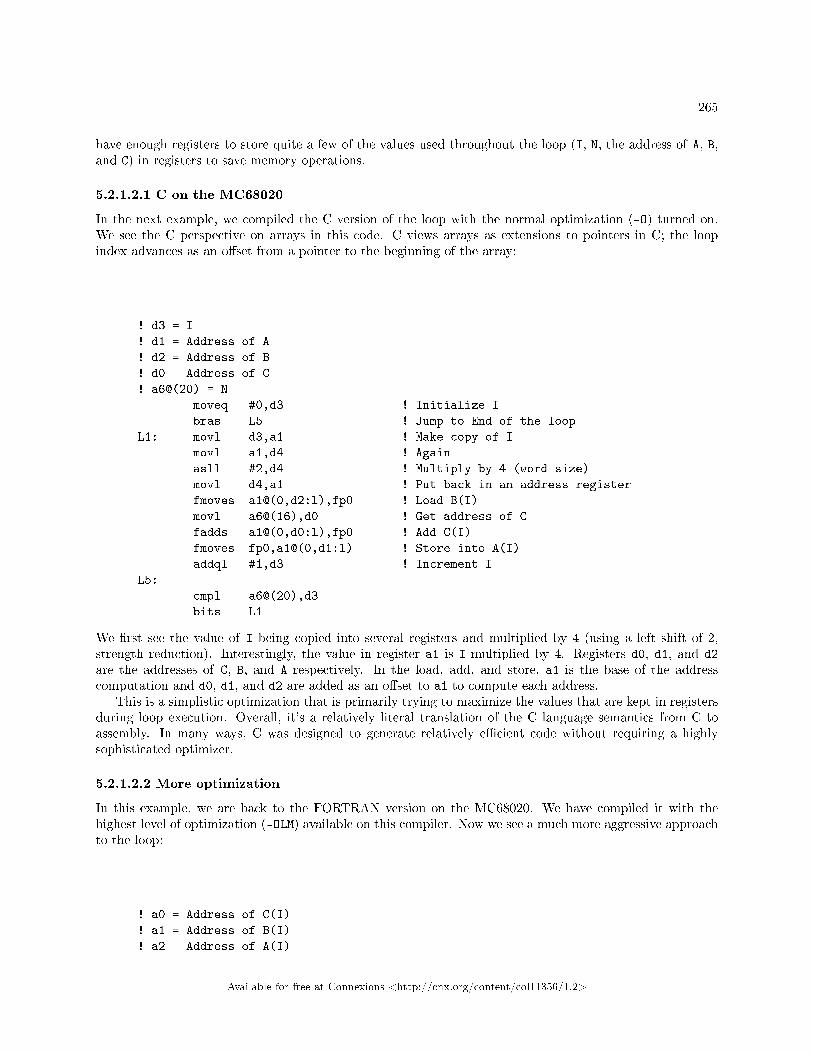
265
have enough registers to store quite a few of the values used throughout the loop (I, N, the address of A, B,and C) in registers to save memory operations.
5.2.1.2.1 C on the MC68020
In the next example, we compiled the C version of the loop with the normal optimization (-O) turned on.We see the C perspective on arrays in this code. C views arrays as extensions to pointers in C; the loopindex advances as an o�set from a pointer to the beginning of the array:
! d3 = I
! d1 = Address of A
! d2 = Address of B
! d0 = Address of C
! a6@(20) = N
moveq #0,d3 ! Initialize I
bras L5 ! Jump to End of the loop
L1: movl d3,a1 ! Make copy of I
movl a1,d4 ! Again
asll #2,d4 ! Multiply by 4 (word size)
movl d4,a1 ! Put back in an address register
fmoves a1@(0,d2:l),fp0 ! Load B(I)
movl a6@(16),d0 ! Get address of C
fadds a1@(0,d0:l),fp0 ! Add C(I)
fmoves fp0,a1@(0,d1:l) ! Store into A(I)
addql #1,d3 ! Increment I
L5:
cmpl a6@(20),d3
bits L1
We �rst see the value of I being copied into several registers and multiplied by 4 (using a left shift of 2,strength reduction). Interestingly, the value in register a1 is I multiplied by 4. Registers d0, d1, and d2
are the addresses of C, B, and A respectively. In the load, add, and store, a1 is the base of the addresscomputation and d0, d1, and d2 are added as an o�set to a1 to compute each address.
This is a simplistic optimization that is primarily trying to maximize the values that are kept in registersduring loop execution. Overall, it's a relatively literal translation of the C language semantics from C toassembly. In many ways, C was designed to generate relatively e�cient code without requiring a highlysophisticated optimizer.
5.2.1.2.2 More optimization
In this example, we are back to the FORTRAN version on the MC68020. We have compiled it with thehighest level of optimization (-OLM) available on this compiler. Now we see a much more aggressive approachto the loop:
! a0 = Address of C(I)
! a1 = Address of B(I)
! a2 = Address of A(I)
Available for free at Connexions <http://cnx.org/content/col11356/1.2>
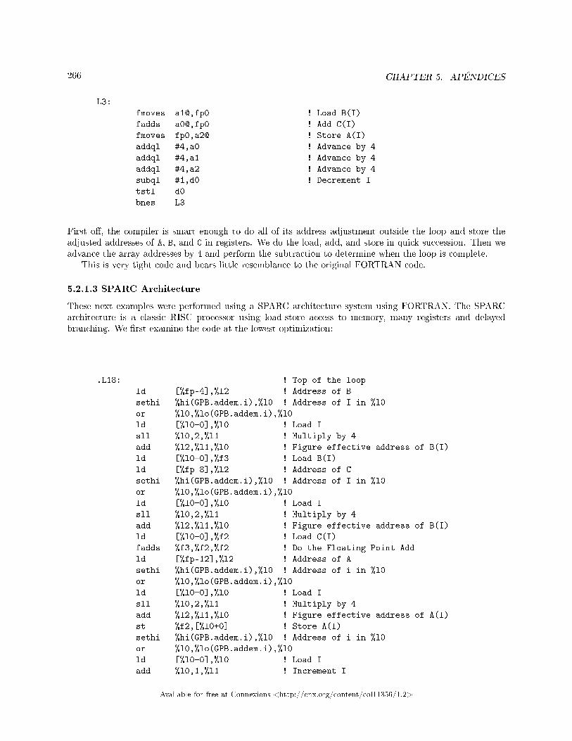
266 CHAPTER 5. APÉNDICES
L3:
fmoves a1@,fp0 ! Load B(I)
fadds a0@,fp0 ! Add C(I)
fmoves fp0,a2@ ! Store A(I)
addql #4,a0 ! Advance by 4
addql #4,a1 ! Advance by 4
addql #4,a2 ! Advance by 4
subql #1,d0 ! Decrement I
tstl d0
bnes L3
First o�, the compiler is smart enough to do all of its address adjustment outside the loop and store theadjusted addresses of A, B, and C in registers. We do the load, add, and store in quick succession. Then weadvance the array addresses by 4 and perform the subtraction to determine when the loop is complete.
This is very tight code and bears little resemblance to the original FORTRAN code.
5.2.1.3 SPARC Architecture
These next examples were performed using a SPARC architecture system using FORTRAN. The SPARCarchitecture is a classic RISC processor using load-store access to memory, many registers and delayedbranching. We �rst examine the code at the lowest optimization:
.L18: ! Top of the loop
ld [%fp-4],%l2 ! Address of B
sethi %hi(GPB.addem.i),%l0 ! Address of I in %l0
or %l0,%lo(GPB.addem.i),%l0
ld [%l0+0],%l0 ! Load I
sll %l0,2,%l1 ! Multiply by 4
add %l2,%l1,%l0 ! Figure effective address of B(I)
ld [%l0+0],%f3 ! Load B(I)
ld [%fp-8],%l2 ! Address of C
sethi %hi(GPB.addem.i),%l0 ! Address of I in %l0
or %l0,%lo(GPB.addem.i),%l0
ld [%l0+0],%l0 ! Load I
sll %l0,2,%l1 ! Multiply by 4
add %l2,%l1,%l0 ! Figure effective address of B(I)
ld [%l0+0],%f2 ! Load C(I)
fadds %f3,%f2,%f2 ! Do the Floating Point Add
ld [%fp-12],%l2 ! Address of A
sethi %hi(GPB.addem.i),%l0 ! Address of i in %l0
or %l0,%lo(GPB.addem.i),%l0
ld [%l0+0],%l0 ! Load I
sll %l0,2,%l1 ! Multiply by 4
add %l2,%l1,%l0 ! Figure effective address of A(I)
st %f2,[%l0+0] ! Store A(I)
sethi %hi(GPB.addem.i),%l0 ! Address of i in %l0
or %l0,%lo(GPB.addem.i),%l0
ld [%l0+0],%l0 ! Load I
add %l0,1,%l1 ! Increment I
Available for free at Connexions <http://cnx.org/content/col11356/1.2>
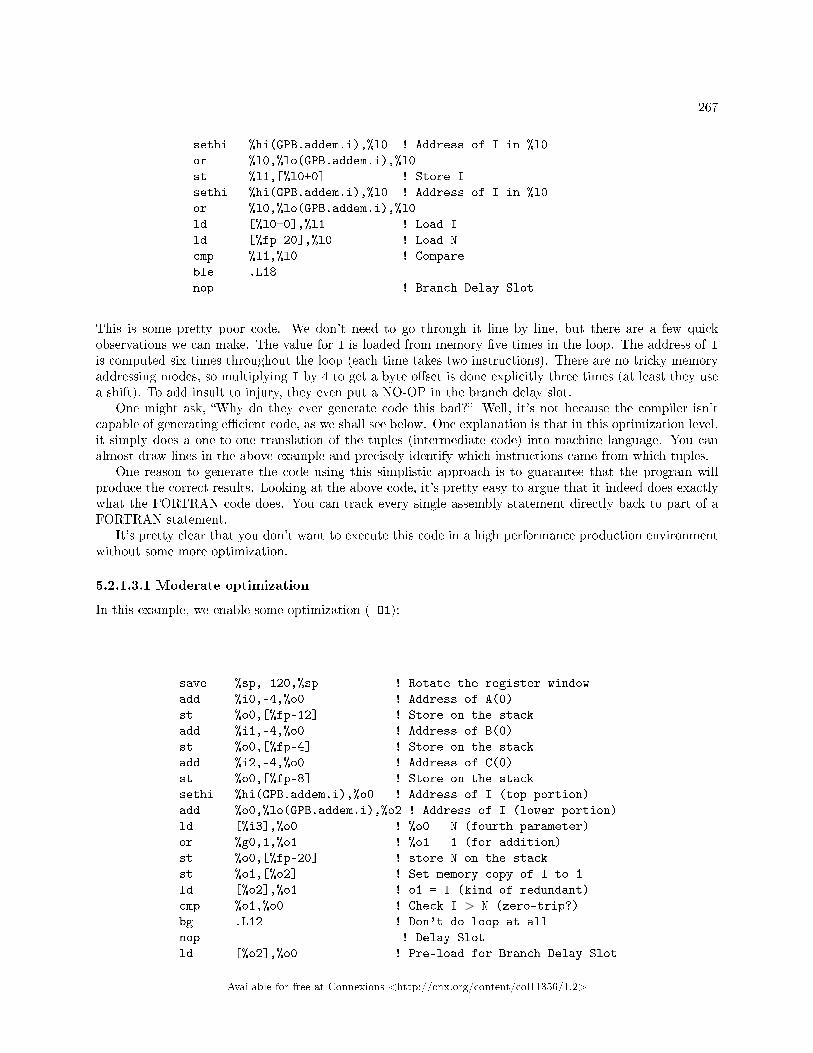
267
sethi %hi(GPB.addem.i),%l0 ! Address of I in %l0
or %l0,%lo(GPB.addem.i),%l0
st %l1,[%l0+0] ! Store I
sethi %hi(GPB.addem.i),%l0 ! Address of I in %l0
or %l0,%lo(GPB.addem.i),%l0
ld [%l0+0],%l1 ! Load I
ld [%fp-20],%l0 ! Load N
cmp %l1,%l0 ! Compare
ble .L18
nop ! Branch Delay Slot
This is some pretty poor code. We don't need to go through it line by line, but there are a few quickobservations we can make. The value for I is loaded from memory �ve times in the loop. The address of Iis computed six times throughout the loop (each time takes two instructions). There are no tricky memoryaddressing modes, so multiplying I by 4 to get a byte o�set is done explicitly three times (at least they usea shift). To add insult to injury, they even put a NO-OP in the branch delay slot.
One might ask, �Why do they ever generate code this bad?� Well, it's not because the compiler isn'tcapable of generating e�cient code, as we shall see below. One explanation is that in this optimization level,it simply does a one-to-one translation of the tuples (intermediate code) into machine language. You canalmost draw lines in the above example and precisely identify which instructions came from which tuples.
One reason to generate the code using this simplistic approach is to guarantee that the program willproduce the correct results. Looking at the above code, it's pretty easy to argue that it indeed does exactlywhat the FORTRAN code does. You can track every single assembly statement directly back to part of aFORTRAN statement.
It's pretty clear that you don't want to execute this code in a high performance production environmentwithout some more optimization.
5.2.1.3.1 Moderate optimization
In this example, we enable some optimization (-O1):
save %sp,-120,%sp ! Rotate the register window
add %i0,-4,%o0 ! Address of A(0)
st %o0,[%fp-12] ! Store on the stack
add %i1,-4,%o0 ! Address of B(0)
st %o0,[%fp-4] ! Store on the stack
add %i2,-4,%o0 ! Address of C(0)
st %o0,[%fp-8] ! Store on the stack
sethi %hi(GPB.addem.i),%o0 ! Address of I (top portion)
add %o0,%lo(GPB.addem.i),%o2 ! Address of I (lower portion)
ld [%i3],%o0 ! %o0 = N (fourth parameter)
or %g0,1,%o1 ! %o1 = 1 (for addition)
st %o0,[%fp-20] ! store N on the stack
st %o1,[%o2] ! Set memory copy of I to 1
ld [%o2],%o1 ! o1 = I (kind of redundant)
cmp %o1,%o0 ! Check I > N (zero-trip?)
bg .L12 ! Don't do loop at all
nop ! Delay Slot
ld [%o2],%o0 ! Pre-load for Branch Delay Slot
Available for free at Connexions <http://cnx.org/content/col11356/1.2>

268 CHAPTER 5. APÉNDICES
.L900000110: ! Top of the loop
ld [%fp-4],%o1 ! o1 = Address of B(0)
sll %o0,2,%o0 ! Multiply I by 4
ld [%o1+%o0],%f2 ! f2 = B(I)
ld [%o2],%o0 ! Load I from memory
ld [%fp-8],%o1 ! o1 = Address of C(0)
sll %o0,2,%o0 ! Multiply I by 4
ld [%o1+%o0],%f3 ! f3 = C(I)
fadds %f2,%f3,%f2 ! Register-to-register add
ld [%o2],%o0 ! Load I from memory (not again!)
ld [%fp-12],%o1 ! o1 = Address of A(0)
sll %o0,2,%o0 ! Multiply I by 4 (yes, again)
st %f2,[%o1+%o0] ! A(I) = f2
ld [%o2],%o0 ! Load I from memory
add %o0,1,%o0 ! Increment I in register
st %o0,[%o2] ! Store I back into memory
ld [%o2],%o0 ! Load I back into a register
ld [%fp-20],%o1 ! Load N into a register
cmp %o0,%o1 ! I > N ??
ble,a .L900000110
ld [%o2],%o0 ! Branch Delay Slot
This is a signi�cant improvement from the previous example. Some loop constant computations (subtracting4) were hoisted out of the loop. We only loaded I 4 times during a loop iteration. Strangely, the compilerdidn't choose to store the addresses of A(0), B(0), and C(0) in registers at all even though there were plentyof registers. Even more perplexing is the fact that it loaded a value from memory immediately after it hadstored it from the exact same register!
But one bright spot is the branch delay slot. For the �rst iteration, the load was done before the loopstarted. For the successive iterations, the �rst load was done in the branch delay slot at the bottom of theloop.
Comparing this code to the moderate optimization code on the MC68020, you can begin to get a senseof why RISC was not an overnight sensation. It turned out that an unsophisticated compiler could generatemuch tighter code for a CISC processor than a RISC processor. RISC processors are always executing extrainstructions here and there to compensate for the lack of slick features in their instruction set. If a processorhas a faster clock rate but has to execute more instructions, it does not always have better performance thana slower, more e�cient processor.
But as we shall soon see, this CISC advantage is about to evaporate in this particular example.
5.2.1.3.2 Higher optimization
We now increase the optimization to -O2. Now the compiler generates much better code. It's important youremember that this is the same compiler being used for all three examples.
At this optimization level, the compiler looked through the code su�ciently well to know it didn't evenneed to rotate the register windows (no save instruction). Clearly the compiler looked at the register usageof the entire routine:
! Note, didn't even rotate the register Window
! We just use the %o registers from the caller
Available for free at Connexions <http://cnx.org/content/col11356/1.2>
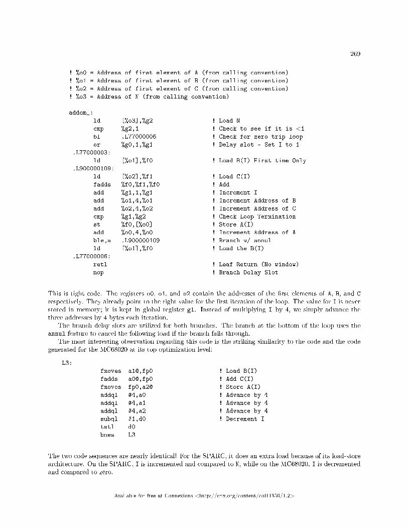
269
! %o0 = Address of first element of A (from calling convention)
! %o1 = Address of first element of B (from calling convention)
! %o2 = Address of first element of C (from calling convention)
! %o3 = Address of N (from calling convention)
addem_:
ld [%o3],%g2 ! Load N
cmp %g2,1 ! Check to see if it is <1
bl .L77000006 ! Check for zero trip loop
or %g0,1,%g1 ! Delay slot - Set I to 1
.L77000003:
ld [%o1],%f0 ! Load B(I) First time Only
.L900000109:
ld [%o2],%f1 ! Load C(I)
fadds %f0,%f1,%f0 ! Add
add %g1,1,%g1 ! Increment I
add %o1,4,%o1 ! Increment Address of B
add %o2,4,%o2 ! Increment Address of C
cmp %g1,%g2 ! Check Loop Termination
st %f0,[%o0] ! Store A(I)
add %o0,4,%o0 ! Increment Address of A
ble,a .L900000109 ! Branch w/ annul
ld [%o1],%f0 ! Load the B(I)
.L77000006:
retl ! Leaf Return (No window)
nop ! Branch Delay Slot
This is tight code. The registers o0, o1, and o2 contain the addresses of the �rst elements of A, B, and C
respectively. They already point to the right value for the �rst iteration of the loop. The value for I is neverstored in memory; it is kept in global register g1. Instead of multiplying I by 4, we simply advance thethree addresses by 4 bytes each iteration.
The branch delay slots are utilized for both branches. The branch at the bottom of the loop uses theannul feature to cancel the following load if the branch falls through.
The most interesting observation regarding this code is the striking similarity to the code and the codegenerated for the MC68020 at its top optimization level:
L3:
fmoves a1@,fp0 ! Load B(I)
fadds a0@,fp0 ! Add C(I)
fmoves fp0,a2@ ! Store A(I)
addql #4,a0 ! Advance by 4
addql #4,a1 ! Advance by 4
addql #4,a2 ! Advance by 4
subql #1,d0 ! Decrement I
tstl d0
bnes L3
The two code sequences are nearly identical! For the SPARC, it does an extra load because of its load-storearchitecture. On the SPARC, I is incremented and compared to N, while on the MC68020, I is decrementedand compared to zero.
Available for free at Connexions <http://cnx.org/content/col11356/1.2>
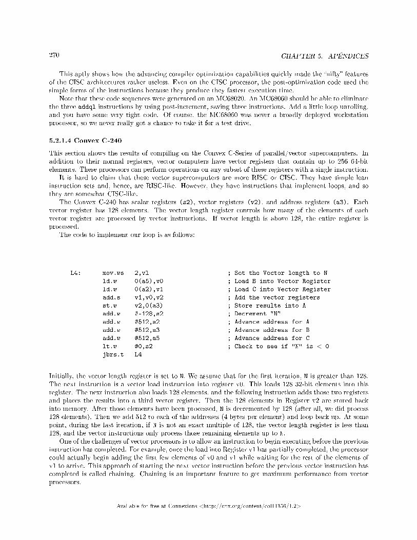
270 CHAPTER 5. APÉNDICES
This aptly shows how the advancing compiler optimization capabilities quickly made the �nifty� featuresof the CISC architectures rather useless. Even on the CISC processor, the post-optimization code used thesimple forms of the instructions because they produce they fastest execution time.
Note that these code sequences were generated on an MC68020. An MC68060 should be able to eliminatethe three addql instructions by using post-increment, saving three instructions. Add a little loop unrolling,and you have some very tight code. Of course, the MC68060 was never a broadly deployed workstationprocessor, so we never really got a chance to take it for a test drive.
5.2.1.4 Convex C-240
This section shows the results of compiling on the Convex C-Series of parallel/vector supercomputers. Inaddition to their normal registers, vector computers have vector registers that contain up to 256 64-bitelements. These processors can perform operations on any subset of these registers with a single instruction.
It is hard to claim that these vector supercomputers are more RISC or CISC. They have simple leaninstruction sets and, hence, are RISC-like. However, they have instructions that implement loops, and sothey are somewhat CISC-like.
The Convex C-240 has scalar registers (s2), vector registers (v2), and address registers (a3). Eachvector register has 128 elements. The vector length register controls how many of the elements of eachvector register are processed by vector instructions. If vector length is above 128, the entire register isprocessed.
The code to implement our loop is as follows:
L4: mov.ws 2,vl ; Set the Vector length to N
ld.w 0(a5),v0 ; Load B into Vector Register
ld.w 0(a2),v1 ; Load C into Vector Register
add.s v1,v0,v2 ; Add the vector registers
st.w v2,0(a3) ; Store results into A
add.w #-128,s2 ; Decrement "N"
add.w #512,a2 ; Advance address for A
add.w #512,a3 ; Advance address for B
add.w #512,a5 ; Advance address for C
lt.w #0,s2 ; Check to see if "N" is < 0
jbrs.t L4
Initially, the vector length register is set to N. We assume that for the �rst iteration, N is greater than 128.The next instruction is a vector load instruction into register v0. This loads 128 32-bit elements into thisregister. The next instruction also loads 128 elements, and the following instruction adds those two registersand places the results into a third vector register. Then the 128 elements in Register v2 are stored backinto memory. After those elements have been processed, N is decremented by 128 (after all, we did process128 elements). Then we add 512 to each of the addresses (4 bytes per element) and loop back up. At somepoint, during the last iteration, if N is not an exact multiple of 128, the vector length register is less than128, and the vector instructions only process those remaining elements up to N.
One of the challenges of vector processors is to allow an instruction to begin executing before the previousinstruction has completed. For example, once the load into Register v1 has partially completed, the processorcould actually begin adding the �rst few elements of v0 and v1 while waiting for the rest of the elements ofv1 to arrive. This approach of starting the next vector instruction before the previous vector instruction hascompleted is called chaining. Chaining is an important feature to get maximum performance from vectorprocessors.
Available for free at Connexions <http://cnx.org/content/col11356/1.2>
271
5.2.1.5 IBM RS-6000
The IBM RS-6000 is generally credited as the �rst RISC processor to have cracked the Linpack 100×100benchmark. The RS-6000 is characterized by strong �oating-point performance and excellent memory band-width among RISC workstations. The RS-6000 was the basis for IBM's scalable parallel processor: theIBM-SP1 and SP2.
When our example program is run on the RS-6000, we can see the use of a CISC- style instruction inthe middle of a RISC processor. The RS-6000 supports a branch- on-count instruction that combines thedecrement, test, and branch operations into a single instruction. Moreover, there is a special register (thecount register) that is part of the instruction fetch unit that stores the current value of the counter. Thefetch unit also has its own add unit to perform the decrements for this instruction.
These types of features creeping into RISC architectures are occuring because there is plenty of chipspace for them. If a wide range of programs can run faster with this type of instruction, it's often added.
The assembly code on the RS-6000 is:
ai r3,r3,-4 # Address of A(0)
ai r5,r5,-4 # Address of B(0)
ai r4,r4,-4 # Address of C(0)
bcr BO_IF_NOT,CR0_GT
mtspr CTR,r6 # Store in the Counter Register
__L18:
lfsu fp0,4(r4) # Pre Increment Load
lfsu fp1,4(r5) # Pre Increment Load
fa fp0,fp0,fp1
frsp fp0,fp0
stfsu fp0,4(r3) # Pre-increment Store
bc BO_dCTR_NZERO,CR0_LT,__L18 # Branch on Counter
The RS-6000 also supports a memory addressing mode that can add a value to its address register before usingthe address register. Interestingly, these two features (branch on count and pre-increment load) eliminateseveral instructions when compared to the more �pure� SPARC processor. The SPARC processor has 10instructions in the body of its loop, while the RS-6000 has 6 instructions.
The advantage of the RS-6000 in this particular loop may be less signi�cant if both processors weretwo-way superscalar. The instructions were eliminated on the RS-6000 were integer instructions. On atwo-way superscalar processor, those integer instructions may simply execute on the integer units while the�oating-point units are busy performing the �oating-point computations.
5.2.1.6 Conclusion
In this section, we have attempted to give you some understanding of the variety of assembly language thatis produced by compilers at di�erent optimization levels and on di�erent computer architectures. At somepoint during the tuning of your code, it can be quite instructive to take a look at the generated assemblylanguage to be sure that the compiler is not doing something really stupid that is slowing you down.
Please don't be tempted to rewrite portions in assembly language. Usually any problems can be solvedby cleaning up and streamlining your high-level source code and setting the proper compiler �ags.
It is interesting that very few people actually learn assembly language any more. Most folks �nd thatthe compiler is the best teacher of assembly language. By adding the appropriate option (often -S), thecompiler starts giving you lessons. I suggest that you don't print out all of the code. There are many pagesof useless variable declarations, etc. For these examples, I cut out all of that useless information. It is best
Available for free at Connexions <http://cnx.org/content/col11356/1.2>

272 CHAPTER 5. APÉNDICES
to view the assembly in an editor and only print out the portion that pertains to the particular loop you aretuning.
Available for free at Connexions <http://cnx.org/content/col11356/1.2>
INDEX 273
Index of Keywords and Terms
Keywords are listed by the section with that keyword (page numbers are in parentheses). Keywordsdo not necessarily appear in the text of the page. They are merely associated with that section. Ex.apples, � 1.1 (1) Terms are referenced by the page they appear on. Ex. apples, 1
A access patterns, � 2.4.7(115), � 2.4.9(118)accuracy, � 1.2.6(36)algebra, � 1.2.4(33), � 1.2.5(34)ambientes de paso de mensajes, � 4.2.2(220)ambiguous references, � 3.1.5(146)ancho de banda, � 1.1.7(20)antidependencies, � 3.1.4(141)análisis de �ujo de datos, � 2.1.5(54),� 3.1.2(130)análisis de per�l a tiempo de ejecución,� 2.1.5(54)análisis de punto �otante, � 2.1.5(54)análisis interprocedimental, � 2.1.5(54)apuntadores, � 2.1.3(49)apuntadores ambiguos, � 2.3.1(88)arquitectura de computadoras, � (3)arreglo IND, � 1.1.4(10)assembly language, � 5.2.1(262)assertions, � 3.3.3(183)associative transformation, � 1.2.4(33),� 1.2.5(34)automatic parallelization, � 3.3.2(176)
B back edge, � 3.1.3(139)backwards dependencies, � 3.1.4(141)banco de pruebas, � 2.2.1(63)barreras, � 2.3.1(88)benchmarks, � (3)bifurcaciones, � 2.3.3(93), � 2.3.4(94),� 2.4.4(108)bin, � 2.2.2(64)binary coded decimal, � 1.2.3(30)block, � 2.4.9(118)block reference, � 2.4.9(118)bloque básico, � 2.2.4(81)bloqueo, � 2.4.1(105)bloqueo de banco, � 1.1.7(20)bloques básicos, � 2.1.4(50)broadcast/gather, � 4.2.3(233)bucle, � 2.3.7(104)bucle condicional, � 2.3.7(104)bucle precondicionante, � 2.4.3(107)
bucles, � 2.2.3(70)bucles gruesos, � 2.4.4(108)bu�er de traducción de direcciones, � 1.1.6(17)buses, � 3.2.2(152)
C C++, � 2.1.3(49)cache, � 2.2.6(87)cache asociativa por conjuntos, � 1.1.5(13)cache coherency protocol, � 3.2.2(152)cache completamente asociativa, � 1.1.5(13)cache directamente mapeada, � 1.1.5(13)caches, � 1.1.2(8), � 1.1.4(10)caches grandes, � 1.1.7(20)caching, � 1.1.4(10)carga de trabajo, � 2.2.1(63)caza de apuntadores, � 1.1.4(10)ciclo, � 4.1.2(197)ciclos, � 2.3.4(94)CISC, � 5.1.2(245)coherency, � 3.2.2(152)compatibilidad de tamaño, � 4.1.4(203)compilador, � 2.1.1(47), � 2.1.3(49),� 2.1.4(50), � 2.1.6(55), � 2.1.7(62), � 2.1.8(62)compilador optimizador, � 2.1.1(47)compiladores, � 2.1.2(47), � 2.3.3(93)compiladores optimizadores, � 2.1.2(47)compiler, � 3.1.6(149), � 3.1.7(149),� 3.3.3(183)complex instruction set computer, � 5.1.2(245)conteo de iteraciones, � 2.4.4(108)conteo de operaciones, � 2.4.2(105)conversión de tipo de datos, � 2.3.5(99)copyback, � 3.2.2(152)critical sections, � 3.2.4(169)cronometraje, � 2.2.1(63), � 2.2.3(70),� 2.2.4(81), � 2.2.5(84), � 2.2.6(87), � 2.2.7(87)crossbars, � 3.2.2(152)cuádruplas, � 2.1.4(50)código muerte, � 2.1.6(55)cómputo de alto rendimiento, � (3),� 4.1.1(197), � 4.1.2(197), � 4.1.3(202),� 4.1.4(203), � 4.1.7(219)
Available for free at Connexions <http://cnx.org/content/col11356/1.2>
274 INDEX
D data �ow analysis, � 3.3.4(194)data placement, � 3.2.2(152)datos, � 3.1.2(130)datos en paralelo, � 4.1.2(197)datos paralelos, � 4.1.5(212)dependencia de control, � 3.1.2(130)dependencia de datos, � 3.1.2(130)dependencia del índice del ciclo, � 2.3.4(94)dependencies, � 3.1.3(139)dependency distance, � 3.1.5(146)descomposición de cálculos, � 4.1.5(212)descomposición de datos, � 4.1.5(212)descomposición de tareas, � 4.1.5(212)desenrollado de bucles, � 2.4.1(105),� 2.4.3(107)desenrollado de ciclos, � 2.4.4(108)desorden, � 2.3.5(99), � 2.3.6(104), � 2.3.7(104)desorden en un programa, � 2.3.6(104),� 2.3.7(104)distribución sobre procesadores, � 4.1.6(213)division by zero, � 1.2.10(43)DRAM, � 1.1.2(8), � 1.1.7(20)duración del ciclo de memoria, � 1.1.2(8)dynamic scheduling, � 3.3.3(183)
E E/S bloqueada, � 2.2.2(64)E/S de disco, � 2.2.5(84)eliminación de subexpresiones comunes,� 2.3.5(99)emerger, � 2.3.5(99)entubamiento, � 3.1.1(129)espacio de memoria compartida, � 2.2.2(64)estados de espera, � 1.1.2(8)estructuras de control HPF, � 4.1.6(213)estructuras intrínsecas HPF, � 4.1.6(213)etime, � 2.2.2(64), � 2.2.3(70), � 2.2.7(87)etiqueta, � 1.1.5(13)evitar cache, � 1.1.7(20)expresión constante, � 2.1.6(55)expresión invariante en el bucle, � 2.1.6(55)
F fallos de página, � 1.1.6(17), � 2.2.2(64),� 2.2.5(84)�xed point, � 1.2.3(30)�exibilidad del compilador, � 3.1.1(129)�oating-point number, � 1.2.2(29), � 1.2.3(30),� 1.2.9(42)�oating-point numbers, � 1.2.1(29),� 1.2.4(33), � 1.2.5(34), � 1.2.6(36), � 1.2.7(37),� 1.2.8(40), � 1.2.10(43), � 1.2.11(43),� 1.2.12(44), � 1.2.13(45)�otantes, � 2.3.5(99)
�ow dependencies, � 3.1.4(141)�ujo calorí�co, � 4.2.2(220)�ujo calórico, � 4.1.2(197), � 4.1.6(213)�ujo de control, � 3.1.2(130)�ujo término, � 4.1.4(203)fork-join programming, � 3.2.4(169)FORTRAN, � 1.1.2(8), � 1.2.11(43),� 2.1.2(47), � 2.1.3(49), � 2.1.6(55), � 2.3.2(89),� 2.3.5(99), � 2.4.3(107), � 2.4.5(111),� 2.4.7(115), � 2.4.9(118), � 2.4.11(125),� 2.4.12(125), � 3.1.5(146), � 3.1.7(149),� 3.2.3(157), � 3.3.1(176), � 3.3.3(183),� 4.1.1(197), � 4.1.3(202), � 4.1.7(219),� 4.2.1(220), � 4.2.3(233), � 5.2.1(262)FORTRAN 77, � 4.1.4(203), � 4.2.4(244)FORTRAN 90, � 4.1.4(203), � 4.1.5(212),� 4.1.6(213), � 4.2.4(244)FORTRAN de alto rendimiento, � 4.1.5(212),� 4.1.6(213)FORTRAN de alto rendimiento (HPF),� 4.1.7(219)
G gradual under�ow, � 1.2.9(42)grafo acíclico dirigido, � 3.1.2(130)granularidad, � 3.1.1(129)greatest common divisor, � 1.2.3(30)guard digits, � 1.2.6(36)
H heat �ow, � 4.2.3(233)High Performance Computing, � 5.1.1(245),� 5.1.2(245), � 5.1.3(247), � 5.1.4(256),� 5.1.5(258), � 5.1.6(259), � 5.1.7(261),� 5.1.8(261), � 5.2.1(262)HPC, � (3)
I IEEE, � 1.2.7(37)IEEE operations, � 1.2.8(40)inexact operation, � 1.2.10(43)inmersión, � 2.3.5(99)inner loop, � 2.4.5(111)instruction set, � 5.1.2(245)Intel 8088, � 5.2.1(262)intercambio de bucles, � 2.4.1(105)intercambios, � 2.2.2(64)interchange, � 2.4.8(118)interfaz de paso de mensajes, � 4.2.1(220)interprocedural analysis, � 3.3.3(183)invalid operations, � 1.2.10(43)invariantes, � 2.3.4(94)iteration scheduling, � 3.3.3(183)
J jerarquía de memoria, � 1.1.2(8)
Available for free at Connexions <http://cnx.org/content/col11356/1.2>
INDEX 275
L latencia, � 1.1.7(20)lenguaje, � 2.1.3(49), � 4.1.7(219)lenguaje intermedio, � 2.1.4(50)lenguajes paralelos, � 4.1.3(202)Ley de Amdahl, � 2.2.3(70)llamado a procedimientos, � 2.4.4(108)llamado a subrutinas, � 2.3.1(88), � 2.3.2(89)localidad de referencias espacial, � 1.1.4(10)localidad de referencias temporal, � 1.1.4(10)loop, � 3.1.3(139), � 3.3.5(195)loop interchange, � 2.4.6(114)loop nest, � 2.4.6(114)loop nests, � 2.4.5(111)loop omptimization, � 2.4.5(111)loop optimization, � 2.4.6(114), � 2.4.7(115),� 2.4.8(118), � 2.4.9(118), � 2.4.10(124)loop optimizations, � 2.4.11(125), � 2.4.12(125)loop unrolling, � 2.4.5(111)loop-carried dependencies, � 3.1.4(141)loops, � 2.4.11(125), � 2.4.12(125), � 3.1.4(141)
M macros, � 2.3.2(89)malloc, � 3.1.5(146)mantissa/exponent, � 1.2.3(30)mapeo, � 1.1.5(13)mapeo directo, � 1.1.5(13)medición de �ops, � 2.2.6(87)memoria, � (3), � 1.1.1(7), � 1.1.2(8),� 1.1.3(9), � 1.1.4(10), � 1.1.6(17), � 1.1.7(20),� 1.1.8(28), � 1.1.9(28)memoria de acceso aleatorio estática,� 1.1.4(10)memoria dinámica de acceso aleatorio,� 1.1.2(8)memoria estática de acceso aleatorio, � 1.1.2(8)memoria real libre, � 2.2.5(84)memoria virtual, � 1.1.6(17), � 2.2.5(84)memoria virtual activa, � 2.2.5(84)memory, � 2.4.7(115), � 2.4.9(118),� 2.4.10(124)message-passing environments, � 4.2.3(233),� 4.2.4(244)message-passing interface, � 4.2.3(233)mezcla de tipos, � 2.3.5(99)microprocesadores, � (3)mixed stride, � 2.4.9(118)modo kernel, � 2.2.2(64)modo usuario, � 2.2.2(64)move computation, � 2.4.6(114)multiprocessing, � 3.2.2(152)multiprocessors, � 3.2.1(151), � 3.2.3(157),
� 3.2.4(169), � 3.2.5(172), � 3.2.6(175),� 3.2.7(175), � 3.3.1(176), � 3.3.2(176),� 3.3.3(183), � 3.3.4(194), � 3.3.5(195)multithreading, � 3.2.3(157), � 3.2.4(169)máquina virtual paralela, � 4.2.1(220),� 4.2.2(220)
N niveles de optimización, � 2.1.5(54)no dependencies, � 3.3.3(183)no equivalence assertion, � 3.3.3(183)numerical analysis, � 1.2.1(29)
O optimización, � 2.1.3(49), � 2.1.6(55),� 2.1.7(62), � 2.1.8(62)optimización avanzada, � 2.1.5(54)optimización básica, � 2.1.5(54)optimización de bucles, � 2.4.3(107)optimización de bucles anidados, � 2.4.1(105)optimización de ciclos, � 2.4.2(105),� 2.4.4(108)optimización de referencias a memoria,� 2.4.1(105)optimizar, � 2.1.4(50)optimization, � 3.1.6(149), � 3.1.7(149),� 5.2.1(262)organización de la cache, � 1.1.5(13)out-of-core solutions, � 2.4.10(124)outer loop, � 2.4.5(111)output dependencies, � 3.1.4(141)over�ow to in�nity, � 1.2.10(43)
P paralelismo, � 2.3.6(104), � 2.3.7(104),� 3.1.1(129)paralelismo a nivel de hilos de ejecución,� 3.1.1(129)paralelismo a nivel de instrucciones,� 3.1.1(129)paralelo, � 4.1.4(203)parallel loops, � 3.3.3(183)parallel programming, � 3.3.5(195)parallel region, � 3.3.3(183)parallelism, � 3.1.4(141), � 3.1.5(146),� 3.1.6(149), � 3.1.7(149)parallelization, � 3.3.3(183)paso de mensajes, � 4.2.1(220)paso unitario, � 1.1.4(10)per�l plano, � 2.2.3(70)per�lado, � 2.2.1(63), � 2.2.2(64), � 2.2.3(70),� 2.2.4(81), � 2.2.5(84), � 2.2.6(87), � 2.2.7(87)per�lado de subrutinas, � 2.2.3(70)per�lador de bloques básicos, � 2.2.4(81)per�ladores, � 2.2.4(81)
Available for free at Connexions <http://cnx.org/content/col11356/1.2>
276 INDEX
permutation, � 3.1.5(146)permutation assertion, � 3.3.3(183)pixie, � 2.2.4(81)plegado de constantes, � 2.1.6(55)porcentaje de uso, � 2.2.2(64)Post-RISC, � 5.1.6(259)primitiva de asignación, � 4.1.4(203)producto de matrices, � 4.1.4(203)pro�ling, � 2.4.11(125), � 2.4.12(125)programación, � 4.1.6(213)programming, � 3.3.1(176), � 3.3.2(176),� 3.3.3(183), � 3.3.4(194), � 3.3.5(195)propagación, � 2.1.6(55)protocolos de datagramas de usuario,� 4.2.2(220)pruebas exageradas, � 2.3.1(88)PVM, � 4.2.1(220), � 4.2.2(220)páginas, � 1.1.6(17)
R racionalizar, � 2.3.3(93)rational numbers, � 1.2.2(29), � 1.2.3(30)reality, � 1.2.2(29)reducción de resistencia, � 2.1.6(55)reduced instruction set computer, � 5.1.5(258),� 5.1.6(259)reduced instruction set computing,� 5.1.3(247), � 5.1.4(256)reduction operations, � 3.3.2(176)reductions, � 3.1.4(141)referencias indirectas a memoria, � 2.3.1(88)registros, � 1.1.2(8), � 1.1.3(9)relation assertion, � 3.3.3(183)renombramiento de variables, � 2.1.6(55)representation, � 1.2.3(30)RISC, � 2.1.7(62), � 2.1.8(62), � 5.1.3(247),� 5.1.4(256), � 5.1.5(258)
S scale parallel computing, � 3.2.3(157)secciones de arreglos, � 4.1.4(203)sentencia función, � 2.3.2(89)shared-memory, � 3.2.1(151), � 3.2.3(157),� 3.2.4(169), � 3.2.5(172), � 3.2.6(175),� 3.2.7(175), � 3.3.1(176), � 3.3.2(176),� 3.3.3(183), � 3.3.4(194), � 3.3.5(195)signi�cand, � 1.2.8(40)simpli�cación de variables de inducción,
� 2.1.6(55)sin optimización, � 2.1.5(54)snooping, � 3.2.2(152)software, � 3.2.3(157)soluciones fuera del núcleo, � 2.4.1(105)soporte del lenguaje, � 4.1.1(197), � 4.1.6(213)SPARC, � 5.2.1(262)speedup, � 3.3.2(176)SRAM, � 1.1.2(8), � 1.1.4(10), � 1.1.7(20)stride, � 2.4.7(115)subexpresiones comunes, � 2.1.6(55)subrutinas en línea, � 2.3.2(89)superescalar, � 3.1.1(129)synchronization, � 3.2.4(169)
T tablas de páginas, � 1.1.6(17)tamaño, � 2.2.5(84)techniques, � 3.2.4(169)thrashing, � 1.1.5(13)thread, � 3.2.3(157)thread private, � 3.2.3(157)thread-local variables, � 3.2.3(157)tiempo, � 2.2.2(64)tiempo de acceso a memoria, � 1.1.2(8)tiempo de CPU, � 2.2.2(64)tiempo de sistema, � 2.2.2(64)tiempo de usuario, � 2.2.2(64)tiempo utilizado, � 2.2.2(64)time-based simulation, � 3.2.4(169)timing, � 2.2.2(64), � 2.4.11(125), � 2.4.12(125)trip count assertion, � 3.3.3(183)técnicas de a�nación, � 2.3.6(104), � 2.3.7(104)
U uniform memory access, � 3.2.1(151)user=space thread context switch, � 3.2.3(157)uso promedio de memoria, � 2.2.2(64)
V valoración de arreglos, � 4.1.4(203)variables de inducción, � 2.1.6(55)velocidad de CPU, � 1.1.1(7)
W write-through policy, � 3.2.2(152)writeback, � 3.2.2(152)
á área de intercambio, � 2.2.5(84)
Available for free at Connexions <http://cnx.org/content/col11356/1.2>
ATTRIBUTIONS 277
Attributions
Collection: Cómputo de Alto RendimientoEdited by: José Enrique Alvarez EstradaURL: http://cnx.org/content/col11356/1.2/License: http://creativecommons.org/licenses/by/3.0/
Module: "1.0 Introducción a la Edición de Connexions"By: José Enrique Alvarez EstradaURL: http://cnx.org/content/m38315/1.1/Pages: 1-2Copyright: José Enrique Alvarez EstradaLicense: http://creativecommons.org/licenses/by/3.0/Based on: 1.0 Introduction to the Connexions EditionBy: Charles SeveranceURL: http://cnx.org/content/m32709/1.1/
Module: "Introducción al Cómputo de Alto Rendimiento"By: José Enrique Alvarez EstradaURL: http://cnx.org/content/m37223/1.1/Pages: 3-6Copyright: José Enrique Alvarez EstradaLicense: http://creativecommons.org/licenses/by/3.0/Based on: Introduction to High Performance ComputingBy: Charles Severance, Kevin DowdURL: http://cnx.org/content/m32676/1.3/
Module: "Introducción"By: José Enrique Alvarez EstradaURL: http://cnx.org/content/m37222/1.1/Pages: 7-8Copyright: José Enrique Alvarez EstradaLicense: http://creativecommons.org/licenses/by/3.0/Based on: Memory - IntroductionBy: Charles Severance, Kevin DowdURL: http://cnx.org/content/m32733/1.3/
Module: "Tecnologías de Memoria"By: José Enrique Alvarez EstradaURL: http://cnx.org/content/m37229/1.1/Pages: 8-9Copyright: José Enrique Alvarez EstradaLicense: http://creativecommons.org/licenses/by/3.0/Based on: Memory - Memory TechnologyBy: Charles Severance, Kevin DowdURL: http://cnx.org/content/m32716/1.3/
Available for free at Connexions <http://cnx.org/content/col11356/1.2>

278 ATTRIBUTIONS
Module: "Registros"By: José Enrique Alvarez EstradaURL: http://cnx.org/content/m37228/1.1/Pages: 9-10Copyright: José Enrique Alvarez EstradaLicense: http://creativecommons.org/licenses/by/3.0/Based on: Memory - RegistersBy: Charles Severance, Kevin DowdURL: http://cnx.org/content/m32681/1.3/
Module: "Caches"By: José Enrique Alvarez EstradaURL: http://cnx.org/content/m37220/1.2/Pages: 10-13Copyright: José Enrique Alvarez EstradaLicense: http://creativecommons.org/licenses/by/3.0/Based on: Memory - CachesBy: Charles Severance, Kevin DowdURL: http://cnx.org/content/m32725/1.3/
Module: "Organización de la Cache"By: José Enrique Alvarez EstradaURL: http://cnx.org/content/m37227/1.2/Pages: 13-17Copyright: José Enrique Alvarez EstradaLicense: http://creativecommons.org/licenses/by/3.0/Based on: Memory - Cache OrganizationBy: Charles Severance, Kevin DowdURL: http://cnx.org/content/m32722/1.3/
Module: "Memoria Virtual"By: José Enrique Alvarez EstradaURL: http://cnx.org/content/m37225/1.1/Pages: 17-20Copyright: José Enrique Alvarez EstradaLicense: http://creativecommons.org/licenses/by/3.0/Based on: Memory - Virtual MemoryBy: Charles Severance, Kevin DowdURL: http://cnx.org/content/m32728/1.3/
Module: "Mejorando el Rendimiento de la Memoria"By: José Enrique Alvarez EstradaURL: http://cnx.org/content/m37224/1.1/Pages: 20-28Copyright: José Enrique Alvarez EstradaLicense: http://creativecommons.org/licenses/by/3.0/Based on: Memory - Improving Memory PerformanceBy: Charles Severance, Kevin DowdURL: http://cnx.org/content/m32736/1.3/
Available for free at Connexions <http://cnx.org/content/col11356/1.2>

ATTRIBUTIONS 279
Module: "Notas de Cierre"By: José Enrique Alvarez EstradaURL: http://cnx.org/content/m37226/1.1/Page: 28Copyright: José Enrique Alvarez EstradaLicense: http://creativecommons.org/licenses/by/3.0/Based on: Memory - Closing NotesBy: Charles Severance, Kevin DowdURL: http://cnx.org/content/m32690/1.3/
Module: "Ejercicios"By: José Enrique Alvarez EstradaURL: http://cnx.org/content/m37221/1.1/Pages: 28-29Copyright: José Enrique Alvarez EstradaLicense: http://creativecommons.org/licenses/by/3.0/Based on: Memory - ExercisesBy: Charles Severance, Kevin DowdURL: http://cnx.org/content/m32698/1.3/
Module: "Floating-Point Numbers - Introduction"Used here as: "Introduction"By: Charles Severance, Kevin DowdURL: http://cnx.org/content/m32739/1.3/Page: 29Copyright: Charles Severance, Kevin DowdLicense: http://creativecommons.org/licenses/by/3.0/
Module: "Floating-Point Numbers - Reality"Used here as: "Reality"By: Charles Severance, Kevin DowdURL: http://cnx.org/content/m32741/1.3/Pages: 29-30Copyright: Charles Severance, Kevin DowdLicense: http://creativecommons.org/licenses/by/3.0/
Module: "Floating-Point Numbers - Representation"Used here as: "Representation"By: Charles Severance, Kevin DowdURL: http://cnx.org/content/m32772/1.3/Pages: 30-33Copyright: Charles Severance, Kevin DowdLicense: http://creativecommons.org/licenses/by/3.0/
Module: "Floating-Point Numbers - E�ects of Floating-Point Representation"Used here as: "E�ects of Floating-Point Representation"By: Charles Severance, Kevin DowdURL: http://cnx.org/content/m32755/1.3/Pages: 33-34Copyright: Charles Severance, Kevin DowdLicense: http://creativecommons.org/licenses/by/3.0/
Available for free at Connexions <http://cnx.org/content/col11356/1.2>

280 ATTRIBUTIONS
Module: "Floating-Point Numbers - More Algebra That Doesn't Work"Used here as: "More Algebra That Doesn't Work"By: Charles Severance, Kevin DowdURL: http://cnx.org/content/m32754/1.3/Pages: 34-36Copyright: Charles Severance, Kevin DowdLicense: http://creativecommons.org/licenses/by/3.0/
Module: "Floating-Point Numbers - Improving Accuracy Using Guard Digits"Used here as: "Improving Accuracy Using Guard Digits"By: Charles Severance, Kevin DowdURL: http://cnx.org/content/m32744/1.3/Pages: 36-37Copyright: Charles Severance, Kevin DowdLicense: http://creativecommons.org/licenses/by/3.0/
Module: "Floating-Point Numbers - History of IEEE Floating-Point Format"Used here as: "History of IEEE Floating-Point Format"By: Charles Severance, Kevin DowdURL: http://cnx.org/content/m32770/1.3/Pages: 37-40Copyright: Charles Severance, Kevin DowdLicense: http://creativecommons.org/licenses/by/3.0/
Module: "Floating-Point Numbers - IEEE Operations"Used here as: "IEEE Operations"By: Charles Severance, Kevin DowdURL: http://cnx.org/content/m32756/1.3/Pages: 40-42Copyright: Charles Severance, Kevin DowdLicense: http://creativecommons.org/licenses/by/3.0/
Module: "Floating-Point Numbers - Special Values"Used here as: "Special Values"By: Charles Severance, Kevin DowdURL: http://cnx.org/content/m32758/1.3/Pages: 42-43Copyright: Charles Severance, Kevin DowdLicense: http://creativecommons.org/licenses/by/3.0/
Module: "Floating-Point Numbers - Exceptions and Traps"Used here as: "Exceptions and Traps"By: Charles Severance, Kevin DowdURL: http://cnx.org/content/m32760/1.3/Page: 43Copyright: Charles Severance, Kevin DowdLicense: http://creativecommons.org/licenses/by/3.0/
Available for free at Connexions <http://cnx.org/content/col11356/1.2>

ATTRIBUTIONS 281
Module: "Floating-Point Numbers - Compiler Issues"Used here as: "Compiler Issues"By: Charles Severance, Kevin DowdURL: http://cnx.org/content/m32762/1.3/Pages: 43-44Copyright: Charles Severance, Kevin DowdLicense: http://creativecommons.org/licenses/by/3.0/
Module: "Floating-Point Numbers - Closing Notes"Used here as: "Closing Notes"By: Charles Severance, Kevin DowdURL: http://cnx.org/content/m32768/1.3/Pages: 44-45Copyright: Charles Severance, Kevin DowdLicense: http://creativecommons.org/licenses/by/3.0/
Module: "Floating-Point Numbers - Exercises"Used here as: "Exercises"By: Charles Severance, Kevin DowdURL: http://cnx.org/content/m32765/1.3/Page: 45Copyright: Charles Severance, Kevin DowdLicense: http://creativecommons.org/licenses/by/3.0/
Module: "Qué Hace un Compilador - Introducción"By: José Enrique Alvarez EstradaURL: http://cnx.org/content/m38387/1.2/Page: 47Copyright: José Enrique Alvarez EstradaLicense: http://creativecommons.org/licenses/by/3.0/Based on: What a Compiler Does - IntroductionBy: Charles Severance, Kevin DowdURL: http://cnx.org/content/m33690/1.3/
Module: "Qué Hace un Compilador - Historia de los Compiladores"By: José Enrique Alvarez EstradaURL: http://cnx.org/content/m38391/1.2/Pages: 47-49Copyright: José Enrique Alvarez EstradaLicense: http://creativecommons.org/licenses/by/3.0/Based on: What a Compiler Does - History of CompilersBy: Charles Severance, Kevin DowdURL: http://cnx.org/content/m33686/1.3/
Module: "Qué Hace un Compilador - Cuál Lenguaje Optimizar"By: José Enrique Alvarez EstradaURL: http://cnx.org/content/m38392/1.2/Pages: 49-50Copyright: José Enrique Alvarez EstradaLicense: http://creativecommons.org/licenses/by/3.0/Based on: What a Compiler Does - Which Language To OptimizeBy: Charles Severance, Kevin DowdURL: http://cnx.org/content/m33687/1.3/
Available for free at Connexions <http://cnx.org/content/col11356/1.2>

282 ATTRIBUTIONS
Module: "Qué Hace un Compilador - Visita Guiada al Optimizador de Código"By: José Enrique Alvarez EstradaURL: http://cnx.org/content/m38394/1.1/Pages: 50-54Copyright: José Enrique Alvarez EstradaLicense: http://creativecommons.org/licenses/by/3.0/Based on: What a Compiler Does - Optimizing Compiler TourBy: Charles Severance, Kevin DowdURL: http://cnx.org/content/m33694/1.3/
Module: "Qué Hace un Compilador - Niveles de Optimización"By: José Enrique Alvarez EstradaURL: http://cnx.org/content/m38395/1.1/Pages: 54-55Copyright: José Enrique Alvarez EstradaLicense: http://creativecommons.org/licenses/by/3.0/Based on: What a Compiler Does - Optimization LevelsBy: Charles Severance, Kevin DowdURL: http://cnx.org/content/m33692/1.3/
Module: "Qué Hace un Compilador - Optimizaciones Clásicas"By: José Enrique Alvarez EstradaURL: http://cnx.org/content/m38400/1.1/Pages: 55-62Copyright: José Enrique Alvarez EstradaLicense: http://creativecommons.org/licenses/by/3.0/Based on: What a Compiler Does - Classical OptimizationsBy: Charles Severance, Kevin DowdURL: http://cnx.org/content/m33696/1.3/
Module: "Qué Hace un Compilador - Notas de Cierre"By: José Enrique Alvarez EstradaURL: http://cnx.org/content/m38402/1.1/Page: 62Copyright: José Enrique Alvarez EstradaLicense: http://creativecommons.org/licenses/by/3.0/Based on: What a Compiler Does - Closing NotesBy: Charles Severance, Kevin DowdURL: http://cnx.org/content/m33699/1.3/
Module: "Qué Hace un Compilador - Ejercicios"By: José Enrique Alvarez EstradaURL: http://cnx.org/content/m38401/1.1/Pages: 62-63Copyright: José Enrique Alvarez EstradaLicense: http://creativecommons.org/licenses/by/3.0/Based on: What a Compiler Does - ExercisesBy: Charles Severance, Kevin DowdURL: http://cnx.org/content/m33700/1.3/
Available for free at Connexions <http://cnx.org/content/col11356/1.2>

ATTRIBUTIONS 283
Module: "Cronometraje y Per�lado - Introducción"By: José Enrique Alvarez EstradaURL: http://cnx.org/content/m38404/1.2/Pages: 63-64Copyright: José Enrique Alvarez EstradaLicense: http://creativecommons.org/licenses/by/3.0/Based on: Timing and Pro�ling - IntroductionBy: Charles Severance, Kevin DowdURL: http://cnx.org/content/m33704/1.3/
Module: "Cronometraje y Per�lado - Cronometraje"By: José Enrique Alvarez EstradaURL: http://cnx.org/content/m38409/1.2/Pages: 64-70Copyright: José Enrique Alvarez EstradaLicense: http://creativecommons.org/licenses/by/3.0/Based on: Timing and Pro�ling - TimingBy: Charles Severance, Kevin DowdURL: http://cnx.org/content/m33706/1.3/
Module: "Cronometraje y Per�lado - Per�lado de Subrutinas"By: José Enrique Alvarez EstradaURL: http://cnx.org/content/m38416/1.2/Pages: 70-81Copyright: José Enrique Alvarez EstradaLicense: http://creativecommons.org/licenses/by/3.0/Based on: Timing and Pro�ling - Subroutine Pro�lingBy: Charles Severance, Kevin DowdURL: http://cnx.org/content/m33713/1.3/
Module: "Cronometraje y Per�lado - Per�ladores de Bloques Básicos"By: José Enrique Alvarez EstradaURL: http://cnx.org/content/m38419/1.1/Pages: 81-84Copyright: José Enrique Alvarez EstradaLicense: http://creativecommons.org/licenses/by/3.0/Based on: Timing and Pro�ling - Basic Block Pro�lersBy: Charles Severance, Kevin DowdURL: http://cnx.org/content/m33710/1.3/
Module: "Cronometraje y Per�lado - Memoria Virtual"By: José Enrique Alvarez EstradaURL: http://cnx.org/content/m38424/1.1/Pages: 84-87Copyright: José Enrique Alvarez EstradaLicense: http://creativecommons.org/licenses/by/3.0/Based on: Timing and Pro�ling - Virtual MemoryBy: Charles Severance, Kevin DowdURL: http://cnx.org/content/m33712/1.3/
Available for free at Connexions <http://cnx.org/content/col11356/1.2>

284 ATTRIBUTIONS
Module: "Cronometraje y Per�lado - Notas de Cierre"By: José Enrique Alvarez EstradaURL: http://cnx.org/content/m38425/1.1/Page: 87Copyright: José Enrique Alvarez EstradaLicense: http://creativecommons.org/licenses/by/3.0/Based on: Timing and Pro�ling - Closing NotesBy: Charles Severance, Kevin DowdURL: http://cnx.org/content/m33714/1.3/
Module: "Cronometraje y Per�lado - Ejercicios"By: José Enrique Alvarez EstradaURL: http://cnx.org/content/m38426/1.1/Pages: 87-88Copyright: José Enrique Alvarez EstradaLicense: http://creativecommons.org/licenses/by/3.0/Based on: Timing and Pro�ling - ExercisesBy: Charles Severance, Kevin DowdURL: http://cnx.org/content/m33718/1.3/
Module: "Eliminando el Desorden - Introducción"By: José Enrique Alvarez EstradaURL: http://cnx.org/content/m38428/1.3/Pages: 88-89Copyright: José Enrique Alvarez EstradaLicense: http://creativecommons.org/licenses/by/3.0/Based on: Eliminating Clutter - IntroductionBy: Charles Severance, Kevin DowdURL: http://cnx.org/content/m33720/1.3/
Module: "Eliminando el Desorden - Llamado a Subrutinas"By: José Enrique Alvarez EstradaURL: http://cnx.org/content/m38429/1.2/Pages: 89-93Copyright: José Enrique Alvarez EstradaLicense: http://creativecommons.org/licenses/by/3.0/Based on: Eliminating Clutter - Subroutine CallsBy: Charles Severance, Kevin DowdURL: http://cnx.org/content/m33721/1.3/
Module: "Eliminando el Desorden - Bifurcaciones"By: José Enrique Alvarez EstradaURL: http://cnx.org/content/m38430/1.2/Pages: 93-94Copyright: José Enrique Alvarez EstradaLicense: http://creativecommons.org/licenses/by/3.0/Based on: Eliminating Clutter - BranchesBy: Charles Severance, Kevin DowdURL: http://cnx.org/content/m33722/1.3/
Available for free at Connexions <http://cnx.org/content/col11356/1.2>

ATTRIBUTIONS 285
Module: "Eliminando el Desorden - Bifurcaciones en Ciclos"Used here as: "Eliminando el Desorden - Bifurcaciones con Ciclos"By: José Enrique Alvarez EstradaURL: http://cnx.org/content/m38439/1.2/Pages: 94-99Copyright: José Enrique Alvarez EstradaLicense: http://creativecommons.org/licenses/by/3.0/Based on: Eliminating Clutter - Branches With LoopsBy: Charles Severance, Kevin DowdURL: http://cnx.org/content/m33723/1.3/
Module: "Eliminando el Desorden - Otras Formas de Desorden"By: José Enrique Alvarez EstradaURL: http://cnx.org/content/m38441/1.2/Pages: 99-104Copyright: José Enrique Alvarez EstradaLicense: http://creativecommons.org/licenses/by/3.0/Based on: Eliminating Clutter - Other ClutterBy: Charles Severance, Kevin DowdURL: http://cnx.org/content/m33724/1.3/
Module: "Eliminando el Desorden - Notas de Cierre"By: José Enrique Alvarez EstradaURL: http://cnx.org/content/m38442/1.2/Page: 104Copyright: José Enrique Alvarez EstradaLicense: http://creativecommons.org/licenses/by/3.0/Based on: Eliminating Clutter - Closing NotesBy: Charles Severance, Kevin DowdURL: http://cnx.org/content/m33725/1.3/
Module: "Eliminando el Desorden - Ejercicios"By: José Enrique Alvarez EstradaURL: http://cnx.org/content/m38443/1.2/Pages: 104-105Copyright: José Enrique Alvarez EstradaLicense: http://creativecommons.org/licenses/by/3.0/Based on: Eliminating Clutter - ExercisesBy: Charles Severance, Kevin DowdURL: http://cnx.org/content/m33727/1.3/
Module: "Optimización de Ciclos - Introducción"By: José Enrique Alvarez EstradaURL: http://cnx.org/content/m38445/1.2/Page: 105Copyright: José Enrique Alvarez EstradaLicense: http://creativecommons.org/licenses/by/3.0/Based on: Loop Optimizations - IntroductionBy: Charles Severance, Kevin DowdURL: http://cnx.org/content/m33728/1.3/
Available for free at Connexions <http://cnx.org/content/col11356/1.2>

286 ATTRIBUTIONS
Module: "Optimización de Ciclos - Conteo de Operaciones"By: José Enrique Alvarez EstradaURL: http://cnx.org/content/m38446/1.1/Pages: 105-107Copyright: José Enrique Alvarez EstradaLicense: http://creativecommons.org/licenses/by/3.0/Based on: Loop Optimizations - Operation CountingBy: Charles Severance, Kevin DowdURL: http://cnx.org/content/m33729/1.3/
Module: "Optimización de Ciclos - Desenrollado Básico de Ciclos"By: José Enrique Alvarez EstradaURL: http://cnx.org/content/m38449/1.2/Pages: 107-108Copyright: José Enrique Alvarez EstradaLicense: http://creativecommons.org/licenses/by/3.0/Based on: Loop Optimizations - Basic Loop UnrollingBy: Charles Severance, Kevin DowdURL: http://cnx.org/content/m33732/1.3/
Module: "Optimización de Ciclos - Cali�cando a los Candidatos para el Desenrollado de Ciclos"By: José Enrique Alvarez EstradaURL: http://cnx.org/content/m38486/1.2/Pages: 108-111Copyright: José Enrique Alvarez EstradaLicense: http://creativecommons.org/licenses/by/3.0/Based on: Loop Optimizations - Qualifying Candidates for Loop UnrollingBy: Charles Severance, Kevin DowdURL: http://cnx.org/content/m33733/1.3/
Module: "Loop Optimizations - Nested Loops"Used here as: "Nested Loops"By: Charles Severance, Kevin DowdURL: http://cnx.org/content/m33734/1.3/Pages: 111-114Copyright: Charles Severance, Kevin DowdLicense: http://creativecommons.org/licenses/by/3.0/
Module: "Loop Optimizations - Loop Interchange"Used here as: "Loop Interchange"By: Charles Severance, Kevin DowdURL: http://cnx.org/content/m33736/1.3/Pages: 114-115Copyright: Charles Severance, Kevin DowdLicense: http://creativecommons.org/licenses/by/3.0/
Module: "Loop Optimizations - Memory Access Patterns"Used here as: "Memory Access Patterns"By: Charles Severance, Kevin DowdURL: http://cnx.org/content/m33738/1.3/Pages: 115-118Copyright: Charles Severance, Kevin DowdLicense: http://creativecommons.org/licenses/by/3.0/
Available for free at Connexions <http://cnx.org/content/col11356/1.2>
ATTRIBUTIONS 287
Module: "Loop Optimizations - When Interchange Won't Work"Used here as: "When Interchange Won't Work"By: Charles Severance, Kevin DowdURL: http://cnx.org/content/m33741/1.3/Page: 118Copyright: Charles Severance, Kevin DowdLicense: http://creativecommons.org/licenses/by/3.0/
Module: "Loop Optimizations - Blocking to Ease Memory Access Patterns"Used here as: "Blocking to Ease Memory Access Patterns"By: Charles Severance, Kevin DowdURL: http://cnx.org/content/m33756/1.3/Pages: 118-124Copyright: Charles Severance, Kevin DowdLicense: http://creativecommons.org/licenses/by/3.0/
Module: "Loop Optimizations - Programs That Require More Memory Than You Have"Used here as: "Programs That Require More Memory Than You Have"By: Charles Severance, Kevin DowdURL: http://cnx.org/content/m33770/1.3/Pages: 124-125Copyright: Charles Severance, Kevin DowdLicense: http://creativecommons.org/licenses/by/3.0/
Module: "Loop Optimizations - Closing Notes"Used here as: "Closing Notes"By: Charles Severance, Kevin DowdURL: http://cnx.org/content/m33773/1.3/Page: 125Copyright: Charles Severance, Kevin DowdLicense: http://creativecommons.org/licenses/by/3.0/
Module: "Loop Optimizations - Exercises"Used here as: "Exercises"By: Charles Severance, Kevin DowdURL: http://cnx.org/content/m33777/1.3/Pages: 125-127Copyright: Charles Severance, Kevin DowdLicense: http://creativecommons.org/licenses/by/3.0/
Module: "Entendiendo el Paralelismo - Introducción"By: José Enrique Alvarez EstradaURL: http://cnx.org/content/m37327/1.1/Pages: 129-130Copyright: José Enrique Alvarez EstradaLicense: http://creativecommons.org/licenses/by/3.0/Based on: Understanding Parallelism - IntroductionBy: Charles Severance, Kevin DowdURL: http://cnx.org/content/m32775/1.3/
Available for free at Connexions <http://cnx.org/content/col11356/1.2>

288 ATTRIBUTIONS
Module: "Entendiendo el Paralelismo - Dependencias"By: José Enrique Alvarez EstradaURL: http://cnx.org/content/m37401/1.1/Pages: 130-139Copyright: José Enrique Alvarez EstradaLicense: http://creativecommons.org/licenses/by/3.0/Based on: Understanding Parallelism - DependenciesBy: Charles Severance, Kevin DowdURL: http://cnx.org/content/m32777/1.3/
Module: "Understanding Parallelism - Loops"Used here as: "Loops"By: Charles Severance, Kevin DowdURL: http://cnx.org/content/m32784/1.3/Pages: 139-141Copyright: Charles Severance, Kevin DowdLicense: http://creativecommons.org/licenses/by/3.0/
Module: "Understanding Parallelism - Loop-Carried Dependencies"Used here as: "Loop-Carried Dependencies "By: Charles Severance, Kevin DowdURL: http://cnx.org/content/m32782/1.3/Pages: 141-146Copyright: Charles Severance, Kevin DowdLicense: http://creativecommons.org/licenses/by/3.0/
Module: "Understanding Parallelism - Ambiguous References"Used here as: "Ambiguous References"By: Charles Severance, Kevin DowdURL: http://cnx.org/content/m32788/1.3/Pages: 146-149Copyright: Charles Severance, Kevin DowdLicense: http://creativecommons.org/licenses/by/3.0/
Module: "Understanding Parallelism - Closing Notes"Used here as: "Closing Notes"By: Charles Severance, Kevin DowdURL: http://cnx.org/content/m32789/1.3/Page: 149Copyright: Charles Severance, Kevin DowdLicense: http://creativecommons.org/licenses/by/3.0/
Module: "Understanding Parallelism - Exercises"Used here as: "Exercises"By: Charles Severance, Kevin DowdURL: http://cnx.org/content/m32792/1.3/Pages: 149-151Copyright: Charles Severance, Kevin DowdLicense: http://creativecommons.org/licenses/by/3.0/
Available for free at Connexions <http://cnx.org/content/col11356/1.2>
ATTRIBUTIONS 289
Module: "Shared-Memory Multiprocessors - Introduction"Used here as: "Introduction"By: Charles Severance, Kevin DowdURL: http://cnx.org/content/m32797/1.3/Pages: 151-152Copyright: Charles Severance, Kevin DowdLicense: http://creativecommons.org/licenses/by/3.0/
Module: "Shared-Memory Multiprocessors - Symmetric Multiprocessing Hardware"Used here as: "Symmetric Multiprocessing Hardware"By: Charles Severance, Kevin DowdURL: http://cnx.org/content/m32794/1.3/Pages: 152-157Copyright: Charles Severance, Kevin DowdLicense: http://creativecommons.org/licenses/by/3.0/
Module: "Shared-Memory Multiprocessors - Multiprocessor Software Concepts"Used here as: "Multiprocessor Software Concepts "By: Charles Severance, Kevin DowdURL: http://cnx.org/content/m32800/1.3/Pages: 157-169Copyright: Charles Severance, Kevin DowdLicense: http://creativecommons.org/licenses/by/3.0/
Module: "Shared-Memory Multiprocessors - Techniques for Multithreaded Programs"Used here as: "Techniques for Multithreaded Programs"By: Charles Severance, Kevin DowdURL: http://cnx.org/content/m32802/1.3/Pages: 169-172Copyright: Charles Severance, Kevin DowdLicense: http://creativecommons.org/licenses/by/3.0/
Module: "Shared-Memory Multiprocessors - A Real Example"Used here as: "A Real Example "By: Charles Severance, Kevin DowdURL: http://cnx.org/content/m32804/1.3/Pages: 172-175Copyright: Charles Severance, Kevin DowdLicense: http://creativecommons.org/licenses/by/3.0/
Module: "Shared-Memory Multiprocessors - Closing Notes"Used here as: "Closing Notes"By: Charles Severance, Kevin DowdURL: http://cnx.org/content/m32807/1.3/Page: 175Copyright: Charles Severance, Kevin DowdLicense: http://creativecommons.org/licenses/by/3.0/
Available for free at Connexions <http://cnx.org/content/col11356/1.2>
290 ATTRIBUTIONS
Module: "Shared-Memory Multiprocessors - Exercises"Used here as: "Exercises"By: Charles Severance, Kevin DowdURL: http://cnx.org/content/m32810/1.3/Pages: 175-176Copyright: Charles Severance, Kevin DowdLicense: http://creativecommons.org/licenses/by/3.0/
Module: "Programming Shared-Memory Multiprocessors - Introduction"Used here as: " Introduction"By: Charles Severance, Kevin DowdURL: http://cnx.org/content/m32812/1.3/Page: 176Copyright: Charles Severance, Kevin DowdLicense: http://creativecommons.org/licenses/by/3.0/
Module: "Programming Shared-Memory Multiprocessors - Automatic Parallelization"Used here as: "Automatic Parallelization"By: Charles Severance, Kevin DowdURL: http://cnx.org/content/m32821/1.3/Pages: 176-183Copyright: Charles Severance, Kevin DowdLicense: http://creativecommons.org/licenses/by/3.0/
Module: "Programming Shared-Memory Multiprocessors - Assisting the Compiler"Used here as: "Assisting the Compiler"By: Charles Severance, Kevin DowdURL: http://cnx.org/content/m32814/1.3/Pages: 183-194Copyright: Charles Severance, Kevin DowdLicense: http://creativecommons.org/licenses/by/3.0/
Module: "Programming Shared-Memory Multiprocessors - Closing Notes"Used here as: "Closing Notes"By: Charles Severance, Kevin DowdURL: http://cnx.org/content/m32820/1.3/Pages: 194-195Copyright: Charles Severance, Kevin DowdLicense: http://creativecommons.org/licenses/by/3.0/
Module: "Programming Shared-Memory Multiprocessors - Exercises"Used here as: "Exercises"By: Charles Severance, Kevin DowdURL: http://cnx.org/content/m32819/1.3/Pages: 195-196Copyright: Charles Severance, Kevin DowdLicense: http://creativecommons.org/licenses/by/3.0/
Available for free at Connexions <http://cnx.org/content/col11356/1.2>

ATTRIBUTIONS 291
Module: "Soporte del Lenguaje para Mejorar el Rendimiento - Introducción"By: José Enrique Alvarez EstradaURL: http://cnx.org/content/m38316/1.1/Page: 197Copyright: José Enrique Alvarez EstradaLicense: http://creativecommons.org/licenses/by/3.0/Based on: Language Support for Performance - IntroductionBy: Charles Severance, Kevin DowdURL: http://cnx.org/content/m33744/1.3/
Module: "Soporte del Lenguaje para Mejorar el Rendimiento - Problema de Datos en Paralelo: FlujoCalórico"By: José Enrique Alvarez EstradaURL: http://cnx.org/content/m38317/1.1/Pages: 197-202Copyright: José Enrique Alvarez EstradaLicense: http://creativecommons.org/licenses/by/3.0/Based on: Language Support for Performance - Data-Parallel Problem: Heat FlowBy: Charles Severance, Kevin DowdURL: http://cnx.org/content/m33751/1.3/
Module: "Soporte del Lenguaje para Mejorar el Rendimiento - Lenguajes Explícitamente Paralelos"By: José Enrique Alvarez EstradaURL: http://cnx.org/content/m38318/1.1/Pages: 202-203Copyright: José Enrique Alvarez EstradaLicense: http://creativecommons.org/licenses/by/3.0/Based on: Language Support for Performance - Explicity Parallel LanguagesBy: Charles Severance, Kevin DowdURL: http://cnx.org/content/m33754/1.3/
Module: "Soporte del Lenguaje para Mejorar el Rendimiento - FORTRAN 90"By: José Enrique Alvarez EstradaURL: http://cnx.org/content/m38320/1.1/Pages: 203-212Copyright: José Enrique Alvarez EstradaLicense: http://creativecommons.org/licenses/by/3.0/Based on: Language Support for Performance - FORTRAN 90By: Charles Severance, Kevin DowdURL: http://cnx.org/content/m33757/1.3/
Module: "Soporte del Lenguaje para Mejorar el Rendimiento - Descomposición del Problema"By: José Enrique Alvarez EstradaURL: http://cnx.org/content/m38329/1.1/Pages: 212-213Copyright: José Enrique Alvarez EstradaLicense: http://creativecommons.org/licenses/by/3.0/Based on: Language Support for Performance - Problem DecompositionBy: Charles Severance, Kevin DowdURL: http://cnx.org/content/m33762/1.3/
Available for free at Connexions <http://cnx.org/content/col11356/1.2>
292 ATTRIBUTIONS
Module: "Soporte del Lenguaje para Mejorar el Rendimiento - FORTRAN de Alto Rendimiento (HPF)"By: José Enrique Alvarez EstradaURL: http://cnx.org/content/m38331/1.1/Pages: 213-219Copyright: José Enrique Alvarez EstradaLicense: http://creativecommons.org/licenses/by/3.0/Based on: Language Support for Performance - High Performance FORTRAN (HPF)By: Charles Severance, Kevin DowdURL: http://cnx.org/content/m33765/1.3/
Module: "Soporte del Lenguaje para Mejorar el Rendimiento - Notas Finales"By: José Enrique Alvarez EstradaURL: http://cnx.org/content/m38337/1.1/Pages: 219-220Copyright: José Enrique Alvarez EstradaLicense: http://creativecommons.org/licenses/by/3.0/Based on: Language Support for Performance - Closing NotesBy: Charles Severance, Kevin DowdURL: http://cnx.org/content/m33775/1.3/
Module: "Ambientes de Paso de Mensajes - Introducción"By: José Enrique Alvarez EstradaURL: http://cnx.org/content/m38292/1.2/Page: 220Copyright: José Enrique Alvarez EstradaLicense: http://creativecommons.org/licenses/by/3.0/Based on: Message-Passing Environments - IntroductionBy: Charles Severance, Kevin DowdURL: http://cnx.org/content/m33781/1.3/
Module: "Ambientes de Paso de Mensajes - Parallel Virtual Machine"By: José Enrique Alvarez EstradaURL: http://cnx.org/content/m38291/1.1/Pages: 220-233Copyright: José Enrique Alvarez EstradaLicense: http://creativecommons.org/licenses/by/3.0/Based on: Message-Passing Environments - Parallel Virtual MachineBy: Charles Severance, Kevin DowdURL: http://cnx.org/content/m33779/1.3/
Module: "Message-Passing Environments - Message-Passing Interface"Used here as: "Message-Passing Interface"By: Charles Severance, Kevin DowdURL: http://cnx.org/content/m33783/1.3/Pages: 233-244Copyright: Charles Severance, Kevin DowdLicense: http://creativecommons.org/licenses/by/3.0/
Available for free at Connexions <http://cnx.org/content/col11356/1.2>
ATTRIBUTIONS 293
Module: "Message-Passing Environments - Closing Notes"Used here as: "Closing Notes"By: Charles Severance, Kevin DowdURL: http://cnx.org/content/m33784/1.3/Page: 244Copyright: Charles Severance, Kevin DowdLicense: http://creativecommons.org/licenses/by/3.0/
Module: "What is High Performance Computing - Introduction"Used here as: "Introduction"By: Charles Severance, Kevin DowdURL: http://cnx.org/content/m33671/1.3/Page: 245Copyright: Charles Severance, Kevin DowdLicense: http://creativecommons.org/licenses/by/3.0/
Module: "What is High Performance Computing - Why CISC?"Used here as: "Why CISC?"By: Charles Severance, Kevin DowdURL: http://cnx.org/content/m33672/1.3/Pages: 245-247Copyright: Charles Severance, Kevin DowdLicense: http://creativecommons.org/licenses/by/3.0/
Module: "What is High Performance Computing - Fundamental of RISC"Used here as: "Fundamental of RISC"By: Charles Severance, Kevin DowdURL: http://cnx.org/content/m33673/1.3/Pages: 247-256Copyright: Charles Severance, Kevin DowdLicense: http://creativecommons.org/licenses/by/3.0/
Module: "What is High Performance Computing - Second-Generation RISC Processors"Used here as: "Second-Generation RISC Processors"By: Charles Severance, Kevin DowdURL: http://cnx.org/content/m33675/1.3/Pages: 256-258Copyright: Charles Severance, Kevin DowdLicense: http://creativecommons.org/licenses/by/3.0/
Module: "What is High Performance Computing - RISC Means Fast"Used here as: "RISC Means Fast"By: Charles Severance, Kevin DowdURL: http://cnx.org/content/m33679/1.3/Pages: 258-259Copyright: Charles Severance, Kevin DowdLicense: http://creativecommons.org/licenses/by/3.0/
Available for free at Connexions <http://cnx.org/content/col11356/1.2>
294 ATTRIBUTIONS
Module: "What is High Performance Computing - Out-of-Order Execution: The Post-RISC Architecture"Used here as: "Out-of-Order Execution: The Post-RISC Architecture"By: Charles Severance, Kevin DowdURL: http://cnx.org/content/m33677/1.3/Pages: 259-261Copyright: Charles Severance, Kevin DowdLicense: http://creativecommons.org/licenses/by/3.0/
Module: "What is High Performance Computing - Closing Notes"Used here as: "Closing Notes"By: Charles Severance, Kevin DowdURL: http://cnx.org/content/m33683/1.3/Page: 261Copyright: Charles Severance, Kevin DowdLicense: http://creativecommons.org/licenses/by/3.0/
Module: "What is High Performance Computing - Exercises"Used here as: "Exercises"By: Charles Severance, Kevin DowdURL: http://cnx.org/content/m33682/1.3/Pages: 261-262Copyright: Charles Severance, Kevin DowdLicense: http://creativecommons.org/licenses/by/3.0/
Module: "Appendix B to "High Performance Computing": Looking at Assembly Language"Used here as: "Assembly Language"By: Charles Severance, Kevin DowdURL: http://cnx.org/content/m33787/1.3/Pages: 262-272Copyright: Charles Severance, Kevin DowdLicense: http://creativecommons.org/licenses/by/3.0/
Available for free at Connexions <http://cnx.org/content/col11356/1.2>
Cómputo de Alto RendimientoEl propósito de este libro, High Performance Computing siempre ha sido enseñar a los nuevos programadoresy cientí�cos las bases del Cómputo de Alto Rendimiento. Este libro es para estudiantes con una comprensiónbásica de las arquitecturas de cómputo modernas, sin títulos avanzados de ingeniería en computación, puestoque es una introducción fácil de comprender y una panorámica del tópico. Publicado originalmente porO'Reilly Media en 1998, el libro dejó de imprimirse y ahora se libera bajo la Creative Commons AttributionLicense en Connexions.
About ConnexionsSince 1999, Connexions has been pioneering a global system where anyone can create course materials andmake them fully accessible and easily reusable free of charge. We are a Web-based authoring, teaching andlearning environment open to anyone interested in education, including students, teachers, professors andlifelong learners. We connect ideas and facilitate educational communities.
Connexions's modular, interactive courses are in use worldwide by universities, community colleges, K-12schools, distance learners, and lifelong learners. Connexions materials are in many languages, includingEnglish, Spanish, Chinese, Japanese, Italian, Vietnamese, French, Portuguese, and Thai. Connexions is partof an exciting new information distribution system that allows for Print on Demand Books. Connexionshas partnered with innovative on-demand publisher QOOP to accelerate the delivery of printed coursematerials and textbooks into classrooms worldwide at lower prices than traditional academic publishers.