
pamlDOC.pdf
70
User Guide PAML: Phylogenetic Analysis by Maximum Likelihood Versio n 4.6 (Marc h 2012) Ziheng Yang
-
Upload
bogdan-nica -
Category
Documents
-
view
219 -
download
0
Transcript of pamlDOC.pdf

8/14/2019 pamlDOC.pdf
http://slidepdf.com/reader/full/pamldocpdf 1/70
User Guide
PAML:
Phylogenetic Analysis
by Maximum Likelihood Version 4.6 (March 2012)
Ziheng Yang

8/14/2019 pamlDOC.pdf
http://slidepdf.com/reader/full/pamldocpdf 2/70
P A M L M A N U A L 1
© Copyright 1993-2008 by Ziheng Yang
The software package is provided "as is" without warranty of any kind. In no event shall the author or his employer be heldresponsible for any damage resulting from the use of this software, including but not limited to the frustration that you mayexperience in using the package. The program package, including source codes, example data sets, executables, and thisdocumentation, is distributed free of charge for academic use only. Permission is granted to copy and use programs in the package provided no fee is charged for it and provided that this copyright notice is not removed.
Suggested citations:
Yang, Z. 1997. PAML: a program package for phylogenetic analysis by maximum likelihoodComputer Applications in BioSciences 13:555-556.
Yang, Z. 2007. PAML 4: a program package for phylogenetic analysis by maximum likelihood. Molecular Biology and Evolution 24: 1586-1591
(ht t p: / / abacus. gene. ucl . ac. uk/ sof t war e/ paml . ht ml ).
Recent changes and bug fixes are documented in the file doc/pamlHistory.txt.
The author can be reached at the following address. However, emails are not welcome: please postyour questions and comments at the PAML discussion site: http://gsf.gc.ucdavis.edu/.
Ziheng Yang
Department of BiologyUniversity College LondonGower StreetLondon WC1E 6BTEngland
Fax: +44 (20) 7679 7096

8/14/2019 pamlDOC.pdf
http://slidepdf.com/reader/full/pamldocpdf 3/70

8/14/2019 pamlDOC.pdf
http://slidepdf.com/reader/full/pamldocpdf 4/70
P A M L M A N U A L 3
Differences between MCMCtree and Multidivtime............................................................................. ........... 54
Approximate likelihood calculation................... ..................................................................... ....................... 55
10 Miscelaneous notes............................................ ................................................................... ...................... 57
Analysing large data sets and iteration algorithms ................................................................... .................... 57
Tree search algorithms ............................................................... ................................................................. .. 57
Generating bootstrap data sets......... ...................................................................... ....................................... 58
The rub file recording the progress of iteration ............................................................................................ 58
Specifying initial values ............................................................... .................................................................. 59
Fine-tuning the iteration algorithm .............................................................. ................................................. 59
Adjustable variables in the source codes..................................................................... .................................. 60
Using PAML with other phylogenetic programs ................................................................. .......................... 60
PHYLIP .............................................................. ................................................................. ...................... 60
PAUP, MacClade, and MrBayes .............................................................. ................................................. 61
Clustal........................................................................................................................................................61
MEGA .............................................................. ................................................................... ...................... 61
MOLPHY .......................................................... .................................................................. ...................... 61
FigTree.......................................................................................................................................................61
TreeView ........................................................... .................................................................. ...................... 62
Windows notes .................................................................. ................................................................. ............ 62
UNIX/Linux/Mac OSX notes .................................................................... ...................................................... 62
11 References........................................................... ................................................................. ....................... 64
Index ............................................................. ................................................................... ................................. 69

8/14/2019 pamlDOC.pdf
http://slidepdf.com/reader/full/pamldocpdf 5/70
P A M L M A N U A L 4
1 Overview
PAML (for Phylogenetic Analysis by Maximum Likelihood) is a package of programs for
phylogenetic analyses of DNA and protein sequences using maximum likelihood.
PAML documentation
Besides this manual, please note the following resources:
PAML web site: http://abacus.gene.ucl.ac.uk/software/PAML.html has information aboutdownloading and compiling the programs.
PAML FAQ page: http://abacus.gene.ucl.ac.uk/software/pamlFAQs.pdf
PAML discussion group at http://www.rannala.org/phpBB2/, where you can post bugreports and questions.
What PAML programs can do
The PAML package currently includes the following programs: baseml, basemlg, codeml, evolver, pamp, yn00, mcmctree, and chi2. A brief overview of the most commonly used models andmethods implemented in PAML is provided by Yang (2007). The book (Yang 2006) describes thestatistical and computational details. Examples of analyses that can be performed using the packageinclude
Comparison and tests of phylogenetic trees (baseml and codeml);
Estimation of parameters in sophisticated substitution models, including models of variable ratesamong sites and models for combined analysis of multiple genes or site partitions (baseml and
codeml);
Likelihood ratio tests of hypotheses through comparison of implemented models (baseml,codeml, chi2);
Estimation of divergence times under global and local clock models (baseml and codeml);
Likelihood (Empirical Bayes) reconstruction of ancestral sequences using nucleotide, aminoacid and codon models (baseml and codeml);
Generation of datasets of nucleotide, codon, and amino acid sequence by Monte Carlosimulation (evolver);
Estimation of synonymous and nonsynonymous substitution rates and detection of positive
selection in protein-coding DNA sequences (yn00 and codeml).
Bayesian estimation of species divergence times incorporating uncertainties in fossil calibrations(mcmctree).
The strength of PAML is its collection of sophisticated substitution models. Tree search algorithmsimplemented in baseml and codeml are rather primitive, so except for very small data sets with say,<10 species, you are better off to use another package, such as phylip, paup, or mrBayes, to infer thetree topology. You can get a collection of trees from other programs and evaluate them using
baseml or codeml as user trees.
baseml and codeml. The program baseml is for maximum likelihood analysis of nucleotidesequences. The program codeml is formed by merging two old programs: codonml, whichimplements the codon substitution model of Goldman and Yang (1994) for protein-codingDNA sequences, and aaml, which implements models for amino acid sequences. These two

8/14/2019 pamlDOC.pdf
http://slidepdf.com/reader/full/pamldocpdf 6/70
P A M L M A N U A L 5
are now distinguished by the variable seqtype in the control file codeml.ctl, with 1 for codonsequences and 2 for amino acid sequences. In this document I use codonml and aaml tomean codeml with seqtype = 1 and 2, respectively. The programs baseml, codonml, andaaml use similar algorithms to fit models by maximum likelihood, the main difference beingthat the unit of evolution in the Markov model, referred to as a "site" in the sequence, is anucleotide, a codon, or an amino acid for the three programs, respectively. Markov processmodels are used to describe substitutions between nucleotides, codons or amino acids, withsubstitution rates assumed to be either constant or variable among sites.
evolver . This program can be used to simulate sequences under nucleotide, codon and amino acidsubstitution models. It also has some other options such as generating random trees, andcalculating the partition distances (Robinson and Foulds 1981) between trees.
basemlg. This program implements the (continuous) gamma model of Yang (1993). It is very slowand unfeasible for data of more than 6 or 7 species. Instead the discrete-gamma model in
baseml should be used.
mcmctree. This implements the Bayesian MCMC algorithm of Yang and Rannala (2006) andRannala and Yang (2007) for estimating species divergence times.
pamp. This implements the parsimony-based analysis of Yang and Kumar (1996).
yn00. This implements the method of Yang and Nielsen (2000) for estimating synonymous andnonsynonymous substitution rates (d S and d N) in pairwise comparisons of protein-codingDNA sequences.
chi2. This calculates the 2 critical value and p value for conducting the likelihood ratio test. Run
the program by typing the program name “chi2”: it will print out the critical values fordifferent df (for example the 5% critical value with d.f. = 1 is 3.84). If you run the programwith one command-line argument, the program enters a loop to ask you to input the d.f. andthe test statistic and then calculates the p value. A third way of running the progam is toinclude the d.f. and test statistic both as command-line argument.chi 2chi 2 pchi 2 1 3. 84
What PAML programs cannot do
There are many things that you might well expect a phylogenetics package should do but PAMLcannot. Here is a partial list, provided in the hope that it might help you avoid wasting time.
Sequence alignment. You should use some other programs such as Clustal or TreeAlign toalign the sequences automatically or do a manual alignment, perhaps with assistance from
programs such as BioEdit and GeneDoc. Manual adjustment does not seem to have reachedthe mature stage to be entirely trustable so you should always do manual adjustment if youcan. If you are constructing thousands of alignments in genome-wide analysis, you shouldimplement some quality control, and, say, calculate some measure of sequence divergenceas an indication of the unreliability of the alignment. For coding sequences, you might alignthe protein sequences and construct the DNA alignment based on the protein alignment.
Note that alignment gaps are treated as missing data in baseml and codeml (if cl eandat a
= 1). If cl eandat a = 1, all sites with ambiguity characters and alignment gaps are
removed.

8/14/2019 pamlDOC.pdf
http://slidepdf.com/reader/full/pamldocpdf 7/70
P A M L M A N U A L 6
Gene prediction. The codon-based analysis implemented in codonml (codeml for codonswith seqtype = 1) assumes that the sequences are pre-aligned exons, the sequence length isan exact multiple of 3, and the first nucleotide in the sequence is codon position 1. Introns,spacers and other noncoding regions must be removed and the coding sequences must bealigned before running the program. The program cannot process sequences downloadeddirectly from GenBank, even though the CDS information is there. It cannot predict codingregions either.
Tree search in large data sets. As mentioned earlier, you should use another program to geta tree or some candidate trees and use them as user trees to fit models that might not beavailable in other packages.

8/14/2019 pamlDOC.pdf
http://slidepdf.com/reader/full/pamldocpdf 8/70
P A M L M A N U A L 7
2 Compiling and punning PAML programs
PAML programs use the old simple command-line interface. You download the archive from the
PAML web site, typically named PAML*.*.tar.gz, and unpack the files onto your hard disk. This isone file for all platforms. Executables for windows are included, while for UNIX or MAC OS X,you need compile the programs before running them.
Windows
The executables for Windows are included in the package.
1. Go to the PAML web site http://abacus.gene.ucl.ac.uk/software/paml.html and download thelatest archive and save it on your hard disk. Unpack, say, using WinZip, the archive into afolder, say D:\software\paml\. Remember the name of the folder.
2. Start a "Command Prompt". Go to "Start – Programs – Accessories”. Alternatively,
choose “Start – Run” and type the command cmd and hit OK. You can right click on thetitle bar to change the font, colour, size etc. of the window.
3. Change directory to the paml folder. For example you type one of the following.
d:cd \ sof t ware\ pamldi r
4. Note that Windows commands and file names are case-insensitive. The folder src\ contains the sourcefiles. The examples\ contains various example files, and bin\ contains Windows executables. You canuse Windows Explorer to look at the files. To run the program baseml using the default control filebaseml.ctl in the current folder, you can a command somewhat like the following.
bi n\ basemlD: \ sof t ware\ paml 4\ bi n\ baseml
This causes baseml to read the default control file baseml.ctl in the current folder and do theanalysis according to its specifications. Now you can print out a copy of baseml.ctl, andopen a text editor to view the relevant sequence and tree files.Similarly you can run codeml and look at the control file codeml.ctl.
Next you can prepare your own sequence data files and tree files. Control files and other input filesare all plain text files. A common problem occurs due to differences in the way UNIX andWindows deal with carriage return or line breaks. If you use MS Word to prepare the input files,you should save them as “Text with line breaks” or “Text without line breaks”. Sometimes only one
of those two works. Do not save the file as a Word document. I have collected some notes in thesection “Overcoming Windows Annoyances” in Appendix B.
If you insist on double-clicking, you can start Widows Explorer, and copy the executables to thefolder that contains the control file, and then double-click on the executables.
UNIX
UNIX executables are not provided in the package, so you will have to compile them using thesource files included in the package, in the src/folder. Note that UNIX commands and file or foldernames are case-sensitive. The following assumes that you are at the UNIX prompt.
1. Go to the PAML web site http://abacus.gene.ucl.ac.uk/software/paml.html and download thelat

8/14/2019 pamlDOC.pdf
http://slidepdf.com/reader/full/pamldocpdf 9/70

8/14/2019 pamlDOC.pdf
http://slidepdf.com/reader/full/pamldocpdf 10/70
P A M L M A N U A L 9
on the model used, codeml may need a data file such as grant ham. dat , dayhof f . dat ,
j ones. dat , wag. dat , mt REV24. dat , or mt mam. dat , so you should copy these files as well.
The programs produce result files, with names such as r ub, l nf , r st , or rates. You should
not use these names for your own files as otherwise they will be overwritten.
Example data sets
The exampl es/ folder contains many example data sets. They were used in the original papers to
test the new methods, and I included them so that you could duplicate our results in the papers.Sequence alignments, control files, and detailed readme files are included. They are intended tohelp you get familiar with the input data formats and with interpretation of the results, and also tohelp you discover bugs in the program. If you are interested in a particular analysis, get a copy ofthe paper that described the method and analyze the example dataset to duplicate the publishedresults. This is particularly important because the manual, as it is written, describes the meanings ofthe control variables used by the programs but does not clearly explain how to set up the control file
to conduct a particular analysis.
examples/HIVNSsites/: This folder contains example data files for the HIV-1 env V3 region
analyzed in Yang et al. (2000b). The data set is for demonstrating the NSsites models
described in that paper, that is, models of variable ratios among amino acid sites. Thosemodels are called the “random-sites” models by Yang & Swanson (2002) since a priori wedo not know which sites might be highly conserved and which under positive selection.They are also known as “fishing-expedition” models. The included data set is the 10th dataset analyzed by Yang et al. (2000b) and the results are in table 12 of that paper. Look at thereadme file in that folder.
examples/lysin/: This folder contains the sperm lysin genes from 25 abalone speciesanalyzed by Yang, Swanson & Vacquier (2000a) and Yang and Swanson (2002). The dataset is for demonstrating both the “random-sites” models (as in Yang, Swanson & Vacquier(2000a)) and the “fixed-sites” models (as in (Yang and Swanson 2002)). In the latter paper,we used structural information to partition amino acid sites in the lysin into the “buried” and
“exposed” classes and assigned and estimated different ratios for the two partitions. Thehypothesis is that the sites exposed on the surface are likely to be under positive selection.Look at the readme file in that folder.
examples/lysozyme/: This folder contains the primate lysozyme c genes of Messier and
Stewart (1997), re-analyzed by Yang (1998). This is for demonstrating codon models that
assign different ratios for different branches in the tree, useful for testing positive
selection along lineages. Those models are sometimes called branch models or branch-specific models. Both the “large” and the “small” data sets in Yang (1998) are included.Those models require the user to label branches in the tree, and the readme file and includedtree file explain the format in great detail. See also the section “Tree file andrepresentations of tree topology” later about specifying branch/node labels.
The lysozyme data set was also used by Yang and Nielsen (2002) to implement the so-
callled “branch-site” models, which allow the ratio to vary both among lineages andamong sites. Look at the readme file to learn how to run those models.
examples/MouseLemurs/: This folder includes the mtDNA alignment that Yang and Yoder
(2003) analyzed to estimate divergence dates in mouse lemurs. The data set is fordemonstrating maximum likelihood estimation of divergence dates under models of globaland local clocks. The most sophisticated model described in that paper uses multiple

8/14/2019 pamlDOC.pdf
http://slidepdf.com/reader/full/pamldocpdf 11/70
P A M L M A N U A L 1 0
calibration nodes simultaneously, analyzes multiple genes (or site partitions) whileaccounting for their differences, and also account for variable rates among branch groups.The readme file explains the input data format as well as model specification in detail. Thereadme2 file explains the ad hoc rate smoothing procedure of Yang (2004).
examples/mtCDNA/: This folder includes the alignment of 12 protein-coding genes on the same
strand of the mitochondrial genome from seven ape species analyzed by Yang, Nielsen, &Hasegawa (1998) under a number of codon and amino acid substitution models. The dataset is the “small” data set referred to in that paper, and was used to fit both the“mechanistic” and empirical models of amino acid substitution as well as the “mechanistic”models of codon substitution. The model can be used, for example, to test whether the ratesof conserved and radical amino acid substitutions are equal. See the readme file for details.
examples/TipDate/: This folder includes the alignment of 33 SIV/HIV-2 sequences,
compiled and analyzed by Lemey et al. (2003) and re-analyzed by Stadler and Yang {,
submitted #3980}. The readme file explains how to duplicate the ML and Bayesian results published in that paper. Note that the sample date is the last field in the sequence name.
Some other data files are included in the package as well. The details follow.
brown.nuc and brown.trees: the 895-bp mtDNA data of Brown et al. (1982), used in Yang et
al. (1994) and Yang (1994b) to test models of variable rates among sites.
mtprim9.nuc and 9s.trees: mitochondrial segment consisting of 888 aligned sites from 9
primate species (Hayasaka et al. 1988), used by Yang (1994a) to test the discrete-gammamodel and Yang (1995) to test the auto-discrete-gamma models.
abglobin.nuc and abglobin.trees: the concatenated - and -globin genes, used byGoldman and Yang (1994) in their description of the codon model. abgl obi n. aa is the
alignment of the translated amino acid sequences.
stewart.aa and stewart.trees: lysozyme protein sequences of six mammals (Stewart et al.
1987), used by Yang et al. (1995a) to test methods for reconstructing ancestral amino acidsequences.

8/14/2019 pamlDOC.pdf
http://slidepdf.com/reader/full/pamldocpdf 12/70
P A M L M A N U A L 1 1
3 Data file formats
Sequence data file format
Have a look at some of the example data files in the package (.nuc, .aa, and .nex). As long as youget your data file into one of the formats, PAML programs should be able to read it. The “native”format is the PHYLIP format used in Joe Felsenstein’s PHYLIP package (Felsenstein 2005) (but see
below). PAML has limited support for the NEXUS file format used by PAUP and MacClade. Onlythe sequence data or trees are read, and command blocks are ignored. PAML does not deal withcomment blocks in the sequence data block, so please avoid them.
Sequential and interleaved formats
Below is an example of the PHYLIP format (Felsenstein 2005). The first line contains the numberof species and the sequence length (possibly followed by option characters). For codon sequences
(codeml with seqtype = 1), the sequence length in the sequence file refers to the number ofnucleotides rather than the number of codons. The only options allowed in the sequence file are I, S,P, C, and G. The sequences may be in either interleaved format (option I, example data file
abgl obi n. nuc), or sequential format (option S, example data file brown. nuc). The default option
is S, so you don’t have to specify it. Option G is used for combined analysis of multiple gene dataand is explained below. The following is an example data set in the sequential format. It has 4sequences each of 60 nucleotides (or 20 codons).
4 60sequence 1AAGCTTCACCGGCGCAGTCATTCTCATAATCGCCCACGGACTTACATCCTCATTACTATTsequence 2AAGCTTCACCGGCGCAATTATCCTCATAATCGCCCACGGACTTACATCCTCATTATTATTsequence 3AAGCTTCACCGGCGCAGTTGTTCTTATAAT TGCCCACGGACTTACATCATCATTATTATTsequence 4AAGCTTCACCGGCGCAACCACCCTCATGAT TGCCCATGGACTCACATCCTCCCTACTGTT
Species/sequence names. Do not use the following special symbols in a species/sequence name: “, :# ( ) $ =” in a species name as they are used for special purposes and may confuse the programs.The symbol @ can be used as part and end of the sequence name to specify the date ofdetermination of that sequence, for example, virus1@1984. The @ symbol is considered part of thename and the sequence was determined in 1984. The maximum number of characters in a species
name (LSPNAME) is specified at the beginning of the main programs baseml . c and codeml . c.
In PHYLIP, exactly 10 characters are used for a species name, which I often found to be toorestrictive. So I use a default value of 30. To make this discrepancy less a problem, PAMLconsiders two consecutive spaces as the end of a species name, so that the species name does nothave to have exactly 30 (or 10) characters. To make this rule work, you should not have twoconsecutive spaces within a species name. For example the above data set can have the followingformat too.
4 60sequence 1 AAGCTTCACCGGCGCAGTCATTCTCATAATCGCCCACGGACTTACATCCTCATTACTATTsequence 2 AAGCTTCACCGGCGCAATTATCCTCATAATCGCCCACGGACTTACATCCTCATTATTATTsequence 3 AAGCTTCACC GGCGCAGTTG TTCTTATAAT TGCCCACGGACTTACATCATCATTATTATTsequence 4 AAGCTTCACCGGCGCAACCACCCTCATGAT TGCCCATGGACTCACATCCTCCCTACTGTT

8/14/2019 pamlDOC.pdf
http://slidepdf.com/reader/full/pamldocpdf 13/70
P A M L M A N U A L 1 2
If you want the file to be readable by both PHYLIP and PAML, you should limit the number ofcharacters in the name to 10 and separate the name and the sequence by at least two spaces.
In a sequence, T, C, A, G, U, t, c, a, g, u are recognized as nucleotides (for baseml , baseml g and
codonml ), while the standard one-letter codes (A, R, N, D, C, Q, E, G, H, I, L, K, M, F, P, S, T, W,
Y, V or their lowercase equivalents) are recognized as amino acids. Ambiguity characters(undetermined nucleotides or amino acids) are allowed as well. Three special characters ".", "-", and"?" are interpreted like this: a dot means the same character as in the first sequence, a dash means analignment gap, and a question mark means an undetermined nucleotide or amino acid. Non-alphabetic symbols such as ><!’"£$%&^[](){}0123456789 inside a sequence are simply ignored andcan be freely used as signposts. Lines do not have to be equally long and you can put the wholesequence on one line.
The way that ambiguity characters and alignment gaps are treated in baseml and codeml depends
on the variable cl eandata in the control file. In the maximum likelihood analysis, sites at which atleast one sequence involves an ambiguity character are removed from all sequences before analysis
if cl eandata = 1, while if cl eandata = 0, both ambiguity characters and alignment gaps are treatedas ambiguity characters. In the pairwise distance calculation (the lower-diagonal distance matrix in
the output), cl eandata = 1 means “complete deletion”, with all sites involving ambiguity characters
and alignment gaps removed from all sequences, while cl eandata = 0 means “pairwise deletion”,with only sites which have missing characters in the pair removed.
There are no models for insertions and deletions in the PAML programs. So an alignment gap istreated as an ambiguity (that is, a question mark ?). Note also that for codon sequences, removal ofany nucleotide means removal of the whole codon.
Notes may be placed at the end of the sequence file and will be ignored by the programs.
Option G: This option is for combined analyses of heterogeneous data sets such as data of multiplegenes or data of the three codon positions. The sequences must be concatenated and the option isused to specify which gene or codon position each site is from.
There are three formats with this option. The first format is illustrated by an excerpt of a sequencefile listed below. The example data of Brown et al. (1982) are an 895-bp segment from themitochondrial genome, which codes for parts of two proteins (ND4 and ND5) at the two ends andthree tRNAs in the middle. Sites in the sequence fall naturally into 4 classes: the three codon
positions and the tRNA coding region. The first line of the file contains the option character G. Thesecond line begins with a G at the first column, followed by the number of site classes. Thefollowing lines contain the site marks, one for each site in the sequence (or each codon in the case of
codonml ). The site mark specifies which class each site is from. If there are g classes, the marks
should be 1, 2, ..., g, and if g > 9, the marks need to be separated by spaces. The total number ofmarks must be equal to the total number of sites in each sequence.
5 895 GG 43123123123123123123123123123123123123123123123123123123123123123123123123123123123123123123123123123123123123123123123123123123123123123123123123123123123123123123123123123123123123123123123123123123123123123123123123123123123123123123123123123123123123123123123123123123123123123123123123123123123123123123123123123123123123123123123123123123123123123123123123
1231231231231231231231231231231231231231231231231231231231231231231231231231231231231231231231231444444444444444444444444444444444444444444444444444444444444

8/14/2019 pamlDOC.pdf
http://slidepdf.com/reader/full/pamldocpdf 14/70
P A M L M A N U A L 1 3
444444444444444444444444444444444444444444444444444444444444444444444444444444444444444444444444444444444444444444444444444444444444444444123123123123123123123123123123123123123123123123123123123123123123123123123123123123123123123123123123123123123123123123
12312312312312312312312312312312312312312312312312312312312312312312312312312312312312312312312312312312312312312312312HumanAAGCTTCACCGGCGCAGTCATTCTCATAATCGCCCACGGACTTACATCCTCATTACTATTCTGCCTAGCAAACTCAAACTACGAACGCACTCACAGTCGCATCATAATC. . . . . . . .Chi mpanzee. . . . . . . . .
The second format is useful if the data are concatenated sequences of multiple genes, shown belowfor an example data set. This sequence has 1000 nucleotides from 4 genes, obtained fromconcatenating four genes with 100, 200, 300, and 400 nucleotides from genes 1, 2, 3, and 4,respectively. The "lengths" for the genes must be on the line that starts with G, i.e., on the secondline of the sequence file. (This requirement allows the program to determine which of the twoformats is being used.) The sum of the lengths for the genes should be equal to the number of
nucleotides, amino acids, or codons in the combined sequence for baseml (or baseml g), aaml , andcodonml , respectively.
5 1000 GG 4 100 200 300 400Sequence 1 TCGATAGATAGGTTTTAGGGGGGGGGGTAAAAAAAAA. . . . . . .
The third format applies to protein-coding DNA sequences only (for baseml ). You use option
characters GC on the first line instead of G alone. The program will then treat the three codon positions differently in the nucleotide-based analysis. It is assumed that the sequence length is anexact multiple of three.
5 855 GC
human GTG CTG TCT CCT . . .
Option G for codon sequences (codeml with seqtype = 1). The format is similar to the same optionfor baseml, but note that the sequence length is in number of nucleotides while the gene lengths arein number of codons. This has been a source of confusion. Below is an example:
5 300 GG2 40 60
This data set has 5 sequences, each of 300 nucleotides (100 codons), which are partitioned into twogenes, with the first gene having 40 codons and the second gene 60 codons.
Site pattern counts
The sequence alignment can also be input in the form of site patterns and counts of sites havingthose site patterns. This format is specified by the option “P” on the first line of the input data file,as illustrated by the following example. Here there are 3 sequences, 8 site patterns, with "P"indicating that the data are site patterns and not sites. The "P" option is used in the same way asoptions "I" for interleaved format and "S" for sequential format (default). The 8 numbers below thealignment are the numbers of sites having the 8 patterns above. For example, at 100 sites, all threespecies has G, and at 200 sites all three species has T, and so on. In total there are 100 + 200 + 40 +… + 14 = 440 sites.
3 8 P
human GTACTGCCr abbi t GTACTACT
r at GTACAGAC
100 200 40 50 11 12 13 14

8/14/2019 pamlDOC.pdf
http://slidepdf.com/reader/full/pamldocpdf 15/70
P A M L M A N U A L 1 4
This example applies to baseml and basemlg, program for nucleotide-based analysis. To specifymultiple genes (site partitions), one may use option G together with option P.
3 10 PG
G 2 4 6
human GTTA CATGTCr abbi t GTCA CATATTr at GTTA CAAGTC
100 200 40 50 120 61 12 13 54 12
Here there are 10 site patterns and 2 genes (site partitions). The first 4 patterns are for the first genewhile the next 6 patterns are for the second gene, with a total of 10 site patterns. In partition 1 thereare 40 sites having the data AAA (nucleotide A in all three species), and while in partition 2 thereare 61 such sites.
The same format applies to protein sequences (codeml with seqtype = 2), with amino acids replacing
nucleotides in the examples above.
For codon sequences (codeml with seqtype = 1), the format is as follows. There are 3 species, and 9site patterns, with 6 sites having the first site pattern (which has the codon GTG in all three species).
Note that 27 = 9*3. The program requires that you use 3 times the number of codon site patternshere. This is strange but consistent with the sequential or interleaved sequence format, where thesequence length is specified in the number of nucleotides rather than number of codons. (Initially Idid this so that the same file can be read by both baseml for nucleotide based analysis and codonmlfor codon based analysis.)
3 27 P G
human GTG CTG TCT CCT GCC GAC AAG ACC
r abbi t . . . . . . . . . G. C . . . . . . . . . T. .r at . . . . . . . . . . . C . . T . . . . . . . . .
6 1 1 1 1 4 3 1 1
To specify multiple genes for codon site patterns, see the following example.
3 27 P GG 2 4 5
human GTG CTG TCT CCT GCC GAC AAG ACCr abbi t . . . . . . . . . G. C . . . . . . . . . T. .r at . . . . . . . . . . . C . . T . . . . . . . . .
6 1 1 1 1 4 3 1 1
Here there are again 9 codon site patterns in total, with the first 4 patterns for gene 1 and the next 5 patterns for gene 2.
Furthermore, option variable P can be used together with option variable I or S. PI means that thesite patterns are listed using the interleaved format while PS means that the site patterns are listedusing the sequential format. P without I or S uses the default sequential format. Having the wholesequence of all site patterns on one line conforms with both the I and S formats, so there is no needto specify I or S.
If you run baseml and codeml to read the sequential or interleaved formats of sequences, the outputwill include a print-out in this partitioned format. Look for the line “Printing out site patterncounts”. You can move this block into a new file and later on read that file instead, if it takes a long
time to pack sites into patterns. Note the restrictions with the P format below.

8/14/2019 pamlDOC.pdf
http://slidepdf.com/reader/full/pamldocpdf 16/70
P A M L M A N U A L 1 5
Here are some restrictions to this option. Some outputs are disabled for this option, includingancestral sequence reconstruction and posterior estimates of rates for sites (or site patterns), that youcan get for sequences by using RateAncestor = 1. Second, some of the calculations require thesequence length, which I set to the sum of the site pattern frequencies. If the site pattern frequenciesare not counts of sites but are instead site pattern probabilities, calculations involving sequencelength will not be correct. Such calculations include the SEs for MLEs, the numbers of sites S and N in codonml, for example.
Possible uses of this option. Sometimes I use evolver to simulate very long sequences (with >1Msites) and it can take minutes or hours to collapse sites into patterns, which is irritating when themaximum likelihood iteration takes a few seconds and I want to use the same data to run multiplemodels. A similar case is analysis of large genomic data of long sequences with >100Mb sites. Inthis case you can run baseml or codeml once, and then copy the pattern counts from the output fileinto a data file. Next time, you run the program you can read the new file. This way the programskips the step of counting site patterns. Note that the pattern counts do not have to be integers. You
can calculate the site pattern probabilities under a model and then read the probabilities for analysisusing a different model to see whether the correct tree is still recovered. The site pattern probabilities under the model amount to a dataset of infinite size (infinitely many sites). This way,you can check whether the tree reconstruction method is still consistent. See Debry (1992) andYang (1994c) for such analysis. (I need to enable baseml and codeml for printing site pattern
probabilities.)
Tree file format and representations of tree topology
A tree structure file is used when r unmode = 0 or 1. The file name is specified in the appropriate
control file. The tree topology is typically specified using the parenthesis notation, although it is possible to use a branch representation, as described below.
Parenthesis notation: The first is the familiar parenthesis representation, used in most phylogeneticsoftware. The species can be represented using either their names or their indexes corresponding tothe order of their occurrences in the sequence data file. If species names are used, they have tomatch exactly those in the sequence data file (including spaces or strange characters). Branchlengths are allowed. The following is a possible tree structure file for a data set of four species(human, chimpanzee, gorilla, and orangutan, occurring in this order in the data file). The first tree isa star tree, while the next four trees are the same.
4 5 / / 4 speci es, 5 t r ees(1, 2, 3, 4); / / the star tr ee( ( 1, 2) , 3, 4) ; / / speci es 1 and 2 ar e cl ust er ed t oget her( ( 1, 2) , 3, 4) ; / / Commas are needed wi t h more than 9 speci es
( ( human, chi mpanzee) , gori l l a, orangut an) ;( ( human: . 1, chi mpanzee: . 2) : . 05, gori l l a: . 3, or angut an: . 5) ;
If the tree has branch lengths, baseml and codeml allow you to use the branch lengths in the tree asstarting values for maximum likelihood iteration.
Whether you should use rooted or unrooted trees depends on the model, for example, on whether amolecular clock is assumed. Without the clock (clock = 0), unrooted trees should be used, such as((1,2),3,4) or (1,2,(3,4)). With the clock or local-clock models, the trees should be rooted and thesetwo trees are different and both are different from (((1,2),3),4). In PAML, a rooted tree has a
bifurcation at the root, while an unrooted tree has a trifurcation or multifurcation at the root.
Tree files produced by PAUP and MacClade. PAML programs have only limited compatibility with
the tree file generated by PAUP or MacClade. First the “[&U]” notation for specifying an unrootedtree is ignored. For the tree to be accepted as an unrooted tree by PAML, you have to manually

8/14/2019 pamlDOC.pdf
http://slidepdf.com/reader/full/pamldocpdf 17/70
P A M L M A N U A L 1 6
modify the tree file so that there is a trifurcation at the root, for example, by changing “(((1,2),3),4)”into “((1,2),3,4)”. Second, the “Translate” keyword is ignored by PAML as well, and it is assumedthat the ordering of the sequences in the tree file is exactly the same as the ordering of the sequencesin the sequence data file.
Branch or node labels. Some models implemented in baseml and codeml allow several groups
of branches on the tree, which are assigned different parameters of interest. For example, in the
local clock models (cl ock = 2 or 3) in baseml or codeml, you can have, say, 3 branch rate groups,
with low, medium, and high rates respectively. Also the branch-specific codon models (model = 2
or 3 for codonml ) allow different branch groups to have different s, leading to so called “two-
ratios” and “three-ratios” models. All those models require branches or nodes in the tree to belabeled. Branch labels are specified in the same way as branch lengths except that the symbol “#” isused rather than “:”. The branch labels are consecutive integers starting from 0, which is the defaultand does not have to be specified. For example, the following tree
( ( Hsa_Human, Hl a_gi bbon) #1, ( ( Cgu/ Can_col obus, Pne_l angur ) , Mmu_r hesus) , ( Ssc_squi r r el M, Cj a_marmoset) ) ;
is from the tree file exampl es/ l ysozyme/ l ysozyme. t r ees , with a branch label for fitting models of
different ratios for branches. The internal branch ancestral to human and gibbon has the ratio 1,
while all other branches (with the default label #0) have the background ratio 0. This fits themodel in table 1C for the small data set of lysozyme genes in Yang (1998). See the readme file in
the exampl es/ l ysozyme/ folder.
On a big tree, you might want to label all branches within a clade. For this purpose, you can use the
clade label $. $ is for , which looks like a good clade symbol but is missing on most keyboards.So (clade) $2 is equivalent to labeling all nodes/branches within the clade with #2. The followingtwo trees are thus equivalent.
( ( ( r abbi t , r at) $1, human) , goat _cow, marsupi al ) ; ( ( ( r abbi t #1, r at #1) #1, human) , goat_cow, marsupi al ) ;
Here are the rules concerning nested clade labels. The symbol # takes precedence over the symbol$, and clade labels close to the tips take precedence over clade labels for ancestral nodes close to theroot. So the following two trees are equivalent. In the first tree below, $1 is first applied to thewhole clade of placental mammals (except for the human lineage), and then $2 is applied to therabbit-rat clade.
( ( ( ( rabbi t , r at) $2, human #3) , goat _cow) $1, marsupi al ) ;( ( ( ( r abbi t #2, r at #2) #2, human #3) #1, goat_ cow #1) #1, marsupi al ) ;
Note that with this rule, it may make a difference whether or not you include a label $0. For
example
(( a, b) $0, (c , d)) $1;
labels the three branches on the left side (to a, to b, and to both a and b) as #0, while the other branches are #1. However the following would label all branches in the tree as #1.
( ( a, b) , (c , d) ) $1;
I have found it convenient to create the tree file with labels and read the tree using Rod page’s(1996) TreeView to check that the tree and labels are right. The example trees above should bereadable by TreeView. For TreeView X, however, you may have to put the labels inside singlequotation marks, like the following.
( ( ( ( r abbi t ' #2' , r at ' #2' ) ' #2' , human ' #3' ) ' #1' , goat _cow ' #1' ) ' #1' , mar supi al ) ;

8/14/2019 pamlDOC.pdf
http://slidepdf.com/reader/full/pamldocpdf 18/70
P A M L M A N U A L 1 7
This way, the tree is readable by both TreeView and TreeView X (and by baseml/codeml as well). Note that TreeView and TreeView X do not accept labels for tips or tip branches, and may interpretthe labels as part of the sequence name. Another program that you can use to create and/or view
branch or node labels is Andrew Rambaut’s FigTree, available for the MAC. I have no experiencingof using it.
Divergence date symbol @. Fossil calibration information is specified using the symbol @. This isused for the clock and local clock models in baseml and codeml. See the readme file in theexamples/MouseLemurs/ folder. So in the following example, the human-chimpanzee divergence isfixed at 5MY.
( ( gori l l a, ( human, chi mpanzee) ' @0. 05' ) , orangut an) ;
This kind of calibration information (point calibration) is not used by the Bayesian dating program
mcmct r ee. See descriptions later.
Branch representation of tree topology: A second way of representing the tree topology used inPAML is by enumerating its branches, each of which is represented by its starting and ending nodes.This representation is also used in the result files for outputting the estimated branch lengths, butyou can also use it in the tree file. For example, the tree ((1,2),3,4) can be specified by enumeratingits 5 branches:
55 6 6 1 6 2 5 3 5 4
The nodes in the tree are indexed by consecutive natural numbers, with 1, 2, ..., s representing the s known sequences in the data, in the same order as in the data. A number larger than s labels aninternal node, at which the sequence is unknown. So in the above tree, node 5 is ancestral to nodes6, 3, and 4, while node 6 is ancestral to nodes 1 and 2.
This notation is convenient to specify a tree in which some sequences in the data are direct ancestorsto some others. For example, the following tree for 5 sequences has 4 branches, with sequence 5 to
be the common ancestor of sequences 1, 2, 3, and 4:
45 1 5 2 5 3 5 4
Warning. I did not try to make this tree representation work with all models implemented in baseml and codeml. If you use this representation, you should test the program carefully. If it doesnot work, you can let me know so that I will try to fix it.

8/14/2019 pamlDOC.pdf
http://slidepdf.com/reader/full/pamldocpdf 19/70
P A M L M A N U A L 1 8
4 baseml
Nucleotide substitution models
For detailed descriptions of Markov models of nucleotide substitution, see Whelan et al. (2001),Felsenstein (2004) or Yang (2006: Chapter 1).
Models used in PAML include JC69 (Jukes and Cantor 1969), K80 (Kimura 1980), F81 (Felsenstein1981), F84 (Felsenstein, DNAML program since 1984, PHYLIP Version 2.6), HKY85 (Hasegawaet al. 1984; Hasegawa et al. 1985), Tamura (1992), Tamura and Nei (1993), and REV, also knownas GTR for general-time-reversible (Yang 1994b; Zharkikh 1994). The rate matrices are
parametrized as follows.
JC69 : Q =
. 1 1 1
. 1 1
1 . 1 11 1 . 1
1 1 1 .
K80 : Q =. 1 1
1 1 .
1 1 .
.
G
F81 : Q =.
.
.
C A G
T A
T C G
T C A
F84: Q =
. (1 )
R G
(1 ) .
. (1 )
(1 ) .
Y C A G
Y T A G
T C
T C R A
.
G
with Y = T + C and R = A + G.
HKY85: Q =.
.
.
C A G
T A
T C G
T C A

8/14/2019 pamlDOC.pdf
http://slidepdf.com/reader/full/pamldocpdf 20/70
P A M L M A N U A L 1 9
T92: Q =
. (1 ) / 2 / 2 / 2
.
G
G
(1 ) / 2 . / 2 / 2
(1 ) / 2 (1 ) / 2 . / 2
(1 ) / 2 (1 ) / 2 / 2 .
GC GC GC
GC GC GC
GC GC GC
GC GC GC
TN93: Q =
1
1
2
2
.
.
.
C A G
T A
T C
T C A
.
G
a b c
e
REV (GTR): Q = ..
.
C A G
T A
T C G
T C A
a d
b d
c e
. .q q q a b c
UNREST Q = .. .
. .
. .
TC TA TG
CT CA CG
AT AC AG
GT GC GA
q q q d e f
q q q g h i
q q q j k l
The control file
The default control file for baseml is baseml . ct l , and an example is shown below. Note that
spaces are required on both sides of the equal sign, and blank lines or lines beginning with "*" aretreated as comments. Options not used can be deleted from the control file. The order of thevariables is unimportant.
seqf i l e = brown. nuc * sequence data f i l e nameoutf i l e = ml b * mai n resul t f i l e
t reef i l e = brown. tr ees * t ree st ructure f i l e name
nnoi sy = 3 * 0, 1, 2, 3: how much r ubbi sh on t he scr ee ver bose = 0 * 1: detai l ed out put , 0: conci se out put
r unmode = 0 * 0: user t r ee; 1: semi - aut omati c; 2: aut omati c* 3: St epwi seAddi t i on; ( 4, 5) : Per t ur bati onNNI
model = 5 * 0: J C69, 1: K80, 2: F81, 3: F84, 4: HKY85* 5: T92, 6: TN93, 7: REV, 8: UNREST, 9: REVu; 10: UNRESTu
Mgene = 0 * 0: rates, 1:separate; 2:di f f pi , 3:di f f kapa, 4:a l l di f f
* ndata = 1 * number of dat a set sl cl ock; 3: Combi nedAnal ysi scl ock = 0 * 0: no cl ock, 1: cl ock; 2: l oca
Ti pDate = 0 100 * Ti pDate ( 1) & t i me uni tkappa at val ue bel owf i x_kappa = 0 * 0: est i mate kappa; 1: f i x
kappa = 2. 5 * i ni t i al or f i xed kappa
f i x_al pha = 1 * 0: est i mate al pha; 1: f i x al pha at val ue bel owal pha = 0. * in i t i al or f i xed al pha, 0: i nf i ni ty (constant rate)
Mal pha = 0 * 1: di f f erent al pha' s for genes, 0: one al phancat G = 5 * # of categor i es i n t he dG, AdG, or npar K model s of r ates
f i x_rho = 1 * 0: est i mate r ho; 1: f i x r ho at val ue bel owrho = 0. * i ni t i al or f i xed rho, 0: no corr el at i on
nparK = 0 * r ate- cl ass model s. 1: r K, 2: r K&f K, 3: r K&MK( 1/ K) , 4: r K&MK
1, 4: N2nhomo = 0 * 0 & 1: homogeneous, 2: kappa f or br anches, 3: N get SE = 0 * 0: don' t want t hem, 1: want S. E. s of esti mates

8/14/2019 pamlDOC.pdf
http://slidepdf.com/reader/full/pamldocpdf 21/70
P A M L M A N U A L 2 0
RateAncest or = 0 * ( 0, 1, 2) : r ates ( al pha>0) or ancest r al st ates
Smal l _Di f f = 1e- 6* cl eandata = 1 * r emove si t es wi t h ambi gui t y data ( 1: yes, 0: no) ?* i code = 0 * ( RateAncestor =1 f or codi ng genes, "GC" i n dat a)* f i x_bl ength = 0 * 0: i gnore, - 1: r andom, 1: i ni t i al , 2: f i xed
method = 0 * 0: si mul t aneous; 1: one branch at a t i me
The control variables are described below.
seqfile, outfile, and treefile specifies the names of the sequence data file, main result file,
and the tree structure file, respectively. You should not have spaces inside a file name. Ingeneral try to avoid special characters in a file name as they might have special meaningsunder the OS.
noisy controls how much output you want on the screen. If the model being fitted involves much
computation, you can choose a large number for noi sy to avoid loneliness. ver bose
controls how much output in the result file.
runmode = 0 means evaluation of the tree topologies specified in the tree structure file, and
r unmode = 1 or 2 means heuristic tree search by the star-decomposition algorithm. With
r unmode = 2, the algorithm starts from the star tree, while if r unmode = 1, the program will
read a multifurcating tree from the tree structure file and try to estimate the best bifurcating
tree compatible with it. r unmode = 3 means stepwise addition. r unmode = 4 means NNI
perturbation with the starting tree obtained by a parsimony algorithm, while r unmode = 5
means NNI perturbation with the starting tree read from the tree structure file. The tree
search options do not work well, and so use r unmode = 0 as much as you can. For
relatively small data set, the stepwise addition algorithm seems usable.
model specifies the model of nucleotide substitution. Models 0, 1, …, 8 represent models JC69,
K80, F81, F84, HKY85, T92, TN93, REV (also known as GTR), and UNREST,respectively. Check Yang (1994 JME 39:105-111) for notation. Two more models areimplemented recently. model = 9 are special cases of the REV model, while model = 10 arespecial cases of the unrestricted model. The format is shown in the following examples andshould be self-explanatory. Basically you include extra information on the same line thatspecifies the model when model = 9 or 10. The number in the brackets [] are the number offree rate parameters. For example, this should be 5 for REV and 11 for UNREST.Following that number are equal number of parenthesis pairs (). The rate parameters in theoutput file will follow this order here. The pairs that are not mentioned will have rate 1.When model = 9, you specify TC or CT, but not both. When model = 10, TC and CT aredifferent. See the following examples and Yang (1994a) for notation.
model = 10 [ 0] / * J C69 */model = 10 [ 1 ( TC CT AG GA) ] / * K80 */model = 10 [ 11 ( TA) ( TG) ( CT) ( CA) ( CG) ( AT) ( AC) ( AG) ( GT) ( GC) ( GA) ] / * unrest */model = 10 [ 5 ( AC CA) ( AG GA) ( AT TA) ( CG GC) ( CT TC) ] / * SYM */model = 9 [ 2 ( TA TG CA CG) ( AG) ] / * TN93 */
Mgene is used in combination with option G in the sequence data file, for combined analysis of data
from multiple genes or multiple site partitions (such as the three codon positions) (Yang1996a; pages 116-8 in Yang 2006). Such models are also called partition models. Choose0 if option G is not used in the data file.
The description here refers to multiple genes, but apply to any strategy of partitioning sites,such as by codon position. Similar partition models are implemented in codeml foranalyzing codon or amino acid sequences.

8/14/2019 pamlDOC.pdf
http://slidepdf.com/reader/full/pamldocpdf 22/70
P A M L M A N U A L 2 1
The models are summarized in table 1. The simplest model which assumes completehomogeneity among genes can be fitted by concatenating different genes into one sequence
without using the option G (and by specifying Mgene = 0 in the control file). The most
general model is equavilent to a separate analysis, and can be done by fitting the same
model to each data set (each gene), but can also be done by specifying Mgene = 1 with the
option G in the combined data file. The sum of the log-likelihood values over differentgenes is then the log likelihood of the most general model considered here. Modelsaccounting for some aspects of the heterogeneity of multiple genes are fitted by specifying
Mgene in combination with the option G in the sequence data file. Mgene = 0 means a
model that asumes different substitution rates but the same pattern of nucleotide substitution
for different genes. Mgene = 2 means different frequency parameters for different genes but
the same rate ratio parameters ( in the K80, F84, HKY85 models or the rate parameters in
the TN93 and REV models). Mgene = 3 means different rate ratio parameters and the same
frequency parameters. Mgene = 4 means both different rate ratio parameters and different
frequency parameters for different genes. Parameters and assumptions made in these models
are summarized in the following table, with the HKY85 model used as an example. Whensubstitution rates are assumed to vary from site to site, the control variable Mal pha
specifies whether one gamma distribution will be applied across all sites (Mal pha = 0) or a
different gamma distribution is used for each gene (or codon position).
Table 1. Setups of partition models of nucleotide substitution
Sequence file Control file Parameters across genes
No G Mgene = 0 everything equal
Option G Mgene = 0 the same and , but different cs (proportional branch lengths)
Option G Mgene = 2 the same , but different s and cs
Option G Mgene = 3 the same , but different s and csOption G Mgene = 4 different , s, and csOption G Mgene = 1 different , s, and different (unproportional) branch
lengths
The different cs for different genes mean that branch lengths estimated for different genes
are proportional. Parameters represent the equilibrium nucleotide frequencies, which are
estimated using the observed frequencies (nhomo = 0). The transition/transversion rate ratio
in HKY85 can be replaced by the two or five rate ratio parameters under the TN93 orREV models, respectively. The likelihood ratio test can be used to compare these models,using an approach called the analysis of deviance (McCullagh and Nelder 1989), which isvery similar to the more familiar analysis of variance.
ndata: specifies the number of separate data sets in the file. This variable is useful for simulation.
You can use evol ver to generate 200 replicate data sets, and then set ndat a = 200 to use
baseml to analyze them.
clock specifies models concerning rate constancy or variation among lineages. cl ock = 0 means
no clock and rates are entirely free to vary from branch to branch. An unrooted tree should be used under this model. For a binary tree with n species (sequences), this model has (2n –
3) parameters (branch lengths). cl ock = 1 means the global clock, and all branches have
the same rate. This model has (n – 1) parameters corresponding to the (n – 1) internal nodesin the binary tree. So a test of the molecular clock assumption, which compares those twomodels, should have d.f. = n – 2.

8/14/2019 pamlDOC.pdf
http://slidepdf.com/reader/full/pamldocpdf 23/70
P A M L M A N U A L 2 2
cl ock = 2 specifies the local clock models(Yoder and Yang 2000; Yang and Yoder 2003).
Most branches in the phylogeny conform with the clock assumption and has the default rate(r 0 = 1), but some pre-defined branches may have different rates. Rates for branches arespecified using branch labels (# and $) in the tree file. For example, the tree (((1,2) #1, 3),4) specifies rate r 1 for the branch ancestral to species 1 and 2 while all other branches havethe default rate r 0, which does not have to be specified. The user need to specify which
branch has which rate, and the program estimates the unknown rates (such as r 1 in the aboveexample; r 0 = 1 is the default rate). You need to be careful when specifying rates for
branches to make sure that all rates can be estimated by the model; if you specify too manyrate parameters, especially for branches around the root, it may not be possible to estimateall of them and you will have a problem with identifiability. The number of parameters fora binary tree in the local clock model is (n – 1) plus the number of extra rate parameters for
branches. In the above tree of 4 species, you have only one extra rate parameter r 1, and sothe local clock model has (n – 1) + 1 = n = 4 parameters. The no-clock model has 5
parameters while the global clock has 3 parameters for that tree.
The option cl ock = 3 is for combined analysis of multiple-gene or multiple-partition data,allowing the branch rates to vary in different ways among the data partitions (Yang andYoder 2003). To account for differences in the evolutionary process among data partitions,you have to use the option G in the sequence file as well as the control variable Mgene inthe control file (baseml.ctl or codeml.ctl). Read Yang and Yoder (2003) and the readme filein the examples/MouseLemurs/ folder to duplicate the analysis of that paper. Also thevariable (= 5 or 6) is used to implement the ad hoc rate smoothing procedure of Yang(2004). See the file readme2.txt for instructions and the paper for details of the model.
For clock = 1 or 2, a rooted tree should be used. If fossil calibration information is specifiedin the tree file using the symbol @ or =, the absolute rate will be calculated. Multiple
calibration points can be specified this way, but only point calibrations (where a node age isassumed to be known without error) are accepted and bounds are not accepted. Seeinstructions about the mcmctree program, which accepts bounds or other distributions ascalibrations.
TipDate is used to estimate ages of node ages on the rooted tree when the sequences at the tips
having sampling dates, as in the case of sequentially sampled viral sequences. The sampledates are the the last field in the sequence name. The time unit is specified by the user onthis line. Look at README.txt in examples/TipDate/.
fix_kappa specifies whether in K80, F84, or HKY85 is given at a fixed value or is to be
estimated by iteration from the data. If f i x_kappa = 1, the value of another variable,
kappa, is the given value, and otherwise the value of kappa is used as the initial estimatefor iteration. The variables f i x_kappa and kappa have no effect with JC69 or F81 which
does not involve such a parameter, or with TN93 and REV which have two and five rate parameters respectively, when all of them are estimated from the data.
fix_alpha and alpha work in a similar way, where al pha refers to the shape parameter of the
gamma distribution for variable substitution rates across sites (Yang 1994a). The model of a
single rate for all sites is specified as f i x_al pha = 1 and al pha = 0 (0 means infinity),
while the (discrete-) gamma model is specified by a positive value for al pha, and ncat G is
then the number of categories for the discrete-gamma model (baseml ). Values such as 5, 4,
8, or 10 are reasonable. Note that the discrete gamma model has one parameter ( ), like the
continuous gamma model, and the number of categories is not a parameter.

8/14/2019 pamlDOC.pdf
http://slidepdf.com/reader/full/pamldocpdf 24/70

8/14/2019 pamlDOC.pdf
http://slidepdf.com/reader/full/pamldocpdf 25/70
P A M L M A N U A L 2 4
The option nhomo = 5 lets the user specify how many sets of frequency parameters should
be used and which node (branch) should use which set. The set for the root specifies theinitial base frequencies at the root while the set for any other node is for parameters in thesubstitution matrix along the branch leading to the node. You use branch (node) labels inthe tree file (see the subsection “Tree file and representations of tree topology” above) to tellthe program which set each branch should use. There is no need to specify the default set
(0). So for example nhomo = 5 and the following tree in the tree file species sets 1, 2, 3, 4,
and 5 for the tip branches, set 6 for the root, while all the internal branches (nodes) will have
the default set 0. This is equivalent to nhomo = 3.
( ( ( ( 1 #1, 2: #2), 3 #3), 4 #4), 5 #5) #6;
The output for nhomo = 3, 4, 5 is under the heading “base frequency parameters (4 sets) for
branches, and frequencies at nodes”. Two sets of frequencies are listed for each node. Thefirst set are the parameters (used in the substitution rate matrix for the branch leading to thenode), and the second set are the expected base frequencies at the node, calculated from the
model ((Yang and Roberts 1995); page 456 column top). If the node is the root, the sameset of frequencies are printed twice.
Note that the use of the variable f i x_kappa here with nhomo = 3, 4 or 5 is unusual.
f i x_kappa = 1 means one common is assumed and estimated for all branches, while
f i x_kappa = 0 means one is estimated for each branch.
nhomo = 2 uses one transition/transversion rate ratio ( ) for each branch in the tree for the
K80, F84, and HKY85 models (Yang 1994b; Yang and Yoder 1999).
getSE = 0, 1, or 2 tells whether we want estimates of the standard errors of estimated parameters.
These are crude estimates, calculated by the curvature method, i.e., by inverting the matrixof second derivatives of the log-likelihood with respect to parameters. The secondderivatives are calculated by the difference method, and are not always reliable. Even if thisapproximation is reliable, tests relying on the SE's should be taken with caution, as suchtests rely on the normal approximation to the maximum likelihood estimates. The likelihood
ratio test should always be preferred. The option is not available and choose get SE = 0 when tree-search is performed.
RateAncestor = 0 or 1. Usually use 0. The value 1 forces the program to do two additional
analyses, which you can ignore if you don’t need the results. First under a model of variable
rates across sites such as the gamma, RateAncest or = 1 forces the program to calculate
rates for individual sites along the sequence (output in the file rates), using the empirical
Bayes procedure (Yang and Wang 1995).
Second RateAncest or = 1 forces the program to perform the empirical Bayesian
reconstruction of ancestral sequences (Yang et al. 1995a; Koshi and Goldstein 1996; Yang2006 pages 119-124). Ancestral state reconstruction by parsimony (Fitch 1971; Hartigan1973) is well known (implemented in the program pamp in PAML). It can also be achievedusing the likelihood/empirical Bayes approach. Often the two approaches produce similarresults, but the likelihood-based reconstruction has two advantages over parsimony: it usesinformation from the branch lengths and the relative substitution rates between characters(nucleotides), and it provides a measure of uncertainties in the form of posterior
probabilities for reconstructed ancestral states.
The outputs are listed, by site, in the file r st . You can also use the variable ver bose to
control the amount of output. If ver bose = 0, only the best nucleotide (the one with the

8/14/2019 pamlDOC.pdf
http://slidepdf.com/reader/full/pamldocpdf 26/70
P A M L M A N U A L 2 5
highest posterior proobability) at each node at each site is listed, while with ver bose = 1
(try 2 if 1 does not work), the full posterior probability distribution from the marginalreconstruction is listed. If the model is homogenous (nhomo = 0, 2, or 2) and assumes onerate for all sites, both the joint and marginal ancestral reconstructions will be calculated. Ifthe model assumes variable rates among sites like the gamma model, only the marginalreconstructions are calculated. For the nonhomogeneous models (nhomo = 3 or 4), marginalreconstruction is never calculated and only joint ancestral reconstruction is conducted if themodel assumes one rate for all sites.
Marginal and joint reconstructions. Marginal reconstruction considers characterassignments to one single interior node and the character with the highest posterior
probability is the best reconstruction (eq. 4 in Yang et al. 1995a; or Eq. 4.15 in Yang 2006).The algorithm for marginal reconstruction implemented in PAML works under both themodel of a constant rate for all sites and the gamma model of rates at sites. Jointreconstruction considers all ancestral nodes at the same time and the reconstruction (the set
of characters at a site assigned to all interior nodes) with the highest posterior probability isthe best reconstruction (eq. 2 in Yang et al. 1995a; or Eq. 4.16 in Yang 2006). Thealgorithm for joint reconstruction implemented in PAML is based on that of Pupko et al. (2000), which gives the best reconstruction at each site and its posterior probability. Thisworks under the model of one rate for all sites only. (It works under the partition models.)The marginal and joint approaches use slightly different criteria, and expected to produceconsistent results; that is, the most probable joint reconstruction for a site should almostalways consist of characters that are also the best in the marginal reconstruction. Conflictsmay arise in borderline cases where two or more reconstructions have similar posterior
probabilities.
A good use of ancestral sequence reconstruction is to synthesize the inferred ancestral
proteins and measure their biochemical properties in the lab (Pauling and Zuckerkandl 1963;Chang and Donoghue 2000; Thornton 2004). It is also very popular to use reconstructedancestral sequences as if they were real observed data to perform further analysis. Youshould resist this irresistible temptation and use full likelihood methods if they are available(e.g., Yang 2002). See section 4.4.4 in Yang (2006) for a discussion of systematic biases inancestral reconstruction.
For nucleotide based (baseml ) analysis of protein coding DNA sequences (option GC in
the sequence data file), the program also calculates the posterior probabilities of ancestralamino acids. In this analysis, branch lengths and other parameters are estimated under anucleotide substitution model, but the reconstructed nucleotide triplets are treated as a codonto infer the most likely amino acid encoded. Posterior probabilities for stop codons are
small and reset to zero to scale the posterior probabilities for amino acids. To use thisoption, you should add the control variable i code in the control file baseml . ct l . This is
not listed in the above. The variable i code can take a value out of 0, 1, ..., 11,
corresponding to the 12 genetic codes included in PAML (See the control file codeml . ct l
for the definition of different genetic codes). A nucleotide substitution model that is veryclose to a codon-substitution model can be specified as follows. You add the optioncharacters GC at the end of the first line in the data file and choose model = 4 (HKY85) and
Mgene = 4. The model then assumes different substitution rates, different base frequencies,
and different transition/transversion rate ratio (kappa) for the three codon positions.Ancestral reconstruction from such a nucleotide substitution should be very similar tocodon-based reconstruction.
Small_Diff is a small value used in the difference approximation of derivatives.

8/14/2019 pamlDOC.pdf
http://slidepdf.com/reader/full/pamldocpdf 27/70
P A M L M A N U A L 2 6
cleandata = 1 means sites involving ambiguity characters (undetermined nucleotides such as N, ?,W, R, Y, etc. anything other than the four nucleotides) or alignment gaps are removed fromall sequences. This leads to faster calculation. cleaddata = 0 (default) uses those sites.
method : This variable controls the iteration algorithm for estimating branch lengths under a model
of no clock. met hod = 0 implements the old algorithm in PAML, which updates all
parameters including branch lengths simultaneously. met hod = 1 specifies an algorithm
newly implemented in PAML, which updates branch lengths one by one. met hod = 1 does
not work under the clock models (cl ock = 1, 2, 3).
icode: This specifies the genetic code to be used for ancestral reconstruction of protein-coding
DNA sequences. This is implemented to compare results of ancestral reconstruction with
codon-based analysis. For example the F34 codon model of Goldman and Yang (1994) isvery similar to the nucleotide model HKY85 with different substitution rates and basefrequencies for the three codon positions. The latter is implemented by using use options
GC in the sequence data file and model = 4 and Mgene = 4. To use the option i code,you have to choose Rat eAncest or = 1.
fix_blength: This tells the program what to do if the tree has branch lengths. Use 0 if you want
to ignore the branch lengths. Use –1 if you want the program to start from random starting points. This might be useful if there are multiple local optima. Use 1 if you want to use the branch lengths as initial values for the ML iteration. Try to avoid using the “branchlengths” from a parsimony analysis from PAUP, as those are numbers of changes for theentire sequence (rather than per site) and are very poor initial values. Use 2 if you want the
branch lengths to be fixed at those given in the tree file (rather than estimating them byML). In this case, you should make sure that the branch lengths are sensible; for example, iftwo sequences in the data file are different, but the branch lengths connecting the twosequences in the tree are all zero, the data and tree will be in conflict and the program willcrash.
Output: The output should be self-explanatory. Descriptive statistics are always listed. Theobserved site patterns and their frequencies are listed, together with the proportions of constant
patterns. Nucleotide frequencies for each species (and for each gene in case of multiple gene data)are counted and listed. lmax = ln(Lmax) is the upper limit of the log likelihood and may becompared with the likelihood for the best (or true) tree under the substitution model to test themodel's goodness of fit to data (Goldman 1993; Yang et al. 1995b). You can ignore it if you don’tknow what it means. The pairwise sequence distances are included in the output as well, and also in
a separate file called 2base. t . This is a lower-diagonal distance matrice, readable by the
NEI GHBOR program in Felesenstein's PHYLIP package (Felsenstein 2005). For models JC69, K80,F81, F84, the appropriate distance formulas are used, while for more complex models, the TN93formula is used. baseml is mainly a maximum likelihood program, and the distance matrix is
printed out for convenience and really has nothing to do with the later likelihood calculation.
With getSE = 1, the S.E.s are calculated as the square roots of the large sample variances and listedexactly below the parameter estimates. Zeros on this line mean errors, either caused by divergenceof the algorithm or zero branch lengths. The S.Es of the common parameters measure the reliability
of the estimates. For example, ( 1)/SE(), when is estimated under K80, can be compared witha normal distribution to see whether there is real difference between K80 and JC69. The test can bemore reliably performed by comparing the log-likelihood values under the two models, using thelikelihood ratio test. It has to be stressed that the S.E.’s of the estimated branch lengths should not be
misinterpreted as an evaluation of the reliability of the estimated tree topology (Yang 1994c).

8/14/2019 pamlDOC.pdf
http://slidepdf.com/reader/full/pamldocpdf 28/70
P A M L M A N U A L 2 7
If the tree file has more than one tree, the programs baseml and codeml will calculate the
bootstrap proportions using the RELL method (Kishino and Hasegawa 1989), as well as the methodof Shimodaira and Hasegawa (1999) with a correction for multiple comparison. The bootstrapresampling accounts for possible data partitions (option G in the sequence data file).

8/14/2019 pamlDOC.pdf
http://slidepdf.com/reader/full/pamldocpdf 29/70
P A M L M A N U A L 2 8
5 basemlg
baseml g uses the same control file baseml . ct l , as baseml . Tree-search or the assumption of a
molecular clock are not allowed and so choose r unmode = 0 and cl ock = 0. Substitution modelsavailable for baseml g are JC69, F81, K80, F84 and HKY85, and a continuous gamma is always
assumed for rates at sites. The variables ncat G, gi ven_r ho, r ho, nhomo have no effect. The
S.E.'s of parameter estimates are always printed out because they are calculated during the iteration,and so getSE has no effect.
Because of the intensive computation required by baseml g, the discrete-gamma model
implemented in baseml is recommended for data analysis. If you choose to use baseml g, you
should run baseml first, and then run baseml g. This allows baseml to collect initial values into a
file named i n. baseml g, for use by baseml g. Note that baseml g implements only a subset of
models in baseml .

8/14/2019 pamlDOC.pdf
http://slidepdf.com/reader/full/pamldocpdf 30/70
P A M L M A N U A L 2 9
6 codeml (codonml and aaml)
Codon substitution models
There is now a large collection of codon substitution models. See Yang and Bielawski (2000), Yang(2002) and Yang (2006: Chapter 8) for detailed discussions.
The basic model in common use is a simplified version of the model of Goldman and Yang (1994)and specifies the substitution rate from codon i to codon j as
0, if the two codons differ at more than one position,
, for synonymous transversion,
, for synonymous transition,
, for nonsynonymous transversion,
, for nonsynonymous transition,
j
ij j
j
j
q
(Yang et al. 1998). The equilibrium frequency of codon j ( j) can be considered a free parameter, but can also be calculated from the nucleotide frequencies at the three codon positions (control
variable CodonFr eq). Under this model, the relationship holds that = d N/d S, the ratio of
nonsynonymous/synonymous substitution rates. This basic model is fitted by specifying model = 0 NSsites = 0, in the control file codeml.ctl.
The ratio is a measure of natural selection acting on the protein. Simplistically, values of < 1, =1, and > 1 means negative purifying selection, neutral evolution, and positive selection. However,
the ratio averaged over all sites and all lineages is almost never > 1, since positive selection isunlikely to affect all sites over prolonged time. Thus interest has been focused on detecting positiveselection that affects only some lineages or some sites.
The branch models allow the ratio to vary among branches in the phylogeny and are useful fordetecting positive selection acting on particular lineages (Yang 1998; Yang and Nielsen 1998).
They are specified using the variable model . model = 1 fits the so-called free-ratios model, which
assumes an independent ratio for each branch. This model is very parameter-rich and its use is
discouraged. model = 2 allows you to have several ratios. You have to specify how many ratiosand which branches should have which rates in the tree file by using branch labels. See “Branch ornode labels” in the section “Tree file format” in Chapter 4. The lysozyme example data files are
included in the examples/lysozyme/ folder; check the readme file.

8/14/2019 pamlDOC.pdf
http://slidepdf.com/reader/full/pamldocpdf 31/70
P A M L M A N U A L 3 0
Table 2. Parameters in the site models
Model NSsites #p Parameters
M0 (one ratio) 0 1 M1a (neutral) 1 2 p0 ( p1 = 1 – p0),
0 < 1, 1 = 1M2a (selection) 2 4 p0, p1 ( p2 = 1 – p0 – p1),
0 < 1, 1 = 1, 2 > 1M3 (discrete) 3 5 p0, p1 ( p2 = 1 – p0 – p1)
0, 1, 2 M7 (beta) 7 2 p, q
M8 (beta& ) 8 4 p0 ( p1 = 1 – p0),
p, q, s > 1
NOTE. #p is the number of free parameters in the distribution. Parameters in parentheses arenot free and should not be counted: for example, in M1a, p
1 is not a free parameter as p
1 = 1 – p
0. In
both likelihood ratio tests comparing M1a against M2a and M7 against M8, df = 2. The site modelsare specified using NSsi t es.
The site models allow the ratio to vary among sites (among codons or amino acids in the protein)(Nielsen and Yang 1998; Yang et al. 2000b). A number of such models are implemented in
codeml using the variable Nssi t es (and model = 0). You can run several Nssites models in one
go, by specifying several values for NSsites. For example, NSsites = 0 1 2 7 8 will fit 5 models tothe same data in one go. The site models have been used in real data analyses and evaluated incomputer simulation studies (Anisimova et al. 2001; Anisimova et al. 2002; Anisimova et al. 2003;Wong et al. 2004). Two pairs of models appear to be particularly useful, forming two likelihoodratio tests of positive selection. The first compares M1a (NearlyNeutral) and M2a
(PositiveSelection), while the second compares M7 (beta) and M8 (beta& ). M1a (NearlyNeutral)and M2a (PositiveSelection) are slight modifications of models M1 (neutral) and M2 (selection) in(Nielsen and Yang 1998). In both test, df = 2 should be used. The M1a-M2a comparison appears to
be more robust (or less powerful) than the M7-M8 comparison. See the table below. The old
models M1 and M2 fix 0 = 1 and 1 = 1, and are unrealistic as they do not account for sites with 0
< < 1. In the new models M1a and M2a, described in Wong et al. (2004) and Yang et al. (2005)
and implemented since version 3.14 (2004), 0 < 0 < 1 is estimated from the data while 1 = 1 isfixed. Also the BEB procedure for identifying positively selected sites is implemented since version3.14.
A third test compares the null hypothesis M8a (beta& s =1) and M8 (Swanson et al. 2003; Wong etal. 2004). M8a is specified using NSsi t es = 8, f i x_omega = 1, omega = 1. The null distribution is the
50:50 mixture of point mass 0 and (Self and Liang 1987). The critical values are 2.71 at 5% and
5.41 at 1% (as opposed to 3.84 for 5% and 6.63 for 1% for ). Note that the p value for a 50:50
mixture of and is just the average of the two p values from the two distributions, in the case
of M8a-M8 comparison, you get the p value from and then half it to get the p value for the
mixture distribution. You can also use (Wong et al. 2004).
21
21
2
j 2
k
21
21
We suggest that The M0-M3 com parison should be used as a test of variable among sites rather
than a test of positive selection. However, the model of a single for all sites is probably wrong inevery functional protein, so there is little point of testing.

8/14/2019 pamlDOC.pdf
http://slidepdf.com/reader/full/pamldocpdf 32/70
P A M L M A N U A L 3 1
The naïve empirical Bayes (NEB) (Nielsen and Yang 1998; Yang et al. 2000b) and the Bayesempirical Bayes (BEB) (Yang et al. 2005) are available for calculating the posterior probabilities forsite classes, and can be used to identify sites under positive selection if the likelihood ratio test is
significant. NEB uses the MLEs of parameters (such as the proportions and ratios) but do notaccount for their sampling errors, while BEB deals with the sampling errors by applying a Bayesian
prior. BEB is implemented under models M2a and M8 only. We suggest that you ignore the NEBoutput and use the BEB results only.
The BEB output has the following format:
Prob(w>1) mean w
135 K 0.983* 4.615 +- 1.329
Interpretation: 4.615 is the approximate mean of the posterior distribution for w, and 1.329 is the square rootof the variance in the posterior distribution for w. The program prints out an * if the posterior probability is>95%, and ** if the probability is > 99%.
Suzuki and Gojobori’s (1999) method for detecting sites under positive selection. In theterminology used here, The SG99 method tests whether the ratio for each site is >1 or <1. It uses parsimony to reconstruct ancestral sequences, and then for each site, counts the numbers ofsynonymous and nonsynonymous differences and the numbers of synonymous and nonsynonymous
sits. It then test whether the ratio at the site is significantly different from 1. Errors in theancestral sequence reconstruction are ignored. Suzuki has a program called AdaptSite thatimplements the test. This is an intuitive test, and is known to lack power.
In codeml, a test of this kind is implemented as a by-product of ancestral sequence reconstruction incodeml and baseml, which use ML to reconstruct ancestral sequences. Use RateAncestor = 1. Thechoice of baseml versus codeml and also the choice of substitution model for each program affectsancestral sequence reconstruction only. The later steps are the same, and follow Suzuki & Gojobori
(1999). For codeml, you can use M0 (NSsites = 0 and model = 0). If you want, you can try someother models, such as NSsites = 2 or 8. The models for ancestral reconstruction typically make littledifference. For baseml, you should have "GC" on the first line of the sequence data file to indicatethat the sequences are protein coding. Use icode (= 0 for the universal code and 1 for vertebratemitochondrial code) in the control file to specify the genetic code, as in codeml. The following“multiple-gene” model is close to M0: model = 4 Mgene = 4 (see (Yang 1996a) and the sectiontitled “Models for combined analysis of partitioned data”).
The branch-site models allow to vary both among sites in the protein and across branches on thetree and aim to detect positive selection affecting a few sites along particular lineages (calledforeground branches). Initially Yang and Nielsen (2002) implemented model A (model = 2 NSsites= 2) and model B (model = 2 NSsites = 3). The tests did not work well in simulations (Zhang
2004), so a change was introduced to model A (table 3) (Yang et al. 2005; Zhang et al. 2005), withtwo tests constructed. Test 2, also known the branch-site test of positive selection, is the
recommended test. This compares the modified model A with the corresponding null model with 2 = 1 fixed (fix_omega = 1 and omega = 1). The null distribution is the 50:50 mixture of point mass 0
and , with critical values 2.71 at 5% and 5.41 at 1%. To calculate the p value based on this
mixture distribution, you calculate the p value using , and then divide it by 2. Suppose your 2
= 2.71, you will get 0.10 from , the the p value for the mixture is 0.10/2 = 5%. We recommend
that you use (with critical values 3.84 and 5.99) instead of the mixture to guide against
violations of model assumptions.
21
21
21
21

8/14/2019 pamlDOC.pdf
http://slidepdf.com/reader/full/pamldocpdf 33/70
P A M L M A N U A L 3 2
Similarly both the NEB and BEB methods for calculating posterior probabilities for site classes areimplemented for the modified branch-site model A (not for model B). You should use model A incombination with the BEB procedure and ignore the NEB output.
Table 3. Parameters in the branch-site models
Site Old model A (np = 3) New model A (np = 4)
class Proportion Background Foreground Background Foreground
0 p0 0 = 0 0 = 0 0 < 0 < 1 0 < 0 < 11 p1 1 = 1 1 = 1 1 = 1 1 = 12a (1 – p0 – p1) p0/( p0 + p1) 0 = 0 2 1 0 < 0 < 1 2 12b (1 – p0 – p1) p1/( p0 + p1) 1 = 1 2 1 1 = 1 2 1
NOTE. Branch-site model A is specified using model = 2 NSsites = 2. This is the alternative
model in the branch-site test of positive selection. The null model fixes 2 = 1. The likelihoodratio test has df = 1 (see text).
Clade model C is specified by model = 3 Nssites = 2 while clade model D is specified by model = 3 NSsites = 3 using ncatG to specify the number of site classes (Bielawski and Yang 2004; see alsoForsberg and Christiansen 2003). Clade model C is changed, in a similar way to branch-site model
A. The new model C replaces 0 = 0 by 0 < 0 < 1 and has 5 parameters in the distribution: p0,
p1, 0, 2, and 3. The new model C can be compared with the new M1a (NearlyNeutral), which
has 2 parameters, with d.f. 3.
Table 4. Parameters in clade model C (old vs. new)
Old model C (np = 4) New model C (np = 5)
Site class Proportion Clade 1 Clade 2 Clade 1 Clade 20 p0 0 = 0 0 = 0 0 < 0 < 1 0 < 0 < 11 p1 1 = 1 1 = 1 1 = 1 1 = 12 p2 = 1 – p0 – p1 2 3 2 3
Clade model D can work with ncatG = 3 or 2. The option variable ncatG is ignored when youspecify branch-site models A and B, and clade model C, since the number of categories is fixed inthe model.
The BEB procedure is implemented for clade model C but not for model D. You should use modelC in combination with the BEB procedure. Ignore the NEB output.

8/14/2019 pamlDOC.pdf
http://slidepdf.com/reader/full/pamldocpdf 34/70
P A M L M A N U A L 3 3
An extension has been made to clade models C and D to allow for more than two clades or branchtypes. The branch types are specified using labels in the tree file. If you have four branch types
(labelled using #0, #1, #2, #3), the clade model will look like the following. Here 2, 3, 4, 5 are
independent parameters, optimized in the range (0, ). The BEB calculation under clade model C isvery expensive (with each additional branch type increasing the computation by 10 folds), so thatthe model should be used with just a few branch types. I think right now you can run clade model Cto get the MLEs and lnL for as many as 10 or 12 branch types, but the BEB calculation works onlyif you have nore more than 5 branch types.
Table 5. Parameters in clade models C or D, with more than two branch types
Site class Proportion Clade 1 Clade 2 Clade 3 Clade 4
0 p0 0 < 0 < 1 0 < 0 < 1 0 < 0 < 1 0 < 0 < 11 p1 1 1 1 1 2 p2 = 1 – p0 – p1 2 3 4 5
In clade model C, 1 = 1 is fixed, while in clade model D, 1 is estimated as a free parameter.
The mutation-selection models of Yang and Nielsen (2008) are implemented using the controlvariables
CodonFr eq = 7 * 0: 1/ 61 each, 1: F1X4, 2: F3X4, 3: codon t abl e* 4: F1x4MG, 5: F3x4MG, 6: FMutSel 0, 7: FMutSel
est Freq = 1
where CodonFreq = 6 specifies FMutSel0 and 7 specifies FmutSel. If estFreq = 1, thefrequency/fitness parameters are estimated by ML from the data, while if estFreq = 0, they arecalculated using the observed frequencies in the data. See Yang and Nielsen (2008) for details of
the model. Look at the README file in the examples/mtCDNAape/ folder, to see how to duplicateresults of table 1 in that paper.
Amino acid substitution models
I made a distinction between empirical and mechanistic models of amino acid substitution (Yang etal. 1998; 2006: Chapter 2). Empirical models implemented in codeml include Dayhoff (Dayhoff etal. 1978), JTT (Jones et al. 1992), WAG (Whelan and Goldman 2001), mtMam (Yang et al. 1998),mtREV (Adachi and Hasegawa 1996a), etc. These are estimates of substitution rate parametersunder the general time reversible model from real datasets.
Mechanistic models are formulated by considering the mutational distance between the amino acids
as determined by the locations of their encoding codons in the genetic code, and the filtering ofmutations by natural seletion operating on the protein level (Yang et al. 1998). The program aaml
implements a few such models, specified by the variable aaDi st .
The control file
Since the codon based analysis and the amino acid based analysis use different models, and some ofthe control variables have different meanings, it may be a good idea to use different control files for
codon and amino acid sequences. The default control file for codeml is codeml . ct l , as shown
below.
seqf i l e = st ewart . aa * sequence dat a fi l e nameout f i l e = ml c * mai n r esul t f i l e name
t reef i l e = stewart . t rees * tr ee str ucture fi l e name
noi sy = 9 * 0, 1, 2, 3, 9: how much r ubbi sh on t he scr een

8/14/2019 pamlDOC.pdf
http://slidepdf.com/reader/full/pamldocpdf 35/70
P A M L M A N U A L 3 4
ver bose = 0 * 1: detai l ed out put , 0: conci se out putr unmode = 0 * 0: user t r ee; 1: semi - aut omati c; 2: automati c
* 3: Stepwi seAddi t i on; ( 4, 5) : Pert ur bat i onNNI ; - 2: pai rwi se
seqt ype = 2 * 1: codons; 2: AAs; 3: codons- - >AAsCodonFr eq = 2 * 0: 1/ 61 each, 1: F1X4, 2: F3X4, 3: codon t abl e
* ndata = 10cl ock = 0 * 0: no cl ock, 1: cl ock; 2: l ocal cl ock
aaDi st = 0 * 0: equal , +: geometr i c; - : l i near, 1- 6: G1974, Mi yat a, c, p, v, a* 7: AACl asses
aaRatef i l e = wag. dat * onl y used f or aa seqs wi t h model =empi r i cal ( _F)* dayhof f . dat , j ones. dat , wag. dat , mt mam. dat , or your own
model = 2* model s f or codons:
* 0: one, 1:b, 2: 2 or more dN/ dS r ati os f or branches* model s f or AAs or codon- t r ansl ated AAs:
* 0: poi sson, 1: proport i onal , 2: Empi r i cal , 3: Empi r i cal +F* 6: Fr omCodon, 8: REVaa_0, 9: REVaa(nr =189)
NSsi t es = 0 * 0: one w; 1: neut ral ; 2: sel ecti on; 3: di screte;4: f reqs;* 5: gamma; 6: 2gamma; 7: beta; 8: beta&w; 9: betaγ* 10: bet a&gamma+1; 11: bet a&nor mal >1; 12: 0&2normal >1;* 13: 3normal >0
i code = 0 * 0:uni versal code; 1: mammal i an mt ; 2-11: see bel owMgene = 0 * 0:r ates, 1: separat e;
f i x_kappa = 0 * 1: kappa f i xed, 0: kappa t o be esti matedkappa = 2 * i ni t i al or f i xed kappa
f i x_omega = 0 * 1: omega or omega_1 f i xed, 0: est i mateomega = . 4 * i ni t i al or f i xed omega, f or codons or codon- based AAs
f i x_al pha = 1 * 0: est i mate gamma shape par ameter ; 1: f i x i t at al phaal pha = 0. * i ni t i al or f i xed al pha, 0: i nf i ni ty (constant r ate)
Mal pha = 0 * di f f erent al phas for genesncat G = 3 * # of cat egori es i n dG of NSsi t es model s
f i x_rho = 1 * 0: est i mate rho; 1: f i x i t at rhorho = 0. * i ni t i al or f i xed rho, 0: no corr el at i on
get SE = 0 * 0: don' t want t hem, 1: want S. E. s of est i matesRateAncest or = 0 * ( 0, 1, 2) : r ates ( al pha>0) or ancest ral st at es ( 1 or 2)
Smal l _Di f f = . 5e- 6* cl eandata = 0 * r emove si t es wi t h ambi gui t y dat a ( 1: yes, 0: no) ?* f i x_bl ength = 0 * 0: i gnore, - 1: r andom, 1: i ni t i al , 2: f i xed
method = 0 * 0: si mul t aneous; 1: one branch at a t i me
The variables seqf i l e, out f i l e, t r eef i l e, noi sy, Mgene, f i x_al pha, al pha, Mal pha,
f i x_rho, r ho, cl ock, get SE, RateAncest or , Smal l _Di f f , cl eandata, ndata,
f i x_bl engt h, and met hod are used in the same way as in baseml . ct l and are described in the
previous section. The variable seqtype specifies the type of sequences in the data; seqt ype = 1
means codon sequences (the program is then codonml ); 2 means amino acid sequences (the
program is then aaml ); and 3 means codon sequences which are to be translated into proteins for
analysis.
Codon sequences ( seqtype = 1)
CodonFreq specifies the equilibrium codon frequencies in codon substitution model. These
frequencies can be assumed to be equal (1/61 each for the standard genetic code,
CodonFr eq = 0), calculated from the average nucleotide frequencies (CodonFr eq = 1),
from the average nucleotide frequencies at the three codon positions (CodonFr eq = 2), or
used as free parameters (CodonFr eq = 3). The number of parameters involved in those
models of codon frequencies is 0, 3, 9, and 60 (for the universal code), for CodonFr eq = 0,
1, 2, and 3 respectively.
clock See the notes for the baseml control file.

8/14/2019 pamlDOC.pdf
http://slidepdf.com/reader/full/pamldocpdf 36/70
P A M L M A N U A L 3 5
aaDist specifies whether equal amino acid distances are assumed (= 0) or Grantham's matrix is
used (= 1) (Yang et al. 1998). The example mitochondrial data set analyzed in that paper isincluded in the example/mtdna folder in the package. aaDist = 7 (AAClasses), which isimplemented for both codon and amino acid sequences, allow you to have several types ofamino acid substitutions and let the program estimate their different rates. The model wasimplemented in Yang et al. (1998). The number of substitution types and which pair ofamino acid changes belong which type is specified in a file called OmegaAA.dat. You can
use the model to fit different ratios for “conserved” and “charged” amino acidsubstitutions. The folder examples/mtCDNA contain example files for this model; checkthe readme file in that folder.
runmode = -2 performs ML estimation of d S and d N in pairwise comparisons of protein-coding
sequences (seqtype = 1). The program will collect estimates of d S and d N into the files
2ML. dS and 2ML. dN. Since many users seem interested in looking at d N/d S ratios among
lineages, examination of the tree shapes indicated by branch lengths calculated from the two
rates may be interesting although the analysis is ad hoc. If your species names have nomore than 10 characters, you can use the output distance matrices as input to Phylip
programs such as nei ghbor without any change. Otherwise you need to edit the files to
cut the names short. For amino acid sequences (seqtype = 2), option runmode = -2 lets the program calculate ML distances under the substitution model by numerical iteration, eitherunder the model of one rate for all sites (alpha = 0) or under the gamma model of rates forsites (alpha ≠ 0). In the latter case, the continuous gamma is used and the variable ncatG isignored. (With runmode = 0, the discrete gamma is used.)
model specifies the branch models (Yang 1998; Yang and Nielsen 1998). model = 0 means one
ratio for all branches; 1 means one ratio for each branch (the free-ratio model); and 2 means
an arbitrary number of ratios (such as the 2-ratios or 3-ratios models). When model = 2,
you have to group branches on the tree into branch groups using the symbols # or $ in thetree. See the section above about specifying branch/node labels.
With model = 2, the variable f i x_omega fixes the last ratio ( k 1 if you have k ratios in
total) at the value of omega specified in the file. This option is used to test whether the ratio
for the foreground branch is significantly greater than one. See the
exampl es/ l ysozyme/ folder to duplicate the results of Yang (1998).
NSsites specifies the site models, with NSsi t es = m corresponds to model Mm in Yang et al.
(2000b). The variable ncatG is used to specify the number of categories in the
distribution under some models. In Yang et al. (2000b), this is 3 for M3 (discrete), 5 for M4
(freq), 10 for the continuous distributions (M5: gamma, M6: 2gamma, M7: beta,M8:beta&w, M9:beta&gamma, M10: beta&gamma+1, M11:beta&normal>1, andM12:0&2normal>1, M13:3normal>0). For example, M8 has 11 site classes (10 from the
beta distribution plus 1 additional class for positive selection with s 1). See the sectionCodon substittion models above about the changes to M1 and M2 introduced in PAML version 3.14.
You can run several Nssi t es models in one batch, as follows, in which case the default
values of ncatG, as in Yang et al. (2000b), are used.
NSsi t es = 0 1 2 3 7 8
The posterior probabilities for site classes as well as the expected values for sites arelisted in the file r st , which may be useful to identify sites under positive selection.

8/14/2019 pamlDOC.pdf
http://slidepdf.com/reader/full/pamldocpdf 37/70
P A M L M A N U A L 3 6
Look at the examples/hivNSsites/ and examples/lysine/ folders for example of analysisunder the site models.
The branch-site model A (see the section Codon substitution models above) is specified by
using both variables model and NSsi t es.
Model A: model = 2, NSsi t es = 2, f i x_omega = 0
This is the alternative model for the branch-site test of positive selection. The null model is
also the branch-site model A but with 2 = 1 fixed, specified by
Model A1: model = 2, NSsi t es = 2, f i x_omega = 1, omega = 1
Here are some notes about two old tests that we do not recommend. The old branch-sitemodel B (Yang and Nielsen 2002) is specified by
Model B: model = 2, NSsi t es = 3
The null model for the old test B is the NSsites model 3 (discrete) with 2 site classes:
Si t e model 3: model = 0, NSsi t es = 3, ncat G = 2
Use d.f. = 2. The large lysozyme data set analyzed by Yang and Nielesn (2002) is in theexamples/lysozyme folder.
Also branch-site test 1 described by Yang et al. (2005) and Zhang et al. (2005) uses themodified branch-site model A as the alternative hypothesis, while the null hypothesis is thenew site model M1a (NearlyNeutral), with d.f. = 2. This test can be significant when theforeground branches are either under relaxed selective constraint or under positive selection.
The advice is that you use test 2 instead, which is also known as the branch-site test of positive selection.
The clade models C and D of Bielawski and Yang (2004) are specified by
Model C: model = 3, NSsi t es = 2Model D: model = 3, NSsi t es = 3 ncat G = 2
See that paper for details. Similarly model C is modified and the BEB procedure isimplemented for model C only; see above.
icode specifies the genetic code. Eleven genetic code tables are implemented using i code = 0 to
10 corresponding to transl_table 1 to 11 in GenBank. These are 0 for the universal code; 1for the mammalian mitochondrial code; 3 for mold mt., 4 for invertebrate mt.; 5 for ciliatenuclear code; 6 for echinoderm mt.; 7 for euplotid mt.; 8 for alternative yeast nuclear; 9 forascidian mt.; and 10 for blepharisma nuclear. There is also an additional code, called
Yang’s regularized code, specified by i code = 11. In this code, there are 16 amino acids,
all differences at the first and second codon positions are nonsynonymous and alldifferences at the third codon positions are synonymous; that is, all codons are 4-folddegenerate. There is yet no report of any organisms using this code.
Mgene, in combination with option G in the sequence data file, specifies partition models (Yang andSwanson 2002), as summarized in table 6. The lysin data set used in that paper is includedin the examples/ folder of the package. The analysis separates the buried and exposed
amino acids in the lysin into two partitions (“genes”), and heterogeneity between the

8/14/2019 pamlDOC.pdf
http://slidepdf.com/reader/full/pamldocpdf 38/70
P A M L M A N U A L 3 7
partitions are accounted for in the analysis. You can read the readme file and try toduplicate the results in table 6 of Yang & Swanson (2002).
Table 6. Setups of partition models of codon substitution
Sequence file Control file Parameters across genes No G Mgene = 0 everything equal
Option G Mgene = 0 the same ( , ) and , but different cs(proportional branch lengths)
Option G Mgene = 2 the same ( , ), but different s and csOption G Mgene = 3 the same , but different ( , ) and csOption G Mgene = 4 different ( , ), s, and csOption G Mgene = 1 separate analysis
fix_alpha, alpha: For codon models, the pair fix_alpha and alpha specify the model of gamma ratesfor sites, in which the relative rate for a site varies among codons according to the gamma
distribution, but the ratio stays the same over all sites. This is a lazy extension of thegamma model of rates for nucleotides and amino acids. I don’t like this model and suggestthat you use the NSsites models instead (which is specified using the NSsites variable, withfix_alpha = 1, alpha = 0). The program should abort if you specify both NSsites and alpha.
RateAncestor: See descriptions for the baseml control file.
Output for codon sequences (seqt ype = 1): The codon frequencies in each sequence are counted
and listed in a genetic code table, together with their sums across species. Each table contains six orfewer species. For data of multiple genes (option G in the sequence file), codon frequencies in eachgene (summed over species) are also listed. The nucleotide distributions at the three codon positionsare also listed. The method of Nei and Gojobori (1986) is used to calculate the number of
synonymous substitutions per synonymous site (d S) and the number of nonsynonymous substitutions per nonsynonymous site (d N) and their ratio (d N/d S). These are used to construct initial estimates of branch lengths for the likelihood analysis but are not MLEs themselves.
Results of ancestral reconstructions (Rat eAncest or = 1) are collected in the file r st . Under
models of variable d N/d S ratios among sites (NSsi t es models), the posterior probabilities for site
classes as well as positively selected sites are listed in r st .
Amino acid sequences ( seqt ype = 2)
model specifies the model of amino acid substitution: 0 for the Poisson model assuming equal ratesfor any amino acid substitutions (Bishop and Friday 1987); 1 for the proportional model in
which the rate of change to an amino acid is proportional to the frequency of that aminoacid. Model = 2 specifies a class of empirical models, and the empirical amino acid
substitution rate matrix is given in the file specified by aaRat ef i l e. Files included in the
package are for the empirical models of Dayhoff (dayhof f . dat ), JTT, WAG (wag.dat),
mtMAM (mt mam. dat ), mtREV24 (mt REV24. dat ), etc.
If you want to specify your own substitution rate matrix, have a look at one of those files,which has notes about the file structure. Other options for amino acid substitution models
should be ignored. To summarize, the variables model , aaDi st , CodonFr eq,
NSsi t es , and i code are used for codon sequences (seqt ype = 1), while model ,
al pha, and aaRat ef i l e are used for amino acid sequences.
Mgene, in combination with option G in the sequence data file, specifies partition models (Yangand Swanson 2002), as summarized in table 6. The lysin data set used in that paper is

8/14/2019 pamlDOC.pdf
http://slidepdf.com/reader/full/pamldocpdf 39/70
P A M L M A N U A L 3 8
included in the examples/ folder of the package. The analysis separates the buried andexposed amino acids in the lysin into two partitions (“genes”), and heterogeneity betweenthe partitions are accounted for in the analysis. You can read the readme file and try toduplicate the results in table 6 of Yang & Swanson (2002).
Table 7. Setups of partition models of amino acid substitution
Sequence file Control file Parameters across genes
No G Mgene = 0 everything equal
Option G Mgene = 0 the same , but different cs (proportional branchlengths)
Option G Mgene = 2 different s and csOption G Mgene = 1 separate analysis
runmode also works in the same way as in baseml .ctl. Specifying r unmode = 2 will forces the
program to calculate the ML distances in pairwise comparisons. You can change thefollowing variables in the control file codeml . ct l : aaRat ef i l e, model , and al pha.
If you do pairwise ML comparison (r unmode = -2) and the data contain ambiguity
characters or alignment gaps, the program will remove all sites which have such characters
from all sequences before the pairwise comparison if cl eandat a = 1. This is known as
"complete deletion". It will remove alignment gaps and ambiguity characters in each
pairwise comparsion ("pairwise" deletion) if cl eandat a = 0. [[This does not seem to be
true. The program currently removes all sites with any ambiguities if r unmode = -2. Need
checking. Note by Ziheng 31/08/04.]] Note that in a likelihood analysis of multiplesequences on a phylogeny, alignment gaps are treated as ambiguity characters if
cl eandat a = 0, and both alignment gaps and ambiguity characters are deleted ifcl eandat a = 1. Note that removing alignment gaps and treating them as ambiguity
characters both underestimate sequence divergences. Ambiguity characters in the data
(cl eandat a = 0) make the likelihood calculation slower.
Output for amino acid sequences (seqt ype = 2): The output file is self-explanatory and very
similar to the result files for the nucleotide- and codon-based analyses. The empirical models ofamino acid substitution (specified by dayhoff.dat, jones.dat, wag.dat, mtmam.dat, or mtREV24.dat)
do not involve any parameters in the substitution rate matrix. When Rat eAncest or = 1, results
for ancestral reconstruction are in the file r st . Calculated substitution rates for sites under models
of variable rates for sites are in rates.

8/14/2019 pamlDOC.pdf
http://slidepdf.com/reader/full/pamldocpdf 40/70
P A M L M A N U A L 3 9
7 evolver
This program generates a naïve menu, like the following.
( 1) Get r andom UNROOTED t r ees?( 2) Get r andom ROOTED t r ees?( 3) Li st al l UNROOTED t r ees i nt o f i l e t r ees?( 4) Li st al l ROOTED t r ees i nt o f i l e t r ees?( 5) Si mul ate nucl eot i de data set s ( use MCbase. dat) ?( 6) Si mul ate codon dat a set s ( use MCcodon. dat ) ?( 7) Si mul ate ami no aci d dat a set s ( use MCaa. dat ) ?( 8) Cal cul at e i dent i cal bi - par t i t i ons bet ween t r ees?( 9) Cal cul at e cl ade suppor t val ues ( r ead 2 t r eef i l es) ?( 0) Qui t ?
Options 1, 2, 3, 4. The program can be used to generate a random tree, either unrooted or rooted,either with or without branch lengths. It can also list all the trees for a fixed number of species. Of
course, you should do this for a small number of species only as otherwise your hard drive will befilled by useless trees. Option 8 is for reading many trees from a tree file and then calculating bi-
partition distances either between the first and all the remaining trees or between every pair.
Option 9 (Clade support values) can be used to summarize bootstrap or Bayesian analyses. Thisreads two tree files. The first file should include one tree, say, the maximum likelihood tree. Youshould have the number of species and the number of tree (should be 1) at the beginning of this file.The second tree file should include a collection of trees, such as 1000 maximum likelihood treesestimated from 1000 bootstrap pseudo-samples. This option will then calculate the bootstrapsupport value for each clade on the ML tree in the first tree file, that is, the proportion of trees in thesecond file that contain the node or clade in the tree in the first file. The second tree file does nothave to have the numbers of species and trees on the first line. If you run MrBayes, you can move
the maximum likelihood tree or maximum a posteriori tree into the first file, and the second tree filecan be the .t file generated by MrBayes, with no change necessary. Right now species arerepresented by numbers only in the tree files, I think. You can choose this option by runningevolver, then option 9. The program will then ask you to input two file names. An alternative way,which bypasses the naïve menu, is to put the option and two file names at the command line:
evolver 9 <MasterTreeFile> <TreesFile>
Options 5, 6, 7 (Simulations). The program evol ver simulates nucleotide, codon, and amino acid
sequences with user-specified tree topology and branch lengths. The user specifies the substitutionmodel and parameters in a control file; see below. The program generates multiple data sets in one
file in either PAML (output mc. paml ) or PAUP* (output mc. paup) format. If you choose the
PAUP* format, the program will look for files with the following names: paupst art (which the
program copies to the start of the data file), paupbl ock (which the program copies to the end of
each simulated data set), and paupend (which the program incorporates at the end of the file).
This makes it possible to use PAUP* to analyze all data sets in one run. Parameters for simulation
are specified in three files: MCbase. dat , MCcodon. dat , and MCaa. dat for simulating
nucleotide, codon, and amino acid sequences, respectively. Run the default options while watching
out for screen output. Then have a look at the appropriate . dat files. As an example, the
MCbase. dat file is reproduced below. Note that the first block of the file has the inputs for
evolver, while the rest are notes. The tree length is the expected number of substitutions per sitealong all branches in the phylogeny, calculated as the sum of the branch lengths. This variable wasintroduced when I was doing simulations to evaluate the effect of sequence divergence whilekeeping the shape of the tree fixed. evolver will scale the tree so that the branch lengths sum up to
the specified tree length. If you use –1 for the tree length, the program will use the branch lengths

8/14/2019 pamlDOC.pdf
http://slidepdf.com/reader/full/pamldocpdf 41/70
P A M L M A N U A L 4 0
given in the tree without the re-scaling. Also note that the base frequencies have to be in a fixed
order; this is the same for the amino acid and codon frequencies in MCaa. dat and MCcodon. dat .
0 * 0: paml f ormat ( mc. paml ) ; 1: paup f ormat ( mc. nex)
367891 * r andom number seed ( odd number)5 1000000 1 * <# seqs> <# nucl eot i de si t es> <# r epl i cat es>- 1 * <t r ee l ength, use - 1 i f t r ee has absol ute branch l engths>(( (A :0.1, B :0.2) : 0. 12, C : 0. 3) : 0. 123, D : 0. 4, E : 0. 5) ;
3 * model : 0: J C69, 1: K80, 2:F81, 3: F84, 4: HKY85, 5: T92, 6: TN93, 7: REV5 * kappa or r at e paramet er s i n model0 0 * <al pha> <#cat egor i es f or di scr et e gamma> 0. 1 0. 2 0. 3 0. 4 * base f r equenci es
T C A G
The simulation options (5, 6, 7) of evolver can be run using a command line format, bypassing thenaïve menu. So here are all the possible ways of running evolver:
evol verevol ver 5 MyMCbaseFile evol ver 6 MyMCcodonFile
evol ver 7 MyMCaaFile
Simulation under codon models (option 6). You specify the frequencies for all 64 codons. Unlikecodeml, there is no variable for genetic code here: you simply specify 0 for the stop codons. Alsounlike codeml, there is no CodonFreq variable. You can specify the same frequency for all (sense)codons to specify the Fequal model. For models such as F1x4 and F3x4, you can calculate theresulting frequencies for the sense codons and specify them in MCcodon.dat. If you choose verbose= 1 when you run codeml under F1x4 or F3x4 models, the program will print out the codonfrequencies expected under those models, calculated using the observed nucleotide frequencies inthe dataset. Look in the result file for “Codon frequencies under model, for use in evolver”.
Also the model of codon substitution used here assumes the same ratio for all branches in the
phylogeny and for all sites in the gene. This is known as model M0 (one-ratio). To simulate underthe site models with variable ’s among sites, or the branch models with different s among
branches, or the branch-site models with varying both among sites and among branches, pleaseread the file CodonSimulation.txt in the paml/Technical/Simulation/Codon/ folder.
The first variable controls the sequence data format to be used: with 0 meaning the paml/phylipformat, 1 site pattern counts and 2 the nexus format. The site pattern counts may be read by basemlor codeml later, and is useful if you have large data sets with many (>106) sites. (See the section onsequence data file format above.)
evolver also can simulate data using a random tree with random branch lengths for each simulateddata set. You will have to change the source code and recompile. Open evolver.c and find fixtree=1
in the routine Simulate() and change the value 1 into 0. Then recompile and name the program asevolverRandomTree, say.
cc - o evol ver RandomTree - O2 evol ver . c tool s. c –l m evol ver 5 MCbaseRandomTr ee. dat
The control data file such as MCbase.dat has to be changed as well. An example file namedMCbaseRandomTree.dat is included in the package. This has the lines for “tree length” and tree
topology replaced by a line for the birth rate , death rate , sampling fraction , and the tree height(the expected number of substitutions per site from the root to the tips). The trees are generatedusing the birth-death process with species sampling (Yang and Rannala 1997). The clock isassumed. You will have to change the source code to relax the clock. If you choose 0 (paml) for thefile format, the random trees are printed out in the file ancestral.txt (?); this you can read from within
Rod Page’s TreeView. If you choose 2 (nexus) for file format, the program prints out the tree in atree block in the sequence data file.

8/14/2019 pamlDOC.pdf
http://slidepdf.com/reader/full/pamldocpdf 42/70
P A M L M A N U A L 4 1
The evolver program also has a few options for listing all trees for a specified small number ofspecies, and for generating random trees from a model of cladogenesis, the birth-death process withspecies sampling (Yang and Rannala 1997). It also has an option for calculating the partitiondistance between tree topologies.
Monte Carlo simulation algorithm used in evolver. You can read about more details in the section“Models and Analyses”. See also Chapter 9 in Yang (2006). Here are some brief notes. Evolversimulates data sets by “evolving” sequences along the tree. First, a sequence is generated for theroot using the equilibrium nucleotide, amino acid, or codon frequencies specified by the model
and/or the data file (MCbase. dat , MCcodon. dat , and MCaa. dat , respectively). Then each
site evolves along the branches of the tree according to the branch lengths, parameters in thesubstitution model etc. When the sites in the sequence evolve according to the same process, thetransition probability matrix is calculated only once for all sites for each branch. For so called site-class models (such as the gamma, and the NSsites codon models), different sites might havedifferent transition probability matrices. Given the character at the start of the branch, the character
at the end of the branch is sampled from a multinomial distribution specified by the transition probabilities from the source character. Sequences at the ancestral nodes are generated during thesimulation and printed out in the file ancestral.txt.
Some people wanted to specify the sequence at the root rather than letting the program generate arandom sequence. This can be achieved by putting a sequence in the file RootSeq.txt. The sequencecannot have ambiguities or gaps or stop codons. In almost all simulations, it is simply wrong to fixthe root sequence, so you should resist the temptation of making the mistake. If you want thesimulation to reflect your particular gene, you may estimate parameters under a model from thatgene and then simulate data sets using the parameter estimates.

8/14/2019 pamlDOC.pdf
http://slidepdf.com/reader/full/pamldocpdf 43/70
P A M L M A N U A L 4 2
8 yn00
The program yn00 implements the method of Yang and Nielsen (2000) for estimating synonymous
and nonsynonymous substitution rates between two sequences (d S and d N). The method of Nei andGojobori (1986) is also included. The ad hoc method implemented in the program accounts for thetransition/transversion rate bias and codon usage bias, and is an approximation to the ML methodaccounting for the transition/transversion rate ratio and assuming the F3x4 codon frequency model.
We recommend that you use the ML method (r unmode= -2, CodonFr eq = 2 in codeml . ct l )
as much as possible even for pairwise sequence comparison.
seqf i l e = abgl obi n. nuc * sequence data f i l e nameoutf i l e = yn * mai n resul t f i l ever bose = 0 * 1: det ai l ed out put ( l i st sequences) , 0: conci se out put
i code = 0 * 0: uni versal code; 1: mammal i an mt ; 2- 10: see bel owwei ght i ng = 0 * wei ght i ng pat hways bet ween codons ( 0/ 1)?
commonf 3x4 = 0 * use one set of codon f r eqs f or al l pai r s ( 0/ 1) ?
The control file yn00. ct l , an example of which is shown above, specifies the sequence data file
name (seqf i l e), output file name (out f i l e), and the genetic code (i code). Sites (codons)
involving alignment gaps or ambiguity nucleotides in any sequence are removed from all sequences.
The variable wei ght i ng decides whether equal weighting or unequal weighting will be used when
counting differences between codons. The two approaches will be different for divergent sequences,
and unequal weighting is much slower computationally. The transition/transversion rate ratio isestimated for all sequences in the data file and used in subsequent pairwise comparisons.
commonf 3x4 specifies whether codon frequencies (based on the F3x4 model of codonml ) should
be estimated for each pair or for all sequences in the data. Besides the main result file, the program
also generates three distance matrices: 2YN. dS for synonymous rates, 2YN. dN for nonsynonymous
rates, 2YN. t for the combined codon rate (t is measured as the number of nucleotide substitutions per codon). Those are lower-diagonal distance matrices and are directly readable by some distance
programs such as NEI GHBOR in Felesenstein's PHYLIP package.

8/14/2019 pamlDOC.pdf
http://slidepdf.com/reader/full/pamldocpdf 44/70
P A M L M A N U A L 4 3
9 mcmctree
Overview
The program mcmct r ee may be the first Bayesian phylogenetic program (Yang and Rannala 1997;
Rannala and Yang 1996) , but was very slow and decommissioned since the release of MrBayes(Huelsenbeck and Ronquist 2001).
Since PAML version 3.15 (2005), mcmctree implements the MCMC algorithms of Yang andRannala (2006) and then of Rannala and Yang (2007) for estimating species divergence times on agiven rooted tree using multiple fossil calibrations. This is similar to the multidivtime program ofJeff Thorne and Hiro Kishino. The differences between the two programs are discussed by Yangand Rannala (2006) and Yang (2006, Section 7.4); see also below.
Please refer to any book on Bayesian computation, for example, Chapter 5 in Yang (2006) for the
basics of MCMC algorithms.
Here are some notes about the program.
Before starting the program, resize the window to have 100 columns instead of 80. (OnWindows XP/Vista, right-click the command prompt window title bar and change Properties -Layout - Window Size - Width.)
The tree, supplied in the tree file, must be a rooted binary tree: every internal node should haveexactly two daughter nodes. You should not use a consensus tree with polytomies fordivergence time estimation using MCMCTREE. Instead you should use a bifurcating ML tree or
NJ tree or traditional morphology tree. Note that a binary tree has a chance of being correct,
while a polytomy tree has none.
The tree must not have branch lengths. For example, ((a:0.1, b:0.2):0.12, c:0.3) '>0.8<1.0'; doesnot work, while ((a, b), c) '>0.8<1.0'; is fine.
Under the relaxed-clock models (clock = 2 or 3) and if there is no calibration on the root, a looseupper bound (maximal age constraint) must be specified in the control file (RootAge). (Thereshould be no need to use RootAge if clock = 1, but the program insists that you have it. I willtry to fix this.)
Choice of time unit. The time unit should be chosen such that the node ages are about 0.01-10.If the divergence times are around 100-1000MY, then 100MY may be one time unit. The priorson times and on rates and the fossil calibrations should all be specified based on your choice ofthe time scale. For example, if one time unit is 10MY, the following
r gene_gamma = 2 20 * gamma pri or f or over al l rat es f or genessi gma2_gamma = 10 100 * gamma pr i or f or si gma 2̂ ( f or cl ock=2 or 3)
means an overall average rate of 2/20 = 0.1 substitutions per site per 10MY or 10 –8 substitutions per site per year, which is reasonable for mammalian mitochondrial genes. The gamma prior
here has the shape parameter = 2, and is fairly diffuse. If you change the time unit, you
should keep the shape parameter fixed and change the scale parameter to have the correctmean. In other words, to use one time unit to represent 100MY, the above should become
r gene_gamma = 2 2 * gamma pri or f or over al l r ates f or genessi gma2_gamma = 10 100 * gamma pr i or f or si gma 2̂ ( f or cl ock=2 or 3)

8/14/2019 pamlDOC.pdf
http://slidepdf.com/reader/full/pamldocpdf 45/70
P A M L M A N U A L 4 4
Note that under the independent-rates model (clock=2), the change of the time unit should not
lead to a change to the prior for 2, because
2 is the variance of the log rate: the variance of thelogarithm of the rate does not change when you rescale the rate by a constant. However, for the
correlated-rates model (clock=3), the change of the time unit should also lead to a change to 2:
under that model, the variance of the log-normal distribution is t 2, where t is the time gap
separating the midpoints of the branches.When you change the time unit, the fossil calibrations in the tree file should be changedaccordingly. While ideally one would want the biological results to be unchanged when onechanges the time unit, we know that two components of the model are not invariant to the timescale: the log normal distribution for rates and the birth-death model for times. Nevertheless,tests by Mathieu Groussin did suggest that the choice of time scale has very minimal effects onthe posterior time and rate estimates.
Specifying the prior on rates. Choose for r gene_gamma ( ) based on how confident you are
about the overall rate. For example, = 1, 1.5, or 2 mean quite diffuse (uninformative) priors.
Then adjust so that the mean / is reasonable. To get a rough mean for the overall rate, youcan use a few point calibrations to run the ML program baseml or codeml under a strict clock(clock = 1). For example, if a node has the calibration B(0.06, 0.08), you can fix the node age at0.07 when you run baseml/codeml. If you are analyzing multiple loci/partitions, which havequite different rates, you can use an intermediate value, or the mean or median among the locus
rates. The program uses the same prior for for all loci.
It is important that you run the same analysis at least twice to confirm that the different runs produced very similar (although not identical) results. It is critical that you ensure that theacceptance proportions are neither too high nor too low. See below about the variable finetune.
It is important that you run the program without sequence data (usedata = 0) first to examine the
means and CIs of divergence times specified in the prior. In theory, the joint prior distributionof all times should be specified by the user. Nevertheless it is nearly impossible to specify sucha complex high-dimensional distribution. Instead the program generates the joint prior by usingthe calibration distributions and the constaint on the root as well as the birth-death processmodel to generate the joint prior. This the prior used by the program in the dating analysis.You have to examine it to make sure it is sensible, judged by your knowledge of the species andthe relevant fossil record. If necessary, you may have to change the fossil calibrations so thatthe prior look reasonable.
The program right now does a simple summary of the MCMC samples, calculating the mean,median and the 95% CIs for the parameters. If you want more sophisticated summaries such as1-D and 2-D density estimates, you can run a small program ds at the end of the mcmctree run,
by typing ds mcmc.out.
To use hard bounds, you can specify the tail probabilities as 10 –300 instead of the default 0.025.See table 8 below.
The control file
You can use the files in the folder examples/SoftBound/ to duplicate the results of Yang andRannala (2006: table 3) and Rannala and Yang (2007: table 2). Below is a copy of the control filemcmctree.ctl.
seed = - 1234567seqf i l e = mt CDNApr i 123. t xt

8/14/2019 pamlDOC.pdf
http://slidepdf.com/reader/full/pamldocpdf 46/70
P A M L M A N U A L 4 5
t r eef i l e = mt CDNApr i . t reesout f i l e = out
ndata = 3usedat a = 1 * 0: no data; 1: seq l i ke; 2: use i n. BV; 3: out . BV
cl ock = 1 * 1: gl obal cl ock; 2: i ndependent rates; 3: cor r el at ed rat es
* Ti pDate = 1 100 * Ti pDate ( 1) & t i me uni t
Root Age = ' >0. 8<1. 2'
model = 0 * 0: J C69, 1: K80, 2: F81, 3: F84, 4: HKY85al pha = 0 * al pha f or gamma r ates at si t esncat G = 5 * No. cat egori es i n di scr ete gamma
cl eandata = 0 * r emove si t es wi t h ambi gui t y dat a ( 1: yes, 0: no) ?Bl engthMethod = 0 * 0: ar i t hmeti c; 1: geometr i c; 2: Br owni an
BDpar as = 1 1 0 * bi r t h, death, sampl i ngkappa_gamma = 6 2 * gamma pr i or f or kappaal pha_gamma = 1 1 * gamma pr i or f or al pha
r gene_gamma = 2 2 * gamma pri or for rat e f or genessi gma2_gamma = 1 1 * gamma pr i or f or si gma 2̂ ( f or cl ock=2 or 3)
f i netune = 0. 04 0. 02 0. 3 0. 1 0. 3 * ti me, r ate, mi xi ng, paras, RateParas
pr i nt = 1bur ni n = 10000
sampf r eq = 10nsampl e = 10000
seed should be assigned a negative or positive integer. A negative integer (such as –1) means thatthe random number seed is determined from the current clock time. Different runs will start fromdifferent places and generate different results due to the stochastic nature of the MCMC algorithm.You should use this option and run the program at least twice, to confirm that the results are verysimilar between runs (identical to 1MY or 0.1MY, depending on the desired precision). If youobtain intolerably different results from different runs, you obviously won’t have any confidence in
the results. This lack of consistency between runs can be due to many reasons: including slowconvergence, poor mixing, insufficient samples taken, or errors in the program. Thus you can checkto make sure (i) that the chain is at reasonably good place when it reached 0% (the end of burn-in),indicating that the chain may have converged; (ii) that the acceptance proportion of all proposalsused by the algorithm are neither too high nor too low (see below about finetune) indicating that thechain is mixing well; (iii) that you have taken enough samples (see nsample and burnin below).If you give seed a positive number, that number will be used as the real seed. Then running the
program multiple times will produce exactly the same results. This is useful for debugging the program and should not be the default option for real data analysis.
ndata is the number of loci (or site partitions) in a combined analysis. The program allows somespecies to be missing at some loci. The mt primate data included protein-coding genes, and the
three codon positions are treated as three different partitions. In the combined analysis of multiplegene loci, the same substitution model is used, but different parameters are assigned and estimatedfor each partition.
usedata. 0 means that the sequence data will not be used in the MCMC, with the likelihood set to 1,so that the MCMC approximates the prior distribution. This option is useful for testing anddebugging the program, and is also useful for generating the prior distribution of the divergencetimes. The fossil calibrations and the constraints on the root you specify are not the real prior that isimplemented in the program; for example, they may not even satisfy the requirement that ancestorsshould be older than descendents. The prior that is used by the program can be generated byrunning the chain without data. usedata = 1 means that the sequence data will be used in theMCMC, with the likelihood calculated using the pruning algorithm of Felsenstein (1981), which is
exact but very slow except for very small species trees. This option is available for nucleotidesequences only, and the most complex model available is HKY85+. usedata = 2 and 3 implement

8/14/2019 pamlDOC.pdf
http://slidepdf.com/reader/full/pamldocpdf 47/70

8/14/2019 pamlDOC.pdf
http://slidepdf.com/reader/full/pamldocpdf 48/70

8/14/2019 pamlDOC.pdf
http://slidepdf.com/reader/full/pamldocpdf 49/70
P A M L M A N U A L 4 8
The correlated-rates model (clock = 3) specifies the density of the current rate r , given that theancestral rate time t ago is r A, as
22
2 21 1 1
222( | , ) exp{ (log ) }, 0
A At r t f r r t r r t r
2
(2)
(Rannala and Yang 2007: equation 2). Parameter 2 here is equivalent to in Kishino et al. (2001).
Thus r has mean r A and variance .2 2(e 1)t
Ar
Note that 2 (clock = 2) or t
2 (clock = 3) is not the variance of the rate; it is the variance of thelogarithm of the rate.
The log normal distribution is not scale-invariant. When one changes the time unit from 10MY to100MY (so that the rate, per time unit, is 10 times as large), and changes the priors on times andrates accordingly, one may hope that the posterior estimates stay the same. This is not the case. Thelog normal may look reasonable on one time scale and not on the other. It is advisable to plot the
log-normal density using the prior mean for 2 and make sure it is not unreasonable.
finetune. The following line in the control file
f i netune = 0: 0. 04 0. 2 0. 3 0. 1 0. 3 * aut o ( 0 or 1) : t i me, r ate, mi xi ng, par as, RateParas
f i netune = 1: . 05 . 05 . 05 . 05 . 05 . 05 * aut o ( 0 or 1) : t i mes, r ates, mi xi ng, paras, Rat eParas
is about the step lengths used in the proposals in the MCMC algorithm. The first value, before thecolon, is a switch, with 0 meaning no automatic adjustments by the program and 1 meaningautomatic adjustments by the program. Following the colon are the step lengths for the proposalsused in the program. The proposals are as follows: (a) to change the divergence times, (b) to change
the rates, (c) to perform the mixing step (page 225 in Yang and Rannala 2006), (d) to change parameters in the substitution model (such as and in HKY+), and (e) to change parameters inthe rate-drift model (for clock = 2 or 3 only). If you choose to let the program adjust the steplengths, burnin has to be >200, and then the step lengths specified here will be the initial steplengths, and the program will try to adjust them using the information collected during the burninstep. It does this twice, once at half of the burnin and another time at the end of the burnin. Theoption of automatic adjustment is not well tested.
The following notes are for manually adjusting the steplengths. You can use them to generate goodinitial step lengths as well for the option of automatic step length adjustment.
- 20% 0. 33 0. 01 0. 25 0. 00 0. 00 1. 022 0. 752 0. 252 0. 458 0. 133 0. 843 - 0. 074 0. 787 -95294. 7- 15% 0. 33 0. 01 0. 25 0. 00 0. 00 1. 021 0. 751 0. 253 0. 457 0. 130 0. 841 - 0. 067 0. 783 -95295. 4
- 10% 0. 33 0. 00 0. 26 0. 00 0. 00 1. 022 0. 752 0. 254 0. 458 0. 129 0. 842 - 0. 065 0. 781 -95294. 6- 5% 0. 33 0. 00 0. 25 0. 00 0. 00 1. 022 0. 751 0. 254 0. 457 0. 128 0. 841 - 0. 063 0. 780 -95292. 40% 0. 32 0. 00 0. 25 0. 00 0. 00 1. 022 0. 751 0. 254 0. 457 0. 128 0. 841 - 0. 063 0. 780 -95290. 22% 0. 32 0. 00 0. 27 0. 00 0. 00 1. 014 0. 746 0. 253 0. 453 0. 126 0. 833 - 0. 059 0. 784 -95290. 4
A few seconds or minutes (hopefully not hours) after you start the program, the screen output willlook like the above. The output here is generated from a run under the JC model and global clock(clock = 1). The percentage % indicates the progress of the run, with negative values for the burn-in. Then the five proportions (e.g., 0.33 0.01 0.25 0.00 0.00 on the first line) are the acceptance
proportions (P jump) for the corresponding proposals. The optimal acceptance proportions are around0.3, and you should try to make them fall in the interval (0.2, 0.4) or at least (0.15, 0.7). If theacceptance proportion is too small (say, <0.10), you decrease the corresponding finetune parameter.If the acceptance proportion is too large (say, >0.80), you increase the corresponding finetune
parameter. In the example here, the second acceptance proportion, at 0.01 or 0.00, is too small, soyou should stop the program (Ctrl-C) and modify the control file to decrease the corresponding

8/14/2019 pamlDOC.pdf
http://slidepdf.com/reader/full/pamldocpdf 50/70
P A M L M A N U A L 4 9
finetune parameter (change 0.2 into 0.02, for example). Then run the program again (use the up
and down arrow keys to retrieve past commands), observe it for a few seconds or minutes andthen kill it again if the proportions are still not good. Repeat this process a few times until everyacceptance proportion is reasonable. This is not quite so tedious as it may sound.
The finetune parameters in the control file are in a fixed order and always read by the program evenif the concerned proposal is not used (in which case the corresponding finetune parameter has noeffect). In the above example, JC does not involve any substitution parameters, so that the 4th finetune parameter has no effect, and the corresponding acceptance proportion is always 0. This
proportion is always 0 also when the approximate likelihood calculation is used (usedata = 2) because in that case the likelihood is calculated by fitting the branch lengths to a normal density,
ignoring all substitution parameters like , etc. If clock = 1, there are no parameters in the rate-drift model, so that the 5th acceptance proportion is always 0.
Note that the impact of the finetune parameters is on the efficiency of the algorithm, or on how
precise the results are when the chain is run for a fixed length. Even if the acceptance proportionsare too high or too low, reliable results will be obtained in theory if the chain is run sufficiently long.This effect is different from the effect of the prior, which affects the posterior estimates.
print = 1 means that samples will be taken in the MCMC and written to disk and the posteriorresults will be summarized. 0 means that the posterior means will be printed on the monitor butnothing else: this is mainly useful for testing the program.
burnin = 2000, sampfreq = 5, nsample = 10000. In the example here, the program will discard thefirst 2000 iterations as burn-in, and then run the MCMC for 5 × 10000 iterations, sampling (writingto disk) every 5 iterations. The 10000 samples will then be read in and summarized. I think youshould take at least 2000 samples.
Fossil calibration
Fossil calibration information, in the form of statistical distributions of divergence times (or ages ofnodes in the species tree), is specified in the tree file. See table 8 for a summary. Here “fossil”means any kind of external calibration data, including geological events. For a sensible analysis,one should have at least one lower bound and at least one upper bound on the tree, even though theymay not be on the same node. The gamma, skew normal, and skew t distributions can act as both
bounds, so one such calibration is enough to anchor the tree to enable a sensible analysis.
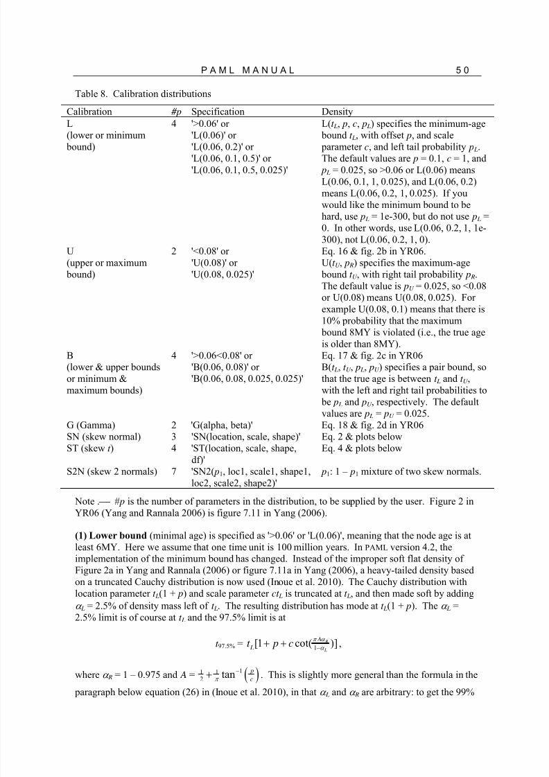
8/14/2019 pamlDOC.pdf
http://slidepdf.com/reader/full/pamldocpdf 51/70
P A M L M A N U A L 5 0
Table 8. Calibration distributions
Calibration #p Specification Density
L
(lower or minimum bound)
4 '>0.06' or
'L(0.06)' or'L(0.06, 0.2)' or'L(0.06, 0.1, 0.5)' or'L(0.06, 0.1, 0.5, 0.025)'
L(t L, p, c, p L) specifies the minimum-age
bound t L, with offset p, and scale parameter c, and left tail probability p L.The default values are p = 0.1, c = 1, and
p L = 0.025, so >0.06 or L(0.06) meansL(0.06, 0.1, 1, 0.025), and L(0.06, 0.2)means L(0.06, 0.2, 1, 0.025). If youwould like the minimum bound to behard, use p L = 1e-300, but do not use p L =0. In other words, use L(0.06, 0.2, 1, 1e-300), not L(0.06, 0.2, 1, 0).
U(upper or maximum
bound)
2 '<0.08' or'U(0.08)' or
'U(0.08, 0.025)'
Eq. 16 & fig. 2b in YR06.U(t U , p R) specifies the maximum-age
bound t U , with right tail probability p R.The default value is pU = 0.025, so <0.08or U(0.08) means U(0.08, 0.025). Forexample U(0.08, 0.1) means that there is10% probability that the maximum
bound 8MY is violated (i.e., the true ageis older than 8MY).
B(lower & upper boundsor minimum &maximum bounds)
4 '>0.06<0.08' or'B(0.06, 0.08)' or'B(0.06, 0.08, 0.025, 0.025)'
Eq. 17 & fig. 2c in YR06B(t L, t U , p L, pU ) specifies a pair bound, sothat the true age is between t L and t U ,with the left and right tail probabilities to
be p L and pU , respectively. The defaultvalues are p L = pU = 0.025.
G (Gamma) 2 'G(alpha, beta)' Eq. 18 & fig. 2d in YR06SN (skew normal) 3 'SN(location, scale, shape)' Eq. 2 & plots belowST (skew t ) 4 'ST(location, scale, shape,
df)'Eq. 4 & plots below
S2N (skew 2 normals) 7 'SN2( p1, loc1, scale1, shape1,loc2, scale2, shape2)'
p1: 1 – p1 mixture of two skew normals.
Note . # p is the number of parameters in the distribution, to be supplied by the user. Figure 2 inYR06 (Yang and Rannala 2006) is figure 7.11 in Yang (2006).
(1) Lower bound (minimal age) is specified as '>0.06' or 'L(0.06)', meaning that the node age is at
least 6MY. Here we assume that one time unit is 100 million years. In PAML version 4.2, theimplementation of the minimum bound has changed. Instead of the improper soft flat density ofFigure 2a in Yang and Rannala (2006) or figure 7.11a in Yang (2006), a heavy-tailed density basedon a truncated Cauchy distribution is now used (Inoue et al. 2010). The Cauchy distribution withlocation parameter t L(1 + p) and scale parameter ct L is truncated at t L, and then made soft by adding
L = 2.5% of density mass left of t L. The resulting distribution has mode at t L(1 + p). The L =2.5% limit is of course at t L and the 97.5% limit is at
t 97.5% =1
[1 cot( )] R
L
A
Lt p c
,
where R = 1 – 0.975 and A =
11 1
2
tan p
c
. This is slightly more general than the formula in the
paragraph below equation (26) in (Inoue et al. 2010), in that L and R are arbitrary: to get the 99%

8/14/2019 pamlDOC.pdf
http://slidepdf.com/reader/full/pamldocpdf 52/70

8/14/2019 pamlDOC.pdf
http://slidepdf.com/reader/full/pamldocpdf 53/70
P A M L M A N U A L 5 2
(5) Skew normal distribution SN(location, scale, shape) or SN(, , ) (Azzalini and Genton2007). The basic form of the skew normal distribution has density
f ( z; ) = 2 ( z)( z), (1)
where () and () are the PDF and CDF of the standard normal distribution respectively. Then x =
+ z, has the skew normal distribution SN( , , ) with location parameter , scale parameter ,
and shape parameter . The density is
f SN( x; , , ) =
2
22
2
( )
21 1 1
e2 2
xu
x
u
e d . (2)
for – < < , 0 < < , – < < . Let =21 . The mean and variance are
22 2
( ) 2 ,
Var( ) 1 .
E x
x
(3)
(6) Skew t distribution, ST(location, scale, shape, df) or ST( , , , ) (Azzalini and Genton
2007), with location parameter , scale parameter , shape parameter , and degree of freedom ,has density
2
ST
2( ; , , , ) ( ; ) ( 1) ( ); 1 f x t z T z z
, (4)
where z = ( x – )/ , t and T are the PDF and CDF of the standard t distribution, respectively. Theseare defined as follows.
2
( 1) 221
2
12
1 1 12 2 2( )
( 1)( ; ) 1 ,
, , if 0( ; )
1 ( ; ), if 0
z
zt z
I zT z
T z z
,
.
(5)
where () is the gamma function, and
1 1
0
1( , ) (1 ) d
( , )
pa b
p I a b u u u
B a b
(6)
is the incomplete beta function ratio, or the CDF of the beta(a, b) distribution, while
11 1
0
( ) ( )( , ) (1 ) d
( )
a b a b B a b u u u
a b
(7)
is the beta function.

8/14/2019 pamlDOC.pdf
http://slidepdf.com/reader/full/pamldocpdf 54/70
P A M L M A N U A L 5 3
0
0.1
0.2
0.3
0.4
0.5
0 5 10
0
0.1
0.2
0.3
0.4
0.5
0 5 10
SN(2, 1.5, 6) ST(2, 1.5, 6, 2.2)
0
0.1
0.2
0.3
0.4
0.5
-10 -5 0 5
0
0.1
0.2
0.3
0.4
0.5
-10 -5 0 5
SN(2, 1.5, –6) ST(2, 1.5, –6, 2.2)
0
0.1
0.2
0.3
0.4
0.5
0 2 4 6 8 10
0
0.1
0.2
0.3
0.4
0.5
0 2 4 6 8 10
SN(2, 1.5, 10) ST(2, 1.5, 10, 3)
0
0.1
0.2
0.3
0.4
0.5
0 5 10 15 20
0
0.1
0.2
0.3
0.4
0.5
0 5 10 15 20
SN(2, 1.5, 50) ST(2, 1.5, 50, 1)
Figure 1. Density functions for skew normal (blue) and skew t (red) distributions.
Skew t has heavier tails than skew normal.
Here are a few notes about the skew normal and skew t distributions.
When the shape parameter = 0, the distributions become the standard (symmetrical)normal and t distributions.
Changing to – flips the density at x = (the location parameter). Fossil calibrations
should have long right tails, which means > 0.
A larger | | means more skewed distributions. When | | = , the distribution is called
folded normal or folded t distribution, that is, the normal or t distribution truncated at from
the left ( = ) or from the right ( = – ).
When the degree of freedom = , the t or skew t distribution becomes the normal or skew
normal distribution. The smaller is, the heavier the tails are. A small (1-4 , say) with a
large shape parameter in the skew t distribution represents virtually hard minimal bound
and very uncertain maximal bound. When = 1, the t distribution is known as Cauchy
distribution, which does not have mean or variance.
Both skew normal and skew t distributions go from – to . In MCMCTREE, negative
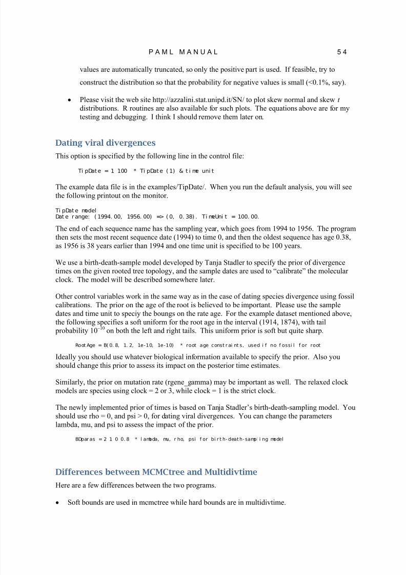
8/14/2019 pamlDOC.pdf
http://slidepdf.com/reader/full/pamldocpdf 55/70
P A M L M A N U A L 5 4
values are automatically truncated, so only the positive part is used. If feasible, try to
construct the distribution so that the probability for negative values is small (<0.1%, say).
Please visit the web site http://azzalini.stat.unipd.it/SN/ to plot skew normal and skew t distributions. R routines are also available for such plots. The equations above are for mytesting and debugging. I think I should remove them later on.
Dating viral divergences
This option is specified by the following line in the control file:
Ti pDat e = 1 100 * Ti pDat e ( 1) & t i me uni t
The example data file is in the examples/TipDate/. When you run the default analysis, you will seethe following printout on the monitor.
Ti pDat e modelDat e r ange: ( 1994. 00, 1956. 00) => ( 0, 0. 38) . Ti meUni t = 100. 00.
The end of each sequence name has the sampling year, which goes from 1994 to 1956. The programthen sets the most recent sequence date (1994) to time 0, and then the oldest sequence has age 0.38,as 1956 is 38 years earlier than 1994 and one time unit is specified to be 100 years.
We use a birth-death-sample model developed by Tanja Stadler to specify the prior of divergencetimes on the given rooted tree topology, and the sample dates are used to “calibrate” the molecularclock. The model will be described somewhere later.
Other control variables work in the same way as in the case of dating species divergence using fossil
calibrations. The prior on the age of the root is believed to be important. Please use the sampledates and time unit to speciy the boungs on the rate age. For the example dataset mentioned above,the following specifies a soft uniform for the root age in the interval (1914, 1874), with tail
probability 10 –10 on both the left and right tails. This uniform prior is soft but quite sharp.
Root Age = B( 0. 8, 1. 2, 1e-10, 1e-10) * root age const r ai nt s, used i f no f ossi l f or root
Ideally you should use whatever biological information available to specify the prior. Also youshould change this prior to assess its impact on the posterior time estimates.
Similarly, the prior on mutation rate (rgene_gamma) may be important as well. The relaxed clockmodels are species using clock = 2 or 3, while clock = 1 is the strict clock.
The newly implemented prior of times is based on Tanja Stadler’s birth-death-sampling model. Youshould use rho = 0, and psi > 0, for dating viral divergences. You can change the parameterslambda, mu, and psi to assess the impact of the prior.
BDpar as = 2 1 0 0. 8 * l ambda, mu, r ho, psi f or bi r t h- death-sampl i ng model
Differences between MCMCtree and Multidivtime
Here are a few differences between the two programs.
Soft bounds are used in mcmctree while hard bounds are in multidivtime.

8/14/2019 pamlDOC.pdf
http://slidepdf.com/reader/full/pamldocpdf 56/70

8/14/2019 pamlDOC.pdf
http://slidepdf.com/reader/full/pamldocpdf 57/70
P A M L M A N U A L 5 6
implemented in baseml or codeml, and this option should allow you to use amino acid or codonsubstitution models. The calculation of the Hessian matrix may be sensitive to the step length usedin the difference approximation, and it is advisable that you change the variable Small_Diff in thecontrol file tmp#.ctl to see whether the results are stable.
The output file out.BV from usedata = 3 should then be renamed in.BV. This file has one block ofresults for each locus. If you manually edit the control file tmp#.ctl and then invoke baseml orcodeml from the command line (for example, by typing codeml tmp2.ctl), you will have tomanually copy the content of rst1 into in.BV.
With usedata = 2, mcmctree will read the MLEs and Hessian matrix from in.BV and apply theapproximate method for calculating the likelihood in the MCMC.
In effect, mcmctree/usedata = 3 performs the function of estbranches and you can manually performthis step by running baseml or codeml externally after the tree file tmp#.ctl is generated. Similarlymcmctree/usedata = 2 performs the function of mlutidivtime.
Models of amino acid or codon substitution are not implemented in the mcmctree program for theexact likelihood calculation. The only way to use those models is through the approximate method(usedata = 3 and 2). If is advisable that you edit the intermediate control file tmp#.ctl to choose theappropriate model of amino acid or codon substitution in the codeml analysis, and then copy theresults into the in.BV file. Also have a look at the estimated branch lengths in the tree. If many ofthem are near 0, you should be concerned as perhaps you have too little data or the tree is wrong forthe locus. Finally run mcmctree/usedata = 2.
In the description here, a gene or locus means a site partition. For example, since the three codon positions typically have very different rates, different base compositions, etc., you may treat them as
separate partitions.

8/14/2019 pamlDOC.pdf
http://slidepdf.com/reader/full/pamldocpdf 58/70
P A M L M A N U A L 5 7
10 Miscelaneous notes
Also see the FAQ page, but please note that document is not up to date.
Analysing large data sets and iteration algorithms
The maximum likelihood method estimates parameters by maximizing the likelihood function. Thisis multi-dimensional optimisation problem that has to be solved numerically (see Yang 2000a for an
exception). PAML implements two iteration algorithms. The first one (met hod = 0) is a general-
purpose minimization algorithm that deals with upper and lower bounds for parameters but notgeneral equality or inequality constraints. The algorithm requires first derivatives, which arecalculated using the difference approximation, and accumulates information about the curvature(second derivatives) during the iteration using the BFGS updating scheme. At each iteration step, itcalculates a search direction, and does a one-dimensional search along that direction to determinehow far to go. At the new point, the process is repeated, until there is no improvement in the log-likelihood value, and changes to the parameters are very small. The algorithm updates all
parameters including branch lengths simultaneously.
Another algorithm (method = 1) works if an independent rate is assumed for each branch (clock = 0)(Yang 2000b). This algorithm cycles through two phases. Phase I estimates branch lengths with
substitution parameters (such as the transition/transversion rate ratio and the gamma shape
parameter ) fixed. Phase II estimates substitution parameters using the BFGS algorithm,mentioned above, with branch lengths fixed. The procedure is repeated until the algorithmconverges. In phase I of the algorithm, branch lengths are optimized one at a time. The advantageof the algorithm is that when the likelihood is calculated for different values of one single branchlength, as is required when that branch length only is optimised, much of likelihood calculations on
the phylogeny is the same and can be avoided by storing intermediate results in the computermemory. A cycle is completed after all branch lengths are optimized. As estimates of branchlengths are correlated, several cycles are needed to achieve convergence of all branch lengths in thetree, that is, to complete phase I of the algorithm.
If branch lengths are the only parameters to be estimated, that is, if substitution parameters are fixed,the second algorithm (method = 1) is much more efficient. Thus to perform heuristic tree search
using stepwise addition, for example, you are advised to fix substitution parameters (such as and
). The second algorithm is also more efficient if the data contain many sequences so that the treehas many branch lengths.
Tip: To get good initial values for large data sets of protein coding DNA sequences, you can use
baseml. Add the options characters “GC” at the end of the first line in the sequence data file. Thenrun the data with baseml. In the result file generated by baseml (say mlb), look for “branch lengthsfor codon models” and copy the tree with branch lengths into the tree file. Then run codeml andchoose “1: initial values” when asked about what to do with the branch lengths in the tree.
Tree search algorithms
One heuristic tree search algorithm implemented in baseml , codonml and aaml is a divisive
algorithm, called "star-decomposition" by Adachi and Hasegawa (1996b). The algorithm starts from
either the star tree (r unmode = 2) or a multifurcating tree read from the tree structure file
(r unmode = 1). The algorithm joins two taxa to achieve the greatest increase in log-likelihood over
the star-like tree. This will reduce the number of OTUs by one. The process is repeated to reduce thenumber of OTUs by one at each stage, until no multifurcation exists in the tree. This algorithmworks either with or without the clock assumption. The stepwise addition algorithm is implemented

8/14/2019 pamlDOC.pdf
http://slidepdf.com/reader/full/pamldocpdf 59/70
P A M L M A N U A L 5 8
with the option r unmode = 3. Options r unmode = 4 or 5 are used for nearest neighbor
interchanges , with the intial tree determined with stepwise addition under the parsimony criterion
(r unmode = 4) or read from the tree structure file (r unmode = 5). The results are self-explanatory.
Besides the fact that ML calculations are slow, my implementations of these algorithms are crude.
If the data set is small (say, with <20 or 30 species), the stepwise addition algorithm (r unmode = 3)
appears usable. Choose cl ock = 0, and met hod = 1 to use the algorithm that updates one branch
at a time, and fix substitution parameters in the model (such as and ) so that only branch lengths
are optimized. Parameters and can be fixed in the tree search using f i x_kappa and
f i x_al pha in the control files. Other parameters (such as substitution rates for genes or codon
positions or site partitions) cannot be fixed this way; they can instead be specified in the file of
initial values (i n. baseml or i n. codeml ). Suppose you use a candidate tree to estimate branch
lengths and substitution parameters with r unmode = 0. You can then move the substitution
parameters (but not the branch lengths) into the file of initial values. You then change the following
variables for tree search: r unmode = 3, met hod = 1. The program will use the substitution
parameters as fixed in the tree search, and optimizes branch lengths only. It is important that thesubstitution parameters are in the right order in the file; so copy-and-paste from PAML output is
probably the safest. It is also important that you do not change the parameter specifications in thecontrol file; the control file should indicate that you want to estimate the substitution parameters, butwhen the program detects the file of initial values, fixed parameter values are used instead.
Generating bootstrap data sets
To generate bootstrap pseudo-samples from your original data, you should use the control variable
boot st r ap in the control files baseml . ct l or codeml . ct l , and specify the number of
samples, as follows.
boot st r ap = 100 * generat e bootst r ap data sets
This generates a file named boot.txt. The file name is hard coded in the programs so you mightwant to rename it. Note that the way bootstrap samples are generated depends on your model, soyou use baseml to generate samples for nucleotide-based analysis and codeml for amino acid andcodon-based analysis. If the data are partitioned (using option G), the programs use stratifiedsampling to generate bootstrap samples, preserving the number of sites in each partition.
The bootstrap samples can be analyzed using phylip programs (choose the option for multiple data
sets) and baseml or codeml (using the variable ndat a in the control file).
The rub file recording the progress of iteration
If you use a large value for the variable noisy (say >2), the programs baseml and codeml will log
output to the screen, indicating the progress of the iteration process, i.e., the minimization of the
negative log-likelihood. They will also print in the r ub file, the size (norm) of the gradient or searchdirection (h), the negative log likelihood, and the current values of parameters for each round ofiteration. A healthy iteration is indicated by the decrease of both h and the negative log likelihood,and h is particularly sensitive. If you run a complicated model hard to converge or analyzing a largedata set with hundreds or thousands of sequences, you may switch on the output. You can check thisfile to see whether the algorithm has converged. A typical symptom of failure of the algorithm isthat estimates of parameters are at the preset boundaries, with values like 2.00000, 5.00000. When
met hod = 1, the output in the r ub file lists the log likelihood and parameter estimates only.

8/14/2019 pamlDOC.pdf
http://slidepdf.com/reader/full/pamldocpdf 60/70
P A M L M A N U A L 5 9
Specifying initial values
You may change values of parameters in the control file such as kappa, alpha, omega, etc. to startthe iteration from different initial values. Initial values for the second and later trees are determined
by the program, and so you do not have much control in this way.
You can collect initial values into a file called i n. baseml if you are running baseml or
i n. codeml if you are running codeml . This file should contain as many numbers, separated by
white spaces, as the number of parameters that are being optimized by the program. So if the program is estimating 56 parameters (say 51 branch lengths, 1 kappa, and 5 other parameters from
the distribution), you should put 56 numbers in the file. The parameters are ordered internally inthe program and you have no control of the ordering. Nevertheless, the order is the same as in themain output (below the lnL line for each tree). One way of generating the in.codeml or in.basemlfiles is to run a data set, and then copy initial values from the rub file or from the main output file.
The r ub file records the iteration process and has one line for each round of iteration. Each line lists
the current parameter values after the symbol x; you can copy those numbers (not the symbol x) intothe file of initial values, and if you like, change one or a few of the parameter values too. When yourun the program, look at lnL0 printed out on the screen and check that it is the same as recorded inrub.
When the program runs, it checks to see whether a file of initial values exists, and it does, the program will read initial values from it. This may be useful if the iteration is somehow aborted, and
then you can collect current values of parameters from the file r ub into this file of initial values, sothat the new iteration can have a better start and may converge faster. The file of initial values mayalso be useful if you experience problems with convergence. If you have already obtained
parameter estimates before and do not want the program to re-estimate them and only want to dosome analysis based on those estimates such as reconstructing ancestral sequences, insert -1 before
the initial values.
Warning: A complication is that in some models a transformation is applied during the iterationwhile the printout uses the original variables. Examples of this are the frequency/proportion
parameters for base frequencies (nhomo = 1 in baseml), proportions of site classes in the NSsitesmodels (except for models always having only two classes in which case no transformation isapplied), and times or node ages in clock models (clock = 1, 2, 3, 5, 6, but not 0). For those models,you can see that the line of output in the main output file looks different from the last line of rubafter the iteration finishes. In the file of initial values, if you use -1 at the start, the program assumesthe original variables, while if you don’t, the program assumes transformed variables.
Fine-tuning the iteration algorithm
The iteration algorithm uses the difference approximation to calculate derivatives. This methodchanges the variable ( x) slightly, say by a small number e, and see how the function value changes.
One such formula is d f /d x = [ f ( x + e) f ( x)]/e. The small number e should be small to allow accurateapproximation but should not be too small to avoid rounding errors. You can change this value by
adding a line in the control files baseml . ct l or codeml . ct l
Smal l _Di f f = 1e- 6
The iteration is rather sensitive to the value of this variable, and reasonable values are between 1e-5and 1e-7. This variable also affects the calculation of the SE's for parameters, which are much moredifficult to approximate than the first derivatives. If the calculated SE's are sensitive to slight changein this variable, they are not reliable.

8/14/2019 pamlDOC.pdf
http://slidepdf.com/reader/full/pamldocpdf 61/70

8/14/2019 pamlDOC.pdf
http://slidepdf.com/reader/full/pamldocpdf 62/70
P A M L M A N U A L 6 1
or type in the file name when prompted by neighbour. Then type L to tell the program that thematrix if lower-diagonal.
PAUP, MacClade, and MrBayes
Sequence data file. PAUP, MacClade and MrBayes use the so-called NEXUS file format. PAML programs (mainly baseml and codeml) have some limited support for this format and can read thesequence alignment in that format. Only the sequence alignment is read and the command blocksare ignored. Also PAML does not recognise comments inside the sequence data block, so pleaseavoid them.
The program evolver in the paml package can generate data sets both in the PAML/PHYLIP formatand in the PAUP/MrBayes nexus format. You can also modify the file paupblock to add blocks of
paup or MrBayes command at the end of each simulated data set. See the descriptions for theevolver program in Chapter
Tree file . PAML programs have only limited support with the tree file generated by PAUP orMacClade. First the “[&U]” notation for specifying an unrooted tree is not recognised. For a tree to
be accepted as an unrooted tree by PAML, you have to manually modify the tree file and delete a pair of parenthesis so that there is a trifurcation at the root; that is, the outmost pair of parenthesesgroups together three taxa rather than two, so the tree should be in the format (A, B, C). Thuschanging “(((1,2),3),4)” into “((1,2),3,4)” will deroot the tree. Perhaps I should let the program to dothis automatically. Second, the “Translate” keyword is ignored by PAML, and it is assumed that theordering of the sequences in the tree file is exactly the same as the ordering of the sequences in thesequence data file. This seems normally the case if the trees are reconstructed from the samesequence file using paup.
Clustal
Sequence data file. When you save the clustal alignment in the PHYLIP format with extension.phy, clustal output the alignment using the “interleaved” phylip format, truncating sequence namesto 10 characters. This file is typically not readable by PAML programs. You need to make twochanges. First add the letter I at the end of the first line, after the number of sequences and thenumber of sites in the sequence. Second, add spaces between the sequence name and the sequenceand make sure there are at least two spaces separating the name and the sequence.
MEGA
Sequence data file. The MEGA sequence data format (Kumar et al. 1994) is different and notdirectly readable by PAML programs. Need to find out about the format and write something here.
MOLPHY
Sequence data file. It is possible to prepare the same file to be readable by both MOLPHY programs (nucml and protml) and PAML programs. Need to find out about the format and writesomething here.
The tree file produced by MOLPHY also uses the parenthesis notation and is readable by PAML programs.
FigTree
Andrew Rambaut’s FigTree can be used to view trees produced using paml programs.

8/14/2019 pamlDOC.pdf
http://slidepdf.com/reader/full/pamldocpdf 63/70
P A M L M A N U A L 6 2
TreeView
The trees with branch lengths calculated from PAML programs should be directly readable byTreeView (Page 1996). You can copy the tree onto the clipboard and paste into TreeView, or save
the tree in a file and read the file from within TreeView. Some of the models implemented in baseml and codeml require the user to label branches or nodes on the tree, and I found TreeView particularly useful for this purpose when the tree is large. TreeView shows those labels as node
labels. For example, the free-ratios model in codonml (model = 1) estimates one ratio for each
branch. In the output, codeml prints out a tree with the estimated ratio as node/branch labels, withsome notes like “Tree for Rod Page’s TreeView”. I can copy this tree into tree view. Similarly theglobal and local clock models in baseml and codeml estimate an age for each node, and the outputtree from those two programs can be copied into TreeView directly.
Andrew Rambaut’s TreeEdit, which runs on MACs, has similar functionalities. However, I don’thave MAC and have no experience with the program.
Windows notes
Turn on file extensions in Windows Explorer. Windows Explorer by default hides file extensionsfor known file types. You should go to "Windows Explorer - Tools - Folder options - View" andun-tick "Hide extensions for known file types", so that you can see the full file names fromWindows Explorer.
Using Task Manger to change job priority. Start Task Manger (for example, right click on task barand choose Task Manager). Click on Processes button. Locate the big job, say, codeml. Right clickand Set Priority to Low. Note that the process running the Command Prompt is cmd. If you changethe priority of cmd to low, all jobs started from that window will run at low priority. You canchange View – Update Speed to Low and change View – Select Columns. Change Options –
Minimize on Use. Then you can minimize rather than close Task Manger.
All input and output files are plain text files. In the Command Prompt box (Start - Programs –Accessaries – Command Prompt), you can use type or more to view a text file. If you see strangecharacters on the screen and perhaps also hear beeps, the file is not a plain text file. You can alsouse a text editor to view and edit a plain text file. If you use Microsoft Word or Wordpad to save afile, make sure that the files are saved as a plain text file. Use File – Save As and change the filetype. When you do, Word or other programs might automatically add the file extension .txt, andyou will have to rename the file if you don’t want the .txt.
How to change your search path to include paml programs. You can create a folder called binunder your account. The folder name should be shown when you move (cd ) to that folder. Let’s
say this is D:\bin. Copy or move the executable files from the paml/bin/ folder into this folder.
Now change the environment variable path. On Windows Vista or XP, open Control Panel –System – Advanced System Settings – Environment variables. Under “User variables for Ziheng”,find path, and Edit. Add the folder name (D:\bin in my example) to the end or beginning of thestring. The fields are separated by semi-colons. Note that Windows/Dos is case-insensitive, soD:\bin is the same as D:\BIN or d:\bin.
UNIX/Linux/Mac OSX notes
How to change your search path to include paml programs. You can create a folder bin in yourroot directory and copy paml executables into that folder, and then include the folder in your search
path. This way you can run the program no matter where you are. If you have several versions of

8/14/2019 pamlDOC.pdf
http://slidepdf.com/reader/full/pamldocpdf 64/70
P A M L M A N U A L 6 3
the paml, you may even name the executables baseml3.15, baseml4, etc., to distinguish them.Similarly you can copy other programs such as mb, dnadist, etc. into that folder.
Type cd to move to your root directory. Create a bin/ folder in your root directory.
mkdir bin
Copy executables such as codeml, baseml, and mcmctree into the bin/ folder.
Then modify your path environment variable to include the bin/ folder in the initialization filefor the shell. You can use more /etc/passwd to see which shell you run. Below are notes for the Cshell and bash shell. There are other shells, but these two are commonly used.
1) If you see /bin/csh for your account in the /etc/passwd file, you are running the C shell, andthe intialization file is .cshrc in your root folder. You can use more .cshrc to see itscontent if it is present. Use a text editor (such as emacs, vi, SimpleText, etc.) to edit the file,and insert the following line
set path = ($path . ~/bin)
The different fields are separated by spaces. Here . means the current folder, and ~/ meansyour root folder, and ~/bin means the bin folder you created, and $path is whatever foldersare already in the path.If the file .cshrc does not exist, you create one, and insert the line above.
2) If you see /bin/bash in the file /etc/passwd for your account, you are running the bash shell,and the initialization file is .bashrc. Use a text editor to open .bashrc and insert thefollowing line
PATH=$PATH:./:~/bin/
This changes the environment variable PATH. The different fields are separated by colon :and not space. If the file does not exist, create one.
After you have changed and saved the initialization file, every time you start a shell, the path isautomatically set for you.
Note that UNIX is case-sensitive.

8/14/2019 pamlDOC.pdf
http://slidepdf.com/reader/full/pamldocpdf 65/70
P A M L M A N U A L 6 4
11 References
Adachi, J., and M. Hasegawa. 1996a. Model of amino acid substitution in proteins encoded by
mitochondrial DNA. Journal of Molecular Evolution 42:459-468.
Adachi, J., and M. Hasegawa. 1996b. MOLPHY Version 2.3: Programs for molecular phylogenetics based on maximum likelihood. Computer Science Monographs, 28:1-150. Institute ofStatistical Mathematics, Tokyo.
Anisimova, M., J. P. Bielawski, and Z. Yang. 2001. The accuracy and power of likelihood ratio teststo detect positive selection at amino acid sites. Molecular Biology and Evolution 18:1585-1592.
Anisimova, M., J. P. Bielawski, and Z. Yang. 2002. Accuracy and power of Bayes prediction ofamino acid sites under positive selection. Molecular Biology and Evolution 19:950-958.
Anisimova, M., R. Nielsen, and Z. Yang. 2003. Effect of recombination on the accuracy of thelikelihood method for detecting positive selection at amino acid sites. Genetics 164:1229-1236.
Azzalini, A., and M. G. Genton. 2007. Robust likelihood methods based on the skew-t and relateddistributions. Int. Statist. Rev. 76:106-129.
Bielawski, J. P., and Z. Yang. 2004. A maximum likelihood method for detecting functionaldivergence at individual codon sites, with application to gene family evolution. Journal ofMolecular Evolution 59:121-132.
Bishop, M. J., and A. E. Friday. 1987. Tetropad relationships: the molecular evidence. Pp. 123-139in C. Patterson, ed. Molecules and Morphology in Evolution: Conflict or Compromise?Cambridge University Press, Cambridge, England.
Brown, W. M., E. M. Prager, A. Wang, and A. C. Wilson. 1982. Mitochondrial DNA sequences of primates: tempo and mode of evolution. Journal of Molecular Evolution 18:225-239.
Chang, B. S., and M. J. Donoghue. 2000. Recreating ancestral proteins. Trends Ecol. Evol. 15:109-114.
Dayhoff, M. O., R. M. Schwartz, and B. C. Orcutt. 1978. A model of evolutionary change in proteins. Pp. 345-352. Atlas of protein sequence and structure, Vol 5, Suppl. 3. NationalBiomedical Research Foundation, Washington D. C.
DeBry, R. W. 1992. The consistency of several phylogeny-inference methods under varyingevolutionary rates. Molecular Biology and Evolution 9:537-551.
Felsenstein, J. 1981. Evolutionary trees from DNA sequences: a maximum likelihood approach.Journal of Molecular Evolution 17:368-376.
Felsenstein, J. 2004. Inferring Phylogenies. Sinauer Associates, Sunderland, Massachusetts.
Felsenstein, J. 2005. Phylip: Phylogenetic Inference Program, Version 3.6. University ofWashington, Seattle.
Fitch, W. M. 1971. Toward defining the course of evolution: minimum change for a specific treetopology. Systematic Zoology 20:406-416.
Forsberg, R., and F. B. Christiansen. 2003. A codon-based model of host-specific selection in parasites, with an application to the influenza A virus. Molecular Biology and Evolution20:1252-1259.
Galtier, N., and M. Gouy. 1998. Inferring pattern and process: maximum-likelihood implementationof a nonhomogeneous model of DNA sequence evolution for phylogenetic analysis. Molecular
Biology and Evolution 15:871-879.

8/14/2019 pamlDOC.pdf
http://slidepdf.com/reader/full/pamldocpdf 66/70
8/14/2019 pamlDOC.pdf
http://slidepdf.com/reader/full/pamldocpdf 67/70
P A M L M A N U A L 6 6
Pauling, L., and E. Zuckerkandl. 1963. Chemical paleogenetics: molecular "restoration studies" ofextinct forms of life. Acta Chem. Scand. 17:S9-S16.
Pupko, T., I. Pe'er, R. Shamir, and D. Graur. 2000. A fast algorithm for joint reconstruction of
ancestral amino acid sequences. Molecular Biology and Evolution 17:890-896.Rannala, B., and Z. Yang. 1996. Probability distribution of molecular evolutionary trees: a new
method of phylogenetic inference. Journal of Molecular Evolution 43:304-311.
Rannala, B., and Z. Yang. 2007. Inferring speciation times under an episodic molecular clock.Systematic Biology 56:453-466.
Robinson, D. F., and L. R. Foulds. 1981. Comparison of phylogenetic trees. Math. Biosci. 53:131-147.
Saitou, N., and M. Nei. 1987. The neighbor-joining method: a new method for reconstructing phylogenetic trees. Molecular Biology and Evolution 4:406-425.
Self, S. G., and K.-Y. Liang. 1987. Asymptotic properties of maximum likelihood estimators andlikelihood ratio tests under nonstandard conditions. J. Am. Stat. Assoc. 82:605-610.
Shimodaira, H., and M. Hasegawa. 1999. Multiple comparisons of log-likelihoods with applicationsto phylogenetic inference. Molecular Biology and Evolution 16:1114-1116.
Stewart, C.-B., J. W. Schilling, and A. C. Wilson. 1987. Adaptive evolution in the stomachlysozymes of foregut fermenters. Nature 330:401-404.
Suzuki, Y., and T. Gojobori. 1999. A method for detecting positive selection at single amino acidsites. Molecular Biology and Evolution 16:1315-1328.
Swanson, W. J., R. Nielsen, and Q. Yang. 2003. Pervasive adaptive evolution in mammalianfertilization proteins. Molecular Biology and Evolution 20:18-20.
Tamura, K. 1992. Estimation of the number of nucleotide substitutions when there are strongtransition-transversion and G+C content biases. Molecular Biology and Evolution 9:678-687.
Tamura, K., and M. Nei. 1993. Estimation of the number of nucleotide substitutions in the controlregion of mitochondrial DNA in humans and chimpanzees. Molecular Biology and Evolution10:512-526.
Thorne, J. L., H. Kishino, and I. S. Painter. 1998. Estimating the rate of evolution of the rate ofmolecular evolution. Molecular Biology and Evolution 15:1647-1657.
Thornton, J. 2004. Resurrecting ancient genes: experimental analysis of extinct molecules. Nat. Rev.Genet. 5:366-375.
Whelan, S., and N. Goldman. 2001. A general empirical model of protein evolution derived from
multiple protein families using a maximum likelihood approach. Molecular Biology andEvolution 18:691-699.
Whelan, S., P. Liò, and N. Goldman. 2001. Molecular phylogenetics: state of the art methods forlooking into the past. Trends Genet. 17:262-272.
Wong, W. S. W., Z. Yang, N. Goldman, and R. Nielsen. 2004. Accuracy and power of statisticalmethods for detecting adaptive evolution in protein coding sequences and for identifying
positively selected sites. Genetics 168:1041-1051.
Yang, Z. 1993. Maximum-likelihood estimation of phylogeny from DNA sequences whensubstitution rates differ over sites. Molecular Biology and Evolution 10:1396-1401.
Yang, Z. 1994a. Maximum likelihood phylogenetic estimation from DNA sequences with variablerates over sites: approximate methods. Journal of Molecular Evolution 39:306-314.

8/14/2019 pamlDOC.pdf
http://slidepdf.com/reader/full/pamldocpdf 68/70

8/14/2019 pamlDOC.pdf
http://slidepdf.com/reader/full/pamldocpdf 69/70

8/14/2019 pamlDOC.pdf
http://slidepdf.com/reader/full/pamldocpdf 70/70
P A M L M A N U A L 6 9
Index
aaDist ..........................................................................35alignment.......................................................................5alignment gap ....................... ....................... ................12alpha ...........................................................................22ambiguity characters....................................................12ancestral reconstruction
joint ...................... ....................... ....................... .....25marginal ...................... ........................ ....................25
ancestral reconstruction ...................... .........4, 10, 24, 25BEB ....................... ....................... ....................... ........31BFGS...........................................................................57BioEdit ....................... ....................... ....................... .....5 birth-death process................ ......................... ........40, 46
bootstrap .................... ...................... ....................... .....58branch label...........................................................16, 29clade label ...................................................................16cleandata................................................................12, 26clock ....................... ....................... .. 9, 15, 21, 26, 28, 34CLUSTAL...............................................................5, 61codon model
branch model..................... ........................ ....9, 29, 35 branch-site model ..............................................31, 36clade model .............................................................32site model ....................... ....................... ........9, 30, 35
codon position ...............................12, 13, 21, 25, 29, 34CodonFreq .................................................................34convergence...........................................................57, 59
evol ver ....................................................................39
examples......................................................................10fix_alpha .....................................................................22fix_blength..................................................................26fix_kappa ....................................................................22fix_rho ........................................................................23fossil ..................... ....................... .................... 17, 21, 34GenDoc..........................................................................5gene prediction .................... ....................... ...................6genetic code.................................................................25getSE ...........................................................................24icode ................................................................26, 36, 37in.baseml......................................................................59in.codeml ....................... ...................... ....................... .59initial values ..................... ....................... ........26, 58, 59
likelihood ratio test ....................... ........................ ...5, 24LRT ........................................... See likelihood ratio test
lysozyme .......................................................................9MacClade ..................... ...................... ....................... ..61
MCaa. dat ..................................................................39
MCbase. dat .............................................................39
MCcodon. dat ..........................................................39
MEGA.........................................................................61method..................................................................26, 57Mgene..................... ......................... .... 11, 19, 20, 21, 25missing data.................................................................12model ..............................................................20, 35, 37MOLPHY....................................................................61Monte Carlo simulation...............................................41mouse lemurs ................................................................9
MrBayes......................................................................61ncatG ..........................................................................22
ndata.........................................................................21
NEB........................ ...................... ....................... ........ 31nhomo.........................................................................23noisy............................................................................20nonhomogeneous models ....................... ..................... 23nparK .........................................................................23 NSsites ...................... ...................... ....................... .9, 35OmegaAA.dat ............................................................35optimization.................................................................57Option G...........11, 12, 13, 20, 21, 22, 25, 27, 37, 58, 60outfile..........................................................................20PAUP ..........................................................................61
PHYLIP.......................................................................60RateAncestor ...................... ...................... . 24, 31, 37, 38rho...............................................................................23runmode ...............................................................20, 35seqfile..........................................................................20Small_Diff ............................................................25, 59tree
parenthesis notation ....................... ........................ .15rooted......................................................................15unrooted .................... ....................... ...................... .15
tree search....................... ........................ ........... 6, 20, 57TreeAlign ..................... ....................... ....................... ...5treefile.........................................................................20TreeView...............................................................16, 62verbose........................................................................20