TESIS - Instituto Politécnico Nacional · 2016-10-11 · junto a la pileta para lavar la ropa....
220
ANÁLISIS TEMPORAL DEL ROL DE LOS PECES EN LOS PROCESOS DE AUTO-ORGANIZACIÓN DE LA LAGUNA DE TÉRMINOS, MÉXICO TESIS QUE PARA OBTENER EL GRADO DE DOCTOR EN CIENCIAS MARINAS PRESENTA FABIÁN DAVID ESCOBAR TOLEDO LA PAZ, B.C.S., JUNIO DE 2016 INSTITUTO POLITECNICO NACIONAL CENTRO INTERDISCIPLINARIO DE CIENCIAS MARINAS ´
Transcript of TESIS - Instituto Politécnico Nacional · 2016-10-11 · junto a la pileta para lavar la ropa....

ANÁLISIS TEMPORAL DEL ROL DE LOS PECES EN LOS PROCESOS DE AUTO-ORGANIZACIÓN
DE LA LAGUNA DE TÉRMINOS, MÉXICO
TESIS
QUE PARA OBTENER EL GRADO DE
DOCTOR EN CIENCIAS MARINAS
PRESENTA
FABIÁN DAVID ESCOBAR TOLEDO
LA PAZ, B.C.S., JUNIO DE 2016
INSTITUTO POLITECNICO NACIONAL CENTRO INTERDISCIPLINARIO DE CIENCIAS MARINAS
´

INSTITUTO POLITÉCNICO NACIONAL SECRETARÍA DE INVESTIGACIÓN Y POSGRADO
CARTA CESIÓN DE DERECHOS
En la Ciudad de La Paz, B.C.S., el día 15 del mes de Junio del año 2016
El (la) que suscribe MC. FABIÁN DAVID ESCOBAR TOLEDO Alumno (a) del Programa
DOCTORADO EN CIENCIAS MARINAS
con número de registro B120649 adscrito al CENTRO INTERDISCIPLINARIO DE CIENCIAS MARINAS
manifiesta que es autor(a) intelectual del presente trabajo de tesis, bajo la dirección de:
DR. MANUEL JESÚS ZETINA REJÓN
y cede los derechos del trabajo titulado:
“ANÁLISIS TEMPORAL DEL ROL DE LOS PECES EN LOS PROCESOS
DE AUTO-ORGANIZACIÓN DE LA LAGUNA DE TÉRMINOS, MÉXICO”
al Instituto Politécnico Nacional, para su difusión con fines académicos y de investigación.
Los usuarios de la información no deben reproducir el contenido textual, gráficas o datos del trabajo
sin el permiso expreso del autor y/o director del trabajo. Éste, puede ser obtenido escribiendo a la
siguiente dirección: [email protected] - [email protected]
Si el permiso se otorga, el usuario deberá dar el agradecimiento correspondiente y citar la fuente del
mismo.
MC. FABIÁN DAVID ESCOBAR TOLEDO
Nombre y firma del alumno

La disciplina tarde o temprano vencerá a la inteligencia
(Proverbio Japonés)
“… La comadre Carmen, que no es comadre mía sino que a así la llaman, nos recibe
sentada en taburete inclinado contra una columna de madera, de espaldas a un
espacioso patio bañado de ráfagas de sol que se cuelan entre las ramas de dos
frondosos y alargados árboles de mamón. Tres niños flacos y barrigones del color del
chocolate, de entre cinco y ocho años, algarabían el ambiente jugando desnudos
junto a la pileta para lavar la ropa. Siete gallinas, un gallo y dos perros de raza
incierta corren por igual de un lado a otro, mientras un par de gatos blanquicenizos
sestean estirados con desdén, uno sobre una mesa de madera que sirve como
comedor y otro sobre sillón viejo de cuyos cojines rotos sobresale un pedazo de
algodón ennegrecido…”
Líbranos del bien (Alfonso Sánchez Baute)

AGRADECIMIENTOS Agradecer al CONACyT y al programa Institucional de Formación de Investigadores del Instituto Politécnico Nacional (PIFI-IPN) por el apoyo económico otorgado. A los proyectos de Investigación ANR-CONACyT (11465), SIP (20161883); SEP-CONACYT: (155900, 221705) y AMEXCID-AUCI. Al Dr. Manuel Zetina-Rejón, por su dirección, amistad, certeros consejos y sobretodo el apoyo en los momentos más difíciles durante estos últimos cuatro años. Gracias por siempre estar ahí. Al comité tutorial y evaluador: Dr. Francisco Arreguín Sánchez, Dr. José De la Cruz-Agüero, Dra. Julia Ramos Miranda, Dr. Deivis S. Palacios Salgado y Dr. Rodrigo Moncayo Estrada. A los amigos que han estado cerca y los que no, los del día a día y los que por la distancia no ha sido fácil volver a vernos pero mantenemos el contacto. Ustedes son parte importante de esto. Sea esta la oportunidad para reconocerle a cinco de ellos lo valiosos que son para mí, porque disfrutaron de mis triunfos, me acompañaron en la derrota y sobre todo me dieron todo su apoyo cuando la salud menguó: Carlos Julio, Angie, Juan Carlos, Norberto y Michelle, les estaré agradecido toda la vida. A mi familia, mi mayor motivación y mi soporte. Cuando gané y cuando perdí, cuando acerté y me equivoqué, siempre estuvieron para mí. Por su esfuerzo, por su cuidado, por su cariño y por su sacrifico, gracias a todos, gracias familia. Y por supuesto, a mí querida Margarita Rosa, por todos sus sacrificios, amor y comprensión. Sé que estos cuatro años han sido una montaña rusa, pero estoy seguro que muy pronto empezaremos a recoger los frutos de tantos sacrificios.

I
ÍNDICE
ÍNDICE DE FIGURAS ................................................................................................. iii
ÍNDICE DE TABLAS ................................................................................................... vi
GLOSARIO ................................................................................................................. vii
RESUMEN ................................................................................................................... x
ABSTRACT ................................................................................................................. xi
1. ANTECEDENTES Y DESCRIPCIÓN GENERAL ....................................................1
1.1. INTRODUCCIÓN GENERAL ..............................................................................2
1.2. OBJETIVOS .......................................................................................................4
1.2.1. General .....................................................................................................4
1.2.2. Específicos ...............................................................................................4
1.3. HIPÓTESIS ........................................................................................................5
1.4. METODOLOGÍA GENERAL ...............................................................................5
1.4.1. Área de estudio .........................................................................................5
1.4.2. Procedencia de los datos .........................................................................8
1.4.3. Análisis de los datos .................................................................................9
1.4.3.1. Análisis de diversidad funcional ................................................... 10
1.4.3.2. Análisis del rol funcional ............................................................... 10
2. ANÁLISIS TEMPORAL DE LA DIVERSIDAD FUNCIONAL ................................. 11
2.1. Cambios temporales en las características funcionales de la comunidad de
peces en la Laguna de Términos en tres periodos (1980, 1998 y 2011) .................... 12
2.1.1. Introducción ............................................................................................ 12
2.1.2. Análisis de los datos ............................................................................... 15
2.1.2.1. Índice de diversidad de atributos funcionales .............................. 15
2.1.2.2. Análisis Multivariado .................................................................... 18

II
2.1.3. Resultados .............................................................................................. 19
2.1.4. Discusión ................................................................................................ 23
3. EQUIVALENCIA FUNCIONAL DE LA COMUNIDAD DE PECES ........................ 29
3.1. Equivalencia funcional de la comunidad de peces en Laguna de Términos en
tres periodos (1980, 1998 y 2011). ............................................................................. 30
3.1.1. Introducción ............................................................................................ 30
3.1.2. Análisis de los datos ............................................................................... 31
3.1.3. Resultados .............................................................................................. 33
3.1.4. Discusión ................................................................................................ 37
4. ANÁLISIS FUNCIONAL DE LOS PECES A NIVEL DEL ECOSISTEMA ............. 42
4.1. El rol de la ictiofauna en los procesos de auto-organización en la Laguna de
Términos .................................................................................................................... 43
4.1.1. Introducción ............................................................................................ 43
4.1.2. Análisis de los datos ............................................................................... 44
4.1.3. Resultados .............................................................................................. 47
4.1.4. Discusión ................................................................................................ 53
5. DISCUSIÓN GENERAL ........................................................................................ 58
6. CONCLUSIONES GENERALES .......................................................................... 64
REFERENCIAS .......................................................................................................... 67
ANEXOS

iii
ÍNDICE DE FIGURAS
Figura 1.1. Área de estudio. Los cuadros indican los puntos de muestreo para el
periodo 1980/81 y los círculos para los periodos 1998/99 y 2010/11. ..........................6
Figura 2.1. Valores del FADI para: (a) promedio anual, (b) media por época y (d)
promedio mensual. Colores en los símbolos representan los tres períodos evaluados:
negro=1980, gris=1998 y blanco=2011. Se muestra la distribución de probabilidad del
95% y el valor medio para el número de especies. Esta distribución se realizó con un
remuestreo bootstrap (1000 muestras). ..................................................................... 20
Figura 2.2. Ordenación (MDS) de los rasgos funcionales (negrita) y las variables
ambientales (cursiva). TL=Nivel Trófico, RG=Gremio Reproductivo, TG=Gremio
Trófico, BS=Forma del Cuerpo, MT=Tipo de Boca, CF=Aleta Caudal, ML=Longitud
Máxima, HA=Hábitat, UE=Uso de Estuarios, EH=Hábitat Esencial, ST=Tolerancia a
la Salinidad, DEP=Profundidad, TRA=Transparencia, SST=Temperatura Superficial,
BST=Temperatura del Fondo, SSS=Salinidad superficial y BSS=Salinidad del Fondo.
................................................................................................................................... 21
Figura 2.3. Ordenación de Componentes Principales de los rasgos funcionales
(línea continua) de cada mes en los tres períodos analizados. Colores del símbolo
representan los tres períodos evaluados: negro: 1980, gris: 1998 y blanca: 2011. TL
= Nivel Trófico, RG = Gremio Reproductivo, TG = Gremio Trófico, BS = Forma del
Cuerpo, MT = Tipo de Boca, CF = Aleta Caudal, ML = Longitud Máxima, HA =
Hábitat, UE = Uso de Estuarios, EH = Hábitat Esencial, y ST = Tolerancia a la
Salinidad. Además, las variables ambientales (línea punteada) se proyectan para
fines de interpretación. DEP = Profundidad, TRA = Transparencia, SST =
Temperatura Superficial, y SSS = salinidad superficial. ............................................. 22
Figura 3.1. Arreglo jerárquico a partir del análisis de equivalencia regular
utilizando una matriz de atributos funcionales. ........................................................... 35

iv
Figura 3.2. Análisis de diversidad funcional usando el FADI entre los bloques
formados en al análisis de equivalencia de cada periodo analizado. La línea punteada
indica el valor del FADI calculado para el periodo indicado. ...................................... 36
Figura 3.3. Análisis de clasificación jerárquica mediante el índice de similitud de
Jaccard. Se indican los años y los bloques resultantes del análisis de equivalencia
resultante en cada periodo utilizando el método de vinculación promedio. ................ 37
Figura 4.1. Matriz de correlaciones entre algunos de los indicadores ecológicos
(datos de entrada al modelo, valores estimados del análisis ecosistémico e índice de
diversidad funcional). ................................................................................................. 48
Figura 4.2. Diagrama de dispersión para visualizar la tendencia entre los índices
seleccionados para los grupos de peces en1980 (arriba), 1998 (medio) y 2011
(abajo): Ro contra (A/C)i y D. Los símbolos en negro indican especies de peces de
nivel trófico superior a tres y los rojos niveles tróficos inferiores a tres. AGU: Agujas,
ANC: Anchovetas, ANG: Anguilas, BAG: Bagres, BAR: Barbudos, CIN: Cintillas,
COR: Corvinas, IGU: Iguanas, ISA: Isabelitas, JUR: Jureles, LIS: Lisas, MER: Meros,
MOJ: Mojarras, MOM: Mojarras mexicanas, PAR: Pargos, GLO: Peces Globo, PLA:
Peces Planos, ROC: Peces Roca, PEJ: Pejesapos, PER: Pericos, RAY: Rayas, ROB:
Robalos, RON: Roncos, SAR: Sardinas, SAG: Sargos. ............................................. 50
Figura 4.3. Diagrama de dispersión para la visualización de la tendencia entre
los índices Ro y TL para los periodos 1980 (izquierda), 1998 (centro) y 2011
(derecha). ................................................................................................................... 51
Figura 4.4. Relación entre el índice de diversidad funcional FADI y el índice de
redundancia relativa (O/C) para 1980 (izquierda), 1998 (centro) y 2011 (derecha). Los
símbolos en negro indican especies de peces de nivel trófico superior a tres y los
rojos niveles tróficos inferiores a tres. AGU: Agujas, ANC: Anchovetas, ANG:
Anguilas, BAG: Bagres, BAR: Barbudos, CIN: Cintillas, COR: Corvinas, IGU: Iguanas,
ISA: Isabelitas, JUR: Jureles, LIS: Lisas, MER: Meros, MOJ: Mojarras, MOM:
Mojarras mexicanas, PAR: Pargos, GLO: Peces Globo, PLA: Peces Planos, ROC:
v
Peces Roca, PEJ: Pejesapos, PER: Pericos, RAY: Rayas, ROB: Robalos, RON:
Roncos, SAR: Sardinas, SAG: Sargos. ...................................................................... 51
Figura 4.5. Diagrama de dispersión para la visualización de la tendencia entre
los índices TL y (O/C)i para los periodos 1980 (izquierda), 1998 (centro) y 2011
(derecha). ................................................................................................................... 52
Figura 4.6. Diagrama de dispersión para la visualización de la tendencia entre
los índices Ro y (Ai/A) para los periodos 1980 (izquierda), 1998 (centro) y 2011
(derecha). ................................................................................................................... 52
Figura 5.1. Índice multivariado de oscilación del sur/”el niño” (ENSO por su sigla
en inglés) para los últimos 65 años. Se destacan dentro de los recuadros verdes los
periodos de evaluación. Modificado de: Observatorio_ARVAL (2016). ...................... 62

vi
ÍNDICE DE TABLAS
Tabla 2.1. Rasgos funcionales utilizados para el cálculo de FADI. Se muestran
las categorías y los valores de redundancia (R) dada por la relación del número de
especies de atributo (i) entre el número total de especies (n = 128). ......................... 17
Tabla 2.2. Correlaciones entre los rasgos funcionales y los tres primeros
componentes principales que explican el mayor porcentaje de la varianza. .............. 23
Tabla 3.1. Composición por especies para el elenco sistemático de los bloques
formados en el análisis de equivalencia. .................................................................... 34
Tabla 3.2. Especies recurrentes en los bloques (Bq) formados en el análisis de
equivalencia. .............................................................................................................. 35
Tabla 3.3. Principales rasgos funcionales que caracterizaron a cada uno de los
bloques formados en el análisis de equivalencia. ...................................................... 40

vii
GLOSARIO
Ascendencia: Es un indicador del grado de desarrollo de un ecosistema dado por su
tamaño y grado de organización. Se calcula como el producto de los flujos totales y el
contenido de información del ecosistema (Ulanowicz, 1986).
Biomasa: Cantidad de materia viva o peso total de organismos vivos en un área y
tiempo determinado (Christensen & Pauly, 1992).
Capacidad de desarrollo: Es el límite superior que puede alcanzar la ascendencia de
un ecosistema y mide el potencial teórico de desarrollo del mismo (Ulanowicz, 1986).
Centralidad: Es una característica que indica la posición central del grupo funcional en
la red trófica (Borgatti et al., 2013).
Comunidad: Conjunto de poblaciones de organismos vivos, interrelacionados entre sí,
en un área o hábitat determinado (Krebs, 2003).
Consumo/Biomasa (Q/B): Es el número de veces que una población consume su
propio peso en un periodo determinado (usualmente un año) (Pauly, 1989).
Diversidad ecológica: Medida que expresa la relación entre el número de especies y
la distribución de sus abundancias en un espacio y tiempo determinado.
Diversidad funcional: Es el número de grupos funcionales representados por las
especies en una comunidad (Naeem & Li, 1997) o los componentes de la diversidad que
influyen en la operación o funcionamiento del ecosistema (Tilman, 2001).
Ecopath: Modelo de flujos de biomasa balanceado, que establece que la producción
de un grupo funcional es igual a su consumo alimenticio menos sus pérdidas por respiración,
depredación y exportación (Christensen & Pauly, 1992).
Ecosistema: Unidad que incluye la totalidad de los organismos (comunidad) de un
área determinada que actúan en reciprocidad con el medio físico de modo que la
transferencia de energía conduzca a una estructura trófica, una diversidad biótica y a ciclos
materiales claramente definidos dentro del sistema (Odum et al., 2006).

viii
Enfoque ecosistémico: Aplicación de métodos centrados en los niveles de
organización biológica que abarca los procesos, las funciones y las interacciones esenciales
entre los organismos y su ambiente. Se considera también al hombre a través de las
pesquerías estableciendo relaciones del tipo predador-presa con los recursos pesqueros, tal
como si se tratará de un componente más del sistema (Medina et al., 2004).
Equidad: Proporción de la diversidad observada con relación a la máxima diversidad
esperada (Magurran, 1988).
Flujo trófico: Movimiento de energía y materia en el ecosistema a través de las
relaciones tróficas.
Grupo funcional: Conjunto polifacético de especies permanentes o temporales que
comparten características y realizan funciones equivalentes en el ecosistema (Naeem & Li,
1997; Blondel, 2003).
Ictiofauna: Conjunto de todas las especies de peces que cohabitan una región
específica o hábitat determinado. Sinónimo de fauna íctica.
Indicador: Es un parámetro más o menos vectorializado o correlacionado entre dos o
más parámetros, tomados de tal manera que suministren una información cuantitativa capaz
de tener sentido cualitativo
Índice: Son algoritmos más o menos complejos, es decir, que responden a modelos
matemáticos, o como mínimo a ecuaciones, de modo que no se comportan linealmente, sino
que las variaciones de cada parámetro afectan al valor final del índice de forma supeditada a
los valores de los demás parámetros.
Laguna costera: Depresión en la zona costera por debajo del promedio mayor de las
mareas más altas, que tiene una comunicación permanente o efímera con el mar, pero
protegida de las fuerzas del mar por algún tipo de barrera (Lankford, 1977).
Modelo: Representación abstracta o simplificada del sistema ecológico que destaca
sólo los atributos funcionales importantes y los componentes estructurales más evidentes
(Odum et al., 2006).

ix
Overhead: Es la diferencia entre la capacidad de desarrollo y la ascendencia, indica el
límite para el incremento de la ascendencia y refleja el potencial de reserva de un
ecosistema. Está estrechamente relacionado con la resiliencia (Ulanowicz, 1986).
Producción/Biomasa (P/B): Cociente entre la producción y la biomasa promedio de
un grupo en particular. Valores altos indican organismos de rápido crecimiento y valores
bajos indican organismos de lento crecimiento. Bajo condiciones de equilibrio, es equivalente
a la tasa instantánea de mortalidad total (Allen, 1971).
Redundancia: Se refiere a la presencia de dos o más especies, rasgos funcionales o
características de estas especies en un ecosistema realizando la misma función (Naeem &
Li, 1997).
Riqueza: Número especies presentes en un determinado espacio y tiempo.
Rasgo funcional: Carácter específico o rasgo fenotípico de una especie que está
asociado con un proceso o propiedad del ecosistema bajo investigación (Naeem & Wright,
2003).

x
RESUMEN
Los ecosistemas presentan mecanismos de auto-organización que contribuyen a regular su
estructura y función. En la Laguna de Términos, en el sur del Golfo de México, se evidencian
cambios en las condiciones ambientales, comunidades biológicas y su red trófica, lo que
sugiere que este ecosistema se encuentra en un estado de reorganización. Para probar esta
idea, se analizó el rol de los peces en la estructura y funcionamiento del ecosistema para
cuantificar su contribución en la organización de este. Se llevó a cabo un análisis combinado
de diversidad funcional y análisis de redes con un enfoque ecosistémico utilizando
información ecológica de 128 especies y tres modelos ecológicos de 41 grupos funcionales
que representan la red trófica de la laguna en tres escenarios temporales (1980, 1998 y
2011). En el análisis de diversidad funcional, para describir la heterogeneidad de los rasgos
funcionales en la comunidad, se diseñó un índice de equidad funcional que mide la
homogeneidad de rasgos funcionales de los peces en el ecosistema. El valor calculado para
el año 1998 fue el más alto y estuvo fuera de los valores esperados, indicando una mayor
abundancia de especies con menor número de rasgos funcionales comunes. Se encontró
que el nivel trófico, la forma del cuerpo y el tipo de boca fueron los rasgos más influyentes en
los cambios de diversidad funcional. En el análisis de redes, el análisis de rol equivalente
logró discernir especies recurrentes en siete de los bloques formado en el análisis. Se
destacan en este grupo la presencia de especies como A. felis, C, melanopus, E. gula y B.
chrysoura reportadas como especies dominantes en la laguna. En el enfoque ecosistémico
se utilizaron índices de organización del ecosistema. La contribución de cada grupo íctico se
midió como el cambio relativo en este índice cuando el grupo fue removido del modelo. Los
peces de niveles tróficos bajos (2.0-3.0) mostraron la mayor variación de su rol en la
organización del ecosistema, en contraste con la de los niveles tróficos mayores. Todas las
especies realizan aportes a la organización y resiliencia del ecosistema demostrando que
diferentes funciones contribuyen de la misma manera a la organización. Tanto los resultados
de la variabilidad funcional como los del análisis ecosistémico evidencian una reorganización
y reestructuración funcional que corroboran la presencia de un rol diferencial de los peces en
los procesos de reorganización en la laguna.
Palabras clave: Peces, diversidad funcional, equivalencia estructural, grupos funcionales,
índices de desarrollo, redes tróficas, flujos de energía.

xi
ABSTRACT
Self-organization mechanisms help regulates structure and function of ecosystems. The
Terminos Lagoon, in the southern Gulf of Mexico, has suffered changes in environmental
conditions, in biological communities and in the food web, suggesting that this ecosystem is in
a reorganization process. In this context, the role of the ichthyofauna in the ecosystem´s
structure and functioning was analyzed. A combined analysis of functional diversity and
network analysis within an ecosystem approach using ecological information of 128 species
and three ecological models of 41 functional groups representing the food web of the lagoon
at three time scenarios (1980, 1998 and 2011) was performed. In the analysis of functional
diversity to describe the heterogeneity of functional traits in the community, a functional equity
index that measures the homogeneity of functional characteristics of the ichthyofauna in the
ecosystem was designed. The estimated value of this index was found during 1998 was the
highest and was out of the expected values, indicating a greater abundance of species with
fewer common functional features. The trophic level, body shape and mouth type were the
most influential traits in the changes of the functional diversity index. In the network analysis,
the equivalence role analysis showed the recurrent species in seven blocks formed. Is
highlighted the presence of species as A. felis, C, melanopus, E. gula y B. chrysoura reported
as dominant species in the lagoon. In the ecosystem approach, the organization indices of
ecosystem were used. The contribution of each fish community group was measured as the
relative change in the index when the group was removed from the model. The fish fauna of
lower trophic levels (2.0-3.0) showed the greatest variation in their role in the ecosystem´s
organization, in contrast to the higher trophic levels. All species contribute to the organization
and resilience of the ecosystem, demonstrating that different functions contribute in the same
way to the organization. The results of the functional variability and ecosystem approach
showed reorganization and restructuring a level functional that confirm the presence of the
differential role in reorganization fish fauna in the process of reorganization of the lagoon.
Key words: fishes, functional diversity, structural equivalence, functional groups,
development indices, food webs, energy flows.

1. ANTECEDENTES Y DESCRIPCIÓN GENERAL
2
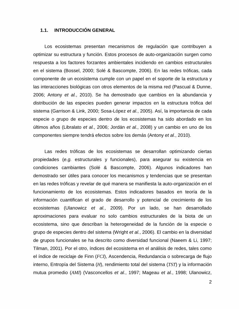
1.1. INTRODUCCIÓN GENERAL
Los ecosistemas presentan mecanismos de regulación que contribuyen a
optimizar su estructura y función. Estos procesos de auto-organización surgen como
respuesta a los factores forzantes ambientales incidiendo en cambios estructurales
en el sistema (Bossel, 2000; Solé & Bascompte, 2006). En las redes tróficas, cada
componente de un ecosistema cumple con un papel en el soporte de la estructura y
las interacciones biológicas con otros elementos de la misma red (Pascual & Dunne,
2006; Antony et al., 2010). Se ha demostrado que cambios en la abundancia y
distribución de las especies pueden generar impactos en la estructura trófica del
sistema (Garrison & Link, 2000; Sosa-López et al., 2005). Así, la importancia de cada
especie o grupo de especies dentro de los ecosistemas ha sido abordado en los
últimos años (Libralato et al., 2006; Jordán et al., 2008) y un cambio en uno de los
componentes siempre tendrá efectos sobre los demás (Antony et al., 2010).
Las redes tróficas de los ecosistemas se desarrollan optimizando ciertas
propiedades (e.g. estructurales y funcionales), para asegurar su existencia en
condiciones cambiantes (Solé & Bascompte, 2006). Algunos indicadores han
demostrado ser útiles para conocer los mecanismos y tendencias que se presentan
en las redes tróficas y revelar de qué manera se manifiesta la auto-organización en el
funcionamiento de los ecosistemas. Estos indicadores basados en teoría de la
información cuantifican el grado de desarrollo y potencial de crecimiento de los
ecosistemas (Ulanowicz et al., 2009). Por un lado, se han desarrollado
aproximaciones para evaluar no solo cambios estructurales de la biota de un
ecosistema, sino que describan la heterogeneidad de la función de la especie o
grupo de especies dentro del sistema (Wright et al., 2006). El cambio en la diversidad
de grupos funcionales se ha descrito como diversidad funcional (Naeem & Li, 1997;
Tilman, 2001). Por el otro, índices del ecosistema en el análisis de redes, tales como
el índice de reciclaje de Finn (FCI), Ascendencia, Redundancia o sobrecarga de flujo
interno, Entropía del Sistema (H), rendimiento total del sistema (TST) y la información
mutua promedio (AMI) (Vasconcellos et al., 1997; Mageau et al., 1998; Ulanowicz,

3
2001; Heymans et al., 2002; Heymans et al., 2007), han sido utilizados como
indicadores de la estabilidad del ecosistema y el estrés, que podrían otorgar
información valiosa sobre el papel de las especies. Estas evaluaciones se han
realizado conociendo que la reducción en biomasa de una especie o grupo de
especies que forman parte de la estructura de un ecosistema, sin duda afectará a las
relaciones en la red (Pauly et al., 2000).
El análisis del rol de las especies en el ecosistema se ha enfocado
principalmente en el uso de sus atributos morfológicos y ecológicos. En algunos
casos se ha llegado a conclusiones acerca de la pérdida de funciones relevantes en
el ecosistema, pero con débiles explicaciones de los procesos ecológicos inherentes
(Balvanera et al., 2006; Duffy, 2008). En este sentido, aún son insuficientes las
aproximaciones desde ese punto de vista y no existen evidencias de trabajos que
documenten el rol trófico de las especies que combinen el enfoque de la diversidad
funcional con el análisis de las especies en las redes tróficas. Esto debido a que a
menudo los modelos de ecosistemas no se desarrollan en la misma resolución que el
análisis de comunidades, es decir, en los modelos se analiza grupos funcionales
construidos a priori. El hecho de poderlos empatar y conjuntar, mostraría como
contribuye la variación temporal del rol de cada especie o grupo de especies dentro
de un ecosistema en los mecanismos de regulación, permitiendo detectar sí existen
ciertos atributos a nivel de especie que son relevantes en diferentes estados del
ecosistema.
En la Laguna de Términos se han presentado cambios en los patrones de
distribución y abundancias del necton, relacionados con actividades humanas y
variabilidad natural, que han modificado su estructura y procesos naturales (Ramos-
Miranda et al., 2005b). Así mismo, se han registrado cambios en las condiciones
ambientales de la laguna (Sirot et al., 2015). En consecuencia, se han evidenciado
también cambios tanto en la estructura trófica como en la diversidad taxonómica del
sistema lo que podría significar un cambio en el funcionamiento ecológico (Ramos-
Miranda et al., 2005a; Sosa-López et al., 2005), aunque estudios donde se evalúan el

4
tipo de locomoción y adquisición del alimento no han demostrado variaciones fuertes
a pesar de estos cambios en la composición específica (Villéger et al., 2008). Estas
variaciones hacen referencia a un patrón o arreglo espacial y temporal de los objetos
del sistema que responden al proceso de auto-organización (Camazine et al., 2003),
mecanismos que surgen como respuesta a perturbaciones que se manifiestan como
modificaciones en la topología y organización del ecosistema (Solé & Bascompte,
2006; Ulanowicz et al., 2009).
En este sentido, un análisis del rol de las especies en la estructura y
funcionamiento del ecosistema a partir de la diversidad funcional de las comunidades
biológicas y de indicadores relacionados con la función de cada especie o grupos de
especies podría explicar los mecanismos naturales que garantizan la tendencia
natural a la preservación y el orden del sistema. Por ejemplo, el rol que puede tener
una misma especie en el ecosistema puede ser cambiante de acuerdo a los cambios
en el ambiente. Por lo tanto, en este estudio se pretende utilizar diferentes enfoques
(diversidad funcional e índices de análisis de redes) a partir de datos biológico-
pesqueros colectados, modelos tróficos previamente publicados para la Laguna de
Términos y algunos de los atributos ecológicos de los grupos funcionales, para
analizar las funciones ecológicas de los grupos en el contexto de la preservación del
orden, estructura y funcionamiento del ecosistema en tres épocas diferentes en las
cuatro últimas décadas (1980, 1999 y 2011).
1.2. OBJETIVOS
1.2.1. General
Identificar y analizar las variaciones en el rol de las especies ícticas en los
procesos de auto-organización en el ecosistema de Laguna de Términos en el sur del
Golfo de México, y su relación con la variabilidad ambiental de la zona.
1.2.2. Específicos

5
1. Describir la variabilidad temporal de la diversidad funcional de las especies o
grupos de especies de la Laguna de Términos en el sur del Golfo de México.
2. Examinar la influencia de la variabilidad ambiental en los índices de diversidad
funcional y del ecosistema en la Laguna de Términos en el sur del Golfo de
México.
3. Identificar índices del ecosistema que permitan analizar y cuantificar
tendencias o patrones que expliquen los procesos de auto-organización en la
Laguna de Términos en el sur del Golfo de México de una estructura pasada a
la actual.
1.3. HIPÓTESIS
A menudo, cambios en el ambiente se traducen en variaciones en la
composición de las especies y diversidad, por lo que cambios temporales pueden dar
lugar a la selección de una nueva estructura. Se espera que en el ecosistema de la
Laguna de Términos presente cambios y que estos estén asociados a ciertos
indicadores de la red trófica, la diversidad y estructura funcional del ecosistema en
las últimas tres décadas, orientándose el ecosistema a un proceso de auto-
organización.
1.4. METODOLOGÍA GENERAL
1.4.1. Área de estudio
La Laguna de Términos es una laguna costera con condiciones estuarinas
ubicada en el sur del Golfo de México (Figura 1.1). Es la mayor laguna costera en
esta zona, con una superficie aproximada de 1.700 km2 en su cuenca principal y
2.500 km2 considerando los cuerpos de agua dulce adyacentes. Es una laguna
somera con una profundidad media de 3,5 m (Yañez-Arancibia & Day, 2005). Tiene
una alta diversidad de hábitats esenciales para la crianza y reproducción de muchas

6
especies (por ejemplo, pastos marinos, manglares, lechos de ostras, piscinas de
agua dulce, etc.; Manickchand-Heileman et al., 1998). Está delimitada en la
plataforma continental por una isla de barrera (Isla del Carmen) y conectada al mar
por dos bocas, Puerto Real en el este y El Carmen en el oeste. Las condiciones de
estuario de la laguna son producidas principalmente por los vertidos de tres ríos,
Palizada, Chumpan y Candelaria, con una media anual de descarga de 516 m3/s
(Yañez-Arancibia & Day, 2005).
Figura 1.1. Área de estudio. Los cuadros indican los puntos de muestreo para el periodo 1980/81 y los
círculos para los periodos 1998/99 y 2010/11.
La circulación del agua en la laguna sigue una dirección en el sentido de las
manecillas del reloj, con el flujo del agua de mar que entra a través de la boca de
“Puerto Real” y sale a través de la boca “El Carmen”. Existen tres temporadas
climáticas que se reconocen en la región: la estación seca (de febrero a mayo), la

7
temporada de lluvias (junio a septiembre) y la temporada de "nortes" (octubre a
febrero). Esta última se caracteriza por tormentas de invierno generadas por los
frentes fríos del norte con lluvias fuertes (hasta 1.850 mm/año) y vientos intensos (8
m/s) (Yáñez-Arancibia & Day, 1982; Yañez-Arancibia & Day, 2005). La temperatura
más alta se produce durante la temporada de lluvias, mientras que la temperatura
más baja se observa en la temporada de "nortes" (Yáñez-Arancibia & Day, 1982).
Dentro de La Laguna de Términos se han hecho investigaciones para distinguir
unidades ecológicas o subsistemas (Yáñez-Arancibia et al., 1982; Ramos-Miranda,
2000; Herrera-Silveira et al., 2002; Villalobos-Zapata et al., 2002). Sin embargo, no
ha sido fácil establecer límites espaciales y temporales debido a la alta variabilidad
ambiental del área. Durante estas investigaciones se han descrito los sistemas
hidroecológicos, evidenciando una gran variación en los últimos años, esto con el
objeto de describir aquellos mecanismos de adaptación que desarrollan las
comunidades de peces en sus ciclos de vida de acuerdo a la variabilidad ambiental
de la zona (Sosa-Lopez, 2005). Así, se han identificado unidades ecológicas
espaciales —la cuenca central de la laguna, la zona de influencia de la descarga de
los ríos, las bocas oceánicas y la parte interna de la isla del Carmen—, pero, debido
a la variabilidad ambiental, ha sido difícil establecer un patrón. Estas unidades sin
límites bien definidos, muestran la hidrología y sedimentología de la laguna (Villéger
et al., 2010). Por ejemplo, la zona de la boca “El Carmen” recibe una marcada
influencia del río Palizada, por lo que presenta un amplio rango de salinidad y su
sustrato está compuesto por barro con arena fina y limo arcilloso. La zona de Isla del
Carmen y la boca “Puerto Real” tiene influencia marina (salinidad en promedio de
28.5 UPS) y el sustrato presenta desde áreas lodosas junto a los manglares hasta
zonas arenosas donde habitan pastos marinos. La zona correspondiente a la parte
sur de la laguna es la más somera, con sustrato limo-arcilloso y gran cantidad de
zonas de manglares, recibe la mayor influencia de las descargas de los ríos
Chumpan y el sistema Candelaria-Mamantel. El centro de la laguna, que presenta las
mayores profundidades, es una zona transicional entre el ambiente marino y el que
recibe descargas de aguas continentales (Villéger et al., 2010).

8
La cobertura de manglares ha sufrido reducciones, pero se ha observado una
aparente recuperación desde 1991 hasta 2001, sin embargo esta zona alcanza sólo
el 70% del nivel alcanzado en 1974. En contraste, la cobertura agrícola se
incrementó un 300% desde 1974 hasta 1991 (Sosa-Lopez, 2005). En este mismo
sentido, los insumos contaminantes de la agricultura y la pérdida de hábitats debido a
la deforestación podrían afectar no sólo a la estructura y la abundancia de las
comunidades de peces sino también la funcionalidad del ecosistema (Ramos-
Miranda et al., 2005a; Villéger et al., 2010; Galeana-Cortazar, 2015). En términos de
la estructura trófica de la laguna, se ha evidenciado cambios temporales entre los
periodos 1980/81 y 1998/99, mostrando que la biomasa de las especies omnívoras
(especies estuarinas de la parte media de la red trófica), ha sido reemplazada por
especies carnívoras y herbívoras-detritívoras (niveles tróficos altos y bajos,
respectivamente) (Sosa-López et al., 2005). Estos cambios evidentes también
podrían conducir a una pérdida en la capacidad de respuesta ecológica a las
fluctuaciones ambientales y un cambio en el funcionamiento ecológico.
Villéger et al. (2010) en un estudio realizado sobre la evaluación de atributos
como la locomoción y adquisición de alimento de los peces, señalaron que no existen
cambios en gran parte de la laguna, a pesar de que la composición específica si ha
cambiado. Por otro lado, en el análisis de la comparación de la red trófica de la
laguna, se han detectado cambios funcionales más no estructurales, donde se ha
evidenciado una tendencia negativa en la magnitud de flujos de energía totales entre
los periodos 1980/81, 1998/99 y 2010/11, pero los grupos de mayor cohesión y
conectividad en el ecosistema se han mantenido relativamente estables con el paso
del tiempo (Abascal-Monroy, 2013). Estos resultados sugieren la existencia de ciertos
procesos de auto-organización o estabilidad en la laguna.
1.4.2. Procedencia de los datos

9
Tres seguimientos biológicos mensuales se llevaron a cabo en la laguna en
diferentes décadas: febrero 1980 a enero 1981, febrero 1998 a enero 1999 y
noviembre de 2010 a octubre de 2011. Durante los tres seguimientos fueron
muestreados los mismos sitios (17 estaciones de muestreo) (Figura 1.1) y se
utilizaron artes de pesca similares (red de arrastre de 2.5 m de abertura de trabajo
óptima y 19 mm tamaño de malla) con arrastres de 12 min a 2,5 nudos de velocidad.
Se ha descrito que este arte de muestreo es apropiado por ser una zona costera
poco profunda y las especies presentes que viven en el área son relativamente
pequeñas y nadadores regulares (Villéger et al., 2010). La composición (número de
especies) y abundancia de las especies de peces (en número de individuos y
biomasa de la captura) se registraron en cada estación de muestreo. Las especies
fueron identificadas hasta el más bajo nivel taxonómico posible utilizando las claves
especializadas de identificación. Asimismo, seis variables ambientales se registraron
en cada estación de muestreo: profundidad y transparencia, además de la
temperatura y salinidad de superficie y fondo (para más detalles de los muestreos ver
Ramos-Miranda et al., 2005a; Villéger et al., 2010).
La información colectada ha permitido construir modelos tróficos para estos
periodos (para 1980: Manickchand-Heileman et al., 1998; Zetina-Rejón, 2004; para
1998 y 2011: Abascal-Monroy, 2013). Estos modelos consideran en general 40
grupos funcionales: 25 de peces, nueve de invertebrados (jaibas, camarón blanco,
camarón café, camarón rosado, moluscos, equinodermos, microcrustáceos,
poliquetos, meiobentos), dos de productores primarios (fitoplancton y zooplancton),
uno de detritus y uno para mamíferos marinos (defines), así como para reptiles
(tortugas marinas) y aves marinas (Abascal-Monroy, 2013).
1.4.3. Análisis de los datos
El análisis del rol de las especies o grupos de especies se realizó a partir de
dos enfoques para cada una de las tres épocas (1980, 1999 y 2011). En el primero,
con la información biológico-pesquera colectada para cada periodo, se efectuó un

10
análisis de la diversidad funcional haciendo una compilación de datos sobre la
historia de vida y características ecológicas (rasgos funcionales) de cada especie. El
segundo enfoque consistió en evaluar el papel de cada especie o grupo de especies
en el ecosistema a partir de indicadores basados en la teoría de la información
propuesta por Ulanowicz (1986); ambos enfoques se detallan a continuación:
1.4.3.1. Análisis de diversidad funcional
Para el análisis de diversidad funcional se seleccionaron atributos ecológicos y
morfológicos de las especies con base en los criterios de diversos autores (Dumay et
al., 2004; Álvarez-Filip & Reyes-Bonilla, 2006; Gristina et al., 2006; Palacios-Salgado,
2011, entre otros). Los atributos ecológicos y morfológicos que se consideraron
fueron: nivel trófico, gremio trófico, gremio reproductivo, hábitat, uso de estuarios,
hábitat esencial, tolerancia a la salinidad, forma del cuerpo, aleta caudal, tipo de boca
y longitud máxima reportada. El análisis de diversidad funcional se basó en describir
el rango, distribución y abundancia de los rasgos funcionales en el ecosistema
relacionados con la función ecológica de las especies (Schleuter et al., 2010). Con el
uso de estos rasgos se ha demostrado que la diversidad funcional depende de su
distribución y no del número de especies (Mason et al., 2003)
1.4.3.2. Análisis del rol funcional
A partir de los modelos tróficos, se utilizó la matriz de los flujos de consumo (la
cual representa la red trófica del ecosistema lagunar). Esta matriz fue útil para
calcular los índices respecto al funcionamiento de los ecosistemas a partir de la
teoría de la información relacionados con el concepto de ascendencia de Ulanowicz
(1986), que es un indicador del crecimiento y desarrollo del ecosistema y mide la
organización de la red trófica.

2. ANÁLISIS TEMPORAL DE LA DIVERSIDAD FUNCIONAL

12
2.1. Cambios temporales en las características funcionales de la
comunidad de peces en la Laguna de Términos en tres periodos
(1980, 1998 y 2011)
2.1.1. Introducción
En ecología, existen tres enfoques diferentes para la evaluación de la
diversidad en las comunidades y los ecosistemas biológicos: descriptivo, funcional y
evolutivo. El enfoque descriptivo se orienta en medir la diversidad en la composición
de especies y distribución de la abundancia. El enfoque evolutivo tiene en cuenta el
número de especies y su relación filogenética. El enfoque funcional considera la
variedad de rasgos funcionales de las especies. Los tres enfoques dependen de la
distribución y abundancia, así como de la diversidad y la variedad de características
funcionales que los caracterizan (Wright et al., 2006). Aunque el enfoque descriptivo
y evolutivo se han utilizado como indicadores potenciales del funcionamiento de los
ecosistemas, las especies estrechamente relacionadas filogenéticamente no siempre
realizan funciones similares y, por el contrario, especies poco vinculadas pueden
tener funciones similares en el apoyo y el funcionamiento del ecosistema (Botta-
Dukát, 2005; Lombarte et al., 2012). Por esta razón, cuando se consideran los rasgos
funcionales de las especies, es útil tener en cuenta la diversidad de las funciones de
las especies en un ecosistema. Por ejemplo, si un ecosistema tiene un alto número
de especies redundantes, es decir, las especies poseen funciones similares,
deberían ser menos vulnerables a las perturbaciones. En este sentido, comprender la
diversidad funcional sobre una base temporal es importante para detectar los
cambios que pueden comprometer el funcionamiento de los ecosistemas. Además, la
gestión basada en los ecosistemas se está adoptando como principio rector en el
manejo, por lo que una mayor comprensión de la estructura y funcionamiento de los
ecosistemas marinos es esencial (Huse, 2012).
Así, en los últimos años, los enfoques para la simplificación de la complejidad
de los ecosistemas, como los que evalúan la funcionalidad del ecosistema, han

13
aumentado (Mouillot et al., 2011). La diversidad de los rasgos funcionales de un
ecosistema puede describir y explicar los procesos inherentes a su funcionamiento,
revelar los procesos que intervienen en la estructuración de la comunidad (Villéger et
al., 2012) e indicar las diferencias en las respuestas ecológicas a las perturbaciones
(Lombarte et al., 2012). Sin embargo, la diversidad funcional no siempre es fácil de
medir porque no hay ninguna medida estandarizada y se carece de índices que
simplifiquen esta complejidad (Somerfield et al., 2008; Villéger et al., 2010).
Las comunidades están sometidas a perturbaciones bióticas y abióticas que
modifican su estructura (Lombarte et al., 2012), por lo que es necesario conocer
además su relación con la variabilidad ambiental. En este sentido, no sólo es
importante conocer la variedad y complejidad de rasgos funcionales que forman parte
del funcionamiento de los ecosistemas, sino también las condiciones y
perturbaciones ambientales que a través del tiempo pueden influir en la estructura
funcional (Dale & Beyeler, 2001). La evaluación de la respuesta de las comunidades
a la variabilidad ambiental para describir los patrones de biodiversidad en el proceso
de los ecosistemas se ha centrado en el análisis de los cambios a nivel de especies,
y muy poco en las características funcionales que podrían estar influyendo en los
procesos (Casanoves et al., 2011; Buisson et al., 2013). Particularmente, en el caso
de las comunidades de peces en los estuarios tropicales, que tienen una amplia
gama de rasgos morfológicos y ecológicos que influyen en los procesos de los
ecosistemas, el cambio constante de la estructura de la comunidad en el espacio y el
tiempo podría revelar cambios a nivel de ecosistemas (Villéger et al., 2011).
La dinámica del ecosistema costero lagunar, Laguna de Términos (Figura 1.1),
se ve afectada por múltiples causas, principalmente de origen antrópico. Estas
afectaciones incluyen: la industria del petróleo y la pesca comercial en la plataforma
continental adyacente, crecimiento de la población en los asentamientos urbanos
existentes, cambios en el uso del suelo, deforestación de los manglares y
humedales, desarrollo agrícola y ganadero y los cambios en las condiciones
hidrológicas de la laguna por el represamiento y uso de los ríos que la alimentan, que

14
constantemente cambian la salinidad (Ramos-Miranda et al., 2005a; Sosa-López et
al., 2005). Además, las actividades humanas y la variabilidad ambiental han
modificado la estructura y los procesos naturales, particularmente en los patrones de
distribución y abundancia de necton (Ramos-Miranda et al., 2005a; Sirot et al., 2015).
Así mismo, los cambios tanto en la estructura trófica y la diversidad taxonómica del
sistema son evidentes y pueden conducir a la pérdida de la capacidad de respuesta
ecológica a las fluctuaciones ambientales y la pérdida en el funcionamiento ecológico
(Ramos-Miranda et al., 2005a; Sosa-López et al., 2005). Sin embargo, Villéger et al.
(2010) realizaron una comparación temporal de las comunidades de peces entre
1980 y 1998, llegando a la conclusión que la laguna no mostró fuertes cambios
funcionales en el grado de especialización funcional de las especies. Igualmente,
destacaron el aumento de especies redundantes y la disminución de las especies
con rasgos funcionales especializadas vinculadas a los hábitats de pastos marinos.
No obstante, los investigadores identificaron la necesidad de un enfoque multifacético
en la evaluación de los cambios en las comunidades.
Los rasgos responsables del funcionamiento de un ecosistema en particular
dependen de numerosos factores, incluyendo las condiciones de temperatura, el
suelo, el agua, la lluvia, y la disponibilidad de nutrientes. En muchos casos, las
características importantes en la determinación de una función de determinado
ecosistema se pueden compartir entre múltiples especies en un conjunto. La Laguna
de Términos ha sido declarada un hábitat crítico para los peces en las primeras
etapas de la vida, por lo que se han implementado algunas medidas de seguridad
para la conservación de los peces (Área de Protección de Flora y Fauna en 1994 y
sitio Ramsar en 2004) las cuales podrían influir en los cambios no sólo en la
estructura, sino también en el funcionamiento de los ecosistemas a través del tiempo.
En las últimas tres décadas, la laguna ha sido sometida a diversas perturbaciones
que pueden afectar no sólo la estructura de los ecosistemas, sino también la
diversidad funcional, que puede dar lugar a diferentes respuestas ecológicas. Por lo
tanto, el objetivo de esta parte del estudio fue evaluar los cambios en los patrones
temporales de la estructura funcional de las comunidades de peces entre los años

15
1980, 1998 y 2011. Estos cambios se evaluaron utilizando un nuevo índice de
diversidad funcional que tiene en cuenta los datos morfológicos y ecológicos así
como la biomasa de cada especie y/o los rasgos funcionales de la comunidad de
peces. Finalmente, se describe la relación de la estructura funcional con la
variabilidad ambiental del ecosistema.
2.1.2. Análisis de los datos
Para cada una de las especies de peces se seleccionaron los rasgos de historia
de vida y ecológicos que eran sensibles a la degradación del hábitat (es decir, los
cambios en la estructura trófica, los cambios en la salinidad, la pérdida de hábitats
críticos, gremios reproductivos dominantes, hábitat esenciales) (Wainwright et al.,
2002; Goldstein & Meador, 2005; Villéger et al., 2010). Los rasgos de la historia de
vida y ecológicos para cada especie fueron recopilados utilizando una variedad de
fuentes, incluidos los registros para el área de estudio, catálogos de especies, libros
y la base de datos Fishbase® (www.fishbase.org). Los rasgos funcionales
seleccionados podrían ser datos continuos o categóricos; por lo tanto, todos fueron
categorizados para hacerlos comparables (Tabla 2.1).
2.1.2.1. Índice de diversidad de atributos funcionales
Para simplificar la estructura funcional de la comunidad de peces, se desarrolló
un nuevo índice denominado Índice de Diversidad de Atributos Funcionales (FADI
por su sigla en inglés, Functional Attribute Diversity Index). Este índice tiene en
cuenta la probabilidad de obtener una especie con determinado atributo funcional
particular (i) entre todos los demás. Por ejemplo, de un total de 128 especies en el
área, 26 de ellas posee un nivel trófico >4,01, la probabilidad de ocurrencia de este
atributo está dada por la relación 26/128 = 0,202 (Tabla 2.1). Se denominó a esta
probabilidad como redundancia (R) debido a que un valor cercano a uno indicaría la
existencia de muchas especies con este atributo y valores cercanos a cero indicaría
una baja incidencia de especies con el mismo atributo. En este sentido, rasgos

16
menos redundantes podrían ser más importantes para la diversidad funcional, ya que
procesos ecológicos particulares o funciones de los ecosistemas podrían depender
de algunas especies. Una menor redundancia implicará una mayor diversidad; por lo
tanto, para dar mayor importancia a los rasgos menos redundantes, este valor se
transformó como (1 - R) lo que representa el valor funcional (FV) del atributo por
especie.
El FADI tuvo en cuenta el FV ponderado por la abundancia relativa de las
especies y la formulación matemática es:
donde S es el número de especies, n es el número de rasgos, Bi es la biomasa
de la especie i y B es la biomasa total. Se calculó un valor de FADI para cada uno de
los tres períodos estudiados para evaluar los cambios temporales. Del mismo modo,
se calcularon los valores FADI para cada mes dentro de los tres períodos estudiados
y para cada una de las estaciones climáticas para analizar la variación intra-anual de
los valores de la diversidad funcional.
Los valores FADI no pueden ser estrictamente comparados, ya que las
comunidades de peces tienen diferentes números de especies y diferentes biomasas
entre los tres períodos. Sin embargo, para la comparación de los valores de FADI, se
calculó una distribución de probabilidad del índice en un remuestreo bootstrap (1000
muestras), asumiendo un modelo nulo que indica la coexistencia de los peces de
forma azarosa en la Laguna. Básicamente, en este proceso, las especies fueron
seleccionadas al azar de una por una hasta el número total de especies reportadas
para los tres períodos (n = 128). El valor funcional de las especies seleccionadas se
dividió por el número de especie “re-muestredas”, suponiendo abundancias iguales
(distribuidos por igual en las n especies) entre las especies seleccionadas para
estimar los valores de FADI en cada paso. Esta distribución de los valores nulos fue
utilizada para producir distribuciones de probabilidad del 95%, que luego se
𝐹𝐴𝐷𝐼 =∑ [(∑ 𝐹𝑉𝑙
𝑛𝑙=1 ) ×
𝐵𝑖
𝐵 ]𝑆𝑖=1
𝑛

17
representaron frente a los valores observados del FADI para los tres periodos. De
este modo, se probó si los valores FADI para cada año fueron significativamente
diferentes de los valores esperados por azar.
Tabla 2.1. Rasgos funcionales utilizados para el cálculo de FADI. Se muestran las categorías y
los valores de redundancia (R) dada por la relación del número de especies de atributo (i) entre el
número total de especies (n = 128).
Rasgo (i)
Categorías R Rasgo
(i) Categorías R
Ale
ta C
aud
al
Redondeada 0,17
Niv
el T
rófico
< 2,50 0,05
Truncada 0,12 2,51 – 3,00 0,04
Emarginada 0,05 3,01 – 3,50 0,30
Semilunada 0,04 3,51 – 4,00 0,41
Ahorquillada 0,41 > 4,00 0,19
Confluente 0,04
Gre
mio
Repro
ductivo
Ovíparos con gestación oral 0,03
Punteada 0,05 Ovíparos huevos bentónicos y fase pelágica 0,04
En forma de “S” 0,02 Ovíparos huevos bentónicos y sin fase pelágica 0,03
Doble emarginada 0,03 Ovíparos huevos pelágicos 0,81
Sin caudal 0,05 Ovovivíparos 0,09
Elasmobranquios 0,02
Gre
mio
Tró
fico
Carnívoros Ictio-Invertívoros 0,33
Form
a d
el C
uerp
o
Alargado 0,05 Carnívoros Piscívoros 0,53
Comprimido Lateral 0,56 Carnívoros Invertívoros 0,02
Comprimido Ventral-A 0,12 Omnívoros 0,08
Comprimido Ventral-B 0,10 Planctívoros 0,05
Fusiforme 0,03
Hábitat
Pelágico 0,13
Globo 0,09 Bentopelágico 0,18
Sagitiforme 0,04 Demersal fondos blandos 0,26
Teniforme 0,01 Demersal fondos duros 0,02
Otras formas 0,01 Demersal fondos mixtos 0,27
Bentónico 0,14

18
Rasgo (i)
Categorías R Rasgo
(i) Categorías R
Tip
o d
e B
oca
Oblicua 0,01
Uso d
e E
stu
ari
os
Agua Dulce 0,01
Superior 0,03 Marino 0,35
Terminal 0,28 Marino-Anfídromo 0,52
Inferior 0,16 Agua Dulce-Anfídromo 0,02
Ventral 0,05 Anádromo 0,01
Protáctil 0,09 Oceanódromo 0,08
Tubular 0,04 Catádromos 0,02
Incluida 0,02
Hábitat
Esencia
l
Pastos Marinos 0,16
Proyectante 0,30 Algas 0,07
Semiventral 0,03 Arena 0,07
Tole
rancia
a
la S
alin
idad
Estenohalino 0,34 Arena-Lodo 0,51
Eurihalino 0,47 Grava-Arena 0,03
Eurihalino+ 0,19 Lodo 0,03
Long
itu
d
Máxim
a < 300 mm 0,29 Manglares 0,12
301 - 600 mm 0,41
> 600 mm 0,30
2.1.2.2. Análisis Multivariado
Se utilizó un análisis de ordenación (Escalamiento Multidimensional no Métrico -
MDS) para explorar las variaciones similares de los rasgos funcionales o las
variables ambientales. El MDS se realizó utilizando la distancia Euclidiana como
medida de similitud a partir de los valores medios mensuales estandarizados de las
variables ambientales y el valor funcional (FV) de cada rasgo ponderado por la
biomasa relativa. El MDS representó los rasgos funcionales y las variables
ambientales en un espacio de dos dimensiones, de tal manera que las distancias
relativas entre todos los puntos estaban en el mismo orden de rango. Las variables
ambientales o los rasgos funcionales que estaban cerca uno del otro eran más
similares que los que estaban distantes unos de otros. Este análisis nos permitió
seleccionar los rasgos funcionales y las variables ambientales que no eran similares

19
para realizar un análisis de componentes principales (PCA) para resumir la
información de los rasgos funcionales e identificar la contribución relativa de ellos a la
varianza total de la diversidad funcional. Sólo los componentes principales con
valores superiores a uno fueron retenidos, y la contribución de los rasgos funcionales
a la varianza explicada de PC se cuantificó. Además, se proyectaron las variables
ambientales en el espacio generado por los dos componentes principales para fines
de interpretación.
2.1.3. Resultados
Un total de 128 especies fueron registradas durante las tres campañas. Los
valores de redundancia de cada rasgo funcional se muestran en la Tabla 2.1. Los
valores medios del FADI para los tres años (0,708, 0,716 y 0,690 para 1980, 1998 y
2011, respectivamente) mostraron diferencias significativas (F(2,33)=24,732; p = 0,000)
(Figura 2.1a). Se contrastaron estos valores con la distribución de probabilidad
producida por el modelo nulo y puso de manifiesto que el valor del FADI para 1998
estuvo por fuera del límite superior de la distribución esperada. Este resultado indica
una mayor presencia de especies con alto valor funcional o con menos rasgos
funcionales redundantes. En general, los valores de FADI para 1998 (mensuales y
estacionales) cayeron fuera del límite superior de la distribución esperada (Figura
2.1b y Figura 2.1c). Para las otras dos campañas, los valores de FADI estaban
dentro de la distribución prevista de probabilidad. La tendencia de 2011 mostró
valores más homogéneos, lo que indica que la biomasa por atributo funcional se
distribuyó uniformemente.
El análisis de ordenación (Figura 2.2) mostró las similitudes entre los rasgos y
las variables ambientales con un nivel de estrés de 0,17, una representación
potencialmente adecuada (Clarke & Warwick, 2001). En relación a los rasgos
funcionales, se encontró que no existía similitud entre ellos porque estaban muy
separados en el espacio de ordenación.

20
Figura 2.1. Valores del FADI para: (a) promedio anual, (b) media por época y (d) promedio mensual.
Colores en los símbolos representan los tres períodos evaluados: negro=1980, gris=1998 y
blanco=2011. Se muestra la distribución de probabilidad del 95% y el valor medio para el número de
especies. Esta distribución se realizó con un remuestreo bootstrap (1000 muestras).

21
Figura 2.2. Ordenación (MDS) de los rasgos funcionales (negrita) y las variables ambientales (cursiva).
TL=Nivel Trófico, RG=Gremio Reproductivo, TG=Gremio Trófico, BS=Forma del Cuerpo, MT=Tipo de
Boca, CF=Aleta Caudal, ML=Longitud Máxima, HA=Hábitat, UE=Uso de Estuarios, EH=Hábitat
Esencial, ST=Tolerancia a la Salinidad, DEP=Profundidad, TRA=Transparencia, SST=Temperatura
Superficial, BST=Temperatura del Fondo, SSS=Salinidad superficial y BSS=Salinidad del Fondo.
Para las variables ambientales, la salinidad y la temperatura de superficie y
fondo presentaron comportamientos semejantes en la representación del MDS lo que
indica una alta similitud, razón por la que los valores del fondo no fueron
considerados en la interpretación de los análisis de PCA (Figura 2.2).
Usando los rasgos funcionales seleccionados, los tres primeros componentes
del análisis PCA explicaron el 81.75% de la varianza total (PC1 = 33,75%, PC2 =
31,77% y PC3 = 16,23%). Se identificaron dos grupos principales, un grupo formado
por los períodos 1980 y 2011 y el otro grupo formado por el período de 1998 (Figura
2.3). Para los valores de 1998, 10 de las 12 muestras fueron ordenadas en el
cuadrante superior derecho. Los otros dos períodos fueron ordenados en los otros
cuadrantes, destacando que más de 60% de las muestras de 1980 estaban en el
cuadrante superior izquierdo, y todas las muestras del 2011 en los cuadrantes
inferiores (Figura 2.3). La ordenación de los rasgos funcionales mostró las más altas
(>0,5) correlaciones del primer componente con los rasgos morfológicos (forma del
cuerpo, forma de la boca y la aleta caudal), así como el nivel trófico y hábitat. El

22
segundo componente tenía las más altas correlaciones con los rasgos ecológicos
(gremio reproductivo, uso de estuario, hábitat esencial, de hábitat, y tolerancia a la
salinidad; Tabla 2.2). La variabilidad ambiental mostró la profundidad como la
variable con la mayor correlación con los dos primeros componentes (Figura 2.3).
Figura 2.3. Ordenación de Componentes Principales de los rasgos funcionales (línea continua) de
cada mes en los tres períodos analizados. Colores del símbolo representan los tres períodos
evaluados: negro: 1980, gris: 1998 y blanca: 2011. TL = Nivel Trófico, RG = Gremio Reproductivo, TG
= Gremio Trófico, BS = Forma del Cuerpo, MT = Tipo de Boca, CF = Aleta Caudal, ML = Longitud
Máxima, HA = Hábitat, UE = Uso de Estuarios, EH = Hábitat Esencial, y ST = Tolerancia a la
Salinidad. Además, las variables ambientales (línea punteada) se proyectan para fines de
interpretación. DEP = Profundidad, TRA = Transparencia, SST = Temperatura Superficial, y SSS =
salinidad superficial.

23
Tabla 2.2. Correlaciones entre los rasgos funcionales y los tres primeros componentes principales que
explican el mayor porcentaje de la varianza.
Variable PC 1 PC 2 PC 3
TL 0.91 -0.23 0.09
RG -0.11 0.92 -0.09
TG 0.35 0.08 -0.17
BS -0.94 0.19 -0.12
MT 0.62 0.16 0.66
CF -0.83 -0.25 0.38
ML -0.05 0.91 0.24
HA -0.72 0.53 0.26
UE 0.27 0.86 -0.26
EH 0.18 0.37 -0.87
ST 0.42 0.69 0.45
2.1.4. Discusión
Las tres facetas de índices de diversidad funcional han demostrado ser
independientes de la riqueza y la equidad de las especies. Los índices que utilizan
caracteres individuales y múltiples para identificar rasgos que están específicamente
relacionados con el funcionamiento de los ecosistemas han aumentado en los
últimos años (Mason et al., 2005). El FADI utiliza múltiples atributos en el mismo
análisis, lo que ayuda a inferir estrategias ecológicas y examinar la relación entre la
riqueza de especies y la diversidad funcional (Flynn et al., 2009). Además, la
combinación de múltiples rasgos funcionales puede ayudar a detectar la influencia de
la variabilidad ambiental en la funcionalidad del ecosistema.
La comunidad de peces de las lagunas costeras está sujeta a variaciones
ambientales, que con el tiempo influyen en su composición y, de esta manera,
aumentan o disminuyen la riqueza de especies. Sin embargo, es posible que se vean
afectados en términos del valor biológico de sus rasgos ecológicos y morfológicos
(diversidad funcional) (Botta-Dukát, 2005; Villéger et al., 2012). Por el contrario, el
FADI fue capaz de detectar una variabilidad temporal que puede estar influenciada
por las variables ambientales, principalmente por la profundidad, lo que está
24
relacionado con la varianza explicada de los rasgos funcionales del PC1 y PC2.
Ramos-Miranda et al. (2005a) determinaron que, durante el año 1998, la Laguna de
Términos fue menos profunda, con una mayor transparencia y mayor salinidad, lo
que podría estar relacionado con las abundancias más altas de depredadores de
altos niveles tróficos y afinidad marina como visitantes ocasionales en la laguna. Este
hecho podría estar asociado con cambios en la estructura funcional de las
comunidades biológicas de la laguna. Por ejemplo, el nivel trófico tuvo la mayor
correlación con el PC1. Además, se encontró una variación consistente en la
biomasa de diferentes niveles tróficos en el tiempo, según lo sugerido por Sosa-
López et al. (2005).
Por el contrario, durante los períodos de 1980 y 2011, las condiciones
estuarinas favorecieron la presencia de especies de niveles tróficos intermedios
(Sosa-López et al., 2005). Estos cambios ambientales también condujeron a una
mayor variabilidad taxonómica (Ramos-Miranda et al., 2005a) y de las estructuras
funcionales (este estudio). La mayor variabilidad funcional que se encuentra en los
niveles tróficos de la comunidad de peces también podría estar relacionada con la
pérdida de hábitats críticos que sirvieron como áreas de cría para especies de
niveles tróficos bajos o juveniles de altos niveles tróficos (Lombarte et al., 2012). Una
ligera recuperación de los manglares hacia principios de la década de 2000, en
comparación con la década de 1990, aunque por debajo de la cantidad existente en
la década de 1980 (Sosa-Lopez, 2005), podría explicar por qué la diversidad
funcional fue mayor durante 1998.
Por otra parte, la variabilidad ambiental indujo una respuesta diferente en las
estrategias funcionales o una asociación entre la abundancia de las especies y los
rasgos funcionales medidos (Ramos-Miranda et al., 2005a; Villéger et al., 2012). Esto
último es lo que ocurrió en la laguna, por lo que no es posible sugerir que la pérdida
de un atributo funcional afectaría al funcionamiento del ecosistema (Villéger et al.,
2010; Lombarte et al., 2012). Se ha sugerido que la declaración de la Laguna de
Términos como un área protegida en el año 2004 ha influido en la reorganización de

25
la laguna (Abascal-Monroy et al., 2015) pero aún evidencia contundente dado que
por el persistente y continuo crecimiento urbano, la pesca ilícita y la industria. Sin
embargo, Sirot et al. (2015) han sugerido que las condiciones ambientales de la
laguna, en especial si se miran la variables pH, profundidad y transparencia, afectan
la dominancia de algunas especies y cuyos valores registrados fueron muy similares
entre 1980 y 2011. Este hecho influiría en la gran similitud de los valores de FADI
entre estos dos años, dado que estas variables afectan a un mayor número de
especies que la misma salinidad y temperatura (Sirot et al., 2015). Estos autores
también destacan el hecho que una de las variables ambientales de mayor influencia
en la estructura de la laguna sea la profundidad, lo que coincide con los resultados
de este estudio, como la variable más influyente en la diferencias en el análisis
temporal de la diversidad funcional. La evidencia generada en este estudio apoya la
idea de una reestructuración funcional de la comunidad de peces.
Los diferentes enfoques para evaluar la funcionalidad de una comunidad se han
centrado en el uso de una amplia gama de índices de diversidad funcional. Algunos
de estos índices se basan en la topología de un análisis de conglomerados o las
ramas de las distancias genéticas de la especie, y algunos son ponderados por la
biomasa relativa de la especie, pero pocos han utilizado muchos rasgos a la vez
(Botta-Dukát, 2005). Aunque los índices de diversidad funcional están limitados en su
aplicación, se sugiere que el uso combinado de datos categóricos y continuos en los
cálculos de los índices de las variables de diversidad funcional no son del todo
correcto, pero hay maneras de usarlos realizando transformaciones a la variables
categóricas en variables continuas (Schleuter et al., 2010), como se hizo en el diseño
del FADI. Aunque la realización de este tipo de transformación podría dar lugar a una
cierta pérdida de información (Schleuter et al., 2010), este enfoque nos ha permitido
incorporar múltiples rasgos funcionales en un solo índice de la estructura funcional de
un ecosistema.
El uso de múltiples rasgos funcionales en la evaluación de la funcionalidad de
los ecosistemas podría ayudar a clarificar la respuesta de la comunidad a diversos

26
procesos que pueden ocurrir en el ecosistema y examinar la relación entre la riqueza
de especies y la diversidad funcional de la comunidad (Flynn et al., 2009). Por lo
tanto, es importante incluir variables y/o rasgos funcionales de diferentes tipos que
pueden describir la funcionalidad del ecosistema, independientemente de sus
características (Cornwell et al., 2006). A la fecha no existe un estándar de cuántos y
cuáles rasgos hay que usar para calcular la diversidad funcional, sin embargo este
índice ha sido diseñado para ser ponderado por el número de rasgos funcionales que
se usen, y su fortaleza radica en la valoración de los rasgos menos comunes o
redundantes. El uso de muchas especies y muchos rasgos funcionales mostró
mejores resultados que usando pocas especies y rasgos funcionales, lo que fue
confirmado mediante el uso de índices taxonómicos, niveles tróficos y redes tróficas,
y podría maximizar diferentes propiedades del ecosistema (Schleuter et al., 2010).
La selección de los rasgos funcionales y el número necesario para evaluar la
diversidad funcional de una comunidad es uno de los retos en la medición de la
diversidad funcional. Actualmente, como se ha mencionado, no existe un acuerdo
sobre las características que se deben tener en cuenta para seleccionar los rasgos
útiles para medir la diversidad funcional, sólo se hace énfasis en que estas
características deban ser medibles. Es importante destacar que es estrictamente
necesario que el número de especies deba ser mayor que el número de rasgos
funcionales evaluados. Con este enfoque, se ha podido discriminar las variaciones
temporales en la diversidad funcional de los ecosistemas que cambian
constantemente debido a las altas fluctuaciones de las condiciones ambientales.
Recientemente, en la evaluación de la diversidad funcional se ha incluido la
ponderación por la abundancia de los rasgos funcionales de las especies (Schleuter
et al., 2010). Como resultado de esta ponderación, la diversidad funcional se ha
dividido en tres tipos de medición que evalúan las diferentes facetas de la diversidad
funcional: riqueza, equidad y divergencia. La riqueza funcional mide cómo existen
muchos atributos funcionales en un espacio o nicho determinado. La equidad
funcional y divergencia funcional miden la distribución y el grado de la abundancia en

27
este nicho, respectivamente, dentro de la comunidad (Schleuter et al., 2010). Las tres
facetas miden diferentes aspectos de la diversidad funcional y por lo tanto podrían
ser independientes entre sí con respecto a varios rasgos o caracteres funcionales
(Schleuter et al., 2010). Debido a que el FADI pondera el valor funcional de cada
especie por su abundancia, se puede indicar que el índice evalúa la segunda faceta
que se ha descrito anteriormente, midiendo el grado de distribución de la abundancia
en los rasgos funcionales.
Como la diversidad funcional consiste en la riqueza y frecuencia de los rasgos
morfológicos y fisiológicos fundamentales, las comunidades con un alto número de
especies, pero diversidad funcional baja, puede decirse que tienen alta "redundancia
funcional" (Petchey et al., 2007; Flynn et al., 2009). La alta redundancia funcional se
produce cuando las especies se solapan en sus rasgos, lo que puede reflejar
solapamiento de nicho si los rasgos se definen de una manera biológicamente
apropiada (Flynn et al., 2009). El FADI muestra redundancia funcional cuando los
valores están fuera de la distribución de probabilidad. En otras palabras, cuando los
valores estuvieron por debajo de la distribución, la estructura funcional fue dominada
por especies con los rasgos redundantes, y cuando los valores estaban por encima
de la distribución, la estructura funcional fue dominada por especies con rasgos
menos comunes. En 1998, se encontró una mayor redundancia dada por la alta
biomasa de rasgos funcionales menos comunes, mientras que para los otros dos
periodos, los valores se mantuvieron dentro de la distribución de probabilidad
indicando mayor equidad funcional.
En muchos casos, la diversidad ecológica ha sido relacionada y utilizada como
un indicador importante de la función del ecosistema (Tilman et al., 1997; Hooper et
al., 2002), ya que los cambios en la diversidad, distribución y abundancia espacio-
temporal de los organismos puede alterar el funcionamiento de los ecosistemas
(Naeem & Wright, 2003). La diversidad taxonómica fue utilizada como un descriptor
de la funcionalidad, pero el funcionamiento de los ecosistemas no se rige por el
contenido filogenético de su biota; más bien, el funcionamiento de los ecosistemas se

28
regirá por las características funcionales de cada uno de los individuos y su
distribución, abundancia y actividad biológica. Aunque la variabilidad de la diversidad
taxonómica de la laguna se ha informado (Ramos-Miranda et al., 2005a), estos
resultados muestran la importancia de evaluar la funcionalidad de los ecosistemas a
través de índices que asumen que las especies más estrechamente relacionadas
tienen atributos funcionales muy similares. Por lo tanto, la incorporación de rasgos
morfológicos y funcionales similares o diferentes de la importancia ecológica en la
comunidad de peces puede revelar cambios en los procesos que contribuyen al
funcionamiento de los ecosistemas. Del mismo modo, una reorganización funcional
fue evidente en la comunidad de peces de la Laguna de Términos durante los años
estudiados. Por esta razón, la comunidad de peces de la laguna y las variables
ambientales se deben seguir estudiando para la evaluación de los efectos del estrés
ambiental sobre la estructura funcional de necton en el ecosistema.
3. EQUIVALENCIA FUNCIONAL DE LA COMUNIDAD DE PECES

30
3.1. Equivalencia funcional de la comunidad de peces en Laguna de
Términos en tres periodos (1980, 1998 y 2011).
3.1.1. Introducción
En el análisis de redes, dos elementos son equivalentes estructuralmente si
comparten características semejantes dentro de un sistema o una red (Borgatti &
Everett, 1989). Este concepto ha sido descrito para conocer la interacción de
individuos dentro de un grupo o red como una función de su estatus o clase social
(Boyd & Everett, 1999). En redes tróficas, el papel de las especies o grupo de
especies está determinado muchas veces por sus relaciones con otros miembros
dentro de la misma red. Cada componente de un ecosistema en equilibrio cumple
con un papel en el soporte de la estructura y las interacciones biológicas con otros
elementos de la misma red (Pascual & Dunne, 2006; Antony et al., 2010). Los
cambios en la abundancia y distribución de las especies han evidenciado impactos
en la estructura del sistema (Garrison & Link, 2000; Sosa-López et al., 2005). Así, la
importancia de cada especie o grupo de especies dentro de los ecosistemas ha sido
objeto de estudios en los últimos años (Libralato et al., 2006; Jordán et al., 2008).
Los componentes que estructuran una red tienen atributos que apoyan a la
distinción entre cada uno de ellos (Borgatti et al., 2013). El análisis topológico de
redes aporta información relevante acerca de la importancia que cada uno de los
nodos puede tener en una red. Quizás los indicadores topológicos mayormente
usados en el estudio de las redes tróficas son los de centralidad que determinan la
relevancia de un grupo funcional desde su posición en la trama trófica hasta la
cantidad de energía que circula a través de él (Molina et al., 2006). Otros indicadores
que ayudan a discernir la importancia de los nodos dentro de la red han sido los
índices de especie clave (K) que incluyen la información que se comparte con los
otros grupos funcionales (Jordán et al., 2006).

31
Además del estudio de la relevancia de los actores en las redes, otro de los
objetivos fundamentales en el análisis de redes, sobre todo en ciencias sociales, es
encontrar similitudes entre los actores. Para lograr esto, se ha utilizado el análisis de
equivalencia (Fan et al., 2007). En términos estrictos, la equivalencia es aquella
donde los actores son estructuralmente equivalentes cuando sus relaciones
topológicas son idénticas o están igualmente relacionadas con los otros actores del
mismo sistema (Batagelj et al., 1992; Borgatti & Everett, 1993). Con este enfoque, se
ha evaluado el rol de cada actor dentro de una red, donde cada uno de ellos que es
evaluado debe tener las mismas características de su actor equivalente (Everett &
Borgatti, 1994).
El objeto del presente capítulo es evaluar las similitudes o diferencias del rol
funcional de las especies ícticas de la Laguna de Términos mediante el uso del
enfoque de equivalencia del análisis de redes. La particularidad de este enfoque, es
que permite relacionar a las especies usando sus rasgos funcionales. La premisa es
que dos especies tienen un rol similar si comparten los mismos tipos de rasgos
funcionales. Se analizaron también los cambios en las equivalencia regular en los
tres periodos de tiempo (1980, 1998 y 2011), comparando con el análisis de
diversidad funcional.
3.1.2. Análisis de los datos
A partir de los rasgos funcionales de las 128 especies (Tabla 2.1), se
construyeron matrices de incidencia para cada uno de los periodos, para representar
las relaciones entre las especies y sus rasgos funcionales (Anexo 3.1). Estas
matrices de incidencia tienen m número de filas que representan las especies y n
número de columnas que representan cada uno de los rasgos funcionales. La
información que contiene es de tipo binaria y representa la presencia (1) o ausencia
(0) de todos los rasgos funcionales de la comunidad íctica. Para el análisis de
equivalencia, dichas matrices de incidencia se convirtieron en matrices de
adyacencia (m x m). Dada una matriz de incidencia binaria (m x n), la matriz de

32
adyacencia (m x m) representará el número de rasgos funcionales que comparten las
especies. De ahí que aij es el número de rasgos funcionales que comparten la
especie i y la especie j. Las matrices de adyacencia generadas de esta forma son
simétricas, de tal forma que aij = aji. (Borgatti et al., 2013).
Para el análisis de equivalencia funcional se usó el algoritmo de equivalencia
regular (REGE) de acuerdo a Luczkovich et al. (2003). Conceptualmente este análisis
implica que si el actor i y j son equivalentes y el actor i tiene alguna similitud
funcional con el actor k, entonces el actor j deberá tener la misma similitud que el
nodo i, por tanto el actor k e i serán equivalentes funcionalmente. En este caso, las
especies equivalentes funcionalmente no están relacionadas a los mismos terceros,
pero están conectados a terceros equivalentes. A partir de este algoritmo, la matriz
de salida mostró los coeficientes (entre 0 y 1) de la equivalencia funcional entre las
especies. Todos los análisis fueron realizados usando el software para análisis de
redes sociales UCINET 6 (Borgatti et al., 2002). Los detalles del algoritmo son
explicados y discutidos por Borgatti & Everett (1993) y Luczkovich et al. (2003).
Finalmente, se realizó un análisis de agrupamiento a través de un dendograma para
observar la equivalencia funcional a través de los bloques formados.
Para efectos de comparación, se calcularon índices de diversidad funcional
para los bloques resultantes del análisis de equivalencia. Se utilizó una prueba de
Kruskal-Wallis para evaluar la existencia de diferencias entre los bloques formados
en cuanto a los índices de diversidad funcional en cada periodo estudiado. Así
mismo, se empleó un análisis de agrupamiento jerárquico aglomerativo, a partir de
una matriz de similitud conformada por las especies pertenecientes a cada bloque en
cada periodo estudiado. La similitud se midió con el índice de Jaccard que muestra el
grado de similitud de dos muestras por las especies presentes en ellas usando la
abundancia en número de individuos y transformando los datos a ln(X+1) para
balancear el aporte a la similitud de las especies raras y comunes (Clarke & Warwick,
2001). Los resultados del análisis de agrupamiento se presentaron en un

33
dendograma donde se muestran el total de los bloques y su nivel de similitud al cual
dos bloques se consideran unidos.
3.1.3. Resultados
A partir del análisis de equivalencia regular, el elenco sistemático de las 128
especies de peces formó ocho bloques representadas por diferentes números de
especies (Tabla 3.1). El arreglo se pudo representar en un árbol que mostró, además
de los ocho bloques, más afinidad funcional entre las especies de los bloques A-B, C-
D, E-F y G-H (Figura 3.1). En el análisis de equivalencia de cada uno de los periodos,
algunas especies fueron reorganizadas en otros bloques con los cuales guardaban
mayor equivalencia. Calculando el porcentaje de coincidencia de especies, que es
simplemente que la especie A se acomodara en el mismo bloque en los otros dos
periodos, mostró que respecto al periodo de 1980, el segundo periodo (1998) fue
más semejante en cuanto al análisis de equivalencia de especies (83%) que el tercer
periodo (2011 = 76%). Algunas especies fueron recurrentes en los tres periodos, lo
que estaría asociado con su dominancia en la comunidad (Tabla 3.2).
El análisis de diversidad funcional con el FADI, a nivel de cada bloque, mostró
diferencias significativas entre los diferentes bloques formados en los tres periodos
(Figura 3.2). Se destaca que en los bloques formados durante los tres periodos, se
observa la misma tendencia a excepción del año 2011 donde se muestra que el
bloque D presentó una diversidad funcional mayor que en los otros dos periodos. Al
realizar el análisis de agrupamiento jerárquico aglomerativo, a pesar que la
composición específica de los bloques equivalentes presentó variabilidad en las tres
épocas, los bloques sugirieron una similitud relativamente considerable en los tres
periodos (Figura 3.3). Esto es, los bloques H, G, F, E, B y C se mantuvieron
asociados por su mayor similitud, interpretados como equivalentes funcionalmente,
con los elementos del mismo bloque en otro periodo que con los elementos del
mismo periodo. Los bloques A y D, en el caso del periodo 2011, presentaron mayor
similitud con bloques de otros periodos que con bloques del mismo año.

34
Tabla 3.1. Composición por especies para el elenco sistemático de los bloques formados en el análisis
de equivalencia.
A B C
Acanthostracion quadricornis Anchoa hepsetus Bothus ocellatus
Stephanolepis hispidus Anchoa lyolepis Ancylopsetta ommata
Aluterus schoepfii Eucinostomus gula Syacium gunteri
Sphoeroides pachygaster Anchoa mitchilli Opsanus beta
Monacanthus ciliatus Conodon nobilis Achirus lineatus
Sphoeroides spengleri Micropogonias furnieri Symphurus civitatium
Sphoeroides testudineus Trachinotus falcatus Symphurus plagiusa
Syngnathus louisianae Anchoa lamprotaenia Gobionellus oceanicus
Sphoeroides greeleyi Opisthonema oglinum Etropus crossotus
Sphoeroides maculatus Syngnathus fuscus Syngnathus scovelli
Odontoscion dentex Sardinella brasiliensis Sphoeroides nephelus
Sphoeroides parvus Archosargus probatocephalus Chilomycterus schoepfii
Nicholsina usta usta Archosargus rhomboidalis Trinectes maculatus
E Cetengraulis edentulus Citharichthys spilopterus
Elops saurus Micropogonias undulatus Bathygobius soporator
Centropomus parallelus Eucinostomus melanopterus Hippocampus erectus
Sphyraena barracuda Harengula jaguana D
Lobotes surinamensis Chriodorus atherinoides Himantura schmardae
Ariopsis felis Diplectrum bivittatum Dasyatis americana
Bagre marinus Stellifer lanceolatus Dasyatis hastata
Chloroscombrus chrysurus Calamus penna Dasyatis sabina
Mugil cephalus Eucinostomus argenteus Gymnura micrura
Lutjanus analis Dactylopterus volitans Rhinobatos lentiginosus
Lagocephalus laevigatus Bairdiella chrysoura F
Strongylura notata notata Menticirrhus saxatilis Selene vómer
Lutjanus apodus Dorosoma petenense Orthopristis chrysoptera
Caranx latus Dorosoma anale Caranx crysos
Centropomus undecimalis Menticirrhus americanus Caranx hippos
Trichiurus lepturus Diapterus auratus Cynoscion nothus
Centropomus poeyi Diapterus rhombeus Caranx ruber
Synodus foetens Eugerres plumieri Chaetodipterus faber
Lutjanus griseus Diplectrum formosum Lagodon rhomboides
Epinephelus itajara Haemulon aurolineatum Cynoscion nebulosus
Mugil curema Brevoortia gunteri Trachinotus goodei
G H Oligoplites saurus
Prionotus beanii Cichlasoma urophthalmum Cynoscion arenarius
Prionotus carolinus Mycteroperca bonaci Peprilus paru
Prionotus martis Lutjanus synagris Ocyurus chrysurus
Prionotus punctatus Gymnothorax nigromarginatus Selene setapinnis
Prionotus rubio Scorpaena brasiliensis Bairdiella ronchus
Prionotus scitulus Polydactylus octonemusx Trachinotus carolinus
Prionotus tribulus Ophichthus gomesii Hemicaranx amblyrhynchus
Cathorops melanopus Haemulon bonariense Porichthys porosissimus Gymnothorax saxicola
Scorpaena plumieri
Haemulon plumierii
Urobatis jamaicensis

35
Figura 3.1. Arreglo jerárquico a partir del análisis de equivalencia regular utilizando una matriz de
atributos funcionales.
Tabla 3.2. Especies recurrentes en los bloques (Bq) formados en el análisis de equivalencia.
Especie Bq Especie Bq Especie Bq
Acanthostracion quadricornis A Ariopsis felis E Bairdiella ronchus F
Monacanthus ciliatus A Bagre marinus E Cynoscion arenarius F
Nicholsina usta usta A Caranx crysos E Cynoscion nebulosus F
Stephanolepis hispidus A Centropomus parallelus E Cynoscion nothus F
Bairdiella chrysoura C Chloroscombrus chrysurus E Haemulon bonariense F
Eucinostomus argenteus C Lagocephalus laevigatus E Haemulon plumierii F
Eucinostomus gula C Lutjanus analis E Hemicaranx amblyrhynchus F
Eucinostomus melanopterus C Lutjanus griseus E Lagodon rhomboides F
Stellifer lanceolatus C Trichiurus lepturus E Orthopristis chrysoptera F
Achirus lineatus B Lutjanus synagris H Polydactylus octonemus F
Citharichthys spilopterus B Scorpaena plumieri H Synodus foetens F
Gobionellus oceanicus B Urobatis jamaicensis H Cathorops melanopus G
Opsanus beta B Prionotus punctatus G

36
Figura 3.2. Análisis de diversidad funcional usando el FADI entre los bloques formados en al análisis
de equivalencia de cada periodo analizado. La línea punteada indica el valor del FADI calculado para
el periodo indicado.
FA
DI

37
Figura 3.3. Análisis de clasificación jerárquica mediante el índice de similitud de Jaccard. Se
indican los años y los bloques resultantes del análisis de equivalencia resultante en cada periodo
utilizando el método de vinculación promedio.
3.1.4. Discusión
El análisis de redes es uno de los más prometedores en las investigaciones
sociales, sin ser una “teoría” formal que especifica leyes, proposiciones o
correlaciones, es una estrategia para investigar estructuras, sobre todo sociales
(Emirbayer & Goodwin, 1994). En los últimos años, el incremento de estudios usando
el análisis de redes en las comunidades biológicas es evidente (Zetina-Rejón et al.,
2003; Cruz-Escalona et al., 2007; Navia et al., 2010; Barberán et al., 2012; Abascal-
Monroy et al., 2015; Navia et al., 2016). El uso del concepto de equivalencia en este
trabajo buscaba encontrar un esquema de equivalencia funcional para valorar las
especies que pueden tener el mismo valor funcional en el ecosistema de la Laguna
de Términos. El concepto de equivalencia ha sido usado en el análisis de redes para

38
examinar el rol de cada actor dentro de la misma, pero mayormente se utiliza como
una función de la cohesión social, aunque ha sido empleado como una función para
medir la posición o rol equivalente (Mizruchi, 1993). Los resultados muestran que un
conjunto de especies, recurrentes (Tabla 3.2) en los tres periodos evaluados pueden
ser equivalentes funcionalmente considerando sus atributos de historia de vida y
morfológicos (Tabla 2.1).
Los resultados obtenidos muestran la formación de 8 bloques a nivel general
pero con pocas variaciones en cuanto a la composición de cada uno de ellos en los
tres periodos evaluados (Anexo 3.2). Estás diferencias podrían deberse al hecho que
en los últimos dos periodos estudiados el número de especies fue mayor. A
diferencia de los resultados del FADI en el capítulo 2, que mostraron al periodo de
1998 como el de mayor redundancia funcional y diferenciado de los otros dos
periodos, en este capítulo este fue el año de mayor semejanza en cuanto al análisis
de equivalencia respecto al periodo inicial. La diferencia en la equivalencia funcional
entre especies, puede generar cambios de importancia en el rol de las especies,
como lo reportan Abascal-Monroy et al. (2015). Estos autores, en un análisis de
centralidad, mostraron que para los dos primeros periodos (1980 y 1998) las
especies de la familia Mugilidae resultaron ser las que relacionaron más de cerca con
otros actores de la red trófica y para el periodo 2011, fueron reemplazadas por
especies de la familia Clupeidae. El cambio pudo deberse a la diferencia en la fuente
primaria de energía ya que estas dos familias poseen hábitos tróficos muy diferentes.
La primera de ellas se basa más en la cadena de detritus, en tanto que la segunda
depende más de la productividad primaria, particularmente el fitoplancton.
Schleuter et al. (2010) en un análisis de distintos índices de diversidad funcional
acotan el uso de un análisis de agrupamiento aglomerativo basado en las
abundancias o rasgos funcionales para estudiar las “igualdades” o rol semejante de
ellas, el uso de los análisis de equivalencia puede resultar en una buena alternativa
(Mizruchi, 1993). Aunque en esta sección no se utilizó el análisis de agrupamiento
para evaluar la similitudes de roles funcionales, el análisis de equivalencia mostró

39
que las especies del periodo 2011, específicamente de los bloques H, B, A, E y D, la
equivalencia funcional fue más disimilar que los otros dos periodos. Uno de los
factores que puede influir en este arreglo es que para el periodo de 2011, el bloque D
estuvo formado por rayas lo que podría indicar que estas especies ya tienen baja
equivalencia funcional con otros miembros de elenco. Esto es porque a mayor
concordancia de rasgos funcionales, la correlación entre las especies posicionadas
dentro de un solo bloque se incrementa y son más equivalentes funcionalmente
(Mizruchi, 1993).
En el análisis del FADI por cada uno de los bloques formados, se denota la
misma tendencia en cuanto al aporte de cada bloque a la diversidad funcional. Es
importante observar que el grupo D, en especial en el periodo 2011, presentó un
comportamiento distinto, incrementándose el valor funcional del bloque, resaltando el
valor funcional de la rayas. El agrupamiento de solamente rayas en este bloque,
pudo ser porque comparten más atributos funcionales entre ellas que con otras
especies, mientras que en los períodos anteriores se agruparon con especies más
“equivalentes” funcionalmente (Borgatti & Everett, 1989).
Cada uno de los bloques formados presentó atributos funcionales diferenciados,
es decir, al realizar el análisis de equivalencia, la agrupación buscó especies más
equivalentes funcionalmente para realizar el agrupamiento. Si se revisan los grupos
desde el nivel trófico (TL), se puede dividir en dos grandes grupos, los que tiene TL
promedio mayor y menor a 3.5. En el primer caso están los bloques A, B y C, y para
el segundo caso los bloques D, E, F, G y H. De este segundo grupo, el bloque D se
destaca por la presencia del grupo de peces batoideos que tiene morfología y rasgos
funcionales (e.g. gremio reproductivo) que contrastan con los rasgos funcionales de
las especies de los otros bloques. En el primer grupo (bloque A, B y C), la
diferenciación estuvo en primera instancia por la forma del cuerpo (A: Globiformes, B:
Compresiformes y C: Depresiforme) y después por el tipo de boca, forma de aleta
caudal y el hábitat. Para el segundo grupo de bloques, la forma del cuerpo el tipo de
boca y la forma de la aleta caudal discriminaron los otros bloques (Tabla 3.3).

40
Tabla 3.3. Principales rasgos funcionales que caracterizaron a cada uno de los bloques formados en el
análisis de equivalencia.
Bloque Nivel
Trófico Medio
Gremio Reproductivo*
Gremio Trófico Forma del
Cuerpo Tipo de Boca Aleta Caudal
A 3.13 OHP Carnívoros-Invertívoros Globo Terminal Redondeada
B 3.27 OHP Carnívoros-Invertívoros
Comprimido Lateral Protáctil Bifurcada
C 3.35 OHP Carnívoros-Invertívoros
Comprimido Ventral Terminal Redondeada
D 3.53 OVO Carnívoros-Invertívoros
Comprimido Ventral Ventral Sin Caudal
F 3.81 OHP Carnívoros-Ictioinvertívoros
Comprimido Lateral Proyectante Bifurcada
G 3.76 OHP Carnívoros-Ictioinvertívoros
Comprimido Ventral Inferior Truncada
H 3.83 OHP Carnívoros-Ictioinvertívoros Alargado Proyectante Varias
E 3.91 OHP Carnívoros-Ictioinvertívoros Sagitiforme Proyectante Bifurcada
* OHP: Ovíparos Huevos Pelágicos; OVO: Ovovivíparos
En cuanto a las especies recurrentes, estás pertenecen a familias que siempre
se encuentran en la laguna (Ramos-Miranda et al., 2005a), a pesar de los cambios
en las especies dominantes y abundancia de la laguna en los últimos años (Ramos-
Miranda et al., 2015). Otro aspecto importante a destacar es el hecho de que en
estas especies recurrentes en los bloques, se encuentran cuatro de los cinco
especies dominantes reportadas para la zona (Ariopsis felis, Cathorops melanopus,
Eucinostomus gula y Bairdiella chrysoura) a pesar de encontrarse en una
reestructuración del ecosistema tanto temporal como espacial (Ramos-Miranda et al.,
2015) indicando que en la laguna ocurren procesos internos de autoorganización del
sistema.

41
Finalmente, se puede destacar el hecho que la equivalencia usada en el
análisis de redes puede ser útil para evaluar especies que funcionalmente son
equivalentes con los rasgos evaluados. Así mismo, distinguir especies que se
mantienen en los mismos grupos durante los tres periodos (especies recurrentes),
que puede ser aquellas especies de mayor aporte a la estructura comunitaria para en
el mantenimiento de las funciones del ecosistema.

4. ANÁLISIS FUNCIONAL DE LOS PECES A NIVEL DEL ECOSISTEMA

43
4.1. El rol de la ictiofauna en los procesos de auto-organización en la
Laguna de Términos
4.1.1. Introducción
En una red trófica, cada componente de un ecosistema tienen un papel en el
soporte de las estructuras biológicas y las interacciones con los demás miembros de
la red (Pascual & Dunne, 2006; Antony et al., 2010). Algunos modelos tróficos se han
descrito para evaluar el impacto humano sobre los ecosistemas marinos, donde los
niveles tróficos bajos e intermedios están representados por organismos forrajeros
(e.g., invertebrados y peces pelágicos pequeños), con una alta diversidad de
especies en ambos lados de la red alimentaria (Cury et al., 2000). Estas especies
han sido catalogadas como especies clave porque mantienen la integridad y
estabilidad del ecosistema (Libralato et al., 2006; Jordán et al., 2008). La importancia
de cada especie o grupo de especies dentro de los ecosistemas ha sido abordado en
los últimos años y un cambio en un componente siempre tendrá efectos en otros,
aunque un impacto sobre un componente concreto se propaga fuertemente a
algunos otros, moderadamente a muchos más y casi nada a la mayoría restante
(Pahl-Wostl & Ulanowicz, 1993).
A partir de estos modelos, algunos índices de desarrollo del ecosistema se han
generado que son de utilidad para la comprensión de los mecanismos y las
tendencias de las redes tróficas en el funcionamiento de los ecosistemas (Ulanowicz,
1986). Estos índices, basados en la teoría de la información, cuantifican el grado de
desarrollo y potencial de crecimiento de los ecosistemas (Ulanowicz, 1986, 2004;
Scharler & Baird, 2005; Ulanowicz et al., 2009). Son usados para describir la cantidad
de energía que fluye a través del ecosistema, la energía que se da a través de los
flujos organizados, la máxima organización en el ecosistema, la cantidad de energía
a través de flujos no organizados, el nivel de especialización de los flujos, entre otros
aspectos (Ulanowicz, 1986; Ulanowicz, 1997; Tobor-Kapłon et al., 2007). Otros
índices se han utilizado para evaluar la estabilidad o resiliencia del ecosistema

44
(Vasconcellos et al., 1997; Mageau et al., 1998; Heymans et al., 2002; Heymans et
al., 2007; Arreguín-Sánchez, 2014).
Para la Laguna de Términos, se han construido tres modelos tróficos que
representan la red alimentaria de este ecosistema y que corresponden a los periodos
1980, 1998 y 2011 (Abascal-Monroy et al., 2015). Los modelos fueron construidos
utilizando el enfoque Ecopath con Ecosim (EwE) que representa cómo la energía
fluye entre los diferentes componentes biológicos del sistema a través de las
relaciones depredador-presa (Abascal-Monroy et al., 2015).
Se conoce que la reducción o eliminación de cualquier especie o grupo de
especie que forman parte de la estructura del ecosistema, sin duda afectarán las
relaciones en la red alimentaria (Pauly et al., 2000). A través de la modelación con
EwE se ha tratado de identificar los grupos claves dentro de una red (Libralato et al.,
2006) y valorar el papel ecológico que una especie tiene dentro de una red (Riofrío-
Lazo et al., 2013). Es este capítulo, se analizará el papel ecológico de la ictiofauna a
través de algunos índices estimados a partir de los resultados de la modelación del
ecosistema en los tres periodos.
4.1.2. Análisis de los datos
Los modelos que representan la red trófica de la laguna en los tres diferentes
periodos consideraron 41 grupos funcionales (delfines, aves marinas, tortugas
marinas, 25 grupos de peces, 4 de crustáceos, moluscos, equinodermos,
microcrustáceos, poliquetos, meiobentos, zooplancton, pastos marinos, fitoplancton y
detritus) (Abascal-Monroy et al., 2015). Los resultados de estos modelos fueron
utilizados para explorar el papel de los grupos de peces en el ecosistema. Para ello,
se construyó una matriz de datos con varios parámetros de entrada e índices
estimados por los modelos para cada grupo funcional.

45
Se usó la biomasa (B, t/km2), Producción/Biomasa (P/B, año-1),
Consumo/Biomasa (Q/B, año-1), Producción/Consumo (P/Q, año-1), índice de
omnivoría (IO), respiración (R, t km2/año-1), nivel trófico (TL), Producción/Respiración
(P/R) y Respiración/Asimilación (R/A) como índices estructurales. Así mismo se
estimaron el índice de grado y de especie clave a partir de la matriz de consumo
depredador-presa resultante del modelo EwE (Anexo 4.1). El primero es simplemente
una medida de centralidad y es el número de conexiones (tróficas) en un grupo. Esta
dado por la sumatoria de los conexiones de entrada o presas (Din,i) y las de salida o
depredadores (Dout,i), es decir, 𝐷𝑖 = 𝐷𝑖𝑛,𝑖 + 𝐷𝑜𝑢𝑡,𝑖, (Jordán et al., 2006). El índice de
especie clave considera, además de la información de sus vecinos, la información de
los vecinos de estos (Jordán et al., 2006) y está dado por:
𝐾 = ∑1
𝑑𝑐
𝑛
𝑐=1
(1 + 𝐾𝑏𝑐) + ∑1
𝑓𝑒
𝑚
𝑒=1
(1 + 𝐾𝑡𝑒)
Donde n es el número de depredadores de la especie i, dc es el número de
presas de su c-ésimo depredador y Kbc representa el índice clave del c-ésimo
depredador. Simétricamente, m es el número de presas de la especie i, fe es el
número de depredadores de la presa e-ésima y Kte representa el índice clave de la e-
ésima presa.
Sumado a estos, con la matriz de consumos (Anexo 4.1), se calcularon índices
funcionales derivados de la teoría de la información tales como la Información Mutual
Promedio (AMI, por sus siglas en inglés), que describe el nivel de especialización de
los flujos (Ulanowicz, 1986) y se calcula de la forma:
𝐴𝑀𝐼 = ∑ (𝑇𝑖𝑗
𝑇..) 𝑙𝑜𝑔 (
𝑇𝑖𝑗𝑇..
𝑇.𝑖𝑇.𝑗)
𝑖,𝑗
Donde i representa las presas y j lo depredadores, T.. = ∑ijTij es la suma total
de todos los flujos, también conocido como rendimiento total del sistema (Ulanowicz,
2002). Ti. y T.j son los rendimientos de salida y entrada de un nodo, respectivamente;
Ti. = ∑jTij representa todas las salidas de i en un intervalo de tiempo, mientras que T.j
es todo lo que entra a j en ese mismo período de tiempo (Ulanowicz et al., 2009).
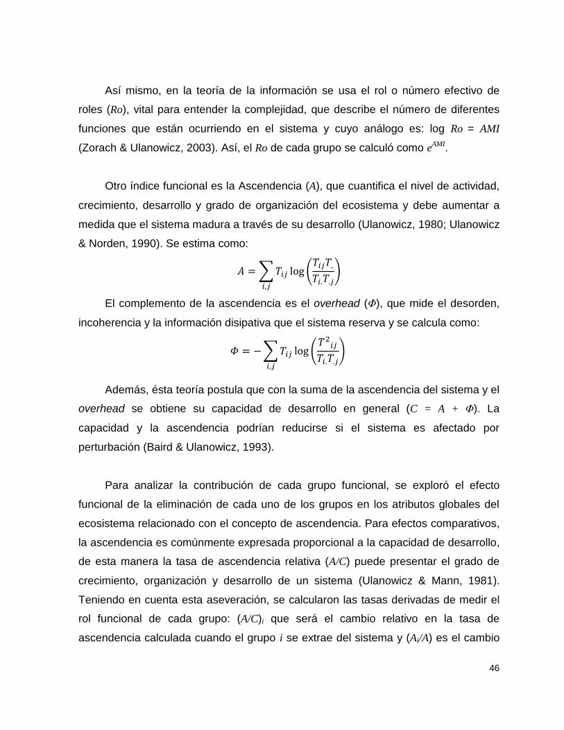
46
Así mismo, en la teoría de la información se usa el rol o número efectivo de
roles (Ro), vital para entender la complejidad, que describe el número de diferentes
funciones que están ocurriendo en el sistema y cuyo análogo es: log Ro = AMI
(Zorach & Ulanowicz, 2003). Así, el Ro de cada grupo se calculó como eAMI.
Otro índice funcional es la Ascendencia (A), que cuantifica el nivel de actividad,
crecimiento, desarrollo y grado de organización del ecosistema y debe aumentar a
medida que el sistema madura a través de su desarrollo (Ulanowicz, 1980; Ulanowicz
& Norden, 1990). Se estima como:
𝐴 = ∑ 𝑇𝑖𝑗
𝑖,𝑗
log (𝑇𝑖𝑗𝑇..
𝑇𝑖.𝑇.𝑗)
El complemento de la ascendencia es el overhead (Φ), que mide el desorden,
incoherencia y la información disipativa que el sistema reserva y se calcula como:
𝛷 = − ∑ 𝑇𝑖𝑗
𝑖,𝑗
log (𝑇2
𝑖𝑗
𝑇𝑖.𝑇.𝑗)
Además, ésta teoría postula que con la suma de la ascendencia del sistema y el
overhead se obtiene su capacidad de desarrollo en general (C = A + Φ). La
capacidad y la ascendencia podrían reducirse si el sistema es afectado por
perturbación (Baird & Ulanowicz, 1993).
Para analizar la contribución de cada grupo funcional, se exploró el efecto
funcional de la eliminación de cada uno de los grupos en los atributos globales del
ecosistema relacionado con el concepto de ascendencia. Para efectos comparativos,
la ascendencia es comúnmente expresada proporcional a la capacidad de desarrollo,
de esta manera la tasa de ascendencia relativa (A/C) puede presentar el grado de
crecimiento, organización y desarrollo de un sistema (Ulanowicz & Mann, 1981).
Teniendo en cuenta esta aseveración, se calcularon las tasas derivadas de medir el
rol funcional de cada grupo: (A/C)i que será el cambio relativo en la tasa de
ascendencia calculada cuando el grupo i se extrae del sistema y (Ai/A) es el cambio

47
relativo de la ascendencia cuando el grupo i es extrae del sistema, con respecto a la
ascendencia original (Riofrío-Lazo et al., 2013). En este mismo sentido, se calculó el
aporte de cada grupo funcional o especie de la ictiofauna al FADI y el indicador (O/C)
que representa la redundancia en el sistema (Arreguín-Sánchez, 2014). En el caso
del FADI, para las especies que no son peces, se usó el valor de la diversidad
funcional calculado para cada periodo en el capítulo 2. Para efectos de comparación
y evaluar el rol de los grupos de peces en el ecosistema, la ictiofauna fue analizada
en dos grupos teniendo en cuenta el nivel trófico (TL<3,0 y TL>3,0).
4.1.3. Resultados
Las matrices con los valores de los índices ecológicos y ecosistémicos
estimados para valorar la contribución de cada grupo al funcionamiento del
ecosistema se muestran en el Anexo 4.2. Para el análisis del papel de las especies
de la ictiofauna en el ecosistema se tuvo en cuenta las variables (A/C)i, D, Ro, TL,
O/C, B y P/B, por ser las que mostraron correlaciones significativas más fuertes
(rs>0,70) y el FADI para comparar el índice de diversidad funcional con los índices
ecológicos y ecosistémicos (Figura 4.1). Una fuerte correlación positiva fue
encontrada entre el índice (A/C)i con Ro y TL (Correlación de Sperman rs=0,96 y 0,79
respectivamente; p<0,05). En este mismo sentido, entre la variable D con B y con Ro
pero esta última fue negativa (rs=0,90 y -0,73 respectivamente; p<0,05). En el caso
de TL, se relacionó significativamente con otras variables como Ro (rs = 0,82), (O/C)i
(rs=-0,79) y (A/C)i (rs=0,79), entre otras variables. El índice de diversidad funcional
FADI, sólo se relacionó significativamente de manera débil con las variables (A/C)i y
(O/C)i (rs=-0,37 en ambos casos) (Figura 4.1). El indicador de cambio relativo de la
ascendencia (Ai/A) por cada grupo funcional se relacionó significativamente con
diversas variables pero más fuertemente con Ro (rs > 0,90), (A/C)i y (O/C)i.

Fig
ura
4.1
. M
atr
iz d
e c
orr
ela
cio
nes e
ntr
e a
lgu
nos d
e l
os in
dic
adore
s e
co
lóg
icos (
dato
s de e
ntr
ad
a a
l m
ode
lo,
va
lore
s e
stim
ados d
el
an
ális
is
ecosis
tém
ico
e índ
ice d
e d
ivers
idad f
uncio
na
l).
46

49
En el análisis de la tendencia de los índices, se observa que en el Ro
contrastado con el aporte relativo de cada grupo al orden del sistema (A/C), muestra
como los niveles tróficos menores a tres tienen un rol menor que las especies del
nivel trófico superior a tres, pero tienen un aporte relativo más alto al orden del
sistema para el primer periodo (Figura 4.2). Durante los otros dos periodos, la
tendencia observada fue totalmente contraria al periodo inicial, en donde las especies
con valores de rol más alto y con mayor aporte al orden del sistema fueron las
especies de niveles tróficos superiores, sobre todo en el periodo de 1998. Por otra
parte, para 2011 los grupos parecen acomodarse en la parte central del diagrama,
indicando que el aporte al orden y el rol en el sistema se presentan en las mismas
proporciones tanto los niveles tróficos superiores como los inferiores (Figura 4.2).
Caso similar sucede en la tendencia de la relación del índice de grado (D) y el rol
(Ro), donde las especies de nivel trófico superior tuvieron un rol mayor pero con
menor índice de grado en 1980. A diferencia de la anterior comparación, esta
tendencia se mantuvo durante los otros dos periodos, pero para 2011 las diferencias
entre especies de los niveles tróficos mayores y menores a tres no fueron tan
marcadas.
En la correlación entre el nivel trófico (TL) y el rol (Ro), se evidencia un cambio
en su tendencia, mostrando para los periodos inicial y final una pendiente positiva, es
decir, los niveles tróficos superiores presentan los mayores valores de rol que los
inferiores. En el periodo intermedio (1998), la pendiente a pesar de ser positiva tiende
a estar cercana a cero, por lo que todos los niveles tróficos tendrían el mismo rol en
el sistema. El índice (O/C) como medidor de redundancia, comparado con el índice
de diversidad funcional no evidencia una clara tendencia, pero fue posible observar
que el aporte relativo a la redundancia del sistema por la ictiofauna fue mayor en el
periodo inicial que en los otros dos periodos (Figura 4.4).

50
Figura 4.2. Diagrama de dispersión para visualizar la tendencia entre los índices seleccionados para
los grupos de peces en1980 (arriba), 1998 (medio) y 2011 (abajo): Ro contra (A/C)i y D. Los símbolos
en negro indican especies de peces de nivel trófico superior a tres y los rojos niveles tróficos inferiores
a tres. AGU: Agujas, ANC: Anchovetas, ANG: Anguilas, BAG: Bagres, BAR: Barbudos, CIN: Cintillas,
COR: Corvinas, IGU: Iguanas, ISA: Isabelitas, JUR: Jureles, LIS: Lisas, MER: Meros, MOJ: Mojarras,
MOM: Mojarras mexicanas, PAR: Pargos, GLO: Peces Globo, PLA: Peces Planos, ROC: Peces Roca,
PEJ: Pejesapos, PER: Pericos, RAY: Rayas, ROB: Robalos, RON: Roncos, SAR: Sardinas, SAG:
Sargos.

51
Figura 4.3. Diagrama de dispersión para la visualización de la tendencia entre los índices Ro y TL para
los periodos 1980 (izquierda), 1998 (centro) y 2011 (derecha).
Figura 4.4. Relación entre el índice de diversidad funcional FADI y el índice de redundancia relativa
(O/C) para 1980 (izquierda), 1998 (centro) y 2011 (derecha). Los símbolos en negro indican especies
de peces de nivel trófico superior a tres y los rojos niveles tróficos inferiores a tres. AGU: Agujas, ANC:
Anchovetas, ANG: Anguilas, BAG: Bagres, BAR: Barbudos, CIN: Cintillas, COR: Corvinas, IGU:
Iguanas, ISA: Isabelitas, JUR: Jureles, LIS: Lisas, MER: Meros, MOJ: Mojarras, MOM: Mojarras
mexicanas, PAR: Pargos, GLO: Peces Globo, PLA: Peces Planos, ROC: Peces Roca, PEJ:
Pejesapos, PER: Pericos, RAY: Rayas, ROB: Robalos, RON: Roncos, SAR: Sardinas, SAG: Sargos.

52
En cuanto a la relación del nivel trófico (TL) y el indicador de redundancia,
mostró que ligeramente los niveles trófico inferiores (TL<3,0) hacen mayor aporte a la
redundancia del sistema (Figura 4.5). Así mismo, en el análisis de rol (Ro) y el aporte
relativo de cada grupo a la ascendencia (Ai/A) se observó que durante el primer
periodo las especies de niveles tróficos menores a tres tenían un rol menos relevante
en cuanto al aporte en la ascendencia del ecosistema, y que con el paso del tiempo,
este rol se ha igualado con especies de niveles tróficos mayores (TL>3,0) (Figura
4.6).
Figura 4.5. Diagrama de dispersión para la visualización de la tendencia entre los índices TL y (O/C)i
para los periodos 1980 (izquierda), 1998 (centro) y 2011 (derecha).
Figura 4.6. Diagrama de dispersión para la visualización de la tendencia entre los índices Ro y (Ai/A)
para los periodos 1980 (izquierda), 1998 (centro) y 2011 (derecha).

53
4.1.4. Discusión
La valoración del crecimiento y desarrollo de los ecosistemas se ha basado
principalmente en la medición de los flujos de energía utilizados para describir su
estructura y funcionamiento (Scharler, 2009). Dentro de la estructura y
funcionamiento del ecosistema, cada componente posee un rol para el
mantenimiento del balance. El uso del índice de grado para expresar la importancia
de un grupo funcional dentro de la red trófica, usado muchas veces como índice de
especie clave (Sole & Montoya, 2001), por sí solo representa solamente la
importancia estructural. Al usarlo con otros indicadores ecológicos se podría conocer
la contribución ecológica al ecosistema. Los resultados sugieren que especies con el
mismo valor del índice de grado, presentan roles diferentes, siendo las especies de
más altos niveles tróficos los que juegan roles más relevantes en el ecosistema. Por
otro lado, estas especies con nivel trófico inferior (TL<3.0) realizaban un aporte
mayor al orden del sistema en 1980, no así para los dos periodos más recientes
donde especies de nivel trófico superior (TL>3.0), realizaron mayores aportes al
orden del sistema, contribuyendo a la especialización y madurez del ecosistema
(Riofrío-Lazo et al., 2013)
La importancia de una especie puede ser discutida en dos sentidos: (1) la que
representa para el ecosistema y la naturaleza y (2) la importancia para los científicos
y público en general (Riofrío-Lazo et al., 2013). En un ecosistema, la resiliencia está
relacionada con cambios en su estructura y función, lo que podría significar cambios
en diferentes atributos del ecosistema como la producción, diversidad, omnivoría, la
relación biomasa/respiración, entre otros (Arreguín-Sánchez, 2014). La relación entre
el potencial de crecimiento del sistema (O) y su capacidad de desarrollo (C), O/C,
representa a la redundancia en el sistema, que en el caso de la Laguna de Términos
durante los tres periodos de evaluación se observaron cambios siendo mayor en el
periodo inicial (1980) que los otros dos periodos. Incluso, este indicador fue menor
para el último periodo. En este mismo sentido, las especies de nivel trófico menor a

54
tres influyeron más en la relación O/C para el periodo inicial, mientras que en los
otros dos periodos, la tendencia es que todos los peces tienen el mismo aporte a la
redundancia del sistema. Dado esto, se esperaba que tuviese el mismo
comportamiento que el índice de diversidad funcional, para evaluar la posibilidad de
tener dos indicadores de funcionalidad por dos fuentes diferentes. Sin embargo, los
resultados no fueron consistentes aunque la correlación haya sido negativa y
significativa, y en el segundo periodo el aporte de los peces a la redundancia del
sistema haya disminuido en comparación con 1980.
Por otro lado, el aporte de las especies de las dos categorías de niveles tróficos
a la redundancia fue muy similar en los tres periodos, es decir que en término de
organización y resiliencia realizan los mismos aportes (Ulanowicz, 2002) a pesar de
mostrar una diversidad funcional diferente. Esto significa que diferentes funciones en
el sistema contribuirían casi de la misma manera a la organización del sistema. En un
ecosistema, los grupos funcionales con un rol similar ayudan a que la estructura,
organización y funcionamiento se mantengan con el paso del tiempo (Chapin III et al.,
2000). Con esto en mente y conociendo el aporte de cada grupo funcional a la
resiliencia del ecosistema, se observó que con el paso del tiempo esta ha disminuido
paulatinamente poniendo en peligro su estabilidad o balance. Esto significa una baja
en la reserva de energía del ecosistema que tendría para resistir embates lo que
podría verse reflejado en una disminución en la resistencia y menor capacidad de
recuperación para volver al estado inicial (Arreguín-Sánchez, 2014). Así mismo, esta
disminución en la reserva de energía puede ver disminuía la capacidad de mantener
la estructura y funcionalidad del ecosistema (Walker, 1992).
Por otro lado, el hecho de que las especies contribuyan más o menos de la
misma forma a la resiliencia y el hecho de que los valores de diversidad funcional de
los grupos funcionales cambien en la escala temporal podría evidenciar un
mecanismo de re-estructuración del sistema relacionado con su capacidad de auto-
organización. En este mismo sentido, la disminución de los niveles de organización y
resiliencia puede comprometer su potencial de auto-organización (Ulanowicz, 1980;

55
Costanza & Mageau, 1999). Es importante mencionar el grupo de peces ha sido
destacado como el de mayor aporte a la resiliencia del ecosistema (Ulanowicz, 1986;
Ruiz-Barreiro, 2012).
Los grupos funcionales mostraron comportamiento similares en cuanto al rol en
el ecosistema, este resultado es consistente con lo reportado por Arreguín-Sánchez
& Ruiz-Barreiro (2014) quienes, a través de simulaciones, estimaron la vulnerabilidad
relativa de distintos ecosistemas, señalando que para el caso de la Laguna de
Términos, la simulación mostró que perturbando ciertos grupos funcionales
relacionados a los peces (e.g. Mojarras, Roncos, Bagres), la medida de orden (A/C)
mostró poca variación y, por el contrario, cuando se perturbaron otros grupos (e.g.
camarones, fitoplancton, zooplanton, microcrutáceos) la ganancia o pérdida del orden
fue evidente.
Los cambios en los aportes de cada grupo funcional podrían estar dados por la
simple dinámica de la laguna, que encuentra una alternancia entre especies del
mismo grupo funcional o incluso con otras especies u otros grupos equivalentes
funcionalmente. Lo anterior, sumado a la reserva u overhead, lideran los procesos de
auto-organización para el mantenimiento del orden en el ecosistema. En este
contexto, la remoción de alguna de las especies o en su defecto de algunas de las
funciones alteraría la función y organización del ecosistema (Srivastava, 2002; Duffy,
2008; Arreguín-Sánchez & Ruiz-Barreiro, 2014).
Otro punto que hay que destacar es un cambio en el aporte al orden o a la
entropía (desorden) del ecosistema. Para el periodo inicial (1980), las especies de
niveles tróficos medios a altos hacen mayor aporte al orden, mientras que las de
niveles tróficos menores lo hacen a la entropía, y por tanto a la vulnerabilidad del
ecosistema (Arreguín-Sánchez & Ruiz-Barreiro, 2014). Contrario a lo acontecido para
el periodo inicial, los siguientes periodos el rol fue cambiado siendo los niveles
tróficos bajos (TL<3.0) los de mayor aporte al orden. Este intercambio en los roles de
cada uno de los grupos funcionales de la ictiofauna evidencian su importancia en los

56
procesos de resiliencia, capacidad, sostenibilidad y auto-organización, conceptos que
están fuertemente relacionados (Ulanowicz et al., 2009).
La respuesta dinámica del ecosistema, mostrada en los tres periodos evaluados
con cada uno de los indicadores usados, evidencia la no linealidad y complejidad de
un proceso como lo es la auto-organización, en donde cada uno de sus componentes
también obedece a las interacciones con otros miembros del ecosistema y con el
medio (Camazine et al., 2003). Los procesos de auto-organización están regidos por
algunos procesos ecológicos como son la sucesión, la estabilidad y la teoría del caos
(Margalef, 1968; Odum, 1983; Hansson & Helgesson, 2003). La ascendencia,
indicador del crecimiento de un ecosistema dentro de estos indicadores, también
representa la cantidad de enlaces que pueden implicar una capacidad de auto
organización que ayudará a una etapa de madurez y desarrollo (Ulanowicz, 1986).
Así, el mayor aporte relativo de cada grupo funcional al crecimiento del ecosistema
como soporte a estos procesos de auto-organización fue dado por los grupos de
peces con niveles tróficos menores a tres, y con el paso del tiempo se fueron
estabilizando en la medida de igualar sus aportes a ambos grupos de peces. Es
importante mencionar que el aporte fue mucho mayor en el primer periodo que
durante los dos periodos siguientes.
Por otro lado, un ecosistema puede mantener orden si tiene energía de reserva
suficiente, lo que generará un aumento en la entropía (Ulanowicz, 1986).
Relacionado con los procesos de auto-organización, a mayor relación del indicador
del orden del ecosistema (A/C) menor será la capacidad de auto-organización
(Ulanowicz et al., 2009). En este estudio, las especies de peces con niveles tróficos
menores a tres, mostraron bajos aportes a la auto-organización del ecosistema de la
laguna, durante el primer periodo (1980) en comparación con los otros dos periodos
(1998 y 2011). A nivel específico, los sargos (SAR) presentaron los mayores
cambios, siendo menor el aporte en 1980 que en los otros dos periodos. No sucedió
lo mismo con la ictiofauna de niveles trófico mayores a tres que mostraron la misma
tendencia en los tres periodos, a excepción del grupo de las corvinas (COR) que para

57
el primer periodo tenía lo mayores aportes en los procesos de auto-organización y
para los otros dos periodos fue inferior, incluso por debajo de especies del grupo de
niveles tróficos menores a tres.

5. DISCUSIÓN GENERAL

59
La Laguna de Términos es considerada un ecosistema estuarino crítico e
importante con una alta productividad (primaria y secundaria), diversidad ecológica y
de importancia para las distintas pesquerías que se realizan en el sur del Golfo de
México. Está conectada funcionalmente con la zona adyacente (Sonda de
Campeche) y dadas las condiciones hidrobiológicas, estacionalidad ambiental y
complejidades de orden social, económico y ecológico han hecho que su manejo sea
muy complicado (Yáñez-Arancibia & Day Jr, 2005).
El estudio desde la perspectiva ecológica se ha direccionado al uso de
indicadores que evalúan sus atributos ecológicos (riqueza, diversidad, índices
taxonómicos) y como estos responden a la variabilidad climática (Sosa-Lopez, 2005).
Solamente en los últimos años, se ha destacado el uso de la diversidad funcional
para evaluar la estructura funcional de este ecosistema, siempre teniendo presente
que para mantener la estructura y el funcionamiento del ecosistema es importante la
biodiversidad (para la robustez del ecosistema), modularidad (desarrollo de
subestructuras dentro de la red trófica) y redundancia funcional (variedad de
especies con el mismo rol funcional) (Arreguín-Sánchez, 2014; Abascal-Monroy et
al., 2015). Esta última (roles ecológicos similares) es de vital importancia para la
estabilidad del ecosistema y una disminución provocaría una pérdida de la
redundancia de especies en el ecosistema (Navia et al., 2016). En la Laguna se
denotó un aumento en la redundancia funcional del periodo de 1998, y mayor
equidad en los periodos 1980 y 2011. Lo anterior como consecuencia de una mayor
presencia de rasgos funcionales menos comunes, dada posiblemente por la
presencia de muchas especies marinas que visitan la laguna debido a su variabilidad
climática, influenciada por los diferenciales aportes de agua dulce de los principales
afluentes, las entradas de agua salina, la precipitación anual y fuertes vientos que
afectan las condiciones de los diferentes hábitats (Yáñez-Arancibia & Day Jr, 2005).
Esta presencia de especies marinas, que bien podrían ser consumidores de recursos
dentro de la laguna, influyen en la abundancia, distribución y estructura de la
población de las presas e indirectamente influyen en el funcionamiento del
ecosistema (Estes et al., 2001). Igualmente, la alta diversidad de hábitats estuarinos

60
y las diferentes fuentes de productividad primaria (principalmente manglares, pastos
marinos y vegetación arrastrada por los ríos que desembocan en la laguna) influyen
notablemente en la abundancia de la comunidad íctica y su diversidad, dada la alta
correlación entre el ambiente físico y los procesos biológicos del ecosistema lagunar
(Yáñez-Arancibia & Day, 1982; Sosa-Lopez, 2005; Yáñez-Arancibia & Day Jr, 2005).
Por otro lado, la variabilidad en el entorno pueden afectar algunas especies más
que a otras como resultado de sus diferentes características biológicas, ecológicas y
de historia de vida (Mouillot et al., 2012; Sirot et al., 2015). Aunque la profundidad fue
la variable abiótica de mayor influencia en la diversidad ecológica, se ha destacado
que la salinidad es importante en el control de la biodiversidad, la distribución de
organismos y la abundancia de los distintos grupos bióticos. Así mismo, la
transparencia afecta a la productividad de los productores primarios en la columna de
agua (fitoplancton, microalgas, macroalgas y pastos marinos) (Yáñez-Arancibia &
Day Jr, 2005). La primera de ellas fue mayor y la segunda menor durante 1998
respecto a los otros dos periodos estudiados. Además de estas variables, la
variabilidad del pH y la transparencia, afectan a la estructura comunitaria (Ramos-
Miranda et al., 2005a), e incluso a los atributos biológicos y funcionales (Sirot et al.,
2015).
Otro aspecto a destacar es que los cambios en la intensidad y dirección de las
interacciones ecológicas entre las aguas de la Laguna de Términos y la Sonda de
Campeche provocan cambios en la diversidad, distribución, abundancia y
persistencia de los recursos (Yáñez-Arancibia & Day Jr, 2005). Esto puede explicar el
hecho que la equivalencia funcional de las especies presente cambios a lo largo de
los tres periodos analizados alternando algunas especies entre los periodos pero
siempre teniendo especies dominantes dentro de cada uno de los bloques de la
equivalencia funcional. Esta respuesta también puede deberse al hecho que los
ecosistemas en general no tienen un equilibrio como tal, de modo que están
cambiando de composición, contenido o tratamiento de los nutrientes y la energía
(Pickett & Cadenasso, 2002). Incluso se ha destacado que aún no se logra entender

61
como las especies persisten en las redes tróficas complejas aun cuando sufran
perturbaciones rápidas y fuertes (Montoya et al., 2006).
Una característica importante de la cadena trófica de la laguna es su alta
conectividad (Yáñez-Arancibia & Day Jr, 2005; Abascal-Monroy et al., 2015), por lo
que podría reflejarse en que todos los grupos de peces realizan la misma
contribución a la organización del ecosistema. Por eso, además de poseer roles
ecológicos como la transformación de la energía a partir de los productores
primarios, transferencia activa de esta energía a través de la cadena trófica,
intercambio de energía entre los sistemas vecinos a través de la migración,
almacenamiento de energía en el ecosistema y actores en la regulación de la
energía, poseen roles importantes y semejantes en el orden y estructura del sistema.
Así mismo, aquellas que mayores aportes hacen a la diversidad ecológica tienen
menores aportes a la reserva del sistema. En el análisis de los ecosistemas a través
de la modelación de la biodiversidad, ha sido importante el incluir el papel de la
riqueza de especies, especies clave, grupos funcionales y el ensamblaje en los
procesos del ecosistema, ya que podrían aclarar el papel de cada uno de
componentes de la diversidad en la función de los ecosistemas (Pickett &
Cadenasso, 2002)
Por otra parte, se ha destacado que la resiliencia y la organización (A/C)
disminuye con el incremento de la temperatura (Christian et al., 2005; Arreguín-
Sánchez, 2014) pero nuestros resultados muestran que quizás la respuesta no sólo
está dada por el aumento de la temperatura sino por otros factores externos
forzantes. Por ejemplo, si se tiene en cuenta el índice multivariado del niño, se
observan tres momentos diferentes para los tres periodos evaluados (1980-1981 año
“normal”; 1998-1999 “niño fuerte”; 2010-2011 “niña fuerte”; Figura 5.1). En este
mismo sentido, cambios interdecadales en la estructura trófica han sido asociados
con modificaciones hidrológicas en ecosistemas estuarinos (Baird & Heymans, 1996;
Christian et al., 2005). Así mismo, se ha relacionado cambios interdecadales en las
interacciones tróficas influenciadas por la fluctuación climática decadal del Atlántico

62
Norte (AMO con oscilación entre 8 a 12 años) creando condiciones favorables y
desfavorables en la cuenca y que podrían influir en la dinámica de las poblaciones de
la laguna, como ha incidido en otros organismos en el Sur del Golfo de México (del
Monte-Luna et al., 2012; Arreguín-Sánchez et al., 2015)
Figura 5.1. Índice multivariado de oscilación del sur/”el niño” (ENSO por su sigla en inglés) para los
últimos 65 años. Se destacan dentro de los recuadros verdes los periodos de evaluación. Modificado
de: Observatorio_ARVAL (2016).
En este sentido, se destaca que la estructura comunitaria o grupos funcionales
de peces son de vital importancia para el mantenimiento de la estructura,
funcionamiento y productividad de consumidores de la Laguna de Términos (Yáñez-
Arancibia & Day Jr, 2005). Debido a que los ecosistemas marinos se encuentran en
constante cambio como respuesta a todas las perturbaciones, es importante destacar
el rol de las especies de peces con niveles tróficos menores a tres, quienes han
llevado el principal papel de soportar todas estas incidencias externas para mantener
la estructura, orden y funcionamiento del ecosistema en la Laguna de Términos
desde 1980, pero que ha ido en descenso con el paso del tiempo, llegando incluso a
igualarse con el otro grupo analizado (TL>3.0) con el paso del tiempo.
A nivel ecosistémico, es importante que esta reserva de energía que aún se
tiene la Laguna de Términos pueda mantenerse para recuperar el equilibrio. Llevar a
la laguna a sobrepasar los límites que impliquen un sistema en un estado alternativo,
podría comprometer su respuesta a perturbaciones naturales para el mantenimiento

63
de la estructura y funcionamiento. Así, para no llegar a esos límites es más fácil el
control sobre las afectaciones antrópicas como la deforestación y la sobrepesca para
mantener esta energía de reserva (Arreguín-Sánchez, 2014).

6. CONCLUSIONES GENERALES

65
La equidad funcional calculada a partir del FADI detectó una variabilidad
temporal influenciada por las variables ambientales, principalmente por la
profundidad y que podría estar relacionado con altas abundancias de
depredadores de altos niveles tróficos y afinidad marina como visitantes
ocasionales en la laguna asociado con cambios en la estructura funcional de las
comunidades biológicas de la laguna.
Los resultados obtenidos en el análisis de diversidad funcional entre los tres
periodos mostraron a dos periodos (1980 y 2011) dentro de la distribución de
probabilidad esperada, mientras que 1998 por fuera de esta distribución. La
evidencia generada apoya la idea de una reestructuración funcional de la
comunidad de peces. Aunque se ha demostrado cambios en la diversidad
taxonómica de peces de la laguna, también es importante evaluar aquellos
aspectos que estén relacionados con los rasgos funcionales para revelar
cambios en los procesos que contribuyen al su funcionamiento. Es así que los
resultados mostrados en la evaluación de la diversidad funcional, la laguna
evidencia una reorganización funcional durante los años estudiados.
Todos los peces juegan un papel importante en los flujos de nutrientes a lo
largo de los niveles tróficos. Es importante reconocer que existen especies que
pueden tener equivalentes funcionales en el elenco sistemático. Es por esto que
es de vital importancia aquellas especies recurrentes encontradas en el análisis
de equivalencia, que ha sido descritas como especies residentes, por lo cual se
deberían tener programas de conservación de estas para el mantenimiento de
la estructura y funcionamiento del ecosistema, ya que podrían ser los actores
claves en la reorganización de la estructura funcional.
Las especies de peces presentaron roles diferenciales teniendo en cuentas los
niveles tróficos superiores e inferiores a tres. Los primeros fueron más
importantes en mantener el orden en el ecosistema durante los dos periodos
más recientes, no así para el periodo de 1980, que los mayores aportes al
orden fueron realizados por la especies de niveles tróficos menores a tres.
La redundancia del sistema fue menor con el paso del tiempo. En el periodo
inicial fue mayor el aporte de la especies con niveles tróficos menores a tres a

66
la redundancia del sistema. En los otros dos periodos, todas las especies
realizaron el mismo aporte a la energía de reserva de la Laguna de Términos.
Dado que las dos categorías de niveles tróficos realizan aportes a la
organización y resiliencia del sistema, se demuestra que diferentes funciones
contribuyen de la misma manera a la organización del sistema.
Durante el análisis temporal, se observó una disminución de la reserva
energética (resiliencia) del sistema necesaria para su resistencia y recuperación
ante embates ambientales o antrópicos, por lo que se podría comprometer la
estructura y funcionamiento del ecosistema.
La alternancia entre los grupos de especies de peces en los roles que juegan
en el ecosistema evidencia los mecanismos de reestructuración del sistema
relacionado con su capacidad de auto-organización.
La respuesta dinámica del ecosistema, mostrada en los tres periodos evaluados
con cada uno de los indicadores usados, evidencia la no linealidad y
complejidad de un proceso como es la auto-organización, en donde cada uno
de sus componentes también obedece a las interacciones con otros miembros
del ecosistema y con el medio.
El mayor aporte relativo de las diferentes especies al crecimiento del
ecosistema, como soporte a estos procesos de auto-organización, fue dado por
los grupos de peces con niveles tróficos menores a tres en el primer periodo
evaluado. Para los periodos más recientes, los aportes de todas las especies
fueron muy similares.

67
REFERENCIAS
Abascal-Monroy, I.M. 2013. Comparación temporal del estado de la red trófica de la Laguna de Términos, Campeche, México durante 1980, 1998 y 2011. Tesis de Maestría, Centro Interdisciplinario de Ciencias Marinas. Instituto Politécnico Nacional. 108 p.
Abascal-Monroy, I.M., M.J. Zetina-Rejón, F. Escobar-Toledo, G.A. López-Ibarra, A. Sosa-López, & A. Tripp-Valdez. 2015. Functional and Structural Food Web Comparison of Terminos Lagoon, Mexico in Three Periods (1980, 1998, and 2011). Estuar. Coast., 1-12.
Álvarez-Filip, L., & H. Reyes-Bonilla. 2006. Comparison of community structure and functional diversity of fishes at Cabo Pulmo coral reef, Western Mexico between 1987 and 2003. Proc.10th Int. Coral Reef Symp, 216-225.
Allen, K.R. 1971. Relation between production and biomass. J. Fish. Res. Board Can., 28, 1573 - 1581.
Antony, P.J., S. Dhanya, P.S. Lyla, B.M. Kurup, & S. Ajmal Khan. 2010. Ecological role of stomatopods (mantis shrimps) and potential impacts of trawling in a marine ecosystem of the southeast coast of India. Ecol. Model., 221(21), 2604-2614.
Arreguín-Sánchez, F. 2014. Measuring resilience in aquatic trophic networks from supply–demand-of-energy relationships. Ecol. Model., 272, 271-276.
Arreguín-Sánchez, F., P. del Monte-Luna, & M.J. Zetina-Rejón. 2015. Climate Change Effects on Aquatic Ecosystems and the Challenge for Fishery Management: Pink Shrimp of the Southern Gulf of Mexico. Fisheries, 40(1), 15-19.
Arreguín-Sánchez, F., & T.M. Ruiz-Barreiro. 2014. Approaching a functional measure of vulnerability in marine ecosystems. Ecol. Indicators, 45, 130-138.
Baird, D., & J. Heymans. 1996. Assessment of ecosystem changes in response to freshwater inflow of the Kromme River estuary, St. Francis Bay, South Africa: a network analysis approach. Water SA, 22, 307-318.
Baird, D., & R.E. Ulanowicz. 1993. Comparative study on the trophic structure, cycling and ecosystem properties oi iour tidal. Mar. Ecol. Prog. Ser., 99, 221-237.

68
Balvanera, P., A.B. Pfisterer, N. Buchmann, J.S. He, T. Nakashizuka, D. Raffaelli, & B. Schmid. 2006. Quantifying the evidence for biodiversity effects on ecosystem functioning and services. Ecol. Lett., 9(10), 1146-1156.
Barberán, A., S.T. Bates, E.O. Casamayor, & N. Fierer. 2012. Using network analysis to explore co-occurrence patterns in soil microbial communities. The ISME journal, 6(2), 343-351.
Batagelj, V., P. Doreian, & A. Ferligoj. 1992. An optimizational approach to regular equivalence. Soc. Networks, 14(1), 121-135.
Blondel, J. 2003. Guilds or functional groups: does it matter? Oikos, 100, 223 - 231.
Borgatti, S.P., & M.G. Everett. 1989. The class of all regular equivalences: Algebraic structure and computation. Soc. Networks, 11(1), 65-88.
Borgatti, S.P., & M.G. Everett. 1993. Two algorithms for computing regular equivalence. Soc. Networks, 15(4), 361-376.
Borgatti, S.P., M.G. Everett, & L.C. Freeman. 2002. UCINET 6 for Windows: Software for Social Network Analysis (Version 6.232): Harvard: Analytic Technologies.
Borgatti, S.P., M.G. Everett, & J.C. Johnson. 2013. Analyzing social networks. SAGE Publications Limited. 290 p.
Bossel, H. 2000. Exergy and the Emergence of Multidimensional System Orientation, 193 - 209. En: Jørgensen, S.E. (Ed.), Thermodynamics and Ecological Modelling. Boca Ratón, FL. 384 p.
Botta-Dukát, Z. 2005. Rao's quadratic entropy as a measure of functional diversity based on multiple traits. J. Veg. Sci., 16(5), 533-540.
Boyd, J.P., & M.G. Everett. 1999. Relations, residuals, regular interiors, and relative regular equivalence. Soc. Networks, 21(2), 147-165.
Buisson, L., G. Grenouillet, S. Villéger, J. Canal, & L. Pascal. 2013. Toward a loss of functional diversity in stream fish assemblages under climate change. Glob Change Biol, 19, 387 - 400.
Camazine, S., J.-L. Deneubourg, N.R. Franks, J. Sneyd, G. Theraulaz, & E. Bonabeau. 2003. Self-organization in biological systems. Princeton University Press. 560 p.

69
Casanoves, F., L. Pla, J.A. Di Rienzo, & S. Díaz. 2011. FDiversity: a software package for the integrated analysis of functional diversity. Method Ecol Evol, 2(3), 233-237.
Clarke, K.R., & R.M. Warwick. 2001. Change in Marine Communities: An approach to Statisical Analysis and Interpretation. 2nd Edition. Primer-E Ltd. 169 p.
Cornwell, W.K., D.W. Schwilk, & D.D. Ackerly. 2006. A trait-based test for habitat filtering: convex hull volume. Ecology, 87(6), 1465-1471.
Costanza, R., & M. Mageau. 1999. What is a healthy ecosystem? Aquat. Ecol., 33(1), 105-115.
Cruz-Escalona, V.H., F. Arreguin-Sanchez, & M. Zetina-Rejon. 2007. Analysis of the ecosystem structure of Laguna Alvarado, western Gulf of Mexico, by means of a mass balance model. Estuar. Coast. Shelf Sci., 72(1), 155-167.
Cury, P., A. Bakun, R.J. Crawford, A. Jarre, R.A. Quiñones, L.J. Shannon, & H.M. Verheye. 2000. Small pelagics in upwelling systems: patterns of interaction and structural changes in “wasp-waist” ecosystems. ICES J. Mar. Sci., 57(3), 603-618.
Chapin III, F.S., E.S. Zavaleta, V.T. Eviner, R.L. Naylor, P.M. Vitousek, H.L. Reynolds, D.U. Hooper, S. Lavorel, O.E. Sala, & S.E. Hobbie. 2000. Consequences of changing biodiversity. Nature, 405(6783), 234-242.
Christensen, V., & D. Pauly. 1992. Ecopath II—a software for balancing steady-state ecosystem models and calculating network characteristics. Ecol. Model., 61(3), 169-185.
Christian, R.R., D. Baird, J. Luczkovich, J.C. Johnson, U.M. Scharler, & R.E. Ulanowicz. 2005. Role of network analysis in comparative ecosystem ecology of estuaries En: Belgrano, A., U.M. Scharler, J. Dunne & R.E. Ulanowicz (Eds.). Aquatic Food Webs: An Ecosystem Approach. Oxford University Press.Vol. 25-40. New York. 262 p.
Dale, V.H., & S.C. Beyeler. 2001. Challenges in the development and use of ecological indicators. Ecol. Indicators, 1(1), 3-10.
del Monte-Luna, P., V. Guzmán-Hernández, E.A. Cuevas, F. Arreguín-Sánchez, & D. Lluch-Belda. 2012. Effect of North Atlantic climate variability on hawksbill turtles in the Southern Gulf of Mexico. J. Exp. Mar. Biol. Ecol., 412, 103-109.

70
Duffy, J.E. 2008. Why biodiversity is important to the functioning of real-world ecosystems. Front. Ecol. Environ., 7(8), 437-444.
Dumay, O., P. Tari, J. Tomasini, & D. Mouillot. 2004. Functional groups of lagoon fish species in Languedoc Roussillon, southern France. J. Fish Biol., 64(4), 970-983.
Emirbayer, M., & J. Goodwin. 1994. Network analysis, culture, and the problem of agency. Am. J. Sociol., 1411-1454.
Estes, J., K. Crooks, & R. Holt. 2001. Ecological role of predators, 857 - 878. En: Levin, S.A. (Ed.), Encyclopedia of Biodiversity. Academic Press.Vol. 4. University of Minnesota. 917 p.
Everett, M.G., & S.P. Borgatti. 1994. Regular equivalence: General theory. J. Math. Sociol., 19(1), 29-52.
Fan, T.F., C.J. Liau, & T.Y. Lin. (2007). Positional analysis in fuzzy social networks. En: Young-Lin, T., X. Hu, J. Han, X. Shen & Z. Li (Eds.). Proceedings IEEE International Conference on Granular Computing, 2007, Silicon Valley, California. 423-428.
Flynn, D.F., M. Gogol‐Prokurat, T. Nogeire, N. Molinari, B.T. Richers, B.B. Lin, N. Simpson, M.M. Mayfield, & F. DeClerck. 2009. Loss of functional diversity under land use intensification across multiple taxa. Ecol. Lett., 12(1), 22-33.
Galeana-Cortazar, A.R. 2015. Fuentes orgánicas de carbono y su relación con la ictiofauna dominante en Laguna de Términos, Campeche, México. Tesis de Maestría, Instituto Politécnico Nacional. Centro Interdisciplinario de Ciencias Marinas. 83 p.
Garrison, L.P., & J.S. Link. 2000. Fishing effects on spatial distribution and trophic guild structure of the fish community in the Georges Bank region. ICES J. Mar. Sci., 57(3), 723-730.
Goldstein, R.M., & M.R. Meador. 2005. Multilevel assessment of fish species traits to evaluate habitat degradation in streams of the upper Midwest. N. Am. J. Fish. Manage., 25(1), 180-194.
Gristina, M., T. Bahri, F. Fiorentino, & G. Garofalo. 2006. Comparison of demersal fish assemblages in three areas of the Strait of Sicily under different trawling pressure. Fish. Res., 81(1), 60-71.
Hansson, S.O., & G. Helgesson. 2003. What is stability? Synthese, 136(2), 219-235.

71
Herrera-Silveira, J.A., A. Silva, P. Salles, G. Villalobos-Zapata, I. Medina, J. Espinal, A. Zaldivar, J. Trejo, M. González, A. Cu, & J. Ramirez. 2002. Análisis de la calidad ambiental usando indicadores hidrobiológicos y modelo hidrodinámico actualizado de Laguna de Términos. CINVESTAV-IPN, Mérida, EPOMEX-Instituto de Ingeniería-UNAM. 187 p.
Heymans, J., R. Ulanowicz, & C. Bondavalli. 2002. Network analysis of the South Florida Everglades graminoid marshes and comparison with nearby cypress ecosystems. Ecol. Model., 149(1), 5-23.
Heymans, J.J., S. Guénette, & V. Christensen. 2007. Evaluating network analysis indicators of ecosystem status in the Gulf of Alaska. Ecosystems, 10(3), 488-502.
Hooper, D.U., M. Solan, A. Symstad, S. Diaz, M.O. Gessner, N. Buchmann, V. Degrange, P. Grime, F. Hulot, & F. Mermillod-Blondin. 2002. Species diversity, functional diversity and ecosystem functioning, 195-208. En: Loreau, M., S. Naeem & P. Inchausti (Eds.). Biodiversity and Ecosystem Functioning: Synthesis and Perspectives. Oxford University Press. 299 p.
Huse, G. 2012. Ecosystem Ecology: a New Synthesis. Mar. Biol. Res., 8(5-6), 568-569.
Jordán, F., W.c. Liu, & A.J. Davis. 2006. Topological keystone species: measures of positional importance in food webs. Oikos, 112(3), 535-546.
Jordán, F., T.A. Okey, B. Bauer, & S. Libralato. 2008. Identifying important species: linking structure and function in ecological networks. Ecol. Model., 216(1), 75-80.
Krebs, C.J. 2003. Ecología. Estudio de la distribución y abundancia. Oxford University Press México. 753 p.
Lankford, R.R. 1977. Coastal lagoons of Mexico, their origin and classification, 182 - 215. En: Wiley, M. (Ed.), Estuarine Processes II: Circulation, Sediments, and Transfer of material in the estuary. Academic Press Inc. New York. 428 p.
Libralato, S., V. Christensen, & D. Pauly. 2006. A method for identifying keystone species in food web models. Ecol. Model., 195(3), 153-171.
Lombarte, A., A. Gordoa, A.K. Whitfield, N.C. James, & V.M. Tuset. 2012. Ecomorphological analysis as a complementary tool to detect changes in fish communities following major perturbations in two South African estuarine systems. Environ. Biol. Fishes, 94(4), 601-614.

72
Luczkovich, J.J., S.P. Borgatti, J.C. Johnson, & M.G. Everett. 2003. Defining and measuring trophic role similarity in food webs using regular equivalence. J. Theor. Biol., 220(3), 303-321.
Mageau, M.T., R. Costanza, & R.E. Ulanowicz. 1998. Quantifying the trends expected in developing ecosystems. Ecol. Model., 112(1), 1-22.
Magurran, A.E. 1988. Ecological diversity and its measurement. Princeton University Press New Jersey. 179 p.
Manickchand-Heileman, S., F. Arreguín-Sánchez, A. Lara-Domínguez, & L. Soto. 1998. Energy flow and network analysis of Terminos Lagoon, SW Gulf of Mexico. J. Fish Biol., 53, 179-197.
Margalef, R. 1968. Perspectives in ecological theory. Univ. Chicago Press Chicago. 111 p.
Mason, N.W., K. MacGillivray, J.B. Steel, & J.B. Wilson. 2003. An index of functional diversity. J. Veg. Sci., 14(4), 571-578.
Mason, N.W., D. Mouillot, W.G. Lee, & J.B. Wilson. 2005. Functional richness, functional evenness and functional divergence: the primary components of functional diversity. Oikos, 111(1), 112-118.
Medina, M., M. Araya, & C. Vega. 2004. Alimentación y relaciones tróficas de peces costeros de la zona norte de Chile. Invest. Mar., 32(1), 33-47.
Mizruchi, M.S. 1993. Cohesion, equivalence, and similarity of behavior: a theoretical and empirical assessment. Soc. Networks, 15(3), 275-307.
Molina, J.L., Á. Quiroga, J. Martí Olivé, I. Maya Jariego, & A.d. Federico. 2006. Talleres de autoformación con programas informáticos de análisis de redes sociales. Universitat Autònoma de Barcelona. 107 p.
Montoya, J.M., S.L. Pimm, & R.V. Solé. 2006. Ecological networks and their fragility. Nature, 442(7100), 259-264.
Mouillot, D., N.A. Graham, S. Villéger, N.W. Mason, & D.R. Bellwood. 2012. A functional approach reveals community responses to disturbances. Trends Ecol. Evol.

73
Mouillot, D., S. Villéger, M. Scherer-Lorenzen, & N.W. Mason. 2011. Functional structure of biological communities predicts ecosystem multifunctionality. PloS one, 6(3), e17476.
Naeem, S., & S. Li. 1997. Biodiversity enhances ecosystem reliability. Nature, 390, 507-509.
Naeem, S., & J.P. Wright. 2003. Disentangling biodiversity effects on ecosystem functioning: deriving solutions to a seemingly insurmountable problem. Ecol. Lett., 6(6), 567-579.
Navia, A.F., E. Cortés, & P.A. Mejía-Falla. 2010. Topological analysis of the ecological importance of elasmobranch fishes: A food web study on the Gulf of Tortugas, Colombia. Ecol. Model., 221(24), 2918-2926.
Navia, A.F., V.H. Cruz-Escalona, A. Giraldo, & A. Barausse. 2016. The structure of a marine tropical food web, and its implications for ecosystem-based fisheries management. Ecol. Model., 328, 23-33.
Observatorio_ARVAL. 2016. Cambio Climático ("Calentamiento Global"?). Revisado en: Marzo de 2016, En: http://www.oarval.org/CambioClimaBW.htm.
Odum, E.P. 1983. Basic ecology. Saunders College Publishing New York. 446 p.
Odum, E.P., G.W. Barrett, & M.T.A. Ortega. 2006. Fundamentos de Ecología. Thomson México. 598 p.
Pahl-Wostl, C., & R.E. Ulanowicz. 1993. Quantification of species as functional units within an ecological network. Ecol. Model., 66(1-2), 65-79.
Palacios-Salgado, D.S. 2011. Patrones latitudinales de composición y diversidad funcional de peces asociados a la pesca de camarón del Pacífico mexicano Tesis de M. Sc., Instituto Politécnico Nacional, México. 129 p.
Pascual, M., & J.A. Dunne. 2006. Ecological networks: linking structure to dynamics in food webs. Oxford University Press, USA New York. 386 p.
Pauly, D. 1989. Food consumption by tropical and temperate marine fishes: some generalizations. J. Fish Biol., 35(Supplement A), 11 - 20.
Pauly, D., V. Christensen, & C. Walters. 2000. Ecopath, Ecosim, and Ecospace as tools for evaluating ecosystem impact of fisheries. ICES J. Mar. Sci., 57(3), 697-706.

74
Petchey, O.L., K.L. Evans, I.S. Fishburn, & K.J. Gaston. 2007. Low functional diversity and no redundancy in British avian assemblages. J. Anim. Ecol., 76(5), 977-985.
Pickett, S.T., & M.L. Cadenasso. 2002. The ecosystem as a multidimensional concept: meaning, model, and metaphor. Ecosystems, 5(1), 1-10.
Ramos-Miranda, J. 2000. Biologie, ecologie, exploitation de la crevette blanche Litopenaeus setiferus en Campeche, mexique. Tesis de Doctorado Especialidad: Oceanografía, L’université de Bretagne Occidentale. 320 p.
Ramos-Miranda, J., D. Flores-Hernandez, A. Sosa-Lopez, L. Ayala-Perez, S. Villéger, M. Pérez-Sánchez, F. Gómez-Criollo, M. Can-González, E. Flores-Ramos, & D. Mouillot. 2015. La comunidad del necton en la laguna de Términos: modificación del hábitat vs cambios en la comunidad, 181 - 197. En: Ramos-Miranda, J. & G. Villalobos-Zapata (Eds.). Aspectos socioambientales de la región de la laguna de Términos, Campeche. Universidad Autónoma de Campeche. Campeche. 210 p.
Ramos-Miranda, J., D. Mouillot, D. Flores-Hernandez, A. Sosa-Lopez, T. Do-Chi, & L. Ayála-Pérez. 2005a. Changes in four complementary facets of fish diversity in a tropical coastal lagoon after 18 years: a functional interpretation. Mar. Ecol. Prog. Ser., 304, 1-13.
Ramos-Miranda, J., L. Quiniou, D. Flores-Hernandez, T. Do-Chi, L. Ayala-Perez, & A. Sosa-Lopez. 2005b. Spatial and temporal changes in the nekton of the Terminos Lagoon, Campeche, Mexico. J. Fish Biol., 66(2), 513-530.
Riofrío-Lazo, M., F. Arreguín-Sánchez, M. Zetina-Rejón, & F. Escobar-Toledo. 2013. The Ecological Role of the Vaquita, Phocoena sinus, in the Ecosystem of the Northern Gulf of California. Ecosystems, 16, 416-433.
Ruiz-Barreiro, T.M. 2012. Procesos dinámicos subyacentes al concepto de salud del ecosistema. Tesis de Maestría, Instituto Politécnico Nacional. 96 p.
Scharler, U.M. 2009. Ecological Network Analysis, Ascendency, 57-64. En: Jørgensen, S.E. (Ed.), Ecosystems Ecology. Elsevier B.V. Amsterdam. 521 p.
Scharler, U.M., & D. Baird. 2005. A comparison of selected ecosystem attributes of three South African estuaries with different freshwater inflow regimes, using network analysis. J. Mar. Syst., 56(3), 283-308.
Schleuter, D., M. Daufresne, F. Massol, & C. Argillier. 2010. A user's guide to functional diversity indices. Ecol. Monogr., 80(3), 469-484.

75
Sirot, C., S. Villéger, D. Mouillot, A. Darnaude, J. Ramos-Miranda, D. Flores-Hernandez, & J. Panfili. 2015. Combinations of biological attributes predict temporal dynamics of fish species in response to environmental changes. Ecol. Indicators, 48, 147-156.
Solé, R.V., & J. Bascompte. 2006. Self-Organization in Complex Ecosystems. Princeton University Press New Jersey. 373 p.
Sole, R.V., & M. Montoya. 2001. Complexity and fragility in ecological networks. Proc. R. Soc. B, 268(1480), 2039-2045.
Somerfield, P.J., K.R. Clarke, R.M. Warwick, & N.K. Dulvy. 2008. Average functional distinctness as a measure of the composition of assemblages. ICES J. Mar. Sci., 65(8), 1462-1468.
Sosa-Lopez, A. 2005. Ecological processes and dynamics of the fish communities in the Terminos Lagoon, Gulf of Mexico. Tesis de Ph.D. Thesis, L’Université Montpellier, France. 162 p.
Sosa-López, A., D. Mouillot, T. Do Chi, & J. Ramos-Miranda. 2005. Ecological indicators based on fish biomass distribution along trophic levels: an application to the Terminos coastal lagoon, Mexico. ICES J. Mar. Sci., 62(3), 453-458.
Srivastava, D.S. 2002. The role of conservation in expanding biodiversity research. Oikos, 98(2), 351-360.
Tilman, D. 2001. Functional diversity, 109-120. En: Levin, S. (Ed.), Encyclopedia of biodiversity. Academic Press.Vol. 3. San Diego. 871 p.
Tilman, D., J. Knops, D. Wedin, P. Reich, M. Ritchie, & E. Siemann. 1997. The influence of functional diversity and composition on ecosystem processes. Science, 277(5330), 1300-1302.
Tobor-Kapłon, M.A., R. Holtkamp, U.M. Scharler, A. Doroszuk, F.J. Kuenen, J. Bloem, & P.C. De Ruiter. 2007. Evaluation of information indices as indicators of environmental stress in terrestrial soils. Ecol. Model., 208(1), 80-90.
Ulanowicz, R.E. 1980. An hypothesis on the development of natural communities. J. Theor. Biol., 85(2), 223-245.
Ulanowicz, R.E. 1986. Growth and development: ecosystems phenomenology. Springer-Verlag New York. 203 p.

76
Ulanowicz, R.E. 1997. Ecology, the ascendent perspective. Columbia University Press. 201 p.
Ulanowicz, R.E. 2001. Information theory in ecology. Comput. Chem., 25(4), 393-399.
Ulanowicz, R.E. 2002. Toward quantifying semiotic agencies: Habits Arising. J. Semiotics Evol. Energy. Dev., 2(1), 38-55.
Ulanowicz, R.E. 2004. Quantitative methods for ecological network analysis. Comput. Biol. Chem., 28(5), 321-339.
Ulanowicz, R.E., S.J. Goerner, B. Lietaer, & R. Gomez. 2009. Quantifying sustainability: Resilience, efficiency and the return of information theory. Ecol. Complex., 6(1), 27-36.
Ulanowicz, R.E., & K.H. Mann. 1981. Ecosystems under stress, 133 - 137. En: Platt, T., K.H. Mann & R.E. Ulanowicz (Eds.). Mathematical Models in Biological Oceanography. UNESCO Press. Paris. 156 p.
Ulanowicz, R.E., & J.S. Norden. 1990. Symmetrical overhead in flow networks. Int. J. Syst. Sci., 21(2), 429-437.
Vasconcellos, M., S. Mackinson, K. Sloman, & D. Pauly. 1997. The stability of trophic mass-balance models of marine ecosystems: a comparative analysis. Ecol. Model., 100(1-3), 125-134.
Villalobos-Zapata, G., G. Palacio-Aponte, A. Sosa-López, H. Alvaez-Guillén, & A. Reda-Deara. 2002. Ecología del paisaje y Diagnóstico Ambiental del ANP “Laguna de Términos”. Informe Final. SISIERRA P/SISIERRA 20000706030. 199 p.
Villéger, S., N.W. Mason, & D. Mouillot. 2008. New multidimensional functional diversity indices for a multifaceted framework in functional ecology. Ecology, 89(8), 2290-2301.
Villéger, S., P.M. Novack‐Gottshall, & D. Mouillot. 2011. The multidimensionality of the niche reveals functional diversity changes in benthic marine biotas across geological time. Ecol. Lett., 14(6), 561-568.
Villéger, S., J. Ramos-Miranda, D. Flores-Hernandez, & D. Mouillot. 2012. Low functional β-diversity despite high taxonomic β-diversity among tropical estuarine fish communities. PloS one, 7(7), e40679.

77
Villéger, S., J. Ramos-Miranda, D. Flores-Hernández, & D. Mouillot. 2010. Contrasting changes in taxonomic vs. functional diversity of tropical fish communities after habitat degradation. Ecol. Appl., 20(6), 1512-1522.
Wainwright, P.C., D.R. Bellwood, & M.W. Westneat. 2002. Ecomorphology of locomotion in labrid fishes. Environ. Biol. Fishes, 65(1), 47-62.
Walker, B.H. 1992. Biodiversity and ecological redundancy. Conserv. Biol., 6(1), 18-23.
Wright, J.P., S. Naeem, A. Hector, C. Lehman, P.B. Reich, B. Schmid, & D. Tilman. 2006. Conventional functional classification schemes underestimate the relationship with ecosystem functioning. Ecol. Lett., 9(2), 111-120.
Yáñez-Arancibia, A., & J. Day Jr. 2005. Managing Freshwater Inflows to Estuaries. Ecosystem Functioning: The basis for sustainable management of Términos Lagoon, Campeche, Mexico. Instituto de Ecología. Jalapa, Veracruz. 76 p.
Yañez-Arancibia, A., & J.W. Day. 2005. Ecosystem Functioning: The basis for sustainable management of Términos Lagoon, Campeche, México. Jalapa, México: Institute or Ecology. 77 p.
Yáñez-Arancibia, A., & J.W. Day. 1982. Ecological characterization of Terminos Lagoon, a tropical lagoon-estuarine system in the southern Gulf of Mexico. Oceanol. Acta, 5(4), 462-472.
Yáñez-Arancibia, A., A.L. Lara-Domínguez, P. Sánchez-Gil, H. Alvarez-Guillen, I. Vargas-Maldonado, A. Aguirre-León, M. Tapia-Garcia, M. Garcia-Abad, D. Flores-Hernandez, P. Chavance, F. Amezcua-Linares, S. Diaz-Ruiz, M. Alvarez-Rubio, & J.L. Rojas-Galaviz. 1982. Caracterización ambiental del sistema ecológico y análisis comparativo de las poblaciones de peces de la Sonda de Campeche y de la Laguna de Términos, antes y después del derrame petrolero del Pozo IXTOC-I. Final Report. PCEESC/UNAM/ICML/ (IF). 221 p.
Zetina-Rejón, M.J. 2004. Efectos de la pesca en ecosistemas inter-dependientes: Laguna de Términos y Sonda de Campeche, México. Tesis de Ph. D., Instituto Politécnico Nacional, México. 106 p.
Zetina-Rejón, M.J., F. Arreguın-Sánchez, & E.A. Chavez. 2003. Trophic structure and flows of energy in the Huizache–Caimanero lagoon complex on the Pacific coast of Mexico. Estuar. Coast. Shelf Sci., 57(5), 803-815.

78
Zorach, A.C., & R.E. Ulanowicz. 2003. Quantifying the complexity of flow networks: how many roles are there? Complexity, 8(3), 68-76.

ANEXOS

A
nexo
3.1
. Mat
riz d
e in
cid
enci
a q
ue
repr
esen
ta la
re
laci
ón e
ntre
las
espe
cie
s y
sus
rasg
os
fun
cion
ale
s. O
GO
=O
vípa
ros
Ges
taci
ón O
ral,
OH
BF
P=
Oví
paro
s h
uevo
s be
ntón
icos
y f
ase
pel
ágic
a, O
HB
SF
P=
Oví
paro
s h
uevo
s b
entó
nico
s y
sin
fase
pel
ágic
a, O
HP
=O
vípa
ros
huev
os
pelá
gico
s, O
VO
=O
vovi
vípa
ros,
DF
B=
De
mer
sal F
ondo
s B
land
os, D
FD
=D
eme
rsal
Fo
ndos
Dur
os,
DF
M=
Dem
ersa
l Fon
dos
Mix
tos
Es
pec
ie -
198
0
2 - 2.50
2.51 - 3.00
3.01 - 3.50
3.51 - 4.00
> 4.00
OGO
OHBFP
OHBSFP
OHP
OVO
Ictioinvertivoros
Piscivoros
Invertívoros
Omnívoros
Planctívoros
Anguiliforme
Compresiforme
Depresiforme A
Depresiforme B
Fusiforme
Globiforme
Sagitiforme
Teniforme
Otras Formas
Oblicua
Superior
Terminal
Aca
ntho
stra
cion
qua
dric
orni
s 0
01
00
00
01
00
01
0
00
00
00
10
00
00
1A
chiru
s lin
eatu
s 0
00
10
00
01
00
01
0
00
01
00
00
00
01
0A
lute
rus
scho
epfii
1
00
00
00
01
00
00
0
10
10
00
00
00
00
1A
ncho
a he
pset
us
00
10
00
00
10
00
1
0 0
01
00
00
00
00
00
Anc
hoa
lam
prot
aeni
a 0
01
00
00
01
00
01
0
00
10
00
00
00
00
0A
ncho
a m
itchi
lli 0
01
00
00
01
00
01
0
00
10
00
00
00
00
0A
ncyl
opse
tta o
mm
ata
00
01
00
00
10
00
1
0 0
00
10
00
00
00
01
Arc
hosa
rgus
pr
obat
ocep
halu
s 0
01
00
00
01
00
01
0
00
10
00
00
00
00
0A
rcho
sarg
us rh
ombo
idal
is
00
10
00
00
10
00
1
0 0
01
00
00
00
00
00
Ario
psis
felis
0
01
00
10
00
01
00
0
00
00
10
00
00
00
0B
agre
mar
inus
0
01
00
10
00
01
00
0
00
00
10
00
00
00
0B
aird
iella
chr
ysou
ra
00
01
00
00
10
00
1
0 0
01
00
00
00
00
00
Bai
rdie
lla ro
nchu
s 0
00
10
00
01
00
01
0
00
10
00
00
00
00
0B
othu
s oc
ella
tus
00
01
00
00
10
10
0
0 0
00
10
00
00
00
01
Car
anx
hipp
os
00
01
00
00
10
10
0
0 0
01
00
00
00
00
00
Cat
horo
ps m
elan
opus
0
00
10
10
00
00
00
1
00
00
10
00
00
00
0C
entro
pom
us u
ndec
imal
is
00
00
10
10
00
10
0
0 0
01
00
00
00
00
00
Cet
engr
aulis
ede
ntul
us
10
00
00
00
10
00
0
0 1
01
00
00
00
00
00
Cha
etod
ipte
rus
fabe
r 0
01
00
00
01
00
00
1
00
10
00
00
00
00
1C
hilo
myc
teru
s sc
hoep
fii
00
10
00
00
10
00
1
0 0
00
00
01
00
00
01
Chl
oros
com
brus
chr
ysur
us
00
01
00
00
10
10
0
0 0
01
00
00
00
00
00
Chr
iodo
rus
athe
rinoi
des
01
00
00
10
00
00
0
0 1
00
00
00
10
00
00
Cic
hlas
oma
urop
htha
lmum
0
00
10
10
00
01
00
0
00
10
00
00
00
00
0C
ithar
icht
hys
spilo
pter
us
00
01
00
00
10
00
0
1 0
00
10
00
00
00
01
Cyn
osci
on a
rena
rius
00
00
10
00
10
00
1
0 0
01
00
00
00
00
00
Cyn
osci
on n
ebul
osus
0
00
10
00
01
00
01
0
00
10
00
00
00
00
0C
ynos
cion
not
hus
00
00
10
00
10
00
1
0 0
01
00
00
00
00
00
80

C
ontin
uaci
ón A
nexo
3.1
.
Es
pec
ie -
198
0
2 - 2.50
2.51 - 3.00
3.01 - 3.50
3.51 - 4.00
> 4.00
OGO
OHBFP
OHBSFP
OHP
OVO
Ictioinvertivoros
Piscivoros
Invertívoros
Omnívoros
Planctívoros
Anguiliforme
Compresiforme
Depresiforme A
Depresiforme B
Fusiforme
Globiforme
Sagitiforme
Teniforme
Otras Formas
Oblicua
Superior
Terminal
Das
yatis
has
tata
0
01
00
00
00
10
01
0 0
00
10
00
00
00
00
Das
yatis
sab
ina
0 0
10
00
00
01
00
10
00
01
00
00
00
00
0D
iapt
erus
rhom
beus
0
01
00
00
01
00
01
0 0
01
00
00
00
00
00
Etro
pus
cros
sotu
s 0
01
00
00
01
00
01
0 0
00
10
00
00
00
01
Euc
inos
tom
us a
rgen
teus
0
01
00
00
01
00
01
0 0
01
00
00
00
00
00
Euc
inos
tom
us g
ula
0 0
10
00
00
10
00
10
00
10
00
00
00
00
0E
ucin
osto
mus
m
elan
opte
rus
0 0
10
00
00
10
00
10
00
10
00
00
00
00
0E
uger
res
plum
ieri
0 0
10
00
00
10
00
10
00
10
00
00
00
00
0G
obio
nellu
s oc
eani
cus
0 0
10
00
01
00
00
01
00
00
01
00
00
00
0H
aem
ulon
bon
arie
nse
0 0
01
00
00
10
00
10
00
10
00
00
00
00
0H
aem
ulon
plu
mie
rii
0 0
01
00
00
10
00
10
00
10
00
00
00
00
0H
aren
gula
jagu
ana
0 0
10
00
00
10
00
10
00
10
00
00
00
00
1H
ippo
cam
pus
erec
tus
0 0
10
00
00
01
00
10
00
00
00
00
01
00
0La
goce
phal
us la
evig
atus
0
00
01
00
01
01
00
0 0
00
00
01
00
00
01
Lutja
nus
anal
is
0 0
01
00
00
10
10
00
00
10
00
00
00
00
0Lu
tjanu
s gr
iseu
s 0
00
01
00
01
01
00
0 0
01
00
00
00
00
00
Lutja
nus
syna
gris
0
00
10
00
01
01
00
0 0
01
00
00
00
00
00
Men
ticirr
hus
amer
ican
us
0 0
10
00
00
10
00
10
00
10
00
00
00
00
0M
entic
irrhu
s sa
xatil
is
0 0
01
00
00
10
00
10
00
10
00
00
00
00
0M
icro
pogo
nias
un
dula
tus
0 0
10
00
00
10
00
10
00
10
00
00
00
00
0N
icho
lsin
a us
ta u
sta
1 0
00
00
00
10
00
00
10
10
00
00
00
00
1O
dont
osci
on d
ente
x 0
01
00
00
01
00
01
0 0
01
00
00
00
00
00
Olig
oplit
es s
auru
s 0
00
10
00
01
01
00
0 0
01
00
00
00
00
00
Oph
icht
hus
gom
esii
0 0
01
00
00
10
10
00
01
00
00
00
00
00
1O
pist
hone
ma
oglin
um
0 0
10
00
00
10
00
10
00
10
00
00
00
00
1O
psan
us b
eta
0 0
01
00
01
00
00
10
00
00
10
00
00
01
0O
rthop
ristis
chr
ysop
tera
0
00
10
00
01
00
01
0 0
01
00
00
00
00
00
Pol
ydac
tylu
s oc
tone
mus
0
00
10
00
01
00
00
1 0
01
00
00
00
00
00
81

C
ontin
uaci
ón A
nexo
3.1
.
Es
pec
ie -
198
0
2 - 2.50
2.51 - 3.00
3.01 - 3.50
3.51 - 4.00
> 4.00
OGO
OHBFP
OHBSFP
OHP
OVO
Ictioinvertivoros
Piscivoros
Invertívoros
Omnívoros
Planctívoros
Anguiliforme
Compresiforme
Depresiforme A
Depresiforme B
Fusiforme
Globiforme
Sagitiforme
Teniforme
Otras Formas
Oblicua
Superior
Terminal
Por
icht
hys
poro
siss
imus
0
00
10
00
10
01
00
0
00
00
10
00
00
01
0P
riono
tus
bean
ii 0
01
00
00
01
01
00
0
00
00
10
00
00
00
0P
riono
tus
caro
linus
0
00
01
00
01
01
00
0
00
00
10
00
00
00
0P
riono
tus
punc
tatu
s 0
00
10
00
01
01
00
0
00
00
10
00
00
00
0P
riono
tus
scitu
lus
00
00
10
00
10
10
0 0
0
00
01
00
00
00
00
Prio
notu
s tri
bulu
s 0
00
10
00
01
01
00
0
00
00
10
00
00
00
0S
corp
aena
plu
mie
ri 0
00
10
00
01
01
00
0
00
10
00
00
00
00
0S
elen
e vo
mer
0
00
10
00
01
01
00
0
00
10
00
00
00
00
0S
phoe
roid
es g
reel
eyi
00
10
00
00
10
00
1 0
0
00
00
01
00
00
01
Sph
oero
ides
nep
helu
s 1
00
00
00
01
00
01
0
00
00
00
10
00
00
1S
phoe
roid
es s
peng
leri
00
10
00
00
10
00
1 0
0
00
00
01
00
00
01
Sph
oero
ides
test
udin
eus
00
10
00
00
10
00
1 0
0
00
00
01
00
00
01
Ste
llife
r lan
ceol
atus
0
00
10
00
01
00
01
0
00
10
00
00
00
00
0S
teph
anol
epis
his
pidu
s 0
10
00
00
01
00
01
0
00
10
00
00
00
00
1S
ymph
urus
pla
gius
a 0
10
00
00
01
00
01
0
00
01
00
00
00
00
1S
yngn
athu
s lo
uisi
anae
0
01
00
00
00
10
01
0
01
00
00
00
00
00
0S
yngn
athu
s sc
ovel
li 0
01
00
00
00
10
01
0
01
00
00
00
00
00
0S
ynod
us fo
eten
s 0
00
01
00
01
00
10
0
00
00
00
01
00
10
0Tr
ichi
urus
lept
urus
0
00
01
00
01
01
00
0
00
00
00
00
10
00
0Tr
inec
tes
mac
ulat
us
01
00
00
00
10
00
1 0
0
00
10
00
00
00
01
Uro
batis
jam
aice
nsis
0
00
10
00
00
11
00
0
00
01
00
00
00
00
0 82

C
ont
inu
ació
n A
nexo
3.1
.
Es
pec
ie -
198
0
Inferior
Ventral
Protáctil
Tubular
Incluida
Proyectante
Semiventral
Redondeada
Truncada
Emarginada
Semilunada
Bifurcada
Confluente
Punteada
Forma de S
Doble emarginada
Sin caudal
Asimétrica Elasmo
0 - 300
301 - 600
> 600
Pelágico
Demersopelagico
DFB
DFD
DFM
Bentonico
Aca
ntho
stra
cion
qua
dric
orni
s 0
00
00
00
10
00
00
00
00
00
10
00
00
10
Ach
irus
linea
tus
00
00
00
01
00
00
0 0
00
00
10
00
00
00
1A
lute
rus
scho
epfii
0
00
00
00
10
00
00
00
00
00
10
01
00
00
Anc
hoa
heps
etus
0
01
00
00
00
00
10
00
00
01
00
10
00
00
Anc
hoa
lam
prot
aeni
a 0
01
00
00
00
00
10
00
00
01
00
10
00
00
Anc
hoa
mitc
hilli
00
10
00
00
00
01
0 0
00
00
10
01
00
00
0A
ncyl
opse
tta o
mm
ata
00
00
00
00
00
00
0 1
00
00
10
00
00
00
1A
rcho
sarg
us p
roba
toce
phal
us
10
00
00
00
00
01
0 0
00
00
01
00
00
01
0A
rcho
sarg
us rh
ombo
idal
is
10
00
00
00
00
01
0 0
00
00
01
00
00
01
0A
riops
is fe
lis
10
00
00
00
00
01
0 0
00
00
00
10
01
00
0B
agre
mar
inus
1
00
00
00
00
00
10
00
00
00
01
00
10
00
Bai
rdie
lla c
hrys
oura
0
00
00
10
00
00
00
00
10
01
00
00
10
00
Bai
rdie
lla ro
nchu
s 0
00
00
10
00
00
00
00
10
00
10
00
10
00
Bot
hus
ocel
latu
s 0
00
00
00
10
00
00
00
00
01
00
00
00
01
Car
anx
hipp
os
00
00
01
00
00
01
0 0
00
00
00
10
10
00
0C
atho
rops
mel
anop
us
10
00
00
00
00
01
0 0
00
00
10
00
10
00
0C
entro
pom
us u
ndec
imal
is
00
00
01
00
00
01
0 0
00
00
00
10
00
01
0C
eten
grau
lis e
dent
ulus
0
01
00
00
00
00
10
00
00
01
00
10
00
00
Cha
etod
ipte
rus
fabe
r 0
00
00
00
00
10
00
00
00
00
01
00
00
10
Chi
lom
ycte
rus
scho
epfii
0
00
00
00
10
00
00
00
00
01
00
01
00
00
Chl
oros
com
brus
chr
ysur
us
00
00
01
00
00
01
0 0
00
00
00
11
00
00
0C
hrio
doru
s at
herin
oide
s 1
00
00
00
00
00
10
00
00
01
00
10
00
00
Cic
hlas
oma
urop
htha
lmum
0
00
00
10
01
00
00
00
00
00
10
01
00
00
Cith
aric
hthy
s sp
ilopt
erus
0
00
00
00
00
00
00
10
00
01
00
00
00
01
Cyn
osci
on a
rena
rius
00
00
01
00
00
00
0 0
01
00
00
10
01
00
0C
ynos
cion
neb
ulos
us
00
00
01
00
01
00
0 0
00
00
00
10
01
00
0C
ynos
cion
not
hus
00
00
01
00
00
00
0 0
10
00
01
00
01
00
0D
asya
tis h
asta
ta
01
00
00
00
00
00
0 0
00
10
00
10
00
00
1
83

C
ont
inu
ació
n A
nexo
3.1
.
Es
pec
ie -
198
0
Inferior
Ventral
Protáctil
Tubular
Incluida
Proyectante
Semiventral
Redondeada
Truncada
Emarginada
Semilunada
Bifurcada
Confluente
Punteada
Forma de S
Doble emarginada
Sin caudal
Asimétrica Elasmo
0 - 300
301 - 600
> 600
Pelágico
Demersopelagico
DFB
DFD
DFM
Bentonico
Das
yatis
sab
ina
01
00
00
00
00
00
0 0
00
10
00
10
00
00
1 D
iapt
erus
rhom
beus
0
01
00
00
00
00
10
00
00
00
10
00
10
00
Etro
pus
cros
sotu
s 0
00
00
00
00
00
00
10
00
01
00
00
00
01
Euc
inos
tom
us a
rgen
teus
0
01
00
00
00
00
10
00
00
01
00
00
10
00
Euc
inos
tom
us g
ula
00
10
00
00
00
01
0 0
00
00
10
00
01
00
0 E
ucin
osto
mus
mel
anop
teru
s 0
01
00
00
00
00
10
00
00
01
00
00
10
00
Eug
erre
s pl
umie
ri 0
01
00
00
00
00
10
00
00
00
10
00
10
00
Gob
ione
llus
ocea
nicu
s 0
00
01
00
10
00
00
00
00
01
00
00
00
01
Hae
mul
on b
onar
iens
e 0
00
00
10
00
00
10
00
00
00
10
00
00
10
Hae
mul
on p
lum
ierii
0
00
00
10
00
00
10
00
00
00
10
00
00
10
Har
engu
la ja
guan
a 0
00
00
00
00
00
10
00
00
01
00
10
00
00
Hip
poca
mpu
s er
ectu
s 0
00
10
00
00
00
00
00
01
01
00
00
00
10
Lago
ceph
alus
laev
igat
us
00
00
00
00
00
10
0 0
00
00
00
11
00
00
0 Lu
tjanu
s an
alis
0
00
00
10
00
01
00
00
00
00
01
00
00
10
Lutja
nus
gris
eus
00
00
01
00
00
10
0 0
00
00
00
10
00
01
0 Lu
tjanu
s sy
nagr
is
00
00
01
00
00
10
0 0
00
00
00
10
00
01
0 M
entic
irrhu
s am
eric
anus
0
00
00
01
00
00
00
01
00
00
10
00
10
00
Men
ticirr
hus
saxa
tilis
0
00
00
01
00
00
00
01
00
00
10
00
10
00
Mic
ropo
goni
as u
ndul
atus
0
00
00
01
00
00
00
10
00
00
10
00
10
00
Nic
hols
ina
usta
ust
a 0
00
00
00
10
00
00
00
00
01
00
00
10
00
Odo
ntos
cion
den
tex
00
00
01
00
10
00
0 0
00
00
10
00
00
01
0 O
ligop
lites
sau
rus
00
00
01
00
00
01
0 0
00
00
01
00
10
00
0 O
phic
hthu
s go
mes
ii 0
00
00
00
00
00
01
00
00
00
01
00
00
10
Opi
stho
nem
a og
linum
0
00
00
00
00
00
10
00
00
00
10
10
00
00
Ops
anus
bet
a 0
00
00
00
10
00
00
00
00
01
00
00
00
10
Orth
opris
tis c
hrys
opte
ra
00
00
01
00
00
01
0 0
00
00
01
00
00
01
0 P
olyd
acty
lus
octo
nem
us
10
00
00
00
00
01
0 0
00
00
01
00
01
00
0 P
oric
hthy
s po
rosi
ssim
us
00
00
00
01
00
00
0 0
00
00
01
00
01
00
0
84

C
ontin
uaci
ón A
nexo
3.1
.
Es
pec
ie -
198
0
Inferior
Ventral
Protáctil
Tubular
Incluida
Proyectante
Semiventral
Redondeada
Truncada
Emarginada
Semilunada
Bifurcada
Confluente
Punteada
Forma de S
Doble emarginada
Sin caudal
Asimétrica Elasmo
0 - 300
301 - 600
> 600
Pelágico
Demersopelagico
DFB
DFD
DFM
Bentonico
Prio
notu
s be
anii
10
00
00
00
10
00
0 0
00
00
10
00
00
01
0 P
riono
tus
caro
linus
1
00
00
00
01
00
0 0
00
00
00
10
00
00
10
Prio
notu
s pu
ncta
tus
10
00
00
00
10
00
0 0
00
00
01
00
00
01
0 P
riono
tus
scitu
lus
10
00
00
00
10
00
0 0
00
00
10
00
00
01
0 P
riono
tus
tribu
lus
10
00
00
00
10
00
0 0
00
00
01
00
00
01
0 S
corp
aena
plu
mie
ri 0
00
00
10
01
00
0 0
00
00
00
10
00
00
10
Sel
ene
vom
er
00
00
01
00
00
01
0 0
00
00
01
00
10
00
0 S
phoe
roid
es g
reel
eyi
00
00
00
00
10
00
0 0
00
00
10
00
10
00
0 S
phoe
roid
es n
ephe
lus
00
00
00
01
00
00
0 0
00
00
10
00
10
00
0 S
phoe
roid
es s
peng
leri
00
00
00
01
00
00
0 0
00
00
10
00
10
00
0 S
phoe
roid
es te
stud
ineu
s 0
00
00
00
10
00
0 0
00
00
00
10
01
00
00
Ste
llife
r lan
ceol
atus
0
00
00
10
00
00
0 0
10
00
01
00
00
10
00
Ste
phan
olep
is h
ispi
dus
00
00
00
01
00
00
0 0
00
00
10
00
01
00
0 S
ymph
urus
pla
gius
a 0
00
00
00
00
00
0 1
00
00
01
00
00
00
01
Syn
gnat
hus
loui
sian
ae
00
01
00
01
00
00
0 0
00
00
01
00
01
00
0 S
yngn
athu
s sc
ovel
li 0
00
10
00
10
00
0 0
00
00
01
00
00
10
00
Syn
odus
foet
ens
00
00
00
00
00
01
0 0
00
00
01
00
00
01
0 Tr
ichi
urus
lept
urus
0
00
00
10
00
00
0 0
00
01
00
01
01
00
00
Trin
ecte
s m
acul
atus
0
00
00
00
10
00
0 0
00
00
01
00
00
00
01
Uro
batis
jam
aice
nsis
0
10
00
00
00
00
0 0
00
00
10
01
00
00
01
85

C
ont
inu
ació
n A
nexo
3.1
.
Es
pec
ie -
198
0
Marino
Mar-Anfídromo
Anádromo
Catádromo
Dulce
Dulce-Andrídromo
Oceanódromo
Aca
ntho
stra
cion
qua
dric
orni
s 1
00
00
00
Ach
irus
linea
tus
01
00
00
0A
lute
rus
scho
epfii
1
00
00
00
Anc
hoa
heps
etus
0
10
00
00
Anc
hoa
lam
prot
aeni
a 1
00
00
00
Anc
hoa
mitc
hilli
01
00
00
0A
ncyl
opse
tta o
mm
ata
10
00
00
0A
rcho
sarg
us p
roba
toce
phal
us
01
00
00
0A
rcho
sarg
us rh
ombo
idal
is
01
00
00
0A
riops
is fe
lis
01
00
00
0B
agre
mar
inus
0
10
00
00
Bai
rdie
lla c
hrys
oura
0
10
00
00
Bai
rdie
lla ro
nchu
s 0
10
00
00
Bot
hus
ocel
latu
s 1
00
00
00
Car
anx
hipp
os
00
00
00
1C
atho
rops
mel
anop
us
00
00
10
0C
entro
pom
us u
ndec
imal
is
01
00
00
0C
eten
grau
lis e
dent
ulus
0
10
00
00
Cha
etod
ipte
rus
fabe
r 0
00
00
01
Chi
lom
ycte
rus
scho
epfii
1
00
00
00
Chl
oros
com
brus
chr
ysur
us
01
00
00
0C
hrio
doru
s at
herin
oide
s 0
10
00
00
Cic
hlas
oma
urop
htha
lmum
0
00
00
10
Cith
aric
hthy
s sp
ilopt
erus
0
10
00
00
Cyn
osci
on a
rena
rius
01
00
00
0C
ynos
cion
neb
ulos
us
01
00
00
0C
ynos
cion
not
hus
01
00
00
0
86

C
ontin
uaci
ón A
nexo
3.1
.
Es
pec
ie -
198
0
Marino
Mar-Anfídromo
Anádromo
Catádromo
Dulce
Dulce-Andrídromo
Oceanódromo
Das
yatis
has
tata
0
10
00
00
Das
yatis
sab
ina
01
00
00
0D
iapt
erus
rhom
beus
0
10
00
00
Etro
pus
cros
sotu
s 0
00
00
01
Euc
inos
tom
us a
rgen
teus
0
10
00
00
Euc
inos
tom
us g
ula
01
00
00
0E
ucin
osto
mus
mel
anop
teru
s 0
10
00
00
Eug
erre
s pl
umie
ri 0
10
00
00
Gob
ione
llus
ocea
nicu
s 0
10
00
00
Hae
mul
on b
onar
iens
e 1
00
00
00
Hae
mul
on p
lum
ierii
1
00
00
00
Har
engu
la ja
guan
a 0
10
00
00
Hip
poca
mpu
s er
ectu
s 1
00
00
00
Lago
ceph
alus
laev
igat
us
01
00
00
0Lu
tjanu
s an
alis
0
10
00
00
Lutja
nus
gris
eus
01
00
00
0Lu
tjanu
s sy
nagr
is
10
00
00
0M
entic
irrhu
s am
eric
anus
0
00
00
01
Men
ticirr
hus
saxa
tilis
0
10
00
00
Mic
ropo
goni
as u
ndul
atus
0
10
00
00
Nic
hols
ina
usta
ust
a 1
00
00
00
Odo
ntos
cion
den
tex
10
00
00
0O
ligop
lites
sau
rus
01
00
00
0O
phic
hthu
s go
mes
ii 1
00
00
00
Opi
stho
nem
a og
linum
1
00
00
00
Ops
anus
bet
a 0
10
00
00
Orth
opris
tis c
hrys
opte
ra
00
00
00
1P
olyd
acty
lus
octo
nem
us
10
00
00
0
87

C
ontin
uaci
ón A
nexo
3.1
.
Es
pec
ie -
198
0
Marino
Mar-Anfídromo
Anádromo
Catádromo
Dulce
Dulce-Andrídromo
Oceanódromo
Por
icht
hys
poro
siss
imus
1
00
00
00
Prio
notu
s be
anii
10
00
00
0P
riono
tus
caro
linus
0
10
00
00
Prio
notu
s pu
ncta
tus
10
00
00
0P
riono
tus
scitu
lus
10
00
00
0P
riono
tus
tribu
lus
10
00
00
0S
corp
aena
plu
mie
ri 1
00
00
00
Sel
ene
vom
er
01
00
00
0S
phoe
roid
es g
reel
eyi
01
00
00
0S
phoe
roid
es n
ephe
lus
01
00
00
0S
phoe
roid
es s
peng
leri
01
00
00
0S
phoe
roid
es te
stud
ineu
s 0
10
00
00
Ste
llife
r lan
ceol
atus
0
10
00
00
Ste
phan
olep
is h
ispi
dus
10
00
00
0S
ymph
urus
pla
gius
a 0
10
00
00
Syn
gnat
hus
loui
sian
ae
10
00
00
0S
yngn
athu
s sc
ovel
li 0
10
00
00
Syn
odus
foet
ens
01
00
00
0Tr
ichi
urus
lept
urus
0
10
00
00
Trin
ecte
s m
acul
atus
0
10
00
00
Uro
batis
jam
aice
nsis
1
00
00
00
88

C
ont
inu
ació
n A
nexo
3.1
.
Es
pec
ie –
199
8
2 - 2.50
2.51 - 3.00
3.01 - 3.50
3.51 - 4.00
> 4.00
OGO
OHBFP
OHBSFP
OHP
OVO
Ictioinvertivoros
Piscivoros
Invertívoros
Omnívoros
Planctívoros
Anguiliforme
Compresiforme
Depresiforme A
Depresiforme B
Fusiforme
Globiforme
Sagitiforme
Teniforme
Otras Formas
Oblicua
Superior
Terminal
Aca
ntho
stra
cion
qua
dric
orni
s 0
01
00
00
01
00
0
1
00
00
00
01
00
00
0
1
Ach
irus
linea
tus
00
01
00
00
10
00
1
0
00
01
00
00
00
01
0
A
ncho
a he
pset
us
00
10
00
00
10
00
1
0
00
10
00
00
00
00
0
A
ncho
a m
itchi
lli 0
01
00
00
01
00
0
1
00
01
00
00
00
00
0
0
Arc
hosa
rgus
pro
bato
ceph
alus
0
01
00
00
01
00
0
1
00
01
00
00
00
00
0
0
Arc
hosa
rgus
rhom
boid
alis
0
01
00
00
01
00
0
1
00
01
00
00
00
00
0
0
Ario
psis
felis
0
01
00
10
00
01
0
0
00
00
01
00
00
00
0
0
Bag
re m
arin
us
00
10
01
00
00
10
0
0
00
00
10
00
00
00
0
B
aird
iella
chr
ysou
ra
00
01
00
00
10
00
1
0
00
10
00
00
00
00
0
B
aird
iella
ronc
hus
00
01
00
00
10
00
1
0
00
10
00
00
00
00
0
B
athy
gobi
us s
opor
ator
0
00
10
00
10
00
0
0
10
00
00
10
00
00
0
0
Bre
voor
tia g
unte
ri 1
00
00
00
01
00
0
0
01
01
00
00
00
00
0
1
Cal
amus
pen
na
00
10
00
00
10
00
1
0
00
10
00
00
00
00
0
C
aran
x cr
ysos
0
00
10
00
01
01
0
0
00
01
00
00
00
00
0
0
Car
anx
hipo
s 0
00
10
00
01
01
0
0
00
01
00
00
00
00
0
0
Cat
horo
ps m
elan
opus
0
00
10
10
00
00
0
0
10
00
01
00
00
00
0
0
Cen
tropo
mus
par
alle
lus
00
00
10
10
00
10
0
0
00
10
00
00
00
00
0
C
entro
pom
us p
oeyi
0
00
10
01
00
01
0
0
00
01
00
00
00
00
0
0
Cet
engr
aulis
ede
ntul
us
10
00
00
00
10
00
0
0
10
10
00
00
00
00
0
C
haet
odip
teru
s fa
ber
00
10
00
00
10
00
0
1
00
10
00
00
00
00
1
C
hilo
myc
teru
s sc
hoep
fii
00
10
00
00
10
00
1
0
00
00
00
10
00
00
1
C
hlor
osco
mbr
us c
hrys
urus
0
00
10
00
01
01
0
0
00
01
00
00
00
00
0
0
Cic
hlas
oma
urop
htha
lmum
0
00
10
10
00
01
0
0
00
01
00
00
00
00
0
0
Cith
aric
hthy
s sp
ilopt
erus
0
00
10
00
01
00
0
0
10
00
10
00
00
00
0
1
Con
odon
nob
ilis
00
10
00
00
10
00
1
0
00
10
00
00
00
00
0
C
ynos
cion
are
nariu
s 0
00
01
00
01
00
0
1
00
01
00
00
00
00
0
0
Cyn
osci
on n
ebul
osus
0
00
10
00
01
00
0
1
00
01
00
00
00
00
0
0
Das
yatis
sab
ina
00
10
00
00
01
00
1
0
00
01
00
00
00
00
0
D
iapt
erus
aur
atus
0
01
00
00
01
00
0
1
00
01
00
00
00
00
0
0
89

C
ontin
uaci
ón A
nexo
3.1
.
Es
pec
ie –
199
8
2 - 2.50
2.51 - 3.00
3.01 - 3.50
3.51 - 4.00
> 4.00
OGO
OHBFP
OHBSFP
OHP
OVO
Ictioinvertivoros
Piscivoros
Invertívoros
Omnívoros
Planctívoros
Anguiliforme
Compresiforme
Depresiforme A
Depresiforme B
Fusiforme
Globiforme
Sagitiforme
Teniforme
Otras Formas
Oblicua
Superior
Terminal
Dia
pter
us rh
ombe
us
00
10
00
00
10
00
1 0
0
01
00
00
00
00
00
Dor
osom
a pe
tene
nse
01
00
00
00
10
00
0 1
0
01
00
00
00
00
01
Elo
ps s
auru
s 0
00
10
00
01
01
00
0
00
00
00
01
00
00
1E
pine
phel
us it
ajar
a 0
00
01
00
01
01
00
0
00
10
00
00
00
00
0E
tropu
s cr
osso
tus
00
10
00
00
10
00
1 0
0
00
10
00
00
00
01
Euc
inos
tom
us a
rgen
teus
0
01
00
00
01
00
01
0
00
10
00
00
00
00
0E
ucin
osto
mus
gul
a 0
01
00
00
01
00
01
0
00
10
00
00
00
00
0E
ucin
osto
mus
mel
anop
teru
s 0
01
00
00
01
00
01
0
00
10
00
00
00
00
0E
uger
res
plum
ieri
00
10
00
00
10
00
1 0
0
01
00
00
00
00
00
Gob
ione
llus
ocea
nicu
s 0
01
00
00
10
00
00
1
00
00
01
00
00
00
0G
ymno
thor
ax s
axic
ola
00
01
00
00
10
10
0 0
0
10
00
00
00
00
01
Hae
mul
on a
urol
inea
tum
0
01
00
00
01
00
01
0
00
10
00
00
00
00
0H
aem
ulon
bon
arie
nse
00
01
00
00
10
00
1 0
0
01
00
00
00
00
00
Hae
mul
on p
lum
ierii
0
00
10
00
01
00
01
0
00
10
00
00
00
00
0H
aren
gula
jagu
ana
00
10
00
00
10
00
1 0
0
01
00
00
00
00
01
Hem
icar
anx
ambl
yrhy
nchu
s 0
01
00
00
01
01
00
0
00
10
00
00
00
00
0H
iman
tura
sch
mar
dae
00
01
00
00
01
00
1 0
0
00
10
00
00
00
00
Hip
poca
mpu
s er
ectu
s 0
01
00
00
00
10
01
0
00
00
00
00
01
00
0La
goce
phal
us la
evig
atus
0
00
01
00
01
01
00
0
00
00
00
10
00
00
1La
godo
n rh
ombo
ides
0
00
10
00
01
00
01
0
00
10
00
00
00
00
0Lo
bote
s su
rinam
ensi
s 0
00
01
00
01
01
00
0
00
10
00
00
00
00
0Lu
tjanu
s an
alis
0
00
10
00
01
01
00
0
00
10
00
00
00
00
0Lu
tjanu
s ap
odus
0
00
01
00
01
01
00
0
00
10
00
00
00
00
0Lu
tjanu
s gr
iseu
s 0
00
01
00
01
01
00
0
00
10
00
00
00
00
0Lu
tjanu
s sy
nagr
is
00
01
00
00
10
10
0 0
0
01
00
00
00
00
00
Men
ticirr
hus
amer
ican
us
00
10
00
00
10
00
1 0
0
01
00
00
00
00
00
Men
ticirr
hus
saxa
tilis
0
00
10
00
01
00
01
0
00
10
00
00
00
00
0M
icro
pogo
nias
und
ulat
us
00
10
00
00
10
00
1 0
0
01
00
00
00
00
00
Mon
acan
thus
cili
atus
0
10
00
00
01
00
00
1
00
10
00
00
00
00
1
90

C
ontin
uaci
ón A
nexo
3.1
.
Es
pec
ie –
199
8
2 - 2.50
2.51 - 3.00
3.01 - 3.50
3.51 - 4.00
> 4.00
OGO
OHBFP
OHBSFP
OHP
OVO
Ictioinvertivoros
Piscivoros
Invertívoros
Omnívoros
Planctívoros
Anguiliforme
Compresiforme
Depresiforme A
Depresiforme B
Fusiforme
Globiforme
Sagitiforme
Teniforme
Otras Formas
Oblicua
Superior
Terminal
Mug
il ce
phal
us
10
00
00
00
10
00
0 1
00
00
01
00
00
00
1M
ugil
cure
ma
10
00
00
00
10
00
0 1
00
00
01
00
00
00
1M
ycte
rope
rca
bona
ci
00
00
10
00
10
10
0 0
00
10
00
00
00
00
0N
icho
lsin
a us
ta u
sta
10
00
00
00
10
00
0 0
10
10
00
00
00
00
1O
cyur
us c
hrys
urus
0
00
10
00
01
00
01
0 0
01
00
00
00
00
00
Olig
oplit
es s
auru
s 0
00
10
00
01
01
00
0 0
01
00
00
00
00
00
Oph
icht
hus
gom
esii
00
01
00
00
10
10
0 0
01
00
00
00
00
00
1O
pist
hone
ma
oglin
um
00
10
00
00
10
00
1 0
00
10
00
00
00
00
1O
psan
us b
eta
00
01
00
01
00
00
1 0
00
00
10
00
00
01
0O
rthop
ristis
chr
ysop
tera
0
00
10
00
01
00
01
0 0
01
00
00
00
00
00
Pep
rilus
par
u 0
00
10
00
01
01
00
0 0
01
00
00
00
00
01
Pol
ydac
tylu
s oc
tone
mus
0
00
10
00
01
00
00
1 0
01
00
00
00
00
00
Por
icht
hys
poro
siss
imus
0
00
10
00
10
01
00
0 0
00
01
00
00
00
10
Prio
notu
s ca
rolin
us
00
00
10
00
10
10
0 0
00
00
10
00
00
00
0P
riono
tus
scitu
lus
00
00
10
00
10
10
0 0
00
00
10
00
00
00
0S
ardi
nella
bra
silie
nsis
0
01
00
00
01
00
01
0 0
01
00
00
00
00
01
Sel
ene
seta
pinn
is
00
01
00
00
10
10
0 0
00
10
00
00
00
00
0S
elen
e vo
mer
0
00
10
00
01
01
00
0 0
01
00
00
00
00
00
Sph
oero
ides
gre
eley
i 0
01
00
00
01
00
01
0 0
00
00
01
00
00
01
Sph
oero
ides
nep
helu
s 1
00
00
00
01
00
01
0 0
00
00
01
00
00
01
Sph
oero
ides
spe
ngle
ri 0
01
00
00
01
00
01
0 0
00
00
01
00
00
01
Sph
oero
ides
test
udin
eus
00
10
00
00
10
00
1 0
00
00
00
10
00
00
1S
telli
fer l
ance
olat
us
00
01
00
00
10
00
1 0
00
10
00
00
00
00
0S
teph
anol
epis
his
pidu
s 0
10
00
00
01
00
01
0 0
01
00
00
00
00
01
Stro
ngyl
ura
nota
ta n
otat
a 0
00
01
01
00
01
00
0 0
00
00
00
10
00
00
Sym
phur
us c
ivita
tium
0
01
00
00
01
00
01
0 0
00
10
00
00
00
01
Sym
phur
us p
lagi
usa
01
00
00
00
10
00
1 0
00
01
00
00
00
00
1S
yngn
athu
s lo
uisi
anae
0
01
00
00
00
10
01
0 0
10
00
00
00
00
00
Syn
gnat
hus
scov
elli
00
10
00
00
01
00
1 0
01
00
00
00
00
00
0
91

C
ontin
uaci
ón A
nexo
3.1
.
Es
pec
ie –
199
8
2 - 2.50
2.51 - 3.00
3.01 - 3.50
3.51 - 4.00
> 4.00
OGO
OHBFP
OHBSFP
OHP
OVO
Ictioinvertivoros
Piscivoros
Invertívoros
Omnívoros
Planctívoros
Anguiliforme
Compresiforme
Depresiforme A
Depresiforme B
Fusiforme
Globiforme
Sagitiforme
Teniforme
Otras Formas
Oblicua
Superior
Terminal
Syn
odus
foet
ens
0 0
00
10
00
10
01
0
0 0
00
00
00
10
01
00
Trac
hino
tus
caro
linus
0
00
10
00
01
00
01
0
00
10
00
00
00
00
0Tr
achi
notu
s fa
lcat
us
0 0
10
00
00
10
00
1
0 0
01
00
00
00
00
00
Trac
hino
tus
good
ei
0 0
00
10
00
10
00
1
0 0
01
00
00
00
00
00
Tric
hiur
us le
ptur
us
0 0
00
10
00
10
10
0
0 0
00
00
00
01
00
00
Trin
ecte
s m
acul
atus
0
10
00
00
01
00
01
0
00
01
00
00
00
00
1U
roba
tis ja
mai
cens
is
0 0
01
00
00
01
10
0
0 0
00
10
00
00
00
00
92

C
ont
inu
ació
n A
nexo
3.1
.
Es
pec
ie -
199
8
Inferior
Ventral
Protáctil
Tubular
Incluida
Proyectante
Semiventral
Redondeada
Truncada
Emarginada
Semilunada
Bifurcada
Confluente
Punteada
Forma de S
Doble emarginada
Sin caudal
Asimétrica Elasmo
0 - 300
301 - 600
> 600
Pelágico
Demersopelagico
DFB
DFD
DFM
Bentonico
Aca
ntho
stra
cion
qua
dric
orni
s 0
00
00
00
10
00
0
0 0
00
00
01
00
00
01
0 A
chiru
s lin
eatu
s 0
00
00
00
10
00
0
0 0
00
00
10
00
00
00
1 A
ncho
a he
pset
us
00
10
00
00
00
01
0
00
00
01
00
10
00
00
Anc
hoa
mitc
hilli
00
10
00
00
00
01
0
00
00
01
00
10
00
00
Arc
hosa
rgus
pro
bato
ceph
alus
1
00
00
00
00
00
1
0 0
00
00
01
00
00
01
0 A
rcho
sarg
us rh
ombo
idal
is
10
00
00
00
00
01
0
00
00
00
10
00
00
10
Ario
psis
felis
1
00
00
00
00
00
1
0 0
00
00
00
10
01
00
0 B
agre
mar
inus
1
00
00
00
00
00
1
0 0
00
00
00
10
01
00
0 B
aird
iella
chr
ysou
ra
00
00
01
00
00
00
0
00
10
01
00
00
10
00
Bai
rdie
lla ro
nchu
s 0
00
00
10
00
00
0
0 0
01
00
01
00
01
00
0 B
athy
gobi
us s
opor
ator
0
00
01
00
10
00
0
0 0
00
00
10
00
00
00
1 B
revo
ortia
gun
teri
00
00
00
00
00
01
0
00
00
01
00
10
00
00
Cal
amus
pen
na
10
00
00
00
00
01
0
00
00
00
10
00
00
10
Car
anx
crys
os
00
00
01
00
00
01
0
00
00
00
01
01
00
00
Car
anx
hipp
os
00
00
01
00
00
01
0
00
00
00
01
01
00
00
Cat
horo
ps m
elan
opus
1
00
00
00
00
00
1
0 0
00
00
10
00
10
00
0 C
entro
pom
us p
aral
lelu
s 0
00
00
10
00
00
1
0 0
00
00
00
10
00
01
0 C
entro
pom
us p
oeyi
0
00
00
10
00
00
1
0 0
00
00
00
10
00
01
0 C
eten
grau
lis e
dent
ulus
0
01
00
00
00
00
1
0 0
00
00
10
01
00
00
0 C
haet
odip
teru
s fa
ber
00
00
00
00
01
00
0
00
00
00
01
00
00
10
Chi
lom
ycte
rus
scho
epfii
0
00
00
00
10
00
0
0 0
00
00
10
00
10
00
0 C
hlor
osco
mbr
us c
hrys
urus
0
00
00
10
00
00
1
0 0
00
00
00
11
00
00
0 C
ichl
asom
a ur
opht
halm
um
00
00
01
00
10
00
0
00
00
00
10
01
00
00
Cith
aric
hthy
s sp
ilopt
erus
0
00
00
00
00
00
0
0 1
00
00
10
00
00
00
1 C
onod
on n
obili
s 0
00
00
10
00
10
0
0 0
00
00
01
00
01
00
0 C
ynos
cion
are
nariu
s 0
00
00
10
00
00
0
0 0
01
00
00
10
01
00
0 C
ynos
cion
neb
ulos
us
00
00
01
00
01
00
0
00
00
00
01
00
10
00
Das
yatis
sab
ina
01
00
00
00
00
00
0
00
01
00
01
00
00
01
93

C
ontin
uaci
ón A
nexo
3.1
.
Es
pec
ie -
199
8
Inferior
Ventral
Protáctil
Tubular
Incluida
Proyectante
Semiventral
Redondeada
Truncada
Emarginada
Semilunada
Bifurcada
Confluente
Punteada
Forma de S
Doble emarginada
Sin caudal
Asimétrica Elasmo
0 - 300
301 - 600
> 600
Pelágico
Demersopelagico
DFB
DFD
DFM
Bentonico
Dia
pter
us a
urat
us
00
10
00
00
00
01
0 0
00
00
01
00
01
00
0
Dia
pter
us rh
ombe
us
00
10
00
00
00
01
0 0
00
00
01
00
01
00
0
Dor
osom
a pe
tene
nse
00
00
00
00
00
01
0 0
00
00
10
01
00
00
0
Elo
ps s
auru
s 0
00
00
00
00
00
10
00
00
00
01
00
10
00
E
pine
phel
us it
ajar
a 0
00
00
10
10
00
00
00
00
00
01
00
00
10
E
tropu
s cr
osso
tus
00
00
00
00
00
00
0 1
00
00
10
00
00
00
1
Euc
inos
tom
us a
rgen
teus
0
01
00
00
00
00
10
00
00
01
00
00
10
00
E
ucin
osto
mus
gul
a 0
01
00
00
00
00
10
00
00
01
00
00
10
00
E
ucin
osto
mus
mel
anop
teru
s 0
01
00
00
00
00
10
00
00
01
00
00
10
00
E
uger
res
plum
ieri
00
10
00
00
00
01
0 0
00
00
01
00
01
00
0
Gob
ione
llus
ocea
nicu
s 0
00
01
00
10
00
00
00
00
01
00
00
00
01
G
ymno
thor
ax s
axic
ola
00
00
00
00
00
00
1 0
00
00
01
00
00
01
0
Hae
mul
on a
urol
inea
tum
0
00
00
10
00
00
10
00
00
01
00
00
00
10
H
aem
ulon
bon
arie
nse
00
00
01
00
00
01
0 0
00
00
01
00
00
01
0
Hae
mul
on p
lum
ierii
0
00
00
10
00
00
10
00
00
00
10
00
00
10
H
aren
gula
jagu
ana
00
00
00
00
00
01
0 0
00
00
10
01
00
00
0
Hem
icar
anx
ambl
yrhy
nchu
s 0
00
00
10
00
00
10
00
00
00
10
10
00
00
H
iman
tura
sch
mar
dae
01
00
00
00
00
00
0 0
00
10
00
10
00
00
1
Hip
poca
mpu
s er
ectu
s 0
00
10
00
00
00
00
00
01
01
00
00
00
10
La
goce
phal
us la
evig
atus
0
00
00
00
00
01
00
00
00
00
01
10
00
00
La
godo
n rh
ombo
ides
1
00
00
00
00
00
10
00
00
00
10
00
00
10
Lo
bote
s su
rinam
ensi
s 0
00
00
10
10
00
00
00
00
00
01
01
00
00
Lu
tjanu
s an
alis
0
00
00
10
00
01
00
00
00
00
01
00
00
10
Lu
tjanu
s ap
odus
0
00
00
10
00
01
00
00
00
00
01
00
00
10
Lu
tjanu
s gr
iseu
s 0
00
00
10
00
01
00
00
00
00
01
00
00
10
Lu
tjanu
s sy
nagr
is
00
00
01
00
00
10
0 0
00
00
00
10
00
01
0
Men
ticirr
hus
amer
ican
us
00
00
00
10
00
00
0 0
10
00
01
00
01
00
0
Men
ticirr
hus
saxa
tilis
0
00
00
01
00
00
00
01
00
00
10
00
10
00
94

C
ontin
uaci
ón A
nexo
3.1
.
Es
pec
ie -
199
8
Inferior
Ventral
Protáctil
Tubular
Incluida
Proyectante
Semiventral
Redondeada
Truncada
Emarginada
Semilunada
Bifurcada
Confluente
Punteada
Forma de S
Doble emarginada
Sin caudal
Asimétrica Elasmo
0 - 300
301 - 600
> 600
Pelágico
Demersopelagico
DFB
DFD
DFM
Bentonico
Mic
ropo
goni
as u
ndul
atus
0
00
00
01
00
00
00
1 0
00
00
10
00
10
00
Mon
acan
thus
cili
atus
0
00
00
00
10
00
00
0 0
00
01
00
00
00
10
Mug
il ce
phal
us
00
00
00
00
00
01
0 0
00
00
00
10
10
00
0M
ugil
cure
ma
00
00
00
00
00
01
0 0
00
00
00
10
01
00
0M
ycte
rope
rca
bona
ci
00
00
01
00
10
00
0 0
00
00
00
10
00
01
0N
icho
lsin
a us
ta u
sta
00
00
00
01
00
00
0 0
00
00
10
00
01
00
0O
cyur
us c
hrys
urus
0
00
00
10
00
00
10
0 0
00
00
01
00
01
00
Olig
oplit
es s
auru
s 0
00
00
10
00
00
10
0 0
00
00
10
01
00
00
Oph
icht
hus
gom
esii
00
00
00
00
00
00
1 0
00
00
00
10
00
01
0O
pist
hone
ma
oglin
um
00
00
00
00
00
01
0 0
00
00
01
01
00
00
0O
psan
us b
eta
00
00
00
01
00
00
0 0
00
00
10
00
00
01
0O
rthop
ristis
chr
ysop
tera
0
00
00
10
00
00
10
0 0
00
00
10
00
00
10
Pep
rilus
par
u 0
00
00
00
00
00
10
0 0
00
01
00
01
00
00
Pol
ydac
tylu
s oc
tone
mus
1
00
00
00
00
00
10
0 0
00
00
10
00
10
00
Por
icht
hys
poro
siss
imus
0
00
00
00
10
00
00
0 0
00
00
10
00
10
00
Prio
notu
s ca
rolin
us
10
00
00
00
10
00
0 0
00
00
01
00
00
01
0P
riono
tus
scitu
lus
10
00
00
00
10
00
0 0
00
00
10
00
00
01
0S
ardi
nella
bra
silie
nsis
0
00
00
00
00
00
10
0 0
00
01
00
10
00
00
Sel
ene
seta
pinn
is
00
00
01
00
00
01
0 0
00
00
01
00
10
00
0S
elen
e vo
mer
0
00
00
10
00
00
10
0 0
00
00
10
01
00
00
Sph
oero
ides
gre
eley
i 0
00
00
00
01
00
00
0 0
00
01
00
01
00
00
Sph
oero
ides
nep
helu
s 0
00
00
00
10
00
00
0 0
00
01
00
01
00
00
Sph
oero
ides
spe
ngle
ri 0
00
00
00
10
00
00
0 0
00
01
00
01
00
00
Sph
oero
ides
test
udin
eus
00
00
00
01
00
00
0 0
00
00
01
00
10
00
0S
telli
fer l
ance
olat
us
00
00
01
00
00
00
0 1
00
00
10
00
01
00
0S
teph
anol
epis
his
pidu
s 0
00
00
00
10
00
00
0 0
00
01
00
00
10
00
Stro
ngyl
ura
nota
ta n
otat
a 0
00
10
00
00
00
10
0 0
00
00
01
10
00
00
Sym
phur
us c
ivita
tium
0
00
00
00
00
00
01
0 0
00
01
00
00
00
01
95
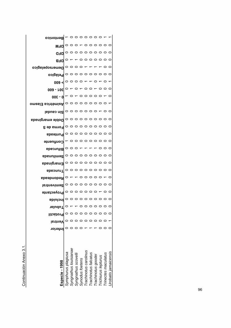
C
ontin
uaci
ón A
nexo
3.1
.
Es
pec
ie -
199
8
Inferior
Ventral
Protáctil
Tubular
Incluida
Proyectante
Semiventral
Redondeada
Truncada
Emarginada
Semilunada
Bifurcada
Confluente
Punteada
Forma de S
Doble emarginada
Sin caudal
Asimétrica Elasmo
0 - 300
301 - 600
> 600
Pelágico
Demersopelagico
DFB
DFD
DFM
Bentonico
Sym
phur
us p
lagi
usa
00
00
00
00
00
00
1 0
00
00
10
00
00
00
1 S
yngn
athu
s lo
uisi
anae
0
00
10
00
10
00
0 0
00
00
00
10
00
10
00
Syn
gnat
hus
scov
elli
00
01
00
01
00
00
0 0
00
00
10
00
01
00
0 S
ynod
us fo
eten
s 0
00
00
00
00
00
1 0
00
00
00
10
00
00
10
Trac
hino
tus
caro
linus
1
00
00
00
00
00
1 0
00
00
00
01
01
00
00
Trac
hino
tus
falc
atus
1
00
00
00
00
00
1 0
00
00
00
01
01
00
00
Trac
hino
tus
good
ei
10
00
00
00
00
01
0 0
00
00
01
00
10
00
0 Tr
ichi
urus
lept
urus
0
00
00
10
00
00
0 0
00
01
00
01
01
00
00
Trin
ecte
s m
acul
atus
0
00
00
00
10
00
0 0
00
00
01
00
00
00
01
Uro
batis
jam
aice
nsis
0
10
00
00
00
00
0 0
00
00
10
01
00
00
01
96

C
ontin
uaci
ón A
nexo
3.1
.
Es
pec
ie -
199
8
Marino
Mar-Anfídromo
Anádromo
Catádromo
Dulce
Dulce-Andrídromo
Oceanódromo
Aca
ntho
stra
cion
qua
dric
orni
s 1
00
00
00
Ach
irus
linea
tus
01
00
00
0A
ncho
a he
pset
us
01
00
00
0A
ncho
a m
itchi
lli 0
10
00
00
Arc
hosa
rgus
pro
bato
ceph
alus
0
10
00
00
Arc
hosa
rgus
rhom
boid
alis
0
10
00
00
Ario
psis
felis
0
10
00
00
Bag
re m
arin
us
01
00
00
0B
aird
iella
chr
ysou
ra
01
00
00
0B
aird
iella
ronc
hus
01
00
00
0B
athy
gobi
us s
opor
ator
1
00
00
00
Bre
voor
tia g
unte
ri 0
10
00
00
Cal
amus
pen
na
10
00
00
0C
aran
x cr
ysos
1
00
00
00
Car
anx
hipp
os
00
00
00
1C
atho
rops
mel
anop
us
00
00
10
0C
entro
pom
us p
aral
lelu
s 0
10
00
00
Cen
tropo
mus
poe
yi
01
00
00
0C
eten
grau
lis e
dent
ulus
0
10
00
00
Cha
etod
ipte
rus
fabe
r 0
00
00
01
Chi
lom
ycte
rus
scho
epfii
1
00
00
00
Chl
oros
com
brus
chr
ysur
us
01
00
00
0C
ichl
asom
a ur
opht
halm
um
00
00
01
0C
ithar
icht
hys
spilo
pter
us
01
00
00
0C
onod
on n
obili
s 1
00
00
00
Cyn
osci
on a
rena
rius
01
00
00
0C
ynos
cion
neb
ulos
us
01
00
00
0D
asya
tis s
abin
a 0
10
00
00
97

C
ontin
uaci
ón A
nexo
1.
Es
pec
ie -
199
8
Marino
Mar-Anfídromo
Anádromo
Catádromo
Dulce
Dulce-Andrídromo
Oceanódromo
Dia
pter
us a
urat
us
01
00
00
0D
iapt
erus
rhom
beus
0
10
00
00
Dor
osom
a pe
tene
nse
00
10
00
0E
lops
sau
rus
01
00
00
0E
pine
phel
us it
ajar
a 0
10
00
00
Etro
pus
cros
sotu
s 0
00
00
01
Euc
inos
tom
us a
rgen
teus
0
10
00
00
Euc
inos
tom
us g
ula
01
00
00
0E
ucin
osto
mus
mel
anop
teru
s 0
10
00
00
Eug
erre
s pl
umie
ri 0
10
00
00
Gob
ione
llus
ocea
nicu
s 0
10
00
00
Gym
noth
orax
sax
icol
a 1
00
00
00
Hae
mul
on a
urol
inea
tum
1
00
00
00
Hae
mul
on b
onar
iens
e 1
00
00
00
Hae
mul
on p
lum
ierii
1
00
00
00
Har
engu
la ja
guan
a 0
10
00
00
Hem
icar
anx
ambl
yrhy
nchu
s 1
00
00
00
Him
antu
ra s
chm
arda
e 1
00
00
00
Hip
poca
mpu
s er
ectu
s 1
00
00
00
Lago
ceph
alus
laev
igat
us
01
00
00
0La
godo
n rh
ombo
ides
0
10
00
00
Lobo
tes
surin
amen
sis
00
00
00
1Lu
tjanu
s an
alis
0
10
00
00
Lutja
nus
apod
us
01
00
00
0Lu
tjanu
s gr
iseu
s 0
10
00
00
Lutja
nus
syna
gris
1
00
00
00
Men
ticirr
hus
amer
ican
us
00
00
00
1M
entic
irrhu
s sa
xatil
is
01
00
00
0
98
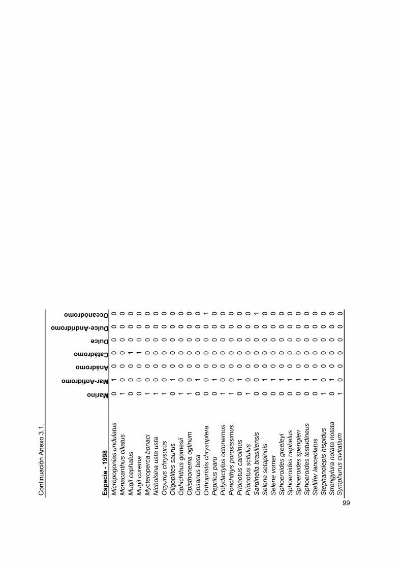
C
ontin
uaci
ón A
nexo
3.1
.
Es
pec
ie -
199
8
Marino
Mar-Anfídromo
Anádromo
Catádromo
Dulce
Dulce-Andrídromo
Oceanódromo
Mic
ropo
goni
as u
ndul
atus
0
10
00
00
Mon
acan
thus
cili
atus
1
00
00
00
Mug
il ce
phal
us
00
01
00
0M
ugil
cure
ma
00
01
00
0M
ycte
rope
rca
bona
ci
10
00
00
0N
icho
lsin
a us
ta u
sta
10
00
00
0O
cyur
us c
hrys
urus
1
00
00
00
Olig
oplit
es s
auru
s 0
10
00
00
Oph
icht
hus
gom
esii
10
00
00
0O
pist
hone
ma
oglin
um
10
00
00
0O
psan
us b
eta
01
00
00
0O
rthop
ristis
chr
ysop
tera
0
00
00
01
Pep
rilus
par
u 0
10
00
00
Pol
ydac
tylu
s oc
tone
mus
1
00
00
00
Por
icht
hys
poro
siss
imus
1
00
00
00
Prio
notu
s ca
rolin
us
01
00
00
0P
riono
tus
scitu
lus
10
00
00
0S
ardi
nella
bra
silie
nsis
0
00
00
01
Sel
ene
seta
pinn
is
01
00
00
0S
elen
e vo
mer
0
10
00
00
Sph
oero
ides
gre
eley
i 0
10
00
00
Sph
oero
ides
nep
helu
s 0
10
00
00
Sph
oero
ides
spe
ngle
ri 0
10
00
00
Sph
oero
ides
test
udin
eus
01
00
00
0S
telli
fer l
ance
olat
us
01
00
00
0S
teph
anol
epis
his
pidu
s 1
00
00
00
Stro
ngyl
ura
nota
ta n
otat
a 0
10
00
00
Sym
phur
us c
ivita
tium
1
00
00
00
99
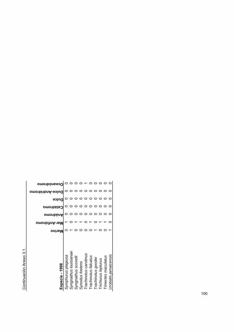
C
ontin
uaci
ón A
nexo
3.1
.
Es
pec
ie -
199
8
Marino
Mar-Anfídromo
Anádromo
Catádromo
Dulce
Dulce-Andrídromo
Oceanódromo
Sym
phur
us p
lagi
usa
01
00
00
0S
yngn
athu
s lo
uisi
anae
1
00
00
00
Syn
gnat
hus
scov
elli
01
00
00
0S
ynod
us fo
eten
s 0
10
00
00
Trac
hino
tus
caro
linus
0
00
00
01
Trac
hino
tus
falc
atus
0
10
00
00
Trac
hino
tus
good
ei
10
00
00
0Tr
ichi
urus
lept
urus
0
10
00
00
Trin
ecte
s m
acul
atus
0
10
00
00
Uro
batis
jam
aice
nsis
1
00
00
00
100

C
ont
inu
ació
n A
nexo
3.1
.
Es
pec
ie –
201
1
2 - 2.50
2.51 - 3.00
3.01 - 3.50
3.51 - 4.00
> 4.00
OGO
OHBFP
OHBSFP
OHP
OVO
Ictioinvertivoros
Piscivoros
Invertívoros
Omnívoros
Planctívoros
Anguiliforme
Compresiforme
Depresiforme A
Depresiforme B
Fusiforme
Globiforme
Sagitiforme
Teniforme
Otras Formas
Oblicua
Superior
Terminal
Aca
ntho
stra
cion
qua
dric
orni
s 0
01
00
00
01
00
01
00
00
00
01
00
00
01
Ach
irus
linea
tus
00
01
00
00
10
00
1 0
00
01
00
00
00
01
0A
lute
rus
scho
epfii
1
00
00
00
01
00
00
01
01
00
00
00
00
01
Anc
hoa
heps
etus
0
01
00
00
01
00
01
00
01
00
00
00
00
00
Anc
hoa
lyol
epis
0
01
00
00
01
00
01
00
01
00
00
00
00
00
Anc
hoa
mitc
hilli
00
10
00
00
10
00
1 0
00
10
00
00
00
00
0A
ncyl
opse
tta o
mm
ata
00
01
00
00
10
00
1 0
00
01
00
00
00
00
1A
rcho
sarg
us p
roba
toce
phal
us
00
10
00
00
10
00
1 0
00
10
00
00
00
00
0A
rcho
sarg
us rh
ombo
idal
is
00
10
00
00
10
00
1 0
00
10
00
00
00
00
0A
riops
is fe
lis
00
10
01
00
00
10
0 0
00
00
10
00
00
00
0B
agre
mar
inus
0
01
00
10
00
01
00
00
00
01
00
00
00
00
Bai
rdie
lla c
hrys
oura
0
00
10
00
01
00
01
00
01
00
00
00
00
00
Bai
rdie
lla ro
nchu
s 0
00
10
00
01
00
01
00
01
00
00
00
00
00
Car
anx
crys
os
00
01
00
00
10
10
0 0
00
10
00
00
00
00
0C
aran
x hi
ppos
0
00
10
00
01
01
00
00
01
00
00
00
00
00
Car
anx
latu
s 0
00
01
00
01
01
00
00
01
00
00
00
00
00
Car
anx
rube
r 0
00
01
00
01
01
00
00
01
00
00
00
00
00
Cat
horo
ps m
elan
opus
0
00
10
10
00
00
00
10
00
01
00
00
00
00
Cen
tropo
mus
par
alle
lus
00
00
10
10
00
10
0 0
00
10
00
00
00
00
0C
eten
grau
lis e
dent
ulus
1
00
00
00
01
00
00
01
01
00
00
00
00
00
Cha
etod
ipte
rus
fabe
r 0
01
00
00
01
00
00
10
01
00
00
00
00
01
Chi
lom
ycte
rus
scho
epfii
0
01
00
00
01
00
01
00
00
00
01
00
00
01
Chl
oros
com
brus
chr
ysur
us
00
01
00
00
10
10
0 0
00
10
00
00
00
00
0C
ichl
asom
a ur
opht
halm
um
00
01
01
00
00
10
0 0
00
10
00
00
00
00
0C
ithar
icht
hys
spilo
pter
us
00
01
00
00
10
00
0 1
00
01
00
00
00
00
1C
ynos
cion
are
nariu
s 0
00
01
00
01
00
01
00
01
00
00
00
00
00
Cyn
osci
on n
ebul
osus
0
00
10
00
01
00
01
00
01
00
00
00
00
00
Cyn
osci
on n
othu
s 0
00
01
00
01
00
01
00
01
00
00
00
00
00
Dac
tylo
pter
us v
olita
ns
00
01
00
00
10
00
1 0
00
00
10
00
00
00
0
101

C
ontin
uaci
ón A
nexo
3.1
.
Es
pec
ie –
201
1
2 - 2.50
2.51 - 3.00
3.01 - 3.50
3.51 - 4.00
> 4.00
OGO
OHBFP
OHBSFP
OHP
OVO
Ictioinvertivoros
Piscivoros
Invertívoros
Omnívoros
Planctívoros
Anguiliforme
Compresiforme
Depresiforme A
Depresiforme B
Fusiforme
Globiforme
Sagitiforme
Teniforme
Otras Formas
Oblicua
Superior
Terminal
Das
yatis
am
eric
ana
00
01
00
00
01
00
1
00
00
10
00
00
00
00
Das
yatis
sab
ina
00
10
00
00
01
00
1
00
00
10
00
00
00
00
Dia
pter
us a
urat
us
00
10
00
00
10
00
1
00
01
00
00
00
00
00
Dia
pter
us rh
ombe
us
00
10
00
00
10
00
1
00
01
00
00
00
00
00
Dip
lect
rum
biv
ittat
um
00
01
00
00
10
00
1
00
01
00
00
00
00
00
Dip
lect
rum
form
osum
0
00
01
00
01
00
0 1
0
00
10
00
00
00
00
0 D
oros
oma
anal
e 0
10
00
00
01
00
0 0
0
10
10
00
00
00
00
1 D
oros
oma
pete
nens
e 0
10
00
00
01
00
0 0
1
00
10
00
00
00
00
1 E
tropu
s cr
osso
tus
00
10
00
00
10
00
1
00
00
10
00
00
00
01
Euc
inos
tom
us a
rgen
teus
0
01
00
00
01
00
0 1
0
00
10
00
00
00
00
0 E
ucin
osto
mus
gul
a 0
01
00
00
01
00
0 1
0
00
10
00
00
00
00
0 E
uger
res
plum
ieri
00
10
00
00
10
00
1
00
01
00
00
00
00
00
Gob
ione
llus
ocea
nicu
s 0
01
00
00
10
00
0 0
1
00
00
01
00
00
00
0 G
ymno
thor
ax n
igro
mar
gina
tus
00
00
10
00
10
10
0
00
10
00
00
00
00
01
Gym
nura
mic
rura
0
00
10
00
00
10
0 1
0
00
01
00
00
00
00
0 H
aem
ulon
aur
olin
eatu
m
00
10
00
00
10
00
1
00
01
00
00
00
00
00
Hae
mul
on b
onar
iens
e 0
00
10
00
01
00
0 1
0
00
10
00
00
00
00
0 H
aem
ulon
plu
mie
rii
00
01
00
00
10
00
1
00
01
00
00
00
00
00
Har
engu
la ja
guan
a 0
01
00
00
01
00
0 1
0
00
10
00
00
00
00
1 H
emic
aran
x am
blyr
hync
hus
00
10
00
00
10
10
0
00
01
00
00
00
00
00
Hip
poca
mpu
s er
ectu
s 0
01
00
00
00
10
0 1
0
00
00
00
00
01
00
0 La
goce
phal
us la
evig
atus
0
00
01
00
01
01
0 0
0
00
00
00
10
00
00
1 La
godo
n rh
ombo
ides
0
00
10
00
01
00
0 1
0
00
10
00
00
00
00
0 Lu
tjanu
s gr
iseu
s 0
00
01
00
01
01
0 0
0
00
10
00
00
00
00
0 Lu
tjanu
s sy
nagr
is
00
01
00
00
10
10
0
00
01
00
00
00
00
00
Men
ticirr
hus
amer
ican
us
00
10
00
00
10
00
1
00
01
00
00
00
00
00
Men
ticirr
hus
saxa
tilis
0
00
10
00
01
00
0 1
0
00
10
00
00
00
00
0 M
icro
pogo
nias
furn
ieri
00
10
00
00
10
00
1
00
01
00
00
00
00
00
Mic
ropo
goni
as u
ndul
atus
0
01
00
00
01
00
0 1
0
00
10
00
00
00
00
0
102

C
ontin
uaci
ón A
nexo
3.1
.
Es
pec
ie –
201
1
2 - 2.50
2.51 - 3.00
3.01 - 3.50
3.51 - 4.00
> 4.00
OGO
OHBFP
OHBSFP
OHP
OVO
Ictioinvertivoros
Piscivoros
Invertívoros
Omnívoros
Planctívoros
Anguiliforme
Compresiforme
Depresiforme A
Depresiforme B
Fusiforme
Globiforme
Sagitiforme
Teniforme
Otras Formas
Oblicua
Superior
Terminal
Mon
acan
thus
cili
atus
0
10
00
00
01
00
0 0
1
00
10
00
00
00
00
1 M
ugil
cure
ma
10
00
00
00
10
00
0
10
00
00
10
00
00
01
Myc
tero
perc
a bo
naci
0
00
01
00
01
01
0 0
0
00
10
00
00
00
00
0 O
ligop
lites
sau
rus
00
01
00
00
10
10
0
00
01
00
00
00
00
00
Opi
stho
nem
a og
linum
0
01
00
00
01
00
0 1
0
00
10
00
00
00
00
1 O
psan
us b
eta
00
01
00
01
00
00
1
00
00
01
00
00
00
10
Orth
opris
tis c
hrys
opte
ra
00
01
00
00
10
00
1
00
01
00
00
00
00
00
Pep
rilus
par
u 0
00
10
00
01
01
0 0
0
00
10
00
00
00
00
1 P
olyd
acty
lus
octo
nem
us
00
01
00
00
10
00
0
10
01
00
00
00
00
00
Por
icht
hys
poro
siss
imus
0
00
10
00
10
01
0 0
0
00
00
10
00
00
01
0 P
riono
tus
caro
linus
0
00
01
00
01
01
0 0
0
00
00
10
00
00
00
0 P
riono
tus
mar
tis
00
01
00
00
10
10
0
00
00
01
00
00
00
00
Prio
notu
s pu
ncta
tus
00
01
00
00
10
10
0
00
00
01
00
00
00
00
Prio
notu
s ru
bio
00
01
00
00
10
10
0
00
00
01
00
00
00
00
Prio
notu
s sc
itulu
s 0
00
01
00
01
01
0 0
0
00
00
10
00
00
00
0 P
riono
tus
tribu
lus
00
01
00
00
10
10
0
00
00
01
00
00
00
00
Rhi
noba
tos
lent
igin
osus
0
00
10
00
00
10
0 1
0
00
01
00
00
00
00
0 S
corp
aena
bra
silie
nsis
0
00
10
00
01
01
0 0
0
00
10
00
00
00
00
0 S
corp
aena
plu
mie
ri 0
00
10
00
01
01
0 0
0
00
10
00
00
00
00
0 S
elen
e se
tapi
nnis
0
00
10
00
01
01
0 0
0
00
10
00
00
00
00
0 S
elen
e vo
mer
0
00
10
00
01
01
0 0
0
00
10
00
00
00
00
0 S
phoe
roid
es g
reel
eyi
00
10
00
00
10
00
1
00
00
00
01
00
00
01
Sph
oero
ides
mac
ulat
us
00
00
10
00
10
00
1
00
00
00
01
00
00
01
Sph
oero
ides
nep
helu
s 1
00
00
00
01
00
0 1
0
00
00
00
10
00
00
1 S
phoe
roid
es p
achy
gast
er
00
00
10
00
10
00
1
00
00
00
01
00
00
01
Sph
oero
ides
par
vus
00
10
00
00
10
00
1
00
00
00
01
00
00
01
Sph
oero
ides
spe
ngle
ri 0
01
00
00
01
00
0 1
0
00
00
00
10
00
00
1 S
phoe
roid
es te
stud
ineu
s 0
01
00
00
01
00
0 1
0
00
00
00
10
00
00
1 S
phyr
aena
bar
racu
da
00
00
10
00
10
01
0
00
00
00
00
10
00
00
103

C
ontin
uaci
ón A
nexo
3.1
.
Es
pec
ie –
201
1
2 - 2.50
2.51 - 3.00
3.01 - 3.50
3.51 - 4.00
> 4.00
OGO
OHBFP
OHBSFP
OHP
OVO
Ictioinvertivoros
Piscivoros
Invertívoros
Omnívoros
Planctívoros
Anguiliforme
Compresiforme
Depresiforme A
Depresiforme B
Fusiforme
Globiforme
Sagitiforme
Teniforme
Otras Formas
Oblicua
Superior
Terminal
Ste
llife
r lan
ceol
atus
0
00
10
00
01
00
0
1
00
01
00
00
00
00
00
Ste
phan
olep
is h
ispi
dus
01
00
00
00
10
00
1
0
00
10
00
00
00
00
1 S
yaci
um g
unte
ri 0
01
00
00
01
00
0
1
00
00
10
00
00
00
10
Sym
phur
us p
lagi
usa
01
00
00
00
10
00
1
0
00
01
00
00
00
00
1 S
yngn
athu
s fu
scus
0
01
00
00
00
10
0
1
00
10
00
00
00
00
00
Syn
gnat
hus
scov
elli
00
10
00
00
01
00
1
0
01
00
00
00
00
00
0 S
ynod
us fo
eten
s 0
00
01
00
01
00
1
0
00
00
00
00
10
01
00
Tric
hiur
us le
ptur
us
00
00
10
00
10
10
0
0
00
00
00
00
10
00
0 Tr
inec
tes
mac
ulat
us
01
00
00
00
10
00
1
0
00
01
00
00
00
00
1 U
roba
tis ja
mai
cens
is
00
01
00
00
01
10
0
0
00
01
00
00
00
00
0
104

C
ont
inu
ació
n A
nexo
3.1
.
Es
pec
ie -
201
1
Inferior
Ventral
Protáctil
Tubular
Incluida
Proyectante
Semiventral
Redondeada
Truncada
Emarginada
Semilunada
Bifurcada
Confluente
Punteada
Forma de S
Doble emarginada
Sin caudal
Asimétrica Elasmo
0 - 300
301 - 600
> 600
Pelágico
Demersopelagico
DFB
DFD
DFM
Bentonico
Aca
ntho
stra
cion
qua
dric
orni
s 0
00
00
00
10
00
0 0
0
00
00
01
00
00
01
0A
chiru
s lin
eatu
s 0
00
00
00
10
00
0 0
0
00
00
10
00
00
00
1A
lute
rus
scho
epfii
0
00
00
00
10
00
0 0
0
00
00
01
00
10
00
0A
ncho
a he
pset
us
00
10
00
00
00
01
0
00
00
01
00
10
00
00
Anc
hoa
lyol
epis
0
01
00
00
00
00
1 0
0
00
00
10
01
00
00
0A
ncho
a m
itchi
lli 0
01
00
00
00
00
1 0
0
00
00
10
01
00
00
0A
ncyl
opse
tta o
mm
ata
00
00
00
00
00
00
0
10
00
01
00
00
00
01
Arc
hosa
rgus
pro
bato
ceph
alus
1
00
00
00
00
00
1 0
0
00
00
01
00
00
01
0A
rcho
sarg
us rh
ombo
idal
is
10
00
00
00
00
01
0
00
00
00
10
00
00
10
Ario
psis
felis
1
00
00
00
00
00
1 0
0
00
00
00
10
01
00
0B
agre
mar
inus
1
00
00
00
00
00
1 0
0
00
00
00
10
01
00
0B
aird
iella
chr
ysou
ra
00
00
01
00
00
00
0
00
10
01
00
00
10
00
Bai
rdie
lla ro
nchu
s 0
00
00
10
00
00
0 0
0
01
00
01
00
01
00
0C
aran
x cr
ysos
0
00
00
10
00
00
1 0
0
00
00
00
10
10
00
0C
aran
x hi
ppos
0
00
00
10
00
00
1 0
0
00
00
00
10
10
00
0C
aran
x la
tus
00
00
01
00
00
01
0
00
00
00
01
01
00
00
Car
anx
rube
r 0
00
00
10
00
00
1 0
0
00
00
01
00
10
00
0C
atho
rops
mel
anop
us
10
00
00
00
00
01
0
00
00
01
00
01
00
00
Cen
tropo
mus
par
alle
lus
00
00
01
00
00
01
0
00
00
00
01
00
00
10
Cet
engr
aulis
ede
ntul
us
00
10
00
00
00
01
0
00
00
01
00
10
00
00
Cha
etod
ipte
rus
fabe
r 0
00
00
00
00
10
0 0
0
00
00
00
10
00
01
0C
hilo
myc
teru
s sc
hoep
fii
00
00
00
01
00
00
0
00
00
01
00
01
00
00
Chl
oros
com
brus
chr
ysur
us
00
00
01
00
00
01
0
00
00
00
01
10
00
00
Cic
hlas
oma
urop
htha
lmum
0
00
00
10
01
00
0 0
0
00
00
01
00
10
00
0C
ithar
icht
hys
spilo
pter
us
00
00
00
00
00
00
0
10
00
01
00
00
00
01
Cyn
osci
on a
rena
rius
00
00
01
00
00
00
0
00
10
00
01
00
10
00
Cyn
osci
on n
ebul
osus
0
00
00
10
00
10
0 0
0
00
00
00
10
01
00
0C
ynos
cion
not
hus
00
00
01
00
00
00
0
01
00
00
10
00
10
00
105

C
ontin
uaci
ón A
nexo
3.1
.
Es
pec
ie -
201
1
Inferior
Ventral
Protáctil
Tubular
Incluida
Proyectante
Semiventral
Redondeada
Truncada
Emarginada
Semilunada
Bifurcada
Confluente
Punteada
Forma de S
Doble emarginada
Sin caudal
Asimétrica Elasmo
0 - 300
301 - 600
> 600
Pelágico
Demersopelagico
DFB
DFD
DFM
Bentonico
Dac
tylo
pter
us v
olita
ns
10
00
00
00
01
00
0
0
00
00
01
00
01
00
0 D
asya
tis a
mer
ican
a 0
10
00
00
00
00
0
0
00
01
00
01
00
00
01
Das
yatis
sab
ina
01
00
00
00
00
00
0
0
00
10
00
10
00
00
1 D
iapt
erus
aur
atus
0
01
00
00
00
00
1
0
00
00
00
10
00
10
00
Dia
pter
us rh
ombe
us
00
10
00
00
00
01
0
0
00
00
01
00
01
00
0 D
iple
ctru
m b
ivitt
atum
0
00
00
10
00
10
0
0
00
00
01
00
00
10
00
Dip
lect
rum
form
osum
0
00
00
10
00
10
0
0
00
00
01
00
00
10
00
Dor
osom
a an
ale
00
00
00
00
00
01
0
0
00
00
10
01
00
00
0 D
oros
oma
pete
nens
e 0
00
00
00
00
00
1
0
00
00
01
00
10
00
00
Etro
pus
cros
sotu
s 0
00
00
00
00
00
0
0
10
00
01
00
00
00
01
Euc
inos
tom
us a
rgen
teus
0
01
00
00
00
00
1
0
00
00
01
00
00
10
00
Euc
inos
tom
us g
ula
00
10
00
00
00
01
0
0
00
00
10
00
01
00
0 E
uger
res
plum
ieri
00
10
00
00
00
01
0
0
00
00
01
00
01
00
0 G
obio
nellu
s oc
eani
cus
00
00
10
01
00
00
0
0
00
00
10
00
00
00
1 G
ymno
thor
ax n
igro
mar
gina
tus
00
00
00
00
00
00
1
0
00
00
00
10
00
10
0 G
ymnu
ra m
icru
ra
01
00
00
00
00
00
0
0
00
10
00
10
00
00
1 H
aem
ulon
aur
olin
eatu
m
00
00
01
00
00
01
0
0
00
00
10
00
00
01
0 H
aem
ulon
bon
arie
nse
00
00
01
00
00
01
0
0
00
00
01
00
00
01
0 H
aem
ulon
plu
mie
rii
00
00
01
00
00
01
0
0
00
00
01
00
00
01
0 H
aren
gula
jagu
ana
00
00
00
00
00
01
0
0
00
00
10
01
00
00
0 H
emic
aran
x am
blyr
hync
hus
00
00
01
00
00
01
0
0
00
00
01
01
00
00
0 H
ippo
cam
pus
erec
tus
00
01
00
00
00
00
0
0
00
10
10
00
00
01
0 La
goce
phal
us la
evig
atus
0
00
00
00
00
01
0
0
00
00
00
01
10
00
00
Lago
don
rhom
boid
es
10
00
00
00
00
01
0
0
00
00
01
00
00
01
0 Lu
tjanu
s gr
iseu
s 0
00
00
10
00
01
0
0
00
00
00
01
00
00
10
Lutja
nus
syna
gris
0
00
00
10
00
01
0
0
00
00
00
01
00
00
10
Men
ticirr
hus
amer
ican
us
00
00
00
10
00
00
0
0
10
00
01
00
01
00
0 M
entic
irrhu
s sa
xatil
is
00
00
00
10
00
00
0
0
10
00
01
00
01
00
0
106
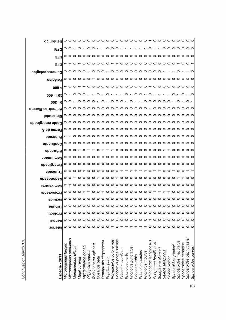
C
ontin
uaci
ón A
nexo
3.1
.
Es
pec
ie -
201
1
Inferior
Ventral
Protáctil
Tubular
Incluida
Proyectante
Semiventral
Redondeada
Truncada
Emarginada
Semilunada
Bifurcada
Confluente
Punteada
Forma de S
Doble emarginada
Sin caudal
Asimétrica Elasmo
0 - 300
301 - 600
> 600
Pelágico
Demersopelagico
DFB
DFD
DFM
Bentonico
Mic
ropo
goni
as fu
rnie
ri 0
00
00
01
00
00
00
1
00
00
00
10
01
00
0M
icro
pogo
nias
und
ulat
us
00
00
00
10
00
00
0 1
0
00
00
10
00
10
00
Mon
acan
thus
cili
atus
0
00
00
00
10
00
00
0
00
00
10
00
00
01
0M
ugil
cure
ma
00
00
00
00
00
01
0 0
0
00
00
01
00
10
00
Myc
tero
perc
a bo
naci
0
00
00
10
01
00
00
0
00
00
00
10
00
01
0O
ligop
lites
sau
rus
00
00
01
00
00
01
0 0
0
00
00
10
01
00
00
Opi
stho
nem
a og
linum
0
00
00
00
00
00
10
0
00
00
01
01
00
00
0O
psan
us b
eta
00
00
00
01
00
00
0 0
0
00
01
00
00
00
10
Orth
opris
tis c
hrys
opte
ra
00
00
01
00
00
01
0 0
0
00
00
10
00
00
10
Pep
rilus
par
u 0
00
00
00
00
00
10
0
00
00
10
00
10
00
0P
olyd
acty
lus
octo
nem
us
10
00
00
00
00
01
0 0
0
00
00
10
00
10
00
Por
icht
hys
poro
siss
imus
0
00
00
00
10
00
00
0
00
00
01
00
01
00
0P
riono
tus
caro
linus
1
00
00
00
01
00
00
0
00
00
01
00
00
01
0P
riono
tus
mar
tis
10
00
00
00
10
00
0 0
0
00
01
00
00
00
10
Prio
notu
s pu
ncta
tus
10
00
00
00
10
00
0 0
0
00
00
10
00
00
10
Prio
notu
s ru
bio
10
00
00
00
10
00
0 0
0
00
01
00
00
00
10
Prio
notu
s sc
itulu
s 1
00
00
00
01
00
00
0
00
00
10
00
00
01
0P
riono
tus
tribu
lus
10
00
00
00
10
00
0 0
0
00
00
10
00
00
10
Rhi
noba
tos
lent
igin
osus
0
10
00
00
00
00
00
0
00
01
00
10
00
00
1S
corp
aena
bra
silie
nsis
0
00
00
10
01
00
00
0
00
00
01
00
00
01
0S
corp
aena
plu
mie
ri 0
00
00
10
01
00
00
0
00
00
01
00
00
01
0S
elen
e se
tapi
nnis
0
00
00
10
00
00
10
0
00
00
01
00
10
00
0S
elen
e vo
mer
0
00
00
10
00
00
10
0
00
00
01
00
10
00
0S
phoe
roid
es g
reel
eyi
00
00
00
00
10
00
0 0
0
00
01
00
01
00
00
Sph
oero
ides
mac
ulat
us
00
00
00
01
00
00
0 0
0
00
00
10
00
10
00
Sph
oero
ides
nep
helu
s 0
00
00
00
10
00
00
0
00
00
10
00
10
00
0S
phoe
roid
es p
achy
gast
er
00
00
00
00
10
00
0 0
0
00
00
10
01
00
00
Sph
oero
ides
par
vus
00
00
00
00
10
00
0 0
0
00
01
00
00
10
00
107

C
ontin
uaci
ón A
nexo
3.1
.
Es
pec
ie -
201
1
Inferior
Ventral
Protáctil
Tubular
Incluida
Proyectante
Semiventral
Redondeada
Truncada
Emarginada
Semilunada
Bifurcada
Confluente
Punteada
Forma de S
Doble emarginada
Sin caudal
Asimétrica Elasmo
0 - 300
301 - 600
> 600
Pelágico
Demersopelagico
DFB
DFD
DFM
Bentonico
Sph
oero
ides
spe
ngle
ri 0
0
00
00
01
00
00
0
0
00
00
10
00
10
00
0S
phoe
roid
es te
stud
ineu
s 0
0
00
00
01
00
00
0
0
00
00
01
00
10
00
0S
phyr
aena
bar
racu
da
0
00
00
10
00
00
10
0
0
00
00
01
10
00
00
Ste
llife
r lan
ceol
atus
0
0
00
01
00
00
00
0
1
00
00
10
00
01
00
0S
teph
anol
epis
his
pidu
s 0
0
00
00
01
00
00
0
0
00
00
10
00
01
00
0S
yaci
um g
unte
ri 0
0
00
00
00
00
00
0
0
01
00
10
00
00
00
1S
ymph
urus
pla
gius
a 0
0
00
00
00
00
00
1
0
00
00
10
00
00
00
1S
yngn
athu
s fu
scus
0
0
01
00
01
00
00
0
0
00
00
01
00
01
00
0S
yngn
athu
s sc
ovel
li 0
0
01
00
01
00
00
0
0
00
00
10
00
01
00
0S
ynod
us fo
eten
s 0
0
00
00
00
00
01
0
0
00
00
01
00
00
01
0Tr
ichi
urus
lept
urus
0
0
00
01
00
00
00
0
0
00
10
00
10
10
00
0Tr
inec
tes
mac
ulat
us
0
00
00
00
10
00
00
0
0
00
01
00
00
00
01
Uro
batis
jam
aice
nsis
0
1
00
00
00
00
00
0
0
00
01
00
10
00
00
1
108

C
ont
inu
ació
n A
nexo
3.1
.
Es
pec
ie -
201
1
Marino
Mar-Anfídromo
Anádromo
Catádromo
Dulce
Dulce-Andrídromo
Oceanódromo
Aca
ntho
stra
cion
qua
dric
orni
s 1
00
00
00
Ach
irus
linea
tus
01
00
00
0A
lute
rus
scho
epfii
1
00
00
00
Anc
hoa
heps
etus
0
10
00
00
Anc
hoa
lyol
epis
1
00
00
00
Anc
hoa
mitc
hilli
01
00
00
0A
ncyl
opse
tta o
mm
ata
10
00
00
0A
rcho
sarg
us p
roba
toce
phal
us
01
00
00
0A
rcho
sarg
us rh
ombo
idal
is
01
00
00
0A
riops
is fe
lis
01
00
00
0B
agre
mar
inus
0
10
00
00
Bai
rdie
lla c
hrys
oura
0
10
00
00
Bai
rdie
lla ro
nchu
s 0
10
00
00
Car
anx
crys
os
10
00
00
0C
aran
x hi
ppos
0
00
00
01
Car
anx
latu
s 0
10
00
00
Car
anx
rube
r 0
00
00
01
Cat
horo
ps m
elan
opus
0
00
01
00
Cen
tropo
mus
par
alle
lus
01
00
00
0C
eten
grau
lis e
dent
ulus
0
10
00
00
Cha
etod
ipte
rus
fabe
r 0
00
00
01
Chi
lom
ycte
rus
scho
epfii
1
00
00
00
Chl
oros
com
brus
chr
ysur
us
01
00
00
0C
ichl
asom
a ur
opht
halm
um
00
00
01
0C
ithar
icht
hys
spilo
pter
us
01
00
00
0C
ynos
cion
are
nariu
s 0
10
00
00
Cyn
osci
on n
ebul
osus
0
10
00
00
Cyn
osci
on n
othu
s 0
10
00
00
109

C
ontin
uaci
ón A
nexo
3.1
.
Es
pec
ie -
201
1
Marino
Mar-Anfídromo
Anádromo
Catádromo
Dulce
Dulce-Andrídromo
Oceanódromo
Dac
tylo
pter
us v
olita
ns
01
00
00
0D
asya
tis a
mer
ican
a 0
10
00
00
Das
yatis
sab
ina
01
00
00
0D
iapt
erus
aur
atus
0
10
00
00
Dia
pter
us rh
ombe
us
01
00
00
0D
iple
ctru
m b
ivitt
atum
1
00
00
00
Dip
lect
rum
form
osum
1
00
00
00
Dor
osom
a an
ale
00
00
01
0D
oros
oma
pete
nens
e 0
01
00
00
Etro
pus
cros
sotu
s 0
00
00
01
Euc
inos
tom
us a
rgen
teus
0
10
00
00
Euc
inos
tom
us g
ula
01
00
00
0E
uger
res
plum
ieri
01
00
00
0G
obio
nellu
s oc
eani
cus
01
00
00
0G
ymno
thor
ax n
igro
mar
gina
tus
10
00
00
0G
ymnu
ra m
icru
ra
01
00
00
0H
aem
ulon
aur
olin
eatu
m
10
00
00
0H
aem
ulon
bon
arie
nse
10
00
00
0H
aem
ulon
plu
mie
rii
10
00
00
0H
aren
gula
jagu
ana
01
00
00
0H
emic
aran
x am
blyr
hync
hus
10
00
00
0H
ippo
cam
pus
erec
tus
10
00
00
0La
goce
phal
us la
evig
atus
0
10
00
00
Lago
don
rhom
boid
es
01
00
00
0Lu
tjanu
s gr
iseu
s 0
10
00
00
Lutja
nus
syna
gris
1
00
00
00
Men
ticirr
hus
amer
ican
us
00
00
00
1M
entic
irrhu
s sa
xatil
is
01
00
00
0
110

C
ontin
uaci
ón A
nexo
3.1
.
Es
pec
ie -
201
1
Marino
Mar-Anfídromo
Anádromo
Catádromo
Dulce
Dulce-Andrídromo
Oceanódromo
Mic
ropo
goni
as fu
rnie
ri 0
00
00
01
Mic
ropo
goni
as u
ndul
atus
0
10
00
00
Mon
acan
thus
cili
atus
1
00
00
00
Mug
il cu
rem
a 0
00
10
00
Myc
tero
perc
a bo
naci
1
00
00
00
Olig
oplit
es s
auru
s 0
10
00
00
Opi
stho
nem
a og
linum
1
00
00
00
Ops
anus
bet
a 0
10
00
00
Orth
opris
tis c
hrys
opte
ra
00
00
00
1P
epril
us p
aru
01
00
00
0P
olyd
acty
lus
octo
nem
us
10
00
00
0P
oric
hthy
s po
rosi
ssim
us
10
00
00
0P
riono
tus
caro
linus
0
10
00
00
Prio
notu
s m
artis
0
10
00
00
Prio
notu
s pu
ncta
tus
10
00
00
0P
riono
tus
rubi
o 0
10
00
00
Prio
notu
s sc
itulu
s 1
00
00
00
Prio
notu
s tri
bulu
s 1
00
00
00
Rhi
noba
tos
lent
igin
osus
1
00
00
00
Sco
rpae
na b
rasi
liens
is
10
00
00
0S
corp
aena
plu
mie
ri 1
00
00
00
Sel
ene
seta
pinn
is
01
00
00
0S
elen
e vo
mer
0
10
00
00
Sph
oero
ides
gre
eley
i 0
10
00
00
Sph
oero
ides
mac
ulat
us
01
00
00
0S
phoe
roid
es n
ephe
lus
01
00
00
0S
phoe
roid
es p
achy
gast
er
10
00
00
0S
phoe
roid
es p
arvu
s 0
10
00
00
111

C
ontin
uaci
ón A
nexo
3.1
.
Es
pec
ie -
201
1
Marino
Mar-Anfídromo
Anádromo
Catádromo
Dulce
Dulce-Andrídromo
Oceanódromo
Sph
oero
ides
spe
ngle
ri 0
10
00
00
Sph
oero
ides
test
udin
eus
01
00
00
0S
phyr
aena
bar
racu
da
01
00
00
0S
telli
fer l
ance
olat
us
01
00
00
0S
teph
anol
epis
his
pidu
s 1
00
00
00
Sya
cium
gun
teri
10
00
00
0S
ymph
urus
pla
gius
a 0
10
00
00
Syn
gnat
hus
fusc
us
01
00
00
0S
yngn
athu
s sc
ovel
li 0
10
00
00
Syn
odus
foet
ens
01
00
00
0Tr
ichi
urus
lept
urus
0
10
00
00
Trin
ecte
s m
acul
atus
0
10
00
00
Uro
batis
jam
aice
nsis
1
00
00
00
112

113
Anexo 3.2. Bloques de equivalencia funcional para el elenco sistemático de peces de la Laguna de Términos para los tres periodos evaluados.
A-1980 B-1980 C-1980
Acanthostracion quadricornis Achirus lineatus Anchoa hepsetus Aluterus schoepfii Citharichthys spilopterus Anchoa lamprotaenia Ancylopsetta ommata Dasyatis hastata Anchoa mitchilli Bothus ocellatus Dasyatis sabina Bairdiella chrysoura Chilomycterus schoepfii Etropus crossotus Cetengraulis edentulus Nicholsina usta usta Gobionellus oceanicus Chriodorus atherinoides Sphoeroides greeleyi Hippocampus erectus Diapterus rhombeus Sphoeroides nephelus Opsanus beta Eucinostomus argenteus Sphoeroides spengleri Symphurus plagiusa Eucinostomus gula Sphoeroides testudineus Syngnathus scovelli Eucinostomus melanopterus Stephanolepis hispidus Trinectes maculatus Eugerres plumieri
F-1980 E-1980 Harengula jaguana
Bairdiella ronchus Ariopsis felis Stellifer lanceolatus
Caranx hippos Bagre marinus D-1980
Chaetodipterus faber Centropomus undecimalis Archosargus probatocephalusCichlasoma urophthalmum Chloroscombrus chrysurus Archosargus rhomboidalis Cynoscion arenarius Lagocephalus laevigatus Menticirrhus americanus Cynoscion nebulosus Lutjanus analis Micropogonias undulatus Cynoscion nothus Lutjanus griseus Odontoscion dentex Haemulon bonariense Trichiurus lepturus Opisthonema oglinum
Haemulon plumierii G-1980 Syngnathus louisianae
Menticirrhus saxatilis Cathorops melanopus H-1980
Oligoplites saurus Prionotus beanii Lutjanus synagris Orthopristis chrysoptera Prionotus carolinus Ophichthus gomesii Polydactylus octonemus Prionotus punctatus Porichthys porosissimus Selene vomer Prionotus scitulus Scorpaena plumieri Synodus foetens Prionotus tribulus Urobatis jamaicensis

114
Continuación Anexo 3.2.
A-1998 B-1998 F-1998
Acanthostracion quadricornis Achirus lineatus Bairdiella ronchus Chilomycterus schoepfii Bathygobius soporator Cynoscion arenarius Etropus crossotus Citharichthys spilopterus Cynoscion nebulosus Hippocampus erectus Dasyatis sabina Haemulon bonariense Monacanthus ciliatus Gobionellus oceanicus Haemulon plumierii Nicholsina usta usta Himantura schmardae Hemicaranx amblyrhynchus Sphoeroides greeleyi Opsanus beta Lagodon rhomboides
Sphoeroides nephelus D-1998 Ocyurus chrysurus Sphoeroides spengleri Archosargus probatocephalus Oligoplites saurus Stephanolepis hispidus Archosargus rhomboidalis Orthopristis chrysoptera Symphurus civitatium Calamus penna Polydactylus octonemus Symphurus plagiusa Conodon nobilis Selene setapinnis Syngnathus scovelli Diapterus auratus Selene vomer Trinectes maculatus Diapterus rhombeus Synodus foetens
E-1998 Eugerres plumieri Trachinotus carolinus Ariopsis felis Haemulon aurolineatum Trachinotus falcatus Bagre marinus Menticirrhus americanus Trachinotus goodei
Caranx crysos Menticirrhus saxatilis G-1998
Caranx hippos Micropogonias undulatus Cathorops melanopus Centropomus parallelus Opisthonema oglinum Chaetodipterus faber Centropomus poeyi Sphoeroides testudineus Mugil cephalus Chloroscombrus chrysurus Syngnathus louisianae Mugil curema
Elops saurus C-1998 Peprilus paru
Epinephelus itajara Anchoa hepsetus H-1998
Lagocephalus laevigatus Anchoa mitchilli Cichlasoma urophthalmum Lobotes surinamensis Bairdiella chrysoura Gymnothorax saxicola Lutjanus analis Brevoortia gunteri Lutjanus synagris Lutjanus apodus Cetengraulis edentulus Mycteroperca bonaci Lutjanus griseus Dorosoma petenense Ophichthus gomesii Prionotus carolinus Eucinostomus argenteus Porichthys porosissimus Strongylura notata notata Eucinostomus gula Prionotus scitulus Trichiurus lepturus Eucinostomus melanopterus Urobatis jamaicensis
Harengula jaguana Sardinella brasiliensis Stellifer lanceolatus

115
Continuación Anexo 3.2.
A-2011 C-2011 B-2011
Acanthostracion quadricornis Bairdiella chrysoura Achirus lineatus Anchoa hepsetus Dactylopterus volitans Ancylopsetta ommata Anchoa lyolepis Diapterus auratus Chilomycterus schoepfii Anchoa mitchilli Diapterus rhombeus Citharichthys spilopterus Cetengraulis edentulus Eucinostomus argenteus Etropus crossotus Diplectrum formosum Eucinostomus gula Gobionellus oceanicus Dorosoma anale Eugerres plumieri Hippocampus erectus Dorosoma petenense Menticirrhus americanus Opsanus beta Haemulon aurolineatum Menticirrhus saxatilis Sphoeroides greeleyi Harengula jaguana Micropogonias furnieri Sphoeroides nephelus Monacanthus ciliatus Micropogonias undulatus Sphoeroides parvus Mugil curema Sphoeroides maculatus Sphoeroides spengleri Opisthonema oglinum Sphoeroides testudineus Syacium gunteri Sphoeroides pachygaster Stellifer lanceolatus Symphurus plagiusa Stephanolepis hispidus Syngnathus fuscus Syngnathus scovelli
F-2011 G-2011 Trinectes maculatus
Aluterus schoepfii Cathorops melanopus E-2011
Archosargus probatocephalus Porichthys porosissimus Ariopsis felis Archosargus rhomboidalis Prionotus carolinus Bagre marinus Bairdiella ronchus Prionotus martis Caranx crysos Chaetodipterus faber Prionotus punctatus Caranx hippos Cynoscion arenarius Prionotus rubio Caranx latus Cynoscion nebulosus Prionotus scitulus Caranx ruber
Cynoscion nothus H-2011 Centropomus parallelus Diplectrum bivittatum Cichlasoma urophthalmum Chloroscombrus chrysurus
Haemulon bonariense Gymnothorax nigromarginatus Lagocephalus laevigatus
Haemulon plumierii Lutjanus synagris Lutjanus griseus Hemicaranx amblyrhynchus Scorpaena brasiliensis Oligoplites saurus Lagodon rhomboides Scorpaena plumieri Peprilus paru Orthopristis chrysoptera Urobatis jamaicensis Selene setapinnis
Polydactylus octonemus D-2011 Selene vómer
Synodus foetens Dasyatis americana Sphyraena barracuda
Dasyatis sabina Trichiurus lepturus Gymnura micrura Rhinobatos lentiginosus

A
nexo
4.1
. Mat
riz d
epr
eda
dor
pres
a q
ue r
epre
sent
a la
die
ta d
e lo
s gr
upo
s en
el m
ode
lo tr
ófic
o de
la L
agun
a de
Tér
min
os p
ara
cada
uno
de
los
peri
odos
.
1980
P
resa
\ D
epre
dad
or
1 2
3 4
5 6
7 8
9 10
11
12
13
14
15
16
17
1 D
elfin
es
- -
- -
- -
- -
- -
- -
- -
- -
-
2 A
ves
Mar
inas
-
- -
- -
- -
- -
- -
- -
- -
- -
3 T
ortu
gas
Mar
inas
-
- -
- -
- -
- -
- -
- -
- -
- -
4 A
guja
s 0.
00
- -
- -
- 0.
01
0.00
-
0.02
0.
00
- 0.
00
- 0.
00
- -
5 A
ncho
veta
s 0.
00
0.01
-
- 0.
00
- -
0.00
0.
00
0.03
0.
00
- 0.
00
- -
- 0.
00
6 A
ngui
las
- -
- -
- 0.
01
- -
- -
0.00
-
- -
0.00
-
-
7 B
agre
s 0.
07
0.09
0.
01
- -
- -
- -
0.37
-
- 0.
00
- -
- -
8 B
arbu
dos
0.02
-
- -
- -
- -
- 0.
25
- -
- -
0.00
-
-
9 C
intil
las
0.00
-
- -
- -
- -
0.00
-
- -
0.00
-
- -
-
10
Cor
vin
as
0.01
0.
04
- -
- -
- -
0.01
0.
14
0.04
-
- -
- -
-
11
Igua
nas
-
0.01
-
- -
- -
- 0.
00
- 0.
00
- 0.
00
- 0.
00
- -
12
Isab
elita
s -
- -
- -
- 0.
02
- 0.
00
- -
- -
- -
- -
13
Jure
les
0.01
-
- -
- -
- 0.
03
- -
- -
- -
- -
-
14
Lisa
s -
- -
0.00
-
- 0.
01
- -
0.02
-
- 0.
00
- -
0.01
-
15
Mer
os
0.00
0.
00
- -
- -
- -
0.00
-
- -
- -
0.00
-
-
16
Moj
arra
s
0.01
0.
23
- -
- -
- -
- -
- -
0.03
-
- -
-
17
Moj
arra
s M
exic
anas
-
- -
- -
- 0.
03
- -
- -
- -
- -
- -
18
Par
gos
- 0.
03
- -
- 0.
04
- -
0.00
-
- -
- -
- -
-
19
Pec
es G
lob
o 0.
03
- 0.
03
- -
- 0.
01
- -
- -
- -
- 0.
06
- -
20
Pec
es P
lano
s -
- -
- -
- -
- -
0.14
-
- -
- -
- -
21
Pec
es R
oca
-
- -
- -
- -
- 0.
00
- -
- -
- 0.
00
- -
22
Pej
esap
os
0.03
-
- -
- -
- -
- -
- -
- -
- -
-
23
Per
icos
-
- -
- -
- -
- -
- -
- -
- 0.
01
- -
24
Ra
yas
- -
- -
- -
- -
- -
- -
- -
0.02
-
-
25
Rob
alos
-
- -
- -
- -
- -
- -
- 0.
04
- -
- -
26
Ron
cos
0.01
0.
03
- -
- -
- -
- -
- -
- -
- -
-
27
Sar
dina
s 0.
00
0.00
-
- -
- -
0.00
0.
00
0.01
0.
00
- 0.
00
- -
- 0.
00
28
Sar
gos
0.06
-
- -
- -
- 0.
08
- 0.
62
- -
0.02
-
- -
-
29
Jaib
as
- -
0.00
-
0.00
0.
02
0.00
0.
01
0.00
0.
01
- -
0.00
-
0.04
-
0.01
30
Cam
arón
Bla
nco
-
- 0.
04
- -
- 0.
07
0.52
0.
00
0.40
0.
01
- 0.
04
0.04
0.
02
- -
31
Cam
arón
Caf
é -
- 0.
04
- -
- 0.
03
0.04
0.
00
0.46
0.
01
- 0.
01
0.03
0.
00
- -
116

C
ont
inu
ació
n A
nexo
4.1
.
1980
P
resa
\ D
epre
dad
or
1 2
3 4
5 6
7 8
9 10
11
12
13
14
15
16
17
32
Cam
arón
Ros
ado
-
- 0.
07
- -
- 0.
03
0.04
0.
00
0.75
0.
01
- 0.
01
0.03
0.
00
- -
33
Mol
usco
s -
- 0.
02
0.05
0.
00
- 0.
11
0.03
-
- 0.
01
0.16
0.
04
0.07
-
- 0.
20
34
Equ
inod
erm
os
0.01
-
0.06
-
- 0.
08
0.10
-
0.01
-
- 0.
98
- -
0.03
-
-
35
Mic
rocr
ustá
ceo
s 0.
02
- 0.
09
0.05
0.
16
0.11
0.
36
0.38
-
1.32
0.
03
- 0.
17
0.29
0.
00
0.24
0.
38
36
Pol
ique
tos
- -
- 0.
03
- 0.
15
0.05
0.
12
- 0.
11
0.01
0.
25
0.05
0.
19
0.00
1.
92
-
37
Mei
obe
ntos
-
- 0.
02
0.03
0.
00
- 0.
36
0.25
-
0.61
-
0.23
-
0.29
-
0.42
0.
00
38
Zoo
plan
cto
n -
- -
0.12
0.
08
- 0.
36
0.03
-
- 0.
02
- -
0.07
-
0.19
-
39
Pas
tos
Mar
ino
s -
- 0.
36
- 0.
01
- 0.
11
- -
0.14
0.
02
0.21
-
- -
0.10
0.
06
40
Fito
pla
ncto
n
- -
- -
0.05
-
- -
- -
0.00
-
0.02
0.
40
- -
-
41
Det
ritos
-
- -
- -
- 1.
68
- -
0.06
-
- 0.
04
0.60
-
0.32
0.
14
117

C
ont
inu
ació
n A
nexo
4.1
.
1980
P
resa
\ D
epre
dad
or
18
19
20
21
22
23
24
25
26
27
28
29
30
31
32
33
34
1 D
elfin
es
- -
- -
- -
- -
- -
- -
- -
- -
-
2 A
ves
Mar
inas
-
- -
- -
- -
- -
- -
- -
- -
- -
3 T
ortu
gas
Mar
inas
-
- -
- -
- -
- -
- -
- -
- -
- -
4 A
guja
s 0.
00
- -
- -
- -
- -
0.00
-
- -
- -
- -
5 A
ncho
veta
s -
- -
- 0.
01
- -
0.00
-
- -
- -
- -
- -
6 A
ngui
las
- -
- -
0.01
-
- -
- -
- -
- -
- -
-
7 B
agre
s -
- -
- -
- -
0.00
0.
01
- -
- -
- -
- -
8 B
arbu
dos
- -
- -
- -
- -
- -
- -
- -
- -
-
9 C
intil
las
- -
- -
- -
- -
- -
- -
- -
- -
-
10
Cor
vin
as
- -
- -
- -
- 0.
00
0.05
-
- -
- -
- -
-
11
Igua
nas
0.
00
- -
- -
- -
- -
- -
- -
- -
- -
12
Isab
elita
s 0.
03
- -
- -
- -
- -
- -
- -
- -
- -
13
Jure
les
- -
- -
- -
- -
- -
- -
- -
- -
-
14
Lisa
s 0.
00
- -
- -
- 0.
01
0.00
0.
01
- 0.
07
0.01
-
- -
- -
15
Mer
os
0.00
-
- -
- -
- -
- -
- -
- -
- -
-
16
Moj
arra
s -
- -
- 0.
05
- -
- -
0.01
-
- -
- -
- -
17
Moj
arra
s M
exic
anas
-
- -
- -
- -
0.02
-
- -
- -
- -
- -
18
Par
gos
- -
- -
- -
- 0.
00
- -
- -
- -
- -
-
19
Pec
es G
lob
o 0.
13
- -
- -
- -
- -
- -
- -
- -
- -
20
Pec
es P
lano
s -
- -
0.02
-
- -
- 0.
00
- -
- -
- -
- -
21
Pec
es R
oca
0.
00
- -
0.00
-
- -
- -
- -
- -
- -
- -
22
Pej
esap
os
- -
- 0.
01
- -
- -
0.02
-
- -
- -
- -
-
23
Per
icos
0.
03
- -
- -
- -
- -
- -
- -
- -
- -
24
Ra
yas
- -
- -
0.03
-
- -
- -
- -
- -
- -
-
25
Rob
alos
-
- -
- -
- -
- -
- -
- -
- -
- -
26
Ron
cos
0.06
-
- -
- -
- -
- -
- -
- -
- -
-
27
Sar
dina
s 0.
00
- -
- -
- -
0.00
-
0.00
-
- -
- -
- -
28
Sar
gos
- -
- -
0.05
-
- -
0.07
-
- -
- -
- -
-
29
Jaib
as
0.02
-
0.03
0.
09
0.00
0.
14
- 0.
01
0.01
-
- -
- -
- -
-
30
Cam
arón
Bla
nco
0.
13
- -
0.39
-
- 0.
25
0.06
0.
10
- -
0.04
0.
23
0.12
0.
20
- 0.
23
31
Cam
arón
Caf
é 0.
04
- -
0.02
-
- 0.
17
0.00
0.
03
- -
0.00
0.
02
0.01
0.
01
- -
32
Cam
arón
Ros
ado
0.
04
- -
0.03
-
- 0.
20
0.00
0.
10
- -
0.00
0.
02
0.01
0.
01
- -
118

C
ont
inu
ació
n A
nexo
4.1
.
1980
P
resa
\ D
epre
dad
or
18
19
20
21
22
23
24
25
26
27
28
29
30
31
32
33
34
33
Mol
usco
s -
0.42
-
0.03
-
0.20
0.
56
0.02
-
- 0.
53
0.23
-
- -
- 1.
09
34
Equ
inod
erm
os
- 0.
94
- 0.
12
0.07
0.
07
0.56
-
0.04
0.
01
- 0.
08
- -
- -
2.65
35
Mic
rocr
ustá
ceo
s 0.
28
0.94
1.
13
0.43
0.
22
- 0.
94
0.02
0.
03
0.01
0.
40
0.02
0.
01
0.0
0
0.0
1
- 2.
94
36
Pol
ique
tos
0.07
0.
19
0.05
-
0.05
-
0.85
0.
01
0.37
-
0.93
0.
02
0.90
0.
44
0.75
-
2.88
37
Mei
obe
ntos
-
0.32
0.
02
0.11
0.
08
- 0.
47
- 0.
08
- 3.
39
- 1.
67
0.82
1.
39
1.66
2.
94
38
Zoo
plan
cto
n 0.
04
0.81
0.
05
- -
- -
- -
0.05
1.
37
- 0.
19
0.09
0.
16
0.76
4.
14
39
Pas
tos
Mar
ino
s -
2.39
0.
02
- -
0.80
-
- 0.
05
0.01
6.
41
0.35
1.
29
0.63
1.
07
3.35
10
.30
40
Fito
pla
ncto
n
- -
- -
0.0
9
- -
- -
0.1
4
- -
- -
- 1
.12
2.
76
41
Det
ritos
-
3.40
0.
10
- 0.
00
- 0.
70
- 0.
05
0.08
1.
64
0.38
4.
37
2.14
3.
64
16.8
627
.62
119

C
ont
inu
ació
n A
nexo
4.1
.
1980
P
resa
\ D
epre
dad
or
35
36
37
38
39
40
41
1 D
elfin
es
- -
- -
- -
0.17
2 A
ves
Mar
inas
-
- -
- -
- 0.
38
3 T
ortu
gas
Mar
inas
-
- -
- -
- 0.
41
4 A
guja
s -
- -
- -
- 0.
06
5 A
ncho
veta
s -
- -
- -
- 0.
06
6 A
ngui
las
- -
- -
- -
0.08
7 B
agre
s -
- -
- -
- 0.
72
8 B
arbu
dos
- -
- -
- -
0.34
9 C
intil
las
- -
- -
- -
0.01
10
Cor
vin
as
- -
- -
- -
1.12
11
Igua
nas
-
- -
- -
- 0.
06
12
Isab
elita
s -
- -
- -
- 0.
38
13
Jure
les
- -
- -
- -
0.09
14
Lisa
s -
- -
- -
- 0.
59
15
Mer
os
- -
- -
- -
0.05
16
Moj
arra
s -
- -
- -
- 0.
75
17
Moj
arra
s M
exic
anas
-
- -
- -
- 0.
21
18
Par
gos
- -
- -
- -
0.19
19
Pec
es G
lob
o -
- -
- -
- 2.
37
20
Pec
es P
lano
s -
- -
- -
- 0.
29
21
Pec
es R
oca
-
- -
- -
- 0.
30
22
Pej
esap
os
- -
- -
- -
0.16
23
Per
icos
-
- -
- -
- 0.
27
24
Ra
yas
- -
- -
- -
1.20
25
Rob
álos
-
- -
- -
- 0.
03
26
Ron
cos
- -
- -
- -
0.21
27
Sar
dina
s -
- -
- -
- 0.
07
28
Sar
gos
- -
- -
- -
3.72
29
Jaib
as
- -
- -
- -
0.24
30
Cam
arón
Bla
nco
-
- -
- -
- 2.
15
31
Cam
arón
Caf
é -
- -
- -
- 1.
41
32
Cam
arón
Ros
ado
-
- -
- -
- 2.
63
120

C
ont
inu
ació
n A
nexo
4.1
.
1980
P
resa
\ D
epre
dad
or
35
36
37
38
39
40
41
33
Mol
usco
s -
- -
- -
- 7.
88
34
Equ
inod
erm
os
- -
- -
- -
15.
96
35
Mic
rocr
ustá
ceo
s 1.
35
- -
- -
- 2
1.1
9
36
Pol
ique
tos
- -
4.08
-
- -
55.
55
37
Mei
obe
ntos
4.
71
10.7
0
4.08
-
- -
49.
56
38
Zoo
plan
cto
n -
- 0.
20
2.60
-
- 2
5.8
9
39
Pas
tos
Mar
ino
s 24
.70
5.
01
4.08
-
- -
151
4.28
40
Fito
pla
ncto
n
- -
- 67
.49
- -
475.
48
41
Det
ritos
33
.73
15
6.9
219
1.4
911
.03
- -
-
121

C
ont
inu
ació
n A
nexo
4.1
.
1998
P
resa
\ D
epre
dad
or
1 2
3 4
5 6
7 8
9 10
11
12
13
14
15
16
17
1 D
elfin
es
- -
- -
- -
- -
- -
- -
- -
- -
-
2 A
ves
Mar
inas
-
- -
- -
- -
- -
- -
- -
- -
- -
3 T
ortu
gas
Mar
inas
-
- -
- -
- -
- -
- -
- -
- -
- -
4 A
guja
s 0.
01-
- -
- -
0.00
0.
00
- 0.
03
0.04
-
0.01
-
0.01
-
-
5 A
ncho
veta
s 0.
010.
05
- -
0.00
-
- 0.
02
0.02
0.
01
0.03
-
0.03
-
- -
0.00
6 A
ngu
ilas
- -
- -
- 0.
03
- -
- -
0.02
-
- -
0.00
-
-
7 B
agre
0.
060.
07
0.01
-
- -
- -
- 0.
25
- -
0.00
-
- -
-
8 B
arbu
dos
0.00
- -
- -
- -
- -
0.03
-
- -
- 0.
01
- -
9 C
intil
las
- -
- -
- -
- -
0.00
-
- -
0.01
-
- -
-
10
Cor
vin
as
0.01
0.03
-
- -
- -
- 0.
03
0.02
0.
31
- -
- -
- -
11
Igua
nas
- 0.
01
- -
- -
- -
0.01
-
0.13
-
0.01
-
0.01
-
-
12
Isab
elita
s -
- -
- -
- 0.
00
- 0.
01
- -
- -
- -
- -
13
Jure
les
0.02
- -
- -
- -
0.01
-
- -
- -
- -
- -
14
Lisa
s -
- -
0.00
-
- 0.
00
- -
0.00
-
- 0.
00
- -
0.01
-
15
Mer
os
0.00
0.00
-
- -
- -
- 0.
00
- -
- -
- 0.
00
- -
16
Moj
arra
s 0.
000.
06
- -
- -
- -
- -
- -
0.02
-
- -
-
17
Moj
arra
s m
exic
anas
-
- -
- -
- 0.
00
- -
- -
- -
- -
- -
18
Par
gos
- 0.
05
- -
- 0.
12
- -
0.01
-
- -
- -
- -
-
19
Pec
es g
lobo
0.
02-
0.02
-
- -
0.01
-
- -
- -
- -
0.24
-
-
20
Pec
es p
lano
s -
- -
- -
- -
- -
0.02
-
- -
- -
- -
21
Pec
es R
oca
-
- -
- -
- -
- 0.
00
- -
- -
- 0.
00
- -
22
Pej
esap
os
0.02
- -
- -
- -
- -
- -
- -
- -
- -
23
Per
icos
-
- -
- -
- -
- -
- -
- -
- 0.
01
- -
24
Ra
yas
- -
- -
- -
- -
- -
- -
- -
0.01
-
-
25
Rob
alos
-
- -
- -
- -
- -
- -
- 0.
01
- -
- -
26
Ron
cos
0.00
0.01
-
- -
- -
- -
- -
- -
- -
- -
27
Sar
dina
s 0.
000.
01
- -
- -
- 0.
00
0.00
0.
02
0.02
-
0.01
-
- -
0.00
28
Sar
gos
0.07
- -
- -
- -
0.01
-
0.40
-
- 0.
05
- -
- -
29
Jaib
as
- -
0.00
-
0.01
0.
15
0.00
0.
01
0.01
0.
02
- -
0.03
-
0.43
-
0.00
30
Cam
aró
n bl
anco
-
- 0.
04
- -
- 0.
05
0.20
0.
01
0.34
0.
12
- 0.
11
0.01
0.
11
- -
31
Cam
aró
n ca
fé
- -
0.04
-
- -
0.02
0.
01
0.00
0.
38
0.01
-
0.01
0.
01
0.01
-
-
32
Cam
aró
n ro
sado
-
- 0.
07
- -
- 0.
02
0.01
0.
00
0.58
0.
01
- 0.
01
0.0
1
0.01
-
-
122

C
ont
inu
ació
n A
nexo
4.1
.
1998
P
resa
\ D
epre
dad
or
1 2
3 4
5 6
7 8
9 10
11
12
13
14
15
16
17
33
Mol
usco
s -
- 0.
02
0.13
0.
01
- 0.
08
0.00
-
- 0.
15
0.19
0.
11
0.01
-
- 0.
06
34
Equ
inod
erm
os
0.01
-
0.06
-
- 0.
20
0.08
-
0.05
-
- 1.
16
- -
0.19
-
-
35
Mic
rocr
ustá
ceo
s 0.
02
- 0.
09
0.13
0.
55
0.26
0.
26
0.14
-
1.05
0.
43
-
0.43
0.
05
0.00
0.
58
0.12
36
Pol
ique
tos
- -
- 0.
07
- 0.
39
0.03
0.
04
- 0.
04
0.15
0.
30
0.12
0.
03
0.00
4.
54
-
37
Mei
obe
ntos
-
- 0.
02
0.07
0.
00
- 0.
26
0.09
-
0.44
-
0.27
-
0.05
-
0.99
0.
00
38
Zoo
plan
cton
-
- -
0.33
0.
27
- 0.
26
0.01
-
- 0.
28
- -
0.01
-
0.4
3 -
39
Pas
tos
mar
inos
-
- 0.
37
- 0.
03
- 0.
08
- -
0.11
0.
54
0.25
-
- -
0.19
0.
02
40
Fito
plan
cton
-
- -
- 0.
18
- -
- -
- 0.
03
- 0.
05
0.06
-
- -
41
Det
ritus
-
- -
- -
- 1.
26
- -
0.04
-
- 0.
11
0.10
-
0.75
0.
04
123

C
ont
inu
ació
n A
nexo
4.1
.
1998
P
resa
\ D
epre
dad
or
18
19
20
21
22
23
24
25
26
27
28
29
30
31
32
33
34
1 D
elfin
es
- -
- -
- -
- -
- -
- -
- -
- -
-
2 A
ves
Mar
inas
-
- -
- -
- -
- -
- -
- -
- -
- -
3 T
ortu
gas
Mar
inas
-
- -
- -
- -
- -
- -
- -
- -
- -
4 A
guja
s 0.
00
- -
- -
- -
- -
0.00
-
- -
- -
- -
5 A
ncho
veta
s -
- -
- 0.
01
- -
0.00
-
- -
- -
- -
- -
6 A
ngu
ilas
- -
- -
0.01
-
- -
- -
- -
- -
- -
-
7 B
agre
-
- -
- -
- -
0.01
0.
01
- -
- -
- -
- -
8 B
arbu
dos
- -
- -
- -
- -
- -
- -
- -
- -
-
9 C
intil
las
- -
- -
- -
- -
- -
- -
- -
- -
-
10
Cor
vin
as
- -
- -
- -
- 0.
03
0.05
-
- -
- -
- -
-
11
Igua
nas
0.01
-
- -
- -
- -
- -
- -
- -
- -
-
12
Isab
elita
s 0.
06
- -
- -
- -
- -
- -
- -
- -
- -
13
Jure
les
- -
- -
- -
- -
- -
- -
- -
- -
-
14
Lisa
s 0.
00
- -
- -
- 0.
01
0.00
0.
00
- 0.
01
0.00
-
- -
- -
15
Mer
os
0.01
-
- -
- -
- -
- -
- -
- -
- -
-
16
Moj
arra
s -
- -
- 0.
03
- -
- -
0.00
-
- -
- -
- -
17
Moj
arra
s m
exic
anas
-
- -
- -
- -
0.04
-
- -
- -
- -
- -
18
Par
gos
- -
- -
- -
- 0.
00
- -
- -
- -
- -
-
19
Pec
es g
lobo
0.
02
- -
- -
- -
- -
- -
- -
- -
- -
20
Pec
es p
lano
s -
- -
0.00
-
- -
- 0.
00
- -
- -
- -
- -
21
Pec
es R
oca
0.
00
- -
0.00
-
- -
- -
- -
- -
- -
- -
22
Pej
esap
os
- -
- 0.
00
- -
- -
0.02
-
- -
- -
- -
-
23
Per
icos
0.
01
- -
- -
- -
- -
- -
- -
- -
- -
24
Ra
yas
- -
- -
0.03
-
- -
- -
- -
- -
- -
-
25
Rob
alos
-
- -
- -
- -
- -
- -
- -
- -
- -
26
Ron
cos
0.05
-
- -
- -
- -
- -
- -
- -
- -
-
27
Sar
dina
s 0.
00
- -
- -
- -
0.00
-
0.00
-
- -
- -
- -
28
Sar
gos
- -
- -
0.09
-
- -
0.07
-
- -
- -
- -
-
29
Jaib
as
0.15
-
0.02
0.
02
0.02
0.
24
- 0.
08
0.01
-
- -
- -
- -
-
30
Cam
aró
n bl
anco
0.
34
- -
0.09
-
- 0.
63
0.35
0.
11
- -
0.24
0.
25
0.0
9
0.1
2
- 0.
16
31
C
amar
ón
café
0.
02
- -
0.01
-
- 0.
41
0.02
0.
04
- -
0.01
0.
02
0.0
1
0.01
-
-
32
Cam
aró
n ro
sado
0.
02
- -
0.01
-
- 0.
49
0.02
0.
11
- -
0.01
0.
02
0.0
1
0.0
1
- -
124

C
ont
inu
ació
n A
nexo
4.1
.
1998
P
resa
\ D
epre
dad
or
18
19
20
21
22
23
24
25
26
27
28
29
30
31
32
33
34
33
Mol
usco
s -
0.28
-
0.01
-
0.18
1.
38
0.13
-
- 0.
22
1.32
-
- -
- 0
.75
34
Equ
inod
erm
os
- 0.
62
- 0.
03
0.12
0.
06
1.38
-
0.04
0.
02
- 0.
52
- -
- -
1.82
35
Mic
rocr
ustá
ceo
s 0.
58
0.62
0.
65
0.10
0.
42
- 2.
31
0.11
0.
03
0.04
0.
17
0.12
0.
01
0.00
0.
00
- 2.
01
36
Pol
ique
tos
0.05
0.
12
0.03
-
0.09
-
2.08
0.
08
0.40
-
0.40
0.
09
0.9
6
0.31
0.
44
- 1.
97
37
Mei
obe
ntos
-
0.21
0.
01
0.03
0.
15
- 1.
17
- 0.
10
- 1.
49
- 1.
78
0.58
0.
82
1.43
2.
01
38
Zoo
plan
cton
0.
06
0.54
0.
03
- -
- -
- -
0.11
0.
64
- 0.
20
0.07
0.
09
0.66
2.
84
39
Pas
tos
mar
inos
-
1.58
0.
01
- -
0.73
-
- 0.
05
0.02
2.
79
2.04
1.
37
0.45
0.
63
2.89
7.
07
40
Fito
plan
cton
-
- -
- 0.
19
- -
- -
0.32
-
- -
- -
0.96
1.
90
41
Det
ritus
-
2.25
0.
06
- 0.
01
- 1.
72
- 0.
05
0.18
0.
70
2.20
4.
67
1.53
2.
14
14.5
318
.95
125

C
ont
inu
ació
n A
nexo
4.1
.
1998
P
resa
\ D
epre
dad
or
35
36
37
38
39
40
41
1 D
elfin
es
- -
- -
- -
0.17
2 A
ves
Mar
inas
-
- -
- -
- 0.
38
3 T
ortu
gas
Mar
inas
-
- -
- -
- 0.
41
4 A
guja
s -
- -
- -
- 0.
16
5 A
ncho
veta
s -
- -
- -
- 0.
23
6 A
ngu
ilas
- -
- -
- -
0.24
7 B
agre
-
- -
- -
- 0.
50
8 B
arbu
dos
- -
- -
- -
0.17
9 C
intil
las
- -
- -
- -
0.05
10
Cor
vin
as
- -
- -
- -
0.80
11
Igua
nas
- -
- -
- -
0.52
12
Isab
elita
s -
- -
- -
- 0.
44
13
Jure
les
- -
- -
- -
0.30
14
Lisa
s -
- -
- -
- 0.
09
15
Mer
os
- -
- -
- -
0.2
5
16
Moj
arra
s -
- -
- -
- 2.
11
17
Moj
arra
s m
exic
anas
-
- -
- -
- 0.
05
18
Par
gos
- -
- -
- -
0.28
19
Pec
es g
lobo
-
- -
- -
- 1.
41
20
Pec
es p
lano
s -
- -
- -
- 0.
19
21
Pec
es R
oca
-
- -
- -
- 0.
07
22
Pej
esap
os
- -
- -
- -
0.34
23
Per
icos
-
- -
- -
- 0.
26
24
Ra
yas
- -
- -
- -
3.39
25
Rob
alos
-
- -
- -
- 0.
29
26
Ron
cos
- -
- -
- -
0.22
27
Sar
dina
s -
- -
- -
- 0.
14
28
Sar
gos
- -
- -
- -
1.38
29
Jaib
as
- -
- -
- -
1.48
30
Cam
aró
n bl
anco
-
- -
- -
- 2.
03
31
Cam
aró
n ca
fé
- -
- -
- -
0.66
32
Cam
aró
n ro
sado
-
- -
- -
- 0.
93
126

C
ont
inu
ació
n A
nexo
4.1
.
1998
P
resa
\ D
epre
dad
or
35
36
37
38
39
40
41
33
Mol
usco
s -
- -
- -
- 4.
33
34
Equ
inod
erm
os
- -
- -
- -
8.60
35
Mic
rocr
ustá
ceo
s 0.
89
- -
- -
- 9.
83
36
Pol
ique
tos
- -
2.70
-
- -
46.6
6
37
Mei
obe
ntos
3.
09
9.49
2.
70
- -
- 28
.39
38
Zoo
plan
cton
-
- 0.
13
1.03
-
- 6.
77
39
Pas
tos
mar
inos
16
.24
4.44
2.
70
- -
- 82
9.3
5
40
Fito
plan
cton
-
- -
26.7
9
- -
184.
15
41
Det
ritus
22
.17
139.
1112
6.55
4.38
-
- -
127

C
ont
inu
ació
n A
nex
o 4.
1.
2011
P
resa
\ D
epre
dad
or
1 2
3 4
5 6
7 8
9 10
11
1
2
13
14
15
1
6
17
1 D
elfin
es
- -
- -
- -
- -
- -
- -
- -
- -
-
2 A
ves
Mar
inas
-
- -
- -
- -
- -
- -
- -
- -
- -
3 T
ortu
gas
Mar
inas
-
- -
- -
- -
- -
- -
- -
- -
- -
4 A
guja
s 0.
00
- -
- -
- 0.
00
0.00
-
0.01
0.
00
- 0.
00
- 0.
00
- -
5 A
ncho
veta
s 0.
01
0.02
-
- 0.
00
- -
0.01
0.
00
0.01
0.
00
- 0.
01
- -
- 0.
00
6 A
ngu
ilas
- -
- -
- 0.
01
- -
- -
0.00
-
- -
0.00
-
-
7 B
agre
0.
01
0.01
0.
00
- -
- -
- -
0.04
-
- 0.
00
- -
- -
8 B
arbu
dos
0.00
-
- -
- -
- -
- 0.
04
- -
- -
0.00
-
-
9 C
intil
las
- -
- -
- -
- -
0.0
0
- -
- 0.
00
-
- -
-
10
Cor
vin
as
0.01
0.
03
- -
- -
- -
0.03
0.
03
0.05
-
- -
- -
-
11
Igua
nas
- 0.
01
- -
- -
- -
0.00
-
0.01
-
0.00
-
0.00
-
-
12
Isab
elita
s -
- -
- -
- 0
.00
-
0.0
1
- -
- -
- -
- -
13
Jure
les
0.00
-
- -
- -
- 0.
00
- -
- -
- -
- -
-
14
Lisa
s -
- -
0.00
-
- 0.
00
- -
0.01
-
- 0.
00
- -
0.00
-
15
Mer
os
0.00
0.
00
- -
- -
- -
0.00
-
- -
- -
0.00
-
-
16
Moj
arra
s 0.
00
0.06
-
- -
- -
- -
- -
- 0.
01
- -
- -
17
Moj
arra
s m
exic
anas
-
- -
- -
- 0.
00
- -
- -
- -
- -
- -
18
Par
gos
- 0.
06
- -
- 0.
04
- -
0.01
-
- -
- -
- -
-
19
Pec
es g
lobo
0.
02
- 0.
03
- -
- 0.
01
- -
- -
- -
- 0.
03
- -
20
Pec
es p
lano
s -
- -
- -
- -
- -
0.03
-
- -
- -
- -
21
Pec
es R
oca
- -
- -
- -
- -
0.00
-
- -
- -
0.00
-
-
22
Pej
esap
os
0.0
1
- -
- -
- -
- -
- -
- -
- -
- -
23
Per
icos
-
- -
- -
- -
- -
- -
- -
- 0
.00
-
-
24
Ray
as
- -
- -
- -
- -
- -
- -
- -
0.0
0
- -
25
Rob
alos
-
- -
- -
- -
- -
- -
- 0
.01
-
- -
-
26
Ron
cos
0.00
0.
01
- -
- -
- -
- -
- -
- -
- -
-
27
Sar
dina
s 0.
00
0.01
-
- -
- -
0.00
0.
00
0.02
0.
00
- 0.
00
- -
- 0.
00
28
Sar
gos
0.02
-
- -
- -
- 0.
00
- 0.
31
-
- 0
.00
-
- -
-
29
Jaib
as
- -
0.00
-
0.01
0.
06
0.00
0.
01
0.01
0.
03
- -
0.01
-
0.04
-
0.00
30
Cam
aró
n bl
anco
-
- 0.
03
- -
- 0.
03
0.23
0.
01
0.49
0.
02
- 0.
06
0.00
0.
01
- -
31
Cam
aró
n ca
fé
- -
0.04
-
- -
0.01
0.
01
0.00
0.
45
0.00
-
0.01
0.
00
0.00
-
-
32
Cam
aró
n ro
sado
-
- 0.
07
- -
- 0.
01
0.01
0.
00
0.76
0.
00
- 0.
01
0.00
0.
00
- -
128

C
ont
inu
ació
n A
nexo
4.1
.
2011
P
resa
\ D
epre
dad
or
1 2
3 4
5 6
7 8
9 10
11
12
13
14
15
16
17
33
Mol
usco
s -
- 0.
02
0.05
0.
01
- 0.
05
0.00
-
- 0.
02
0.06
0.
06
0.01
-
- 0.
02
34
Equ
inod
erm
os
0.01
-
0.06
-
- 0.
08
0.04
-
0.05
-
- 0.
44
- -
0.01
-
-
35
Mic
rocr
ustá
ceo
s 0.
02
- 0.
08
0.05
0.
39
0.11
0.
15
0.16
-
1.42
0.
06
- 0.
20
0.03
0.
00
0.34
0.
03
36
Pol
ique
tos
- -
- 0.
03
- 0.
15
0.02
0.
04
- 0.
05
0.02
0.
11
0.07
0.
02
0.00
2.
67
-
37
Mei
obe
ntos
-
- 0.
02
0.03
0.
00
- 0.
15
0.10
-
0.70
-
0.10
-
0.03
-
0.58
0.
00
38
Zoo
plan
cton
-
- -
0.13
0.
17
- 0.
14
0.01
-
- 0.
05
- -
0.01
-
0.23
-
39
Pas
tos
mar
inos
-
- 0.
32
- 0.
02
- 0.
05
- -
0.15
0.
08
0.10
-
- -
0.12
0.
00
40
Fito
plan
cton
-
- -
- 0.
13
- -
- -
- 0.
00
- 0.
02
0.05
-
- -
41
Det
ritus
-
- -
- -
- 0.
70
- -
0.06
-
- 0.
05
0.06
-
0.42
0.
01
129

C
ont
inu
ació
n A
nexo
4.1
.
2011
P
resa
\ D
epre
dad
or
18
19
20
21
22
23
24
25
26
27
28
29
30
31
32
33
34
1 D
elfin
es
- -
- -
- -
- -
- -
- -
- -
- -
-
2 A
ves
Mar
inas
-
- -
- -
- -
- -
- -
- -
- -
- -
3 T
ortu
gas
Mar
inas
-
- -
- -
- -
- -
- -
- -
- -
- -
4 A
guja
s 0.
00
- -
- -
- -
- -
0.00
-
- -
- -
- -
5 A
ncho
veta
s -
- -
- 0.
01
- -
0.00
-
- -
- -
- -
- -
6 A
ngu
ilas
- -
- -
0.01
-
- -
- -
- -
- -
- -
-
7 B
agre
-
- -
- -
- -
0.00
0.
01
- -
- -
- -
- -
8 B
arbu
dos
- -
- -
- -
- -
- -
- -
- -
- -
-
9 C
intil
las
- -
- -
- -
- -
- -
- -
- -
- -
-
10
Cor
vin
as
- -
- -
- -
- 0.
01
0.08
-
- -
- -
- -
-
11
Igua
nas
0.00
-
- -
- -
- -
- -
- -
- -
- -
-
12
Isab
elita
s 0.
01
- -
- -
- -
- -
- -
- -
- -
- -
13
Jure
les
- -
- -
- -
- -
- -
- -
- -
- -
-
14
Lisa
s 0.
00
- -
- -
- 0.
00
0.00
0.
00
- 0.
00
0.00
-
- -
- -
15
Mer
os
0.00
-
- -
- -
- -
- -
- -
- -
- -
-
16
Moj
arra
s -
- -
- 0.
04
- -
- -
0.00
-
- -
- -
- -
17
Moj
arra
s m
exic
anas
-
- -
- -
- -
0.01
-
- -
- -
- -
- -
18
Par
gos
- -
- -
- -
- 0.
00
- -
- -
- -
- -
-
19
Pec
es g
lobo
0.
12
- -
- -
- -
- -
- -
- -
- -
- -
20
Pec
es p
lano
s -
- -
0.04
-
- -
- 0.
00
- -
- -
- -
- -
21
Pec
es R
oca
0.00
-
- 0.
00
- -
- -
- -
- -
- -
- -
-
22
Pej
esap
os
- -
- 0.
00
- -
- -
0.02
-
- -
- -
- -
-
23
Per
icos
0.
00
- -
- -
- -
- -
- -
- -
- -
- -
24
Ray
as
- -
- -
0.04
-
- -
- -
- -
- -
- -
-
25
Rob
alos
-
- -
- -
- -
- -
- -
- -
- -
- -
26
Ron
cos
0.02
-
- -
- -
- -
- -
- -
- -
- -
-
27
Sar
dina
s 0.
00
- -
- -
- -
0.00
-
0.00
-
- -
- -
- -
28
Sar
gos
- -
- -
0.03
-
- -
0.05
-
- -
- -
- -
-
29
Jaib
as
0.06
-
0.05
0.
21
0.02
0.
28
- 0.
02
0.02
-
- -
- -
- -
-
30
Cam
aró
n bl
anco
0.
13
- -
0.78
-
- 0.
18
0.12
0.
18
- -
0.11
0.
20
0.06
0.
12
- 0.
08
31
Cam
aró
n ca
fé
0.01
-
- 0.
05
- -
0.12
0.
01
0.06
-
- 0.
01
0.01
0.
00
0.01
-
-
32
Cam
aró
n ro
sado
0.
01
- -
0.05
-
- 0.
14
0.01
0.
18
- -
0.01
0.
01
0.00
0.
01
- -
130
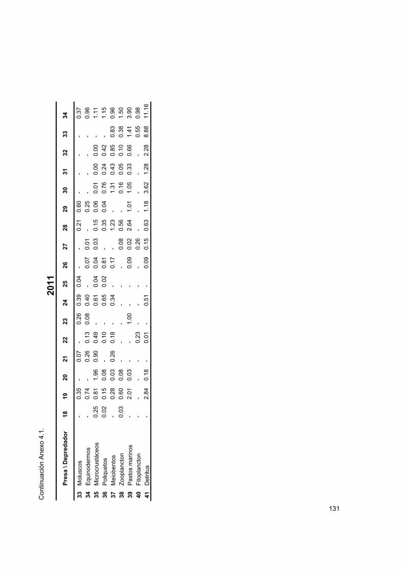
C
ont
inu
ació
n A
nexo
4.1
.
2011
P
resa
\ D
epre
dad
or
18
19
20
21
22
23
24
25
26
27
28
29
30
31
32
33
34
33
Mol
usco
s -
0.35
-
0.07
-
0.26
0.
39
0.04
-
- 0.
21
0.60
-
- -
- 0.
37
34
Equ
inod
erm
os
- 0.
74
- 0.
26
0.13
0.
08
0.40
-
0.07
0.
01
- 0.
25
- -
- -
0.96
35
Mic
rocr
ustá
ceo
s 0.
25
0.81
1.
96
0.90
0.
49
- 0.
61
0.04
0.
04
0.03
0.
15
0.06
0.
01
0.00
0.
00
- 1.
11
36
Pol
ique
tos
0.02
0.
15
0.08
-
0.10
-
0.65
0.
02
0.81
-
0.35
0.
04
0.76
0.
24
0.42
-
1.15
37
Mei
obe
ntos
-
0.28
0.
03
0.26
0.
18
- 0.
34
- 0.
17
- 1.
23
- 1.
31
0.43
0.
85
0.83
0.
96
38
Zoo
plan
cton
0.
03
0.60
0.
08
- -
- -
- -
0.08
0.
56
- 0.
16
0.05
0.
10
0.38
1.
50
39
Pas
tos
mar
inos
-
2.01
0.
03
- -
1.00
-
- 0.
09
0.02
2.
64
1.01
1.
05
0.33
0.
66
1.41
3.
90
40
Fito
plan
cton
-
- -
- 0.
23
- -
- -
0.26
-
- -
- -
0.55
0.
98
41
Det
ritus
-
2.84
0.
18
- 0.
01
- 0.
51
- 0.
09
0.15
0.
63
1.18
3.
62
1.28
2.
28
8.88
11
.16
131

C
ont
inu
ació
n A
nexo
4.1
.
2011
P
res
a \
De
pre
dad
or
35
36
3
7
38
39
40
4
1
1 D
elfin
es
- -
- -
- -
0.17
2 A
ves
Mar
inas
-
- -
- -
- 0.
40
3 T
ortu
gas
Mar
inas
-
- -
- -
- 0.
38
4 A
guja
s -
- -
- -
- 0.
09
5 A
ncho
veta
s -
- -
- -
- 0.
21
6 A
ngu
ilas
- -
- -
- -
0.09
7 B
agre
-
- -
- -
- 0.
42
8 B
arbu
dos
- -
- -
- -
0.18
9 C
intil
las
- -
- -
- -
0.04
10
Cor
vin
as
- -
- -
- -
1.07
11
Igua
nas
- -
- -
- -
0.08
12
Isab
elita
s -
- -
- -
- 0.
16
13
Jure
les
- -
- -
- -
0.15
14
Lisa
s -
- -
- -
- 0.
06
15
Mer
os
- -
- -
- -
0.02
16
Moj
arra
s -
- -
- -
- 1.
18
17
Moj
arra
s m
exic
anas
-
- -
- -
- 0.
01
18
Par
gos
- -
- -
- -
0.17
19
Pec
es g
lobo
-
- -
- -
- 1.
82
20
Pec
es p
lano
s -
- -
- -
- 0.
54
21
Pec
es R
oca
- -
- -
- -
0.67
22
Pej
esap
os
- -
- -
- -
0.37
23
Per
icos
-
- -
- -
- 0.
35
24
Ray
as
- -
- -
- -
0.90
25
Rob
alos
-
- -
- -
- 0.
08
26
Ron
cos
- -
- -
- -
0.44
27
Sar
dina
s -
- -
- -
- 0.
12
28
Sar
gos
- -
- -
- -
1.42
29
Jaib
as
- -
- -
- -
0.83
30
Cam
aró
n bl
anco
-
- -
- -
- 1.
67
31
Cam
aró
n ca
fé
- -
- -
- -
0.62
32
Cam
aró
n ro
sado
-
- -
- -
- 1.
07
Co
ntin
uac
ión
Ane
xo 4
.1.
132

2011
P
res
a \
De
pre
dad
or
35
36
3
7
38
39
40
4
1
33
Mol
usco
s -
- -
- -
- 3.
06
34
Equ
inod
erm
os
- -
- -
- -
4.94
35
Mic
rocr
ustá
ceo
s 0.
76
- -
- -
- 8.
06
36
Pol
ique
tos
- -
2.13
-
- -
22.3
4
37
Mei
obe
ntos
2.
72
5.09
2.
10
- -
- 22
.45
38
Zoo
plan
cton
-
- 0.
10
0.74
-
- 4.
83
39
Pas
tos
mar
inos
14
.34
2.
24
2.13
-
- -
685.
40
40
Fito
plan
cton
-
- -
17
.93
-
- 11
9.0
4
41
Det
ritus
18
.79
70
.33
89
.48
2.
99
- -
-
133

134
Anexo 4.2. Parámetros de entrada en el modelo, indicadores estimados e índice de diversidad funcional para cada uno de los grupos funcionales en los modelos de la Laguna de Términos para los tres periodos (1980, 1998 y 2011) (Abascal-Monroy et al., 2015).
Grupo funcional - 1980 B
(t/km²) P/B
(año-1) Q/B
(año-1) P/Q
R (t/km²/año)
TL P/R
Delfines 0.025 0.100 33.500 0.003 0.668 3.697 0.004Aves Marinas 0.025 0.100 75.000 0.001 1.498 3.924 0.002Tortugas Marinas 0.524 0.150 3.500 0.043 1.388 2.644 0.057Agujas 0.017 2.026 15.835 0.128 0.185 3.064 0.190Anchovetas 0.018 3.356 16.782 0.200 0.180 2.870 0.333Anguilas 0.052 0.510 7.712 0.066 0.297 3.304 0.090Bagres 0.514 1.190 6.468 0.184 2.048 2.529 0.299Barbudos 0.098 3.093 15.736 0.197 0.926 3.242 0.326Cintillas 0.009 0.824 5.752 0.143 0.034 3.676 0.218Corvinas 0.437 0.720 12.511 0.058 4.059 3.322 0.078Iguanas 0.025 1.490 9.750 0.153 0.158 3.276 0.236Isabelitas 0.098 0.615 18.703 0.033 1.410 3.081 0.043Jureles 0.036 1.224 13.283 0.092 0.335 3.191 0.130Lisas 0.329 1.785 19.130 0.093 1.825 2.555 0.132Meros 0.088 2.451 10.632 0.231 0.133 3.471 0.405Mojarras 0.237 1.900 13.461 0.141 2.102 2.925 0.214Mojarras Mexicanas 0.074 1.410 10.895 0.129 0.538 2.843 0.193Pargos 0.118 0.690 7.421 0.093 0.619 3.343 0.132Peces Globo 0.624 1.195 15.080 0.079 6.782 2.438 0.110Peces Planos 0.106 1.502 13.248 0.113 0.964 3.009 0.165Peces Roca 0.187 1.355 7.970 0.170 0.939 3.256 0.270Pejesapos 0.071 1.126 9.323 0.121 0.452 3.117 0.178Pericos 0.121 1.260 36.000 0.035 1.033 2.425 0.046Rayas 0.705 0.558 6.781 0.082 3.431 2.989 0.115Robálos 0.029 1.420 5.389 0.263 0.084 3.373 0.491Roncos 0.130 0.870 7.758 0.112 0.694 3.153 0.163Sardinas 0.025 1.413 11.938 0.118 0.206 2.298 0.174Sargos 0.753 2.230 19.568 0.114 10.109 2.480 0.166Jaibas 0.180 2.358 6.285 0.375 0.481 2.424 0.883Camarón Blanco 0.245 13.500 35.500 0.380 3.651 2.376 0.906Camarón Café 0.124 12.000 34.300 0.350 1.915 2.378 0.777Camarón Rosado 0.203 12.500 35.700 0.350 3.260 2.378 0.778Moluscos 1.506 4.623 15.765 0.293 12.031 2.106 0.579Equinodermos 4.569 2.245 12.596 0.178 35.783 2.324 0.287Microcrustáceos 1.802 11.443 35.795 0.320 30.982 2.099 0.666Poliquetos 8.013 4.425 21.544 0.205 102.648 2.065 0.345Meiobentos 4.182 10.383 48.763 0.213 119.720 2.043 0.363Zooplancton 1.127 18.624 71.974 0.259 43.903 2.033 0.478Pastos Marinos 178.637 8.821 0.000 -- 0.000 1.000 --Fitoplancton 149.033 3.674 0.000 -- 0.000 1.000 --
Detritos 84.710 -- -- -- 0.000 1.000 --
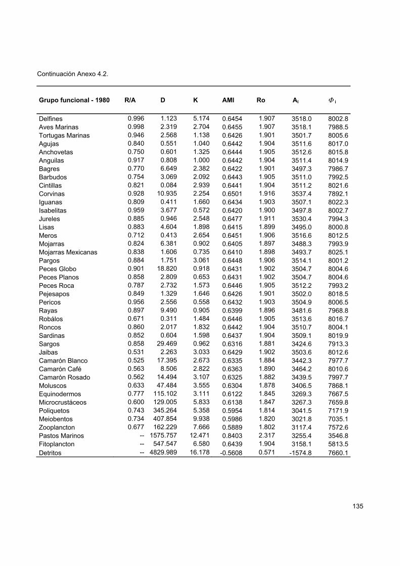
135
Continuación Anexo 4.2.
Grupo funcional - 1980 R/A D K AMI Ro Ai Φ i
Delfines 0.996 1.123 5.174 0.6454 1.907 3518.0 8002.8Aves Marinas 0.998 2.319 2.704 0.6455 1.907 3518.1 7988.5Tortugas Marinas 0.946 2.568 1.138 0.6426 1.901 3501.7 8005.6Agujas 0.840 0.551 1.040 0.6442 1.904 3511.6 8017.0Anchovetas 0.750 0.601 1.325 0.6444 1.905 3512.6 8015.8Anguilas 0.917 0.808 1.000 0.6442 1.904 3511.4 8014.9Bagres 0.770 6.649 2.382 0.6422 1.901 3497.3 7986.7Barbudos 0.754 3.069 2.092 0.6443 1.905 3511.0 7992.5Cintillas 0.821 0.084 2.939 0.6441 1.904 3511.2 8021.6Corvinas 0.928 10.935 2.254 0.6501 1.916 3537.4 7892.1Iguanas 0.809 0.411 1.660 0.6434 1.903 3507.1 8022.3Isabelitas 0.959 3.677 0.572 0.6420 1.900 3497.8 8002.7Jureles 0.885 0.946 2.548 0.6477 1.911 3530.4 7994.3Lisas 0.883 4.604 1.898 0.6415 1.899 3495.0 8000.8Meros 0.712 0.413 2.654 0.6451 1.906 3516.6 8012.5Mojarras 0.824 6.381 0.902 0.6405 1.897 3488.3 7993.9Mojarras Mexicanas 0.838 1.606 0.735 0.6410 1.898 3493.7 8025.1Pargos 0.884 1.751 3.061 0.6448 1.906 3514.1 8001.2Peces Globo 0.901 18.820 0.918 0.6431 1.902 3504.7 8004.6Peces Planos 0.858 2.809 0.653 0.6431 1.902 3504.7 8004.6Peces Roca 0.787 2.732 1.573 0.6446 1.905 3512.2 7993.2Pejesapos 0.849 1.329 1.646 0.6426 1.901 3502.0 8018.5Pericos 0.956 2.556 0.558 0.6432 1.903 3504.9 8006.5Rayas 0.897 9.490 0.905 0.6399 1.896 3481.6 7968.8Robálos 0.671 0.311 1.484 0.6446 1.905 3513.6 8016.7Roncos 0.860 2.017 1.832 0.6442 1.904 3510.7 8004.1Sardinas 0.852 0.604 1.598 0.6437 1.904 3509.1 8019.9Sargos 0.858 29.469 0.962 0.6316 1.881 3424.6 7913.3Jaibas 0.531 2.263 3.033 0.6429 1.902 3503.6 8012.6Camarón Blanco 0.525 17.395 2.673 0.6335 1.884 3442.3 7977.7Camarón Café 0.563 8.506 2.822 0.6363 1.890 3464.2 8010.6Camarón Rosado 0.562 14.494 3.107 0.6325 1.882 3439.5 7997.7Moluscos 0.633 47.484 3.555 0.6304 1.878 3406.5 7868.1Equinodermos 0.777 115.102 3.111 0.6122 1.845 3269.3 7667.5Microcrustáceos 0.600 129.005 5.833 0.6138 1.847 3267.3 7659.8Poliquetos 0.743 345.264 5.358 0.5954 1.814 3041.5 7171.9Meiobentos 0.734 407.854 9.938 0.5986 1.820 3021.8 7035.1Zooplancton 0.677 162.229 7.666 0.5889 1.802 3117.4 7572.6Pastos Marinos -- 1575.757 12.471 0.8403 2.317 3255.4 3546.8Fitoplancton -- 547.547 6.580 0.6439 1.904 3158.1 5813.5Detritos -- 4829.989 16.178 -0.5608 0.571 -1574.8 7660.1

136
Continuación Anexo 4.2.
Grupo funcional - 1980 Ci (A/C)i Ai/A (O/C)i FADI
Delfines 11520.8 0.305 1.008 0.6946 0.708Aves Marinas 11506.6 0.306 1.008 0.6943 0.708Tortugas Marinas 11507.3 0.304 1.003 0.6957 0.708Agujas 11528.7 0.305 1.006 0.6954 0.701Anchovetas 11528.4 0.305 1.006 0.6953 0.676Anguilas 11526.3 0.305 1.006 0.6954 0.704Bagres 11484.0 0.305 1.002 0.6955 0.450Barbudos 11503.5 0.305 1.006 0.6948 0.702Cintillas 11532.8 0.304 1.006 0.6955 0.703Corvinas 11429.5 0.310 1.013 0.6905 0.599Iguanas 11529.4 0.304 1.005 0.6958 0.701Isabelitas 11500.6 0.304 1.002 0.6959 0.695Jureles 11524.7 0.306 1.011 0.6937 0.699Lisas 11495.8 0.304 1.001 0.6960 0.704Meros 11529.0 0.305 1.007 0.6950 0.704Mojarras 11482.2 0.304 0.999 0.6962 0.638Mojarras Mexicanas 11518.8 0.303 1.001 0.6967 0.702Pargos 11515.3 0.305 1.007 0.6948 0.701Peces Globo 11509.3 0.305 1.004 0.6955 0.576Peces Planos 11509.3 0.305 1.004 0.6955 0.679Peces Roca 11505.4 0.305 1.006 0.6947 0.699Pejesapos 11520.4 0.304 1.003 0.6960 0.703Pericos 11511.4 0.304 1.004 0.6955 0.704Rayas 11450.3 0.304 0.997 0.6959 0.702Robálos 11530.4 0.305 1.007 0.6953 0.704Roncos 11514.8 0.305 1.006 0.6951 0.696Sardinas 11529.0 0.304 1.005 0.6956 0.701Sargos 11337.9 0.302 0.981 0.6980 0.650Jaibas 11516.1 0.304 1.004 0.6958 0.708Camarón Blanco 11420.0 0.301 0.986 0.6986 0.708Camarón Café 11474.8 0.302 0.992 0.6981 0.708Camarón Rosado 11437.3 0.301 0.985 0.6993 0.708Moluscos 11274.5 0.302 0.976 0.6979 0.708Equinodermos 10936.8 0.299 0.937 0.7011 0.708Microcrustáceos 10927.1 0.299 0.936 0.7010 0.708Poliquetos 10213.4 0.298 0.871 0.7022 0.708Meiobentos 10056.9 0.300 0.866 0.6995 0.708
Zooplancton 10690.0 0.292 0.893 0.7084 0.708
Pastos Marinos 6802.2 0.479 0.933 0.5214 0.708Fitoplancton 8971.6 0.352 0.905 0.6480 0.708
Detritos 6085.2 -0.259 -0.451 1.2588 0.708

137
Continuación Anexo 4.2.
Grupo funcional - 1998 B
(t/km²) P/B
(año-1) Q/B
(año-1) P/Q
R (t/km²/año)
TL P/R
Delfines 0.0250 0.100 33.50 0.0030 0.668 3.608 0.0037Aves Marinas 0.0250 0.100 75.00 0.0013 1.498 3.896 0.0017Tortugas Marinas 0.5238 0.150 3.50 0.0429 1.388 2.630 0.0566Agujas 0.0520 1.985 14.20 0.1398 0.488 3.062 0.2117Anchovetas 0.0620 3.225 17.00 0.1897 0.643 2.870 0.3108Anguilas 0.1480 0.510 7.72 0.0661 0.838 3.328 0.0901Bagres 0.3920 1.085 6.20 0.1750 1.519 2.499 0.2800Barbudos 0.0320 3.320 17.20 0.1930 0.334 3.254 0.3180Cintillas 0.0220 1.555 8.00 0.1944 0.107 3.755 0.3209Corvinas 0.2640 1.949 14.33 0.1360 2.512 3.243 0.2048Iguanas 0.2640 1.415 9.75 0.1451 1.686 3.063 0.2216Isabelitas 0.1110 0.690 19.50 0.0354 1.655 3.081 0.0463Jureles 0.0790 1.150 14.31 0.0804 0.814 3.080 0.1117Lisas 0.0197 1.888 20.80 0.0908 0.290 2.555 0.1280Meros 0.1030 2.285 12.24 0.1867 0.773 3.425 0.3044Mojarras 0.4390 1.693 17.02 0.0995 5.234 2.930 0.1420Mojarras Mexicanas 0.0360 1.280 7.10 0.1803 0.158 2.856 0.2909Pargos 0.1970 0.969 7.00 0.1384 0.912 3.316 0.2092Peces Globo 0.4210 1.100 14.80 0.0743 4.522 2.438 0.1024Peces Planos 0.0540 0.920 15.00 0.0613 0.598 3.009 0.0830Peces Roca 0.0430 1.345 7.97 0.1688 0.216 3.252 0.2673Pejesapos 0.0870 1.600 13.40 0.1194 0.793 3.030 0.1754Pericos 0.0343 1.260 36.00 0.0350 0.943 2.516 0.0458Rayas 2.2620 0.620 5.18 0.1197 7.971 2.989 0.1759Robálos 0.1310 1.000 6.60 0.1515 0.561 3.333 0.2336Roncos 0.0860 0.855 12.50 0.0684 0.786 3.143 0.0935Sardinas 0.0510 1.400 13.60 0.1029 0.483 2.281 0.1477Sargos 0.3000 2.591 21.40 0.1211 4.359 2.481 0.1783Jaibas 1.0435 2.230 6.29 0.3545 2.924 2.420 0.7959Camarón Blanco 0.2613 13.500 35.50 0.3803 3.893 2.376 0.9060Camarón Café 0.0852 12.500 35.70 0.3501 1.368 2.378 0.7783Camarón Rosado 0.1243 12.000 34.30 0.3499 1.920 2.378 0.7772Moluscos 1.2981 4.620 15.77 0.2930 10.379 2.106 0.5778Equinodermos 3.1333 2.250 12.60 0.1786 24.534 2.324 0.2874Microcrustáceos 1.1841 11.440 35.80 0.3196 20.367 2.099 0.6651Poliquetos 7.1050 4.430 21.54 0.2057 90.958 2.065 0.3460Meiobentos 2.7640 10.380 48.76 0.2129 79.128 2.043 0.3626Zooplancton 0.4474 18.620 71.97 0.2587 17.427 2.033 0.4780Pastos Marinos 99.0843 8.820 0.00 -- 0.000 1.000 --Fitoplancton 58.4804 3.670 0.00 -- 0.000 1.000 --
Detritos 84.7100 -- -- -- 0.000 1.000 --

138
Continuación Anexo 4.2.
Grupo funcional - 1998 R/A D K AMI Ro Ai Φ i
Delfines 0.9963 1.0717 4.477 0.7343 2.0841 2256.6 4646.0Aves Marinas 0.9983 2.1632 2.724 0.7342 2.0838 2255.5 4634.9Tortugas Marinas 0.9464 2.5594 1.15 0.7318 2.0789 2247.4 4642.1Agujas 0.8253 1.4768 1.045 0.7332 2.0818 2252.4 4648.2Anchovetas 0.7629 2.1080 1.281 0.7327 2.0808 2251.0 4645.3Anguilas 0.9174 2.2839 1.006 0.7325 2.0803 2250.3 4644.1Bagres 0.7812 4.8608 2.402 0.7321 2.0794 2246.7 4632.2Barbudos 0.7587 1.1008 2.119 0.7297 2.0745 2241.6 4661.4Cintillas 0.7570 0.3308 2.893 0.7321 2.0794 2250.4 4661.9Corvinas 0.8300 7.5662 2.267 0.7341 2.0836 2250.8 4593.5Iguanas 0.8186 4.8351 1.668 0.7320 2.0793 2245.9 4625.3Isabelitas 0.9558 4.3290 0.573 0.7302 2.0755 2241.8 4637.2Jureles 0.8995 2.2610 2.612 0.7321 2.0794 2249.0 4645.5Lisas 0.8865 0.7299 1.905 0.7342 2.0837 2256.1 4652.3Meros 0.7666 2.2892 2.669 0.7339 2.0832 2253.9 4636.3Mojarras 0.8757 14.9436 0.913 0.7220 2.0586 2208.7 4599.6Mojarras Mexicanas 0.7746 0.5112 0.743 0.7336 2.0826 2254.3 4655.6Pargos 0.8270 2.7580 3.067 0.7336 2.0826 2253.6 4635.5Peces Globo 0.9071 12.4616 0.93 0.7310 2.0772 2247.1 4668.8Peces Planos 0.9233 1.6200 0.654 0.7318 2.0788 2248.0 4651.9Peces Roca 0.7891 0.6282 1.582 0.7344 2.0842 2256.8 4651.5Pejesapos 0.8507 2.3316 1.663 0.7297 2.0744 2241.6 4652.9Pericos 0.9563 2.4454 0.569 0.7315 2.0781 2247.1 4648.6Rayas 0.8504 23.3054 0.916 0.7164 2.0471 2185.0 4555.3Robálos 0.8106 1.7292 1.496 0.7298 2.0746 2241.8 4655.3Roncos 0.9145 2.1500 1.848 0.7332 2.0817 2252.3 4643.4Sardinas 0.8713 1.3872 1.605 0.7337 2.0829 2254.1 4648.9Sargos 0.8487 12.8400 0.969 0.7263 2.0674 2223.1 4604.9Jaibas 0.5568 13.1274 3.038 0.7226 2.0599 2212.7 4614.7Camarón Blanco 0.5246 18.5507 2.674 0.7234 2.0614 2210.0 4592.5Camarón Café 0.5623 6.0840 2.823 0.7306 2.0764 2240.1 4630.6Camarón Rosado 0.5627 8.5289 3.108 0.7297 2.0744 2236.4 4621.4Moluscos 0.6338 40.9416 3.562 0.7198 2.0540 2183.8 4521.1Equinodermos 0.7768 78.9592 3.066 0.6997 2.0131 2096.9 4419.3Microcrustáceos 0.6006 84.7817 5.837 0.7070 2.0280 2114.8 4413.5Poliquetos 0.7429 306.0818 5.362 0.6781 1.9702 1879.1 3972.8Meiobentos 0.7339 269.5465 9.94 0.7088 2.0316 1989.7 3981.5Zooplancton 0.6766 64.3924 7.663 0.6929 1.9996 2088.5 4464.9Pastos Marinos -- 873.9235 12.471 0.9216 2.5132 2032.0 2242.0Fitoplancton -- 214.6230 6.57 0.7164 2.0470 2049.5 3745.6Detritos -- 2619.5014 16.184 -0.3268 0.7212 -521.9 4370.1

139
Continuación Anexo 4.2.
Grupo funcional - 1998 Ci (A/C)i Ai/A (O/C)i FADI
Delfines 6902.6 0.3269 1.0042 0.6731 0.716Aves Marinas 6890.4 0.3273 1.0037 0.6727 0.716Tortugas Marinas 6889.5 0.3262 1.0001 0.6738 0.716Agujas 6900.6 0.3264 1.0024 0.6736 0.697Anchovetas 6896.3 0.3264 1.0017 0.6736 0.667
Anguilas 6894.4 0.3264 1.0014 0.6736 0.697
Bagres 6878.9 0.3266 0.9998 0.6734 0.439
Barbudos 6903.0 0.3247 0.9976 0.6753 0.697
Cintillas 6912.3 0.3256 1.0015 0.6744 0.695Corvinas 6844.3 0.3289 1.0016 0.6711 0.626Iguanas 6871.2 0.3269 0.9995 0.6731 0.694
Isabelitas 6879.0 0.3259 0.9976 0.6741 0.690
Jureles 6894.5 0.3262 1.0008 0.6738 0.679
Lisas 6908.3 0.3266 1.0040 0.6734 0.697
Meros 6890.1 0.3271 1.0030 0.6729 0.697Mojarras 6808.4 0.3244 0.9829 0.6756 0.479Mojarras Mexicanas 6910.0 0.3262 1.0032 0.6738 0.697
Pargos 6889.1 0.3271 1.0029 0.6729 0.690
Peces Globo 6915.9 0.3249 1.0000 0.6751 0.673
Peces Planos 6899.9 0.3258 1.0004 0.6742 0.688
Peces Roca 6908.3 0.3267 1.0043 0.6733 0.696Pejesapos 6894.5 0.3251 0.9976 0.6749 0.697Pericos 6895.7 0.3259 1.0000 0.6741 0.697Rayas 6740.4 0.3242 0.9724 0.6758 0.695
Robálos 6897.1 0.3250 0.9976 0.6750 0.696
Roncos 6895.7 0.3266 1.0023 0.6734 0.694
Sardinas 6903.0 0.3265 1.0031 0.6735 0.693
Sargos 6828.0 0.3256 0.9893 0.6744 0.668Jaibas 6827.5 0.3241 0.9847 0.6759 0.716Camarón Blanco 6802.5 0.3249 0.9835 0.6751 0.716Camarón Café 6870.7 0.3260 0.9969 0.6740 0.716Camarón Rosado 6857.8 0.3261 0.9953 0.6739 0.716Moluscos 6704.9 0.3257 0.9718 0.6743 0.716Equinodermos 6516.3 0.3218 0.9332 0.6782 0.716Microcrustáceos 6528.3 0.3239 0.9411 0.6761 0.716Poliquetos 5851.8 0.3211 0.8362 0.6789 0.716Meiobentos 5971.2 0.3332 0.8855 0.6668 0.716Zooplancton 6553.4 0.3187 0.9294 0.6813 0.716Pastos Marinos 4274.0 0.4754 0.9043 0.5246 0.716Fitoplancton 5795.1 0.3537 0.9121 0.6463 0.716
Detritos 3848.3 -0.1356 -0.2322 1.1356 0.716

140
Continuación Anexo 4.2.
Grupo funcional - 2011 B
(t/km²) P/B
(año-1) Q/B
(año-1) P/Q
R (t/km²/año)
TL P/R
Delfines 0.025 0.100 33.50 0.0030 0.6675 3.571 0.0037Aves Marinas 0.025 0.100 75.00 0.0013 1.4975 4.027 0.0017Tortugas Marinas 0.524 0.150 3.50 0.0429 1.3881 2.634 0.0566Agujas 0.021 1.967 14.20 0.1385 0.1973 3.062 0.2094Anchovetas 0.041 3.175 17.00 0.1868 0.4274 2.870 0.3046Anguilas 0.057 0.513 7.72 0.0665 0.3226 3.322 0.0906Bagres 0.205 1.070 6.20 0.1726 0.7974 2.499 0.2751Barbudos 0.032 3.320 17.20 0.1930 0.3341 3.226 0.3180Cintillas 0.019 1.175 8.00 0.1469 0.0993 3.707 0.2249Corvinas 0.398 1.205 14.33 0.0841 4.0831 3.203 0.1175Iguanas 0.035 1.376 9.75 0.1411 0.2248 3.044 0.2142Isabelitas 0.035 0.690 19.50 0.0354 0.5219 3.081 0.0463Jureles 0.039 1.150 14.31 0.0804 0.4016 3.035 0.1117Lisas 0.011 1.882 20.80 0.0905 0.1694 2.555 0.1275Meros 0.009 2.365 12.24 0.1932 0.0668 3.416 0.3184Mojarras 0.225 1.647 17.02 0.0968 2.6930 2.930 0.1376Mojarras Mexicanas 0.009 1.150 7.10 0.1620 0.0408 2.855 0.2539Pargos 0.098 1.408 7.50 0.1877 0.4500 3.314 0.3066Peces Globo 0.551 1.060 14.80 0.0716 5.9398 2.438 0.0983Peces Planos 0.155 0.910 15.00 0.0607 1.7190 3.009 0.0821Peces Roca 0.422 1.330 7.97 0.1669 2.1294 3.251 0.2636Pejesapos 0.093 1.600 13.40 0.1194 0.8482 3.000 0.1754Pericos 0.052 1.260 36.00 0.0350 1.4333 2.514 0.0458Rayas 0.612 0.548 5.18 0.1058 2.2008 2.988 0.1524Robálos 0.037 1.000 6.60 0.1515 0.1584 3.319 0.2336Roncos 0.117 0.805 12.50 0.0644 1.0758 3.117 0.0875Sardinas 0.046 1.386 13.60 0.1019 0.4367 2.274 0.1460Sargos 0.272 2.590 21.40 0.1210 3.9522 2.476 0.1783Jaibas 0.634 2.230 6.29 0.3545 1.7765 2.412 0.7959Camarón Blanco 0.238 13.500 35.50 0.3803 3.5452 2.376 0.9060Camarón Café 0.078 12.500 35.70 0.3501 1.2546 2.378 0.7783Camarón Rosado 0.131 12.000 34.30 0.3499 2.0294 2.378 0.7772Moluscos 0.668 4.620 15.77 0.2930 5.3374 2.106 0.5778Equinodermos 1.861 2.250 12.60 0.1786 14.5688 2.324 0.2874Microcrustáceos 1.041 11.440 35.80 0.3196 17.9055 2.099 0.6651Poliquetos 4.388 4.430 21.54 0.2057 56.1740 2.065 0.3460Meiobentos 1.999 10.380 48.76 0.2129 57.2371 2.043 0.3626Zooplancton 0.300 18.620 71.97 0.2587 11.6679 2.033 0.4780Pastos Marinos 77.632 8.820 0.00 -- 0.0000 1.000 --Fitoplancton 38.849 3.670 0.00 -- 0.0000 1.000 --
Detritos 84.710 -- -- -- 0.0000 1.000 --

141
Continuación Anexo 4.2.
Grupo funcional - 2011 R/A D K AMI Ro Ai Φ i
Delfines 0.9963 0.9657 3.226 0.7132 2.0406 1633.3 3322.6Aves Marinas 0.9983 2.1962 5.54 0.7139 2.0420 1634.2 3308.7Tortugas Marinas 0.9464 2.3506 5.682 0.7109 2.0359 1627.3 3317.9Agujas 0.8268 0.5715 2.71 0.7096 2.0333 1625.8 3337.0Anchovetas 0.7665 1.4333 1.147 0.7096 2.0331 1624.9 3330.1Anguilas 0.9169 0.8992 4.459 0.7129 2.0399 1633.3 3326.7Bagres 0.7843 2.7271 2.882 0.7078 2.0295 1619.4 3326.8Barbudos 0.7587 1.1626 1.487 0.7088 2.0316 1623.3 3333.0Cintillas 0.8164 0.2969 2.604 0.7130 2.0402 1633.6 3331.1Corvinas 0.8949 9.1920 0.736 0.7105 2.0350 1621.3 3266.6Iguanas 0.8236 0.7025 2.11 0.7133 2.0407 1634.1 3327.6Isabelitas 0.9558 1.6162 1.006 0.7112 2.0364 1627.9 3324.5Jureles 0.8995 1.0576 0.572 0.7108 2.0356 1627.8 3329.8Lisas 0.8869 0.4726 0.566 0.7139 2.0419 1635.5 3328.4Meros 0.7585 0.1970 0.654 0.7135 2.0411 1634.6 3331.1Mojarras 0.8790 8.7302 0.913 0.7033 2.0204 1605.6 3297.6Mojarras Mexicanas 0.7975 0.1273 1.656 0.7129 2.0400 1633.3 3333.3Pargos 0.7653 1.3485 1.577 0.7115 2.0370 1629.3 3325.1Peces Globo 0.9105 15.5944 1.845 0.6995 2.0127 1591.3 3275.9Peces Planos 0.9242 4.8203 2.665 0.7068 2.0275 1615.7 3311.1Peces Roca 0.7914 5.7286 1.659 0.7082 2.0303 1618.2 3296.4Pejesapos 0.8507 2.5880 0.929 0.7090 2.0320 1622.9 3322.5Pericos 0.9563 3.2749 0.968 0.7089 2.0318 1622.1 3319.7Rayas 0.8678 6.7136 0.91 0.7059 2.0256 1612.9 3300.9Robálos 0.8106 0.5417 2.257 0.7106 2.0353 1628.1 3334.5Roncos 0.9195 3.7334 3.063 0.7096 2.0331 1622.8 3311.8Sardinas 0.8726 1.0916 2.397 0.7125 2.0390 1631.5 3327.1Sargos 0.8487 11.5725 1.045 0.7028 2.0195 1601.8 3288.4Jaibas 0.5568 6.5310 1.333 0.7043 2.0224 1608.6 3312.3Camarón Blanco 0.5246 14.2835 1.603 0.6994 2.0126 1591.2 3287.4Camarón Café 0.5623 4.7982 1.902 0.7087 2.0314 1620.1 3314.3Camarón Rosado 0.5627 8.9213 12.474 0.7066 2.0272 1613.2 3298.1Moluscos 0.6338 24.1121 16.183 0.7001 2.0140 1587.1 3252.0Equinodermos 0.7768 44.3689 2.671 0.6849 1.9836 1538.9 3195.5Microcrustáceos 0.6006 73.2080 2.819 0.6780 1.9700 1503.2 3136.1Poliquetos 0.7429 155.3262 3.039 0.6683 1.9510 1428.3 2953.2Meiobentos 0.7339 191.8575 3.063 0.6761 1.9663 1421.2 2867.3Zooplancton 0.6766 43.3183 3.104 0.6745 1.9630 1516.2 3197.4Pastos Marinos -- 719.0987 3.563 0.9037 2.4687 1419.7 1490.3Fitoplancton -- 139.1873 5.357 0.6890 1.9918 1482.8 2728.3Detritos -- 1987.5459 5.839 -0.3987 0.6712 -474.1 3152.6

142
Continuación Anexo 4.2.
Grupo funcional - 2011 Ci (A/C)i Ai/A (O/C)i
FADI
Delfines 4956.0 0.3296 1.0043 0.6704 0.690Aves Marinas 4942.9 0.3306 1.0049 0.6694 0.690Tortugas Marinas 4945.2 0.3291 1.0006 0.6709 0.690Agujas 4962.8 0.3276 0.9997 0.6724 0.676Anchovetas 4955.0 0.3279 0.9992 0.6721 0.665
Anguilas 4960.0 0.3293 1.0043 0.6707 0.677
Bagres 4946.2 0.3274 0.9958 0.6726 0.570
Barbudos 4956.3 0.3275 0.9982 0.6725 0.676
Cintillas 4964.7 0.3290 1.0045 0.6710 0.675Corvinas 4887.9 0.3317 0.9970 0.6683 0.616Iguanas 4961.7 0.3293 1.0048 0.6707 0.670
Isabelitas 4952.3 0.3287 1.0010 0.6713 0.662
Jureles 4957.5 0.3283 1.0009 0.6717 0.668
Lisas 4963.9 0.3295 1.0057 0.6705 0.677
Meros 4965.7 0.3292 1.0051 0.6708 0.677Mojarras 4903.2 0.3275 0.9873 0.6725 0.459Mojarras Mexicanas 4966.7 0.3289 1.0044 0.6711 0.677
Pargos 4954.4 0.3288 1.0018 0.6712 0.674
Peces Globo 4867.2 0.3269 0.9785 0.6731 0.625
Peces Planos 4926.8 0.3279 0.9935 0.6721 0.624
Peces Roca 4914.6 0.3293 0.9951 0.6707 0.646Pejesapos 4945.4 0.3282 0.9979 0.6718 0.677Pericos 4941.8 0.3282 0.9974 0.6718 0.677Rayas 4913.8 0.3282 0.9918 0.6718 0.669
Robálos 4962.6 0.3281 1.0011 0.6719 0.677
Roncos 4934.6 0.3289 0.9979 0.6711 0.666
Sardinas 4958.6 0.3290 1.0033 0.6710 0.665
Sargos 4890.2 0.3275 0.9849 0.6725 0.610Jaibas 4920.8 0.3269 0.9891 0.6731 0.690Camarón Blanco 4878.7 0.3262 0.9785 0.6738 0.690Camarón Café 4934.5 0.3283 0.9962 0.6717 0.690Camarón Rosado 4911.3 0.3285 0.9920 0.6715 0.690Moluscos 4839.2 0.3280 0.9760 0.6720 0.690Equinodermos 4734.4 0.3251 0.9463 0.6749 0.690Microcrustáceos 4639.3 0.3240 0.9243 0.6760 0.690Poliquetos 4381.4 0.3260 0.8783 0.6740 0.690Meiobentos 4288.5 0.3314 0.8739 0.6686 0.690Zooplancton 4713.6 0.3217 0.9323 0.6783 0.690Pastos Marinos 2910.0 0.4879 0.8730 0.5121 0.690Fitoplancton 4211.1 0.3521 0.9118 0.6479 0.690
Detritos 2678.5 -0.1770 -0.2915 1.1770 0.690

Proceedings of the 65th Gulf and Caribbean Fisheries Institute November 5 – 9, 2012 Santa Marta, Colombia
Incidencia de la Pesca Artesanal Sobre la Diversidad Taxonómica y Funcional de la
Comunidad de Peces en el Mar Caribe de Colombia
Artisanal Fisheries Incidence on Taxonomic and Functional Diversity of the Fish
Community in the Caribbean Sea off Colombia
L'Impact de la Pêche sur la Diversité Taxonomique et Fonctionnelle de la Communauté de
Poissons dans la Mer des Caraïbes de la Colombie
FABIÁN D. ESCOBAR-TOLEDO1,2*, MARÍA DEL PILAR PARRADO-CORTÉS2,
LUIS ORLANDO DUARTE2, y MANUEL ZETINA-REJÓN1 1Centro Interdisciplinario de Ciencias Marinas, Instituto Politécnico Nacional, P.O. Box 592,
La Paz, 23096 Baja California Sur, México. 2Laboratorio de Investigaciones Pesqueras Tropicales, Universidad del
Magdalena, Carrera 32 # 22-08, Santa Marta, Colombia. *[email protected].
RESUMEN A nivel mundial, en especial en Latinoamérica, la pesca artesanal genera altos niveles de captura y es una de las principales
actividades productivas de las zonas costeras tropicales. Sin embargo, la fuerte presión generada por esta actividad puede atentar contra la sustentabilidad de los recursos pesqueros limitando el normal desarrollo de los procesos en el ecosistema. Aproximaciones
que evidencien la incidencia de la flota sobre la diversidad taxonómica y funcional de la comunidad de peces aún no se han realizado
en mar Caribe de Colombia. Se pretende, entonces, determinar la incidencia de la pesca artesanal en tres ecoregiones del área de estudio (Golfo de Salamanca, Tayrona, Palomino) entre 1994 y 1998 y en los años 2000 y 2008. Se registraron las capturas diarias
realizadas con los arte de pesca de palangre, red de enmalle y red de tiro en la zona. El análisis se realizó con las capturas
estandarizadas (kg/faena). La diversidad taxonómica y funcional se analizó a través del índice de distinción taxonómica y funcional respectivamente. Se registraron 195 especies para el área durante los años de muestreo. La relación de los índices respecto a los años
no fue significativa. No obstante, el índice de distinción taxonómica presentó una tendencia a disminuir (r = -0.69; p = 0.1291),
mientras que el índice de distinción funcional mostró una tendencia al aumento (r = 0.77; p = 0.0686) a lo largo del tiempo. Asimismo, fue evidente el aumento en el índice de distinción taxonómica a lo largo de un gradiente norte-sur. El análisis de la
distinción funcional permitió identificar a la ecoregión Palomino como la de mayor semejanza funcional en las capturas entre años.
PALABRAS CLAVE: Diversidad taxonómica, diversidad funcional, pescar artesanal, mar Caribe, Colombia
INTRODUCCIÓN
La pesca artesanal genera más de la mitad de la producción mundial pesquera (Agüero y Claverí 2007). Asimismo,
produce más de la tercera parte de la captura que es destinada al consumo humano(Berkes et al. 2001). En el Caribe de
Colombia, esta pesquería ha llegado a producir más de la mitad de la captura total anual generando hasta 4 mil empleos
directos e indirectos en la zona (Barros y Manjarrés 2004) y en los últimos años ha venido experimentando cambios tanto en
la composición de especies como en el volumen de desembarcos (Pardo 2011). Ésta pesquería, que se desarrolla de manera
multiespecífica, está soportada en la explotación de alrededor de 200 especies, entre demersales y pelágicas (Párraga-
Velandia 2009). A pesar de su importancia, los estudios existentes han sido orientados a la caracterización de la flota,
análisis de tendencias y capturas, pero pocas evaluaciones se ha realizado acerca de las implicaciones ecológicas que tienen
la flota sobre las comunidades explotadas.
Así, conocer la diversidad puede ser un punto de partida para la evaluación de posibles efectos de la pesca sobre el
ecosistema (Yáñez-Arancibia y Sánchez-Gil 1988). En este sentido, descriptores ecológicos que se basan en el número de
especies y/o número de individuos (riqueza, dominancia y diversidad) describiendo los cambios en la estructura de la
comunidad han sido los más utilizados (Bevilacqua et al. 2009, Clarke y Warwick 2001a, Magurran 2004). Pero más allá de
estas aproximaciones, se han generado índices que muestran otros aspectos de la estructura ecológica como es la relación
evolutiva entre las especies (Abellán et al. 2006, Ramos-Miranda et al. 2005). Por lo que el uso de este tipo de índices se ha
incrementado con el propósito de brindar herramientas de fácil manejo para la evaluación de la salud de los ecosistemas
acuáticos (Bevilacqua et al. 2011).
En este mismo sentido, algunos autores han utilizado la diversidad como indicador del funcionamiento del ecosistema
(Hooper et al. 2005; Hooper et al. 2002; Tilman et al. 1997), pero su relación con los atributos funcionales no es del todo
evidente (Somerfield et al. 2008). Por consiguiente, se han desarrollado múltiples experimentos donde se manipula la
diversidad tanto de especies como grupos funcionales (Hooper et al. 2002). Sin embargo, cuantificar la diversidad funcional
no ha sido fácil y aún faltan índices que simplifiquen esa complejidad (Hooper et al. 2005; Somerfield et al. 2008). Recien-
temente se ha propuesto un índice que cuantifica algunos aspectos de la estructura de una comunidad considerando atributos
de la historia de vida y características ecológicas de las especies; aunque no es independiente de la diversidad taxonómica,

Escobar-Toledo, F.D. et al. GCFI:65 (2013) Page 347
su utilidad radica en que puede trasmitir otro tipo de
información (Somerfield et al. 2008).
Debido a la continua presión pesquera ejercida por la
pesquería artesanal y a pesar de los conocimientos que se
tienen acerca de la ictiofauna capturada por ésta, no existen
trabajos que evidencien una incidencia sobre la diversidad
taxonómica y funcional del ecosistema para la zona. Por
ello, éste trabajo se enfocó en determinar la variabilidad
espacial y temporal taxonómica y funcional de la comuni-
dad de peces capturados por las pesquerías artesanales en
tres ecoregiones del norte del Mar Caribe de Colombia.
MÉTODOS
El Caribe de Colombia está dividido en dos zonas
naturales (suroeste y noroeste) separadas por la desembo-
cadura del río Magdalena y con características totalmente
diferentes (Andrade-Amaya 2000). Para la zona noroeste,
el Programa Nacional de Investigación en Biodiversidad
Marina y Costera identificó cuatro ecoregiones naturales
marinas y costeras (Diaz-Merlano y Gómez-López 2000).
En este trabajo se contó con registros para la zona com-
prendida entre la desembocadura de los ríos Palomino y
Magdalena (Figura 1), la cual incluye tres de estas
ecoregiones:
i) Palomino (PAL), con amplias playas de grano
grueso, sin la existencia aparente de fanerógamas
y arrecifes de coral, plataforma medianamente
ancha y poca carga de sedimentos que no alteran
la calidad físico-química de las aguas costeras,
ii) Tayrona (TAY), cuyo litoral se alterna entre cabos
rocosos y ensenadas con playas, plataforma casi
ausente, baja influencia de descargas continenta-
les, fondos predominantemente rocosos y
arenosos, y gran diversidad de ambientes
(mosaicos coralinos, fanerógamas, praderas de
algas),
iii) Magdalena (subecoregión Golfo de Salamanca -
GDS), que recibe una marcada influencia de una
laguna costera (Ciénaga Grande de Santa Marta-
CGSM) y del río Magdalena, con aguas predomi-
nantemente turbias, salinidad algo reducida,
plataforma de anchura variable y poco desarrollo
de comunidades ecológicas de sustratos duros,
formaciones coralinas y praderas de fanerógamas.
La pesquería artesanal en esta zona está conformada
por lanchas de fibra de vidrio y/o madera de 4.5 a 9.2 m de
eslora y cuya distribución está determinada por la distancia
a los centros de acopio y las condiciones de navegación,
llegando a operar hasta la isobata de 200 m (Gómez-
Canchong et al. 2004, Párraga-Velandia 2009). Los datos
utilizados provienen de un muestreo, en el espacio y en el
tiempo, de tipo estratificado aleatorio en marco de
diferentes programas de investigación realizados en la zona
y recopilados en el programa PICEP (Procesamiento de
Información de Captura y Esfuerzo Pesquero)(Manjarrés
2004). La cobertura temporal fue para el periodo 1994-
1998 y los años 2000 y 2008. Los registros se obtuvieron
mediante encuestas en los sitios de desembarco sobre las
unidades económicas para obtener estimaciones precisas de
la captura y el esfuerzo (Bazigos 1975, Sparre y Venema
1995). Los datos fueron revalidados, estandarizados y
reprocesados para así obtener información coherente y
sistemática almacenada en el programa PICEP. Se
seleccionaron los tres tipos de artes de pesca más represen-
tativos (chinchorro de tiro, red de enmalle y palangre) por
su captura y regularidad en su uso. Así mismo, la captura
fue estandarizada a kg/faena.
Para evaluar el grado de relación y variedad taxonómi-
ca de las comunidades explotadas se utilizaron índices de
diversidad taxonómica generalizados del índice de
diversidad de Simpson, que evalúan la distancia taxonómi-
ca entre cada par de individuos, definida a través de un
árbol de clasificación linneana (Clarke y Warwick 2001a,
b, 1998, 1999, Warwick y Clarke 1995, 1998). Los niveles
taxonómicos usados fueron filo, clase, orden, familia,
género y especie, considerando la nomenclatura propuesta
por Nelson (2006). Se elaboró una matriz de agregación
taxonómica general de todas las especies capturadas en el
área durante los años evaluados. El índice de distinción
taxonómica promedio (Δ+) se calculó al sumar la longitud
de las rutas a través del árbol taxonómico, hasta donde
convergen todos los pares de especies en la lista, y dividido
por el número de rutas. Está definido por:
donde S es el número de especies en la muestra y ωij es el
peso distintivo o distancia taxonómica entre la especie i y j
en la clasificación jerárquica, esto es, cada nivel jerárquico
recibe un valor proporcional escalado a 100. Así para las
mismas especies, el valor de nivel jerárquico (ωij) será de
16.7, de 33.3 para especies diferentes del mismo género, de
50 para diferentes géneros en la misma familia, de 66.7
para diferentes familias en el mismo orden, de 83.3 para
diferentes órdenes pero la misma clase y de 100 para
diferentes clases pero el mismo filo.
Figura 1. Zona costera del departamento del Magdalena, se indican los límites de las ecoregiones presentes en el área.

Page 348 65th Gulf and Caribbean Fisheries Institute
Para evaluar la desigualdad en el árbol taxonómico en
la lista de especies, se calculó el índice de variación de la
distinción taxonómica. La variación de la distinción
taxonómica (Λ+) considera la equidad de la distribución del
nivel taxonómico en el árbol y mide la asimetría del árbol
taxonómico. Está definido por:
Ambos índices son independientes del número de
especies, por tanto no están influenciados por el tamaño de
muestra ni el esfuerzo de muestreo (Clarke y Warwick
2001a). El cálculo de los índices taxonómicos se desarrolló
mediante la rutina TAXDTEST, incluida en el programa
PRIMER v.6. Esta rutina contrasta los valores obtenidos
con una distribución de probabilidad esperada la cual se
genera con base en el remuestreo mediante simulaciones
aleatorias sin reemplazo (Clarke y Warwick 2001a).
Para el análisis de diversidad funcional se realizó una
compilación de datos sobre la historia de vida y caracterís-
ticas ecológicas de cada especie (Somerfield et al. 2008).
La información fue compilada a partir de registros para el
área de estudio, catálogos de especies, libros, así como de
la base de datos de Fishbase® (Froese y Pauly 1999). Los
atributos ecológicos y morfológicos utilizados para el
análisis funcional son los reportados para las especies en
fase adultos. Estos fueron:
i) Nivel trófico (> 4.00, 3.51 – 4.00, 3.01 – 3.50, ≤
3.00),
ii) Gremio trófico (Carnívoros, Herbívoros, Omnívo-
ros),
iii) Gremio reproductivo (Vivíparos, Ovovivíparos,
Ovíparos),
iv) Hábitat (Estuarino-Marino, Marino)
v) Forma del cuerpo (Alargado, Plano, Comprimido,
Redondeado),
vi) Forma de la aleta caudal (Truncada, Bifurcada,
Sin Caudal, Elasmobranquios),
vii) Tipo de boca (Superior, Terminal, Inferior,
Protáctil),
viii) Posición en la columna de agua (Pelágico,
Bentopelágico, Demersal, Bentónico), y
ix) Tamaño (> 600 mm, 301 – 300 mm, 0 – 300 mm).
Se utilizaron posibilidades binarias (0 o 1) dependien-
do de la existencia o no de los rasgos de cada atributo para
todas las especies (Somerfield et al. 2008). Se construyó
una matriz de presencia/ausencia con los rasgos funciona-
les de todas las especies así como por ecoregión y por año.
Al tener la matriz de rasgos funcionales, se calculó, en
primera instancia, el coeficiente concordancia simple como
medida de similitud que refleja que tan símil es una especie
al resto respecto a los atributos funcionales que esta posee.
Esta medida de similitud esta dada por:
donde a es el número de rasgos comunes de la especie i y j,
b los rasgos que tiene i pero no j, c son los rasgos que tiene
j pero no i, y d son los rasgos que no posee ninguna de las
dos especies. El producto de este procedimiento resulta en
una matriz de concordancia, equivalente a una matriz de
similitud entre especies. Posteriormente se procedió el
cálculo del índice de distinción funcional promedio (X+)
propuesto por Somerfield et al. (2008), que no es más que
el promedio de esta matriz. Este índice es útil para detectar
diferencias en la diversidad funcional tanto en escala
espacial como temporal (Somerfield et al. 2008).
RESULTADOS
Un total de 195 especies fueron capturadas en el área
para todo el periodo evaluado. Por ecoregión, en PAL 69
especies, en TAY 144 especies y en GDS 157 especies
fueron registradas durante todo el periodo. Para el 2008
con 157 especies y 1998 con 50 especies fueron los años
con mayor y menor registros de especies respectivamente.
Estas especies representaron 112 géneros, 50 familias, 14
órdenes y 2 clases. El orden más representativo fue
Perciformes con 27 familias, 71 géneros y 142 especies. A
nivel de familias la más representativa fue Carangidae con
30 especies.
En análisis de diversidad taxonómica, la ecoregión
GDS muestra valores del índice de distinción taxonómica
cercanos a la media de la distribución de probabilidad. La
ecoregión TAY muestra valores muy bajos en este índice,
incluso con varios años por fuera de la distribución. PAL a
pesar de presentar pocas especies, los valores del índice se
encuentran dentro de la distribución. En el análisis
temporal, 1995 y 2000 presentaron los valores más bajos
del índice, incluso por fuera de la distribución de probabili-
dad. La variación de la distinción mostró todos los valores
dentro de la distribución de probabilidad, a excepción del
1998 para GDS. (Figura 2). Este mismo análisis permitió
evidenciar un aumento en el índice de distinción taxonómi-
ca a lo largo de un gradiente norte-sur. El análisis de la
variación de la distinción mostró a la ecoregión GDS como
la de mayor variación en toda la zona, así como la alta
variabilidad taxonómica propia de la zona en los años
evaluados (Figura 3).
El índice de distinción funcional mostró a la ecoregión
PAL como la de mayor semejanza funcional entre las
especies capturadas a través de los años. GDS y TAY
presentaron una tendencia semejante, presentando la
ecoregión TAY dos años por fuera de la distribución de
probabilidad (Figura 4). Aunque no fue posible encontrar
una relación significativa entre los índices respecto a los
años, ambos presentaron una tendencia moderadamente
fuerte. En el caso del índice de distinción taxonómica, se
presentó una tendencia a disminuir (r = -0.69; p = 0.1291) a
lo largo del tiempo, mientras que el índice de distinción
funcional mostró una tendencia al aumento (r = 0.77; p =
0.0686) (Figura 5).

Escobar-Toledo, F.D. et al. GCFI:65 (2013) Page 349
Figura 2. Índice de distinción taxonómica total y por ecoregión. La línea muestra la cronología. Se indica el año inicial y final de la serie de tiempo.
Figura 3. Variación del índice de distinción taxonómica. total y por ecoregión. La línea muestra la cronología. Se indica el año inicial y final de la serie de tiempo.
Figura 4. Índice de distinción funcional total y por ecoregión. La línea muestra la cronología. Se indica el año inicial y final de la serie de tiempo.
Figura 5. Tendencia de los índices de distinción taxonómica y funcional.
DISCUSIÓN
A nivel mundial, los ecosistemas marino-costeros son
sistemas altamente productivos que cuentan con poco o
nada de protección y en donde algunas prácticas de la pes-
quería artesanal o de pequeñas escala atentan contra la sos-
tenibilidad de los recursos pesqueros a mediano y largo
plazo (FAO 2012). Aunque la diversidad del Caribe de
Colombia es alta como todas las regiones tropicales
(Targett 1981), la pesquería está soportada en sólo 10 de
estas especies cuyas capturas representan más del 70% del
total de la zona (Párraga-Velandia 2009). Se ha reportado
que la pesquería artesanal en todo el Caribe de Colombia, y
en particular en el área, aplica un mayor esfuerzo a los re-
cursos demersales (Gómez-Canchong et al. 2004, Manja-
rrés 2004, Pardo 2011), pero de estas 10 especies, ocho son
pelágicas. Esto se debe al hecho que las redes (de tiro y de
enmalle) inciden principalmente sobre especies pelágicas.
Lo mismo ocurre con la alta representatividad de la familia
Carangidae en la capturas, cuyas especies han sido reporta-
das dentro de las de mayor captura con estos tipos de arte
(Gómez-Canchong et al. 2004).
Los índices de diversidad taxonómica han sido utiliza-
dos para registrar cambios relevantes en la comunidades de
peces (Ramos-Miranda et al. 2005). Los resultados sugie-
ren una variación espacio-temporal en la estructura taxonó-
mica. La variación de este índice en a nivel espacial esta
influenciada por el hecho que la pesquería artesanal del
GDS incide sobre muchas más especies que, por presencia

Page 350 65th Gulf and Caribbean Fisheries Institute
cuado muestreo (Manjarrés 2004). Los resultados obteni-
dos son una aproximación de la incidencia de la pesquería
artesanal en el funcionamiento de los ecosistemas costeros
de la zona y pueden ser herramientas útiles para el diseño
de indicadores y puntos de referencias para la ordenación
de ésta pesquería.
AGRADECIMIENTOS Los autores agradecen el apoyo recibido por los proyectos SEP-
CONACYT (155900), SIP-IPN (20121417), UNIMAGDALENA-
COLCIENCIAS-UDEC (1117-341-19398) y UNIMAGDALENA-COLCIENCIAS-UAESPNN (1117-521-29353) así como al Instituto
Politécnico Nacional a través de los programas, EDI, COFFA y PIFI. FET
agradece al CONACyT por el apoyo otorgado con una beca de Doctora-do. Un especial agradecimiento a los pescadores artesanales de departa-
mento del Magdalena por todo la ayuda brindada.
LITERATURA CITADA Abellán, P., D.T. Bilton, A. Millán, D. Sánchez-Fernández y P.M. Ram-
say. 2006. Can taxonomic distinctness assess anthropogenic impacts in inland waters? A case study from a Mediterranean river basin.
Freshwater Biology 51:1744-1756.
Agüero, M. y M. Claverí. 2007. Capacidad de pesca y manejo pesquero en América Latina: una síntesis de estudios de casos. Paginas 61 -
71 en: M. Agüero (ed.). Capacidad de Pesca y Manejo Pesquero en
América Latina y el Caribe. FAO Documento Técnico de Pesca, Volumen 461. Roma, Italia.
Altamar, J., L.O. Duarte, L. Manjarrés, F. Cuello, F. Escobar, S. Sánchez,
E.R. Pardo, C. López y A. López. 2007. Cambios históricos en el esfuerzo de la flota artesanal que opera en el departamento del
Magdalena. III Simposio BIOCARIBE. Universidad del Magdale-
na. 1 pp. Andrade-Amaya, C. 2000. The Circulation and Variability of the Colom-
bian Basin in the Caribbean Sea. Ph.D. Dissertation. University of
Wales, United Kingdom. 223 pp. Armstrong, D.A., T.C. Wainwright, G.C. Jensen, P.A. Dinnel y H.B.
Andersen. 1993. Taking refuge from bycatch issues: red king crab
(Paralithodes camtschaticus) and trawl fisheries in the eastern Ber-ing Sea. Canadian Journal of Fisheries and Aquatic Sciences
50:1993-2000.
Barros, M. y L. Manjarrés. 2004. Inventario y caracterización general de la flota pesquera artesanal del sector norte del departamento del
Magdalena (Taganga-La Jorará). Paginas 12-23 en: L. Manjarrés
(ed.) Pesquerías Demersales del Área Norte del Mar Caribe de Colombia y Parámetros Biológico-pesqueros y Poblacionales del
Recurso Pargo. Universidad del Magdalena, Santa Marta, Colom-
bia. Bazigos, G.P. 1975. Esquema de encuestas sobre estadísticas de pesca:
Aguas continentales. Organización de las Naciones Unidas para la Agricultura y la Alimentación.
Bellwood, D.R., A.S. Hoey, y J.H. Choat. 2003. Limited functional re-
dundancy in high diversity systems: resilience and ecosystem func-tion on coral reefs. Ecology Letters 6:281-285.
Berkes, F., R. Mahon y P. McConney. 2001. Managing Small-scale Fish-
eries: Alternative Directions and Methods. International Develop-ment Research Centre, Ottowa, Canada. 308 pp.
Bevilacqua, S., S. Fraschetti, L. Musco, G. Guarnieri y A. Terlizzi. 2011.
Low sensitiveness of taxonomic distinctness indices to human im-pacts: Evidences across marine benthic organisms and habitat types.
Ecological Indicators 11:448-455.
Bevilacqua, S., S. Fraschetti, A. Terlizzi y F. Boero. 2009. The use of taxonomic distinctness indices in assessing patterns of biodiversity
in modular organisms. Marine Ecology 30:151-163.
Blanco, J. 1988. Las variaciones ambientales estacionales en la aguas costeras y su importancia para la pesca en la región de Santa Marta,
Caribe colombiano. M.Sc. Thesis. Universidad Nacional de Colom-
bia, Bogotá, Colombia. 50 pp.
de manglares y áreas coralinas, la utilizan como refugio en
sus etapas vulnerables (Armstrong et al. 1993). Así mis-
mo, el hecho que la pesquería artesanal permita que cual-
quier miembro de la comunidad puede extraer el recurso
por apropiación directa (Manjarrés 2004), la variación
temporal estaría sustentada posiblemente por un aumento
en la presión pesquera, dado ya sea por el incremento en el
poder de pesca de las embarcaciones (Barros y Manjarrés
2004) o en el número de las unidades económicas de pesca
durante las últimas tres décadas (Altamar et al. 2007).
También es bueno destacar que la alta variabilidad tempo-
ral de la distinción en GDS que podría elucidarse en el
hecho que la zona, desde el punto de vista oceanográfico,
presenta estacionalmente variaciones muy fuertes (Blanco
1988). Esto hace que la zona del GDS este influenciada, en
determinados momentos del año, por la descarga de aguas
continentales de la CGSM y del río Magdalena, haciendo
el ambiente ideal para las especies estuarino-marinas. En
un análisis bivariante de la distinción y su variación, se
denota a la ecoregión PAL como la de menores índices, lo
que podría indicar menor diversidad por tener especies
estrechamente relacionadas disminuyendo la resiliencia en
el ecosistema (Escobar 2012, Ramos-Miranda et al. 2005).
Se sabe que los rasgos funcionales de las especies en
el ecosistema son parte fundamental en el funcionamiento
de este y que su cuantificación podría ayudar al entendi-
miento de los procesos que allí se llevan a cabo (Naeem &
Wright 2003). El análisis de diversidad funcional mostró
valores altos, por encima de la media, del índice de distin-
ción funcional, incluso valores por fuera de la distribución
de probabilidad. Aunque la diversidad es comúnmente
usada como un descriptor de la funcionalidad de un ecosis-
tema y asociada a la redundancia funcional (Bellwood et
al. 2003, Hooper et al. 2005), los resultados sugieren una
posible erosión en la diversidad funcional, sobre todo en la
ecoregión PAL, por la explotación de especies redundantes
funcionalmente.
El análisis de tendencias sugiere un estado no muy
promisorio para las pesca de pequeña escala en al área. La
disminución de la diversidad taxonómica en la capturas y
el aumento en la distinción funcional de las mismas, han
hecho que el usuario de estos recursos migren en la bús-
queda de nuevas especies objetivos (García 2010). Por esta
razón, el año 2008 fue retirado para los análisis de las ten-
dencias, ya que el muestreo realizado demandó un mayor
esfuerzo y se registró toda la información posible de las
capturas (objetivo, incidental y descartada). Así mismo, la
introducción de nuevas especies en los desembarcos incide
en la variación de los índices que podrían enmascarar la
tendencia temporal de los mismos.
A pesar que en Colombia se ha destinado grandes es-
fuerzos y recursos para la colecta de información pesquera
confiable, el panorama es diferente, pues las estadísticas
pesqueras existentes son limitadas y excepcionalmente se
dan las condiciones logísticas y económicas para un ade-

Escobar-Toledo, F.D. et al. GCFI:65 (2013) Page 351
Clarke, K.R. y R.M. Warwick. 1998. A taxonomic distinctness index and its statistical properties. Journal of Applied Ecology 35:523-531.
Clarke, K.R. y R.M. Warwick. 1999. The taxonomic distinctness measure
of biodiversity: weighting of step lengths between hierarchical lev-els. Marine Ecology Progress Series 184:21-29.
Clarke, K.R. y R.M. Warwick. 2001a. Changes in Marine Communities:
An Approach to Statistical Analysis and Interpretation, 2nd Edition. Plymouth Marine Laboratory, Plymouth, United Kingdom. 86 pp.
Clarke, K.R. y R.M. Warwick. 2001b. A further biodiversity index appli-
cable to species lists: variation in taxonomic distinctness. Marine Ecology Progress Series 216:265-278.
Diaz-Merlano, J.M. y D.I. Gómez-López. 2000. Programa Nacional de
Investigación en Biodiversidad Marina y Costera - PNIBM. Instituto de Investigaciones Marinas y Costeras "JOSÉ BENITO VIVES DE
ANDREÍS" INVEMAR-FONADE-MMA, Santa Marta, Colombia.
83 pp. Escobar, F. 2012. Variación espacio-temporal de la diversidad de la comu-
nidad de peces asociada a la pesquería de arrastre de camarón del
Mar Caribe de Colombia. M.Sc. Thesis. Instituto Politécnico Nacio-
nal, México. 98 pp.
FAO. 2012. El Estado Mundial de la Pesca y la Acuicultura. Departamen-
to de Pesca y Acuicultura de la FAO, Roma, Italia. 231 pp. Froese, R. y D. Pauly. 1999. FishBase 99: Conceptos, Estructura y Fuen-
tes de Datos. ICLARM, Manila, Filipinas. 322 pp.
García, C.B. 2010. Conocimiento tradicional: lo que los pescadores artesa-nales del Caribe colombiano tienen para decirnos. Pan-American
Journal of Aquatic Sciences 5:78-90. Gómez-Canchong, P.G., L. Manjarrés, L.O. Duarte y J. Altamar. 2004.
Atlas pesquero del área norte del Mar Caribe de Colombia. Univer-
sidad del Magdalena, Santa Marta, Colombia. 230 pp. Hooper, D.U., F.S. Chapin Iii, J.J. Ewel, A. Hector, P. Inchausti, S. Lavo-
rel, J.H. Lawton, D.M. Lodge, M. Loreau y S. Naeem. 2005. Effects
of biodiversity on ecosystem functioning: a consensus of current knowledge. Ecological Monographs 75:3-35.
Hooper, D.U., M. Solan, A. Symstad, S. Diaz, M.O. Gessner, N. Buch-
mann, V. Degrange, P. Grime, F. Hulot y F. Mermillod-Blondin. 2002. Species diversity, functional diversity and ecosystem function-
ing. Paginas 195-208 en: M. Loreau, S. Naeem y P. Inchausti (eds.)
Biodiversity and Ecosystem Functioning: Syntheses and Perspec-tives. Oxford University Press, Oxford, England.
Magurran, A.E. 2004. Measuring Bological Diversity. Blackwell Science,
Oxford, England. 256 pp. Manjarrés, L. 2004. Estadísticas Pesqueras Artesanales de los Departa-
mentos del Magdalena y La Guajira con Aplicación de Herramien-
tas Informáticas para su Sistematización y Procesamiento. UNI-MAG-INCODER-INPA-COLCIENCIAS, Santa Marta, Colombia.
71 pp.
Naeem, S. y J.P. Wright. 2003. Disentangling biodiversity effects on ecosystem functioning: deriving solutions to a seemingly insur-
mountable problem. Ecology Letters 6:567-579.
Nelson, J.S. 2006. Fishes of the World. 4th Edition. John Wiley & Sons, Inc., Hoboken, New Jersey. 601 pp.
Pardo, E.R. 2011. Efectos de las artes de pesca sobre la estructura de tallas
de pargo rayado (Lutjanus synagris) en el Golfo de Salamanca, Mar Caribe de Colombia. M.Sc. Thesis. Universidad del Magdalena,
Santa Marta, Colombia. 98 pp.
Párraga-Velandia, D.P. 2009. Análisis espacio-temporal de la captura por unidad de esfuerzo de dos especies de importancia comercial de la
pesquería artesanal del departamento del Magdalena, Caribe colom-
biano. M.Sc. Thesis. Universidad de Concepción, Concepción, Chi-le. 81 pp.
Ramos-Miranda, J., D. Mouillot, D. Flores-Hernandez, A. Sosa-López, T.
Do-Chi y L. Ayala-Pérez. 2005. Changes in four complementary facets of fish diversity in a tropical coastal lagoon after 18 years: a
functional interpretation. Marine Ecology Progress Series 304:1-13.
Somerfield, P.J., K.R. Clarke, R.M. Warwick y N.K. Dulvy. 2008. Aver-age functional distinctness as a measure of the composition of as-
semblages. ICES Journal of Marine Science: Journal du Conseil
65:1462-1468.
Sparre, P. y S.C. Venema. 1995. Introducción a la Evaluación de Recur-sos Pesqueros Tropicales. FAO, Roma, Italia. 420 pp.
Targett, T.E. 1981. Trophic ecology and structure of coastal Antarctic fish
communities. Marine Ecology Progress Series 4:243-263. Tilman, D., J. Knops, D. Wedin, P. Reich, M. Ritchie y E. Siemann. 1997.
The influence of functional diversity and composition on ecosystem
processes. Science 277:1300-1302. Warwick, R.M. y K.R. Clarke. 1995. New'biodiversity' measures reveal a
decrease in taxonomic distinctness with increasing stress. Marine
Ecology Progress Series 129:301-305. Warwick, R.M. y K.R. Clarke. 1998. Taxonomic distinctness and environ-
mental assessment. Journal of Applied Ecology 35:532-543.
Yáñez-Arancibia, A. y P. Sánchez-Gil. 1988. Ecología de los Recursos Demersales Marinos: Fundamentos en Costas Tropicales. Univer-
sidad nacional Autónoma de México, México. 228 pp.

ORIGINAL ARTICLE
Measuring the spatial and seasonal variability of community structureand diversity of fish by-catch from tropical shrimp trawling in theColombian Caribbean Sea
FABIÁN ESCOBAR-TOLEDO1,2,3, MANUEL J. ZETINA-REJÓN1,4* &LUIS ORLANDO DUARTE2
1Centro Interdisciplinario de Ciencias Marinas, Instituto Politécnico Nacional, La Paz, México, 2Laboratorio de InvestigacionesPesqueras Tropicales, Universidad del Magdalena, Santa Marta, Colombia, 3Oficina de Generación del Conocimiento y laInformación, Autoridad Nacional de Acuicultura y Pesca, Bogotá, Colombia, and 4Fisheries Centre, University of BritishColumbia, Vancouver, Canada
AbstractThe highest rates of incidental catch of non-target species is associated with shrimp bottom trawl fisheries. This could leadto adverse effects on the structure and functioning of ecosystems. However, the structural and functional variability of fishcommunities captured as by-catch from this fishery in the Colombian Caribbean Sea have been poorly documented. Weexamined commercial fishing hauls in two areas (Gulf of Morrosquillo and adjacent coralline islands) during the rainy anddry seasons. The biomass and numeric abundance of fish species were estimated using by-catch data collected using theswept area method, and the demersal fish community structure was characterized using ecological, taxonomic andfunctional diversity indices. During the two seasons, 161 taxa were recorded, and 92 of them were present throughout thewhole area. Ecological indices showed significant differences among areas and seasons, with lower values in the Islands areaand during the wet season. However, the taxonomic diversity and functional indices do not show clear differences butinstead indicate that the Islands area was the zone with a lower taxonomic and functional variation, which indicates lowerecological redundancy in comparison to the Gulf.
Key words: By-catch, by-catch diversity, Caribbean Sea, Colombia, demersal assemblages, fishing, functional traits
Introduction
Changes in biomass, species composition and eco-system structure are important research topics indifferent regions around the world (Kaiser et al.2002). The rising global concern regarding the effectsof fishing on biota has been recognized by interna-tional organizations such as the United Nations (e.g.the Rio Convention on Biological Diversity) and theyhave emphasized the need to ensure the conservationof biological diversity and the sustainable use of thebiosphere. Over the last decade, in response to thisproblem, it has been proposed that strategies formanaging marine resources should be based onthe context of the ecosystem including protection ofhabitats, non-target species and populations of
commercially valuable species (Pikitch et al. 2004).In this sense, by-catch and discards are currently someof the most relevant issues in fisheries managementdue to both economic and environmental implica-tions (Kelleher 2005; Catchpole &Gray 2010; Bellidoet al. 2011; Johnsen & Eliasen 2011)
In general, tropical shrimp fisheries occur alongcontinental shelves, which are characterized by highnumbers of fish species. Fish diversity can be ana-lysed to detect biotic patterns due to the use ofnon-selective fishing gear (Labropoulou & Papacon-stantinou 2004). Several studies have quantified theby-catch; however, there is no information about thecomposition and seasonal variation of this compon-ent of the catch (Vianna & Almeida 2005). In thissense, the ecological indices (richness, evenness and
*Correspondence: Manuel J. Zetina-Rejón, CICIMAR-IPN PO Box 592, La Paz 23096, Baja California Sur, México. E-mail: [email protected]
Published in collaboration with the Institute of Marine Research, Norway
Marine Biology Research, 2015Vol. 11, No. 5, 528–539, http://dx.doi.org/10.1080/17451000.2014.952311
(Accepted 15 July 2014; first published online 19 November 2014)
© 2014 Taylor & Francis
Dow
nloa
ded
by [
187.
44.1
24.1
05]
at 1
0:19
09
June
201
6

diversity) and multivariate analysis (classificationand ordination) are used to describe spatial andtemporal changes in community structure (Fieldet al. 1982; Clarke & Warwick 2001). Recently,some indices have been created to show that taxo-nomic relatedness among species and heterogeneityof species’ functional traits could be useful to assessaquatic ecosystems (Abellán et al. 2006; Somerfieldet al. 2008).Since the development of trawling in the Colom-
bian Caribbean Sea, there have been studies toevaluate the shrimp by-catch and while it is widelyknown that levels of by-catch are high (Duarte et al.2010), much of the information remains in unpub-lished technical reports with disparate levels oftaxonomic resolution and/or georeferencing. Thediversity has not been measured in a wider contextusing recent approaches. Therefore, this studyfocused on assessing the spatial and seasonal variab-ility of the demersal community structure and thetaxonomic and functional diversity of fish by-catchof the tropical shrimp fishery operating in shallowwaters of the Colombian Caribbean Sea during anannual cycle of fishing, comparing dry and wetseasons in two areas. The results were then used toanalyse how the patterns of the variability relate toareas and could provide useful information forfuture advice on management.
Materials and methods
Study area
The industrial shrimp fishery operations are concen-trated in the southwest zone of the ColombianCaribbean, in shallow waters due to their proximityto fishing ports (Cartagena city). The continentalshelf in this zone is quite narrow, and seabedsediments are composed of sand and mud from aterrigenous source from riverine inputs. In itsoperational plan for 2001–2010, the ColombianNational Research Program on Marine and CoastalBiodiversity, based on the consensus of 50 expertresearchers, identified 10 marine and coastal naturalecoregions for the Colombian Caribbean Sea (Díaz-Merlano & Gómez-López 2000). The classificationwas based on type and origin of the sediment,geomorphic traits, upwelling, wave level and biolo-gical productivity. We used this classification forspatial comparison reasons of fish by-catch structure,since shrimp trawling fisheries operate in two ofthese ecoregions: (1) Gulf of Morrosquillo (Gulf),which receives high inputs of fine-grained sedimentsfrom several rivers in the area that are deposited onthe beach and the platform, as well as featuringvarious lagoon-estuarine systems; (2) corallinearchipelagos (Islands), which are characterized by
low continental inputs, transparent waters andextensive mosaics of bioclastic sediments, coralreefs, seagrass and mangroves (Díaz-Merlano &Gómez-López 2000; Figure 1). Two major seasonsare recognized in this area: the dry season, fromDecember to April, which is characterized by strongwinds and light rainfall, and the wet season, fromApril to November, which is characterized by weakwinds and abundant rainfall (CIOH 2012).
Data
A total of 134 hauls were evaluated during an annualfishing season on board several commercial shipsfrom August 2004 to July 2005. The hauls that wereanalysed were collected by means of commercialtrawl nets used by the shrimp fishing industry atdepths between 14 and 72 m. Trawls were madeduring the night for 240 min duration at a speed of2.5 knots. The ships were equipped with four nets(two per side), with a headline of 12.8 m (9.6 m ofaperture optimum), and a codend of 120 meshes of44 mm (Zúñiga et al. 2004). Bottom-trawl surveysallowed us to collect representative samples of thedemersal fish community and have been used forcomparison purposes (e.g. Bianchi et al. 2000).
The catch was mixed, and a sample was collected(approximately 1/5 of the haul) due to high volumesof catch. Species were identified to the lowest pos-sible taxonomic level using specialized identificationkeys (Cervigón 1991, 1993, 1994, 1996; Cervigónet al. 1992; Carpenter 2002). The compositionand abundance of species for both the number ofindividuals and weight of the catch were recorded.
Figure 1. Study area. The two areas from which hauls weresampled are shown (▴).
Diversity of fish by-catch in the Colombian Caribbean Sea 529
Dow
nloa
ded
by [
187.
44.1
24.1
05]
at 1
0:19
09
June
201
6

Data analysis
The estimation of biomass density (kg/km2) wascalculated using the swept-area method (Sparre &Venema 1998). To analyse community parameters,biomass data were applied excluding species with lessthan 2% of the total density (mostly pelagic) to reducerare-species bias (Field et al. 1982). For the analysis ofthe demersal community structure, excluding rarespecies improves detection of patterns. For diversityindices (taxonomic and functional), the analysisfocuses on the demersal community; pelagic specieswere not included since they are not adequatelyrepresented in the catches of bottom nets. Theecological descriptors used to characterize the com-munity were richness, diversity and evenness. Marga-lef’s richness was calculated as
d ¼ ðS � 1Þ= lnN ð1Þwhere S is the number of species and N is thenumber of individuals. Shannon’s diversity index(H′) was estimated using the equation
H 0 ¼ �X
ipi ln pi ð2Þ
where pi is the relative abundance of each species.Finally, Pielou’s evenness was calculated as
J 0 ¼ H 0=Hmax ð3ÞA hierarchical weighted-average linkage cluster ana-lysis and a non-metric multidimensional scaling(MDS) test were performed using a Bray–Curtissimilarity matrix estimated from a log (x + 1) fishbiomass matrix. MDS represents sampling hauls intwo-dimensional space such that the relative dis-tances between all points are in the same rank order.Additionally, a two-way analysis of similarity (ANO-SIM) was performed to test the null hypothesis thatcommunity associations do not differ spatially ortemporally (Clarke 1993).An analysis of taxonomic diversity to evaluate the
taxonomic distance between each pair of individualsas defined by a Linnaean classification tree (Clarke& Warwick 1998) was conducted. The averagetaxonomic distinctness (Δ+) was calculated accord-ing to the equation
Dþ ¼ 2
PPi<jxij
SðS � 1Þ ð4Þ
where ωij is the distinctive or taxonomic distancebetween species i and j in the hierarchy. Each
hierarchical level is given a proportional value thatscales to 100. The taxonomic hierarchies used werephylum, class, order, family, genus and species afterthe classification proposed by Nelson (2006). Thevariation in taxonomic distinctness (Λ+) measuresthe asymmetry of the taxonomic tree and wascalculated as
Kþ ¼ 2
PPi<j ðxij � DþÞ2SðS � 1Þ ð5Þ
For the analysis of functional diversity, the lifehistory and ecological traits of each species werecompiled using a range of sources including recordsfor the study area, species catalogues, books and thedatabase Fishbase®. The ecological and morpholo-gical traits used (trophic level, trophic guild, repro-ductive guild, habitat, body shape, form of thecaudal fin, mouth type and maximum size reported;Palacios-Salgado 2011) for functional analysis werethose reported for the adult phase of the species andcould either be continuous or categorical data. Thecategories for each trait are shown in Table I.Following the criteria suggested by Somerfield et al.(2008), traits were converted into binary data byscoring 1 if a species fell within a trait category and 0if it did not. A binary matrix was built for each of thetrawls to determine the average functional distinct-ness index (X+), which was calculated as the averageof the simple matching index
SMIij ¼ a þ d
a þ bþ c þ dð6Þ
where a is the number of traits common to species iand j, b is the number of traits possessed by i but notj, c is the number possessed by j but not i, and d isthe number of traits possessed by neither. Addition-ally, X+ was compared with the number of species ineach haul to verify the variability of functionaldiversity in the shrimp trawl by-catch community.All analyses were conducted using PRIMER®6.1.13 for Windows (PRIMER-E Ltd, Plymouth,UK). A two-way ANOVA was used to test whetherboth spatial and temporal differences exist in ecolo-gical, taxonomic and functional diversity.
Results
Spatially, 80 hauls were made in the Islands area and54 in the Gulf area, with 87 being made during therainy season and 47 during the dry season. A total of48,668 individuals from 161 species were collected,most of them demersal and benthic species. Thesespecies were classified into 113 genera, 58 families,
530 F. Escobar-Toledo et al.
Dow
nloa
ded
by [
187.
44.1
24.1
05]
at 1
0:19
09
June
201
6

23 orders and two classes. The order Perciformeswas the most commonly representedwith 24 families,54 genera and 79 species. The most representedfamilies were Carangidae and Sciaenidae, with 17and 14 species respectively. The species Cathoropsmapale Betancur & Acero, 2005 (22.71%) and Lepo-phidium spp. (11.42%) made up the highest propor-tion of the total biomass collected both spatially andtemporally. Four families (Ariidae, Ophidiidae, Ger-reidae and Sciaenidae) accounted for more than 50%of the total relative abundance of the community. Wecollected 135 and 132 species in the Gulf and Islandsareas, respectively; 117 and 105 species were collectedin the rainy and dry seasons, respectively (Table II).
Richness values showed significant spatial differ-ences (P = 0.000) and were higher in the Gulf (3.00 ±0.57). Temporally, richness did not vary significantly,but the mean value for the dry season (2.88 ± 0.60)was relatively higher (2.65 ± 0.52) than for the rainyseason (Figure 2). The mean values (±SD) of ecolo-gical diversity were higher in the Gulf area (3.44 ±0.05 bits/ind) and during the dry season (3.45 ± 0.06bits/ind), but these values showed both spatial andtemporal variation (P = 0.0291 and P = 0.0082,respectively; Figure 2). The mean values for evennessin the temporal analysis were 0.74 (±0.08) for the dryseason and 0.69 (±0.09) for the wet season. For thespatial analysis, the mean evenness values were 0.70(±0.10) and 0.72 (±0.07) for the Islands and Gulfareas, respectively. In contrast to the richness value,only the temporal analysis showed significant differ-ences in evenness (P = 0.008; Figure 2).
The classification analysis produced four groupsseparated at a 25% similarity level: two with samplesfrom the Islands area (II and IV), one with samplesfrom the Gulf area (I) and another group withsamples from both areas (III). The average similaritywithin groups was estimated to be 50%. The effectof season was not evident in the conformation ofthese groups (Figure 3). These results contrast withthose obtained by the non-metric multidimensionalscaling analysis, which failed to demonstrate a clearordering of either spatial or temporal variation(Figure 4). Clarke & Warwick (2001) suggestedthat the estimate for the value of ‘stress’ (0.23) canbe acceptable if the ordination analysis is performedwith a sample larger than 50. Note that in the spatialanalysis, we observed a gradual separation of the haulsalong the horizontal axis in the Gulf area comparedwith the Islands area; this did not occur with thetemporal analysis. Although the similarity values wererelatively low, the ANOSIM showed that communitystructure varied significantly both in time (R = 0.313,P < 0.05) and space (R = 0.137, P < 0.05).
The analysis of taxonomic diversity did not showa clear pattern for any temporal or spatial scale.
Table I. Categories for each functional trait used in the functionalanalysis of the fish by-catch.
Functional trait Categories
Maximum size reported > 600 mm301–600 mm< 300 mm
Habitat PelagicBenthopelagicSoft bottoms demersalHard bottoms demersalMixed bottoms demersalBenthic
Body shape ElongateLaterally compressedVentrally compressedFusiformBalloonStreamlined-elongateStrongly compressed-elongateOther forms
Trophic level > 4.003.51–4.003.01–3.502.51–3.00< 2.51
Reproductive guild ViviparousOvoviviparousOviparous pelagic eggsOviparous eggs benthic and pelagic
phaseOviparous with benthic eggs without
pelagic phaseOviparous oral gestation
Trophic guild Carnivores-I (feed mostlyon invertebrates)
Carnivores-II (mix of fishes andinvertebrates)
Carnivores-III (feed mostly on fishes)PlanktivorousOmnivores
Mouth type ObliqueUpperTerminalLowerVentralProtactileTubularIncludedProjectingSemiventral
Form of the caudal fin RoundedTruncatedEmarginateSemilunarForkedConfluentDottedS formEmarginate doubleWithout caudalSymmetrical elasmobranchAsymmetrical elasmobranch
Diversity of fish by-catch in the Colombian Caribbean Sea 531
Dow
nloa
ded
by [
187.
44.1
24.1
05]
at 1
0:19
09
June
201
6

Table II. List of the taxa caught in the two areas (Gulf and Islands) during the two seasons (wet and dry). The numbers indicate the meandensity (ind/km2) captured and the standard deviation.
Gulf Islands
Wet Dry Wet Dry
Species Mean SD Mean SD Mean SD Mean SD
Acanthostracion polygonius 108.00 42.43 19.67 13.32Acanthostracion quadricornis 68.80 56.41 77.94 65.69 90.42 82.16 199.71 179.65Achirus spp. 212.79 326.87 49.20 15.83 94.55 99.80 73.38 59.53Albula nemoptera 79.67 58.32 5.00Albula vulpes 37.00 8.00Alectis ciliaris 6.00 46.00 15.52Aluterus monoceros 39.86 11.19 14.40 12.03 46.00 1.00 5.00Aluterus schoepfii 41.00 27.11 47.00 17.05 50.86 30.74 65.00Antennarius spp. 48.50 29.29 37.00 8.54 47.00Apogon spp. 66.25 39.83 82.31 68.81 65.10 52.83 115.29 65.00Bagre bagre 61.36 68.39 11.00 7.07 48.79 44.13 24.00 21.21Bagre marinus 147.58 201.48 70.93 129.24 155.37 196.86 50.40 33.47Bairdiella spp. 36.00 30.00 9.90 80.33 49.22Balistes capriscus 83.15 54.71 28.63 19.00 40.33 17.03 17.00 11.34Bellator ribeiroi 32.50 9.19 127.17 82.44Calamus bajonado 12.00 9.54Caranx crysos 39.00 45.62 25.87 23.77 37.00 48.27 7.50 3.54Caranx hipos 165.00 179.08 20.53 20.30 34.75 8.77Cathorops mapale 985.40 1531.19 437.35 484.01 385.87 622.85 81.64 81.93Centropomus ensiferus 4.50 0.71 95.00Centropomus spp. 25.75 19.41 82.78 121.33Cetengraulis edentulus 408.71 807.64Chaetodipterus faber 58.20 27.13 15.53 20.85 33.33 11.02 5.00Chilomycterus antillarum 45.50 22.07 50.88 33.99 37.14 21.71 67.00 33.08Chloroscombrus chrysurus 114.65 137.95 82.58 127.04 92.11 98.54 26.40 4.28Conodon nobilis 102.60 95.24 12.71 15.48Cryptotomus roseus 22.00 41.44 26.38 28.33 19.04Ctenosciaena gracilicirrhus 152.23 250.57 211.86 446.88 187.78 247.76 33.00 28.48Cyclopsetta chittendeni 5.00 5.00Cyclopsetta spp. 61.40 41.38 24.00 4.24 63.90 53.20Cynoponticus savanna 22.00 40.00Cynoscion acoupa 20.30 29.50 37.00 9.00Cynoscion virescens 17.23 17.86Dactylopterus volitans 114.13 119.37 73.89 75.12 98.13 93.83 158.33 183.39Dasyatis americana 35.78 29.01 47.00 24.00Dasyatis guttata 33.83 38.38 34.20 15.91 7.80 3.42Diapterus spp. 327.68 666.58 73.21 53.97 722.86 1199.45 274.00 278.44Diapterus spp. (auratus or rhombeus) 23.00 36.65 41.70 35.46 129.00Diodon holocanthus 31.75 7.63 26.00Diplectrum spp. 347.69 322.48 147.50 154.39 829.45 769.52 461.27 308.74Eucinostomus melanopterus 118.00 313.00Eucinostomus spp. 395.39 504.43 142.32 112.51 310.39 373.55 275.75 368.51Gymnachirus nudus 35.33 13.01 40.83 15.13 34.50 10.61Gymnothorax ocellatus 48.00 16.75 34.86 18.73 50.40 36.83 4.50 0.71Haemulon aurolineatum 39.00 12.12 16.20 10.33 70.27 62.73Haemulon flavolineatum 36.50 6.36 14.33 17.04 28.00 14.70 40.00Haemulon parra 182.00 5.00Haemulon plumierii 10.75 8.02 14.00 13.86 11.67 10.69Haemulon steindachneri 29.33 16.74 5.50 0.71 26.50 12.02 5.00Haemulon spp. (boschmae or steindachneri) 41.00 18.57 26.56 50.00 25.12Halieutichthys spp. 117.33 104.54 31.60 7.16Harengula jaguana 298.47 515.02 173.22 220.75 62.75 29.45 140.00 183.85Hippocampus erectus 40.00 41.25 21.78 38.00 12.73Hippocampus reidi 23.00 38.00 35.67 1.53 64.00Hoplunnis schmidti 32.00 69.50 87.95 28.00 40.00Lagocephalus laevigatus 45.67 35.44 31.00 11.24 55.33 15.63Larimus breviceps 286.70 722.31 2642.20 3377.02 128.74 174.51 11.00 8.49Lepophidium spp. 892.29 850.04 461.62 469.43 1074.02 1473.91 237.97 298.62Lutjanus synagris 201.51 315.02 110.90 76.72 204.78 319.33 59.47 59.88Lycengraulis grossidens 62.86 60.93 62.00 73.63Macrodon ancylodon 73.83 40.67 94.33 131.23 50.00Menticirrhus americanus 44.29 56.43 10.11 4.11 49.14 43.87 11.00
532 F. Escobar-Toledo et al.
Dow
nloa
ded
by [
187.
44.1
24.1
05]
at 1
0:19
09
June
201
6

Table II. (Continued)
Gulf Islands
Wet Dry Wet Dry
Species Mean SD Mean SD Mean SD Mean SD
Micropogonias furnieri 54.79 64.87 14.05 8.49 55.02 66.24 16.33 11.02Mugil incilis 39.00 5.00 4.00Narcine brasiliensis 42.40 25.34 24.00 19.75 16.78 4.50 0.71Odontoscion dentex 58.17 38.69 33.00Ogcocephalus spp. 65.56 51.16 79.71 113.57 50.17 37.19 62.00 33.08Oligoplites saurus 60.33 50.84 60.00Ophidion holbrookii 77.50 37.25 23.00 99.00 5.00Opisthonema oglinum 314.87 372.35 119.25 204.86 162.19 182.39 179.75 289.61Paraconger sp. 190.25 187.98Paralonchurus brasiliensis 13.00 98.00Pellona harroweri 145.67 42.78 53.00Peprilus paru 10.67 9.87 5.00 5.50 0.71Polydactylus virginicus 37.75 31.54 56.39 68.00 57.86 129.30 6.00Pomadasys corvinaeformis 13.00 75.42 53.01 5.00Pomadasys spp. 254.22 455.90 88.30 75.41 46.00Porichthys plectrodon 239.35 360.74 251.13 194.18 850.60 1058.93 2083.31 1678.31Priacanthus arenatus 6.00 35.00 25.07 6.25 2.50Prionotus punctatus 931.92 775.51 612.59 454.37 252.75 256.75 154.13 92.93Prionotus stearnsi 328.50 127.99 40.00 1678.00 662.67 622.33Pristipomoides aquilonaris 143.00 15.56 62.67 32.50 66.57 47.62Rachycentron canadum 15.00 6.00 18.50 17.68Rhinobatos percellens 33.50 20.57 26.50 15.09 23.00 16.22 4.00Rhomboplites aurorubens 16.67 9.50 33.00 69.09 86.73 22.38 13.39Rhynchoconger flavus 53.00 30.40 36.00 5.66 32.00 25.47 39.63 16.48Rypticus randalli 32.00 26.00 27.00Sardinella aurita 128.80 202.25 31.50 0.71Saurida normani 18.67 20.43Saurida spp. 181.00 12.00Sciaenidae sp. 127.00 152.74Scomberomorus cavalla 5.00 56.25 39.84Scorpaena agassizii 88.00 39.60 40.75 10.63 70.91 69.58 148.50 75.66Scorpaena brasiliensis 36.88 15.25 44.43 23.64 29.20 14.72 87.00 60.81Scorpaena calcarata 84.25 50.50 36.50 4.95 44.83 27.43 232.33 309.93Scorpaena plumieri 37.25 25.42 54.33 64.26Selene setapinnis 73.89 50.54 46.40 39.57 77.67 87.62 36.00Selene vomer 107.25 60.12 14.80 14.18 37.50 63.67Serranus phoebe 54.00 41.92 26.33 6.66 83.81 66.09 65.00Sphoeroides spengleri 53.00 35.79 60.00 98.33 86.93Sphoeroides testudineus 105.46 77.24 57.55 69.49 148.23 116.94 168.83 87.93Sphyraena guachancho 22.80 9.76 8.50 3.51 66.47 92.86 15.67 13.61Sphyraena picudilla 33.67 29.67Sphyrna lewini 6.50 2.12 10.50 7.78Sphyrna tiburo 5.75 0.50 5.00Sphyrna spp. 82.50 26.16 22.33 5.13 32.00 5.66Stellifer spp. 99.00 100.70 267.50 641.99 59.00 51.98Syacium papillosum 190.00 237.59Syacium spp. 1769.76 1284.49 682.61 532.35 1661.54 1217.11 595.94 352.36Symphurus plagusia 98.79 87.94 75.23 59.85 74.89 63.80 39.00 16.61Symphurus tessellatus 219.79 245.22 33.00 29.00Synodus foetens 16.00 9.42 11.00 23.13 16.63 16.00 4.24Synodus poeyi 38.50 38.89 10.00 10.00Synodus spp. 455.25 445.39 103.80 86.68 657.04 742.95 216.18 291.26Thalassophryne maculosa 296.00 200.10Trichiurus lepturus 64.67 46.93 56.33 46.77 35.50 21.05 5.00Trinectes paulistanus 62.33 47.01 32.00 65.00Umbrina coroides 90.50 40.31 4.00Upeneus parvus 98.91 54.37 72.52 79.29 120.59 191.44 239.31 256.21Engraulidae sp. 202.69 152.65 110.00 55.09 135.72 148.91 95.00 49.50Opistognatidae sp. 134.15 144.95 127.50 89.70 242.50 283.98 139.46 84.57No. hauls 28 25 58 21No. species 97 90 107 80
Diversity of fish by-catch in the Colombian Caribbean Sea 533
Dow
nloa
ded
by [
187.
44.1
24.1
05]
at 1
0:19
09
June
201
6

The average taxonomic distinctness index (Δ+)indicated that the values were within the 95%probability distribution performed from 1000 simu-lated sub-samples of different numbers of speciesusing the master list containing all fish species,suggesting that hauls have a lower than expectedtaxonomic diversity. The variation in taxonomicdistinction (Λ+) showed approximately 30% of setsoutside and below the mean of the probabilitydistribution, which indicates that the captured spe-cies in those sets had lower taxonomic variability andthus were closer taxonomically (Figure 5). TheANOVA showed significant differences in taxonomicdistinction only for the temporal analysis (P < 0.05).Similarly, the functional distinctness index showed
no clear spatial or temporal effects or relationships tothe number of species per haul (Figure 6). Despitethis, the ANOVA allowed us to identify differencesbetween seasons and areas (P < 0.05), with averagefunctional distinctness being very similar between areas(0.8168 ± 0.0009 for the Islands area and 0.8200 ±0.0006 for the Gulf area) but with fewer species in theIslands area. Additionally, the wet season (0.8161 ±0.0006) had lower values of average functionaldistinctness than the dry season (0.8217 ± 0.0009).
Discussion
The by-catch of shrimp trawling in the south-western Colombian Caribbean Sea reflects the highfish diversity associated with tropical continentalshelves (161 taxa). Of the species recorded duringthis study, 92 were present throughout the studyarea during the annual cycle, which could indicate
Figure 2. The mean and confidence intervals (95%) for theecological descriptors by zone and season: richness (top), Shannon-Wiener diversity index (middle) and evenness (bottom).
Figure 3. Classification analysis by hauls calculated with theBray–Curtis similarity index by area (● = Islands and ○ = Gulf).The band at the right indicates the season (black = wet and white= dry). The grey line indicates 25% similarity.
534 F. Escobar-Toledo et al.
Dow
nloa
ded
by [
187.
44.1
24.1
05]
at 1
0:19
09
June
201
6

that these species are residents (Koranteng 2001).Despite the large number of species, the dominanceof very few of them characterized the shrimp trawlby-catch in tropical waters (Vianna & Almeida 2005;Madrid-Vera et al. 2007; Tonks et al. 2008). Thehigh abundance of Cathorops mapale in both areas,also reported by other authors (e.g. Duarte et al.2006), can be explained by the fact that it inhabitsmarine-brackish and freshwater environments intropical and subtropical waters along the world’scontinental shelves, on muddy or sandy bottomsin the lower parts of rivers, estuaries and coastallagoons of mangroves (Herazo et al. 2006; Betancur-R. et al. 2007). In the areas studied there arefavourable conditions for growth of this species,especially in the Gulf area, due to salinity decreasesin the mouths of large rivers in the area (Ruiz-Ochoaet al. 2012). Moreover, the high biomass of Lepophi-dium spp., which is listed as the second mostabundant, could be related to the fact that thisspecies group lives buried on soft bottoms (sandyand muddy) that are characteristic of the area, andlike C. mapale it can tolerate marine, estuarine andfreshwater environments (Garrido-Linares & Acero2006). Thus, these two species share preferenceswith penaeid shrimps for many of the same habitatcharacteristics. The four families identified as themost abundant (Ariidae, Ophidiidae, Gerreidae andSciaenidae) have been reported elsewhere as themost commonly represented in the ichthyofauna of
Figure 4. Non-metric multidimensional ordination: area(top, ● = Wet and ○ = Dry) and season (bottom, ● = Islandsand ○ = Gulf) calculated with the Bray–Curtis similarity index.The value of stress was 0.23, which explains the ordering due tothe large number of hauls.
Figure 5. Average taxonomic distinctness index (top) and the variation in taxonomic distinction (bottom) for (a) season (● = Wet and○ = Dry) and (b) area (● = Islands and ○ = Gulf) for the number of species in each haul in relation to the expected value (95% limits ofprobability) derived from 1000 iterations of the systematic list captured during the annual fishing cycle.
Diversity of fish by-catch in the Colombian Caribbean Sea 535
Dow
nloa
ded
by [
187.
44.1
24.1
05]
at 1
0:19
09
June
201
6
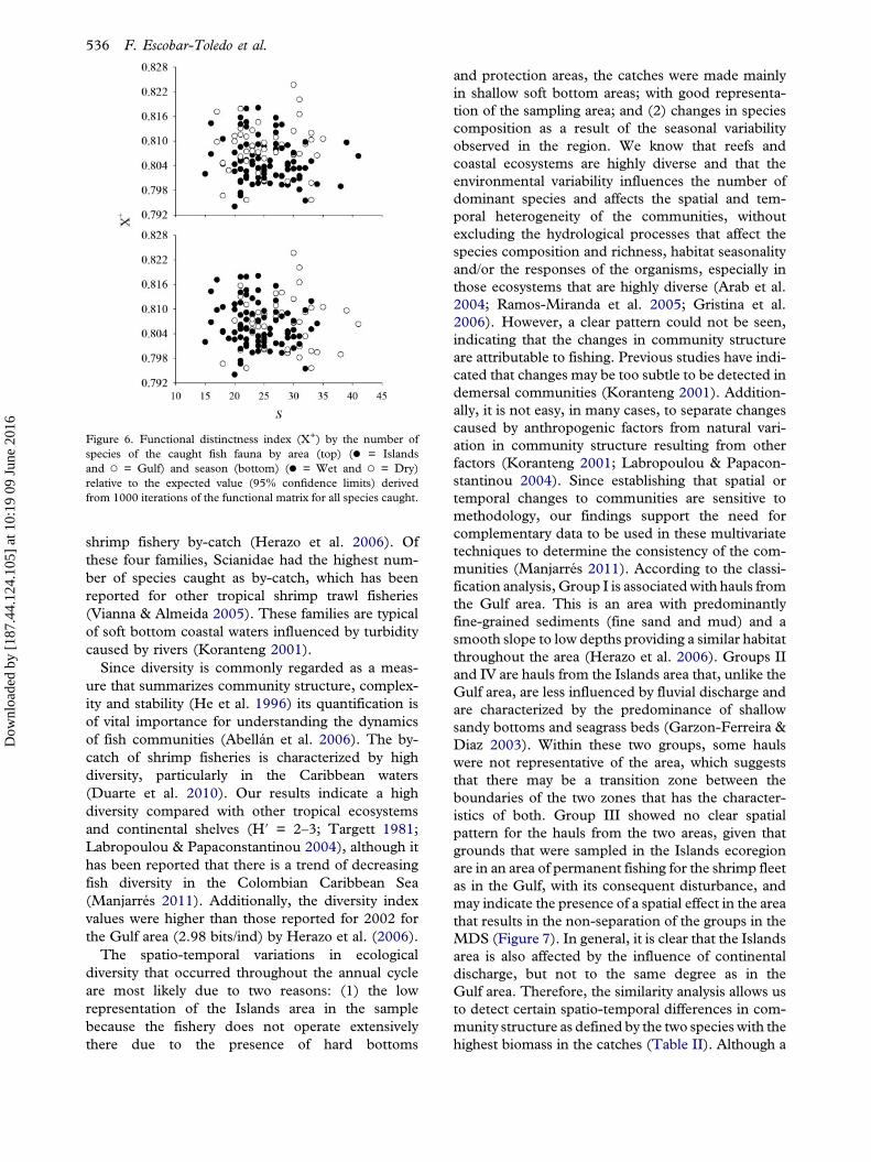
shrimp fishery by-catch (Herazo et al. 2006). Ofthese four families, Scianidae had the highest num-ber of species caught as by-catch, which has beenreported for other tropical shrimp trawl fisheries(Vianna & Almeida 2005). These families are typicalof soft bottom coastal waters influenced by turbiditycaused by rivers (Koranteng 2001).Since diversity is commonly regarded as a meas-
ure that summarizes community structure, complex-ity and stability (He et al. 1996) its quantification isof vital importance for understanding the dynamicsof fish communities (Abellán et al. 2006). The by-catch of shrimp fisheries is characterized by highdiversity, particularly in the Caribbean waters(Duarte et al. 2010). Our results indicate a highdiversity compared with other tropical ecosystemsand continental shelves (H′ = 2–3; Targett 1981;Labropoulou & Papaconstantinou 2004), although ithas been reported that there is a trend of decreasingfish diversity in the Colombian Caribbean Sea(Manjarrés 2011). Additionally, the diversity indexvalues were higher than those reported for 2002 forthe Gulf area (2.98 bits/ind) by Herazo et al. (2006).The spatio-temporal variations in ecological
diversity that occurred throughout the annual cycleare most likely due to two reasons: (1) the lowrepresentation of the Islands area in the samplebecause the fishery does not operate extensivelythere due to the presence of hard bottoms
and protection areas, the catches were made mainlyin shallow soft bottom areas; with good representa-tion of the sampling area; and (2) changes in speciescomposition as a result of the seasonal variabilityobserved in the region. We know that reefs andcoastal ecosystems are highly diverse and that theenvironmental variability influences the number ofdominant species and affects the spatial and tem-poral heterogeneity of the communities, withoutexcluding the hydrological processes that affect thespecies composition and richness, habitat seasonalityand/or the responses of the organisms, especially inthose ecosystems that are highly diverse (Arab et al.2004; Ramos-Miranda et al. 2005; Gristina et al.2006). However, a clear pattern could not be seen,indicating that the changes in community structureare attributable to fishing. Previous studies have indi-cated that changes may be too subtle to be detected indemersal communities (Koranteng 2001). Addition-ally, it is not easy, in many cases, to separate changescaused by anthropogenic factors from natural vari-ation in community structure resulting from otherfactors (Koranteng 2001; Labropoulou & Papacon-stantinou 2004). Since establishing that spatial ortemporal changes to communities are sensitive tomethodology, our findings support the need forcomplementary data to be used in these multivariatetechniques to determine the consistency of the com-munities (Manjarrés 2011). According to the classi-fication analysis, Group I is associated with hauls fromthe Gulf area. This is an area with predominantlyfine-grained sediments (fine sand and mud) and asmooth slope to low depths providing a similar habitatthroughout the area (Herazo et al. 2006). Groups IIand IV are hauls from the Islands area that, unlike theGulf area, are less influenced by fluvial discharge andare characterized by the predominance of shallowsandy bottoms and seagrass beds (Garzon-Ferreira &Diaz 2003). Within these two groups, some haulswere not representative of the area, which suggeststhat there may be a transition zone between theboundaries of the two zones that has the character-istics of both. Group III showed no clear spatialpattern for the hauls from the two areas, given thatgrounds that were sampled in the Islands ecoregionare in an area of permanent fishing for the shrimp fleetas in the Gulf, with its consequent disturbance, andmay indicate the presence of a spatial effect in the areathat results in the non-separation of the groups in theMDS (Figure 7). In general, it is clear that the Islandsarea is also affected by the influence of continentaldischarge, but not to the same degree as in theGulf area. Therefore, the similarity analysis allows usto detect certain spatio-temporal differences in com-munity structure as defined by the two species with thehighest biomass in the catches (Table II). Although a
Figure 6. Functional distinctness index (X+) by the number ofspecies of the caught fish fauna by area (top) (● = Islandsand ○ = Gulf) and season (bottom) (● = Wet and ○ = Dry)relative to the expected value (95% confidence limits) derivedfrom 1000 iterations of the functional matrix for all species caught.
536 F. Escobar-Toledo et al.
Dow
nloa
ded
by [
187.
44.1
24.1
05]
at 1
0:19
09
June
201
6

drastic temporal variation in the composition of thedemersal ichthyofauna of the south-western Colom-bian Caribbean Sea has been reported (Manjarrés2011), our results suggest greater spatial than tem-poral variation in community structure.Diversity indices are clearly disadvantaged relative
to taxonomic diversity indices, as the latter are moresensitive to natural environmental variability and lesssusceptible to variations in sample size (Clarke &Warwick 2001). Although the taxonomic diversityindices have come into use more recently and areconsidered an accurate gauge of biodiversity, somestudies have shown differences in performance.In some cases, they were useful to record relev-ant changes in demersal fish communities (Ramos-Miranda et al. 2005; Gristina et al. 2006), butsometimes they were not able to detect anthropo-genic disturbances (Abellán et al. 2006). However,our results suggest a spatio-temporal difference inthe taxonomic structure of the by-catch fish com-munity. Temporally, the dry season had a lower taxo-nomic distinction and spatially, species have highertaxonomic relationships in the Islands area asopposed to ecological diversity, which showed bothspatial and temporal variation, indicating an influ-ence of environmental variability on the taxonomicrelationships of species in the community. Theseindices have overcome most of the problems of tra-ditional measures of diversity and have been used to
compare degraded and pristine marine areas (Som-erfield et al. 2006). Thus, the low values in thebivariate analysis of taxonomic diversity indices mayindicate that the community structure of the Islandsarea has the lowest diversity of the ichthyofaunaby-catch by being composed of groups of closelyrelated species. This may indicate a reduced respon-siveness of the ichthyofauna in an area prone toenvironmental fluctuations and therefore a loss ofecosystem resilience (Ramos-Miranda et al. 2005).However, as in the case of ecological diversity, thefish community may not be well represented, as theshrimp trawlers do not have access to the entire area.The results suggest that variations in ecological andtaxonomic diversity of the community are more dueto the natural habitat heterogeneity than as a con-sequence of the impact of fishery (Abellán et al.2006; Gristina et al. 2006).
Measuring the functional differences betweenspecies is useful for showing the contribution of eachto the total diversity of the ecosystem. It is knownthat ecosystem functioning is related to the distribu-tion, abundance and biological activity of the speciesassemblage and its functional traits (Naeem &Wright 2003). On the one hand, taxonomic indica-tors relate to the functional diversity of the ecosys-tem and indicate environmental changes (Campbellet al. 2011). However, our results suggest that thebehaviour of taxonomic diversity and functional
Figure 7. Distribution of the hauls in the four groups formed in the analysis of community of the fish by-catch.
Diversity of fish by-catch in the Colombian Caribbean Sea 537
Dow
nloa
ded
by [
187.
44.1
24.1
05]
at 1
0:19
09
June
201
6

diversity were not similar. While the taxonomicdistinctness index values were approximately average,a high percentage of the functional distinctness indexvalues were below the global average. Despite havingfound a relatively high diversity of species in the area,functional distinctness values were low. Moreover, asmall percentage of values fell outside the probabilitydistribution, andmanyotherswere near the lower limit.This might be caused by disturbance of essentialhabitats by trawl vessels in the zone (Jennings et al.2001). Additionally, the Gulf area has the samefunctionality as the Islands area but hosts a greaternumber of species.Thismay be indicative of taxonomicredundancy and thus functional redundancy in theGulf area, but it also suggests that the Islands area is atransition zone between the soft bottom environmentand the hard bottom area (reef). It should be noted thatlow values of functional distinctness in the area mayindicate a decrease in stability and greater sensitivity todisturbances (Bellwood et al. 2003). Thus, any effecton a species in the community could generate a loss ofecosystem function.Finally, the results suggest that the area identified
here as Islands (Gulf area by Díaz-Merlano &Gómez-López 2000) represents differences in thestructure and functional diversity of ichthyofauna incomparison to the Gulf area. This zone may be atransition area between the hard bottom (reef) in theIslands area and the soft bottom of the Gulf area.The two study areas are constantly exploited, so thebiota is more homogeneous within the Gulf area. Inthe Islands area, where some functional groups maybe represented by a small group of species, the func-tional structure would be more vulnerable to humanimpacts and exploitation given its lower structuraland taxonomic diversity (Bellwood et al. 2003).In general, many species caught as by-catch from
shrimp trawl fisheries, which operate year-round, areof conservation relevance or have ecological or eco-nomic value. The fishing affects fish of a wide rangeof sizes, but it mostly affects small fish and makesthem especially vulnerable to overfishing by impact-ing recruitment and growth, which, under constantextraction pressure, could delay population reco-very (Foster & Vincent 2010). Activities commonlyrecommended as actions to reduce the impact of fish-ery on biological communities include by-catchreduction and the establishment of marine pro-tected areas. Our study shows that future manage-ment actions should also consider the spatio-temporalvariability of the demersal fish community structureand diversity, especially in the Islands area, that willallow for the preservation of diversity in the area andwould mitigate the impacts on the biota that may becaused by disruptions to ecosystem processes iffunctional diversity is eroded (Duarte et al. 2010).
Acknowledgements
We thank two anonymous reviewers for their valu-able comments.
Funding
The authors are grateful for the support received fromthe SIP-IPN (grant number 20140981); SEP-CONACyT(grant number 155900); and COLCIENCIAS (grant num-bers 1117-521-29353 and 1117-09-13723), as well as fromthe Instituto Politécnico Nacional through the EDI andCOFAA programmes. FET thanks CONACyT (ConsejoNacional de Ciencia y Tecnología) and IPN-PIFI (InstitutoPolitécnico Nacional) for the scholarship that was pro-vided. MJZR thanks COTEBAL-IPN and CONACyT(grant number 206762).
References
Abellán P, Bilton DT, Millán A, Sánchez-Fernández D, RamsayPM. 2006. Can taxonomic distinctness assess anthropogenicimpacts in inland waters? A case study from a Mediterraneanriver basin. Freshwater Biology 51:1744–56.
Arab A, Lek S, Lounaci A, Park Y. 2004. Spatial and temporalpatterns of benthic invertebrate communities in an intermittentriver (North Africa). Annales de Limnologie – InternationalJournal of Limnology 40:317–27.
Bellido JM, Santos MB, Pennino MG, Valeiras X, Pierce GJ.2011. Fishery discards and bycatch: Solutions for an ecosystemapproach to fisheries management? Hydrobiologia 670:317–33.
Bellwood DR, Hoey AS, Choat JH. 2003. Limited functionalredundancy in high diversity systems: Resilience and ecosystemfunction on coral reefs. Ecology Letters 6:281–85.
Betancur-R. R, Acero A, Bermingham E, Cooke R. 2007.Systematics and biogeography of New World sea catfishes(Siluriformes: Ariidae) as inferred from mitochondrial, nuclear,and morphological evidence. Molecular Phylogenetics andEvolution 45:339–57.
Bianchi G, Gislason H, Graham K, Hill L, Jin X, Koranteng K,et al. 2000. Impact of fishing on size composition and diversityof demersal fish communities. ICES Journal of Marine Science57:558–71.
Campbell N, Neat F, Burns F, Kunzlik P. 2011. Species richness,taxonomic diversity, and taxonomic distinctness of the deep-water demersal fish community on the Northeast Atlanticcontinental slope (ICES Subdivision VIa). ICES Journal ofMarine Science 68:365–76.
Carpenter KE. 2002. The Living Marine Resources of theWestern Central Atlantic. FAO Species Identification Guidefor Fishery Purposes and American Society of Ichthyologistsand Herpetologists Special Publication No. 5. Rome: FAO.2127 pages.
Catchpole TL, Gray TS. 2010. Reducing discards of fish at sea: Areview of European pilot projects. Journal of EnvironmentalManagement 91:717–23.
Cervigón F. 1991. Los Peces Marinos de Venezuela. Caracas:Fundación Científica Los Roques. 415 pages.
Cervigón F. 1993. Los Peces Marinos de Venezuela. Caracas:Fundación Cientifica Los Roques. 497 pages.
Cervigón F. 1994. Los Peces Marinos de Venezuela. Caracas:Fundación Científica Los Roques. 295 pages.
Cervigón F. 1996. Los Peces Marinos de Venezuela. Caracas:Fundación Cientifica Los Roques. 254 pages.
Cervigón F, Cipriani R, Fischer W, Garibaldi L, Hendrickx M,Lemus AJ, et al. 1992. Guía de Campo de las Especies
538 F. Escobar-Toledo et al.
Dow
nloa
ded
by [
187.
44.1
24.1
05]
at 1
0:19
09
June
201
6

Comerciales Marinas y de Aguas Salobres de la CostaSeptentrional de Suramérica. Fichas FAO de Identificaciónde Especies para los Fines de la Pesca. Rome: FAO. 513 pages.
CIOH. 2012. Circulación general de la atmósfera en Colombia.Technical Report CIOH. http://www.cioh.org.co/meteorologia/Climatologia/01-InfoGeneralClimatCaribeCol.pdf (accessed23 October 2013).
Clarke KR. 1993. Non-parametric multivariate analyses ofchanges in community structure. Australian Journal of Ecology18:117–43.
Clarke KR, Warwick RM. 1998. A taxonomic distinctness indexand its statistical properties. Journal of Applied Ecology35:523–31.
Clarke KR, Warwick RM. 2001. Changes in Marine Communit-ies: An Approach to Statistical Analysis and Interpretation. 2ndedition. UK: PRIMER-E Ltd, Plymouth Marine Laboratory.172 pages.
Díaz-Merlano JM, Gómez-López DI. 2000. Programa Nacionalde Investigación en Biodiversidad Marina y Costera (PNIBM).Santa Marta: INVEMAR-FONADE-MMA. 83 pages.
Duarte LO, Gómez-Canchong P, Manjarrés LM, García CB,Escobar FD, Altamar J, et al. 2006. Variabilidad circadiana dela tasa de captura y la estructura de tallas en camarones eictiofauna acompañante en la pesquería de arrastre del MarCaribe de Colombia. Investigaciones Marinas 34:23–42.
Duarte LO, Manjarres L, Escobar F. 2010. Bottom trawl bycatchassessment of the shrimp fishery in the Caribbean Sea offColombia. Proceedings of the Gulf and Caribbean FisheriesInstitute 62:114–19.
Field JG, Clarke KR, Warwick RM. 1982. A practical strategy foranalysing multispecies distribution patterns. Marine EcologyProgress Series 8:37–52.
Foster S, Vincent A. 2010. Tropical shrimp trawl fisheries:Fishers’ knowledge of and attitudes about a doomed fishery.Marine Policy 34:437–46.
Garrido-Linares M, Acero A. 2006. Peces Ophidiiformes delAtlántico occidental tropical con especial énfasis en el MarCaribe colombiano. Biota Colombiana 7:283–99.
Garzon-Ferreira J, Diaz JM. 2003. The Caribbean coral reefs ofColombia. In: Cortés J, editor. Latin American Coral Reefs.Amsterdam: Elsevier Science, p 275–301.
Gristina M, Bahri T, Fiorentino F, Garofalo G. 2006. Compar-ison of demersal fish assemblages in three areas of the Strait ofSicily under different trawling pressure. Fisheries Research81:60–71.
He F, Legendre P, LaFrankie JV. 1996. Spatial pattern of diversityin a tropical rain forest in Malaysia. Journal of Biogeography23:57–74.
Herazo D, Torres A, Olsen E. 2006. Análisis de la composición yabundancia de la ictiofauna presente en la pesca del camarónrosado (Penaeus notialis) en el Golfo de Morrosquillo, CaribeColombiano. Revista MVZ Córdoba 11:47–61.
Jennings S, Dinmore TA, Duplisea DE, Warr KJ, Lancaster JE.2001. Trawling disturbance can modify benthic productionprocesses. Journal of Animal Ecology 70:459–75.
Johnsen JP, Eliasen S. 2011. Solving complex fisheries manage-ment problems: What the EU can learn from the Nordicexperiences of reduction of discards. Marine Policy 35:130–39.
Kaiser MJ, Collie JS, Hall SJ, Jennings S, Poiner IR. 2002.Modification of marine habitats by trawling activities: Pro-gnosis and solutions. Fish and Fisheries 3:114–36.
Kelleher K. 2005. Discards in the World’s Marine Fisheries: AnUpdate. FAO Fisheries Technical Paper no. 470. Rome: FAO.131 pages.
Koranteng KA. 2001. Structure and dynamics of demersalassemblages on the continental shelf and upper slope offGhana, West Africa. Marine Ecology Progress Series 220:1–12.
Labropoulou M, Papaconstantinou C. 2004. Community struc-ture and diversity of demersal fish assemblages: The role offishery. Scientia Marina 68:215–26.
Madrid-Vera J, Amezcua F, Morales-Bojórquez E. 2007. Anassessment approach to estimate biomass of fish communitiesfrom bycatch data in a tropical shrimp-trawl fishery. FisheriesResearch 83:81–89.
Manjarrés L. 2011. Ensamblajes de peces demersales del Caribecolombiano: Patrones espacio-temporales y relación con vari-ables ambientales y pesqueras. Doctoral Thesis. Universidadde Cadiz, España: Facultad de Ciencias del Mar y Ambien-tales. 433 pages.
Naeem S, Wright JP. 2003. Disentangling biodiversity effects onecosystem functioning: Deriving solutions to a seeminglyinsurmountable problem. Ecology Letters 6:567–79.
Nelson JS. 2006. Fishes of the World. 4th edition. Hoboken NJ:John Wiley & Sons, Inc. 601 pages.
Palacios-Salgado D. 2011. Patrones latitudinales de composicióny diversidad funcional de peces asociados a la pesca decamarón del Pacífico mexicano. Doctoral Thesis. CentroInterdisciplinario de Ciencias Marinas, La Paz, Mexico:Instituto Politécnico Nacional. 129 pages.
Pikitch E, Santora E, Babcock A, Bakun A, Bonfil R, Conover D,et al. 2004. Ecosystem-based fishery management. Science305:346–47.
Ramos-Miranda J, Mouillot D, Flores-Hernandez D, Sosa-LopezA, Do-Chi T, Ayala-Perez L. 2005. Changes in four comple-mentary facets of fish diversity in a tropical coastal lagoon after18 years: A functional interpretation. Marine Ecology ProgressSeries 304:1–13.
Ruiz-Ochoa M, Beier E, Bernal G, Barton ED. 2012. Sea surfacetemperature variability in the Colombian Basin, Caribbean Sea.Deep Sea Research I 64:43–53.
Somerfield P, Cochrane S, Dahle S, Pearson T. 2006. Free-livingnematodes and macrobenthos in a high-latitude glacial fjord.Journal of Experimental Marine Biology and Ecology330:284–96.
Somerfield PJ, Clarke KR, Warwick RM, Dulvy NK. 2008.Average functional distinctness as a measure of the compositionof assemblages. ICES Journal of Marine Science 65:1462–68.
Sparre P, Venema SC. 1998. Introduction to Tropical Fish StockAssessment. Part 1. FAO Fisheries Technical Paper 306/1 Rev.2. Rome: FAO. 407 pages.
Targett TE. 1981. Trophic ecology and structure of coastalAntarctic fish communities. Marine Ecology Progress Series4:243–63.
Tonks ML, Griffiths S, Heales DS, Brewer DT, Dell Q. 2008.Species composition and temporal variation of prawn trawlbycatch in the Joseph Bonaparte Gulf, northwestern Australia.Fisheries Research 89:276–93.
Vianna M, Almeida T. 2005. Bony fish bycatch in the southernBrazil pink shrimp (Farfantepenaeus brasiliensis and F. paulensis)fishery. Brazilian Archives of Biology and Technology48:611–23.
Zúñiga H, Altamar J, Manjarrés L. 2004. Caracterización tecno-lógica de la flota de arrastre camaronero del Mar Caribe deColombia. Technical Report: Project GLO/201/GEF. SantaMarta, Colombia: FAO-GEF-UNEP. 21 pages.
Editorial responsibility: Heino Fock
Diversity of fish by-catch in the Colombian Caribbean Sea 539
Dow
nloa
ded
by [
187.
44.1
24.1
05]
at 1
0:19
09
June
201
6

Functional and Structural Food Web Comparison of TerminosLagoon, Mexico in Three Periods (1980, 1998, and 2011)
Isaura Michelle Abascal-Monroy1 & Manuel J. Zetina-Rejón1& Fabián Escobar-Toledo1 &
Gladis A. López-Ibarra1 & Atahualpa Sosa-López2 & Arturo Tripp-Valdez1
Received: 9 April 2015 /Revised: 9 November 2015 /Accepted: 19 November 2015 /Published online: 1 December 2015# Coastal and Estuarine Research Federation 2015
Abstract Terminos Lagoon has a high diversity of speciesand habitats and is the largest coastal lagoon in the southernGulf of Mexico. It has been a natural protected area since1994, but in recent decades, environmental changes havemodified its biological communities and habitats. In thisstudy, we construct three trophic models for the periods1980, 1998, and 2011 using the Ecopath with Ecosim ap-proach to evaluate the status of the ecosystem. Based on mod-el outputs, we compare functional indicators and perform astructural analysis of the food web. We found significantchanges in the biomasses of trophic compartments and in oth-er functional indicators. The global productivity of the eco-system was the main ecosystem indicator that changed overtime. The structural analysis included a collection of centralityindices which measure the number, strength, and distance (interms of number of links) of linkages between each trophiccompartment and all other compartments, as indicators of therelative importance of each compartment in overall energyflows. Structure was also assessed by identifying the number
and composition of subgroups connected by strong trophiclinkages. Certain compartments from lower trophic levels,such as seagrasses, microcrustaceans, meiobenthos, and echi-noderms had the higher values of centrality measures in thethree periods analyzed. Substructures were relatively stablebetween periods, confirming that a reduction in productivitywas the main ecosystem indicator that changed over time.Some trophic compartments were recurrent in substructures,revealing their key role in the food web structure regardless ofchanges in productivity. This analysis suggests that thosecompartments must be prioritized in conservation scenariosbecause the loss of those species would change the ecosystemstructure impacting severely its biological productivity.
Keywords Coastal lagoon . Foodweb . Ecopath . Ecosystemfunctioning . Centrality . Substructures
Introduction
Terminos Lagoon is the largest coastal lagoon in the south-eastern Gulf of Mexico (Fig. 1). Its importance as a nurseryarea for fishes and invertebrates, many of them with commer-cial interest, is well recognized. For this reason, the lagoon isof primary interest for biological conservation and fisheryactivities, and the Mexican government legally declared theTerminos Lagoon ecosystem as a protected area for flora andfauna in 1994. It is also a Ramsar site due to its large areas ofmangroves and associated wetlands. However, the ecosystemhas been subject to severe impacts due to anthropogenic pres-sures during recent decades (Sirot et al. 2015). These pressuresinclude development of the oil industry in the adjacent conti-nental shelf, wetland loss, and mangrove deforestation asso-ciated with crop and livestock development, and urban devel-opment in adjacent areas.
Communicated by James Lovvorn
Electronic supplementary material The online version of this article(doi:10.1007/s12237-015-0054-0) contains supplementary material,which is available to authorized users.
* Manuel J. Zetina-Rejó[email protected]
1 Instituto Politécnico Nacional—Centro Interdisciplinario de CienciasMarinas, Av. IPN S/N Col. Playa Palo Santa Rita, 23096 La Paz, BajaCalifornia Sur, Mexico
2 Instituto de Ecología, Pesquerías y Oceanografía del Golfo deMéxico, Universidad Autónoma de Campeche, Av. Héroe deNacozari 480, 24029 San Francisco de Campeche, Campeche,Mexico
Estuaries and Coasts (2016) 39:1282–1293DOI 10.1007/s12237-015-0054-0
Author's personal copy

Recent studies have highlighted ecological changes forTerminos Lagoon. Using an approach that incorporates waterquality, contaminants in fish, the benthic community, and hab-itat degradation, García-Ríos et al. (2013) evaluated the envi-ronmental condition of the lagoon during 2010. Their resultssuggest that the overall environmental condition of the lagoonwas fair, which means that some indicators like contaminantsin fish and coastal habitat were negatively evaluated.However, Sirot et al. (2015) reported that abiotic parametersshowed very different temporal evolutions over the last threedecades. They found that salinity had increased from 1980 to2011, but pH, depth, and water clarity were very differentduring 1998. No significant changes in temperature were de-tected during the last three decades. Also, Magallanes-Ordóñez et al. (2014) have noted that although elements as-sociated with the presence of oil in sediments are not enrichedin the lagoon, they are present in moderate concentrations.Ramos-Miranda et al. (2005a, b) reported that the loss of di-versity in the fish community was associated with four mainfactors: (1) the fisheries, (2) pollutants from the oil industry,agricultural activities and urban areas (Currie-Alder 2001), (3)habitat degradation by loss of submerged vegetation(seagrass) and mangrove areas, and (4) the loss of estuarineconditions of the lagoon due to the increased contributions ofseawater, which have increased transparency and salinity ofthe lagoon (Villalobos-Zapata et al. 2002). Due to this last fact,in recent years, fish families with a marine affinity, such asMugilidae, Serranidae, Lobotidae, and Achiridae, amongothers, have increased in abundance in the lagoon (Ramos-Miranda et al. 2005a). It has also been reported that the bio-mass of estuarine omnivorous species from intermediate
trophic levels (which dominated the lagoon during the1980s) have been replaced by carnivores and herbivores-detritivores species of marine affinity during 1998 (Sosa-López et al. 2005). However, some species have showed arecovery in their abundances during 2011, and other are stilldecreasing (Sirot et al. 2015). Studies suggest that thesechanges result from the building of reefs nearby and an in-crease in marine conditions that can increase the biomass ofpredators and detritivores. Moreover, a reduction in seagrasscoverage with a consequent decrease in specialist fish speciesthat have a preference for this habitat has also been reported(Villéger et al. 2010).
Changes in biodiversity are usually detected through anal-ysis of the biological communities and are correlated withenvironmental conditions. Those changes in species diversityare supposed to affect ecosystem functioning, for exampleproductivity, resilience, and stability. However, this latter ideais not usually tested due to lack of time series data needed todescribe ecosystem dynamics. To fully understand change andvariability of an ecosystem, it is necessary to evaluate histor-ical conditions and thus visualize future scenarios (Boero et al.2014). Trophic models are usually an alternative to study theresponse of ecosystems to changes in environmental condi-tions. Taking this into account, the main aim of this study wasto compare the function and structure of the Terminos Lagoonecosystem during three different periods with systematicallycollected field data. Specifically, we investigated the differ-ences or similarities in functional indicators and topology ofthe food web. Using an Ecopath with Ecosim (EwE) trophicmodeling approach, we investigate whether the reportedchanges in biological communities and environmental
Fig. 1 Terminos Lagoon at thesoutheastern Gulf of Mexico. Themap shows the sampling stationsused for biological surveys during1980, 1998, and 2011
Estuaries and Coasts (2016) 39:1282–1293 1283
Author's personal copy

conditions are reflected at the ecosystem level, particularly interms of functional indicators and structural properties.
Methods
Study Area
The Terminos Lagoon is located in the southeastern Gulf ofMexico (Fig. 1) and is the largest coastal lagoon in the area,with a surface area of 2500 km2. The lagoon is an estuarinesystem with freshwater discharges from three main rivers: thePalizada (southwest), Chumpan (south), and Candelaria(southeast), which are part of the Usumacinta and Grijalvabasin (the largest fluvial system in Mexico). The lagoon hasan average depth of 3.5 m and is mostly surrounded by man-grove swamps. It is separated from the sea by Carmen Island,but water exchanges with the adjacent continental shelf occurthrough two inlets: Puerto Real in the east (10 m) and ElCarmen in the west (7 m). Three climatic seasons are identi-fied in the region: the winter storms season, which is fromOctober to January; the dry season from February to May;and the rainy season from June to September (Yáñez-Arancibia and Day 1982).
Modeling Approach
We constructed three new trophic models that represent theTerminos Lagoon food web, and they correspond to theyears 1980, 1998, and 2011, which were initially basedon the model previously constructed by Manickhand-Heileman et al. (1998) representing the early 1980s. Eachmodel consists of 41 trophic compartments, 21 morecompartments than the original version. The models werebuilt using the Ecopath with Ecosim (EwE) approach(Christensen et al. 2008), which represents the energyflows between the different biological components of thesystem and consists of a set of linear equations, one foreach trophic compartment, of the form:
Bi⋅P
B
� �i
⋅EEi ¼Xn
j¼1
Bj⋅Q
B
� �j
⋅DC ji þ Bi⋅P
B
� �i
⋅ 1−EEið Þ
þ Y i þ NMi þ BAi
where for an i compartment, Bi is biomass, (P/B)i is theproduction/biomass ratio, EEi is ecotrophic efficiency (thefraction of the production that is used in the system), Bj isthe biomass of predator j, (Q/B)j is the consumption/biomassratio of predator j, DCji is the proportion of prey i in the diet ofpredator j, and Yi is the export value, which in this studyincludes fishery catch when a compartment is exploited.NMi is the net migration rate, and BAi is the biomass
accumulation rate. The last two terms of the equation werenot used in the present study. Based on the equation, inputparameters for each model compartment include B, P/B,Q/B, and EE. Because this equation is balanced, if one param-eter is unknown, it can be estimated from the model.Nevertheless, the diet composition (DCij) of all consumers isrequired to depict all trophic relationships. Additionally, EEivalues must be between 0 and 1, and these values are used tobalance the model. EwE is a relatively simple model for therepresentation of trophic flows and has been widely applied toaquatic ecosystems (http://www.ecopath.org).
Input Data
All input data for the three models were based on field datacollection during three standardized sampling campaigns.Those campaigns were carried on during 12 consecutivemonths in 1980–1981, 1997–1998, and 2010–2011 and rep-resent the more extensive field sampling programs inTerminos Lagoon (Villéger et al. 2010; Sirot et al. 2015).Biological surveys were conducted monthly at 17 samplingstations (Fig. 1) during an annual cycle using a shrimp trawl(5 m long, with an opening mouth of 2.5 m in diameter and amesh size of 19 mm) towed for 12 min at a constant speed of2.5 knots. The identification and diet determination of fisheswere conducted in the laboratory. The diets for non-fish com-partments were taken from the literature (see supplementarymaterial). The biomass estimations for fishes and macroinver-tebrates were made through swept-area survey analysis. Forsome compartments, we let the model estimate their bio-masses to reduce bias due to selectivity of the fishing gear.The P/B ratio is equivalent to total mortality (Allen 1971) andwas estimated as natural mortality following the equation pro-posed by Pauly (1980). For exploited fishes we added to nat-ural mortality the fishing mortality obtained from Zetina-Rejón (2004). TheQ/B ratio was estimated using the empiricalequation proposed by Palomares and Pauly (1998). For non-fish compartments the P/B and Q/B were obtained from theliterature (see supplementary material). The fishery catcheswere taken from the statistical yearbooks. All input data werestandardized in terms of time and area units.
Functional Analysis
The EwE approach calculates several indices that are useful todescribe the functional status of the ecosystem. In this way, weanalyzed the total consumption, total exports, total respiration,and flows to detritus; all of them are part of the total through-put of the food web, which is the sum of all energy flows.Also, the system’s omnivory index (a measure of how feedinginteractions are distributed among trophic levels) and Finn’srecycling index (fraction of total throughput that is recycled)were estimated to describe how energy is used in the food web
1284 Estuaries and Coasts (2016) 39:1282–1293
Author's personal copy
(Christensen et al. 2008). Another indicator was the meantransfer efficiency, which is the geometric mean of energytransfer efficiency between all trophic levels. EwE also esti-mates the ecosystem flow indices proposed by Ulanowicz(1986) to describe the development of an ecosystem, whichincludes the ascendency (A), the development capacity (C),and the overhead (O). The A measures the growth and devel-opment of an ecosystem. The upper limit of A is the develop-ment capacity (C) of the system and is a measure of its poten-tial for growth. The difference between A and C is the over-head (O), which expresses the reserve potential that the systemhas to respond in case of external disturbance. The aboveindices are commonly used in ecosystem analysis based onEwE, and their global patterns have been recently describedby Heymans et al. (2014). Differences in indices between thethree periods were tested using a Friedman test due to the lackof normality and heterogeneous variances in the data.
Structural Analysis
The structural analysis consisted of two parts. In the first part,centrality indices were calculated based on the network topol-ogy, to determine the relative importance of a trophic com-partment in terms of its position in the food web and themagnitude of energy flowing through it. For the calculationof these indices, we considered the consumption flows matrixestimated by the EwE for each of the three different periods(cannibalism flows were not used in the analysis). The firstindex calculated was the weighted degree index (Dw) that isgiven by the sum trophic links weights (flow magnitudes)between a food web compartment i and all other compart-ments in the network (Horvath 2011). Then, we calculatedthe closeness centrality index (Cc), which measures the meaninverse distance (in terms of number of links) between a givencompartment and all other compartments in the network.Higher values of this index indicate greater easy access tothe other network members (Wasserman and Faust 1994).The index is calculated as:
Cci ¼ N−1X N
j¼1di j
where N is the number of trophic compartments in the net-work, and ∑ j=1
N dij is the sum of the shortest path distances(geodesic distances) between the trophic compartment i and j.Finally, we calculated the status index (CKatz) proposed byKatz (1953). This index calculates the relative influence of atrophic compartment within a network, quantifying the flowsnot only with immediate neighbors but also with the trophiccompartments with which it is connected through these imme-diate neighbors. This index can be interpreted as a generaliza-tion of degree centrality (the number of links attached to a
node or trophic compartment), where the number of neighborsat a distance k is also counted but attenuated by αk. This indexis expressed as:
CKatz ið Þ ¼X∞k¼1
XNj¼1
αk Qk� �
ji
where N is the total number of trophic compartments, andQ isthe consumption matrix from EwE. The damping factor αranges from 0 to 1; smaller values reduce the influence oflonger sequences of links, with a value of zero eliminatingall distances greater than a single link. We used an intermedi-ate value of 0.5 (Katz 1953; Junker and Schreiber 2008).Differences in all centrality indices were tested using aKruskal-Wallis test due to the lack of normality and heteroge-neous variances in the data.
The second part of the structural analysis was to identifysubstructures in the food web, which are sets of trophic com-partments that are more highly interconnected to one anotherthan they are with the rest of the network. For this analysis,trophic links were converted into binary and symmetric rela-tions. Binarization consisted of assigning a value of 1 whenthere was a trophic link between two compartments and 0 ifnot. Symmetrization consisted of assigning a value of 1 whentwo food web compartments are related, regardless of direc-tion of trophic flow. We only considered major flows to agiven trophic compartment that were individually ≥20 % oftotal flows to consider substructures based on most importantrelationships. Some authors, such as Junker and Schreiber(2008) and Borgatti et al. (2013), suggest that the number ofsubstructures has to be less than the number of trophic com-partments in the network but also has to be a number manage-able enough to describe the substructures.
We use UCINET 6.2 software for Windows (Borgatti et al.2002) to run substructure identification algorithms. Firstly, weidentify the cliques, which are highly cohesive sets of com-partments among which there are strong connections.Formally in graph theory, a graph (in this study the foodweb) is represented as G=(V, E) formed by a set of V of ver-tices (in this study the trophic compartments) and a set of E ofedges (in this study the trophic links). A subsetU⊆V is said tobe a clique if and only if G(U) is a complete graph, e.g., eachmember of the clique has connections with each other mem-ber. Usually, the minimum size of a clique is considered threevertices. Cliques in a network may overlap, e.g., the samevertex might belong to more than one clique. This analysiscould be used for identifying the importance of a compartmentbased on the number of times that a compartment appears incliques (Wasserman and Faust 1994; Borgatti et al. 2013).Secondly, we applied the analysis of cut points and blocks; thefirst is defined as a trophic compartment that, if removed, willcause the network to be divided into disconnected parts, whichare the blocks (Wasserman and Faust 1994). A subset C⊂V
Estuaries and Coasts (2016) 39:1282–1293 1285
Author's personal copy

is called a cutpoint if the number of blocks ofG–C is larger thanthat of G. A block is a subgraph G′=(V ′, E ′) that is connected(every vertex can be reached from every other vertex) and max-imal (there is no connected subgraphG″=(V″, E″) with V″⊃V ′).A network can havemore than one cutpoint or have no cutpoints.Finally, the lambda sets analysis allows us to identify whichcompartments have connections that, if removed, would resultin disconnected substructures. In this sense, this analysis is usefulfor detecting trophic compartments with key connections. Forvertices u, v ∈V, let λ (u, v) denote the number of edge-disjointpaths (paths with no common edges) between u and v in G; asubset U⊆V is called a lambda set if and only if
minu;v∈U
λ u; vð Þ > maxu∈U ; v∈V−U
λ u; vð Þ
The members of the lambda set have more edge-disjoint paths connecting them to each other than non-members. The lambda set approach allows a ranking ofthe importance of each connection (trophic links) interms of how much of the flows go through each link.It then identifies the sets of relationships that, if discon-nected, would most greatly cut off the flows in the wholenetwork (Brandes and Erlebach 2005; Abarca-Arenaset al. 2007).
Results
Functional Analysis
All input data for the three models and estimated trophic levelsare shown in Table 1, and diet matrices used in modeling canbe found in the supplementary information. Both biomassesand trophic levels differed between years for most groups. Thesummary statistics of the ecosystem models showed differ-ences for the three periods analyzed (Friedman test, p<0.05)(Table 2). The total throughput was higher during 1980 andlower during 2011, indicating a reducing trend, which wassimilarly observed in total consumption, total exports, totalrespiration, and flows to detritus. The total biomass/totalthroughput and system’s omnivory remain relatively stablein all periods. The Finn’s cycling index was also relativelystable but with higher values during 1998. The mean transferefficiency increased during the two last periods, and the highervalue was during 1998.
Figure 2 shows the proportion of the flows in relation tototal throughput. We note a differential use of the energy dur-ing the three periods analyzed. There was an increase in theconsumption flows that indicate a higher demand of energy,but at the expense of an increase in the metabolic cost (totalrespiration flows) and a decrease of the flow to detritus.Additionally, the total exports flows decrease, but this is
mostly related to the establishment of the legal protectionsof the lagoon in 1994, which limits fishery activities.
All ecosystem flow indices significantly decreased from1980 to 2011 (Friedman test, p<0.05) (Table 2). Comparedto 1980, the ascendency (A) showed a decrease of 38 and 56%during 1998 and 2011, respectively. Similarly, the develop-ment capacity (C) had a decrease of 31 and 53 % during1998 and 2011, respectively. However, the relative ascenden-cy (A/C), which is an index of organization of the food web,was 0.4, 0.35, and 0.38 for 1980, 1998, and 2011, respective-ly. This suggests that in somemanner, the structure of the foodweb did not change, despite an overall decline of 58 % in totalthroughput and 60 % in total primary production.
Structural Analysis
In Fig. 3, we show the ranking order of trophic compartmentsbased on the application of centrality indices. We found that inall the models, four of the five compartments with the highestweighted degree index of weighted degree index were thesame, although, we observed differences between years in therelative ranking. A Kruskal-Wallis test including all of 41 tro-phic compartments revealed no significant differences in rank-ing between years (p>0.05). In the case of closeness centralityindex, we found that three of the five trophic compartmentsshowing the highest value were the same, but their rankingsalso differed between years; the Kruskal-Wallis test revealedsignificant differences between years in ranking for all com-partments (p<0.05). Finally, for the status index (CKatz), it wasfound that in the 3 years, four of the compartments with thehighest status percentage were the same, changing only theirrelative ranking between years. In this case, the Kruskal-Wallistest showed no significant differences in rankings among allcompartments between years (p>0.05).
Over the 3 years analyzed, the number of cliques declined,as did the number and percentage of all compartments thatwere within cliques (Table 3). Nevertheless, four cliques werepresent in each of the 3 years, and three trophic compartments(meiobenthos, seagrasses, and mollusks) were part of two tothree of these cliques (Table 4). This pattern indicates thatthese benthic organisms at lower trophic levels were especial-ly important to the food web.
In analyses of cutpoints and blocks, six cutpoints were thesame in each year, while phytoplankton was a cutpoint only in1980 (Table 3). If these cutpoints were removed, the food webwould be divided into 14 isolated blocks in 1980, 14 in 1998,and 12 in 2011. This pattern indicates that the food web iscomplex in terms of number of blocks, but that this complex-ity was reduced in 2011.
The analysis of lambda sets revealed that seagrasses playsan important role in maintaining food web structure during thethree periods. In 1980, the relationship between seagrassesand meiobenthos was the most important, but for 1998 and
1286 Estuaries and Coasts (2016) 39:1282–1293
Author's personal copy
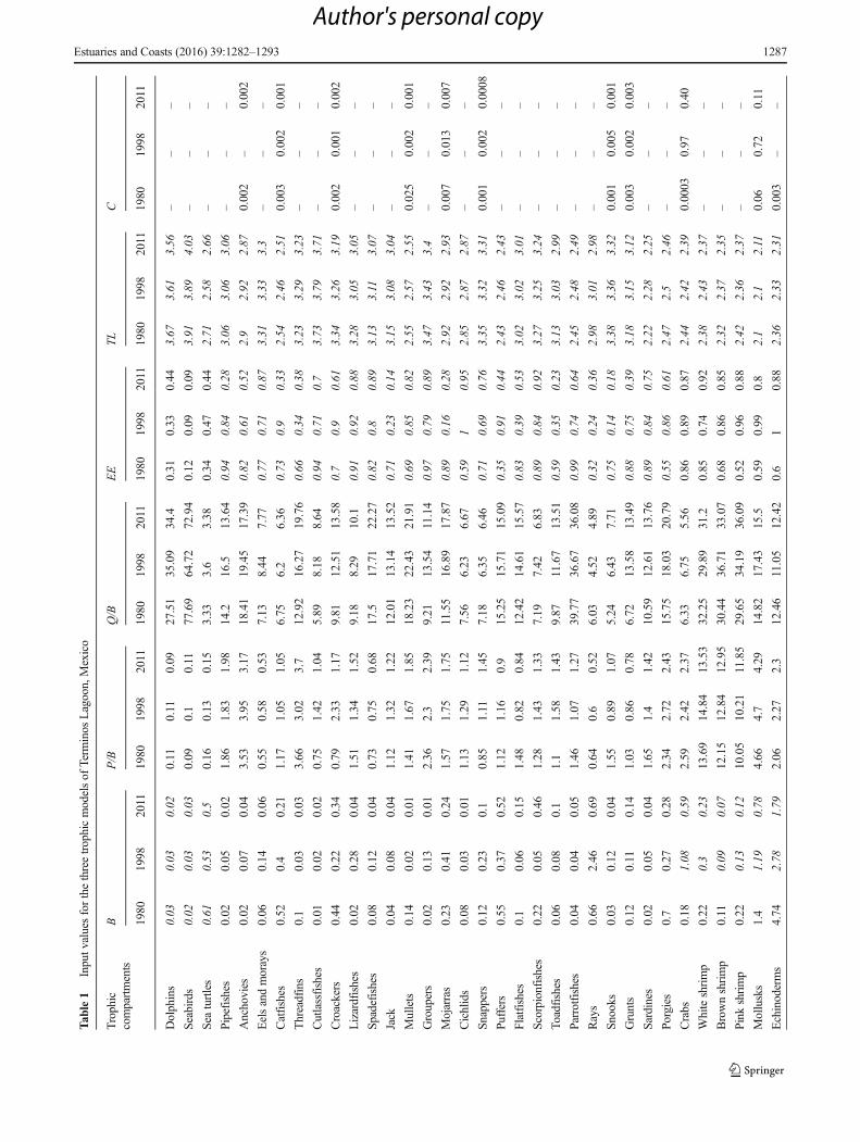
Tab
le1
Inputv
aluesforthethreetrophicmodelsof
Term
inos
Lagoon,Mexico
Trophic
compartments
BP/B
Q/B
EE
TLC
1980
1998
2011
1980
1998
2011
1980
1998
2011
1980
1998
2011
1980
1998
2011
1980
1998
2011
Dolphins
0.03
0.03
0.02
0.11
0.11
0.09
27.51
35.09
34.4
0.31
0.33
0.44
3.67
3.61
3.56
––
–
Seabirds
0.02
0.03
0.03
0.09
0.1
0.11
77.69
64.72
72.94
0.12
0.09
0.09
3.91
3.89
4.03
––
–
Sea
turtles
0.61
0.53
0.5
0.16
0.13
0.15
3.33
3.6
3.38
0.34
0.47
0.44
2.71
2.58
2.66
––
–
Pipefishes
0.02
0.05
0.02
1.86
1.83
1.98
14.2
16.5
13.64
0.94
0.84
0.28
3.06
3.06
3.06
––
–
Anchovies
0.02
0.07
0.04
3.53
3.95
3.17
18.41
19.45
17.39
0.82
0.61
0.52
2.9
2.92
2.87
0.002
–0.002
Eelsandmorays
0.06
0.14
0.06
0.55
0.58
0.53
7.13
8.44
7.77
0.77
0.71
0.87
3.31
3.33
3.3
––
–
Catfishes
0.52
0.4
0.21
1.17
1.05
1.05
6.75
6.2
6.36
0.73
0.9
0.33
2.54
2.46
2.51
0.003
0.002
0.001
Threadfins
0.1
0.03
0.03
3.66
3.02
3.7
12.92
16.27
19.76
0.66
0.34
0.38
3.23
3.29
3.23
––
–
Cutlassfishes
0.01
0.02
0.02
0.75
1.42
1.04
5.89
8.18
8.64
0.94
0.71
0.7
3.73
3.79
3.71
––
–
Croackers
0.44
0.22
0.34
0.79
2.33
1.17
9.81
12.51
13.58
0.7
0.9
0.61
3.34
3.26
3.19
0.002
0.001
0.002
Lizardfishes
0.02
0.28
0.04
1.51
1.34
1.52
9.18
8.29
10.1
0.91
0.92
0.88
3.28
3.05
3.05
––
–
Spadefishes
0.08
0.12
0.04
0.73
0.75
0.68
17.5
17.71
22.27
0.82
0.8
0.89
3.13
3.11
3.07
––
–
Jack
0.04
0.08
0.04
1.12
1.32
1.22
12.01
13.14
13.52
0.71
0.23
0.14
3.15
3.08
3.04
––
–
Mullets
0.14
0.02
0.01
1.41
1.67
1.85
18.23
22.43
21.91
0.69
0.85
0.82
2.55
2.57
2.55
0.025
0.002
0.001
Groupers
0.02
0.13
0.01
2.36
2.3
2.39
9.21
13.54
11.14
0.97
0.79
0.89
3.47
3.43
3.4
––
–
Mojarras
0.23
0.41
0.24
1.57
1.75
1.75
11.55
16.89
17.87
0.89
0.16
0.28
2.92
2.92
2.93
0.007
0.013
0.007
Cichlids
0.08
0.03
0.01
1.13
1.29
1.12
7.56
6.23
6.67
0.59
10.95
2.85
2.87
2.87
––
–
Snappers
0.12
0.23
0.1
0.85
1.11
1.45
7.18
6.35
6.46
0.71
0.69
0.76
3.35
3.32
3.31
0.001
0.002
0.0008
Puffers
0.55
0.37
0.52
1.12
1.16
0.9
15.25
15.71
15.09
0.35
0.91
0.44
2.43
2.46
2.43
––
–
Flatfishes
0.1
0.06
0.15
1.48
0.82
0.84
12.42
14.61
15.57
0.83
0.39
0.53
3.02
3.02
3.01
––
–
Scorpionfishes
0.22
0.05
0.46
1.28
1.43
1.33
7.19
7.42
6.83
0.89
0.84
0.92
3.27
3.25
3.24
––
–
Toadfishes
0.06
0.08
0.1
1.1
1.58
1.43
9.87
11.67
13.51
0.59
0.35
0.23
3.13
3.03
2.99
––
–
Parrotfishes
0.04
0.04
0.05
1.46
1.07
1.27
39.77
36.67
36.08
0.99
0.74
0.64
2.45
2.48
2.49
––
–
Rays
0.66
2.46
0.69
0.64
0.6
0.52
6.03
4.52
4.89
0.32
0.24
0.36
2.98
3.01
2.98
––
–
Snooks
0.03
0.12
0.04
1.55
0.89
1.07
5.24
6.43
7.71
0.75
0.14
0.18
3.38
3.36
3.32
0.001
0.005
0.001
Grunts
0.12
0.11
0.14
1.03
0.86
0.78
6.72
13.58
13.49
0.88
0.75
0.39
3.18
3.15
3.12
0.003
0.002
0.003
Sardines
0.02
0.05
0.04
1.65
1.4
1.42
10.59
12.61
13.76
0.89
0.84
0.75
2.22
2.28
2.25
––
–
Porgies
0.7
0.27
0.28
2.34
2.72
2.43
15.75
18.03
20.79
0.55
0.86
0.61
2.47
2.5
2.46
––
–
Crabs
0.18
1.08
0.59
2.59
2.42
2.37
6.33
6.75
5.56
0.86
0.89
0.87
2.44
2.42
2.39
0.0003
0.97
0.40
Whiteshrimp
0.22
0.3
0.23
13.69
14.84
13.53
32.25
29.89
31.2
0.85
0.74
0.92
2.38
2.43
2.37
––
–
Brownshrimp
0.11
0.09
0.07
12.15
12.84
12.95
30.44
36.71
33.07
0.68
0.86
0.85
2.32
2.37
2.35
––
–
Pink
shrimp
0.22
0.13
0.12
10.05
10.21
11.85
29.65
34.19
36.09
0.52
0.96
0.88
2.42
2.36
2.37
––
–
Mollusks
1.4
1.19
0.78
4.66
4.7
4.29
14.82
17.43
15.5
0.59
0.99
0.8
2.1
2.1
2.11
0.06
0.72
0.11
Echinoderms
4.74
2.78
1.79
2.06
2.27
2.3
12.46
11.05
12.42
0.6
10.88
2.36
2.33
2.31
0.003
––
Estuaries and Coasts (2016) 39:1282–1293 1287
Author's personal copy

2011, we found that the relationship between seagrasses andmicrocrustaceans was the most important (Table 3).
Discussion
Our results clearly indicate significant differences in function-al indicators and but not necessarily in structure. We foundthat biomasses of trophic compartments were different in thethree models. Most of the fish biomasses were systematicallyobtained from field data during the three periods analyzed,which indicated that the production level of the ecosystemchanged. Some field studies have also confirmed a reductionin biomass in primary producers such as the seagrasses(Herrera-Silveira et al. 2011) in addition to those that reportedbiomass reductions in fishes from lower trophic levels(Ramos-Miranda et al. 2005a) and increases for fishes fromhigher trophic levels (Sosa-López et al. 2005). In this sense,Sirot et al. (2015) reported that the occurrence and abundanceof most dominant species changed markedly over the threeperiods studied here.
Ecosystem indices revealed a diminishing trend from 1998to 2011 in the magnitude of energy flows, which means thatthe ecosystem has been degraded in the last decades in termsof its biological production. Odum (1969) suggests that ma-ture ecosystems show higher recycling levels than immatureecosystems, which implies a positive trend as ecosystems de-velop. However, tropical coastal lagoons are continuously re-ceiving external nutrients, so recycling is not necessarily great.In addition, they are relatively small systems, and it has beenfound that recycling is lower in small systems and higher inlarger systems (Heymans et al. 2014). Our results suggest thataltered conditions during 1998 in Terminos Lagoon werereflected in to the higher recycling, which could possibly in-dicate a change in nutrient inputs and increased metaboliccosts (respiration flows). During 1998, a high intensity ElNiño Southern Oscillation (ENSO) event occurred and it hasbeen reported that the influence of this phenomenon couldaffect the streamflow and sediment load of the UsumacintaRiver, particularly increasing the water and sediment dis-charges during warm conditions (Muñoz-Salinas andCastillo 2015). In this sense, an increase in nutrients couldresulted in the increased biomass of fishes from higher trophiclevels reported by Sosa-López et al. (2005) increasing themean transfer energy during 1998. This could also be thereason for the increase in energy demands (consumptionflows).
Ulanowicz (1986) suggests that ascendency increases dur-ing ecosystem evolution. Our results show that TerminosLagoon exhibited a decreasing trend in ascendency.However, the relative ascendency was generally stable. Theascendency is estimated as the product of total systemthroughput and the average mutual information (AMI). TheT
able1
(contin
ued)
Trophic
compartments
BP/B
Q/B
EE
TLC
1980
1998
2011
1980
1998
2011
1980
1998
2011
1980
1998
2011
1980
1998
2011
1980
1998
2011
Microcrustaceans
1.76
1.36
1.05
12.56
10.43
10.47
35.03
38.76
34.87
0.56
0.81
0.93
2.1
2.11
2.1
––
–
Polychaetes
8.92
7.12
4.23
4.26
3.87
420.12
21.15
18.35
0.33
0.56
0.6
2.07
2.07
2.07
––
–
Meiobenthos
3.02
3.14
2.02
10.67
11.63
10.79
46.04
45.39
47.57
0.94
0.78
0.85
2.04
2.05
2.05
––
–
Zooplankton
1.13
0.52
0.3
19.84
18.99
18.41
71.78
80.78
71.14
0.48
0.8
0.91
2.03
2.04
2.04
––
–
Seagrasses
180.19
101.97
85.3
8.87
9.63
8.43
––
–0.04
0.05
0.05
11
1–
––
Phytoplankton
154.6
55.85
39.18
3.45
3.86
3.55
––
–0.14
0.17
0.14
11
1–
––
Detritus
84.71
84.71
84.71
––
––
––
0.18
0.28
0.24
11
1–
––
The
datain
italic
wereestim
ated
bythemodel
.Bbiom
ass(t•km
2),P/B
productio
n/biom
ass(year−1),Q/B
consum
ption/biom
ass(year−1),EEecotrophicefficiency,T
Ltrophiclevel,Ccatch(t•km
2)
1288 Estuaries and Coasts (2016) 39:1282–1293
Author's personal copy

latter represents the internal organization of the food web tak-ing into account the extent to which energy is channeled alongdifferent trophic links to minimize energy loss (Ulanowiczet al. 2009). In this sense, the total throughput could be themain reason for the reduction in the ascendency because itdecreased significantly from 1980 to 2011.
In food webs, the topological centrality has been related tothe idea of key roles in food webs (Solé and Montoya 2001;Dunne et al. 2002; Bauer et al. 2010). This idea suggests thatspecies with a high number of links or an important position inthe topological pathways could be considered as keystonespecies (Albert et al. 2000). We found that for the three pe-riods, the most important compartments in the case of theweighted degree index were the same, which belongs to lowertrophic levels (TL=1 and TL=2). Vasas et al. (2007) suggested
that compartments such as primary producers and, in somecases, primary consumers appear as those with more connec-tions, which could indicate a bottom-up flow control in thefood web.
The closeness centrality index showed that in the threeperiods, the compartments that presented the highest valueswere similar; however, the differences in the ranking of somecompartments were significant. For 1980 and 1998, mulletsexhibited the highest closeness index, while for 2011,anchovies exhibited the highest value, displacing mullets tothe fourth place in ranking order. Borgatti et al. (2002) men-tioned that the trophic compartments showing higher values ofthis index are those with greater access to other compartmentsof the network. Additionally, Borgatti and Foster (2003) sug-gest that compartments with the highest values interact withothers compartments without the intervention of intermediarycompartments. Although mullets and anchovies are from sim-ilar trophic levels, their feeding is quite different. Mulletsmostly feed on detritus, while anchovies feed on phytoplank-ton. This could indicate that the importance of the primarysources of energy to the food web has been different in theperiods studied.
The status indices showed that, for 1980 and 1998, zoo-plankton was the compartment with the highest value.However, during 2011, the microcrustaceans exhibited thehighest value, moving the zooplankton to the second rank,but with no significant differences in ranking overall 41 tro-phic compartments. This indicates that compartments fromlower trophic levels have a large influence on other compart-ments that are either direct neighbors or indirect neighbors(Katz 1953). We found that this index identified almost thesame compartments as the degree index as being the mostimportant, but rather in terms of their indirect effects on othercompartments. Those results reinforce the idea that the foodweb of the Terminos Lagoon ecosystem could have a bottom-
Table 2 Summary statistics forthree trophic models of TerminosLagoon, Mexico. Theseparameters are defined inmethods section
Parameter 1980 1998 2011 Units
Total system throughput 4926 2972 2080 t/km2/year
Total consumption 611.99 521.57 331.34 t/km2/year
Total exports 1790.08 900.69 671.51 t/km2/year
Total respiration 345.69 301.01 191.03 t/km2/year
Sum of flows to detritus 2178.27 1248.35 885.92 t/km2/year
Total biomass / total throughput 0.07 0.06 0.07 t/km2/year
Total primary production 2131.5 1197.5 858.3 t/km2/year
System’s omnivory index 0.24 0.22 0.22 -
Finn’s cycling index 3.04 4.32 3.65 %
Mean transfer efficiency 11.40 13.80 13.10 %
Ascendency 5918.3 3667.4 2579.7 flow bits
Overhead 9013.8 6704.0 4444.9 flow bits
Development capacity 14932.1 10371.4 7024.6 flow bits
Relative ascendency 0.396 0.353 0.367
0
0.1
0.2
0.3
0.4
0.5
TC/TST TE/TST TR/TST FD/TST
Pro
port
ion
1980
1998
2011
Fig. 2 Comparison of energy flow use in Terminos Lagoon models forthree periods (1980, 1998, and 2011). TST total throughput, TC totalconsumption, TE total exports, TR total respiration, and FD flows todetritus
Estuaries and Coasts (2016) 39:1282–1293 1289
Author's personal copy

up flow control. This index has not been previously applied tofood webs network data, but it has been shown that it has nonumber of links dependency, which means that a high numberof links does not necessarily imply a high influence (Grindrodet al. 2011). Therefore, we consider the status index could beuseful for exploring the relative importance of a compartmentin the food web based on the influence they have on the rest ofthe compartments.
In the case of the substructures, we found a reduction thenumber of cliques from 1980 to 2011. However, four cliqueswere recurrent during the three periods analyzed, suggestingthat these substructures are important to maintaining the struc-ture of the food web. It has been suggested that such substruc-tures can reduce the spread of disturbances through the
network due to the relatively high internal connectivity inrelation to the rest of the network. (Krause et al. 2003; Tengand McCann 2004; Rezende et al. 2009; Stouffer andBascompte 2011). In the case of the Terminos Lagoon ecosys-tem, these four cliques can help stabilize the network eventhough there are changes in its functioning. Additionally, if anode appears more frequently in the cliques, its trophic rolewill be more important for the connectivity and functioning ofthe entire food web. In this sense, seagrasses were the mostrecurrent clique compartment, followed bymeiobenthos, mol-lusks, and polychaetes.
In the cutpoints and blocks analysis, we found that thecutpoints were trophic compartments from lower trophiclevels, while primary producers and primary consumers
1980 1998 2011
Weighted
degree Index
Closeness
centrality
Index
Status Index
Fig. 3 Relative position in ranking order of centrality indices during thethree periods analyzed (1980, 1998, and 2011). Only the names of trophiccompartments with the highest value of indices are indicated. The linesrepresent the trophic links between compartments, and the center of thecircular diagram represents the highest value of the index and decreasestowards its periphery. Weighted degree index is the sum of flowmagnitudes between a given trophic compartment and all other
compartments in the food web, closeness centrality index is the meaninverse distance (in terms of number of links) between a givencompartment and all other compartments, and status index is the sum offlows from a given compartment to all other compartments, with eachflow weighted by a value that declines with increasing numbers of linksthat separate the compartments
1290 Estuaries and Coasts (2016) 39:1282–1293
Author's personal copy
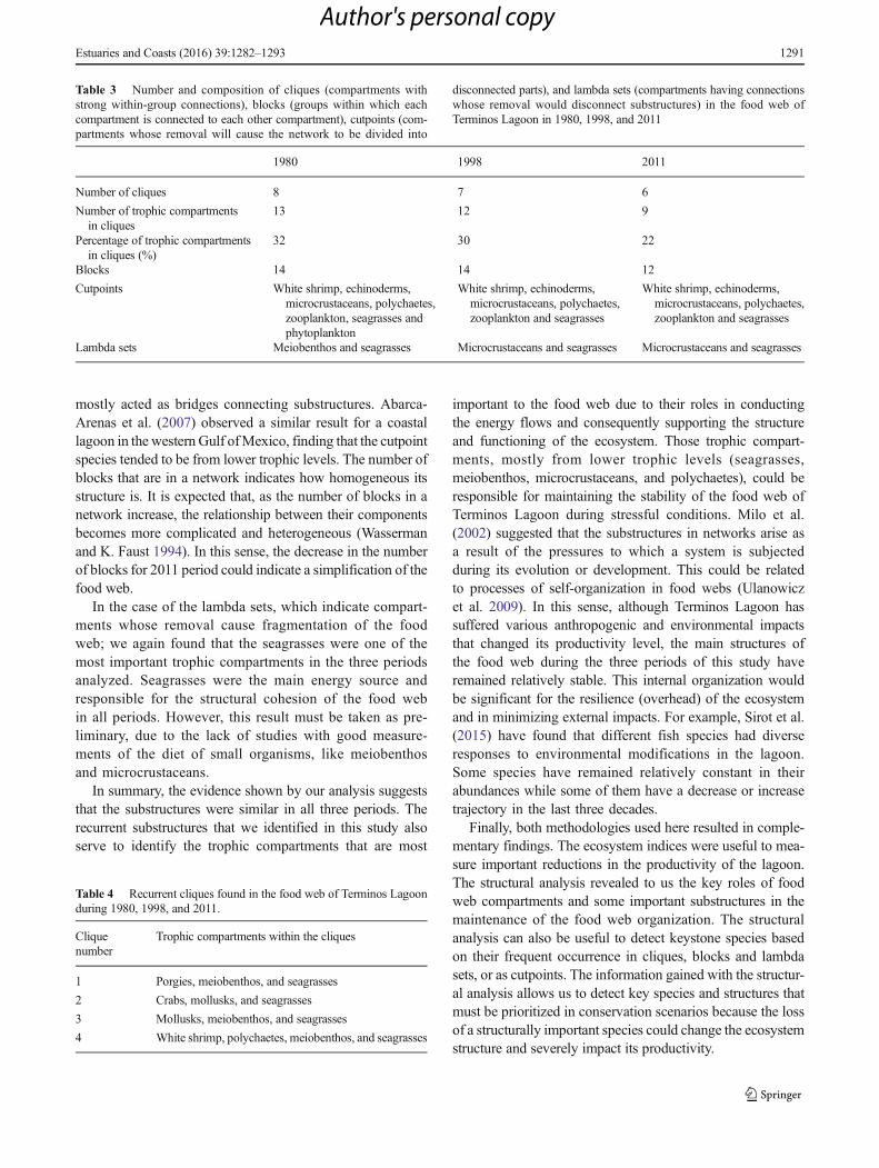
mostly acted as bridges connecting substructures. Abarca-Arenas et al. (2007) observed a similar result for a coastallagoon in the western Gulf ofMexico, finding that the cutpointspecies tended to be from lower trophic levels. The number ofblocks that are in a network indicates how homogeneous itsstructure is. It is expected that, as the number of blocks in anetwork increase, the relationship between their componentsbecomes more complicated and heterogeneous (Wassermanand K. Faust 1994). In this sense, the decrease in the numberof blocks for 2011 period could indicate a simplification of thefood web.
In the case of the lambda sets, which indicate compart-ments whose removal cause fragmentation of the foodweb; we again found that the seagrasses were one of themost important trophic compartments in the three periodsanalyzed. Seagrasses were the main energy source andresponsible for the structural cohesion of the food webin all periods. However, this result must be taken as pre-liminary, due to the lack of studies with good measure-ments of the diet of small organisms, like meiobenthosand microcrustaceans.
In summary, the evidence shown by our analysis suggeststhat the substructures were similar in all three periods. Therecurrent substructures that we identified in this study alsoserve to identify the trophic compartments that are most
important to the food web due to their roles in conductingthe energy flows and consequently supporting the structureand functioning of the ecosystem. Those trophic compart-ments, mostly from lower trophic levels (seagrasses,meiobenthos, microcrustaceans, and polychaetes), could beresponsible for maintaining the stability of the food web ofTerminos Lagoon during stressful conditions. Milo et al.(2002) suggested that the substructures in networks arise asa result of the pressures to which a system is subjectedduring its evolution or development. This could be relatedto processes of self-organization in food webs (Ulanowiczet al. 2009). In this sense, although Terminos Lagoon hassuffered various anthropogenic and environmental impactsthat changed its productivity level, the main structures ofthe food web during the three periods of this study haveremained relatively stable. This internal organization wouldbe significant for the resilience (overhead) of the ecosystemand in minimizing external impacts. For example, Sirot et al.(2015) have found that different fish species had diverseresponses to environmental modifications in the lagoon.Some species have remained relatively constant in theirabundances while some of them have a decrease or increasetrajectory in the last three decades.
Finally, both methodologies used here resulted in comple-mentary findings. The ecosystem indices were useful to mea-sure important reductions in the productivity of the lagoon.The structural analysis revealed to us the key roles of foodweb compartments and some important substructures in themaintenance of the food web organization. The structuralanalysis can also be useful to detect keystone species basedon their frequent occurrence in cliques, blocks and lambdasets, or as cutpoints. The information gained with the structur-al analysis allows us to detect key species and structures thatmust be prioritized in conservation scenarios because the lossof a structurally important species could change the ecosystemstructure and severely impact its productivity.
Table 3 Number and composition of cliques (compartments withstrong within-group connections), blocks (groups within which eachcompartment is connected to each other compartment), cutpoints (com-partments whose removal will cause the network to be divided into
disconnected parts), and lambda sets (compartments having connectionswhose removal would disconnect substructures) in the food web ofTerminos Lagoon in 1980, 1998, and 2011
1980 1998 2011
Number of cliques 8 7 6
Number of trophic compartmentsin cliques
13 12 9
Percentage of trophic compartmentsin cliques (%)
32 30 22
Blocks 14 14 12
Cutpoints White shrimp, echinoderms,microcrustaceans, polychaetes,zooplankton, seagrasses andphytoplankton
White shrimp, echinoderms,microcrustaceans, polychaetes,zooplankton and seagrasses
White shrimp, echinoderms,microcrustaceans, polychaetes,zooplankton and seagrasses
Lambda sets Meiobenthos and seagrasses Microcrustaceans and seagrasses Microcrustaceans and seagrasses
Table 4 Recurrent cliques found in the food web of Terminos Lagoonduring 1980, 1998, and 2011.
Cliquenumber
Trophic compartments within the cliques
1 Porgies, meiobenthos, and seagrasses
2 Crabs, mollusks, and seagrasses
3 Mollusks, meiobenthos, and seagrasses
4 White shrimp, polychaetes, meiobenthos, and seagrasses
Estuaries and Coasts (2016) 39:1282–1293 1291
Author's personal copy
Acknowledgments We are grateful to the projects SEP-CONACyT:155900 and ANR-CONACyT:111465 for their financial sup-port. MJZR and ATV thanks EDI and COFAA from Instituto PolitécnicoNacional, COTEBAL-IPN and CONACyT grant 206762. IMAM and FETthankCONACyTand IPN for the scholarship thatwas provided.We thank tothe two anonymous reviewers for their constructive comments.
References
Abarca-Arenas, L.G., J. Franco-López, M.S. Peterson, N.J. Brown-Peterson, and E. Valero-Pacheco. 2007. Sociometric analysis ofthe role of penaeids in the continental shelf food web off Veracruz,Mexico based on by-catch. Fisheries Research 87: 46–57.
Albert, R., H. Jeong, and A.L. Barabási. 2000. Error and attack toleranceof complex networks. Nature 406: 378–381.
Allen, K.R. 1971. Relation between production and biomass. Journal ofthe Fisheries Research Board of Canada 28: 1573–1581.
Bauer, B., F. Jordán, and J. Podani. 2010. Node centrality indices in foodwebs: Rank orders versus distributions. Ecological Complexity 7:471–477.
Boero, F., A. C. Kraberg, G. Krause and K.H. Wiltshire. 2014. Time is anaffliction: why ecology cannot be as predictive as physics and why itneeds time series. Journal of Sea Research (In press).
Borgatti, S.P., and P.C. Foster. 2003. The network paradigm in organiza-tional research: A review and typology. Journal of Management 29:991–1013.
Borgatti S.P., M.G. Everett and J.C. Johnson. 2013. Analyzing SocialNetworks. Sage Publications
Borgatti, S.P., M.G. Everett and L.C. Freeman. 2002. Ucinet 6 forWindows: Software for Social Network Analysis Harvard:Analytic Technologies
Brandes, U. and T. Erlebach. 2005. Network analysis: methodologicalfoundations (Vol. 3418). Springer Science and Business Media
Christensen, V., C. J. Walters, D. Pauly, and R. Forrest. 2008. Ecopathwith Ecosim version 6: user guide. In: Lenfest Ocean FuturesProject, Vancouver, Canada, 235p
Currie-Alder, B.A.B. 2001. Collaborative management of the Mexicancoast. Public participation and oil industry in the Terminos LagoonProtected Area. MSc thesis. Simon Fraser University, Burnaby, BC
Dunne, J.A., R.J. Williams, and N.D. Martinez. 2002. Network structureand biodiversity loss in food webs: Robustness increases withconnectance. Ecology Letters 5: 558–567.
García-Ríos, V., L. Alpuche-Gual, J. Herrera-Silveira, J. Montero-Muñoz, S. Morales-Ojeda, D. Pech, M.F. Cepeda-González, O.Zapata-Pérez, and G. Gold-Bouchot. 2013. EnvironmentalDevelopment 7: 72–79.
Grindrod, P., M.C. Parsons, D.J. Higham, and E. Estrada. 2011.Communicability across evolving networks. Physical Review E83: 046120.
Herrera-Silveira, J.A., L. Arellano-Méndez and S. Morales-Ojeda. 2011.Report of the Pilot Project Natural Habitat and EcosystemConservation of Coastal and Marine Zones of the Gulf of Mexico:seagrass beds characterization for restoration pilot project: PhaseI-2011
Heymans, J.J., M. Coll, S. Libralato, L. Morissette, and V. Christensen.2014. Global patterns in ecological indicators of marine food webs:A modelling approach. PloS One 9, e95845.
Horvath, S. 2011. Weighted network analysis: Applications in genomicsand systems biology, 1st ed. New York: Springer.
Junker, B. H. and F. Schreiber. 2008. Analysis of Biological Networks .John Wiley & Sons. 346p.
Katz, L. 1953. A new status index derived from sociometric analysis.Psychometrika 18: 39–43
Krause, A.E., K.A. Frank, D.M. Mason, R.E. Ulanowicz, and W.W.Taylor. 2003. Compartments revealed in food-web structure.Nature 426: 282–285.
Magallanes-Ordóñez, V.R., A.J. Marmolejo-Rodríguez, G.M. Rodríguez-Figueroa, A. Sánchez-González, S. Aguíñiga-García, F. Arreguın-Sánchez, M.J. Zetina-Rejón, A. Tripp-Valdez, and J.A. Romo-Ríos.2014. Estuarine, coastal and shelf science. Estuarine Coastal andShelf Science 156: 116–123.
Manickhand-Heileman, S.F., A. Arreguı n-Sánchez, and L. Lara-Dominguez Soto. 1998. Energy flow and network analysis ofTerminos Lagoon, SW Gulf of Mexico. Journal of Fish Biology53: 179–197.
Milo, R., S. Shen-Orr, S. Itzkovitz, N. Kashtan, D. Chklovskii, and U.Alon. 2002. Network motifs: Simple building blocks of complexnetworks. Science 298: 824–827.
Muñoz-Salinas, E., and M. Castillo. 2015. Streamflow and sediment loadassessment from 1950 to 2006 in the Usumacinta and Grijalva Rivers(Southern Mexico) and the influence of ENSO. Catena 127: 270–278.
Odum, E.P. 1969. The strategy of ecosystem development. Science 104:262–270.
Palomares, M.L., and D. Pauly. 1998. Predicting food consumption of fishpopulations as functions of mortality, food type, morphometrics, tem-perature and salinity.Marine and Freshwater Research 49: 447–453.
Pauly, D. 1980. On the interrelationships between natural mortality,growth parameters and mean environmental temperatures in its fishstocks. Journal du Conseil International pour l’Exploration de laMer 39: 175–192.
Ramos-Miranda, J., D. Mouillot, D. Flores-Hernández, A. Sosa-López, T.Do-Chi, and L. Ayala-Pérez. 2005a. Changes in four complementaryfacets of fish diversity in a tropical coastal lagoon after 18 years: Afunctional interpretation.Marine Ecology Progress Series 304: 1–13.
Ramos-Miranda, J.L., D. Quiniou, T. Flores-Hernández, T. Do Chi, L.Ayala Pérez, and A. Sosa-Lopez. 2005b. Spatial and temporalchanges in the nekton of the Terminos Lagoon, Campeche,Mexico. Journal of Fish Biology 66: 513–530.
Rezende, E.L., E.M. Albert, M.A. Fortuna, and J. Bascompte. 2009.Compartments in a marine food web associated with phylogeny,body mass, and habitat structure. Ecology Letters 12: 779–788.
Sirot, C., S. Villéger, D.Mouillot, A.M. Darnaude, J. Ramos-Miranda, D.Flores-Hernández, and J. Panfili. 2015. Combinations of biologicalattributes predict temporal dynamics of fish species in response toenvironmental changes. Ecological Indicators 48: 147–156.
Solé, R.V., and J.M. Montoya. 2001. Complexity and fragility in ecolog-ical networks. Proccedings of Royal Society B 268: 2039–2045.
Sosa-López, A., D. Mouillot, T. Do-Chi, and J. Ramos-Miranda. 2005.Ecological indicators based on fish biomass distribution along tro-phic levels: an application to the Terminos coastal lagoon, Mexico.ICES Journal of Marine Science 62: 453–458.
Stouffer, D.B., and J. Bascompte. 2011. Compartmentalization increasesfood-web persistence. Proceedings of the National Academy ofSciences 108: 3648–3652.
Teng, J., and K.S. McCann. 2004. Dynamics of compartmented and re-ticulate food webs in relation to energetic flows. The AmericanNaturalist 164: 85–100.
Ulanowicz, R.E. 1986. Growth and development: Ecosystemphenomenology. New York: Springer-Verlag.
Ulanowicz, R.E., S.J. Goerner, B. Lietaer, and R. Gomez. 2009.Quantifying sustainability: Resilience, efficiency and the return ofinformation theory. Ecological Complexity 6: 27–36.
Vasas, V., C. Lancelot, V. Rousseau, and F. Jordán. 2007. Eutrophicationand overfishing in temperate nearshore pelagic food webs: A net-work perspective. Marine Ecology Progress Series 336: 1–14.
Villalobos-Zapata G., G. Palacio-Aponte, A. Sosa-López, H. Álvarez-Guillén and A. Reda-Deara. 2002. Ecología del paisaje yDiagnóstico Ambiental del ANP BLaguna de Términos^. FinalReport Project. SISIERRAP/SISIERRA 20000706030. (In Spanish)
1292 Estuaries and Coasts (2016) 39:1282–1293
Author's personal copy

Villéger, S., J. Ramos-Miranda, D. Flores-Hernández, and D. Mouillot.2010. Contrasting changes in taxonomic vs. functional diversity oftropical fish communities after habitat degradation. EcologicalApplications 20: 1512–1522.
Wasserman, S. and K. Faust. 1994. Social Network Analysis: MethodsandApplications (Structural Analysis in the Social Sciences), 1st ed.Cambridge University Press
Yáñez-Arancibia, A., and J.W. Day Jr. 1982. Ecological characterizationof Terminos Lagoon a tropical lagoon-estuarine system in the south-ern Gulf of México. Oceanologica Acta 5: 431–440.
Zetina-Rejón M.J. 2004. Efectos de la pesca en ecosistemas inter-dependientes: BLaguna de Términos y Sonda de Campeche,México^. PhD thesis. Instituto Politécnico Nacional, CentroInterdisciplinario de Ciencias Marinas, México. (In Spanish)
Estuaries and Coasts (2016) 39:1282–1293 1293
Author's personal copy

La Paz, B.C.S., Mexico, January 4th of 2016 Dr. Ivan Valiela Ecological Indicators Journal
It is my pleasure to submit the manuscript entitled “Assessing temporal shifts in
functional traits of the fish community in the Terminos Lagoon in three decades” which is intended to be considered for publication at the Estuarine Coastal and Shelf Science journal.
This article is an original contribution that assess the functional diversity of
ichthyofauna of one of the largest and most studies ecosystems of the Southern Gulf of Mexico. The study is based on field data collected systematically in three different decades. This data allow us to analyze the variation of the functional diversity of this community using a new index designed to evaluate the fuctional evenness of fish community. This new indicator emphasizes the value of redundancy of functional traits and it was useful not only to describe the variability of functional diversity but to relate this to environmental changes observed in the lagoon since 1980. We hope this contribution would be of interest for your audiences. I’m looking forward to hearing from you in the near future.
Yours sincerely,
Manuel J. Zetina-Rejón
Corresponding Author Email: [email protected] Contact Address: Departamento de Pesquerías y Biología Marina Centro Interdisciplinario de Ciencias Marinas-I.P.N. Av. Instituto Politécnico Nacional s/n Col. Playa Palo de Santa Rita Apartado Postal 592

1
Temporal shifts in functional traits of the fish community in Terminos Lagoon (Mexico) in 1
three periods (1980, 1998 and 2011) 2
3
4
F. Escobar-Toledoa, M. J. Zetina-Rejóna*, J. Ramos-Mirandab, F. Arreguín-Sáncheza 5
6
7
8
a. Instituto Politécnico Nacional. Centro Interdisciplinario de Ciencias Marinas. P.O. Box 592. 9
23000, La Paz, B.C.S. México 10
b. Instituto de Ecología, Pesquerías y Oceanografía del Golfo de México. Universidad Autónoma 11
de Campeche. Campeche. México 12
13
14
15
16
*-Corresponding author: 17
Manuel J. Zetina-Rejón 18
CICIMAR-IPN PO Box 592, La Paz 23096, Baja California Sur, México. 19
Phone: (+52) 612 12-2-5344 Fax (+52) 612 12-2-5322. 20
22
23
2
Abstract 24
The trophic structure of the ecosystem in the Terminos Lagoon (southern Gulf of Mexico) has 25
shown a range of functional changes. The description of the heterogeneity of functional traits in a 26
biological community allows the identification of the relevant functions in an ecosystem. An 27
analysis was conducted of the functional traits (trophic level, reproductive and trophic guild, 28
habitat, estuary use, essential habitat, salinity tolerance, body shape, mouth type, caudal fin, and 29
maximum length) of the fish community of the lagoon for three different years (1980, 1998 and 30
2011). We developed a new index to analyze the variation of functional diversity called the 31
functional traits diversity index (FADI). This index takes into account the abundance of traits and 32
emphasizes less common traits (i.e., those that are less redundant). A null model was constructed 33
to compare the FADI values. The FADI value for 1998 was the highest and was outside of the 34
expected probability distribution, indicating a greater abundance of species with fewer common 35
functional traits. A principal components analysis was performed to assess the relative 36
contribution of functional traits to the overall variance of functional diversity over the three 37
periods. We found that the trophic level, body shape, and mouth type were the most influential 38
traits in the functional diversity changes. The depth was the most influential environmental 39
variable in the principal component analysis. The FADI was helpful in explaining the changes in 40
the functional diversity observed throughout the three periods studied. 41
42
Keywords: functional diversity, functional equity, functional traits, Terminos Lagoon, Gulf of 43
Mexico. 44
45
Highlights 46

3
1. A new functional diversity index (FADI) is proposed to measure the variation in the 47
functional traits. 48
2. The FADI incorporate multiple functional traits for measure the functional structure of an 49
ecosystem. 50
3. High functional redundancy occurs in 1998 with higher biomass of less common 51
functional traits. 52
4. The fish community of the Terminos Lagoon showed a temporal functional 53
reorganization. 54
5. The environmental changes led to more variability of the functional structure, mainly 55
because of the transparency and depth. 56
57
1. Introduction 58
In ecology, three different approaches exist for the evaluation of diversity in biological 59
communities and ecosystems: descriptive, functional and evolutionary. The descriptive approach 60
for measuring diversity focuses on the species composition and abundance distribution. The 61
evolutionary approach takes into account the number of species and their phylogenetic 62
relatedness. The functional approach for measuring diversity considers the variety of functional 63
traits of the species. The functional approach, like the previous two approaches, also depends on 64
the distribution and abundance, as well as of the diversity and range of functional traits that 65
characterize it (Wright et al., 2006). Although the descriptive and evolutionary approaches have 66
been used as potential indicators of ecosystem functioning, closely phylogenetically related 67
species do not always perform similar functions and, conversely, poorly linked species may have 68
similar roles in the support and operation of the ecosystem (Botta-Dukát, 2005; Lombarte et al., 69

4
2012). For this reason, when considering the functional traits of species, it is helpful to take into 70
account the diversity of the roles of species in an ecosystem. For example, if an ecosystem has a 71
high number of redundant species, that is, species with similar roles, it should be less vulnerable 72
to perturbations. In this sense, monitoring the functional diversity on a temporal basis is 73
important to detect changes that can compromise the ecosystem functioning. 74
Additionally, ecosystem-based management is being adopted as the guiding principle in 75
management, so a greater understanding of the structure and functioning of marine ecosystems is 76
essential (Huse, 2012). Therefore, in recent years, approaches for simplifying the ecosystem 77
complexity, such approaches to assess the ecosystem functionality, have increased (Mouillot et 78
al., 2011). The diversity of functional traits in an ecosystem can describe and explain processes 79
inherent to ecosystem functioning, reveal the processes involved in community structuring 80
(Villéger et al., 2012), and indicate differences in the ecological responses to disturbances 81
(Lombarte et al., 2012). Recently, the assessment of functional diversity has been focused into 82
measuring three different facets: functional richness, functional evenness and functional 83
divergence. Functional richness measures how many functional attributes exist in a given space 84
or niche. Functional evenness and functional divergence measure the distribution and the degree 85
of the abundance in this niche, respectively, within the community (Schleuter et al., 2010). 86
However, is not always easy to measure because there is no standardized measure, and indices to 87
simplify this complexity are lacking (Somerfield et al., 2008; Villéger et al., 2010). 88
Communities are subjected to biotic disturbances that modify their structure (Lombarte et al., 89
2012), so it is necessary to know their relationship with the environmental variability. In this 90
sense, it is not only important to know the variety of functional traits that are part of ecosystem 91
functioning but also the environmental conditions that may influence the functional structure. 92

5
For this reason, the indicators of functional diversity should describe the complexity of 93
functional traits but also respond to disturbances and changes over time (Dale and Beyeler, 94
2001). The evaluation of the response of communities to environmental variability for describing 95
biodiversity patterns in the ecosystem process has focused on analyzing changes at the species 96
level but has focused little on the functional traits that could be influencing the processes 97
(Buisson et al., 2013; Casanoves et al., 2011). Particularly, in the case of the fish communities in 98
tropical estuaries, which have a large range of morphological and ecological traits that influence 99
ecosystem processes, the constant change of the community structure in space and time could 100
reveal changes at the ecosystem level (Villéger et al., 2012). 101
The dynamics of the Terminos Lagoon (Figure 1), a coastal lagoon, are affected by multiple 102
causes, mainly human influences. These influences include the oil and commercial fishing 103
industries on the adjacent continental shelf; population growth in existing urban settlements; 104
changes in land use; deforestation of mangroves and wetlands; agricultural and livestock 105
development; and changes in the hydrological conditions of the lagoon by damming and the use 106
of the rivers that feed it, which constantly change the salinity (Ramos-Miranda et al., 2005; Sosa-107
López et al., 2005). Moreover, changes in the patterns, distribution and abundance of nekton 108
related to human activities and environmental variability have modified the structure and natural 109
processes (Ramos-Miranda et al., 2005). Similarly, changes in both the trophic structure and 110
taxonomic diversity of the system are evident and may lead to the loss of ecological 111
responsiveness to environmental fluctuations and loss in ecological functioning (Ramos-Miranda 112
et al., 2005; Sosa-López et al., 2005). However, Villéger et al. (2010) performed a comparison of 113
the fish communities of this area 18 years apart (1980 and 1998) and concluded that the lagoon 114
did not show strong functional changes in the degree of functional specialization of the species. 115

6
This study also highlighted the increase in redundant species and the decrease in species with 116
specialized functional traits linked to seagrass habitats. Nevertheless, the researchers identified a 117
need for a multifaceted approach in the assessment of changes in communities. The traits 118
responsible for the functioning of a particular ecosystem depend on numerous factors, including 119
temperature conditions, soil, water, rainfall, and nutrient availability. In many cases, the 120
important features in determining a given ecosystem function can be shared between multiple 121
species in a set. The Terminos Lagoon has been declared a critical habitat for fish in the early 122
stages of life, so it was necessary to implement some security measures for fish conservation 123
(Flora and Fauna Protection Area in 1994 and Ramsar site in 2004); these measures could 124
influence changes not only in structure but also in the ecosystem functioning over time. In the 125
past three decades, the lagoon has been subjected to various disturbances that can affect not only 126
the structure of the ecosystems but also the functional diversity, which can lead to different 127
ecological responses. Therefore, the aim of this study was to assess the changes in the temporal 128
patterns of the functional structure of the fish assemblages in the Terminos Lagoon in the 129
southern Gulf of Mexico between the years of 1980, 1998 and 2011. We assessed these changes 130
using a new diversity functional index that takes into account the morphological and ecological 131
traits and the relative abundance of each species and/or the functional traits of the fish 132
community. In this sense, the proposed index takes into account any of the three facets of the 133
functional diversity. Finally, we described the relationship of the functional structure with the 134
environmental variability of the ecosystem. 135
2. Materials and Methods 136
2.1.Study area 137

7
The Terminos Lagoon is a coastal lagoon with estuarine conditions located in the southern Gulf 138
of Mexico (Figure 1). It is the largest coastal lagoon in this area, with an approximate surface 139
area of 2500 km2 and a water surface area of 1700 km2, with a mean depth of 3.5 m (Yañez-140
Arancibia and Day, 2005). This lagoon has a high diversity of essential habitats (e.g., seagrass, 141
mangroves, oyster beds, freshwater pools, etc.). It is delimited from the continental shelf by a 142
barrier island (Carmen Island) and connected to the sea by two inlets, the Puerto Real in the east 143
and El Carmen in the west. The estuarine conditions of the lagoon are mainly produced by the 144
discharges of three rivers into the lagoon, the Palizada River, the Chumpan River and the 145
Candelaria River, with a mean annual river discharge of 516 m3/s (Yañez-Arancibia and Day, 146
2005). The water circulation in the lagoon follows a clockwise direction, with the flow of 147
seawater entering through the Puerto Real inlet and exiting through the El Carmen inlet. Three 148
climatic seasons are recognized in the region: the dry season (February to May); the rainy season 149
(June to September); and the "nortes" season, characterized by winter storms generated by cold 150
fronts from the North with stronger rains (up to 1850 mm/yr) and intense winds (8 m/s) from 151
October to February (Yañez-Arancibia and Day, 2005; Yáñez-Arancibia and Day, 1982). The 152
highest temperature occurs during the rainy season, while the lowest temperature is observed in 153
the “nortes” season (Yáñez-Arancibia and Day, 1982). 154
2.2.Data collection 155
Three monthly biological surveys were conducted in the Terminos Lagoon in the following 156
periods: February 1980 to January 1981, February 1998 to January 1998 and November 2010 to 157
October 2011. The same sampling sites and similar sampling gears were used in the three 158
surveys. The fish specimens were collected in 17 sampling stations during each campaign using 159
a trawl net (2.5 m of optimal opening, 19 mm mesh size, Figure 1), with tows of 12 min at 2.5 160

8
knots. The composition and abundance of fish species (number of individuals and weight of the 161
catch) were recorded at each sampling station. Species were identified to the lowest possible 162
taxonomic level using specialized identification keys. Furthermore, six environmental variables 163
were registered in each sampling station: depth, transparency, and temperature and salinity at the 164
bottom and surface (for more details Ramos-Miranda et al., 2005; Villéger et al., 2010). 165
2.3.Functional traits 166
For each fish species, we selected the life history and ecological traits that were sensitive to 167
habitat degradation (i.e., changes in the trophic structure, changes in salinity, loss of critical 168
habitats, etc.) (Goldstein and Meador, 2005; Villéger et al., 2010; Wainwright et al., 2002). The 169
life history and ecological traits for each species were compiled using a range of sources, 170
including records for the study area, species catalogs, books, and the database Fishbase® (Froese 171
and Pauly, 2015). The functional traits could either be continuous or categorical data; therefore, 172
they were all categorized to make them comparable (Table 1). 173
Functional attribute diversity index 174
To simplify the functional structure of the fish community, we developed a new index that we 175
called the functional attribute diversity index (FADI). This index took into account the 176
probability of obtaining one species with a particular functional attribute (i) among all of the 177
others. For example, with a total of 128 species in the lagoon, 26 species have a trophic level 178
>4.01, the probability of occurrence of this attribute is given by the ratio 26/128 = 0.202 (Table 179
1). We called this probability redundancy (R) because a value close to one indicated the 180
existence of several species with this attribute, and values close to zero indicated a low 181
occurrence of species with the same attribute. In this sense, less redundant traits could be more 182
important to functional diversity because particular ecological processes or ecosystem functions 183

9
could depend on few species. Less redundancy implies higher diversity; therefore, to give more 184
importance to the less redundant traits, this value was transformed as (1 – R), and this value 185
represented the functional value (FV) of the attribute by species. FADI took into account the FV 186
weighted by the relative abundance of species and the mathematical formulation is: 187
188
189
where S is the number of species, n is the number of traits, Bi is the biomass of the species i and 190
B is the total biomass. We calculated a value of FADI for each of the three periods studied to 191
assess the temporal changes. Likewise, the FADI values were calculated for each month within 192
the three periods studied and for each of the climatic seasons to analyze the intra-annual 193
variation of the FADI values. 194
The FADI values cannot be strictly compared, given that the fish communities had different 195
species numbers and different biomasses between the three periods. However, for comparison of 196
the FADI values, we calculated a probability distribution of the index from a bootstrap 197
resampling (1000 samples), assuming a null model stating that the coexisting of fish was 198
randomly distributed. Basically, in this process, the species were randomly selected from one to 199
the total number of species reported for the lagoon (128). The functional value of the species 200
selected was divided by the resampled number of species, assuming equal abundances 201
(distributed for equal in the n species) between the selected species to estimate the FADI values 202
at each step. This distribution of null values was used to produce 95% probability funnels, which 203
were then plotted against the observed FADI values. In this way, we tested whether the FADI 204
values for each year were significantly different from those values expected by chance. 205
2.4.Multivariate analysis 206
∑ ∑

10
We used a principal component analysis (PCA) to summarize the information of functional traits 207
to identify the relative contribution of them to the overall variance of functional diversity. Only 208
the principal components with eigenvalues higher than one were retained, and the contribution of 209
the functional traits to the explained variance of PC was quantified. Additionally, we project the 210
environmental variables on the space generated by the two principal components for 211
interpretation purposes. 212
3. Results 213
A total of 128 species was registered during the three campaigns. The redundancy values of each 214
functional trait are shown in Table 1. The FADI mean values for the three years (0.708, 0.716 215
and 0.69 for 1980, 1998 and 2011, respectively) showed significant differences (F(2,33) = 24.732; 216
p = 0.000) (Figure 2a) using the monthly values. We contrasted these values with the probability 217
funnel produced by the null model and showed that the FADI value for 1998 fell outside the 218
superior limit of the expected distribution. This result indicated a greater presence of species 219
with high functional value or with less redundant functional traits. In general, the FADI values 220
for 1998 (monthly) fell outside the superior limit of the expected distribution (Figure 2b). For the 221
other two campaigns, the FADI values were within the expected probability distribution. The 222
trend for 2011 showed more homogeneous values, indicating that the biomass by functional 223
attribute was evenly distributed. 224
225
Using the selected functional traits, the first three components of the PCA analysis explained 226
81.75% of the total variance (PC1 = 33.75%, PC2 = 31.77% and PC3 = 16.23%). We identified 227
two main groups, one group formed by the periods 1980 and 2011 and the other group formed by 228
the 1998 period (Figure 3). For the 1998 values, 10 of the 12 samples were ordered in the right 229

11
upper quadrant. The other two periods were ordered in the other quadrants, highlighting that 230
more than 60% of the samples of 1980 were in the left upper quadrant, and all of the 2011 231
samples were in the lower quadrants. The ordination of the functional traits showed the highest 232
(>0.5) correlations of the PC1 with morphological traits (body shape, mouth type, and caudal 233
fin), as well as trophic level and habitat. The PC2 had the highest correlations with the ecological 234
traits (reproductive guild, use of estuary, essential habitat, habitat, and salinity tolerance) (Table 235
2). The environmental variability showed the depth as the variable with of the greatest 236
correlation with two main principal components (Table 2). The bottom salinity and bottom 237
temperature in the environmental variables were very close to the surface salinity and surface 238
temperature indicated a high similarity (Figure 3). 239
4. Discussion 240
The three facets of functional diversity indices have been proven to be independent of the 241
richness and equity of species. The indices that use single and multiple characters to identify 242
traits that are specifically related to the functioning of the ecosystem have increased in recent 243
years (Mason et al., 2005). The FADI uses multiple attributes in the same analysis, which helps 244
to infer ecological strategies and examine the relationship between species richness and 245
functional diversity (Flynn et al., 2009). Additionally, the combination of multiple functional 246
traits can help to detect the influence of environmental variability on the ecosystem functionality. 247
The fish community of coastal lagoons are subject to environmental variations that influence 248
their composition over time and, in this way, increase or decrease species richness. However, 249
they may be unaffected in terms of the biological value of their ecological and morphological 250
traits (functional diversity) (Botta-Dukát, 2005; Villéger et al., 2012). On the contrary, the FADI 251
was able to detect a temporal variability that can be influenced by environmental variables, 252

12
mainly by the depth, which was related with explained variance of functional traits by the PC1 253
and PC2. Ramos-Miranda et al. (2005) reported that, during 1998, the Terminos Lagoon was 254
shallower, with greater transparency and salinity, which could be related to the higher 255
abundances of high trophic level predators with more marine affinity as occasional visitors in the 256
lagoon. This fact could be associated with changes in the functional structure of biological 257
communities. For example, the trophic level had the highest correlation with the PC1. 258
Additionally, the results showed a consistent variation in the biomass of different trophic levels 259
over time, as suggested by Sosa-López et al. (2005). Additionally, the entry of predators from the 260
adjacent offshore platform with higher trophic levels and more marine affinity, due to 261
hydrological changes in the lagoon, influenced the functional structure of the lagoon. In contrast, 262
during the periods of 1980 and 2011, the estuarine conditions favored the presence of species 263
from intermediate trophic levels (Sosa-López et al., 2005). These environmental changes also led 264
to more variability of the taxonomic (Ramos-Miranda et al., 2005) and functional structures (this 265
study). The more functional variability found in the trophic levels of the fish community could 266
also be related to the loss of critical habitats that served as nursery areas for species of low 267
trophic levels or juveniles of high trophic levels (Lombarte et al., 2012). A slight recovery of 268
mangroves was reported for the 2000s when compared with those of the 1990s, although they 269
were not in the same existing area during the 1980s (Sosa-Lopez, 2005). This result could 270
explain why the functional diversity was greater during 1998. 271
Moreover, the environmental variability induced a different response in the functional strategies 272
or an association between the abundance of species and the functional traits measured (Ramos-273
Miranda et al., 2005; Villéger et al., 2012). The latter is what occurred in the lagoon, so it is not 274
possible to suggest the loss of a functional attribute would affect the functioning of the 275

13
ecosystem (Lombarte et al., 2012; Villéger et al., 2010). The high similarity of the FADI values 276
between 1980 and 2011 when compared with those of 1998 could be due to the declaration of the 277
Terminos Lagoon as a protected area in 2004. This fact could have contributed to the return of 278
the natural estuarine conditions in the lagoon (Sosa-López et al., 2005). The evidence generated 279
in this study supported the idea of a slight recovery in the functional structure of the fish 280
community. 281
The different approaches to assess the functionality of a community have focused on the use of a 282
wide range of functional diversity indices. Some of these indices are based on the topology of a 283
cluster analysis or the branches of genetic distances of the species, and some are weighted by the 284
relative biomass of the species, but few have used many traits at the same time (Botta-Dukát, 285
2005). Although indices of functional diversity are limited in their application, it was suggested 286
that the combined use of categorical and continuous data in the calculations of the rates of 287
functional diversity variables is not entirely correct, but there are ways to use them to conduct 288
continuous transformations of categorical variables (Schleuter et al., 2010), as we did in the 289
design of the FADI. Although performing this type of transformation could lead to a certain loss 290
of information (Schleuter et al., 2010), this approach allowed us to incorporate multiple 291
functional traits into a single index of the functional structure of an ecosystem. 292
The use of multiple functional traits in the evaluation of the ecosystem functionality could help 293
clarify the community response to various processes that can occur in the ecosystem and to 294
examine the relationship between species richness and the functional diversity of the community 295
(Flynn et al., 2009). Therefore, it is important to include variables and/or functional traits of 296
different types that can describe the functionality of the ecosystem, regardless of their 297
characteristics (Cornwell et al., 2006). The approach used here could help to discriminate 298

14
temporal variations in functional diversity of ecosystems that are constantly changing due to the 299
high fluctuations of environmental conditions. The traits in this study, such as salinity tolerance, 300
helped to ascertain the temporal values of FADI. The use of many species and many functional 301
traits showed better results than did the use of few species and traits, which was confirmed 302
through the use of taxonomic indices, trophic levels, and food webs, and could maximize 303
different properties of the ecosystem (Schleuter et al., 2010). The selection of the functional traits 304
and the numbers needed to assess the functional diversity of a community is one of the current 305
challenges in measuring functional diversity. Currently, there is no agreement on the features 306
that should be selected to measure functional diversity, only an emphasis that these features may 307
be measurable. Importantly, the number of species have to be greater than the number of 308
functional traits assessed. 309
The three facets of the functional diversity could be independent of each other with respect to 310
several traits (Schleuter et al., 2010). Because the FADI weighted the functional value of each 311
species by its abundance, the index, in someway, also measures the frequency of functional 312
traits. 313
As functional diversity consists of the richness and frequency of key morphological and 314
physiological traits, communities with high numbers of species but low functional diversity can 315
be said to have high “functional redundancy” (Flynn et al., 2009; Petchey et al., 2007). High 316
functional redundancy occurs when species overlap in their traits, which may reflect niche 317
overlap if traits are defined in a biologically appropriate way (Flynn et al., 2009). The FADI 318
shows functional redundancy when the values are outside of the probability distribution. In other 319
words, when the values were below the distribution, the functional structure was dominated by 320
species with the redundant traits, and when the values were above the range, the functional 321
15
structure was dominated by species with less common traits. In 1998, we found a greater 322
redundancy given by the higher biomass of less common functional traits. 323
In many cases, the ecological diversity was linked to and used as an important indicator of 324
ecosystem function (Hooper et al., 2002; Tilman et al., 1997) because changes in the diversity, 325
distribution and spatio-temporal abundance of the organisms can alter the ecosystem functioning 326
(Naeem and Wright, 2003). The taxonomic diversity was used as a descriptor of the 327
functionality, but the ecosystem functioning was not governed by the phylogenetic content of its 328
biota; rather, the ecosystem functioning was governed by the functional traits of each of the 329
individuals and their distribution, abundance and biological activity. Although the variability of 330
the taxonomic diversity of the lagoon has been reported (Ramos-Miranda et al., 2005), our 331
results showed the importance of assessing the ecosystem functionality through indices that 332
assume that the most closely related species have very similar functional attributes. Thus, the 333
incorporation of similar or different morphological and functional traits of ecological importance 334
in the fish community can reveal changes in processes that contribute to the functioning of 335
ecosystems. Similarly, a functional reorganization was evident in the fish community of the 336
Terminos Lagoon during the studied years. For this reason, the fish community of the lagoon and 337
the environmental variables should continue to be monitored for the assessment of the effects of 338
environmental stress on the functional structure of nekton in the ecosystem. 339
Acknowledgements 340
The authors are grateful for the support received from projects ANR-CONACyT (11465), SEP-341
CONACyT (155900, 221705) and AMEXCID-AUCI. MJZR and FAS thanks EDI and COFAA 342
from Instituto Politécnico Nacional. FET thanks CONACyT for the scholarship that was 343
provided. 344

16
5. References 345
Botta-Dukát, Z., 2005. Rao's quadratic entropy as a measure of functional diversity based on 346
multiple traits. Journal of Vegetation Science 16, 533-540. 347
Buisson, L., Grenouillet, G., Villéger, S., Canal, J., Pascal, L., 2013. Toward a loss of functional 348
diversity in stream fish assemblages under climate change. Global Change Biology 19, 387 - 349
400. 350
Casanoves, F., Pla, L., Di Rienzo, J.A., Díaz, S., 2011. FDiversity: a software package for the 351
integrated analysis of functional diversity. Methods in Ecology and Evolution 2, 233-237. 352
Cornwell, W.K., Schwilk, D.W., Ackerly, D.D., 2006. A trait-based test for habitat filtering: 353
convex hull volume. Ecology 87, 1465-1471. 354
Dale, V.H., Beyeler, S.C., 2001. Challenges in the development and use of ecological indicators. 355
Ecological Indicators 1, 3-10. 356
Flynn, D.F., Gogol‐Prokurat, M., Nogeire, T., Molinari, N., Richers, B.T., Lin, B.B., Simpson, 357
N., Mayfield, M.M., DeClerck, F., 2009. Loss of functional diversity under land use 358
intensification across multiple taxa. Ecology Letters 12, 22-33. 359
Froese, R., Pauly, D., 2015. Fishbase. World Wide Web electronic publication. 360
www.fishbase.org. 361
Goldstein, R.M., Meador, M.R., 2005. Multilevel assessment of fish species traits to evaluate 362
habitat degradation in streams of the upper Midwest. North American Journal of Fisheries 363
Management 25, 180-194. 364
Hooper, D.U., Solan, M., Symstad, A., Diaz, S., Gessner, M.O., Buchmann, N., Degrange, V., 365
Grime, P., Hulot, F., Mermillod-Blondin, F., 2002. Species diversity, functional diversity and 366

17
ecosystem functioning, in: Loreau, M., Naeem, S., Inchausti, P. (Eds.), Biodiversity and 367
ecosystem functioning: synthesis and perspectives. Oxford University Press, pp. 195-208. 368
Huse, G., 2012. Ecosystem Ecology: a New Synthesis. Marine Biology Research 8, 568-569. 369
Lombarte, A., Gordoa, A., Whitfield, A.K., James, N.C., Tuset, V.M., 2012. Ecomorphological 370
analysis as a complementary tool to detect changes in fish communities following major 371
perturbations in two South African estuarine systems. Environmental Biology of Fishes 94, 601-372
614. 373
Mason, N.W., Mouillot, D., Lee, W.G., Wilson, J.B., 2005. Functional richness, functional 374
evenness and functional divergence: the primary components of functional diversity. Oikos 111, 375
112-118. 376
Mouillot, D., Villéger, S., Scherer-Lorenzen, M., Mason, N.W., 2011. Functional structure of 377
biological communities predicts ecosystem multifunctionality. PloS one 6, e17476. 378
Naeem, S., Wright, J.P., 2003. Disentangling biodiversity effects on ecosystem functioning: 379
deriving solutions to a seemingly insurmountable problem. Ecology Letters 6, 567-579. 380
Petchey, O.L., Evans, K.L., Fishburn, I.S., Gaston, K.J., 2007. Low functional diversity and no 381
redundancy in British avian assemblages. Journal of Animal Ecology 76, 977-985. 382
Ramos-Miranda, J., Mouillot, D., Flores-Hernandez, D., Sosa-Lopez, A., Do-Chi, T., Ayála-383
Pérez, L., 2005. Changes in four complementary facets of fish diversity in a tropical coastal 384
lagoon after 18 years: a functional interpretation. Marine Ecology Progress Series 304, 1-13. 385
Schleuter, D., Daufresne, M., Massol, F., Argillier, C., 2010. A user's guide to functional 386
diversity indices. Ecological Monographs 80, 469-484. 387

18
Somerfield, P.J., Clarke, K.R., Warwick, R.M., Dulvy, N.K., 2008. Average functional 388
distinctness as a measure of the composition of assemblages. ICES Journal of Marine Science 389
65, 1462-1468. 390
Sosa-Lopez, A., 2005. Ecological processes and dynamics of the fish communities in the 391
Terminos Lagoon, Gulf of Mexico. L’Université Montpellier, France, p. 162. 392
Sosa-López, A., Mouillot, D., Do Chi, T., Ramos-Miranda, J., 2005. Ecological indicators based 393
on fish biomass distribution along trophic levels: an application to the Terminos coastal lagoon, 394
Mexico. ICES Journal of Marine Science 62, 453-458. 395
Tilman, D., Knops, J., Wedin, D., Reich, P., Ritchie, M., Siemann, E., 1997. The influence of 396
functional diversity and composition on ecosystem processes. Science 277, 1300-1302. 397
Villéger, S., Ramos-Miranda, J., Flores-Hernandez, D., Mouillot, D., 2012. Low functional β-398
diversity despite high taxonomic β-diversity among tropical estuarine fish communities. PloS 399
one 7, e40679. 400
Villéger, S., Ramos-Miranda, J., Flores-Hernández, D., Mouillot, D., 2010. Contrasting changes 401
in taxonomic vs. functional diversity of tropical fish communities after habitat degradation. 402
Ecological Applications 20, 1512-1522. 403
Wainwright, P.C., Bellwood, D.R., Westneat, M.W., 2002. Ecomorphology of locomotion in 404
labrid fishes. Environmental Biology of Fishes 65, 47-62. 405
Wright, J.P., Naeem, S., Hector, A., Lehman, C., Reich, P.B., Schmid, B., Tilman, D., 2006. 406
Conventional functional classification schemes underestimate the relationship with ecosystem 407
functioning. Ecology Letters 9, 111-120. 408

19
Yañez-Arancibia, A., Day, J.W., 2005. Ecosystem Functioning: The basis for sustainable 409
management of Términos Lagoon, Campeche, México., Managing Freshwater Inflows to 410
Estauries. Institute or Ecology, Jalapa, México, p. 77. 411
Yáñez-Arancibia, A., Day, J.W., 1982. Ecological characterization of Terminos Lagoon, a 412
tropical lagoon-estuarine system in the southern Gulf of Mexico. Oceanologica Acta 5, 462-472. 413
414
415

20
Tab
le 1
. Fun
ctio
nal t
rait
s us
ed f
or th
e ca
lcul
atio
n of
FA
DI.
Cat
egor
ies
and
the
redu
ndan
cy (
R)
valu
es g
iven
by
the
ratio
of
the
num
ber
of s
peci
es a
ttri
bute
(i)
bet
wee
n th
e to
tal n
umbe
rs o
f sp
ecie
s (S
=12
8)
Att
rib
ute
(i)
C
ateg
orie
s R
A
ttri
bu
te
(i)
Cat
egor
ies
R
Caudal Fin
Rou
nd
0.17
Trophic Level
< 2
.50
0.05
Tru
ncat
e 0.
122.
51 -
3.0
0 0.
04
Em
argi
nate
0.
053.
01 -
3.5
0 0.
30
Sem
iluna
te
0.04
3.51
- 4
.00
0.41
For
ked
0.41
> 4
.00
0.19
Con
flue
nt
0.04
Reproductive Guild
Ovi
paro
us w
ith o
ral g
esta
tion
0.
03
Poi
nted
0.
05O
vipa
rous
with
ben
thic
egg
and
pel
agic
sta
ge
0.04
“S”
form
0.
02O
vipa
rous
with
ben
thic
egg
and
no
pela
gic
stag
e 0.
03
Dou
ble
emar
gina
te
0.03
Ovi
paro
us w
ith p
elag
ic e
ggs
0.81
No
caud
al
0.05
Ovo
vivi
paro
us
0.09
Ela
smob
ranc
hii
0.02
Trophic Guild
Car
nivo
rous
Fis
h/In
vert
ebra
te
0.33
Body Shape
Elo
ngat
e 0.
05C
arni
voro
us F
ishe
s 0.
53
Lat
eral
ly c
ompr
esse
d 0.
56C
arni
voro
us I
nvet
ebra
tes
0.02
Ven
tral
ly c
ompr
esse
d-A
0.
12O
mni
vore
s 0.
08
Ven
tral
ly c
ompr
esse
d-B
0.
10P
lank
tivor
ous
0.05
Fus
ifor
m
0.03
Habitat
Pel
agic
0.
13
Bal
lon
0.09
Ben
thop
elag
ic
0.18
Str
eam
line
d-el
onga
te
0.04
Dem
ersa
l sof
t bot
tom
s 0.
26
Str
ongl
y co
mpr
esse
d-E
long
ate
0.01
Dem
ersa
l har
d bo
ttom
s 0.
02
Oth
er f
orm
s 0.
01D
emer
sal m
ixed
bot
tom
s 0.
27
Ben
thic
0.
14

21
Tab
le 1
. Con
tinua
tion
Att
rib
ute
(i)
C
ateg
orie
s R
A
ttri
bu
te
(i)
Cat
egor
ies
R
Mouth type O
bliq
ue
0.01
Use of estuaries
Mar
ine
0.35
Sup
erio
r 0.
03M
arin
e-A
nfid
rom
ous
0.52
Ter
min
al
0.28
Fre
shw
ater
-Anf
idro
mou
s 0.
02
Infe
rior
0.
16A
nadr
omou
s 0.
01
Ven
tral
0.
05O
cean
odro
mou
s 0.
08
Pro
tact
ile
0.09
Cat
adro
mou
s 0.
02
Tub
ular
0.
04F
resh
wat
er
0.01
Incl
udin
g 0.
02
Essential habitat
Alg
ae
0.07
Pro
ject
ing
0.30
San
d 0.
07
Sem
iven
tral
0.
03S
and-
Mud
0.
51
Salinity tolerance
Ste
noha
line
0.34
Gra
vel-
San
d 0.
03
Eur
yhal
ine
0.47
Mud
0.
03
Eur
yhal
ine+
0.
19M
angr
ove
0.12
Maximum Length
< 3
00 m
m
0.29
Sea
gras
s 0.
16
301
- 60
0 m
m
0.41
> 6
00 m
m
0.30

22
Table 2. Correlations between the functional traits and the first three principal components that
explain the major percentage of variance. TL=Trophic level, RG=Reproductive guild,
TG=Trophic guild, BS=Body shape, MT=Mouth type, CF=Caudal fin, ML=Maximum length,
HA=Habitat, UE=Use of estuaries, EH=Essential habitat, ST=Salinity tolerance.
Variable PC 1 PC 2 PC 3 TL 0.91 -0.23 0.09 RG -0.11 0.92 -0.09 TG 0.35 0.08 -0.17 BS -0.94 0.19 -0.12 MT 0.62 0.16 0.66 CF -0.83 -0.25 0.38 ML -0.05 0.91 0.24 HA -0.72 0.53 0.26 UE 0.27 0.86 -0.26 EH 0.18 0.37 -0.87 ST 0.42 0.69 0.45

23
Figure 1. Study area. Squares represent the 17 sampling locations in 1980; circles are the
corresponding sampling locations in 1998 and 2011.

24
Figure 2. The FADI values for (a) annual average and (b) monthly average. Symbol colors
represent the 3 period studied: black=1980, gray=1998 and white=2011. The probability
distribution lies in the 95% probability and the mean value for the number of species. This
distribution was performed with a bootstrap resampling (1000 samples).

25
Figure 3. Principal components ordination of functional traits (dark line) for each month in the
three periods analyzed. Symbol colors represent the 3 period studied: black: 1980, gray: 1998
and white: 2011. TL=Trophic level, RG=Reproductive guild, TG=Trophic guild, BS=Body
shape, MT=Mouth type, CF=Caudal fin, ML=Maximum length, HA=Habitat, UE=Use of
estuaries, EH=Essential habitat, and ST=Salinity tolerance. Also, environmental variables
(dotted line) are projected for interpretation purposes. DEP=Depth, TRA=Transparency,
SST=Surface temperature, SBT= Bottom temperature, SSS=Surface salinity, and SBS=Bottom
salinity.

View Letter
Close
Date: May 12, 2016
To: "Manuel J. Zetina-Rejón" [email protected],[email protected]
From: Ivan Valiela [email protected]
Subject: Your Submission
Ms. Ref. No.: ECSS-D-16-00012Title: Temporal shifts in functional traits of the fish community in Terminos Lagoon (Mexico) in three periods(1980, 1998 and 2011)Estuarine, Coastal and Shelf Science
Dear Dr. Manuel J. Zetina-Rejón,
The associate editor and reviews point out that major revision will be needed to improve your submission toECSS. They also point out that the work is of substantial interest, so I hope you agree to draft a new versionresponsive to the suggestions.
I will be willing to consider again a manuscript revised to address the comments of the referees. Such a revisionwill be subject to further review.
Please include a detailed cover letter that specifies how you have dealt with the comments. This will expeditefurther processing of your manuscript by assisting the referees in their evaluations.
Please submit your revised manuscript on or before Jul 11, 2016.
To submit a revision, please go to http://ees.elsevier.com/ecss/ and login as an Author. Your username is: ******
If you need to retrieve password details, please go to: http://ees.elsevier.com/ECSS/automail_query.asp.
NOTE: Upon submitting your revised manuscript, please upload the source files for your article. For additionaldetails regarding acceptable file formats, please refer to the Guide for Authors at:http://www.elsevier.com/journals/estuarine,-coastal-and-shelf Science/0272-7714/guide-for-authors
When submitting your revised paper, we ask that you include the following items:
Manuscript and Figure Source Files
We cannot accommodate PDF manuscript files for production purposes. We also ask that when submitting yourrevision you follow the journal formatting guidelines. Figures and tables may be embedded within the source filefor the submission as long as they are of sufficient resolution for Production. For any figure that cannot beembedded within the source file (such as *.PSD Photoshop files), the original figure needs to be uploadedseparately. Refer to the Guide for Authors for additional information.http://www.elsevier.com/journals/estuarine,-coastal-and-shelf Science/0272-7714/guide-for-authors
On your Main Menu page is a folder entitled "Submissions Needing Revision". You will find your submission recordthere.
Please note that this journal offers a new, free service called AudioSlides: brief, webcast-style presentations that

are shown next to published articles on ScienceDirect (see also http://www.elsevier.com/audioslides). If yourpaper is accepted for publication, you will automatically receive an invitation to create an AudioSlidespresentation.
PLEASE NOTE: Estuarine, Coastal and Shelf Science would like to enrich online articles by displaying interactivefigures that help the reader to visualize and explore your research results. For this purpose, we would like toinvite you to upload figures in the MATLAB.FIG file format as supplementary material to our online submissionsystem. Elsevier will generate interactive figures from these files and include them with the online article onSciVerseScienceDirect. If you wish, you can submit .FIG files along with your revised submission.
Estuarine, Coastal and Shelf Science features the Interactive Plot Viewer, see:http://www.elsevier.com/interactiveplots. Interactive Plots provide easy access to the data behind plots. Toinclude one with your article, please prepare a .csv file with your plot data and test it online athttp://authortools.elsevier.com/interactiveplots/verification before submission as supplementary material.
PLEASE NOTE: The journal would like to enrich online articles by visualising and providing geographical detailsdescribed in Estuarine, Coastal and Shelf Science articles. For this purpose, corresponding KML (GoogleMaps) filescan be uploaded in our online submission system. Submitted KML files will be published with your online articleon ScienceDirect. Elsevier will generate maps from the KML files and include them in the online article.
Estuarine, Coastal and Shelf Science features the Interactive Map Viewer, http://www.elsevier.com/googlemaps.Interactive Maps visualize geospatial data provided by the author in a GoogleMap. To include one with yourarticle, please submit a .kml or .kmz file and test it online at http://elsevier-apps.sciverse.com/GoogleMaps/verification before uploading it with your submission.
Thank you for the opportunity to consider your manuscript.
Yours sincerely,
Ivan ValielaEditorEstuarine, Coastal and Shelf Science
Comments:
Associate editor:All 3 reviewers found the findings of the study important and worthy of publication. However, various questionswere raised about the calculation of the Index, how to interpret it, and how it would be linked to ecosystemchanges in nature (i.e. using it in a case study). The latter also links directly to the comment made by 2reviewers about lack of a testable hypothesis; the index and study results about ecosystem change could be usedin a better way to test a hypothesis about fish community change. Reviewer 3 provides a long list of commentswhich will significantly improve the manuscript.
Reviewer #1: This is a very interesting and timely topic. Also, it is based on the kind of dataset that is rare inecology.It is not often that studies dealing with data from different decades are publised.
I found this work well written and well-structured. However, I found it not very conclusive.Having read the entire manuscript I realized that the authors had come to some important conclusions, howeververy little is said about them in the abstract. I also think that the discussion would benefit from a last paragraphwhere the main conclusions are clearly set out.
Minor aspects:
Abstract line 29 - caudal fin "type"line 39 - Delete "The" from "The depth...Add main conclusions.
Highlights2- incorporates and not incorporate; to instead of for (for measure)5- Replace because of the by "associated to"
Line 102 - is affected instead of "are affected"
DiscussionI suggest that the authors take out the 2 first sentences and replace them with a general assessment of theusefullness of the index in the context of this work and other works in other areas. Then move into a discussionof the specific aspects and conclusions.
Reviewer #2: General commentsThis is an interesting manuscript (MS) about the trophic structure in Terminos lagoon. The authors have proposeda new interesting index to compare seasons among 3 years. In my opinion, the authors' proposed index is nice;however, they did not answered the proposed question. It suggest that the authors must spend more time toprovide more appropriate information regarding the proposed hypothesis. For that reason, before the acceptanceI strongly suggest to the authors revise this MS and the MS new version must pass through an additional revisionprocess.Specific commentsIntroduction.Page 5, line: 26. Figure 1 does not show the Terminos Lagoon dynamics.Page 6, Line: 39. Replace between by among.MethodsStudy area,Page 7, lines 153-154. Provide the temperatures values.Data collectionPlease check the data from the second survey: February 1998 to January 1998 (?).ResultsPage 10, lines: 215-216. Provide mean (± S.D.) for FADI values.Figure 2. What does "S" mean in the axis "X"?Page 10, lines 215-216. Please indicate the standard deviation bars. It does not seems different. Actually, if youare comparing years, season, I would expected a figure with mean (±S.D) taking into consideration all thesecategorical variables. Provide it! The other information shown in this section is not possible to identify in Figure 2(a & b). Re-write this section.Even the PCA figure is not easy to identify the results listed in the page 10 and 11. Make it clearer. Moreover,what does the axis I (PC1) and Axis II (PC2) mean? What do they ecologically mean? Provide this key informationfor this study.
Reviewer #3: General comments:
This paper by Escobar-Toledo et al. aims to develop and apply a novel index of functional diversity/redundancybased on fish traits, to investigate changes in the functional diversity of the fish communities of the TerminosLagoon, Mexico.
The work described in this article provides an interesting and potentially valuable contribution to the growingglobal literature on ecosystem functioning and the use of functional approaches for assessing environmentalcondition of aquatic ecosystems.The article focuses on a topic which will be of interest to a wide audience and its aims and potential outputsappear to be broadly applicable to any aquatic system. As such, its content and scope are ostensibly suitable forpublication in ECSS.
In terms of structure, the article is adequately laid out and contains all of the key elements. The title clearlydescribes the article and the abstract reflects its content.
The highlights (particularly numbers 3 and 5) are rather unclear and vague in my opinion, and number 3 isconfusing in the way that it is written; a criticism that I have of numerous portions of the manuscript - see below.
The introduction ends with a statement of the aims of the work, yet in my opinion lacks direction and is vague orunclear in several parts (see specific comments below and e.g. line 95: 'The evaluation of the response ofcommunities to environmental variability for describing biodiversity patterns in the ecosystem process…' [Whatdoes this actually mean?]). Lines 102-128 fail to effectively establish the context and rationale for the study (it is not at all clear to me howthe various disturbances and protections afforded upon the lagoon have affected its environmental condition over

time, or what functional response of the fish community over these periods is therefore hypothesised), and theaim of the study, '…to assess the changes in the temporal patterns of the functional structure of the fishassemblages…' is vague. This lack of specific detail (e.g. lines 125-128) is also carried through to the methods,results and discussion sections (see specific comments below).I would suggest that the authors need to provide a far clearer, more specific and succinct summation of thechange in the environmental condition of the lagoon over the three periods in question, and establish a testablehypothesis of the change in functional diversity/redundancy that they expect to observe between the three timeperiods. This would tighten up the preceding introduction and lead to a more focused account of the work.
The authors need to provide more detail on the rationale and calculations behind their index. Crucially, I find thedescription and interpretation of FADI values confusing, such that it is still not clear to me exactly what higherFADI values indicate (higher functional diversity/higher functional redundancy) and whether higher values areconsidered a 'good' thing with respect to environmental condition. In my opinion, I would not be the only one forwhom this would be the case, so I suggest the authors need to communicate more clearly and explicitly how theirindex should be interpreted, and provide e.g. a worked example.Additionally, the authors must provide a comprehensive discussion of the potential effects of these assumptionson the utility of their FADI scores and the reliability of their subsequent inferences (see comments below).Finally, throughout the paper the authors refer interchangeably to abundance and biomass, which leads toconsiderable confusion over how the index is calculated, what the index is showing, and how changes in FADIvalues should be interpreted. The results section is set out in a logical sequence, but includes the results of a statistical test that has not beendescribed in the methods.
The discussion is written in a rather unstructured way and in language which is vague and/or unclear in severalplaces, e.g. lines 259, 272. I think this reflects the lack of a clear hypothesis around the condition of the lagoonover the three periods and the predicted functional responses of the fish community. My biggest issue with the paper concerns the lack of clarity around the interpretation of the FADI, and particularlyhow the FADI values are related to supposed changes in the environmental condition of the lagoon between 1980and 2011 (see specific comments, below). The authors should demonstrate how the condition of the lagoon haschanged significantly since 1998, in what ways and by how much, and how they would expect the functionalspecialization of the fish community to have changed accordingly. They refer to the effects of environmentalstress, yet they have not at all quantified the environmental stress impacting on the lagoon. They need to moreclearly and specifically quantify the stress in the three periods, and then test the response of the FADI againstthese stress levels and link the functional responses to specific causal stressors/pressures.
The length and content of the article are appropriate to an article in the journal, although the writing is oftenvague and the grammar and phrasing impact upon the clarity of meaning in numerous places. In addition to thegeneral comments made above, I have also tried to suggest other small revisions to the text, below, which I hopewill help to improve the clarity of the manuscript.
Specific comments:Line 49: I suggest: "The FADI incorporates multiple functional traits to measure…"
Line 51: The authors refer here and in their formula for calculating FADI to biomass, yet throughout themanuscript they switch between abundance and biomass (see other comments below). These terms are notinterchangeable.
Lines 55-56: This highlight is incredibly vague.
Line 65: I suggest: "…the distribution and abundance of individuals, as well as on the…"
Line 78: "….such as approaches…"
Lines 85-86: What is meant by "…the degree of the abundance in this niche..."? This does not make sense to me.
Lines 95-96: What is meant by "The evaluation of the response of communities to environmental variability fordescribing biodiversity patterns in the ecosystem process…"? This again makes little sense to me.
Lines 114-128. The authors mention that Villeger et al. (2010) demonstrated no strong changes in functionalspecialization of the fish between 1980 and 1998, yet the following paragraph is vague (especially lines 125-128)and lacking clear direction, and does not clearly articulate why the present authors are revisiting this topic. Dothey believe that the condition of the lagoon has changed significantly since 1998, and if so, on what basis and byhow much, and how would they expect the functional specialization to have changed since the analysis of Villegeret al (2010)?

Line 132: Here, the authors refer to abundance, whereas biomass is used in their calculation of the FADI. Theauthors need to be very clear and consistent in their use of terms throughout.
Lines 138-154: The authors are commended for providing an excellent, concise yet detailed contextual summaryof their study location.
Line 156: Does "Three monthly biological surveys" mean (i) three surveys each of one month's duration, (ii)biological surveys that occurred every three months (and if so, for how long), or should this read (iii) "Biologicalsurveys were conducted each month …in the following three periods"? I think from Figure 2 that sampling musthave been monthly in each period, yet this is not clear from the description in the text.
Lines 167-173: The authors need to provide far more detail here to allow their methods to be replicated exactly.Specifically, what is meant by: "they were all categorized to make them comparable"? How was this achieved foreach trait?There is not enough detail provided in Table 1 for the reader to be able to replicate the study or allocate fish tothe various traits. I suggest this requires an appendix that details exactly how each trait was defined. Forexample, what is the trait "caudal fin 'elasmobranchi'"? Not all sharks have the same tails! What is 'ventrallycompressed A vs B? What is 'euryhaline +' See also further comments on Table 1, below.
Line 187: Again, abundance is referred to here, yet the formula includes biomass, not abundance.
Line 193: This is the first time seasonal samples have been mentioned. As above, the authors need to clarifywhen and how often sampling occurred.
Lines 198-201: I have enormous reservations about the two massive assumptions on which the bootstrapresampling is based. These assumptions, i.e. "assuming a null model stating that the coexisting of fish wasrandomly distributed" and "assuming equal abundances…between the selected species" are totally unrealistic andignore the well-documented schooling behaviour of very many species of fish. The authors must at least providea comprehensive discussion of the potential effects of these assumptions on the utility of their FADI scores andthe reliability of their subsequent inferences.
Line 202: It is unclear to me what is meant by: "…(distributed for equal in the n species)…" I think this sentenceneeds to be made far clearer.
Lines 207-212: Again, more detail is needed for the reader to be able to replicate your PCA analyses. What datawere input? Were they standardised or transformed in any way? Which variables were correlated with which othervariables?
Line 216: You have not previously described these statistical tests at any point in the methods. Presumably it wasan ANOVA? Did you establish that the FADI scores met the assumptions of normality and equal variances? If not,why not? Did the scores require any transformation prior to ANOVA? What was your significance level?In line 195 you yourselves say that the FADI scores cannot be strictly compared, so what justification do youhave for performing this test?
Line 222: The authors state "For the other two campaigns, the FADI values were within the expected probabilitydistribution." This is not true. Most (7 out of 11) of the monthly values from 1980 are outside the probabilitydistribution. This draws into question the statements of the authors in the discussion, around the relativecondition of the lagoon across the three periods.
Line 223: Here, the authors have switched back to referring to biomass… This is a source of considerableconfusion throughout, and reduces my confidence in the validity of the statements made about the results.
Line 228: On what basis were these two groups identified? Seems rather subjective to me to group them on thebasis of a visual examination of a PCA ordination. Why not employ objective, statistical e.g. clustering/regressiontree approaches to define the groups?
Line 235: Max length is also equally correlated with PC2.
Line 241: Proven by this study or boy previous authors? If the latter, support your contention with suitablereferences. Line 255: Could the authors please explain why the depth of the system changed between periods, and by howmuch? Presumably the authors ensured that their analyses across periods were not confounded by sampling sitesat different locations or stages of the tidal cycle, and therefore water depths?

Lines 260-262: The authors need to provide a far clearer explanation, with supporting data, of how they arrivedat this statement. How large were the changes in depths (and other hydrological variables)?
Lines 272-273: This sentence makes no sense to me.
Line 273: Again, the authors keep using abundance and biomass interchangeably. They are not the same thing!What exactly did they use? Numbers or biomass of the various species?
Lines 276-281: I find this very confusing. As I understand it, higher FADI values indicate greater functionaldiversity, and less functional redundancy. The highest FADI values were in 1998: does this not indicate that yourFADI is counterintuitive, if you are arguing that in 1998 the lagoon was in poorer condition and may subsequentlyhave recovered due to the protective measures implemented in 2004? Perhaps this confusion arises due to my misunderstanding of the index and how it should be interpreted. In myopinion, I would not be the only one for whom this would be the case, so I suggest the authors need tocommunicate more clearly and explicitly how their index should be interpreted, and provide e.g. a workedexample. Also, I think that the index misses a key point here in terms of focusing on redundancy: you culd have very highfunctional redundancy if, e.g. most species were trophic generalists with high salinity tolerance etc, but this is notnecessarily indicative of good environmental quality!The authors need to better establish the relative environmental condition across the three periods, usingindependent, quantitative data, and then test the hypothesised response of the FADI to these trends in condition.
Lines 286-290: The authors have not described in anywhere enough detail how they performed these'transformations', and certainly not in enough detail for the reader to replicate the study exactly, as described.
Lines 28-300: How would the authors relate the patterns in FADI scores to environmental health or condition? Tobe an effective ecological indicator, the FADI would have to be robust to the effects of natural temporal variabilityand instead reflect anthropogenic pressures, rather than be responsive to these natural spatio-temporal changesin variables such as depth.
Lines 301-304: does this refer to the present study, or another? The authors do not seem to have usedtaxonomic indices or food webs.
Line 312: Again, abundance or biomass? Your statement about frequency cannot be unequivocally be supported ifyou used biomass, as your results could be influenced more heavily by the mass of larger species than by thenumbers/frequency of functional traits across all species.
Line 319: Again, I find this confusing. The way I interpret the index, functional redundancy is only indicated whenthe values are outside and BELOW the probability distribution.
Line 323: Biomass again….
Lines 324-336: it is not clear to me, from how this is written, which studies are being referred to at differentpoints in this paragraph, as the authors flit between referring to other studies and (presumably but not obviously)their study, e.g. do lines 327 refer to the current study or to the lessons from the other works referred to in thepreceding sentence?
Line 338: the authors refer to the effects of environmental stress, yet they have not at all quantified theenvironmental stress impacting on the lagoon. They need to more clearly and specifically quantify the stress inthe three periods, and then test the response of the FADI against these stress levels and link the functionalresponses to specific causal stressors/pressures.
Table 1: Suggest '…ratio of the number of species with attribute (i) to the total…'The authors need to define these traits specifically and, where appropriate, quantitatively. How do you defineventrally compressed-A vs -B? How do you define Euryhaline+?By 'carnivorous fishes', do you mean piscivores? By 'carnivorous invertebrates', do you mean invertivores? NB'amphidromous', not 'anfidromous'
Close


![LA PILETA DE HUAMBOS [Modo de compatibilidad]](https://static.fdocuments.es/doc/165x107/619e777a26e8460d9b07271b/la-pileta-de-huambos-modo-de-compatibilidad.jpg)