
De la superfície d'energia potencial a la reactivitat química · Teoria d'Orbitals Moleculars...
251
De la superfície d'energia potencial a la reactivitat química Marc Caballero Puig Aquesta tesi doctoral està subjecta a la llicència Reconeixement- NoComercial 3.0. Espanya de Creative Commons. Esta tesis doctoral está sujeta a la licencia Reconocimiento - NoComercial 3.0. España de Creative Commons. This doctoral thesis is licensed under the Creative Commons Attribution-NonCommercial 3.0. Spain License.
Transcript of De la superfície d'energia potencial a la reactivitat química · Teoria d'Orbitals Moleculars...
De la superfície d'energia potencial a la reactivitat química
Marc Caballero Puig
Aquesta tesi doctoral està subjecta a la llicència Reconeixement- NoComercial 3.0. Espanya de Creative Commons. Esta tesis doctoral está sujeta a la licencia Reconocimiento - NoComercial 3.0. España de Creative Commons. This doctoral thesis is licensed under the Creative Commons Attribution-NonCommercial 3.0. Spain License.

Programa de química teòrica i computacional
De la superfície d'energia potencial a la reactivitat química
Marc Caballero Puig1,2
Director:
Josep Maria Bofill Villà1,3
Codirector:
Xavier Giménez Font1,2
1. Institut de química teòrica i computacional (IQTC-UB)
2. Departament de química física de la Universitat de Barcelona
3. Departament de química orgànica de la Universitat de Barcelona


Ars longa, vita brevis
Hipòcrates – segles V - IV a.C.

Índex
1. Introducció 1
I. Motivació de la tesi doctoral 2
II. Alguns apunts sobre la història de la química teòrica 2
III. Aportacions de l'estructura electrònica 13
IV. Aportacions de la dinàmica 14
V. Preguntes i respostes: societat i món acadèmic 14
VI. Conclusions 21
2. Estructura electrònica 24
I. L'equació de Schrödinger 25
II. Solucions a l'equació de Schrödinger basades en la funció d'ona 29
III. Solucions a l'equació de Schrödinger basades en la teoria del funcional de la densitat 41
IV. Exemple d'aplicació: la reacció entre clústers d'aigua i el radical hidroxil 64
V. Conclusions 70
3. Teoria del camí de reacció 74
I. Camí de reacció 75
II. Coordenada de reacció intrínseca (IRC) 78
III. Gradients extremals 88
IV. Trajectòries de l'ascens gradual 100
V. Trajectòries newtonianes 114
VI. Conclusions 123

4. Dinàmica 126
I. Dinàmica quàntica 127
II. Hamiltonià del camí de reacció 140
III. Assignació d'estats quàntics mitjançant trajectòries clàssiques 147
IV. Conclusions 159
5. Conclusions generals 163
Agraïments 166
Apèndix i articles 168

Capítol 1
Introducció

Capítol 1. Introducció 2__________________________________________________________________
I. Motivació de la tesi doctoral
Gran part de la motivació de l'escriptura d'aquesta tesi amb el plantejament que té ve donada per la perplexitat que provoca a un nouvingut al món de la recerca la gran divisió de la química teòrica i computacional en disciplines o subdisciplines. Les principals disciplines dins la química teòrica i computacional que s'han tractat al llarg d'aquesta tesi han estat l'estructura electrònica, la dinàmica (clàssica i quàntica) i la teoria de camins de reacció.
Al marge del fet de que a nivell personal és molt satisfactori poder conèixer diverses àrees de coneixement ja que proporciona una gran oportunitat d'expandir els coneixements i competències, resulta quelcom sorprenent el dedicar mesos a tractar un problema determinat mitjançant una disciplina i després descobrir que des d'un altre àmbit acadèmic el mateix problema es tracta amb una disciplina diferent obtenint resultats propis d'aquella disciplina. Encara més sorprenent resulta tot plegat quan això es viu portes endins: sovint ha sorgit la pregunta de quina de les disciplines que s'han tractat és la més indicada per tractar un problema donat.
Per tant, l'enfocament de l'escriptura d'aquesta tesi doctoral tindrà un caràcter impregnat per aquest interrogant: quina disciplina emprem quan emprenem l'estudi teòric d'un sistema químic i fins a quin punt connectem els nostres resultats amb la reactivitat del sistema.
II. Alguns apunts sobre la història de la química teòrica
Hom parla de la química teòrica amb naturalitat com a branca disciplinar dins la química. Per tant, abans de poder enraonar sobre què entenem per química teòrica cal establir què entenem per química.
La química no sorgeix del no res. És l'evolució d'una disciplina més antiga de la mà de l'avenç conjunt que viuen una sèrie de disciplines - com la física, les

De la superfície d'energia potencial a la reactivitat química 3__________________________________________________________________
matemàtiques o la filosofia - durant una època concreta de la història de la humanitat, la Il·lustració; en el cas concret de la química, aquesta transformació es sol associar a un nom propi: Antoine-Laurent de Lavoisier. Aquella disciplina que és un precedent per la química s'anomenava alquímia.
L'alquímia era un tipus de coneixement en molts casos més proper a la simbologia i la metafísica que al que avui dia coneixem com a química. El mot alquímia té arrels àrabs (al-kimia); al seu torn, aquest mot té arrels en la llengua grega (χημία) i aquest mot podria alhora tenir orígens egipcis. Som davant un coneixement que comença en algun moment de la trajectòria d'una de les civilitzacions més antigues, l'egípcia (abans del 2000 a.C.), i arriba fins a l'actualitat. Com és natural, tot i que hi ha un fil conductor que es manifesta etimològicament en el manteniment de l'arrel del mot, el que s'entén quan es parla d'aquesta disciplina varia força durant la història de la humanitat.
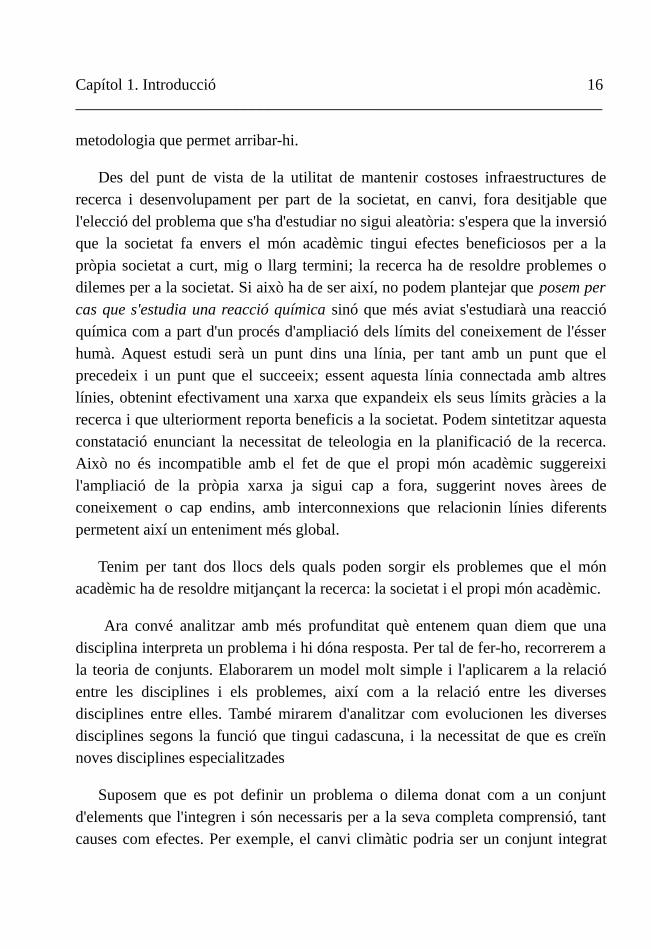
Què és doncs el que es conserva juntament amb l'arrel lingüística i que perdura com a interès per a l'home durant ja fa més de quatre mil anys? El que ha estat una constant durant tot aquest temps per a les persones que s'han dedicat a l'estudi de la χημία / al-kimia / química és l'interès per a comprendre la naturalesa de les transformacions en la matèria; un interès que ha transcendit fins i tot el fet de que el propi concepte de 'matèria' ha anat variant durant tots aquests mil·lennis, com és ben sabut. És a dir, el filòsof / alquimista / químic ha mantingut interès per les transformacions de la matèria sigui aquesta una manifestació de quelcom que
Figura 1.1. Imatge d'un tractat sobre alquímia escrit per Ramon Llull.
Capítol 1. Introducció 4__________________________________________________________________
transcendeix el món més cognoscible, sigui un ens continu, sigui un ens divisible en entitats discretes; la naturalesa de la matèria és únicament necessàri entendre-la com a subjecte del canvi per a poder articular una disciplina com la que ens ocupa i donar-li una continuïtat mil·lenària.
La química que vàrem heretar de Lavoisier ens és ja molt propera. En una Europa il·lustrada de la mà de personatges com Kant, Newton, Leibniz, Voltaire, Lagrange, Euler i D'Alembert la matematització de la física porta aquesta disciplina germana a enlluernar el món amb un poder de predicció i un rigor que fan considerar obsoleta la manera d'abordar el coneixement practicada amb anterioritat. L'èxit aviat va traslladar-se a la química, per la via de sistematitzar la química de la mateixa manera que s'havia sistematitzat la física, tot i que no va ser immediat (Newton encara practicava l'alquímia). El fet de que totes dues disciplines ara beguessin de les mateixes aigües en el seu camí cap a la consolidació en una nova era d'èxit tecnològic i prestigi fa que sigui previsible que avui haguem acabat parlant de físicoquímica o química física en moltes ocasions; en molts casos tenim problemes que es poden abordar des de la química o des de la física, i el fet de que ambdues es reconeguin en els mateixos paradigmes gràcies a la nova aproximació a la ciència que neix de la Il·lustració afavoreix la creació d'àrees interdisciplinàries.
Aquesta nova mirada sobre el problema químic per excel·lència des d'una òptica físicoquímica ens proporciona ja una nova manera d'acostar-nos al canvi químic i que anirà madurant en els segles posteriors: es tractarà de la comprensió primer de la naturalesa de la fenomenologia microscòpica a nivell atòmic i molecular; i després la inferència partir d'aquest coneixement de com ha de ser el canvi a nivell macroscòpic. D'aquí sorgirà el que anomenarem química teòrica (i també la física molecular).
Pocs anys després de la publicació de l'equació de Schrödinger (1926), naixerà el mètode Hartree – Fock (1935) utilitzat encara avui dia com a primera aproximació dins la química teòrica; de manera que veiem com de nou un avenç en el camp de la física (la mecànica quàntica) es tradueix en una nova manera d'enfocar problemes químics, engendrant una disciplina quimicofísica com és la

De la superfície d'energia potencial a la reactivitat química 5__________________________________________________________________
química teòrica. Ràpidament van sorgir dues maneres noves d'entendre àtoms i molècules: la teoria d'enllaç valència (en anglès Valence Bond, VB) creada i/o desenvolupada per Slater, Pauling, Van Vleck, Heitler, London i Eyring (anomenada, de fet, inicialment, Heitler-London-Slater-Pauling, HLSP); i la teoria d'orbitals moleculars (en anglès Molecular Orbitals, MO) creada i/o desenvolupada per Hund, Mulliken, Hückel, Coulson, Lennard-Jones i Slater. També resta la vessant més estadística basada en teories de Maxwell i Boltzmann, així com la interpretació basada en la mecànica clàssica; ambdues molt utilitzades en dinàmica encara avui dia.
A continuació s'ofereix un breu resum d'alguns dels moments més destacats en el desenvolupament de les bases de la química teòrica durant el segle XX.[1], [2], [3], [4],
[5], [6], [7]
Any Estructura electrònica Dinàmica
1916-1920
Lewis proposa el seu model estructural.
Teoria de la col·lisió en fase gas, Lewis, Herzfeld, Polanyi (I més tard (1937) Hinshelwood)
1925 Primera publicació de Heisenberg sobre mecànica quàntica
1926 Equació de SchrödingerCamp Autoconsistent (SCF), HartreeTeoria d'Enllaç València
Schrödinger utilitza el concepte de paquet d'ones per connectar la mecànica clàssica i la quàntica.
1927 Aproximació Born-OppenheimerModel de Thomas - Fermi
1928 Concepte de ressonància, Pauling
1929 Combinació Lineal d'Orbitals Atòmics (LCAO), Lennard –
Capítol 1. Introducció 6__________________________________________________________________
JonesDeterminants en el tractament de la funció d'ona, Slater
1930 Concepte d'hibiridació, Pauling
Teoria d'Orbitals Moleculars
Teoria del Camp Cristal·lí (Crystal Field Theory), Bethe, Van Vleck
1931 Sistemes pi, Hückel S'estableixen les bases de la dinàmica quàntica, Wigner, Stone, Hahn i Hellinger
1934 Aplicació de la teoria de pertorbacions de Scrhödinger i Rayleigh sobre la funció d'ona (metodologia MP), MØller i Plesset
Dinàmica no adiabàtica (transicions Landau – Zener), Stueckelberg, Landau, i Zener
1935Teoria de l'estat de transició, Eyring, Evans i Polanyi; amb contribucions de Wigner i Marcelin.
1938 Publicació de “The Nature of the chemical bond”, PaulingPrimer càlcul acurat en la molècula d'hidrogen, Coulson
Finals 40
Representació de determinants de Slater com a combinació lineal de funcions gaussianes, BoysDewar publica el seu model de pertorbacions d'orbitals moleculars

De la superfície d'energia potencial a la reactivitat química 7__________________________________________________________________
1950 Pople millora l'aportació de Boys, establint el tipus de funcions de base utilitzades avui dia
1951 Combinació Lineal d'Orbitals Atòmics tal i com la coneixem avui, Roothan i Hall
1952 Coulson publica el llibre “Valence”
Teoria RRKM (Rice–Ramsperger–Kassel–Marcus), Marcus
1953 Diagrames de correlació, Walsh, Woodward, Hoffman
1954 Mètode UHF (originàriament DODS, Different Orbital for Different Spins), Pople, Nesbet, Berthier
Avenços importants en la consolidació fisicomatemàtica de la química quàntica, Löwdin, McWeeny, Roothan i Hall
Teoria coneguda en anglès com a Coupled Cluster (CC), Fritz Coester i Hermann Kümmel
1955 Primers càlculs ab initio per a un sistema gran, la molècula de nitrogen, Scherr
1960 Mètode ROHF, Roothan Teoria variacional de l'estat de transició, Keck. Truhlar la desenvoluparà.
1964 Teoremes de Hohenberg i Kohn

Capítol 1. Introducció 8__________________________________________________________________
1965 Model i equacions DFT de Kohn i Sham i aproximació local de la densitat (en anglès Local Density Aproximation, LDA) de Kohn i ShamMètode CNDO, Pople
1966 Jiři Čížek i Josef Paldus traslladen el mètode CC al càlcul de correlació electrònica en àtoms i molècules
1967 Primeres propagacions de paquets gaussians, Goldberg.
1968 Pulay publica derivades analítiques per a tota mena de funcionals
1969 Us de camps de força per optimitzar conformacions proteiques, Levitt i Liffson
1973 Neix el Protein Data BankPrimer càlcul d'interacció de configuracions multireferencial (en anglès, Multireference Configuration Interaction, MRCI), Liu. El mètode havia estat dissenyat per Peyerimhoff
'70s Separació de nivells (en anglès, Level Shift), Saunders, Hillier, Mitin
1975 Mètode de diagonalització de Davidson
1976 Mètode mecànica molecular /
De la superfície d'energia potencial a la reactivitat química 9__________________________________________________________________
mecànica quàntica (en anglès, molecular mechanics/ quantum mechanics, QM/MM) , Warshell i Levitt
1977 Primer estudi amb dinàmica molecular d'una proteïna, Karplus
1980 Mètode CASSCF, Roos. Basat en una contribució anterior de Ruedenberg (el FORS, Full Optimized Reaction Space, espai de reacció completament optimitzat)
Inversió directa de l'espai iteratiu (en anglès, Direct Inversion of the Iterative Space, DIIS), Pulay
1981 Neix el camp de força AMBER, Kollman
1982 Neix el docking, Kuntz
1986 Aproximació generalitzada del gradient al funcional de la densitat (en anglès Generalized Gradient Approximation, GGA), Perdew
1990 Mètode Hartree dependent del temps multiconfiguracional (en anglès Multiconfigurational Time Dependent Hartree, MCTDH), Meyer
Capítol 1. Introducció 10__________________________________________________________________
1993 Funcionals DFT híbrids, Becke
En aquesta breu descripció d'uns quants dels capítols més destacats sobre l'evolució de la química teòrica durant el segle XX s'han dividit els avenços en dues categories. Una correspon al tractament de la teoria electrònica en àtoms i molècules, les noves consideracions sobre l'energia i com es van consolidant mètodes diferents per tractar la correlació. La segona, anomenada dinàmica, tracta sobre teories d'origen estadístic i la integració d'equacions de moviment.
Al marge dels tipus i complexitat de les diferents aportacions que fan créixer la química teòrica (i cada cop més computacional) al llarg del segle XX podem adonar-nos d'un fet: a començaments de segle els noms i cognoms associats al desenvolupament de de tota la teoria (ja sigui estàtica o dinàmica) són sempre els mateixos. Això està molt en la línia del que havíem esmentat amb anterioritat: procedim de disciplines diferents que s'han reunit sota paradigmes idèntics i per tant hem passat de tenir especialistes en física per una banda, matemàtics per una altra i químics per una tercera a tenir científics que a través d'una base comuna poden comprendre i abastar moltes disciplines. La tendència a finals de segle torna a ser la inversa tot i que no pels mateixos motius: una persona capdavantera d'un camp determinat sacrifica la seva capacitat de ser multidisciplinar per poder assolir un coneixement especialitzat en algun sector i així poder-lo fer avançar.
És immediat observar que això és una necessitat acadèmica: si un científic ha de fer avançar un camp determinat tot el temps que estigui formant-se en altres camps no serà productiu, en principi, per tal de dur a terme aquesta tasca. No obstant, aquest fet té diverses contrapartides: per exemple, no serà capaç d'importar metodologies d'altres camps que podrien ser útils en el seu propi camp; però per altra tenim una conseqüència que crida molt l'atenció: a l'hora d'afrontar un problema físic, la resposta vindrà donada per una metodologia que alhora dependrà de la formació i trajectòria de la persona que vulgui resoldre el problema. Caldria esperar que la resposta fora sempre la mateixa: hem estat parlant de diferents disciplines que han confluït en uns paradigmes fisicomatemàtics que les

De la superfície d'energia potencial a la reactivitat química 11__________________________________________________________________
unifiquen totes. No obstant, una ullada a la literatura ens permet adonar-nos que diferents disciplines aporten una mirada diferent sobre un mateix problema; i aquest problema es considera 'resolt' un cop les eines metodològiques corresponents a cada disciplina hi han estat aplicades. Tenim diverses respostes i totes són vàlides en el sentit de que són legítimament considerades com a vàlides per diferents disciplines.
Posem per cas que s'estudia una donada reacció química. Analitzem les diferents aproximacions que poden fer tres persones diferents a aquesta reacció, entenent com a aproximació la mena d'estudi que durà a terme i mirarà de publicar. Una persona especialitzada en estructura i correlació electrònica donarà per resolt el problema oferint com a resposta la caracterització de reactius, productes i estats de transició a un nivell de càlcul i teoria que consideri adients. Una persona especialitzada en modelització i dinàmica quàntica resoldrà el mateix problema oferint un model simplificat que sigui representatiu de la reacció i a continuació
Figura 1.2. Alguns dels protagonistes del món acadèmic de començaments del segle XX apareguts a la taula precedent.
Capítol 1. Introducció 12__________________________________________________________________
donant dades sobre la reactivitat del sistema de dimensionalitat reduïda, per exemple un diagrama de probabilitat en funció de l'energia. Una persona especialitzada en dinàmica clàssica podria presentar unes seccions eficaces calculades fent estadística d'una sèrie de trajectòries, suficients com per a ser estadísticament significatives; o bé una aproximació a la constant de velocitat. Són tres respostes molt vàlides i possiblement serien acceptades sense problemes per la comunitat i publicades.
Veiem doncs com la química teòrica i computacional ha après a donar respostes molt complertes; fins i tot s'ha ramificat fins a tal punt que és capaç de donar respostes diferents, ja que n'han sorgit disciplines diferents. D'aquestes respostes hom n'espera una sèrie de característiques, en relació les unes amb les altres.
La més important és que no siguin contradictòries. Això ve assegurat pel fet de que totes les àrees dins la química teòrica tenen les mateixes arrels teòriques, tant físiques com matemàtiques. Fins i tot encara que en l'exemple anterior una dinàmica clàssica i una de quàntica donin resultats qualitativament diferents, aquesta diferència s'accepta com a normal pel fet de que la mecànica quàntica dóna informació que la clàssica no pot donar degut a que és un model diferent i que descriu de manera incompleta els sistemes microscòpics. També podem obtenir respostes diferents segons el grau d'aproximació que emprem per tal de fer possible un càlcul, per exemple a l'hora de decidir com de gran és la base mitjançant la qual propagarem un paquet d'ones o fins a quin nombre de dimensions reduirem el nostre problema. Aquestes respostes diferents simplement indicarien que s'ha escapçat massa el càlcul, produint resultats que no són representatius; tampoc és el cas que ens ocupa. El que ens ocupa és mirar d'esbrinar per què caracteritzar acceptablement un sistema químic no és quelcom unívoc.
Una altra característica tracta sobre quina mena de relació tenen a part de la no contradicció. Són complementàries? Són interpretacions d'un mateix sistema físic totalment independents? Per exemple, tornant a la dinàmica clàssica i la quàntica: No té sentit mirar de comparar una funció de probabilitat en funció de l'energia amb els resultats clàssics; en física clàssica la probabilitat només és zero o u. No

De la superfície d'energia potencial a la reactivitat química 13__________________________________________________________________
obstant la superfície d'energia potencial obtinguda a través de l'estructura electrònica més que complementària és essencial per tal de poder fer una o l'altra dinàmica.
Per esclarir aquesta qüestió val la pena mirar d'aprofundir en les respostes que dóna cada visió. Ens centrarem en la química molecular.
III. Aportacions de l'estructura electrònica
S'han escrit moltes reflexions sobre les aportacions de l'estructura electrònica. Si prenem com a exemple concret aquest compendi d'un autor experimentat[8]
veiem que a mitjans dels noranta es destaquen dues vessants de l'estructura electrònica en quant a la seva capacitat de predicció (aquesta separació no neix en aquest compendi): per una banda la d'estructures d'equilibri, verificables mitjançant espectroscòpia, i per l'altra la de diferències energètiques (entalpies, barreres de reacció, canvi de conformació, dissociació...). També es parla de moments dipolars i espectres d'infraroig.
A més d'això, també es poden predir nombrosos espectres: RMN[9], UV i d'altres que queden més lluny de la química convencional com poden ser els Auger[10].
Més enllà de la predicció d'estructures que hom pot associar a punts estacionaris dins una superfície d'energia potencial, la teoria de camins de reacció[11] permet explorar corbes sobre la superfície que poden arribar a donar una idea aproximada sobre l'evolució d'una reacció química. [12]
En el camp dels mètodes semiempírics en el context dels camps de força s'ha pogut arribar al càlcul d'energia de les macromolècules. Fins, per a part del sistema, s'incorpora metodologia quàntica (metodologia QM/MM)[7].
Capítol 1. Introducció 14__________________________________________________________________
IV. Aportacions de la dinàmica
Si emprem models com el RRKM per predir el comportament d'un sistema, parlem de dinàmica teòrica. Aquesta dinàmica, arrelada fortament a la física estadística de Maxwell i Boltzmann i que arrenca amb l'equació d'Arrhenius, connecta el coneixement teòric d'un sistema químic amb la vessant més cinètica de l'experiment. La informació que n'extraurem seran constants de velocitat; però també temps de vida de molècules, distribució d'energia dins una molècula o la reactivitat de canals reactius. Aquesta vessant de la dinàmica s'ha fet moltes vegades imprescindible per tal de poder interpretar experiments.[13]
Quan integrem equacions de moviment (clàssiques o quàntiques) i en seguim l'evolució sobre una superfície d'energia potencial seguim dins el camp de la dinàmica però hom es refereix a aquesta vessant com a computacional. Fent això, obtenim la visió més profunda sobre la reactivitat que la química teòrica pot oferir donat que seguim les molècules una a una en el seu trànsit per la superfície d'energia potencial. Podem acumular trajectòries clàssiques per tal de fer estadístiques que ens apropin a resultats experimentals pel que fa a constants de velocitat, transferència intramolecular o extramolecular d'energia o seccions eficaces. El baix cost computacional d'aquestes trajectòries ens permet abastar també el camp de la dinàmica de macromolècules, incorporant fins i tot dissolvent. Utilitzant les aproximacions pertinents també podem utilitzar trajectòries clàssiques per tal d'estudiar dinàmiques no adiabàtiques. Si les trajectòries són quàntiques, obtenim directament la magnitud d'efectes propis d'aquest model com poden ser l'efecte túnel o ressonàncies. Entrant en el paradigma quàntic, també tenim dinàmiques electròniques per tal de comprendre els bescanvis d'energia entre diferents estats d'una molècula involucrada en processos d'emissió o absorció d'energia; així mateix, és vital per tal d'entendre la femtoquímica.[14]
V. Preguntes i respostes: societat i món acadèmic
Ens trobem davant de dues maneres d'enfocar la química teòrica. Responent a
De la superfície d'energia potencial a la reactivitat química 15__________________________________________________________________
la pregunta plantejada amb anterioritat, la informació que ofereix cada aproximació és més complementària que no pas excloent. En alguns casos, una informació dinàmica pot resultar redundant respecte al que aporta ja l'estructura electrònica. D'altres, pot aportar informació addicional. Aquesta informació de més pot tenir rellevància o no.
Hem estat parlant durant les seccions que precedeixen aquesta sobre “respostes”. Hom entén que el paper d'una disciplina com la química teòrica i qualsevol de les disciplines que aquesta engloba és oferir precisament això, respostes. Després de reflexionar un instant sobre la mena de resposta que podem obtenir es fa cada cop més imminent començar-nos a preguntar pel que realment és el quid de la qüestió: davant de tanta resposta, quina era la pregunta?
Expressament, durant la discussió anterior s'ha plantejat la qüestió posem per cas que s'estudia una reacció química de manera que esquivéssim aquest dilema fonamental fins arribar a aquest punt. Plantejar una discussió sobre quina disciplina ha d'afrontar l'estudi d'una reacció química donada analitzant la mena de respostes que poden donar les diverses aproximacions que podem emprar per a fer-ho és impossible: ja hem dit que des del punt de vista fonamental tots són vàlids i no es poden contradir; i també hem constatat que des del punt de vista de les aplicacions de cadascun i fent un brevíssim cop d'ull a la bibliografia la informació que aporta cadascun no és excloent envers la informació que aporten els altres. Així doncs la reflexió sobre quina és la millor disciplina per tal d'estudiar una reacció química concreta ha de raure en la reacció química en sí. Es coneixen moltes reaccions químiques: algunes han estat estudiades exhaustivament; d'altres només parcialment; algunes no han estat estudiades, potser perquè encara no es coneixen. Triar una reacció química a l'atzar d'entre aquestes tres categories i realitzar un estudi donat dins d'alguna de les disciplines que s'han esmentat i descrit anteriorment és el que implica l'enunciat posem per cas que s'estudia una reacció química. Des del punt de vista acadèmic això no és extravagant. Quan hom publica un article, s'inclou un apartat d'introducció que inclou contextualització, precedents i objectius; però sovint aquesta no és la part que més atrau l'atenció del lector que com a especialista busca directament les conclusions o la formulació o
Capítol 1. Introducció 16__________________________________________________________________
metodologia que permet arribar-hi.
Des del punt de vista de la utilitat de mantenir costoses infraestructures de recerca i desenvolupament per part de la societat, en canvi, fora desitjable que l'elecció del problema que s'ha d'estudiar no sigui aleatòria: s'espera que la inversió que la societat fa envers el món acadèmic tingui efectes beneficiosos per a la pròpia societat a curt, mig o llarg termini; la recerca ha de resoldre problemes o dilemes per a la societat. Si això ha de ser així, no podem plantejar que posem per cas que s'estudia una reacció química sinó que més aviat s'estudiarà una reacció química com a part d'un procés d'ampliació dels límits del coneixement de l'ésser humà. Aquest estudi serà un punt dins una línia, per tant amb un punt que el precedeix i un punt que el succeeix; essent aquesta línia connectada amb altres línies, obtenint efectivament una xarxa que expandeix els seus límits gràcies a la recerca i que ulteriorment reporta beneficis a la societat. Podem sintetitzar aquesta constatació enunciant la necessitat de teleologia en la planificació de la recerca. Això no és incompatible amb el fet de que el propi món acadèmic suggereixi l'ampliació de la pròpia xarxa ja sigui cap a fora, suggerint noves àrees de coneixement o cap endins, amb interconnexions que relacionin línies diferents permetent així un enteniment més global.
Tenim per tant dos llocs dels quals poden sorgir els problemes que el món acadèmic ha de resoldre mitjançant la recerca: la societat i el propi món acadèmic.
Ara convé analitzar amb més profunditat què entenem quan diem que una disciplina interpreta un problema i hi dóna resposta. Per tal de fer-ho, recorrerem a la teoria de conjunts. Elaborarem un model molt simple i l'aplicarem a la relació entre les disciplines i els problemes, així com a la relació entre les diverses disciplines entre elles. També mirarem d'analitzar com evolucionen les diverses disciplines segons la funció que tingui cadascuna, i la necessitat de que es creïn noves disciplines especialitzades
Suposem que es pot definir un problema o dilema donat com a un conjunt d'elements que l'integren i són necessaris per a la seva completa comprensió, tant causes com efectes. Per exemple, el canvi climàtic podria ser un conjunt integrat

De la superfície d'energia potencial a la reactivitat química 17__________________________________________________________________
per elements com la pèrdua d'ozó, l'increment del diòxid de carboni o la migració d'espècies animals. Anomenarem aquests conjunts 'Prob'.
Utilitzem disciplines per entendre aquesta problemàtica. Suposem que una disciplina donada es pot definir com el conjunt d'elements que aquesta disciplina és capaç de reconèixer com a propis. Per exemple, la química podria constar de la descomposició de l'ozó o l'oxidació d'un metall, però no la migració d'espècies animals. Anomenarem aquests conjunts 'Disc'
Per tal de copsar totalment una problemàtica, una disciplina ha de contenir tots els elements que la caracteritzen. En teoria de conjunts, això equival a dir que la problemàtica haurà de ser un subconjunt dins el conjunt disciplina; això es pot expressar dient que la intersecció entre la disciplina i la problemàtica hauran de ser iguals a la problemàtica de nou.
Figura 1.3. Es mostra una síntesi del que s'ha esmentat als darrers paràgrafs. El món acadèmic ha de resoldre problemes plantejats des de la societat o proposats per ell mateix. A través de disciplines diferents es fan interpretacions diferents. Són compatibles perquè passen a travès d'un mateix paradigma fisicomatemàtic. Cada interpretació condueix a una solució diferent. I la solució torna per reacaure a la societat.
Disciplina 1
Disciplina 2
Disciplina n
Interpretació 1
Interpretació 2
Interpretació n
Fonamentsfisicomatemàtics
Solució 1
Solució 2
Solució n
Problema -
Dilema
Món acadèmic
Societat
Capítol 1. Introducció 18__________________________________________________________________
Disc∩Prob=Prob
En aquest model això equivaldria a dir que la problemàtica està resolta en el marc d'aquella disciplina.
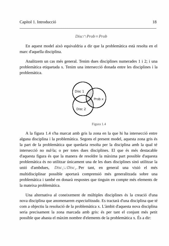
Analitzem un cas més general. Tenim dues disciplines numerades 1 i 2; i una problemàtica etiquetada x. Tenim una intersecció donada entre les disciplines i la problemàtica.
A la figura 1.4 s'ha marcat amb gris la zona en la que hi ha intersecció entre alguna disciplina i la problemàtica. Segons el present model, aquesta zona gris és la part de la problemàtica que quedaria resolta per la disciplina amb la qual té intersecció no nul·la; o per totes dues disciplines. El que és més destacable d'aquesta figura és que la manera de resoldre la màxima part possible d'aquesta problemàtica és no utilitzar únicament una de les dues disciplines sinó utilitzar la
unió d'ambdues, Disc1∪Disc2. Per tant, en general una visió el més
multidisciplinar possible aportarà comprensió més generalitzada sobre una problemàtica i també en donarà respostes que tinguin en compte més elements de la mateixa problemàtica.
Una alternativa al coneixement de múltiples disciplines és la creació d'una nova disciplina que anomenarem especialitzada. Es tractarà d'una disciplina que té com a objectiu la resolució de la problemàtica x. L'àmbit d'aquesta nova disciplina seria precisament la zona marcada amb gris: és per tant el conjunt més petit possible que abasta el màxim nombre d'elements de la problemàtica x. És a dir:
Figura 1.4
De la superfície d'energia potencial a la reactivitat química 19__________________________________________________________________
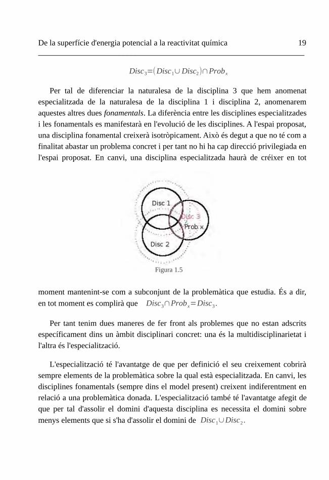
Disc3=(Disc1∪Disc2)∩Probx
Per tal de diferenciar la naturalesa de la disciplina 3 que hem anomenat especialitzada de la naturalesa de la disciplina 1 i disciplina 2, anomenarem aquestes altres dues fonamentals. La diferència entre les disciplines especialitzades i les fonamentals es manifestarà en l'evolució de les disciplines. A l'espai proposat, una disciplina fonamental creixerà isotròpicament. Això és degut a que no té com a finalitat abastar un problema concret i per tant no hi ha cap direcció privilegiada en l'espai proposat. En canvi, una disciplina especialitzada haurà de créixer en tot
moment mantenint-se com a subconjunt de la problemàtica que estudia. És a dir,
en tot moment es complirà que Disc3∩Probx=Disc3.
Per tant tenim dues maneres de fer front als problemes que no estan adscrits específicament dins un àmbit disciplinari concret: una és la multidisciplinarietat i l'altra és l'especialització.
L'especialització té l'avantatge de que per definició el seu creixement cobrirà sempre elements de la problemàtica sobre la qual està especialitzada. En canvi, les disciplines fonamentals (sempre dins el model present) creixent indiferentment en relació a una problemàtica donada. L'especialització també té l'avantatge afegit de que per tal d'assolir el domini d'aquesta disciplina es necessita el domini sobre
menys elements que si s'ha d'assolir el domini de Disc1∪Disc2.
Figura 1.5

Capítol 1. Introducció 20__________________________________________________________________
S'ha mencionat anteriorment d'on poden sorgir noves problemàtiques. Es suggereixen dos tipus de nova problemàtica que pot sorgir dins el model sota estudi. Un tipus és la nova problemàtica que sorgeix durant l'estudi d'una problemàtica ja coneguda, és a dir, sorgeix durant l'examen d'algun element o alguns elements de la problemàtica que s'estudiava i que formen part de Proby∩Probx . Així la nova problemàtica y compleix:
Proby∩Probx≠{∅}
Ja que per imposició la disciplina 3 no pot abastar elements fora de la problemàtica x, tot i que aquesta ha estat probablement pionera a l'hora de descobrir els elements que han endegat l'estudi de la problemàtica y, aquesta no podrà estudiar elements de la problemàtica y que no estiguin en x:
Disc3∩(Prob y−Probx)={∅}
Com a comentari addicional, no seria estrany que a partir de la disciplina 3 en sorgís una de nova per tal d'encetar la investigació de la problemàtica y, potser conjuntament amb alguna altra disciplina que també tingui elements en comú amb la nova problemàtica y. Però no aprofundirem més en aquest sentit.
Una situació oposada, és que la nova problemàtica no tingui elements en comú amb la problemàtica x. Això representaria una nova problemàtica que no apareix
Figura 1.6

De la superfície d'energia potencial a la reactivitat química 21__________________________________________________________________
durant la investigació d'una problemàtica coneguda com en el cas anterior sinó que ve des de fora: a la figura 3 equivaldria a que la societat proposi un problema nou al món acadèmic.
Ja que s'ha imposat que la nova problemàtica z no comparteix elements amb la problemàtica x, la disciplina 3 no pot estudiar-la en cap cas:
Probz∩Probx=Probz∩Disc3={∅}
Per tant, ha de ser a través d'altres disciplines que es tracti aquest problema. Les disciplines especialitzades hauran crescut per tal de solucionar reptes concrets, de manera un repte nou d'un àmbit diferent els serà desconegut. No obstant, les disciplines fonamentals han crescut en totes les direccions i estan més capacitades per reconèixer elements de noves problemàtiques.
VI. Conclusions
Les conclusions més rellevants d'aquest capítol han estat les següents:
– Durant el segle XX les disciplines teòriques que envolten la química s'observa l'aparició de moltes disciplines especialitzades.
– Aquestes disciplines resolen problemes amb interpretacions diferents i poden donar solucions diferents. Però no són contradictòries.
Figura 1.7

Capítol 1. Introducció 22__________________________________________________________________
– És important la reflexió sobre l'impacte de la recerca a la societat i que la planificació de la mateixa obeeixi una certa teleologia.
Segons el model proposat:
– La multidisciplinarietat i l'especialització són respostes vàlides a l'hora d'abastar nous problemes. La creació de disciplines especialitzades és la manera més òptima d'abastar el problema sobre el que s'especialitza.
– Les disciplines fonamentals permeten analitzar problemes nous gràcies a la seva generalitat.
Tornant als dilemes plantejats a la secció I, es constata que totes les aportacions donades des de diferents disciplines especialitzades (l'estructura electrònica, la dinàmica (clàssica i quàntica) i la teoria de camins de reacció) són vàlides i s'ha de buscar la complementarietat entre elles. L'anàlisi de la informació que aportarà cadascuna no es pot deslligar dels problemes concrets que han de tractar; i el problema té més a dir sobre quines eines utilitzar en cada cas que no pas la disponibilitat d'aquestes eines o dels mitjans per utilitzar-les. És de vital importància tenir sempre una base ferma en disciplines fonamentals (química, física, matemàtiques, etc.) ja que donen una perspectiva crucial per tal d'entendre nous problemes (o vells problemes amb els que un determinat individu no està familiaritzat).
Bibliografia
1. E . B. Wilson, Pure & Applied Chemistry, 47, 41-47 (1976)
2. S . G. Christov. Collision Theory and Statistical Theory of Chemical Reactions. Springer-Verlag (1980)
3. P . G. Szalay, T. Müller, G. Gidofalvi, H. Lischka i R. Shepard, Chemical Reviews, 112, 108-181 (2012)
4. K. Burke, The Journal of Chemical Physics, 136, 150901 (2012)
De la superfície d'energia potencial a la reactivitat química 23__________________________________________________________________
5. D . G. Truhlar i B. C. Garrett, Annual Review of Physical Chemistry, 35, 159-189 (1984)
6. B . M. Garraway i K. -. Suominen, Reports on Progress in Physics, 58, 365 (1995)
7. A. Warshel i M. Levitt, Journal of Molecular Biology, 103, 227 - 249 (1976)
8. H . F. Schaefer III, J. R. Thomas, Y. Yamaguchi, B. J. Deleeuw i G. Vacek. The Chemical Applicability Of Standard Methods In Ab Initio Molecular Quantum Mechanics. A Modern Electronic Structure Theory Part I. David R. Yarkony (Ed.), (1995) 3-54.
9. T. Helgaker, M. Jaszunski i K. Ruud, Chemical Reviews-Columbus, 99, 293 (1999)
10. B. Schimmelpfennig i S. Peyerimhoff, Chemical Physics Letters, 253, 377 - 382 (1996)
11. H . B. Schlegel, WIREs Computational Molecular Science, 1, 790-809 (2011)
12. J . M. Bofill, W. Quapp i M. Caballero, Journal of Chemical Theory and Computation, 8, 927-935 (2012)
13. U. Lourderaj i W. L. Hase, The Journal of Physical Chemistry A, 113, 2236-2253 (2009)
14. A . H. Zewail, The Journal of Physical Chemistry A, 104, 5660-5694 (2000)

Capítol 2
Als mateixos rius entrem i no entrem, [car] som i no som [els mateixos].
Heràclit d'Efes – segles V - IV a.C.
Estructura electrònica

De la superfície d'energia potencial a la reactivitat química 25 __________________________________________________________________
I. L'equació de Schrödinger
Actualment, l'equació de Schrödinger i algunes de les maneres de trobar-ne una solució aproximada són discutides en desenes de textos considerats bàsics per qualsevol estudiant de química teòrica. Un exemple pel que fa als mètodes anomenats 'de funció d'ona' són les referències 1 i 2.
Hi ha una gran acceptació de que la manera de conèixer amb més profunditat les propietats d'un sistema microscòpic tal i com és un sistema molecular és resoldre l'equació de Schrödinger. Hom sol parlar de dues variants d'aquesta equació: la dependent del temps i la independent del temps. Pel que fa a la predicció d'estructures i camins de reacció, l'opció escollida sol ser l'equació independent del temps; donat que els nuclis no es mouen en el temps, és comú relacionar aquesta solució amb el terme 'estàtic'a en contraposició a la 'dinàmica' que aportaria el component temporal. Aquesta equació es pot escriure de la següent forma:
H Ψ=EΨ (2.1)
on H és un operador matricial i hermíticb anomenat hamiltonià. La funció pròpia Ψ es coneix com a funció d'ona. Una possible deducció d'aquesta equació és la
que s'inclou a l'apèndix B.
Als llibres de text l'estructura de l'hamiltonià com a operador sol ser similar a aquesta:
H tot=Tn+T e+Vne+Vee+Vnn (2.2)
a Aquesta nomenclatura de vegades també es fa servir per parlar de tipus de correlació en un context diferent. Aleshores es parla de la correlació estàtica per referir-se a la correlació forta i de la dinàmica per referir-se a la correlació feble.
b Una matriu hermítica és aquella matriu que és quadrada, complexa i és autoadjunta. Una de les seves propietats més interessants és que tota matriu hermítica és diagonalitzable per una matriu unitària; els seus valors propis seran tots reals i formen un conjunt que es pot escollir ortonormal.

Capítol 2. Estructura electrònica 26 __________________________________________________________________
Aquí, T fa referència a l'energia cinètica i V fa referència a l'energia potencial. Els subíndex n fan referència als nuclis i els e, als electrons. Els operadors que incorporen dos subíndex fan referència a interaccions entre partícules.
Reagruparem termes anomenant He a la suma de T e+Vne+Vee+V nn , de
manera que H tot=He+Tn . D'aquesta manera aconseguim un hamiltonià ( He ) que
depèn de les posicions dels nuclis però no dels seus moments. La solució a l'equació de Schrödinger per a aquest hamiltonià tindria la següent forma:
He (R )ψi(R , r)=Ei(R)ψi(R ,r) i=1,2 ,...∞ (2.3)
En aquest punt és rellevant recordar que, ja que el hamiltonià és hermític, les seves solucions poden ser escollides com a base ortonormal, de manera que es satisfà una relació amb aquesta forma:
∫ψi*(R ,r) ψj(R ,r )dr=δij (2.4)
on apareix la delta de Kronecker que pren els valors
δij=1, i= jδij=0, i≠ j
Sense introduir cap mena d'aproximació, la funció d'ona exacta pot ser expressada mitjançant una expansió de funcions electròniques amb uns coeficients que podem escollir que siguin funció de les coordenades nuclears:
Ψ(R , r)=∑i=1
∞
ψn i(R)ψi(R , r) (2.5)
Amb aquestes consideracions, l'equació de Schrödinger es pot reescriure així:
∑i=1
∞
(Tn+He)ψn i(R)ψi(R , r )=Etot∑i=1
∞
ψn i(R) ψi(R , r) (2.6)
De cara al següent desenvolupament, és convenient considerar que Tn és un
De la superfície d'energia potencial a la reactivitat química 27 __________________________________________________________________
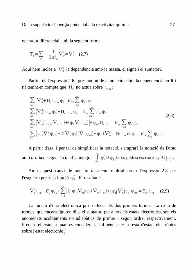
operador diferencial amb la següent forma:
Tn=∑a
−1
2M a
∇ a2=∇n
2 (2.7)
Aquí hem inclós a ∇n2 la dependència amb la massa, el signe i el sumatori.
Partint de l'expressió 2.6 i prescindint de la notació sobre la dependència en R i
r i tenint en compte que He no actua sobre ψn i :
∑i=1
∞
(∇ n2+He)ψn iψi=E tot∑
i=1
∞
ψn i ψi
∑i=1
∞
{∇ n2(ψn i ψi)+Heψn i ψi }=E tot∑
i=1
∞
ψn iψi
∑i=1
∞
{∇ n [(ψn i ∇n ψi)+(ψi ∇n ψn i) ]+ψn i Heψi }=Etot∑i=1
∞
ψn iψi
∑i=1
∞
{ψi(∇ n2ψn i)+2(∇ nψi)(∇ n ψn i)+ψn i(∇ n
2ψi)+ψn i Ei ψi }=Etot∑
i=1
∞
ψn iψi
(2.8)
A partir d'ara, i per tal de simplificar la notació, s'emprarà la notació de Dirac
amb bra-ket, segons la qual la integral ∫−∞
∞
ψi* Oψ j dr es podria escriure ⟨ψi∣O∣ψj ⟩ .
Amb aquest canvi de notació in mente multiplicarem l'expressió 2.8 per
l'esquerra per una funció ψ j* . El resultat és:
∇n2ψn j+E jψn j+∑
i=1
∞
{2 ⟨ψ j∣∇ n∣ψi ⟩ (∇ nψn i)+⟨ψ j∣∇ n2∣ψi ⟩ψn i }=E totψn j (2.9)
La funció d'ona electrònica ja no afecta els dos primers termes. La resta de termes, que encara figuren dins el sumatori per a tots els estats electrònics, són els anomenats acoblaments no adiabàtics de primer i segon ordre, respectivament. Prenen rellevància quan es considera la influència de la resta d'estats electrònics sobre l'estat electrònic j.

Capítol 2. Estructura electrònica 28 __________________________________________________________________
En l'anomenada aproximació adiabàtica es negligeixen totes les integrals que involucren diferents estats. Per altra banda, és conegut que l'acoblament adiabàtic
de primer ordre {ψi∣∇n∣ψi } és sempre nul si la funció d'ona no és degenerada en la
seva component espacial. Amb aquestes consideracions, l'equació 2.9 queda reduïda a:
(∇n2+E j+ ⟨ψ j∣∇ n
2∣ψ j ⟩ )ψn j=Etot ψn j (2.10)
que podem reescriure per tal de visualitzar amb més claredat el que implica de la següent manera:
(Tn+E j(R)+U (R))ψn j(R )=Etotψn j(R) (2.11)
Aquí apareix un nou terme, U(R), que engloba l'acoblament adiabàtic de segon ordre i és conegut com a correcció diagonal. Usualment trobem que aquest terme
varia molt lentament en funció de R i és, en relació a E j , de baixa magnitud:
aproximadament la proporció ve donada per la suma de les masses dels nuclis (equació 2.7); en conseqüència es sol negligir sota el que s'anomena aproximació
Born-Oppenheimer. Això permet prendre l'energia electrònica E j com si fos una
energia potencial:
(Tn+E j(R ))ψn j (R)=(Tn+V j(R))ψn j(R)=E totψn j(R) (2.12)
Amb l'acceptació d'aquestes aproximacions neix la imatge de que els nuclis es mouen en una hipersuperfície d'energia potencial que és una solució de l'equació electrònica de Schrödinger. La superfície no és sensible a un canvi en les masses i per tant no hi ha efectes isotòpics. Aquesta superfície d'energia potencial que satisfà a la vegada l'aproximació adiabàtica i la de Born-Oppenheimer és el concepte fonamental en el si del qual es desenvolupa tota la teoria de camins de reacció que examinarem al capítol 3.
A les seccions següents es durà a terme un recull esquemàtic d'estratègies per a la resolució de l'equació de Schrödinger.
De la superfície d'energia potencial a la reactivitat química 29 __________________________________________________________________
II. Solucions a l'equació de Schrödinger basades en la funció d'ona
No es coneixen solucions exactes de l'equació de Schrödinger tal i com està plantejada a l'apartat anterior per a la majoria de sistemes d'interès químic. De fet,
només es poden resoldre de forma exacta l'àtom d'hidrogen, la molècula H2+ i
altres sistemes monoelectrònics similars. Això ja dóna una indicació força clara de quin és el principal problema en la resolució d'aquesta equació: com es tracta la manera en la que el moviment d'un electró n'afecta al d'un altre - és l'anomenada correlació electrònica.
Totes les metodologies que es desenvolupen en aquesta secció són aproximacions de naturalesa ab initio; és a dir, en contrast als mètodes anomenats semiempírics, sense proporcionar informació sobre els sistemes a tractar en forma de parametrització.
II.1. Punt de partida: mètode Hartree – Fock
Els determinants de Slater
A la secció anterior s'ha tractat de manera formal la funció d'ona Ψ i s'ha
desenvolupat com a combinació lineal d'altres funcions, {ψi } . Finalment, hem
plantejat la solució de l'equació de Schrödinger en termes d'aquest segon conjunt
de funcions {ψi } ; concretament unes que depenen només de les coordenades
nuclears. No obstant, no s'ha dit res sobre l'estructura d'aquesta mena de funcions.
Aquestes funcions han de tenir una part espacial que depengui certament de les coordenades nuclears però també han de tenir un component de espín. Degut a que el nostre hamiltonià és no relativista no tenim més remei que incloure aquest component d'espín ad hoc. A més, l'electró és de naturalesa fermiònica i, per tant,
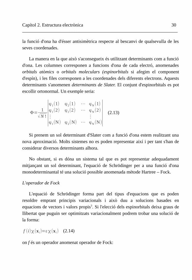
Capítol 2. Estructura electrònica 30 __________________________________________________________________
la funció d'ona ha d'ésser antisimètrica respecte al bescanvi de qualsevulla de les seves coordenades.
La manera en la que això s'aconsegueix és utilitzant determinants com a funció d'ona. Les columnes corresponen a funcions d'ona de cada electró, anomenades orbitals atòmics o orbitals moleculars (espinorbitals si afegim el component d'espín), i les files corresponen a les coordenades dels diferents electrons. Aquests determinants s'anomenen determinants de Slater. El conjunt d'espinorbitals es pot escollir ortonormal. Un exemple seria:
Φ= 1√N ! ∣
ϕ1(1) ϕ2(1) ⋯ ϕN (1)ϕ1(2) ϕ2(2) ⋯ ϕN (2)⋮ ⋮ϕ1(N) ϕ2(N) ⋯ ϕN (N)
∣ (2.13)
Si prenem un sol determinant d'Slater com a funció d'ona estem realitzant una nova aproximació. Molts sistemes no es poden representar així i per tant s'han de considerar diversos determinants alhora.
No obstant, si es dóna un sistema tal que es pot representar adequadament mitjançant un sol determinant, l'equació de Schrödinger per a una funció d'ona monodeterminantal té una solució possible anomenada mètode Hartree – Fock.
L'operador de Fock
L'equació de Schrödinger forma part del tipus d'equacions que es poden resoldre emprant principis variacionals i això duu a solucions basades en equacions de vectors i valors propis3. Si l'elecció dels espinorbitals deixa graus de llibertat que puguin ser optimitzats variacionalment podrem trobar una solució de la forma:
f (i)χ (x i)=εχ (x i) (2.14)
on f és un operador anomenat operador de Fock:
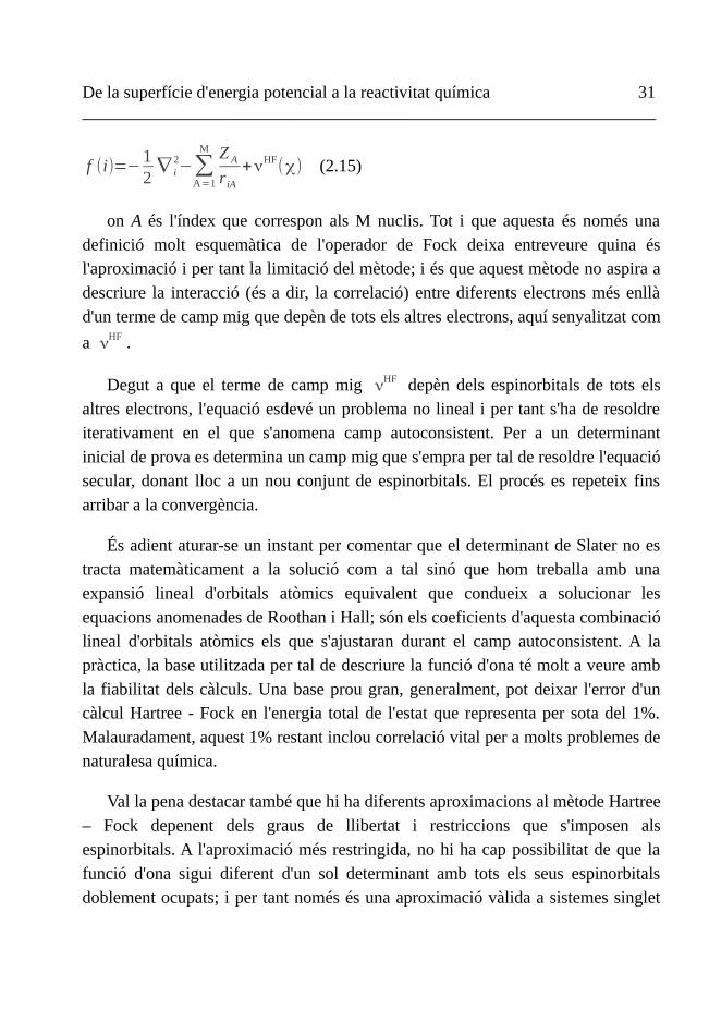
De la superfície d'energia potencial a la reactivitat química 31 __________________________________________________________________
f (i)=−12∇ i
2−∑A=1
M Z A
riA
+νHF(χ) (2.15)
on A és l'índex que correspon als M nuclis. Tot i que aquesta és només una definició molt esquemàtica de l'operador de Fock deixa entreveure quina és l'aproximació i per tant la limitació del mètode; i és que aquest mètode no aspira a descriure la interacció (és a dir, la correlació) entre diferents electrons més enllà d'un terme de camp mig que depèn de tots els altres electrons, aquí senyalitzat com
a νHF .
Degut a que el terme de camp mig νHF depèn dels espinorbitals de tots els altres electrons, l'equació esdevé un problema no lineal i per tant s'ha de resoldre iterativament en el que s'anomena camp autoconsistent. Per a un determinant inicial de prova es determina un camp mig que s'empra per tal de resoldre l'equació secular, donant lloc a un nou conjunt de espinorbitals. El procés es repeteix fins arribar a la convergència.
És adient aturar-se un instant per comentar que el determinant de Slater no es tracta matemàticament a la solució com a tal sinó que hom treballa amb una expansió lineal d'orbitals atòmics equivalent que condueix a solucionar les equacions anomenades de Roothan i Hall; són els coeficients d'aquesta combinació lineal d'orbitals atòmics els que s'ajustaran durant el camp autoconsistent. A la pràctica, la base utilitzada per tal de descriure la funció d'ona té molt a veure amb la fiabilitat dels càlculs. Una base prou gran, generalment, pot deixar l'error d'un càlcul Hartree - Fock en l'energia total de l'estat que representa per sota del 1%. Malauradament, aquest 1% restant inclou correlació vital per a molts problemes de naturalesa química.
Val la pena destacar també que hi ha diferents aproximacions al mètode Hartree – Fock depenent dels graus de llibertat i restriccions que s'imposen als espinorbitals. A l'aproximació més restringida, no hi ha cap possibilitat de que la funció d'ona sigui diferent d'un sol determinant amb tots els seus espinorbitals doblement ocupats; i per tant només és una aproximació vàlida a sistemes singlet
Capítol 2. Estructura electrònica 32 __________________________________________________________________
de capa tancada. En una versió menys restringida trobem l'anomenat ROHF que permet ocupar arbitràriament algunes capes mitjançant la manipulació dels paràmetres de la matriu de Fock aconseguint així representar sistemes de capa oberta; això ens condueix a sistemes sempre monoconfiguracionals però que és possible que constin de més d'un determinant. A la versió menys restringida trobem el mètode UHF que tracta separadament els electrons alfa i els beta; no
obstant, les solucions obtingudes no són funcions pròpies de l'operador S2 i es dóna el fenomen anomenat contaminació d'espín.
El mètode Hartree – Fock es pot considerar com un punt de bifurcació metodològica: a partir d'aquí hom pot optar per millorar aquesta aproximació mitjançant parametrització semiempírica o millorar la funció d'ona a través d'una aproximació multideterminantal. La primera opció no es desenvoluparà en aquest text però alguns dels mètodes més populars que es poden incloure dins de la segona opció seran breument comentats a continuació
II.2. La matriu d'interacció de configuracions
La manera més immediata des del punt de vista conceptual d'incloure més correlació és emprar més determinants. La intuïció ja ens diu que com més determinants incloguem, més correlació abastarem. Des del plantejament formal, ens podem permetre el luxe de proposar una expansió de la funció d'ona tan gran com vulguem. Donat un determinant arbitrari de
referència ΦREF :
ΨCI=a0ΦREF+∑i=1
N
aiΦi (2.16)
A la pràctica, el límit superior del sumatori, N, ve donat per la grandària de la base en la qual s'expandeix la funció d'ona. D'una expansió d'interacció

De la superfície d'energia potencial a la reactivitat química 33 __________________________________________________________________
de configuracions que abasti tots els determinants possibles que es poden construir amb la base donada i el nombre d'electrons del sistema se'n diu interacció de configuracions total (en anglès, Full Configuration Interaction, FCI). El FCI és la solució exacta de l'equació de Schrödiner estacionària no relativista per a una base donada.
Usualment, el cost d'un càlcul FCI és prohibitiu. Davant d'aquesta limitació tècnica no hi ha més remei que truncar l'expansió de la funció d'ona a un determinat nivell. Aquest nivell es sol anomenar pel tipus d'excitació que representa respecte del determinant de referència: excitació simple si un sol electró ha estat promocionat a un espinorbital diferent, doble si dos electrons s'han canviat d'orbital, etc. El fet de truncar la funció d'ona té efectes col·laterals molt notables: és el problema de la consistència amb la mida i el problema de la extensió de la mida. El que provoca aquest problema és que, per exemple, en un càlcul d'interacció de configuracions que inclogui només excitacions simples i dobles, la suma de les energies de dues molècules de càlculs diferents no dóna el mateix resultat que un càlcul que inclogui, de fet, dues molècules a una distància virtualment infinita; això s'anomena inconsistència amb la mida. Els problemes que venen donats per l'extensió de la mida estan relacionats amb aquest: es tracta de que el mètode no escala correctament en afegir noves partícules, independentment de la seva separació.
L'estructura de la solució de la matriu d'interacció de configuracions és la d'una equació secular. Es pot mostrar fàcilment emprant multiplicadors de Lagrange. Si escrivim una lagrangiana com:
L= ⟨ΨCI∣H∣ΨCI ⟩−λ [ ⟨ΨCI∣ΨCI ⟩−1 ] (2.17)
ens podem assegurar de que l'energia sigui estacionaritzada mentre es
Capítol 2. Estructura electrònica 34 __________________________________________________________________
manté la normalització de la funció d'ona. Tenint en compte que el conjunt
{Φ i } és ortonormal (ho és perquè el conjunt d'orbitals moleculars que
constitueix cada determinant també ho és):
⟨ΨCI∣H∣ΨCI ⟩=∑i=0∑j=0
ai a j ⟨Φi∣H∣Φ j ⟩=∑i=0
a i2 Ei+∑
i=0∑j≠i
a i a j ⟨Φ i∣H∣Φ j ⟩
⟨ΨCI∣ΨCI ⟩=∑i=0∑j=0
ai a j ⟨Φ i∣Φ j ⟩=∑i=0
ai2⟨Φi∣Φi ⟩=∑
i=0
a i2
(2.18)
Podem fer la observació de que, a la primera equació, el primer terme resultant correspon a l'energia de cada determinant i-èssim. Seguint endavant amb l'estacionarització de la lagrangiana:
∂L∂ ai
=2∑j
a j ⟨Φi∣H∣Φ j ⟩−2λai=0
ai( ⟨Φ i∣H∣Φ j ⟩−λ)+∑j≠i
a j ⟨Φi∣H∣Φ j ⟩=0
ai(E i−λ)+∑j≠i
a j ⟨Φi∣H∣Φ j ⟩=0
(2.19)
En el cas de que només hi hagués un determinant, es pot observar a la darrera equació que λ=E i a les següents línies ens referirem al multiplicador d'aquesta manera. Amb aquesta mateixa equació podem escriure ja el conjunt d'equacions seculars:
(H−E I)a=0 (2.20)
En forma matricial, tenint en compte que H ij=⟨Φ i∣H∣Φ j ⟩ :
(H00−E H01 ⋯ H0j ⋯
H10 H11−E ⋯ H1j ⋯⋯ ⋯ ⋯ ⋯ ⋯Hj0 ⋯ ⋯ H jj−E ⋯⋯ ⋯ ⋯ ⋯ ⋯
)(a0
a1⋯a j⋯)=(
00⋯0⋯) (2.21)
Val a dir que a és el vector propi de la matriu de vectors propis que

De la superfície d'energia potencial a la reactivitat química 35 __________________________________________________________________
diagonalitza la matriu hamiltoniana i que correspon al valor propi Ei .
Resoldre l'equació secular 2.21 és equivalent a diagonalitzar el hamiltonià
emprant la base de vectors propis {a i } .
És important també la reflexió sobre la naturalesa de les funcions pròpies d'aquest Hamiltonià. Un sol determinant d'Slater no pot sempre representar correctament una d'aquestes funcions. Tot i que representa l'excitació oportuna, per si sol genera una funció que pot no ser funció pròpia de
l'operador S2 ; aleshores s'ha de recórrer a combinacions lineals de determinants que sí compleixin aquesta condició. Aquestes combinacions lineals s'anomenen generalment CSF, de l'anglès Configurational State Functions. Actualment, hi ha algoritmes molt eficients per tal de construir les CSF: un exemple és el GUGA, Graphical Unitary Group Approach4.
Hi ha altres aspectes matemàtics molt rellevants de cara a l'avaluació d'aquests termes com per exemple el teorema de Brillouinc o les regles de Slater – Condond que permeten estalviar molts costos computacionals. També és molt important la simetria d'espai i de espín pel mateix motiu.
II.3. Mètodes multiconfiguracionals
Hem vist que les solucions d'interacció de configuracions complertes són impossibles a la majoria de sistemes i que per altra banda les solucions truncades tenen limitacions i problemes essencials.
Degut a aquestes limitacions apareixen els mètodes
c El teorema de Brillouin ens diu que tots els elements H 01=H 10=0 si la base d'orbitals moleculars emprada és canònica.
d Les regles de Slater – Condon ens diuen que tots els elements que comporten excitacions majors que dos són també zero.
Capítol 2. Estructura electrònica 36 __________________________________________________________________
multiconfiguracionals. Ja que no es poden assolir millors resultats en el context plantejat a l'apartat anterior, es planteja la optimització no només dels coeficients que determinen la participació de cada determinant a la funció d'ona sinó també els propis coeficients que fixen com estan construïts internament els determinants (els orbitals moleculars), tal i com feia el camp autoconsistent en el cas del mètode Hartree – Fock5. Ja que el plantejament en sí és molt més ambiciós que el de la interacció de configuracions, la mida de la funció d'ona ha de ser molt més petita. De fet, ja que la funció d'ona que correspon a una interacció de configuracions total és més gran, no tindria cap sentit intentar construir una funció d'ona mitjançant aquesta segona metodologia que fes el mateix: la gran virtut d'aquest mètode és que amb un espai molt més reduït ens pot aportar bona part de l'energia de correlació estàtica.
Així doncs, a l'hora de dur a terme un càlcul MCSCF (Multi-Configurational Self-Consistent Field) el més important serà triar aquest espai reduït. Si tenim per exemple una molècula que pot ser representada convenientment mitjançant diverses formes ressonants i aquestes formes corresponen de forma clara a solucions Hartree – Fock, aquestes solucions seran probablement un bon punt de partida per a un càlcul MCSCF.
Dintre dels mètodes MCSCF la metodologia més emprada és la coneguda com a camp autoconsistent de de l'espai actiu complert (CASSCF, de l'anglès Complete Active Space Self Consistent Field). La selecció de configuracions es fa dividint els orbitals moleculars de partida en particions: uns d'actius i uns d'inactius. El nombre i tipus d'orbitals actius que s'incloguin, i el nombre d'electrons que hi corresponguin, tindran molt a veure amb la qualitat i cost del càlcul multiconfiguracional que en resultarà.
Per tal d'escollir l'espai actiu existeixen certs criteris recomanats a la
De la superfície d'energia potencial a la reactivitat química 37 __________________________________________________________________
bibliografia6,7. El cert és que aquest mètode no entra dins dels anomenats mètodes 'caixa negra': un CASSCF per a un mateix sistema permet arribar a conclusions diferents segons la diferent grandària de l'espai actiu o segons els orbitals que s'hi inclouen. Hi ha moltes solucions possibles i, a més, el més habitual no és tenir informació sobre la segona derivada de l'energia respecte les rotacions dels orbitals implicats; si això és així, una solució estacionària no es pot assegurar que correspongui realment a un mínim.
II.4. Mètodes multireferencials
Fins ara s'ha plantejat la construcció d'una funció d'ona basada en excitacions d'electrons d'un sol determinant. Aquest únic determinant és el que s'anomena 'referència'. Però la referència pot ser també una funció d'ona multiconfiguracional. En aquest cas, una CISD (interacció de configuracions amb monoexcitacions i diexcitacions) duria a terme simples i dobles excitacions sobre tots i cadascun dels determinants inclosos a la referència. Aquesta metodologia s'anomena MRCI (Multi-reference Configuration Interaction).
El mètode és, evidentment, molt car computacionalment. Per altra banda, aporta molta correlació. Si es parteix d'una funció d'ona d'ona amb referències molt definitòries del sistema és una manera potent d'acostar-se a la solució d'interacció de configuracions total.
És convenient afegir que es tracta d'un truncament d'una solució d'interacció de configuracions i per tant tornarem a tenir els mateixos problemes amb la consistència de l'extensió que han estat explicats anteriorment.

Capítol 2. Estructura electrònica 38 __________________________________________________________________
II.5. Mètodes pertorbatius
Sigui una equació de Schrödinger per un sistema tal com
H Ψ=W Ψ (2.22)
Seguint la teoria de pertorbacions podem definir el nostre hamiltonià com a una suma de dos termes: en primer lloc un terme no pertorbat i en segon lloc un terme pertorbat multiplicat per un paràmetre que regula el pes d'aquesta pertorbació en en hamiltonià total.
H=H0+z H ' (2.23)
La disciplina a la que pertany aquesta mena d'aproximació és la teoria de pertorbació de multi cos.
Si efectuem aquesta pertorbació sobre el hamiltonià obtindrem també una funció d'ona i una energia pertorbades que podem expressar mitjançant una sèrie:
Ψ=Ψ(0)+Ψ
(1)z+Ψ(2)z 2+... (2.24)
W=W (0 )+W(1) z+W (2) z2
+... (2.25)
La primera aproximació a la resolució de l'equació de Schrödinger per aquesta via es coneix com a teoria de Rayleigh – Schrödinger. La particularització d'aquesta teoria exigeix la tria de l'operador hamiltonià de referència. Si l'operador escollit és una combinació lineal d'operadors de Fock, les equacions que s'obtenen són les anomenades equacions de Møller – Plesset. Aquesta és la manera més habitual avui dia en química quàntica d'emprar la teoria pertorbacions per tal de resoldre l'equació de Schrödinger utilitzant una referència d'un sol determinant. Si aquesta mena de pertorbació l'apliquem sobre un sistema multiconfiguracional com per exemple una funció d'ona CASSCF, arribarem a mètodes avançats que aporten gran quantitat de correlació com els CASPT o CASMP. Tots aquests mètodes es troben majoritàriament implementats a segon ordre.

De la superfície d'energia potencial a la reactivitat química 39 __________________________________________________________________
És interessant destacar que aquestes metodologies són consistents amb la mida i amb l'extensió.
Els mètodes comentats abans d'aquest capítol tenen bases variacionals i per tant està garantit que l'energia obtinguda estarà per sobre de l'energia exacta per a la base emprada. Però l'energia obtinguda com a resultat de l'aplicació de la teoria de pertorbacions presenta una sèrie d'oscil·lacions en funció de l'ordre de pertorbació que poden portar per sota de l'energia exacta. Aquest desavantatge és menys greu del que pot semblar a priori. Generalment, el valor absolut de l'energia té poc interès i el que busquem són magnituds relacionades amb diferències d'energia. Degut a això, estarem molt més interessats en que l'error de l'energia en cada càlcul romangui constant, apel·lant a la cancel·lació d'errors per tal de neutralitzar aquest desavantatge.
La gran limitació dels mètodes pertorbatius és que depenen molt de la qualitat de la funció d'ona de referència: partim del supòsit de que les pertorbacions incloses no són excessivament importants. Per tant, una referència pobra implica la necessitat de pertorbacions grans; la convergència pot esdevenir en un cas així lenta o erràtica. En casos de trencament de simetria l'aproximació pertorbacional ha de ser descartada.
Una segona contrapartida molt potent és la divergència de la sèrie pertorbacional. Es pot demostrar que la sèrie MP és divergent si hi ha algun estat excitat degenerat amb l'estat fonamental donades certes condicions.
II.6. Mètodes de clúster acoblat
Aquesta metodologia presenta una aproximació diferent a la solució CI. El plantejament és el següent. Es defineix un operador excitació, T.
T=T1+T2+T3+...+TN (2.26)

Capítol 2. Estructura electrònica 40 __________________________________________________________________
on cada T i genera la i-èssima excitació sobre un determinant de Slater.
Per exemple,
T1Φ0=∑i
oc
∑a
vir
t iaΦi
a
T2Φ0=∑i< j
oc
∑a<b
vir
t ijabΦij
ab
(2.27)
La manera en la que s'aplica aquest operador sobre la funció d'ona, però, no és directa: es dóna a l'operador una forma exponencial i es desenvolupa com a sèrie. La funció d'ona pren la següent estructura:
Ψ=eTΦ0
eT=1+T+
12
T2+
16
T3+...=∑
k=0
∞ 1k !
T k (2.28)
L'equació de Schrödinger es pot escriure aleshores
H eTΦ0=E eT
Φ0 (2.29)
Igual que resulta impossible resoldre un FCI en la majoria de sistemes per a una base de grandària habitual, tampoc és possible per a la funció d'ona de tipus CC (coupled cluster) sense aproximacions. El truncament de la funció d'ona donarà lloc a una solució aproximada amb els seus inconvenients inevitables pel que fa a la pèrdua d'informació respecte a la solució complerta; però entre aquests desavantatges no hi trobarem la falta de consistència amb la mida, de manera que aquesta és una alternativa molt interessant a un càlcul d'interacció de configuracions.
III. Solucions a l'equació de Schrödinger basades en la teoria del funcional de la densitat
De la superfície d'energia potencial a la reactivitat química 41 __________________________________________________________________
III.1. La densitat electrònica i funcions relacionades
La densitat electrònica està directament relacionada amb la densitat de
probabilitat, ∣Ψ(x)∣2
. Per a una posició x de tots els electrons donada, hi ha una
probabilitat, de trobar el sistema en aquest estat. A diferència de la funció d'ona, és un observable que es pot verificar experimentalment, per exemple, mitjançant raigs X.
Si estenem aquesta densitat de probabilitat a tot l'espai i la funció d'ona està
normalitzada, obtenim la unitat, ∫Ψ*(x) Ψ(x)d x1 d x2 ... d x N=1. Això vol dir
que la probabilitat de trobar tots els electrons a qualsevol punt de l'espai és el 100%. Si integrem totes les coordenades llevat d'una i tenint en compte que els electrons són partícules indistingibles, obtenim la probabilitat de trobar tots els electrons a qualsevol punt de l'espai excepte un, que serà a un lloc concret
representat per les coordenades x1 . Per tant, la magnitud corresponent serà una
funció d'aquesta coordenada. A aquesta funció se l'anomena densitat reduïda de primer ordre.
ρ(x1)=N∫Ψ*(x)Ψ (x)d x2 ...d xN (2.30)
Aquesta funció es multiplica per N aconseguint que la integral sobre la coordenada restant no doni lloc a una normalització sobre 1 sinó sobre N, el nombre total d'electrons. D'aquesta manera, la densitat, després d'integrar sobre una regió donada de l'espai, ens donarà una idea sobre quin nombre d'electrons hi ha en aquella zona.
Se l'anomena reduïda en comparació a la densitat que no integra l'espín. La variable x és de fet el producte d x=dr d s on r és la variable d'espai i s la variable d'espín. Seria aleshores possible també definir una densitat que no depengués de l'espín:
ρ'(r1)=N∫Ψ*(x)Ψ(x)d s1d x2 ... d xN (2.31)

Capítol 2. Estructura electrònica 42 __________________________________________________________________
Addicionalment, es pot afirmar que la densitat és en tot moment positiva i que
satisfà que limx→∞
ρ(x)=0 com a conseqüència de l'estructura matemàtica de la
funció d'ona.
El principal avantatge de dissenyar una teoria de l'estructura electrònica basada en la densitat en comptes de la funció d'ona resulta ja evident: una funció d'ona depèn de 4N variables mentre la densitat només en depèn de quatre si no s'ha integrat l'espín. Addicionalment, a mesura que anem incrementant el nombre d'electrons del sistema la dimensionalitat de la funció d'ona creix amb proporcionalitat mentre la densitat roman tridimensional.
La funció densitat es pot generalitzar al segon ordre per tal de quantificar la
probabilitat de trobar alhora un electró a x1 i un segon electró a x2 :
ρ2(x1 , x2)=N (N−1)∫Ψ*(x)Ψ (x)d x3 ...d x N (2.32)
on el factor N(N-1) està ve donat igual que abans tenint en compte la indistingibilitat dels electrons i per ser el nombre màxim de parells d'electrons que podem arribar a formar.
Aquestes funcions de densitats poden ser generalitzades a matrius. Concretament, parlaríem de la matriu de densitat de primer ordre i de la de segon ordre.
Els elements de la matriu de densitat de primer ordre tenen la següent estructura:
γ1(x1, x1 ')=N∫Ψ*(x1 ,x2 ,... ,x N)Ψ(x1' ,x2, ... ,xN)d x2 ...d xN (2.33)
Aquí és rellevant destacar que els elements diagonals d'aquesta matriu es corresponen amb la funció de densitat reduïda de primer ordre. Degut a aquest fet, la traça de la matriu és igual a N. Si la funció d'ona és tipus Hartree – Fock, la matriu serà diagonal. Si emprem algun altre tipus de funció d'ona i diagonalitzem

De la superfície d'energia potencial a la reactivitat química 43 __________________________________________________________________
la matriu obtindrem una matriu de vectors propis; aquests vectors s'anomenen orbitals naturals. Els valors propis que hi corresponen són les anomenades ocupacions naturals.
Els elements de la matriu de densitat de segon ordre tenen la següent estructura:
γ2(x1, x2 ; x1 ' ,x2' )=N (N−1)∫Ψ*(x1, x2 ,... , xN)Ψ (x1 ' ,x2' ,... ,x N)d x3 ...d xN
(2.34)
S'ha esmentat amb anterioritat que el significat de la densitat de segon ordre està relacionada amb la probabilitat de trobar alhora un dos electrons diferents a unes coordenades concretes. Aquesta probabilitat és diferent del producte de les probabilitats de trobar en aquestes dues ubicacions un electró i un altre electró, respectivament, degut a la correlació que existeix entre tots els electrons. Podem
atribuir aquesta diferència a un factor de correlació que anomenarem f (x1 ;x2) :
ρ2(x1 ,x2)=ρ(x1)ρ(x2) (1+f (x1 ;x2)) (2.35)
Quan f (x1 ;x2)=0 no hi ha cap mena de correlació. No obstant, es dóna un
artefacte: si integrem la part dreta de l'equació 2.35 sobre tot l'espai obtenim N2 . Aquest resultat no és consistent amb el nombre de parells màxim que es poden, de fet, arribar a formar tal i com marca el factor de normalització de les equacions 2.32 i 2.34. Apareix un exactament un electró de més i s'atribueix al fenomen de l'autointeracció. Per tal de corregir això, proposem una altra forma de plantejar aquesta correlació. La probabilitat de trobar un parell d'electrons si n'hi ha un de
conegut a x1 ve donada per la probabilitat condicional Ω(x1; x2) definida
segons:
ρ2(x1, x2)=Ω(x1; x2)ρ(x1) (2.36)
Es pot comprovar fàcilment que si s'integra sobre tot l'espai l'equació 2.36,
ρ2(x1, x2) i ρ(x1) confereixen a Ω(x1; x2) una normalització de (N−1) . La

Capítol 2. Estructura electrònica 44 __________________________________________________________________
diferència entre Ω(x1; x2) i ρ(x2) serà la diferència afegida per autointeracció
Ω(x1; x2)−ρ(x2)=ρ2(x1, x2)
ρ(x1)−ρ(x2) (2.37)
Si dividim l'equació 2.35 entre ρ(x1) obtenim:
ρ2(x1, x2)
ρ(x1)=ρ(x2)(1+ f (x1; x2)) (2.38)
que juntament amb 2.37
ρxc(x1 , x2)=Ω(x1 ; x2)−ρ(x2)=ρ2(x1 , x2)
ρ(x1)−ρ(x2)=ρ(x2) f (x1 ; x2) (2.39)
representa una comparació entre el cas plenament correlacionat i el cas no correlacionat; la desaparició de l'electró esdevingut de l'autointeracció s'anomena
forat de correlació – bescanvi. És destacable que la integral sobre x2 d'aquest
funcional té com a resultat -1: es diu que un electró crea al seu voltant un forat que té exactament la càrrega d'un electró positiu. Aquest forat acompanya l'electró en el seu moviment. El forat de correlació – bescanvi és un concepte àmpliament utilitzat en teoria del funcional de la densitat. És comú descompondre'l tenint en compte l'espín de manera que apareix un terme relacionat amb el principi d'exclusió de Pauli, el forat de Fermi, i un de relacionat amb la correlació de dos electrons de diferent espín, el forat de Coulomb.
L'energia com a funcional de la densitat
És possible expressar qualsevol valor esperat emprant matrius de densitat reduïda, ja siguin operadors monoelectrònics o bielectrònics8. Primerament, és
De la superfície d'energia potencial a la reactivitat química 45 __________________________________________________________________
rellevant destacar la diferència existent entre la integració en el cas de que l'operador emprat sigui merament multiplicatiu, un producte o una divisió, o contingui elements que canviin l'aritmètica dins la integral. És a dir, si és possible
modificar la posició de l'operador introduint ρ(x ) segons:
⟨ F ⟩=∫Ψ*(x) FΨ(x)d x=∫ FΨ*(x )Ψ (x )d x=∫ Fρ(x )d x (2.40)
Si no és possible, s'empra la nomenclatura següent:
⟨ F ⟩=∫Ψ*(x) FΨ(x)d x= ∫x '=x
FΨ(x)Ψ*(x ')d x= ∫x '= x
F γ1(x , x ')d x (2.41)
Aquesta nomenclatura indica que primerament l'operador actua sobre la variable x i, en acabat, abans d'integrar, la variable x' es transforma en la variable x. En aquesta ocasió, en comptes d'introduir la densitat, s'ha introduït un element de la matriu de densitat reduïda de primer ordre ja que les variables no són iguals.9,10
En el cas d'un operador monoelectrònic que sigui un sumatori de termes que afecten cadascun un sol electró, el resultat no difereix degut a la indistingibilitat dels electrons.
O=∑i
N
h (i)
⟨O ⟩=∫Ψ*(x1, x2 ,...,x N)OΨ(x1 ,x2 ,...,xN)d x1 ,x2,..., xN=
= ∫x1 '= x1
h(1) γ1(x1, x1')d x1
(2.42a)
Es poden generalitzar aquestes equacions pel cas dels operadors bielectrònics multiplicatius:

Capítol 2. Estructura electrònica 46 __________________________________________________________________
G=∑i
N
∑j>i
N
g (i , j )
⟨G ⟩=12∫∫Ψ
*(x1, x2 ,...,x N)GΨ(x1 ,x2 ,...,xN)d x1 ,x2,..., xN=
=12∫∫ g(1,2)ρ2(x1, x2)d x1 d x2
(2.42b)
Si prenem com a hamiltonià electrònic la següent expressió:
H el=∑i=1
N
(−12∇
2(i)+ ν (i))+∑
i=1
N
∑j>i
N1
∣r i−r j∣ (2.43)
podem introduir les matrius de densitat reduïda tal i com s'ha proposat a les anteriors equacions 2.42 a i b:
⟨Ψ∣H el∣Ψ ⟩= ∫
x1 '=x1
(−12∇
2(1)+ν(1))γ1(x1 ,x1 ' )d x1+
12∫∫
ρ2(x1,x2)
∣r1−r 2∣d x1d x2
(2.44)
La densitat reduïda de primer ordre es pot reduir a la densitat en el cas del sumand corresponent a la part de l'operador potencial ja que es tracta d'un operador multiplicatiu. Si emprem la definició 2.39 del forat de correlació – bescanvi, podem encara donar una nova expressió per al valor de l'energia electrònica pel que fa al terme bielectrònic:
⟨Ψ∣H el∣Ψ ⟩= ∫x1 '=x1
(−12∇ 2(1))γ1(x1 , x1 ' )d x1+ν(1)ρ(x1)d x1+
+12∫∫
ρ(x1)ρ(x2)
∣r1−r 2∣d x1 d x2+
12∫∫
ρ(x1)ρXC(x1 ,x2)
∣r1−r2∣d x1 d x2
(2.45)
D'aquesta manera hem descomposat el terme bielectrònic en dos termes. El primer, correspon a la interacció de dues càrregues que no estan correlacionades.
El segon correspon a a la interacció de la densitat ρ(x1) amb el forat de correlació
De la superfície d'energia potencial a la reactivitat química 47 __________________________________________________________________
– bescanvi. És freqüent analitzar aquest terme integrant sobre la segona coordenada:
W XC [ρ]=12∫∫
ρ(x1)ρXC (x1 ,x2)
∣r1−r2∣d x1 d x2=
=12∫ρ(x1)∫
ρXC(x1, x2)
∣r1−r2∣d x2 d x1=∫ρ(x1) νXC (x1)d x1
(2.46)
D'aquesta manera hem pogut expressar l'energia electrònica en termes únicament de la densitat i la densitat reduïda de primer ordre. L'energia és, per tant, un funcional de la densitat. En aquesta darrera equació, a més, hem introduït un potencial de correlació – bescanvi.
III.2. Teoremes de Hohenberg – Kohn i equacions de Kohn – Sham
Teoremes de Hohenberg – Kohn11
A l'equació 2.46 hem introduït un potencial de correlació – bescanvi que s'ha de determinar per tal de calcular quin valor té l'energia en un sistema donat. Per tant, el hamiltonià del sistema no és totalment conegut – manca el coneixement del potencial – i aquesta és la primera diferència essencial que trobem quan intentem abordar el problema de com resoldre l'equació de Schrödinger respecte a altres mètodes que s'han tractat abans.
Per altra banda, en molts mètodes basats en la funció d'ona s'ha esmentat que per tal de fer-los aplicables cal realitzar algun tipus d'aproximació sobre la pròpia funció d'ona; en canvi, en els plantejaments basats en la teoria del funcional de la densitat es permet a la densitat variar lliurement (només algunes restriccions relacionades amb la representabilitat i que es comentaran més endavant en aquesta secció són necessàries). No hi ha aproximacions pel que fa a la funció d'ona, però, en canvi, haurem d'introduir aproximacions pel que fa al hamiltonià.

Capítol 2. Estructura electrònica 48 __________________________________________________________________
Anteriorment a Hohenberg i Kohn hi havia hagut alguns intents de fer teories basades en la densitat però no van arribar a bon port (l'exemple més cèlebre és la teoria de Thomas i Fermi als mateixos anys 20 en el que Schrödinger va publicar la seva teoria).
Tot el plantejament d'una teoria basada en la densitat únicament té sentit si podem determinar un únic hamiltonià a partir d'una densitat. Aixo no es va aconseguir fins la publicació dels teoremes de Hohenberg i Kohn el 1964. Això dóna peu al desenvolupament de la teoria del DFT (de l'anglès, Density Functional Theory).
Primer teorema de Hohenberg - Kohn
El plantejament de Hohenberg i Kohn és sorprenent senzill. Es tracta d'una mena de demostració anomenada 'reducció a l'absurd' i que es basa en el principi de no contradicció. La demostració requereix la consideració prèvia de que l'estat fonamental del sistema no està degenerat.
Primerament es presenta el hamiltonià descomposat en tres termes: T, U i V ext .
El primer es tracta d'un operador cinètic i els altres són operadors d'energia potencial. Els podem trobar a l'equació 2.43: U és el potencial d'interacció entre
electrons (tercer terme) i V ext és el potencial d'atracció electró – nucli (segon
terme). En la teoria del funcional de la densitat, generalment hom es refereix a aquest darrer terme com a 'potencial extern'. De vegades s'inclou dins aquest terme algun efecte addicional com pot ser un camp elèctric o magnètic.
Tenim un potencial V ext que correspon a un estat fonamental Ψ i forma part
del hamiltonià H . Un potencial diferent V ' ext que forma part del corresponent
hamiltonià H ' tindrà un estat fonamental Ψ ' diferent associat.
Es pretén demostrar que en cap cas la densitat que es deriva d'un i l'altre sistema poden ser la mateixa.

De la superfície d'energia potencial a la reactivitat química 49 __________________________________________________________________
Degut al principi variacional, podem escriure les següents desigualtats relatives a l'energia que correspon a cada sistema (E i E', respectivament):
E '=⟨Ψ '∣H ' Ψ ' ⟩<⟨Ψ∣H 'Ψ⟩=⟨Ψ∣H+V 'ext−V ext∣Ψ⟩=
=E+∫ρ(x)(ν ' (x)−ν(x ))d x (2.47)
Per altra banda, podem escriure exactament la mateixa expressió canviant on posem la “prima”. Per culminar la demostració, suposarem en aquest punt que la densitat que se n'extreu és també la mateixa i després examinarem les conseqüències d'aquesta elecció:
E=⟨Ψ∣H Ψ⟩<⟨Ψ '∣H Ψ ' ⟩=⟨Ψ '∣H '+V ext−V ' ext∣Ψ ' ⟩=
=E '+∫ρ(x)(ν(x)−ν ' (x ))d x (2.48)
Si ara sumem totes dues equacions fixant-nos en el primer i el darrer terme, obtenim la següent desigualtat:
E '+E<E+E ' (2.49)
que és un absurd. La densitat que s'obté de totes dues funcions d'ona ha de ser, per tant, diferent. Es pot afirmar, doncs, que el potencial extern és un funcional únic de la densitat; ja que, alhora, el potencial extern determina el hamiltonià, podem afirmar que l'estat fonamental és un funcional únic de la densitat. Això ho trobem freqüentment resumit de la següent manera:
ρ0⇒ν⇒ H⇒Ψ⇒ E (i totes les altres propietats).ρ0⇔Ψ
Si examinem els tres termes en el que dividim el hamiltonià a l'equació 2.43 novament, podem adonar-nos de que només el potencial extern varia segons el sistema sota estudi: depèn del nombre d'electrons i la càrrega i posició dels nuclis. Els altres dos termes són quelcom universal. Ocasionalment, a la suma d'aquests dos termes se l'anomena funcional de Hohenberg – Kohn. La recerca en metodologia per a DFT consisteix en gran mesura a trobar una forma adient per a

Capítol 2. Estructura electrònica 50 __________________________________________________________________
aquest funcional. Així doncs, seguint la nomenclatura pels potencials anteriorment establertae:
E[ρ]=∫ρ(x )V ext d x+T [ρ]+U [ρ]=∫ρ(x)V ext d x+FHK [ρ]
FHK [ρ]=T [ρ]+U [ρ] (2.50)
És també molt rellevant denotar un aspecte sobre la importància de connectar la densitat de l'estat fonamental amb el hamiltonià del sistema: aquest hamiltonià no caracteritza només les propietats de l'estat fonamental sinó també les de tots els estats excitats.
Segon teorema de Hohenberg – Kohn
El propòsit del segon teorema és el de demostrar, un cop s'ha obtingut una densitat, que aquella és verdaderament la densitat de l'estat fonamental. Aquest plantejament porta inevitablement a reincidir en la natura variacional de les equacions, de manera que una densitat qualsevol a la que associem un potencial donat defineix el seu propi hamiltonià i per tant la seva pròpia funció d'ona; obtindrem una energia que serà la més baixa possible per al sistema. Aquesta funció d'ona es pot prendre com la funció d'ona de proba pel hamiltonià generat a
partir del potencial extern donat. Si Ψ0 i ρ0 són la funció d'ona i densitat per a
l'estat fonamental i ρ la densitat de proba:
⟨ Ψ∣H Ψ ⟩=T [ ρ]+V ee [ρ]+∫ ρ(r)V ext d r=E [ρ]≥E0[ρ0]=⟨Ψ0∣H Ψ0 ⟩ (2.51)
Això permet bastir un procediment variacional com el camp auto-consistent aplicat al mètode Hartree – Fock per tal de determinar la densitat corresponent a l'estat fonamental.
Hi ha una sèrie de condicions que encara no han estat esmentades i que una densitat ha de satisfer per tal de ser idònia. No tota densitat de partida ens pot conduir variacionalment a una densitat associada al potencial extern donat i per
e U és el potencial que correspon a la interacció interelectrònica i V ext és el potencial extern.

De la superfície d'energia potencial a la reactivitat química 51 __________________________________________________________________
tant representativa de l'estat fonamental del sistema. La condició de que una densitat de partida donada es pugui associar al potencial extern s'anomena V – representabilitat. Generalment, aquesta condició que és matemàticament difícil de tractar es deixa de banda i es tracta l'anomenada N – representabilitat, que no és cap altra cosa que el manteniment de la normalització de la densitat sobre N electrons; també és necessari que en tot moment la densitat sigui positiva o zero.
És rellevant destacar que els teoremes de Hohenberg – Kohn estableixen una base que permet calcular estats no degenerats i que tinguin una combinació diferent de simetria d'espai i d'espín: un procediment variacional ens durà a l'estat de més baixa energia amb aquestes característiques12.
Les equacions de Kohn – Sham
Al seu article de 1965, Kohn i Sham proposen una manera d'aproximar el funcional desconegut de Hohenberg i Kohn, concretament la part cinètica13.
Per tal d'arribar a les seves equacions, partirem d'un plantejament variacional emprant multiplicadors de Lagrange per tal d'assegurar que es mantingui la N – representabilitat:
δ {E [ρ]−λ [∫ρ(x )d x−N ]}=0 (2.52)
les regles per a la diferenciació d'un funcional ens condueixen a la següent expressió:
∫δ E [ρ]δρ(x)
δρ(x)d x−λ[∫ρ(x)d x−N ]=0 (2.53)
Si reagrupem aquesta equació de la següent manera
∫{δ E[ρ]δρ(x )
−λ}δρ(x)d x=0 (2.54)

Capítol 2. Estructura electrònica 52 __________________________________________________________________
i apliquem el lema fonamental del càlcul de variacions podem afirmar que si
δρ(x ) és zero als límits de la integral i és una funció contínua amb segona
derivada també contínua, aleshores:
δ E[ρ]δρ(x )
−λ=0 (2.55)
Recordant l'equació 2.50:
λ=δ E [ρ]δρ(x )
=νext+δ FHK [ρ]
δρ(x) (2.56)
L'equació 2.56 s'anomena 'equació fonamental de la teoria del funcional de la densitat. El desconeixement de l'estructura del funcional de Hohenberg – Kohn fa que la resolució d'aquesta equació no sigui possible. Per això, el descomposarem en la suma de l'energia cinètica i el potencial d'interacció interelectrònica:
λ=δ E [ρ]δρ(x )
=νext+δ FHK [ρ]
δρ(x)=νext+U [ρ]+
δT [ρ]δρ(x )
(2.57)
Per seguir endavant, emprarem la proposta de Kohn i Sham. Es tracta de proposar un sistema fictici en el que no existeixen les interaccions entre electrons. Tindrà associat un hamiltonià tal com el següent:
H s=T s+V s=∑i=1
N
−12∇2(i)+∑
i=1
N
νs(i) (2.58)
on destaca la carència del terme bielectrònic i on el potencial extern propi d'aquest hamiltonià està marcat amb una 's'. A més, li correspon una equació de vectors i valors propis de la qual s'obtenen unes energies i uns orbitals determinats i sense cap significat físic. Addicionalment, es requereix que al resoldre l'equació
de Schrödinger que correspon a aquest hamiltonià, la funció d'ona que s'obté, ψs ,
és tal que li correspon una densitat idèntica a la del sistema real. També podem escriure l'equació fonamental del DFT per a aquesta mena de sistema:
De la superfície d'energia potencial a la reactivitat química 53 __________________________________________________________________
λ=δ E [ρ]δρ(x )
=νs+δ FHK [ρ]
δρ(x )=νs+
δT s [ρ]
δρ(x ) (2.59)
A partir d'aquí, degut a que és certament possible resoldre l'equació 2.59, el que es pretén és operar sobre l'equació 2.57 per tal de fer-la formalment idèntica i assimilar els potencials externs d'una a l'altra. El que es fa és definir un terme que englobi tot el necessari per tal d'aconseguir-ho. El terme haurà d'aportar formalment les magnituds exactes i descomptar les aproximades.
EXC [ρ]=(T [ρ]−T s[ρ])+(U [ρ]−J [ρ])=(T [ρ]−T s[ρ])+W XC [ρ] (2.60)
El primer terme entre parèntesis ens permetrà que les energies cinètiques siguin idèntiques: al provenir de dos hamiltonians diferents cal esperar a priori que no siguin coincidents. En segon lloc cal recordar que el potencial U (el interelectrònic) és un operador bielectrònic que no té cabuda en una teoria que vulgui descriure l'energia com a funcional únicament de la densitat: requeriríem l'us d'una funció de parells. A les equacions 2.44 i 2.45 s'ha descomposat aquesta
funció emprant l'energia de correlació – bescanvi W XC aconseguint que la funció
de parells sigui reemplaçada pel producte de dues densitats. Sintetitzem en J [ρ]
el terme que és un producte de densitats monoelectròniques. Recordem que,
aleshores, U [ρ]=J [ρ]+W XC [ρ] .
L'energia que defineix el sistema esdevé, doncs:
E[ρ]=T [ρ]+V [ρ]+U [ρ]=T s[ρ]+∫ρ(x )νext d x+J [ρ]+(T [ρ]−T s[ρ])+W XC [ρ]=
=EKS [ρ]+EXC [ρ]
(2.61)
i l'equació 2.57 pren la següent forma:
λ=δT s[ρ]
δρ(x )+νext+∫
ρ(x2)
∣r1−r2∣d x2+
δEXC [ρ]
δρ(x) (2.62)

Capítol 2. Estructura electrònica 54 __________________________________________________________________
on observem el terme cinètic, el potencial, el derivat de J [ρ] i el darrer
quocient que es defineix com a potencial de correlació – bescanvi, V XC . Si
reorganitzem els tres darrers termes en forma d'un potencial efectiu, ja tindrem una estructura explícitament idèntica a la 2.57:
λ=δT s[ρ]
δρ(x )+νef (2.63)
I podrem resoldre el problema exacte amb la mateixa equació que resolíem el problema sense interacció. Emprant aquesta expressió i tal i com s'havia esmentat abans per a l'equació 2.57, es resoldran per tant les equacions:
hKSχ i=εiχi amb hKS=−12∇
2+νef ; ⟨χi∣χ j ⟩=δ ij . (2.64)
Aquestes equacions que són similars a les resoltes amb el mètode Hartree – Fock donen lloc als anomenats orbitals de Kohn – Sham que ens permeten calcular la densitat a través d'un camp auto-consistent gràcies als principis variacionals que estableixen els teoremes de Hohenberg – Kohn.
En aquest punt convé recapitular per tal d'adonar-nos que cap aproximació ha estat introduïda per arribar fins aquí. Si es conegués la forma exacta de l'energia de correlació – bescanvi aquestes equacions ens durien exactament al valor propi del hamiltonià H de l'equació de Schrödinger.
Una gran contrast que es pot fer notar respecte el mètode Hartree – Fock rau en el fet de que aquest és un mètode que ens dóna un hamiltonià exacte i l'aplica sobre una funció d'ona aproximada, i.e. un determinant de Slater. En canvi, en la teoria DFT resolta a través de les equacions de Kohn – Sham obtenim la densitat exacta per a un hamiltonià amb un potencial que és, a priori, desconegut.
Durant el 2008 es va publicar un estudi que es centrava en el caràcter birradicalari d'alguns enolats de titani14. L'estudi es planteja una predicció teòrica que es confirma finalment amb mitjans experimentals, detectant l'existència del

De la superfície d'energia potencial a la reactivitat química 55 __________________________________________________________________
birradical predit amb un espectre de RSE (ressonància d'espín electrònic). Aquesta predicció teòrica s'ha realitzat emprant càlculs tipus CASSCF. Quan s'han volgut repetir les prediccions emprant DFT, no s'ha obtingut un resultat que pugui reproduir les observacions experimentals. Sense entrar en major profunditat en el contingut de l'estudi és clar que som davant d'un tipus de sistema que la metodologia DFT no descriu correctament. Davant d'aquest fet, s'ha intentat definir millor en quina mena de sistemes la resposta DFT és errònia. Aquests intents corresponen a les dues següents seccions. A la secció 2.III.3, es revisa la resposta del DFT enfront a una família de compostos que presenten un cert repte pel que fa al càlcul adient de les seves propietats; la resposta del DFT es compararà a una funció d'ona CASSCF i, quan sigui possible, a resultats experimentals o càlculs propers a la solució de configuració d'interaccions total. A la secció 2.III.4, es plantejarà una comparació més formal entre la funció d'ona i el DFT que també inclou càlculs.
III.3 Família d'anells antiaromàtics
Per tal d'establir comparacions entre el comportament de la metodologia DFT i la funció d'ona en quant a la seva resposta davant d'una família de compostos que presenti un repte d'alguna mena. L'estabilitat de la funció d'ona Hartree – Fock i la seva relació amb el càlcul d'estats excitats ofereix una possibilitat interessant i dins les diferents possibilitats s'ha escollit una família d'anells antiaromàtics segons la regla de Hückel: anells de tres a sis membres sense substituents amb càrrega tal que el nombre d'electrons sigui 4. Se n'ha estudiat en cada cas la geometria pla del
grup Dih corresponent, on i és el nombre d'àtoms de l'anell. A la bibliografia,
l'estudi de sistemes aromàtics i antiaromàtics ha captat l'atenció d'una forma notòria i hi ha estudis extensos i complexos al darrera15. La nostra intenció és analitzar la resposta de la metodologia DFT analitzant el seu comportament davant de diferències d'energia entre estats diferents.
A nivell tècnic, s'ha utilitzat tant el programa GAUSSIAN16 com el

Capítol 2. Estructura electrònica 56 __________________________________________________________________
GAMESS17,18. La base emprada ha estat la 6-31+G**. Les optimitzacions de les distàncies C-C i C-H s'han fet a nivell UHF i la diferència d'energia s'ha calculat amb la mateixa geometria a tots dos estats excepte pel que fa a la discussió que s'adjunta per a l'anell de 5 carbonis.
A continuació s'adjunta la diferència d'energia Δ E s→t en kcal/mol per cada
sistema de n àtoms de carboni.
n CASSCF B3LYP PBE0 M06 LC-ωPBE
3 -10 -22 -26 -18 -31
4 10 -26 -29 -25 -29
5 - 16 -26 -29 -25 -29
6 -14 -24 -27 -24 -29
Figura 2.3. Diferència d'energia entre el triplet i el singlet seleccionats en cada cas. Es tracta sempre d'excitacions verticals. n és el nombre d'àtoms de carboni del quals consta cada anell. Les energies són en kcal/mol i l'espai actiu de cada CAS es discuteix al text.
Hi ha discrepàncies pel resultat obtingut amb DFT en el cas de l'anell de tres carbonis. El rang de diferències d'energia es mou entre 20 i 30 kcal/mol en el cas DFT mentre que és la meitat, 10 kcal/mol, en el CASSCF(3,3). Aparentment no hi ha bibliografia amb càlculs més potents per tal de poder-ho contrastar.
En l'anell de quatre carbonis s'observa una greu inversió pel que fa a la predicció de quin és l'estat fonamental per part del DFT. A la bibliografia es confirma mitjançant càlculs més potents (MRCCSD, un clúster acoblat amb monoexcitacions i diexcitacions de caràcter multireferencial) que l'estat fonamental és singlet predit mitjançant CASSCF(4,4) i que el funcional B3LYP prediu el triplet com a estat fonamental.19,20
En el cas de l'anell de 5 carbonis hi ha dades espectroscòpiques que situen l'energia de l'excitació entre 5 i 7 kcal/mol21 per a una excitació no vertical. L'estat
de més baixa energia es tracta d'un triplet 3 A2 ' (geometria D5h ). En canvi, en els
De la superfície d'energia potencial a la reactivitat química 57 __________________________________________________________________
estats excitats a simetria C2v tenim tres singlets: un singlet de simetria 1 B2 i dos
singlets més: [...(b1)2]
1 A1 i [...(a2)2]
1 A1 . Lee i Wright22 aporten càlculs amb
metodologia RCCSD(T)/cc-pVTZ//QCISD/6-31G** que situen la transició a 6.5 kcal/mol i CASSCF(4,5)/6-31G** que la situen a 5.1kcal/mol. Les dades de Jiao et al.23 situen el funcional B3LYP/6-311+G*//B3LYP/6-311G* sobreestimant lleugerament aquesta diferència d'energia, 9.9 kcal/mol. Pel que fa a les excitacions verticals, el mateix article de Lee i Wright aporta dades que podem comparar amb els càlculs DFT descrits a la figura 2.3. Els estats accessibles són 1 E2 ' i 1 A1 ' però a la figura 2.3 només s'han inclòs els referents al segon. La
diferència d'energia que aporten els autors al nivell CASSCF(5,4) + MRCI /cc-pVDZ situa aquest estat a 30 kcal/mol sobre el triplet, de manera que l'aproximació DFT resultaria molt bona en comparació i el CAS(4,5) (que és el realitzat en el context del present estudi i indicat a la taula) una mala aproximació.
Pel que fa a l'anell de sis àtoms i dues càrregues positives, el resultat es pot comparar amb la informació experimental de l'espectroscopia AUGER24. La referència dóna una energia de -14 kcal/mol que s'ajusta a la predicció feta amb CASSCF, que en aquest cas ha comptat amb un espai actiu de quatre electrons en 6 orbitals. L'aproximació DFT sembla sobreestimar aquesta energia, aproximadament duplicant-la.
III.4 Comparació entre teories basades en funció d'ona i funcional de la densitat25,26
La comparació dels mètodes presentats fins ara amb el mètode DFT és immediata si donem per vàlida la mera comparació de diferències d'energies aplicades a un problema donat o l'estimació de propietats físiques: n'hi ha prou amb valorar la bonança de cada aproximació respecte a dades empíriques o d'alt nivell de càlcul. No obstant, fins abans d'aquest capítol hem obtingut en tots els casos funcions d'ona que ens han permès dur a terme comparacions des del punt de

Capítol 2. Estructura electrònica 58 __________________________________________________________________
vista purament metodològic, sovint mirant si la solució ens proporcionava una funció d'ona que s'apropés a la solució d'interacció de configuracions total. Això no es pot dur a terme de forma immediata en el cas del DFT ja que la funció que aquesta teoria empra per tal de descriure les propietats del sistema sota estudi és la densitat i no la funció d'ona.
Obtenir una densitat a partir d'una funció d'ona és trivial tal i com s'ha explicat al començament d'aquest capítol: a cada funció d'ona li correspon una sola densitat (la densitat és un funcional de la funció d'ona). És possible obtenir una funció d'ona a partir d'una densitat donada per tal d'articular certa comparativa? A una sola densitat li corresponen moltes funcions d'ona diferents (la funció d'ona no és una funció de la densitatf); tot i això, des del punt de vista purament teòric és possible trobar la funció d'ona que correspon a aquesta densitat de l'estat fonamental (serà la funció d'ona que correspongui a aquesta densitat i tingui l'energia associada més baixa). Per suposat, aquesta asseveració té una aplicabilitat impossible ja que no es pot obtenir aquest conjunt de funcions d'ona que correspondrien a la densitat de l'estat fonamental. La conclusió d'aquesta sèrie de raonaments és que des del punt de vista pràctic es pot dir que no es disposa de cap funció d'ona en el marc del DFT: es treballa amb densitat i prou.
A continuació s'exposa una manera de comparar els mètodes basats en funció d'ona i en funcional de la densitat basant-se en la descomposició de l'energia emprant la tècnica de partició de Löwdin27,28.
Partirem de l'equació 2.61 que divideix l'energia obtinguda mitjançant DFT en
un terme que anomenarem energia Kohn – Sham, EKS , i un terme que conté tota
la correlació i ja ha estat definit prèviament (equació 2.60), EXC . L'energia Kohn
– Sham conté els termes cinètic, potencial nuclear i coulòmbic. La resta de
f Si expressem la funció d'ona com a producte d'una amplitud i una fase oscil·latòria, Ψ=aexp (i S /ℏ) , és trivial veure que el producte de Ψ *
Ψ depèn únicament de ∣a∣2
i per tant l'únic requeriment per a que dues densitats siguin idèntiques és tan sols que tinguin una amplitud idèntica: podem variar S arbitràriament i obtenir diferents funcions d'ona amb la mateixa densitat.
De la superfície d'energia potencial a la reactivitat química 59 __________________________________________________________________
l'energia ve donada pel terme de correlació bescanvi. Recuperant, l'equació 2.16, podem donar una forma similar a l'energia per a una funció d'ona de configuració d'interaccions complerta. Comparant totes dues estructures de l'energia com a funcional trobem una similitud que ens proposem explotar per tal de treure tantes conclusions com ens sigui possible:
E=EKS+EXC (2.65a)E=E ref+Ecorr (2.65b)
on Eref=EHF en l'exposició subsegüent, tal i com es raona al text.
Aplicant la tècnica de partició de Löwdin sobre el hamiltonià d'interacció de
configuracions partirem tot l'espai K en dos subespais, K I i K II . El primer conté
únicament l'espai de referència (una única CSF, per tant monodimensional) i el segon, tota la resta fins a completar K. Les equacions seculars corresponents venen donades pel sistema matricial:
( HI,I HI,II
H II,I HII,II)( c I
(i)
c II(i) )=E( cI
(i)
cII(i) ) (2.66)
i es compliran per a tot valor propi Ei amb vector propi
(c( i))T=(c I(i )cII
(i))
T≠(0I 0II)
T on 0 són els vectors zero dels corresponents espais. Les
equacions seculars donen lloc trivialment a
[HI,I – HI,II (HII,II−E III,II )−1 HII,I ]cI
(i)=E cI
(i ) (2.67)
on I és la matriu unitat de dimensionalitat adequada a l'espai II. A continuació
definirem la funció de Löwdin f (E) que es tracta del coeficient de Rayleigh –
Ritz associat a la matriu monodimensional de la part esquerra de la igualtat 2.67 multiplicada per uns vectors monodimensionals d=d=1.
f (E)=dT [HI,I – HI,II (H II,II−E iIII,II)−1 HII,I ]d (2.68)

Capítol 2. Estructura electrònica 60 __________________________________________________________________
El domini de E és E∈(−∞ ,∞) . El conjunt de K valors de la funció de Löwdin
que corresponen a la situació f (E)=E=Ei són els valors propis de l'equació 2.66.
En aquest cas, d=[(cI(i))
T(cI
(i))]−1/2 si c(i ) és un vector normalitzat.
Si representem la funció de Löwdin enfront de E, observem certes tendències que val la pena remarcar.
Per a limE→±∞
f (E)=HI,I=E ref ; a més coincideix amb l'energia Hartree – Fock si
el hamiltonià s'ha construït utilitzant el conjunt d'orbitals que fa estacionària la solució Hartree – Fock. Ja que aquesta energia depèn de la matriu de densitat reduïda de primer ordre, es pot escriure més explícitament de la forma
Eref [γ1]=EHF[ γ1]=HI,I[ γ1] .
Per a f (0)=H I,I – HI,II (HII,II )−1 HII,I ja que d=1. Aquest funcional es pot
descriure com a funcional paramètric de γ1 i els termes monoelectrònics de la
matriu γ2 pel que fa al segon terme29. Aquest funcional reconstrueix totalment
l'equació 2.65a en el sentit de que es construeix emprant el conjunt d'orbitals que
optimitza el funcional EHF=HI,I i s'afegeixen els termes cinètics i de bescanvi al
segon terme, que reconstrueix així el terme EXC [ρ] que, com aquest, no depèn de
l'energia E. Emprarem doncs aquesta funció per articular la comparativa que buscàvem. Les funcions representant ambdues teories seran equivalents si es construeixen utilitzant el mateix potencial extern, el mateix nombre d'electrons i es construeixen les funcions d'ona utilitzant orbitals Hartree – Fock com a referència.
A la figura 1 es presenta esquemàticament aquesta funció amb el corresponent valor de K (dimensió de la matriu d'interacció de configuracions total). Cada
asímptota vertical correspon a un valor propi de la matriu HII,II .S'hi observa
destacada una línia diagonal que correspon a f (E)=E ; aquesta línia és important
perquè en els punts on es creua amb les asímptotes verticals corresponents als diferents estats electrònics trobem la magnitud exacta dels valors propis del hamiltonià complert H. Tot i que s'ha assignat a tots els estats un valor propi

De la superfície d'energia potencial a la reactivitat química 61 __________________________________________________________________
(energia) inferior a zero, es podria generalitzar més afegint-hi estats amb valor propi positiu. Per altra banda, es pot observar com es compleix el límit esmentat
abans per a E→±∞ : la funció de Löwdin pren el valor de f (E)=HI,I . També
s'observa com quan E pren el valor E=ai la funció f (E) tendeix a ±∞ .
Figura 2.1: Representació de la funció de Löwdin. Es representa el cas d'una matriu de dimensió (8x8) on les vuit arrels són no degenerades. Les asímptotes verticals a1, ... ,a7 són els valors propis de la matriu HII , II que en aquest exemple és de dimensió (7x7). L'asímptota horitzontal correspon a l'element H11=E ref . Aquest element és la solució HF restringida si el sistema és de capes tancades o ROHF si és de capes obertes. Quan a l'equció (2.68) E tendeix a ±∞ , aleshores f(E) s'aproxima a H11=Eref . A mesura que E s'aproxima a a1 , el valor de f(E) va decreixent fins a −∞ . Per tant, per a E∈(−∞ , a1) , f (E)∈(HI,I ,−∞). Això implica que hi ha un punt on aquesta
corba coincideix amb la recta f (E)=E : en aquest punt podem afirmar que el valor de E correspon al valor propi més baix de la matriu de dimensió (8x8). En el domini E∈(a1, a2) , la funció f(E) decreix de manera contínua de +∞ a −∞ i per tant trobem una nova intersecció amb la recta f(E)=E, que és un nou valor propi de la matriu (8x8), el segon. Així es procedeix a cada segment. En el darrer, per E∈(a8,∞) , f(E) decreix des de +∞ fins a HI,I=Eref , tallant la recta f(E)=E al punt corresponent al darrer valor propi de la matriu.
Capítol 2. Estructura electrònica 62 __________________________________________________________________
Per tal d'analitzar la comparació entre les energies calculades mitjançant DFT i la funció d'ona descomposada mitjançant la tècnica exposada cal tenir en compte en primer lloc que existeix una gran varietat de funcionals de la densitat dissenyats variant la manera en com s'aproxima el terme d'energia de correlació – bescanvi. A l'apèndix C es comenta breument quins tipus de funcionals existeixen i quines són les seves característiques principals. També s'inclou la bibliografia oportuna sobre cadascun.
A la figura 2.2 s'inclouen els principals resultats de la comparació entre models juntament amb algunes especificacions tècniques. S'han escollit tota mena de molècules molt rellevants i recurrents en els càlculs de química computacional; per altra banda també s'han escollit petites per tal de poder utilitzar un hamiltonià sense truncaments d'interacció de configuracions. En tots els casos, les geometries provenen d'optimitzacions dutes a terme a la metodologia CISD amb base 6-31++G**. La base per al càlcul posterior és la STO-3G. Els càlculs CISD s'han realitzat amb el programa GAMESS 201217,18 i els càlculs DFT amb el GAUSSIAN 0916.

De la superfície d'energia potencial a la reactivitat química 63 __________________________________________________________________
Establerta la comparació, val la pena comentar una sèrie d'aspectes. Una és el
comportament previsible de l'energia EHF=E ref : en tot moment per sobre de la
primera arrel del hamiltonià complert (teorema de Hylleras – Undheim i MacDonald). Per altra banda, respecte del valor de la funció de Löwdin per a E=0 , és molt similar.
La funció de Löwdin tendeix asimptòticament a infinit per a valors de E que
són valors propis de HII,II però no són alhora valors propis de H.
En quant a la comparació dels valors per a E=0 i els valors per als funcionals DFT, obtenim resultats molt diversos. El funcional tipus LDA proporciona una energia per sobre de l'arrel del hamiltonià complert; també per sobre de la solució
Figura 2.2. Valors més rellevants de la funció de Löwdin (dimensió del hamiltonià d'interacció de configuracions, energies, etc.), energies obtingudes emprant el mètode Hartree – Fock (veure discussió al text sobre el significat de l'energia Hartree – Fock en el context de la partició de Löwdin) i diversos funcionals de la densitat. D'aquests, SVWN5 és de la categoria LDA; PW91PW91, BLYP i PBEPBE són de la categoria GGA; revTPSS, PKZBPKZB i VSXC són de la categoria meta – GGA; i els B3LYP i PBE0 són híbrids.

Capítol 2. Estructura electrònica 64 __________________________________________________________________
Hartree – Fock i a prop del valor per a f (0) . No obstant, tant els GGA, meta-
GGA com els híbrids donen energies no només per sota del valor de la funció de Löwdin a E=0 sinó també per sota de la solució calculada a partir de la matriu de configuració d'interaccions complerta. Com a normal general, les diferències d'energia entre aquests tres darrers tipus de funcional depenen de la grandària del sistema (majors a mesura que s'incrementa el nombre d'electrons involucrats). La
conclusió que s'extreu és que l'equivalència entre E[ρ] i f (0) proporciona un
argument per a explicar aquests diferents resultats en termes de la complexitat de la parametrització dels diversos funcionals i la seva incapacitat de cenyir-se al límit inferior que representa una arrel del hamiltonià d'interaccions complert.
El fet de que les solucions obtingudes en alguns funcionals quedin per sota de l'energia variacionalment permesa per a una funció d'ona pot induir a pensar que la densitat en qüestió no prové de la funció d'ona adaptada a unes certes condicions d'espai i d'espín adequada; aquests funcionals es poden entendre cadascun d'ells casos especials de la funció de Löwdin per al corresponent problema n – electrònic però que poden no satisfer totes les condicions necessàries i suficients
en ρ i en el terme EXC [ρ] . Això condueix al fenomen de proporcionar una
energia per a l'estat fonamental inferior a la solució de configuració d'interaccions complerta, fenomen que es pot descriure amb el terme 'sobrecorrelació'.
IV. Exemple d'aplicació: La reacció entre clústers d'aigua i el radical hidroxil
És destacable un estudi sobre la reactivitat existent entre el radical hidroxil (HO) i els clústers d'aigua30. Al marge de la rellevància de la interacció entre aquestes molècules que es discuteix amb profunditat a l'article (química atmosfèrica, ambiental i biològica) val la pena aturar la mirada durant un instant en
una reacció concreta, H2 O+HO ⇄ HO+H2O que té interès degut a que resulta
paradigmàtica pel que fa a abstraccions d'hidrogen que involucrin el radical
De la superfície d'energia potencial a la reactivitat química 65 __________________________________________________________________
hidroxil, a més de ser important pel que fa a la composició isotòpica de l'aigua atmosfèrica31.
A l'estudi que s'exposa, s'encara l'estudi teòric de la reacció esmentada i les possibles variants amb clústers de dues i tres aigües. L'objectiu és veure com afecta a la reactivitat la involucració d'altres molècules d'aigua ja que és coneguda l'activitat catalítica del vapor d'aigua en algunes reaccions atmosfèriques32.
Pel que fa a les especificitats tècniques, s'ha emprat primerament el funcional BH&LYP (veure apèndix C per a la bibliografia) amb la base 6-311+G(2df,2p) per tal d'optimitzar tots els punts estacionaris que es presenten, i calcular-ne l'espectre vibracional. També s'ha verificat que els estats de transició estiguessin connectats amb reactius i productes mitjançant un camí de reacció IRC (veure capítol 3.II). Les diferències d'energia s'han recalculat més tard emprant un mètode més potent, CCSD(T) amb base aug-cc-pVTZ. També s'han reoptimitzat totes les geometries emprant un mètode d'interacció de configuracions fins a quartes excitacions, QCISD, amb base 6-311+G(2df,2p). L'energia d'aquestes geometries també s'ha recalculat amb el mètode CCSD(T) i base aug-cc-pVTZ. S'ha comprovat que l'espectre vibracional QCISD i BH&HLYP és raonablement semblant.
Abans d'analitzar els resultats, és pertinent un comentari sobre la nomenclatura emprada a les il·lustracions. S'han anomenat els punts estacionaris com a CR excepte pel que fa als estats de transició, que són TS. S'han numerat tots per tal de distingir-los entre ells i també s'han emprat lletres per distingir diferents geometries properes quan ha estat necessari.

Capítol 2. Estructura electrònica 66 __________________________________________________________________
Reacció entre el radical hidroxil i una molècula d'aigua
Aquest mecanisme és conegut i per tant no s'han realitzat hipòtesis sinó que s'ha treballat directament amb el que està acceptat a la bibliografia31, al marge de certa polèmica referent al complex prereactiu que serà comentada breument al capítol 4.
Els resultats obtinguts per a aquest mecanisme estan sintetitzats gràficament a la figura 2.4. Es situa un zero energètic a l'alçada del radical HO i una molècula d'aigua sense interacció. La reacció consisteix en una ruptura homolítica i la formació d'un enllaç OH. Es pren la hipòtesi de que el complex prereactiu CR1 és el
mínim global H2 O+HO. A l'estat de
transició es pot observar la transferència de l'àtom d'hidrogen.
Reacció entre el radical hidroxil i dues molècules d'aigua
En aquesta ocasió, el zero energètic es situa a l'alçada del radical OH i un dímer d'aigua sense interaccionar.
Es poden observar diversos isòmers per a cada CR tot i ser pràcticament degenerats en energia; la diferència existent consisteix en una variació en
Figura 2.4. Es pot observar el perfil de reacció H2O+HO. S'hi adjunten les geometries dels
punts estacionaris i les diferències d'energia entre ells en kcal/mol. També hi apareixen algunes distàncies rellevants calculades mitjançant BH&HLYP i, entre parèntesi, les mateixes optimitzades amb metodologia QCISD. Les energies estan corregides amb l'energia del punt zero.
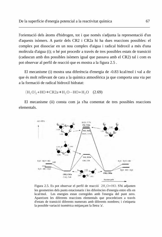
De la superfície d'energia potencial a la reactivitat química 67 __________________________________________________________________
l'orientació dels àtoms d'hidrogen, tot i que només s'adjunta la representació d'un d'aquests isòmers. A partir dels CR2 i CR2a hi ha dues reaccions possibles: el complex pot dissociar en un nou complex d'aigua i radical hidroxil a més d'una molècula d'aigua (i); o bé pot procedir a través de tres possibles estats de transició (cadascun amb dos possibles isòmers igual que passava amb el CR2) tal i com es pot observar al perfil de reacció que es mostra a la figura 2.5 .
El mecanisme (i) mostra una diferència d'energia de -0.83 kcal/mol i val a dir que és molt rellevant de cara a la química atmosfèrica ja que comporta una via per a la formació de radical hidroxil hidratat:
(H2 O)2+HO→CR2a→H2 O−HO+H2O (2.69)
El mecanisme (ii) consta com ja s'ha comentat de tres possibles reaccions elementals.
Figura 2.5. Es pot observar el perfil de reacció 2H2O+HO. S'hi adjunten les geometries dels punts estacionaris i les diferències d'energia entre ells en kcal/mol. Les energies estan corregides amb l'energia del punt zero. Apareixen les diferents reaccions elementals que procedeixen a través d'estats de transició diferents numerats amb diferents nombres; i s'etiqueta la possible variació isomèrica mitjançant la lletra 'a'.
Capítol 2. Estructura electrònica 68 __________________________________________________________________
La primera succeeix a través del TS2a, que mostra una estructura d'anell de tres membres. La reacció consisteix en la ruptura homolítica de l'enllaç O3-H i la formació de l'enllaç H-O1. L'estat de transició queda estabilitzat per dos ponts d'hidrogen; tot i això, la barrera per a CR2a és 13.07 kcal/mol, una mica superior a la de 12.40 kcal/mol trobada en la reacció amb una sola molècula d'aigua. Es pot concloure doncs que el possible efecte catalític degut a les interaccions estabilitzadores dels ponts d'hidrogen a l'estat de transició queden contrarestades per la major estabilitat del complex prereactiu.
Pel que fa als mecanismes que passen per TS3, TS4 i els seus corresponents isòmers són pocs importants degut a la seva energia molt superior. No obstant, com a comentari, val la pena apreciar que TS3 implica una triple transferència de protó i que TS4 implica un tipus de reacció coneguda com a mecanisme de transferència de protó i electró acoblades.
Reacció entre el radical hidroxil i tres molècules d'aigua
Tot examinant aquesta reacció s'han trobat fins a tres isòmers diferents per a cada punt estacionari. La diferència d'energia entre isòmers és petita, com en la reacció amb dues aigües, i tota la discussió s'efectuarà considerant únicament el de més baixa energia.

De la superfície d'energia potencial a la reactivitat química 69 __________________________________________________________________
Després de partir del complex CR3 que incorpora el trímer d'aigua en interacció amb el radical HO es passa per un estat de transició anomenat TS5 que condueix fins a CR4, un anell de quatre membres estabilitzat per ponts d'hidrogen. És destacable el fet de que l'estat de transició mencionat pertany a una zona de la superfície d'energia potencial amb gradients petits. Això fa que els mètodes de localització d'estats de transició siguin difícils de localitzar i aquest en concret no ha pogut ser caracteritzat amb el funcional BH&HLYP sinó amb B3LYP que ha estat també usat per a calcular-ne el punt d'energia zero; això mateix ha passat amb el mínim CR3.
La primera reacció elemental passa per TS6 i implica la ruptura homolítica de l'enllaç O4-H i la formació del H-O1. La barrera és de 13.84 kcal/mol respecte
Figura 2.6. Es pot observar el perfil de reacció 3H2 O+HO. S'hi adjunten les geometries dels punts estacionaris i les diferències d'energia entre ells en kcal/mol. Les energies estan corregides amb l'energia del punt zero. La reacció produeix uns productes idèntics als reactius i degut a això no s'incorpora una il·lustració.
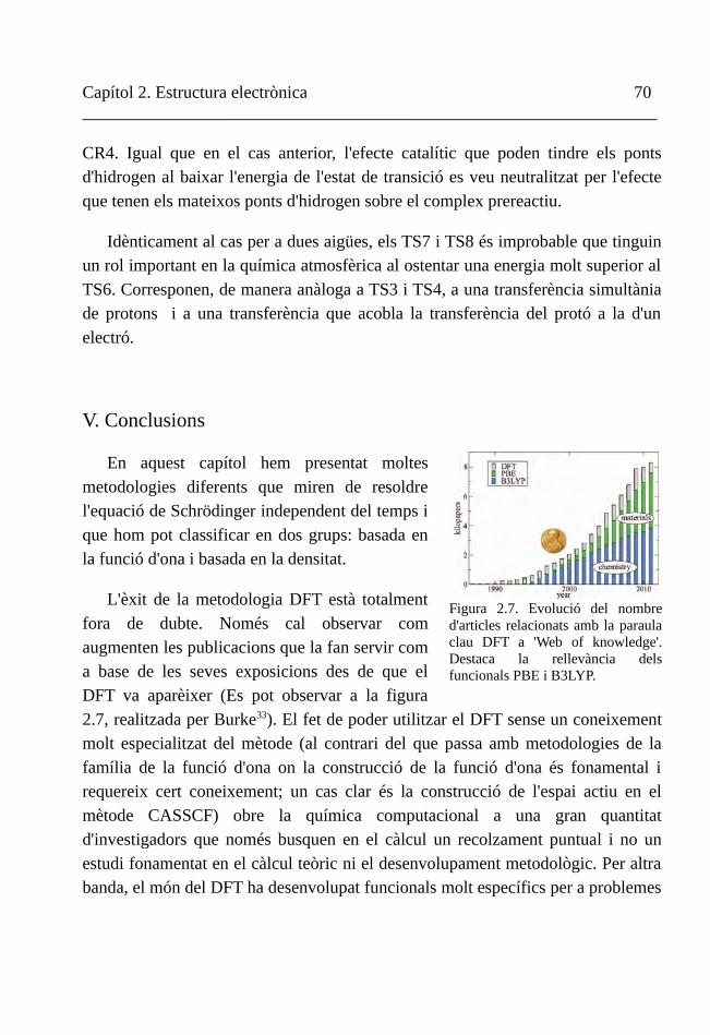
Capítol 2. Estructura electrònica 70 __________________________________________________________________
CR4. Igual que en el cas anterior, l'efecte catalític que poden tindre els ponts d'hidrogen al baixar l'energia de l'estat de transició es veu neutralitzat per l'efecte que tenen els mateixos ponts d'hidrogen sobre el complex prereactiu.
Idènticament al cas per a dues aigües, els TS7 i TS8 és improbable que tinguin un rol important en la química atmosfèrica al ostentar una energia molt superior al TS6. Corresponen, de manera anàloga a TS3 i TS4, a una transferència simultània de protons i a una transferència que acobla la transferència del protó a la d'un electró.
V. Conclusions
En aquest capítol hem presentat moltes metodologies diferents que miren de resoldre l'equació de Schrödinger independent del temps i que hom pot classificar en dos grups: basada en la funció d'ona i basada en la densitat.
L'èxit de la metodologia DFT està totalment fora de dubte. Només cal observar com augmenten les publicacions que la fan servir com a base de les seves exposicions des de que el DFT va aparèixer (Es pot observar a la figura 2.7, realitzada per Burke33). El fet de poder utilitzar el DFT sense un coneixement molt especialitzat del mètode (al contrari del que passa amb metodologies de la família de la funció d'ona on la construcció de la funció d'ona és fonamental i requereix cert coneixement; un cas clar és la construcció de l'espai actiu en el mètode CASSCF) obre la química computacional a una gran quantitat d'investigadors que només busquen en el càlcul un recolzament puntual i no un estudi fonamentat en el càlcul teòric ni el desenvolupament metodològic. Per altra banda, el món del DFT ha desenvolupat funcionals molt específics per a problemes
Figura 2.7. Evolució del nombre d'articles relacionats amb la paraula clau DFT a 'Web of knowledge'. Destaca la rellevància dels funcionals PBE i B3LYP.
De la superfície d'energia potencial a la reactivitat química 71 __________________________________________________________________
molt determinats – satisfent les demandes d'investigadors que es centren en camps molt concrets – però també funcionals tot terreny que donen bons resultats en camps molt diferents i donen seguretat a l'hora d'emprendre estudis en sistemes nous. Per últim, és molt destacable que el DFT és la metodologia dins la química quàntica que millor ataca el problema de la grandària aportant gran quantitat de correlació electrònica: en aquest aspecte no té comparació possible entre els mètodes de funció d'ona que s'han resumit en aquest capítol. Tot i així, la frontera biològica encara li queda lluny.
No es pot ignorar, però, un fet punyent: les implicacions físiques de l'estructura dels mètodes de funció d'ona esmentats estan establertes i són clares. No obstant, un dels punts forts esmentats del DFT (que és innecessari realitzar l'anàleg a construir la funció d'ona del CASSCF o definir la referència per a un MRCI) es tradueix en certa obscuritat com a contrapartida. Tenim en molts casos la quantitat de correlació d'un mètode multiconfiguracional sense necessitat de definir configuracions. Això és sorprenent d'entrada i força positiu; però deixa poques sortides quan el mètode no respon bé, a banda de descartar-lo. En certa manera la conseqüència és que canvia radicalment la manera d'encarar els problemes: és freqüent a la literatura trobar estudis en els que, com a pas preliminar, es posen a prova una sèrie de funcionals i se n'escull el que dóna millors resultats. Això contrasta amb la predicció de l'adequació d'una metodologia i està connectat amb el fet de poder conèixer àmpliament el funcionament intern d'aquesta metodologia i, amb això, fer-se una idea encertada de les seves virtuts i els seus defectes. De l'enfocament apriorístic passem a l'enfocament empíric pel que fa a l'elecció del mètode.
Bibliografia
1. A. Szabo i N. S. Ostlund. Modern Quantum Chemistry: Introduction to Advanced Electronic Structure Theory. Dover Publications (1982)
2. F. Jensen. Introduction to Computational Chemistry. John Wiley & Sons

Capítol 2. Estructura electrònica 72 __________________________________________________________________
(2006)
3. D. Hilbert i R. Courant. Methods of Mathematial Phyiscs, Part 1. Wiley (1953)
4. J. Paldus, Phys. Rev. A, 14, 1620 (1976)
5. B. O. Roos. The Complete Active Space Self-Consistent Field Method and its Applications in Electronic Structure Calculations. A Advances in Chemical Physics. , (2007) 399-445.
6. J. Anglada i J. Bofill, Chemical Physics Letters, 243, 151 (1995)
7. J. M. Bofill i P. Pulay, The Journal of Chemical Physics, 90, 3637 (1989)
8. M. Solà i J. M. Ugalde. Quantum Chemstry Methods: II Density Functional Theory. A Theoretical and Computational Chemistry: Foundations, Methods and Techniques. J. Andrés i J. Bertran (Eds.), (2007) 221-277.
9. R. McWeeny. Methods of Molecular Quantum Mechanics. Elsevier Science (1992)
10. C. Garrod i J. Percus, Journal of Mathematical Physics, 5, 1756 (1964)
11. P. Hohenberg i W. Kohn, Phys. Rev., 136, B864 (1964)
12. O. Gunnarsson i B. I. Lundqvist, Phys. Rev. B, 13, 4274 (1976)
13. W. Kohn i L. Sham, Physical Review, 140, 1133 (1965)
14. I. D. P. R. Moreira, J. M. Bofill, J. M. Anglada, J. G. Solsona, J. Nebot, P. Romea i F. Urpi, Journal of the American Chemical Society, 130, 3242+ (2008)
15. J. Poater, M. Duran, M. Solà i B. Silvi, Chemical Reviews, 105, 3911 (2005)
16. M. J. Frisch, G. W. Trucks, H. B. Schlegel, G. E. Scuseria, M. A. Robb, J. R. Cheeseman, G. Scalmani, V. Barone, B. Mennucci, G. A. Petersson, H. Nakatsuji, M. Caricato, X. Li, H. P. Hratchian, A. F. Izmaylov et al., Gaussian~09 Revision B.1. Gaussian Inc. Wallingford CT 2010.
17. M.W. Schmidt, K.K. Baldridge, J.A. Boatz, S.T. Elbert, M.S. Gordon, J.H. Jensen, S. Koseki, N. Matsunaga, K.A. Nguyen, S. Su, T.L. Windus, M. Dupuis, J.A. Montgomery, Journal of Computational Chemistry, 14, 1347 (1993)
18. M. S. Gordon i M. W. Schmidt. Advances in electronic structure theory: GAMESS a decade later. A Theory and Applications of Computational Chemistry: the first forty years. C.E.Dykstra, G.Frenking, K.S.Kim, G.E.Scuseria (Ed.),

De la superfície d'energia potencial a la reactivitat química 73 __________________________________________________________________
(2005) 1167-1189.
19. Y. Shiota, M. Kondo i K. Yoshizawa, The Journal of Chemical Physics, 115, 9243 (2001)
20. A. Balkova i R. J. Bartlett, The Journal of Chemical Physics, 101, 8972 (1994)
21. H. Worner i F. Merkt, Angewandte Chemie - International Edition, 45, 293 (2006)
22. E. Lee i T. Wright, Physical Chemistry Chemical Physics, 1, 219 (1999)
23. H. Jiao, P. V. R. Schleyer, Y. Mo, M. A. McAllister i T. T. Tidwell, Journal of the American Chemical Society, 119, 7075 (1997)
24. F. Tarantelli, A. Sgamellotti, L. S. Cederbaum i J. Schirmer, The Journal of Chemical Physics, 86, 2201 (1987)
25. M. Caballero, I. D. P. R. Moreira i J. M. Bofill, The Journal of Chemical Physics, 138, 174107 (2013)
26. J. Bofill, I. Moreira i M. Caballero, Molecular Physics, , (2013)
27. P. O. Löwdin, Journal of Mathematical Physics, 3, 969 (1962)
28. P. O. Löwdin. Perturbation Theory and its Application in Quantum Mechanics. Wiley (1966)
29. B. O. Roos, P. R. Taylor i P. E. Siegbahn, Chemical Physics, 48, 157 (1980)
30. J. Gonzalez, M. Caballero, A. Aguilar-Mogas, M. Torrent-Sucarrat, R. Crehuet, A. Solé, X. Giménez, S. Olivella, J. M. Bofill i J. M. Anglada, Theoretical Chemistry Accounts, 128, 579 (2011)
31. M. K. Dubey, R. Mohrschladt, N. M. Donahue i J. G. Anderson, The Journal of Physical Chemistry A, 101, 1494 (1997)
32. E. Vohringer-Martinez, B. Hansmann, H. Hernandez, J. S. Francisco, J. Troe i B. Abel, Science, 315, 497 (2007)
33. K. Burke, The Journal of Chemical Physics, 136, 150901 (2012)

Capítol 3
Teoria del camí de reacció
Fotografia cedida per Brian Chapaitis.

De la superfície d'energia potencial a la reactivitat química 75 __________________________________________________________________
I. Camí de reacció
En el món de la química, i molt especialment en la vessant experimental, hom té una percepció molt concreta sobre quines són les estructures moleculars d'interès: qualsevol que tingui una vida prou llarga com per a ser detectada o, encara millor, per a ser susceptible d'esdevenir un reactiu, producte o intermedi en una síntesi. Anteriorment s'han descrit les característiques de l'energia potencial entesa com a funció de les posicions dels àtoms. No obstant, no s'ha esmentat quines característiques tenen aquests punts en relació amb el seu entorn. Un dels objectius de la química teòrica és relacionar les característiques d'aquest entorn amb les estructures moleculars mencionades. Això es fa a través de les derivades de l'energia potencial respecte les posicions dels àtoms: un punt estacionari en la
superfície d'energia potencial (és a dir, un punt on es satisfà ∇q V=0, on
∇qT=(∂/∂ q1 ,∂/∂ q2 , ... ,∂/∂ qn) i n és la dimensió del vector de coordenades q i 0
és el vector nul) correspon a una geometria totalment estable (reactius, productes o intermedis) si es tracta d'un punt còncau, és a dir, un mínima; si això es compleix, tots els valors propis de la matriu de segones derivades, la hessiana, H , seran
positiusb (∀ i ,HiiD>0, on D indica que es tracta de la matriu diagonal). Si
s'observés alguna convexitat estaríem davant del que en matemàtiques s'anomena punt de sella, l'ordre del qual seria n, on n és el nombre de direccions en les quals la funció potencial és un màxim (és a dir, el valor propi j que hi correspon serà
negatiu, H jjD<0 ). Si el punt de sella és d'ordre 1 seríem davant del que en química
s'anomena estat de transició i correspon a una estructura molecular de molt curta vida. Un punt de sella d'ordre dos és una geometria menys freqüentment tinguda en compte; malgrat això, està constatada la seva rellevància1,2. Si tots els valors propis de la hessiana són negatius tenim un màxim dins la superfície d'energia
a Això es compleix quan l'estructura dels productes correspon a una molècula en equilibri. Si hi ha diverses molècules involucrades, com a reactius i/o productes podem tenir asímptotes en comptes de mínims. Les direccions asimptòtiques corresponen a les coordenades que descriuen la separació de les molècules. És molt comú als processos de dispersió (scattering).
b En el cas de que el sistema de coordenades sigui cartesià hi haurà sis valors propis (cinc si la molècula és lineal) que seran aproximadament zero i s'han d'excloure d'aquest anàlisi. Són els corresponents a rotacions i translacions.
Capítol 3. Teoria del camí de reacció 76 __________________________________________________________________
potencial. Aquest punt estacionari no té un anàleg químic fàcilment assimilable i per tant és de menys interès que els mínims o els punts de sella però al capítol dedicat a trajectòries newtonianes en discutirem la importància. Si en un punt donat es compleix que un valor propi de la hessiana és zero i, a més, el vector propi corresponent és ortogonal al gradient, som davant d'un punt d'inflexió vall-serralada.
Un camí sobre una superfície d'energia potencial es podria definir com una seqüència de diferents geometries moleculars. Matemàticament, això implica una corba. Aquesta corba és estàtica en el sentit que únicament propietats geomètriques de la superfície d'energia potencial són tingudes en compte, sense arribar a incloure cap mena d'energia cinètica. Aquesta corba pot tindre interès per a un químic si ens dóna una noció aproximada de la reactivitat del sistema i aprofundint en aquesta idea arribem al concepte de camí de reacció: si no integrem cap equació sobre la dinàmica del sistema, la millor manera d'aproximar-nos a la reactivitat d'aquest sistema mitjançant una corba és aconseguir que aquesta corba passi pels punts estacionaris més rellevants.
Per exemple, suposem un procés químic que consisteix en una reacció
A ⇄ B ➜ C
Un procés així podria correspondre a la superfície analítica Müller – Brown3, representada a la figura 3.1. Podem veure com el camí proposat connecta efectivament tots els punts estacionaris esmentats. Si prescindim de tot el coneixement apriorístic que teníem sobre la superfície i ens centrem únicament en la informació que ens dóna aquest camí de reacció encara conservem molta informació: diferències d'energia entre conformacions estables; barreres d'energia i forma de les barreres; curvatura del camí. Podem concloure per tant que aquesta corba aporta dades significatives de cara a descriure la reactivitat del sistema proposat. En aquest cas concret s'ha emprat un camí de gradient o camí de la coordenada de reacció intrínseca (IRC); la seva naturalesa serà discutida amb més profunditat en la secció II d'aquest capítol.

De la superfície d'energia potencial a la reactivitat química 77 __________________________________________________________________
Un camí sobre la superfície d'energia potencial pot ser útil però no tot camí sobre la superfície, ni tant sols tot camí útil, és un camí de reacció. Un camí de reacció és una corba contínua que uneix un mínim de la superfície d'energia potencial amb un punt de sella de primer ordre de forma monòtonament creixent i aquest punt de sella amb un segon mínim de forma monòtonament decreixent. El que s'exposa a la figura 3.1 l'és; concretament en tenim dos: un que uneix el mínim A amb el mínim B i un altre que uneix el mínim B amb el mínim C.
Un altre concepte que és freqüent a la bibliografia relacionada amb els camins
Figura 3.1: La reacció que pretenem modelitzar es tracta d'un preequilibri i un producte. Els elements que podem esperar trobar en una superfície d'energia potencial podrien ser per tant els següents: tres mínims, un pel reactiu A (0.5,0), un per l'intermedi B (0,0.5) i un pel producte C (-0.5,1.5); dos estats de transició que connectin A amb B (0.25,0.25) i B amb C (-0.75,0.75) respectivament. Les coordenades són només aproximades.
Capítol 3. Teoria del camí de reacció 78 __________________________________________________________________
de reacció és el de camí d'energia mínima. Un camí de reacció és, a més, un camí d'energia mínima si i només si queda limitat a una vall. Per tal d'identificar una vall es pot projectar la matriu hessiana a l'espai ortogonal al gradient; si la matriu resultant és definida positiva aleshores som a una vall.
II. Coordenada de reacció intrínseca (IRCd)
II.1. Fonamentació matemàtica de l'IRC
Aquest és sense cap mena de dubte el camí més conegut i més present a la literatura. El mètode té els seus orígens als anys setanta i la persona que més va contribuir a desenvolupar-lo en els seus inicis fou Kenichi Fukui4.
La definició matemàtica de la corba IRC és l'equació diferencial de primer
ordre que situa la tangent t [q (s) ] avaluada al punt s de la corba q(s) d'aquesta
corba com a igual al gradient g [q (s )]=∇ q V normalitzat al mateix punt:
t [q (s) ]=d q(s)
d s=
g [q(s)]∣g [q(s)]∣
(3.1)
S'ha relacionat aquesta corba amb principis variacionals diverses vegades, una de les més recents observant que satisfà una equació tipus Hamilton – Jacobi5.
Per tal d'arribar a aquesta equació per mitjans de la teoria de càlcul de variacions es parteix de la consideració de que la corba és un camí propagant-se en un medi, la superfície, emprant el camí de mínima energia. De totes les possibles
corbes q(s) – que comencen al punt q (0) i acaben al punt q (s) – i que
minimitzen la integral
d De l'anglès Intrinsic Reaction Coordinate.

De la superfície d'energia potencial a la reactivitat química 79 __________________________________________________________________
ΔV=∫0
sdsμ(s)
(3.2)
on el paràmetre s és la longitud d'arc i μ(s) fa el paper de la inversa d'una
velocitat en aquest modele. Integrant la inversa de μ(s) obtenim la distància
geodèsica sobre la superfície d'energia potencial entre els dos punts que corresponen als límits de la integral. Per tal de connectar aquesta visió amb el camí
IRC es pren μ(s)=∣g [q(s)]∣−1
i es realitza un canvi de variable: la corba passarà a
estar definida amb el paràmetre t que es defineix de la manera següent:
ds=√(d qdt )
T
( d qdt )dt (3.3)
Substituint a l'equació (3.2) obtenim una reformulació del problema, ja que la podem expressar com a:
ΔV=∫0
t
√gT g( d qdt )
T
( d qdt )dt=∫
0
t
F (q , dq /dt)dt (3.4)
En aquesta equació hem emprat g=g(q(s)) . La integral és homogènia d'ordre
1 respecte la tangent d q/dt i no depèn explícitament del paràmetre t que parametritza la corba. Realitzant la variació de primer ordre d'aquesta integral i igualant-la a 0 podem trobar la corba que minimitza el funcional integral; finalment, es resol l'equació d'Euler - Lagrange i s'arriba a l'equació (3.1), demostrant inequívocament el caràcter variacional de la corba IRC.
Aquest és el camí de reacció que s'ha emprat a la figura 3.1. Es pot observar visualment com la corba és en tot moment ortogonal als nivells equipotencials degut a que la seva tangent té en tot moment la mateixa direcció que el gradient. La mena d'informació que aquest camí aporta sobre la reacció química ha estat comentada al final de l'apartat anterior.
e ν(s) es pren com a sempre positiva.

Capítol 3. Teoria del camí de reacció 80 __________________________________________________________________
Al capítol 4 es discutirà l'hamiltonià del camí de reacció que està basat en aquesta corba concreta.
Per completar la discussió, es pot obtenir l'equació de Hamilton-Jacobi a partir de les igualtats següents:
p=∇ dqdt
F(q ,d q /dt)=(gT g )1/2d q/dt
(d q /dtT dq /dt)1 /2=∇q S (q)
on la darrera igualtat és la derivada de l'acció respecte el vector de posicions.
Si definim
G(q)=g (q)T g (q ) (3.5)
podem trobar una equació tipus Hamilton-Jacobi com la següent:
d q /dt∣d q /dt∣
=∇q S (q)
G(q)1 /2
Addicionalment, és possible escriure la següent igualtat que es coneix com a equació eikonal o equació de Hamilton – Jacobi estàtica d'una corba de camí de gradient en el domini d'una superfície d'energia potencial.
(∇q S (q))T (∇q S (q))=G(q)
Les equacions eikonals es relacionen sovint amb problemes de propagació d'ones. Podem per tant connectar els camins IRC amb aquest fenomen físic.
II.2. El camí de gradient com a mitjà per associar una ona a una superfície d'energia potencial6
Podem fer una lectura de l'equació funcional integral 3.4 segons la qual, quan

De la superfície d'energia potencial a la reactivitat química 81 __________________________________________________________________
en practiquem la primera variació, cerquem la mínima integral possible en el camí d'aquesta funció G(q). L'equació s'expressaria doncs com a:
ΔV=∫0
t
√G(q )( dqdt )
T
( d qdt )dt (3.6)
Durant l'evolució del paràmetre t es produeix també l'evolució del vector
posició q=q IRC(t ) que coincideix amb les posicions permeses en el camí IRC;
també es produeix el canvi del potencial V (q)=ν i podem realitzar la
interpretació de que la corba va creuant línies d'equipotencial de manera ortogonal on aquest potencial constant a tota la línia és igual a ν . És important adonar-se del fet de que les corbes només tallen les línies d'equipotencial en un punt i de que evolucionen monòtonament entre punt estacionari i punt estacionari: això ens permet afirmar que hi ha una relació u a u entre la corba i el valor d'energia del membre de la família de línies de contorn. Degut a aquest fet, podem realitzar un
nou canvi de parametrització a la corba i passar de q (t) a q (ν) 7. Està
demostrat8 que la solució d'una l'equació (3.5) és una família de línies d'equipotencial. El fet de que aquesta solució respon al principi de Fermat – Huygens per a la construcció de fronts d'ones també és conegut5,9,10. L'equació resultant hauria de tenir una forma com la següent:
∇q2ψ(q , ν)−G(q ) ∂
2
∂2νψ(q , ν)=0 (3.7)
on ∇q2=∇q
T∇q=∂
2/∂ q1
2+...+∂2
/∂ qn2 . Aquesta equació intenta satisfer el principi
de Fermat – Huygens des del punt de vista més general possible; i per això s'entén que les senyals nítides es propaguen com a senyals nítides. Aquí una 'senyal' és un nivell d'equipotencial d'una superfície d'energia potencial.
Per tal de resoldre aquesta mena d'equacions diferencials8 amb derivades parcials s'utilitza el mètode de característiques. Generalment s'utilitza per a equacions diferencials parcials de primer ordre, però en el nostre cas també és aplicable per a aquesta equació hiperbòlica de segon ordre. La idea és la de trobar
Capítol 3. Teoria del camí de reacció 82 __________________________________________________________________
les anomenades corbes característiques, a través de les quals les equacions diferencials parcials esdevenen una família d'equacions diferencials ordinàries fàcilment integrables. Es compara l'equació de partida amb el vector director d'un pla i en conseqüència s'obté un seguit d'equacions que són comparades a corbes contingudes al pla que el propi vector director defineix. En el nostre cas, de totes les solucions possibles, estem interessats en el pla característic que satisfà l'equació (3.7) (Apèndix A). Aquest pla ve donat per:
∑i=1
N
ϕqi
2−G(q)ϕν2=0 (3.8)
A l'equació (3.8), ϕqi és la derivada respecte q i de la funció característica ϕ i
ϕν és la derivada respecte ν de la mateixa funció característica. Es pot observar
com les equacions característiques defineixen conoides si no són a un punt estacionari. Qualsevol punt de la superfície d'energia potencial es pot considerar adscrit en un pla definit per la següent equació:
((q−q0)T , (ν−ν0))( ∇qϕ ∣q=q0
∂ϕ /∂ ν∣q=q0
)=0 (3.9)
Anomenarem vector r al resultat de la normalització del vector
(∇qTϕ , ∂ϕ/∂ ν) . Ja que l'equació característica (3.8) és homogènia respecte
aquest nou vector, podem introduir-hi aquest vector obtenint:
rqT rq−G(q)r ν
2=[(rqT rq)
1 /2+G(q)1 /2 rν ]−[(rqT rq)
1/2−G(q )1/2r ν ] (3.10)
on s'ha descompost el vector r en els components que contenen derivades respecte
q , rq , i l ' element queconté una derivada respecte ν , rν . A la part dreta de la
igualtat s'hi poden identificar dos termes diferenciats: el primer correspon a un conoide en un sentit 'directe' i el segon a un conoide en el sentit invers. Utilitzant el fet de que r és un vector normalitzat, la part esquerra de la igualtat es pot transformar de la següent manera

De la superfície d'energia potencial a la reactivitat química 83 __________________________________________________________________
rqT rq−G(q)rν
2=1−(1+G(q))rν
2=0 (3.11)
I, d'aquí,
rν=1
(1+G(q))1/2
(rqT rq)
1 /2=
G1/2(q )
(1+G(q))1 /2
(3.12)
que són el cosinus del vector normal al pla característic i l'eix ν i el radi del 'cercle' del conoide en la seva intersecció amb la hipersuperfície característica amb energia ν . Amb aquesta informació podem construir esquemàticament els conoides que corresponen a les característiques de l'equació hiperbòlica com es reflexa a la figura 3.2.
Figura3. 2: Representació esquemàtica del conoide en sentit directe descrit a l'equació (3.10), en tres dimensions. S'ha pres G(q)=1.
Capítol 3. Teoria del camí de reacció 84 __________________________________________________________________
Escollint una funció
Per tal de resoldre l'equació 3.8 es proposa com a funció de prova
ϕ(q , ν)=exp (i [ν−V(q)])−1 (3.13)
que la satisfà tal i com es pot comprovar de manera trivial, ja que es recupera l'equació eikonal de partida, 3.5. Addicionalment, per a una ϕ constant i igual a 0
el potencial ha de ser ν=V(q) .
No obstant, aquesta funció de prova no compleix l'equació 3.7. Degut a la regla de la cadena, apareix el terme −tr H∂/∂ ν , on tr H és la traça de la matriu hessiana. Nogensmenys, podem modificar l'equació introduint aquest terme en sentit contrari on el terme en qüestió jugaria el paper d'una fricció.
(∇q2−G(q) ∂
2
∂ν2 +tr H ∂∂ν )ψ(q , ν)=0 (3.14)
Podem prendre una forma més general de la funció d'ona que mantingui l'estructura anterior amb primera i segona derivades contínues i funció d'una variable real F(x).
Ψ(q , ν)=F (ν−V(q)) (3.15)
És interessant destacar que per a tr H>0 el terme, com a fregament, seria afísic.
Un problema característic de valors inicials amb solució única
No hauria de sorgir cap punt estacionari entre un punt q (t0) a una
hipersuperfície amb ν0 i el corresponent q (t f ) a una hipersuperfície amb la seva
corresponent νf . Avaluem ara si per a una equació d'ones de segon ordre com la
equació 3.7 és possible tenir un problema característic de valors inicials amb

De la superfície d'energia potencial a la reactivitat química 85 __________________________________________________________________
solució única. Prenem una solució tal com
∣Ψ(q , ν)∣ν=V (q)=F(ν −V(q ))=F (0)=0 (3.16)
a tota la superfície. A més també assumim sense pèrdua de generalitat que
F(0)=0. Vegem les implicacions que això té sobre l'equació 3.8. Si la
multipliquem per −2ψν obtenim
2ψν(G(q)ψν ν−∑i=1
N
ψqi qi)=0 (3.17)
on els índex indiquen la corresponent derivació. Això és igual a:
(G(q) ψν2)ν−2∑
i=1
N
(ψqiψν)qi
+∑i=1
N
(ψqi
2)ν=0 (3.18)
L'equació 3.18 és una divergència. Per integració en tot el volum del doble conoide i l'aplicació del teorema integral de Gauss permet expressar la següent integral de superfície:
∫∫DC[(G(q)ψν2)rν−2∑
i=1
N
(ψqiψν)rqi
+∑i=1
N
(ψq i
2)r ν]dS=0 (3.19)
que al seu torn es pot expressar recordant les equacions 3.12 com a
∫∫DC[ 1r ν∑i=1
N
(ψqir ν−ψν rqi
)2]dS=0 (3.20)
i aquesta integral és la prova de la unicitat de la solució del problema característic de valors inicials: ja que la integral es nul·la, l'integrant també ho és donat que es tracta de la integral d'un quadrat.
Capítol 3. Teoria del camí de reacció 86 __________________________________________________________________
Tornem al camí de gradient
La solució que oferim a l'equació 3.14 és Ψ(q , ν) sota les condicions
F(ν −V(q ))=F (0)=0 ; i això implica una hipersuperfície S. La funció Ψ(q , ν)
ha de tenir segona derivada contínua. Les dades de la superfície S consisteixen en
Ψ(q , ν) i el conjunt de les seves primeres derivades respecte de q i ν . Si es dóna
la circumstància de que podem construir un sistema lineal d'equacions que ens
doni la solució Ψ(q , ν) com a solució a 3.14 amb primera i segona derivada
contínua en S direm que la hipersuperfície és no característica. En canvi, si no es satisfà això direm que és característica. Per exemple, un punt en el que
ν −V (q)=0, les derivades de la funció d'ona tal i com es planteja no seran
contínues.
Plantegem que G(q) pot ser qualsevol funció. Podem emprar l'equació 3.5 de la següent manera:
Q(∇q V , q)=∇ qT V (q)∇ q V (q)−G(q ) (3.16)
Es complirà que Q(∇q V , q)=0 sempre que la nostra ona es propagui en un
camí de gradient i aquesta és la nostra condició característica que ens permet establir un conjunt d'equacions. Però recordem també que aquesta és l'equació de Hamilton – Jacobi per a un camí de gradient, així que prendrem l'equació 3.16 com a hamiltonià d'un cert problema. Podem aleshores desenvolupar les equacions de
Hamilton – Jacobi. La nostra funció depèn de les variables ∇q V i q . Per tant, la
primera equació, que és la pròpia de l'IRC sense normalitzar, 3.1, serà la següent:
dqdt=
12∇∇ qV Q(∇q V , q)=∇ q V (q )=g (t) (3.17)
La segona equació serà:
d gdt=−
12∇ q Q(∇ q V , q) (3.18)

De la superfície d'energia potencial a la reactivitat química 87 __________________________________________________________________
però degut a la igualtat anterior (3.17), és possible escriure:
dgdt=∇q gT d q
dt=∇ q∇q
T V (q)g( t)=H(t)g (t) (3.19)
i també és interessant denotar que és possible expressar:
d gdt=
ddt (
d qdt )=
d2 qdt 2 (3.20)
això és molt rellevant perquè implica que l'equació és de fet la segona derivació de l'equació 3.17 i per tant només existeixen N equacions que defineixen el comportament del nostre sistema i que ens donen totes les corbes característiques
per a la solució ψ(q ,ν) . A més, aquestes corbes integrals són els rajos
característicsf de l'equació diferencial parcial de segon ordre 3.7 o 3.14 perquè generen tots els membres de la família d'hipersuperfícies d'energia potencial
ν=V (q) . Les hipersuperfícies característiques de l'equació 3.16 fan el paper de
fronts d'ona. El que obtenim finalment és una solució Ψ(q , ν) a la que li
correspon una superfície; i a cada punt d'aquesta superfície li correspon un punt
d'una superfície anterior amb V (q)=ν0 . Per a l'equació 3.14, veiem que tenim la
propagació d'un front d'ones V (q)=ν0 en direcció a les hipersuperfícies
d'equipotencial paral·leles V (q)=ν per a qualsevol ν .
Cada hipersuperfície d'equipotencial paral·lela depèn de l'anterior igual que la següent dependrà d'aquesta. Aquí trobem un fort paral·lelisme amb el principi de propagació de fronts d'ones de Huygens11. Segons el seu tractat, el front d'ones d'una ona lumínica es propaga com a l'envolupant de les ones que emanen de cada punt del front d'ones de l'instant anterior, tenint en compte que aquestes ones es propaguen a la mateixa velocitat que el conjunt de l'ona resultant.
En el nostre cas, a través de les diverses corbes integrals del camí de gradient, al crear una hipersuperfície d'energia ν constant donada, estem creant també una
f Les corbes integrals que generen totes les altres per a una equació diferencial donada

Capítol 3. Teoria del camí de reacció 88 __________________________________________________________________
envolupant que resulta en un front d'ones. I podem considerar aquestes hipersuperfícies com a les ones que es generen a cada punt del front d'ones anterior
on les hipersuperfícies es generaven amb una energia constant ν0 donada.
III. Gradients extremals
III.1. Fonamentació matemàtica dels gradients extremals
Els gradients extremals són corbes en les quals es compleix que en tots els punts de la corba el gradient és un vector propi de la matriu hessiana12. És a dir, en tot punt q de la corba es satisfà la següent equació de valors i vectors propis:
Hg=λ(q)g (3.21)
Hom també sol destacar com a característica definitòria el fet de que en creuar una línia d'equipotencial, el GE ho farà sempre per un punt en el que l'arrel
quadrada de la norma del gradient, gT g , és un extrem respecte el seu entorn en aquella línia d'equipotencial.13
Recentment, s'ha pogut plantejar l'equació de la corba de GE com una solució a un problema variacional14.
Figura3. 3: les ones parteixen d'una corba de nivell anterior i construeixen un nou front d'ones que és la nova corba de nivell.

De la superfície d'energia potencial a la reactivitat química 89 __________________________________________________________________
L'objectiu és aconseguir que la següent integral sigui estacionària:
I (q)=∫t o
tf
F (t ,q)d t=∫to
tf
gT gd t (3.22)
És a dir, partim no de la primera característica dels gradients extremals esmentada sinó a partir de la segona. És convenient destacar que la corba definida per les coordenades q està en aquesta ocasió parametritzada mitjançant el paràmetre t. De manera que tant q com el gradient g depenen implícitament de t: g=g(q(t )) .
A més de les condicions de contorn que suposen els límits de la integral definida, s'introdueix una nova condició a través d'un multiplicador de Lagrange. La condició és:
G(q ,t)=V (q)−ν(t)=0 (3.23)
Aquí, ν(t ) és la funció que té com a domini el paràmetre t i com a codomini
el valor del potencial que li correspon.
La integral funcional de la qual volem trobar el punt estacionari serà doncs la següent:
I (q)=∫t 0
tf
L(q ,t )dt=∫t0
tf
[F (q , t)−λ(q (t))G(q , t)]d t
=∫t0
tf
[gT g−λ(q (t))(V (q )−ν(t ))]d t (3.24)
On s'ha denominat λ (q) al multiplicador de Lagrange amb dependència de t a
través de q. Segons el càlcul de variacions, a cada punt es satisfarà la següent igualtat que caracteritzarà la corba extremal:
Hg−[V (q )−ν]∇q λ (q)−λ(q )g=0 (3.25)
Capítol 3. Teoria del camí de reacció 90 __________________________________________________________________
i aquesta serà l'equació d'Euler – Lagrange del sistema. És destacable el fet de que hem abandonat tota dependència respecte al paràmetre t. Degut a la restricció 3.23 podem reduir aquesta equació a:
Hg−λ(q)g=0 (3.26)
que és una equació de vectors i valors propis on en tot moment el valor propi de la hessiana serà el gradient. Hem definit correctament, per tant, la corba de gradients extremals.
Des del punt de vista teòric aquesta equació és suficient però la seva vessant pràctica és molt limitada. El que esperem d'una equació que caracteritzi una corba és que contingui la tangent dq /d t en algun dels seus termes per tal de poder integrar la corba, és a dir: per a un increment infinitesimal dt poder calcular a
quina q (t f ) podem arribar des d'una q (t0) . Per tal de fer-ho, s'ha emprat teoria
de pertorbacionsg.
Abans de poder-la aplicar, però, cal realitzar unes modificacions a les equacions obtingudes ja que el multiplicador de Lagrange no és convenient de cara al tractament de les equacions. Per fer-ho, partint de l'equació 3.26
multiplicarem gT/gT g per la dreta i la transposada de 3.26 per l'esquerra per
g /gT g . Obtindrem dues equacions que restarem recordant que HT=H :
HggT
gT g−λ(q )
gT
gT g=0
g
gT ggT H−λ(q)
g
gT g=0
} Hg gT
gT g−
g gT
gT gH=0 (3.27)
Si anomenem el projector a l'espai del gradient ggT
gT g=P podem escriure
H P−P H=O on O és la matriu tots els elements de la qual són igual a zero.
g La mateixa que proposà McWeeny per tal d'aplicar-la a problemes d'estructura electrònica15.
De la superfície d'energia potencial a la reactivitat química 91 __________________________________________________________________
Addicionalment, necessitem que el vector propi estigui normalitzat. El
prendrem, per tant, dividit per la seva norma: gT /√gT g g/√gT g=1 . Comprovem també la idempotència del projector:
PP=g gT
gT gg gT
gT g=
g gT
gT g=P (3.28)
Amb aquestes propietats en ment, desenvoluparem utilitzant teoria de pertorbacions tant la hessiana H com el projector P al voltant del punt
q=q0=q (t 0) fins a segon ordre:
P=P0+(t−t 0)dPd t ∣q=q0
+(t−t 0)
2
2d2 Pd t2 ∣
q=q0
=P0+( t−t0)P0(1)+( t− t0)
2
2P0(2)(3.29)
H=H0+(t−t 0)d Hd t ∣q=q0
+(t−t 0)
2
2d2 Hd t 2 ∣
q=q0
=H0+(t−t0)H0(1)+( t−t0)
2
2H0(2)(3.30)
Aquí H0 i P0 representen la hessiana i projector al punt q0 sense cap
pertorbació, respectivament. Prenent les dues equacions anteriors fins a primer ordre i substituint-les a HP−PH=O es dedueix la següent igualtat:
(H 0 P0(1)+H0
(1)P0)+(P0 H0(1 )+P0
(1 )H0)=0 (3.31)
La idempotència (3.28) sota l'efecte de la pertorbació a primer ordre ens condueix a la següent expressió:
P0 P(1)+P(1)P0=P(1) (3.32)
Això implica que l'estructura de P(1) sigui la següent:
P(1)=(1−P0)M0 P0+P0 M0T(1−P0) (3.33)
per tal de preservar la idempotència. I que en el nostre cas concret, la matriu

Capítol 3. Teoria del camí de reacció 92 __________________________________________________________________
M0 sigui la següent:
M0=H0∣d qdt ∣q=q0
g0T
g0T g0
=H0 t0
g0T
g0T g0
(3.34)
on t 0 és el vector tangent al voltant del punt q0 . Aquesta estructura ve donada
per la derivació del projector respecte t que en aplicació de la regla de la cadena
implica la seva derivada parcial respecte del vector q: d /dt=tT∇ q . Si emprem
les equacions 3.31 i 3.33 i multipliquem per esquerra i dreta per (1−P0) i P0 ,
respectivament, obtenim la següent expressió:
(1−P0){H0(1−P0)M0+H(1)P+MH0 P }=0 (3.35)
Aquesta expressió ja conté tota la informació sobre la corba de gradient extremal i la seva tangent. Per tal de visualitzar-la de manera explícita, simplement
hem de tenir en compte que (1−P0)H0 P0=0 degut a la naturalesa dels gradients
extremals (específicament, tenint en compte l'equació 3.26) i multiplicar-la per la
dreta per g0 . Obtindrem
(1−P0){H02 t 0+H(1)g0−H0 t0
g0T H0 g0
gT g }=0 (3.36)
Si mirem d'obtenir l'estructura del producte H(1)g trobarem que a l'equació de la corba dels gradients extremals s'hi veu implicat el tensor de terceres derivades
del potencial respecte de la posició, F0 . El producte tensorial amb el gradient fa
que finalment el rang terme sigui 2, el propi d'una matriu:
⟨ d H0
d t ⟩g0=⟨∇q H0
dq0
d t ⟩ g0=⟨F0 t0 ⟩g0= ⟨F0 g0 ⟩ t0 (3.37)
Si desenvolupem aquest producte dins l'equació 3.36, podem separar la tangent
t 0 obtenint finalment una expressió integrable.

De la superfície d'energia potencial a la reactivitat química 93 __________________________________________________________________
(1−P0){H02+ ⟨F0g0 ⟩−H0
g0T H0 g0
g0T g0
}t0=0 (3.38)
Aquesta equació fou obtinguda per primer cop per Sun i Ruedenberg.16
De cara a fer-la més tractable, encara s'hi poden introduir modificacions utilitzant les propietats que venen donades per l'equació 3.26. El subespai definit
per 1−P0=V0 V 0T ve donat per una matriu de dimensions N x N-1 que conté els
vectors propis de la diagonalització de H0 excepte el vector propi colineal al
gradient; òbviament, serà un conjunt ortogonal al gradient, formant un conjunt ortonormal amb ell. També considerarem la divisió del vector tangent en dos components, un projectat sobre cada subespai:
t 0={P0+(1−P0)}t0=g0 g0
T
g0T g0
t0+V0 V 0T t0=
g0
g0T g0
eg0+V0 eN−1
0(3.39)
El component eg0 és un escalar i el component eN−1
0 un vector de N-1
dimensional.
Amb les equacions 3.38 i 3.39 es pot arribar a una nova equació que defineix la corba extremal:
−V0T ⟨F0 g0 ⟩
g0
√g0T g0
eg0=V0
T {H02+ ⟨F0 g0 ⟩−H0
g0T H0 g0
g0T g0
}V0 eN−10
(3.40)
Tenint en compte que som sobre la corba extremal, els vectors en V 0 són tots
els que diagonalitzen la matriu H0 excepte pel que fa al vector g. Per tant,
V0T H V0=HN−1
D . Degut a l'ortonormalitat de la base de vectors propis també es
satisfarà que V 0T H0 g0/∣g0∣=V0
T g0/∣g0∣=0N−1 i, lògicament, V0T V0=IN−1 ; on I és
la matriu identitat amb dimensió N-1 x N-1 i 0 és el vector zero amb dimensionalitat N-1. Per tal de poder integrar la corba, necessitem conèixer tots

Capítol 3. Teoria del camí de reacció 94 __________________________________________________________________
dos components de la tangent. Si en coneixem un, l'altre es pot determinar per
condició d'ortogonalitat. Per tant, per resoldre el valor de la tangent, aïllarem eN−10
. Això implica que el determinant de tota la matriu que multiplica aquest vector sigui no nul per tal de poder-ne fer la inversa. Si no ho fos, es pot demostrar que estem en un punt de retorn o en un punt de bifurcació14. Un punt de retorn és aquell punt en el que la corba no creua la línia de contorn de potencial sinó que només la toca tangencialment. Un punt de bifurcació és un punt on es creuen dues corbes de gradients extremals. A la figura 3.4 es poden observar ambdós.
Fins ara s'ha demostrat el caràcter extremal d'aquestes corbes. Addicionalment, és possible establir les condicions en les quals aquestes corbes són mínims; serà
doncs necessari que es compleixi la inequació δ2 I≥0 i això es fa dins el marc de la teoria de càlcul de variacions8.
Figura 3. 4: Es pot observar com els gradients extremals connecten dos punts de sella senyalitzats com a 'SP' i passen per un punt d'inflexió vall – serralada marcat amb 'VRI'. Podem observar que els punts de sella actuen com a punts de bifurcació i dos punts de retorn: un entre cada punt de sella i el punt d'inflexió vall-serralada. Aquesta superfície es presenta més endavant en el seu conjunt.
De la superfície d'energia potencial a la reactivitat química 95 __________________________________________________________________
III.2. Com ens ajuden els gradients extremals a entendre una reacció química
A la secció I s'ha argumentat per què un camí IRC és un bon referent per conèixer de manera aproximada la reactivitat d'un sistema: el fet de que el camí de reacció passi per tots els punts que representen geometries rellevants a la reacció permet que la reacció en sí quedi ben descrita. Ara bé, la simplicitat del model obre la porta a que sigui relativament fàcil trobar casos en els que la representació d'aquest tipus de camí de reacció no sigui aconsellable.
L'exemple que es proposa és l'esquema d'una reacció composta de tres reaccions paral·leles o competitives de l'estil:
A ⇄ B
A⇄ C
B ⇄ C
Una sistema com aquest ve representat per una superfície d'energia potencial com la representada a la figura 3.517.
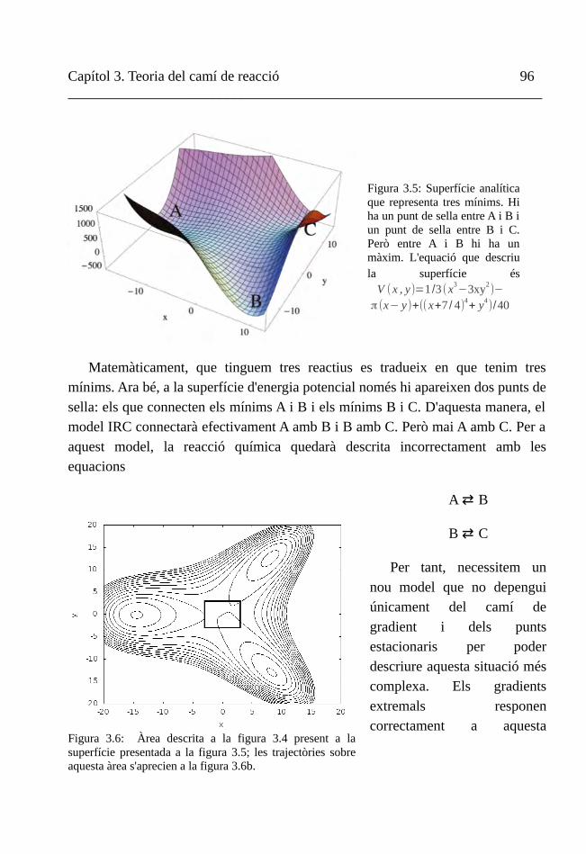
Capítol 3. Teoria del camí de reacció 96 __________________________________________________________________
Matemàticament, que tinguem tres reactius es tradueix en que tenim tres mínims. Ara bé, a la superfície d'energia potencial només hi apareixen dos punts de sella: els que connecten els mínims A i B i els mínims B i C. D'aquesta manera, el model IRC connectarà efectivament A amb B i B amb C. Però mai A amb C. Per a aquest model, la reacció química quedarà descrita incorrectament amb les equacions
A ⇄ B
B ⇄ C
Per tant, necessitem un nou model que no depengui únicament del camí de gradient i dels punts estacionaris per poder descriure aquesta situació més complexa. Els gradients extremals responen correctament a aquesta
Figura 3.5: Superfície analítica que representa tres mínims. Hi ha un punt de sella entre A i B i un punt de sella entre B i C. Però entre A i B hi ha un màxim. L'equació que descriu la superfície és
V (x , y)=1 /3 (x3−3xy2
)−
π(x− y)+((x+7 / 4)4+ y4)/40
Figura 3.6: Àrea descrita a la figura 3.4 present a la superfície presentada a la figura 3.5; les trajectòries sobre aquesta àrea s'aprecien a la figura 3.6b.

De la superfície d'energia potencial a la reactivitat química 97 __________________________________________________________________
necessitat com es pot observar a la figura 3.4 que correspon a l'àrea de la superfície marcada amb un marc a la figura 3.6. Certament, les corbes que emergeixen de cada mínim tenen un punt de trobada en el punt marcat com a VRI, un punt d'inflexió.
Anàlisi de la validesa del camí de reacció mitjançant dinàmica
Aquesta apreciació des del nostre model estàtic es pot recolzar amb càlculs dinàmics.
Si analitzem trajectòries clàssiques partint al mínim A i seguint les equacions de Newton (figura 3.7) es pot observar com es prediu reactivitat tan en el sentit de B com en el de C. Si ens centrem en el marc proposat a la figura 3.6, destaquem part d'una sèrie de trajectòries tal i com s'aprecia a la figura 3.6b.
Figura 3.7: Trajectòries clàssiques sobre la superfície descrita al text. Les trajectòries comencen al mínim A i tenen un moment inicial diferent de manera que s'escombra tot un rang de possibles direccions.
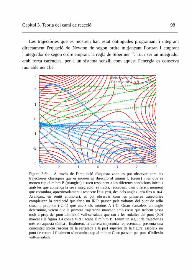
Capítol 3. Teoria del camí de reacció 98 __________________________________________________________________
Les trajectòries que es mostren han estat obtingudes programant i integrant directament l'equació de Newton de segon ordre mitjançant Fortran i emprant l'integrador de segon ordre emprant la regla de Stoermer 18. Tot i ser un integrador amb força carències, per a un sistema senzill com aquest l''energia es conserva raonablement bé.
Figura 3.6b: A través de l'ampliació d'aquesta zona es pot observar com les trajectòries clàssiques que es mouen en direcció al mínim C (creus) i les que es mouen cap al mínm B (triangles) actuen responent a les diferents condicions inicials amb les que comença la seva integració: es tracta, recordem, d'un diferent moment que escombra, aproximadament i respecte l'eix y=0, des dels angles -π/4 fins a π/4. Avançant, en sentit antihorari, es pot observar com les primeres trajectòries compleixen la predicció que faria un IRC: passen pels voltants del punt de sella situat a prop de (-2,-1) que uneix els mínims A i C. Quan s'assoleix un angle determinat, veiem que la primera trajectòria marcada amb creus que trobem passa molt a prop del punt d'inflexió vall-serralada que rau a les rodalies del punt (0,0) marcat a la figura 3.4 com a VRI i acaba al mínim B. Tenim un seguit de trajectòries més en aquesta tònica i finalment, la darrera trajectòria representada, presenta una curiositat: inicia l'ascens de la serralada a la part superior de la figura, assoleix un punt de retorn i finalment s'encamina cap al mínim C tot passant pel punt d'inflexió vall-serralada.

De la superfície d'energia potencial a la reactivitat química 99 __________________________________________________________________
Figura 3.8: Propagació quàntica sobre la superfície descrita al text. Es mostra la seqüència de
tota la dinàmica del paquet d'ones amb moment inicial amb direcció (1,0). S'hi aprecia com el paquet d'ones es divideix i acaba ocupant parcialment els mínims A, B i C.
Si propaguem un paquet d'ones utilitzant el codi MCTDH19 de Meyer i col·laboradors, observem de nou que es prediu la generació tant del producte B com del producte C tal i com es pot observar a la figura 3.8. No obstant, també
Capítol 3. Teoria del camí de reacció 100 __________________________________________________________________
apreciem qualitativament la major formació de C.
El camí basat en gradients extremals dóna, per tant, una imatge molt més encertada de la reactivitat del sistema que la que pot arribar a donar un de basat en corbes tipus IRC.
IV. Trajectòries de l'ascens gradual
IV.1. Fonamentació matemàtica i precedent
Recentment, E i Zhou20 han proposat un nou tipus de corba anomenada ascens gradual. Aquest mètode es pot entendre com la reformulació d'un altre de més anterior proposat per Smith21,22. El mètode de Smith es basa en associar una funció imatge a la superfície d'energia potencial; en aquesta imatge hi ha un mínim on a la superfície sota estudi hi ha un estat de transició, de manera que els algoritmes que s'apliquen per tal de trobar mínims són útils per tal de localitzar-lo. El mètode té una aplicabilitat limitada ja que, tal i com van demostrar Sun i Ruedenberg, les funcions imatge generalment no existeixen en superfícies d'energia potencials excepte a les rodalies de punts crítics; per tant, una cerca de mínims per tal de localitzar estats de transició pot resultar inadequada.23
En aquesta mateixa referència, es defineix una família de funcions imatge del
potencial V (q) , que anomenem W (q ) . A més, es relaciona el gradient g(q) de la
superfície d'energia potencial amb la seva imatge f(q) mitjançant la següent equació diferencial:
f (q)=Uv g(q)=[I−2v (q)vT
(q)
vT(q)v (q) ] g(q ) (3.41)
on U v és la coneguda com a matriu ortogonal de Householder24 construïda a
partir d'un vector arbitrari v(q) i I és la matriu unitat. Tal i com està definida, la

De la superfície d'energia potencial a la reactivitat química 101 __________________________________________________________________
matriu de Householder es comporta com un pla de reflexió amb vector director
v(q): es comprova fàcilment que Uv v (q )=−v (q ) i també que, per a un vector u
donat tal que vT(q)u=0 , U v u=u . Té la propietat de que Uv=Uv
T i la seva
expressió és conseqüència de que, trivialment, Uv=(I−Pv)−Pv=I−2Pv , essent
Pv=v (q) vT
(q)
vT(q )v (q)
(3.42)
Diferenciant respecte q l'equació (3.41) corresponent al gradient a la superfície imatge obtenim una expressió que conté la imatge de la Hessiana,
F(q )=Uv H(q ) juntament amb un altre terme:
∇q fT(q)=∇ q(g
T(q)Uv)=FT
(q)+gT(q)∇ qUv=FT
(q )−2gT(q )∇q Pv (3.43)
En aquest segon terme, la derivada del projector és generalment no zero i no simètrica. Degut a la influència d'aquest terme es complirà que:
(∇q fT(q))ij−(∇q f T
(q )) ji≠0 amb i≠ j (3.44)
i aquesta desigualtat implica que el camp del gradient definit a l'equació 3.41 no és integrable:
W (q1)−W (q0)≠∫t0
t 1
f T (q )(d q/dt )dt (3.45)
Aquí d q/dt és la tangent a la corba arbitrària que passa pels punts q0=q (t 0)
i q1=q( t1) . Degut a l'equació 3.44, aquest camp del gradient ha de ser considerat
com a un camp de forces no conservatives i es dedueix que no existeix una superfície d'energia potencial imatge23.
Si observem l'equació 3.44 ens adonarem que a un punt estacionari, on el gradient és nul, la desigualtat es converteix en una igualtat. A més si el vector v és un vector propi de la hessiana (de manera similar a com succeïa amb els gradients

Capítol 3. Teoria del camí de reacció 102 __________________________________________________________________
extremals), la hessiana i la matriu de Householder passen a tenir una relació de commutativitat. Efectivament, l'equació de valors i vectors propis per a la hessiana
i v és H(q)v=h v :
F(q )=Uv H(q )=(I−2v vT
vT v )H(q)=H(q)−2v vT
vT vh=H(q)−2 h
v vT
vT v=
H(q)−H(q)2v vT
vT v=H(q)(I−2
v vT
vT v )=H(q)Uv=FT(q )
(3.46)
La corba té com a tangent la mateixa direcció que la del gradient del potencial V(q) però amb el signe canviat, transformat segons la matriu de Householder. Aquesta expressió recorda a la corba IRC original:
d qdt=−f (q)=−U v g (q)=−[(I−Pv)−Pv ]g (q ) (3.47)
Si multipliquem 3.47 per l'esquerra per un conjunt de N-1 vectors linealment independents i ortogonals al vector v,
(I−Pv)d qdt=−(I−Pv) [(I−Pv)−Pv ] g (q)=−(I−Pv)g(q) (3.48 a)
verifiquem que la corba en qüestió correspon a un camí descendent. En canvi, si la multipliquem per la matriu que projecta sobre l'espai de v,
Pvd qdt=−Pv [(I−Pv)−Pv ] g (q)=Pv g(q) (3.48 b)
la corba resultant és ascendent. La suma d'ambdues equacions (que dóna com a resultat l'equació 3.47) és l'equació d'una corba que ascendeix en direcció v i descendeix en totes les direccions ortogonals. Aquesta propietat fa que el mètode sota estudi sigui idoni per tal de localitzar punts de sella de primer ordre o estats de transició.
De la superfície d'energia potencial a la reactivitat química 103 __________________________________________________________________
Una manera diferent de plantejar aquesta darrera qüestió és tenir en compte l'evolució de l'energia potencial respecte el paràmetre t. Tenint en compte l'equació
3.47, la idempotència del projector Pv i que la definició del cosinus entre dos
vectors g i v és cosθ=gT v /(∣g∣∣v∣) ,
dV (q)dt
=(∇q V (q))Tdqdt=−gT [(I−Pv)−Pv ]g=
=−(1−cos2θ)gT g+cos2
θgT g
(3.49)
D'aquí es pot deduir que, ja que el valor del cosinus és 0≤cos2θ≤1 , el primer
terme serà sempre negatiu i el segon sempre positiu, assolint les mateixes conclusions que en el raonament que acompanya les equacions 3.48a i 3.48b.
Fins aquí s'ha plantejat un mètode que condueix al plantejament de l'equació 3.47 però és dependent del vector v. Manca encara una equació acoblada amb la 3.47 que defineixi la variació d'aquest vector amb el paràmetre t.
Ja que estem interessats a localitzar estats de transició, podem utilitzar amb aquest fi el fet de que el camp de gradient no és conservatiu a la superfície imatge per tal de modificar el vector v durant el procés de localització. A les equacions
3.46 s'ha definit el commutador [H(q) , Uv]=H (q)Uv−Uv H(q) que recordem
que és igual a zero si el vector v és un vector propi de la matriu hessiana. Si
prenem aquest commutador i el multipliquem per l'esquerra per (1−Pv) i per la
dreta per Pv , l'expressió obtinguda,
(I−Pv) [H(q )Uv−Uv H(q)]Pv=−2(I−Pv)H Pv (3.50)
és proporcional al gradient del coeficient de Rayleigh – Ritz respecte v quan es multiplica per la dreta per v. Aquest coeficient es defineix de la següent manera:
λ (v)=vT H(q )v
vT v (3.51)
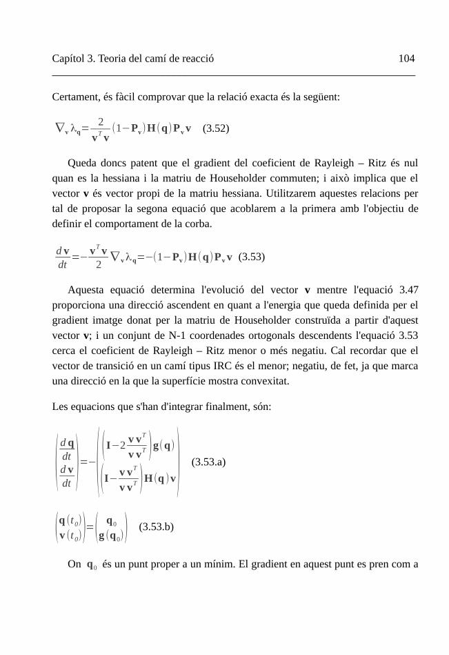
Capítol 3. Teoria del camí de reacció 104 __________________________________________________________________
Certament, és fàcil comprovar que la relació exacta és la següent:
∇v λq=2
vT v(1−Pv)H(q)Pv v (3.52)
Queda doncs patent que el gradient del coeficient de Rayleigh – Ritz és nul quan es la hessiana i la matriu de Householder commuten; i això implica que el vector v és vector propi de la matriu hessiana. Utilitzarem aquestes relacions per tal de proposar la segona equació que acoblarem a la primera amb l'objectiu de definir el comportament de la corba.
d vdt=−
vT v2∇ vλq=−(1−Pv)H(q)Pv v (3.53)
Aquesta equació determina l'evolució del vector v mentre l'equació 3.47 proporciona una direcció ascendent en quant a l'energia que queda definida per el gradient imatge donat per la matriu de Householder construïda a partir d'aquest vector v; i un conjunt de N-1 coordenades ortogonals descendents l'equació 3.53 cerca el coeficient de Rayleigh – Ritz menor o més negatiu. Cal recordar que el vector de transició en un camí tipus IRC és el menor; negatiu, de fet, ja que marca una direcció en la que la superfície mostra convexitat.
Les equacions que s'han d'integrar finalment, són:
(d qdtd vdt)=−( (
I−2v vT
v vT )g(q)
(I−v vT
v vT )H(q )v) (3.53.a)
(q (t 0)
v (t 0))=(q0
g (q0)) (3.53.b)
On q0 és un punt proper a un mínim. El gradient en aquest punt es pren com a

De la superfície d'energia potencial a la reactivitat química 105 __________________________________________________________________
vector v. Aquestes foren les equacions proposades per E i Zhou de les quals se n'ha proporcionat una aproximació diferent20.
IV.2 Comportament i anàlisi
El mètode d'integració emprat és el Runge-Kutta d'ordre 8(5,3)25. Hem emprat tres superfícies analítiques bidimensionals per tal d'analitzar el comportament del mètode.
Superfície Wolfe-Quapp
Figura 3.9a: Comportament del mètode a la superfície Wolfe – Quapp. La corba comença al punt (1.2,-1.5) a les rodalies d'un mínim. Acaba a prop de l'estat de transició ubicat a (0.093, 0.174). El vector v a cada punt està representat mitjançant una fletxa. Es pot observar com, inicialment, aquest vector coincideix amb el gradient (és ortogonal a les línies de contorn); al final, coincideix amb el vector de transició del punt de sella, que és el vector que té com a direcció el vector propi associat al valor propi negatiu de la hessiana en aquell punt: es constata com les N darreres equacions (3.53a) minimitza el valor del coeficient de Rayleigh – Ritz (3.51).

Capítol 3. Teoria del camí de reacció 106 __________________________________________________________________
L'equació que defineix aquesta superfície és la següent26,27:
V (x , y )=x4+ y 4
−2 x2−4 y2
+xy+0.3 x+0.1 y (3.54)
El punt on comença la dinàmica és a les rodalies del mínim ubicat a (1.124,-1.486) amb energia -6.369 (unitats arbitràries). Es tria el punt (1.2,-1.5) i s'hi associa com a vector v inicial el gradient. A les figura 3.9 i 3.10 es pot observar com la corba arriba exitosament a l'estat de transició ubicat a (0.093, 0.174) amb energia -0.644.
Figura 3.9b: Representació tridimensional de la superfície Wolfe – Quapp amb aquesta primera corba representada sobre ella.
Figura 3.10a: Representació tridimensional de la trajectòria sobre la superfície Wolfe – Quapp.

De la superfície d'energia potencial a la reactivitat química 107 __________________________________________________________________
La següent corba està representada a les figures 3.10 i arriba al mateix estat de transició revelant noves característiques del mètode. En aquest cas, la corba comença a prop d'un mínim ubicat a (-1.174,1477) amb energia -6.762. El vector v pren inicialment el valor del gradient i evoluciona d'acord amb les equacions (3.53a) . El camí ascendeix fins a un cert valor on l'energia és màxima respecte a la resta de la corba; allà trobem un punt de retorn i la trajectòria descendeix cap al punt de sella ubicat a (0.093,0.174) amb energia 0.644. Quan ho fa, es pot observar com el vector v va adoptant progressivament la direcció del vector de transició al punt de sella.
Respecte al punt de retorn esmentat, cal definir i caracteritzar ben bé aquest
Figura 3.10b: Comportament del mètode presentat sobre la superfície Wolfe – Quapp. El vector v hi apareix reflectit mitjançant fletxes. Es pot observar com inicialment la tangent de la corba pràcticament coincideix amb el gradient: és el tipus de tangent que hom espera trobar en un IRC. No obstant, després trobem un tipus de comportament comprensible mitjançant les relacions entre els vectors involucrats tal i com es descriu al text.

Capítol 3. Teoria del camí de reacció 108 __________________________________________________________________
punt. En primer lloc, no és característic de la superfície d'energia potencial sinó de la corba. Aquest punt representa un canvi de direcció del camí que es defineix com aquell punt en el que la corba no creua una línia de contorn sinó que la toca tangencialment; matemàticament es caracteritza com el punt en el que la variació del potencial respecte t es torna nul·la i per tant el gradient i la tangent són ortogonals. En el nostre cas podem desenvolupar aquesta equació per obtenir-ne més informació:
dVdt=gT dq
dt=−gT Uv g=−gT
(I−Pv)g+gT Pv g=0 (3.55)
D'aquí deduïm que en el context d'aquest mètode un punt de retorn apareix quan es satisfà la igualtat:
gT(I−Pv)g=gT Pv g (3.56)
És a dir, hi ha una igualtat entre el quadrat de la norma del gradient projectada en el subespai definit per v i en el seu espai complementari. Desenvolupant aquest
resultat i tenint en compte la definició de Pv es pot arribar a
1/21/2=gT v /(gT g vT g )1/2 ; per tant, és general que en un punt de retorn l'angle
entre el gradient i el vector v és de 45º. Anàlogament, es pot establir el que succeeix per a una energia creixent o decreixent: correspondran a un angle entre g i v de menys de 45º o de més de 45º, respectivament. Lògicament, la variació d'aquest angle és contínua i trobem sempre un punt on l'angle és exactament 45º: el punt de retorn és un cas especial d'aquesta última situació.
Recapitulant, el comportament del mètode ve donat per la relació entre tres vectors: el vector tangent a la corba, el vector gradient i el vector v que en tot moment varia seguint les N darreres equacions 3.53a. Aquest vector té associat un
quocient de Rayleigh – Ritz que sempre està entre els valors λn≥λv≥λm on
λn i λm són els valors propis més gran i més petit de la hessiana en el punt
considerat, respectivament. A l'estat de transició λv=λm .
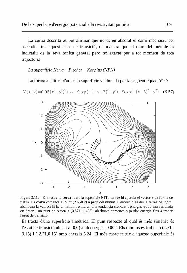
De la superfície d'energia potencial a la reactivitat química 109 __________________________________________________________________
La corba descrita es pot afirmar que no és en absolut el camí més suau per ascendir fins aquest estat de transició, de manera que el nom del mètode és indicatiu de la seva tònica general però no exacte per a tot moment de tota trajectòria.
La superfície Neria – Fischer – Karplus (NFK)
La forma analítica d'aquesta superfície ve donada per la següent equació28,29:
V (x , y )=0.06 (x2+ y2
)2+ xy−9exp (−(−x−3)2− y2
)−9exp(−(x+3)2− y2) (3.57)
Es tracta d'una superfície simètrica. El punt respecte al qual és més simètric és l'estat de transició ubicat a (0,0) amb energia -0.002. Els mínims es troben a (2.71,-0.15) i (-2.71,0.15) amb energia 5.24. El més característic d'aquesta superfície és
Figura 3.11a: Es mostra la corba sobre la superfície NFK; també hi apareix el vector v en forma de fletxa. La corba comença al punt (2.6,-0.2) a prop del mínim. L'evolució es duu a terme pel gorg; abandona la vall on hi ha el mínim i entra en una tendència creixent d'energia, troba una serralada on descriu un punt de retorn a (0,871,-1.428); aleshores comença a perdre energia fins a trobar l'estat de transició.

Capítol 3. Teoria del camí de reacció 110 __________________________________________________________________
l'existència de gorgs a prop dels punts (-2,2) i (2,-2); el gorg és les parts més estretes d'una vall, o, dit d'una altra manera, un gorg és la part d'una vall on les parets d'aquesta vall són més a prop. A les figures 3.11 s'observa com una
Figura 3.11b: Representació tridimensional de la corba sobre la superfície NFK.
Figura 3.12a:Trajectòria sobre la superfície NFK. Les fletxes indiquen la direcció del vector v a cada punt. La corba comença al punt (2.8,0.0) i ascendeix en energia fins a trobar un punt de retorn. Aleshores comença el descens fins a localitzar el punt de sella. Si la comparem amb la corba anterior a la mateixa superfície, la diferència en el seu comportament és que l'estructura de les equacions obliguen a la trajectòria a seguir el gorg en el cas representat a la figura 3.11.

De la superfície d'energia potencial a la reactivitat química 111 __________________________________________________________________
trajectòria que tingui com a punt inicial un punt situat entre el mínim i el gorg emprendrà el camí de la vall per finalment localitzar l'estat de transició.
A les figures 3.12 s'observa una trajectòria que té com a punt inicial un punt que es proper al mínim però no és entre el gorg i el mínim. La trajectòria troba un altre camí per tal d'arribar al punt de sella.
Superfície Müller – Brown
Aquesta superfície3, que s'ha emprat anteriorment per tal d'introduir aquest capítol, mostra els límits del present mètode. Té un mínim a prop del qual es comença la trajectòria situat en una vall molt profunda, concretament a les coordenades (-0.558,1.442). El que s'observa és que la trajectòria surt fora de la part de la superfície que s'utilitza per tal de representar problemes químics i troba el punt de retorn relativament lluny. Aquesta zona es caracteritza per tenir una estructura diferent de la trobada en els anteriors exemples: no hi ha proximitat a cap línia límit vall – serralada. Degut a això, la corba no pot trobar el vector v adient per començar el descens cap a la vall; tot i així, després d'escombrar gran part de la
Figura 3.12b: Representació de la trajectòria sobre la superfície NFK.

Capítol 3. Teoria del camí de reacció 112 __________________________________________________________________
superfície, acaba trobant el vector v que la conduirà fins a l'estat de transició. Tot això s'il·lustra a la figura 3.13.
IV.3. Generalització de la teoria a punts de sella d'ordre N
Les equacions presentades fins ara són vàlides per a la cerca d'un punt de sella d'ordre 1 però són fàcilment generalitzables:
Si J és l'ordre del punt de sella que es vol localitzar, on J≤N , les equacions 3.53 prenen la següent forma:
Figura 3.13: Cerca de l'estat de transició mitjançant el mètode de l'ascens gradual a la superfície Müller – Brown. La trajectòria comença al punt (-0.558,1.442), mostra el comportament caòtic descrit al text i finalment troba l'estat de transició a (-0.822,0.624).
De la superfície d'energia potencial a la reactivitat química 113 __________________________________________________________________
(dqdt
d v1
dt⋮
d vJ
dt
)=−((I−2∑
i=1
J
Pvi)g (q )
(I−∑i=1
J
Pvi)H(q)v1+( ∑i=1∀ i≠1
J
Pvi)H(q)v1
⋮
(I−∑i=1
J
Pv i)H(q )vJ+( ∑i=1∀ i≠J
J
Pvi)H(q)vJ
) (3.58.a)
amb les condicions inicials:
(q( t0)
v1(t 0)⋮
vJ (t 0))=(
q0
g (q0)⋮
p0J ) (3.58.b)
on Pvi=v i v i
T/(vi
T v i) per a i=1,...,J; i { P0i }i=2
J és un conjunt de J-1 vectors
ortogonals entre ells i ortogonals amb el vector gradient g (q0) . En el cas de que
J=N aleshores la matriu identitat a l'equació 3.58.a hauria de ser substituïda per la resolució de la identitat:
I=∑i=1
N
Pvi (3.59)
La variació de l'energia en aquesta corba vindria donada per:
dVdt=−gT d q
dt=−gT (I−2∑
i=1
J
Pvi)g (q )=2(∑i=1
J (gT v i )2
gT g v iT v i
−12 )gT g (3.60)
Aquesta equació ens diu que quan la suma del quadrat dels components del
vector gradient projectat al subespai dels vectors vi és major que 1/2 la corba és
creixent en energia; si és menor que 1/2 aleshores és decreixent. Si el resultat és
Capítol 3. Teoria del camí de reacció 114 __________________________________________________________________
exactament 1/2 som a un punt de retorn.
V. Trajectòries newtonianes
V.1. Fonamentació matemàtica de les trajectòries newtonianes
Les trajectòries newtonianes, també anomenades seguiment del gradient reduïth, són un tipus de corba caracteritzats pel fet de que a cada punt de la corba el vector gradient conserva sempre la mateixa direcció. La naturalesa variacional d'aquesta corba ha estat demostrada30 i el fet de que se l'anomeni d'una o una altra manera ve donada pel mètode emprat per integrar-les.
Una trajectòria newtoniana es pot integrar pel mètode d'Euler – Branin. En aquest cas, la tangent ve donada de forma explícita per
dq (t)dt
=±A (q (t))g(q (t )) (3.61)
on A és la matriu adjunta de la hessiana.
Una altra manera de definir i caracteritzar aquestes corbes és a partir del
projector Qr=1−Pr on, igual que en el cas dels capítols anteriors:
Pr=r rT
rT r (3.62)
La condició que en tot moment s'hauria de complir és l'equació de projecció. Aquí, r és la direcció arbitrària que haurà de ser igual al gradient durant tota la corba:
Qr g (q (t))=0 (3.63)
h De l'anglés Reduced Gradient Following, RGF.

De la superfície d'energia potencial a la reactivitat química 115 __________________________________________________________________
No obstant, aquesta segona possibilitat dificulta el fet de trobar la tangent que s'ha de buscar numèricament31 o emprant un desenvolupament pertorbacional semblant al proposat al capítol anterior.
Una manera de relacionar ambdues equacions és la que es proposa a continuació. Si derivem l'expressió 3.63 respecte a t obtenim:
Qr Hd qdt=O (3.64)
on hem aplicat la derivada direccional d /dt=(dq /dt)T∇ q . Aquest és un
sistema de N-1 equacions si N és la dimensió del problema. Les equacions 3.63 i 3.64 es poden relacionar mitjançant la variació del gradient sobre la corba:
d g /dt=det(H)g , on s'ha emprat que AH=det(H) . Si g té la direcció del vector
r, aquesta darrera expressió ens indica que la seva variació també es produeix en aquella direcció; per tant, l'expressió d'Euler – Branin preserva la direció del gradient igual que succeeix amb l'equació 3.63. Podem concloure que ambdues equacions són dues formes matemàtiques diferents de tractar el mateix mètode de les trajectòries de Newton o RGF.
Qualsevol punt estacionari pot ser un atractor de trajectòries newtonianes depenent de l'índex del punt estacionari i el signe de l'equació 3.6131,32,33. Si el signe de l'equació 3.61 és positiu i el nombre de valors propis de la hessiana és senar aleshores es pot demostrar que les trajectòries newtonianes són atretes per aquest punt; si el nombre de valors propis és parell, en canvi, les trajectòries són repel·lides. Si el signe de l'equació 3.61 és negatiu passa el contrari. Per exemple, un punt de sella d'ordre 2 serà atractor de trajectòries de Newton si el signe de l'equació és negatiu. Això es mostra a la figura 3.14 a l'esquerra. Aquesta figura
respon a l'equació −x2−5y2 . Un altre exemple d'un atractor el trobem en una
superfície en forma d'embut ubicat a la dreta de la figura 3.14. L'equació que hi
correspon és −√x2+5y2 .
Aquestes propietats matemàtiques fan que les trajectòries newtonianes siguin

Capítol 3. Teoria del camí de reacció 116 __________________________________________________________________
un tipus de corba idònia per tal d'explorar superfícies d'energia potencial tot localitzant estructures topològicament rellevants.
V.2 Les interseccions còniques com a atractores de les trajectòries newtonianes34
En el context de l'aproximació Born-Oppenheimer, a cada posició q donada dels nuclis hi correspon un i només un valor d'energia potencial V(q) per a una simetria d'espai i d'espín donada. Com s'ha descrit ja anteriorment al capítol 2,cada estat dóna lloc a una hipersuperfíce. Per tal d'explicar intuïtivament quan és vàlida aquesta aproximació, hom sol referir-se a la velocitat relativa entre els electrons i els nuclis: si es pot considerar que per a una variació donada de posició dels nuclis els electrons es recol·loquen instantàniament, aleshores l'aproximació serà vàlida. A mesura que aquesta condició deixa de complir-se, l'aproximació anirà fallant amb conseqüències evidents sobre les prediccions realitzades emprant el model Born – Oppenheimer. El fet és que aquesta aproximació és acceptable per tal de descriure sistemes moleculars a prop de l'equilibri (entenent com a 'descripció acceptable' una descripció que permeti predir amb precisió les propietats del
Figura 3.14: A l'esquerra es mostra la projecció d'un punt de sella d'ordre 2 en les dimensions en les quals és màxim. A la dreta una superfície en forma d'embut. A la part superior es mostra una representació tridimensional d'ambdues superfícies. A la part inferior una projecció bidimensional acompanyada del camp vectorial Ag que permet apreciar que són similars en quant a la capacitat d'atraure trajectòries newtonianes.

De la superfície d'energia potencial a la reactivitat química 117 __________________________________________________________________
sistema).
Un punt d'una intersecció cònica és un punt on es dóna la confluència de dues hipersuperfícies associades a estats electrònics de la mateixa multiplicitat d'espín. La topologia d'aquesta confluència és la d'un doble con o diabolo35. De vegades aquests punts també són anomenats punts diabòlics. Cal destacar que altres tipus d'interseccions són possibles36.
Els efectes d'una intersecció cònica poden ser molt importants. Hom36 els classifica en directes (com la desexcitació sense radiació / excitació sense absorció i el recreuament no adiabàtic) i indirectes (la fase geomètrica o fase de Berry). La importància de les interseccions còniques ha estat reconeguda des de fa dècades en sistemes petits i grans (biològics) (veure referències a la introducció de la referència 36). Per tant, la localització d'interseccions còniques ha bastit una col·lecció bibliogràfica generosa 37,38,39.
Com s'ha esmentat anteriorment, la topologia d'una intersecció cònica és la pròpia d'un embut o con des del punt de vista de la superfície que rau a energia inferior. I, tal i com s'ha argumentat anteriorment també, aquesta mena de forma actua com a atractora de trajectòries newtonianes; per tant, es proposa utilitzar aquesta mena de corba com a mètode per a localitzar interseccions còniques. Tal i com es pot veure a la figura 3.16 és possible partir de punts de sella o mínims per anar a parar a la intersecció cònica en qüestió marcada com a CI. Topològicament,
Figura 3.15: Representació tridimensional esquemàtica d'una intersecció cònica. En un cas com aquest en el que la intersecció cònica té lloc a un espai bidimensional parlem de punts (n-2) d'intersecció cònica.
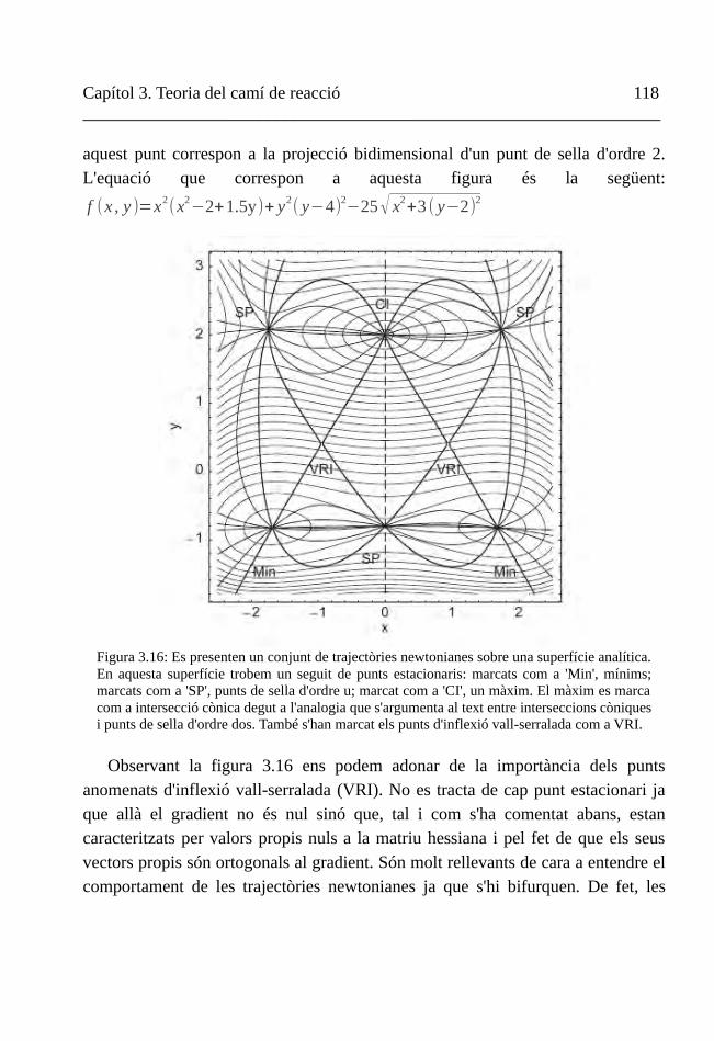
Capítol 3. Teoria del camí de reacció 118 __________________________________________________________________
aquest punt correspon a la projecció bidimensional d'un punt de sella d'ordre 2. L'equació que correspon a aquesta figura és la següent:
f (x , y )=x2(x2−2+1.5y)+ y2
( y−4)2−25√ x2+3 ( y−2)2
Observant la figura 3.16 ens podem adonar de la importància dels punts anomenats d'inflexió vall-serralada (VRI). No es tracta de cap punt estacionari ja que allà el gradient no és nul sinó que, tal i com s'ha comentat abans, estan caracteritzats per valors propis nuls a la matriu hessiana i pel fet de que els seus vectors propis són ortogonals al gradient. Són molt rellevants de cara a entendre el comportament de les trajectòries newtonianes ja que s'hi bifurquen. De fet, les
Figura 3.16: Es presenten un conjunt de trajectòries newtonianes sobre una superfície analítica. En aquesta superfície trobem un seguit de punts estacionaris: marcats com a 'Min', mínims; marcats com a 'SP', punts de sella d'ordre u; marcat com a 'CI', un màxim. El màxim es marca com a intersecció cònica degut a l'analogia que s'argumenta al text entre interseccions còniques i punts de sella d'ordre dos. També s'han marcat els punts d'inflexió vall-serralada com a VRI.
De la superfície d'energia potencial a la reactivitat química 119 __________________________________________________________________
trajectòries newtonianes també s'utilitzen per tal de localitzar aquesta mena de punts.40
És important raonar fins a quin punt són equivalents els punts de sella i les interseccions còniques, que topològicament es comporten com embuts.
La primera gran diferència és el gradient. El punt de la intersecció cònica – (0,0) a la figura 3.14 – és un punt estacionari en el cas d'un màxim però no en el cas d'un embut.
En segon lloc també trobarem diferències en la matriu hessiana. En una intersecció cònica els valors propis de la hessiana són indeterminats. En el cas de l'embut els valors propis tenen una expressió analítica però són també problemàtics: un es manté 0 i l'altre esdevé menys infinit. En el cas del màxim (punt de sella d'ordre 2) no es dóna cap d'aquestes circumstàncies especials respecte de la curvatura. Aquest fet és molt útil de cara a detectar la proximitat
d'una intersecció cònica. Integrant l'equació 1, es troba que el valor ∣Ag∣ creix
molt. Això és degut a que els valors propis μ de la matriu A estan relacionats amb
els λ de la hessiana. Concretament, μi=∏j≠i
n
λ j.
De cara a implementar aquest mètode com a localitzador d'interseccions còniques en un sistema químic és esperable que apareguin dificultats tècniques que no hi són quan el mètode es proba sobre superfícies analítiques com en el cas de la figura 3.16. A les rodalies d'una intersecció cònica, el mètode Newton-Raphson de predicció i correcció sovint falla en l'etapa de correcció si s'empra la derivació de l'equació 3.62. En el càlcul de les trajectòries subsegüents s'ha treballat amb el predictor emprant l'equació 3.61; el fet d'emprar aquesta tècnica fa que hi pugui haver lleus diferències respecte de les trajectòries integrades utilitzant el predictor corrector i per aquest motiu a aquestes trajectòries se les anomena quasi-newtonianes. En els següent apartat aquesta denominació quedarà sobreentesa.

Capítol 3. Teoria del camí de reacció 120 __________________________________________________________________
V.3 El cas del radical al·lil
El tancament del radical ciclopropil, que té un nombre senar d'electrons, està prohibit per les regles de Woodward-Hofmann que són les regles que prediuen el comportament conrotatori o disrotatori depenent de la naturalesa orbital d'un sistema donat41. No obstant, aquest tancament s'observa a nivell experimental tant per activació tèrmica com per activació fotoquímica. A la bibliografia podem trobar treballs sobre la localització d'interseccions còniques en aquest sistema42.
S'han definit les distàncies sobre el radical al·lil com es mostra a la taula següent i a la figura 3.17:
c1
c2 1 r1
c3 1 r2 2 c2c1c3
h4 1 hc1 2 hcc1 3 dih1
h5 2 hc2 1 hcc2 3 dih2
h6 3 hc3 1 hcc3 2 dih3
h7 2 hc4 1 hcc4 3 dih4
h8 3 hc5 1 hcc5 2 dih5
Per tal de dur a terme els càlculs s'ha emprat el programa GAMESS-US43 amb el mètode CASSCF(3,3) i la base 6-31G(d,p). S'ha utilitzat un programa que integra les trajectòries newtonianes de manera acoblada a l'execució de GAMESS-US. Aquest programa està disponible a http://www.math.uni-leipzig.de/~quapp/SkewVRIs.html. En tot moment es tenen en compte les 3N-6=18 coordenades del sistema.
És convenient destacar que per a aquest sistema concret ha estat impossible dur a terme una representació del potencial en funció de dues coordenades (o combinació lineal d'elles) que sigui fàcilment entenedora i sobre la qual es puguin
Figura3.17: Radical al·lil i coordenades.
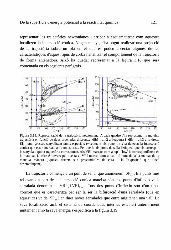
De la superfície d'energia potencial a la reactivitat química 121 __________________________________________________________________
representar les trajectòries newtonianes i arribar a esquematitzar com aquestes localitzen la intersecció cònica. Nogensmenys, s'ha pogut realitzar una projecció de la trajectòria sobre un pla en el que es poden apreciar algunes de les característiques d'aquest tipus de corba i analitzar el comportament de la trajectòria de forma entenedora. Això ha quedat representat a la figura 3.18 que serà comentada en els següents paràgrafs.
La trajectòria comença a un punt de sella, que anomenem SPaa . Els punts més
rellevants a part de la intersecció cònica mateixa són dos punts d'inflexió vall-
serralada denominats VRIup i VRIlow . Tots dos punts d'inflexió són d'un tipus
concret que es caracteritza per ser la ser la bifurcació d'una serralada (que en
aquest cas ve de SPaa ) en dues noves serralades que entre mig tenen una vall. La
seva localització amb el sistema de coordenades internes establert anteriorment juntament amb la seva energia s'especifica a la figura 3.19.
Figura 3.18: Representació de la trajectòria newtoniana. A cada quadre s'ha representat la mateixa trajectòria en funció de dues ordenades diferents: -dih5 i dih2 a l'equerra i -dih4 i dih3 a la dreta. Els punts grossos senyalitzen punts especials exceptuant els punts on s'ha detectat la intersecció cònica que estan marcats amb un asterisc. Pel que fa als punts de sella l'etiqueta que els correspon ja senyala a quina trajectòria corresponen. Als VRI marcats com a 'up' i 'low' la correspondència és la mateixa. L'ordre és invers pel que fa al VRI marcat com a 'ca' i al punt de sella marcat de la mateixa manera (aquests darrers són prescindibles de cara a la l'exposició que s'està desenvolupant).

Capítol 3. Teoria del camí de reacció 122 __________________________________________________________________
De cada punt d'inflexió vall-serralada emergeixen 4 trajectòries. Hom tendeix a nomenar-ne dues 'laterals' i a dues 'centrals', sent més o menys clar quina és cadascuna depenent de l'ocasió. En el nostre cas i particularment a la part inferior de la gràfica esquerra i la superior de la dreta de la figura 3.18 la nomenclatura és prou entenedora.
De les quatre trajectòries que surten del VRIlow , les dues laterals van
directament a parar a la intersecció cònica. Pel que fa a les centrals, una finalitza a
la vall a la que arriba a través del punt de sella SPaa i la segona acaba al VRIup .
De les tres restants d'aquest segon punt d'inflexió vall-serralada, la segona branca central va directament a la intersecció cònica. Les dues laterals acaben una al punt d'inflexió després de descriure cercles mentre que la segona acaba a una zona de serralades de la superfície.
Amb l'objectiu de verificar la qualitat dels punts identificats com a part de la intersecció cònica s'ha dut a terme un càlcul CASCI per trobar la diferència d'energia entre l'estat fonamental i els dos primers estats excitats en aquest punt. És un càlcul basat en els orbitals naturals del CAS(3,3) (quartet). Trobem que la diferència d'energia entre els dos doblets és de 0.5 kcal/mol i considerem per tant que la degeneració dels dos estats en aquest punt és prou accentuada com per a considerar que la cerca ha estat un èxit.
Figura 3.19: Localització i energia dels punts d'inflexió vall-serralada (VRI) més rellevants i de la intersecció cònica presents a la figura 3.18.

De la superfície d'energia potencial a la reactivitat química 123 __________________________________________________________________
VI. Conclusions
La sinergia de vàries disciplines, especialment les matemàtiques pel que fa al càlcul de variacions o el mètode de característiques; la mecànica clàssica pel que fa a la mecànica Lagrangiana o el principi de Fermat – Huygens; i la química pel que fa a la perspectiva de tot desenvolupament enfocada sempre a resoldre problemes químics, permet bastir diferents aproximacions a la teoria del camí de reacció.
En el present capítol se n'ha tractat una sèrie d'exemples buscant, quan ha estat possible, partir de principis comuns. S'ha arribat a diferents camins de reacció amb les seves virtuts i defectes; aquests camins són models que ajuden a la comprensió de visions abstractes de problemes físicoquímics – com és la síntesi de l'essència d'una superfície d'energia potencial N dimensional en una sola corba – o, al contrari, models que busquen reconciliar fenòmens experimentals amb models abstractes quan la connexió es torna difusa – com es pot veure al final de la secció que tracta els gradients extremals –.
La conveniència d'utilitzar un model de camí de reacció va lligada al diagrama de flux exposat al capítol I: és una eina metodològica que ha de resoldre un determinat problema. I el podem donar per resolt depenent de l'enfocament que n'hagem fet. El fet de que el camí de reacció redueix les N dimensions d'una hipersuperfície a una de sola es pot entendre com un reduccionisme que fa perdre informació; però no oblidem el fet de que l'objectiu final de qualsevol estudi acadèmic és la resolució d'un problema a través del coneixement que proporciona un model determinat i això implica manegar quantitats d'informació possibles d'assimilar. Tard o d'hora, sigui quin sigui el volum de la informació que a priori siguem capaços de generar, l'haurem de reduir mitjançant un model justificable a un volum tal que sigui factible de processar i entendre mitjançant l'intel·lecte humà.
Capítol 3. Teoria del camí de reacció 124 __________________________________________________________________
Bibliografia
1. D. Heidrich i W. Quapp, Theoretica Chimica Acta, 70, 89 (1986)2. R. Minyaev, I. Getmanskii i W. Quapp, Russian Journal of Physical Chemistry, 78, 1494 (2004)3. K. Müller i L. D. Brown, Theoretica Chimica Acta, 53, 75 (1979)4. K. Fukui, The Journal of Physical Chemistry, 74, 4161 (1970)5. R. Crehuet i J. M. Bofill, The Journal of Chemical Physics, 122, 234105 (2005)6. J. M. Bofill, W. Quapp i M. Caballero, Journal of Chemical Theory and Computation, 8, 4856 (2012)7. A. Aguilar-Mogas, X. Gimenez i J. M. Bofill, The Journal of Chemical Physics, 128, 104102 (2008)8. R. Courant i D. Hilbert. Methods of Mathematical Physics, Part 2. Wiley (1953)9. A. Aguilar-Mogas, R. Crehuet, X. Giménez i J. M. Bofill, Molecular Physics, 105, 2475 (2007)10. M. Llunell, P. Alemany i J. Bofill, Theoretical Chemistry Accounts, 121, 279 (2008)11. C. Huygens. Traité de la Lumière. (1690)12. D. Hoffman, R. Nord i K. Ruedenberg, Theoretica Chimica Acta, 69, 265 (1986)13. W. Quapp, Theoretica Chimica Acta, 75, 447 (1989)14. J. M. Bofill, W. Quapp i M. Caballero, Journal of Chemical Theory and Computation, 8, 927 (2012)15. R. McWeeny, Phys. Rev., 126, 1028 (1962)16. J. Sun i K. Ruedenberg, The Journal of Chemical Physics, 98, 9707 (1993)17. P. Valtazanos i K. Ruedenberg, Theoretica Chimica Acta, 69, 281 (1986)18. W. H. Press, S. A. Teukolsky, W. T. Vetterling i B. P. Flannery. Numerical Recipes in Fortran 77 The Art of Scientific Computing. Press Syndicate of the University of Cambfidge (1997)19. G. A. Worth, M. H. Beck, A. Jäckle i H. Meyer, The MCTDH Package, Version 8.2,(2000), University of Heidelberg, Heidelberg, Germany. H.-D. Meyer, Version 8.3 (2002),Version 8.4 (2007). See http://mctdh.uni-hd.de20. W. E i X. Zhou, Nonlinearity, 24, 1831 (2011)21. C. M. Smith, Theoretica Chimica Acta, 74, 85 (1988)22. C. M. Smith, International Journal of Quantum Chemistry, 37, 773 (1990)23. J. Sun i K. Ruedenberg, The Journal of Chemical Physics, 101, 2157 (1994)

De la superfície d'energia potencial a la reactivitat química 125 __________________________________________________________________
24. A. S. Householder, Journal of the ACM, 5, 339 (1958)25. E. Hairer, S. P. Norsett i G. Wanner. Solving Ordinary Differential Equations I Nonstiff Problems. Springer-Verlag, Springer Series in Computational Mathematics, Second Edition (1993)26. S. Wolfe, H. B. Schlegel, I. G. Csizmadia i F. Bernardi, Journal of the American Chemical Society, 97, 2020 (1975)27. W. Quapp, The Journal of Chemical Physics, 122, 174106 (2005)28. M. Hirsch i W. Quapp, Journal of Mathematical Chemistry, 36, 307 (2004)29. E. Neria, S. Fischer i M. Karplus, The Journal of Chemical Physics, 105, 1902 (1996)30. J. M. Bofill i W. Quapp, The Journal of Chemical Physics, 134, 074101 (2011)31. W. Quapp, M. Hirsch, O. Imig i D. Heidrich, Journal of Computational Chemistry, 19, 1087 (1998)32. M. Hirsch i W. Quapp, Journal of Mathematical Chemistry, 36, 307 (2004)33. W. Quapp, M. Hirsch i D. Heidrich, Theoretical Chemistry Accounts, 100, 285 (1998)34. W. Quapp, J. M. Bofill i M. Caballero, Chemical Physics Letters, 541, 122 (2012)35. M. Berry i M. Wilkinson, Proceedings of the Royal Society of London Series A-MathematicalPhysical and Engineerings Sciences, 392, 15 (1984)36. D. R. Yarkony, Reviews of Modern Physics, 68, 985 (1996)37. J. Anglada i J. Bofill, Journal of Computational Chemistry, 18, 992 (1997)38. F. Sicilia, L. Blancafort, M. J. Bearpark i M. A. Robb, Journal of Chemical Theory and Computation, 4, 257 (2008)39. S. Maeda, K. Ohno i K. Morokuma, Journal of Chemical Theory and Computation, 6, 1538 (2010)40. W. Quapp i B. Schmidt, Theoretical Chemistry Accounts, 128, 47 (2011)41. R. B. Woodward i R. Hoffmann, Journal of the American Chemical Society, 87, 395 (1965)42. Y. Haas, S. Cogan i S. Zilberg, International Journal of Quantum Chemistry, 102, 961 (2005)43. M. W. Schmidt, K. K. Baldridge, J. A. Boatz, S. T. Elbert, M. S. Gordon, J. H. Jensen, S. Koseki, N. Matsunaga, K. A. Nguyen, S. Su, T. L. Windus, M. Dupuis i J. A. Montgomery, Journal of Computational Chemistry, 14, 1347 (1993)

Capítol 4
Dinàmica
Fotografia d'una peça de l'escultor Giacometti amb cc by -nc -sa 3.0 es de la pàgina web http://madridfree.com/giacometti-terrenos-de-juego-exposicion/

Capítol 4. Dinàmica 127__________________________________________________________________
I. Dinàmica quàntica
I.1 Paquets d'ones1
És habitual escriure l'equació de Schrödinger dependent del temps separant la
funció d'ona en un terme espacial i un de temporal: Ψ(x , t)=ψ(x)χ (t) :
Si l'equació de Schrödinger dependent del temps s'escriu:
i ℏ ∂∂ t
Ψ(x , t)=HΨ(x , t ) (4.1)
i es substitueix la consideració anterior sobre la separabilitat, s'obté:
i ℏ χ (t)χ (t)−1=H ψ(x )ψ(x)−1 (4.2)
on s'ha separat l'equació en una part dependent del temps -esquerra- i una part dependent de la posició -dreta-.
Ambdues parts han de ser iguals a una constant, E (energia). Així, s'obtenen dues equacions, una per a la part dependent del temps i una altra per a la part dependent de la posició:
i ℏ χ(t)=Eχ (t) (4.3a )
H ψE(x)={−ℏ2
2m∂
2
∂ x2 +V (x)}ψE (x)=EψE(x) (4.3b)
La solució de l'equació diferencial 4.3a és:
χ (t)=χ0e−iℏ
E t(4.4)
L'equació 4.3b és l'equació de Schrödinger independent del temps i depèn específicament del potencial. A la majoria de casos, aquesta equació no es pot
Capítol 4. Dinàmica 128__________________________________________________________________
resoldre analíticament. És possible aleshores escriure una solució de l'equació de Schrödinger dependent del temps com a:
Ψ(x ,t)=ψE(x) χ0 e−iℏ
Et (4.5)
on χ0 és un factor que podria haver estat inclòs perfectament dins de ψE(x). La magnitud d'aquest darrer terme està determinada per l'equació de Schrödinger independent del temps; es pot escollir – incloent el factor d'integració χ0 – de tal manera que es compleixi la condició de normalització,
∫−∞
∞
∣Ψ(x ,t )∣2d x=1 (4.6)
i així escriure sense pèrdua de generalitat:
Ψ(x ,t)=ψE(x)e−iℏ
Et (4.7)
L'equació 4.7 té una dependència temporal trivial. Si es considera la densitat de
probabilitat ∣Ψ(x ,t )∣2 , determinada per l'equació 4.7, s'obté:
∣Ψ(x ,t )∣2=(ψE(x)e−iℏ
E t)
*ψE(x)e
−iℏ
E t=∣ΨE(x)∣
2 (4.8)
que és una equació independent del temps. Si la densitat de probabilitat no varia amb el temps, no hi ha dependència temporal en quant a la situació de la partícula – no hi ha moviment efectiu. Ara bé, la mecànica quàntica ha de ser capaç de descriure moviment, ja que el món microscòpic està sotmès a canvi i variacions constants. La resolució a aquesta aparent paradoxa rau en el fet de que l'equació 4.5 no és més que una solució particular de l'equació diferencial que és l'equació de Schrödinger dependent del temps. Per formular una solució general a aquesta equació, es pot emprar una combinació lineal de dues solucions particulars – en el cas més simple possible – , cadascuna amb la seva fase dependent del temps:
Capítol 4. Dinàmica 129__________________________________________________________________
Ψ(x ,t)=aψE(x )e−iℏ
E t+bψE' (x)e
−iℏ
E' t (4.9)
Ara la densitat de probabilitat dependrà del temps:
∣Ψ(x ,t )∣2=∣a∣2∣ψE(x)∣2+∣b∣2∣ψE ' (x)∣
2+2Re {a*bψE* (x)ψE ' (x)e
−i(E '−E ) t
ℏ } (4.10)
A l'equació 4.10 s'hi distingeixen tres termes: un que correspon a ψE, un altre que correspon a ψE' i un darrer que correspon a la interferència d'ambdós. Aquest terme d'interferència és el resultat de la superposició d'estats propis amb diferents energies: és el que s'anomena paquet d'ones. Tota la dependència temporal de
∣Ψ(x ,t )∣2 queda continguda dins d'aquest terme d'interferència i d'aquesta manera
és remarcable que, generalment, un paquet d'ones – una superposició d'estats que tenen diferents energies – és necessari per tal de modelitzar la dependència temporal de la probabilitat i altres quantitats observables, tal com la posició mitjana i el moment mig d'una partícula.
Es pot escriure la solució general de l'equació de Schrödinger dependent del temps generalitzant el màxim possible mitjançant un sumatori estès des de n=1 fins a infinit:
Ψ(x ,t)=∑n=1
∞
an ψn(x)e−iℏ
En t (4.11)
en el cas d'un espectre discret.
Propagació dels paquets d'ones
Existeixen maneres molt diverses de propagar un paquet d'ones. Una de les més senzilles per al cas monodimensional és probablement la que es coneix com a propagador Crank – Nicholson. Però és possible emprar una versió encara més senzilla coneguda com a mètode d'Euler 'cru'.

Capítol 4. Dinàmica 130__________________________________________________________________
Si es pren l'equació 4.1 i observant per exemple en la solució 4.7, es pot observar que és possible definir un operador d'evolució temporal com a
U (Δ t )=e−
iℏ
HΔ t (4.12)
Aquest operador té la propietat de que al ser aplicat sobre la funció d'ona
produirà, si s'entén l'exponent com una fase fixada com a t 0 a Ψ0 , un
desfasament temporal. És a dira:
Ψn(x , t)=Un
(Δ t )Ψ0(x , t)=ψE (x )e
−iℏ
E (t 0+nΔ t ) (4.13)
Per tant, queda establert que Ψn+ 1=U1
(Δ t )Ψn i que Ψn−1=U−1
(Δ t)Ψn. Si
ara s'expandeix fins a primer ordre en sèrie de Taylor l'operador d'evolució temporal, s'obté una l'expressió:
Ψn+1=(1−iΔ t H )Ψ
n (4.14)
És molt fàcil programar un propagador d'aquestes característiques: si es disposa
d'una subrutina de transformada de Fourier ràpida (FFT), el càlcul de ∣HΨ ⟩ és
molt senzill per a un potencial analíticb. A la bibliografia3 es troba un bon anàlisi de l'estabilitat i eficàcia numèrica d'aquest mètode. Com es pot comprovar, és un mètode la principal virtut del qual és la simplicitat.
Més enllà, hi ha disponible un ampli repertori. A l'actualitat, un dels propagadors més emprat és la tècnica MCTDH4 (Multiconfiguration time – dependent Hartree) que és la versió multiconfiguracional del TDH, entenent multiconfiguracional de la mateixa manera que la descrita al capítol 2 quan es tractava l'us de les funcions d'ona multiconfiguracionals en el camp de l'estructura
a El lector no s'hauria de sentir alarmat pel fet que l'exponencial contingui l'energia o el hamiltonià depenent del context. La funció d'ona és la mateixa i la diferència prové de la terminologia dels diferents camps.
b S'ha de tenir en compte que la derivada espacial de la funció d'ona, a l'espai de moments, s'obté simplement per producte de la funció d'ona pel moment2.

Capítol 4. Dinàmica 131__________________________________________________________________
electrònica.
La denominació de TDH prové de l'us dels anomenats productes de Hartree. Es construeix la funció d'ona com un producte d'orbitals que corresponen a graus de llibertat diferents i que tenen dependència amb el temps. Aquests orbitals s'anomenen funcions monopartícula en el context del mètode.
És interessant destacar una cruïlla metodològica visible en els dos mètodes comentats: si al propagador tipus Euler s'ha introduït una aproximació en el Hamiltonià per tal d'arribar a l'expressió 4.14, en el cas del mètode MCTDH s'introdueix l'aproximació a la funció d'ona.
I.2. Una proposta d'aplicació per a la dinàmica quàntica
A la natura les reaccions fotoquímiques tenen molta rellevància. Degut a això, s'han desenvolupat moltes maneres d'encarar l'estudi d'aquesta mena de reactivitat. Una de les més avançades correspon al camp de la femtoquímica: és el cas dels estudis de reactivitat utilitzant metodologia de bomba – sonda5(en anglès pump – probe). En aquesta metodologia experimental, s'utilitza un feix que es divideix en dos: el primer, la bomba, proporciona al sistema una energia que inicia la reacció; el segon, la sonda, serveix per extreure informació del sistema a un temps determinat per tal de poder conèixer què ha succeït. S'utilitza un sistema de retard per tal que el segon feix entri en acció quan sigui convenient. El que és usual en aquests casos és utilitzar una freqüència tal que l'energia arribi directament per ocasionar la
Figura 4.1: Es pot observar com un feix – que prèviament s'haurà dividit en dos mitjançant un dispositiu adient – en part interacciona amb la mostra i en part queda 'atrapat' en un dispositiu que el permetrà incidir sobre la mostra en el moment oportú.

Capítol 4. Dinàmica 132__________________________________________________________________
transició que desencadenarà la reactivitat.
Pel que fa a les reaccions iniciades tèrmicament existeix bibliografia sobre l'estudi d'iniciació de reaccions tèrmiques mitjançant feixos làser6 que incideixen directament sobre la morstra però no amb metodologia bomba – sonda. A diferència del camp de la fotoquímica, en aquest cas la radiació no està dirigida a induir directament la reactivitat sinó que es pretén donar una certa energia a l'entorn molecular: graus de llibertat que no són pròpiament els involucrats en la reacció, és a dir, l'entorn molecular tan dins de la pròpia molècula com del dissolvent.
Per tant, l'estudi de les transferències d'energia entre el sistema molecular i el dissolvent i entre els propis graus de llibertat intramoleculars esdevé capital per realitzar un estudi teòric com el que es proposa a continuació.
En aquest camp existeixen els anomenats hamiltonians bany – sistema que tracten de manera molt diversa les possibles interaccions entre la molècula i el seu entorn en el seu terme d'energia potencial. A la majoria de casos aquest potencial es descomposa clarament en dues parts: el que representa el sistema i és per tant un potencial dissociatiu, una barrera o qualsevulla de les opcions que es vol aconseguir modelitzar; i el que representa el bany,
H=H s+ HB=H s+∑α
N
HαB (4.15)
El potencial que representa el bany generalment es tracta d'oscil·ladors harmònics. Aquests potencials parabòlics tenen freqüències que s'ajusten de manera conseqüent amb l'entorn que intenten representar; però la seva dependència més complicada és l'acoblament amb la resta del hamiltonià. Determinar aquest acoblament sempre és crucial ja que aquest paràmetre determina a quin ritme serà l'energia transferida entre els diferents graus de llibertat. Hi ha diverses maneres de determinar amb rigor aquesta constant d'acoblament. Des de la perspectiva teòrica sempre hi ha la possibilitat de realitzar
Capítol 4. Dinàmica 133__________________________________________________________________
càlculs ab initio per construir els potencials a partir dels càlculs7.
En comptes d'un hamiltonià de tipus sistema – bany també és possible modelitzar un sistema del tipus de les transferències de protó i electró acoblades. Els models disponibles també parametritzen els acoblaments entre el moviment del protó i l'electró amb el dissolvent obtenint canvis importants pel que fa al comportament del sistema8. S'assenyala també que l'acoblament ha d'estar basat en la interacció del moment dipolar del solut i la polaritzabilitat del dissolvent, construint un model basat explícitament en la posició del protó, l'electró i el dissolvent9,10.
Una altra manera d'encarar la modelització és emprar un camí de reacció que inclogui implícitament els acoblaments. Un exemple és el mètode QRPH (Hamiltonià del camí de reacció quàntic. De l'anglès, Quantum Reaction Path Hamiltonian) que es descriurà més endavant en aquest mateix capítol. Això ens durà, però, a realitzar càlculs de segones derivades puntuals del sistema amb la seva caixa de solvatació incorporada de tot el camí de reacció. Degut a que el hamiltonià que es proposa és monodimensional, caldrà usar-ne una versió com a mínim bidimensional. Això és degut a que l'estudi que es proposa comporta com a mínim dues dimensions: la coordenada de reacció i el grau de llibertat en el que transferim l'energia mitjançant la radiació de terahertz.
Tant bon punt hem escollit el sistema a tractar s'ha de preparar el hamiltonià adient. Constarà d'una dimensió amb la coordenada de reacció que s'acoblarà amb altres graus de llibertat. Com a mínim un d'ells correspondrà a la interacció entre el sistema i el dissolvent. El hamiltonià contindrà un terme que correspondrà a la radiació de terahertz: un camp elèctric oscil·lant a una freqüència adient, durant un temps determinat i amb una intensitat que ha de ser prou reduïda com per a que no pugui ocasionar fenòmens multifotònics a la molècula.
A continuació s'exposa un esbós del que podria ser un estudi en la línia exposada. El grau de llibertat principal correspon a un procés modelitzat amb un
Capítol 4. Dinàmica 134__________________________________________________________________
potencial tipus Morse al qual s'hi ha afegit una funció gaussiana per tal de que hi hagi una barrera entre reactius i productes i no només un pou. Una funció tipus Morse depèn bàsicament de dos paràmetres: la profunditat del pou i la seva forma, que es pot relacionar amb la freqüència que correspon a l'oscil·lador harmònic al mínim. A part, es pot fixar la posició del pou i afegir un terme que sumi una determinada quantitat d'energia, el que s'anomena 'desplaçament' (shift). Una funció gaussiana és un model de barrera i es pot caracteritzar mitjançant paràmetres que responen al model de barrera. En aquest cas, un factor preexponencial que constitueix la seva alçada i un factor a l'exponent que li dóna una amplada. Per tal de connectar el pou de la funció Morse s'empraran factors
comuns a totes dues funcions. La construcció d'aquesta funció ( V (q) ) s'ha
realitzat amb els següents paràmetres:
M (q)=D (e−α(q−q M0)−1 )2+E0
amb D=5kcal/mol , α=√ωq
2 D,ωq=1050cm−1, qM0=0u.a. i E0=0 kcal/mol .
G(q)=D e−α(q−qG0 )2
amb qG0=4u.a.V (q)=M (q)+G(g)
(4.16)
Com es pot observar, la barrera total serà exactament la suma de la profunditat del pou i l'alçada de la gaussiana: 2D , 10 kcal/mol. A la figura 4.2 es pot observar
una representació de la funció V (q) .

Capítol 4. Dinàmica 135__________________________________________________________________
Cada terme del bany té la següent forma general,
H α ,i , jB
=ωi
2(q j−cαFα(qi))
2 (4.17)
Per tal d'assolir les unitats oportunes, cal tenir en compte el fet de que s'empren unitats ponderades en la massa i en la freqüència. Tal i com s'escriu l'equació 4.17, a un grau de llibertat de referència j se li acobla un oscil·lador i; aquest oscil·lador es caracteritza amb una
freqüència ωi . L'equació correspon a un
terme del hamiltonià del bany α que té la seva pròpia constant d'acoblament
(cα) i la seva pròpia funció
d'acoblament (Fα(q i)) . Aquesta funció
depèn del tipus d'interacció que es vulgui representar. Per tal de discutir els diferents acoblaments entre graus de llibertat en diferenciarem de dos tipus:
l'acoblament lineal, on F(q)=q i
l'acoblament gaussià on
F(q)=z e(−(q−q0 )2). Donat que F(q) ha
de tenir unitats de distància, s'inclou una constant z que multiplica la gaussiana i que val 1 bohr.
Si l'acoblament es fixés com a F(q)=0 el que es representaria seria un
oscil·lador harmònic totalment ortogonal al grau de llibertat principal. L'estructura
Figura 4.2: A la figura superior s'observa el perfil tipus Morse sumat a una gaussiana centrada sobre q=4 u.a.. Es pot observar que la barrera és de uns 0.015 hartrees, unes 10 kcal/mol. A la figura inferior es mostra el mateix potencial però havent-hi acoblat els tres oscil·ladors de la manera descrita al text. En aquesta ocasió, s'observa una barrera molt alta, 0.2 hartrees. Això no és preocupant ja que aquest perfil correspon a un hiperpla arbitrari per al qual tots els modes del bany han estat fixats a una coordenada arbitrària de 0 u.a..
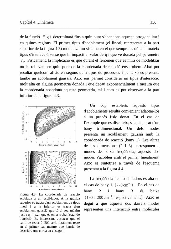
Capítol 4. Dinàmica 136__________________________________________________________________
de la funció F(q) determinarà fins a quin punt s'abandona aquesta ortogonalitat i
en quines regions. El primer tipus d'acoblament (el lineal, representat a la part superior de la figura 4.3) modelitza un sistema en el que sempre es dóna el mateix tipus d'interacció sense que hi impacti el valor de q i que ve donada pel paràmetre
c i . Físicament, la implicació és que durant el fenomen que es mira de modelitzar
no és rellevant en quin punt de la coordenada de reacció ens trobem. Això pot resultar quelcom afísic en segons quin tipus de processos i per això es presenta també un acoblament gaussià. Això ens permet considerar un tipus d'interacció molt alta en alguna geometria donada i que decau exponencialment a mesura que la coordenada abandona aquesta geometria, tal i com es pot observar a la part inferior de la figura 4.3.
Un cop establerts aquests tipus d'acoblaments resulta convenient adaptar-los a un procés físic donat. En el cas de l'exemple que es discuteix, s'ha disposat d'un bany tridimensional. Un dels modes presenta un acoblament gaussià amb la coordenada de reacció (bany 1). Les altres de les dimensions (2 i 3) corresponen a modes de baixa freqüència; aquests dos modes s'acoblen amb el primer linealment. Això es sintetitza a través de l'esquema presentat a la figura 4.4.
La freqüència dels oscil·ladors és alta en
el cas de bany 1 (770 cm−1) . En el cas de
bany 2 i bany 3 és baixa
(190 i 200 cm−1 , respectivament.) . Això és
degut a que aquests dos darrers modes representen una interacció entre molècules
Figura 4.3: La coordenada de reacció acoblada a un oscil·lador. A la gràfica superior es tracta d'un acoblament de tipus lineal i a la inferior es tracta d'un acoblament gaussià que té el seu màxim just a q=4 u.a., que és on es troba l'estat de transició. És interessant destacar que el camí de reacció IRC seria totalment recte en el primer cas mentre que hauria de descriure una corba en el segon.
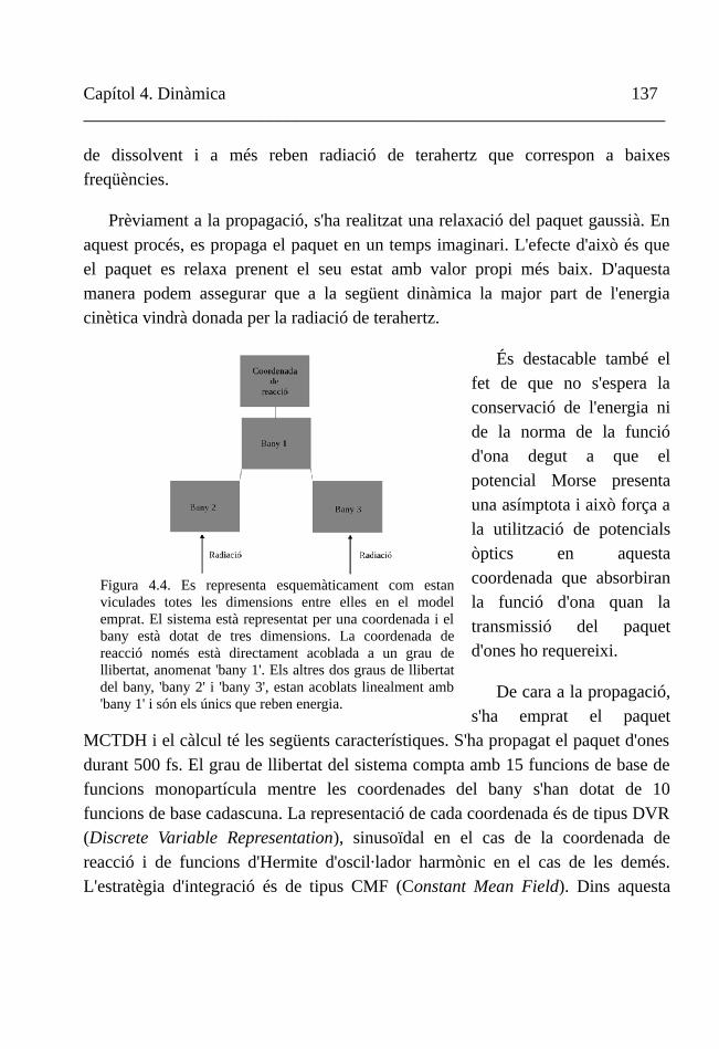
Capítol 4. Dinàmica 137__________________________________________________________________
de dissolvent i a més reben radiació de terahertz que correspon a baixes freqüències.
Prèviament a la propagació, s'ha realitzat una relaxació del paquet gaussià. En aquest procés, es propaga el paquet en un temps imaginari. L'efecte d'això és que el paquet es relaxa prenent el seu estat amb valor propi més baix. D'aquesta manera podem assegurar que a la següent dinàmica la major part de l'energia cinètica vindrà donada per la radiació de terahertz.
És destacable també el fet de que no s'espera la conservació de l'energia ni de la norma de la funció d'ona degut a que el potencial Morse presenta una asímptota i això força a la utilització de potencials òptics en aquesta coordenada que absorbiran la funció d'ona quan la transmissió del paquet d'ones ho requereixi.
De cara a la propagació, s'ha emprat el paquet
MCTDH i el càlcul té les següents característiques. S'ha propagat el paquet d'ones durant 500 fs. El grau de llibertat del sistema compta amb 15 funcions de base de funcions monopartícula mentre les coordenades del bany s'han dotat de 10 funcions de base cadascuna. La representació de cada coordenada és de tipus DVR (Discrete Variable Representation), sinusoïdal en el cas de la coordenada de reacció i de funcions d'Hermite d'oscil·lador harmònic en el cas de les demés. L'estratègia d'integració és de tipus CMF (Constant Mean Field). Dins aquesta
Figura 4.4. Es representa esquemàticament com estan viculades totes les dimensions entre elles en el model emprat. El sistema està representat per una coordenada i el bany està dotat de tres dimensions. La coordenada de reacció només està directament acoblada a un grau de llibertat, anomenat 'bany 1'. Els altres dos graus de llibertat del bany, 'bany 2' i 'bany 3', estan acoblats linealment amb 'bany 1' i són els únics que reben energia.
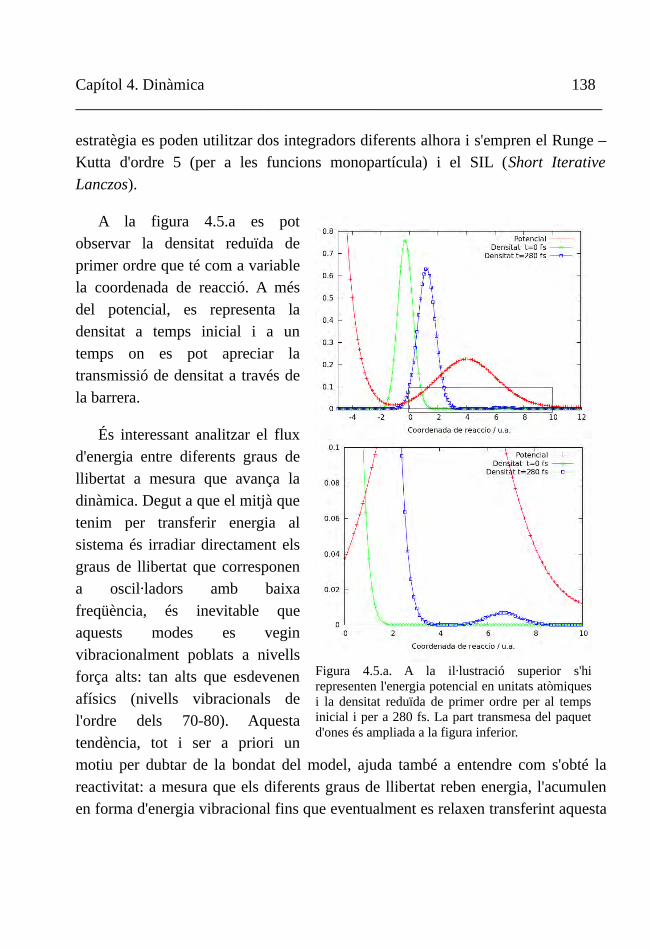
Capítol 4. Dinàmica 138__________________________________________________________________
estratègia es poden utilitzar dos integradors diferents alhora i s'empren el Runge – Kutta d'ordre 5 (per a les funcions monopartícula) i el SIL (Short Iterative Lanczos).
A la figura 4.5.a es pot observar la densitat reduïda de primer ordre que té com a variable la coordenada de reacció. A més del potencial, es representa la densitat a temps inicial i a un temps on es pot apreciar la transmissió de densitat a través de la barrera.
És interessant analitzar el flux d'energia entre diferents graus de llibertat a mesura que avança la dinàmica. Degut a que el mitjà que tenim per transferir energia al sistema és irradiar directament els graus de llibertat que corresponen a oscil·ladors amb baixa freqüència, és inevitable que aquests modes es vegin vibracionalment poblats a nivells força alts: tan alts que esdevenen afísics (nivells vibracionals de l'ordre dels 70-80). Aquesta tendència, tot i ser a priori un motiu per dubtar de la bondat del model, ajuda també a entendre com s'obté la reactivitat: a mesura que els diferents graus de llibertat reben energia, l'acumulen en forma d'energia vibracional fins que eventualment es relaxen transferint aquesta
Figura 4.5.a. A la il·lustració superior s'hi representen l'energia potencial en unitats atòmiques i la densitat reduïda de primer ordre per al temps inicial i per a 280 fs. La part transmesa del paquet d'ones és ampliada a la figura inferior.
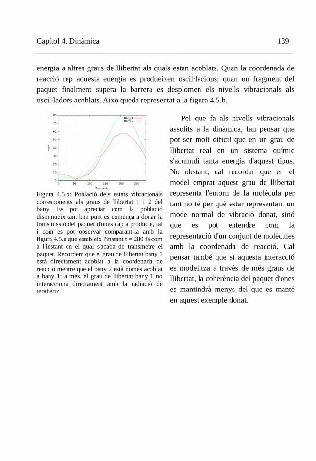
Capítol 4. Dinàmica 139__________________________________________________________________
energia a altres graus de llibertat als quals estan acoblats. Quan la coordenada de reacció rep aquesta energia es produeixen oscil·lacions; quan un fragment del paquet finalment supera la barrera es desplomen els nivells vibracionals als oscil·ladors acoblats. Això queda representat a la figura 4.5.b.
Pel que fa als nivells vibracionals assolits a la dinàmica, fan pensar que pot ser molt difícil que en un grau de llibertat real en un sistema químic s'acumuli tanta energia d'aquest tipus. No obstant, cal recordar que en el model emprat aquest grau de llibertat representa l'entorn de la molècula per tant no té per què estar representant un mode normal de vibració donat, sinó que es pot entendre com la representació d'un conjunt de molècules amb la coordenada de reacció. Cal pensar també que si aquesta interacció es modelitza a través de més graus de llibertat, la coherència del paquet d'ones es mantindrà menys del que es manté en aquest exemple donat.
Figura 4.5.b: Població dels estats vibracionals corresponents als graus de llibertat 1 i 2 del bany. Es pot apreciar com la població disminueix tant bon punt es comença a donar la transmissió del paquet d'ones cap a producte, tal i com es pot observar comparant-la amb la figura 4.5.a que estableix l'instant t = 280 fs com a l'instant en el qual s'acaba de transmetre el paquet. Recordem que el grau de llibertat bany 1 està directament acoblat a la coordenada de reacció mentre que el bany 2 està només acoblat a bany 1; a més, el grau de llibertat bany 1 no interacciona directament amb la radiació de terahertz.

Capítol 4. Dinàmica 140__________________________________________________________________
II. Hamiltonià del camí de reacció (RPH)
II.1. El hamiltonià clàssic
El cost computacional de qualsevol mètode dins la dinàmica quàntica és molt sovint massa alt. És un gran èxit que un mètode com el MCTDH hagi pogut afrontar càlculs de fins a 24 graus de llibertat, però això és un fet absolutament excepcional. Quan es vol realitzar un càlcul en el camp de la dinàmica quàntica sobre un sistema molecular i no es tracta d'un sistema especialment reduït, la realització d'aproximacions i modelitzacions és inevitable. Un exemple l'hem vist a l'apartat anterior, on s'ha realitzat una modelització que reduïa graus de llibertat a mers oscil·ladors harmònics. En aquest apartat, amb un paral·lelisme força gran com es veurà a continuació, s'optarà per l'aproximació.
El mètode per tal de definir un hamiltonià emprant un camí de reacció és conegut com a hamiltonià del camí de reacció (en anglès, RPH, Reaction Path Hamiltonian). Va se proposat per primera vegada per Miller i col·laboradors11. La seva proposta és definir un camí de reacció monodimensional i projectar-hi a cada instant el moment tenint en compte l'entorn quadràtic del camí de reacció. Dit d'una manera més general, el hamiltonià de camí de reacció descriu una dinàmica restringida on la translació està totalment projectada a la tangent del camí escollit i els restants 3N-7 graus de llibertat són modes vibracionals perpendiculars al camí de reacció. L'energia potencial té, doncs, una forma tal com:
V (s ,Q1,... ,Q3N−7)=V s(s)+12∑i=1
3 N−7
ω(s)i2 Qi
2 (4.18)
La forma de l'operador cinètic no és trivial de determinar i varia tenint en compte quin cas s'estudia, ja s'ha d'expressar en aquestes coordenades i el seu moment conjugat.
Una segona versió del hamiltonià del camí de reacció és la presentada per

Capítol 4. Dinàmica 141__________________________________________________________________
Bofill i col·laboradors12. Aquesta proposta va més enllà d'una projecció de les coordenades i els moments i aposta per redefinir la lagrangiana i el hamiltonià d'acord amb el camí de reacció tractat. De la integral de la lagrangiana amb forma més recurrent:
∫t 0
t
L(q ,dqd t )dt=∫
t 0
t12 (
dqd t )
T
(dqd t )−V (q)dt (4.19)
on t és el paràmetre que caracteritza la corba extremalitzada, es pot fàcilment passar a una lagrangiana que depengui de les variables dq /d s i d t /d s , on s és la longitud d'arc que caracteritzarà el camí de reacció:
∫t 0
t
L(q ,dqd s
,d td s )ds=∫
t 0
t12 (
dqd t )
T
(d qd t )(
d td s )
−1
−V (q)(d td s )dt (4.20)
D'aquesta lagrangiana poden deduir-se dues equacions d'Euler – Lagrange que no són independents. El hamiltonià que se'n dedueix té la següent estructura:
H (s , ps)=12
ps2
(dqd s )
T
(d qd s )
+V (q (s)) (4.21)
amb un moment ps definit com a:
ps=(d qd s )
T
(dqd s )(
d sd t ) (4.22)
Les equacions anteriors poden ser formulades per a cenyir-se a una coordenada de reacció donada, com el IRC. Degut a raons pràctiques, el desenvolupament subsegüent no empra directament la longitud d'arc s com a coordenada sinó una magnitud relacionada:

Capítol 4. Dinàmica 142__________________________________________________________________
u ( s)=exp [∫s0
sds'
√gT g ] (4.23)
Si s'escull el camí IRC per tal de caracteritzar el hamiltonià clàssic, aquest pren la forma:
H RP− IRC u,pu =12
pu2
g0u u
2 H 0−I g0
12
g0T uH 0 H 0
−1 uH 0 g0 +W 0 (4.24)
on W0 agrupa tots els termes que no tenen cap dependència amb u. Es pot apreciar com el terme cinètic depèn directament de u. Per aquest motiu, es diu que hi ha un terme de massa que varia amb la posició. No obstant, l'interès del mètode en el present text recau més aviat en la versió quàntica que es desenvolupa a continuació.
II.2. El hamiltonià quàntic (QRPH)
Per tal de desenvolupar el hamiltonià quàntic al voltant del IRC, s'adopta la condició subsidiària:
r (q , s )=q−q (s)=0 (4.25)
La definició de l'operador cinètic del hamiltonià quàntic requereix partir de la definició 4.22 i la definició de moment quàntic, p= -iħ∇q. També cal tenir en compte la derivada de la restricció 4.25:
∂ r(q , s)∂s
=−d q(s)
d s (4.26)
El projector per al moment sobre el camí de reacció IRC el podem escriure de

Capítol 4. Dinàmica 143__________________________________________________________________
la següent manera:
p=∂ r q,s /∂ s ∂r q,s /∂ s
T
∂ r q,s /∂ s T∂r q,s /∂ s
p (4.27)
i amb aquesta expressió és senzill avaluar el terme pTp:
pT p=[ pT (∂ r (q,s )/∂ s ) (∂r (q,s )/∂ s)T
(∂ r (q,s )/∂ s )T (∂ r (q,s )/∂ s ) ][ (∂ r ( q,s )/∂ s ) (∂r (q,s )/∂ s)T
(∂ r ( q,s )/∂ s )T (∂r (q,s )/∂ s)p ]=
=( 1
(∂ r (q,s )/∂ s )T (∂r (q,s )/∂ s) )1/4
{ (∂ r (q,s ) /∂ s )T p
[ (∂r (q,s )/∂ s)T (∂r (q,s ) /∂s ) ]1 /4 }
×{ (∂r (q,s )/∂ s)T p
[ (∂r (q,s )/∂s )T (∂ r ( q,s )/∂ s ) ]1/4 }( 1
(∂ r (q,s )/∂ s )T (∂r (q,s )/∂ s) )1/4
(4.28)
Substituint parcialment la igualtat (4.26) a l'expressió (4.28) obtenim:
pT p=(1
(∂r (q,s )/∂ s)T(∂r (q,s ) /∂ s ) )
1/4
( dq ( s)
ds )T
p (1
(∂r (q,s )/∂ s)T(∂r (q,s) /∂ s ) )
1/4
×(1
(∂r (q,s )/∂s )T(∂r (q,s) /∂ s ) )
1 /4
( dq ( s)ds )
T
p (1
(∂r (q,s )/∂s )T(∂r (q,s) /∂ s ) )
1 /4
(4.29)
Tenint en compte la definició de moment quàntic i l'equació 4.26, obtenim l'expressió final del nostre operador d'energia cinètica:
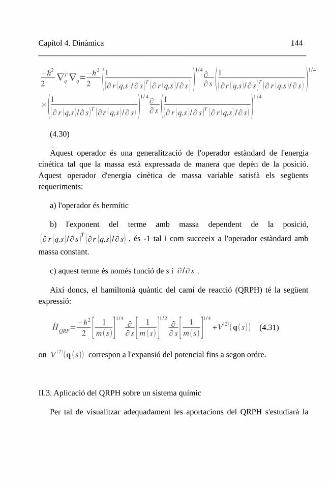
Capítol 4. Dinàmica 144__________________________________________________________________
−ℏ2
2∇q
T ∇q=−ℏ2
2 (1
(∂ r (q,s )/∂ s )T(∂ r (q,s )/∂ s ) )
1/4∂∂ s (
1
(∂r (q,s)/∂ s )T(∂ r (q,s )/∂ s ) )
1/4
×(1
(∂ r (q,s )/∂ s)T (∂r (q,s )/∂ s) )1/ 4
∂∂ s (
1
(∂ r (q,s )/∂ s )T (∂ r (q,s )/∂ s) )1 /4
(4.30)
Aquest operador és una generalització de l'operador estàndard de l'energia cinètica tal que la massa està expressada de manera que depèn de la posició. Aquest operador d'energia cinètica de massa variable satisfà els següents requeriments:
a) l'operador és hermític
b) l'exponent del terme amb massa dependent de la posició,
∂ r q,s /∂ s T∂r q,s /∂ s , és -1 tal i com succeeix a l'operador estàndard amb
massa constant.
c) aquest terme és només funció de s i ∂/∂ s .
Així doncs, el hamiltonià quàntic del camí de reacció (QRPH) té la següent expressió:
HQRP=−ℏ2
2 [ 1m(s) ]
1/4∂∂ s [
1m(s) ]
1/2∂∂ s [
1m(s) ]
1/4
+V (2 )(q(s)) (4.31)
on V (2)(q (s)) correspon a l'expansió del potencial fins a segon ordre.
II.3. Aplicació del QRPH sobre un sistema químic
Per tal de visualitzar adequadament les aportacions del QRPH s'estudiarà la

Capítol 4. Dinàmica 145__________________________________________________________________
seva aplicació sobre el sistema de clústers d'aigua i el radical hidroxil que s'ha estudiat utilitzant l'estructura electrònica al capítol 2.III.5.
Com que es tracta de sistemes on el moviment dels àtoms d'hidrogen pren molt de protagonisme, és esperable una contribució important de l'efecte túnel a qualsevol estudi dinàmic. Degut a aquest fet, l'us de dinàmica quàntica està justificat. Tenint en compte el nombre de graus de llibertat – són vuit àtoms i per tant divuit graus de llibertat en el cas de dues aigües i un radical – és imprescindible emprar alguna mena d'aproximació.
Al capítol 2, quan s'ha descrit la reacció d'una sola molècula d'aigua amb un radical hidroxil, s'ha mencionat una certa polèmica existent respecte al mecanisme de la reacció. Certament, hi ha certa controvèrsia pel que fa al paper del complex prereactiu. Aquest complex podria ser tant de tipus HOH...OH com el mínim
global H2 O...HO essent aquesta segona opció la que finalment s'ha emprat a
l'estudi presentat prèviament. El fet és que a l'estudi presentat13 es demostra l'existència d'un punt de transició entre vall i serralada. Aquest és un punt especial relacionat amb el punt d'inflexió – vall serralada presentat al capítol 3. Si un punt
d'inflexió vall – serralada es donava exclusivament quan com a mínim un valor propi de la matriu hessiana era nul i, a més, ortogonal al gradient, parlarem d'un punt de transició vall – serralada quan aquesta segona condició no es compleixi: la curvatura nul·la de la superfície ve donada per una combinació concreta de vectors propis de la hessiana. Un punt com aquest s'ha localitzat emprant una funció d'ona tipus CASSCF / 6-311 + G(2df,2p). Topològicament, aquest punt actua com una bifurcació que fa que les dues opcions
Figura 4.6: Representació de la funció de transmissió per a la reacció del radical hidroxil amb una molècula d'aigua. Es presenten dues transmissions diferents: una correspon a una dinàmica amb massa fixa i l'altra a una dinàmica amb QRPH.

Capítol 4. Dinàmica 146__________________________________________________________________
contraposades per la polèmica siguin accessibles.
La segona opció, però, s'ha estudiat amb especial atenció emprant el mètode QRPH. Es presenten dos perfils de reactivitat. En aquests perfils, es representa la probabilitat de transmissió en funció de l'energia. Aquesta mena de perfils s'obtenen efectuant una transformada de Fourier sobre les funcions d'autocorrelació de la propagació per tal de passar del domini temporal al domini energètic. Respecte als dos perfils presentats, es tracta del resultat QRPH etiquetat com a 'massa variable' i del resultat d'una propagació unidimensional emprant el perfil energètic IRC etiquetat com a 'massa constant'. Aquesta comparació és interessant per tal de fer notar quines aportacions realitza el mètode. A la figura 4.6 es pot valorar com es dóna un elevat efecte túnel que ve magnificat per l'efecte dels graus de llibertat ortogonals al camí de reacció tinguts en compte al QRPH. També és possible notar una major contribució a l'efecte antitúnel un cop superada la barrera clàssica, que ve senyalada amb una línia negra a aproximadament 12.5 kcal/mol. En comparació amb el cas de dues aigües (figura 4.7), es pot observar un efecte antitúnel molt major.
A la figura 4.7 es representen dues funcions de transmissió amb les seves corresponents anàlogues de massa constant. Corresponen ambdues a la reacció del radical hidroxil amb dues molècules d'aigua i tenen com a tret distintiu el fet de correspondre a IRCs que culminen en estats de transició diferent: el TS2 i el TS2a. Mostren comportaments pràcticament idèntics amb el lògic desplaçament energètic.
Si es fa la comparació entre els perfils per al cas d'una i dues aigües es pot fer una observació: l'efecte túnel és de magnitud
Figura 4.7. Es mostra la funció de transmissió per a la reacció del radical hidroxil amb dues molècules d'aigua. Es representa la corba corresponent a l'estat de transició TS2 i la corrresponents a l'estat de transició TS2a. En ambdós casos, s'inclou també la corba per a la propagació amb massa constant, és a dir, una propagació unidimensional amb un hamiltonià convencional.
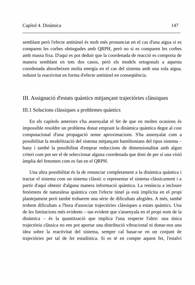
Capítol 4. Dinàmica 147__________________________________________________________________
semblant però l'efecte antitúnel és molt més pronunciat en el cas d'una aigua si es comparen les corbes obtingudes amb QRPH, però no si es comparen les corbes amb massa fixa. D'aquí es pot deduir que la coordenada de reacció es comporta de manera semblant en tots dos casos, però els models ortogonals a aquesta coordenada absorbeixen molta energia en el cas del sistema amb una sola aigua, reduint la reactivitat en forma d'efecte antitúnel en conseqüència.
III. Assignació d'estats quàntics mitjançant trajectòries clàssiques
III.1 Solucions clàssiques a problemes quàntics
En els capítols anteriors s'ha assenyalat el fet de que en moltes ocasions és impossible resoldre un problema donat emprant la dinàmica quàntica degut al cost computacional d'una propagació sense aproximacions. S'ha assenyalat com a possibilitat la modelització del sistema mitjançant hamiltonians del tipus sistema – bany i també la possibilitat d'emprar reduccions de dimensionalitat amb algun criteri com pot ser el de seleccionar alguna coordenada que doni de per sí una visió àmplia del fenomen com es fan en el QRPH.
Una altra possibilitat és la de renunciar completament a la dinàmica quàntica i tractar el sistema com un sistema clàssic o representar el sistema clàssicament i a partir d'aquí obtenir d'alguna manera informació quàntica. La renúncia a incloure fenòmens de naturalesa quàntica com l'efecte túnel ja està implícita en el propi plantejament però també trobarem una sèrie de dificultats afegides. A més, també trobem dificultats a l'hora d'associar trajectòries clàssiques a estats quàntics. Una de les limitacions més evidents – tan evident que s'assenyala en el propi nom de la dinàmica – és la quantització que implica l'una respecte l'altre: una única trajectòria clàssica no ens pot aportar una distribució vibracional ni donar-nos una idea sobre la reactivitat del sistema, sempre cal basar-se en un conjunt de trajectòries per tal de fer estadística. Si es té en compte aquest fet, l'estalvi
Capítol 4. Dinàmica 148__________________________________________________________________
computacional és relatiu ja que el nombre de trajectòries clàssiques necessàries (de l'ordre dels milions en moltes ocasions) pot resultar també prohibitiu.
Destaquem doncs dos trets de les trajectòries clàssiques: un és el cost alt que tot i la simplificació metodològica segueixen comportant i un segon és la necessitat de models per tal d'assimilar la trajectòria clàssica a la quàntica de manera que un conjunt de trajectòries clàssiques puguin oferir la mateixa informació que una propagació quàntica. De cara al primer tret esmentat, el mètode que es presentarà en aquesta secció pretén alleujar aquesta càrrega computacional reduint considerablement el nombre de trajectòries necessàries per tal de poder convergir numèricament una distribució de tipus vibracional. Per tal de comentar el segon aspecte és interessant primer esmentar el concepte de límit clàssic de la mecànica quàntica.
El límit clàssic de la mecànica quàntica
La física clàssica descriu molt satisfactòriament el comportament d'objectes macroscòpics. No obstant, falla quan es tracta de descriure sistemes microscòpics tal i com s'ha esmentat anteriorment. El límit clàssic de la mecànica quàntica sorgeix de la necessitat d'ubicar en algun punt una transició entre els sistemes que es poden tractar amb mecànica clàssica i els que s'han de tractar amb mecànica quàntica. L'existència d'aquest límit no ha estat mai provat amb rigor; es consideren diverses variables que poden fer canviar el comportament d'uns sistema de quàntic a clàssic: la massa, l'acció, un nombre quàntic... la condició més acceptada a la bibliografia és la de que la constant de Planck tendeixi a zero.2
Un pont recurrent entre la mecànica clàssica i la quàntica és la propagació de paquets gaussians a través de potencials parabòlics. Això és degut a que tant el valor esperat de la posició com el del moment es poden predir en aquests casos emprant mecànica clàssica. Això és fàcil d'entendre tenint en compte el clar paral·lelisme existent entre el teorema d'Ehrenfest i l'equació de Liouville.

Capítol 4. Dinàmica 149__________________________________________________________________
En aquest context, Heller descriu mitjançant equacions la propagació semiclàssica d'un paquet d'ones14. Si s'expandeix el potencial en una sèrie fins a
segon ordre al voltant d'un punt q0 s'obté el següent hamiltonià per a l'entorn
quadràtic:
H=− h
4 π2 m∇ q
2+V 0+g0
T(q−q0)+
12(q−q0)
T H 0(q−q0) (4.32)
on g0T i H0 són el vector gradient i la matriu hessiana al punt q0 (són
unidimensionals en aquest cas, és a dir, escalars). A continuació es pot establir un paquet gaussià referenciat respecte aquest puntc.
Ψ(q ,t )=exp(2π hγ0∣q−q0∣
2+
2π i h
p0T(q−q0)+
2πi h
α0) (4.33)
Els paràmetres γ0 i α0 són nombres complexos que determinen l'amplitud i la
normalització del paquet d'ones, respectivament. A més, γ0 ha de ser un nombre
negatiu en la seva part real i és interessant destacar que la normalització depèn de
α0 degut a que limq→∞
Ψ(q , t)=exp (2π iα0/ h ) . Degut a aquesta estructura, es pot
demostrar que q0 i p0 són exactament el valor esperat de la posició i el moment
per al paquet d'ones.
Si inserim les equacions 4.32 i 4.33 dins l'equació de Schrödinger i separem
per potències de (q−q0) obtenim tres equacions:
c El lector atent haurà notat que en altres capítols la funció d'ona es planteja amb una estructura diferent. Aquesta, que és l'emprada per Heller per tal de descriure la seva metodologia semiclàssica i la més habitual en la implementació computacional, no compta amb una amplada explícita igual que l'estructura R (q )ei /ℏ S(q) que s'ha emprat en altres capítols. La conciliació d'ambdues estructures ve donada pel fet de que R(q) i S(q) són nombres reals mentre que γ0 i α0 són complexos. És a la part real de γ0 i la imaginària de α0 on trobarem l'amplitud de la funció d'ona, com és evident si s'analitza el producte
Ψ *(q)Ψ(q)=exp (4 π /h(∣q−q0∣2Re (γ0)+Im(α0))) , tot i que el terme α0 només té valor de
cara a la normalització.

Capítol 4. Dinàmica 150__________________________________________________________________
∂γ0
∂ t=−
2m
γ02−
12
H 0
2γ0
∂q0
∂ t−∂ p0
∂ t=
2 γ0 p0
m+g0
∂α0
∂ t=
i h γ0
2πm+ p0
∂ q0
∂ t−V 0−
p02
2m
(4.34)
Aquestes equacions determinaran l'evolució temporal del paquet d'ones. Per tal de mostrar la connexió amb les equacions clàssiques hi ha prou amb introduir com
a hipòtesi l'equació de Hamilton ∂ q0/∂ t=p0 /m a la segona equació de les 4.34
per obtenir una altra equació de Hamilton: ∂ p0 /∂ t=−g .
En els mètodes quasiclàssics presents a la bibliografia és habitual realitzar previsions sobre el valor esperat d'observables quàntics mitjançant simplement una assignació de l'estat del sistema basant-se en la proximitat del valor obtingut al punt final d'una trajectòria clàssica. En el present text es proposa anar un pas més enllà i mirar de reconstruir la funció d'ona del model semiclàssic de Heller
aprofitant al màxim la informació final d'una trajectòria clàssica: q0 i p0 .
D'aquesta manera, amb una funció d'ona reconstruïda, serà possible calcular el valor esperat de tota mena d'observables emprant una projecció com si d'una dinàmica semiclàssica es tractés.
L'assignació d'estats quàntics és un tema amb un cert recorregut a la bibliografia. A continuació es comentaran alguns dels més emprats centrant la discussió en l'estimació de distribucions vibracionals. Aquests mètodes es denominen amb el terme anglosaxó binning.

Capítol 4. Dinàmica 151__________________________________________________________________
III.2 Els mètodes de binning
Mètode de trajectòries quasi-clàssiques
Aquest mètode, abreujat TQC i també anomenat binning histogràmic, és l'aproximació més immediata des del punt de vista intuïtiu. Consisteix a assignar el punt final de cada trajectòria clàssica a un estat quàntic assumint que l'estat que li correspondrà és el que tingui un valor propi més proper a l'energia vibracional en aquest punt. Així, la distribució vibracional es construeix a partir del recompte de trajectòries a cada nivell segons l'expressió següent. La població del nivell vibracional i - èssim serà:
PTQC(i)
=
∑j
n j(i)
∑i , j
n j(i)
(4.35)
on ∑j
n j( i) és el nombre de trajectòries que acaben amb l'estat vibracional i –
èssim com a estat més proper; i on destaca el fet que el sumatori al denominador és igual al número total de trajectòries i té com a únic propòsit el de normalitzar la distribució. Aquesta metodologia topa amb una sèrie de qüestions que en dificulten o limiten l'aplicabilitat: una major diferència d'energia entre nivells vibracionals fa que l'assignació d'estats es torni més arbitrària i això incideix en la bondat del mètode.
Binning gaussià
Una possible millora és la proposada per Bonnet i Rayez15,16. La seva aproximació, anomenada binning gaussià, consisteix en ponderar els pesos d'una manera més sofisticada que la del mètode de trajectòries quasi-clàssiques: emprant una funció gaussiana que decau exponencialment a mesura que l'estat més proper al punt final d'una trajectòria j – èssima s'allunya del nivell del qual la població s'està estimant:

Capítol 4. Dinàmica 152__________________________________________________________________
P BG(i)=
∑j
β√π exp (−β2
(n j−n(i))
2)
N traj
(4.36)
on N traj és el nombre total de trajectòries, n j és l'enter que correspon a l'estat
quàntic més proper a l'instant escollit per a la trajectòria j – èssima i n(i ) és el nombre quàntic de l'estat i – èssim per al qual estem analitzant la població. El
paràmetre β està relacionat amb l'amplada de la gaussiana descrita: com més
estreta sigui menys contribuirà a la població d'un determinat estat vibracional la trajectòria que acabi amb un nombre quàntic diferent; a la vegada, també seran necessàries més trajectòries per tal de convergir numèricament la distribució.
El fet de determinar el pes d'una trajectòria mitjançant la diferència entera entre nombres quàntics és totalment equivalent a fer-ho emprant diferències d'energies si considerem que l'oscil·lador harmònic és un model adient. D'aquesta manera, l'equació 4.36 passa a ser:
P 1BG(i)
=∑
j
β√π exp (−β2
((E j−E i)/2 E0)2 )
N traj
(4.37)
on E j és l'energia vibracional que correspon a la trajectòria analitzada i Ei
l'energia del nivell analitzat. E0 és la diferència d'energia entre dos nivells
contigus de l'oscil·lador o l'energia del punt zero. Si el càlcul és així la resta dins l'exponencial no està formada per enters com a la equació 4.36 sinó que degut al seu origen clàssic de les energies hi apareixerà l'equivalent a diferències de nombres quàntics que no seran enters. Aquesta segona aproximació es denomina 1BG i té la virtut de reduir el nombre de trajectòries necessàries per tal de convergir numèricament les distribucions.

Capítol 4. Dinàmica 153__________________________________________________________________
Altres aportacions
Les tècniques aquí exposades han experimentat, al llarg dels anys, alguns refinaments. Per exemple, Schatz17 i col·laboradors van establir que en processos reactius on un nombre elevat de trajectòries finalitzen per sota de l’energia vibracional del punt zero, s’obtenen resultats força correctes si simplement s’ignoren aquestes trajectòries.
El problema del binning histogràmic apareix també en el còmput d’altres magnituds, com la secció eficaç diferencial. Per tal de fer front a aquesta mena de distribució, Kosmas, Gislason i Jorgensen van proposar un mètode de filtrat gaussià que, en certs aspectes, té punts de coincidència amb la metodologia que es presentarà a continuació18.
Altres propostes, no tan lligades amb el binning final, però si amb el mostreig de condicions inicials, contemplen la generació aleatòria d’estats inicials, a partir de la distribució de Wigner19,20. Seguint aquesta línia metodològica, una altra proposta de Heller21,22 permet utilitzar trajectòries en un context mecanoquàntic fins el punt que l’estat final de les trajectòries s’utilitza per generar densitats de Wigner amb les que es calculen probabilitats de transició. El mètode de Heller–Wigner és un precedent força significatiu de la proposta que es detalla a continuació, tot i que aquest nou mètode introdueix més aproximacions.
III.3. El mètode de binning basat en la projecció de paquets d'ona clàssics
Descripció del mètode
Aquesta metodologia que anomenarem abreujadament BPPOC ens permetrà associar una sola trajectòria a diversos estats vibracionals alhora amb un evident estalvi computacional.

Capítol 4. Dinàmica 154__________________________________________________________________
En anteriors metodologies hem vist com s'emprava la proximitat de l'energia vibracional d'una trajectòria al valor propi de l'energia vibracional pròpia del sistema per tal de valorar la població de cada estat. Aquest nou mètode proposa partir d'una proposta similar a la de Heller per tal de calcular directament el recobriment del paquet d'ones semiclàssic amb les funcions pròpies del hamiltonià escollit per tal de representar les vibracions del sistema (oscil·lador harmònic, Morse...). En els estudis de Heller s'ha vist prèviament que es propaga un paquet gaussià emprant una sèrie d'equacions semiclàssiques calculant a cada punt una nova posició, moment, amplada i un factor de normalització.
En el cas del BPPOC el paquet semiclàssic no provindrà d'una propagació feta amb les equacions semiclàssiques sinó que es prendrà d'una trajectòria clàssica tant la posició final com el moment final i s'assignarà una amplada arbitrària; aquest procés es repetirà per a cada trajectòria clàssica d'un conjunt d'elles. El fet de que l'amplada sigui arbitrària cal pensar que tindrà algun efecte sobre la distribució vibracional; un dels objectius d'aquest treball és demostrar numèricament que l'efecte de la variació de l'amplada és petit.
El procediment operatiu associat al mètode és esquemàticament el següent:
a) Es calcula un conjunt de trajectòries clàssiques
b) Es decideix un criteri per tal d'aturar les trajectòries. Bàsicament, això pot ser un temps final o un hiperpla en l'espai de configuracions. Totes dues opcions tenen avantatges però a la implementació emprada per obtenir els següents resultats s'ha emprat el criteri temporal.
c) S'associa un paquet d'ones gaussià a la posició i moment finals de la trajectòria. L'estructura d'aquest paquet d'ones és la definida a l'equació 4.33.
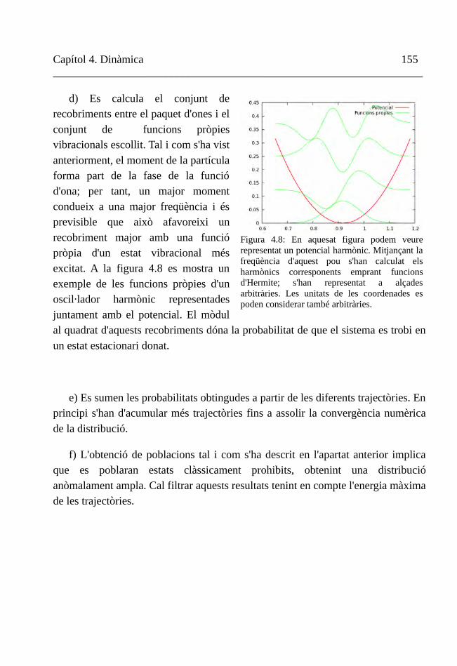
Capítol 4. Dinàmica 155__________________________________________________________________
d) Es calcula el conjunt de recobriments entre el paquet d'ones i el conjunt de funcions pròpies vibracionals escollit. Tal i com s'ha vist anteriorment, el moment de la partícula forma part de la fase de la funció d'ona; per tant, un major moment condueix a una major freqüència i és previsible que això afavoreixi un recobriment major amb una funció pròpia d'un estat vibracional més excitat. A la figura 4.8 es mostra un exemple de les funcions pròpies d'un oscil·lador harmònic representades juntament amb el potencial. El mòdul al quadrat d'aquests recobriments dóna la probabilitat de que el sistema es trobi en un estat estacionari donat.
e) Es sumen les probabilitats obtingudes a partir de les diferents trajectòries. En principi s'han d'acumular més trajectòries fins a assolir la convergència numèrica de la distribució.
f) L'obtenció de poblacions tal i com s'ha descrit en l'apartat anterior implica que es poblaran estats clàssicament prohibits, obtenint una distribució anòmalament ampla. Cal filtrar aquests resultats tenint en compte l'energia màxima de les trajectòries.
Figura 4.8: En aquesat figura podem veure representat un potencial harmònic. Mitjançant la freqüència d'aquest pou s'han calculat els harmònics corresponents emprant funcions d'Hermite; s'han representat a alçades arbitràries. Les unitats de les coordenades es poden considerar també arbitràries.

Capítol 4. Dinàmica 156__________________________________________________________________
Reaccions estudiades
S'han estudiat una sèrie de reaccions considerades en aproximació col·lineal. Ambdues són conegudes i freqüentades a la bibliografia i per tant sovint emprades per tal d'avaluar la bondat dels nous mètodes. Es poden representar com a un estat de transició que porta a dos estats asimptòtics; la superfície escollida per a modelitzar les reaccions és un pla bidimensional de la LEPS.
La reacció F+H2
La reacció és força exoèrgica, amb una diferència entre reactius i productes de 133 kcal/mol. Pràcticament no hi ha barrera, amb un estat de transició 4 kcal/mol per sobre de l'asímptota de reactius.
A continuació l'aplicació de del BPPOC exigeix el càlcul de les funcions vibracionals pròpies a l'asímptota de productes. En aquest cas, han estat obtingudes emprant una rutina numèrica de càlcul de valors i vectors propis a partir de la representació en DVR (representació de la variable discreta. De l'anglès, Discrete Variable Representation)
De cara al càlcul de trajectòries, s'ha escollit el criteri d'aturar-les a un temps donat. El major inconvenient associat a aquest criteri és el de que si acaben a una regió de l'espai de configuracions molt diferent, les freqüències associades poden ser diferents i per tant la construcció de la distribució vibracional inadequada. No obstant, el tipus de superfície emprada esquiva aquest inconvenient: el canal de productes manté la seva estructura quadràtica durant tota l'asímptota.
Les condicions inicials s'han escollit de manera que totes les trajectòries tenen una mateixa energia total, però les coordenades inicials s'han assignat seguint una distribució gaussiana al voltant d'un punt a l'espai de configuracions a l'asímptota de reactius. Aquest punt és el (3.9, 0.75).
Pel que fa al càlcul de recobriments, s'adjunta a mode d'exemplificació la taula

Capítol 4. Dinàmica 157__________________________________________________________________
en la qual es pot comparar per a una posició final i moment final donats com l'estat que s'assignaria emprant el binning histogràmic coincideix amb l'estat més poblat emprant el BPPOC. Addicionalment obtenim certa població als estats propers.
qf pf hbin v’=0 v’=1 v’=2 v’=3 v’=4 v’=5
0.83 13.30 1 0.77 1.00 0.56 0.24 0.14 0.09
0.97 16.30 1 0.49 1.00 0.70 0.19 0.01 0.01
0.87 16.40 1 0.54 1.0 0.72 0.29 0.10 0.05
1.02 7.13 0 1.00 0.67 0.16 0.07 0.01 0.00
Les poblacions obtingudes són correctes, tal i com es pot comprovar a la bibliografia tan teòrica com experimental23.
És rellevant esmentar que s'han realitzat proves amb diferents gammes. Els resultats presentats corresponen a una γ=30 u.a. que s'ha cregut oportuna per
tenir una amplada escaient en comparació a l'amplada del canal. Variacions raonables d'aquest paràmetre no provoquen una variació de la posició del màxim de la distribució ni de la seva amplada.
A les figures 9 i 10 trobem els resultats del mètode ja en forma de distribució. La figura 9 correspon a una distribució on s'han emprat 300 trajectòries. A la figura 10 trobem una representació per a dues energies més altes que en el cas anterior. Concretament són de 0.42 eV i 0.87 eV. S'han emprat 30 trajectòries.

Capítol 4. Dinàmica 158__________________________________________________________________
La reacció H 3C+H−CH 3→H3 C−H+CH3
Aquesta és una reacció de bescanvi d'hidrogen que representem també de forma col·lineal. Els dos graus de llibertat seran les distàncies C-H de l'hidrogen que es bescanvia. Durant el bescanvi, els altres hidrògens són un impediment estèric a qualsevol altra mena de mecanisme de manera que això fonamenta en part l'aproximació.
Respecte a la reacció estudiada a l'apartat anterior, la principal diferència és la freqüència dels canals asimptòtics que és més baixa en aquest cas.
L'estudi d'aquest sistema ens permet posar un exemple sobre la rapidesa de
Figura 4.10: S'exposen dues distribucions. S'han obtingut mitjançant 30 trajectòries. Es distingeixen per l'energia total de les trajectòries. La figura de l'esquerra correspon a 0.42eV i la de la dreta a 0.87 eV; no obstant, les distribucions són semblants degut al diferent repartiment de l'energia vibracional a l'instant escollit per tal de parar la dinàmica. L'amplada de la distribució prevista pel BPPOC torna a ser, de nou, lleugerament superior.
Figura 4.9: Distribució vibracional obtinguda mitjançant 300 trajectòries. La línia vermella mostra la distribució vibracional obtinguda amb binning histogràmic. Les línies blaves mostren la successiva convergència del mètode BPPOC i il·lustren la ràpida convergència del mateix. És destacable la semblança de la distribució excepte pel que fa a l'amplada, una mica superior, del BPPOC.
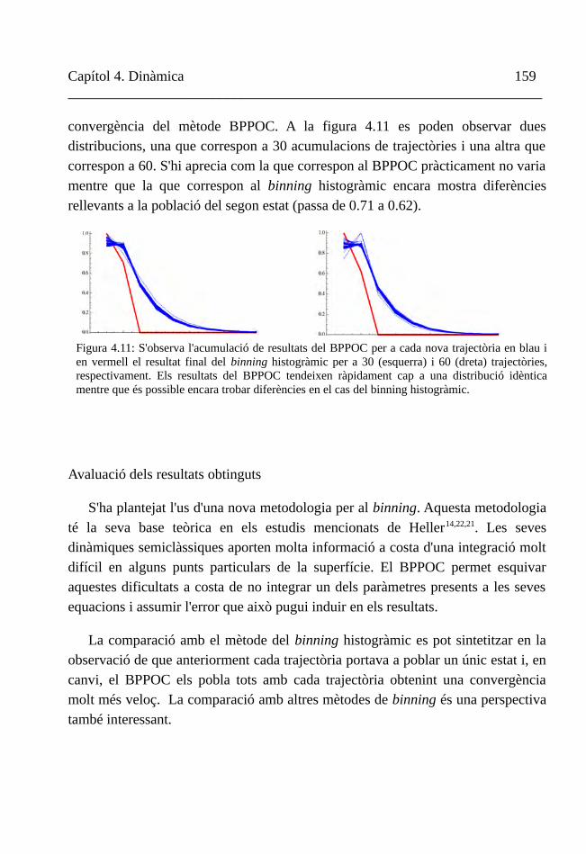
Capítol 4. Dinàmica 159__________________________________________________________________
convergència del mètode BPPOC. A la figura 4.11 es poden observar dues distribucions, una que correspon a 30 acumulacions de trajectòries i una altra que correspon a 60. S'hi aprecia com la que correspon al BPPOC pràcticament no varia mentre que la que correspon al binning histogràmic encara mostra diferències rellevants a la població del segon estat (passa de 0.71 a 0.62).
Avaluació dels resultats obtinguts
S'ha plantejat l'us d'una nova metodologia per al binning. Aquesta metodologia té la seva base teòrica en els estudis mencionats de Heller14,22,21. Les seves dinàmiques semiclàssiques aporten molta informació a costa d'una integració molt difícil en alguns punts particulars de la superfície. El BPPOC permet esquivar aquestes dificultats a costa de no integrar un dels paràmetres presents a les seves equacions i assumir l'error que això pugui induir en els resultats.
La comparació amb el mètode del binning histogràmic es pot sintetitzar en la observació de que anteriorment cada trajectòria portava a poblar un únic estat i, en canvi, el BPPOC els pobla tots amb cada trajectòria obtenint una convergència molt més veloç. La comparació amb altres mètodes de binning és una perspectiva també interessant.
Figura 4.11: S'observa l'acumulació de resultats del BPPOC per a cada nova trajectòria en blau i en vermell el resultat final del binning histogràmic per a 30 (esquerra) i 60 (dreta) trajectòries, respectivament. Els resultats del BPPOC tendeixen ràpidament cap a una distribució idèntica mentre que és possible encara trobar diferències en el cas del binning histogràmic.
Capítol 4. Dinàmica 160__________________________________________________________________
Els resultats preliminars obtinguts fan pensar que una amplada arbitrària del paquet d'ones no provoca alternacions substancials al càlcul de distribucions vibracionals. En canvi, l'estalvi computacional que es planteja a l'hora de convergir les distribucions queda confirmat. A banda d'això, és imprescindible emprar sistemes diferents per tal de trobar possibles punts febles del mètode.
També és convenient explorar com es comporta el mètode fora de la col·linealitat estricta.
IV. Conclusions
En els desenvolupaments que s'han dut a terme en aquest capítol hi ha un denominador comú: gairebé sempre és necessària una aproximació. Aquesta aproximació es duu a terme a nivell metodològic dins el camp de la dinàmica quàntica – ja sigui emprant un model per simplificar el problema o una aproximació sobre les equacions – o bé es porta al terreny de la mecànica clàssica canviant completament el paradigma o buscant un camp intermedi entre tots dos paradigmes com és la dinàmica semiclàssica.
En el camp de la modelització s'ha pogut constatar el gran esforç que és necessari per tal d'aproximar el model a la realitat. La bibliografia està plena de suggeriments però en totes elles sempre hi ha un punt d'arbitrarietat difícil d'enfocar. Això fa que un estudi dinàmic realitzat en aquestes condicions sigui de fet un estudi doble: un que tracta amb tota la complexitat de la dinàmica i un altre que tracta la manera de mantenir el model fisicomatemàtic en contacte amb la realitat.
Aquests dubtes s'esvaeixen si s'empren mètodes aproximats que eliminen graus de llibertat o utilitzen aproximacions d'alguna mena a la dinàmica quàntica. Efectivament, moltes vegades és possible tractar el problema sense haver de modelitzar el sistema. No obstant, la feina en aquesta ocasió recau en la pròpia

Capítol 4. Dinàmica 161__________________________________________________________________
justificació del mètode. El gran nombre de mètodes presents és testimoni suficient de que cap solució no és prou satisfactòria en tots els aspectes com per donar el problema per tancat.
L'aportació més innovadora realitzada en aquest capítol és el model d'activació tèrmica de reaccions emprant radiació de terahertz i el mètode BPPOC. Els resultats obtinguts i exposats més amunt fan pensar que ambdues línies són prometedores però cal encara aprofundir-hi per acabar de definir les virtuts i els defectes dels seus plantejaments, refinar-los i finalment dur-los a publicació.
Bibliografia
1. D. J. Tannor. Introduction to Quantum Mechanics. A time-dependent perspective. University Science Books (2007)
2. A. Messiah. Quantum Mechanics. North - Holland Publishing Company (1967)
3. A. Askar i A. S. Cakmak, The Journal of Chemical Physics, 68, 2794 (1978)
4. G. A. Worth, M. H. Beck, A. Jäckle i H. Meyer, The MCTDH Package, Version 8.2,(2000), University of Heidelberg, Heidelberg, Germany. H.-D. Meyer, Version 8.3 (2002),Version 8.4 (2007). See http://mctdh.uni-hd.de
5. S. Woutersen, U. Emmerichs i H. Bakker, Science, 278, 658 (1997)
6. H. Nguyen i W. Danen, Journal of the American Chemical Society, 103, 6253 (1981)
7. O. Kuhn i H. Naundorf, Phys. Chem. Chem. Phys., 5, 79 (2003)
8. R. Cukier i D. Nocera, Annual Review of Physical Chemistry, 49, 337 (1998)
9. J. Fang i S. Hammes-Schiffer, Journal of Chemical Physics, 106, 8442 (1997)
10. S. Cho i S. Shin, Journal of Molecular Structure - Theochem, 499, 1 (2000)
Capítol 4. Dinàmica 162__________________________________________________________________
11. W. H. Miller, N. C. Handy i J. E. Adams, The Journal of Chemical Physics, 72, 99 (1980)
12. J. Gonzalez, X. Gimenez i J. M. Bofill, Theoretical Chemistry Accounts, 112, 75 (2004)
13. J. Gonzalez, M. Caballero, A. Aguilar-Mogas, M. Torrent-Sucarrat, R. Crehuet, A. Solé, X. Giménez, S. Olivella, J. M. Bofill i J. M. Anglada, Theoretical Chemistry Accounts, 128, 579 (2011)
14. E. J. Heller, The Journal of Chemical Physics, 62, 1544 (1975)
15. L. Bonnet i J. Rayez, Chemical Physics Letters, 277, 183 (1997)
16. L. Bonnet i J. Espinosa-Garcia, The Journal of Chemical Physics, 133, 164108 (2010)
17. K. S. Bradley i G. C. Schatz, The Journal of Physical Chemistry, 98, 3788 (1994)
18. A. Kosmas, E. A. Gislason i A. D. Jorgensen, The Journal of Chemical Physics, 75, 2884 (1981)
19. H. Lee i M. O. Scully, The Journal of Chemical Physics, 73, 2238 (1980)
20. S. Goursaud, M. Sizun i F. Fiquet-Fayard, The Journal of Chemical Physics, 65, 5453 (1976)
21. R. C. Brown i E. J. Heller, The Journal of Chemical Physics, 75, 186 (1981)
22. E. J. Heller, The Journal of Chemical Physics, 65, 1289 (1976)
23. D. G. Truhlar, B. C. Garrett i N. C. Blais, The Journal of Chemical Physics, 80, 232 (1984)

Capítol 5
Conclusions
Capítol 5. Conclusions 164__________________________________________________________________
Les primeres línies escrites a la tesi parlen del desconcert d'un estudiant que enceta vida acadèmica – desconcert en bona part lligat als estudis de filosofia que també requerien atenció en aquell moment – i es troba tot de respostes diferents per a preguntes idèntiques, depenent de a quina disciplina se li faci la pregunta.
Durant els capítols dos, tres i quatre s'ha exposat el contingut de la recerca d'aquests anys de tesi doctoral. La incògnita plantejada s'ha mantingut durant tot aquest temps sense arribar a més conclusions al marge de les ja exposades al final del capítol primer: tota disciplina, per llunyana que sigui, es comunica amb les altres a través de paradigmes comuns; i si fins i tot això falla, ha de ser la vocació de servei a la societat el que les unifiqui. No hi pot haver mai una desconnexió total de la realitat, ni que sigui en els objectius últims d'una determinada recerca.
El més destacat en el sentit de l'aportació innovadora als diferents camps de la química teòrica per capítols són, a judici de l'autor, els següents:
- Del capítol d'estructura electrònica és destacable el fet de donar una eina matemàtica per tal d'analitzar en paral·lel la correlació electrònica de dues metodologies diferents: la funció d'ona i la teoria del funcional de la densitat. Aquest plantejament, que ens porta a ser crítics amb el DFT en alguns aspectes, també es pot veure com una manera de reflexionar sobre l'estructura matemàtica que ha de tenir el terme de correlació i bescanvi en un funcional.
- Del capítol de teoria de camins de reacció és destacable el fet de que es culmina l'elaboració de la base matemàtica en la qual es basen tres camins de reacció diferents: el IRC, les trajectòries newtonianes i els gradients extremals. A banda d'això, es planteja una nova manera de trobar interseccions còniques i es proposa un tipus de camí de reacció molt eficient a l'hora de trobar punts de sella, el GAD.
- Del capítol de dinàmica és destacable la col·laboració amb l'institut alemany CFEL (Center for Free Electron Laser) que dóna lloc a un model de tipus sistema – bany i proposa la iniciació de reaccions tèrmiques emprant radiació de terahertz. Per altra banda, la proposta del mètode de binning BPPOC és prometedora i

De la superfície d'energia potencial a la reactivitat química 165__________________________________________________________________
sembla que pot alleujar de manera important el cost computacional de l'estimació teòrica de certes distribucions.
En general, la tesi doctoral ha tocat amb la profunditat requerida en cada cas diversos aspectes fonamentals o aplicats de les tres disciplines mencionades més amunt, obtenint propostes interessants i també publicacions.
De la superfície d'energia potencial a la reactivitat química 166__________________________________________________________________
Agraïments
Si és qüestió d'agrair, el primer nom que em ve a la ment és Josep Maria Bofill. Si volen saber què ha fet aquest home per merèixer aquest privilegi dins els criteris ordinals d'aquesta secció els diré que ensenyar-me coses. Si volen saber què m'ha ensenyat, llegeixin la resta de pàgines d'aquest llibre. Tot i així, en confiança, els diré que de tot el que n'he après el meu coneixement preferit és el següent: ars longa, vita brevis. La relació que ens vincula la burocràcia l'ha batejat de moltes maneres tan redundants com prescindibles. Ell és el meu: tutor, director de tesi, investigador principal del grup... però si algú em preguntés per qui és ell per a mi, jo utilitzaria la paraula mentor.
Si seguim per la via dels 'agraïments acadèmics' també és de justícia agrair a totes les persones que han dedicat energies a fer-me millor químic en algun moment de la meva tesi i sense ser pas professors del màster. Ja sigui amb explicacions o recomanacions d'aquest tipus. A priori, tres noms venen a la meva ment. El meu codirector, en Xavi Giménez; la persona que es va cuidar de mi durant la meva estança a Hamburg, n'Oriol Vendrell; i un col·laborador molt habitual del grup que m'ha ensenyat molta estructura electrònica, l'Iberio de P. R. Moreira. També vull dedicar una línia a agrair a tota la gent del departament que siguin tan macos i maques.
Entrant més en el terreny personal i abandonant l'ambient purament acadèmic, un moment de record pels meus compis de despatx és inevitable.
Carlos, sempre et recordaré quan escolti la nostra cançó <3, what's going on...
I clar, la meva companya durant gairebé tota la tesi es mereix més que un parell de línies una oda simfònica complerta. Gràcies per papallonejar pel despatx quan em veus desanimat i alegrar-me els dies, Estefi.
Abandonant els pisos superiors i baixant al bar, és molt important tenir un moment de reconeixement per tota la feina duta a terme per la meva llotja Illuminati, els Puro Pelícano. Llarga vida i cosas.
De la superfície d'energia potencial a la reactivitat química 167__________________________________________________________________
Més lluny de la facultat hi tinc la família, els amics... gràcies a tots. No és que tingui massa a veure amb la tesi però quedava lleig no posar-ho.
Més lluny, a Madrid, hi ha els senyors que m'han pagat tots quatre anys. Ens hem portat molt bé durant tot aquest temps, excepte aquella vegada que no hi va haver paga extra. Aquell dia ens vam portar fatal. En fi, ningú és perfecte. La meva beca és la BES-2009-019316. Sóc sincer, gràcies. Tot i així, no s'ho prenguin malament si vaig fent via.
Molt, molt més lluny, a Doha, Qatar, hi tinc el focus de com a mínim la meitat dels meus pensaments diaris. Quines ganes de que tornis, princesita. Tant de bo em poguessis veure defensant aquesta tesi.

Apèndix
i
articles

Apèndix __________________________________________________________________
Apèndix A
L'equació característica de l'equació de derivades parcials hiperbòlica
Partim de la següent equació hiperbòlica de derivades parcials:
∇q2 ψ(q , ν)−G(q ) ∂
2
∂2 ν
ψ(q , ν)=0 (3.7) (A.1)
La funció ψ depèn de N coordenades, posem cartesianes, i una coordenada
addicional que és l'energia, ν . Transformarem aquest sistema de coordenades de manera que puguem resoldre l'equació mitjançant el mètode de característiques. Les noves coordenades seran el conjunt {x}. Aquestes coordenades estan definides per les següents N+1 funcions:
ϕi(q , ν)=x i=constant i=1,..., N+1 (A.2)
en contrast amb el conjunt {q} definit per a N variables; en complementarietat amb la variable addicional ν .
Amb aquestes definicions duem a terme la transformació. En primer lloc,
Φ(x )=Φ(ϕ1(q , ν) ,... ,ϕN+1(q , ν))=ψ(q ,ν) (A.3)
Si desenvolupem el primer terme prenent el producte escalar de l'operador de derivada parcial per si mateix:
∇q2 ψ(q , ν)=∑
i=1
N∂
2 ψ(q ,ν)
∂ qi2 (A.4)
i si aleshores apliquem la regla de la cadena obtindrem:
∂2 ψ(q ,ν)
∂q i2 =∑
j=1
N+1
{∂2 ϕ j
∂ qi2
∂Φ(x)
∂ x j
+∂ϕ j
∂ qi∑k=1
N+1 ∂ϕ k
∂q i
∂2 Φ(x)
∂ x j ∂ xk } (A.5)

De la superfície d'energia potencial a la reactivitat química __________________________________________________________________
De manera similar, per al segon terme de l'equació A.1, tenim:
∂2 ψ(q ,ν)
∂ ν2=∑
j=1
N+1
{∂2 ϕ j
∂ν2
∂Φ(x)
∂ x j
+∂ϕ j
∂ν ∑k=1
N+1 ∂ϕ k
∂ ν∂
2 Φ(x)
∂ x j∂ xk} (A.6)
Substituint a l'equació A.1 i reordenant termes i sumatoris:
∑j=1
N+1∂Φ(x)
∂ x j {∑i=1
N+1 ∂2ϕ j
∂ qi2 −G(q)
∂2 ϕ j
∂ ν2 }+
+∑j=1
N+1
∑k=1
N+1∂
2Φ(x)
∂ x j∂ xk{∑
i=1
N+1 ∂ϕ j
∂ qi
∂ϕ k
∂q i
−G(q)∂ ϕ j
∂ν
∂ϕk
∂ν }=0
(A.7)
Prendrà una notorietat diferenciada la variable xN +1 degut als valors inicials o
dades de Cauchy donats a la superfície definida per ella, ϕN+1(q , ν)=xN+1 :
Φ(x )∣xN +1=ν0i
∂Φ(x)
∂ xN+1∣xN +1=ν0
(A.8)
On ν0 és un valor de ν donat, una constant. També vindran donats:
∂Φ(x )
∂ x i∣xN +1=ν 0
i=1,... , N
∂2 Φ(x )
∂ xi ∂ xN+ 1∣xN +1=ν0
=∂
2Φ(x)
∂ xN+1 ∂ x i∣xN+1=ν0
i=1,..., N (A.9)
∂2 Φ(x)
∂ xi∂ x j∣xN+1=ν0
=∂
2 Φ(x )
∂ x j ∂ x i∣xN+1=ν 0
i , j=1,..., N
Totes aquestes derivades especificades com a dades conegudes estan definides
a la superfície ϕN+1(q , ν)=x N+1 . El pla tangent a cada punt d'aquesta superfície
és el pla característic. El vector normal a aquest pla indica la direcció de l'evolució
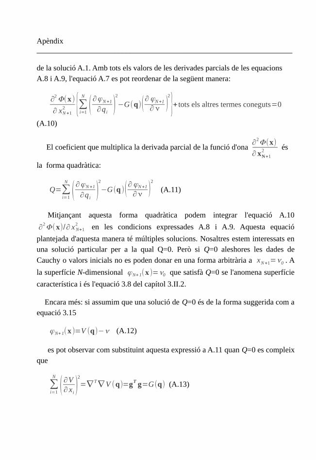
Apèndix __________________________________________________________________
de la solució A.1. Amb tots els valors de les derivades parcials de les equacions A.8 i A.9, l'equació A.7 es pot reordenar de la següent manera:
∂2 Φ(x )
∂ xN +12 {∑i=1
N
(∂ϕN+1
∂q i)
2
−G(q)(∂ϕN+1
∂ ν )2
}+ tots els altres termes coneguts=0
(A.10)
El coeficient que multiplica la derivada parcial de la funció d'ona ∂
2Φ(x)
∂ xN+12 és
la forma quadràtica:
Q=∑i=1
N
(∂ϕN +1
∂q i)
2
−G(q )(∂ϕN+1
∂ ν )2
(A.11)
Mitjançant aquesta forma quadràtica podem integrar l'equació A.10
∂2Φ(x)/∂ xN+1
2 en les condicions expressades A.8 i A.9. Aquesta equació
plantejada d'aquesta manera té múltiples solucions. Nosaltres estem interessats en una solució particular per a la qual Q=0. Però si Q=0 aleshores les dades de
Cauchy o valors inicials no es poden donar en una forma arbitrària a xN+1=ν0 . A
la superfície N-dimensional ϕN+1(x )=ν0 que satisfà Q=0 se l'anomena superfície
característica i és l'equació 3.8 del capítol 3.II.2.
Encara més: si assumim que una solució de Q=0 és de la forma suggerida com a equació 3.15
ϕN+ 1(x )=V (q)−ν (A.12)
es pot observar com substituint aquesta expressió a A.11 quan Q=0 es compleix que
∑i=1
N
(∂V∂ x i
)2
=∇ T ∇V (q)=gT g=G(q) (A.13)

De la superfície d'energia potencial a la reactivitat química __________________________________________________________________
que és l'equació eikonal de partida 3.5 presentada al capítol 3.II.2 que més endavant es pot resoldre reduitn-la a una família coneguda d'equacions diferencials ordinàries.

De la superfície d'energia potencial a la reactivitat química __________________________________________________________________
Apèndix B
De la mecànica clàssica a la mecànica quàntica amb principis variacionals1
En el principi de Fermat – Huygens s'exposa que la llum viatja entre dos punts seguint sempre el camí més curt possible i per tant això implica trobar una variació
de la fase de la funció d'ona (ϕ a una funció d'ona tal com Z=aexp (iϕ)) tal que
sigui mínima. Seguint els procediments propis de la mecànica quàntica, es planteja l'estacionarització no de la fase de l'ona sinó de l'acció; per això es proposa una funció d'ona en la que l'acció prengui un paper anàleg al de la fase:
ψ=aexp (iS /ℏ) (B.1)
L'acció, en mecànica clàssica, obeeix l'equació de Hamilton – Jacobi:
∂S∂ t
+1
2m ( ∂ S∂ x )
2
+U=0 (B.2)
En aquesta equació, el primer terme ∂ S /∂ t=−E . El segon terme és l'energia cinètica clàssica ja que ∂ S /∂ x=p ; derivant l'equació B.1 respecte la coordenada x podem obtenir la següent expressió per al momenta:
∂S∂ x
=−i ℏψ
∂ψ
∂ x (B.3)
i tenint en compte la naturalesa complexa de la funció d'ona podem reescriure l'equació de Hamilton – Jacobi de la següent forma:
−E+1
2m (∂ S∂ x )
*
(∂ S∂ x )+U=0 (B.4)
on l'asterisc marca la conjugada complexa. Per tant, obtenim:
a També s'ha d'incloure el supòsit addicional de que la derivada de l'amplitud ∂ a/∂ x tendeix a zero, o l'estructura del moment seria més complicada.
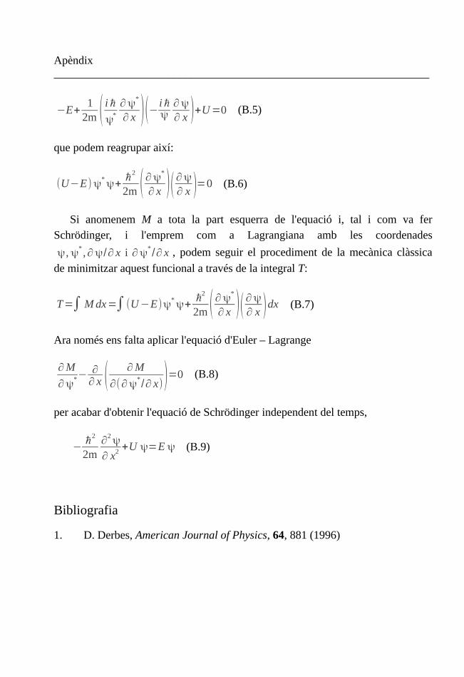
Apèndix __________________________________________________________________
−E+1
2m ( i ℏ
ψ*
∂ψ*
∂ x )(− i ℏψ
∂ψ
∂ x )+U=0 (B.5)
que podem reagrupar així:
(U−E) ψ*ψ+
ℏ2
2m (∂ψ*
∂ x )(∂ψ
∂ x )=0 (B.6)
Si anomenem M a tota la part esquerra de l'equació i, tal i com va fer Schrödinger, i l'emprem com a Lagrangiana amb les coordenades
ψ, ψ*,∂ψ/∂ x i ∂ψ*/∂ x , podem seguir el procediment de la mecànica clàssica
de minimitzar aquest funcional a través de la integral T:
T=∫ M dx=∫(U−E)ψ*ψ+
ℏ2
2m (∂ψ*
∂ x )(∂ψ
∂ x )dx (B.7)
Ara només ens falta aplicar l'equació d'Euler – Lagrange
∂M
∂ψ*−
∂∂ x ( ∂ M
∂(∂ψ*/∂ x))=0 (B.8)
per acabar d'obtenir l'equació de Schrödinger independent del temps,
−ℏ
2
2m∂
2ψ
∂ x2 +U ψ=E ψ (B.9)
Bibliografia
1. D. Derbes, American Journal of Physics, 64, 881 (1996)

De la superfície d'energia potencial a la reactivitat química __________________________________________________________________
Apèndix C
Tipus de funcionals de la densitat
Tal i com es menciona al capítol 2 al seu apartat dedicat a la teoria del funcional de la densitat (DFT), l'apartat III, de cara a establir les equacions de treball per a aquest mètode és molt rellevant de quina manera s'expressa el potencial de correlació – bescanvi.
Hi ha moltes aproximacions a la literatura. És poden classificar en diferents tipus segons quina dependència té el funcional. A partir de cada aproximació existeixen a més diferents parametritzacions, de manera que una infinitat de funcionals diferents han estat dissenyats. Gràficament, es pot expressar com a la figura C.11.
A continuació es planteja la divisió més comú entre funcionals. Es resumiran les característiques més definitòries de tots ells.2,3
Generalment l'energia a la que hom es refereeix és ϵXC , l'energia de correlació
bescanvi per partícula d'un gas uniforme de densitat ρ , que es defineix com a
EXC=∫ρ(x )ϵxc d x (C.1).
S'accepta que es pot dividir la contribució d'aquesta energia en una part de correlació i una de bescanvi:
ϵXC=ϵX+ϵC (C.2)
Figura C.1. Es mostra la rellevància de cada funcional segons el seu us a la bibliografia relacionant-la amb la grandària de les lletres. La imatge és obra de Peter Elliott.

Apèndix __________________________________________________________________
C.1 Aproximació de la densitat local (LDA)
La dependència és exclusivament de la densitat. Generalment, es tracten de forma separada la correlació i el bescanvi. És l'aproximació més senzilla. Pel que fa a la part de correlació, s'empra una expressió derivada per Bloch i Dirac als anys
20 que estableix una dependència directa de la densitat de l'ordre de ρ4 /3 :
ϵX=−34 (3ρ
π )1/3
(C.3)
Generalment aquest funcional és anomenat funcional de Slater.
No es coneix una expressió exacta per a la part de correlació. Tot i això, se'n modelitzen de basats en simulacions de tipus Monte Carlo sobre gas homogeni d'electrons4. S'han presentat funcionals dintre dels quals els més utilitzats són els basats en els estudis de Vosko, Wilk i Nusair; són els funcionals anomenats SVWN5. La variant més recomanada pels autors és la SVWN5 que és la que fa servir parametritzacions basades en els càlculs Monte Carlo esmentats.
Es considera que aquests funcionals donen bon resultats en quant a geometries – tot i que les distàncies d'enllaç tendeixen a aparèixer escurçades – bons espectres vibracionals i densitats de càrrega raonables excepte a les regions properes als nuclis. L'aproximació no és bona quan apareixen enllaços dèbils o en les prediccions termoquímiques. L'energia d'enllaç es sol exagerar aproximadament un 30%.
C.2 Aproximació del gradient generalitzat (GGA)
Com el seu nom indica, aquesta mena de funcional inclou el gradient de la densitat com a variable. Si ens referíem al LDA com a 'local', aquest funcional serà doncs 'semilocal' ja que té en compte l'entorn de cada punt.
EXC=∫ f (ρ , ∇ρ)d x (C.4)

De la superfície d'energia potencial a la reactivitat química __________________________________________________________________
Sense entrar en detall, aquesta mena de funcionals consisteixen en el desenvolupament de la densitat a un ordre superior (el gradient) de manera que el comportament asimptòtic i els forats definits siguin correctes. Això implica que la forma matemàtica d'aquests funcionals no ve donada per cap sentit físic sinó per pur pragmatisme: alguns d'aquests funcionals no estan basats en cap model físic.
Alguns dels funcionals més emprats són: PW916, BLYP7,8 i PBE9 .
Respecte a l'aproximació LDA tant les geometries com les freqüències milloren. Responen raonablement bé davant d'enllaços tipus ponts d'hidoregen però no són capaços de descriure correctament les interaccions tipus Van der Waals.
C.3 Aproximació meta – GGA
En el camp de l'aproximació meta – GGA es va una mica més lluny i s'incorporen més variables a l'energia de correlació – bescanvi: es tracta de la densitat de l'energia cinètica ( i de retruc l'ocupació orbital)
τ (x )=12∑i=1
N
∣∇ χi(x)∣2
(C.5)
i també la laplaciana de la densitat (la segona derivada) ∇2ρ(x)
EXC=∫ f (ρ, ∇ρ , τ ,∇ 2ρ)d x (C.6)
Val la pena destacar que el càlcul de la laplaciana de la densitat comporta una exigència computacional d'una reixeta (grid) amb més punts. Alguns funcionals meta – GGA destacables són revTPSS10, PKZB11 i VSXC12.
C.4 Mètodes híbrids
Els mètodes híbrids empren bescanvi extret directament d'un càlcul Hartree- Fock i l'incorporen al bescanvi que s'empra en el funcional en alguna proporció

Apèndix __________________________________________________________________
que varia en cada cas. El rerefons teòric que justifica aquesta pràctica s'anomena connexió adiabàtica. Hom distingeix els mètodes híbrids en híbrids GGA i híbrids meta – GGA depenent en si el bescanvi que empren prové d'un tipus de funcional o de l'altre.
Hi ha molts funcionals híbrids destacables. Sense cap mena de dubte el més emprat és el B3LYP13 com es pot veure a la figura 1. També en destacarem el PBE014, el BH&HLYP15 i el M0616.
Bibliografia
1. K. Burke, The Journal of Chemical Physics, 136, 150901 (2012)
2. W. Koch i M. C. Holthausen. A Chemist's Guide to Density Functional Theory. Wiley-VCH (2000)
3. M. Solà i J. M. Ugalde. Quantum Chemstry Methods: II Density Functional Theory. A Theoretical and Computational Chemistry: Foundations, Methods and Techniques. J. Andrés i J. Bertran (Eds.), (2007) 221-277.
4. D. Ceperley i B. Alder, Physical Review Letters, 45, 566 (1980)
5. S. Vosko, L. Wilk i M. Nusair, Canadian Journal of Physics, 58, 1200 (1980)
6. J. P. Perdew, J. A. Chevary, S. H. Vosko, K. A. Jackson, M. R. Pederson, D. J. Singh i C. Fiolhais, Phys. Rev. B, 46, 6671 (1992)
7. A. D. Becke, Phys. Rev. A, 38, 3098 (1988)
8. C. Lee, W. Yang i R. G. Parr, Phys. Rev. B, 37, 785 (1988)
9. J. P. Perdew, K. Burke i M. Ernzerhof, Physical Review Letters, 77, 3865 (1996)
10. J. Tao, J. P. Perdew, V. N. Staroverov i G. E. Scuseria, Physical Review Letters, 91, 146401 (2003)
11. J. P. Perdew, S. Kurth, A. Zupan i P. Blaha, Physical Review Letters, 82, 2544 (1999)
De la superfície d'energia potencial a la reactivitat química __________________________________________________________________
12. T. V. Voorhis i G. E. Scuseria, The Journal of Chemical Physics, 109, 400 (1998)
13. A. D. Becke, The Journal of Chemical Physics, 98, 5648 (1993)
14. C. Adamo i V. Barone, The Journal of Chemical Physics, 110, 6158 (1999)
15. A. D. Becke, The Journal of Chemical Physics, 98, 1372 (1993)
16. Y. Zhao i D. G. Truhlar, The Journal of Chemical Physics, 125, 194101 (2006)
THE JOURNAL OF CHEMICAL PHYSICS 138, 174107 (2013)
A comparison model between density functional and wave functiontheories by means of the Löwdin partitioning technique
Marc Caballero,1,2 Ibério de P. R. Moreira,1,2 and Josep Maria Bofill1,31Institut de Química Teòrica i Computacional, Universitat de Barcelona, IQTCUB, C/ Martí i Franquès 1,E-08028 Barcelona, Spain2Departament de Química Física, Universitat de Barcelona, C/ Martí i Franquès 1, E-08028 Barcelona, Spain3Departament de Química Orgànica, Universitat de Barcelona, C/ Martí i Franquès 1,E-08028 Barcelona, Spain
(Received 28 January 2013; accepted 1 April 2013; published online 2 May 2013)
A comparison model is proposed based on the Löwdin partitioning technique to analyze thedifferences in the treatment of electron correlation by the wave function and density functionalmodels. This comparison model provides a tool to understand the inherent structure of both theoriesand its discrepancies in terms of the subjacent mathematical structure and the necessary conditionsfor variationality required for the energy functional. Some numerical results on simple moleculesare also reported revealing the known phenomenon of “overcorrelation” of density functional theorymethods. © 2013 AIP Publishing LLC. [http://dx.doi.org/10.1063/1.4802200]
INTRODUCTION
The fundamental mathematical formulation of the non-relativistic many electron problem for a system defined byn electrons and N nuclei in interaction is the time indepen-dent Schrödinger equation. The corresponding exact solutionsprovide the essential quantum-mechanical description of eachelectronic state in terms of the different n electron wave func-tions �(r1s1, . . . , rnsn). The time independent Schrödingerequation for a system defined by n electrons and N nuclei ininteraction can be written as a Rayleigh-Ritz quotient givenby
E [�] =��| H |��
�� | ��(1)
in which the Hamiltonian operator is defined as
H = T + V + W (2)
with
T (r1, . . . , rn) = −1
2
n�
i=1
∇2(i),
V (r1, · · · , rn;R1; · · · ;RN )
=
n�
i=1
N�
I=1
−ZI
|RI − ri |=
n�
i=1
v(ri ;R1; · · · ;RN ),
W (r1, . . . , rn) =
n−1�
i=1
n�
j=i+1
1�
�ri − rj
�
�
=
n�
i>j=1
1
rij.
In this expression, the first term stands for the kinetic energyof the electrons, the second arises from the external poten-tial v(ri; R1; . . . ; RN) generated by the nuclei and 1/rij isthe two electron interaction. This Hamiltonian operator de-fines, along with its boundary conditions, an elliptic secondorder differential equation and the wave functions must sat-isfy some specific conditions to be an acceptable variationalsolution of Eq. (1). Since the non-relativistic many-electronHamiltonian does not act on spin coordinates, anti-symmetry
and spin restrictions must be imposed ad hoc in the wavefunction,�(r1s1, . . . , rnsn), so as to satisfy the Pauli principleand spin symmetry requirements of the quantum mechanicalstate of the system.
Defining γ 1 and γ 2, the usual one- and two-electron den-sity matrices directly obtained from the n-electron wave func-tion �(r1s1, . . . , rnsn), as
γ1(r1; r1�) = n
�
rn
· · ·
�
r2
�
sn
· · ·
�
s1
�(r1s1, · · · , rnsn)
×�∗(r1�s1, · · · , rnsn)ds1 · · · dsndr2 · · · drn, (3)
γ2(r1, r2; r1�, r2
�) =n(n − 1)
2
×
�
rn
· · ·
�
r3
�
sn
· · ·
�
s1
�(r1s1, r2s2, · · · , rnsn)
×�∗(r1�s1, r2
�s2, · · · , rnsn)ds1 · · · dsndr3 · · · drn, (4)
the most compact expression for the energy of the n-electronsystem in the field of N fixed nuclei can be written as
E[γ1, γ2] = −1
2
�
r1=r1�
[∇ · ∇T γ1(r1; r1�)]dr1
+
�
r1
v(r1;R1; . . . ;RN )γ1(r1)dr1
+
�
r2
�
r1
γ2(r1, r2)
r12dr1dr2 (5)
in which the many-electron quantities γ 1(r1) and γ 2(r1, r2)are the diagonal elements, γ 1(r1) = γ 1(r1; r1) and γ 2(r1, r2)= γ 2(r1, r2; r1, r2), of the spinless one- and two-electron den-sity matrices (Eqs. (3) and (4)), respectively.1–3 Notice thatthe former is the one-electron density ρ(r) commonly used
0021-9606/2013/138(17)/174107/5/$30.00 © 2013 AIP Publishing LLC138, 174107-1
Downloaded 08 Sep 2013 to 161.116.100.92. This article is copyrighted as indicated in the abstract. Reuse of AIP content is subject to the terms at: http://jcp.aip.org/about/rights_and_permissions

174107-2 Caballero, Moreira, and Bofill J. Chem. Phys. 138, 174107 (2013)
in electronic structure theory. Therefore, an accurate predic-tion of the energy of a given system in a given electronic staterequires a reasonable estimate of �(r1s1, . . . , rnsn). It is cus-tomary to expand �(r1s1, . . . , rnsn) in a known basis set andto find the expansion coefficients using the variational methodand with all necessary and sufficient constraints (spin and
space symmetries) to prevent the variational collapse.4 This isthe basis of the so-called Full Configuration Interaction (FCI)method which provides the exact variational solution for theenergy functional of the electronic system defined in Eq. (5)in a given basis set.
Equation (5) is the starting point of Density FunctionalTheory (DFT) which aims to replace both γ 1(r1; r1
�) andγ 2(r1, r2) by the one-electron density, γ 1(r1). For the groundstate, this wish is justified by the celebrated Hohenberg-Kohn(HK) theorems, which state that the exact ground state totalenergy of any many-electron system is given by a universal,unknown, functional of the electron density only.5 Rigorouslyspeaking, only the second term of the right hand side part ofEq. (5) is an explicit functional of the diagonal one-electrondensity matrix, γ 1(r1). The first term, which corresponds tothe kinetic energy, is an explicit functional of the completeone-electron density matrix, γ 1(r1; r1
�). The major contribu-tion to the electron-electron term comes from the classicalelectrostatic “self-energy” of the charge distribution, whichis also an explicit functional of the diagonal one-electrondensity matrix.1 The remaining contribution of the electron-electron term is still unknown. However, the two-electrondensity γ 2(r1, r2) cannot be factorized in terms of γ 1(r1; r1
�)for the exact energy of the exact ground-state, even if this statehas a strong closed-shell nature. Hence, information regardingγ 1(r1) and γ 2(r1, r2) is required to reconstruct the energy ofthe system provided that the spin is introduced ad hoc to ful-fill the Pauli principle. In DFT, the last term of Eq. (5) and thenon-diagonal part of the electron kinetic energy term are usu-ally added into a so-called “exchange-correlation” functionalwhich also depends on the one-electron density only (EXC[ρ]).The definition of EXC[ρ] is the basis for the practical use ofDFT. Since EXC[ρ] is a functional of the density and that thefirst and the last terms of the right hand side part of Eq. (5) de-pend on γ 1(r1), it is possible to define a universal functionalwhich is derivable from the one-electron density itself andwithout reference to the external potential v(ri; R1; . . . ; RN).Hence, DFT offers a way to eliminate the connection withthe n electron wave function working in terms of the densityfunction ρ(r) alone. In addition, since the first HK theoremstates that there exists a one-to-one mapping between the ex-ternal potential v(ri; R1; . . . ; RN), the particle density γ 1(r1)(or ρ(r)) it follows that ρ(r) determines the exact non-relativistic Hamiltonian (Eq. (1)) and hence one may, incor-rectly, claim that ρ(r) does also determine the ground statewave function �(r1s1, . . . , rnsn).
Therefore, following McWeeny2 one should reformulateDFT extending Levy’s constrained search6 to ensure not onlythat the variational procedure leads to a γ 1(r1) which de-rives from some wave function �(r1s1, . . . , rnsn) (the N-representability problem)4 but also that �(r1s1, . . . , rnsn) be-longs to the appropriate irreducible representation of the spinpermutation group Sn (the Pauli principle). The above propo-
sition, corresponding to Eq. (1), can be written in a mathe-matical form by rewriting Eq. (5) as
E[γ1, γ2] = minρ→γ1 derivedfrom�∈Sn
−1
2
�
r1=r1�
[∇ · ∇T γ1(r1; r1�)]dr1
+
�
r1
v(r1;R1; . . . ;RN )γ1(r1)dr1
+1
2
�
r1
�
r2=r2�
γ1(r1)(1 − P12)γ1(r2; r2�)
r12dr1dr2
+ minγ2 derived
from� ∈ Sn
{ECorrelation[γ2(r1, r2)]}, (6)
which clearly shows the one-to-one relation between theone-electron density matrix, γ 1(r1; r1
�), and the main partof the energy E including the explicit dependence of theelectron-electron correlation on γ 2(r1, r2). Notice that ifECorrelation[γ 2(r1, r2)] in Eq. (6) is forced to be zero, oneobtains another form of the well-known Hartree-Fock (HF)energy expression. In DFT, according to the HK theorem,ultimately ECorrelation[γ 2(r1, r2)] is also assumed as a func-tion of the one-electron density only and, if this is writtenin terms of the electron density, one obtains the Kohn-Sham(KS) equations,7 provided the non-diagonal terms of the ki-netic energy and those arising from the permutation operatorare all included in EXC[ρ]. In the HF method, the energy isobtained through a variational iterative procedure which in-volves the non-local Fock operators.8 In DFT, the variationalproblem possesses the same mathematical structure of the HFproblem and it can also be solved iteratively leading to the KSequations.7 The current implementation of DFT based meth-ods differ in the particular way to model the unknown EXC[ρ]term. Taking into account this comparison and within the lan-guage of DFTmodel, Eq. (6) can be written in a more compactform as
E[ρ] =EKS[ρ] + EXC[ρ], (7)
where EKS[ρ] is the KS energy and accounts the kinetic, nu-clear potential, and Coulomb terms, whereas EXC[ρ] accountsfor the exchange term plus correlation energy. This correlationenergy is the extra energy term not contained in the EKS[ρ]plus exchange terms.
In this paper, we propose a comparison scheme to es-tablish an equivalence between the wave function and DFTmethods. The aim of this comparison model is to comparedifferent energy functionals defined by the same external po-tential v(ri; R1; . . . ; RN) generated by the N fixed nuclei andusing the same basis set to describe the system of n electrons.To this end, we use the Löwdin partitioning technique9,10
constructed using the exact non-relativistic FCI solution ofEq. (1), to establish a comparison model between DFT andwave function theories. We apply this analysis to simple andwell-defined molecular systems, namely, H2O, SH2, NH3,CH4, NH4
+ (closed shell singlet ground state) and CH2 andO2 (triplet ground state) to provide some numerical results.
Downloaded 08 Sep 2013 to 161.116.100.92. This article is copyrighted as indicated in the abstract. Reuse of AIP content is subject to the terms at: http://jcp.aip.org/about/rights_and_permissions

174107-3 Caballero, Moreira, and Bofill J. Chem. Phys. 138, 174107 (2013)
THE LÖWDIN PARTITIONING TECHNIQUEAND ITS RELATED FUNCTION
To compare different energy functionals to describe asystem of n electrons moving under the effect of a given ex-ternal potential v(ri; R1; . . . ; RN) generated by N fixed nuclei,we start from the definition of the fundamental Rayleigh-Ritzquotient given in Eq. (1) and we split the energy functional ofthe system as
E = Eref + ECorr . (8)
By exploring simple forms of the component functionals,it is possible to establish some equivalences in the subjacentmathematical structure between different energy functionals.We emphasize that this equivalence does not mean equalityand our intention is to provide a comparison criterion for wavefunction and DFT based energy functionals. To establish aformal mathematical expression for the energy of the systemas in Eq. (8), we use the Löwdin partitioning technique ofa secular equation9,10 applied to the FCI electronic Hamilto-nian (for a given number of electrons, n, and a given basis set)to solve the time independent Schrödinger equation given inEq. (1). We split the FCI electronic Hamiltonian secular equa-tion of dimension K through I and II subspaces (K = KI + KII)as follows:
�
HI,I HI,II
HII,I HII,II
� �
c(i)I
c(i)II
�
= Ei
�
c(i)I
c(i)II
�
. (9)
For any eigenvalue, Ei, for which the components of the cor-responding eigenvector (c(i))T = (cI(i) cII
(i))T �= (0I 0II)T, being0I and 0II the zero vectors of the subspaces I and II, respec-tively, the solutions of the secular equation given in Eq. (9) areequivalent to the solutions of the partitioned secular equation
[HI,I − HI,II(HII,II − EiIII,II)−1
HII,I]c(i)I = Eic
(i)I , (10)
where III,II is the identity matrix in the II subspace. Notice thatin Eq. (10) the vector cI
(i) is un-normalized. For simplicity,in the present analysis we take the subspace I of dimensionone with HI,I = H11 = Eref, i.e.: only a Configuration StateFunction (CSF) defines this subspace to represent singlet ortriplet electronic states of representative systems. The rest ofthe CSFs of the FCI space provide the basis of the II sub-space. Now we define the Löwdin function f (E) which canbe seen as the “eigenvalue” of the one-dimensional matrix[HI,I − HI,II(HII,II − E III,II)−1
HII,I], more explicitly, f (E),can be written as a “Rayleigh-Ritz” quotient of this one-dimensional matrix with the one-dimensional vector, d, witha coefficient d = 1 due to normalization,
f (E) = dT [HI,I − HI,II(HII,II − EIII,II)
−1HII,I]d
dT
d = 1 d = d = 1. (11)
Notice that in the present case HI,II = (HII,I)T is a vector ofdimension K − 1, HII,II is a matrix of dimension (K − 1) × (K− 1), and finally HI,I is an element of the H matrix. The do-main of E is E ∈ (−∞, ∞). The set of K values of the Löwdinfunction such that f (E) takes the value of E, f (E) = E = Ei
is an eigenvalue of the secular equation (9). In this case,d = cI
(i) [(cI(i))T(cI(i))]−1/2 if c(i) is a normalized vector. Notice
that in the present case cI(i) is also of dimension one. The func-
tion f (E) is a non-increasing function of E. When the functionf (E) is represented in front of E, the horizontal asymptote off (E) tends to the value of the matrix element, HI,I = H11, i.e.:lim
E→±∞f (E) = HI,I = Eref . This limit coincides with the HF
energy if the FCI electronic Hamiltonian has been constructedusing the set of orbitals that makes stationary the one-CSF en-ergy functional, Eref [γ 1] = EHF [γ 1] = HI,I [γ 1]. Notice thatin Eq. (11) the HI,II = (HII,I)T vector and HII,II matrix are func-tions of the one-electron components of the two-electron den-sity matrix, see, e.g., Ref. 11. In summary, at the point wheref (E) = E = Ei the variational condition required in Eq. (9)for the eigenstate i is satisfied, the Löwdin function given inEq. (11) defines an energy functional that can be expressedmore explicitly as E[γ 1, E] = f [HI,I[γ 1], HI,II, HII,II, E]= f [EHF[γ 1], HI,II, HII,II, E].
At the value E = 0, the function f (E) takes the value,f (0) = d
T[HI,I − HI,II(HII,II)−1HII,I]d, with d = d = 1, and can
be seen as a parametric functional of γ 1 and the one-electroncomponents of the two-electron density matrix. This expres-sion resembles Eq. (7) provided that it is constructed usingthe set of orbitals that optimizes the functional EHF = HI,I
and adding the kinetic and the exchange terms of HI,I to thesecond term, namely, −HI,II(HII,II)−1
HII,I. The resulting ex-pression for this second term resembles the EXC[ρ] functionalin DFT. Notice that the EXC[ρ] functional does not dependon the energy itself. With this consideration the function f (E)= f [HI,I[γ 1], HI,II, HII,II, E] at E = 0 can be used to com-pare the wave-function theory with the DFT energy functionalE[ρ]. If one represents or plots f (E) in front of E, the energyof any DFTmethod should be located on the vertical axis f (0).The reason, as noted above, is because the EXC[ρ] of any DFTmethod is equivalent to the second term of the f (0) Löwdinfunction where in this case E does not appear explicitly in thefunction. So far it seems the most licit and appropriate way tocompare both models, namely, the wave-function theory, alsoso-called ab initiomethods, and the DFT. The functions repre-senting both theories, namely, E[ρ] in Eq. (7) and the Löwdinfunction f (E) at E = 0 from Eq. (11) are equivalent if they arebuild using the same basis set with the same external poten-tial v(ri; R1; . . . ; RN), the same number of electrons, n, andin addition in DFT the set of orbitals is the KS while in wavefunction is the HF. With these two premises the comparison iswell established and permitted.
NUMERICAL ANALYSIS OF SIMPLEMOLECULAR SYSTEMS
In this section, we compute the above described Löwdinpartitioning function (cf. Eq. (11)) for representative, simple,stable, and well-defined molecular systems in their electronicground state and analyze the behavior of several EXC[ρ] func-tionals by comparison. For simplicity, we have taken the op-timized geometry using the singles and doubles CI (SDCI)wave function over the RHF (ROHF for triplet states) singleCSF reference and the 6-31++G∗∗ basis set.12 In all cases,this geometry has been used to extract all the roots of the FCIexpansion in a minimal STO-3G basis set (K = N(FCI)) using
Downloaded 08 Sep 2013 to 161.116.100.92. This article is copyrighted as indicated in the abstract. Reuse of AIP content is subject to the terms at: http://jcp.aip.org/about/rights_and_permissions

174107-4 Caballero, Moreira, and Bofill J. Chem. Phys. 138, 174107 (2013)
TABLE I. Relevant values for the Löwdin function (dimension of the FCI space, eigenvalues of the FCI matrix, etc.) and energies obtained using HF and severalstandard parameterizations of the EXC[ρ] functional for LDA,17,18 GGA (PW91PW91,19 BLYP,20,21 and PBEPBE22), meta-GGA (revTPSS,23 PKZBPKZB,24
and VSXC25) and hybrid (B3LYP21,26 and PBE027) approximations. In all cases, the basis set is STO-3G and the geometries correspond to CISD/6-31++g∗∗
optimised structures.12 (Boldface italics are used to separate the different blocks: FCI dimensions and eigenvalues (rows 1–7), f (E = 0) (row 8), E(HF/ROHF)= H11 (row 9), and DFT based calculations (rows 10–18)).
H2O NH3 SH2 CH4 NH4+ CH2 O2
K = N (FCI) 70 616 382 1436 1436 148 106E1 −75.012114 −55.517543 −394.354092 −39.805451 −55.946702 −38.472608 −147.747895
E2 −74.419386 −54.989548 −393.780008 −38.973091 −55.099684 −37.943644 −147.146834E3 −74.015740 −54.931878 −393.610959 −38.917079 −55.065056 −37.888937 −146.901982. . .EK−1 −28.052661 −16.773511 −179.589921 −9.0789790 −13.342182 −11.697235 −103.312082EK −27.401570 −16.607329 −177.750980 −8.9003961 −13.139050 −11.366848 −101.543057f (E = 0) −74.961208 −55.450762 −394.311791 −39.722529 −55.863139 −38.427856 −147.630696
E(HF/ROHF) = H11 −74.962674 −55.453330 −394.311615 −39.726846 −55.866554 −38.429892 −147.632382E(SVWN5) −74.731653 −55.289280 −393.511068 −39.616730 −55.709647 −38.235051 −147.197578E(PW91PW91) −75.278919 −55.752563 −394.908835 −40.006167 −56.167937 −38.617965 −148.238832E(BLYP) −75.277026 −55.744244 −394.899925 −39.994248 −56.157526 −38.614300 −148.245053E(PBEPBE) −75.225100 −55.706750 −394.755311 −39.966679 −56.123036 −38.581657 −148.141707E(revTPSS) −75.326254 −55.796958 −394.970071 −40.051700 −56.210114 −38.666296 −148.328874E(PKZBPKZB) −75.193024 −55.688394 −394.529979 −39.958448 −56.104226 −38.573009 −148.079450E(VSXC) −75.349301 −55.814583 −395.109922 −40.059908 −56.228813 −38.668603 −148.359499E(PBE0) −75.245260 −55.725543 −394.816928 −39.984130 −56.141393 −38.599394 −148.155159E(B3LYP) −75.312120 −55.784317 −394.951857 −40.038517 −56.197663 −38.646414 −148.273295
the Graphical Unitary Group Approach (GUGA) algorithm13
and the molecular symmetry except for degenerate groups,where a suitable non-degenerate subgroup has been consid-ered. The FCI eigenvalues and eigenvectors have been usedto construct the Löwdin function described above using thespace generated by the set of CSFs of the same space and spinsymmetry of the reference RHF/ROHF wave function. TheKohn-Sham DFT energies using the same CISD/6-31++G∗∗
optimized geometry and the STO-3G basis set have been cal-culated using representative local, GGA, meta-GGA, and hy-brid EXC[ρ] functionals. CI calculations have been carried outusing the GAMESS 2012 code14,15 whereas the DFT calcula-tions have been carried out using the GAUSSIAN 09 code.16
In Table I, we report the full set of results for the set ofsimple molecules (H2O, NH3, SH2, CH4, NH4
+ (closed shellsinglet ground state) and CH2 and O2 (triplet ground state))for which the Löwdin function defined in Eq. (11) has beenconstructed using the FCI eigenpairs in a STO-3G minimalbasis set.
The Löwdin function f (E) for the present systems has thegeneral structure shown in Figure 1 with the correspondingvalue of K (dimension of the FCI matrix). For the minimal ba-sis set, all electronic states are bound (i.e., Ei < 0 for i = 1, Kwith K = N(FCI)) and, hence, the value f (0) appears after thelast vertical asymptote (aK−1). However, for a general case,the f (0) value can be located between two vertical asymptotesai and ai+1. This fact does not have any relevant consequencefor the discussion below. We note that each vertical asymptoteai is an eigenvalue of the HII,II matrix. In the present case, wehave only K − 1 vertical asymptotes because this is the di-mension of the HII,II matrix if the dimension of the full H isK = N(FCI). When the E variable takes a value E = ai, thenf (E) function goes to infinity at this point. Finally, we recallthat as E tends to ±∞, then f (E) goes to HI,I = H11 = Eref.
In this case, each branch located within two consecutive ver-tical asymptotes, lets say, ai and ai+1, cuts the straight linef (E) = E one time and only one and corresponds to an eigen-value of the full H matrix. The last branch cuts the straightline f (E) = E at the point E = EK corresponding to the high-est eigenvalue, cuts the vertical axis f (0) and from this point itgoes to Eref as E tends to +∞. All these features show that theoverall behavior of the calculated Löwdin function throughoutthe whole E horizontal axis is well defined.
FIG. 1. Qualitative representation of the Löwdin function f (E) for a FCIproblem with K = 8 CSFs and H11 = Eref, to show the general behaviourof this function. In this example, the horizontal asymptote corresponds toEref (i.e., single configuration representations: RHF for closed shell systems,ROHF or GVB for open shell singlets and triplets). The points E1 ≤ E2≤ E3 ≤ · · · ≤ E8 correspond to the set of eigenvalues of the full H matrixof dimension K = 8 (i.e., those in which f (E) = E). The K − 1 = 7 verticalasymptotes a1 ≤ a2 ≤ a3 ≤ · · · ≤ a7 correspond to the eigenvalues of theK − 1 reduced H matrix, namely, HII,II. See text for more explanation detailsof this plot.
Downloaded 08 Sep 2013 to 161.116.100.92. This article is copyrighted as indicated in the abstract. Reuse of AIP content is subject to the terms at: http://jcp.aip.org/about/rights_and_permissions

174107-5 Caballero, Moreira, and Bofill J. Chem. Phys. 138, 174107 (2013)
In Table I, we also report the energy of the systems (samen, same external potential v(ri; R1;. . . ;RN), and same basisset) obtained using HF and several standard parameteriza-tions of the EXC[ρ] functional. For all the systems describedabove, the HF energy is always above the exact FCI energy,as known from the variational nature of the wave function ex-pressed in terms of CI expansions. In general, the DFT ener-gies obtained using the selected functionals show importantdifferences depending on the particular form of the exchange-correlation functional considered. The local density approxi-mation (LDA) approach provides a value of the energy of theground state that is above the exact FCI energy value. Inter-estingly enough, the LDA energy value is also above the HFenergy and close to the value of the branch of the Löwdinfunction that cuts the f (E) axis at E = 0. However, the GGA,meta-GGA, and hybrid DFT energy values are all below theexact FCI value. As a general rule, the differences betweenenergy values provided by the GGA, meta-GGA, and hybridDFT functionals are system dependent and larger for systemswith larger number of electrons. In view of the previous dis-cussion, the equivalence between E [ρ] and the expression ofthe Löwdin function at E = 0 provides an argument to explainthis dispersion of results in terms of the complexity of the par-ticular functional (larger number of parameters leads to lowerenergy) and the lack of variationality with respect to E. Thiscomparison model suggests that the present DFT approachesrequire a revision to include an additional variational term inaddition to the density ρ(r), playing the role that the E vari-able plays in the Löwdin function.
CONCLUSIONS
The results exposed in the “The Löwdin partitioningtechnique and its related function” and “Numerical analysisof simple molecular systems” sections reveal that the Löwdinfunction of Eq. (11) provides a tool to establish a compari-son model between the wave function and the density func-tional theories. This model reveals the inherent structure ofboth theories in order to be compared appropriately and thenecessary conditions for variationality required for any en-ergy functional to describe an electron system. The DFT func-tionals can be seen as special cases of the Löwdin functionfor the corresponding n electron problem but do not satisfyall necessary and sufficient conditions on ρ(r) and also onEXC[ρ] term. The latter implies that, if we are given any den-sity function ρ(r) which are not correctly derivable from aspin and space symmetry adapted wave function, there willalways exist at least a functional which is capable of detect-ing this fact, in the sense that ρ(r) will yield to an energyfor this functional which is lower than its minimum energy.Ignoring the type of restrictions imposed by the spin andspace symmetry when making a variational calculation onsuch a system leads to an energy minimum that will exhibitthe phenomenon of “overcorrelation.” That is, the correla-tions expressed by the ρ(r) function will be inconsistent witha γ 1(r1; r1
�) function derivable from a spin and space adapted
symmetry wave function�(r1s1, . . . , rnsn), even for a closed-shell system.
ACKNOWLEDGMENTS
Financial support has been provided by the Spanish Min-
isterio de Economía y Competitividad (formerlyMinisterio de
Ciencia e Innovación) through Grant Nos. CTQ2011-22505and FIS2008-02238 and by the Generalitat de Catalunyathrough Grant Nos. 2009SGR-1472, 2009SGR-1041, andXRQTC. Part of the computational time has been providedby the Centre de Supercomputació de Catalunya (CESCA)which is also gratefully acknowledged.
1P.-O. Löwdin, Adv. Chem. Phys. 2, 207 (1959).2R. McWeeny, Philos. Mag. B 69, 727 (1994).3P.-O. Löwdin, Adv. Phys. 50, 597 (2001).4C. Garrod and J. K. Percus, J. Math. Phys. 5, 1756 (1964).5P. Hohenberg and W. Kohn, Phys. Rev. 136, B864 (1964).6M. Levy, Proc. Natl. Acad. Sci. U.S.A. 76, 6062 (1979).7W. Kohn and L. Sham, Phys. Rev. 140, A1133 (1965).8R. McWeeny, Methods of Molecular Quantum Mechanics, 2nd ed.(Academic Press, Oxford, 1992).
9P.-O. Löwdin, J. Math. Phys. 3, 969 (1962).10P.-O. Löwdin in Perturbation Theory and its Application in Quantum
Mechanics, edited by C. H. Wilcox (Wiley, New York, 1966), p. 255.11B. O. Roos, P. R. Taylor, and P. E. M. Siegban, Chem. Phys. 48, 157(1980).
12Optimized molecular geometries at CISD/6-31++G∗∗ level of theoryin a suitable symmetry group/subgroup using the HF or ROHF or-bitals: H2O (1A1 ground state in C2v (d(O–H) = 0.95837 Å, a(H–O–H)= 105.6778◦)), SH2 (1A1 ground state in C2v (d(S–H) = 1.33088 Å,a(H–S–H) = 92.9297◦)), CH4 (singlet 1A1 ground state optimized in C2v(d(C–H)= 1.08527 Å, a(H–C–H)= 109.4712◦)), NH3 (singlet 1A1 groundstate optimized in C2v (d(N–H) = 1.00967 Å, a(H–N–H) = 107.9010◦)),NH4
+(singlet 1A1 ground state optimized in C2v (d(N–H) = 1.01972Å, a(H–N–H) = 105.6778◦)), CH2 (3B1 ground state in C2v (d(C–H)= 1.07593 Å, a(H–C–H) = 132.3511)), and O2 (3B1g ground state opti-mized in D2h (d(O–O) = 1.2215 Å)).
13W. Duch and J. Karwowski, Comput. Phys. Rep. 2, 93 (1985).14M. W. Schmidt, K. K. Baldridge, J. A. Boatz, S. T. Elbert, M. S.Gordon, J. H. Jensen, S. Koseki, N. Matsunaga, K. A. Nguyen, S. J. Su, T.L. Windus, M. Dupuis, and J. A. Montgomery, J. Comput. Chem. 14, 1347(1993).
15M. S. Gordon and M. W. Schmidt, in Theory and Applications of
Computational Chemistry: The First Forty Years, edited by C. E. Dykstra,G. Frenking, K. S. Kim, and G. E. Scuseria (Elsevier, Amsterdam, 2005),Chap. 41, pp. 1167–1189.
16M. J. Frisch, G. W. Trucks, H. B. Schlegel et al., GAUSSIAN 09, RevisionB.01, Gaussian, Inc., Wallingford, CT, 2010.
17J. C. Slater, The Self-Consistent Field for Molecular and Solids, Quantum
Theory of Molecular and Solids (McGraw-Hill, New York, 1974), Vol. 4.18S. H. Vosko, L. Wilk, and M. Nusair, Can. J. Phys. 58, 1200 (1980).19J. P. Perdew, J. A. Chevary, S. H. Vosko, K. A. Jackson, M. R. Pederson,D. J. Singh, and C. Fiolhais, Phys. Rev. B 46, 6671 (1992); 48, 4978 (1993)(Erratum).
20A. D. Becke, Phys. Rev. A 38, 3098 (1988).21C. Lee, W. Yang, and R. G. Parr, Phys. Rev. B 37, 785 (1988).22J. P. Perdew, K. Burke, and M. Ernzerhof, Phys. Rev. Lett. 77, 3865 (1996);
78, 1396 (1997) (Erratum).23J. M. Tao, J. P. Perdew, V. N. Staroverov, and G. E. Scuseria, Phys. Rev.Lett. 91, 146401 (2003).
24J. P. Perdew, S. Kurth, A. Zupan, and P. Blaha, Phys. Rev. Lett. 82, 2544(1999).
25T. Van Voorhis and G. E. Scuseria, J. Chem. Phys. 109, 400 (1998).26A. D. Becke, J. Chem. Phys. 98, 5648 (1993).27C. Adamo and V. Barone, J. Chem. Phys. 110, 6158 (1999).
Downloaded 08 Sep 2013 to 161.116.100.92. This article is copyrighted as indicated in the abstract. Reuse of AIP content is subject to the terms at: http://jcp.aip.org/about/rights_and_permissions

For Peer Review Only
������� �� ��� ����� ������ ���������� ��� ��������� ���������� ����� ��� ������ ������������ ����������
�������� ��������� �������
���������� ��� �����
���������� ����� ������� ����� �����
���� ��������� �� ��� ������� ���
�������� ���� �� �������� ������� ������ ����������� �� ���������� ������� ���������������� ������� ����������� �� ���������� ������� ���������������� ����� ����������� �� ���������� ������� ������
���������������������� ������� ������� ���������� ������� ������ ������������������� ����������� �������� ���������� �����
URL: http://mc.manuscriptcentral.com/tandf/tmph
Molecular Physics
For Peer Review Only
1
������� �� ��� ����� ������ ���������� ��� ��������� ��
�������� ����� ��� ������ ������������ ���������
Marc Caballero,a,b Ibério de P. R. Moreira,a,b Josep Maria Bofilla,c,*
aInstitut de Química Teòrica i Computacional, Universitat de Barcelona, IQTCUB,C/ Martí i Franquès 1, E-08028 Barcelona, Spain
bDepartament de Química Física, Universitat de Barcelona,C/ Martí i Franquès 1, E-08028 Barcelona, Spain
cDepartament de Química Orgànica, Universitat de Barcelona,C/ Martí i Franquès 1, E-08028 Barcelona, Spain*Corresponding author. Email: [email protected]
(Version: August 29, 2013)
����������
A comparison model based in the Löwdin partitioning technique is used to
analyze the differences between the wave function and density functional models. This
comparison model provides a tool to understand the structure of both theories and its
discrepancies in terms of the subjacent mathematical structure and the variationality
required for the energy functional. It is argued that the density functional theory can be
compared to the wave-function theory. The wave-function theory provides an explicit
form of the exact energy functional for a fermion system from the Full Configuration
Interaction approach. The density functional theory can be seen as special cases of
Löwdin function that do not satisfy all variational conditions on and also on the
term. This analysis shows that ignoring the restrictions imposed by the spin and
space symmetry requirements of the solutions when making a variational calculation
implies that the correlations expressed by the function will be inconsistent with a
function derivable from a spin and space symmetry adapted wave function
, even for a closed-shell system. The comparison scheme also provides a
new insight in order to achieve a consistent description of the molecular electronic
structure of both ground and excited states. Some numerical results are reported.
��������� wave-function theory, density functional theory, Löwdin partition
technique, variational methods, comparison model.
ρ(�)
EXC ρ[ ]
ρ(�)
γ 1(�1;�1 ')
Ψ(�1s1,�,�nsn )
Page 1 of 21
URL: http://mc.manuscriptcentral.com/tandf/tmph
Molecular Physics
123456789101112131415161718192021222324252627282930313233343536373839404142434445464748495051525354555657585960

For Peer Review Only
2
�� �������������
The quantum many-electron system defined by n electrons and N nuclei in
interaction is one of the central problems in chemistry and physics. The fundamental
mathematical formulation of the non-relativistic n electron problem is the time
independent Schrödinger equation for this system and the corresponding exact solutions
provide the essential quantum-mechanical description of each electronic state in terms
of the different n electron wave function Ψ(�1s1,�, �nsn ).
For a system of n electrons and N nuclei in interaction, the time independent
Schrödinger equation (in the Born-Oppenheimer approximation) can be written as a
Rayleigh-Ritz quotient given by
E Ψ[ ] = Ψ H ΨΨ Ψ
(1)
in which the Hamiltonian operator is defined as
H = T + V + W (2)
with
In this expression, the first term stands for the electrons kinetic energy of the electrons,
the second arises from the external potential v(�i;�1; ··· ;�N) generated by the nuclei and
1/rij is the two electron interaction. This hamiltonian operator defines, along with its
boundary conditions, an eliptic second order differential equation and the wave-function
must satisfy some specific conditions to be an acceptable solution of Eq. (1), namely: a)
must be bounded and continuous, b) the partial derivatives with respect
to spatial coordinates must be continuous, and c) the function
| |2 must be integrable. Since the non-relativistic many-electron
Hamiltonian does not act on spin coordinates, anti-symmetry and spin restrictions must
be imposed ad hoc to restrict the solutions (i.e. the wave functions Ψ(�1s1,�,�nsn )) to
T (�1,�,�n ) = −1
2∇(i )
2
i=1
n
∑
V (�1,�,�n;�1;�;�N ) =−ZI
� I − �iI =1
N
∑i=1
n
∑ = v(�i;�1;�;�N )i=1
n
∑
W (�1,�,�n ) =1
�i − �jj= i+1
n
∑i=1
n−1
∑ =1
riji> j=1
n
∑
Ψ(�1s1,�,�nsn )
Ψ(�1s1,�,�nsn )
Page 2 of 21
URL: http://mc.manuscriptcentral.com/tandf/tmph
Molecular Physics
123456789101112131415161718192021222324252627282930313233343536373839404142434445464748495051525354555657585960

For Peer Review Only
3
the set of functions that satisfy the Pauli principle and spin symmetry requirements of
the quantum mechanical state of the system.
In the wave-function theory (WFT) formalism, the most compact expression for
the energy of the n-electron system in the field of N fixed nuclei can be written as
(3)
in which the many electron quantities γ1(�1) and γ2(�1,�2) are the diagonal elements,
γ1(�1) = γ1(�1;�1) and γ2(�1,�2) = γ2(�1,�2;�1,�2), of the spinless one- and two-electron
density matrices, respectively [1-3] The function γ1(�1) = γ1(�1;�1) corresponds to an
observable, the one electron density ρ(�), and is commonly used in electronic structure
theory. In WFT, large efforts are devoted to obtain accurate prediction of the energy of
a given system in a given electronic state using a reasonable estimate of Ψ(�1s1,�,�nsn ).
It is customary to expand Ψ(�1s1,�,�nsn ) in a known basis set and to find the expansion
coefficients using the variational method and with all necessary and sufficient
constraints (spin and space symmetries) to prevent the variational collapse [4]. This
mathematical requirement is essential to avoid to converge to a solution with no
physical meaning. This is the basis of the so-called Full Configuration Interaction
(FCI) method which provides the exact solution for the energy functional of the
electronic system defined in Eq. (3) in a given basis set. Indeed, for a finite basis set
this is the exact solution and has been extensively used as a benchmark for quantum
chemical methods [5,,,,9].
Density Functional Theory (DFT) propose a different approach which aims to
replace both γ1(�1;�1’) and γ2(�1,�2) in Eq. (3) by the one-electron density, γ1(�1). For the
ground state, this wish is justified by the celebrated Hohenberg-Kohn theorems (HK),
which state that the exact ground state total energy of any many-electron system is
given by a universal, unknown, functional of the electron density only [10]. Rigorously
speaking, only the second term of the right hand side part of Eq. (3) is an explicit
functional of the diagonal one-electron density matrix, γ1(�1). The first term, which
E γ 1,γ 2[ ] = −1
2∇⋅∇Tγ 1 �1;�1
′( ) d�1
�1=�1′
∫ +
+ v(�1;�1;�;�N )γ 1 �1( )d�1
�1
∫ +
+γ 2 �1,�2( )
r12
d�1 d�2
�1
∫�2
∫
Page 3 of 21
URL: http://mc.manuscriptcentral.com/tandf/tmph
Molecular Physics
123456789101112131415161718192021222324252627282930313233343536373839404142434445464748495051525354555657585960
For Peer Review Only
4
corresponds to the kinetic energy, is an explicit functional of the complete one-electron
density matrix, γ1(�1;�1’). The major contribution to the electron-electron term comes
from the classical electrostatic ‘self energy’ of the charge distribution, which is also an
explicit functional of the diagonal one-electron density matrix [1]. The remaining
contribution of the electron-electron term is an explicit functional of γ2(�1,�2). It is
important to stress the well known fact that the two-electron density γ2(�1,�2) cannot be
factorized in terms of γ1(�1;�1’) in the expression of the exact energy of the exact
ground-state, even for a closed-shell system. In DFT, this and the non-diagonal part of
the electron kinetic energy term are usually added into a so-called ‘exchange-
correlation’ functional which also depends on the one-electron density only (EXC[ρ]).
The definition of EXC[ρ] is the basis for the practical use of DFT. Since EXC[ρ] is a
functional of the density, it is possible to define a universal functional which is
derivable from the one-electron density itself and without reference to the external
potential v(�i;�1; ··· ;�N). Hence, DFT offers a way to eliminate the connection with the
n electron wave function working in terms of the density function ρ(�) alone. In
addition, since the first HK theorem states that there exists a one-to-one mapping
between the external potential v(�i;�1; ··· ;�N), the particle density γ1(�1) (or ρ(�)) it
follows that ρ(�) determines the exact non relativistic Hamiltonian (Eq. (1)) and hence
one may, incorrectly, claim that ρ(�) does also determine the ground state wave function
Ψ(�1s1,�,�nsn ). However, one must advert that, using the exact non-relativistic FCI
wave function, information regarding γ1(�1) and γ2(�1,�2) is required to reconstruct the
energy of the system provided that the spin is introduced ad hoc to fulfill the Pauli
principle.
It is interesting to reformulate the exact energy functional expressed in Eq. (3) to
provide a general expression to compare the WFT and DFT theories using a common
language. To this end, following McWeeny [1] one should reformulate DFT extending
Levy’s constrained search [11] to ensure not only that the variational procedure leads to
a γ1(�1) which derives from some wave function Ψ(�1s1,�,�nsn ) (the N-representability
problem)4 but also that Ψ(�1s1,�,�nsn ) belongs to the appropriate irreducible
representation of the spin permutation group Sn (the Pauli principle). The above
proposition, corresponding to Eq. (1), can be written in a mathematical form by
rewriting Eq. (3) as
Page 4 of 21
URL: http://mc.manuscriptcentral.com/tandf/tmph
Molecular Physics
123456789101112131415161718192021222324252627282930313233343536373839404142434445464748495051525354555657585960

For Peer Review Only
5
E γ 1,γ 2[ ] = minρ→γ 1 derived
from Ψ∈Sn
−1
2∇⋅∇Tγ 1 �1;�1
′( ) d�1
�1=�1′
∫ +
+ v(�1;�1;�;�N )γ 1 �1( )d�1
�1
∫ +
+1
2
γ 1 �1( ) 1− P12( )γ 1 �2;�2′( )
r12
d�1 d�2
�2=�2′
∫�1
∫
+
+ minγ 2 derivedfrom Ψ∈Sn
ECorrelation γ 2 �1,�2( ) { }
(4)
which clearly shows the one-to-one relation between the one-electron density matrix,
γ1(�1;�1'), and the main part of the energy E and the explicit dependence of the electron-
electron correlation on γ2(�1,�2). Notice that if ECorrelation[γ2(�1,�2)] in Eq. (4) is forced to
be zero one obtains another form of the well-known Hartree-Fock energy expression. In
DFT, according to the HK theorem, ultimately ECorrelation[γ2(�1,�2)] is also assumed as a
function of the one electron density only and, if this is written in terms of the electron
density, one obtains the Kohn-Sham equations [12] provided the non-diagonal terms of
the kinetic energy and those arising from the permutation operator are all included in
EXC[ρ]. In the Hartree-Fock method, the energy is obtained trough a variational
iterative procedure which involves the non-local Fock operators [13]. In DFT the
variational problem possesses the same mathematical structure of the Hartree-Fock
problem and it can be also solved iteratively leading to the Khon-Sham (KS) equations
[12]. The current implementation of DFT based methods differ in the particular way to
model the unknown EXC[ρ] term. Taking into account this comparison and within the
language of the DFT model, Eq. (4) can be written in a more compact form as
E [ρ]=EKS[ρ] + EXC[ρ] (5)
where EKS[ρ] is the Khon-Sham energy and accounts for the kinetic, nuclear potential
and Coulomb terms, whereas EXC[ρ] accounts for the exchange term plus correlation
energy. This correlation energy is the extra energy term not contained in the EKS[ρ] plus
exchange terms.
In this work, we analyze the mathematical structure of the exact energy functional
for fermions derived from FCI by extending the analysis that we introduced in a
previous work [14] where we have established a comparison scheme between the WFT
and DFT methods to compare energy functionals defined by the same external potential
Page 5 of 21
URL: http://mc.manuscriptcentral.com/tandf/tmph
Molecular Physics
123456789101112131415161718192021222324252627282930313233343536373839404142434445464748495051525354555657585960

For Peer Review Only
6
v(�i;�1; ··· ;�N) and using the same basis set to describe the system of n electrons. To
this end, we use the Löwdin partitioning technique [15, 16] constructed using the exact
non-relativistic FCI solution of Eq. (1) using different sets of basis functions (orbitals)
defined in a minimal basis set. We apply this analysis to simple and well defined
molecular systems, namely, H2O, SH2, NH3, CH4, NH4+ (closed shell singlets) and CH2
and O2 (triplet ground state) to provide some numerical results that show de inherent
structure of the energy functional and the dependence of the Löwdin function with
respect to the orbitals used to construct the FCI space.
�� ��� ������ ������������ ��������� ��� ��� ������� ���������
In a previous work [14] we have proposed a comparison scheme to establish an
equivalence between the WFT and DFT methods. The aim of this comparison model is
to compare different energy functionals defined by the same external potential v(�i;�1;
··· ;�N) generated by the N fixed nuclei and using the same basis set to describe the
system of n electrons. To this end, we split the energy functional of the system as
E =Eref + ECorr . (6)
By exploring simple forms of the component functionals it is possible to establish
some equivalences in the subjacent mathematical structure between different energy
functionals. We emphasize that this equivalence does not mean equality and our
intention is to provide a comparison criterion for WFT and DFT based energy
functionals. For this purpose we use the Löwdin partitioning technique of a secular
equation [15, 16] applied to the FCI electronic Hamiltonian in a given basis set and
number of electrons, n, to solve the time independent Schrödinger equation given in Eq.
(1). We split the FCI electronic Hamiltonian secular equation of dimension K through I
and II subspaces (K = KI + KII) as follows:
�I ,I � I ,II
�II ,I �II ,II
�I(i)
�II(i)
= Ei
� I(i)
� II(i)
(7)
For any eigenvalue, Ei, for which the components of the corresponding eigenvector
(�(i))T = (�I(i) �II
(i))T ≠ (�I �II)T, being �I and �II the zero vectors of the subspaces I and II
respectively, the solutions of the secular equation given in Eq. (7) are equivalent to the
solutions of the partitioned secular equation
Page 6 of 21
URL: http://mc.manuscriptcentral.com/tandf/tmph
Molecular Physics
123456789101112131415161718192021222324252627282930313233343536373839404142434445464748495051525354555657585960
For Peer Review Only
7
�I ,I −� I ,II � II ,II − Ei�II ,II( )−1�II ,I
� I
(i) = Ei�I(i ) (8)
where �II,II is the identity matrix in the II subspace. For simplicity, in the present
analysis we take the subspace I of dimension one with �I,I = H11 = Eref, i.e.: only a
Configuration State Function (CSF) defines this subspace to represent singlet or triplet
electronic states of representative systems. The rest of the CSFs of the FCI space
provide the basis of the II subspace. Now we define the Löwdin function f (E) which
can be seen as the “eigenvalue” of the one-dimensional matrix [�I,I – �I,II(�II,II – E
�II,II)-1�II,I], more explicitly, f (E), can be written as a “Rayleigh-Ritz” quotient of this
one dimensional matrix with an one-dimensional vector, say �, with a coefficient d = 1
due to normalization,
f (E) = �T[�I,I – �I,II(�II,II – E �II,II)-1�II,I]� �T� = 1 � = d = 1 (9)
Notice that in the present case �I,II = (�II,I)T is a vector of dimension K–1, �II,II is a
matrix of dimension (K–1)�(K–1), and finally �I,I is an element of the � matrix. The
domain of E is E ∈ (-∞, ∞). The set of K values of the Löwdin function such that f (E)
takes the value of E, f (E) = E = Ei corresponds to the set of K eigenvalues of the
secular equation given in Eq. (7). In this case � = �I(i) [(�I
(i))T(�I(i))]-1/2 if �(i) is a
normalized vector. The function f (E) is a non-increasing function of E. When the
function f (E) is represented in front of E, the horizontal asymptote of f (E) tends to the
value of the matrix element, �I,I = H11 i.e.: limE→±∞
f E( ) =�I ,I = Eref. This limit coincides
with the Hartree-Fock energy if the FCI electronic Hamiltonian has been constructed
using the set of orbitals that makes stationary the one-CSF energy functional, Eref [γ1] =
EHF [γ1]= �I,I [γ1]. However, the remaining term in Eq. (9), namely, the �I,II = (�II,I)T
vector and �II,II matrix, are very complex functions that can be expressed in terms of
the one-electron components of the two-electron density matrix. Hence, at the point
where f (E) = E = Ei the variational condition required in Eq. (7) for the eigenstate i is
satisfied, the Löwdin function given in Eq. (9) defines an energy functional that can be
expressed more explicitly as E[γ1, E] taking into account that the �I,II = (�II,I)T vector
and �II,II matrix can be expressed in terms of the one-electron components of the two-
electron density matrix . The details of these relations are described in
the next section.
γ 2 (�1,�2;�1 ',�2 ')
Page 7 of 21
URL: http://mc.manuscriptcentral.com/tandf/tmph
Molecular Physics
123456789101112131415161718192021222324252627282930313233343536373839404142434445464748495051525354555657585960

For Peer Review Only
8
�� ������ ����������� ���� ��� ������ ��������� ��������
At the point where f (E) = E = Ei the variational condition required in the FCI
equation for the eigenstate i is satisfied, the Löwdin function defines an energy
functional that can be expressed explicitly as
(10)
and represents the simplest expression for the energy functional that can be derived
from the FCI that satisfies all necessary and sufficient variational conditions to be a
solution of the Non Relativistic-Time Independent-Schrödinger Equation for n electrons
and N nuclei defined by Eq. (1) in a given basis set. The simplest form of the energy
functional in the previous expression, namely E[γ1, E], can be derived as follows.
Following Roos et al. [17] the �I,II = (�II,I)T vector and the �II,II matrix are functions of
the one-electron components of the two-electron density matrix (a fourth rank tensor)
for electronic state L given by
Lγ 2( )ij,kl
= cIL I Eij K K Ekl J cJ
L −δ jkcIL I Eil J cJ
L I ,J,K
∑(11)
where and is the creation operator of an alpha electron
in orbital i (resp. the anihilation operator of an alpha electron in orbital j) and I, J, and K
are CSFs of the FCI space defined in a given basis set. The term
(12)
is the ij,kl component of the two-electron density matrix formed by the I,J CSFs. Now,
defining the one electron density matrix (a rank two tensor) for state L as
Lγ1 = cIL I Eij J cJ
L
I ,J
∑ = cIL γ1
IJ( )ijcJL
I ,J
∑ (13)
where
(14)
E γ 1,E[ ] = f �I ,I (γ 1),�I ,II ,�II ,II ,E = f EHF (γ 1),�I ,II ,�II ,II ,E
Eij = aiα+ ajα
− + aiβ+ ajβ
− aiα+ (resp. ajα
− )
γ 2IJ( )
ij,kl= I Eij K K Ekl J −δ jk I Eil J
K∑
γ 1IJ( )
ij= I Eij J
Page 8 of 21
URL: http://mc.manuscriptcentral.com/tandf/tmph
Molecular Physics
123456789101112131415161718192021222324252627282930313233343536373839404142434445464748495051525354555657585960

For Peer Review Only
9
is the ij component of the one-electron density matrix formed by the I,J CSFs, the ij,kl
component of the two-electron density matrix formed by the I,J CSFs given in Eq. (12)
can be rewritten as
γ 2IJ( )
ij,kl= F γ1
IJ( )kl
{ }( ) = γ1IK( )
ijγ1KJ( )
kl−δ jk γ1
IJ( )il
K
∑. (15)
Using the above definitions the second order reduced density matrix element ij,kl for the
electronic state L can be rewritten as
Lγ 2( )ij,kl
= cIL γ 2
IJ( )ij,kl
cJL
I ,J
∑ = cIL γ1
IK( )ij
γ1KJ( )
klcJL −δ jkcI
L γ1IJ( )
ilcJL
I ,J ,K
∑. (16)
With these premises, the simplest expression for the energy functional for a
fermion system that takes into account all necessary and sufficient variational
conditions (and antisymmetry) can be reduced to
. (17)
This energy functional corresponds to the exact energy derived from the FCI and
explicitly depends on the one electron density matrix, the set of component one-electron
density matrices defined in Eq. (14) necessary to build the two-electron density matrix,
and E.
At the value E = 0 the above function f (E) given in Eq. (17) reduces to the form
f 0( ) = f �I ,I γ1( ),�I ,II ,�II ,II , 0 = �T �I ,I −�I ,II �II ,II( )−1�II ,I
� (18)
with � = d = 1, and defines a parametric functional of γ1 through �I,I and the set {γ1IJ}
through – �I,II(�II,II)-1�II,I. This expression resembles Eq. (5) provided that it is
constructed using the set of orbitals that optimizes the functional EHF = �I,I and adding
the kinetic and the exchange terms of �I,I to the second term, namely, – �I,II(�II,II)-1�II,I.
The dependence of the set of orbitals is analyzed below although the FCI energy is
invariant with respect to any unitary transformation of orbitals [13]. The resulting
expression for this second term resembles to the EXC[ρ] functional in DFT. Notice that
the EXC[ρ] functional does not depend on the energy itself. With this consideration the
function f (E) = f [�I,I[γ1], �I,II, �II,II, E ] at E = 0 can be used to compare the WFT with
the energy functional, E[ρ], of the DFT. If one represents or plots f (E) in front of E, the
f (E) = f � I,I (γ 1),�I ,II ,�II ,II ,E
Page 9 of 21
URL: http://mc.manuscriptcentral.com/tandf/tmph
Molecular Physics
123456789101112131415161718192021222324252627282930313233343536373839404142434445464748495051525354555657585960

For Peer Review Only
10
energy of any DFT method should be located on the vertical axis f (0). The reason, as
noted above, is because the EXC[ρ] of any DFT method is equivalent to the second term
of the f (0) Löwdin function where in this case E does not appear explicitly in the
function as occurs in DFT. So far it seems the most licit and appropriated way to
compare both models, namely, the WFT, also so-called ab initio methods, and the DFT.
The functions representing both theories, namely, E[ρ] in Eq. (5) and the Löwdin
function f (E) at E = 0 from Eq. (9) are equivalent if they are build using the same basis
set with the same external potential v(�i;�1; ··· ;�N), the same number of electrons, n,
and in addition in DFT the set of orbitals is the KS while in WFT is HF. With these two
premises the comparison is well established and permitted.
�� ��������� �������� �� ������ ��������� ��������
In this section, we compute the above described Löwdin partitioning function (cf.
Eq. (9)) for representative, simple, stable and well-defined molecular systems in their
electronic ground state and analyze the behavior of several EXC[ρ] functionals by
comparison. For simplicity, we have taken the optimized geometry using the singles
and doubles CI (SDCI) wave function over the RHF (ROHF for triplet states) single
CSF reference and the 6-31++G** basis set. In all cases, this geometry has been used
to extract all the roots of the FCI expansion in a minimal STO-3G basis set using the
Graphical Unitary Group Approach (GUGA) algorithm [18] and the molecular
symmetry except for degenerate groups, where a suitable non-degenerate subgroup has
been considered. To this end, different sets of orbitals have been used to solve the FCI
problem and construct the Löwdin function for all the molecular systems considered.
The FCI eigenvalues and eigenvectors have been used to construct the Löwdin function
described above. The Kohn-Sham DFT energies using the same CISD/6-31++G**
optimized geometry and the STO-3G basis set have been calculated using representative
local, GGA, meta-GGA and hybrid EXC[ρ] functionals. CI calculations have been carried
out using the GAMESS 2012 code [19, 20] whereas the DFT calculations have been
carried out using the GAMESS 2012 and the Gaussian09 code [21].
Regarding the molecular geometry of the systems used in the reported
calculations, for H2O the geometry has been optimized in C2v for the singlet A1 ground
state (d(O-H)= 0.95837 Å, a(H-O-H)= 105.6778o) and the Löwdin function has been
Page 10 of 21
URL: http://mc.manuscriptcentral.com/tandf/tmph
Molecular Physics
123456789101112131415161718192021222324252627282930313233343536373839404142434445464748495051525354555657585960

For Peer Review Only
11
calculated using this geometry and FCI/STO-3G singlet wave functions of A1 symmetry
generated using the GUGA algorithm (N(FCI) = 70 CSF's) using the HF orbitals. We
proceed similarly for SH2 (A1 ground state in C2v symmetry with d(S-H) = 1.33088 Å,
a(H-S-H) = 92.9297o; N(FCI) = 382 CSF's), CH4 (singlet A1 ground state optimized in
C2v (d(C-H) = 1.08527 Å, a(H-C-H) = 109.4712o; N(FCI) = 1436 CSF's), NH3 (singlet
A’ ground state optimized in Cs (d(N-H)= 1.00967 Å, a(H-N-H)= 107.9010o; N(FCI) =
616 CSF's), NH4+( singlet A1 ground state optimized in C2v (d(N-H)= 1.01972 Å, a(H-
N-H)= 105.6778o; N(FCI) = 1436 CSF's).
We also included two molecules having a triplet ground state: CH2 (triplet B1
ground state optimized in C2v (d(C-H)= 1.07593 Å, a(H-C-H)= 132.3511o; Löwdin
function calculated using this geometry and FCI/STO-3G triplet wave functions of B1
symmetry with N(FCI) = 148 CSF's) and O2 (B1g ground state optimized in D2h (d(O-
O)= 1.2215 Å); Löwdin function calculated using this geometry and FCI/STO-3G
singlet wave functions of B1g symmetry with N(FCI) = 106 CSF's).
In Table 1 we report a set of WFT and DFT energy values for the set of simple
molecules described above for which the Löwdin function defined in Eq. (9) has been
constructed using the FCI results in a STO-3G minimal basis set. Here we report the
energy of the systems (same n, same external potential v(�i;�1; ··· ;�N), and same basis
set) obtained using HF and several standard parameterizations of the EXC[ρ] functional
for LDA [22, 23], GGA (PW91PW91 [24], BLYP [25, 26], and PBEPBE [27]), meta-
GGA (revTPSS [28], PKZBPKZB [29], and VSXC [30]) and hybrid (B3LYP [26, 31] and
PBE0 [32]). It should be emphasized that exactly the same FCI energies are obtained
using different orbitals to construct the FCI space as expected from the fact that the
same atomic basis set is used in all the cases.
In Table 2, we provide some relevant values for the Löwdin functions
constructed from the FCI matrix using different sets of orbitals to analyze the
dependence of the H11 and the f(0) values on the set of basis fuctions used to solve the
FCI problem. In particular, we have used the RHF/ROHF set of orbitals (orbital basis
set A), symmetrized Huckel orbitals (orbital basis set B), the Kohn-Sham orbitals from
S-VWN [22, 23] LDA functional (orbital basis set C), BLYP [25, 26] GGA functional
(orbital basis set D) and the PBE0 [32] hybrid functional (orbital basis set E). Finally,
we also used the natural orbitals corresponding to the FCI ground state to show the
Page 11 of 21
URL: http://mc.manuscriptcentral.com/tandf/tmph
Molecular Physics
123456789101112131415161718192021222324252627282930313233343536373839404142434445464748495051525354555657585960
For Peer Review Only
12
relevance of the exact one electron density matrix in defining the wave function of the
ground state (orbital basis set F).
In all cases, the Löwdin function f (E) for the present systems has the general
structure shown in Figure 1 with the corresponding value of K (dimension of the FCI
matrix). For the minimal basis set, all electronic states are bound (i.e.: Ei < 0 for i = 1,
K with K = N(FCI)) and, hence, the value f (0) appears after the last vertical asymptote
(aK). However, for a general case the f (0) value can be located between two vertical
asymptotes ai and ai+1. This fact does not have any relevant consequence for the
discussion below. We note that each vertical asymptote ai is an eigenvalue of the �II,II
matrix. In the present case we have only K–1 vertical asymptotes because this is the
dimension of the �II,II matrix if the dimension of the full � is K = N(FCI). When the E
variable takes a value E = ai then f (E) function goes to infinity at this point. The f (E)
function is a non-increasing function of E. Finally we recall that as E tends to ±∞ then f
(E) goes to �I,I = H11 = Eref. In this case, each branch located within two consecutive
vertical asymptotes, lets say, ai and ai+1, cuts the straight line f (E) = E one time and
only one. This straight line passes through the point (0, 0). The point where a branch
cuts the straight line is an eigenvalue of the full � matrix. The last branch cuts the
straight line f (E) = E at the point E = EK corresponding to the highest eigenvalue of this
matrix, and also cuts the vertical axis f (0) and from this point it goes to Eref as E tends
to +∞. The f (E) function when E tends to ±∞ takes the values Eref (which corresponds
to EHF when the HF orbitals are used (orbital set A), and to the expectation value of the
Hamiltonian using the Huckel determinant, the KS determinant or the natural
determinant for the ground state (orbital sets B to F)). In other words,
= H11 = Eref. All these features show that the overall behavior of the calculated Löwdin
function throughout the whole E horizontal axis is well defined.
Regarding the particular values of the energies for the systems reported in Table
1, we emphasize that for each system the same number of electrons n, the same external
potential v(�i;�1; ··· ;�N), and same basis set has been used to obtain the energy using
the FCI, HF and several standard parameterizations of the EXC[ρ] functional. For all
the systems described above, the HF energy is always above the exact FCI energy, as
known from the variational nature of the wave function expressed in terms of CI
expansions. In general, the DFT energies obtained using the selected functionals show
important differences depending on the particular form of the exchange-correlation
limE→±∞
f E( ) =� I ,I
Page 12 of 21
URL: http://mc.manuscriptcentral.com/tandf/tmph
Molecular Physics
123456789101112131415161718192021222324252627282930313233343536373839404142434445464748495051525354555657585960

For Peer Review Only
13
functional considered. The LDA approach provides a value of the energy of the ground
state that is above the exact FCI energy value. A detailed analysis of the values
reported in Table 2 shows that the Löwdin function has essentially the same form but
shows a the dependence of the H11 and the f(0) values on the set of basis fuctions used
to solve the FCI problem. The expected values of the energy H11 = Eref using the sets of
orbitals C to F are slightly above the HF energy, whereas a larger difference is observed
when using the symmetrized Huckel orbitals. This is in line with the fact that the HF
determinant provides the lowest variational energy using a single determinant
description. Interestingly enough, the LDA energy value is also above the HF energy
and close to the value of the branch of the Löwdin function that cuts the f (E) axis at E =
0. However, the GGA, meta-GGA and hybrid DFT energy values are all below the exact
FCI value. As a general rule, the differences between energy values provided by the
GGA, meta-GGA and hybrid DFT functionals are system dependent and larger for
systems with larger number of electrons. A similar picture of the Löwdin function is
obtained using different basis sets with a small variation of the f (0) value (except
perhaps when using the roughly approximated symmetrized Huckel basis set). Also, a
significant change of the weight of the reference determinant in the ground state is
observed for the differents orbital sets, with the larger value obtained using the natural
orbitals of the FCI ground state. This value provides an estimation of the contribution
of the one electron density matrix to the FCI wave function.
In view of the previous discussion, the equivalence between E [ρ] and the
expression of the Löwdin function at E = 0 provides an argument to explain this
dispersion of results in terms of the complexity of the particular functional (larger
number of parameters leads to lower energy) and the lack of variationality with respect
to E. This comparison model suggests that the present DFT approaches require a
revision to include an additional variational term in addition to the density ρ , playing
the role that the variable E plays in the Löwdin function. From this comparison scheme
it is clear that the variable E controls the variational requirements in order to achieve a
consistent description of the molecular electronic structure of both ground and excited
states. The lack of an explicit dependence on E in current DFT based approaches (along
with the difficulties to treat open shell states) explains the limitations of this theory to
describe excited states. Finally, this formal mathematical correspondence also suggests
that DFT functionals can be seen as effective single determinant approaches in the sense
Page 13 of 21
URL: http://mc.manuscriptcentral.com/tandf/tmph
Molecular Physics
123456789101112131415161718192021222324252627282930313233343536373839404142434445464748495051525354555657585960

For Peer Review Only
14
used by Clementi and coworkers to define their semi-empirical density functional
approximations to obtain correlation energies from HF wave-functions [33].
�� �����������
The results exposed in the previous sections reveals that the Löwdin function of
Eq. (9) provides a tool of comparison model between the wave function and the density
functional theories. This model provides an explicit form of the exact energy functional
for a fermion system and reveals the inherent structure of both theories in order to be
compared. The DFT functionals can be seen as special cases of Löwdin function ����
�� ��� ������� ��� ��������� ��� ���������� ���������� �� ρ . The latter implies that,
if we are given any density function ρ which are not correctly derivable from a spin
and space symmetry adapted wave function, there will always exist at least a functional
which is capable of detecting this fact, in the sense that ρ will yield to an energy for
this functional which is lower than its minimum energy. Ignoring the type of
restrictions imposed by the spin and space symmetry adapted when making a variational
calculation on such a system leads to an energy minimum that will exhibit the
phenomenon of "overcorrelation". That is, the correlations expressed by the ρ
function will be inconsistent with a γ1(�1;�1') function derivable from a spin and space
symmetry adapted wave function , even for a closed-shell system.
From this analysis, the increasing empiricism in defining current EXC based on the
statistical performance is clearly limited by the form of the exact energy functional.
Extension of DFT to include the dependence with E to restore variationality may
improve existent functionals to describe the ground and excited states.
����������������
Financial support has been provided by the Spanish Ministerio de Economía y
Competitividad (formerly Ministerio de Ciencia e Innovación) through grants
CTQ2011-22505 and FIS2008-02238) and by the Generalitat de Catalunya through
grants 2009SGR-1472, 2009SGR-1041 and XRQTC. Part of the computational time
has been provided by the Centre de Supercomputació de Catalunya (CESCA) which is
also gratefully acknowledged.
Ψ(�1s1,�,�nsn )
Page 14 of 21
URL: http://mc.manuscriptcentral.com/tandf/tmph
Molecular Physics
123456789101112131415161718192021222324252627282930313233343536373839404142434445464748495051525354555657585960

For Peer Review Only
15
Page 15 of 21
URL: http://mc.manuscriptcentral.com/tandf/tmph
Molecular Physics
123456789101112131415161718192021222324252627282930313233343536373839404142434445464748495051525354555657585960
For Peer Review Only
16
������ �� Qualitative representation of the Löwdin function f (E) for a FCI problem
with K = 8 CSF's and H11 = Eref, to show the general behaviour of this function. In this
example, the horizontal assimptote corresponds to Eref (i.e. single configuration
representations: RHF for closed shell systems, ROHF or GVB for open shell singlets
and triplets). The points E1 ≤ E2 ≤ E3 ≤ ... ≤ E8 correspond to the set of eigenvalues of
the full � matrix of dimension K = 8 (i.e.: those in which f (E) = E). The K - 1 = 7
vertical assimptotes a1 ≤ a2 ≤ a3 ≤ ... ≤ a7 correspond to the eigenvalues of the K - 1
reduced � matrix, namely, �II,II. See text for more explanation details of this plot.
Page 16 of 21
URL: http://mc.manuscriptcentral.com/tandf/tmph
Molecular Physics
123456789101112131415161718192021222324252627282930313233343536373839404142434445464748495051525354555657585960

For Peer Review Only
17
����� �� Relevant energy values for the FCI energies and energies of representative
EXC[ρ] functionals. In all cases, the basis set is STO-3G and the geometries correspond
to CISD/6-31++g** optimised structures (see text for details). The same sets of FCI
eigenvalues are obtained independently of the orbitals used to construct the
determinants discussed in Table II.
��� ��� ��� ��� ���� ��� ��
� � � ����� 70 616 382 1436 1436 148 106
�� ���������� ���������� ����������� ���������� ���������� ���������� ������������� -74.419386 -54.989548 -393.780008 -38.973091 -55.099684 -37.943644 -147.146834�� -74.015740 -54.931878 -393.610959 -38.917079 -55.065056 -37.888937 -146.901982������� -28.052661 -16.773511 -179.589921 -9.0789790 -13.342182 -11.697235 -103.312082�� -27.401570 -16.607329 -177.750980 -8.9003961 -13.139050 -11.366848 -101.543057
���������� -74.962674 -55.453330 -394.311615 -39.726846 -55.866554 -38.429892 -147.632382
�������� -74.731653 -55.289280 -393.511068 -39.616730 -55.709647 -38.235051 -147.197578����������� -75.278919 -55.752563 -394.908835 -40.006167 -56.167937 -38.617965 -148.238832������� -75.277026 -55.744244 -394.899925 -39.994248 -56.157526 -38.614300 -148.245053��������� -75.225100 -55.706750 -394.755311 -39.966679 -56.123036 -38.581657 -148.141707���������� -75.326254 -55.796958 -394.970071 -40.051700 -56.210114 -38.666296 -148.328874����������� -75.193024 -55.688394 -394.529979 -39.958448 -56.104226 -38.573009 -148.079450������� -75.349301 -55.814583 -395.109922 -40.059908 -56.228813 -38.668603 -148.359499������� -75.245260 -55.725543 -394.816928 -39.984130 -56.141393 -38.599394 -148.155159�������� -75.312120 -55.784317 -394.951857 -40.038517 -56.197663 -38.646414 -148.273295
Page 17 of 21
URL: http://mc.manuscriptcentral.com/tandf/tmph
Molecular Physics
123456789101112131415161718192021222324252627282930313233343536373839404142434445464748495051525354555657585960

For P
eer R
evie
w Onl
y
18
���
����
Rel
evan
tval
ues
for
the
Löw
din
func
tion
usin
gdi
ffer
ents
sets
ofor
bita
lsto
cons
truc
tthe
FCI
wav
e-fu
ncti
ons.
The
exac
tene
rgy
and
the
coef
fici
ent
ofth
edo
min
antCSF
inth
egr
ound
-sta
tew
ave-
func
tion.
Inal
lca
ses,
the
basi
sse
tis
STO-3G
and
the
geom
etri
esco
rres
pond
to
CISD/6-31+
+g**
optim
ised
stru
ctur
es(s
eete
xtfo
rde
tails
).
�����
��������
������
���
����
���
���
���
����
��
�
�����
������
�������
-75.
0121
14-5
5.51
7543
-394
.354
092
-39.
8054
51-5
5.94
6702
-38.
4726
08-1
47.7
4789
5
���
�������
���
���
-74.
9612
08-5
5.45
0762
-394
.311
791
-39.
7225
29-5
5.86
3139
-38.
4278
56-1
47.6
3069
6�
����
���
-74.
9626
74-5
5.45
3330
-394
.311
615
-39.
7268
46-5
5.86
6554
-38.
4298
92-1
47.6
3238
2�
�0.
9866
960.
9832
850.
9843
080.
9786
630.
9803
820.
9846
500.
9646
75
���
������
���
���
-74.
7862
24-5
5.33
9712
-394
.222
358
-39.
6686
50-5
5.62
0189
-38.
3835
58-1
47.4
2575
4�
����
���
-74.
7980
71-5
5.35
2970
-394
.224
813
-39.
6815
93-5
5.64
0734
-38.
3916
83-1
47.4
3221
9�
�0.
9159
020.
9473
720.
9522
310.
9689
630.
9241
570.
9725
710.
8884
61
�����
���
���
���
-74.
9604
33-5
5.44
8991
-394
.306
786
-39.
7180
38-5
5.86
1455
-38.
4247
65-1
47.6
2878
1�
����
���
-74.
9619
94-5
5.45
1890
-394
.307
012
-39.
7230
99-5
5.86
5245
-38.
4272
51-1
47.6
3040
6�
�0.
9867
160.
9827
930.
9834
800.
9776
850.
9800
360.
9838
240.
9647
02
���
����
���
���
-74.
9603
40-5
5.45
0229
-394
.308
881
-39.
7212
16-5
5.86
2556
-38.
4263
80-1
47.6
2877
0�
����
���
-74.
9618
29-5
5.45
2929
-394
.309
088
-39.
7258
39-5
5.86
6113
-38.
4286
04-1
47.6
3036
6�
�0.
9867
320.
9832
330.
9841
100.
9784
850.
9803
320.
9841
340.
9646
45
�������
���
���
-74.
9607
65-5
5.45
0279
-394
.309
820
-39.
7212
69-5
5.86
2793
-38.
4269
36-1
47.6
2980
8�
����
���
-74.
9622
21-5
5.45
2924
-394
.310
009
-39.
7257
81-5
5.86
6272
-38.
4290
77-1
47.6
3138
2�
�0.
9867
740.
9831
790.
9841
190.
9783
790.
9802
750.
9844
130.
9647
92
���
����
���
���
���
-74.
9609
33-5
5.45
0587
-394
.311
263
-39.
7225
52-5
5.86
2873
-38.
4275
16-1
47.6
3037
4�
����
���
-74.
9623
66-5
5.45
3167
-394
.311
433
-39.
7268
80-5
5.86
6301
-38.
4295
64-1
47.6
3192
1�
�0.
9868
590.
9833
720.
9844
420.
9786
640.
9804
870.
9848
850.
9648
36
Pag
e 18
of 2
1
UR
L: h
ttp:
//mc.
man
uscr
iptc
entr
al.c
om/ta
ndf/t
mph
Mol
ecul
ar P
hysi
cs
1 2 3 4 5 6 7 8 9 10 11 12 13 14 15 16 17 18 19 20 21 22 23 24 25 26 27 28 29 30 31 32 33 34 35 36 37 38 39 40 41 42 43 44 45 46 47 48 49

For P
eer R
evie
w Onl
y
19
Pag
e 19
of 2
1
UR
L: h
ttp:
//mc.
man
uscr
iptc
entr
al.c
om/ta
ndf/t
mph
Mol
ecul
ar P
hysi
cs
1 2 3 4 5 6 7 8 9 10 11 12 13 14 15 16 17 18 19 20 21 22 23 24 25 26 27 28 29 30 31 32 33 34 35 36 37 38 39 40 41 42 43 44 45 46 47 48 49

For Peer Review Only
20
���������� [1] R. McWeeny, Philos. Mag. B ��, 727 (1994).
[2] P.-O. Löwdin, Adv. Phys. ��, 597 (2001).
[3] The standard definition of the one- and two-electron density matrices, γ1 and γ2,
from the n-electron wave function is given by
and
[4] C. Garrod and J.K. Percus, J. Math. Phys. �, 1756 (1964).
[5] R.J. Harrison and N.C. Handy, Chem. Phys. Lett. ��, 386 (1983).
[6] R.J. Harrison, J. Chem. Phys. ��, 5021 (1991).
[7] C.W. Bauschlicher, P.R. Taylor, J. Chem. Phys. ��� 2779 (1986).
[8] C.W. Bauschlicher, S.R. Langhoff, P.R. Taylor, Adv. Chem. Phys. ��, 103 (1990).
[9] F. Illas, J. Rubio, J.M. Ricart and P.S. Bagus, J. Chem. Phys. ��, 1877 (1991).
[10] P. Hohenberg and W. Kohn, Phys. Rev. ���, B864 (1964).
[11] M. Levy, Proc. Natl. Acad. Sci. (USA) ��, 6062 (1979).
[12] W. Kohn and L. Sham, Phys. Rev. ���, A1133 (1965).
[13] R. McWeeny, Methods of Molecular Quantum Mechanics (2nd edition) Academic
Press, Oxford (1992).
[14] M. Caballero, I. de P. R. Moreira and J. M. Bofill, J. Chem. Phys. ���, 174107
(2013).
[15] P.-O. Löwdin, J. Math. Phys. �, 969 (1962).
[16] P.-O. Löwdin in Perturbation Theory and its Application in Quantum Mechanics,
edited by C. H. Wilcox (Wiley, New York, 1966), p. 255.
[17] B.O. Roos, P.R. Taylor, and P.E.M. Siegban, Chem. Phys. ��, 157 (1980).
[18] W. Duch and J. Karwowski, Comput. Phys. Report �, 93 (1985).
[19] M.W. Schmidt, K.K. Baldridge, J.A. Boatz, S.T. Elbert, M.S. Gordon, J.H. Jensen,
S. Koseki, N. Matsunaga, K.A. Nguyen, S.J. Su, T.L. Windus, M. Dupuis, J.A.
Montgomery, J. Comput. Chem. ��, 1347 (1993).
Ψ(�1s1,�,�nsn )
γ 1 �1;�1'( ) = n � � Ψ �1s1,�,�nsn( )Ψ* �1
's1,�,�nsn( )ds1�dsn d�2�d�ns1
∫sn
∫�2
∫�n
∫
γ 2 �1,�2;�1',�2
'( ) = n n −1( )2
� � Ψ �1s1,�2s2,�,�nsn( ){s1
∫sn
∫�3
∫�n
∫
Ψ* �1's1,�2
' s2,�,�nsn( )}ds1�dsnd�3�d�n
Page 20 of 21
URL: http://mc.manuscriptcentral.com/tandf/tmph
Molecular Physics
123456789101112131415161718192021222324252627282930313233343536373839404142434445464748495051525354555657585960

For Peer Review Only
21
[20] M.S. Gordon, M.W. Schmidt in Theory and Applications of Computational
Chemistry,the first forty years, edited by C.E. Dykstra, G. Frenking, K.S. Kim, G.E.
Scuseria, editors Elsevier, Amsterdam, 2005, Chapter 41, pp 1167-1189.
[21] M.J. Frisch, G.W. Trucks, H.B. Schlegel, G.E. Scuseria, M.A. Robb, J.R.
Cheeseman, G. Scalmani, V. Barone, B. Mennucci, G.A. Petersson, H. Nakatsuji, M.
Caricato, X. Li, H.P. Hratchian, A.F. Izmaylov, J. Bloino, G. Zheng, J.L. Sonnenberg,
M. Hada, M. Ehara, K. Toyota, R. Fukuda, J. Hasegawa, M. Ishida, T. Nakajima, Y.
Honda, O. Kitao, H. Nakai, T. Vreven, J.A. Montgomery, Jr., J.E. Peralta, F. Ogliaro,
M. Bearpark, J.J. Heyd, E. Brothers, K.N. Kudin, V.N. Staroverov, T. Keith, R.
Kobayashi, J. Normand, K. Raghavachari, A. Rendell, J.C. Burant, S.S. Iyengar, J.
Tomasi, M. Cossi, N. Rega, J. M. Millam, M. Klene, J.E. Knox, J.B. Cross, V. Bakken,
C. Adamo, J. Jaramillo, R. Gomperts, R.E. Stratmann, O. Yazyev, A.J. Austin, R.
Cammi, C. Pomelli, J.W. Ochterski, R.L. Martin, K. Morokuma, V.G. Zakrzewski, G.A.
Voth, P. Salvador, J.J. Dannenberg, S. Dapprich, A.D. Daniels, O. Farkas, J.B.
Foresman, J.V. Ortiz, J. Cioslowski, and D.J. Fox, Gaussian 09, Revision B.01,
Gaussian, Inc., Wallingford CT, 2010.
[22] J. C. Slater, The Self-Consistent Field for Molecular and Solids, Quantum Theory
of Molecular and Solids, Vol. 4 (McGraw-Hill, New York, 1974).
[23] S. H. Vosko, L. Wilk, and M. Nusair, Can. J. Phys. ��, 1200 (1980).
[24] J. P. Perdew, J. A. Chevary, S. H. Vosko, K. A. Jackson, M. R. Pederson, D. J.
Singh, and C. Fiolhais, Phys. Rev. B ��, 6671 (1992). Erratum: ibid. ��, 4978 (1993).
[25] A. D. Becke, Phys. Rev. A ��, 3098 (1988).
[26] C. Lee, W. Yang, and R. G. Parr, Phys. Rev. B ��, 785 (1988).
[27] J. P. Perdew, K. Burke, and M. Ernzerhof, Phys. Rev. Lett. ��, 3865 (1996).
Erratum: ibid. ��, 1396 (1997).
[28] J. M. Tao, J. P. Perdew, V. N. Staroverov, and G. E. Scuseria, Phys. Rev. Lett. ��,
146401 (2003).
[29] J. P. Perdew, S. Kurth, A. Zupan, and P. Blaha, Phys. Rev. Lett. ��, 2544 (1999).
[30] T. Van Voorhis and G. E. Scuseria, J. Chem. Phys. ���, 400 (1998).
[31] A. D. Becke, J. Chem. Phys. ��, 5648 (1993).
[32] C. Adamo and V. Barone, J. Chem. Phys. ���, 6158 (1999).
[33] G. Corongiu and E. Clementi, Theor. Chem. Acc. ���, 209 (2009).
Page 21 of 21
URL: http://mc.manuscriptcentral.com/tandf/tmph
Molecular Physics
123456789101112131415161718192021222324252627282930313233343536373839404142434445464748495051525354555657585960

REGULAR ARTICLE
The reaction between HO and (H2O)n(n 5 1, 3) clusters:
reaction mechanisms and tunneling effects
Javier Gonzalez • Marc Caballero • Antoni Aguilar-Mogas • Miquel Torrent-Sucarrat •
Ramon Crehuet • Albert Sole • Xavier Gimenez • Santiago Olivella •
Josep M. Bofill • Josep M. Anglada
Received: 5 July 2010 / Accepted: 13 September 2010 / Published online: 30 September 2010
Ó Springer-Verlag 2010
Abstract The reaction between the HO radical and
(H2O)n (n = 1, 3) clusters has been investigated employ-
ing high-level quantum mechanical calculations using
DFT-BH&HLYP, QCISD, and CCSD(T) theoretical
approaches in connection with the 6-311 ? G(2df,2p),
aug-cc-pVTZ, and aug-cc-pVQZ basis sets. The rate con-
stants have also been calculated and the tunneling effects
have been studied by means of time–dependent wavepac-
ket calculations, performed using the Quantum–Reaction
Path Hamiltonian method. According to the findings of
previously reported theoretical works, the reaction between
HO and H2O begins with the formation of a pre-reactive
complex that is formed before the transition state, the
formation of a post-reactive complex, and the release of the
products. The reaction between HO and (H2O)2 also begins
with the formation of a pre-reactive complex, which dis-
sociates into H2O…HO ? H2O. The reaction between HO
and (H2O)3 is much more complex. The hydroxyl radical
adds to the water trimer, and then it occurs a geometrical
rearrangement in the pre-reactive hydrogen-bonded com-
plex region, before the transition state. The reaction
between hydroxyl radical and water trimer is computed to
be much faster than the reaction between hydroxyl radical
and a single water molecule, and, in both cases, the tun-
neling effects are very important mainly at low tempera-
tures. A prediction of the atmospheric concentration of the
hydrogen-bonded complexes studied in this work is also
reported.
Keywords Atmospheric chemistry Á Hydroxyl radical ÁWater clusters Á Reaction mechanism Á Tunneling effects
1 Introduction
Hydroxyl radical (HO) is a very important species in sev-
eral fields of chemistry. In the earth atmosphere, it plays a
central role in the degradation processes of air pollutants
such as carbon monoxide or volatile organic compounds
(VOCs) [1]. In atmospheric conditions with low NOx
concentrations, hydroxyl radical can destroy one ozone
molecule producing molecular oxygen and hydroperoxyl
radical, which destroys a second ozone molecule yielding
molecular oxygen and recycling the hydroxyl radical [1–6].
Moreover, it also interacts with atmospheric gas-phase
water, and it can be taken up by atmospheric aerosols or
water droplets, so that it can oxidize soluble tropospheric
pollutants [7–9]. In biological systems, hydroxyl radical is
also a powerful oxidant. It is one of the well-known
Published as part of the special issue celebrating theoretical and
computational chemistry in Spain.
J. Gonzalez Á M. Torrent-Sucarrat Á R. Crehuet Á S. Olivella ÁJ. M. Anglada (&)
Departament de Quımica Biologica i Modelitzacio Molecular,
Institut de Quımica Avancada de Catalunya, IQAC–CSIC,
c/Jordi Girona, 18, 08034 Barcelona, Spain
e-mail: [email protected]
M. Caballero Á A. Aguilar-Mogas Á A. Sole Á X. GimenezDepartament de Quımica Fısica, Universitat de Barcelona,
c/Martı i Franques, 1, 08028 Barcelona, Spain
J. M. Bofill (&)
Departament de Quımica Organica, Universitat de Barcelona,
c/Martı i Franques, 1, 08028 Barcelona, Spain
e-mail: [email protected]
M. Caballero Á A. Aguilar-Mogas Á A. Sole Á X. Gimenez ÁJ. M. Bofill
Institut de Quımica Teorica i Computacional,
Universitat de Barcelona (IQTCUB), c/Martı i Franques,
1, 08028 Barcelona, Spain
123
Theor Chem Acc (2011) 128:579–592
DOI 10.1007/s00214-010-0824-5

‘‘reactive oxygen species’’, which play an important role in
oxidative stress, aging, and cell damage [10–13]. In envi-
ronmental chemistry, hydroxyl radical is a highly oxidant
molecule reacting by addition to double bonds or by
abstracting hydrogen atoms. Its chemistry is directly rela-
ted to waste water treatments, and it is associated with the
peroxone chemistry as one of the advanced oxidation
processes [14–17].
H2Oþ HO� HOþ H2O ð1Þ
Among the reactions involving hydroxyl radical, the
reaction with water (reaction 1) has become a prototype for
the hydrogen atom abstraction reactions by free radicals.
This reaction is also relevant for atmospheric purposes
because it can be associated with the isotopic composition of
the atmospheric water [18]. In the troposphere, the
concentration of hydroxyl radical is close to 10-7
molecule cm-3 [3], and a typical gas-phase concentration
of H2O is 6.95 9 1017 molecule cm-3, corresponding to
50% of relative humidity at 298 K, so reaction 1 can easily
take place. Unfortunately, the direct measurement of the rate
constant of reaction 1 is not possible because it is a silent
reaction regarding the formation of the products. However,
Dubey et al. [18] investigated the deuterium-labeled
reactions, and they suggested an activation energy
Ea = 4.2 ± 0.5 kcal mol-1 over the temperature range
300–420 K. Several theoretical studies have also been
published in the literature regarding reaction 1 [18–25],
reporting an energy of activation close to 10 kcal mol-1, but
pointing out an important contribution from quantum
mechanical tunneling effect.
In the present work, we are considering the theoretical
study of reaction 1 along with reactions of hydroxyl radical
with a cluster of two and three water molecules. Our aim is
twofold: (a) Firstly, to investigate how additional water
molecules affect reaction 1. It has been recently shown in
the literature that water vapor produces a catalytic effect in
several reactions of atmospheric relevance [26–34], and
therefore it is relevant to have a deeper knowledge of the
role that water vapor plays in gas-phase reactions involving
hydrogen atom abstraction processes; (b) Secondly, to
analyze the quantum chemical tunneling effect in the
studied reactions and consequently its influence on the
reaction rate. In this regard, it is known that complex
structures involving hydrogen transfer processes might lead
to enhanced tunneling [35–37]. In addition, it is worth
noting that water clusters exhibit a network of hydrogen
bonds, whose continuous rearrangement is inherently of
quantum mechanical origin. Zero-point energy issues add
to the former phenomena, thereby restricting the available
energy flows and substantially altering the ensuing H-atom
motion, when compared to classical mechanics predictions
[38]. Therefore, this quantum effect is studied here with
emphasis on multidimensional issues and, in particular, on
specificities involving water clusters of increasing size, by
means of an efficient quantum reaction path methodology.
As far as we know, there are no data yet in the literature
regarding the reaction between hydroxyl radical and the
water dimer and trimer, despite its potential importance in
the chemistry of the troposphere and in climate change.
Pfeilsticker and coworkers [39] detected water dimers in
the atmosphere by near-infrared absorption spectroscopy,
and they suggested an atmospheric concentration of
6 9 1014 molecule cm-3 at 292 K; Dunn et al. [40] predict
a dimer concentration of 9 9 1014 molecule cm-3 and
Goldman et al. [41] predict concentrations up to
1.7 9 1015 molecule cm-3 at high relative humidity. In
these studies, it has also been speculated that water trimers
may also exist in the troposphere, with a predicted con-
centration of 2.6 9 1012 molecule cm-3. Overall, these
data stress the potential role that water dimer and trimer
can play in the atmosphere.
2 Technical details of the calculations
We employed density functional BH&HLYP method [42]
with the 6–311 ? G(2df,2p) basis set [43, 44] to optimize
all stationary points investigated in this work. At this level
of theory, we also computed the harmonic vibrational
frequencies to verify the nature of the corresponding sta-
tionary points (minimum or saddle point) and to provide
the zero-point vibrational energy (ZPE) and the thermal
contributions to the enthalpy and Gibbs energy. Moreover,
we performed intrinsic reaction coordinate calculations
(IRC) [45–48] to ensure that the transition states connect
the desired reactants and products. More accurate relative
energies have been obtained by performing single-point
CCSD(T) [49–52] energy calculations at the optimized
geometries using the more flexible aug-cc-pVTZ basis set
[53, 54].
The reliability of our results has been checked by per-
forming two additional sets of calculations on the water
dimer and trimer as well as on the prototype reaction 1.
The first one involves single-point CCSD(T) energy cal-
culations using the aug-cc-pVQZ basis set at the
BH&HLYP optimized geometries. The second one,
involves re-optimization of some selected stationary points
employing the QCISD method [55] with the 6-
311 ? G(2df,2p) basis set and then carrying out single-
point CCSD(T) energy calculations at the optimized
geometries using the aug-cc-pVTZ basis set. In this case,
we checked that the harmonic vibrational frequencies
obtained at QCISD and BH&HLYP levels of theory
compare well, which is necessary for the study of the
tunneling effects.
580 Theor Chem Acc (2011) 128:579–592
123

Moreover, for reaction 1, we also carried out additional
CASSCF calculations [56] to investigate the possibility of
finding valley-ridge inflection (VRI) points along the
potential energy surface (PES). In this case, we employed
the 6-311 ? G(2df,2p) basis set and an active space con-
sisting in three electrons and three orbitals. Furthermore, to
get a reliable energy position of the VRI point, we performed
single-point energy calculations at the CCSD(T) level of
theory with the aug-cc-pVTZ basis set for the transition state
and the VRI point located at the CASSCF level of theory.
All the DFT, QCISD, and CCSD(T) calculations have
been performed by using the Gaussian 03 suite of programs
[57], whereas the CASSCF calculations have been done
using the GAMESS program [58].
The tunneling dynamics have been studied by means of
time-dependent wavepacket calculations, performed using
our recently developed Quantum–Reaction Path Hamilto-
nian method (Q–RPH) [59]. A coherent state wavepacket is
propagated in time along a potential energy profile, obtained
from the IRC associated with each of the present reactions,
under a position-dependent mass term, which accounts for
the effect of the transversal vibrational modes. It is thus an
effective one-dimensional reaction–path implementation of
the nuclear dynamics [60]. Thanks to the reduced-dimen-
sional nature of the method, it favorably scales with an
increase in the number of degrees of freedom, being suitable
for multidimensional dynamics studies of large polyatomic
systems [61, 62], including quantum effects. The variable
mass term is found to depend on gradients and hessians
along the reaction path, so that it is fully computed prior to
the propagation step and stored along with the potential
energy profile [63]. The Q–RPH method has proven to
reliably describe the multidimensional dynamics of several
polyatomic reactions such as H ? H2 and, remarkably,
F ? H2 (including the low-energy resonances), by means of
the above effective one-dimensional, variable mass method.
The transmission factor, i.e., the Fourier transform of a
suitable wavepacket’s autocorrelation function, has been
used to provide quantitative estimations of the tunneling
effect. Calculations are made defining a sufficiently large
spatial grid and then obtaining the time evolution with small
time increments, by means of an Askar–Cakmak numerical
method [64]. The number of grid points and the time
increment are used as convergence parameters to ensure
stability of results.
3 Results
As usual in many reactions of atmospheric interest, all
reactions investigated in this work begin with the formation
of hydrogen-bonded complexes occurring before the tran-
sition states, the formation of post-reactive hydrogen-
bonded complexes, and the release of products. Moreover,
all reactions considered in this work are symmetric, so that
pre-reactive and post-reactive complexes are the same
species and the reactants and products too. In what follows
the pre-reactive complexes are labeled by the prefix CR
followed by a number and the transition states are labeled
by the prefix TS followed by a number too. In many cases,
it occurs that there are isomers of a given stationary point
that differ in the relative orientation of dangling hydrogen
atoms. To distinguish between these isomers, we appended
lower case letters to the acronym of the corresponding
stationary point.
3.1 The water dimer and trimer
The water dimer and trimer have already been reported in
the literature, and we considered them as reactants in the
present study. The results regarding their relative stabilities
are contained in Table 1, whereas Fig. 1 shows the most
relevant geometrical parameters. As shown in Table 1 we
checked the reliability of our calculations by performing
geometry optimizations at the BH&HLYP and QCISD
levels of theory, and the computed bond lengths obtained
using both methods differ in less than 0.03 A. At the
optimized geometries, we carried out single-point energy
calculations at the CCSD(T) level of theory with the aug-
cc-pVTZ and aug-cc-pVQZ basis sets for de dimer and
with the aug-cc-pVTZ for the trimer.
The water dimer (H2O)2 has CS symmetry. Its electronic
state is X1A’, and we computed a binding energy of
2.86 kcal mol-1 in an excellent agreement with the
3.3 kcal mol-1 reported in the literature [40, 65].
The water trimer has two isomers having a three-
membered ring structure, and we labeled them as (H2O)3-a
and (H2O)3-b. Both differ in the orientation of the dangling
hydrogen atoms (two toward one side and the third toward
the opposite side in (H2O)3-a; and the three pointing to the
same side in (H2O)3-b, see Fig. 1). The probability that the
water trimer is formed by a collision of three water mol-
ecules is very low, and therefore we assumed that it is
formed by reaction between a water dimer and a water
molecule. Thus, taking (H2O)2 ? H2O as reactants, the
computed binding energies are 7.73 and 7.40 kcal mol-1
for (H2O)3-a and (H2O)3-b, respectively, which compares
very well with the 7.26 kcal mol-1 reported in the litera-
ture [40].
3.2 The reaction between hydroxyl radical and a single
water molecule
As pointed out previously, there are several theoretical
studies in the literature dealing with this reaction [18, 19,
21–24]. Therefore, we considered only the reaction path
Theor Chem Acc (2011) 128:579–592 581
123
having the lowest energy barrier, and we will focus on the
main trends regarding the reaction mechanism. For
this reaction, we also checked the reliability of our
calculations by performing geometry optimizations at
BH&HLYP and QCISD levels of theory, and the com-
puted bond lengths obtained using both methods differ in
less than 0.04 A. At the optimized geometries, we carried
out single-point energy calculations at the CCSD(T) level
of theory with the aug-cc-pVTZ and aug-cc-pVQZ basis
sets.
Table 2 contains the relative energies of reaction 1, and
Fig. 2 shows an energy profile along with the most relevant
geometrical parameters of the stationary points. The reac-
tion begins with the barrierless formation of a pre-reactive
hydrogen-bonded complex (CR1), occurring before the
transition state (TS1), followed by the formation of a post-
reactive hydrogen-bonded complex (CR1) and the release
of the products. CR1 has CS symmetry (X2A’), and it is
formed by interaction between the hydrogen of the
hydroxyl radical and the oxygen of water. The computed
hydrogen bond length is 1.898 A, and its binding energy is
computed to be 3.78 kcal mol-1. Our results are in excel-
lent agreement with other experimental and theoretical
results from the literature [27, 66–71]. TS1 has C2 sym-
metry (2B), and it involves a hydrogen atom transfer (HAT)
mechanism. The hydrogen atom being transferred is placed
midway between the two oxygen atoms (dOH = 1.150 A´).
The process corresponds to the homolytic breaking and
forming of the OH bonds, and it involves an adiabatic
energy barrier of 12.53 kcal mol-1, relative to CR1, which
is in good agreement with other results from the literature
[19, 21, 22, 24]. Table 2 shows that the energy barrier
computed at different levels of theory used in this work
differs in less than 0.26 kcal mol-1. This provides further
support to the reliability of our results.
Table 1 Zero-point energies (ZPE in kcal mol-1), entropies (S in a.u.), and relative energies, ZPE-corrected energies, enthalpies, and Gibbs
energies (in kcal mol-1) for the formation of the water dimer and trimer
Compound Methoda ZPE S DE D(E ? ZPE) DH(298 K) DG(298 K)
H2O ? H2O A 27.88 90.0 0.00 0.00 0.00 0.00
B 27.27 90.1 0.00 0.00 0.00 0.00
C 27.27 90.1 0.00 0.00 0.00 0.00
(H2O)2 A 30.10 69.4 -5.23 -3.01 -3.52 2.62
B 29.50 69.7 -5.20 -2.97 -3.45 2.63
C 20.59 69.7 -5.09 -2.86 -3.34 2.75
(H2O)2 ? H2O A 44.05 114.4 0.00 0.00 0.00 0.00
B 44.05 114.4 0.00 0.00 0.00 0.00
(H2O)3-a A 47.38 80.0 -11.07 -7.73 -9.00 1.24
B 47.38 80.0 -11.00 -7.67 -8.93 1.31
(H2O)3-b A 46.88 83.8 -10.24 -7.40 -8.34 0.77
B 46.88 83.8 -10.19 -7.36 -8.29 0.82
a Method A stands for values computed at the CCSD(T)/aug-cc-pVTZ//BH&HLYP/6-311 ? G(2df,2p) level with ZPE, enthalpy, and Gibbs
energy corrections obtained at the BH&HLYP/6-311 ? G(2df,2p) level; Method B stands for values computed at the CCSD(T)/aug-cc-pVTZ//
QCISD/6-311 ? G(2df,2p) level with ZPE, enthalpy, and Gibbs energy corrections obtained at the QCISD/6-311 ? G(2df,2p) level; Method C
stands for values computed at the CCSD(T)/aug-cc-pVQZ//QCISD/6-311 ? G(2df,2p) level with ZPE, enthalpy, and Gibbs energy corrections
obtained at BH&HLYP/6-311 ? G(2df,2p) level
Fig. 1 Selected geometrical parameters obtained at BH&HLYP and
QCISD levels of theory for the optimized structures of water dimer
and trimer. Values in parenthesis correspond to QCISD-optimized
geometries
582 Theor Chem Acc (2011) 128:579–592
123
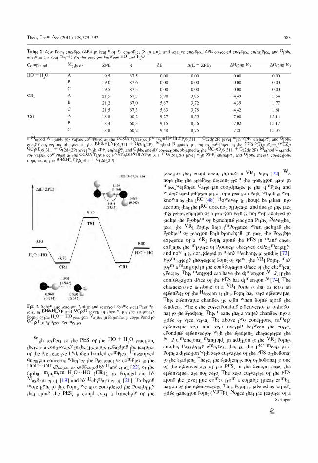
With respect to the PES of the HO ? H2O reaction,
there is a controversy in the literature regarding the features
of the pre-reactive hydrogen-bonded complex. Unresolved
question concerns whether the pre-reactive complex is the
HOH…OH species, as suggested by Hand et al. [22], or the
global minimum H2O…HO (CR1), as pointed out by
Masgrau et al. [19] and by Uchimaru et al. [21]. To bring
more light to this point, we also considered the possibility
that along the PES, it could exist a branching of the
reaction that could occur through a VRI point [72]. We
note that the steepest descent from the transition state in
mass-weighted Cartesian coordinates is the simplest and
widely used representation of a reaction path, which is well
known as the IRC [48]. However, it should be taken into
account that the IRC does not bifurcate, and due to this fact
this representation of a reaction path is not well adapted to
tackle the problem of branching reaction paths. Neverthe-
less, the VRI points gain importance when tackling the
problem of reaction path branching. In fact, the possible
existence of a VRI point along the PES in many cases
explains the mixture of products observed experimentally,
and now it is considered in many mechanistic studies [73].
From strictly theoretical point of view, the VRI points may
form a manifold in the configuration space of the chemical
species. This manifold can have the dimension N-2, if the
configuration space of the PES has dimension N [74]. The
characteristic attribute of a VRI point is that at least an
eigenpair of the Hessian at this point has zero eigenvalue.
This eigenvalue changes its sign when going along the
gradient, where the corresponding eigenvector is orthogo-
nal to the gradient. This means that a valley changes into a
ridge or vice versa. The above two conditions, namely
eigenvalue zero and zero overlap between the corre-
sponding eigenvector with the gradient, characterize the
N-2 dimensional manifold. In addition to the VRI points
another possibility emerges, that is, the IRC meets in a
point a direction with zero curvature of the PES orthogonal
to the gradient. There, the gradient is not orthogonal to one
of the eigenvectors of the PES, in the general case, the
eigenvalues are not zero. The zero curvature of the PES
along the level line comes from a suitable linear combi-
nation of the eigenvectors. This point is labeled as valley-
ridge transition point (VRTp). Notice that the features of a
Table 2 Zero-point energies (ZPE in kcal mol-1), entropies (S in a.u.), and relative energies, ZPE-corrected energies, enthalpies, and Gibbs
energies (in kcal mol-1) for the reaction between HO and H2O
Compound Methoda ZPE S DE D(E ? ZPE) DH(298 K) DG(298 K)
HO ? H2O A 19.5 87.5 0.00 0.00 0.00 0.00
B 19.0 87.6 0.00 0.00 0.00 0.00
C 19.5 87.5 0.00 0.00 0.00 0.00
CR1 A 21.5 67.3 -5.90 -3.85 -4.49 1.54
B 21.2 67.0 -5.87 -3.72 -4.39 1.77
C 21.5 67.3 -5.83 -3.78 -4.42 1.61
TS1 A 18.8 60.2 9.27 8.55 7.00 15.14
B 18.4 60.3 9.15 8.56 7.02 15.17
C 18.8 60.2 9.48 8.75 7.21 15.35
a Method A stands for values computed at the CCSD(T)/aug-cc-pVTZ//BH&HLYP/6-311 ? G(2df,2p) level with ZPE, enthalpy, and Gibbs
energy corrections obtained at the BH&HLYP/6-311 ? G(2df,2p); Method B stands for values computed at the CCSD(T)/aug-cc-pVTZ//
QCISD/6-311 ? G(2df,2p) level with ZPE, enthalpy, and Gibbs energy corrections obtained at the QCISD/6-311 ? G(2df,2p); Method C stands
for values computed at the CCSD(T)/aug-cc-pVQZ//BH&HLYP/6-311 ? G(2df,2p) level with ZPE, enthalpy, and Gibbs energy corrections
obtained at the BH&HLYP/6-311 ? G(2df,2p)
Fig. 2 Schematic reaction profile and selected geometrical parame-
ters, at BH&HLYP and QCISD levels of theory, for the stationary
points of the H2O ? HO reaction. Values in parenthesis correspond to
QCISD-optimized geometries
Theor Chem Acc (2011) 128:579–592 583
123

VRI point are stronger than those of a VRTp point. As will
see below, the present PES possesses this type of point.
In the PES associated with the present reaction mecha-
nism, the IRC curve leads directly from the transition state
TS1 to the corresponding deeper valley. The IRC curve
does not follow the crest of the ridge that leads to another
transition state, and it leads to one minimum that corre-
sponds to the global H2O…HO (CR1) minimum. In other
words, the located IRC leaves the asymmetric ridge, and it
goes to a minimum. However, this IRC path crosses an
equipotential line or contour line of the PES with null
curvature and meets with the border of the ridge region. At
the CASSCF level of theory, the VRTp is characterized by
a HO…HOH length of 1.458 A and a HO…H–OH angle of
151 degrees. Taking into account the CCSD(T) energies
computed at the CASSCF geometries, we predict that the
VRTp is located at 3.99 kcal mol-1 below TS1. The bor-
der of the ridge region is defined by the set of points such
that the projected Hessian matrix [(I - PT) H (I - P),
where the P matrix is build by the gradient direction and
the six zeros corresponding to translations and rotations]
has eigenvectors with null eigenvalues in addition to these
seven mentioned directions. These eigenvectors with null
eigenvalues are orthogonal to the gradient vector. Notice
that these eigenvectors are not eigenvectors of the full
Hessian matrix. At each point of the border line of the ridge
region, the direction of the equipotential line has null
curvature, and this direction is a linear combination of a
subset of eigenvectors of the full Hessian matrix. The
existence of a VRTp has important implications since both
the HOH…OH complex and the global minimum
H2O…HO (CR1) can be reached through this reaction.
3.3 The reaction between hydroxyl radical and a water
dimer
Figure 3 displays a schematic representation of the energy
profile of the reaction, along with the most relevant geo-
metrical parameters of the corresponding stationary points.
Table 3 contains their relative energies. For each of the
stationary points, we found two isomers differing in the
relative orientations of the dangling hydrogen atoms. These
two isomers are distinguished from each other by
appending the letter a, and the results displayed in Table 3
show that the two isomers of each stationary point are
almost energetically degenerate. For the sake of clarity, we
have drawn in Fig. 3 only one of these two isomers for
each stationary point, and the discussion along the text will
refer to only one of these isomers.
The potential energy profile schematized in Fig. 3 shows
that, starting at the (H2O)2 ? HO reactants, the reaction
begins with the formation of a hydrogen bond complex
CR2, for which we computed a binding energy of
7.42 kcal mol-1. This complex has a three-membered ring
structure where the two water molecules and the hydroxyl
radical are held together by three hydrogen bonds. The
calculated geometrical parameters compare quite well with
those reported recently by Tsuji et al. [75]. Then, the
reaction can proceed in two different ways, namely (a)
dissociating into the H2O…HO hydrogen bond complex
plus H2O and (b) proceeding through three different tran-
sition states. In this case, the exit channels are the same
species than in the reactant channels.
Regarding to path (a), the CR2a complex has a geo-
metric orientation that allows to dissociate directly into
Fig. 3 Schematic reaction
profile and selected geometrical
parameters, at BH&HLYP level
of theory, of the stationary
points of the (H2O)2 ? HO
reaction
584 Theor Chem Acc (2011) 128:579–592
123

H2O…HO ? H2O products, and the computed reaction
energy is -0.83 kcal mol-1. This process is tagged in the
present work as reaction 2, and it is very important from
atmospheric purposes as it contributes to the formation of
the hydrated hydroxyl radical in the atmosphere.
ðH2OÞ2 þ HO! CR2a ! H2O. . .HOþ H2O ð2Þ
Regarding to path (b), we found three different
elementary reactions. The first one occurs through TS2a,
which has a three-membered ring structure. This reaction
involves the homolitic breaking and forming of the O3–H
and H–O1 bonds, respectively, so that the hydroxyl radical
abstracts one hydrogen atom from a water molecule through
a HAT mechanism. Figure 3 shows that the hydrogen atom
being transferred is slightly closer (0.956 A) to the oxygen
atom of the water moiety than to the oxygen atom of the
radical (1.118 A) and that the transition state is stabilized by
two hydrogen bonds. From an energetic point of view, our
calculations predict this transition state to lie
5.58 kcal mol-1 above the energy of the reactants water
dimer plus hydroxyl radical (see Table 3). At this point, it is
worth comparing this value with the 8.75 kcal mol-1
computed for the transition state of the H2O ? HO
reaction described in the previous section (see Table 2).
Consequently, the addition of a second water molecule
produces a relative energy stabilization of the transition state
of 3.17 kcal mol-1, which can be attributed to the energy
stabilization produced by the formation of two hydrogen
bonds in TS2a. However, looking at the energy barrier
relative to the CR2a complex, the computed value is
13.07 kcal mol-1, which is even slightly larger than that
reported for the naked reaction (12.40 kcal mol-1, see
Table 2). Consequently, it seems that the possible catalytic
effect originated by the hydrogen bond stabilizations
occurring in the transition state is counteracted by the
enhanced stability of the pre-reactive complex, in a similar
way as reported by Allodi et al. [70] for the methane
oxidation by hydroxyl radical.
The second and third elementary reactions occur through
TS3 and TS4, which lie very high in energy (about
18 kcal mol-1 above the energy of the (H2O)2 ? HO
reactants; see Table 3; Fig. 3), so that it is expected that they
do not play any role. However, these elementary reactions
are interesting from a mechanistic point of view. The anal-
ysis of TS3 wave function indicates that the unpaired elec-
tron is mainly located over the hydroxyl radical moiety. It
does not participate at all in the process, and the reaction
mechanism involves a triple proton transfer process. In
TS4, the different atoms are oriented in such a way that the
unpaired electron of the hydroxyl radical moiety interacts
with one oxygen atom of a water molecule, so that it occurs a
transfer of an electron from this oxygen atom (O2) to the
oxygen of the hydroxyl radical (O1), and this originates a
simultaneous transfer of two protons (from O2 to O3 and
from O3 to O1, see Fig. 3). This elementary reaction cor-
responds to a proton coupled electron transfer mechanism
(pcet), and similar processes have been described recently in
the literature for the gas-phase oxidation of formic acid by
hydroxyl radical and for the same process assisted by a
single water molecule [25, 27, 76].
3.4 The reaction between hydroxyl radical and water
trimer
Figure 4 contains a schematic energy profile of the reaction
between (H2O)3 and HO radical, along with the most rel-
evant geometrical parameters of the main stationary points.
Table 4 contains the relative energies. Figure 4 shows that
the reaction begins with the formation of a complex
between the water trimer and the hydroxyl radical (CR3),
with a computed binding energy of 4.45 kcal mol-1. This
complex retains the three-membered ring structure of the
Table 3 Zero-point energies (ZPE in kcal mol-1), entropies (S in a.u.), and relative energies, ZPE-corrected energies, enthalpies, and Gibbs
energies (in kcal mol-1) for the reaction between HO and (H2O)2
Compound ZPE S DE D(E ? ZPE) DH(298 K) DG(298 K)
H2O…H2O ? OH 35.7 111.9 0.00 0.00 0.00 0.00
H2O…HO ? H2O 35.5 112.3 -0.66 -0.83 -0.96 -1.07
CR2 38.5 79.7 -10.28 -7.42 -8.67 0.93
CR2a 38.1 77.9 -9.94 -7.49 -9.03 1.12
TS2 35.5 76.2 6.27 6.06 4.28 14.95
TS2a 35.4 76.7 5.85 5.58 3.86 14.36
TS3 34.8 66.9 18.86 18.03 14.90 28.31
TS3a 34.7 67.0 18.45 17.52 14.41 27.80
TS4 36.2 67.7 17.79 18.29 15.38 28.55
TS4a 35.8 68.2 17.60 17.74 14.90 27.94
Values computed at the CCSD(T)/aug-cc-pVTZ//BH&HLYP/6-311 ? G(2df,2p) level with ZPE, enthalpy, and Gibbs energy corrections
obtained at the BH&HLYP/6-311 ? G(2df,2p)
Theor Chem Acc (2011) 128:579–592 585
123

water trimer, and the hydrogen atom of the radical interacts
with one of the oxygen atoms of (H2O)3 cluster. As in the
previous section, for each stationary point there are three
isomers differing in the relative orientations of the dangling
hydrogen. They are almost degenerate in energy and, for
the sake of clarity, we will consider the lowest energy one
along the discussion.
The reaction goes on through TS51 to form the CR4
complex, which has a four-membered ring structure (see
Fig. 4). It is stabilized by four hydrogen bonds, and it lies
8.57 kcal mol-1 below the sum of the energies of the water
trimer and the hydroxyl radical reactants. Our computed
geometrical parameters compare quite well with those
reported recently by Tsuji et al. [75]. After this complex,
the reaction can proceed through three different reaction
paths. The three elementary reactions have the same elec-
tronic features as described in the previous section for the
reaction of the water dimer with the hydroxyl radical, and
they will be not discussed here. The first reaction (HAT
process) goes through TS6, and it involves the homolytic
breaking and forming of the O4-H and H-O1 bonds,
respectively. Our calculations predict this transition state to
lie 5.27 kcal mol-1 above the reactants energy, and the
computed energy barrier is 13.84 kcal mol-1 relative to
CR4. As discussed in the previous section, TS6 lies lower
in energy, relative to the separate reactants, than TS1 of the
Fig. 4 Schematic reaction
profile and selected geometrical
parameters, at BH&HLYP level
of theory, of the stationary
points of the (H2O)3 ? HO
reaction. The reaction products
are the same species than the
reactants, and therefore they are
not explicitly drawn
Table 4 Zero-point energies (ZPE in kcal mol-1), entropies (S in a.u.), and relative energies, ZPE-corrected energies, enthalpies, and Gibbs
energies (in kcal mol-1) for the reaction between HO and (H2O)3
Compound ZPE S DE D(E ? ZPE) DH(298 K) DG(298 K)
(H2O)3 ? OH 52.9 122.6 0.00 0.00 0.00 0.00
(H2O)2…HO ? H2O 52.5 124.7 4.71 4.23 4.25 3.61
CR3a 54.8 99.3 -6.27 -4.45 -4.86 2.07
TS5a 53.9 99.9 -4.55 -3.55 -4.03 2.74
CR4 55.3 93.4 -10.91 -8.57 -9.42 -0.72
TS6 52.3 89.2 5.90 5.27 3.87 13.82
TS6a 52.1 90.4 6.38 5.53 4.24 13.83
TS6b 52.2 89.8 6.25 5.52 4.18 13.94
TS7 50.1 78.4 14.63 11.78 8.86 22.03
TS8 51.3 78.6 17.45 15.85 13.04 26.14
Values computed at the CCSD(T)/aug-cc-pVTZ//BH&HLYP/6-311 ? G(2df,2p) level with ZPE, enthalpy and Gibbs energy corrections
obtained at the BH&HLYP/6-311 ? G(2df,2p)a For the enthalpic, and Gibbs energy corrections, see Footnote 1
1 The CR3 ? CR4 path is very flat and we have failed to find TS5 at
BH&HLYP level of theory We have optimized it, and CR3 too, using
the B3LYP functional and their corresponding ZPE, entropy and
enthalpy corrections have been employed in this case.
586 Theor Chem Acc (2011) 128:579–592
123
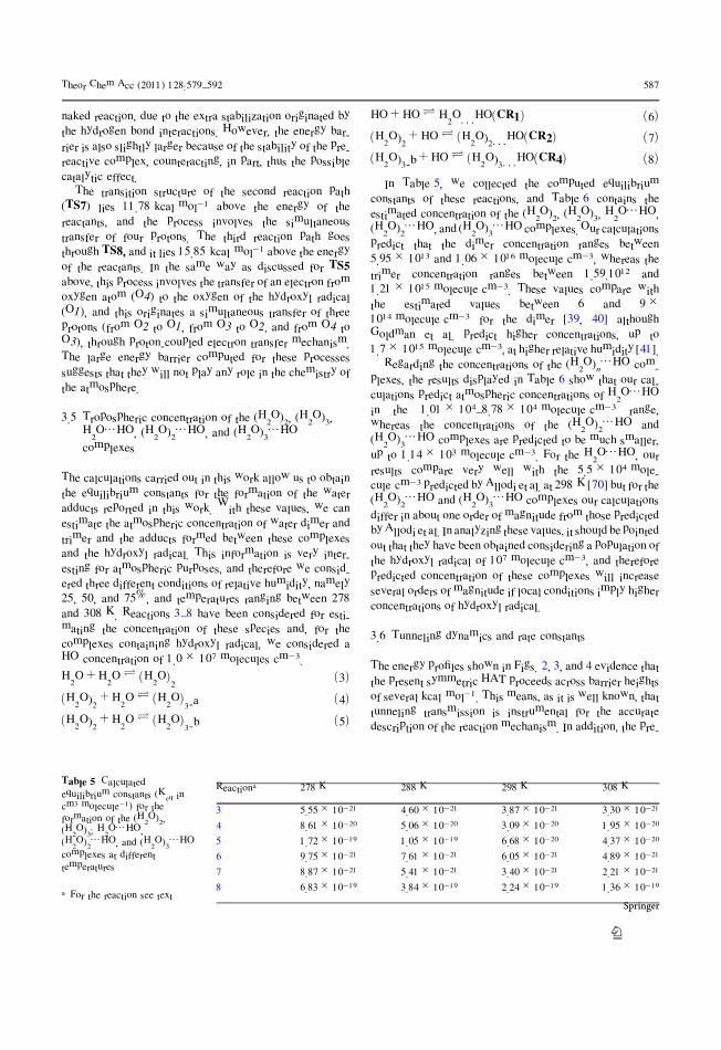
naked reaction, due to the extra stabilization originated by
the hydrogen bond interactions. However, the energy bar-
rier is also slightly larger because of the stability of the pre-
reactive complex, counteracting, in part, thus the possible
catalytic effect.
The transition structure of the second reaction path
(TS7) lies 11.78 kcal mol-1 above the energy of the
reactants, and the process involves the simultaneous
transfer of four protons. The third reaction path goes
through TS8, and it lies 15.85 kcal mol-1 above the energy
of the reactants. In the same way as discussed for TS5
above, this process involves the transfer of an electron from
oxygen atom (O4) to the oxygen of the hydroxyl radical
(O1), and this originates a simultaneous transfer of three
protons (from O2 to O1, from O3 to O2, and from O4 to
O3), through proton-coupled electron transfer mechanism.
The large energy barrier computed for these processes
suggests that they will not play any role in the chemistry of
the atmosphere.
3.5 Tropospheric concentration of the (H2O)2, (H2O)3,
H2O…HO, (H2O)2…HO, and (H2O)3…HO
complexes
The calculations carried out in this work allow us to obtain
the equilibrium constants for the formation of the water
adducts reported in this work. With these values, we can
estimate the atmospheric concentration of water dimer and
trimer and the adducts formed between these complexes
and the hydroxyl radical. This information is very inter-
esting for atmospheric purposes, and therefore we consid-
ered three different conditions of relative humidity, namely
25, 50, and 75%, and temperatures ranging between 278
and 308 K. Reactions 3–8 have been considered for esti-
mating the concentration of these species and, for the
complexes containing hydroxyl radical, we considered a
HO concentration of 1.0 9 107 molecules cm-3.
H2Oþ H2O� ðH2OÞ2 ð3Þ
ðH2O)2 þ H2O� ðH2OÞ3-a ð4Þ
ðH2O)2 þ H2O� ðH2OÞ3-b ð5Þ
HOþ HO� H2O. . .HOðCR1Þ ð6Þ
ðH2O)2 þ HO� ðH2O)2. . .HOðCR2Þ ð7Þ
ðH2O)3-bþ HO� ðH2O)3. . .HOðCR4Þ ð8Þ
In Table 5, we collected the computed equilibrium
constants of these reactions, and Table 6 contains the
estimated concentration of the (H2O)2, (H2O)3, H2O…HO,
(H2O)2…HO, and (H2O)3…HO complexes. Our calculations
predict that the dimer concentration ranges between
5.95 9 1013 and 1.06 9 1016 molecule cm-3, whereas the
trimer concentration ranges between 1.59Á1012 and
1.21 9 1015 molecule cm-3. These values compare with
the estimated values between 6 and 9 9
1014 molecule cm-3 for the dimer [39, 40] although
Goldman et al. predict higher concentrations, up to
1.7 9 1015 molecule cm-3, at higher relative humidity [41].
Regarding the concentrations of the (H2O)n…HO com-
plexes, the results displayed in Table 6 show that our cal-
culations predict atmospheric concentrations of H2O…HO
in the 1.01 9 104–8.78 9 104 molecule cm-3 range,
whereas the concentrations of the (H2O)2…HO and
(H2O)3…HO complexes are predicted to be much smaller,
up to 1.14 9 103 molecule cm-3. For the H2O…HO, our
results compare very well with the 5.5 9 104 mole-
cule cm-3 predicted by Allodi et al. at 298 K [70] but for the
(H2O)2…HO and (H2O)3…HO complexes our calculations
differ in about one order of magnitude from those predicted
byAllodi et al. In analyzing these values, it should be pointed
out that they have been obtained considering a population of
the hydroxyl radical of 107 molecule cm-3, and therefore
predicted concentration of these complexes will increase
several orders of magnitude if local conditions imply higher
concentrations of hydroxyl radical.
3.6 Tunneling dynamics and rate constants
The energy profiles shown in Figs. 2, 3, and 4 evidence that
the present symmetric HAT proceeds across barrier heights
of several kcal mol-1. This means, as it is well known, that
tunneling transmission is instrumental for the accurate
description of the reaction mechanism. In addition, the pre-
Table 5 Calculated
equilibrium constants (Keq in
cm3 molecule-1) for the
formation of the (H2O)2,
(H2O)3; H2O…HO,
(H2O)2…HO, and (H2O)3…HO
complexes at different
temperatures
a For the reaction see text
Reactiona 278 K 288 K 298 K 308 K
3 5.55 9 10-21 4.60 9 10-21 3.87 9 10-21 3.30 9 10-21
4 8.61 9 10-20 5.06 9 10-20 3.09 9 10-20 1.95 9 10-20
5 1.72 9 10-19 1.05 9 10-19 6.68 9 10-20 4.37 9 10-20
6 9.75 9 10-21 7.61 9 10-21 6.05 9 10-21 4.89 9 10-21
7 8.87 9 10-21 5.41 9 10-21 3.40 9 10-21 2.21 9 10-21
8 6.83 9 10-19 3.84 9 10-19 2.24 9 10-19 1.36 9 10-19
Theor Chem Acc (2011) 128:579–592 587
123

reactive complexes also play a determining role in the form
of interferences (resonances) that may be reflected in the
transmission factor.
Quantifying the above tunneling, resonance features
requires performing some sort of quantum dynamics study.
The present systems involve a large number of coupled
degrees of freedom, so that solving exactly the nuclear
dynamics problem proves as a daunting task. To alleviate
this problem, some of the authors recently developed a
quantum dynamics methodology, based on restricting the
molecular motion to the reaction path, so that the compu-
tational requirements are reduced to a minimal amount.
Specific details of the methodology are given elsewhere
[59]. Here, it suffices to understand that a properly defined
wavepacket has been time evolved along the reaction
profile, as provided by the reaction path, and the energy-
dependent transmission factor is computed afterward, by
means of a suitable Fourier transform of a reactants auto-
correlation function. Results of the tunneling dynamics are
shown below, restricted to one- and two-water cases, for
the sake of deeming clearer the ensuing comparisons. Since
in all the cases, the HAT mechanism is energetically
favored (see Figs. 2, 3, 4), we limited ourselves to it. This
process has proven to have an important tunneling contri-
bution for reaction 1 as it has been pointed out in previous
studies of the literature [19, 21].
Figure 5 shows the energy-dependent transmission
factor, for the reaction between OH radical and one water
molecule. Fixed-mass calculations are compared with
variable mass, since this comparison provides interesting
clues on the role played by perpendicular modes in the
reaction dynamics. Fixed-mass calculations show an
important tunneling contribution to transmission, as well
as antitunneling at energies above the barrier. These are
rather expected results, considering the fact that, in the
present process, a light atom, hydrogen, is transmitted
between two heavy centers (H2O and O). In addition,
inspection of the potential energy profile along the IRC
clearly tells that one should expect tunneling to be
important, since the barrier develops a rather thin profile,
becoming thinner as energy is increased. This has been
done by considering the geometries and frequencies
obtained at BH&HLYP/6-311 ? G(2df,2p) level of theory
and the energies computed at CCSD(T)/aug-cc-pVTZ
level of theory. However, tunneling appears even more
enhanced, when one considers variable–mass results. One
might then say that the influence of perpendicular modes
is, rather surprisingly, to enhance reactivity below the
Table 6 Estimated tropospheric concentrations (in molecule cm-3) of the (H2O)2, (H2O)3, H2O…HO, (H2O)2…HO, and (H2O)3…HO com-
plexes at different relative humidities (RH) and temperatures (T)
T RH = 25% RH = 50% RH = 75%
H2O (H2O)2 (H2O)3 H2O (H2O)2 (H2O)3 H2O (H2O)2 (H2O)3
278 1.04 9 1017 5.95 9 1013 1.59 9 1012 2.07 9 1017 2.38 9 1014 1.27 9 1013 3.11 9 1017 5.36 9 1014 4.30 9 1013
288 1.92 9 1017 1.70 9 1014 5.08 9 1012 3.84 9 1017 6.79 9 1014 4.06 9 1013 5.76 9 1017 1.53 9 1015 1.37 9 1014
298 3.48 9 1017 4.68 9 1014 1.59 9 1013 6.95 9 1017 1.87 9 1015 1.27 9 1014 1.04 9 1018 4.21 9 1015 4.29 9 1014
308 5.99 9 1017 1.18 9 1015 4.47 9 1013 1.20 9 1018 4.73 9 1015 3.58 9 1014 1.80 9 1018 1.06 9 1016 1.21 9 1015
H2O…HO (H2O)2…HO (H2O)3…HO H2O…HO (H2O)2…HO (H2O)3…HO H2O…HO (H2O)2…HO (H2O)3…HO
278 1.01 9 104 9.28 7.24 2.02 9 104 3.71 9 101 5.79 9 101 3.03 9 104 8.35 9 101 1.96 9 102
288 1.46 9 104 1.52 9 101 1.32 9 101 2.92 9 104 6.08 9 101 1.05 9 102 4.39 9 104 1.37 9 102 3.55 9 102
298 2.10 9 104 2.49 9 101 2.44 9 101 4.21 9 104 9.95 9 101 1.95 9 102 6.31 9 104 2.24 9 102 6.58 9 102
308 2.93 9 104 3.87 9 101 4.21 9 102 5.85 9 104 1.55 9 102 3.36 9 102 8.78 9 104 3.48 9 102 1.14 9 103
These estimations have been done according Eqs. 3–8
The concentration of the hydroxyl radical employed for the formation of the (H2O)n…HO complexes is 1.0 9 107 molecules cm-3
Fig. 5 Calculated transmission factor for the reaction between HO
and H2O. The vertical black line corresponds to the classical energy
barrier
588 Theor Chem Acc (2011) 128:579–592
123

potential energy barrier. This is in contrast to numerous
previous studies on tunneling, where the inclusion of more
degrees of freedom normally inhibits tunneling. In addi-
tion, oscillations in the transmission factor, as energy is
increased, are more intense in the variable–mass case,
indicating that interference phenomena are enhanced by
the inclusion of perpendicular modes. This is a suggestive
result, whose origin may be traced back to the symmetric
character of the present reactions and their Heavy–Light–
Heavy nature.
Tunneling contribution to reaction, for the reaction
between OH and two water molecules, is analyzed in
Fig. 6. Q–RPH transmission factor, as a function of energy,
is shown for cis and trans configurations of the water
dimer. Results show, first, that cis–trans differences are
only an energy shift, the qualitative shape being fairly
equal. This is the reason why we do not show results for all
the isomers in all cases, limiting ourselves to this case.
Second, the contribution to tunneling is again remarkable,
but the most outstanding feature is the oscillating nature of
the transmission factor in the threshold and post-threshold
regions. These oscillations are much more pronounced than
the previous case. It is clearly an influence of the deeper
CR1 well (ca. 7.5 kcal mol-1 for the two-water case,
versus ca. 3.8 kcal mol-1 well depth for the one-water
reaction).
Further comparison between one- and two-water reac-
tions evidences that, whereas tunneling is of similar
importance for both reactions, antitunneling is remarkably
larger in the one-water case. It is shown by the slower trend
to unity, in the large energy regime, when comparing
Figs. 5 and 6. This feature is interesting, since this large
antitunneling appears only in the variable mass case of the
one-water reaction, i.e., only when the perpendicular
modes to reaction are taken into account. The primary
conclusion is then that energy sequestering (from that
available to reaction) is more effective for one-water than
for two-water reactions. The explanation for such behavior
might resort to a kind of entropic effect: energy flow
concentrates more easily in a small number of non-reacting
modes than in a larger number of them. In addition, the
higher symmetry content, of the two-water TS, also sug-
gests a much higher difficulty in concentrating the energy
flow in non-reacting modes, when compared to the one-
water reaction.
Once analyzed the behavior of the transmission factor
along the reaction path, we computed the rate constant of
the reaction. To do this, we considered the reactions to
occur at 1 atm. of pressure, and we applied the steady-state
approximation to the pre-reactive complex, and the rate
constant is given by Eq. 9.
kTOT ¼ Keq Á k2 Á jtun ð9Þ
where Keq is the equilibrium constant, k2 is the
unimolecular rate constant, and jtun is the tunneling
contribution that has been computed by Eq. 10.
jtunðTÞ ¼
R10TðEÞ exp À E
kBT
� �
dE
R1Vbexp À E
kBT
� �
dEð10Þ
We have to mention here that applying Eq. 9 is just a
limiting case, and the effect of low pressures would require
a different treatment that is beyond the scope of the present
work.
In Table 7, we collected the computed rate constant. For
the H2O ? HO reaction, our computed values range
between 2.76 9 10-17 and 6.04 9 10-17 cm3 mole-
cule-1 s-1 in the 200–400 K range of temperatures and
compare very well with the results reported by Masgrau
et al. [19] and Uchimaru et al. [21], the differences with the
last one being mainly attributed to the fact that they use a
reaction profile beginning in the reactants without taking
into account the pre-reactive complex. It is worth noting
here the importance of the tunneling contribution, mainly
at low temperatures, as it was pointed out in previous
works on this reaction [19, 21].
Although for the case of the reaction between HO and
(H2O)2 we report rate constants, we pointed out in a
previous section that the pre-reactive complex CR2 dis-
sociates into H2O…HO ? H2O and therefore, we can
conclude that the reaction through TS2 would not occur at
all.
The reaction between hydroxyl radical and water trimer
is much more complex, and k2 is computed using Eq. 11
according to the unified statistical model [77], and the
Fig. 6 Calculated transmission factor through TS2 and TS2a for the
reaction between HO and (H2O)2. The vertical black lines correspond
to the classical energy barriers
Theor Chem Acc (2011) 128:579–592 589
123

1
k2¼
1
kTS5þ
1
kTS6ð11Þ
results displayed in Table 5 show that in this case, the
reaction is much faster than reaction 1, with values ranging
between 1.25 9 10-13 and 8.33 9 10-16 cm3 mole-
cule-1 s-1 in the 200–400 K range of temperatures. Here,
it is important to note that the tunneling contribution is
very similar to those occurring in reaction 1.
4 Conclusions
The reactions between HO and (H2O)n (n = 1, 3) have
been investigated using high-level theoretical methods, and
the results obtained allow us to highlight the following
points.
Regarding the water dimer and trimer, our calculations
predict a binding energy of 2.86 kcal mol-1 for (H2O)2relative to H2O ? H2O and 7.67 kcal mol-1 for (H2O)3relative to (H2O)2 ? H2O.
Our calculations predict atmospheric concentration for
the (H2O)2 complex in the range between 5.95 9 1013 and
1.06 9 1016 molecule cm-3 and for the (H2O)3 complex in
the range between 1.59 9 1012 and 1.21 9 1015 mole-
cule cm-3; depending on the atmospheric conditions of
relative humidity and temperature. For the H2O…HO
complex, we predict atmospheric concentrations in the
1.01 9 104 – 8.78 9 104 molecule cm-3, depending on
the atmospheric conditions and considering a hydroxyl
radical population of 107 molecule cm-3. The concentra-
tion of the (H2O)2…HO and (HO)3…HO is predicted to be
about two orders of magnitude smaller.
All the reactions considered are symmetric, and they
begin with the formation of a pre-reactive hydrogen-bon-
ded complex.
For the reaction of hydroxyl radical with a single water
molecule, our calculations predict that the pre-reactive
hydrogen-bonded complex CR1 has a binding energy of
3.78 kcal mol-1, whereas the transition state lies
12.53 kcal mol-1 above CR1. Very interestingly, we
found a VRI point along the reaction path, which is ener-
getically located close to 4 kcal mol-1 below the transition
state, which allows branching the reaction path. The
computed rate constant for this reaction range between
2.76 9 10-17 and 6.04 9 10-17 cm3 molecule-1 s-1 in
the 200–400 K range of temperatures.
For the reaction between hydroxyl radical and water
dimer, our calculations predict the pre-reactive complexes
(CR2 and CR2a) to have binding energies close to
7.5 kcal mol-1. Then, the reaction can proceed in two
different ways: (a) dissociating directly into the H2O…HO
Table 7 Computed rate
constants for the reaction
between hydroxyl radical and
water, water dimer, and water
trimer
Keq are in cm3 molecule-1, K2are in s-1, then total constants
KTOT are in
cm3 molecule-1 s-1
stun is the tunneling correction
K2 stands for kTS1, kTS2, kTS5,and kTS6, respectivelyastun applies to reaction
through kTS6
Reaction OH ? H2O
Temperature Keq kTS1 stun KTOT
200 1.72 9 10-19 5.09 9 10-6 3.15 9 107 2.76 9 10-17
250 2.19 9 10-20 1.32 9 10-2 5.33 9 104 1.54 9 10-17
298 6.05 9 10-21 2.04 1.40 9 103 1.73 9 10-17
350 2.32 9 10-21 9.92 9 10 1.28 9 102 2.95 9 10-17
400 1.21 9 10-21 1.58 9 103 3.16 9 101 6.04 9 10-17
Reaction OH ? (H2O)2
Temperature Keq kTS2 stun KTOT
200 1.90 9 10-17 2.24 9 10-4 1.05 9 107 4.47 9 10-14
250 2.59 9 10-19 4.04 9 10-1 2.78 9 104 2.91 9 10-15
298 1.57 9 10-20 4.98 9 10 9.47 9 102 7.40 9 10-16
350 1.77 9 10-21 2.05 9 103 1.02 9 102 3.70 9 10-16
400 3.70 9 10-22 2.9 9 104 2.76 9 10 2.97 9 10-16
Reaction OH ? (H2O)3
Temperature Keq kTS5 kTS6 stuna KTOT
200 4.50 9 10-16 6.14 9 1011 1.24 9 10-5 2.24 9 107 1.25 9 10-13
250 4.40 9 10-18 1.20 9 1012 3.89 9 10-2 4.01 9 104 6.86 9 10-15
298 2.24 9 10-19 1.89 9 1012 6.95 1.11 9 103 1.73 9 10-15
350 2.27 9 10-20 2.73 9 1012 3.83 9 102 1.08 9 102 9.37 9 10-16
400 4.45 9 10-21 3.56 9 1012 6.76 9 103 2.77 9 10 8.33 9 10-16
590 Theor Chem Acc (2011) 128:579–592
123

complex and H2O, requiring an energy of ca 6.6 kcal -
mol-1 and (b) proceeding through three different elemen-
tary reactions. In this case, the more favorable path occurs
through TS2a, which is predicted to lie 13.07 kcal mol-1
above CR2a, and it involves a hydrogen atom transfer
mechanism. The high energy barrier computed for TS2a
along with the rate constant computed for this elementary
reaction indicated that the reaction between HO and (H2O)2will produce H2O…HO and H2O, and it will contribute to
the atmospheric formation of hydrated hydroxyl radical,
which has an important significance in the chemistry of the
atmosphere.
The reaction with hydroxyl radical and water trimer
begins with the addition of the HO radical to the three-
membered ring of the water trimer forming the CR3
complex. Then, it occurs a geometrical rearrangement to
form the four-membered ring CR4 complex, which is
computed to be 8.57 kcal mol-1 more stable than the
reactants. Then, the reaction can go on through three dif-
ferent reactions paths. The more favorable one occurs
through TS6, which is predicted to lie 5.27 kcal mol-1
above the separate reactants, and it involves a hydrogen
atom transfer mechanism. This reaction is predicted to be
faster than the reaction between hydroxyl radical and one
water molecule, which has a rate constant in the range
1.25 9 10-13 – 8.33 9 10-16 cm3 molecule-1 s-1 in the
200–400 K range of temperatures, a fact that is attributed
to the complexity of the whole reaction path.
For all the reactions considered, the transmission via
tunneling effect is found to be very important, especially at
low temperatures. Other features that also appear to be
relevant from a dynamical point of view and that deserve
more studies are the enhancement of tunneling due to the
inclusion of perpendicular modes via the Q-RPH, the
remarkable antitunneling for the reaction between HO and
H2O, and the oscillations in the transmission factor for the
reaction of the HO radical and (H2O)2. The latter is
attributed to an increment of resonances due to the deeper
well of the corresponding CR1 compared with the
HO ? H2O case.
Acknowledgments This research has been supported by the Gen-
eralitat de Catalunya (Grant 2009SGR01472) and the Spanish Di-
reccion General de Investigacion Cientıfica y Tecnica (DGYCIT,
grants CTQ2008-06536/BQU and CTQ2008-02856/BQU). The cal-
culations described in this work were carried out at the Centre de
Supercomputacio de Catalunya (CESCA), at the Computational
Center of CTI–CSIC, and at the cluster of workstations of our group.
Antoni Aguilar-Mogas and Marc Caballero gratefully thank to Min-
isterio de Ciencia e Innovacion for a predoctoral fellowship. Javier
Gonzalez and Miquel Torrent-Sucarrat acknowledge CSIC for a JAE-
DOC contract.
References
1. Wayne RP (2000) Chemistry of atmospheres, 3rd edn. Oxford
University Press, Oxford
2. Wennberg PO, Hanisco TF, Jaegle L, Jacob DJ, Hintsa EJ,
Lanzendorf EJ, Anderson JG, Gao RS, Keim ER, Donnelly SG,
Negro LAD, Fahey DW, McKeen SA, Salawitch RJ, Webster
CR, May RD, Herman RL, Proffitt MH, Margitan JJ, Atlas EL,
Schauffler SM, Flocke F, McElroy CT, Bui TP (1998) Science
279:49–53
3. Monks PS (2005) Gas-phase radical chemistry in the troposphere.
Chem Soc Rev 34:376–395
4. Jaegle L, Jacob DJ, Brune WH, Wennberg PO (2001) Atmos
Environ 35:469–489
5. Hofzumahaus A, Rohrer F, Lu KD, Bohn B, Brauers T, Chang
CC, Fuchs H, Holland F, Kita K, Kondo Y, Li X, Lou SR, Shao
M, Zeng LM, Wahner A, Zhang YH (2009) Science
324(5935):1702–1704. doi:10.1126/science.1164566
6. Mansergas A, Anglada JM (2007) ChemPhysChem 8:1534–1539
7. Jacob DJ (2000) Atmos Environ 34(12–14):2131–2159
8. Chameides WL, Davis DD (1982) J Geophys Res Oceans
Atmospheres 87(NC7):4863–4877
9. Hanson DR, Burkholder JB, Howard CJ, Ravishankara AR
(1992) J Phys Chem 96(12):4979–4985
10. Kregel KC, Zhang HJ (2007) Am J Physiol Regul Integr Comp
Physiol 292(1):R18–R36
11. Pryor WA, Houk KN, Foote CS, Fukuto JM, Ignarro LJ,
Squadrito GL, Davies KJ (2006) Am J Physiol Regul Integr
Comp Physiol 291(3):R491–R511
12. Fridovich I (1998) J Exp Biol 201(Pt 8):1203–1209
13. Kehrer JP (2000) Toxicology 149(1):43–50
14. Cooper WJ, Cramer CJ, Martin NH, Mezyk SP, O’Shea KE, von
Sonntag C (2009) Chem Rev 109(3):1302–1345. doi:
10.1021/cr078024c
15. Sein MM, Golloch A, Schmidt TC, von Sonntag C (2007)
ChemPhysChem 8(14):2065–2067
16. Lesko TM, Colussi AJ, Hoffmann MR (2004) J Am Chem Soc
126:4432–4436
17. Sehested K, Corfitzen H, Holcman J, Hart EJ (1998) J Phys Chem
A 102:2667–2672
18. Dubey MK, Mohrschladt R, Donahue NM, Anderson JG (1997) J
Phys Chem A 101(8):1494–1500
19. Masgrau L, Gonzalez-Lafont A, Lluch JM (1999) J Phys Chem A
103(8):1044–1053
20. Masgrau L, Gonzalez-Lafont A, Lluch JM (1999) J Comput
Chem 20(16):1685–1692
21. Uchimaru T, Chandra AK, Tsuzuki S, Sugie M, Sekiya A (2003)
J Comput Chem 24:1538–1548
22. Hand MR, Rodriquez CF, Williams IH, Balint-Kurti GG (1998) J
Phys Chem A 102(29):5958–5966
23. Basch H, Hoz S (1997) J Phys Chem A 101(24):4416–4431
24. Deyerl HJ, Luong AK, Clements TG, Continetti RE (2000)
Faraday Discuss 115:147–160
25. Olivella S, Anglada JM, Sole A, Bofill JM (2004) Chem Eur J
10:3404–3410. doi:10.1002/chem.200305714
26. Vohringer-Martinez E, Hansmann B, Hernandez H, Francisco JS,
Troe J, Abel B (2007) Science 315(5811):497–501
27. Anglada JM, Gonzalez J (2009) ChemPhysChem 10(17):3034–
3045. doi:10.1002/cphc.200900387
28. Luo Y, Maeda S, Ohno K (2009) Chem Phys Lett 469:57–61
29. Aloisio S, Francisco JS, Friedl RR (2000) J Phys Chem A
104:6597–6601
Theor Chem Acc (2011) 128:579–592 591
123
30. Zhu RS, Lin MC (2002) Chem Phys Lett 354(3–4):217–226
31. Anglada JM, Aplincourt P, Bofill JM, Cremer D (2002) Chem-
PhysChem 2:215–221
32. Crehuet R, Anglada JM, Bofill JM (2001) Chem Eur J
7(10):2227–2235
33. Neeb P, Sauer F, Horie O, Moortgat GK (1997) Atmos Environ
31(10):1417–1423
34. Gonzalez J, Torrent-Sucarrat M, Anglada JM (2010) Phy-
sChemChemPhys 12(9):2116–2125. doi:10.1039/b916659a
35. Bahnson BJ, Colby TD, Chin JK, Goldstein BM, Klinman JP
(1997) Proc Natl Acad Sci USA 94(24):12797–12802
36. Giese K, Petkovic M, Naundorf H, Kuhn O (2006) Phys Rep Rev
Sect Phys Lett 430(4):211–276. doi:10.1016/j.physrep.2006.
04.005
37. Guallar V, Gherman BF, Miller WH, Lippard SJ, Friesner RA
(2002) J Am Chem Soc 124(13):3377–3384. doi:10.1021/
ja0167248
38. Makri N (1999) Annual Rev Phys Chem 50:167–191
39. Pfeilsticker K, Lotter A, Peters C, Bosch H (2003) Science
300(5628):2078–2080
40. Dunn ME, Pokon EK, Shields GC (2004) J Am Chem Soc
126:2647–2653
41. Goldman N, Fellers RS, Leforestier C, Saykally RJ (2001) J Phys
Chem A 105(3):515–519
42. Becke AD (1993) J Chem Phys 98:1372
43. Frisch MJ, Pople JA, Binkley JS (1984) J Chem Phys
80:3265–3269
44. Hehre WJ, Radom L, Schleyer PvR, Pople JA (1986) Ab initio
molecular orbital theory. Wiley, New York, pp 86–87
45. Ishida K, Morokuma K, Kormornicki A (1977) J Chem Phys
66:2153
46. Gonzalez C, Schlegel HB (1989) J Chem Phys 90:2154
47. Gonzalez C, Schlegel HB (1990) J Phys Chem 94:5523
48. Fukui K (1970) J Phys Chem 74(23):4161
49. Cizek J (1969) Adv Chem Phys 14:35
50. Barlett RJ (1989) J Phys Chem 93:1963
51. Pople JA, Krishnan R, Schlegel HB, Binkley JS (1978) Int J
Quant Chem XIV:545–560
52. Pople JA, Head-Gordon M, Raghavachari K (1989) J Chem Phys
90(8):4635–4636
53. Dunning THJ (1989) J Chem Phys 90:1007
54. Kendall RA, Dunning TH, Harrison RJ (1992) J Chem Phys
96(9):6796–6806
55. Pople JA, Head-Gordon M, Raghavachari K (1987) J Chem Phys
87:5968
56. Roos BO (1987) Adv Chem Phys 69:399
57. Frisch MJ, Trucks GW, Schlegel HB, Scuseria GE, Robb MA,
Cheeseman JA Jr, Montgomery J, Vreven T, Kudin KN, Burant
JC, Millam JM, Iyengar SS, Tomasi J, Barone V, Mennucci B,
Cossi M, Scalmani G, Rega N, Petersson GA, Nakatsuji H, Hada
M, Ehara M, Toyota K, Fukuda R, Hasegawa J, Ishida M, Nak-
ajima T, Honda Y, Kitao O, Nakai H, Klene M, Li X, Knox JE,
Hratchian HP, Cross JB, Adamo C, Jaramillo J, Gomperts R,
Stratmann RE, Yazyev O, Austin AJ, Cammi R, Pomelli C,
Ocherski JW, Ayala PY, Morokuma K, Voth GA, Salvador P,
Dannenberg JJ, Zakrzewski VG, Dapprich S, Daniels AD, Strain
MC, Farkas O, Malick DK, Rabuck AD, Raghavachari K,
Foresman JB, Ortiz JV, Cui Q, Baboul AG, Clifford S, Cio-
slowski J, Stefanov BB, Liu G, Liashenko A, Piskorz P, Ko-
maromi I, Martin RL, Fox DJ, Keith T, Al-Laham MA, Peng CY,
Nanayakkara A, Challacombe M, Gill PMW, Johnson B, Chen
W, Wong MW, Gonzalez C, Pople JA (2004) Gaussian 03,
revision C.01 edn. Gaussian, Inc., Wallingford, CT
58. Schmidt MW, Baldridge KK, Boatz JA, Elbert ST, Gordon MS,
Jensen JH, Koseki S, Matsunaga N, Nguyen KA, Su SJ, Windus
TL, Dupuis M, Montgomery JA (1993) Gamess 2004. J Comput
Chem 14:1347–1363
59. Gonzalez J, Gimenez X, Bofill JM (2009) J Chem Phys
131(5):054108. doi:10.1063/1.3194135
60. Gonzalez J, Gimenez X, Bofill JM (2001) J Phys Chem A
105(20):5022–5029. doi:10.1021/jp003793k
61. Gonzalez J, Gimenez X, Bofill JM (2007) J Comput Chem 28
(13):2111–2121. doi:10.1002/jcc.20729
62. Gonzalez J, Gimenez X, Bofill JM (2007) J Comput Chem
28(13):2102–2110. doi:10.1002/jcc.20728
63. Gonzalez J, Gimenez X, Bofill JM (2004) Theor Chem Acc
112(2):75–83. doi:10.1007/s00214-004-0571-6
64. Askar A, Cakmak AS (1978) J Chem Phys 68(6):2794–2798
65. Klopper W, de Rijdt J, van Duijneveldt FB (2000) PhysChem-
ChemPhys 2(10):2227–2234
66. Zhou Z, Qu Y, Fu A, Du B, He F, Gao H (2002) Int J Quant
Chem 89:550–558
67. Cooper PD, Kjaergaard HG, Langford VS, McKinley AJ,
Quickenden TI, Schofield DP (2003) J Am Chem Soc
125(20):6048–6049
68. Engdahl A, Karlstrom G, Nelander B (2003) J Chem Phys
118(17):7797–7802
69. Ohshima Y, Sato K, Sumiyoshi Y, Endo Y (2005) J Am Chem
Soc 127(4):1108–1109
70. Allodi MA, Dunn ME, Livada J, Kirschner KN, Shields GC
(2006) J Phys Chem A 110(49):13283–13289
71. Soloveichik P, O’Donnell BA, Lester MI, Francisco JS, McCoy
AB (2010) J Phys Chem A 114(3):1529–1538. doi:10.1021/
jp907885d
72. Quapp W, Hirsch M, Heidrich D (1998) Theor Chem Acc
100(5–6):285–299
73. Ess DH, Wheeler SE, Iafe RG, Xu L, Celebi-Olcum N, Houk KN
(2008) Angew Chem Int Ed Engl 47(40):7592–7601. doi:10.1002/
anie.200800918
74. Valtazanos P, Ruedenberg K (1986) Theor Chim Acta 69(4):
281–307
75. Tsuji K, Shibuya K (2009) J Phys Chem A 113(37):9945–9951.
doi:10.1021/jp903648z
76. Anglada JM (2004) J Am Chem Soc 126(31):9809–9820
77. Miller WH (1976) J Chem Phys 65:2216–2223
592 Theor Chem Acc (2011) 128:579–592
123
A Relation Between the Eikonal Equation Associated to a PotentialEnergy Surface and a Hyperbolic Wave Equation
Josep Maria Bofill,*,†,‡ Wolfgang Quapp,*,§ and Marc Caballero∥,‡
†Departament de Química Organica, Universitat de Barcelona, Martí i Franques, 1, 08028 Barcelona, Spain‡Institut de Química Teorica i Computacional, Universitat de Barcelona (IQTCUB), Martí i Franques, 1, 08028 Barcelona, Spain§Mathematisches Institut, Universitat Leipzig, PF 100920, D-04009 Leipzig, Germany∥Departament de Química Física, Universitat de Barcelona, Martí i Franques, 1, 08028 Barcelona, Spain
ABSTRACT: The potential energy surface (PES) of a molecule can be decomposed into equipotential hypersurfaces. We showin this article that the hypersurfaces are the wave fronts of a certain hyperbolic partial differential equation, a wave equation. It isconnected with the gradient lines, or the steepest descent, or the steepest ascent lines of the PES. The energy seen as a reactioncoordinate plays the central role in this treatment.
1. INTRODUCTION
The potential energy surface (PES)1−3 is the basic element ofthe chemical reaction path and of theories of chemicaldynamics. The PES is a continuous function with respect tothe coordinates of the nuclei, having also continuous derivativesup to a certain order not specified here, but required by theoperations which are to be carried out. The PES can be seen asformally divided in catchments associated with local mini-mums.1 The minimums are associated with chemical reactantsand products. The first order saddle points or transition states(TSs) are located at the deepest points of the boundary of thebasins. According to these definitions, both points, TS andminimums, correspond to stationary points of the PES, but theydiffer in the structure of the Hessian matrix. Two minimums ofthe PES can be connected through a TS via a continuous curvein the N-dimensional coordinate space, describing thecoordinates of the nuclei. The curve characterizes a reactionpath (RP). One can define many types of curves satisfying theabove requirement. This is the reason for the variety of RPmodels. One of the most used RP models is the steepestdescent (SD) from the TS to the reactant or product. The SDreaction path in mass weighted coordinates is normally calledthe intrinsic reaction coordinate (IRC).4−6 The discussion of acoordinate independent definition of SD curves was alreadygiven.7
The SD curves and in particular the IRC path are in factorthogonal trajectories to the contour hypersurfaces, V(q) = ν
= constant, if the corresponding metric relations are used, seeref 7. In this paper, we will assume N orthogonal andequidistant coordinates, q, thus Cartesians of the n atoms withN = 3n, for simplicity only. Then the metric matrix reduces tothe unity matrix. In the determination of the SD curves, therelation between the gradient field and the associatedorthogonal trajectories is relevant. At this point it is importantto remember that the Hamilton−Jacobi equation or eikonalequation describes a relation between the contour of a surfaceand curves.8 In addition the difference between two contourhypersurfaces is related to a functional depending on somearguments that characterize the SD curves. The connection
between the field of SD curves of a PES and the picture of theHamilton−Jacobi theory was discussed by Bofill and Crehuet.8
From a theoretical point of view (however not numerically) theSD curves and the inverse ones, the steepest ascent (SA)curves, are equivalent. (Intensive numerical treatments of IRCfollowing procedures are known.9) The SA curves emergingfrom a minimum of the PES can be seen as traveling in anorthogonal manner through the contour hypersurfaces of thisPES. In addition, it should be noted that the construction of thecontour hypersurface, V(q) = ν = constant, such that all pointssatisfying this equation possess the same equipotentialdifference with respect to another contour hypersurface andspecifically with the value of the PES in the minimum, is similarto the construction of the Fermat−Huygens of propagation ofthe cone rays. Notice that the construction of the Fermat−Huygens of propagation of rays and Hamilton−Jacobi theoryare strongly connected.10 Using this analogy, we will develop awave equation theory for contour hypersurfaces of the PES.
2. THE EIKONAL EQUATION
The eikonal equation of SD curves in a PES domain is8,11,12
∇ ∇ =V V Gq q q( ) ( ) ( )Tq q (1)
where ∇qT = (∂/∂q1,...,∂/∂qN) and G(q) is the square of the
gradient norm at the point q. The equation means that, if afunction G(q) is given, then we search for a potential V(q)fulfilling this eikonal condition. In eq 1 the PES function V(q)represents the minimal total geodetic distance, and G(q) is thegeodetic distance function at each point q of the PES domain.This geodetic distance function is defined at the beginning ofthe problem, and the solution V(q) to the above problemrepresents the total geodetic distance, which is the smallestobtainable integral of G(q), considered over all possible curvesthroughout the computational domain from a start point to a
Special Issue: Berny Schlegel Festschrift
Received: June 23, 2012Published: August 22, 2012
Article
pubs.acs.org/JCTC
© 2012 American Chemical Society 4856 dx.doi.org/10.1021/ct300654f | J. Chem. Theory Comput. 2012, 8, 4856−4862

final point. The integral of G(q) on the SA curve joining thesetwo points is8,11−14
∫=V G d dt d dt tq q q q( ) ( ) ( / ) ( / ) dt
tT
SA
f
0 (2)
where t is the parameter that characterizes the SA curve and q =qSA(t). From a practical point of view, first order nonlinearpartial differential eq 1 is solved for this total geodetic distancefunction V(q) first, and the actual stationary or cheapest pathfrom qSD(tf) to qSD(t0) is obtained by starting at the final pointand integrating a trajectory backward along the gradient field∇qV(q). Eikonal eq 1 is an example of the general staticHamilton−Jacobi equation. In other words, eikonal eq 1 tells usthat as the parameter t evolves, the coordinates q = qSA(t)evolve, and the contour hypersurface with constant potentialenergy V(q) = ν changes, through the coordinates q. A point ofthis contour hypersurface is linked to a point of theneighborhood contour hypersurface. This set of points definesa SD curve that makes the integral functional, eq 2, extreme.One can establish some analogies between the propagation oflight through a medium having a variable index of refractionand the present problem. Just as the light rays are given asextremal paths of least time, now the SD curves are extremalpaths of the PES.
3. AN ANSATZ OF A WAVE EQUATION
The SA curves starting at a minimum are a set of curvestraveling in an orthogonal manner through the contourhypersurfaces of the PES. Notice the important fact that eachSA curve cuts each member of the family of contourhypersurfaces in one and only one point. Additionally, the SAcurves are strictly monotonic in ν between stationary points.Thus, we can establish a one-to-one relation between a point ofthe curve and the energy value of the member of the family ofcontour hypersurfaces. In other words the SA curve, q(t), canbe expressed as q(ν) being ν the energy of the contourhypersurface at the point q(t).13 The family of contourhypersurfaces is geodesically equidistant. In the presentunderstanding the distance is the energy difference. It isknown that a family of energy equidistant contour hyper-surfaces is the solution of eikonal eq 1.10 But the constructionof a solution of eikonal eq 1 as a contour hypersurface withconstant potential energy is similar to the Fermat−Huygensprinciple for the construction of wave fronts.8,11,15 The aim ofthis paper is to find the equation that governs the propagationof the “wave” associated with the SA curves. The uniquepossibility is a second order partial differential equation suchthat its associated characteristic equation is eikonal eq 1, whichis related with the PES. Furthermore, characteristic curvesolutions of eq 1 are just the SA curves.8 Consequently, let usconsider a wave equation in N + 1 dimensions, q1,...,qN, and ν
ψ ν
ν
ψ ν∇ −∂
∂=Gq q q( , ) ( ) ( , ) 0q
22
2 (3)
where ∇q2 = ∇q
T∇q = ∂2/∂q1
2 + ...+ ∂2/∂qN
2. Note that we treatν as an independent variable. ψ(q,ν) is, for the time being, anabstract field in any medium with slowness 1/G(q)1/2, whichalso emerges in eq 1. Equation 3 looks like a wave equationwhere the time variable, t, is replaced by the variable ν andwhere the factor 1/G(q)1/2 plays the role of the velocity of thecorresponding wave solution. The concept of “medium” is usedhere by comparison with the propagation of waves associated
with rays of light that propagate in a (maybe inhomogeneous)medium.
Of course, eq 3 is of hyperbolic type by signature ++...+−since G(q) > 0, thus outside of stationary points. Note that thefactor, G(q), changes the character of eq 3 into a differentialequation with variable coefficients. The solution of suchequations is usually assumed to be more difficult than that ofequations with constant coefficients. However, in this case, aparticular solution will become easier, see section 4.
First, we look for the characteristic manifold of eq 3, see ref10, part II, chapter VI, paragraph 2. The solutions of hyperbolicequations are “wave-like”. If a disturbance is done in the initialdata of a hyperbolic differential equation, then not every pointof space feels the disturbance at once. Relative to the fixed“energy” coordinate, ν, the disturbances have a finitepropagation speed. They travel along the so-called character-istics of the equation. The method of characteristics is atechnique to solve this type of partial differential equation.Though it is usually applied to first order equations, the methodof characteristics is valid also for our second order hyperbolicequation. The idea is to reduce a partial differential equation toa family of ordinary differential equations along which thesolution can be integrated from some initial data given on asuitable hypersurface. To find here the characteristics, we haveto treat the quadratic form, which is connected with eq 3
∑ φ φ− =ν
=
G q( ) 0i
N
q1
2 2
i (4)
where φqi means the derivation to qi of the characteristic
function φ, and the last derivation to energy, ν, with number(N + 1) is symbolized by the index ν. We note that the factorG(q) creates problems since it becomes zero at stationarypoints. The shapes of the solution of eq 4, the characteristics,are N-dimensional hypersurfaces. They are conoids in regionsoutside of a stationary point of the PES. The global behavior isdistorted by the zero of the gradient at a stationary point. Onthe other hand, the characteristic equation of eq 3 has anassociated characteristic plane
φ
φ
− −∇ |
∂ ∂ |=
=
=
⎛
⎝
⎜⎜
⎞
⎠
⎟⎟
v vv
q q(( ) , ( ))/
0Tq q q
q q0 0
0
0 (5)
We call the vector r the resulting vector of the normalization ofthe vector (∇q
Tφ,∂φ/∂ν). An element of the r vector, say ri, isthe cosine of the angle between the normal vector to thecharacteristic plane and the qi axis. Because the characteristicequation, eq 4, is homogeneous with respect to the vector(∇q
Tφ,∂φ/∂ν), we can replace it by the normalized vector r andget in eq 4
Using the normalization condition of the r vector, the left-handside of the equation can be transformed in the followingmanner
− = − + =G r G rr r q q( ) 1 (1 ( )) 0Tv vq q2 2
(7)
From this, we find
=+
rG q
1
(1 ( ))v 1/2
(8)
Journal of Chemical Theory and Computation Article
dx.doi.org/10.1021/ct300654f | J. Chem. Theory Comput. 2012, 8, 4856−48624857

which is the cosine of the angle between the v axis and thenormal vector to the characteristic plane. Using the forwardconoid expression, we obtain the radius of the “circle” of theconoid, for an intersection hyperplane to a fixed v,
=+
G
Gr r
q
q( )
( )
(1 ( ))
Tq q
1/21/2
1/2(9)
A schematic view to a straightforward cone with apex qo isgiven in Figure 1.
A surface φ(q,v) = 0, such that at every point (q,v) thegradient vector (∇q
Tφ,∂φ/∂ν) has the same direction as the rvector, is a characteristic surface. The Cauchy−Kowalewskytheorem breaks down at such points.
A trivial conclusion is the following. If dq/dt is the tangent ofa steepest ascent (descent) curve, then the two relations hold
= +r d dt d dtq q1/(1 ( / ) ( / ))vT 1/2
(10)
=
+d dt d dt d dt d dt
r r
q q q q
( )
[( / ) ( / )/(1 ( / ) ( / ))]
T
T T
q q1/2
1/2(11)
which determine the direction of the tangential hyperplane of acharacteristic surface, φ(q,v), through the curve.
We develop a one-dimensional example (N = 1), and we usex = q1 for the coordinate. The test function is a double wellpotential
= −V x x( ) ( 1)2 2(12)
The gradient of the function is ∇xV(x) = 4x(x2 − 1), and G(x)is the square of the gradient. The stationary points of thesurface are located at x = 0 and ±1, point 0 being a first ordersaddle point with V(0) = 1. The two other points are theminimums with V(±1) = 0. We have
= − +r x x1/(16 ( 1) 1)v2 2 2 1/2
(13)
So, for both x = 0 (saddle point) and x = 1 (minimum), it is rv= 1 and rx = 0. For the coordinate x, we have the followingrelation on the (0,1) interval
= − − +r x x x x4 ( 1)/(16 ( 1) 1)x2 2 2 2 1/2
(14)
The development of the vector (rx,rv) is shown in Figure 2.
The opening angle of the conoid changes along the profile.At the stationary points, the cone apex is a pure vector head. Itsopening angle is zero. The vector is “energy-like” along theenergy axis, v. The vector is orthogonal to the gradient, which iszero. It is obvious that only nonstationary points with G(q) > 0are useful points for any treatments. In analogy, if the profile isa minimum energy path (MEP) in a higher dimensionalexample, say for V(x,y) = (x2 − 1)2 + y2, and we move a tinystep away from the SP, then we can calculate the steepestdescent from SP to a minimum, as well as have the steepestascent, and vice versa. Note, at values x1 = 0.27 and x2 = 0.84,the characteristic direction crosses the gradient. The gradienthas an “energy-like” direction inside the interval (x1,x2). (Onecould speculate that along “energy-like” gradients a steepestdescent method works well; however, if the gradient is “space-like,” then such a method can tend to zig-zag.)
To solve eq 4, we try a function φ(q,v) in the form16
φ = −ν−vq( , ) e 1i V q[ ( )](15)
Its substitution into eq 4 fulfills this equation, because thederivations of φ lead directly to eikonal eq 1. If we put φ =constant = 0, we can obtain the solution for the variable ν, withν = V(q), which is exactly its definition; thus it is correct. Thewavefront of eq 3 develops along its characteristic manifoldalong a curve in the (N + 1) space, which is described by a SAcurve with V(q) = ν for the current t value. We can say that theprogression of wave eq 3, which is a hyperbolic partialdifferential equation, is regulated by eikonal eq 1, a first orderpartial differential equation. A general rigorous proof of thisresult is based on the theory of characteristics of partialdifferential equations.10,17,18
4. A MORE REFINED WAVE EQUATION
The function φ(q,v) from eq 15 does not fulfill the first ansatzof wave eq 3 because of the chain rule. There emerges anadditional term besides the eikonal terms of eq 1. However, wecan attempt an extension of eq 3 via a “friction” term
ν νψ ν∇ −
∂
∂+
∂∂
=⎛
⎝⎜
⎞
⎠⎟G Traceq H q( ) ( , ) 0q
22
2(16)
H is the Hessian of the PES at the current point q; thus H =∇qg
T with the gradient of the PES, g. If F is any function of onereal variable, F(x), with first and second continuous derivations,then
ν νΨ = −F Vq q( , ) ( ( )) (17)
is a solution of extended wave eq 16. The proof isstraightforward. The solution is a kind of generalized plane
Figure 1. Schematic forward cone in three dimensions, if G(q) = 1 isused for simplicity.
Figure 2. Function V(x) and vectors of the characteristic direction(rx,rv) along the profile.
Journal of Chemical Theory and Computation Article
dx.doi.org/10.1021/ct300654f | J. Chem. Theory Comput. 2012, 8, 4856−48624858

wave with the fixed phase function, Z(q,ν) = ν − V(q), and thewaveform function F, see ref 10, part II, chapter VI, paragraph18. Note that the solution, eq 17, is simpler than some sphericalwave solutions for wave equations with constant coefficients,19
and ref 10 part II, chapter VI, paragraph 13, section 4, becausewe can drop the so-called “distortion” factor. The principal partof eq 16 is the same as in eq 3; thus the characteristic manifoldhere is also the same. Since the friction term is of low order,eikonal eq 1 is not affected. Note that the plus sign in the“friction” term with the Trace H coefficient is somewhat“unphysical” if Trace H > 0.
The solution, eq 17, of the refined wave equation allows theapplication of deep conclusions concerning the Huygensprinciple, see section 7 below.
In the general theory of hyperbolic differential equations, oneuses the normal form of the wave equation. We will now deriveit. The part of second order in eq 3, or eq 16, is
ψ ν
ν
ψ ν∇ −∂
∂Gq q q( , ) ( ) ( , )q
22
2 (18)
Note that the factor G(q) depends only on the space variables,q, but not on the potential variable, v. The so-called metricmatrix in eq 18 is
=−= +
⎛
⎝⎜
⎞
⎠⎟g
G
E 0
0 q( )
( )
i ji j N T
,, 1,..., 1
(19)
E is the N-dimensional unit matrix, and 0 is the N-dimensionalzero vector. Because the metric matrix here is only a diagonalmatrix, its inverse matrix is simply
=−= +
⎛
⎝⎜
⎞
⎠⎟g
G
E 0
0 q( )
1/ ( )i j i j N T, , 1,..., 1(20)
(Compare a remark in the Introduction: the metric matrix in qspace is a simplification.) The absolute value of the determinantof the inverse matrix is γ = 1/G(q).
Now, we can write the v part of eq 18:
ν νψ ν
γ νγ
νψ ν
∂∂
∂∂
=∂∂
∂∂
−
+ +
⎜ ⎟
⎜ ⎟
⎛
⎝
⎞
⎠
⎛
⎝
⎞
⎠
G G G
g
q q q q
q
( ) ( ) ( ) ( , )
1( , )N N
1/2 1/2
1, 1
(21)
For the space variables, q, we have
∑ ∑=∂
∂∂
∂=
= =
⎛
⎝⎜⎜
⎞
⎠⎟⎟G
qV
qG V Vq q q( ) ( ) , thus ( ) 2
i
N
i k i
N
q q q
1
2
1i i k
(22)
Because it holds for the coefficients gi,j = δi,j, for i,j = 1,...,N, wecan try an ansatz
γγ ψ ν
∂∂
∂∂
⎛
⎝⎜⎜
⎞
⎠⎟⎟q q
q1
( , )i i (23)
If we differentiate the factor √γ inside the formula, with theproduct rule we get
∑ψ ν ψ ν∂
∂+ −
∂∂=
⎜ ⎟⎛⎝
⎞⎠q
GG
V Vq
q qq
q( , ) ( )1
2
1
( )2 ( , )
k i
N
q q q
k
2
21/2
3/21
i i k (24)
Consequently, we get for the second order part of eq 18
∑
ψ ν
ν
ψ ν
γγ ψ ν
γ ν
γν
ψ ν
ψ ν
∇ −∂
∂
=∂
∂∂
∂−
∂∂
∂∂
+ ∇
∂∂
+ +
=
⎜ ⎟
⎛
⎝
⎜⎜
⎞
⎠
⎟⎟
⎛
⎝
⎞
⎠
G
qg
q
gG
V
q
q q q
q
H
q
( , ) ( ) ( , )
1( , )
1
( , )1
( )(( ) )
( , )
i
i j
j
N N
i
NT
i
i
q
q
22
2
,
1, 1
1
(25)
where Hi means the ith column of H. The first two parts of theright-hand side build the normal form of a second order waveequation with (N + 1) variables and with variable coefficients.For such a normal form, we have an integration theory whichguarantees the existence of exactly one forward (and onebackward) fundamental solution.20 But we stop here and lookfor other properties of the phase function V(q) = ν.
5. A CHARACTERISTIC INITIAL VALUE PROBLEM
No stationary point should emerge between a q(t0) on ahypersurface for ν0 and the corresponding q(tf) on an upperhypersurface at energy νf. A wave equation with a second orderpart like eq 18 allows a characteristic initial value problemposed for the characteristic surface in section 3. If we put thevalue ν = V(q) into solution, eq 17, we get
ψ ν ν| = − =ν= F V Fq q( , ) ( ( )) (0)V q( ) (26)
everywhere on the characteristic surface, because for ν = V(q)we are also on the characteristic surface φ(q,ν) = 0 with eq 15.Without a loss of generality, we can assume F(0) = 0. We treata double-conoid (DC) between two points Po = (q(t0),ν0) andPf = (q(tf),νf), see Figure 3, compare Figure 56 in ref 10,
chapter VI, paragraph 6, section 1. The corresponding definingformula is eq 4. We can multiply eq 18 by (−2ψv) everywherein the DC, and we have
∑ψ ψ ψ− =νν
=
G q2 ( ( ) ) 0v
i
N
q q1
i i (27)
where the indices mean the corresponding derivation. It isequal to
∑ ∑ψ ψ ψ ψ− + =ν ν ν ν
= =
G q( ( ) ) 2 ( ) ( ) 0i
N
q q
i
N
q2
1 1
2
i i i (28)
Figure 3. Three-dimensional schematic representation of twointersecting conoids, one forward conoid with the apex in Po andone backward conoid with the apex in Pf. They form by their curve ofintersection a double conoid: all points in the interior of both conoidsbetween Po and Pf.
Journal of Chemical Theory and Computation Article
dx.doi.org/10.1021/ct300654f | J. Chem. Theory Comput. 2012, 8, 4856−48624859
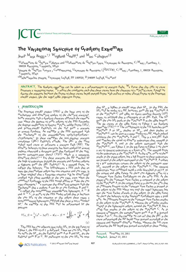
The Variational Structure of Gradient Extremals
Josep Maria Bofill,*,†,‡ Wolfgang Quapp,§ and Marc Caballero‡,∥
†Departament de Química Organica and ∥Departament de Química Física, Universitat de Barcelona, C/Martí i Franques, 1,08028 Barcelona, Catalunya, Spain‡Institut de Química Teorica i Computacional, Universitat de Barcelona (IQTCUB), C/Martí i Franques, 1, 08028 Barcelona,Catalunya, Spain
§Mathematisches Institut, Universitat Leipzig, PF 100920, D-04009 Leipzig, Germany
ABSTRACT: The gradient extremals can be taken as a representation of reaction paths. We prove that this type of curvepossesses a variational nature. We report the conditions such that these curves have the character of a minimal curve. Finally wediscuss the relations between the points of these curves being turning points with respect to other special points of the potentialenergy surface, like the valley-ridge inflection points.
1. INTRODUCTION
The potential energy surface (PES) is the basic tool of themechanistic and dynamical studies of the chemical reactivity.Some reactions with a diradical character approach the extremecase where the flatness of some regions of the PES precludesthe definite assignment of distinct minima, saddle points (SPs),and lowest-energy pathways on the way from a reactantto several products. An example is the PES associated withthe mechanism of the rearrangement vinylcyclopropane−cyclopentene.1 In these examples the non-intrinsic reactioncoordinate (IRC) pathways emerge. The IRC is the mostwidely used curve to represent a reaction path (RP). Thedynamic behavior of these reactions has been studied by severalauthors observing a deviation from that predicted by the well-known transition-state theory (TST) which is a statistical,dynamical theory.2−5 For these reactions the RP matched bythe bulk of trajectories joining the reactant and product regionsis different from the IRC pathway.6 As a starting point, weexplain this behavior. One hypothesizes a PES such that anutter flat intermediate region has one entrance and two exits. Itis quite unlikely that a particular entrance will be dynamicallycoupled with equal strength to the two exits, even when thesymmetry properties of the PES would appear to make the twoexits equivalent.2 We associate this dynamical situation with themechanism that a reagent A can go to two products B and C.We explain this nonsymmetric rearrangement bifurcation, A → Band A → C, in terms of the PES model saying that in betweenthe two SPs of the entrance to this region there exists anonsymmetrical bifurcation implying that there is not a monkeySP.7 An example of this PES may be represented by thefunction
= − − π − + + +⎜ ⎟
⎛
⎝⎜⎜⎛
⎝
⎞
⎠
⎞
⎠⎟⎟V x y x xy x y x y( , )
1
3( 3 ) ( )
1
40
7
4
3 24
4
(1)
This PES has two adjacent first-order SPs. In the left panel ofFigure 1, the PES of eq 1 is depicted. There are two SPs, whichwe name the SPab for the pathway from A to B and SPbc for thepathway from B to C. By inspection of the two SPs, we note
that SPab is higher in energy units than SPbc. In this PES, theSPs may be nodes of a RP, however, from the left minimum Ato the minimum C top right, no direct steepest descent (SD)exists, or anything that is equivalent to an IRC path. The SDfrom the two SPs leads to the minimum B at the right bottom.The fat curves in the right panel of Figure 1 are gradientextremals (GE).8−18 The combination of the GE branches fromminimum A to SPab, further to SPbc, and then further tominimum C can be seen as a static model of a RP, which indeedconnects the two minimums A and C. This is a non-IRC pathand matches the cloud of dynamic trajectories that, starting inthe minimum A, end in the region associated with theminimum C, see Figure 2. In the left panel of Figure 2 we showa set of classical trajectories at a given time. The starting pointof the trajectories is the minimum A. At this time, some of themreside in the initial region, but a big portion of these trajectoriesare located in the region associated to the minimum B. A subsetof a few trajectories crosses the region of the transition stateSPbc arriving to the region of the minimum C. The classicaltrajectories were computed using a code described in ref 19. Inthe central and right panels we show two different times of aGaussian wave packet propagation on the same PES. At theinitial time the Gaussian wave packet is centered in the regionof the minimum A. In the central panel it is shown the time thatan important portion of the Gaussian wave packet is located inthe region of the PES where not only the valley bifurcates butalso the wave packet spreads in this region. In the right panelwe show the behavior of this quantum propagation after a longtime. An important portion of the Gaussian wave packet residesin the region of the minimum A, whereas the reminder residesmainly in the bifurcation region, around the minimum B, but asmall part resides in the region of the minimum C. As inclassical simulation, the transformation from A to B is favoredbefore A to C. For this example we can say that the IRC is thecurve representing the RP being more favored according to theclassical and quantum dynamic models, whereas the GE curverepresents the RP being less favored according to these models.
Received: November 10, 2011Published: January 23, 2012
Article
pubs.acs.org/JCTC
© 2012 American Chemical Society 927 dx.doi.org/10.1021/ct200805d | J. Chem. Theory Comput. 2012, 8, 927−935

The quantum propagation was computed using the MCTDHprogram.20−22 From the classical dynamic theory, the RPmodel, which always is represented by a curve, can be envisagedas the curve that matches in the best way the average inposition of the cloud of trajectories after a long time. In thepresent case, both the IRC and the GE play this role, becauseboth match the average of the two different clouds oftrajectories after a long time.23 From a quantum point ofview this relation between quantum dynamics and RP model ismore difficult. However, in some cases we can say that thecurve representing a RP can be seen as the curve that matchesin the best way the maximum of the square of the wavefunction with respect to the position after a long time.24
Nevertheless, in the present study we are interested in thevariational properties of the GE curves. The GEs are curves thatusually run along valley floors or ridges of a PES. Morerigorously and specifically speaking, the GEs of a PES, V(q), aredefined as the curves, q(t), where t is the curve parameter,which cuts at each point a member of the isopotentialhypersurfaces of this PES, V(q(t)) = v(t), and the square of thegradient norm, ∇q
TV(q)∇qV(q) = g(q)Tg(q), is stationary ateach point of this curve in respect of the variations of q within
the member of isopotential hypersurfaces that is cut by thecurve at this point.11,16 Because one can use GEs as modelreaction pathways, we treat this kind of curves in this letter. Wenote that also another sort of curves, Newton trajectories(NT),25−29 is well adapted to the connection of adjacent SPs,compare refs 30 and 31 and references therein.As explained before in studies on dynamics of chemical
reactions, examples of nonstatistical dynamical behavior in largeorganic systems involve cases in which transient intermediatesoccupy plateau regions or at best shallow minimums on thePES.These regions are accessible by GEs, and due to this fact, a
GE can be seen as a representation of some average of arepresentative ensemble of classical trajectories.In principle it is plausible to believe that intermediates in
deeper minimums show some statistical behavior due to thehigher density of vibrational states at energies near their exitchannels. A rapid intramolecular vibrational energy redistri-bution should often be present. But examples of this kind suggestthat nonstatistical dynamics can persist even in these cases.The RP model is roughly defined as a curve in the coordinate
space, which connects two minimums by passing the SP, the
Figure 1. Left panel: PES associated to the mechanism of the reaction A → B + C. The mechanism for this reaction consists of two elementaryreactions, namely, A→ B and A→ C. Each product is associated with different minimums in the PES. Right panel: GE in the enlarged center of theleft panel. VRI: The valley from minimum B separates into two valleys over the SPs and a ridge between. The VRI point is crossed by the GE, whichconnects the two adjacent SPs.
Figure 2. Left panel: A representative set of exact classical trajectories on the PES given in eq 1. A static RP, which is represented by a curve, can beunderstood as the curve that matches the average position of the cloud of trajectories after a long time. The IRC can be seen as an approximation tothe average position of the set of trajectories that goes from the minimum A to B, whereas the GE curve is the approximation from A to theminimum C. Central panel: Quantum propagation of a Gaussian wave packet at the time that spreads into the bifurcation region of the PES.Notice that an important portion of the Gaussian wave packet resides in the region of the minimum A. Right panel: The propagation of the Gaussianwave packet at a latter time. Portions of the wave packet reside in the bifurcation region and the minimums as well. The portion of wave packet in theminimum B is bigger than that the minimum C.
Journal of Chemical Theory and Computation Article
dx.doi.org/10.1021/ct200805d | J. Chem. Theory Comput. 2012, 8, 927−935928

transition structure (TS) of a PES. If the RP curve is totallyconfined in a valley floor, then the RP takes the category of aminimum energy path (MEP). It is a secondary question, howa RP ascends to the SP and descends from it to a minimum.This looseness makes a variety of RP definitions possible, themost widely used being the IRC, the NT and the GE type ofcurves. A parametrization t of the RP curve q(t) = (q1(t), . . .,qN(t))
T is called reaction coordinate. In the last years the use ofthe variational theory of calculus of variations in the analysisand derivation of the different type of curves satisfying thefeatures of the RP model has been reviewed.31−46 Thevariational analysis of a RP curve representation provides, atleast from a mathematical point of view, the nature and thefeatures of the associated curves to this representation, like theextremal properties do, and what type of curves satisfy theminimum conditions. As noted before, the GE model has beenstudied in detail by the works of Ruedenberg and Jensen,17,18
however in this article we present a study based on the theoryof calculus of variations47 to give the grounds and features ofthis type of curve.In this article we analyze the variational nature of the GE
curves and their implications. Also the tangent of a GE curve isderived through a perturbation method widely used in quantummechanics. The characterization of a GE curve as a maximumor minimum is reported. The relation between special points ofthe GE curve in respect of special points of the PES isdiscussed. Finally some conclusions are given.
2. LAGRANGE−BOLZA VARIATIONAL PROBLEM AS ATHEORETICAL BASIS OF THE GE CURVES
2.1. The First-Order Variational Condition. We showhere that, in contrast to a remark in ref 44, the GE curves areextremal curves that belong to the problem of the theory ofcalculus of variations called Lagrangian or Bolza problem.48,49
Briefly, within the possible generalizations of the simplestproblems in the calculus of variations, one of the mostimportant is the well-known problem of Lagrange and itsgeneralizations, the so-called Bolza problem. In this type ofvariational problem, the extremal curve affording a stationaryvalue to the fundamental integral is required to satisfy certainsubsidiary conditions. The same requirements are also imposedon the curves of comparison being necessary to evaluate andanalyze the necessary and sufficient extremal conditions.The definition of a GE curve implies that as the curve evolves,
the hypersurface v changes as a function of t, the parameter thatcharacterizes the curve. In order to formulate the present problem,it is important to take into account that the arguments of thefunctional are subject to the boundary conditions and anadditional condition. These conditions refer to the entire courseof the arguments of the functional leading to an essentialmodification of the Euler differential equations. We are facing avariational problem with a finite subsidiary condition. The specificformulation consists in making the integral
∫ ∫= =
′ ′
I F t t tq q g g( ) ( , )d 1/2 d
t
t
t
tT
0 0 (2)
stationary in comparison to curves q(t) which satisfy in addition tothe boundary conditions, q(t0), q(t′), a subsidiary condition of theform
= − =G t V t v tq q( , ) ( ( )) ( ) 0 (3)
where as before g = ∇qV(q(t)). Geometrically speaking, we wantto determine a curve q(t) lying on the PES by the extremalrequirement. This problem can be formulated in a more compactform in the following way:
∫ ∫
∫
= = − λ
= − λ −
′ ′
′
I L t t F t t G t t
t V t v t t
q q q q q
g g q q
( ) ( , )d [ ( , ) ( ( )) ( , )]d
{1/2 ( ( ))[ ( ( )) ( )]}d
t
t
t
t
t
tT
0 0
0 (4)
where λ is the Lagrangian multiplier which depends on t throughq. The extremal curve satisfies the following set of equations ateach point
− − ∇ λ − λ =V vHg q q q g 0[ ( ) ] ( ) ( )q (5)
where we have dropped the dependence on t and H = ∇q gT is
the Hessian matrix at the point q of the PES. Equation 5 is theresulting Euler−Lagrange equation of the variational problem (eq 4).Substituting eq 3 into eq 5 we get
− λ =Hg q g 0( ) (6)
It means that the gradient is an eigenvector of the Hessian. It is the“coining” property of GEs. To eliminate the Lagrange multiplierλ(q) from eq 6, we first multiply it from the right by gT/gTg and itstransposed form from the left by g/gTg, subtracting and taking intoaccount that H = HT, we obtain
− = − =Hgg
g g
gg
g gH HP PH O
T
T
T
T(7)
where P is the projector onto the g subspace and O is the zeromatrix. This equation is necessary but not sufficient; it must becombined with the auxiliary condition that the eigenvector is normal
| | | | =− −g g g g( ) ( ) 1T1 1(8)
where |g| = (gTg)1/2. Multiplying this condition from the left byg |g|−1 and from the right by gT |g|−1, we get
= = =gg
g g
gg
g gPP P
gg
g g
T
T
T
T
T
T(9)
The condition 9 is called idempotency being characteristic of theprojectors like P introduced in eq 7. We emphasize that eqs 7 and 9are equivalent to the eq 6 and the normalization condition,(eq 8). Finally, from eq 9 we have,O = P − PP = (I − P) P, whereI is the unity matrix and (I − P) is the projector that projects tothe orthogonal subspace of the subspace spanned by the g vector. Ifwe multiply eq 7 from the left by (I − P) and from the right by g weobtain, using the last equality
− = − =⎛
⎝⎜⎜
⎞
⎠⎟⎟I P HPg I
gg
g gHg 0( )
T
T(10)
Equations 9 and 10 are equivalent to eq 6 and the normalizationcondition, (eq 8). Equation 6 plus the normalization condition(eq 8) or eqs 7 and 9 or eqs 10 and 9 are equivalent forms toprovide the necessary and sufficient conditions for the stationarity ofthe functional (eq 4). In ref 17, eq 10 was used as the starting pointto implicitly obtain the curve solution, q(t), the GE.
Journal of Chemical Theory and Computation Article
dx.doi.org/10.1021/ct200805d | J. Chem. Theory Comput. 2012, 8, 927−935929

2.2. Tangent Derivation of the Extremal Curve, GE,from an Application of Perturbation Theory. In thevariational problem (eq 4), the integrand does not involve thetangent argument, t = dq/dt. Thus, the set of Euler−Lagrangeequations reduces to the simple form given in eqs 6 and 8 ortheir equivalent form 7 and 9. Either of these two sets ofequations determines the GE curve q = q(t) implicitly. We notethat in this case the boundary values, q0 = q(t0) and qf = q(tf),cannot be prescribed arbitrarily if the problem should have asolution.47 On the contrary, one has to look for a solutionstarting at a q0 and take the value qf from there. The tangentvector, t, is necessary to integrate the curve but it does notappear in the expression. Here we use the perturbation theorydue to McWeeny which is widely used in quantum mechanics50
to implicitly derive the tangent of the GE from the eqs 7 and 9.First we assume that the current point, q = q(t), is located on aGE, so that the eqs 7 and 9 are satisfied.The basic idea is to start at a point located on a GE in the
absence of any first-order variation in q and to seek thenecessary first-order changes in the gradient to maintain the GEcondition when the perturbation in q is applied. In this mannerthe first-order variation in the gradient due to the first-orderperturbation in q is the tangent of the GE. With eq 7, theproblem of perturbation theory merely consists of restoring theGE condition when, due to a perturbation or variation in q,H → H + ΔH, and other quantities, change accordingly. Thisproblem is easily solved using the properties of projectionoperators.Let us assume that all quantities appearing in eqs 7 and 9 can
be expanded in powers of a perturbation parameter t, so that
= + − + −
+ = + − + − +
= =
t td
dtt t
d
dt
t t t t
H H H H
H H H
( ) ( )1
2
... ( ) ( ) ...
q q q q
0 0 02
2
2
0 0 0(1)
02
0(2)
0 0
(11a)
= + − + −
+ = + − + − +
= =
t td
dtt t
d
dt
t t t t
P P P P
P P P
( ) ( )1
2
... ( ) ( ) ...
q q q q
0 0 02
2
2
0 0 0(1)
02
0(2)
0 0
(11b)
where H0 and P0 are the unperturbed Hessian and projectormatrices evaluated at the point q0 = q(t0) belonging to theextremal curve. From the eqs 7, 11a, and 11b separating theorders, it follows readily that
+ − + =H P H P P H P H O( ) ( )0 0(1)
0(1)
0 0 0(1)
0(1)
0 (12)
will determine the first-order change in P0 with the auxiliaryequation
+ =P P P P P0 0(1)
0(1)
0 0(1)
(13)
which arises from eq 9. This auxiliary condition requires thatP0(1) be of the form
= = − + −=t
PP I P M P P M I P
d
d( ) ( )T
q q0(1)
0 0 0 0 0 0
0
(14)
where the matrix M0 is
= ==
− −⎛
⎝
⎜⎜
⎞
⎠
⎟⎟t
M Hq
g g g H t g g gd
d( ) ( )T T T T
q q0 0 0 0
10 0 0 0 0
10
0
(15)
where g0 and t0 are the gradient and the tangent vectorsevaluated at q0 = q(t0), respectively. The form of the M0 matrixresults from the application of the directional derivative, d/dt =[∇q ](dq/dt) = [∇q ]t, on the normalized gradient vector,being ∇q
T = (∂/∂q1, ..., ∂/∂qN). On substituting eq 14 in eq 12and multiplying from the left and right by (I − P0) and P0,respectively, we obtain
− − − −
+ − =
I P H I P M P I P M P H P
I P H P O
( ) ( ) ( )
( )
0 0 0 0 0 0 0 0 0 0
0 0(1)
0 (16)
where we have noted that H0P0 − P0H0 = O and that (I − P0)P0 = O. The eq 16 incorporates all quantities and completelydetermines the first-order change in P0
(1), which in turndetermines the tangent vector, t0, of the gradient extremal at q0.A solution is obtained most conveniently by multiplying
eq 16 from the right by g0 |g0|−1, then we have
− ⟨ ⟩ + − =⎛
⎝
⎜⎜
⎞
⎠
⎟⎟
⎡
⎣
⎢⎢
⎤
⎦
⎥⎥
Ig g
g gF g H
g H g
g gH t 0
T
T
T
T0 0
0 0
0 0 02 0 0 0
0 0
0 0(17)
where we have applied that (I − P0)H0P0 = O, since q0 is apoint of the GE. F0 is the third energy derivative tensor withrespect to q evaluated at q0. The ⟨F0g0⟩ symbolism is used toindicate a square matrix that is a contracted product of a three-index array with a vector yielding a two-index array; thus,
∑⟨ ⟩ ==
gF g F( )ij
k
N
ijk k0 01
00
(18)
where g0k is the k element of the g0 vector. The term ⟨F0g0⟩arises from the last term of the left-hand side part of eq 16, thatis
= = ⟨ ⟩ = ⟨ ⟩=
⎛
⎝
⎜⎜
⎞
⎠
⎟⎟
d
dtH g H g F t g F g t
q q0(1)
0 0 0 0 0 0 0 0
0 (19)
where the directional derivative and eq 18 have been used. Theeq 17 was derived for the first time by Sun and Rudenberg.17
We represent the projector (I − P0) = V0 V0T being V0 a
rectangular matrix of dimension N × (N−1) containing theN−1 eigenvectors of H0 orthonormal to g0 |g0|
−1 and thetangent vector as t0 = g0 |g0|
−1 eg0 + V0 e
0N − 1, where e
0N − 1 is a
vector of dimension N−1. Substituting this in eq 17 we obtainafter multiplying from the left by V0
T
− ⟨ ⟩| |
= ⟨ ⟩ + − −
⎡
⎣
⎢⎢
⎤
⎦
⎥⎥
eV F gg
gV F g H
g H g
g gH V eT
gT
T
T N0 0 00
0
00 0 0 0
2 0 0 0
0 0
0 0 10
(20)
Notice that V0T H0 V0 = DH0
N−1 = {h ij0 δij}i,j=1
N−1 , V0T H0 g0/
|g0|−1 = 0N−1 and V0
T V0 = IN−1 because we are in a point of aGE. The vector 0N−1 is the zero vector of dimension N−1, whileIN−1 is the unitary matrix of dimension (N−1) × (N−1).When the determinant of the square matrix of the right-hand side
Journal of Chemical Theory and Computation Article
dx.doi.org/10.1021/ct200805d | J. Chem. Theory Comput. 2012, 8, 927−935930

part of eq 20 is different from zero, then the vector e0N−1 isobtained as a function of eg
0, and the latter is evaluated by anormalization of the vector e0
T = (eg0, (e0N−1)
T). This completelydetermines t0 the tangent vector of the GE at q0.2.3. Special Points of GE Curves. We analyze the form of
the solutions of the eq 20. In case that the determinant of thesquare matrix appearing on the right-hand side part of eq 20 isequal zero, a careful analysis of this equation should be takeninto account to evaluate e0. For a deeper analysis of thissituation see refs 17 and 18. Such points where the gradientextremal has a det(V0
T[<F0g0> + H02 − λ0H0]V0) = 0 being λ0 =
g0TH0g0/(g0
T g0) can be either a turning point (TP), a pointwhere the curve touches the isopotential energy contourtangentially, or a bifurcation point (BP), a point where two GEscross. The structure of the tangent vector e0 is obtained in thesepoints by transforming the eq 20 in the set of coordinates thatdiagonalizes the square matrix appearing on the right-hand sidepart of this equation,
⟨ ⟩ + − = =⎡
⎣
⎢⎢
⎤
⎦
⎥⎥
V F g Hg H g
g gH V V C V U C UT
T
TT
DT
0 0 0 02 0 0 0
0 0
0 0 0 0 0 00
0
(21)
Where U0 is the unitary matrix of dimension (N−1) × (N−1)such that it diagonalizes the V0
TC0V0 matrix and C0D =
{c0ij, δij}i,j=1N−1, then eq 20 is transformed to
=eb C wg D00 0
0 (22)
being b0 = −U0TV0
T⟨F0g0⟩g0|g0|−1, and w0 = U0
Te0N−1, bothvectors of dimension N−1. As explained above, ifdet(V0
TC0V0) ≠ 0 then the tangent vector in the originalcoordinates is t0 = eg
0(g0 |g0|−1 + V0U0(C
0D)−1b0), where eg
0 iscomputed by a normalization of t0 vector. If det(V0
TC0V0) = 0,then at least one element of the diagonal matrix C0
D is equalzero. Let us assume that cii
0 = 0, then if the i element of the b0vector, bi
0, is different from zero, the solution of eq 22 plus thenormalization condition implies that eg
0 = 0 and w0T = (01, ...,
1i, ..., 0N− 1), and from this, the tangent takes the following forme0T = (e g
0, (eN − 10 )T) = (0, w0
T U0T) = (0, (ui
0)T), where ui0 is
the i column vector of the U0 matrix. The resulting normalizedtangent vector in the original coordinates is t0 = V0ui
0, where itdoes not have the component in the eigenvector pointing in thesame direction to the gradient vector, thus eg
0 = 0. Due to thisfact, at this point the GE does not cross the isopotential energycontour. It touches tangentially this isopotential contour. Thispoint is a TP for this GE, and we say that the curve ischaracteristic at this point.51,52 An example of two TPs is thePES depicted in Figure 1. The points at ∼(−0.25, −0.80) and∼(0.0, 1.0) are TPs of the central GE curve.In case that both cii
0 = 0 and bi0 = 0, then eq 22 plus the
normalization condition gives two solutions: one is that whichtouches the isopotential energy contour being the expression ofthe tangent the same as the one given above. The secondsolution is that which crosses the isopotential energy contour.In this case w0
T = eg0(c11
0 /b10, ..., 0i, ..., cN−1N−1
0 /bN−10 ) and
from this the tangent e0 takes the form e0T = (eg
0, (eN−10)T) =
eg0 (1, w0
TU0T), where e g
0 is computed by a normalization of e0vector. The resulting normalized tangent vector in the originalcoordinates takes the form t0 = e0g (g0|g0|
−1 + V0U0w0). The GEcurve with this tangent is a noncharacteristic curve at this point,it transverses the isopotential energy contour because eg
0 ≠ 0.Since in a point where both cii
0 = 0 and bi0 = 0, two GE curves
coincide at this point one with tangent t0 = V0ui0 and the other
with tangent t0 = e 0g (g0|g0|
−1 + V0U0w0), this point is calledbifurcation point (BP) for this type of GE curves. It isinteresting to notice that the structure of eq 20 is very close tothe basic equation to integrate Newton Trajectory curves asone can see by an inspection of eq (31) of ref 31, see also refs29 and 53. The basic differences between both equations lie inthat the vector of the left-hand side part of eq 20 depends onthe Hessian matrix rather than a contracted product of a three-index array with the gradient vector and that the square matrixof the right-hand side part is only a function of the Hessianmatrix.An example of a GE bifurcation is shown in Figure 3, on the
well-known Muller−Brown PES (mb-PES).54 At point ∼(0.06,
2.06) a bifurcation of the GE curve takes place. Note that thetwo eigenvalues of the Hessian matrix at this node
=−
−
⎛
⎝⎜
⎞
⎠⎟H(0.06 2.06)
1902.96 389.644
389.644 1902.96
are totally different: they are 1513.31 and 2292.6. By the way,the GE curve starting orthogonally to the minimum valleymeets itself at the BP. There is also its TP at the slope of thebowl.Now we show by an example that a degeneracy of eq 6
involving the eigenvector that points in the same direction tothe gradient vector does not affect the behavior of the actualGE curve. Let us assume that on a point at the GE curve theHessian is degenerated, but det(H) ≠ 0, and one of thedegenerated eigenvectors coincides with the gradient directionat this point. Nevertheless, the derivation of the tangent of thecurve due to Ruedenberg’s formula, eq 17, is true and the GEcurve behaves ‘normally’. In Figure 4 we again demonstrate thiswith the mb-PES. We again show the GE curves of Figure 3 andthe level lines of two eigenvalues: The value of each of them isequal to 313.1 units. The two systems cross exactly at the GEcurve near the deep minimum. There the GE curve does notshow any anomaly.Finally, we say that the perturbational method due to
McWeeny50 has been used until now to derive the well-knowntangent vector that characterizes the GE curve. Using the samemethod one can evaluate the first-order gradient correctionthrough the GE curve, g(q(t)). For this task, first we insert
Figure 3. GE curves (fat dashes) on the mb-PES.
Journal of Chemical Theory and Computation Article
dx.doi.org/10.1021/ct200805d | J. Chem. Theory Comput. 2012, 8, 927−935931
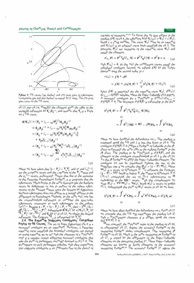
eq 15 into eq 16, multiply the equation from the right of theresulting expression by g0 |g0|
−1, and assume that q0 is a pointon a GE curve,
∑
≈ + − | |
= | | + − | |
= + − | |
+ | |
= + − | |
= + − | |
−
− −
−
−−
−−
−
=
−
−−
t t t
t t
t t e
t t
t t h e
g q P P g g
g g V V H t g
g V V H g g
V e g
g V H e g
g v g
( ( )) ( ( ) )
( )
( ( ) (
))
( ( ) )
( ( ) ( ) )
T
Tg
N
D NN
i
N
i ii N i
0 0 0(1)
0 01
0 01
0 0 0 0 0 01
0 0 0 0 0 0 01 0
0 10
01
0 0 0 01
10
01
0 01
10 0
10
01
(23)
where we have taken that (I − P0) = V0V0T and vi
0 and (e0N−1)i
are the i column vector and the i element of the V0 matrix andthe e0
N−1 vector, respectively. Notice that due to the structureof this particular perturbation problem, it is irrelevant that theeigenvector which points in the same direction like the gradientvector be degenerate or not in respect of the others eigen-vectors of the Hessian matrix, since the division by differencesbetween eigenvalues does not appear as it usually appears in theapplication of perturbation methods. In the same way, one hasthe corresponding expression to compute the first-ordereigenvector correction to each eigenvector of the subset,{vi
0}i=1N−1. Because I = P0 + (I − P0) = P0 + Q 0 then − dQ 0/dt =
dP0/dt = −Q0(1) = P0
(1). Substituting g(q(t)) by vi(q(t)), P0 byQ 0, P 0
(1) by −Q 0(1) and g0 by vi
0 in eq 23, we obtain the desiredexpression. The projector Q 0 is represented by V0V0
T .2.4. The Extremal Sufficient Conditions. Conjugate
Points of GE Curves. The set of Euler differential eqs 6 is anecessary condition for an extremum. However, a particularextremal curve satisfying the boundary conditions can furnishan actual extremal, let us say with the character of a minimum,only if it satisfies certain additional necessary conditions thattake the form of inequalities, normally denoted as δ2I ≥ 0. Theformulation of such inequalities together with their refinementinto sufficient conditions is an important part of the theory of
calculus of variations.47,55 To prove this we first replace in theintegral I(q) of eq 4, the argument q by qC(t,ε) = q(t) + ε p(t),being ε a small number. The curve q(t) must be an extremaland qC(t,ε) is an arbitrary curve both satisfying the eq 3. Thefunctions p(t) are variations of the extremal curve q(t) andsatisfy the equation:
= ∇ = ∇ = =P t G t Vp p q p q p g( , ) ( , ) ( ) 0T T Tq q (24)
with p(t0) = 0. In this way the comparison curves satisfy thesubsidiary condition. Second, we expand I(q) by the Taylortheorem until the second order in ε
ε = + ε
= + εδ +ε
δ + ε
H I
I I I O
q p
q q p q p
( ) ( )
( ) ( , )2
( , ) ( )2
2 2(25)
Since I(q) is stationary for the extremal curve q(t), dH(ε)/dε |ε=0 = δI(q,p) vanishes, where the Euler−Lagrange eq 6 follows.A necessary condition for a minimum is d2H(ε)/d2ε|ε=0 =δ2I(q,p) ≥ 0. The derivative δ2I(q,p) is expressible in the form
∫
∫ ∫
δ = ∇ ∇
= ⟨ ⟩ + − λ =
′
′ ′
I L t t
t t
q p p q p
p Fg H H p p Cp
( , ) [ ( , )] d
[ ] d d
t
tT T
t
tT
t
tT
q q2
2
0
0 0
(26)
where we have dropped the dependence on t. This integral isevaluated along the GE and λ is just that given in eq 6. Thecondition δ2I(q,p) ≥ 0 implies a problem of Lagrange in the tp-space of precisely the same type as the original problem in thetq space. The integral to be minimized is δ2I(q,p), and theequation of the condition corresponding to eq 3 is the eq 24.To this tp problem we apply the Euler−Lagrange equation. Thecondition 24 can be introduced without the use of themultiplier rule if we consider that p(t) = (I − P) m(t), wherem(t) is a vector of dimension N. We represent the projector(I − P) = VVT being as before V, the matrix of dimension N ×
(N−1) containing the set of N−1 eigenvectors of Horthogonal to the g|g|−1 vector. With this consideration wewrite p(t) = VVTm(t) = Vn(t), being n(t) a vector of lengthN−1. Substituting this form of p(t) vector in eq 26 we have,
∫ ∫δ = = = δ
′ ′
I t t Iq p p Cp n V CVn q n( , ) d d ( , )
t
tT
t
tT T2 2
0 0
(27)
where we have again dropped the dependence on t. From eq 27we conclude that the GE will extremalize the integral (eq 4)with a minimization character if it applies along the curvedet(VTCV) ≥ 0.More concisely, the minimum value of the integral of eq 26,
or equivalently eq 27, defines the accessory problem of thevariational problem under consideration. This variational tpproblem of eq 26, which is the same variational tn problem ofeq 27, is solved by the application of the Euler−Lagrangeequations on the functional integral 27. These Euler−Lagrangeequations are known as Jacobi equations of the accessoryvariational problem.56 The accessory problem 27 affects the
Figure 4. GE curves (fat dashes) and two level lines of eigenvalues(continuous line and thin dashes) at exactly 313.1 units. The two levellines cross on the GE curve.
Journal of Chemical Theory and Computation Article
dx.doi.org/10.1021/ct200805d | J. Chem. Theory Comput. 2012, 8, 927−935932
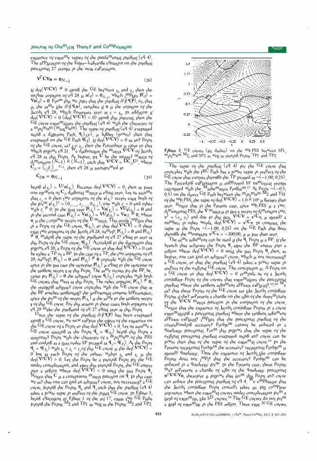
existence of extreme values of the fundamental integral (eq 4).The application of the Euler−Lagrange equation on the integralfunctional 27 results in the next expression:
= −V CVn 0TN 1 (28)
If det(VTCV) ≠ 0 along the GE between t0 and t′, then theunique solution of eq 28 is n(t) = 0N−1, which implies p(t) =Vn(t) = 0. From this we infer that the integral δ2I(q,p), or, thatis, the same like δ2I(q,n), vanishes if n is the solution of theJacobi eq 28, which possesses zero at t = t0. In addition ifdet(VTCV) > 0 (det(VTCV) < 0) along this interval, then theGE curve extremalizes the integral (eq 4) with the character ofa minimum (maximum). The value of integral (eq 4) evaluatedusing a different path, qC(t,ε), is higher (lower) than thatevaluated on the GE path q(t). If det(VTCV) = 0 at any pointof the GE curve, say t = t1, then the procedure is close to thatwhich follows eq 21. We diagonalize the matrix VTCV of Jacobieq 28 at this point. As before, let U be the unitary matrix ofdimension (N−1) × (N−1), such that VTCV = UCDU
T, whereCD = {cijδij}i,j=1
N−1, then eq 28 is transformed to
= −C z 0D N 1 (29)
being z(t1) = UTn(t1). Because det(VTCV) = 0, then at leastone element of CD diagonal matrix is equal zero. Let us assumethat cii = 0 then two solutions of the z(t1) vector exist both ofthe form z(t1)
T = (01, ..., zi, ..., 0N−1), one with zi = 0 and otherwith zi ≠ 0. In the first case p(t1) = Vn(t1) = VUz(t1) = 0 andin the second case p(t1) = Vn(t1) = VUz(t1) = Vuizi ≠ 0, whereui is the i column vector of the U matrix. This result implies thatin a point of the GE curve, q(t1), so that det(VTCV) = 0 thereexist two solutions of the Jacobi eq 28, namely, p(t1) = 0 and p(t1)≠ 0, making the value of the integrand of eq 27 equal to zero atthis point of the GE curve, q(t1). According to the discussion thatfollows eq 20, a point of the GE curve so that det(VTCV) = 0 canbe either a TP or a BP. In the case of a TP, the two solutions of eq29, namely, p(t1) = 0 and p(t1) ≠ 0 coincide with the GE curvesince in the last case the structure p(t1) is equal to the structure ofthe tangent vector t at this point. The same occurs for the BP, be-cause for p(t1) = 0 the arbitrary curve qC(t1) coincides with bothGE curves that meet at this point. The other solution, p(t1) ≠ 0,the resulting arbitrary curve coincides with the GE curve that atthe BP touches tangentially the isopotential contour hypersurface,since the form of the vector p(t1) is the same to the tangent vectort of this GE curve. For this reason in these cases both solutions ofeq 29 make the integrand of eq 27 equal zero at this point.Once the value of the integral δ2I(q,p) has been evaluated
along a GE curve, we now explore the effect of the existence onthe GE curve of a point so that det(VTCV) = 0. Let us assume aGE curve starting at the point q0 = q(t0) being this point astationary point with the character of a minimum of the PESand ending at a first-order SP located at qf = q(tf). At the pointq1 = q(t1) with t0 < t1 < tf of this GE curve is the det(VTCV) =0 but at each point of the subarc within t0 and t1 is thedet(VTCV) > 0. Let the point be a turning point for the GEunder consideration, and after this turning point, the GE entersinto a region where det(VTCV) < 0 until the last point qf.Notice that C is a continuous matrix function on q. In this casewe say that one can find an arbitrary curve, not necessarily a GEcurve, joining the points q0 and qf such that the integral (eq 4)takes a lower value in respect of the initial GE curve. In Figure 5,being equivalent to Figure 1 of the ref 17, exists two GE pathsjoining the points M2 and TP1 as well as the points M2 and TP2.
The value of the integral (eq 4) for the GE curve thatcoincides with the IRC path has a lower value in respect of theGE curve that evolves through the TP located at ∼(−1.00, 0.25).The preceding explanation is supported by numerical resultscalculated with the Mathematica program.57 At point ∼(−0.5,0.5) on the direct GE path between the minimum M2 and TS1of the mb-PES, the value of det(VTCV) = 1.0 × 10⁶ is greater thanzero. Notice that in the present case, since mb-PES is a two-dimensional PES, the V matrix is in fact a vector of dimension two,vT = (vx, vy) and due to this fact, VTCV = vTCv, is already anumber; in other words, det(VTCV) = vTCv. In contrast, thevalue at the point ∼(−1.00, 0.25) on the GE path that goesthrough the mountains vTCv = −200.00, it is less than zero.The same argument can be used if the q1 point is a BP. If the
branch that achieves the point qf after the BP enters into aregion where det(VTCV) < 0 until the last point qf then, asbefore, one can find an arbitrary curve, which is not necessarilya GE curve, so that the integral (eq 4) takes a lower value inrespect of the original GE curve. The conclusion is: A point ona GE curve so that det(VTCV) = 0 reminds us of a Jacobiconjugate point of the curves that extremalizes the functionalintegral where the tangent argument appears explicitly.55,56 Wesay that these points of the GE curve are like Jacobi conjugatepoints if they represent a change on the sign of the determinantof the VTCV matrix function in the evolution of the curve.Notice that the existence of Jacobi conjugate points in a curveextremalizing a functional integral where the tangent argumentappears explicitly implies that the functional integral of thecorresponding accessory problem cannot be reduced to aquadratic functional. From this follows that the value of theoriginal functional integral evaluated using any curve can belower than that of the value of the extremal curve.55 In thepresent variational problem the accessory variational problem isalready quadratic. Thus the existence of Jacobi-like conjugatepoints does not imply that the accessory problem can bereduced in a quadratic form. In the present case, these pointsmay represent a change of sign of the quadratic functionalnTVTCVn, therefore it follows that from this point any curvecan reduce the functional integral of eq 4. We emphasize thatthe Jacobi conjugate point concept takes its full completerelevance when the extremal curves under consideration form afield of extremals, like SD curves.39 The GE curves do not forma field of extremals in the PES region. There exist N GE curves
Figure 5. GE curves (fat dashes) on the mb-PES between SP1,minimum M2, and SP2 as well as turning points TP1 and TP2.
Journal of Chemical Theory and Computation Article
dx.doi.org/10.1021/ct200805d | J. Chem. Theory Comput. 2012, 8, 927−935933

only if the dimension of the PES is N. Nevertheless, we say thatTP and BP points of a GE arc curve in some aspects resemble theoriginal Jacobi conjugate point concept, and due to this fact, wesay that these points can be seen as Jacobi-like conjugate points.
3. RELATION BETWEEN TPs OF A GE CURVE ANDVALLEY-RIDGE INFLECTION POINTS
Regarding Figure 1, a valley-ridge inflection point (VRI)emerges in the GE subarc that goes from the TP located at thepoint ∼(−0.2, −0.6) and to the TP located at the point ∼(0.0, 1.0).The VRI point is related to the existence of a bifurcation in the PES.The VRI is a feature of the PES and does not always have relationswith the nature of the curve.58 In Figure 4 of the mb-PES, looking atthe GE subarc being orthogonally to the GE RP at the minimumM2, which goes from the TP1 located at the point∼(−1.00, 0.25) tothe TP2 located at the point ∼(0.6, 0.6), a point of this subarc is theminimum M2. This GE subarc is orthogonal to the GE RP at thestationary point, M2. As before, a stationary point is a feature ofthe PES and does not always have relations to the nature of thecurve going through it. However the most important is a possiblerelation between TPs of a GE and VRIs of the PES. In Figure 5 ofref 59 is shown the TPs of the different GEs and the VRI points ofthe mb-PES. With this observation, we enunciate the nextproposition.A GE touches at its TP, q(tTP), a isopotential hypersurface of
the full PES. At other GE points, it crosses a family ofisopotential hypersurfaces transversally. We may assume that atq(tTP) and the next points q(t) of the GE, with tTP < t, thefamily of isopotential hypersurfaces is pseudoconvex with thepseudoconvexity index:60
μ = >g Ag
g g0 (or vice versa)
T
T(30)
If along the GE the index μ changes the sign then there is a VRIpoint. In eq 30 the A matrix is the adjoint matrix of the Hessianmatrix H, and it satisfies the relation, AH = I det(H).The proof of the proposition is the following: At the transition
point of the GE through the contour valley-ridge, we have to finda zero eigenvector of the Hessian matrix lying in the tangentialplane of the corresponding isopotential hypersurface. Because thispoint belongs to a GE, the gradient is an eigenvector of theHessian matrix, and due to this fact, the gradient vector isorthogonal to the eigenvector with null eigenvalue. This is nothingmore that the definition of a VRI point.60 Notice that it is notnecessary that a TP point of the GE curve exists before the GEtransverses a contour valley-ridge inflection. In Figure 5 of ref 59exists an isolated VRI point on a GE curve, but no TP of this GEexists near to this VRI point. On the other hand, there can be twoconsecutive TPs of a GE without a VRI point in between, seeagain Figure 5 of ref 59.Finally we remark that if a GE having a VRI point in a subarc,
then it does not imply that in this subarc det(VTCV) ≥ 0 holds,or vice versa. In other words, the VRI point does not affect theextremal character of the subarc. Let us assume a GE subarcwithout TP lifting a valley region with det(VTCV)) ≥ 0 andentering in a ridge region through a VRI point, where in thisnew region the GE has det(VTCV)) ≥ 0. This result is a directconsequence of the discussion of Section2.4.
4. DISCUSSION, SUMMARY, AND CONCLUSION
The GE curve can be used to determine the TS and intermediatesof any reaction mechanism starting at the reactant minimum.
Examples are demonstrated for methyleneimine (H2CNH)computed using a CASSCF calculation,13 the electrocyclic reactionof cyclobutene to butadiene,9 or the formation of amino-acetonitrile.61 As reported in the Introduction Section, the GEpath is also a type of curve that can be used as a representation ofa RP in the cases that fail the IRC as a representation. Due to theimportance of this type of path, we have proved the variationalnature of the GE path. GEs are curves where the norm of thegradient has a local extremum on isopotential hypersurfaces of thePES, V(q(t)) = v(t). An example is discussed in ref 53, where theIRC is going down across a ridge, but the GE represents the MEPwhich is parallel nearby. The PES of that example is a modifiedPES of an alanine dipeptide rearrangement.62 The GE paths areextremal curves of a variational problem that is formulated inexpression (eq 4). The tangent of this type of curves has beenderived using the perturbation theory due to McWeeny that iswidely used in quantum mechanics. In addition their extremalsufficient conditions are studied and reported being summarized asfollows. If the curve starts at a minimum of the PES withdet(VTCV) > 0, with eq 27, and ends at a first-order stationarypoint, the extremal curve achieves its condition of a minimal curve.However, if this curve has a TP or a BP, then from this point tothe end point may be det(VTCV) < 0, and the GE curve looses itsminimum character, see Figure 1. If det(VTCV) < 0 from the TPto the end point, then other curves exist. Not necessarily a GEcurve joins the initial and final point so that the integral (eq 4)takes a lower value. The TP and the BP of a GE curve can be seenas a Jacobi conjugate point of this type of curves. Nevertheless, thisequivalence should be taken carefully since the GE curves do notform a field of curves covering the PES region as occurs with theSD curves or with NTs. In the later cases the concept of Jacobiconjugate points takes its important relevance. The missing “field”
property may be an advantage of the GE calculation. In ref 30 wasfound a VRI point of the ring closure of the allyl radical, howeverthat point is located after a small ring-opening. The search withNT failed because it was done in the false direction. But a searchof the minimal GE along the minimum valley of the allyl radicalfound that point. The VRI points are important on PESs wherethe RP bifurcates.58 The relation between the VRI points and theGE curve is also analyzed. VRIs are the type of points related tothe curve which leaves a valley region and enters into a ridgeregion of the PES, or vice versa. The behavior of the GE path canbe used as a way to take information on the topology of the PESregion where the reaction mechanism takes place.63
■ AUTHOR INFORMATION
Corresponding Author*E-mail: [email protected]. Telephone: 34 93 402 11 96.
NotesThe authors declare no competing financial interest.
■ ACKNOWLEDGMENTS
Financial support from the Spanish Ministerio de Ciencia eInnovacion, DGI project CTQ2011-22505 and, in part fromthe Generalitat de Catalunya projects 2009SGR-1472 are fullyacknowledged. M.C. gratefully thanks the Ministerio de Cienciae Innovacion for a predoctoral fellowship.
■ REFERENCES
(1) Doubleday, C. J. Phys. Chem. A 2001, 105, 6333.(2) Carpenter, B. K. Angew. Chem., Int. Ed. 1998, 37, 3340.(3) Doubleday, C.; Li, G.; Hase, W. L. Phys. Chem. Chem. Phys. 2002,4, 304.
Journal of Chemical Theory and Computation Article
dx.doi.org/10.1021/ct200805d | J. Chem. Theory Comput. 2012, 8, 927−935934

(4) Carpenter, B. K. J. Phys. Org. Chem. 2003, 16, 858.(5) Doubleday, C.; Suhrada, C. P.; Houk, K. N. J. Am. Chem. Soc.2006, 128, 90.(6) Ammal, S. C.; Yamataka, H.; Aida, M.; Dupuis, M. Science 2003,299, 1555.(7) Valtazanos, P.; Ruedenberg, K. Theor. Chim. Acta 1986, 69, 281.(8) Pancir, J. Collect. Czech. Chem. Commun. 1975, 40, 1112.(9) Basilevsky, M. V.; Shamov, A. G. Chem. Phys. 1981, 60, 347.(10) Rowe, D. J.; Ryman, A. J. Math. Phys. 1982, 23, 732.(11) Basilevsky, M. V. Chem. Phys. 1982, 67, 337.(12) Hoffman, D. K.; Nord, R. S.; Ruedenberg, K. Theor. Chim. Acta1986, 69, 265.(13) Jørgensen, P.; Jensen, H. J. Aa.; Helgaker, T. Theor. Chim. Acta1988, 73, 55.(14) Quapp, W. Theor. Chim. Acta 1989, 75, 447.(15) Schlegel, H. B. Theor. Chim. Acta 1991, 83, 15.(16) Heidrich, D.; Kliesch, W.; Quapp, W. Properties of ChemicallyInteresting Potential Energy Surfaces, Lecture Notes in Chemistry;Springer-Verlag: Berlin, Germany, 1991; Vol. 56, Section 3.(17) Sun, J.-Q.; Ruedenberg, K. J. Chem. Phys. 1993, 98, 9707.(18) Bondensgard, K.; Jensen, F. J. Chem. Phys. 1996, 104, 8025.(19) Press, W. H.; Flannery, B. P.; Teukolsky, S. A.; Vetterling, W. T.Numerical Recipes in Fortran 77: The Art of Scientific Computing;Cambridge University Press: Cambridge, U.K., 2003.(20) Worth, G. A.; Beck, M. H.; Jackle, A.; Meyer, H.-D. TheMCTDH Package, version 8.2; University of Heidelberg: Heidelberg,Germany, 2000.(21) Meyer, H.-D.; Manthe, U.; Cederbaum, L. S. Chem. Phys. Lett.1990, 165, 73.(22) Beck, M. H.; Jackle, A.; Worth, G. A.; Meyer, H.-D. Phys. Rep.2000, 324:1, 1.(23) Gonzalez, J.; Gimenez, X.; Bofill, J. M. Phys. Chem. Chem. Phys.2002, 4, 2921.(24) Gonzalez, J.; Gimenez, X.; Bofill, J. M. J. Chem. Phys. 2009, 131,054108.(25) Quapp, W.; Hirsch, M.; Imig, O.; Heidrich, D. J. Comput. Chem.1998, 19, 1087.(26) Quapp, W.; Hirsch, M.; Heidrich, D. Theor. Chem. Acc. 1998,100, 285.(27) Anglada, J. M.; Besalu, E.; Bofill, J. M.; Crehuet, R. J. Comput.Chem. 2001, 22, 387.(28) Bofill, J. M.; Anglada, J. M. Theor. Chem. Acc. 2001, 105, 463.(29) Crehuet, R.; Bofill, J. M.; Anglada, J. M. Theor. Chem. Acc. 2002,107, 130.(30) Quapp, W.; Bofill, J. M.; Aguilar-Mogas, A. Theor. Chem. Acc.2011, 129, 83.(31) Bofill, J. M.; Quapp, W. J. Chem. Phys. 2011, 134, 074101.(32) Tachibana, A.; Fukui, K. Theor. Chim. Acta 1978, 49, 321.(33) Tachibana, A.; Fukui, K. Theor. Chim. Acta 1979, 51, 189.(34) Tachibana, A.; Fukui, K. Theor. Chim. Acta 1979, 51, 275.(35) Tachibana, A.; Fukui, K. Theor. Chim. Acta 1980, 57, 81.(36) Fukui, K. Int. J. Quantum Chem., Quantum Chem. Symp. 1981,15, 633.(37) Olender, R.; Elber, R. J. Mol. Struc. (THEOCHEM) 1997, 63,398.(38) Stacho, L. L.; Domotor, G.; Ban, M. I. J. Math. Chem. 2000, 28,241.(39) Crehuet, R.; Bofill, J. M. J. Chem. Phys. 2005, 122, 234105.(40) Aguilar-Mogas, A.; Crehuet, R.; Gimenez, X.; Bofill, J. M. Mol.Phys. 2007, 105, 2475.(41) Aguilar-Mogas, A.; Gimenez, X.; Bofill, J. M. J. Chem. Phys.2008, 128, 104102.(42) Vanden-Eijnden, E.; Heymann, M. J. Chem. Phys. 2008, 128,061103.(43) Heymann, M.; Vanden-Eijnden, E. Comm. Pure Appl. Math.2008, 61, 1052.(44) Quapp, W. Theor. Chem. Acc. 2008, 121, 227.(45) Bofill, J. M. J. Chem. Phys. 2009, 130, 176102.
(46) Aguilar-Mogas, A.; Gimenez, X.; Bofill, J. M. J. Comput. Chem.2010, 31, 2510.(47) Courant, R.; Hilbert, D. Methods of Mathematical Physics; Wiley:New York, 1953.(48) Caratheodory, C. Variationsrechnung und Partielle Differ-entialgleichungen Erster Ordnung; Teubner: Leipzig, Germany, 1935.(49) Bliss, G. A. Lectures on the Calculus of Variations; The Universityof Chicago Press: Chicago IL, 1946.(50) McWeeny, R. Phys. Rev. 1961, 126, 1028.(51) Petrovsky, I. G. Lectures on Partial Differential Equations; DoverPublications: New York, 1991.(52) John, F. Partial Differential Equations; Springer: Heidelberg,Germany, 1974.(53) Hirsch, M.; Quapp, W. Chem. Phys. Lett. 2004, 395, 150.(54) Muller, K.; Brown, L. D. Theor. Chim. Acta 1979, 53, 75.(55) Gelfand, I. M.; Fomin, S. V. Calculus of Variations; DoverPublications: New York, 2000.(56) Rund, H. The Hamilton-Jacobi Theory in the Calculus ofVariations; Van Nostrand: London, U.K., 1966.(57) Wolfram, S. Mathematica; Addison-Wesley: New York, 1988.(58) Quapp, W. J. Mol. Struct. (THEOCHEM) 2004, 695−696, 95.(59) Quapp, W.; Hirsch, M.; Heidrich, D. Theor. Chem. Acc. 2004,112, 40.(60) Hirsch, M.; Quapp, W. J. Math. Chem. 2004, 36, 307.(61) Koch, D. M.; Toubin, C.; Peslherbe, G. H.; Hynes, J. T. J. Phys.Chem. C 2008, 112, 2972.(62) Neria, E.; Fischer, S.; Karplus, M. J. Chem. Phys. 1996, 105,1902.(63) Lucas, J. M.; Andres, J.; de Sogas, J.; Albertí, M.; Bofill, J. M.;Bassi, D.; Ascenzi, D.; Tosi, P.; Aguilar, A. J. Chem. Phys. 2009, 131,024306.
Journal of Chemical Theory and Computation Article
dx.doi.org/10.1021/ct200805d | J. Chem. Theory Comput. 2012, 8, 927−935935
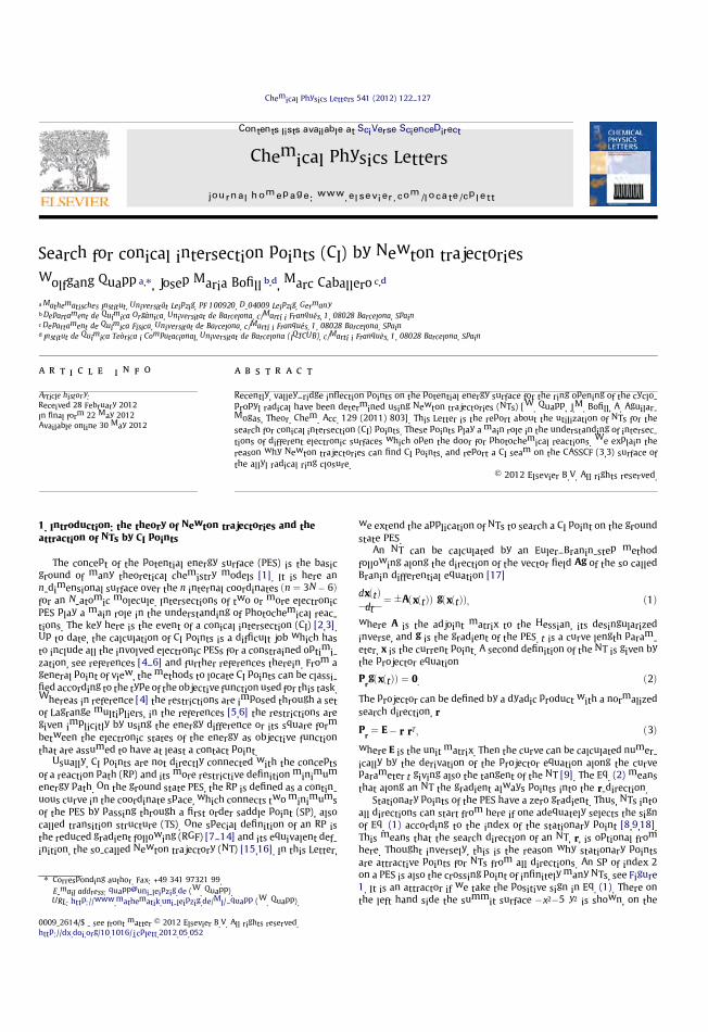
Search for conical intersection points (CI) by Newton trajectories
Wolfgang Quapp a,⇑, Josep Maria Bofill b,d, Marc Caballero c,d
aMathematisches Institut, Universität Leipzig, PF 100920, D-04009 Leipzig, GermanybDepartament de Química Orgànica, Universitat de Barcelona, c/Martí i Franqués, 1, 08028 Barcelona, SpaincDepartament de Química Física, Universitat de Barcelona, c/Martí i Franqués, 1, 08028 Barcelona, Spaind Institut de Química Teòrica i Computacional, Universitat de Barcelona (IQTCUB), c/Martí i Franquès, 1, 08028 Barcelona, Spain
a r t i c l e i n f o
Article history:
Received 28 February 2012In final form 22 May 2012Available online 30 May 2012
a b s t r a c t
Recently, valley–ridge inflection points on the potential energy surface for the ring opening of the cyclo-propyl radical have been determined using Newton trajectories (NTs) [W. Quapp, J.M. Bofill, A. Aguilar-Mogas, Theor. Chem. Acc. 129 (2011) 803]. This Letter is the report about the utilization of NTs for thesearch for conical intersection (CI) points. These points play a main role in the understanding of intersec-tions of different electronic surfaces which open the door for photochemical reactions. We explain thereason why Newton trajectories can find CI points, and report a CI seam on the CASSCF (3,3) surface ofthe allyl radical ring closure.
� 2012 Elsevier B.V. All rights reserved.
1. Introduction: the theory of Newton trajectories and the
attraction of NTs by CI points
The concept of the potential energy surface (PES) is the basicground of many theoretical chemistry models [1]. It is here ann-dimensional surface over the n internal coordinates ðn ¼ 3N À 6Þfor an N-atomic molecule. Intersections of two or more electronicPES play a main role in the understanding of photochemical reac-tions. The key here is the event of a conical intersection (CI) [2,3].Up to date, the calculation of CI points is a difficult job which hasto include all the involved electronic PESs for a constrained optimi-zation, see references [4–6] and further references therein. From ageneral point of view, the methods to locate CI points can be classi-fied according to the type of the objective function used for this task.Whereas in reference [4] the restrictions are imposed through a setof Lagrange multipliers, in the references [5,6] the restrictions aregiven implicitly by using the energy difference or its square formbetween the electronic states of the energy as objective functionthat are assumed to have at least a contact point.
Usually, CI points are not directly connected with the conceptsof a reaction path (RP) and its more restrictive definition minimumenergy path. On the ground state PES, the RP is defined as a contin-uous curve in the coordinate space, which connects two minimumsof the PES by passing through a first order saddle point (SP), alsocalled transition structure (TS). One special definition of an RP isthe reduced gradient following (RGF) [7–14] and its equivalent def-inition, the so-called Newton trajectory (NT) [15,16]. In this Letter,
we extend the application of NTs to search a CI point on the groundstate PES.
An NT can be calculated by an Euler–Branin-step methodfollowing along the direction of the vector field Ag of the so calledBranin differential equation [17]
dxðtÞdt
¼ ÆAðxðtÞÞ gðxðtÞÞ; ð1Þ
where A is the adjoint matrix to the Hessian, its desingularizedinverse, and g is the gradient of the PES. t is a curve length param-eter, x is the current point. A second definition of the NT is given bythe projector equation
PrgðxðtÞÞ ¼ 0: ð2Þ
The projector can be defined by a dyadic product with a normalizedsearch direction, r
Pr ¼ EÀ r rT ; ð3Þ
where E is the unit matrix. Then the curve can be calculated numer-ically by the derivation of the projector equation along the curveparameter t giving also the tangent of the NT [9]. The Eq. (2) meansthat along an NT the gradient always points into the r-direction.
Stationary points of the PES have a zero gradient. Thus, NTs intoall directions can start from here if one adequately selects the signof Eq. (1) according to the index of the stationary point [8,9,18].This means that the search direction of an NT, r, is optional fromhere. Thought inversely, this is the reason why stationary pointsare attractive points for NTs from all directions. An SP of index 2on a PES is also the crossing point of infinitely many NTs, see Figure1. It is an attractor if we take the positive sign in Eq. (1). There onthe left hand side the summit surface Àx2À5 y2 is shown, on the
0009-2614/$ - see front matter � 2012 Elsevier B.V. All rights reserved.http://dx.doi.org/10.1016/j.cplett.2012.05.052
⇑ Corresponding author. Fax: +49 341 97321 99.
E-mail address: [email protected] (W. Quapp).URL: http://www.mathematik.uni-leipzig.de/MI/~quapp (W. Quapp).
Chemical Physics Letters 541 (2012) 122–127
Contents lists available at SciVerse ScienceDirect
Chemical Physics Letters
journal homepage: www.elsevier .com/locate /cplet t

upper left hand panel, and on the lower line the field Ag is shown.The summit is at the point (0,0); it is an SP of index 2. Starting anNT uphill anywhere around the summit it will find the summit it-self. Analogously, a funnel surface of a typical peaked ðnÀ 2Þ CIevent [2,3] is shown on the right hand side of Figure 1. It is the sur-faceÀsqrtðx2 þ 5y2Þ. Here, an analogous vector field Ag emerges. Atthis point it is important to emphasize that both types of problems,finding an SP of index two, a summit, or a peaked ðnÀ 2Þ conicalintersection point, are quite close, both conceptually and computa-tionally. This is a hint that the NT method too finds CI points aswell as summits. However, there are differences to the summitcase:
(i) The two components of the gradient in the branching sub-space do not go to zero around the peacked ðnÀ 2Þ-CI point,but hold any slope, and their direction is indefinite at the CIpoint. In Figure 1 right panel the gradient is
1ffiffiffiffiffiffiffiffiffiffiffiffiffiffiffiffiffiffix2 þ 5y2
p ðx;5yÞT : ð4Þ
At x ¼ 0 and y approximates zero, then the gradient points into they-direction with value Æ
ffiffiffi5
p, but at y ¼ 0 and x approximates zero,
then the gradient points into the x-direction with value Æ1.(ii) The two lowest Hessian’s eigenvalues are indefinite values at
the CI point because of the kink in the energy of any path-way passing the CI point. The Figure 1 right panel is a simpli-fied case. The two eigenvalues of the Hessian are
0;À5 ðx2 þ y2Þ=ffiffiffiffiffiffiffiffiffiffiffiffiffiffiffiffiffiffix2 þ 5y2
p 3� �: ð5Þ
The first eigenvalue belongs to the x-axis and concerns the pointsoutside the apex; because the sign of the gradient direction jumpsat the apex, the eigenvalue here is indefinite as well. If the pointðx; yÞ moves to (0,0) then the second eigenvalue tends to minusinfinity. In practical calculations, like the one reported here in thisLetter, the two lowest Hessian’s eigenvalues are large negativevalues near putative CI points. (The Hessian is computed by finitedifferences.)For the left summit case, on the other hand, the two negative eigen-values describe the curvature transversally, as well as longitudinallyto the summit. In a neighbourhood of the CI point, this may alsohold for the PES around this point. But at the peak, the usual differ-ential calculation breaks down. In a path calculation on the PES, we
can follow an NT uphill to a CI point. The indicator to arrive at the CIregion is the increase of the value jAgj which itself becomes verylarge at the CI point. We find factors of 105 and larger against‘‘normal’’ NTs. The reason is the eigenvalues, li, of the A matrix,which go with the eigenvalues of the Hessian, the kj j ¼ 1; . . . ;n [18]
li ¼Yn
j–i
kj: ð6Þ
The stopping criterium of the CI search, for the simple 2-dimen-sional case, would be a zigzagging of the predictor at the CI point.This can be indicated. In the high-dimensional praxis on the CASSCFsurface, indefinite eigenvalues of the Hessian do not emerge. Thequick increase of the jAgj value is a first sign that the NT is attractedby a CI point. Then anywhere happens a saturation. The CI seam isreached. Of course, a second indicator is a bad convergence of theCASSCF calculation. (We stop the calculation by hand.)(iii) For an SP of any index, the gradient has to be zero. Thus, the
SP is an NT-attractor in all dimensions if we take theappropriate sign in Eq. (1). The CI kink concerns a two-dimensional subspace of the configuration space. For higherdimensional problems it is recommended first to estimatethe two vectors, vd; vc, that define the linear subspace calledbranching subspace, Sb, and its orthogonal complementcalled the tangent intersection subspace, Sti [4]. The twobasis vectors of the Sb subspace are the difference vector,vd, and the coupling vector, vc,
vd ¼ rxðW1;1ðxÞ ÀW2;2ðxÞÞ ð7Þvc ¼ rxðW1;2ðxÞÞ ð8Þ
whereWi;jðxÞ is the ij element of the matrix LðxÞ of the correspond-ing Lagrange problem [4]. The set of vectors that defines the basis ofthe Sti subspace is taken orthogonally to the vd and vc vectors [4]. Ifthe latter two vectors are collected in a rectangular matrix,Tb ¼ ½vd vc�, and if the set of vectors of the Sti subspace is collectedin a Tti submatrix, then both rectangular submatrices build thetransformation matrix, T ¼ ½TbTti� which transforms the given x
coordinates into new ones. Notice that T itself depends on the x
coordinates. The process is summarized through the transformation[4],
Dq ¼ ½TbTti�TDx: ð9Þ
One could apply the NT method in the new coordinate space.However, following NTs which lead to a CI point on the seam, auto-matically also lead to vectors in the subspace Tb. Because these aretwo negative eigenvalues of the original Hessian of the ground stateat, or near the crossed CI point. The mathematical proof of the state-ment is based on Löwdin’s partitioning technique [19] and will beoutlined in a next paper.
A technical problem is the following: Near CI points theNewton–Raphson method for corrector steps often fails, if we usethe derivation of Eq. (2). Then we only work with predictor stepsalong Eq. (1), and we omit the corrector steps. The resulting NTis named quasi-NT, because it can deviate a little from the trueone, especially if it is strongly curved. Such predictor-only stepswork properly, because the A matrix is the desingularized inverseof the H matrix. It is calculable if the H matrix is given.
Configuration interactions can take place in a sloped kind [2,3].Such events are not found by the funnel search which we reporthere, because they do not show the pattern of the A g vector fieldwhich we need here. However, a quasi-NT search can also do wellfor sloped CI seams. If a seam is crossed then the vector A g usuallyjumps to another direction. The corresponding quasi-NT will showa sharp kink. We can study such nodes and do a corresponding
2 1 0 1 2x
2
1
0
1
2
y
2 1 0 1 2x
2
1
0
1
2
y
20
2x2
0
2
y
80400
20
2x
20
2x2
02
y
7.55
2.50
20
2x
Figure 1. Summit surface on the left hand side, and funnel on the right: both haveanalogous Ag fields shown below.
W. Quapp et al. / Chemical Physics Letters 541 (2012) 122–127 123
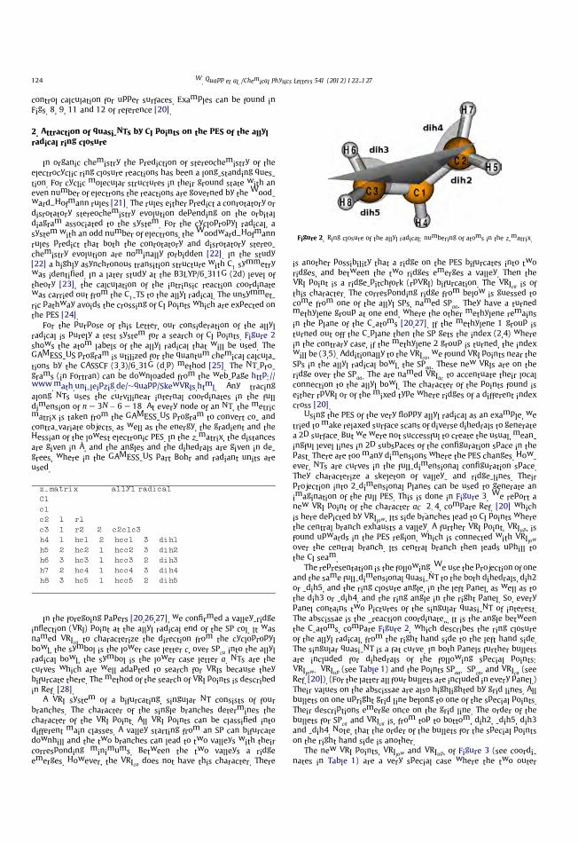
control calculation for upper surfaces. Examples can be found inFigs. 8, 9, 11 and 12 of reference [20].
2. Attraction of quasi-NTs by CI points on the PES of the allyl
radical ring closure
In organic chemistry the prediction of stereochemistry of theelectrocyclic ring closure reactions has been a long-standing ques-tion. For cyclic molecular structures in their ground state with aneven number of electrons the reactions are governed by the Wood-ward–Hofmann rules [21]. The rules either predict a conrotatory ordisrotatory stereochemistry evolution depending on the orbitaldiagram associated to the system. For the cyclopropyl radical, asystem with an odd number of electrons, the Woodward–Hofmannrules predict that both the conrotatory and disrotatory stereo-chemistry evolution are nominally forbidden [22]. In the study[22] a highly asynchronous transition structure with C1 symmetrywas identified. In a later study at the B3LYP/6-311G (2d) level oftheory [23], the calculation of the intrinsic reaction coordinatewas carried out from the C1-TS to the allyl radical. The unsymmet-ric pathway avoids the crossing of CI points which are expected onthe PES [24].
For the purpose of this Letter, our consideration of the allylradical is purely a test system for a search of CI points. Figure 2shows the atom labels of the allyl radical that will be used. TheGAMESS-US program is utilized for the quantum chemical calcula-tions by the CASSCF (3,3)/6-31G (d,p) method [25]. The NT-pro-grams (in Fortran) can be downloaded from the web-page http://www.math.uni-leipzig.de/$quapp/SkewVRIs.html. Any tracingalong NTs uses the curvilinear internal coordinates in the fulldimension of n ¼ 3N À 6 ¼ 18. At every node of an NT, the metricmatrix is taken from the GAMESS-US program to convert co- andcontra-variate objects, as well as the energy, the gradient and theHessian of the lowest electronic PES. In the z-matrix, the distancesare given in Å, and the angles and the dihedrals are given in de-grees, where in the GAMESS-US part Bohr and radiant units areused.
z-matrix allyl radical
C1
c1
c2 1 r1
c3 1 r2 2 c2c1c3
h4 1 hc1 2 hcc1 3 dih1
h5 2 hc2 1 hcc2 3 dih2
h6 3 hc3 1 hcc3 2 dih3
h7 2 hc4 1 hcc4 3 dih4
h8 3 hc5 1 hcc5 2 dih5
In the foregoing papers [20,26,27], we confirmed a valley-ridgeinflection (VRI) point at the allyl radical end of the SP col. It wasnamed VRIca to characterize the direction from the cyclopropylbowl, the symbol is the lower case letter c, over SPca into the allylradical bowl, the symbol is the lower case letter a. NTs are thecurves which are well adapted to search for VRIs because theybifurcate there. The method of the search of VRI points is describedin Ref. [28].
A VRI system of a bifurcating, singular NT consists of fourbranches. The character of the single branches determines thecharacter of the VRI point. All VRI points can be classified intodifferent main classes. A valley starting from an SP can bifurcatedownhill and the two branches can lead to two valleys with theircorresponding minimums. Between the two valleys a ridgeemerges. However, the VRIca does not have this character. There
is another possibility that a ridge on the PES bifurcates into tworidges, and between the two ridges emerges a valley. Then theVRI point is a ridge-pitchfork (rpVRI) bifurcation. The VRIca is ofthis character. The corresponding ridge from below is guessed tocome from one of the allyl SPs, named SPaa. They have a turnedmethylene group at one end, where the other methylene remainsin the plane of the C-atoms [20,27]. If the methylene 1 group isturned out off the C-plane then the SP gets the index (2,4) wherein the contrary case, if the methylene 2 group is turned, the indexwill be (3,5). Additionally to the VRIca, we found VRI points near theSPs in the allyl radical bowl, the SPaa. These new VRIs are on theridge over the SPaa. The are named VRIac to accentuate their localconnection to the allyl bowl. The character of the points found iseither rpVRI or of the mixed type where ridges of a different indexcross [20].
Using the PES of the very floppy allyl radical as an example, wetried to make relaxed surface scans of diverse dihedrals to generatea 2D surface. But we were not successful to create the usual, mean-ingful level lines in 2D subspaces of the configuration space in thepast. There are too many dimensions where the PES changes. How-ever, NTs are curves in the full-dimensional configuration space.They characterize a skeleton of valley- and ridge-lines. Theirprojection into 2-dimensional planes can be used to generate animagination of the full PES. This is done in Figure 3. We report anew VRI point of the character ac 2;4, compare Ref. [20] whichis here depicted by VRIlow. Its side branches lead to CI points wherethe central branch exhausts a valley. A further VRI point, VRIup, isfound upwards in the PES region, which is connected with VRIlowover the central branch. Its central branch then leads uphill tothe CI seam.
The representation is the following.We use the projection of oneand the same full-dimensional quasi-NT to the both dihedrals, dih2or -dih5, and the ring closure angle, in the left panel, as well as tothe dih3 or -dih4, and the ring angle in the right panel. So, everypanel contains two pictures of the singular quasi-NT of interest.The abscissae is the ‘‘reaction coordinate’’. It is the angle betweenthe C-atoms, compare Figure 2, which describes the ring closureof the allyl radical, from the right hand side to the left hand side.The singular quasi-NT is a fat curve. In both panels further bulletsare included for dihedrals of the following special points:VRIlow; VRIup (see Table 1) and the points SPaa; SPca, and VRIca (seeRef. [20]). (For the latter all four bullets are included in every panel.)Their values on the abscissae are also highlighted by grid lines. Allbullets on one upright grid line belong to one of the special points.Their descriptions emerge once on the grid line. The order of thebullets for SPca and VRIca is, from top to bottom, dih2, -dih5, dih3and -dih4. Note, that the order of the bullets for the special pointson the right hand side is another.
The new VRI points, VRIlow and VRIup, of Figure 3 (see coordi-nates in Table 1) are a very special case where the two outer
Figure 2. Ring closure of the allyl radical: numbering of atoms in the z-matrix.
124 W. Quapp et al. / Chemical Physics Letters 541 (2012) 122–127
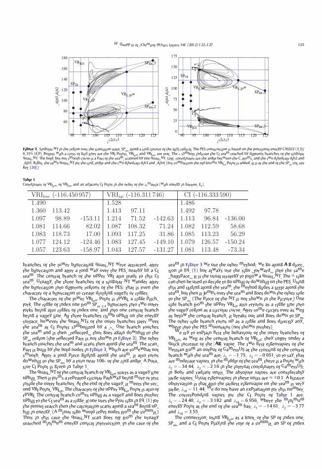
branches of the lower bifurcating quasi-NT were attracted, afterthe bifurcation and after a long way over the PES, nearby by a CIseam. The central branch of the upper VRI also leads to this CIseam. Usually, the three branches of a singular NT wander afterthe bifurcation into different regions of the PES; that is even thecharacter of a bifurcation to create dividing valleys or ridges.
The character of the lower VRIlow point is rpVRI, a ridge pitch-fork. The ridge of index one from SPaa 2;4 bifurcates into two outerforks being also ridges of index one, and into one central branchbeing a valley line. All three branches climb uphill on the energysurface, however the quasi-NTs of the outer branches later meetthe seam at CI points symbolized by a ‘Ã’. One branch touchesthe seam and is then ‘‘reflected’’, thus goes again downhill to theSPaa region (the reflected part is not shown in Figure 3). The otherbranch touches the seam and scans then along the seam. The scan-part is built by the bold nodes in Figure 3, which are somewhat notsmooth. After a long piece gliding along the seam, it also turnsdownhill to the SPaa, by a turn near 106� of the ring angle. A puta-tive CI point is given in Table 1.
The quasi-NT of the central branch of VRIlow starts as a valley lineuphill. Then it forms a repeated circular pathway beingmore or lessinside the outer branches. At the end of the valley, it meets the sec-ond VRI point, VRIup. The character of the upper VRIup point is also ofrpVRI. The central branch comes uphill as a valley and goes furtheruphill to the CI seam as a ridge. If one uses the plus sign in Eq. (1) forthe funnel search then the calculation scans along a seam going up-hill in energy. (A minus sign would repel nodes from the summit.)Thus in this case the quasi-NT scan goes off from the usuallysearched minimum energy conical intersection. In the case of the
seam in Figure 3 we use the other method: we go along A g direc-tion in Eq. (1) but always use the sign ‘‘forward’’, into the same‘‘halfspace’’. It is the usual strategy to follow a quasi-NT. The Æ signcan then be used to decide to go uphill or downhill on the PES. Usingthis and sliding along the seam, the method glides a little along theseam, but then it jumps over the seam and goes down the other sideto the SPca. (The piece of the NT is not shown in the picture.) Oneside branch from the upper VRIup also returns as a ridge line intothe valley region as a circular curve. After some circles over as wellas below the central branch, it breaks out and goes down to SPaa.The other side branch turns up as a ridge and goes directly any-where into the PES mountains (not shown further).
We try to explain first the behaviour of the outer branches ofVRIlow, as well as the central branch of VRIup: they suffer under aquick increase of the jAgj value. The two first eigenvalues of theHessian from an output of GamessUS at the crossing of the centralbranch with the seam are: k1 ¼ À1:75; k2 ¼ À0:051, so to say, thataremoderate values. In themiddle of the seam, there is a point withk1 ¼ À34:44; k2 ¼ À2:16 in the internal coordinates of GamessUS:in Bohr and radiant units. The absolute values are considerablylarge values. Usual eigenvalues in these units are % Æ0:1. A bizarreobservation is that also the largest eigenvalue on the seam is verylarge: k18 ¼ 11:44. We do not have an explanation for this number.The corresponding values for the CI point of Table 1 are:k1 ¼ À24:40; k2 ¼ À3:182 and k18 ¼ 6:956, where the minimumenergy point at the end of the seam has: k1 ¼ À14:61; k2 ¼ À3:77and k18 ¼ 3:55.
The connection, using VRIlow as a knot, of the SP of index one,SPaa, and a CI point playing the role of a summit, an SP of index
90 95 100 105 110 115 120 125c2c1c3
60
80
100
120
140
160
180dih5dih2
CI
SPaa_5
SPaa_2
VRI_low
VRI_up
SPca
VRIca
90 95 100 105 110 115 120 125c2c1c3
0
25
50
75
100
125
150
175
dih4dih3
SPaa_4
SPaa_3
VRI_lowVRI_up
SPca
VRIca
CI
CI
Figure 3. Singular NT in the region over the transition state, SPaa , along a ring closure of the allyl radical. The PES construction is based on the functional energy CASSCF (3,3)/6-31G (d,p). Bullets with a cross of grid lines are the VRI points, VRIlow and VRIup , see text. The à symbols indicate the CI seam reached by different branches of the singularquasi-NT. The bold, but not smooth curve is a part of the seam, scanned by one quasi-NT. Left: coordinates are the angle between the C-atoms, and the two dihedrals dih2 and-dih5. Right: the same quasi-NT for the ring-angle and the two dihedrals dih3 and -dih4. (For comparison the old known VRIca point is added. It is at the end of the SPca col, seeRef. [20].)
Table 1
Coordinates of VRIlow , of VRIup , and an adjacent CI point in the order of the z-matrix (with energy in hartree, Eh).
W. Quapp et al. / Chemical Physics Letters 541 (2012) 122–127 125

two, by the outer branches of the quasi-NT of VRIlow shows anindex difference by one. It does not violate the index theorem forNTs [29,30] that a regular NT (without a VRI point) cannot connecttwo stationary points of the same index.
We guess that the CI points of the seam have a peaked topology[31], because we find two negative eigenvalues of the Hessianthere. A further hint for a peaked topology is the following: differ-ent steepest descent pathways from the putative CI points go intoaccidental directions. It is a hint that such a point is like a summit.For a sloped CI, the direction would be fixed. The found CI pointsare not symmetric in the dihedrals. However, the distances r1and r2 cross near some CI points their symmetry line atr1 ¼ r2 ¼ 1:492 8. One should compare other symmetric CIs foundin Refs. [32,33].
We guess that the growing string of the special branches of thesingular quasi-NT meet the CI seam (by accident) anywhere andthen we can jump over it, or we can scan along the CI seam withthe quasi-NT. The condition for meeting the seam at all is thatthe search direction of the current quasi-NT fulfills the equation
1=Norm à ð½vc vcT þ vd vdT �gÞ ¼ r; ð10Þ
being r the selected direction by the actual NT with Eq. (1). 1=Normis a normalization constant, and vc, vd are the vectors of thebranching Tb subspace, see Eqs. (7) and (8). Using the ‘‘forward’’strategy along the seam by a search direction with formula (10),we can descend to a putative minimum energy point on the conicalintersection seam at 106� of the ring angle, see Figure 3. The energydifference of the first seam crossing point of the three branches ofthe singular quasi-NT, and the minimal node, is from À116:28 Ehto À116:37 Eh, see Figure 4. At all, one should keep in mind that aquasi-NT slips from one true NT to another, step by step, and itcan therefore end up at a different search direction than the NT itstarted from (though our predictor step length is very small). Figure3 suggests that the branch connecting VRIup with SPaa does not be-long to the same NT as the branch that connects SPaa and VRIlow.However it emerges to a miracle that the central branch connectsthe VRIlow with the VRIup.
A control calculation at a putative CI point of the seam, seeTable 1, was done. A CASCI calculation of the corresponding firstexcited electronic surface, eA2B, at this configuration confirms theconjecture to be at a CI point: It is based on the natural orbitalsextracted from the CAS (3,3) (quartet) set. The energy differencebetween the two doublet states is 0.5 kcal/mol, it is an excellentvalue. The description of the three states is
state 1: energy ¼ À116:328 448 481; S ¼ 0:5,state 2: energy ¼ À116:327 647 388; S ¼ 0:5,state 3: energy ¼ À116:315 182 186; S ¼ 1:5,and SZ ¼ 0:5, space sym ¼ A holds in all three cases.
The central branch of the lower VRI point, VRIlow, needs a secondexplanation, as well as the existence of the upper VRIup crossed byone singular NT. The lower central branch circulates five and a halftimes around a valley of the PES, up to the upper VRI point. Thecircular curves implicate the possibility that an NT can be quiteconvoluted on a hilly PES. In each case the uphill pathway is avalley line going up to a turning point, where the quasi-NT turnsand goes parallel downhill. Then this pathway is a ridge line goingdown back to the initial region. And so on, five and a half rounds upto VRIup.
There is a simplified analogy to a circular NT on a simple2-dimensional surface, see the right panel of Figure 5 which maybe compared with Fig. 3.11 of Ref. [30], the so-called dent of a
0 50 100 150 200
nodes
116.45
116.425
116.4
116.375
116.35
116.325
116.3
116.275
Energy
VRI_low
VRI_upseam
SPaa
SPca
Figure 4. Energy profile along an outer branch of the singular quasi-NT in VRIlow ,along a ring closure of the allyl radical, up to the CI seam, then gliding downhillalong the seam, and then going downhill back to SPaa. (The last piece of the quasi-NT is not shown in Fig. 3.) Bullets depict the energy of special points, likeVRIlow; VRIup; SPca and SPaa.
2 1 0 1 2x
1
0
1
2
3
y
CI
SP
VRI VRI
niMniM
SP SP
2 1 0 1 2x
1
0
1
2
3
y
Figure 5. NTs connect stationary points. Left: A ridge to a CI point at (0,2). Two singular NTs connect the two minimums with the CI point which plays the role of a summit.Right: Compact NTs emerge inside the dent of a thumb on the ridge. A further singular NT emerges with two VRIs on the y-axis (bold dashes).
126 W. Quapp et al. / Chemical Physics Letters 541 (2012) 122–127

thumb. Maybe that the example can explain the behaviour of thecircular pieces of the NT in Figure 3. The formula of a 2-dimen-sional toy surface on the left hand side is
slðx; yÞ ¼ x2 ðx2 À 2þ 1:5 yÞ þ y2 ðyÀ 4Þ2 À 25ffiffiffiffiffiffiffiffiffiffiffiffiffiffiffiffiffiffiffiffiffiffiffiffiffiffiffiffiffiffiffiffix2 þ 3 ðyÀ 2Þ2
q
ð11Þ
and additionally, for the right panel a dent is pressed into the ridgeon the y-axis:
srðx; yÞ ¼ slðx; yÞ À 25 expðÀ3:48 x2 À 4 ðyÀ 1:093Þ2Þ: ð12Þ
The level lines of the PES are thin lines, where families of NTs arerepresented by bolder lines. In the left panel, a ‘‘usual’’ surface isdrawn. Here two singular NTs of the mixed type connect the twolower minimums with the CI point at the top crossing one of theVRI points, and the other branches connect different SPs. On theright panel, an additional dent is pressed into the ridge which leadsfrom the lower SP to the CI point. Now the VRIs are moved a little,and new compact NTs emerge. The dent on the slope of the ridgesurface is filled by a pair of families of compact NTs, and a newsingular NT (the dashes on the y-axis) divides the families. Thesingular NT crosses a lower VRI point at % ð0:0;0:2Þ, and a further,upper VRI point at % ð0:0;1:7Þ. Both VRIs are rpVRIs. The inner,circular NTs inside the dashed, singular NT do not cross stationarypoints or VRIs. They are compact curves. Note, the molecular caseon the PES in Figure 3 may be a little more complicated. There are18 dimensions for the PES. The central branch of the singular NTis a spiral line which cannot be in a 2-dimensional plane. Notefurther that the CI points first found must not be a minimum, oran SP on the high-dimensional seam, compare the Refs. [31,34].
3. Conclusion
Up to date, the calculation of CI points is a difficult job, see ref-erences [4–6] and further references therein. We have ‘‘simply’’used the numerical following along quasi-NTs on the ground adia-batic PES and this leads to peaked CI points quite in analogy to thefinding of SPs of index 2 [8,9]. The coordinates of a pututive CI pointon the allyl radical PES are given in Table 1. We think that we didnot find the exact CI, however the point is assumed to be near theapex of the corresponding conoid. In Figure 3 we depict the projec-tion of quasi-NTs into 2-dimensional planes. Even though quasi-NTs are curves in the full-dimensional configuration space, weassume that we can use their projections for four different, butimportant dihedrals to generate an imagination of the PES. NTscharacterize a skeleton of valley- and ridge-lines. They bifurcatewhere valleys or ridges of the PES bifurcate. In the case discussedhere, we find that a long valley exists on the ridge on the allylradical PES (without an intermediate minimum), if one leaves theSPaa uphill in a corresponding ridge direction. The lower entrance
into the valley goes through a VRI point. The upper departure gateis also a VRI point like in Figure 5. On the high-dimensional PES, thepathway of the central branch leaves the valley and later crosses theCI seam, as well as the two lower side branches. At the top near theformer valley, a long CI seam is placed. The new avenue to find thestructures is the Newton trajectory method.
Acknowledgments
Financial support from the Spanish Ministerio de Economía yCompetitividad, DGI project CTQ2011-22505 and, in part fromthe Generalitat de Catalunya projects 2009SGR-1472 is fullyacknowledged. M.C. gratefully thanks the Ministerio de Economíay Competitividad for a predoctoral fellowship.
We thank two referees for many helpful suggestions andcomments.
References
[1] D. Heidrich (Ed.), The Reaction Path in Chemistry: Current Approaches andPerspectives, Kluwer, Dordrecht, 1995.
[2] D.R. Yarkony, Rev. Mod. Phys. 68 (1996) 985.[3] M.J. Bearpark, M.A. Robb, H.B. Schlegel, Chem. Phys. Lett. 223 (1994) 269.[4] J.M. Anglada, J.M. Bofill, J. Computat. Chem. 18 (1996) 992.[5] F. Sicilia, L. Blancafort, M.J. Bearpark, M.A. Robb, J. Theor. Chem. Computat. 4
(2008) 257.[6] S. Maeda, K. Ohno, K. Morokuma, J. Chem. Theor. Computat. 6 (2010) 1538.[7] I.H. Williams, G.M. Maggiora, J. Mol. Struct. (Theochem) 89 (1982) 365.[8] W. Quapp, M. Hirsch, D. Heidrich, Theor. Chem. Acc. 100 (1998) 285.[9] W. Quapp, M. Hirsch, O. Imig, D. Heidrich, J. Comput. Chem. 19 (1998) 1087.[10] W. Quapp, J. Comput. Chem. 22 (2001) 537.[11] M. Hirsch, W. Quapp, J. Comput. Chem. 23 (2002) 887.[12] J.M. Anglada, E. Besalu, J.M. Bofill, R. Crehuet, J. Comput. Chem. 22 (2001) 387.[13] J.M. Bofill, J.M. Anglada, Theor. Chem. Acc. 105 (2001) 463.[14] R. Crehuet, J.M. Bofill, J.M. Anglada, Theor. Chem. Acc. 107 (2002) 130.[15] W. Quapp, J. Mol. Struct. 695–696 (2004) 95.[16] J.M. Bofill, W. Quapp, J. Chem. Phys. 134 (2011) 074101.[17] F.H. Branin, IBM J. Res. Dev. 16 (1972) 504.[18] M. Hirsch, W. Quapp, J. Math. Chem. 36 (2004) 307.[19] P.-O. Löwdin, in: C.H. Wilcox (Ed.), Perturbation Theory and Its Application in
Quantum Mechanics, Wiley, New York, 1966, p. 255.[20] W. Quapp, J.M. Bofill, J. Math. Chem. (2012), http://dx.doi.org/10.1007/s10910-
012-9995-8.[21] R.B. Woodward, R. Hoffmann, J. Am. Chem. Soc. 87 (1965) 395.[22] S. Olivella, A. Solé, J.M. Bofill, J. Am. Chem. Soc. 112 (1990) 2160.[23] P.A. Arnold, B.K. Carpender, Chem. Phys. Lett. 328 (2000) 90.[24] Y. Haas, S. Cogan, S. Zilberg, Int. J. Quant. Chem. 102 (2005) 961.[25] Gamess-US program M.V. Schmidt et al., J. Comput. Chem. 14 (1993) 1347.[26] A. Aguilar-Mogas, X. Giménez, J.M. Bofill, J. Comput. Chem. 31 (2010) 2510.[27] W. Quapp, J.M. Bofill, A. Aguilar-Mogas, Theor. Chem. Acc. 129 (2011) 803.[28] W. Quapp, B. Schmidt, Theor. Chem. Acc. 128 (2011) 47.[29] I. Diener, Globale Aspekte des kontinuierlichen Newtonverfahrens,
Habilitation, Universität Göttingen, Germany, 1991.[30] M. Hirsch, Dissertation (Ph.D. Thesis), Universität Leipzig, Germany, 2004.[31] G.J. Atchity, S.S. Xanteas, K. Ruedenberg, J. Chem. Phys. 95 (1991) 1862.[32] L. Castiglioni, A. Bach, Phys. Chem. Chem. Phys. 8 (2006) 2591.[33] M. Shahu, Int. J. Quant. Chem. 106 (2006) 501.[34] F. Sicilia, L. Blancafort, M.J. Bearpark, M.A. Robb, J. Phys. Chem. A 111 (2007)
2182.
W. Quapp et al. / Chemical Physics Letters 541 (2012) 122–127 127
Locating transition states on potential energy surfaces by the gentlestascent dynamics
Josep Maria Bofill a,b,⇑, Wolfgang Quapp c, Marc Caballero b,d
aDepartament de Química Orgànica, Universitat de Barcelona, Martí i Franquès, 1, 08028 Barcelona, Spainb Institut de Química Teòrica i Computacional, Universitat de Barcelona, (IQTCUB), Martí i Franquès, 1, 08028 Barcelona, SpaincMathematisches Institut, Universität Leipzig, PF 100920, D-04009 Leipzig, GermanydDepartament de Química Física, Universitat de Barcelona, Martí i Franquès, 1, 08028 Barcelona, Spain
a r t i c l e i n f o
Article history:
Received 13 June 2013
In final form 26 July 2013
Available online 2 August 2013
a b s t r a c t
The system of ordinary differential equations for the method of the gentlest ascent dynamics (GAD) has
been derived which was previously proposed [W. E and X. Zhou, Nonlinearity 24, 1831 (2011)]. For this
purpose we use diverse projection operators to a given initial direction. Using simple examples we
explain the two possibilities of a GAD curve: it can directly find the transition state by a gentlest ascent,
or it can go the roundabout way over a turning point and then find the transition state going downhill
along its ridge. An outlook to generalised formulas for higher order saddle-points is added.
� 2013 Elsevier B.V. All rights reserved.
1. Introduction
The concepts of the potential energy surface (PES) [1,2] and of
the chemical reaction path are the basis for the theories of chemi-
cal dynamics. The PES is a continuous function with respect to the
coordinates of the nuclei. It is an N-dimensional hypersurface if
N = 3n and n is the number of atoms. It must have continuous
derivatives up to a certain order.
The PES can be seen as formally divided in catchments associ-
ated with local minima [1,3]. The first order saddle points or tran-
sition states (TSs) are located at the deepest points of the boundary
of the basins. Two neighbouring minima of the PES can be con-
nected through a TS via a continuous curve in the N-dimensional
coordinate space. The curve characterises a reaction path. One
can define many types of curves satisfying the above requirement.
The reaction path model widely used is the steepest descent (SD).
There exist a large number of proposed methods that in princi-
ple reach a TS when the minimums associated to the reactant and
product are known. See Ref. [4] and references therein. There are
also methods that find the TS when only one minimum is known.
In this case, the problem is much more cumbersome because the
initial data are just the geometry coordinates of the minimum,
however, the direction of the search is open. As in the first case
many algorithms have been developed for this type of problem
[4]. A great number of these algorithms are based in a generalisa-
tion of the Levenberg–Marquardt method [5–7] that basically con-
sists of a modification of the Hessian matrix to achieve both, first
the correct spectra of the desired Hessian at the stationary point,
and second to control the length of the displacement during the
location process. The first proposed algorithm within this philoso-
phy is due to Scheraga [8] and from than up to now the list is very
large [9–20]. None of the methods are foolproof, each of them has
some problems. Recently E and Zhou [20] have proposed an ap-
proach called the ‘gentlest ascent dynamics’ method. This method
can be seen as a new reformulation of the method proposed some
time ago by Smith [12,13] under the name ‘image function’. The
method is based on the generation of an image function that is a
function which has its minima at exactly the points where the ori-
ginal PES has its TSs and moreover by an application of a minimum
search algorithm to this image function. The converged point
should correspond to a TS in the actual PES. Helgaker [14] modified
the algorithm by the trust radius technique. Sun and Ruedenberg
[21] analysed the method concluding that image functions do not
exist for general PES so that a plain minimum search is inappropri-
ate for them. A nonconservative field gradient of the image func-
tion exists. The global structure of the image gradient fields is
considerably more complex than that of gradient fields of the ori-
ginal function. However, the image gradient fields appear to have
considerably larger catchment basins around TSs. Besalú and Bofill
[18] showed that the Smith algorithm is a special type of the
Levenberg–Marquardt method.
In this Letter we show the connection between the Smith meth-
od [12,13] and that described by E and Zhou [20] to find TSs, and
additionally, the mathematical basis of this algorithm is discussed.
Finally, some examples are reported.
0009-2614/$ - see front matter � 2013 Elsevier B.V. All rights reserved.
http://dx.doi.org/10.1016/j.cplett.2013.07.074
⇑ Corresponding author at: Departament de Química Orgànica, Universitat de
Barcelona, Martí i Franquès, 1, 08028 Barcelona, Spain. Fax: +34 933397878.
E-mail address: [email protected] (J.M. Bofill).
Chemical Physics Letters 583 (2013) 203–208
Contents lists available at ScienceDirect
Chemical Physics Letters
journal homepage: www.elsevier .com/ locate /cplet t
2. Background of the method
Let us denote by V(q) the PES function and by qT = (q1, . . ., qN)
the coordinates. The dimension of the q vector is N. The superscript
T means transposition. At every interesting point q the PES func-
tion admits a local gradient vector, g(q) =rqV(q), and a Hessian
matrix,H(q) =rqrqTV(q). The family of image functions of V(q), la-
belled by W(q), is defined by the differential equation [21]
fðqÞ ¼ UvgðqÞ ¼ IÀ 2vðqÞvTðqÞ
vTðqÞvðqÞ
� �
gðqÞ ð1Þ
where f(q) is the image gradient vector, Uv is the Householder
orthogonal matrix constructed by an arbitrary vector v(q) being in
principle a function of q, and I is the unit matrix. The Householder
orthogonal matrix is a reflection at v(q). It has the property that
Uv = UvT, and it is the result of the difference between the projectors
(I À Pv) and Pv, because it holds trivially Uv = I À 2Pv = (I À Pv) À Pv,
being Pv the projector that projects into the subspace spanned by
the v-vector [22]. If the derivatives of v(q) with respect to q are non-
vanishing, the image Hessian matrix, F(q) = UvH(q), is not obtained
by the differentiation of f(q). Taking into account Eq. (1), this differ-
entiation results in
rqfTðqÞ ¼ rqðg
TðqÞUvÞ ¼ FTðqÞ þ gTðqÞrqUv
¼ FTðqÞ À 2gTðqÞrq
vðqÞvTðqÞ
vTðqÞvðqÞ
� �
: ð2Þ
The term in brackets is usually not zero and not symmetric, and
this non-symmetry is due to the effect of the differentiation on the
Pv projector. In other words,
rqfTðqÞ
� �
ijÀ rqf
TðqÞ
� �
ji¼ rqf
TðqÞ
� �
ij
À rqfTðqÞ
� �T
ij–0 i–j: ð3Þ
The inequality of Eq. (3) implies that the image gradient field
defined by Eq. (1) is not integrable to an ‘image PES’ W(q). More
explicitly,
Wðq1Þ ÀWðq0Þ–
Z t1
t0
fTðqÞðdq=dtÞdt ð4Þ
where dq/dt is the tangent of an arbitrary curve joining the points
q0 = q(t0) and q1 = q(t1). Due to Eq. (3), this gradient field vector
should be considered as a nonconservative force field. From this fact
it follows an image of the PES function does, in general, not exist
[21,23].
From Eq. (3) it is easy to see that at the stationary points, where
g(q) = 0, the inequality is transformed to an equality if the v-vector
is an eigenvector of the Hessian matrix. Note that if {h, v/(vTv)1/2} is
an eigenpair of the H(q) matrix, then F(q) = UvH(q) = (I – 2vvT/
(vTv)) H(q) = H(q) - 2vvT/(vTv) h = H(q) - h 2vvT/(vTv) = H(q) -
H(q) 2vvT/(vTv) = H(q) (I – 2vvT/(vTv)) = H(q)Uv = FT(q). As pointed
out by Sun and Ruedenberg [21], the image functions do exist until
the second order in the vicinity of its stationary points for any PES
taking v as an eigenvector of the Hessian matrix. Due to this fact
the SD curves of the quadratic image function are approximations
to the gradient image curves of W(q) being the image potential of
V(q).
With the previous analysis of the general nonexistence of an
image PES, we can take the image gradient field given in Eq. (1)
to define the field of SD curves as,
dq
dt¼ ÀfðqÞ ¼ ÀUvgðqÞ ¼ À½ðIÀ PvÞ À Pv �gðqÞ ð5Þ
where t is the parameter that characterises the SD curve, q(t). If Eq.
(5) is multiplied consecutively from the left by the set of (N-1) linear
independent orthogonal vectors to the v-vector, we see that it cor-
responds to a curve which is energy descending along this set of
directions on the actual PES, whereas is ascending on the v-vector
direction. This property makes the set of curves defined in Eq. (5)
suitable for the location of a TS from a minimum. This observation
is supported by the fact that Eq. (5) can be rewritten as
dq
dt¼ À½ðIÀ PvÞ À Pv �gðqÞ ¼ ÀðIÀ PvÞgðqÞ þ PvgðqÞ
¼ ÀðIÀ PvÞgðqÞ þ lv
ðvTvÞ
1=2ð6Þ
being l = vTg(q)/(vTv)1/2, where the definition of Pv has been used.
Eq. (6) is the basic equation of the string method proposed for the
location of reaction paths and TSs [24]. The v-vector in this method
is the current tangent of the path. Because we are interested to find
TSs from minimums of the PES we can use the nonconservative
property of the gradient image field to modify the v-vector, during
the location process. For this purpose, we first consider that at the
minimum, as well as at the TS, the last term of the right hand side
part of Eq. (2) is equal zero due to g(q) = 0. Second, at the TS, the
Hessian matrix, H(q), possesses only one eigenpair with negative
eigenvalue. The associated Raygleigh-Ritz quotient of this eigenpair
with a negative eigenvalue is the lowest that the Hessian matrix can
achieve at this point being equal to the corresponding eigenvalue
[25]. The Raygleigh-Ritz quotient for a given vector v and matrix
H is defined as, k(v) = vTHv/(vTv). The structure of this eigenvector
is unknown. To find the TS one should, however, ensure that during
the research process the path walks through the PES (given until
second order) such that the character of the surface becomes closer
to a first order saddle point. Taking into account these two consid-
erations we transform Eq. (3) imposing that g(q) = 0 at each point of
the search and multiplying the resulting equation from the left by (I
– Pv) and from the right by Pv,
1
2ðIÀ PvÞ rqf
TðqÞ
� �
À rqfTðqÞ
� �T� �
Pv
�
�
�
�
gðqÞ¼0
¼1
2ðIÀ PvÞ½HðqÞUv À UvHðqÞ�Pv ¼ ÀðIÀ PvÞHðqÞPv: ð7Þ
The effect of this multiplication by the projectors, (I-Pv) and Pv,
is that the resulting Eq. (7), multiplied from the right by the v-vec-
tor, is the gradient of the Rayleigh–Ritz quotient with respect to
this vector. If the v-vector is an eigenvector of the H(q) matrix then
the right hand side part of Eq. (7) is equal zero because every
eigenvector extremises the corresponding Rayleigh–Ritz quotient.
We will denote the Rayleigh–Ritz quotient by kq(v) to indicate its
dependence on q through the Hessian matrix. If a v-vector makes
the gradient of the Rayleigh–Ritz quotient equal zero then this vec-
tor is an eigenvector of the H(q) matrix and the value of the Ray-
leigh–Ritz quotient coincides with the corresponding eigenvalue
of the H(q) matrix. These properties suggest that a v-vector can
be changed following the SD direction of the Rayleigh–Ritz quo-
tient gradient with respect to v,
dv
dt¼ À
vTv
2rvkqðvÞ ¼ ÀðIÀ PvÞHðqÞPvv ð8Þ
Eq. (8) is also a function of q through the Hessian matrix. The
Rayleigh–Ritz quotient of the new v-vector obtained from,
v? v + dv/dt Dt, will be lower with respect to the previous one
and, in addition, Eq. (5) will give us a new energy ascent direction
and a set of orthogonal N-1 energy descent directions. Eq. (8)
searches for either the lowest positive or the single negative Ray-
leigh–Ritz quotient if it exists, whereas Eq. (5) determines points
on the PES along the action of an increase of the energy in the v-
vector, and a decrease along the set of orthogonal directions to this
vector. The specific action of Eq. (5) defines the type of points of the
204 J.M. Bofill et al. / Chemical Physics Letters 583 (2013) 203–208

PES so that its structure until the second order on q resembles a
first order saddle point. In turn, Eq. (8) finds v-vectors with lowest
or possibly negative values of the Rayleigh–Ritz quotients of the
corresponding Hessian matrix. These two coupled actions on the
Eq. (5) and Eq. (8) describe a gradually or gentlest form to find
the TS located on the boundary of the basin which contains the
start minimum. Eqs. (5) and (8) are coupled since both depend
on the v-vector explicitly on q through the gradient vector and
the Hessian matrix respectively. The integration of Eqs. (5) and
(8) implies the solution of the differential equation
dqdt
dvdt
!
¼ ÀIÀ 2 vvT
vTv
� �
gðqÞ
IÀ vvT
vTv
� �
HðqÞv
0
B
@
1
C
Að9:aÞ
with the initial conditions
qðt0Þ
vðt0Þ
� �
¼q0
gðq0Þ
� �
ð9:bÞ
where q0 is a slightly distorted point near the minimum. The gradi-
ent at point q0 is selected automatically as the initial v-vector. Eqs.
(9) are the basic expressions of the algorithm proposed by E and
Zhou [20] which are reviewed in this study.
Note that the system (9) is a system of differential equations.
Corresponding to the initial conditions (9b) there emerges a full
family of solution curves passing every point of a given region. This
is in contrast to the long known gradient extremals (GE). They also
realize a shallowest ascent idea; however, they are special solution
curves of the equation Hg = kg, where k is an eigenvalue of H. Thus
the GEs pass only points where the gradient itself is an eigenvector
of H [2,26–31]. GEs do not cover a region.
3. Behaviour and analysis
The set of Eqs. (9) has been integrated using the explicit Runge–
Kutta method of order 8(5,3) [32]. We have used two-dimensional
PES models to analyse the behaviour of the gentlest ascent path.
The first PES model used for this purpose is the Wolfe-Quapp PES
[33,34]. The equation of this surface model is
Vðx; yÞ ¼ x4 þ y4 À 2x2 À 4y2 þ xyþ 0:3xþ 0:1y ð10Þ
We look for the gentlest ascent dynamics if we start from the min-
imum located at the point (1.124,À1.486) with energy in arbitrary
units À6.369. We take the corresponding gradient vector there as a
starting point (1.2,À1.5) and as the initial v-vector, according to Eq.
(9.b). The curve line is depicted in Figure 1. It starts from the min-
imum. The curve ends at the TS located in (0.093,0.174) with en-
ergy À0.644. It follows the valley joining these two stationary
points. Figure 1 also shows the behaviour of the v-vector. Initially
the v-vector has the same direction to the tangent of the curve
but along the initial sub-arc of the curve the vector points to the
direction where the energy increases very fast, and finally the vec-
tor corrects its direction towards the direction of the transition vec-
tor. The transition vector is the eigenvector of the Hessian matrix at
the TS with the negative eigenvalue. At the end point, namely the
TS, the v-vector is the vector which produces the lowest value of
the Rayleigh–Ritz quotient of the Hessian matrix. It is the eigen-
value of the transition vector. This behaviour conforms to that
one which is explained in the previous section. The curve is deter-
mined by the condition that the v-vector minimises the kq(v) within
the limits imposed by the Mini-Max eigenvalue theorem [25].
A second curve is computed on the same PES to get the same TS
revealing new features of this type of GAD curves. In this case the
curve starts near the minimum located at the point (À1.174,1.477),
with energy À6.762. The behavior of this curve is drawn in Figure
2. The path follows the valley in the direction where kq(v) takes the
possibly lowest value. The path arrives a highest energy value at a
turning point and starts to descend along a ridge, and it ends again
at the TS located at (0.093,0.174) with energy À0.644. As shown in
Figure 2, on a large sub-arc from the minimum the v-vector has the
same direction as the tangent of the curve. Of course, the large arc
with the turning point at its highest energy does not represent the
‘gentlest ascent’, seen from the TS and the valley nearby. So, the
name of the method, GAD, is a suggestive name but it is not rea-
lised in every case. However, note that the TS is in a side valley,
but the method finds the TS, in general. At the point
(1.849,0.635) the curve achieves the highest energy value and
starts its descents. This point is a turning point (TP) of the curve,
where the next equation is satisfied
Figure 1. Behaviour of the GAD curve on the Wolfe-Quapp PES model [33,34]. The
curve starts at point (1.2,À1.5) which is near to the minimum located at the point
(1.124,À1.486). The curve evolution ends at the TS located at point (0.093,0.174).
The set of v-vectors generated during the search is indicated by the set of bold
arrows.
Figure 2. Behaviour of the GAD curve on the Wolfe-Quapp PES model [33,34]. The
curve starts at the point near the minimum located at (À1.174,1.477). The curve
evolution ends at the TS located at the point (0.093,0.174). At the point
(1.849,0.635) the curve achieves the highest energy so this point is the TP. The
curve leaves the valley where the starting minimum is located at the point
(1.842,0.768). This point is a VRT point. The set of v-vectors generated during the
search are indicated by the set of bold arrows.
J.M. Bofill et al. / Chemical Physics Letters 583 (2013) 203–208 205

dV
dt¼ gT
dq
dt¼ ÀgTUvg ¼ ÀgTðIÀ PvÞgþ gTPvg ¼ 0 ð11Þ
where Eq. (5) has been used. In general a TP appears on the gentlest
ascent path when the square of the gradient norm in the subspace
spanned by the v-vector is equal to the square of the gradient norm
in the complementary subspace spanned by the set of linear inde-
pendent vectors orthogonal to the v-vector. This result is identical
to the equality gTg/2 = gTPvg, and with the definition of Pv we can
rewritten it as, 1/21/2 = gTv/(gTgvTv)1/2, concluding that the GAD
curve has a TP at the point where the v-vector and the gradient of
the actual PES form an angle of p/4 radians. The curve leaves the
valley where the starting minimum is located, at the point TP
(1.842,0.768) and it enters to a ridge region. Because this point sat-
isfies the next equations
gTAðqÞg
gTg¼ 0 ð12:aÞ
AðqÞg
ðgTgÞ1=2–0 ð12:bÞ
where A(q) is the adjoint matrix of the Hessian H(q) at the q point,
we conclude that this point is a valley–ridge transition point (VRT)
rather than a valley–ridge inflexion point (VRI) [35-37]. In a VRI
point both equations are equal zero. From the minimum to the
VRT point the curve shows positive values of the Rayleigh quotient,
gTAg/(gTg), whereas they are negative from the VRT point to the TS.
This quotient is taken as a convexity criterion of a PES region where
a point is located. Positivity of the quotient means that the point is
in a valley, otherwise it is on a ridge [38]. The result supports the
above comment, namely, that one sub-arc of the curve is located
in the deep valley from the minimum to the VRT point. At this point
the curve turns into the direction of the ridge following the lowest
value of kq(v). But this corresponds to the v-vector orthogonal to
both, the ascent of the valley and the descending ridge directions.
On the sub-arc located on the ridge at each point the gradient vector
increases its orthogonality with respect to the current v-vector. The
curve evolves along a direction of decreasing energy. We can write
dV/dt = gTdq/dt = ÀgTUvg = 2gTg((gTv)2/(gTg vTv) À 1/2) % ÀgTg < 0
since vTg % 0. In general the curve evolves so that the energy de-
creases at each step if the gradient vector g and the v-vector form
an angle within the open domains (p/4,3p/4) or (5p/4,7p/4)
radians.
In general we can mark the following features of a GAD curve.
When along the sub-arc of the gentlest ascent curve its gradient
vectors define an angle with the corresponding v-vectors within
the open domains (p/4,3p/4) or (5p/4,7p/4) radians, then the
sub-arc shows an energy decrease. If the angle is within the open
domains (3p/4,5p/4) or (7p/4,p/4) radians it shows an energy
growth. When the angle is equal to p/4, 3p/4, 5p/4, or 7p/4 radians
the curve is stationary with respect to the variation of the energy,
the TP situation.
The same type of calculations with the PES proposed by Neria
et al. [39] and modified by Hirsch and Quapp [38] confirms the
same facts. The equation of this surface model is
Vðx; yÞ ¼ 0:06ðx2 þ y2Þ2þ xyÀ 9expðÀðxÀ 3Þ2 À y2Þ
À 9expðÀðxþ 3Þ2 À y2Þ: ð13Þ
The central point is the TS located at (0,0) with energy À0.002.
The minima are located at (2.71,À0.15) and (À2.71,0.15) with en-
ergy À5.24. The surface has gorges around the points (2,À2) and
(À2,2) [38]. We start the gentlest ascent path at the point
(2.6,À0.2) near to a minimum. Its evolution goes over the gorge,
it leaves the valley where the minimum is located and it enters
the ridge, but then it enters again to the valley region of the min-
imum. The ascending energy behaviour ends at the point
(0.871,À1.428) being a TP. On the sub-arc between the points TP
and TS a VRT point exists at (0.002,À1.28) corresponding to the
descending energy. At this point the GAD curve enters a ridge that
touches the TS. Figure 3 depicts this behaviour, the evolution of the
v-vector is also shown.
On the Müller–Brown PES [40], the GAD method exhausts its
possibilities. The global minimum is located at a very deep valley.
The coordinates are (À0.56,1.44). We use two different starting
points. The first starting point of the GAD method is at the point
(À0.54,1.4) near to the minimum. The GAD trajectory leads to
the next TS, see Figure 4a where it is the dotted line. It goes over
a TP but that is normal. In Figure 4a we show the behavior of the
gradient extremal curve (GE) [2,26–31] for comparison. The GEs
are the bold dashed lines. A part of the GAD on the ridge coincides
with the GE. However, the coincidence is for different reasons. For
the GAD case, in the ridge region the v-vector is orthogonal to the
gradient and due to this fact the trajectory shows a decrease in en-
ergy. In other words, dV/dt is reduced, it is, dV/dt = ÀgTg < 0 since
vTg = 0. Recall that the v-vector evolves in this process to reach
the eigenvector of the Hessian matrix of lowest eigenvalue. Analyz-
ing the GE in the region of coincidence, the gradient at each point
of this curve is by construction an eigenvector of the Hessian cor-
responding to a positive eigenvalue. The eigenvalue is positive be-
cause its eigenvector comes from the evolution of the Hessian at
the TS labeled as SP1, in direction orthogonal to the col. For the
GE the variation energy is given by, dV/dt = (gTg)1/2eg, being eg a
component of the GE tangent equation [28,31] and depending of
its sign, the curve increases or decreases in energy. One can con-
clude that in the region of coincidence the v-vector is orthogonal
to the gradient vector, an eigenvector of the Hessian matrix. Thus,
the v-vector is in this region an eigenvector of the Hessian.
For a second trajectory we use the point (À0.58,1.427) for the
start, also near the minimum, however, we get a totally different
result, see Figure 4b. At the beginning, the GAD trajectory, a contin-
uous line, goes along the deep valley of the minimum, uphill like
the GE, which in Figure 4b is again represented by dashed lines,
see also Figure 2 of Ref. [28], or Figure 5 of Ref. [41]. The initial
evolution of GAD goes in the direction where the gradient and
Figure 3. Behaviour of the GAD curve on the Neria–Fischer–Karplus PES model [39]
modified according to that proposed by Hirsch and Quapp [38]. The curve starts at
point (2.6,À0.2) near the minimum located at (2.71,À0.15). The curve evolution
ends at the TS located at point (0,0). At point (0.871,À1.428) the curve achieves the
highest energy value. The point is the TP. The curve leaves the valley where the
starting minimum is located at the point (0.002,À1.28). This point is a VRT point.
The set of v-vectors generated during the search is indicated by the set of bold
arrows.
206 J.M. Bofill et al. / Chemical Physics Letters 583 (2013) 203–208
the v-vector form an angle lower than p/4 radians. In fact it coin-
cides with the GE, which in turn implies that the v-vector is paral-
lel to the gradient. In the region where both curves coincide the
increasing energy along the GAD curve is dV/dt = (gTv)2/vTv > 0.
The behavior ends at a TP which emerges near (À2.8,0) in a region
which is far away from the border line of the searched valley–ridge
transition. In Figure 14 of Ref. [38] the borders between valleys and
ridges of the Müller–Brown PES are shown. After the TP the trajec-
tory turns into the left large side valley of the Müller–Brown sur-
face. There is no stationary point, so GAD cannot find any one.
The region is a kind of a trap, a ‘dead’ valley. The GE passes the re-
gion and leaves it to the mountains at the left hand side, but the
GAD trajectory goes on and back, from one TP to the next, and
again back, and only by an accident, it later leaves the region. How-
ever, then it immediately leads to the TS2 of the Müller–Brown
surface. It seems to be accidentally which TS is found. After the
‘chaotic’ evolution, the GAD trajectory finally catches a TS.
4. A different view of the theory and generalisation
Mathematically the above method can be reformulated as
Maxv
Minw
fUðv;wÞjv ¼vTq;w¼ZTq and ZT
v¼ ½z1j . . . jzNÀ1�Tv¼0NÀ1g
where the v-vector satisfiesMinv
ÀvTHðqÞv
vTv
8
<
:
ð14Þ
where U(v,w) is the PES function, V(q), expressed as a function of
(v,w) coordinates being the w vector of dimension N-1. Finally,
the Z matrix is formed by a set of N-1 linear independent vectors
orthogonal to the v-vector. A suggested solution of the conditions
is formulated in Eq. (9). As noted, the method is appropriate for a
first-order saddle point search, and can be easily generalised to
the search of higher order saddle-points. The importance of second
order saddle-points is known [42,43]. If I is the order of the saddle-
point, where I 6 N, then the set of Eqs. (9) takes the form
dqdt
dv1dt
.
.
.
dvIdt
0
B
B
B
B
B
@
1
C
C
C
C
C
A
¼ À
IÀ 2X
I
i¼1
Pvi
!
gðqÞ
IÀX
I
i¼1
Pvi
!
HðqÞv1 þX
I
i¼1i–1
Pvi
!
HðqÞv1
.
.
.
IÀX
I
i¼1
Pvi
!
HðqÞvI þX
I
i¼1i–I
Pvi
!
HðqÞvI
0
B
B
B
B
B
B
B
B
B
B
B
B
B
@
1
C
C
C
C
C
C
C
C
C
C
C
C
C
A
ð15:aÞ
with the initial conditions
qðt0Þ
v1ðt0Þ
.
.
.
vIðt0Þ
0
B
B
B
B
@
1
C
C
C
C
A
¼
q0
gðq0Þ
.
.
.
pI0
0
B
B
B
B
@
1
C
C
C
C
A
ð15:bÞ
where Pvi = viviT/(vi
Tvi) for i = 1, ..., I, and {p0i}i=2
I is a set of I-1 orthog-
onal vectors which are orthogonal to the vector g(q0). If I = N then
the identity matrix I in Eq. (15.a) should be substituted by the res-
olution of identity
I ¼X
N
i¼1
Pvi : ð16Þ
The variation energy through this curve is given by
dV
dt¼ ÀgT
dq
dt¼ ÀgTðIÀ 2
X
I
i¼1
Pvi Þg ¼ 2X
I
i¼1
ðgTviÞ2
gTgvTi vi
À1
2
!
gTg ð17Þ
where the first N components of Eq. (15.a) have been used. Eq. (17)
tells us that when the sum of the square of the components of the
projected gradient vector in the subspace spanned by the set of vi-
vectors is higher than 1/2 then the curve evolves in the direction of
increasing the energy. If it is lower than 1/2 then evolves in the
direction of a decrease of energy. When the sum is equal to 1/2
the curve is at a TP.
5. Conclusion
In this study is reviewed the GAD method for the location of the
saddle points which surround a given minimum. It behaves like a
growing string method. The integration of the curve can be done
by any method suitable to integrate a system of first order ordinary
differential equations. The GAD constructs a curve supported by a
Min
SP1
1.2 1.0 0.8 0.6 0.4 0.2 0.0
0.4
0.6
0.8
1.0
1.2
1.4
1.6
x
y
Min
SP2
3 2 1 0
0
1
2
3
x
y
a
b
Figure 4. (a) Behaviour of the GAD trajectory, dotted line, in the Müller–Brown PES
model [40]. The curve starts at the point (À0.54,1.4) near to the minimum located
at (À0.56,1.44). It leads to the TS labeled as SP1. The GE is represented by fat, dashed
lines, for comparison. (b) ‘Chaotic’ GAD trajectory, continuous lines, starting at
point (À0.58,1.427). The curve goes through the large side valley at the left hand
side by repeated arcs. At last it leaves the valley at an accidental point and finds the
TS labeled as SP2, see text. The GE is represented by fat, dashed lines.
J.M. Bofill et al. / Chemical Physics Letters 583 (2013) 203–208 207

set of generated vectors. The numerical examples reported also
show that GAD has a large convergence region.
Acknowledgements
Financial support has been provided by the Spanish Ministerio
de Economía y Competitividad (formaly Ministerio de Ciencia e
Innovación) through Grant No. CTQ2011-22505 and by the Gener-
alitat de Catalunya through Grant No. 2009SGR-1472, and XRQTC.
M.C. gratefully thanks the Ministerio de Economía y Competitivi-
dad for a predoctoral fellowship.
References
[1] P.G. Mezey, Potential Energy Hypersurfaces, Elsevier, Amsterdam, 1987.[2] D. Heidrich (Ed.), The Reaction Path in Chemistry: Current Approaches and
Perspectives, Kluwer, Dordrecht, 1995.[3] P.G. Mezey, Theor. Chim. Acta 58 (1981) 309.[4] H.B. Schlegel, Wiley Interdiscip. Rev. Comput. Mol. Sci. 1 (2011) 790.[5] K. Levenberg, Quart. Appl. Math. 2 (1944) 164.[6] D.W. Marquardt, SIAM J. 11 (1963) 431.[7] R. Fletcher, Practical Methods of Optimization, Wiley, New York, 1987.[8] G.M. Crippen, H.A. Scheraga, Arch. Biochem. Biophys. 144 (1971) 462.[9] S. Bell, J.S. Crighton, J. Chem. Phys. 80 (1984) 2464.[10] A. Banerjee, N. Adams, J. Simons, R. Shepard, J. Phys. Chem. 89 (1985) 52.[11] J. Baker, J. Comput. Chem. 7 (1986) 385.[12] C.M. Smith, Theor. Chim. Acta 74 (1988) 85.[13] C.M. Smith, Int. J. Quantum Chem. 37 (1990) 773.[14] T. Helgaker, Chem. Phys. Lett. 182 (1991) 503.[15] P. Culot, G. Dive, V.H. Nguyen, J.M. Ghuysen, Theor. Chim. Acta 82 (1992) 189.
[16] J.M. Bofill, J. Comput. Chem. 15 (1994) 1.[17] P.Y. Ayala, H.B. Schlegel, J. Chem. Phys. 107 (1997) 375.[18] E. Besalú, J.M. Bofill, Theor. Chem. Acc. 100 (1998) 265.[19] L.J. Munro, D.J. Wales, Phys. Rev. B 59 (1999) 3969.[20] W. E, X. Zhou, Nonlinearity 24 (2011) 1831.[21] J.Q. Sun, K. Ruedenberg, J. Chem. Phys. 101 (1994) 2157.[22] A.S. Householder, J. ACM 5 (1958) 339.[23] T. Helgaker, Lectures in quantum chemistry, in: B. Roos (Ed.), Lecture Notes
Chemistry, vol. 58, Springer, Berlin, 1992, p. 295.[24] W. E, W. Ren, E. Vanden-Eijden, J. Chem. Phys. 126 (2007) 164103.[25] R. Courant, D. Hilbert, in: R. Courant (Ed.), Methods of Mathematical Physics,
Part 1, Second English ed., Wiley, New York, 1953.[26] D.K. Hoffman, R.S. Nord, K. Ruedenberg, Theor. Chim. Acta 69 (1986) 265.[27] W. Quapp, Theor. Chim. Acta 75 (1989) 447.[28] H.B. Schlegel, Theor. Chim. Acta 83 (1992) 15.[29] J.-Q. Sun, K. Ruedenberg, J. Chem. Phys. 98 (1993) 9707.[30] M. Hirsch, W. Quapp, Chem. Phys. Lett. 395 (2004) 150.[31] J.M. Bofill, W. Quapp, M. Caballero, J. Chem. Theory Comput. 8 (2012) 927.[32] E. Hairer, S.P. Nørsett, G. Wanner, Solving Ordinary Differential Equations I:
Nonstiff Problems, Springer Series in Computational Mathematics, 2nd ed.,Springer-Verlag, Heidelberg, 1993.
[33] S. Wolfe, H.B. Schlegel, I.G. Csizmadia, F. Bernardi, J. Am. Chem. Soc. 97 (1975)2020.
[34] W. Quapp, J. Chem. Phys. 122 (2005) 174106.[35] W. Quapp, M. Hirsch, D. Heidrich, Theor. Chem. Acc. 112 (2004) 40.[36] W. Quapp, J. Mol. Struct. (THEOCHEM) 695–696 (2004) 95.[37] J.M. Bofill, W. Quapp, J. Math. Chem. 51 (2013) 1099.[38] M. Hirsch, W. Quapp, J. Math. Chem. 36 (2004) 307.[39] E. Neria, S. Fischer, M. Karplus, J. Chem. Phys. 105 (1996) 1902.[40] K. Müller, L.D. Brown, Theor. Chim. Acta 53 (1979) 75.[41] W. Quapp, J. Chem. Soc. Faraday Trans. 90 (1994) 1607.[42] D. Heidrich, W. Quapp, Theor. Chim. Acta 70 (1986) 89.[43] R.M. Minyaev, I.V. Getmanskii, W. Quapp, Russ. J. Phys. Chem. 78 (2004) 1494.
208 J.M. Bofill et al. / Chemical Physics Letters 583 (2013) 203–208