diseño-de-captacion (1)

Escuela Profesional de Ingeniería CivilIngeniería Sanitaria

MEMORIA DE CALCULO

DATOS

Caudal maximo diario 1.81 lts/s 0.00181 m3/sCaudal de aforo total 2.61 lts/s 0.00261 m3/sAncho del río 1.00 m

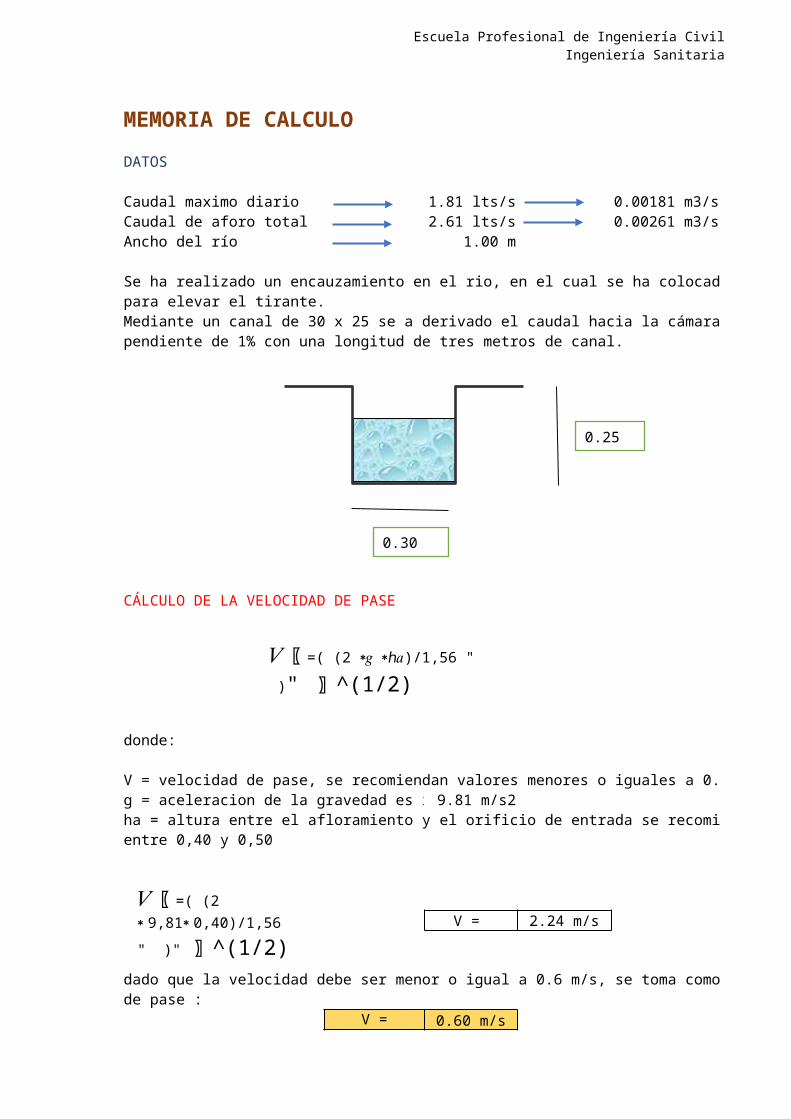
Se ha realizado un encauzamiento en el rio, en el cual se ha colocado una compuerta para elevar el tirante.Mediante un canal de 30 x 25 se a derivado el caudal hacia la cámara húmeda con una pendiente de 1% con una longitud de tres metros de canal.

CÁLCULO DE LA VELOCIDAD DE PASE

donde:

V = velocidad de pase, se recomiendan valores menores o iguales a 0.6 m/sg = aceleracion de la gravedad es igual 9.81 m/s2ha = altura entre el afloramiento y el orificio de entrada se recomiendan valoresentre 0,40 y 0,50

V = 2.24 m/s

dado que la velocidad debe ser menor o igual a 0.6 m/s, se toma como velocidadde pase :

V = 0.60 m/s

𝑉〖=( (2 )/1,56∗𝑔 ∗ℎ𝑎

" )" 〗̂ (1/2)

𝑉〖=( (2 ∗9,81∗0,40)/1,56

" )" 〗̂ (1/2)

0.25

0.30


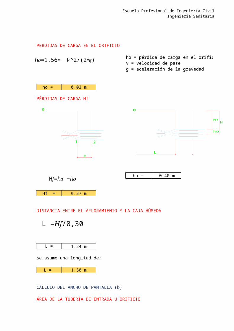
PERDIDAS DE CARGA EN EL ORIFICIO

ho = pérdida de carga en el orificiov = velocidad de paseg = aceleración de la gravedad

ho = 0.03 m

PÉRDIDAS DE CARGA Hf

ha = 0.40 m

Hf = 0.37 m

DISTANCIA ENTRE EL AFLORAMIENTO Y LA CAJA HÚMEDA

L = 1.24 m

se asume una longitud de:

L = 1.50 m

CÁLCULO DEL ANCHO DE PANTALLA (b)

ÁREA DE LA TUBERÍA DE ENTRADA U ORIFICIO

ℎ𝑜=1,56∗ 𝑉^2/(2∗𝑔)

H𝑓=ℎ𝑎 −ℎ𝑜

L =𝐻𝑓/0,30

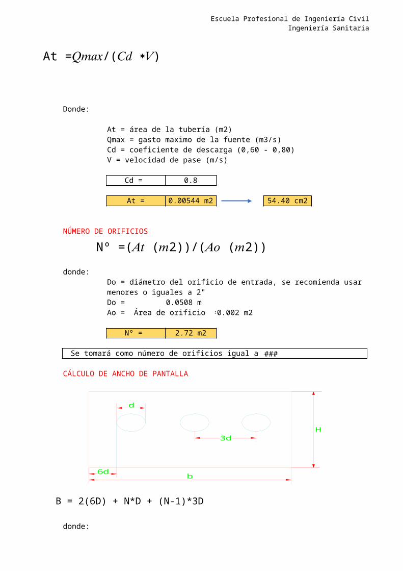
At =𝑄𝑚𝑎𝑥/(𝐶𝑑 ∗𝑉)

e

21

0H

Hf

ho

L

0


Donde:

At = área de la tubería (m2)Qmax = gasto maximo de la fuente (m3/s)Cd = coeficiente de descarga (0,60 - 0,80)V = velocidad de pase (m/s)

Cd = 0.8

At = 0.00544 m2 54.40 cm2

NÚMERO DE ORIFICIOS

donde: Do = diámetro del orificio de entrada, se recomienda usar diámetros menores o iguales a 2"Do = 0.0508 mAo = Área de orificio = 0.002 m2

Nº = 2.72 m2

Se tomará como número de orificios igual a 3 orificios

CÁLCULO DE ANCHO DE PANTALLA

donde:D = diámetro de orificios (m)

At =𝑄𝑚𝑎𝑥/(𝐶𝑑 ∗𝑉)

Nº =(𝐴𝑡 (𝑚2))/(𝐴𝑜 (𝑚2))

B = 2(6D) + N*D + (N-1)*3D

3d

d

b6d

H


N = número de orificios

B = 1.07 m

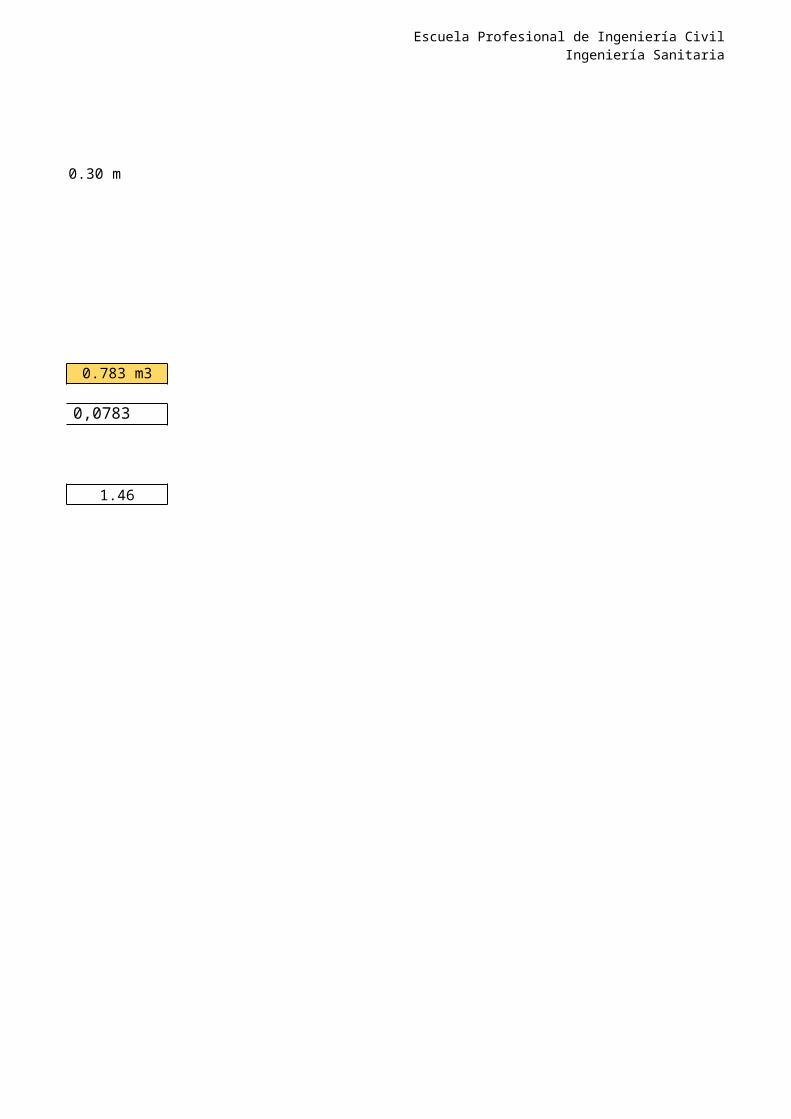
CÁLCULO DE VOLUMEN DE ALMACENAMIENTO

donde:tr = (3 - 5min)tr = 5min 300 seg

Va = 0.783 m3 783 lts

CÁLCULO DE DIÁMETRO DE SALIDA DE TUBERÍA DE CONDUCCIÓN

D salida = 1.96 ¨

El diámetro de salida a utilizar será de 2 ¨ 0.0508 m

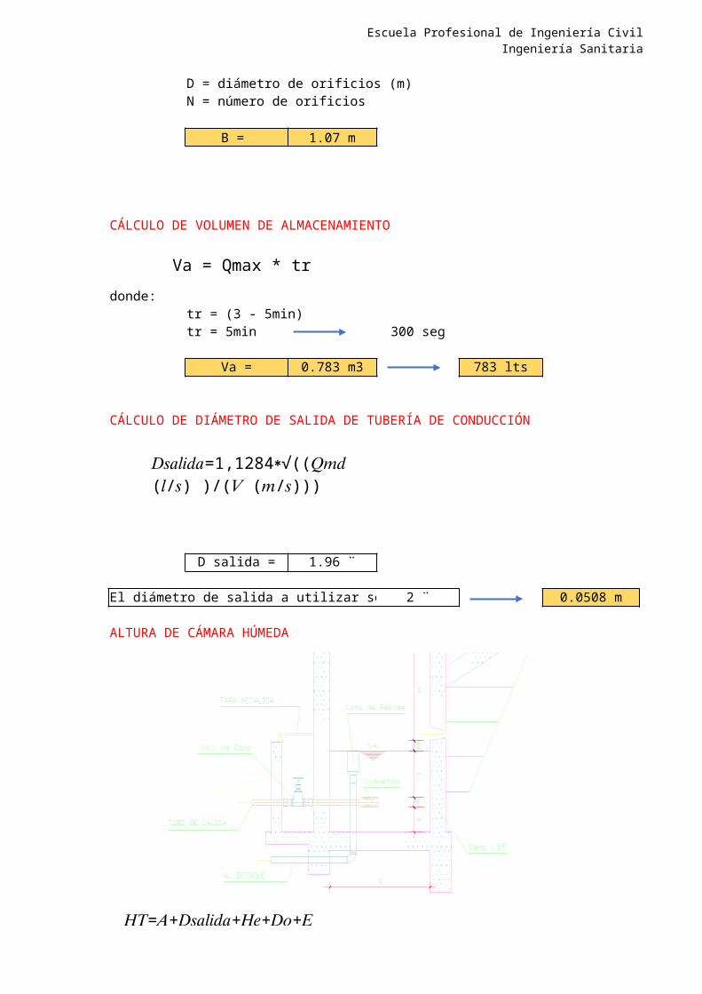
ALTURA DE CÁMARA HÚMEDA

Va = Qmax * tr

𝐷𝑠𝑎𝑙𝑖𝑑𝑎=1,1284∗√((𝑄𝑚𝑑 (𝑙/𝑠) )/(𝑉 (𝑚/𝑠)))

𝐻𝑇=𝐴+𝐷𝑠𝑎𝑙𝑖𝑑𝑎+𝐻𝑒+𝐷𝑜+𝐸


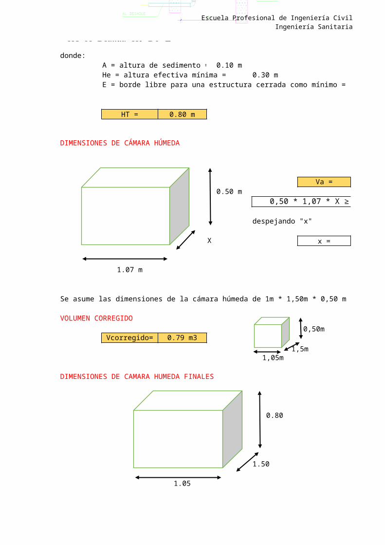
donde:A = altura de sedimento = 0.10 mHe = altura efectiva mínima = 0.30 mE = borde libre para una estructura cerrada como mínimo = 0.30 m

HT = 0.80 m

DIMENSIONES DE CÁMARA HÚMEDA

Va = 0.783 m30.50 m

despejando "x"

X x = 1.46

1.07 m

Se asume las dimensiones de la cámara húmeda de 1m * 1,50m * 0,50 m

VOLUMEN CORREGIDO

Vcorregido= 0.79 m3

DIMENSIONES DE CAMARA HUMEDA FINALES

0.80

1.50

1.05

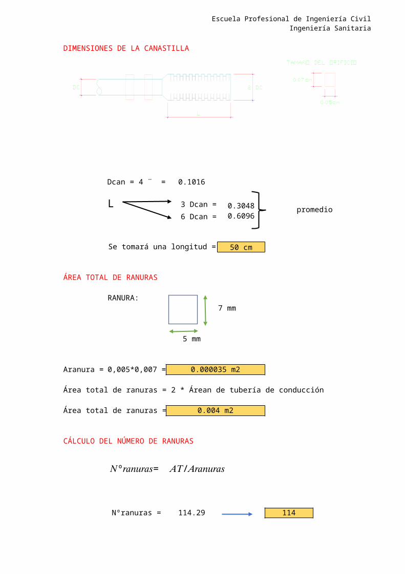
DIMENSIONES DE LA CANASTILLA

0,50 * 1,07 * X ≥ 0,0783

0,50m

1,5m1,05m


Dcan = 4 ¨ = 0.1016

L 3 Dcan = 0.3048 promedio 0.466 Dcan = 0.6096

Se tomará una longitud = 50 cm

ÁREA TOTAL DE RANURAS

RANURA:7 mm

5 mm

Aranura = 0,005*0,007 = 0.000035 m2

Área total de ranuras = 2 * Árean de tubería de conducción

Área total de ranuras = 0.004 m2

CÁLCULO DEL NÚMERO DE RANURAS

Nºranuras = 114.29 114

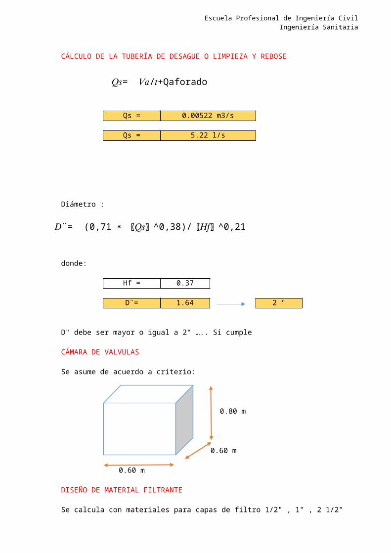
CÁLCULO DE LA TUBERÍA DE DESAGUE O LIMPIEZA Y REBOSE

𝑁º𝑟𝑎𝑛𝑢𝑟𝑎𝑠= 𝐴𝑇/𝐴𝑟𝑎𝑛𝑢𝑟𝑎𝑠


Qs = 0.00522 m3/s

Qs = 5.22 l/s

Diámetro :

donde:

Hf = 0.37

D¨= 1.64 2 "

D" debe ser mayor o igual a 2" ….. Si cumple

CÁMARA DE VALVULAS

Se asume de acuerdo a criterio:

0.80 m

0.60 m

0.60 m

DISEÑO DE MATERIAL FILTRANTE

Se calcula con materiales para capas de filtro 1/2" , 1" , 2 1/2"

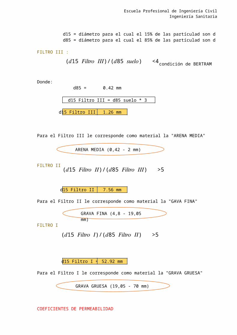
d15 = diámetro para el cual el 15% de las partículad son de menor tamaño

𝑄𝑠= 𝑉𝑎/𝑡+Qaforado

𝐷¨= (0,71 ∗ 〖𝑄𝑠〗 ^0,38)/ 〖𝐻𝑓〗 ^0,21


d85 = diámetro para el cual el 85% de las partículad son de menor tamaño

FILTRO III :

condición de BERTRAM

Donde:d85 = 0.42 mm

d15 Filtro III = d85 suelo * 3

d15 Filtro III = 1.26 mm

Para el Filtro III le corresponde como material la "ARENA MEDIA"

FILTRO II

d15 Filtro II = 7.56 mm

Para el Filtro II le corresponde como material la "GAVA FINA"

FILTRO I

d15 Filtro I = 52.92 mm

Para el Filtro I le corresponde como material la "GRAVA GRUESA"

COEFICIENTES DE PERMEABILIDAD

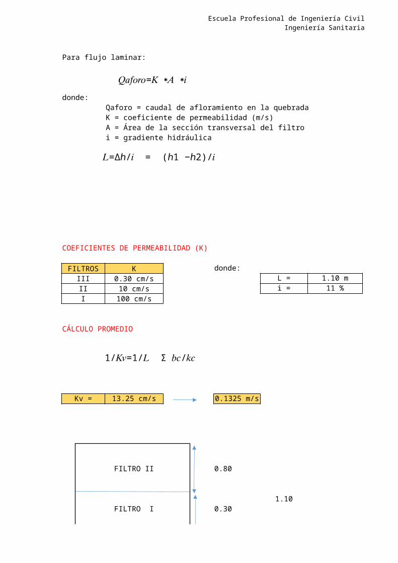
Para flujo laminar:

(𝑑15 𝐹𝑖𝑙𝑡𝑟𝑜 𝐼𝐼𝐼)/(𝑑85 𝑠𝑢𝑒𝑙𝑜) <4

ARENA MEDIA (0,42 - 2 mm)

(𝑑15 𝐹𝑖𝑙𝑡𝑟𝑜 𝐼𝐼)/(𝑑85 𝐹𝑖𝑙𝑡𝑟𝑜 𝐼𝐼𝐼) >5

GRAVA FINA (4,8 - 19,05 mm)

(𝑑15 𝐹𝑖𝑙𝑡𝑟𝑜 𝐼)/(𝑑85 𝐹𝑖𝑙𝑡𝑟𝑜 𝐼𝐼) >5

GRAVA GRUESA (19,05 - 70 mm)


donde:Qaforo = caudal de afloramiento en la quebradaK = coeficiente de permeabilidad (m/s)A = Área de la sección transversal del filtroi = gradiente hidráulica

COEFICIENTES DE PERMEABILIDAD (K)

FILTROS K donde:III 0.30 cm/s L = 1.10 mII 10 cm/s i = 11 %I 100 cm/s

CÁLCULO PROMEDIO

Kv = 13.25 cm/s 0.1325 m/s

FILTRO II 0.80

1.10FILTRO I 0.30

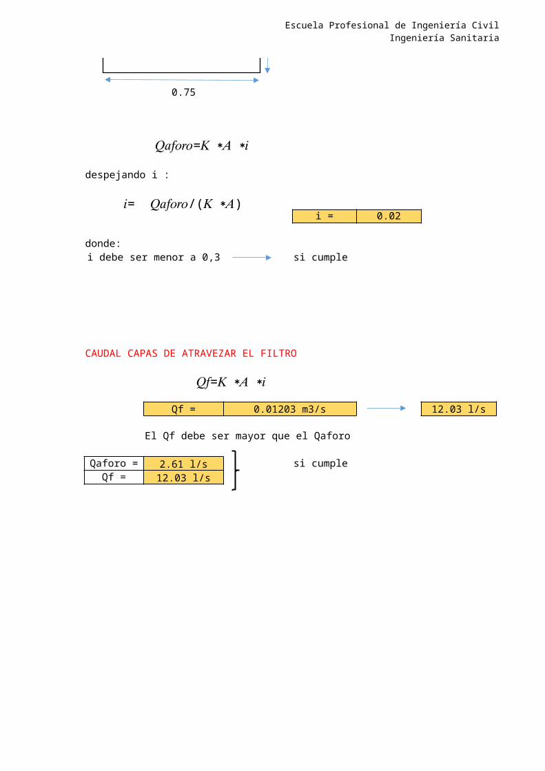
𝑄𝑎𝑓𝑜𝑟𝑜=𝐾 ∗𝐴 ∗𝑖

𝐿=∆ℎ/𝑖 = (ℎ1 −ℎ2)/𝑖

1/𝐾𝑣=1/𝐿 Σ 𝑏𝑐/𝑘𝑐


0.75

despejando i :

i = 0.02

donde:i debe ser menor a 0,3 si cumple

CAUDAL CAPAS DE ATRAVEZAR EL FILTRO

Qf = 0.01203 m3/s 12.03 l/s

El Qf debe ser mayor que el Qaforo

Qaforo = 2.61 l/s si cumpleQf = 12.03 l/s

𝑄𝑎𝑓𝑜𝑟𝑜=𝐾 ∗𝐴 ∗𝑖𝑖= 𝑄𝑎𝑓𝑜𝑟𝑜/(𝐾 ∗𝐴)

𝑄𝑓=𝐾 ∗𝐴 ∗𝑖

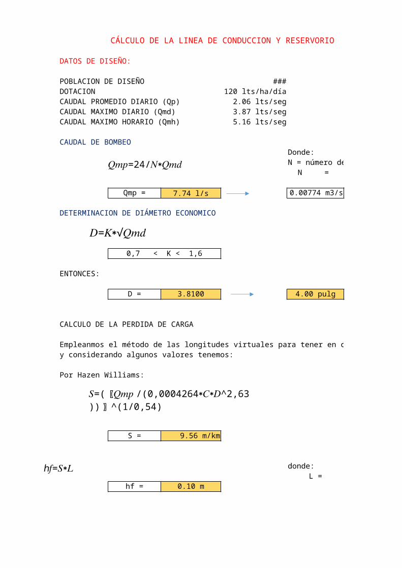
CÁLCULO DE LA LINEA DE CONDUCCION Y RESERVORIO

DATOS DE DISEÑO:

POBLACION DE DISEÑO 1360 habitantesDOTACION 120 lts/ha/díaCAUDAL PROMEDIO DIARIO (Qp) 2.06 lts/segCAUDAL MAXIMO DIARIO (Qmd) 3.87 lts/segCAUDAL MAXIMO HORARIO (Qmh) 5.16 lts/seg

CAUDAL DE BOMBEODonde:N = número de horas de bombeo

N = 12 horas

Qmp = 7.74 l/s 0.00774 m3/s

DETERMINACION DE DIÁMETRO ECONOMICO

ENTONCES:

D = 3.8100 4.00 pulg

CALCULO DE LA PERDIDA DE CARGA

Empleanmos el método de las longitudes virtuales para tener en cuenta las pérdidas localesy considerando algunos valores tenemos:

Por Hazen Williams:

S = 9.56 m/km

donde:L = 0.01000 km

hf = 0.10 m

0,7 < K < 1,6

𝑄𝑚𝑝=24/𝑁∗𝑄𝑚𝑑

𝐷=𝐾∗√𝑄𝑚𝑑

𝑆=( 〖𝑄𝑚𝑝 /(0,0004264∗𝐶∗𝐷^2,63 )) 〗 ^(1/0,54)

ℎ𝑓=𝑆∗𝐿

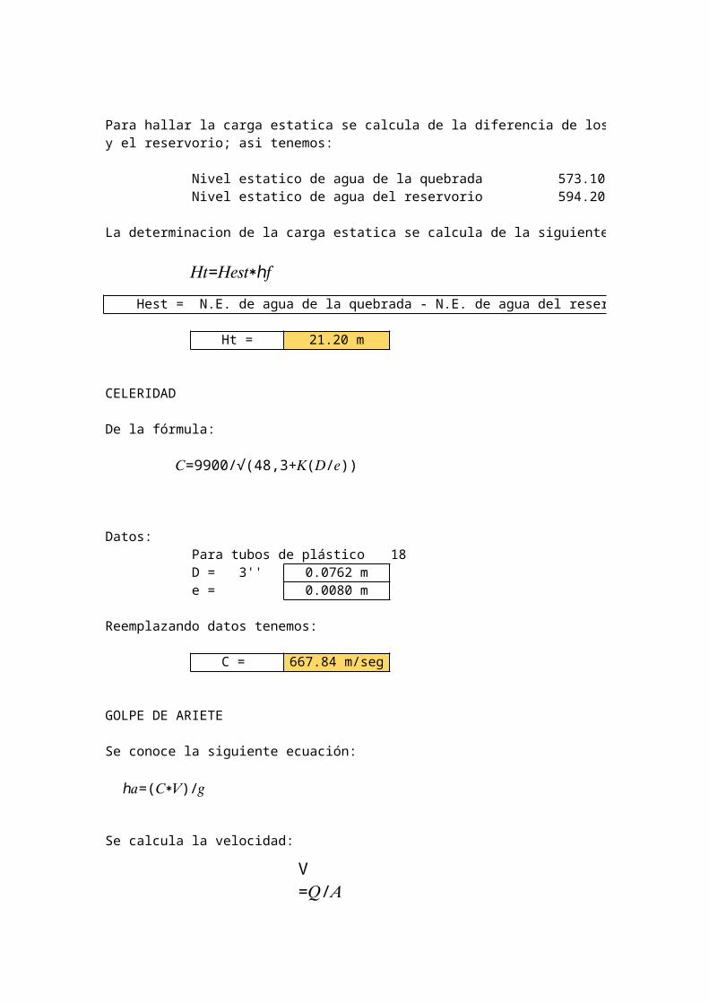
Para hallar la carga estatica se calcula de la diferencia de los desniveles de agua del pozoy el reservorio; asi tenemos:

Nivel estatico de agua de la quebrada 573.10Nivel estatico de agua del reservorio 594.20

La determinacion de la carga estatica se calcula de la siguiente manera:

Hest = N.E. de agua de la quebrada - N.E. de agua del reservorio

Ht = 21.20 m

CELERIDAD

De la fórmula:

Datos:Para tubos de plástico K= 18D = 3'' = 0.0762 me = 0.0080 m

Reemplazando datos tenemos:

C = 667.84 m/seg

GOLPE DE ARIETE

Se conoce la siguiente ecuación:

Se calcula la velocidad:

𝐻𝑡=𝐻𝑒𝑠𝑡∗ℎ𝑓

𝐶=9900/√(48,3+𝐾(𝐷/𝑒))

ℎ𝑎=(𝐶∗𝑉)/𝑔

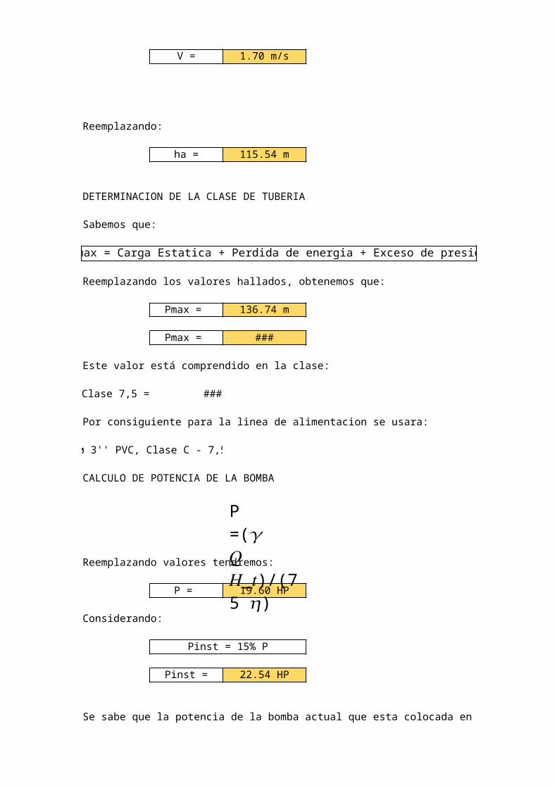
V =𝑄/𝐴

V = 1.70 m/s

Reemplazando:

ha = 115.54 m

DETERMINACION DE LA CLASE DE TUBERIA

Sabemos que:

Pmax = Carga Estatica + Perdida de energia + Exceso de presión

Reemplazando los valores hallados, obtenemos que:

Pmax = 136.74 m

Pmax = 136.74 lb/pulg2

Este valor está comprendido en la clase:

Clase 7,5 = 105 lb/pulg2

Por consiguiente para la linea de alimentacion se usara:

ø 3'' PVC, Clase C - 7,5

CALCULO DE POTENCIA DE LA BOMBA

Reemplazando valores tendremos:

P = 19.60 HP

Considerando:

Pinst = 15% P

Pinst = 22.54 HP

Se sabe que la potencia de la bomba actual que esta colocada en la caseta de

P =(𝛾 𝑄 𝐻_𝑡)/(75 𝜂)

Bombeo es de 10 HP, luego esta cubre lo proyectado.

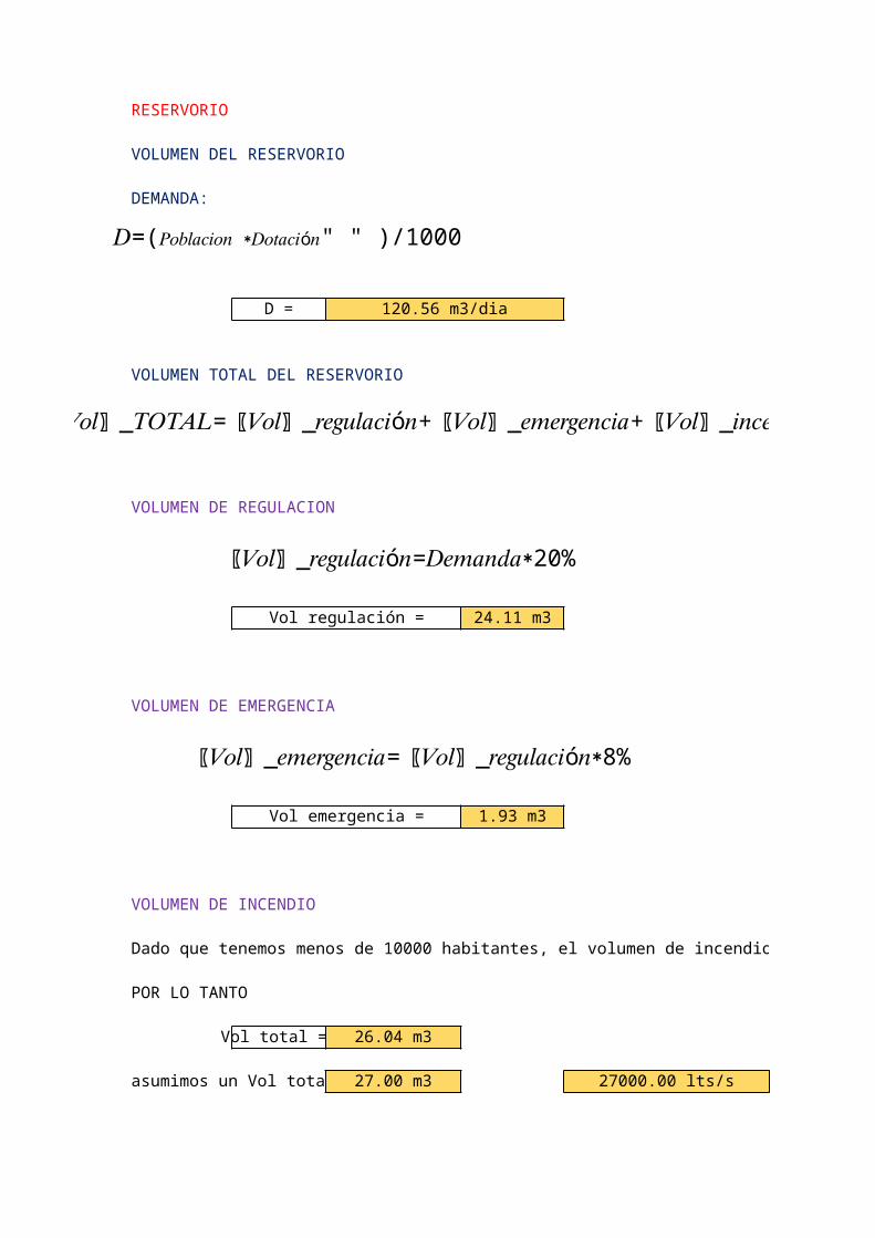
RESERVORIO

VOLUMEN DEL RESERVORIO

DEMANDA:

D = 120.56 m3/dia

VOLUMEN TOTAL DEL RESERVORIO

VOLUMEN DE REGULACION

Vol regulación = 24.11 m3

VOLUMEN DE EMERGENCIA

Vol emergencia = 1.93 m3

VOLUMEN DE INCENDIO

Dado que tenemos menos de 10000 habitantes, el volumen de incendio es igual a cero.

POR LO TANTO

Vol total = 26.04 m3

asumimos un Vol total de 27.00 m3 27000.00 lts/s

𝐷=(𝑃𝑜𝑏𝑙𝑎𝑐𝑖𝑜𝑛 ∗𝐷𝑜𝑡𝑎𝑐𝑖ó𝑛" " )/1000

〖〗𝑉𝑜𝑙 _𝑇𝑂𝑇𝐴𝐿=〖𝑉𝑜𝑙〗_𝑟𝑒𝑔𝑢𝑙𝑎𝑐𝑖ó𝑛+〖〗𝑉𝑜𝑙 _𝑒𝑚𝑒𝑟𝑔𝑒𝑛𝑐𝑖𝑎+〖〗𝑉𝑜𝑙 _𝑖𝑛𝑐𝑒𝑛𝑑𝑖𝑜

〖𝑉𝑜𝑙〗_𝑟𝑒𝑔𝑢𝑙𝑎𝑐𝑖ó𝑛=𝐷𝑒𝑚𝑎𝑛𝑑𝑎∗20%

〖𝑉𝑜𝑙〗_𝑒𝑚𝑒𝑟𝑔𝑒𝑛𝑐𝑖𝑎=〖〗𝑉𝑜𝑙 _𝑟𝑒𝑔𝑢𝑙𝑎𝑐𝑖ó𝑛∗8%

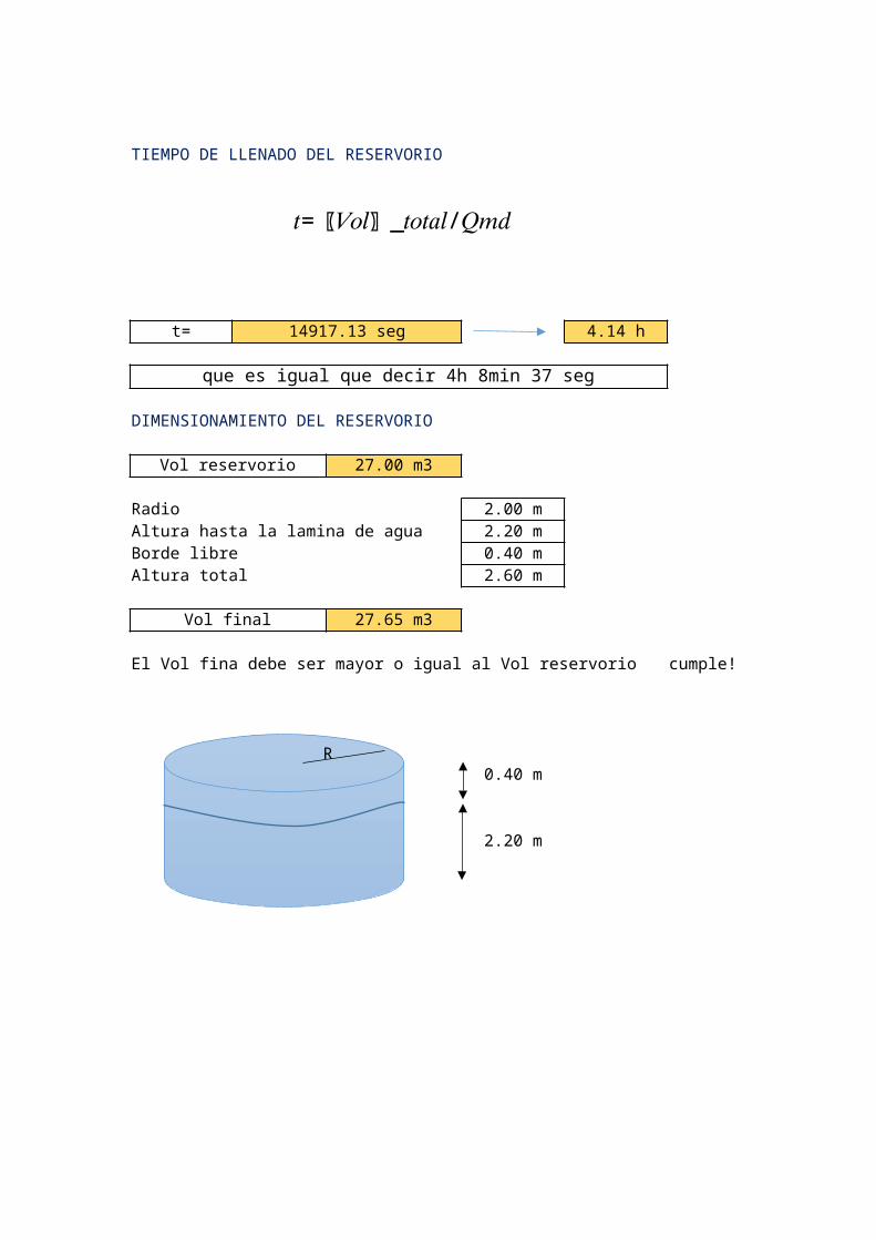
TIEMPO DE LLENADO DEL RESERVORIO

t= 14917.13 seg 4.14 h

que es igual que decir 4h 8min 37 seg

DIMENSIONAMIENTO DEL RESERVORIO

Vol reservorio 27.00 m3

Radio 2.00 mAltura hasta la lamina de agua 2.20 mBorde libre 0.40 mAltura total 2.60 m

Vol final 27.65 m3

El Vol fina debe ser mayor o igual al Vol reservorio cumple!

0.40 m

2.20 m

𝑡=〖〗𝑉𝑜𝑙 _𝑡𝑜𝑡𝑎𝑙/𝑄𝑚𝑑

R

〖〗𝑉𝑜𝑙 _𝑇𝑂𝑇𝐴𝐿=〖𝑉𝑜𝑙〗_𝑟𝑒𝑔𝑢𝑙𝑎𝑐𝑖ó𝑛+〖〗𝑉𝑜𝑙 _𝑒𝑚𝑒𝑟𝑔𝑒𝑛𝑐𝑖𝑎+〖〗𝑉𝑜𝑙 _𝑖𝑛𝑐𝑒𝑛𝑑𝑖𝑜

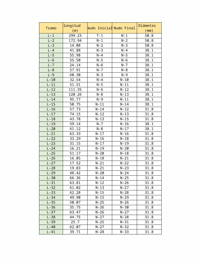
Tramo Nudo Inicial Nudo Final Material

L-1 299.23 T-1 N-1 50.8 PVCL-2 172.94 N-1 N-2 50.8 PVCL-3 14.08 N-2 N-3 50.8 PVCL-4 41.88 N-3 N-4 38.1 PVCL-5 55.98 N-4 N-5 38.1 PVCL-6 55.50 N-5 N-6 38.1 PVCL-7 24.14 N-6 N-7 38.1 PVCL-8 57.91 N-7 N-8 38.1 PVCL-9 60.30 N-3 N-9 38.1 PVC

L-10 32.54 N-4 N-10 38.1 PVCL-11 51.51 N-5 N-11 38.1 PVCL-12 111.35 N-6 N-12 38.1 PVCL-13 120.26 N-8 N-13 38.1 PVCL-14 95.77 N-9 N-11 38.1 PVCL-15 50.75 N-11 N-14 38.1 PVCL-16 57.73 N-14 N-12 31.8 PVCL-17 74.15 N-12 N-13 31.8 PVCL-18 43.78 N-13 N-15 31.8 PVCL-19 59.14 N-7 N-16 38.1 PVCL-20 61.12 N-8 N-17 38.1 PVCL-21 63.33 N-17 N-16 31.8 PVCL-22 33.29 N-16 N-18 31.8 PVCL-23 31.15 N-17 N-19 31.8 PVCL-24 16.21 N-19 N-20 31.8 PVCL-25 51.17 N-20 N-18 31.8 PVCL-26 16.05 N-18 N-21 31.8 PVCL-27 17.52 N-21 N-22 31.8 PVCL-28 19.83 N-21 N-23 31.8 PVCL-29 48.42 N-20 N-24 31.8 PVCL-30 66.36 N-14 N-25 31.8 PVCL-31 63.81 N-12 N-26 31.8 PVCL-32 61.02 N-13 N-27 31.8 PVCL-33 62.28 N-15 N-28 31.8 PVCL-34 49.90 N-15 N-29 31.8 PVCL-35 50.07 N-25 N-26 31.8 PVCL-36 35.75 N-26 N-30 31.8 PVCL-37 63.47 N-26 N-27 31.8 PVCL-38 44.75 N-27 N-28 31.8 PVCL-39 25.7 N-25 N-31 31.8 PVCL-40 62.07 N-27 N-32 31.8 PVCL-41 39.71 N-28 N-33 31.8 PVC

longitud (m)

Diámetro (mm)

Nudo Elevacion

150 1.23 T-1 592.00150 1.17 N-1 565.00 20.10150 1.13 N-2 566.00 14.30150 1.11 N-3 563.59 16.30150 1.01 N-4 553.22 25.20150 0.89 N-5 545.42 31.40150 0.63 N-6 543.61 31.90150 0.28 N-7 544.30 30.90150 0.87 N-8 544.10 30.90150 0.04 N-9 560.71 17.90150 0.04 N-10 554.38 24.10150 0.18 N-11 546.98 29.80150 0.09 N-12 541.91 33.40150 0.79 N-13 541.47 33.50150 0.75 N-14 554.63 21.30150 0.50 N-15 540.87 34.00150 0.34 N-16 545.00 30.10150 0.21 N-17 544.10 30.90150 0.27 N-18 541.76 33.20150 0.10 N-19 537.23 37.70150 0.09 N-20 539.54 35.40150 0.22 N-21 540.25 34.70150 0.16 N-22 535.69 39.30150 0.10 N-23 536.00 38.90150 0.02 N-24 531.00 43.90150 0.14 N-25 557.78 17.60150 0.05 N-26 544.03 31.20150 0.05 N-27 542.68 32.30150 0.05 N-28 542.42 32.50150 0.46 N-29 542.04 32.90150 0.23 N-30 551.34 23.90150 0.09 N-31 559.22 16.20150 0.01 N-32 542.00 33.00150 0.09 N-33 543.00 31.90150 0.27150 0.10150 0.29150 0.18150 0.09150 0.09150 0.09

Hazen- Williams Velocidad (m/s) Presion

(mca)

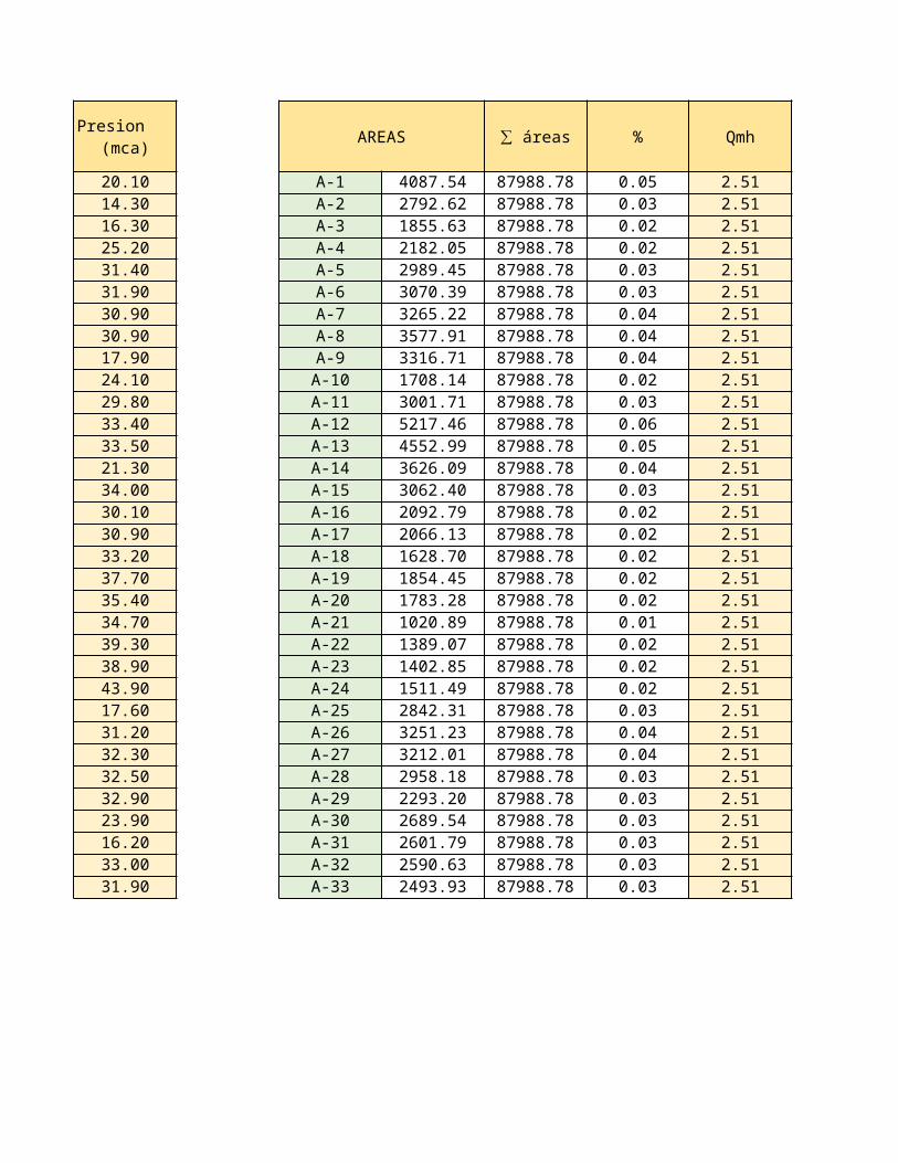
AREAS ∑ áreas % Qmh Qparcial

A-1 4087.54 87988.78 0.05 2.51 0.12A-2 2792.62 87988.78 0.03 2.51 0.08A-3 1855.63 87988.78 0.02 2.51 0.05A-4 2182.05 87988.78 0.02 2.51 0.06A-5 2989.45 87988.78 0.03 2.51 0.09A-6 3070.39 87988.78 0.03 2.51 0.09A-7 3265.22 87988.78 0.04 2.51 0.09A-8 3577.91 87988.78 0.04 2.51 0.10A-9 3316.71 87988.78 0.04 2.51 0.09

A-10 1708.14 87988.78 0.02 2.51 0.05A-11 3001.71 87988.78 0.03 2.51 0.09A-12 5217.46 87988.78 0.06 2.51 0.15A-13 4552.99 87988.78 0.05 2.51 0.13A-14 3626.09 87988.78 0.04 2.51 0.10A-15 3062.40 87988.78 0.03 2.51 0.09A-16 2092.79 87988.78 0.02 2.51 0.06A-17 2066.13 87988.78 0.02 2.51 0.06A-18 1628.70 87988.78 0.02 2.51 0.05A-19 1854.45 87988.78 0.02 2.51 0.05A-20 1783.28 87988.78 0.02 2.51 0.05A-21 1020.89 87988.78 0.01 2.51 0.03A-22 1389.07 87988.78 0.02 2.51 0.04A-23 1402.85 87988.78 0.02 2.51 0.04A-24 1511.49 87988.78 0.02 2.51 0.04A-25 2842.31 87988.78 0.03 2.51 0.08A-26 3251.23 87988.78 0.04 2.51 0.09A-27 3212.01 87988.78 0.04 2.51 0.09A-28 2958.18 87988.78 0.03 2.51 0.08A-29 2293.20 87988.78 0.03 2.51 0.07A-30 2689.54 87988.78 0.03 2.51 0.08A-31 2601.79 87988.78 0.03 2.51 0.07A-32 2590.63 87988.78 0.03 2.51 0.07A-33 2493.93 87988.78 0.03 2.51 0.07

2.51

Nº de viviendas 174

Poblacion final 998

Dotación 120

Qmh 2.51

DETERMINACION DE LOS CAUDALES DE DISEÑO

CAUDAL DE DESAGUE (Qd)

Qd = 2.01

CAUDAL DE LLUVIA (Qll)

Qll = 0.40

CAUDAL DE DISEÑO (Qd)

Qd = 2.41

qu = 0.014

TRAMO Nº VIVIENDAS Q inicial qu Qfinal Qtotal

B24-B23 3 0.000 0.014 0.042 0.042B22-B23 2 0.000 0.014 0.028 0.028B22-B21 2 0.000 0.014 0.028 0.028B21-B20 2 0.014 0.014 0.028 0.042B21-B31 7 0.014 0.014 0.097 0.111B20-B18 4 0.042 0.014 0.055 0.097B30-B31 3 0.000 0.014 0.042 0.042B31-B19 7 0.152 0.014 0.097 0.249B16-B17 2 0.000 0.014 0.028 0.028

𝑄𝑑=80%∗𝑄𝑚ℎ

𝑄𝑙𝑙=20%∗𝑄𝑑

𝑄𝑑=𝑄𝑙𝑙+𝑄𝑑

𝑞𝑢=𝑄𝑑/(𝑁º 𝑣𝑖𝑣𝑖𝑒𝑛𝑑𝑎𝑠)

B17-B18 0 0.014 0.014 0.000 0.014B18-B19 6 0.111 0.014 0.083 0.194B19-B15 11 0.443 0.014 0.152 0.595B16-B11 2 0.000 0.014 0.028 0.028B11-B12 8 0.014 0.014 0.111 0.125B11-B6 3 0.014 0.014 0.042 0.055B4-B3 1 0.000 0.014 0.014 0.014B3-B6 3 0.007 0.014 0.042 0.048B5-B6 4 0.000 0.014 0.055 0.055B6-B7 9 0.159 0.014 0.125 0.284B3-B2 4 0.007 0.014 0.055 0.062B1-B2 7 0.000 0.014 0.097 0.097B2-B7 3 0.159 0.014 0.042 0.201

B8-B13 7 0.000 0.014 0.097 0.097B13-B7 13 0.097 0.014 0.180 0.277B7-B12 1 0.762 0.014 0.014 0.776

B17-B12 4 0.014 0.014 0.055 0.069B12-B14 3 0.969 0.014 0.042 1.011B14-B15 2 1.011 0.014 0.028 1.039B15-B25 4 1.634 0.014 0.055 1.689B8-B25 2 0.000 0.014 0.028 0.028

B25-B26 5 1.717 0.014 0.069 1.786B8-B9 11 0.000 0.014 0.152 0.152

B26-B9 7 0.893 0.014 0.097 0.990B9-B10 3 1.142 0.014 0.042 1.184

B10-B28 1 1.184 0.014 0.014 1.198B26-B27 5 0.893 0.014 0.069 0.962B27-B28 8 0.481 0.014 0.111 0.592B28-B29 1 1.790 0.014 0.014 1.804B29-B33 0 1.804 0.014 0.000 1.804B27-B32 2 0.481 0.014 0.028 0.509B32-B33 2 0.509 0.014 0.028 0.537

174

Q min Qusar Sn Qr S 0/000 Qo Qr/Qo

1.5 1.50 0.0045 1.50 5.34 23.96 0.061.5 1.50 0.0045 1.50 67.90 85.42 0.021.5 1.50 0.0045 1.50 109.53 108.49 0.011.5 1.50 0.0045 1.50 52.47 75.09 0.021.5 1.50 0.0045 1.50 258.38 166.63 0.011.5 1.50 0.0045 1.50 130.52 118.43 0.011.5 1.50 0.0045 1.50 40.79 66.21 0.021.5 1.50 0.0045 1.50 143.83 124.32 0.011.5 1.50 0.0045 1.50 56.93 78.22 0.02

1.5 1.50 0.0045 1.50 137.10 121.38 0.011.5 1.50 0.0045 1.50 52.00 74.75 0.021.5 1.50 0.0045 1.50 40.21 65.74 0.021.5 1.50 0.0045 1.50 276.17 172.27 0.011.5 1.50 0.0045 1.50 45.55 69.96 0.021.5 1.50 0.0045 1.50 49.20 72.71 0.021.5 1.50 0.0045 1.50 14.59 39.60 0.041.5 1.50 0.0045 1.50 5.73 24.81 0.061.5 1.50 0.0045 1.50 26.21 53.07 0.031.5 1.50 0.0045 1.50 15.39 40.67 0.041.5 1.50 0.0045 1.50 21.03 47.54 0.031.5 1.50 0.0045 1.50 23.13 49.86 0.031.5 1.50 0.0045 1.50 5.23 23.71 0.061.5 1.50 0.0045 1.50 21.67 48.26 0.031.5 1.50 0.0045 1.50 32.50 59.10 0.031.5 1.50 0.0045 1.50 5.10 23.41 0.061.5 1.50 0.0045 1.50 241.00 160.93 0.011.5 1.50 0.0045 1.50 8.21 29.70 0.051.5 1.50 0.0045 1.50 7.30 28.01 0.051.5 1.69 0.0043 1.69 31.30 58.00 0.031.5 1.50 0.0045 1.50 8.79 30.73 0.051.5 1.79 0.0042 1.79 5.16 23.55 0.081.5 1.50 0.0045 1.50 6.03 25.46 0.061.5 1.50 0.0045 1.50 8.78 30.72 0.051.5 1.50 0.0045 1.50 195.18 144.83 0.011.5 1.50 0.0045 1.50 8.58 30.37 0.051.5 1.50 0.0045 1.50 65.20 83.71 0.021.5 1.50 0.0045 1.50 78.74 91.99 0.021.5 1.80 0.0042 1.80 116.31 111.80 0.021.5 1.80 0.0042 1.80 40.11 65.65 0.031.5 1.50 0.0045 1.50 104.46 105.95 0.011.5 1.50 0.0045 1.50 139.94 122.63 0.01

Y Vr Vo Vr/Vo

0.16 0.704 0.763 0.9230.08 0.704 2.720 0.2590.04 0.704 3.455 0.2040.08 0.704 2.391 0.2940.04 0.704 5.307 0.1330.04 0.704 3.772 0.1870.08 0.704 2.109 0.3340.04 0.704 3.959 0.1780.08 0.704 2.491 0.283

0.04 0.704 3.866 0.1820.08 0.704 2.381 0.2960.08 0.704 2.093 0.3360.04 0.704 5.486 0.1280.08 0.704 2.228 0.3160.08 0.704 2.316 0.3040.13 0.704 1.261 0.5580.16 0.704 0.790 0.8910.10 0.704 1.690 0.4160.13 0.704 1.295 0.5430.10 0.704 1.514 0.4650.10 0.704 1.588 0.4430.16 0.704 0.755 0.9320.10 0.704 1.537 0.4580.10 0.704 1.882 0.3740.16 0.704 0.746 0.9440.04 0.704 5.125 0.1370.15 0.704 0.946 0.7440.15 0.704 0.892 0.7890.10 0.684 1.847 0.3710.15 0.704 0.979 0.7190.18 0.676 0.750 0.9010.16 0.704 0.811 0.8680.15 0.704 0.978 0.7200.04 0.704 4.612 0.1530.15 0.704 0.967 0.7280.08 0.704 2.666 0.2640.08 0.704 2.930 0.2400.08 0.674 3.561 0.1890.10 0.674 2.091 0.3220.04 0.704 3.374 0.2090.04 0.704 3.905 0.180

TABLA OBTENIDA DEL GRAFICO DE LOS ELEMENTOSHIDRAULICOS PROPORCIONALES

Para valores < de fq = 0.01 considerar fv = 0.20

fq = QR / QP fd = d / D fv = VR / VP fq = QR / QP fd = d / D

0.01 0.04 0.20 0.51 0.510.02 0.08 0.30 0.52 0.510.03 0.10 0.31 0.53 0.520.04 0.13 0.41 0.54 0.530.05 0.15 0.45 0.55 0.530.06 0.16 0.48 0.56 0.540.07 0.18 0.53 0.57 0.540.08 0.18 0.55 0.58 0.550.09 0.20 0.56 0.59 0.560.10 0.22 0.59 0.60 0.560.11 0.23 0.60 0.61 0.570.12 0.24 0.63 0.62 0.580.13 0.25 0.64 0.63 0.580.14 0.26 0.66 0.64 0.580.15 0.27 0.68 0.65 0.590.16 0.28 0.69 0.66 0.600.17 0.29 0.71 0.67 0.600.18 0.30 0.72 0.68 0.600.19 0.30 0.73 0.69 0.610.20 0.31 0.75 0.70 0.620.21 0.32 0.76 0.71 0.620.22 0.33 0.77 0.72 0.620.23 0.34 0.78 0.73 0.630.24 0.35 0.80 0.74 0.640.25 0.35 0.80 0.75 0.640.26 0.36 0.81 0.76 0.650.27 0.36 0.82 0.77 0.660.28 0.37 0.83 0.78 0.660.29 0.38 0.84 0.79 0.670.30 0.38 0.85 0.80 0.680.31 0.39 0.86 0.81 0.680.32 0.40 0.87 0.82 0.690.33 0.40 0.88 0.83 0.690.34 0.41 0.89 0.84 0.700.35 0.42 0.90 0.85 0.710.36 0.43 0.91 0.86 0.710.37 0.43 0.92 0.87 0.720.38 0.44 0.93 0.88 0.730.39 0.44 0.94 0.89 0.730.40 0.45 0.95 0.90 0.74

0.41 0.46 0.95 0.91 0.750.42 0.46 0.95 0.92 0.750.43 0.47 0.96 0.93 0.760.44 0.47 0.97 0.94 0.760.45 0.48 0.98 0.95 0.770.46 0.48 0.98 0.96 0.780.47 0.49 0.98 0.97 0.790.48 0.49 0.99 0.98 0.800.49 0.49 1.00 0.99 0.800.50 0.50 1.00

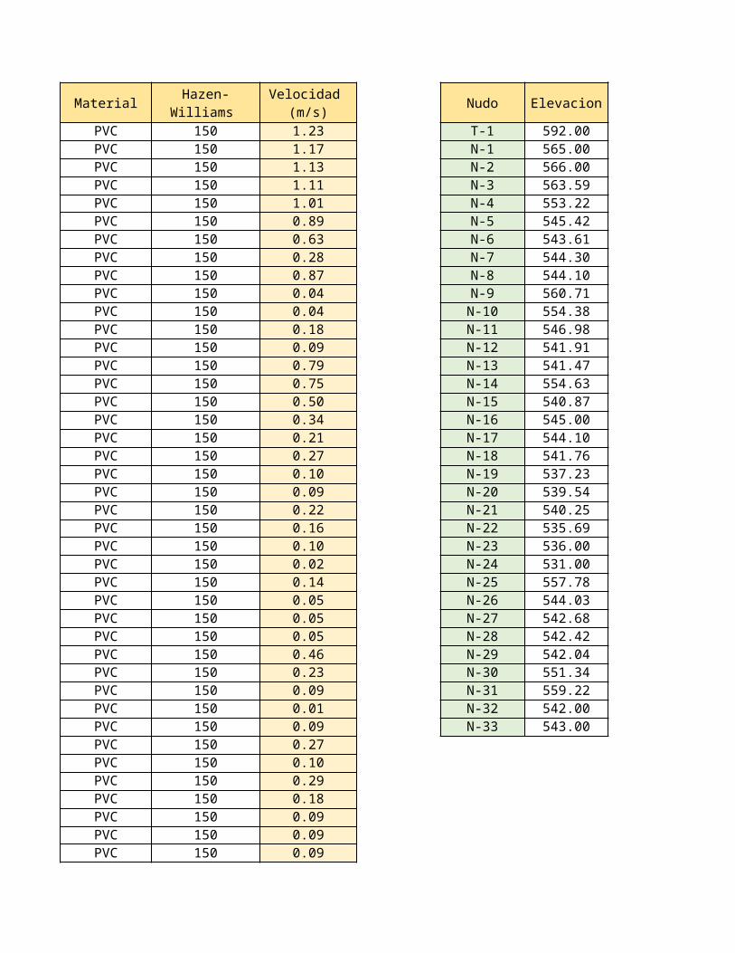
TABLA OBTENIDA DEL GRAFICO DE LOS ELEMENTOSHIDRAULICOS PROPORCIONALES

Para valores < de fq = 0.01 considerar fv = 0.20

fv = VR / VP

1.011.011.021.031.031.041.041.051.051.061.061.071.071.071.081.081.081.091.091.101.101.101.101.111.111.111.121.121.131.131.131.141.141.141.151.151.151.151.161.16

1.161.161.161.161.161.171.171.171.17

diseño-de-captacion (1)

Documents

Transcript of diseño-de-captacion (1)